a probabilistic seismic hazard analysis of northeast …home.iitk.ac.in/~vinaykg/pap64.pdfseismic...
TRANSCRIPT
A Probabilistic Seismic Hazard Analysis ofNortheast India
Sandip Das,a… Ishwer D. Gupta,b… and Vinay K. Guptaa…
Seismic hazard maps have been prepared for Northeast India based on theuniform hazard response spectra for absolute acceleration at stiff sites. Anapproach that is free from regionalizing the seismotectonic sources has beenproposed for performing the hazard analysis. Also, a new attenuation modelfor pseudo-spectral velocity scaling has been developed by using 261 recordedaccelerograms in Northeast India. In the present study, the entire area ofNortheast India has been divided into 0.1° grid size, and the hazard level hasbeen assessed for each node of this grid by considering the seismicity within a300-km radius around the node. Using the past earthquake data, the seismicityfor the area around each node has been evaluated by defining a and b values ofthe Gutenberg-Richter recurrence relationship, while accounting for theincompleteness of the earthquake catalogue. To consider the spatial dis-tribution of seismicity around each node, a spatially smoothed probabilitydistribution function of the observed epicentral distances has been used.Uniform hazard contours for pseudo-spectral acceleration as the hazardparameter have been obtained for an exposure time of 100 years and for 50%confidence level at different natural periods for both horizontal and verticalcomponents of ground motion. The trends reflected by these contours arebroadly consistent with the major seismotectonic features in the region.�DOI: 10.1193/1.2163914�
INTRODUCTION
Seismic hazard analysis plays an important role in the earthquake-resistant design ofstructures by providing a rational value of input hazard parameters, like peak groundacceleration �PGA� or the response spectrum amplitudes at different natural periods.Traditionally, PGA has been a popular hazard parameter, but it is often found to bepoorly correlated with the damage potential of ground motion. Hence it is increasinglybeing replaced by pseudo-spectral velocity �PSV� or pseudo-spectral acceleration �PSA�,which are considered to be more comprehensive in describing the hazard levels. All theexisting studies on seismic zoning of India have been made only in terms of the peakground acceleration and by using the attenuation relations for some other parts of theworld �Kaila and Rao 1979, Basu and Nigam 1978, Khattri et al. 1984, Bhatia et al.1999�. To utilize such studies for practical design applications, one needs to have a nor-malized spectral shape, which conceptually has several drawbacks �Trifunac 1992,Gupta 2002�. To overcome these shortcomings, a probabilistic seismic hazard analysis
a� Department of Civil Engineering, IIT Kanpur, Kanpur, UP 208016, Indiab�
Central Water and Power Research Station, Khadakwasla, Pune, Maharashtra 411024, India1Earthquake Spectra, Volume 22, No. 1, pages 1–27, February 2006; © 2006, Earthquake Engineering Research Institute
2 S. DAS, I. D. GUPTA, AND V. K. GUPTA
has been carried out in this study, and seismic hazard maps have been prepared forNortheast India1 in terms of the PSA amplitudes at different natural periods.
The advantages of the probabilistic seismic hazard analysis �PSHA� approach arewell known. The seismic hazard at a site is influenced by all the earthquakes with dif-ferent magnitudes and distances, and PSHA is able to correctly reflect the actual knowl-edge of seismicity �Orozova and Suhadolc 1999�. Along with the bigger events, smallerevents are also important in hazard estimation, due to their higher occurrence rates�Wheeler and Mueller 2001�. The essence of PSHA lies in the uniform hazard spectrum�UHS�, which is a convenient tool to compare the hazard representations of differentsites �Trifunac 1990, Todorovska et al. 1995, Peruzza et al. 2000�. PSHA can be carriedout in various ways depending on how one defines the model of seismicity.
To define the seismicity it is necessary to identify the various seismic sources in thearea of a site, and this generally requires considerable personal judgment. Use of mul-tiple scenarios is the latest development in the PSHA, wherein weights are assigned toeach possibility and the final results are obtained as the weighted average �Wahlströmand Grünthal 2001, Bernreuter et al. 1989, SSHAC 1997, EPRI 1986�. To avoid the per-sonal judgment and subjectivity, a regionalization-free approach has been proposed inthe present study based only on the available earthquake catalog data for about the past200 years without explicitly considering the hazard from known faults in the region.Other similar approaches have been proposed and used in the past by Veneziano et al.�1984�, Frankel �1995�, Woo �1996�, and many others. As the available data show goodcorrelation with all the known tectonic features in the Northeast India, the average trendof past seismicity can be considered to represent the future trend with good confidence.Therefore, earthquake recurrence relation is first defined by using all the past data withina 300-km radius of a site, with incompleteness of smaller magnitude earthquakes takeninto account. The total average seismicity represented by this recurrence relation is thendistributed with respect to distance by developing a smoothed probability distributionfunction of the epicentral distances of the past earthquakes from the site of interest. Inaddition to the seismicity, PSHA also requires an attenuation model specific to the re-gion that could be used to estimate the ground motion with a specified confidence levelfor any magnitude and distance combination. In the present case, a spectral attenuationrelationship is desirable since the target is to estimate the UHS at various sites of theregion. For Northeast India, no such attenuation relationship is available to date. Hencean attenuation model based on PSV scaling is developed by using a total of 261 accel-erograms from six different earthquake events.
To prepare the seismic hazard maps, the entire region of Northeast India is coveredby considering about 2,500 equally spaced sites. Seismicity for each of these sites is de-termined by defining the Gutenberg-Richter �G-R� magnitude-frequency relationship�Gutenberg and Richter 1944� using past earthquake events within a 300-km radius ofthe site. For obtaining the UHS at a site, the probability that a given value of PSV at a
1 Northeast India is the easternmost region of India, consisting of the following states: Nagaland, ArunachalPradesh, Mizoram, Manipur, Meghalaya, Tripura, and Assam. The states border Myanmar, Tibet, Bangladesh,
Nepal, and Bhutan, but only share a 50-km common border with the rest of India.
A PROBABILISTIC SEISMIC HAZARD ANALYSIS OF NORTHEAST INDIA 3
natural period will be exceeded is estimated by adopting the formulation of Andersonand Trifunac �1977� based on the Poissonian model of earthquake occurrences, thoughmore generalized models are also available �Lee 1992, Todorovska 1994�. With the haz-ard levels known at various sites in the form of several sets of UHS for different prob-abilities of exceedance, seismic hazard maps are obtained in terms of PSA contours for50% confidence level and an exposure period of 100 years. These maps are expected toprovide a more realistic distribution of seismic hazard at various wave periods than theuse of a map in terms of PGA and a standard spectral shape. However, these may not beappropriate for the purpose of building code, where large areas are generally character-ized by uniform hazard. Further, the proposed maps are only appropriate for relativelyshort return periods of ground motions and large probabilities of exceedance.
ATTENUATION MODEL FOR NORTHEAST INDIA
DATABASE USED
To develop a spectral attenuation model specific to Northeast India, a total of 261accelerograms recorded from six earthquake events at different stations in the regionhave been used. Table 1 lists the details of the contributing earthquakes, which span asurface wave magnitude range of 5.5 to 7.2 �the epicenters of these events are alsoshown in Figure 8 as filled circles�. These records are obtained from IIT Roorkee, anddetails of the data for the first four earthquakes are available in Chandrasekaran and Das�1993�. The focal depths of these earthquakes vary over a wide range of 15 km to122 km. In fact, Earthquakes #4, 5, and 6 are the subduction zone earthquakes, and onlyEarthquakes #1 and 3 are of crustal nature. Earthquake # 2 occurred in the interfacezone.
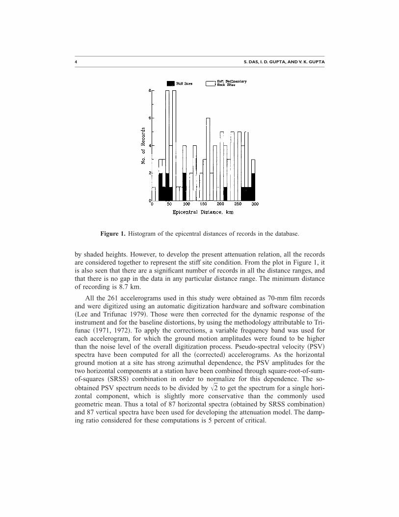
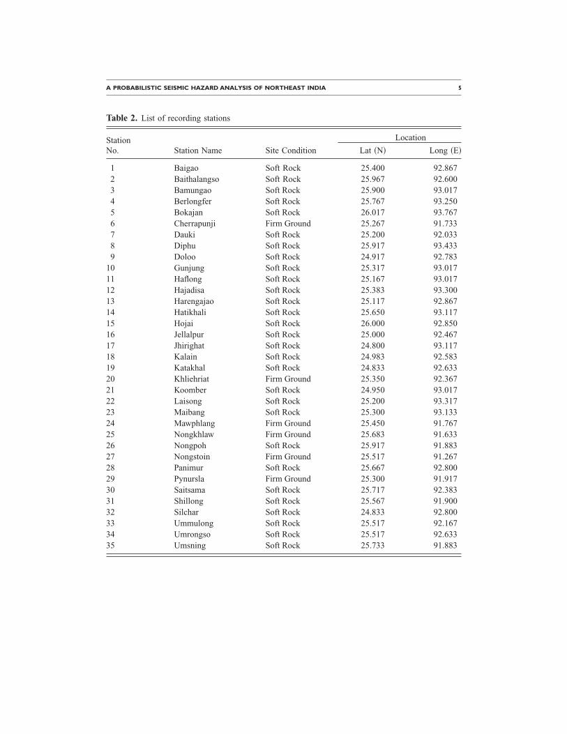
The number of three-component records contributed by each earthquake over epi-central distances up to 300 km is also indicated in Table 1. There are a total of 87 suchrecords providing a total of 261 acceleration components. The list of the recording sta-tions is given in Table 2. This indicates that all the records have been obtained either onstiff sites or on soft sedimentary rocks. Figure 1 shows the histogram of the epicentraldistances for all the records, with the number of the records on stiff soil sites indicated
Table 1. Details of the earthquakes contributing the strong motion data
Earthquake FocalEQ Name Epicenter Magnitude MMI Depth No. of# of EQ Date Lat �N� Long �E� MS Max. h �km� Records
1 Meghalaya 10 Sep 86 25.564 92.220 5.5 VI 28 112 N.E. India 18 May 87 25.479 93.598 5.7 V 50 143 N.E. India 6 Feb 88 25.500 91.460 5.8 VII 15 174 Burma Border 6 Aug 88 25.384 94.529 7.2 VII 91 285 W. Burma 10 Jan 90 24.750 95.240 6.1 VII 119 106 W. Burma 6 May 95 25.010 95.340 6.4 VI 122 7
4 S. DAS, I. D. GUPTA, AND V. K. GUPTA
by shaded heights. However, to develop the present attenuation relation, all the recordsare considered together to represent the stiff site condition. From the plot in Figure 1, itis also seen that there are a significant number of records in all the distance ranges, andthat there is no gap in the data in any particular distance range. The minimum distanceof recording is 8.7 km.
All the 261 accelerograms used in this study were obtained as 70-mm film recordsand were digitized using an automatic digitization hardware and software combination�Lee and Trifunac 1979�. Those were then corrected for the dynamic response of theinstrument and for the baseline distortions, by using the methodology attributable to Tri-funac �1971, 1972�. To apply the corrections, a variable frequency band was used foreach accelerogram, for which the ground motion amplitudes were found to be higherthan the noise level of the overall digitization process. Pseudo-spectral velocity �PSV�spectra have been computed for all the �corrected� accelerograms. As the horizontalground motion at a site has strong azimuthal dependence, the PSV amplitudes for thetwo horizontal components at a station have been combined through square-root-of-sum-of-squares �SRSS� combination in order to normalize for this dependence. The so-obtained PSV spectrum needs to be divided by �2 to get the spectrum for a single hori-zontal component, which is slightly more conservative than the commonly usedgeometric mean. Thus a total of 87 horizontal spectra �obtained by SRSS combination�and 87 vertical spectra have been used for developing the attenuation model. The damp-ing ratio considered for these computations is 5 percent of critical.
Figure 1. Histogram of the epicentral distances of records in the database.
A PROBABILISTIC SEISMIC HAZARD ANALYSIS OF NORTHEAST INDIA 5
Table 2. List of recording stations
LocationStationNo. Station Name Site Condition Lat �N� Long �E�
1 Baigao Soft Rock 25.400 92.8672 Baithalangso Soft Rock 25.967 92.6003 Bamungao Soft Rock 25.900 93.0174 Berlongfer Soft Rock 25.767 93.2505 Bokajan Soft Rock 26.017 93.7676 Cherrapunji Firm Ground 25.267 91.7337 Dauki Soft Rock 25.200 92.0338 Diphu Soft Rock 25.917 93.4339 Doloo Soft Rock 24.917 92.783
10 Gunjung Soft Rock 25.317 93.01711 Haflong Soft Rock 25.167 93.01712 Hajadisa Soft Rock 25.383 93.30013 Harengajao Soft Rock 25.117 92.86714 Hatikhali Soft Rock 25.650 93.11715 Hojai Soft Rock 26.000 92.85016 Jellalpur Soft Rock 25.000 92.46717 Jhirighat Soft Rock 24.800 93.11718 Kalain Soft Rock 24.983 92.58319 Katakhal Soft Rock 24.833 92.63320 Khliehriat Firm Ground 25.350 92.36721 Koomber Soft Rock 24.950 93.01722 Laisong Soft Rock 25.200 93.31723 Maibang Soft Rock 25.300 93.13324 Mawphlang Firm Ground 25.450 91.76725 Nongkhlaw Firm Ground 25.683 91.63326 Nongpoh Soft Rock 25.917 91.88327 Nongstoin Firm Ground 25.517 91.26728 Panimur Soft Rock 25.667 92.80029 Pynursla Firm Ground 25.300 91.91730 Saitsama Soft Rock 25.717 92.38331 Shillong Soft Rock 25.567 91.90032 Silchar Soft Rock 24.833 92.80033 Ummulong Soft Rock 25.517 92.16734 Umrongso Soft Rock 25.517 92.63335 Umsning Soft Rock 25.733 91.883

6 S. DAS, I. D. GUPTA, AND V. K. GUPTA
ATTENUATION RELATION
Prior to performing regression analysis on the PSV data, it is necessary to select afunctional form of attenuation model in terms of the parameters that govern the attenu-ation of ground shaking. In spite of apparent differences in the functional forms, an ex-amination of the various published attenuation relations �Douglas 2001, 2002� indicatesthat all of them include terms for geometrical spreading and magnitude scaling, withsome considering the anelastic attenuation effects also. Trifunac and coworkers �1980,1989� have proposed a functional form by using a frequency-dependent attenuationfunction in terms of a representative source-to-site distance �Trifunac and Lee 1990�,and by taking care of both horizontal and vertical motions simultaneously. The site soiland geological conditions in different published relations are defined and treated in awide variety of ways. As only a limited database is available and a detailed descriptionof the input parameters is lacking in the present situation, the following simplified formhas been used to describe the attenuation characteristics in the present study:
Figure 2. Variation of estimated �smoothed� regression coefficients with T.
A PROBABILISTIC SEISMIC HAZARD ANALYSIS OF NORTHEAST INDIA 7
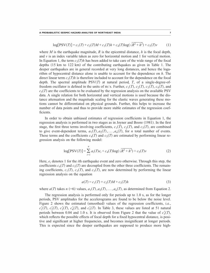
log�PSV�T�� = c1�T� + c2�T�M + c3�T�h + c4�T�log��R2 + h2� + c5�T�v �1�
where M is the earthquake magnitude, R is the epicentral distance, h is the focal depth,and v is an index variable taken as zero for horizontal motion and 1 for vertical motion.In Equation 1, the term c3�T�h has been added to take care of the wide range of the focaldepths �15 km to 122 km� of the contributing earthquakes as given in Table 1. Thedeeper earthquakes are in general recorded at very long distances, and hence the loga-rithm of hypocentral distance alone is unable to account for the dependence on h. Thedirect linear term c3�T�h is therefore included to account for the dependence on the focaldepth. The spectral amplitude PSV�T� at natural period, T, of a single-degree-of-freedom oscillator is defined in the units of m/s. Further, c1�T�, c2�T�, c3�T�, c4�T�, andc5�T� are the coefficients to be evaluated by the regression analysis on the available PSVdata. A single relation for both horizontal and vertical motions is used because the dis-tance attenuation and the magnitude scaling for the elastic waves generating these mo-tions cannot be differentiated on physical grounds. Further, this helps to increase thenumber of data points and thus to provide more stable estimates of the regression coef-ficients.
In order to obtain unbiased estimates of regression coefficients in Equation 1, theregression analysis is performed in two stages as in Joyner and Boore �1981�. In the firststage, the first three terms involving coefficients, c1�T�, c2�T�, and c3�T�, are combinedto give event-dependent terms, a1�T� ,a2�T� , . . . ,an�T�, for n total number of events.These terms and the coefficients c4�T� and c5�T� are estimated by performing linear re-gression analysis on the following model:
log�PSV�T�� = �i=1
n
ai�T�ei + c4�T�log��R2 + h2� + c5�T�v �2�
Here, ei denotes 1 for the ith earthquake event and zero otherwise. Through this step, thecoefficients c4�T� and c5�T� are decoupled from the other three coefficients. The remain-ing coefficients, c1�T�, c2�T�, and c3�T�, are now determined by performing the linearregression analysis on the equation
a�T� = c1�T� + c2�T�M + c3�T�h �3�
where a�T� takes n �=6� values, a1�T� ,a2�T� , . . . ,an�T�, as determined from Equation 2.
The regression analysis is performed only for periods up to 1.0 s, as for the longerperiods, PSV amplitudes for the accelerograms are found to be below the noise level.Figure 2 shows the estimated �smoothed� values of the regression coefficients, i.e.,c1��T�, c2��T�, c3��T�, c4��T�, and c5��T�. In Table 3, these values are listed at 51 naturalperiods between 0.04 and 1.0 s. It is observed from Figure 2 that the value of c3��T�,which reflects the possible effects of focal depth for a fixed hypocentral distance, is posi-tive and significant at higher frequencies, and becomes insignificant at longer periods.This is expected since the deeper earthquakes are supposed to produce more high-
8 S. DAS, I. D. GUPTA, AND V. K. GUPTA
Table 3. Estimated �smoothed� values of the regression coefficients
Period, T c1��T� c2��T� c3��T� c4��T� c5��T� µ�T� ��T�
0.040 −0.4405 0.2993 0.0035 −0.9007 −0.4252 0.0140 0.21790.042 −0.4114 0.2981 0.0035 −0.8974 −0.4231 0.0145 0.21920.044 −0.3815 0.2969 0.0035 −0.8945 −0.4211 0.0154 0.22050.046 −0.3507 0.2955 0.0035 −0.8921 −0.4192 0.0166 0.22200.048 −0.3192 0.2942 0.0035 −0.8904 −0.4175 0.0183 0.22370.050 −0.2872 0.2928 0.0036 −0.8892 −0.4160 0.0203 0.22540.055 −0.2075 0.2895 0.0036 −0.8876 −0.4131 0.0258 0.23000.060 −0.1297 0.2864 0.0036 −0.8865 −0.4108 0.0313 0.23440.065 −0.0552 0.2837 0.0037 −0.8858 −0.4091 0.0364 0.23840.070 0.0148 0.2813 0.0037 −0.8855 −0.4084 0.0409 0.24200.075 0.0794 0.2794 0.0038 −0.8855 −0.4085 0.0447 0.24490.080 0.1386 0.2779 0.0038 −0.8859 −0.4097 0.0477 0.24710.085 0.1924 0.2768 0.0038 −0.8870 −0.4119 0.0499 0.24870.090 0.2413 0.2761 0.0038 −0.8890 −0.4152 0.0514 0.24980.095 0.2854 0.2757 0.0039 −0.8922 −0.4195 0.0522 0.25050.100 0.3249 0.2757 0.0039 −0.8969 −0.4247 0.0526 0.25100.110 0.3962 0.2765 0.0040 −0.9084 −0.4364 0.0525 0.25150.120 0.4609 0.2780 0.0041 −0.9211 −0.4489 0.0521 0.25200.130 0.5171 0.2804 0.0042 −0.9346 −0.4618 0.0513 0.25250.140 0.5631 0.2837 0.0043 −0.9482 −0.4749 0.0502 0.25300.150 0.5973 0.2879 0.0044 −0.9610 −0.4879 0.0489 0.25350.160 0.6190 0.2928 0.0044 −0.9720 −0.5004 0.0474 0.25400.170 0.6281 0.2983 0.0045 −0.9803 −0.5119 0.0458 0.25440.180 0.6252 0.3039 0.0045 −0.9854 −0.5222 0.0442 0.25480.190 0.6114 0.3094 0.0045 −0.9865 −0.5309 0.0427 0.25520.200 0.5879 0.3144 0.0045 −0.9837 −0.5376 0.0412 0.25560.220 0.5282 0.3235 0.0045 −0.9718 −0.5480 0.0384 0.25650.240 0.4623 0.3317 0.0045 −0.9563 −0.5562 0.0358 0.25740.260 0.3917 0.3390 0.0045 −0.9378 −0.5619 0.0331 0.25840.280 0.3180 0.3454 0.0045 −0.9169 −0.5654 0.0305 0.25930.300 0.2420 0.3512 0.0044 −0.8947 −0.5667 0.0278 0.26000.320 0.1647 0.3566 0.0044 −0.8719 −0.5661 0.0251 0.26030.340 0.0869 0.3617 0.0044 −0.8493 −0.5639 0.0224 0.26030.360 0.0097 0.3667 0.0043 −0.8279 −0.5605 0.0197 0.25980.380 −0.0657 0.3719 0.0043 −0.8082 −0.5563 0.0172 0.25890.400 −0.1376 0.3772 0.0043 −0.7909 −0.5517 0.0148 0.25780.420 −0.2040 0.3826 0.0042 −0.7766 −0.5471 0.0128 0.25640.440 −0.2626 0.3880 0.0041 −0.7656 −0.5430 0.0112 0.25500.460 −0.3114 0.3935 0.0041 −0.7582 −0.5397 0.0102 0.25370.480 −0.3490 0.3988 0.0040 −0.7545 −0.5376 0.0098 0.25260.500 −0.3751 0.4042 0.0039 −0.7545 −0.5368 0.0101 0.25170.550 −0.4217 0.4174 0.0036 −0.7603 −0.5368 0.0119 0.25000.600 −0.4611 0.4307 0.0033 −0.7679 −0.5375 0.0142 0.2486
A PROBABILISTIC SEISMIC HAZARD ANALYSIS OF NORTHEAST INDIA 9
frequency body-wave motions than the shallower earthquakes of the same magnitudeand hypocentral distance, due to less anelastic attenuation and greater stress drop �Mc-Garr 1984�.
By using the estimated regression coefficients, the estimated value of log�PSV�T��becomes
log�PSV��T�� = c1��T� + c2��T�M + c3��T�h + c4��T�log��R2 + h2� + c5��T�v �4�
With PSV�T� representing the actual values of PSV spectra for an accelerogram, the re-siduals ��T� for all 174 PSV spectra are calculated as
��T� = log�PSV�T�� − log�PSV��T�� �5�
The observed probability distribution of the residuals, i.e., p*���T��, at each period T canbe obtained from the percentiles of the observations below different amplitudes of ��T�as computed from Equation 5. However, assuming that the residuals follow a normaldistribution with the mean, µ�T�, and standard deviation, ��T�, the theoretical probabil-ity distribution can be defined as
p���T�� =1
��T��2��
−�
��T�
e−12� x−µ�T�
��T� 2
dx �6�
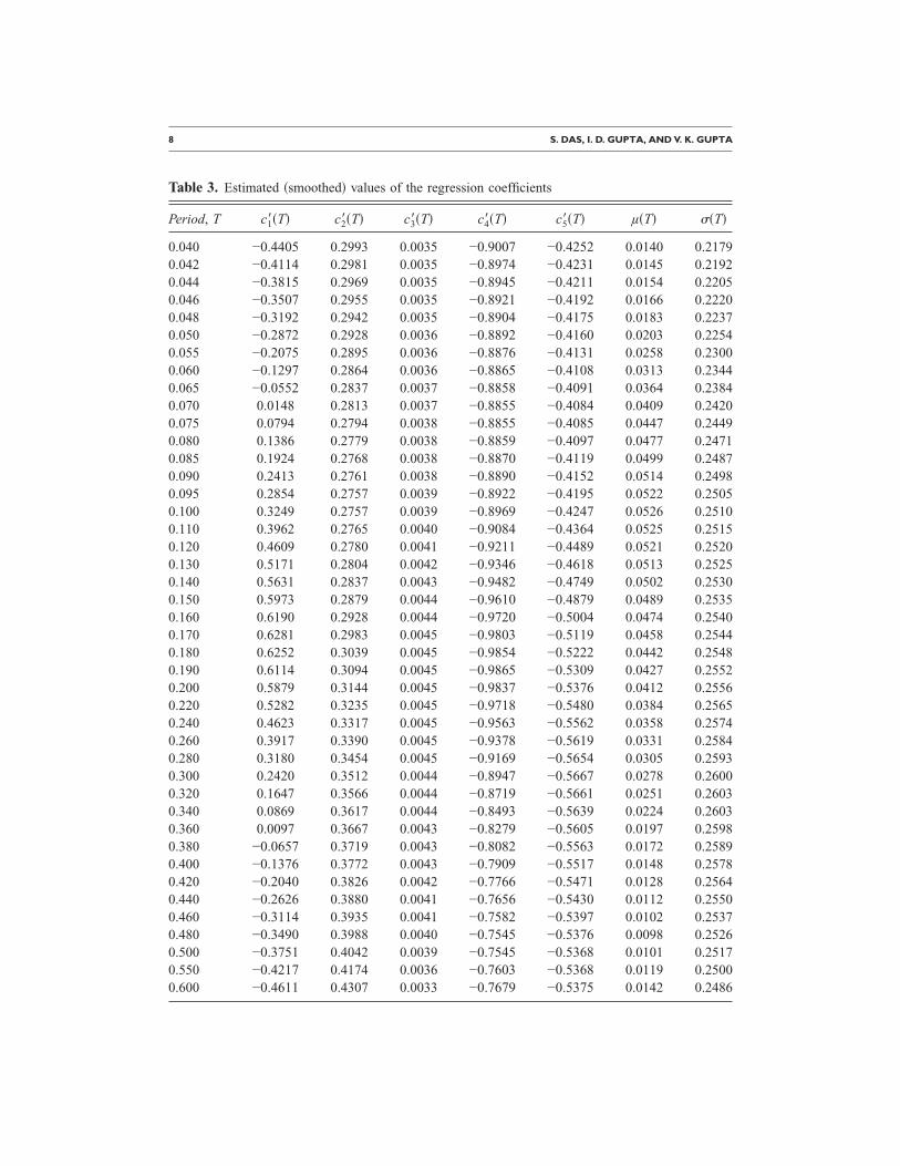
The maximum likelihood estimators of µ�T� and ��T� are calculated from p*���T���by calculating the mean and standard deviation of residuals at time period T�, and thenare smoothed along T. These smoothed values, say µ̂�T� and �̂�T�, are also shown inFigure 2 and listed in Table 3, which may be used to estimate ��T� at a given period T�by using Equation 6� corresponding to a specified level of confidence, p. Figure 3shows the comparison of these estimated residuals with the actual residuals, for p�� ,T�and p*�� ,T�=0.1 �10%� to 0.9 �90%�. The zig-zag solid lines in the figure represent theactual residuals, while the smooth dashed lines represent the estimated residuals. Thereliability of the assumption that residuals are normally distributed, has been checked bytwo well-known statistical “goodness-of-fit” tests, namely the chi-square andKolmogorov-Smirnov �KS� tests. Both tests have been conducted at 51 periods, and chi-
Table 3. �cont.�
Period, T c1��T� c2��T� c3��T� c4��T� c5��T� µ�T� ��T�
0.650 −0.4972 0.4438 0.0030 −0.7758 −0.5384 0.0166 0.24770.700 −0.5335 0.4566 0.0026 −0.7817 −0.5388 0.0187 0.24740.750 −0.5733 0.4684 0.0022 −0.7834 −0.5385 0.0204 0.24770.800 −0.6200 0.4789 0.0018 −0.7787 −0.5374 0.0213 0.24860.850 −0.6762 0.4881 0.0014 −0.7663 −0.5353 0.0213 0.25010.900 −0.7431 0.4960 0.0010 −0.7462 −0.5324 0.0205 0.25220.950 −0.8196 0.5030 0.0005 −0.7199 −0.5289 0.0189 0.25461.000 −0.9018 0.5096 0.0001 −0.6900 −0.5251 0.0170 0.2573
10 S. DAS, I. D. GUPTA, AND V. K. GUPTA
square statistics, �2�T�, and KS statistics, KS�T�, have been found to be well within their95% cut-off values at all the natural periods. Using the estimated residuals, ��p ,T�, andadding those to the least-square estimate as in Equation 4, the PSV spectrum for a de-sired level of confidence, p, may be obtained as
log�PSV��p,T�� = c1��T� + c2��T�M + c3��T�h + c4��T�log��R2 + h2� + c5��T�v + ��p,T��7�
ILLUSTRATION OF THE PROPOSED MODEL
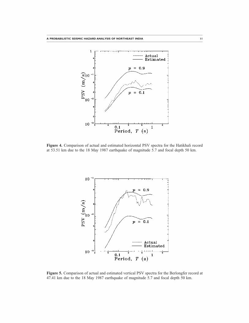
Figures 4 and 5 show typical comparison of the PSV spectra computed from the re-corded accelerograms, for a small and shallow event �18 May 1987� with M=5.7, h=50 km, with the PSV spectra estimated �by using Equation 7� for confidence levels of0.1 and 0.9. Figure 4 shows the comparison for the horizontal spectrum recorded at theHatikhali station with R=53.51 km, while Figure 5 shows the comparison for the verti-cal spectrum recorded at the Berlongfer station with R=47.41 km. In these figures, thepair of top �p=0.9� and bottom �p=0.1� PSV curves �in solid lines� outlines the 80%confidence interval of the predicted amplitudes, while the dashed line shows the actualspectrum. Figures 6 and 7 show similar comparison for a large and deep event �6 August1988� with M=7.2, h=91 km. Figure 6 shows the comparison for the horizontal spec-trum recorded at the Hajadisa station with R=123.50 km, while Figure 7 shows thecomparison for the vertical spectrum recorded at the Gunjung station with R=153.91 km.
It is clear from the above four figures that the proposed model works well for bothshallow and deep, and small and large events. It also works well for both near-source anddistant sites. However, the 80% confidence band is wide enough to reflect a considerable
Figure 3. Residual spectra for nine different values of p�� ,T� between 0.1 and 0.9 at intervalsof 0.1.
A PROBABILISTIC SEISMIC HAZARD ANALYSIS OF NORTHEAST INDIA 11
Figure 4. Comparison of actual and estimated horizontal PSV spectra for the Hatikhali record
at 53.51 km due to the 18 May 1987 earthquake of magnitude 5.7 and focal depth 50 km.Figure 5. Comparison of actual and estimated vertical PSV spectra for the Berlongfer record at
47.41 km due to the 18 May 1987 earthquake of magnitude 5.7 and focal depth 50 km.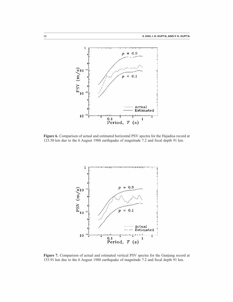
12 S. DAS, I. D. GUPTA, AND V. K. GUPTA
Figure 6. Comparison of actual and estimated horizontal PSV spectra for the Hajadisa record at
123.50 km due to the 6 August 1988 earthquake of magnitude 7.2 and focal depth 91 km.Figure 7. Comparison of actual and estimated vertical PSV spectra for the Gunjung record at
153.91 km due to the 6 August 1988 earthquake of magnitude 7.2 and focal depth 91 km.
A PROBABILISTIC SEISMIC HAZARD ANALYSIS OF NORTHEAST INDIA 13
amount of scatter, which is typical of strong motion data �Lee 2002�. This highlights thelevel of uncertainty that comes from the attenuation model alone in a probabilistic seis-mic hazard analysis.
PROBABILISTIC SEISMIC HAZARD FORMULATION
The probabilistic seismic hazard analysis is based on evaluating the probability dis-tribution function for the amplitudes, z, of a random parameter, Z, representing thestrong ground motion at a site due to all the earthquakes expected to occur during aspecified exposure period in the region around the site. Under the Poissonian assump-tion, this probability distribution is defined in terms of the annual rate, ��z�, of exceed-ing the ground motion level z at the site under consideration, due to all possible pairs,�M ,R�, of the magnitude and epicentral distance of the earthquake event expectedaround the site, with its random nature taken into account. To estimate the chance ofexceeding level z due to magnitude M at distance R, it is necessary to have an attenua-tion relation for the ground motion parameter Z, which in the present study has beentaken as the pseudo-spectral velocity, PSV�T�, at a given natural period, T.
Cornell �1968� was probably the first to present a formulation for probabilistic seis-mic hazard analysis. However, he proposed the use of only the median attenuation rela-tion to find ��z� as the sum total of the annual occurrence rates for all �M ,R� combina-tions, which produced the median ground motion level exceeding z. Thus the largerandom scattering of the recorded data that is normally present around the median at-tenuation was not accounted for in his formulation. Anderson and Trifunac �1978, 1977�incorporated the random uncertainties in the attenuation relations and defined the annualrate ��z� as
��z� = �i=1
I
�j=1
J
q�zMj,Ri�n�Mj,Ri� �8�
Here, q�z Mj ,Ri� is the probability of exceeding the ground motion level z due to anevent of size Mj at distance Ri. The quantity n�Mj ,Ri� is the annual rate of occurrence ofthe �Mj ,Ri� events. As the magnitude and distance are both continuous variables, forpractical applications, those are discretized into small intervals �Mj−�Mj /2 ,Mj
+�Mj /2� and �Ri−�Ri /2 ,Ri+�Ri /2� with central values, Mj and Ri. The summationsover i and j in Equation 8 are thus taken over the total number of distance intervals, I,and the magnitude intervals, J, respectively. Assuming that ��z� is the average occur-rence rate of a Poisson process, the probability of exceeding z during an exposure periodof Y years can be written as
P�Z � z� = 1 − exp�− Y��z�� �9�
The plot of z versus P�Z�z� is commonly termed as the hazard function.
The basic formulation constituted by the expressions of Equations 8 and 9 forms thecore of the state-of-the-art PSHA employing logic tree formulation to account for themodeling uncertainties. In the logic tree approach, one accounts for such uncertainties,

14 S. DAS, I. D. GUPTA, AND V. K. GUPTA
due to lack of data and incomplete understanding of the exact physical process, by con-sidering multiple scenarios with weights for the seismic source models, their expectedseismicity, and the ground motion attenuation relations. The basic PSHA as describedabove is then performed, for all possible sets of the input parameters, to obtain multipleestimates of ��z� with weights. These are used to get the expected �mean� value of ��z�,which is then used in Equation 9 to define the hazard function. In the present study, how-ever, a more objective regionalization-free approach has been proposed to define theseismicity rates n�Mj ,Ri�, as described in the next section. Also, only one model, as de-veloped in the previous section by using strong-motion data specific to Northeast India,has been used to estimate the probability q�z Mj ,Ri� for the PSV�T� amplitudes.
By using the PSHA formulation, the spectral amplitudes PSV�T� can be evaluated atall the natural periods for a constant probability of exceedance at a site. Such a responsespectrum is commonly known as the uniform hazard spectrum �UHS�. In addition toPSV, the functional can be any other property of ground motion, say, Fourier spectrumamplitude, power spectral density function, strong-motion duration, etc. In the presentstudy, the functional is considered to be PSA due to this being a popular design param-eter. For this, UHS is first obtained for the PSV functional �using the attenuation rela-tionship developed for PSV�, and then this is converted to the UHS for the PSA func-tional by multiplying with 2� /T.
SEISMICITY OF NORTHEAST INDIA
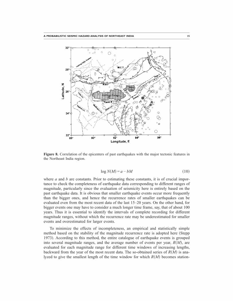
For seismic hazard analysis, the entire region of Northeast India lying between21°–30° latitude and 88°–97° longitude is considered. This is subdivided into a 0.1° lati-tude and 0.1° longitude grid, and the UHS are estimated for all the sites defined by theintersection points of the grid. For this purpose, the seismicity, n�Mj ,Ri�, for each site isevaluated by fitting the G-R recurrence relation to the past earthquake data within a300-km radius of the site, without identifying the seismotectonic source zones. Theearthquake catalogue used covers the period from 1458 to 2000, where the data up to1979 is taken from Bapat et al. �1983�, and from the USGS web site for the subsequentperiod. The data corresponds to the geographical area between 18°–33° latitude and85°–100° longitude. Figure 8 shows the correlation of the significant earthquakes, withmagnitude above 5.0, with the major tectonic features in Northeast India �Verma et al.1976�. It is seen that although the epicenters are dispersed widely, they definitely followthe trends of the tectonic features. Thus the identification of the seismic source zones isexpected to vary only slightly around the most likely trend defined by the epicentral dis-tribution. Also, the available database is quite comprehensive with a total of about 3,000events in the region of Figure 8. This can be used to estimate the expected occurrencerate of earthquakes in each magnitude range Mj, and to define in an objective way theirspatial distribution with respect to each site, as discussed in the following.
According to the G-R relationship, the annual occurrence rate, N�M�, of earthquakeswith magnitudes greater than or equal to M can be described by �Gutenberg and Richter1944�:
A PROBABILISTIC SEISMIC HAZARD ANALYSIS OF NORTHEAST INDIA 15
log N�M� = a − bM �10�
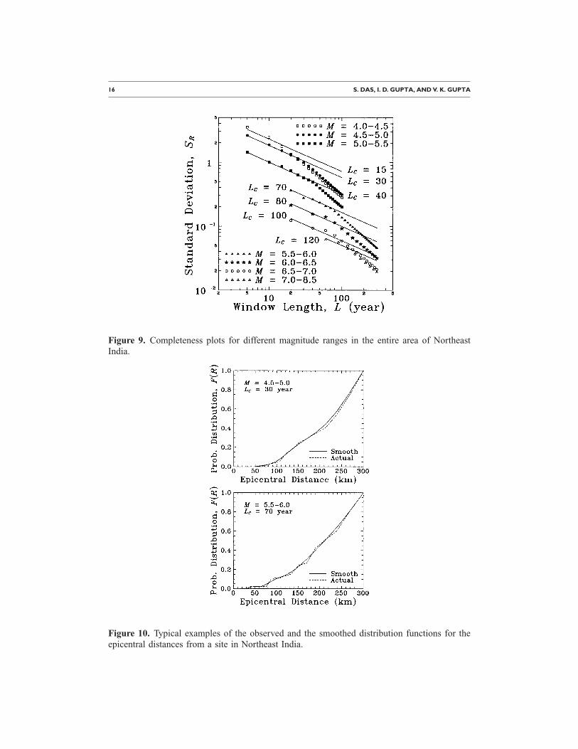
where a and b are constants. Prior to estimating these constants, it is of crucial impor-tance to check the completeness of earthquake data corresponding to different ranges ofmagnitude, particularly since the evaluation of seismicity here is entirely based on thepast earthquake data. It is obvious that smaller earthquake events occur more frequentlythan the bigger ones, and hence the recurrence rates of smaller earthquakes can beevaluated even from the most recent data of the last 15–20 years. On the other hand, forbigger events one may have to consider a much longer time frame, say, that of about 100years. Thus it is essential to identify the intervals of complete recording for differentmagnitude ranges, without which the recurrence rate may be underestimated for smallerevents and overestimated for larger events.
To minimize the effects of incompleteness, an empirical and statistically simplemethod based on the stability of the magnitude recurrence rate is adopted here �Stepp1973�. According to this method, the entire catalogue of earthquake events is groupedinto several magnitude ranges, and the average number of events per year, R�M�, areevaluated for each magnitude range for different time windows of increasing lengths,backward from the year of the most recent data. The so-obtained series of R�M� is ana-lyzed to give the smallest length of the time window for which R�M� becomes station-
Figure 8. Correlation of the epicenters of past earthquakes with the major tectonic features inthe Northeast India region.
16 S. DAS, I. D. GUPTA, AND V. K. GUPTA
Figure 9. Completeness plots for different magnitude ranges in the entire area of NortheastIndia.
Figure 10. Typical examples of the observed and the smoothed distribution functions for the
epicentral distances from a site in Northeast India.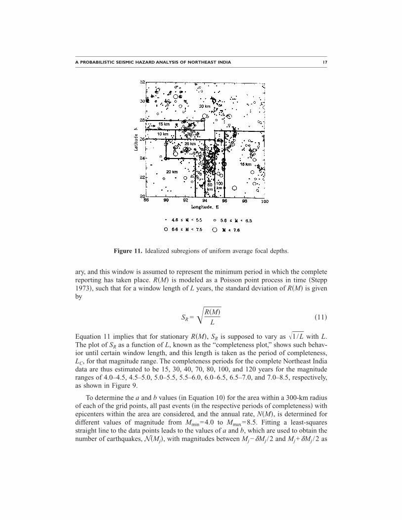
A PROBABILISTIC SEISMIC HAZARD ANALYSIS OF NORTHEAST INDIA 17
ary, and this window is assumed to represent the minimum period in which the completereporting has taken place. R�M� is modeled as a Poisson point process in time �Stepp1973�, such that for a window length of L years, the standard deviation of R�M� is givenby
SR =�R�M�L
�11�
Equation 11 implies that for stationary R�M�, SR is supposed to vary as �1/L with L.The plot of SR as a function of L, known as the “completeness plot,” shows such behav-ior until certain window length, and this length is taken as the period of completeness,LC, for that magnitude range. The completeness periods for the complete Northeast Indiadata are thus estimated to be 15, 30, 40, 70, 80, 100, and 120 years for the magnituderanges of 4.0–4.5, 4.5–5.0, 5.0–5.5, 5.5–6.0, 6.0–6.5, 6.5–7.0, and 7.0–8.5, respectively,as shown in Figure 9.
To determine the a and b values �in Equation 10� for the area within a 300-km radiusof each of the grid points, all past events �in the respective periods of completeness� withepicenters within the area are considered, and the annual rate, N�M�, is determined fordifferent values of magnitude from Mmin=4.0 to Mmax=8.5. Fitting a least-squaresstraight line to the data points leads to the values of a and b, which are used to obtain thenumber of earthquakes, N�Mj�, with magnitudes between Mj−�Mj /2 and Mj+�Mj /2 as
Figure 11. Idealized subregions of uniform average focal depths.
18 S. DAS, I. D. GUPTA, AND V. K. GUPTA
N�Mj� = N�Mj −�Mj
2 − N�Mj +
�Mj
2 �12�
It may be mentioned here that a maximum likelihood procedure �e.g., see Weichert1980� would have been better �in place of the least-squares method� to estimate the val-ues of a and b. However, since the Gutenberg-Richter’s relation has been defined for thecumulative number of earthquakes �which provides a normalizing effect for the residualoutliers�, care has been taken for the incompleteness in the smaller magnitudes, andsince a very small discretization interval of 0.1 has been used for the magnitude, thelimitations of the least-squares method may not be of much consequence to the accuracyof the estimates obtained here. Weichert �1980� has also indicated that for well-constrained data, the least-squares method may lead to the results equivalent to themaximum likelihood estimates.
To complete the description of seismicity, it is necessary to spatially distribute thenumbers N�Mj�, as obtained from Equation 12, with respect to the site. For this purpose,
Figure 12. Typical hazard curves for PSV amplitudes at different natural periods.
Figure 13. Uniform hazard PSA spectra �horizontal� for four different sites in Northeast India.
A PROBABILISTIC SEISMIC HAZARD ANALYSIS OF NORTHEAST INDIA 19
the epicentral distances from the site for all the events in a selected magnitude range,which occurred during the estimated period of completeness, are first used to define theobserved probability distribution function of the epicentral distance. To take care of the
Figure 14. Uniform hazard PSA spectra �vertical� for four different sites in Northeast India.
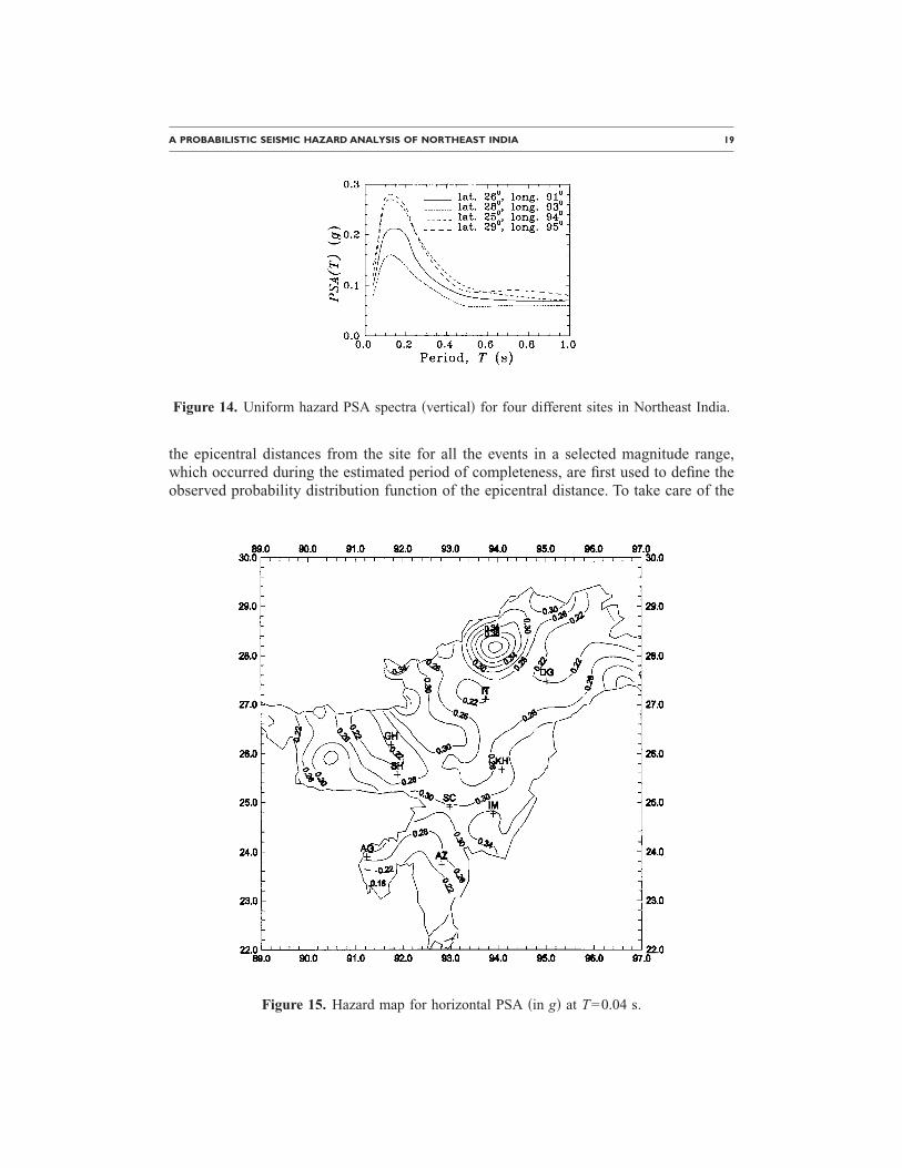
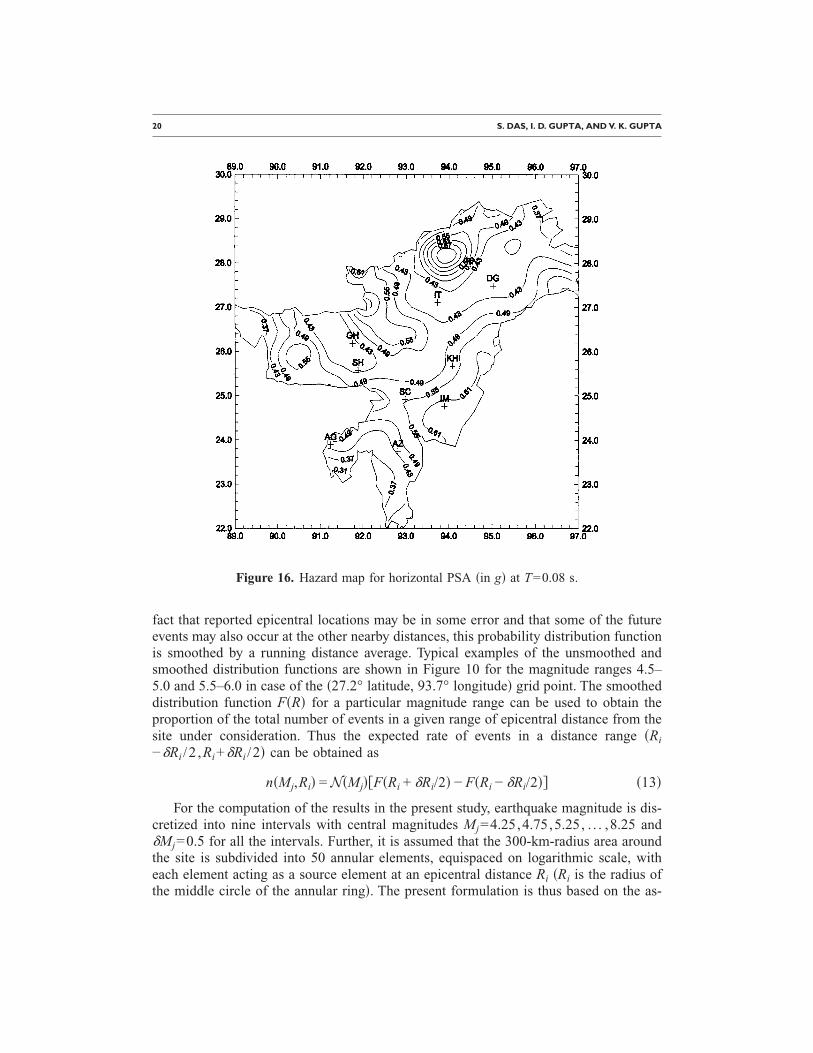
Figure 15. Hazard map for horizontal PSA �in g� at T=0.04 s.
20 S. DAS, I. D. GUPTA, AND V. K. GUPTA
fact that reported epicentral locations may be in some error and that some of the futureevents may also occur at the other nearby distances, this probability distribution functionis smoothed by a running distance average. Typical examples of the unsmoothed andsmoothed distribution functions are shown in Figure 10 for the magnitude ranges 4.5–5.0 and 5.5–6.0 in case of the �27.2° latitude, 93.7° longitude� grid point. The smootheddistribution function F�R� for a particular magnitude range can be used to obtain theproportion of the total number of events in a given range of epicentral distance from thesite under consideration. Thus the expected rate of events in a distance range �Ri
−�Ri /2 ,Ri+�Ri /2� can be obtained as
n�Mj,Ri� = N�Mj��F�Ri + �Ri/2� − F�Ri − �Ri/2�� �13�
For the computation of the results in the present study, earthquake magnitude is dis-cretized into nine intervals with central magnitudes Mj=4.25,4.75,5.25, . . . ,8.25 and�Mj=0.5 for all the intervals. Further, it is assumed that the 300-km-radius area aroundthe site is subdivided into 50 annular elements, equispaced on logarithmic scale, witheach element acting as a source element at an epicentral distance Ri �Ri is the radius ofthe middle circle of the annular ring�. The present formulation is thus based on the as-
Figure 16. Hazard map for horizontal PSA �in g� at T=0.08 s.

A PROBABILISTIC SEISMIC HAZARD ANALYSIS OF NORTHEAST INDIA 21
sumption of a point source. As explained in the next section, each combination of Mj
and Ri is also assigned a suitable focal depth to compute the probability of exceedancefor different values of spectral amplitudes. A consistent application of the parameters inthe attenuation relation developed and used in the present study is thus expected to pro-vide quite realistic estimate of UHS. However, if the earthquake source is considered tohave a finite rupture length and the distance Ri for each Mj is taken to be the closestdistance from the fault rupture, the results may be too conservative �Anderson and Tri-funac 1977, 1978�.
UNIFORM HAZARD MAPS FOR NORTHEAST INDIA
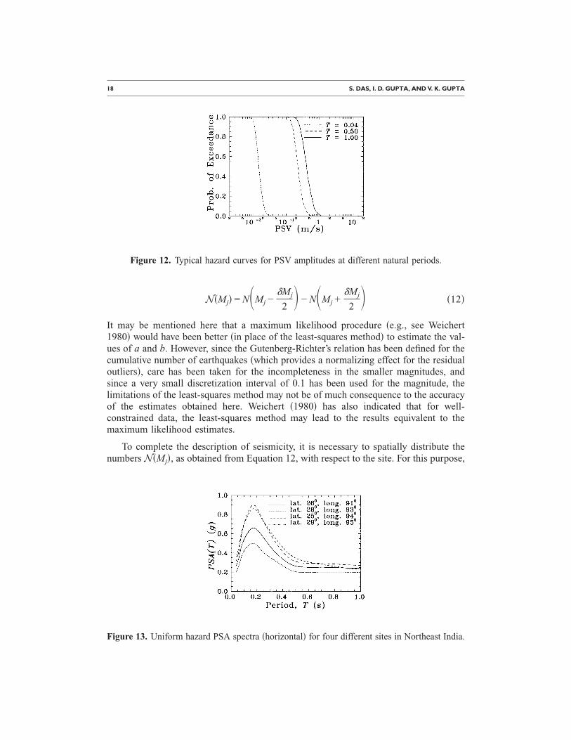
From the knowledge of n�Mj ,Ri� for a site in Northeast India, and for a given expo-sure period, the probability distribution of Equation 9 can be computed for the PSVspectrum at any specified natural period, T, by evaluating the probability,q�PSV�T� Mj ,Ri�, from the attenuation relation developed �see Equation 7�. For thecomputation of q�PSV�T� Mj ,Ri�, it is also necessary to assign the focal depth to eachcombination of Mj and Ri for the seismicity around the site. For this purpose, the depthsections of past earthquakes have been analyzed along several profiles transverse to the
Figure 17. Hazard map for horizontal PSA �in g� at T=0.17 s.
22 S. DAS, I. D. GUPTA, AND V. K. GUPTA
major tectonic features in the region, and uniform average focal depths are assigned tothe earthquakes in different areas of Northeast India as shown in Figure 11. The num-bers, n�Mj ,Ri�, are then subdivided into numbers for different average focal depths onthe basis of the observed number of events for each value of the average focal depth.
Figure 12 shows the probability distribution of Equation 9, as computed for T=0.04, 0.50, and 1.0 s, in the case of the horizontal component for the �27.2° latitude,93.7° longitude� grid point when the exposure period is 100 years. When P�PSV�T�� isknown for several natural periods, a uniform hazard spectrum curve can be obtained fora given probability of exceedance, p, by drawing a horizontal line and by reading thosePSV values at which this line intersects with the distribution curves for different valuesof T. Figure 13 shows the plots of the so-obtained �5% damping� UHS for PSA�T� forhorizontal �v=0� motion, with p=0.5, at four different grid points defined by �26.0° lati-tude, 91.0° longitude; 28.0° latitude, 93.0° longitude; 25.0° latitude, 94.0° longitude;29.0° latitude, 95.0° longitude�. The corresponding results for vertical �v=1� motion areshown in Figure 14. From the results in Figures 13 and 14 it is seen that the UHS shapesvary significantly with the geographic coordinates, and thus to get more realistic designresponse spectra it is necessary to prepare several seismic zoning maps in terms of the
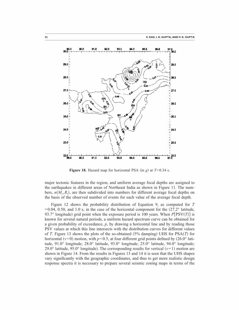
Figure 18. Hazard map for horizontal PSA �in g� at T=0.34 s.
A PROBABILISTIC SEISMIC HAZARD ANALYSIS OF NORTHEAST INDIA 23
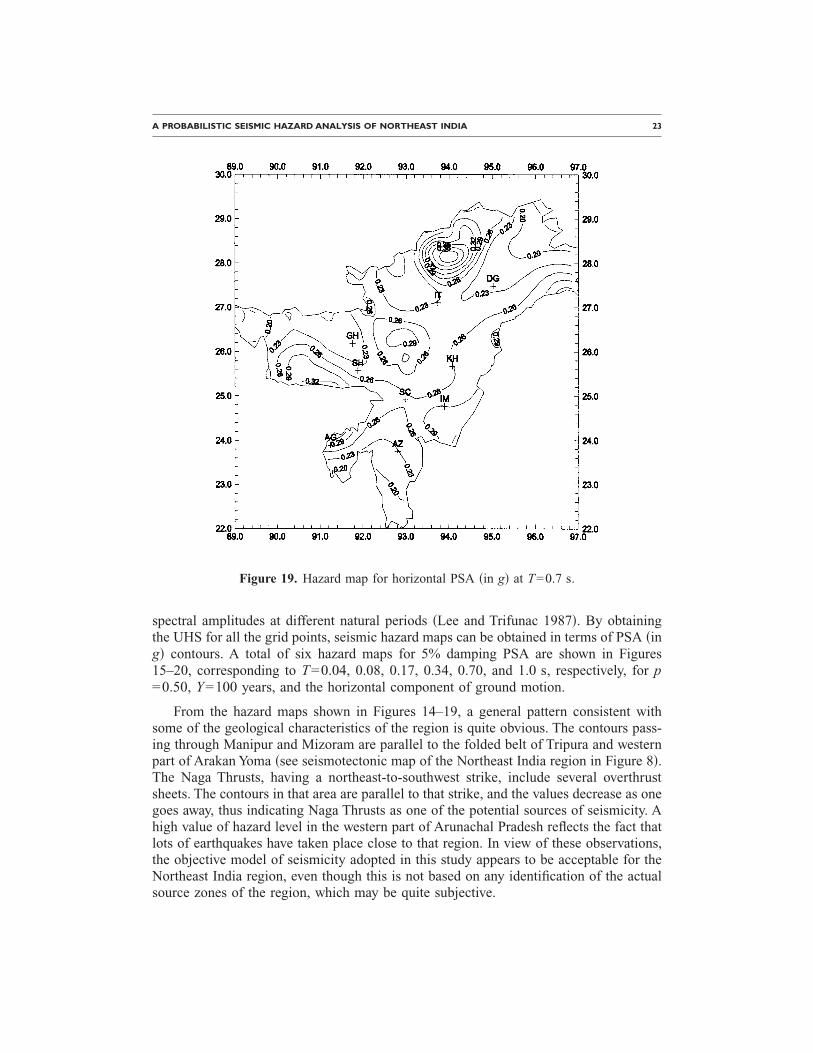
spectral amplitudes at different natural periods �Lee and Trifunac 1987�. By obtainingthe UHS for all the grid points, seismic hazard maps can be obtained in terms of PSA �ing� contours. A total of six hazard maps for 5% damping PSA are shown in Figures15–20, corresponding to T=0.04, 0.08, 0.17, 0.34, 0.70, and 1.0 s, respectively, for p=0.50, Y=100 years, and the horizontal component of ground motion.
From the hazard maps shown in Figures 14–19, a general pattern consistent withsome of the geological characteristics of the region is quite obvious. The contours pass-ing through Manipur and Mizoram are parallel to the folded belt of Tripura and westernpart of Arakan Yoma �see seismotectonic map of the Northeast India region in Figure 8�.The Naga Thrusts, having a northeast-to-southwest strike, include several overthrustsheets. The contours in that area are parallel to that strike, and the values decrease as onegoes away, thus indicating Naga Thrusts as one of the potential sources of seismicity. Ahigh value of hazard level in the western part of Arunachal Pradesh reflects the fact thatlots of earthquakes have taken place close to that region. In view of these observations,the objective model of seismicity adopted in this study appears to be acceptable for theNortheast India region, even though this is not based on any identification of the actualsource zones of the region, which may be quite subjective.
Figure 19. Hazard map for horizontal PSA �in g� at T=0.7 s.

24 S. DAS, I. D. GUPTA, AND V. K. GUPTA
It may be mentioned that the proposed hazard maps are specifically for the stiff sites�firm ground or sedimentary rock�, due to the data used in the development of underly-ing attenuation model. Thus the information available from these maps may need furtherprocessing for use in case of medium to soft soil deposits at a site.
SUMMARY AND CONCLUSIONS
A probabilistic seismic hazard analysis based on the uniform hazard spectra for PSVhas been carried out in Northeast India. For this purpose, a spectral attenuation modelhas been developed by using a total of 261 accelerograms recorded at different stationson stiff sites in the region. The proposed model is able to capture the frequency-dependent variations in PSV, and properly accounts for the effects of earthquake mag-nitude, epicentral distance, and focal depth on the PSV spectral shapes, for both hori-zontal and vertical motions. A regionalization-free approach has then been proposed todefine the seismicity model of the region of interest. This approach is based on the dataof past earthquake events over a long period of time from 1458 to 2000. In this ap-proach, the entire region is divided into a fine grid of around 2,500 nodes, and hazardlevel is predicted for each of the nodes by assuming it to be dependent on the earthquake
Figure 20. Hazard map for horizontal PSA �in g� at T=1.0 s.

A PROBABILISTIC SEISMIC HAZARD ANALYSIS OF NORTHEAST INDIA 25
events within a 300-km-radius area. The number of events expected to occur in differentmagnitude classes is obtained from the G-R relationship conforming to the data of pastearthquake events. Using the spatial distribution of past earthquakes, these are then dis-tributed among 50 source elements, with each source element assumed to be represent-ing an annular-shaped area around the node of interest. Even though actual seismotec-tonic source zones are not identified in this approach, the estimated hazard mapping isfound to be consistent with the main tectonic features in the northeast region.
Seismic hazard maps for 50% confidence level and ten natural periods between 0.04and 1.0 s have been presented in terms of 5% damping PSA contours on stiff grounds.These maps provide much more detailed and direct information about the seismic hazardthan those based on the use of PGA together with a standard spectral shape.
REFERENCES
Anderson, J. G., and Trifunac, M. D., 1977. On Uniform Risk Functionals Which DescribeStrong Earthquake Ground Motion: Definition, Numerical Estimation, and an Application tothe Fourier Amplitude of Acceleration, Report CE 77-02, University of Southern California,Los Angeles, CA.
Anderson, J. G., and Trifunac, M. D., 1978. Uniform risk functionals for characterization ofstrong earthquake ground motion, Bull. Seismol. Soc. Am. 68, 205–218.
Bapat, A., Kulkarni, R. C., and Guha, S. K., 1983. Catalogue of Earthquakes in India andNeighbourhood from Historical Period up to 1979, Indian Society of Earthquake Technol-ogy, Roorkee, India.
Basu, S., and Nigam, N. C., 1978. On seismic zoning map of India, Proceedings, VI Symposiumon Earthquake Engineering, Roorkee, India, Vol. I, pp. 83–90.
Bernreuter, D. L., Savy, J. B., Mensing, R. W., and Chen, J. C., 1989. Seismic Hazard Charac-terization of 69 Nuclear Power Plant Sites East of the Rocky Mountains, NUREG/CR-5250,U.S. Nuclear Regulatory Commission.
Bhatia, S. C., Ravikumar, M., and Gupta, H. K., 1999. A probabilistic seismic hazard map ofIndia and adjoining regions, Annali Di Geofisica 42 �6�, 1153–1164.
Chandrasekaran, A. R., and Das, J. D., 1993. Strong Earthquake Ground Motion Data in EQIN-FOS for India: Part 1B, Univ. of Roorkee and Univ. of Southern California, Dept. of CivilEng., Report No. CE93-04, edited by M. D. Trifunac, M. I. Todorovska, and V. W. Lee.
Cornell, C. A., 1968. Engineering seismic risk analysis, Bull. Seismol. Soc. Am. 58, 1583–1606.
Douglas, J., 2001. A Comprehensive Worldwide Summary of Strong-Motion Attenuation Rela-tionships for Peak Ground Acceleration and Spectral Ordinates �1969 to 2000�, ESEE Re-port No. 01-1, Imperial College of Science, Technology and Medicine, Civil Eng. Dept.,London, U.K.
Douglas, J., 2002. Errata of and addition to ESEE Report No. 01-1.
Electric Power Research Institute �EPRI�, 1986. Seismic Hazard Methodology for the Centraland Eastern United States, Report NP-4726, Palo Alto, CA.
Frankel, A., 1995. Mapping seismic hazard in the central and eastern United States, Seismol.Res. Lett. 66 �4�, 8–21.
26 S. DAS, I. D. GUPTA, AND V. K. GUPTA
Gupta, I. D., 2002. Should normalised spectral shapes be used for estimating site-specific de-sign ground motion? Proceedings, 12th Symposium on Earthquake Engineering, Roorkee,Vol. I, pp. 168–175.
Gutenberg, B., and Richter, C. F., 1944. Frequency of earthquakes in California, Bull. Seismol.Soc. Am. 34, 185–188.
Joyner, W. B., and Boore, D. M., 1981. Peak horizontal acceleration and velocity from strongmotion records including records from the 1979 Imperial Valley, California, earthquake,Bull. Seismol. Soc. Am. 71 �6�, 2011–2038.
Kaila, K. L., and Rao, N. M., 1979. Seismic zoning maps of Indian subcontinent, Geophys. Res.Bull. 17, 293–301, National Geophysical Research Institute, Hyderabad, India.
Khattri, K. N., Rogers, A. M., and Algermissen, S. T., 1984. A seismic hazard map of India andadjacent areas, Tectonophysics 108, 93–134.
Lee, V. W., 1992. On strong motion risk functionals computed from general probability distri-butions of earthquake recurrence, Soil Dyn. Earthquake Eng. 11, 357–367.
Lee, V. W., 2002. Empirical scaling of strong earthquake ground motion—Part I: Attenuationand scaling of response spectra, ISET J. Earthquake Technol. 11 �4�, 219–254.
Lee, V. W., and Trifunac, M. D., 1979. Automatic Digitization and Processing of Strong MotionAccelerograms, Report No. CE79-15 I and II, Univ. of Southern California, Dept. of CivilEng., Los Angeles, CA.
Lee, V. W., and Trifunac, M. D., 1987. Microzonation of a Metropolitan Area, Report No.CE87-02, Univ. of Southern California, Dept. of Civil Eng., Los Angeles, CA.
McGarr, A., 1984. Scaling of ground motion parameters, state of stress, and focal depth, J.Geophys. Res. 89, 6969–6979.
Orozova, I. M., and Suhadolc, P., 1999. A deterministic-probabilistic approach for seismic haz-ard assessment, Tectonophysics 312, 191–202.
Peruzza, L., Slejko, D., and Bragato, P. L., 2000. The Umbria-Marche case: Some suggestionsfor the Italian seismic zonation, Soil Dyn. Earthquake Eng. 20, 361–371.
Senior Seismic Hazard Analysis Committee �SSHAC�, 1997. Recommendations for Probabilis-tic Seismic Hazard Analysis: Guidance on Uncertainty and Use of Experts, NUREG/CR-6372, U.S. Nuclear Regulatory Commission.
Stepp, J. C., 1973. Analysis of completeness of the earthquake sample in the Puget Sound area,in Seismic Zoning, edited by S. T. Harding, Report ERL 267-ESL30, NOAA Tech, Boulder,CO.
Todorovska, M. I., 1994. Comparison of response spectrum amplitudes from earthquakes withlognormally and exponentially distributed return period, Soil Dyn. Earthquake Eng. 13 �2�,97–116.
Todorovska, M. I., Gupta, I. D., Gupta, V. K., Lee, V. W., and Trifunac, M. D., 1995. SelectedTopics in Probabilistic Seismic Hazard Analysis, Report No. CE95-08, Dept. of Civil Eng.,Univ. of Southern California, Los Angeles, CA.
Trifunac, M. D., 1971. Zero base-line correction of strong-motion accelerograms, Bull. Seismol.Soc. Am. 61 �5�, 1201–1211.
Trifunac, M. D., 1972. A note on correction of strong-motion accelerograms for instrument re-
sponse, Bull. Seismol. Soc. Am. 62 �1�, 401–409.
A PROBABILISTIC SEISMIC HAZARD ANALYSIS OF NORTHEAST INDIA 27
Trifunac, M. D., 1980. Effects of site geology on amplitudes of strong motion, Proceedings, 7thWorld Conference on Earthquake Engineering, Vol. 2, pp. 145–152.
Trifunac, M. D., 1990. A microzonation method based on uniform risk spectra, Soil Dyn. Earth-quake Eng. 9 �1�, 34–43.
Trifunac, M. D., 1992. Should peak acceleration be used to scale design spectrum amplitude?Proceedings, 10th World Conference on Earthquake Engineering, Madrid, Spain, Vol. 10, pp.5817–5822.
Trifunac, M. D., and Lee, V. W., 1989. Empirical models for scaling pseudo relative velocityspectra of strong earthquake accelerations in terms of magnitude, distance, site intensity andrecording site conditions, Soil Dyn. Earthquake Eng. 8 �3�, 126–144.
Trifunac, M. D., and Lee, V. W., 1990. Frequency-dependent attenuation of strong earthquakeground motion, Soil Dyn. Earthquake Eng. 9 �1�, 3–15.
Veneziano, D., Cornell, C. A., and O’Hara, T., 1984. Historic Method for Seismic HazardAnalysis, Report NP-3438, Electric Power Research Institute, Palo Alto, CA.
Verma, R. K., Mukhopadhyay, M., and Ahluwalia, M. S., 1976. Seismicity, gravity, and tecton-ics of Northeast India and Northern Burma, Bull. Seismol. Soc. Am. 66 �5�, 1683–1694.
Wahlström, R., and Grünthal, G., 2001. Probabilistic seismic hazard assessment �horizontalPGA� for Fennoscandia using the logic tree approach for regionalization and nonregional-ization models, Seismol. Res. Lett. 72 �1�, 33–45.
Weichert, D. H., 1980. Estimation of earthquake recurrence parameters for unequal observa-tional periods for different magnitudes, Bull. Seismol. Soc. Am. 70, 1337–1346.
Wheeler, R. L., and Mueller, C. S., 2001. Central U.S. earthquake catalog for hazard maps ofMemphis, Tennessee, Eng. Geol. 62, 19–29.
Woo, G., 1996. Kernel estimation methods for seismic hazard area source modeling, Bull. Seis-mol. Soc. Am. 86, 353–362.
�Received 25 April 2004; accepted 2 May 2005�