A Simple and Unified Method for Drawing Graphs: Magnetic-Spring Algorithm

Kozo Sugiyama and Kazuo Misue

Institute for Social Information Science, Fujitsu Laboratories Limited 140 Miyamoto, Numazaa, Shizuoka, 410-03, JAPAN

{sugi, misue } @iias.flab. fujitsu.co.jp

A simple and unified heuristic method for nicely drawing directed, undirected and mixed graphs is proposed basing upon a new model called magnetic.spring model which is an extension of Eades's spring model. In the new model, the idea of controlling edge orientations by magnetic forces is employed. Since the method is conceptually intuitive, it is quite easy to understand, implement, tune and improve it. Examples of layouts and results of experiments are shown to demonstrate extensive possibilities of the method.

1 Introduction

Force-directed placement is a well-known technique for drawing general undirected graphs[I,2,3,4]. As one of the early works of the force-directed placement, Eades[2] presented an algorithm based upon the spring model. In the model, vertices are replaced with steel rings and each edge with a spring to form a mechanical system, and repulsive and attractive forces are defined among rings. Then the rings are placed in some initial layout and moved iteratively according to the forces so that the system reaches a minimal energy state. Finally rings are drawn as points or small circles, and each edge as a straight line segment between a pair of rings connected by the edge. Kamada[3] proposed a more sophisticated algorithm and Fruchterman & Reingold[4] presented an effective modification of the model.

Aesthetic criteria generally accepted in the force-directed placement approach have been[4]: uniforming edge lengths (A1), minimizing edge crossings (A2), revealing symmetry (A3), distributing vertices evenly (A4) and conforming to the frame (A5). In this paper we introduce a new aesthetic criterion, i.e. conforming edges to specified orientations (A6), and propose a method based on a new model called magnetic-spring model. In this model, as shown in Fig.l, vertices are replaced with rings and edges with magnetic springs, and various types of magnetic fields are introduced. With this model we can not only obtain the placement of vertices satisfying the generally accepted criteria, but also Can control the geometrical orientations of edges by magnetic rotative forces. This can provide us with novel capabilities in graph drawing by force-directed placement: This method can draw, in a simple and unified manner, not only undirected graphs but also trees, directed graphs and mixed graphs (graphs with both directed and undirected edges). Moreover, since this method is based upon the idea of simulations of virtual physical systems, it is conceptually intuitive and quite easy to be understood, implemented, tuned and modified. Therefore, this method might be useful for non-expert users who want to visualize graphs flexibly with a drawing tool made by themselves even if the visualization is approximate.

Fig.2 shows an example of mixed graph appeared in the literature[5]. This is an issue map in which four types of relationships are used: One of them is uni-

+ i

directional and the rest three are bi-directional. How to control the orientations of these edges and draw the graph is a quite interesting problem. However, such the problem has not been considered so far. Our method is specially suitable for drawing complicated graphs like the mixed graph shown in Fig.2.

In the second section a magnetic-spring model is presented. In the third section several experiments for showing the possibilities of our method are carried out. Experimental results and discussions are shown along seven questions raised on the ability of our method by the authors. Finally concluding remarks are made with suggestions for future research.

MF SF

St~etic~A_~

magnetic field

J M

MF

RF

RSF

Fig.1. Magnetic-spring model. ASF: at~active spring force, RSF: repulsive spring force, RF: repulsive force and MF: magnetic force.

/

365

AssoclJte

~ e p e n d r issues

C ~ e d issu~ from bt+~.-d to specific

Contradictory issues

Fig.2. An example of a mixed graph: art issue map.

2 Model and Algorithm

In developing a new method, we adopt three principles for graph drawing: (1) Vertices connected by an edge should be drawn near each other; (2) Vertices should not be drawn too close to each other; and (3) Different types of edges should be drawn with different specified orientations.

366

The f'trst two principles are just same as those of Eades[2] and Furuchterman & Reingold[4], and the last is our new principle.

2.1 Magnetic-Spring Model

A graph G =(V, E ) consists of a set V of vertices and a set E of pairs of vertices. An element of E is called an edge. A graph G =(V, E ) is modeled as follows. The model does not reflect the natural reality readily or is characterized as a virtual model as well as the spring model.

Rings and Springs

Every vertex in V is replaced with a steel ring as shown in Fig.1. Edges in E are classified into magnetic edges and non-magnetic edges. Magnetic edges are replaced with magnetic springs and non-magnetic edges with springs. Magnetic springs consist of uni-directional magnetic springs and bi-directionai magnetic springs as shown in Fig.3. Usually directed edges are assigned as magnetic edges and replaced with uni-directional magnetic springs. Undirected edges are usually assigned as non-magnetic edges but sometimes they are assigned as magnetic edges and replaced with bi-directional magnetic springs. How to assign such the magnetic property of edges substantially depends on applications.

m tn

02 ~ ~

Fm

Fig.3. Uni-directional spring (left) and bi-directional spring (right), and magnetic forces.

Fields

We consider three types of standard magnetic fields: parallel, polar and concentric; and two types of compound magnetic fields: orthogonal and polar-concentric (see Fig.4). Compound magnetic fields are composed from standard magnetic fields. When we put b(x,y) and m(x,y ) as the strength of a magnetic field and the orientation vector that expresses the orientation of the field at any point (x,y) respectively, each standard magnetic field B (x,y) at (x, y) is given by

(x,y) = b re(x, y) . (1)

367

In this paper we consider uniform fields for simplicity and therefore we put b is constant at any point (x ,y) except the origin(0, 0); specially B (0, 0) = 0 in the cases of polar and concentric fields. We put m (x, y ) as follows:

(1) parallel field

m ( x , y ) = (0, 1):north; (-1,0):west; (0,-1):south; (1,0):east. (2)

(2) polar field

m (x, y ) = (x , y )/l(x , y )l. (3)

(3) concentric field

m (x, y ) = (y , -x )/l(x, y )1 : clockwise; (-y, x )/l(x, y )1 : anti-clockwise. (4)

(a)

I - I ->

--h-

(d)

(b) (c)

(e)

Fig.4. Standard and compound magnetic fields: (a) parallel, (b) polar, (c) concentric, (d) orthogonal and (e) polar-concentric.

Forces

We consider three types of forces (see Fig.3): (1) F s : attractive or repulsive forces exerted by the springs between neighbors; (2) Fr : repulsive forces between every pair of non-neighboring vertices; and (3)Fro : rotative forces exerted on edges by the magnetic field.

The ideas of the first two forces are based on Eades's model. The last is calculated as forces exerted on the vertices connected by each magnetic edge. Strengths of these forces are given by:

368

F~ = c~ log(e/k) (5)

Fr = -Cr 1/d 2 (6)

Fm = c m b d a O [J (7)

where d is the distance between a pair of vertices, k is an ideal distance between neighbors, 0 (-x < 0 < ~ ) is the angle (radian) from the orientation of the field to the orientation of the magnetic edge, and a, fl, cs, Cr, cm > 0 are parameters for tuning the model. In the case of a bi-directional magnetic edge, there can exist two angles 01(negative) and 02 (positive). We select for 0 the one of which absolute value is smaller than the other. Though magnetic forces Fm are exerted on each magnetic edge by a magnetic field, we calculate them as two forces (with a same strength and reverse orientations) exerted on a pair of vertices connected by the edge.

Anchors

We introduce special rings called anchor rings which never be moved even if some force is exerted on the rings. We can extend the idea of anchor rings to anchor bars and anchor frames, but we do not use them in this paper.

2.2 Algorithm

Our algorithm is based upon Eades's algorithm[2] in which the mechanical system is simulated. Before starting calculations we should specify natures of forces as F, a type of magnetic field as M and types of edges in terms of magnetic responses as R.

algorithm MAGNETIC_SPRING (G : graph, F : natures of forces, M : a type of magnetic field, R : specifications of magnetic responses);

1. place vertices of G on a circle evenly, of which radius is k IV I/2n, in a random order;

2. repeat n times 2.1 calculate the force exerting on each vertex by composing three kinds of

forces according to F, M, R ; 2.2 move each vertex by 8 x (force on the vertex);

3. draw the graph on a screen.

Parameter 8 controls the magnitude of moving steps. Calculations of forces Fs's, Fr's and Fin's have O(IEI ), O(IVI 2) and O(IEI] time complexity respectively. An initial placement of vertices on a circle can be seen in Fig.5a.

3 S u m m a r y o f E x p e r i m e n t s

In this section, we show a brief summary of experiments to check the usefulness of controlling edge orientations and test the capabilities of our method. A more detailed

369

version can be seen in [6]. In the experiments we randomly generate thirty sample graphs, all of which are connected, for various cases such as:

(1) classes of graphs: rooted trees (RT), acyclic directed graphs (ADG), cyclic directed graphs (CDG), edge-bipartite rooted trees (EBRT) and acyclic mixed graphs (AMG);

(2) the number of vertices: 20 and 40; (3) mean degree: 2.5 and 3.0 (nearly 2 in the case of tree).

Then we apply our algorithm to the sample graphs in various magnetic fields shown in Fig.4 and calculate the five quantitative values that relate to the several aesthetic criteria: the number of crossings(A2), the distribution of angles between edge- orientations(A6), the number of error edges of which orientations do not conform to the magnetic field(A6), the distribution of edge lengths(A1) and the density of vertices distribution(A4). In the experiments default values of parameters are set as r ~--1.0, Cs~2.0, Cr =1.0, Cra=l.O and k=l.0. Parameter b is changed between 0.0 and 16.0 to observe effects due to the strength of a magnetic field. Parameter 8is changed between 0.005 and 0.1 so that the larger b is, the smaller 8 is, which is to make the length of a moving step equal through simulations. Therefore the number of steps diverges from 100 to 1600. In investigating the performance, our interests exists in the following questions.

(Q1) Can rooted trees be drawn without crossings or with a few crossings?

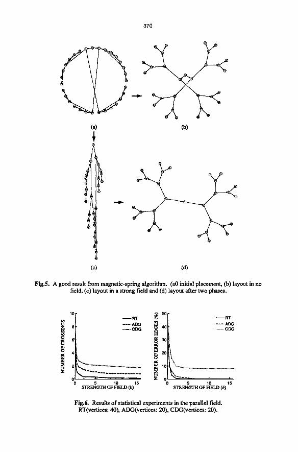
Both Eades[7] and Fruchterman & Reingold[4] reported the difficulty of drawing trees without edge crossings by spring algorithms. However, we can overcome it and obtain a good layout by using our magnetic-spring algorithm. Fig.5a shows an initial placement of the graph. If there does not exist any magnetic field, we obtain the layout shown in Fig.5b where we can not eliminate a crossing, whereas if there exists a suong parallel field, we obtain the crossing-free layout shown in Fig.5c. Fig.5c is laid out in a tree form, but the diagram is too narrow due to the existence of the strong field. Therefore, we further continue the calculation in no magnetic field as the next phase and then we get the symmetrical layout presented in Fig.5d. Thus this two-phase algorithm is quite effective to obtain good layouts of rooted trees. The good performance to reduce the number of crossings in drawing rooted trees by our algorithm is also confirmed from statistical experiments. Fig.6 shows a part of the experimental results in a parallel field where for rooted trees the expected number of crossings is very low and every edge conforms to the orientation of the field when the strength of the field is high.

(Q2) Can downward (or upward) drawings of acyclic directed graphs be easily realized?

With the magnetic-spring algorithm we can realize easily downward (or upward) layouts of acyclic directed graphs. Fig.7 shows layouts of an acyclic directed graph when the strength of the magnetic field is changed. Fig.7a corresponds to the case of no magnetic field and Fig.7c the strongest. We can see from Fig.6 that for acyclic directed graphs there is no error edge when the magnetic force is strong.

(Q3) How about relationships between our method and the feedback edge set problem in the case of drawing cyclic directed graphs?

370

(a) (b)

(c) (d)

Fig.5. A good result from magnetic-spring algorithm. (a0 initial placement, (b) layout in no field, (c) layout in a strong field and (d) layout after two phases.

10

,v 6 U

0

0 0

.... ACN3 --- AEX~

........ COG ....... CDG

== 30 =o

'If , . ~ 0 I- ~ . . . . . ,

5 10 15 0 5 10 15 STRENGTH OF F IELD (b) S T R E N G T H OF FIT~LD (b)

Fig.6. Results of statistical experiments in the parallel field. RT(v,e~ices: 40), ADG(vertices: 20), CDG(ve~ices: 20).

371

What is most interesting in drawing cyclic directed graphs in a parallel field is whether the number of feedback edges is close to minimal or not. Fig.8 displays a good example from our algorithm. In Fig.8c only one edge (0---)4) is pointing upward whereas all other edges downward. This means that the minimum feedback edge set problem is solved. Of course, this can not be confirmed by statistical experiments in general. However, the number of feedback edges (or error edges) is small (about 10% of IEI) in the parallel field as seen in Fig.6.

V

(a) b = 0 (b )b= 1 (c) b = 4

Fig.7. Layouts of an acyclic directed graph in the parallel field.

(a) b = 0 (d) b = 2 (f) b = 8

Fig.8. Layouts of a cyclic directed graph in the parallel field.

(Q4) Is our method effective for h-v drawing of rooted binary trees?

Fig.9 shows layouts of edge-bipartite rooted trees that represent h-v drawings[8] of a list structure where car-edges are drawn vertically and cdr-edges horizontally. An edge-bipartite rooted tree is placed in an orthogonal field and its layouts are calculated changing the slrength of the field. Though there is no crossing in Fig.9a, we can not always eliminate crossings even if we use the two-phase algorithm. Fig.9b shows an example of a larger rooted tree where the orientations of edges conform

372

(a) (b) Fig.9. Layouts of an edge-bipartite rooted tree in the orthogonal field.

10

6

4

0 0

EBRT ~, 50

. . . . AMG ~ 40

nr 30

' ' ' ' ' ' ' ' ' ' ' ' ' ' ' ' ' ' i '10

I |' / 0 5 10 15 0

STRENGTH OF FIELD (b)

~ E B R T . . . . AMG

5 10 15 STRENGTH OF FIELD (b)

Fig.10. Results of statistical experiments in the orthogonal field. EBRT(vertices: 20), AMG(vertices: 20).

well to the field but there remain several crossings. A part of results of statistical experiments for each case is shown in Fig.10.

(Q5) Can acyclic mixed graphs be drawn in a way that we can easily grasp a global structure constituted with different kinds of edges and distinguish them readily?

In the acyclic mixed graph presented in Fig.2 where there is no directed cycle, uni- directional relationships are replaced with uni-directional magnetic springs and three types of bi-directional relationships all are replaced with bi-directional magnetic springs. Then our algorithm is applied to the graph so that the former relationships are drawn downward and the latter horizontally as much as possible. Fig.11 shows variations of diagrams of the acyclic mixed graph where we can distinguish uni- directional relationships from bi-directional relationships more easily in the case of the strong field than in the case of no field. A part of results of statistical experiments are shown in Fig.10.

(Qt) To which kind of problems is a polar field applicable?

373

":L i

�9 :.$ ........

~176176

- - -~ .2~" '~

( a ) b = O Co) b = 4

Flg.ll. Layouts of an aeyclic mixed graph(Fig.2) in the orthogonal field.

Reggiani and Marchetti[9] found that if a vertex-bipartite graph was drawn as a hierarchy with two horizontal levels then its diagram could not avoid many crossings (see Fig. 12a), whereas if it was drawn as a hierarchy with two concentric discs then its diagram could avoid crossings completely (see Fig. 12b). In order to check this ability of our algorithm, we place the same graph in the polar field and apply our algorithm to it where an anchor vertex connecting to vertices with numeric labels is placed at the origin. Fig.12c is a resulted diagram where the orientation of every edge conforms to the orientation of the field, but three crossings can not be eliminated.

h ." ! 5 '" ,

: " [

a b c d e f g h b

(a) 0~) (c)

Fig.12. Layouts of a vertex-bipartite graph by several drawing methods.

(Q7) Can cyclic directed graphs be drawn in a way that it is easy to grasp the global flow of the graphs and the existence of cycles?

Fig.13 shows variations of layouts of cyclic directed graphs obtained from our algorithm when the strength of a concentric field is changed. Figs.13a (tetragonal pillar) and 13b (.pentagonal pillar) correspond to the cases of no field and Figs.13a' and 13b' the strongest. When we increase the field strength, we can obtain symmetrical layouts where the conformity to the orientation of the field is attained, which bring us the easiness for grasping cycles. We check whether this advantage of

374

(a) b = 0 (b) b = 0 (c) b = 0

(a3 b =1 (b3 b ffi 1 (e3 b = 8

Fig.13. Layouts of three cyclic directed graph in the concentric field.

10

r~

6

4

2

0

50

~ C D G ~ 40

, , ; 5 10 1 0

STRENGTH OF F l ~ . n (b)

~ C D G

' o ' 5 1 15 STRENGTH OF FIELD (b)

Fig.14. Results of statistical experiments in the concentric field.

our algorithm arises even for more general cases. Figs.13c and 13c' shows variations of layouts of a more general cyclic directed graph (same graph as Fig.8) where we can recognize cycles easily when the field becomes strong. A part of results of statistical experiments are shown in Fig. 14.

375

4. Concluding Remarks

Since the magnetic-spring method is substantially heuristic, we can not give exact answers to the above-stated problems. However, the results of preliminary experiments presented in the paper show extensive possibilities of the method, especially in problems like (Q1), (Q2), (Q4), (Q5) and (Q7). Also, since this method is very simple and applicable to the wide range of graphs, the method might be suitable for non-expert users who want to visualize graphs flexibly with a drawing tool made by themselves even if the visualization is approximate. Interactive environments are desirable for raising the flexibility of the algorithm.

For future research it is envisaged to analyze more precisely trade-off relationships among aesthetic criteria, diversify the idea of fields, extend virtual models and sophisticate formulations and algorithms in both theoretical and practical senses.

References

[1IN. Quinn and M. Breur: A force directed component placement procedure for printed circuit boards, IEEE Trans. Circuits and Systems, CAS-26(6), 377-388, (1979). [2] P. Eades: A heuristic for graph drawing, Congressus Numerantium 42, 149-160, (1984). [3] T. Kamada: On visualization of abstract objects and relations, Dr. S. thesis, Univ. of Tokyo, (1988). [4] T. Fruchterman and E. Reingold: Graph drawing by force-directed placement, Software - Practice and Experience 21(11), 1129-1164, (1991). [5] M. J. Bickerton: A practitioner's handbook of requirement engineering methods and tools, Oxford Univ., (1992). [6] K. Sugiyama and K. Misue: Graph Drawing by Magnetic-Spring Model, Res. Rep. ISIS-RR-94-14E, Inst. Social Information Science, Fujitsu Labs. Ltd., 32p., (1994). [7] P. Eades: Drawing free trees, Res. Rep. IIAS-RR-91-17E, Intern. Inst. for Advanced Study of Social Information Science, Fujitsu Lab. Ltd., 29p., (1991). [8] P. Creszenzi, G. Di Battista and A. Piperno: A note on optimal area algorithms for upward drawings of binary trees, J. Computational Geometry, 2(4), 187-200, (1992). [9] M. G. Reggiani and F. E. Marchetti: A proposed method for representing hierarchies, IEEE Trans. Systems, Man, and Cybernetics SMC-18(1), 2-8, (1988).