a stable self-structuring adaptive fuzzy control …. (mechatronics eng., hons.) ... chapter 1...
TRANSCRIPT

A Stable Self-Structuring Adaptive
Fuzzy Control Scheme for Continuous
Single-Input Single-Output Nonlinear
Systems
by
Phi Anh Phan
B.Eng. (Mechatronics Eng., Hons.)
Submitted in fulfilment of the requirements for the Degree of Doctor of Philosophy
School of Engineering, University of Tasmania
March 2009

2
Statement of Originality & Authority of Access
This thesis contains no material which has been accepted for a degree or diploma
by the University of Tasmania or any other institution, except by way of background
information and has been duly acknowledged in this thesis, and to the best of the
author’s knowledge and belief no material has previously been published or written
by another person except where due acknowledgement is made in the text of this
thesis.
This thesis contains confidential information and is not to be disclosed or made
available for loan or copy without the expressed permission of the University of
Tasmania. Once released the thesis may be made available for loan and limited
copying in accordance with the Copyright Act 1968.
School of Engineering,
University of Tasmania,
Hobart, Tasmania, Australia

3
Abstract
Adaptive fuzzy control has been an active research area in the past decade.
Fundamental issues such as stability, robustness, and performance analysis have been
solved. However, one main drawback is the generally fixed structure of the fuzzy
controllers, which are normally chosen by trial-and-error in practice. Few attempts to
develop self-structuring AFC have been reported, and important issues such as
stability, computational efficiency, and implementability have not been investigated
thoroughly. In particular, the stability of the system when the structure changes has
not been proven. Thus, a more effective self-structuring AFC scheme is desirable.
The main objective of the research is to develop a stable self-structuring AFC
scheme for continuous-time single-input-single-output (SISO) uncertain nonlinear
systems.
A novel online self-structuring adaptive fuzzy control scheme that is applicable
for a number of classes of continuous SISO nonlinear systems is proposed. The
applicable classes include affine nonlinear systems, non-affine nonlinear systems, and
nonlinear systems in triangular forms. The main features of the proposed control
scheme are:
• It needs less restriction on the controlled plants and no restriction on the
design parameters.
• It employs a modified adaptive law that guarantees explicit boundedness of
adaptive parameters and control action.
• The self-structuring algorithm is relatively simple and guarantees explicit
boundedness of the number of rules generated.
• Only triangular membership functions are generated and only 2
membership functions are allowed to overlap to increase the
interpretability of generated fuzzy controllers.
• High-gain observers are used when not all the states are measurable and
the design of observers is completely separated from the design of
controllers.
• For nonlinear systems in triangular forms, only one fuzzy system is needed
(unlike the back-stepping approach where one fuzzy system is needed at
each step).
4
• An approximation error estimator and an automatic switching mechanism
can be used to further increase the robustness and computational
efficiency.
The stability of the overall system, especially when the structure changes, is
guaranteed using the Lyapunov stability technique. The overall system is stable in the
sense that all the variables are bounded (including number of rules generated) and the
tracking error is uniformly ultimately bounded. The proposed control algorithms are
implemented in Matlab and Simulink for ease of simulation and practical application.
Numerous simulation examples are performed to demonstrate the theoretical results.
The proposed control scheme makes practical application of AFC easier.
Designers need to specify only a few design parameters and no longer have to specify
the controller structure by trial and error. A simulation or application can be quickly
and easily implemented using the developed controllers in Simulink.
Publications
As part of this research, the following papers have been published:
Journal papers:
• P.A. Phan, and T.J. Gale, “Two-mode adaptive fuzzy control with approximation error estimator”, IEEE Transactions on Fuzzy Systems, volume 15 (5), pp 943-955, Oct. 2007.
• P.A. Phan, and T.J. Gale, “Direct adaptive fuzzy control with less restrictions on the control gain”, International Journal of Control, Automation, and Systems, Vol 5 No 6 Dec 2007, in press.
• P.A. Phan, and T.J. Gale, “Direct Adaptive Fuzzy Control with a Self-Structuring Algorithm”, Fuzzy Sets and Systems, in press.
Conference papers:
• P. A Phan, and T.J. Gale, ‘Stable Adaptive Fuzzy Controller with Approximation Error Estimators’, Proceedings of The 2nd International Conference on Artificial Intelligence in Science and Technology, Hobart, Tas. Australia, 295-300 (2004)
• P.A. Phan, and T.J. Gale, “Adaptive fuzzy control: approximation error estimator approach”, 23rd IASTED
International Conference on Artificial Intelligence and Applications, Innsbruck, Austria, 2005.
• P.A. Phan, and T.J. Gale, “Direct adaptive fuzzy control with less restrictions on the control gain”, International Conference on Computational Intelligence for Modelling, Control, and Automation, Sydney, Australia, 2006.

5
Acknowledgements
I would like to thank my supervisor, Dr. Timothy J Gale, for his endless
guidance, support and friendship throughout the duration of the research. He was
always there whenever I needed help.
I would also like to thank my associate supervisors, Dr. Bernardo A Leo de La
Barra and Prof Michael Negnevitsky, for their advices and help in Control and
Artificial Intelligence.
Most importantly, I would like to thank my family for their love and support.
Without them, I would not have completed this project.
Finally, I would like to thank all my friends who have helped and assisted me
during my time at University of Tasmania.
6
Table of Contents
ABBREVIATIONS.................................................................................................................................9
1. CHAPTER 1 INRODUCTION ..................................................................................................10
1.1. INTRODUCTION .....................................................................................................................10 1.2. ADAPTIVE FUZZY CONTROL ..................................................................................................10
1.2.1. What is adaptive fuzzy control? ......................................................................................11 1.2.2. Why adaptive fuzzy control? ...........................................................................................11 1.2.3. Relationship between adaptive fuzzy control and adaptive neural network control .......13
1.3. MOTIVATION AND OBJECTIVES ............................................................................................13 1.4. OUTLINE OF THE THESIS .......................................................................................................14 1.5. CONCLUSION ........................................................................................................................16
2. CHAPTER 2 GENERAL LITERATURE REVIEW AND PRELIMINARIES....................17
2.1. INTRODUCTION .....................................................................................................................17 2.2. A REVIEW ABOUT THE DEVELOPMENT OF ADAPTIVE FUZZY CONTROL..................................17
2.2.1. Structure..........................................................................................................................17 2.2.1.1. Direct AFC ..........................................................................................................................17 2.2.1.2. Indirect AFC........................................................................................................................18 2.2.1.3. AFC combined with other controllers .................................................................................18
2.2.2. Different classes of nonlinear systems ............................................................................20 2.2.2.1. Affine and non-affine nonlinear systems.............................................................................20 2.2.2.2. Strict-feedback and pure-feedback nonlinear systems.........................................................22 2.2.2.3. SISO and MIMO nonlinear systems....................................................................................24 2.2.2.4. State-feedback and output feedback nonlinear systems.......................................................25 2.2.2.5. Continuous and discrete systems .........................................................................................25
2.2.3. Adaptive mechanism of fuzzy systems .............................................................................26 2.2.3.1. Only parameters are tuned...................................................................................................26 2.2.3.2. Both parameters and structure are adjusted .........................................................................26
2.3. PRELIMINARIES.....................................................................................................................27 2.3.1. Fuzzy system and neural network ...................................................................................27 2.3.2. Concepts of stability and boundedness ...........................................................................27
2.3.2.1. Stability definitions .............................................................................................................28 2.3.2.2. Boundedness definitions......................................................................................................29
2.3.3. Lyapunov stability theorem .............................................................................................29 2.3.3.1. Conditions for stability ........................................................................................................30 2.3.3.2. Conditions for boundedness ................................................................................................31
2.3.4. Universal approximation properties ...............................................................................31 2.3.4.1. Universal approximation property for zero-order Takagi-Sugeno fuzzy systems................31
2.4. BASIC INDIRECT ADAPTIVE FUZZY CONTROL FOR SISO AFFINE NONLINEAR SYSTEMS..........33 2.5. CONCLUSION ........................................................................................................................37
3. CHAPTER 3 TWO-MODE INDIRECT ADAPTIVE FUZZY CONTROL WITH
APPROXIMATION ERROR ESTIMATOR.....................................................................................39
3.1. INTRODUCTION .....................................................................................................................39 3.2. LITERATURE REVIEW ............................................................................................................39 3.3. TWO-MODE ADAPTIVE FUZZY CONTROL WITH APPROXIMATION ERROR ESTIMATOR.............40 3.4. APPLICATIONS ......................................................................................................................45
3.4.1. Control of an inverted pendulum ....................................................................................45 3.4.2. Control of a Chua’s chaotic circuit.................................................................................47
3.5. CONCLUSION ........................................................................................................................49
4. CHAPTER 4 DIRECT ADAPTIVE FUZZY CONTROL WITH LESS RESTRICTION ON
THE CONTROL GAIN .......................................................................................................................54
4.1. INTRODUCTION .....................................................................................................................54 4.2. LITERATURE REVIEW ............................................................................................................54 4.3. DIRECT ADAPTIVE FUZZY CONTROL WITH LESS RESTRICTION ...............................................56 4.4. APPLICATIONS ......................................................................................................................62
4.4.1. Inverted pendulum...........................................................................................................62

7
4.4.2. Magnetic levitation system..............................................................................................63 4.5. CONCLUSION ........................................................................................................................64
5. CHAPTER 5 SELF-STRUCTURING DIRECT ADAPTIVE FUZZY CONTROL .............69
5.1. INTRODUCTION .....................................................................................................................69 5.2. LITERATURE REVIEW ............................................................................................................69 5.3. SELF-STRUCTURING DIRECT ADAPTIVE FUZZY CONTROL FOR AFFINE NONLINEAR SYSTEMS.71
5.3.1. Description of the self-structuring algorithm..................................................................72 5.3.1.1. Criteria for rule generation ..................................................................................................73 5.3.1.2. Adding a membership function and its related rules when the ε -completeness is not
satisfied .............................................................................................................................................73 5.3.1.3. Replacing a membership function and its related rules when the ε -completeness is not
satisfied .............................................................................................................................................75 5.3.1.4. Adding a membership function and its related rules when
C
TbPe is equal to or larger than
thresholderror _ ................................................................................................................................76 5.3.1.5. Replacing a membership function and its related rules when the error measurement
C
TbPe is equal to or larger than thresholderror _ ..........................................................................78
5.3.1.6. Parameters ...........................................................................................................................79 5.3.2. SSDAFC ..........................................................................................................................79
5.3.2.1. When the structure is fixed..................................................................................................80 5.3.2.2. When the structure changes .................................................................................................81
5.4. EXAMPLES ............................................................................................................................82 5.4.1. Inverted pendulum...........................................................................................................82 5.4.2. Magnetic levitation .........................................................................................................84
5.5. CONCLUSION ........................................................................................................................85
6. CHAPTER 6 SELF-STRUCTURING DIRECT ADAPTIVE FUZZY CONTROL FOR
NON-AFFINE NONLINEAR SYSTEMS...........................................................................................90
6.1. INTRODUCTION .....................................................................................................................90 6.2. LITERATURE REVIEW ............................................................................................................90 6.3. SSDAFC FOR NON-AFFINE NONLINEAR SYSTEMS.................................................................92
6.3.1. Existence of an ideal control law ....................................................................................92 6.3.2. Stability analysis .............................................................................................................93
6.4. EXAMPLES ............................................................................................................................95 6.4.1. Application 1 ...................................................................................................................95 6.4.2. Application 2 ...................................................................................................................97
6.5. CONCLUSION ........................................................................................................................98
7. CHAPTER 7 EXTENSION TO THE CONTROL OF OTHER CLASSES OF SISO NON-
AFFINE NONLINEAR SYSTEMS...................................................................................................105
7.1. INTRODUCTION ...................................................................................................................105 7.2. SSDAFC OF SYSTEMS IN THE FORM )2.7( .........................................................................106
7.2.1. Control of system )2.7( with strong relative degree n=ρ ........................................107
7.2.2. Control of system )2.7( with strong relative degree n<ρ ........................................107
7.3. SSDAFC OF SYSTEMS IN THE TRIANGULAR FORM )3.7( ....................................................108
7.4. OUTPUT FEEDBACK SSDAFC.............................................................................................111 7.5. EXAMPLE............................................................................................................................117
7.5.1. Continuously stirred tank reactor (CSTR) system without zero dynamics ....................117 7.5.2. Continuously stirred tank reactor (CSTR) system with zero dynamics .........................120 7.5.3. Third-order system in triangular form )3.7( ................................................................122
7.6. CONCLUSION ......................................................................................................................124
8. CHAPTER 8 MATLAB IMPLEMENTATION .....................................................................133
8.1. INTRODUCTION ...................................................................................................................133 8.2. PROGRAMMING...................................................................................................................133 8.3. ADAPTIVE FUZZY CONTROL SIMULINK LIBRARY................................................................134
8.3.1. DAFC block ..................................................................................................................134 8.3.2. SSDAFC block ..............................................................................................................136

8
8.3.3. High-gain observer block..............................................................................................137 8.4. AFC SIMULATION ...............................................................................................................138
8.4.1. Create a Simulink model for the AFC application ........................................................138 8.4.2. Design the fuzzy system that is used as the initial controller ........................................139 8.4.3. Load the controller’s parameters..................................................................................140 8.4.4. Perform simulation .......................................................................................................140
8.5. REAL-TIME AFC.................................................................................................................141 8.6. CONCLUSION ......................................................................................................................143
9. CHAPTER 9 DISCUSSION AND CONCLUSION................................................................144
9.1. DISCUSSION ........................................................................................................................144 9.1.1. Main contributions........................................................................................................144 9.1.2. Limitations ....................................................................................................................145 9.1.3. Future research.............................................................................................................145
9.2. CONCLUSION ......................................................................................................................146
APPENDIXES.....................................................................................................................................147
APPENDIX 3.A...................................................................................................................................147 APPENDIX 3.B...................................................................................................................................151 APPENDIX 4.B...................................................................................................................................152 APPENDIX 6.A...................................................................................................................................154
REFERENCES....................................................................................................................................156

9
Abbreviations
AFC: Adaptive Fuzzy Control
AIC: Adaptive Intelligent Control
ANNC: Adaptive Neural Network Control
CSTR: Continuous Stirred Tank Reactor
FLC: Fuzzy Logic Controller
GUI: Graphical User Interface
MIMO: Multi Input Multi Output
NN: Neural Network
SISO: Single Input Single Output
SSAFC: Self-Structuring Adaptive Fuzzy Control
SSDAFC: Self-Structuring Adaptive Fuzzy Control
UUB: Uniform Ultimate Boundedness or Uniformly Ultimately Bounded

10
1. Chapter 1
INTRODUCTION
1.1. Introduction
This chapter introduces the thesis and adaptive fuzzy control (AFC), giving a
formal definition of AFC and its advantages, then the motivations and objectives of
the research. Finally, the outline of the thesis is given, including how the thesis will be
organised, what will be presented in each chapter and how they are linked together.
1.2. Adaptive fuzzy control
The early 1990s have witnessed a rapid growth of successful applications of
fuzzy logic to automatic control. Examples of such applications are washing
machines, electronically stabilized camcorders, auto-focus cameras, air conditioners,
automobile transmissions, and subway trains [1]. Indeed, Fuzzy Logic Controllers
(FLCs) offer an alternative to the control of complex nonlinear systems that are not
easily controlled by conventional automatic control methods as they provide a
framework to incorporate linguistic fuzzy information from human experts while not
requiring a mathematical model of the plant. However, there is lack of mathematical
analysis of stability, robustness, and systematic design procedure. This substantially
restricts the application domain of FLCs.
On the other hand, adaptive control has a long history of intense activities
involving stability proof, robustness design, and performance analysis [2]. The
advances in stability theory and the progress of control theory in the 1960s have
improved the understanding of adaptive control. In the mid 1980s, research of
adaptive control mainly focused on robustness in the presence of unmodeled
dynamics and bounded disturbances. Motivated by the early success of adaptive
control of linear systems, the extension to nonlinear systems has been investigated
from the end of 1980s to early 1990s. Thus, adaptive control offers powerful
mathematical tools to the analysis of stability and robustness of nonlinear control
systems.
Thus, it is logical to think that combining fuzzy control and adaptive control may
give a better control methodology. The result is adaptive fuzzy control (AFC).
Understandably, AFC possesses the advantages of both methodologies. It has the
linguistic knowledge representability and parallel computing of fuzzy systems, and

11
the stability and robustness of conventional adaptive controllers. Formal definition of
adaptive fuzzy control is given next.
1.2.1. What is adaptive fuzzy control?
Wang defines an adaptive fuzzy system as a fuzzy logic system equipped with a
training algorithm, where the training algorithm adjusts the parameters (and the
structures) of the fuzzy logic system based on numerical information. According to
this definition, neuro-fuzzy systems, in which fuzzy systems are represented by neural
networks, are also adaptive fuzzy systems.
An adaptive fuzzy controller can be defined as a controller, in which adaptive
fuzzy systems are employed and adaptive control theory is used to derive training
algorithms such that stability and performance of the closed-loop system are
guaranteed.
Lyapunov stability techniques play a critical role in the design and stability
analysis of the adaptive systems [2]. A Lyapunov function candidate is a
mathematical function designed to provide a simplified scalar measure of the control
objectives. The control objectives are met when the chosen Lyapunov function is
driven to zero. More details about Lyapunov stability are given in chapter 2. In
adaptive fuzzy control systems, stability is investigated by studying the behaviour of
some Lyapunov function candidates.
In summary, a controller is called an adaptive fuzzy controller if it possesses both
of the following features:
• Adaptive fuzzy systems are employed
• Lyapunov stability technique is used to derive training algorithms to guarantee
the stability of the closed-loop system.
1.2.2. Why adaptive fuzzy control?
The advantage of AFC, combining both fuzzy control and adaptive control,
includes the followings.
• Fuzzy control allows incorporating linguistic fuzzy information from human
operators. The operators can describe how they control the system under control
(or how the system behaves) in term of fuzzy If-Then rules. This information is
easily captured by fuzzy systems.

12
• Fuzzy control provides universal nonlinear approximators. Fuzzy systems are
nonlinear universal approximators. In conventional linear robust adaptive control
studies, linear approximators are used to approximate some unknown functions
that are assumed to be linear. Using fuzzy systems in adaptive control relaxes the
assumption that the unknown function must be linear. Thus, it provides an
extension to create nonlinear robust control schemes where there is no need to
assume that the plant is a linear parameterization of known nonlinear functions
[3].
• Fuzzy control is easy to understand. Because fuzzy control emulates human
control strategy, its principle is easy to understand for noncontrol specialists.
During the past two decades, conventional control theory has been using more and
more advanced mathematical tools. This results in fewer and fewer practical
engineers who can understand the theory. Therefore, practical engineers tend to
use approaches which are simple and easy to understand. Fuzzy control is such an
approach [1].
• Fuzzy control is simple to implement. Fuzzy logic systems, which are the
heart of fuzzy control, possesses a high degree of parallel implementation. Many
fuzzy VLSI chips have been developed, which make the implementation of fuzzy
controllers simple and fast.
• Fuzzy control is cheap to develop. Because fuzzy control is easy to understand
and simple to implement, the software and hardware cost is low. Also, there are a
wide range of software tools available for designing fuzzy controllers (e.g.
Matlab).
• Adaptive control is a model-free approach. It does not require a mathematical
model of the system. Adaptive algorithms are used to adjust the parameters online
in such a way that the control objectives are met. Thus, a mathematical model of
the plant is not needed.
• Adaptive control guarantees stability and robustness. Stability and robustness
are the most important issues in control theory. Stability means that for any
bounded input over any amount of time, the output will also be bounded.
Robustness refers to the ability of the control system to maintain stability even in
the presence of unmodeled dynamics or external disturbances. Traditional fuzzy
control cannot guarantee stability and robustness of the control system. In

13
adaptive control, Lyapunov stability technique provides the mathematical
framework to establish adaptive algorithms that guarantee stability and robustness.
• Adaptive control provides a systematic design approach. There is no standard
systematic design procedure in traditional fuzzy control. The tuning of parameters
is mostly based on trial and error approach. Thus, it is a time consuming and ill-
defined process. Adaptive control provides a systematic design approach, in which
parameters and adaptive laws can be chosen explicitly using Lyapunov technique.
1.2.3. Relationship between adaptive fuzzy control and adaptive neural
network control
Adaptive neural network control (ANNC) is a control method, in which neural
networks are employed and adaptive control theory is used to derive training
algorithms such that stability and performance of the closed-loop system are
guaranteed. Thus, compared to AFC, the main difference is that neural networks are
used, instead of fuzzy systems, as approximators.
Moreover, it is well known that a fuzzy system can be realized by a neural
network. Many ANNC schemes can be converted to AFC schemes and vice versa.
Therefore, it would be inadequate to survey only AFC and ignore ANNC.
In subsequent chapters, ANNC is also considered and is mentioned when it is
relevant. The term “adaptive intelligent control” (AIC) will be used to refer to both
AFC and ANNC.
1.3. Motivation and Objectives
With the advantages mentioned above, AFC is a very good candidate for control
of uncertain nonlinear dynamic systems. However, there are still some drawbacks that
obstruct the practical application of AFC.
One main drawback is the generally fixed structure of the fuzzy controllers,
which are normally chosen by trial-and-error in practice. Few attempts to develop
self-structuring AFC have been reported, and important issues such as stability,
computational efficiency, and implementability have not been investigated
thoroughly. In particular, the stability of the system when the structure changes has
not been proven. Thus, a more effective self-structuring AFC scheme is desirable.

14
Other drawbacks include restrictions on the classes of applicable nonlinear
systems, constraints on the design parameters that are hard to determine in practice,
the complexity of controllers for nonlinear systems in triangular forms, etc.
With the desire to make AFC easier for practical application, the objectives are as
follows.
Objectives:
i. Develop a novel online self-structuring AFC scheme that is applicable for a
wide range of continuous SISO nonlinear systems.
ii. Propose solutions to overcome drawbacks such as:
Improve computational efficiency by proposing 2-mode adaptive fuzzy
control
Relax the extra restrictions of the direct adaptive fuzzy control
Reduce the complexity of the control of nonlinear systems in triangular
form
iii. Develop implementation software in order to make simulation and practical
application of the proposed AFC scheme fast and easy.
To achieve these objectives, the rest of the thesis is carried as follows.
1.4. Outline of the thesis
Chapter 2 provides a general literature review and mathematical preliminaries.
First, we give a brief survey about the development of AFC. Then, some required
mathematical preliminaries are given. Finally, basic concepts of AFC (such as ideal
control, minimum approximation error, ideal parameters, etc. and how the stability
analysis and adaptive laws are derived using Lyapunov stability theorem) are
introduced through a simple AFC scheme, basic indirect adaptive fuzzy control for
affine nonlinear systems. The shortcomings of this basic AFC scheme are also
discussed.
In addition to a general literature review in chapter, there is a separate literature
review for each major topic (chapters 3, 4, 5, 6, 7).
One shortcoming of basic AFC is the effect of the approximation error, which
can de-stabilize the closed-loop system. In chapter 3, we propose a novel 2-mode
indirect AFC scheme, in which an approximation error estimator is used to
compensate for the approximation error. Moreover, the control scheme can switch
between learning mode and operating mode using a switching mechanism. The

15
switching mechanism improves the computational efficiency in cases where the
controlled plants satisfy certain conditions.
Direct AFC is simpler than indirect AFC but it normally requires more
restrictions on the control gain than the indirect one. This limits the application of
direct AFC in practice. In chapter 4, we propose a direct AFC scheme with less
restriction. By using an extension of the approximation theorem, we show that direct
AFC actually requires the same restrictions as the indirect one. Also, the proposed
control scheme employs a modified adaptive law that guarantees explicit boundedness
of adaptive parameters and control action.
In chapter 5, based on the direct AFC scheme proposed in chapter 4, we propose
a self-structuring direct AFC scheme for SISO affine nonlinear systems. Compared to
some existing algorithms, the proposed self-structuring algorithm is relatively simpler
and also guarantees explicit boundedness of the number of rules generated. Only
triangular membership functions are generated and only 2 membership functions are
allowed to overlap to increase the interpretability of generated fuzzy controllers.
In chapter 6, we extend the result of chapter 5 to a class of non-affine nonlinear
systems. By using the implicit function theorem and an extension of the
approximation theorem, we show that the AFC scheme proposed in chapter 5 can also
be applied to non-affine nonlinear systems.
In chapter 7, we further extend the result to larger classes of nonlinear systems.
By using the concepts of Lie derivative and strong relativity, a wider class of non-
affine nonlinear systems and a class of nonlinear systems in triangular systems can be
transformed to the form in chapter 6. Thus, the AFC scheme proposed in chapter 5
can also be applied to these classes of nonlinear systems. For the class of nonlinear
systems in triangular systems, this approach requires only one fuzzy system (unlike
the back-stepping approach where one fuzzy system is needed at each step). The
approach requires the output and its derivatives, which sometimes are not available
for measurement. In this case, high-gain observers are proposed to estimate the
derivatives. The design of observers is completely separated from the design of
controllers.
In chapter 8, the software implementation of the proposed control algorithms is
presented. Using Mathworks, we develop a self-structuring AFC library, which
includes some control blocks that are ready to be used. By simple click-and-drag

16
mouse operations, a simulation or real-time application of self-structuring AFC can be
performed quickly and easily.
Chapter 9 presents discussion and conclusions.
1.5. Conclusion
An introduction to the thesis is given in this chapter. The main objectives of the
thesis are to develop a novel online self-structuring AFC scheme, improve results of
existing AFC schemes, and to develop software to implement the developed AFC
scheme.

17
2. Chapter 2
GENERAL LITERATURE REVIEW AND PRELIMINARIES
2.1. Introduction
This chapter provides background for the thesis. First, a review is presented in
section 2.2 to give a general picture about the development of AFC in the past decade.
Then, important mathematical background such as stability concept and Lyapunov
stability technique is presented in section 2.3. Finally, the basic framework of AFC is
introduced in section 2.4 through a simple example of indirect AFC of affine
nonlinear systems.
2.2. A review about the development of adaptive fuzzy control
From the early 1990s, adaptive fuzzy control has been an active research area.
Many researchers have contributed their work to the field. A great number of different
control approaches, methods, schemes, and control applications have been published
in various books, journals, and conferences. Thus, providing a complete description of
adaptive fuzzy control in a single context is impossible. In this section, a brief review
is given in order to demonstrate the wide range of adaptive fuzzy control schemes
available in the literature, from different configuration structures, applicable classes of
nonlinear systems, to adaptive mechanisms of fuzzy systems.
2.2.1. Structure
In their simplest forms, adaptive fuzzy controllers are constructed only by
adaptive fuzzy systems. They can be classified into two categories: direct and indirect
adaptive fuzzy control.
2.2.1.1. Direct AFC
Direct adaptive fuzzy controllers use adaptive fuzzy systems as controllers [1].
The adaptive mechanism is then designed to adjust the adaptive fuzzy system in such
a way that will stabilize the plant and make the closed-loop system achieve its
performance objectives. Direct adaptive fuzzy controllers have been proposed in [1, 4,
5].

18
2.2.1.2. Indirect AFC
Unlike direct adaptive fuzzy controllers, indirect adaptive fuzzy controllers use
adaptive fuzzy logic systems to model the plant and construct the controllers
assuming that the fuzzy logic systems represent the true plant. Indirect adaptive fuzzy
controllers have been presented in [4-9].
2.2.1.3. AFC combined with other controllers
Pure direct and indirect adaptive fuzzy controls are simple, but they also have
disadvantages. Thus, in the later years, it is often that adaptive fuzzy control is
combined with other control techniques.
• Direct AFC combined with indirect AFC: [10-13] propose hybrid direct
and indirect adaptive fuzzy control schemes in which the control output is
the weighted average of a direct and an indirect adaptive fuzzy controllers.
This combination provides a framework to incorporate both linguistic
knowledge describing the plant behaviour and the control actions.
• AFC combined with another controller to compensate for approximation
error: In general, there exist approximation errors when approximating
nonlinear functions by fuzzy systems. These approximation errors may
effect and deteriorate the stability and performance of adaptive fuzzy
control systems. To overcome this problem, previous researchers have
proposed combining AFC with another controller. [14] proposes a control
scheme in which an indirect adaptive fuzzy controller is combined with a
fuzzy sliding mode controller. The fuzzy sliding mode controller is
designed to compensate for the approximation errors. [15-20] propose
adaptive fuzzy control with a variable structure control term. The variable
structure control term is designed using some known bounds of
approximation errors. The term is then added to the control output to
compensate for the effect of approximation errors. However, the bounds of
approximation errors are normally hard to obtain in practice. Thus, they
take a step further by proposing some adaptive mechanisms to estimate
these bounds online [21, 22].
• AFC combined with output feedback control: In many applications, it is
impossible or too expensive to measure all the state variables of the system
under control. Output feedback control is an approach to overcome this

19
difficulty. The only variable needed to be measured is output of the
system. Many adaptive fuzzy control schemes based on output feedback
control have been proposed in the literature: [16, 23].
• AFC combined with ∞H control: External disturbances play an important
role in real control applications. They not only deteriorate control
performance but also may cause instability. ∞H optimal control is a
technique used in traditional control theory to minimize the effect of
external disturbances. [24-30] use adaptive fuzzy control combined with
∞H control technique to attenuate the effect of disturbances.
• AFC combined with a supervisory control: An adaptive fuzzy controller
sometime does not adapt fast enough. It leads to the state variables of the
controlled system moving outside of a desired constraint set. This problem
can be solved by increasing adaptive gains. However, adaptive gains
cannot be too large. Increasing adaptive gains increases sensitivity to
noise, leading to chattering of control output. Thus, to keep the state
variables of the system under control in a desired constraint set without the
need of large adaptive gains, some researchers [1, 13, 31, 32] propose
adaptive fuzzy control combined with a supervisory control. This
supervisory control is also a variable structure control term, which is
designed using knowledge of the bounds of the unknown nonlinear
functions. When the state variables are well inside the constraint set, the
supervisory control is zero. When the state variables tend to move outside
of the desired boundaries, the supervisory control begins to operate to
force the states to stay in the constraint set.
• AFC combined with more than one other control techniques: [12] proposes
an adaptive fuzzy control scheme, in which the control output is a
combination of a direct adaptive fuzzy controller, an indirect adaptive
fuzzy controller, and a variable structure control term to compensate for
approximation errors. The bounds used in the variable structure control
term are estimated online, thus no prior knowledge about the bounds is
required. [13] proposes hybrid direct and indirect adaptive fuzzy control
with a supervisory controller. [17] proposes an adaptive fuzzy control
scheme combined with variable structure control and ∞H control such that

20
both the effects of approximation errors and external disturbances can be
attenuated to any prescribed level.
In general, adaptive fuzzy control combined with other control schemes
overcome disadvantages existing in pure direct and indirect adaptive fuzzy control.
However, they are more complicated in both theoretical analysis and implementation.
Thus, for a particular application, it is up to control designers to decide when it is
necessary to combine adaptive fuzzy control with another control technique.
2.2.2. Different classes of nonlinear systems
In the theory of nonlinear control, the control of different classes of nonlinear
systems has been considered. Different classes of nonlinear systems have different
characteristics, and thus require different control techniques. Some well-established
techniques are available for different classes of nonlinear systems. For example,
linearizable nonlinear systems can be treated using feedback linearization techniques.
Nonlinear systems in strict-feedback forms can be treated using backstepping design.
Nonlinear systems, in which not all the state variables are measurable, can be dealt
with using output feedback control, etc. These results in nonlinear control have
inspired researchers to propose a number of adaptive fuzzy control schemes for these
classes of nonlinear systems based on the available techniques.
Here, we review AFC schemes in terms of the nonlinear classes that they can be
applied to.
2.2.2.1. Affine and non-affine nonlinear systems
• Affine nonlinear systems
Under some geometric conditions, the input-output response of a class of single
input-single-output (SISO) nonlinear systems can be rendered to the following
Brunovsky form [2]:
( ) ( ) ( )
=
++=
−== +
1
1 11
xy
tduxgxfx
,n,,ixx
n
ii
&
K&
( )1.2
where [ ] nT
nq Rxxxx ∈= ,,, 2 K , Ru∈ , Ry∈ are the state variables, system
input and output, respectively; ( )xf and ( )xg are smooth functions; and ( )td denotes
the external disturbance bounded by a known constant 00 >d , i.e. ( ) 0dtd ≤ .

21
Nonlinear systems that can be represented in this form are also known as affine
nonlinear systems as the systems are linear in the input variables.
If ( )xf and ( )xg are known, the feedback linearization technique can be used to
design a controller. The most common control structure is
( )( )[ ]vxf
xgu +−=
1 ( )2.2
where v is a new control variable. In cases where ( )xf and ( )xg are unknown,
adaptive fuzzy control has been proposed.
[1, 4-7] propose indirect adaptive fuzzy control schemes for affine nonlinear
systems, in which two adaptive fuzzy systems ( )f
xf θˆ and ( )g
xg θˆ are used to
approximate ( )xf and ( )xg respectively. Lypapunov stability analysis is used to
derive the adaptive laws and to guarantee the control objectives. In these approaches,
it should be noted that additional precautions are required to avoid possible
singularities of the controllers (i.e., ( ) 0ˆ =g
xg θ ). For instance, in Wang [1], a
projection algorithm is proposed for adjusting gθ to avoid singularities.
[24, 25, 32] propose direct adaptive fuzzy control schemes for nonlinear affine
systems. In these schemes, only one adaptive fuzzy system ( )θvxu ,ˆ is used to
approximate the control ( )
( )[ ]vxfxg
u +−=1
. Direct adaptive fuzzy control schemes
avoid control singularity problem completely. However, compared to indirect
schemes, more restrictions on ( )xg are normally required. More discussion on the
restrictions of direct AFC will be given in chapter 4.
• Non-affine nonlinear systems
Non-affine nonlinear systems is a broader class of nonlinear systems, whose
input variables may not be expressed in an affine form. A SISO non-affine nonlinear
system is defined as:
( )
=
=
−== +
1
1
,
11
xy
uxfx
,n,,ixx
n
ii
&
K&
( )3.2

22
where [ ] nT
nq Rxxxx ∈= ,,, 2 K , Ru∈ , Ry∈ are the state variables, system input
and output, respectively; ( )uxf , is a unknown smooth function. It can be seen that
affine nonlinear systems are a special case of this class of nonlinear systems.
In the past five years, researchers have proposed different AFC schemes [2, 33-
38] for non-affine nonlinear systems. Because the control input does not appear
linearly, the well-known feedback linearization technique is not applicable. Adaptive
fuzzy control of non-affine nonlinear systems is more difficult and challenging. In
general, more advanced mathematical techniques are required.
2.2.2.2. Strict-feedback and pure-feedback nonlinear systems
• Strict-feedback nonlinear systems
A large number of practical nonlinear systems can be expressed in or transformed
into a special state-space form called strict-feedback form:
( ) ( )( ) ( )
=
≥+=
−≤≤+= +
1
1
xy
2n ,
11 ,
uxgxfx
nixxgxfx
nnnnn
iiiiii
&
&
( )4.2
where [ ] iT
ii Rxxxx ∈= ,,, 21 K , ni ,,1 K= , Ru∈ , Ry∈ are state variables, system
input and output, respectively. ( )•if and ( )•ig , ni K1= , are smooth unknown
functions. The control objective is to determine the control input u such that output
y tracks a reference signal r as close as possible.
In the past decade, adaptive backstepping has become one of the most popular
design methods for systems in triangular form ( )4.2 because it can guarantee global
stabilities, tracking, and transient performance for the broad class of strict-feedback
systems ( )4.2 with unknown parameters [2]. The idea behind backstepping design is
that some appropriate functions of state variables are selected recursively as virtual
control inputs for lower dimension subsystems of the overall system. Each
backstepping stage results in a new virtual control design, expressed in terms of the
virtual control designs from the preceding stages. When the procedure terminates, a
feedback design for the true control input results, which achieves the original design
objective by virtue of a final Lyapunov functions associated with each individual
design stage [39].

23
However, a major constraint of traditional adaptive backstepping technique is that
unknown functions ( )ii xf and ( )ii xg , ni K1= must be “linear in the unknown
parameters”. With the use of neural networks and adaptive fuzzy systems, this
assumption can be relaxed.
Adaptive neural network backstepping control has been proposed in [39-42].
Neural networks are used in each step to approximate the unknown functions. A
drawback of these adaptive neural network backstepping control schemes is the
problem of “explosion of complexity”, the complexity of controllers grows drastically
as the order n of the system increases.
This explosion of complexity is caused by the need to estimate derivatives of
certain nonlinear functions [43]. At each step, to estimate this derivative, partial
derivatives are need to be computed and they are also need to be used as inputs to
neural networks. The number of partial derivatives increases drastically after each
step, and thus increases drastically the complexity of controllers. To overcome this
problem, [43] proposes a dynamic surface control technique, in which a first-order
filter is introduced at each step to avoid the need to estimate derivatives of certain
nonlinear functions.
Recently, adaptive intelligent control has also been developed for discrete strict-
feedback systems. [44] proposes a state-feedback adaptive NN control scheme using
backstepping, and an output-feedback adaptive NN control scheme using a
diffeomorphism transformation. The MIMO case has also been considered in [45, 46].
• Pure-feedback nonlinear systems
Pure-feedback systems are a broader class of low-triangular-structured nonlinear
systems, which is given in a general form as:
( )( )
=
=
−== +
1
1
,
1,,1 ,,
xy
uxfx
nixxfx
nnn
iiii
&
K&
( )5.2
where [ ] iT
ii Rxxxx ∈= ,,, 21 K , ni ,,1 K= , Ru∈ , Ry∈ are state variables,
system input and output, respectively. ( )1, +iii xxf , ni K1= , are smooth functions.
It can be seen that pure-feedback systems ( )5.2 do not have affine variables as
virtual controls, or as the actual control u . Thus, control of pure-feedback systems
24
( )5.2 is more difficult than control of strict-feedback systems ( )4.2 . Few results of
controlling pure-feedback systems have been reported in the literature [34, 47].
[47] proposes adaptive neural control of pure-feedback systems by combining
backstepping, input-to-state stability analysis, and the small-gain theorem. The
proposed control scheme, however, also suffers from the problem of “explosion of
complexity”. [34] proposes adaptive neural network control using Nussbaum-Gain
functions and the idea of backstepping. A drawback of this approach is the closed-
loop system has wild transient performance.
2.2.2.3. SISO and MIMO nonlinear systems
Inspired by the results for SISO nonlinear systems, researchers have also
developed adaptive intelligent control for uncertain MIMO nonlinear systems.
Control of uncertain MIMO nonlinear systems, in general, is more difficult. It is
due to the difficulties in dealing with the couplings in input matrices and
interconnections between subsystems.
[48] proposes adaptive fuzzy control for a class of MIMO nonlinear systems,
which consists of affine subsystems. And it is assumed that there is no input coupling
and the system interconnections are bounded with known constants.
[49-53] present adaptive fuzzy/neural control for a class of MIMO square
nonlinear plants, in which the bounding restrictions on the system interconnections
are relaxed. However, it is required that the number of inputs equals the number of
outputs and the inputs are also in affine forms.
In [54, 55] adaptive neural network controllers were proposed for some special
classes of MIMO nonlinear robotic systems, using several nice properties of the
robotic systems.
In [56], an adaptive neural control approach was proposed for a class of MIMO
nonlinear systems with a triangular structure in control inputs.
In [57], adaptive neural control is proposed for two classes of uncertain MIMO
nonlinear systems in block-triangular forms, which consists of couplings in the inputs
as well as in the system interconnections without any bounding restrictions.
Most results available in the literature assume that inputs appear in the affine
forms. Control of uncertain MIMO nonlinear systems with nonaffine inputs is still an
open problem.
25
2.2.2.4. State-feedback and output feedback nonlinear systems
State-feedback control deals with systems in which it is assumed that all the state
variables are available for measurement. In practice, it is sometime difficult or
impossible to measure all the state variables. Output-feedback control is the control of
systems in which only outputs are required to be available for measurement.
For affine and nonaffine SISO nonlinear systems, [44, 58] propose adaptive NN
output feedback control using high gain observers to estimate the required derivatives
of the outputs. Due to the use of high gain observers, a peaking phenomenon in the
transient behaviour may occur. To overcome such a problem, saturation methods
introduced in [59, 60] may be used. [61, 62] propose using linear observers to observe
the error dynamics. [38] proposes a non-observer approach, in which input/output
history are used as inputs to NNs instead of the derivatives of the system output.
Adaptive intelligent output feedback control for wider classes of nonlinear
systems has also been considered. MIMO cases are considered in [46, 63, 64].
Systems with zero dynamics are treated in [65, 66].
2.2.2.5. Continuous and discrete systems
Since most controllers are implemented using digital computers, control in
discrete time domain is an important topic. Adaptive intelligent control for discrete-
time nonlinear systems has also received attention from researchers. Due to the
difficulties in discrete-time systems, such as the noncausal problem in backstepping
design, discrete-time domain methods are much less common than those in the
continuous domain [46].
For SISO discrete time systems, [67, 68] propose adaptive intelligent control for
a class of discrete affine nonlinear systems. [69] proposes both state and output
feedback controls for a class of discrete-time systems with general relative degree and
bounded disturbances. For a class of discrete-time systems in strict feedback form, an
effective backstepping design method was proposed in [70].
For MIMO discrete time systems, [71] presents adaptive neural network control
for affine MIMO nonlinear systems. [45] proposes a state feedback NN control
scheme for a class of discrete-time nonlinear MIMO systems with triangular form
inputs and bounded disturbances. The authors then present an output feedback control
scheme for the same class of MIMO discrete-time systems, in which only input and
output sequences are used to construct stable control.

26
2.2.3. Adaptive mechanism of fuzzy systems
2.2.3.1. Only parameters are tuned
In adaptive intelligent control, intelligent systems (i.e. neural networks, neural-
fuzzy systems, or adaptive fuzzy systems) are employed to approximate some
unknown functions. To guarantee the stability, parameters of intelligent systems are
tuned online.
In an intelligent system, there are two type of parameters: linear parameters and
nonlinear parameters. For example, consequents of a fuzzy system are linear
parameters, whereas input membership function parameters (centers and variances)
are nonlinear parameters. For a multi-layer neural network, synaptic weights of the
output layer are linear parameters, whereas weights of the hidden layers are nonlinear
parameters.
Most of the work reported in the literature employs intelligent systems with linear
tuneable parameters. Fewer results are available for intelligent systems with nonlinear
tuneable parameters. [2] proposes adaptive control using multi-layer neural networks,
in which the weights of hidden layers are nonlinear parameters. [3, 72, 73] propose
adaptive fuzzy control, in which the input membership function parameters are also
tuned.
Linear parameterized intelligent systems are simpler to tune and to analyze. They,
however, suffer “the curse of dimensionality”, their size tend to increase
exponentially with the dimension of the input space. Nonlinear parameterized
intelligent systems are normally smaller (in term of size) to achieve the same
approximation accuracy and they are global approximators. However, the learning
speed is slower and analysis is more difficult. Thus, it normally depends on a
particular application to decide which type is more suitable.
2.2.3.2. Both parameters and structure are adjusted
Most intelligent systems used in adaptive control have fixed structures. That is
the number of membership functions ( in fuzzy systems) or the number of nodes (in
neural networks) are fixed. Choosing the right structure is an important aspect as it
affects the approximation capability of the intelligent system. It is difficult to choose a
suitable structure for a particular application. Normally, a designer needs to try
several structures to find a suitable one.

27
Few attempts to develop self-structuring intelligent systems for adaptive control
have been reported. Park et al [37, 74] proposes using self-structuring adaptive fuzzy
control, in which rules are added to the rule base as the input space is explored. Gao
[51] proposes using self-organising adaptive fuzzy neural control, which is able to add
or delete rules from the rule base. Park et al [36] proposes self-structuring adaptive
neural network control , in which a neuron in the hidden layer splits into two if a
certain condition is satisfied.
However, there exist some limitations in the above methods. Even if self-
structuring algorithms are presented, stability analysis is only performed for the fixed-
structured case. There is no discussion on the effect of the self-structuring algorithms
on the stability. [36, 37, 74] do not propose any algorithm to limit the size of the
intelligent systems. Thus, there is a risk that the intelligent systems will exceed the
hardware capability if initial performance is poor. Gao [51] uses large matrix
manipulation and an Error Reduction Ratio technique to prune rules. Thus, the
approach is complicated and computationally inefficient. Self-structuring adaptive
intelligent control is, therefore, still an open research topic.
2.3. Preliminaries
2.3.1. Fuzzy system and neural network
The required knowledge includes basic topics such as:
• Fuzzy set theory
• Fuzzy systems ( Mandani and Takagi-Sugeno types)
• Fundamentals of neural networks
• Backpropagation and related training algorithms
There are numerous books in the literature that cover these areas such as [75-77].
Thus, we will not re-present these areas here.
2.3.2. Concepts of stability and boundedness
[2, 3, 78] Consider the autonomous nonlinear system described by
( )xfx =& , nRfx ∈, ( )6.2

28
2.3.2.1. Stability definitions
Definition 2.1 A state ∗
x is an equilibrium state (or equilibrium point) of the
system ( )6.2 , if once ( )tx is equal to ∗
x , it will remain equal to ∗
x forever. In
mathematical terms, that means the vector ∗
x satisfies:
( ) 0=∗xf
Without the loss of generality, we may assume the origin 0=∗x is an
equilibrium point.
Definition 2.2 The equilibrium point 0=∗x is said to be Lyapunov stable if, for
any given 0>ε , there exists a positive ( )εδ such that if
( ) ( )εδ<0x ,
then ( ) ε<tx , 0≥∀t .
Otherwise, the equilibrium point is unstable.
Definition 2.3 The equilibrium point 0=∗x is said to be asymptotically stable
if it is Lyapunov stable and there exists δ such that if
( ) δ<0x ,
then ( ) 0lim =∞→
txt
.
Definition 2.4 The equilibrium point 0=∗x is said to be exponentially stable if
it is asymptotically stable and there exist 0,, >δβα such that if
( ) δ<0x ,
then ( ) ( ) textx βα −≤ 0 , for 0≥t .
Conceptually, the meanings of the above terms are the following:
• Lyapunov stability of an equilibrium point means that solutions
starting “close enough” to the equilibrium point (within the
distance δ from it) remain “close enough” forever. Note that this
must be true for any ε that one may want to choose.
• Asymptotic stability means that solutions that start close enough
not only remain close enough but also eventually converge to the
equilibrium.

29
• Exponential stability means that solutions not only converge, but in
fact converge faster than or at least as fast as a particular known
rate ( ) texβα −
0 .
2.3.2.2. Boundedness definitions
Definition 2.5 A solution ( )tx is bounded if there exists a 0>β , that may
depend on each solution, such that
( ) β<tx for all 0≥t .
Definition 2.6 The solutions ( )tx are uniformly bounded if for any 0>α , there
exists ( )αβ such that if
( ) α<0x ,
then ( ) ( )αβ<tx for all 0≥t .
Definition 2.7 The solutions ( )tx are uniformly ultimately bounded if for any
0>α , there exist β and ( )( )0, xT β such that if
( ) α<0x ,
then ( ) β<tx for all ( )( )0, xTt β≥ .
Definition 2.8 The solutions ( )tx are semi-globally uniformly ultimately
bounded if for any Ω , a compact subset of nℜ , there exist β and ( )( )0, xT β such
that if
( ) Ω∈0x ,
then ( ) β<tx for all ( )( )0, xTt β≥ .
2.3.3. Lyapunov stability theorem
Definition 2.9 A continuous function +ℜ→ℜ:γ is said to belong to class К if
• ( ) 00 =α .
• ( ) ∞→rα as ∞→r .
• ( ) 0>rα 0>∀r .
• ( )rα is non-decreasing, i.e. ( ) ( )21 rr αα ≥ 21 rr >∀ .
Definition 2.10 A continuous function ( ) ℜ→ℜ×ℜ +mtxV :, is

30
• locally positive definite if there exists a class К function ( )•α
such that
( ) ( )xtxV α≥,
for all 0≥t and x in the neighbourhood Ν of the origin nℜ .
• positive definite if nℜ=Ν .
• (locally) negative definite if V− is (locally) positive definite.
• (locally) decrescent if there exists a class К function ( )•β such
that
( ) ( )xtxV β≤,
for all 0≥t and x in (the neighbourhood Ν of the origin) nℜ .
2.3.3.1. Conditions for stability
Theorem 2.1 Lyapunov Theorem
Given the non-linear dynamic system
( )txfx ,=& , ( ) 00 xx =
with an equilibrium point at the origin, and let Ν be a neighbourhood of
the origin, i.e. 0 ,: >≤=Ν εε withxx , then the origin 0 is
• stable in the sense of Lyapunov if for Nx∈ , there exists a scalar
function ( )txV , such that ( ) 0, >txV and ( ) 0, ≤txV& , 0≠∀x .
• uniformly stable if for Nx∈ , there exists a scalar function ( )txV ,
such that ( ) 0, >txV and decrescent and ( ) 0, ≤txV& , 0≠∀x .
• asymptotically stable if for Nx∈ , there exists a scalar function
( )txV , such that ( ) 0, >txV and ( ) 0, <txV& , 0≠∀x .
• globally asymptotically stable if for nx ℜ∈ , there exists a scalar
function ( )txV , such that ( ) 0, >txV and ( ) 0, ≤txV& , 0≠∀x .
• uniformly asymptotically stable if for Nx∈ , there exists a scalar
function ( )txV , such that ( ) 0, >txV and decrescent and
( ) 0, <txV& , 0≠∀x .

31
• globally, uniformly, asymptotically stable if nx ℜ∈ , there exists a
scalar function ( )txV , such that ( ) 0, >txV and decrescent and
( ) 0, <txV& , 0≠∀x .
• exponentially stable if there exist positive constants α , β , γ such
that Nx∈∀ , ( ) 22, xtxVx βα ≤≤ and ( ) 2
, xtxV γ−≤& .
• globally exponentially stable if there exist positive constants α ,
β , γ such that nx ℜ∈∀ , ( ) 22, xtxVx βα ≤≤ and
( ) 2, xtxV γ−≤& .
2.3.3.2. Conditions for boundedness
Uniform ultimate boundedness (UUB) If there exists a function ( )xV with
continuous partial derivatives such that for nSx ℜ⊂∈ :
• ( )xV is positive definite: ( ) 0>xV , 0≠∀ x
• Time derivative of ( )xV is negative definite outside of S:
( ) 0<xV& , β>∀ x , ( ) ( )SxBx ∈⇒≤
Then the system is UUB and Bx ≤ , Ttt +≥∀ 0 .
2.3.4. Universal approximation properties
2.3.4.1. Universal approximation property for zero-order Takagi-Sugeno fuzzy
systems
Consider zero-order Takagi-Sugeno fuzzy systems with point fuzzification
method, product-type inference, and center-average defuzzifier.
For each ba < , Rba ∈, , let ( ) ]1,0[:, →Rbaα be a membership function such
that ( )( ) 0, ≠xbaα if ( )bax ,∈ and ( )( ) 0, =xbaα if ( )bax ,∉ . The fuzzy system has
the If-Then rule base of the following form:
R(i)
: IF 1x is iA1 , and 2x is iA2 , and …and nx is i
nA ,
THEN y is iθ
where nT
n RUxxxx ⊂∈= ),,,( 21 K and RVy ⊂∈ are the crisp input and
output of the fuzzy system. i
jA are fuzzy sets with membership functions

32
( ) ( )( )j
i
j
i
jj
i
j xaaxA 21 ,α= for some i
j
i
j aa 21 < , Mi ,,1 K= where M is the number of
rules, nj ,,1 K= . iθ is the system output due to rule R(i)
.
Then, the output of a Takagi-Sugeno fuzzy system is a weighted average of iθ :
∑∑∑
==
= ===M
i
iiM
i i
M
i iix
x
xxfy
11
1 )()(
)()|(ˆˆ ζθ
µ
µθθ ( )7.2
in which ( )∏=
=n
j
j
i
ji xAx1
)(µ , 0)( ≥xiζ and 1)(1
=∑=
M
i
i xζ .
Theorem 2.2: Universal approximation theorem
For any given real continuous function g on a compact set nU ℜ⊂ and
arbitrary 0>ε , if a large enough number of rules is used, there exists a
fuzzy logic system f in the form of ( )7.2 such that
( ) ( ) ε<−∈ xgxfUxsup
Proof
The proof of this theorem can be found in [1, 3].
Remark 2.1 This theorem justifies that Takagi-Sugeno fuzzy systems with either
triangular membership functions or Gaussian membership functions are universal
approximators. Thus, in this thesis, we will use both Takagi-Sugeno fuzzy systems
with triangular membership functions and the ones with Gaussian membership
functions as our fuzzy controllers.
Remark 2.2 This theorem is just an existence theorem. How to determine the
sufficient number of rules or how to find such a fuzzy logic system are different
questions. We are more interested in answer the question “ How to find a fuzzy logic
controller such that the closed-loop system is stable and the tracking error converge
to a small neighbourhood of zero?”.
Remark 2.3 The importance of this theorem should not be overemphasized
because many other types of functions are also universal approximators (polynomials,
neural networks, etc.). What should be emphasized is the capability of the fuzzy logic
systems to incorporate linguistic information in a natural and systematic way.

33
2.4. Basic indirect adaptive fuzzy control for SISO affine nonlinear systems
As an example, this section shows how the above mathematical tools are used to
construct a simple adaptive fuzzy controller for SISO affine nonlinear systems.
Consider SISO affine nonlinear systems in the following form:
1
32
21
)()(
xy
uxgxfx
xx
xx
n
=
+=
=
=
&
K
K
&
&
( )8.2
where u is the control input; y is the output; )(xf and )(xg are unknown
continuous functions; T
nxxxx ),,,( 2,1 K= is the state vector of the system which is
assumed available for measurement.
Control objective is to design an adaptive fuzzy controller such that the output
)(ty of the system follows a continuous reference signal nCtr ⊂)( .
Assumptions
To design a controller satisfying the above control objective, the following
assumptions are made:
• Assumption 2.1: )(xg is continuous and the sign of )(xg is known for
xx Ω∈ , where xΩ is the controllability region.
Since 0)( ≠xg (controllable condition of system ( )8.2 ) and )(xg is
continuous for x in the controllability region xΩ , without loss of generality, it
can be assumed that 0)( >xg for xx Ω∈ .
• Assumption 2.2: Define Tnrrrrr ],,,[ )1( −= K&&&&&& . We assume that 0rr ≤
and 1
)( rr n ≤ with known constants 0, 10 >rr .
Ideal control
Let yre −= , ( )( )Tneeeee 1,,,, −= K&&& , and ( )Tnkkkk ,,, 21 K= be such that the
polynomial 1
1 ksks n
n
n +++ −K is Hurwitz stable. If the functions ( )xf and ( )xg
are known, then the control law
( )( ) ( )( )nT
rekxfxg
u ++−=∗1
( )9.2

34
applied to ( )8.2 results in
( ) ( )1
21
−−−−=−= n
n
Tn ekekekeke K& ( )10.2
which implies that 0lim =+∞→e
t. The control ∗u is called ideal control.
Certainty equivalent control, direct and indirect AFC
However, )(xf and )(xg are unknown. Thus, we need to employ fuzzy systems
to approximate the unknown functions. If we use one fuzzy system to approximate
∗u , we have direct AFC. If we use two fuzzy systems to model )(xf and )(xg , we
have indirect AFC. Direct AFC will be discussed in the next chapter. Here, we
consider the indirect case.
Employ two fuzzy systems )|(ˆf
xf θ and )|(ˆgxg θ in the form ( )7.2 to
approximate )(xf and )(xg respectively. The resulting control law is
( )( )nT
f
g
c rekxfxg
u ++−= )|(ˆ)|(ˆ
1θ
θ ( )11.2
is the so-called certainty equivalent control.
Ideal parameters and minimum approximation error
The ideal parameters ∗fθ and
∗gθ are defined as:
( )[ ]xfxf fUxf x−= ∈
∗)|(ˆsupminarg θθ ( )12.2
( )[ ]xgxg gUxg x−= ∈
∗)|(ˆsupminarg θθ ( )13.2
The minimum approximation error is defined as:
( )( )xfxfff −= ∗)|(ˆ θω ( )a14.2
( )( )xgxggg −= ∗
)|(ˆ θω ( )b14.2
Stability analysis and adaptive laws
Substituting cuu = , adding and subtracting ∗uxg )( to ( )8.2 , we obtain the error
equation
( )( ) ( )( ) cgf
Tn uxgxgxfxfeke −+−+−= )|(ˆ)|(ˆ)( θθ ( )15.2
or in the matrix form
( )( ) ( )( )[ ]cgfCC uxgxgxfxfbee −+−+Λ= )|(ˆ)|(ˆ θθ& ( )16.2
where
35
n321
C
k-k-k-k-
1000
0100
0010
=Λ
L
L
MOMMM
L
L
,
=
1
0
0
0
MCb .
From ( )14.2 , ( )16.2 becomes
( ) ( )[ ] ωθθθθCcggffCC buxgxgxfxfbee +−+−+Λ= ∗∗
)|(ˆ)|(ˆ)|(ˆ)|(ˆ& ( )17.2
where the total approximation error cgf uωωω += .
From ( )7.2 , ( )17.2 can be written as
( ) ( )[ ] ωζφζφ Cc
T
g
T
fCC buxxbee +++Λ=& ( )18.2
where ∗−= fff
θθφ , ∗−= ggg
θθφ .
Since CΛ is a stable matrix, there exists a unique positive definite symmetric
nn × matrix P which satisfies the Lyapunov equation:
QPP C
T
C −=Λ+Λ ( )19.2
where Q is an arbitrary nn × positive definite matrix.
To perform the stability analysis, consider the Lyapunov function candidate
g
T
gg
f
T
ff
TePeV φφ
γφφ
γ 2
1
2
1
2
1++= ( )20.2
where fγ and gγ are positive constants. The time derivative of V along the
trajectory of ( )18.2 is
( )[ ] ( )[ ]xbPexbPe
bPeeQeV
C
T
gg
T
gg
C
T
ff
T
ff
C
TT
ζγθφγ
ζγθφγ
ω
++++
+−=
&&
&
11
2
1
( )21.2
where we used ( )19.2 and ffθφ && = , gg
θφ && = . If we choose the adaptive laws
C
T
ff bPeγθ −=& ( )22.2
C
T
gg bPeγθ −=& ( )23.2
then from ( )21.2 we have
ωCTT
bPeeQeV +−=2
1& ( )24.2

36
From the universal approximation theorem (theorem 2.2), if a sufficient number
of rules is selected, ω should be small if not equal to zero. If 0=ω , ( )24.2 becomes
02
1≤−= eQeV
T& . ( )25.2
Since V is lower bounded ( )0≥ and V& is uniformly continuous, using the
Barbalat’s Lemma (lemma 2.1), we have 0lim =+∞→V
t
& , therefore 0)(lim =∞→
tet
.
This completes the design of the basic indirect AFC of affine nonlinear systems.
It has been shown that, for system ( )8.2 , if the controller is chosen as ( )11.2 ,adaptive
laws ( )22.2 , ( )23.2 , and sufficient number of rules for fuzzy systems )|(ˆfxf θ and
)|(ˆgxg θ are selected, then the system output will follow the reference signal.
In summary, the design procedure of an AFC system consists of the following
steps:
• Show the existence of an ideal control: assume all functions are known,
show that there exists a control such that the control objectives are met.
• Show that there exist fuzzy systems to approximate the unknown
functions.
• Define the ideal parameters and approximation errors
• Choose a suitable Lyapunov function to derive adaptive laws such that the
control objectives are met.
The presented controller is one of the simplest forms of AFC, which was
proposed in the early 1990s [1]. Some of its main limitations are discussed in the
remarks bellows.
Remark 2.4 The above analysis assumes that the approximation error is small
and can be neglected. It is often in practice that the approximation error cannot be
ignored. Thus, extra efforts are normally needed to account for the approximation
error. In [1, 5, 13, 30, 79], the analysis of stability is only valid under the assumption
that the approximation error is square integrable. Some researchers suggested an
addition of a variable structure control term to the control law [3, 17, 18, 62, 80]. A
number of researchers propose some approaches to estimate the upper bound of the
approximation errors [4, 12, 33, 81, 82].

37
Remark 2.5 Adaptive laws ( )22.2 , ( )23.2 , do not guarantee the boundedness of
the fuzzy parameters. To overcome this problem, modified adaptive laws such as
projection algorithms [1, 17], ε -modified and σ -modified adaptive laws [3, 55] have
been proposed in the literature.
Remark 2.6 The singularity problem may occur, i.e. the control ( )11.2 is
indefinite if fuzzy system )|(ˆgxg θ approaches zero. In practice, extra attentions are
needed to prevent this. Ge et al [2, 55] assumes ( )
0=∂
∂
nx
xg to design novel adaptive
controllers while avoiding the singularity problem. Chen and Liu [83] suggest that the
initial values of the NN weights need to be chosen sufficiently close to the ideal
values. Thus, offline pre-training is needed. Other methods include using projection
algorithms [1, 3, 17], a smooth projection algorithm [17], and introducing switching
control portions to keep the control magnitudes bounded [55].
Remark 2.7 Even it is shown that the state vector converges to zero, the state
vector x is not guaranteed to stay in the desired set xU . To keep the state variables of
the system under control in a desired constraint set without the need of large adaptive
gains, some researchers [1, 13, 31, 32] propose adaptive fuzzy control combined with
a supervisory control. When the state variables are well inside the constraint set, the
supervisory control is zero. When the state variables tend to move outside of the
desired boundaries, the supervisory control begins to operate to force the states stay in
the constraint set.
2.5. Conclusion
A general review of AFC has been given in this chapter. The review has shown
the rapid development of AFC in the past decade, which results in the diversity and
variety of AFC schemes available in the literature. It also shown that there are still
limitations and areas that need to improve.
Stability concepts and Lyapunov stability techniques are the main mathematical
tools that are use throughout the thesis. These mathematical tools have also been
presented in section 1.3.
Finally, the basic framework of an AFC scheme has been presented through an
indirect AFC of affine nonlinear systems. Basic concepts such as ideal control, ideal
parameters, minimum approximation error, and adaptive laws have been introduced.

38
A main drawback of the presented indirect AFC is the effect of the approximation
error. In the next chapter, we will present how to compensate this by utilising an
approximation error estimator and an automatic switching mechanism.

39
3. Chapter 3
TWO-MODE INDIRECT ADAPTIVE FUZZY CONTROL WITH
APPROXIMATION ERROR ESTIMATOR1
3.1. Introduction
One limitation of the indirect AFC scheme presented in section 2.4 is the effect of
the approximation error. In this chapter, a two-mode indirect adaptive fuzzy control
with approximation error estimator is proposed. Equipped with a switching
mechanism, the controller is also able to automatically switch between two modes,
learning mode and operating mode, to reduce the number of parameters needed to be
tuned online.
In section 3.2, a short survey about the effect of the approximation error in AFC
is given first. Then, the two-mode indirect AFC scheme is presented in section 3.3.
Section 3.4 shows application to an inverted pendulum and a Chua’s chaotic circuit to
demonstrate the proposed control scheme. Finally, some conclusions are drawn in
section 3.5.
For the continuity of reading, all figures are displayed at the end of the chapter.
3.2. Literature review
The result in section 2.4 assumes that the approximation error is small and can be
neglected. It is often the case that in practice the approximation error cannot be
ignored. In [1, 5, 13, 30, 79], the analysis of stability is only valid under the
assumption that the approximation error is square integrable. Some researchers
suggest adding a variable structure control term to the control law [3, 17, 18, 62, 80].
Other researchers [2, 12, 33, 81, 82] propose to estimate the upper bound of the
approximation errors.
Park [81] solves this problem by estimating these bounds using fuzzy inference.
This requires manual tuning of fuzzy estimators. Er [12] propose using a non-negative
adaptive law to update the estimators. Thus, the estimated bounds are unbounded. Sun
et al [82], Park [33], and Ge [2] also present solutions in which they propose using a
1 The content of this chapter has been published in IEEE Transactions on Fuzzy Systems :
P.A. Phan, and T.J. Gale, “Two-mode adaptive fuzzy control with approximation error estimator”, IEEE Transactions on Fuzzy
Systems, volume 15 (5), pp 943-955, Oct. 2007.

40
σ -modification adaptive law to update the estimators. This guarantees the
boundedness of the estimated bounds.
In [42, 84, 85] bound estimators are also proposed but it is assumed that fuzzy
models of the plants are already available. No algorithm to tune fuzzy system
parameters is provided. Designers need to design fuzzy systems manually. The
advantage of these controllers is that they need only a few adaptive parameters
regardless of the complexity of the controlled plant, and thus, they are more
computationally efficient.
To distinguish the above two cases, we refer to a controller as being in learning
mode when its fuzzy parameters are tuned online and as being in operating mode
when its fuzzy parameters are fixed.
One may wonder whether it is possible to design an adaptive fuzzy controller
that can operate in the aforementioned modes, learning mode and operating mode.
Obviously, this controller would be better since it has the advantages of both modes:
learning ability and computational efficiency. And if the answer is yes, how can one
decide which mode the controller should be in? This motivates us to propose a 2-
mode adaptive fuzzy controller with approximation error estimator.
3.3. Two-mode adaptive fuzzy control with approximation error estimator
We consider the same control problem as in section 2.4. The nonlinear system is
given as:
1
32
21
)()(
xy
uxgxfx
xx
xx
n
=
+=
=
=
&
K
K
&
&
( )1.3
with the control objective and two assumptions given in section 1.4. The following
two additional assumptions are also required:
• Assumption 3.3: We can determine parameter vectors L
fθ , U
fθ , L
gθ and
U
gθ such that )(ˆ)()(ˆ L
f
U
f xfxfxf θθ ≥≥ and )(ˆ)()(ˆL
g
U
g xgxfxg θθ ≥≥ ,
xx Ω∈∀ .

41
• Assumption 3.4: The considered plant is slow time-varying and there are
small disturbances so that, during the operation time, there exist 0
fθ , 0
gθ
such that:
( ) xgfxuxgxgxfxf Ω∈∀≤−+−= ,)(ˆ)()(ˆ)( max
000 ωθθω .
We employ zero-order Takagi-Sugeno fuzzy systems with Gaussian membership
functions for input, center-average defuzzifier, and product-type inference. From
( )7.2 , the output of a fuzzy system of this type is:
∑∑∑
==
= ===M
i
iiM
i i
M
i iix
x
xxfy
11
1 )()(
)()|(ˆˆ ζθ
µ
µθθ
in which )(xiµ are product of Gaussian membership functions ,i.e.
∏=
−−=
n
ji
j
i
jj
i
cxx
1
2
2
1exp)(
σµ , where i
jc and i
jσ are the centers and widths of the
membership functions for the jth
input and the ith
rule.
The two-mode indirect adaptive fuzzy control is proposed as follows.
The control signal
( )
+++−=
+=
εω
ωθ
θθ
ˆ.2785.0tanhˆ
)(ˆ
1.)(ˆ
)(ˆ
1 )( C
T
g
nT
f
g
Sce
bPe
xgrekxf
xg
uuu
( )2.3
where ε is a small constant specified by designers, ω is the variable used to
estimate the approximation error, and other parameters are defined as in section II.
The adaptive laws
( )( )( )
( )( )
<=
>=
≥=
≤=
<<−
=
0)( and or
0)( and if 0
0)( and or
0)( and or
if )(
xPbe
xPbe
xPbe
xPbe
xPbe
fiC
T
f
U
fifi
fiC
T
f
L
fifi
fiC
T
f
U
fifi
fiC
T
f
L
fifi
U
fifi
L
fifiC
T
f
fi
ζγθθ
ζγθθ
ζγθθ
ζγθθ
θθθζγ
θ& ( )3.3
in which fγ is the adaptive gain of the fuzzy system )(ˆfxf θ , ic is the center of i
th
rule, fMi K,1= , fM is the number of rules of )(ˆfxf θ .

42
( )( )( )
( )( )
0)( and or
0)( and if 0
0)( and or
0)( and or
if )(
<=
>=
≥=
≤=
<<−
=
xPbe
xPbe
xPbe
xPbe
xPbe
gjC
T
g
U
gjgj
gjC
T
g
L
gjgj
gjC
T
g
U
gjgj
gjC
T
g
L
gjgj
U
gjgj
L
gjgjC
T
g
gj
ζγθθ
ζγθθ
ζγθθ
ζγθθ
θθθζγ
θ& ( )4.3
in which gγ is the adaptive gain of the fuzzy system )(ˆg
xg θ , jc is the center of jth
rule, gMj K,1= , gM is the number of rules of )(ˆg
xg θ
( ) ( )
( )
( )
−>=
−≤=
<−−
=
)ˆ( and ˆ if 0
)ˆ( and ˆor
ˆ if )ˆ(
ˆ
0max
0max
max0
ωωσωω
ωωσωω
ωωωωσγ
ω
ω
ω
ωω
C
T
C
T
C
T
Pbe
Pbe
Pbe
& ( )5.3
in which ωγ is the adaptive gain of the estimator ω . And ωσ , 0ω , and maxω ( )W≥
are design parameters specified by designers.
The stability of the controller is stated in two theorems below.
Theorem 3.1 Stability in the learning mode
Consider the system ( )1.3 . If assumptions 3.1-3.3 are satisfied, then an
adaptive fuzzy controller with control signal ( )2.3 and the adaptive laws ( )3.3 , ( )4.3 ,
( )5.3 guarantees that:
(a) The closed-loop system is stable in the sense that all the variables are
bounded. In particular,
i) U
fifi
L
fi θθθ ≤≤ , fMi K1= and U
gjgj
L
gj θθθ ≤≤<0 , gMj K1= .
ii) max0ˆ ωωω ≤≤ .
iii) ( )
)(
),0(max2
min P
VVe r
λ≤ , where )(min Pλ is the minimum eigen value of
P . )0(V and rV are bounded positive constants.
iv) ( )
)(
),0(max2
min
0P
VVrerx r
λ+≤+≤ .
v) The bound of u is
43
( ) ( ) ( )( ) ( )
+++ max
min
1)(
),0(max2ˆ,ˆmaxˆ
1ω
λθθ
θ P
VVkrxfxf
xg
rU
f
L
fL
g
, xx Ω∈ .
(b) The tracking error converges to a small neighborhood eD of zero:
≤=)(
2:
min P
VeeD r
e λ.
(c) The Root Mean Square (RMS) of the tracking error is bounded by
)(
21lim
min
2
Q
ddte
tRMS
t
t λ≤= ∫∞→
where d is a bounded positive constant.
Proof: the proof is given in appendix 3.A◊
Theorem 3.2 Stability in the operating mode
Consider the system (1). If assumptions 3.1-3.4 are satisfied, then an adaptive
fuzzy controller with control signal ( )2.3 and the adaptive law ( )5.3 guarantees that:
(a) The closed-loop system is stable:
i) max0
ˆ ωωω ≤≤ .
ii) ( )
)(
),0(max2
min
11
P
VVe r
λ≤ .
in which ( )01V and rV1 are bounded positive constants.
iii) ( )
)(
),0(max2
min
11
0P
VVrx r
λ+≤ .
iv) The bound of u is
( ) ( ) ( )( )
+++ max
min
11
1
0
0 )(
,0max2ˆ
ˆ
1ω
λθ
θ P
VVkrxf
xg
r
f
g
, xUx∈ .
(b) The tracking error converges to a small neighbourhood eD ′ of zero
≤=′)(
2:
min
1
P
VeeD r
e λ.
(c) The RMS error is bounded by:
)(
2
min Q
dRMS
λ≤ .
Proof: the proof is given in appendix 3.B◊
44
Switching mechanism The switching between two modes is performed
automatically by the following mechanism
• Step 1: parameter initialising.
Using available linguistic knowledge, we construct initial fuzzy
systems ( ))0(ˆf
xf θ and ( ))0(ˆg
xg θ .
• Step 2: learning mode
Use the controller described by theorem 1.
Switch to the learning phase when C
TbPe is smaller than a pre-defined value
0E for a specified time interval 0T∆ .
• Step 3: operating mode
Turn off the parameter update algorithm. Use the controller described by theorem
2 with only one adaptive parameter, which is the estimator value ω .
Go back to step 2 if C
TbPe is larger than 0E .
The flow chart is given in figure 3.1.
Remark 3.1 Theorems 3.1 and 3.2 show that the performance of the controller
depends on positive constants )0(V , rV , d , ( )01V , and rV1 . Even though we cannot
determine these values exclusively, their definitions (defined in appendix 3.A and
3.B) suggest that we can make them arbitrarily small by tuning appropriate
parameters. Therefore, desired performance can be achieved by these parameters. The
intuitive ways to tune the controller are summarized in table 3.1. Often, the choice of
which parameters to adjust is dictated by the control problem.
Remark 3.2 An advantage of the 2-mode controller is the reduction of
implementation cost. In the learning mode, if the fuzzy system has s inputs and at
most two membership functions overlap in each input dimension, there are s2
adaptive parameters needed to be tuned online. Whereas, in the operating mode, the
controller requires only one adaptive parameter no matter what the number of inputs
s is. This computational advantage becomes apparent if the controlled plant is a high-
order system, in which fuzzy systems with large numbers of inputs are required to
represent it.
Remark 3.3 So far, the affect of noise has not been included for clarity. If we
consider system ( )1.3 with bounded noise:

45
( )1
32
21
)()(
xy
tduxgxfx
xx
xx
n
=
++=
=
=
&
K
K
&
&
( )6.3
in which ( ) Dtd ≤ , D is a bounded positive constant, it can be seen that ( )td can be
considered as a part of the approximation error when approximating ( )xf . Thus, the
analysis can be performed as above.
Remark 3.4 One limitation of our proposed 2-mode adaptive fuzzy controller is
that it does not have the ability to automatically adjust its structure. In further
chapters, we will develop self-structured AFC that are able to automatically adjust
their structure.
3.4. Applications
To demonstrate how the proposed 2-mode controller can reduce the number of
adaptive parameters, its applications to an inverted pendulum and a Chua’s chaotic
circuit are presented.
3.4.1. Control of an inverted pendulum
The controlled variable is the angular position of the pendulum (Fig 3.2). The
control input is the force applied on the cart. The dynamics of the system is given by:
Action Parameters tuned
To reduce the bound on the
error vector e
)(,,,),( minmin QP gf λγγγλ ω↑
)0(),(,,, max VPW λεσ ω↓
To reduce the bound on the
state vector x
er ,0↓
To reduce the bound on the
control signal u
( ) ekr n ,,max )(↓
To reduce the bound on
et +∞→lim
Similar to how to reduce the bound
on e , except to reduce )0(V
To reduce the RMS error )(min Qλ↑
W,,εσω↓
Table 3.1: methods to tune the controller’s parameters

46
1
1
2
1
1
2
11
2
2
12
21
)()(
.cos
3
4
1.
cos
cos
3
4
1.
sin.cos...sin.
xy
uxgxf
u
mm
xml
mm
x
mm
xml
mm
xxxlmxgx
xx
c
c
c
c
=
+=
+−
++
+−
+−=
=
&
&
( )7.3
in which 1x is the angular position of the pendulum. 2x is the angular velocity of the
pendulum. cm is mass of the cart. m is mass of the pendulum and l is half-length of
the pendulum. For simulation purpose, kgmc 1= , kgm 1.0= , and ml 5.0= .
The initial state is TTxx ]60/,60/[)]0(),0([ 21 ππ −−= .
The control objective is to make the output 1xy = track the reference signal
)sin(5.0)( ttr = .
Now, we construct the controller as follow
• step 1: let 1,1),( 2121 ≤≤=Ω xxxxx
• step 2: construct ( )f
xf θˆ .
Define 5 fuzzy sets each for 1x , 2x as shown in Fig 3.3. We assumed that all the
possible rules were used. Thus, there are 5x5=25 rules. Examining )(xf , we observe
that xxxf Ω∈∀<<− ,10)(10 . Thus, it is safe to set ( ) 10ˆ =U
fxf θ and
( ) 10ˆ −=L
fxf θ , xx Ω∈∀ . Then, all the consequences fiθ were initially chosen as
( ) 00 =fiθ , 251K=i .
• step 3: construct ( )g
xg θˆ .
Use the same fuzzy sets for 1x and 2x as used in ( )f
xf θˆ . Examining )(xg , we
note that xxxg Ω∈∀≤≤ ,2)(1 , Therefore, we set ( ) 2ˆ =U
gxg θ and ( ) 1ˆ =L
gxg θ . All
the consequences gjθ are chosen as ( ) 10 =giθ , 251K=i .
• step 4: choose the controller’s parameters.
The controller’s parameters are chosen as follow:
47
=
1
2k
=
100
010Q
=
55
515P
30)( =−= L
U
f ffγ 5.1)( =−= L
U
g ggγ
5.0=ωγ 05.0=ωσ 1.00 =ω 1max =ω 01.0=ε
All the parameters are chosen by using the methods given in table 3.1 in order to
achieve the desired performance.
• step 5: design the switching mechanism.
To design the switching mechanism, we need to choose 0E and 0T∆ . In this
application, we choose 1.00 =E and st 100 =∆ .
The simulation results are shown in Fig 3.4. It can be seen that the controller
successfully controls the angular position of the inverted pendulum. After about 20s,
the tracking error is smaller than 0.01rad. Fig 3.4c shows that the state vector x stays
in the control region xΩ for all time. Fig 3.4d shows that the control output is quite
smooth and there is no chattering. Fig 3.4f shows the control mode, 1 indicates
learning mode and 0 indicates operating mode. From Fig 3.4f, we observe that the
controller switches from learning mode to operating mode at around 26.8s. Thus, the
number of adaptive parameters reduces from 50 (learning mode) to 1 (operating
mode). In some cases, the controller may switch between the two modes a few times
before actually stay in the operating mode. Whatever the mode the controller is in, the
stability is always guaranteed.
Fig 3.4e shows the value of the estimator and demonstrates its typical behaviour.
From the start of the simulations, the estimated bounds increase quickly (and is
bounded by maxω ) to compensate for the large approximation errors. Later on, when
the errors are smaller, the estimated bounds decreases so that no unnecessary
excessive control occurs.
3.4.2. Control of a Chua’s chaotic circuit
A typical Chua’s chaotic circuit consists of one linear resistor, two capacitors,
one inductor, and one piecewise-linear resistor. And the original dynamic equations of
a Chua’s are not in the standard canonical form. However, using a linear
transformation, we can transform the dynamic equations into the canonical form. For

48
simplicity, here we only show the transformed dynamic equations of a Chua’s system
described in [13] as follow
( ) ( )1
3
32
21
xy
uxgxfx
xx
xx
=
+=
=
=
&
&
&
( )8.3
in which
( )3
32132195
7
361
28
45
2
38
1
9025
168
1805
14
++−+−= xxxxxxxf and ( ) 1=xg . The
initial states are chosen randomly as ( ) 8.001 −=x , ( ) 2.002 =x , ( ) 9.003 =x .
The control objective is to control the state 1x to follow the reference desired
signal ( ) ( )ttr sin5.1= .
We construct the controller as follow
• step 1: let 1,1,1),,( 321321 ≤≤≤=Ω xxxxxxx
• step 2: construct ( )f
xf θˆ .
Define 3 fuzzy sets each for 1x , 2x , and 3x as shown in Fig 3.5. We assumed
that all the possible rules were used. Thus, there are 3x3x3=27 rules. Examining
)(xf , we observe that xxxf Ω∈∀<<− ,2)(2 . Thus, it is safe to set ( ) 2ˆ =U
fxf θ and
( ) 2ˆ −=L
fxf θ , xx Ω∈∀ . Then, all the consequences fiθ were initially chosen as
( ) 00 =fiθ , 271K=i .
• step 3: construct ( )g
xg θˆ .
Use the same fuzzy sets for 1x , 2x , and 3x as used in ( )f
xf θˆ . We note that
xxxg Ω∈∀= ,1)( , Therefore, we can set ( ) 1.1ˆ =U
gxg θ and ( ) 9.0ˆ =L
gxg θ . All the
consequences gjθ are chosen as ( ) 10 =giθ , 271K=i
• step 4: choose the controller’s parameters.
The controller’s parameters are chosen as follow:
=
3
2
1
k
=
500
050
005
Q
=
35.65.2
5.6235.10
5.25.105.11
P

49
6)(5.1 =−×= L
U
f ffγ 3.0)(5.1 =−×= L
U
g ggγ
1.0=ωγ 3.0=ωσ 01.00 =ω 2.0max =ω 01.0=ε
• step 5: design the switching mechanism.
In this application, we choose 2.00 =E and st 100 =∆ .
The simulation results are shown in Fig 3.6. It can be seen that the controller
successfully controls the state 1x of the transformed Chua’s system. After 15s, the
tracking error is smaller than 0.01. Fig 3.6c also shows that the state vector x stays in
the control region xΩ for all time. Fig 3.6d shows that there is no chattering in the
control signal. Moreover, it is interesting to note that the magnitude of the control
signal of the proposed controller is much smaller than the one in [13]. From Fig 3.6f,
we observe that the controller switches from learning mode to operating mode at
around 22s. The number of adaptive parameters reduces from 54 (learning mode) to 1
(operating mode). After 22s, there is no significant degenerate in the tracking
performance even that there is only 1 adaptive parameter updated online.
3.5. Conclusion
This chapter has presented an indirect AFC scheme, in which an estimator is used
to compensate the approximation error. To increase the computational efficiency, a
mechanism has also been proposed to automatically switch the controller from
learning mode to operating mode to reduce the number of online adaptive parameters.
The stability analysis and required conditions of the proposed control scheme has
been derived. Application to an inverted pendulum and a Chua’s chaotic circuit shows
good tracking result in both modes and the number of online adaptive parameters
eventually reduces to 1 in operating mode.
Only indirect AFC has been discussed so far. In next chapter, direct AFC will be
discussed and solutions to its limitation will be proposed.

50
Parameter Initializing
♦ Construct ( )( )0ˆfxf θ and
( )( )0ˆgxg θ .
♦ Choose controller parameters.
Learning Mode
♦ Use the controller (6).
♦ Update the controller’s parameters
using the adaptive laws (7), (8).
♦ Update the estimator using (9).
0EbPe C
T ≤
for 0T∆ ?
Operating Mode
♦ Use the controller (6)
♦ Update the estimator using (9)
?0EbPe C
T >
Fig 3.1: The flowchart of the switching mechanism

51
Fig 3.2. The inverted pendulum
θ m
l
u cm
-1 -0.8 -0.6 -0.4 -0.2 0 0.2 0.4 0.6 0.8 1
0
0.2
0.4
0.6
0.8
1m f1 m f2 m f3 m f4 m f5
Fig 3.3. Membership functions for
1x , 2x in application 1
-2 -1.5 -1 -0.5 0 0.5 1 1.5 2
0
0.2
0.4
0.6
0.8
1m f1 m f2 m f3
Fig 3.5. Membership functions for
1x , 2x ,
3x in application 2

52
0 10 20 30 40 50 60-0.8
-0.6
-0.4
-0.2
0
0.2
0.4
0.6
desired outputactual output
0 10 20 30 40 50 60-0.1
-0.05
0
0.05
0.1
0.15
0.2
0.25
0 10 20 30 40 50 60-0.8
-0.6
-0.4
-0.2
0
0.2
0.4
0.6
0.8
state x1state x2
0 10 20 30 40 50 60-10
-8
-6
-4
-2
0
2
4
6
8
10
0 10 20 30 40 50 600.1
0.2
0.3
0.4
0.5
0.6
0.7
0.8
0.9
1
1.1
0 10 20 30 40 50 600
0.1
0.2
0.3
0.4
0.5
0.6
0.7
0.8
0.9
1
Fig 3.4. Simulation results for the inverted pendulum
a) Angular position b) Tracking error )()( trty −
c) State variable 1x and 2x d) Control signal )(tu
e) The estimator value )(ˆ tω f) Control mode

53
0 10 20 30 40 50 60-2
-1.5
-1
-0.5
0
0.5
1
1.5
2
desired outputactual output
0 10 20 30 40 50 60-0.2
0
0.2
0.4
0.6
0.8
1
1.2
1.4
1.6
0 10 20 30 40 50 60-2
-1.5
-1
-0.5
0
0.5
1
1.5
2
state x1state x2state x3
0 10 20 30 40 50 60-2
-1.5
-1
-0.5
0
0.5
1
1.5
2
0 10 20 30 40 50 600
0.05
0.1
0.15
0.2
0.25
0 10 20 30 40 50 600
0.1
0.2
0.3
0.4
0.5
0.6
0.7
0.8
0.9
1
Fig 3.6: Simulation results for the Chua’s system
a) Output b) Tracking error )()( trty −
c) State variable 1x and 2x d) Control signal )(tu
e) The estimator value )(ˆ tω f) Control mode

54
4. Chapter 4
DIRECT ADAPTIVE FUZZY CONTROL WITH LESS
RESTRICTION ON THE CONTROL GAIN2
4.1. Introduction
In chapters 2 and 3, we have investigated indirect AFC, in which two fuzzy
systems are used to model unknown functions ( )xf and ( )xg of the affine nonlinear
plant ( )1.3 . Direct AFC, on the other hand, needs only one fuzzy system to
approximate the whole ideal control ( )
( ) ( )( )nTrekxf
xgu ++−=∗
1. Thus, the main
advantage of direct AFC is that its structure is simpler than the one of indirect AFC.
However, direct AFC generally requires more restrictions on the control gain. The
goal of this chapter is to relax the extra restrictions of direct AFC.
First, section 4.2 gives a survey about the required restrictions and some existing
solutions in the literature. Then, a direct AFC scheme with less restriction is proposed
in section 4.3 using a simple extension of the universal approximation property.
Follow that, application to an inverted pendulum and a magnetic levitation system is
given in section 4.4 to demonstrate the proposed control scheme. Finally, some
conclusions are summarized in section 4.5
4.2. Literature review
While direct AFC results in a less complicated structure than indirect AFC as it
employs only one fuzzy system, the singularity problem in indirect AFC is also
completely avoided. However, a literature survey shows that direct AFC schemes
usually require more restrictions on the control gain )(xg .
In addition to the controllability condition, some extra restrictions on ( )xg are
needed for stability and convergence analysis. [51, 86] require that the control gain
)(xg is known. In [3], ( )xg is assumed to be in the form ( ) ( )xgc
xg1
= in which
2 The content of this chapter has been published in International Journal of Control, Automation, and Systems:
P.A. Phan, and T.J. Gale, “Direct adaptive fuzzy control with less restrictions on the control gain”, International Journal of
Control, Automation, and Systems, Vol 5 No 6 Dec 2007, in press.

55
0>c is an unknown scalar constant and ( )xg is known. The authors of [1, 5, 12, 31]
require that ( )xg is an unknown constant. In [35, 73], the bounds of ( )xg and its first
derivative need to be known. In [2], it is assumed that ( )
0=∂
∂
nx
xg, i.e. the control gain
does not depend on the state variable nx .
Recently, some researchers have proposed a number of different approaches to
relax the extra constraints on ( )xg . Wang CH et al [13, 32] propose a solution, in
which the control law does not require extra constraint on ( )xg . However, ( )xg still
needs to be known to implement the adaptive law. Ge et al [2] propose an approach,
in which the extra constraints on ( )xg are relaxed by using a novel integral-type
Lyapunov function. The authors later comment that due to the integral operation, this
approach is complicated and difficult to use in practice [87]. Leu et al [62] propose a
solution in which the nonlinearity of ( )xg is treated as a component of the overall
uncertainty and is cancelled using a variable structure control term. Thus, the bound
of ( )xg is still needed. Park et al [36] propose an approach in which the implicit
function theorem is used to solve the problem. A critical step in their design is to
determine a constant c such that ( )xgc2
1> , thus knowledge of the upper bound of
( )xg is still necessary.
These constraints present difficulties in practice. For instance, the requirement of
constant ( )xg restricts the number of plants that direct AFC can be applied to. The
requirement of known ( )xg normally requires tests carried on plants to estimate it.
Moreover, it cancels out the main advantage of AFC, that is no mathematical model
of plants are required. Even the requirement of known bound of ( )xg is a
disadvantage. If a too conservative bound value is chosen, it usually results in
undesired control action. Thus, experiments are also needed to determine the bound.
These extra experiments add complexity, time and cost to the design of direct AFC.
Why does direct AFC require more restrictions than indirect AFC in the stability
analysis? Are those extra restrictions really necessary conditions? Or are they used
simply to overcome obstacles in the stability analysis? We identify that the obstacle
lies in the statement of the approximation property of fuzzy logic systems. In this
chapter, using a simple extension of the universal approximation property, we show

56
that those extra constraints are actually not needed. Based on this property, the
stability analysis of direct AFC can be performed very much like its indirect
counterpart.
4.3. Direct adaptive fuzzy control with less restriction
Consider nonlinear system ( )1.3 . Control objective is to design an adaptive
fuzzy controller such that the closed-loop system must be stable in the sense that all
the variables in the closed-loop system must be bounded. And the output )(ty of the
system follows a continuous reference signal nCtr ⊂)( .
Assumption 4.1: )(xg is continuous and the sign of )(xg is known for xx Ω∈ ,
where xΩ is the controllability region.
Since 0)( ≠xg (controllable condition of system ( )1.4 ) and )(xg is continuous
for x in the controllability region xΩ , without loss of generality, it can be assumed
that 0)( >xg for xx Ω∈ .
Assumption 4.2: Define Tnrrrrr ],,,[ )1( −= K&&&&&& . We assume that 0rr ≤ and
1
)( rr n ≤ with known constants 0, 10 >rr .
The ideal control can be chosen as:
( )( ) ( )( )nT
rekxfxg
u ++−=∗1
( )1.4
Let )(nTrekv += . ( )1.4 becomes
( ) ( )vxfxg
Xu +−=∗ )()(
1 ( )2.4
in which ( ) X
TTvxX Ω∈= , , 1
)(
0 ,, rrrrxXn
xX ≤≤Ω∈=Ω .
To approximate ( )Xu∗ , we employ a fuzzy logic controller in the form ( )7.2
( ) ( )∑=
==M
j
jj XXuu1
ˆ ζθθ ( )3.4
in which adaptive parameters are the rule consequents jθ , Mj K1= , and
( )TMθθθθ K,, 21= .
Adding and subtracting )()( Xuxg ∗ to ( )1.3 , and after some simple manipulation,
we have the error dynamics equation:

57
[ ])(ˆ)()()()( θXuxgXuxgekeTn −+−= ∗ )4.4(
To continue, we introduce lemma 4.1, which is inspired by the proof of universal
approximation property given in [88].
Lemma 4.1. Given arbitrary 0>∗ε , there exist
( ) ( ) ( ) ( )( )TM XXXX ζζζζ K,, 21= and an ideal parameter vector
( )TM
**
2
*
1 ,, θθθθ K=∗ such that
( ) ( ) ( ) ( ) ( ) ( ) εζθθθ +−=− ∑=
∗∗M
j
jjj
j XcXuxgXuxg1
ˆ ( )5.4
where ∗≤ εε and jc are some positive constants.
Proof: is given in appendix 4.A◊
Applying lemma 4.1 to )4.4( , the error dynamic becomes:
( ) ( ) ( )
+−+−= ∑
=
∗ εζθθM
j
jjj
jTnXceke
1
.
In the vector form,
( ) ( )
+−+Λ= ∑
=
∗ εζθθM
j
jjj
j
CC Xcbee1
& ( )6.4
where
n321
C
k-k-k-k-
1000
0100
0010
=Λ
L
L
MOMMM
L
L
,
=
1
0
0
0
MCb .
Since CΛ is a stable matrix, there exists a unique positive definite symmetric
nn × matrix P which satisfies the Lyapunov equation:
QPP C
T
C −=Λ+Λ )7.4(
where Q is an arbitrary nn × positive definite matrix chosen such that ( ) 1min >Qλ .
Assumption 4.3 We can determine the upper and lower bounds of the ideal
control signal:
( )UL uXuu ≤≤ ∗ , XX Ω∈∀ .
This assumption is not a restriction to the plant. It is a reasonable assumption as,
in practice, it is essential to choose an actuator that is capable of performing the

58
required control action. Later, this assumption will be used to keep the adaptive
parameters bounded.
Theorem 4.1 Given system ( )1.3 satisfying assumptions 4.1, 4.2, and 4.3, a
controller ( )3.4 with the following adaptive law
( ) ( )( )( )( )( )( )( )( )( )
0 and or
0 and if 0
0 and or
0 and or
if
≤=
≥=
>=
<=
<<
=
XbPeu
XbPeu
XbPeu
XbPeu
uuXbPe
jC
T
Lj
jC
T
Uj
jC
T
Lj
jC
T
Uj
UjLjC
T
j
ζγθ
ζγθζγθ
ζγθ
θζγ
θ& ( )8.4
where γ is the adaptive gain, will guarantee that:
i. The adaptive parameters are bounded:
UjL uu ≤≤θ , Mj K1= .
ii. The tracking error ( )te is bounded by:
( )( )
( )P
bPc
V
te
C
min
22
2
1,0max2
λ
εγα
+
≤
∗
, 0>∀t ,
in which ( )( )( )PQ
max
min 1
λλ
α−
= , ( )0V is a positive constant dependent on the initial
conditions, and c is a bounded positive constant.
iii. The system is Uniformly Ultimately Bounded (UUB), i.e. ( )te
converges to compact set eΩ in finite time:
( ) ( )( )
−≤=Ω
∗
1min
22
Q
bPtete
C
e λ
ε
Proof
i. UjL uu ≤≤θ , Mj K1= .
From ( )8.4 , it is obvious that UjL uu ≤≤θ , 0≥∀t , Mj K1= .
ii.
Consider the Lyapunov function candidate
( )∑=
∗ −+=M
j
jj
jTcePeV
1
2
2
1
2
1θθ
γ. ( )9.4

59
The time derivative of V along the trajectory of ( )6.4 is:
( ) ( ) ( )
1
2
1
11
+−+−−−= ∑∑
=
∗
=
∗ εζθθθθθγ
M
j
jjj
j
C
TM
j
jjj
jTXcbPeceQeV &&
( ) ( )( ) εθζγθθγ C
TM
j
jjC
T
jj
jTbPeXbPeceQeV +−−+−=⇔ ∑
=
∗
1
1
2
1 && . ( )10.4
If we choose the adaptive law ( )8.4 , we have:
• If ( )UjL uu <<θ or ( )( )0 and <= XbPeu jC
T
Uj ζγθ
or ( )( )0 and >= XbPeu jC
T
Lj ζγθ :
( ) ( )( ) 0=−−∗ jjC
T
jj XbPe θζγθθ & .
• If ( )( )0 and ≥= XbPeu jC
T
Uj ζγθ :
0=jθ& . And as jUj u θθ =≤∗ , ( ) 0≤−∗ jj θθ .
Thus, ( ) ( )( ) ( ) ( ) 0≤−=−− ∗∗ XbPeXbPe jC
T
jjjjC
T
jj ζγθθθζγθθ & .
• If ( )( )0 and ≤= XbPeu jC
T
Lj ζγθ : similarly, we have
( ) ( )( ) ( ) ( ) 0≤−=−− ∗∗ XbPeXbPe jC
T
jjjjC
T
jj ζγθθθζγθθ & .
Therefore, adaptive law ( )8.4 leads to
( ) ( )( ) 0≤−−∗ jjC
T
jj XbPe θζγθθ & ( )11.4
Substituting to ( )10.4 gives:
εCTT
bPeeQeV +−≤2
1& . ( )12.4
Using the fact that
( ) 2
min2
1
2
1eQeQe
T λ−≤− where ( )Qminλ is the minimum eigen value of Q ,
and 222222
2
1
2
1
2
1
2
1 ∗+≤+≤ εεε CCC
TbPebPebPe ,
we have
( ) 2222
min2
1
2
1
2
1 ∗++−≤ ελ CbPeeQV&
⇔ ( )( ) 222
min2
11
2
1 ∗+−−≤ ελ CbPeQV& . ( )13.4

60
Then, the bound of ( )te can be derived as follows. As UjL uu ≤≤ ∗θ , and
UjL uu ≤≤θ , we have:
( ) ( )∑∑==
∗ −≤−M
j
LU
jM
j
jj
j uucc1
2
1
2
2
1
2
1
γθθ
γ
Multiplying by ( )( )( )PQ
max
min 1
λλ −
and substituting to ( )13.4 gives:
( )( ) ( )( )( )
( )
( )( )( )
( )
( )( )( )
( ) ( )
( )( )( )
( ) 22
1
2
max
min
1
22
min
max
min
22
1
2
max
min
1
2
max
min2
min
2
1
2
11
2
1
2
11
2
1
2
11
2
111
2
1
∗
=
=
∗
∗
=
=
∗
+−−
+
−+
−−≤
+−−
+
−−
−−−≤
∑
∑
∑
∑
εγλ
λ
θθγ
λλλ
εγλ
λ
θθγλ
λλ
C
M
j
LU
j
M
j
jj
j
C
M
j
LU
j
M
j
jj
j
bPuucP
Q
cePP
Q
bPuucP
Q
cP
QeQV&
Let
( )( )( )
( ) cuucP
Q M
j
LU
j =−−∑=1
2
max
min 1
λλ
,
and ( )( )( )
αλλ
=−
P
Q
max
min 1,
we have:
++−≤ ∗ 22
2
1ε
γα CbP
cVV&
( ) ( )
++
+−≤⇔ ∗∗− 2222
2
1
2
10 ε
γαε
γαα
CC
tbP
cbP
cVetV
.
Thus, ( ) ( )
+≤ ∗ 22
2
1,0max ε
γα CbPc
VtV , 0>∀t . From the definition of
V ( )9.4 , the tracking error vector ( )te , is bounded by:
( )( )
( )P
bPc
V
te
C
min
22
2
1,0max2
λ
εγα
+
≤
∗
, 0>∀t )14.4(
iii.

61
Since ( ) 1min >Qλ , equation ( )13.4 implies that V& is negative when
( )( ) 222
min2
11
2
1 ∗≥− ελ CbPeQ . This implies that the system is UUB, i.e. ( )te
converges to compact set eΩ in finite time:
( ) ( )( )
−≤=Ω
∗
1min
22
Q
bPtete
C
e λ
ε. )15.4(
End of proof ◊
Remark 4.1 To compensate for the approximation error ∗ε , some authors have
proposed different approaches such as using supervisory control, and error bound
estimation, etc. We have proposed use of an approximation error estimator in chapter
3. In this chapter, for clarity, we assume that the approximation error ε is sufficiently
small. This assumption becomes more likely with the use of the self-structuring fuzzy
system presented in next chapter.
Remark 4.2 It should be noted that, in the literature, there are other modified
adaptive laws to guarantee the boundedness of adaptive parameters. One of the most
popular approaches is using the σ -modification adaptive law:
jjC
T
j XbPe σθζγθ −= )(& . )16.4(
However, the design parameter σ does not have a clear physical meaning. It is
often chosen as “a small value”, which is ambiguous. The relationship between σ
and the bounds of adaptive parameters is not explicit. Even if the adaptive parameters
are bounded, it does not guarantee the control signal will stay in the desired range.
Here, by utilizing assumption 4.4 and adaptive law ( )8.4 , we guarantee that adaptive
parameters are bounded and the control action stays in an explicit range specified by
designers.
Remark 4.3 From theorem 4.1.iii, the tracking error can be made arbitrarily
small by tuning k (to adjust CbP ), ( )Qminλ and choosing a good approximation
structure to keep ∗ε small. Larger CbP , ( )Qminλ will lead to a smaller tracking
error. However, too large CbP , ( )Qminλ will result in chattering and high gain
control. Therefore, in practical applications, the design parameters should be adjusted
carefully for achieving suitable tracking performance and control action.

62
Remark 4.4 Since the controller is only valid when the state vector x is in the
desired compact set xΩ , it is necessary to keep x in xΩ 0≥∀t . From theorem 4.1.ii,
this can be done by choosing sufficiently large γ , small initial condition ( )0V , and
suitable reference signal ( )tr .
Remark 4.5 Even though the control performance can be tuned intuitively as
shown in remarks 4.3 and 4.4, the bounds from theorem 4.ii and 4.iii are very
conservative and have no practical use. These bounds depend on
( )( )( )
( )∑=
−−
=M
j
LU
j uucP
Qc
1
2
max
min 1
λλ
, which in turn depends on ( )∑=
∗M
j
j
jc1
2θ . ( )∑
=
∗M
j
j
jc1
2θ is
unknown and can be arbitrarily large. Therefore, design parameters chosen using the
bound of ( )∑=
∗M
j
jj
c
1
2θ are very conservative and have no practical use. A survey shows
that existing AFC has the same limitation. A future research would be to derive
tighter bounds so that design parameters can be selected explicitly to keep system
signals in desired compact sets.
4.4. Applications
To demonstrate the theoretical results, we present two applications to an inverted
pendulum and a magnet levitation system.
4.4.1. Inverted pendulum
The inverted control problem is given in section 3.4.1. The control objective is to
make the angular position 1xy = track the reference signal )sin(5.0)( ttr = .
The operating input ranges are chosen as follows:
[ ]1,11 −∈x ; [ ]1,12 −∈x ; [ ]1,1−∈v .
The membership functions of each input variable 1x , 2x , and v are chosen as
shown in figure 3.3. All possible rules are used. Thus, there are 125555 =×× rules.
All the consequent values are initially chosen as zero.
From remarks 4.3 and 4.4, the design procedure can be:
choose k , and Q .
estimate P .
tune γ until satisfied performance is obtained.
In this application, the controller parameters are chosen as follows:

63
[ ]Tk 11= ;
=
100
020Q ;
=
1510
1025P ; 50=γ ;.
10−=Lu ; 10=Uu ;
The results are shown in figures 4.1-4.3. It can be seen that the inverted
pendulum is successfully controlled by the direct adaptive fuzzy controller. From an
initial tracking error of 6/π− , it converges quickly to the range [ ]02.0,02.0− . The
control signal is always in the range [ ] [ ]10,10, −=UL uu as shown in figure 4.3.
The same application is also controlled successfully in [32, 51]. However, Gao
[51] requires the determination of ( ) 1−xg . In Wang [32], ( )xg needs to be known to
implement the adaptive algorithm (equation 28). Also, the bounds of ( )xf and ( )xg
are required.
Here, we have shown that the only requirement on the control gain is its sign.
This simplifies the design process and eliminates the time and cost of determining
those extra requirements.
4.4.2. Magnetic levitation system
In this application, the control objective is to control the position of a magnet
suspended above an electromagnet, where the magnet is constrained so that it can
only move in the vertical direction (figure 4.4). The equation of motion of this system
is:
( ) ( ) ( )( )
( )tyMty
tii
Mgty &&&
βα−+−=
2
sgn
where ( )ty is the distance of the magnet above the electromagnet, ( )ti is the current
flowing in the electromagnet, M is the mass of the magnet, and g is the gravitational
constant. The parameter β is a viscous friction coefficient that is determined by the
material in which the magnet moves, and α is a field strength constant that is
determined by the number of turns of wire on the electromagnet and the strength of
the magnet. In this application, we choose kgM 3= , 15=α , and 12=β . The desired
position ( )tyd is taken randomly in the range [ ]cmcm 4,5.0 . The reference trajectory is
generated using a reference model with transfer function ( )( ) ( )( )22
4
++=
sssy
sy
d
t .

64
Let ( )tyx =1 , ( )tyx &=2 , and ( ) ( )tiiu 2sgn= . Thus, the current i can be
calculated as ( )uabsui )sgn(= . The dynamic equations become
1
1
22
21
xy
uMx
xM
gx
xx
=
+−−=
=
αβ&
&
which is in the affine form ( )1.3 . Therefore, we can apply our proposed direct AFC to
control this system.
The range of the inputs are:
[ ]5,01 ∈x ; [ ]10,52 −∈x ; [ ]10,10−∈v .
The membership functions of the three input variables are in figure 4.5-4.7. All
the consequent values are initially chosen as zero.
Using the same design procedure in application 1, the controller parameters are:
[ ]Tk 11= ;
=
100
020Q ;
=
1510
1025P ; 25=γ ;
25−=Lu ; 25=Uu (this implies that current i is in the range [ ]AA 5,5− ).
The results are shown in figures 4.8-4.10. It can be observed that the actual
output tracks closely the reference trajectory. Figure 4.9 shows that the tracking error
is maintained in the range [ ]cmcm 1.0,1.0− , and the set-point error converges to a very
small neighbourhood of zero. Similar to the first application, the only requirement for
the control gain ( )xg is its sign, which is positive in this case. Further knowledge of
( )xg or its bounds are not necessary.
4.5. Conclusion
This chapter has proposed a direct AFC scheme, which requires less restriction.
As a result, direct AFC becomes superior compared to indirect AFC as it is simpler in
structure, the singularity problem is completely avoided, and no extra restrictions are
required. Also, we have proposed a modified adaptive law that not only has more
physical meaning than the well-known σ -modification adaptive law, but also
guarantees the control action stays in an explicit range.

65
0 5 10 15 20 25 30 35 40-0.8
-0.6
-0.4
-0.2
0
0.2
0.4
0.6
Angula
r P
ositio
n(rad)
Time(second)
desired position
actual position
Figure 4.1: angular position
0 5 10 15 20 25 30 35 40-0.1
0
0.1
0.2
0.3
0.4
0.5
0.6
Angula
r E
rror(ra
d)
Time(second)
Figure 4.2: tracking error
0 5 10 15 20 25 30 35 40-10
-5
0
5
10
15
20
Time(second)
Control S
ignal(N
)
Figure 4.3: control signal

66
0 0.5 1 1.5 2 2.5 3 3.5 4 4.5 5
0
0.2
0.4
0.6
0.8
1
input1
Degre
e o
f m
em
bers
hip
mf1 mf2 mf3
Figure 4.5: membership functions for 1x
-5 0 5 10
0
0.2
0.4
0.6
0.8
1
input2
Degre
e o
f m
em
bers
hip
mf1 mf2 mf3
Figure 4.6: membership functions for 2x
Figure 4.4: a magnet levitation system

67
-10 -8 -6 -4 -2 0 2 4 6 8 10
0
0.2
0.4
0.6
0.8
1
input3
Degre
e o
f m
em
bers
hip
mf1 mf2 mf3
Figure 4.7: membership functions for v
0 10 20 30 40 50 60 70 80 900
0.5
1
1.5
2
2.5
3
3.5
4
Outp
ut(cm
)
Time(second)
reference trajactory
actual output
desired output
Figure 4.8: output position (cm)
0 10 20 30 40 50 60 70 80 90-0.5
-0.4
-0.3
-0.2
-0.1
0
0.1
0.2
Tra
ckin
g e
rror
Time(second)
Figure 4.9: tracking error

68
0 10 20 30 40 50 60 70 80 90-2
-1
0
1
2
3
4
Current(am
p)
Time(second)
Figure 4.10: control signal

69
5. Chapter 5
SELF-STRUCTURING DIRECT ADAPTIVE FUZZY COTROL
5.1. Introduction
In the literature, most AFC schemes employ fuzzy systems with fixed structures.
Thus, a designer must specify the number of membership functions and the rule base
by trial and error. In many cases, this task is not trivial as exact mathematical models
of plants are generally not known. Thus, it is often that the structure used is
unnecessarily large or too small to adequately represent the plant. One main objective
of the research is to develop an online self-structuring adaptive fuzzy control
(SSAFC) scheme.
In this chapter, a SSAFC scheme for affine nonlinear systems is proposed. As a
result of the previous chapter, a direct scheme is chosen over an indirect one. First,
section 5.2 gives a short survey. Then, section 5.3 presents the direct SSAFC scheme
for affine nonlinear systems. This section covers both the description of the self-
structuring algorithm and the stability proof. Section 5.4 presents application to an
inverted pendulum and a magnetic levitation system. Finally, some conclusions are
given in section 5.5.
5.2. Literature review
Self-structuring fuzzy systems require clustering of the input space. Clustering
mechanisms include using output error [89, 90], using distance [91, 92], using
potential of data points [93], and mountain clustering [94]. There are numerous other
algorithms for self-structuring neuro-fuzzy systems, but not all of them are suitable
for online control.
Few researchers have proposed self-structuring adaptive fuzzy control [37, 51,
74]. Park et Al [37, 74] propose using a self-structuring fuzzy system, in which rules
are added to the rule base as the input space is explored. Triangular membership
functions are used. The width of the membership function is pre-defined and
unchanged. When one of the input variables moves outside the range of the existing
membership functions, a new membership function is created. Then, all the possible
rules that are made available by the new membership functions are added to the rule
base. This approach eliminates unnecessary rules in regions where the inputs are not

70
actually explored. However, as the explored input space is evenly divided by the
membership functions, there may be redundant rules in regions where the nonlinearity
is low and there may be not enough rules in regions where the nonlinearity is high.
Another disadvantage is the unrestricted growth of the number of rules.
Gao [51] proposes using a self-organising fuzzy neural system, which is able to
add or delete rules from the rule base. The rules are generated based on two criteria,
the system error and the ε -completeness of fuzzy rules (ε -completeness of fuzzy
rules means that, for any input within the operating range, there exists at least one
fuzzy rule such that the firing strength is not less than ε ). The rules are pruned based
on an error reduction ratio (ERR) concept. Due to the use of the output error for
generation of rules, the proposed fuzzy system overcomes the undesirable even
distribution of rules in Park et al’s approach. However, in our opinion, even if the
approach is successful, it is rather complex for online computation as it involves a
large matrix calculation in every step and requires memory of all the past input-output
data pairs. Also an explicit relationship between error reduction ratio and the number
of rules cannot be obtained. Thus, in practice there is no guarantee that the size of the
fuzzy system will not exceed the hardware capability. Moreover, use of Gaussian
membership functions further adds computational complexity to the system as the
number of activated rules at a particular moment of time can not be limited (when
triangular membership functions are used, the number of activated rules is smaller or
equal to n2 , in which n is the number of input variables).
Stability is an important aspect in control. However, in [37, 51, 74], only stability
when the structure is fixed is proved. The stability when the structure is changed has
not been shown.
In this chapter, we propose a novel self-structuring direct adaptive fuzzy control
(SSDAFC) for affine nonlinear systems, which has the following features:
• Rules are added based on the system error and the ε -completeness of
fuzzy rules: thus, our approach overcomes the undesirable even
distribution of rules in Park et al’s approach.
• To limit the number of rules from growing indefinitely, we propose a
simple algorithm to replace membership functions (instead of adding more
membership functions) so that the number of rules never exceeds a

71
predefined upper bound. Our approach avoids using the ERR concept,
thus, avoiding large matrix computation and storage of past data.
• To further reduce the computational complexity and increase the
interpretability of fuzzy systems, we employ triangular membership
functions and allow at most 2 membership functions activated in each
input dimension.
• The stability is proved both when the structure is fixed and when the
structure is changed
5.3. Self-structuring direct adaptive fuzzy control for affine nonlinear systems
Beside assumptions 4.1, 4.2, and 4.3, to propose the SSDAFC for affine
nonlinear systems ( )1.4 , an additional assumption is needed.
Assumption 5.1 We can determine the upper bound ruleB of the required number
of rules that achieves the desired approximation accuracy.
This assumption is reasonable, as in practice it is important to select
computational hardware that is capable of implementing the controller. This
assumption is used to ensure that the controller does not exceed the hardware
capacity. Also, this assumption is less restrictive than the assumption required in
fixed-structured AFC that “Designers are able to construct a fuzzy rule base that
achieves the desired approximation accuracy”. Knowing the upper bound ruleB of the
required number of rules, the self-structuring algorithm will automatically construct a
satisfactory rule base.
Let ( )TNθθθθ K,, 21= be the adaptive parameter vector of the final fuzzy
controller. From assumption 5.1, we have ruleBN ≤ . Thus, ( )TT
in
T
ac θθθ = in which
( )TMac θθθθ K,, 21= , ( NM ≤ ) is the vector of adaptive parameters already
activated, and ( )TNMMin θθθθ K,, 21 ++= is the vector of adaptive parameters not yet
generated (inactivated). It should be noted that inθ is unknown and only required for
analytical purposes. The control signal is chosen as:
( ) ( )∑=
==M
j
jjac XXuu1
ˆ ζθθ . ( )1.5
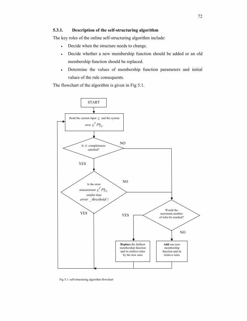
72
5.3.1. Description of the self-structuring algorithm
The key roles of the online self-structuring algorithm include:
• Decide when the structure needs to change.
• Decide whether a new membership function should be added or an old
membership function should be replaced.
• Determine the values of membership function parameters and initial
values of the rule consequents.
The flowchart of the algorithm is given in Fig 5.1.
NO
Read the current input z and the system
error C
TbPe
YES
START
Is ε -completeness
satisfied?
Is the error
measurement C
TbPe
smaller than
thresholderror _ ?
Replace the furthest
membership function
and its relative rules
by the new ones
Would the
maximum number
of rules be reached?
YES
NO
Add one new membership
function and its
relative rules
Fig 5.1: self-structuring algorithm flowchart
YES
NO

73
5.3.1.1. Criteria for rule generation
Two criteria for rule generation are system error and ε -completeness:
• System error:
C
TbPe represents the system error. In the adaptive law, the rule consequents are
adjusted to reduce C
TbPe . When 0=
C
TbPe , the output error is zero, and the rule
consequents do not need to change. Therefore, when C
TbPe is equal to or larger than
a predefined value thresholderror _ , a new membership function is considered.
• The ε -completeness:
In Gao [9], ε -completeness of fuzzy rules is defined as “for any input within the
operating range, there exists at least one fuzzy rule such that the match degree (or
firing strength) is not less than ε ”. To guarantee the ε -completeness, we make sure
that: for any input within the operating range, in every input dimension, there exists at
least one membership function such that the membership degree is not less than 0ε .
The relationship between ε and 0ε is n
0εε = , where n is the number of inputs. The
value of 0ε is usually selected as 5.00 =ε .
If one of the two criteria for rule generation is not satisfied, a new membership
function is considered. The algorithm then checks if ruleB would be exceeded if the
new membership function is added. If the answer is “no”, a new membership function
will be added. It the answer is “yes”, an old membership function will be replaced.
5.3.1.2. Adding a membership function and its related rules when the ε -
completeness is not satisfied
When the ε -completeness is not satisfied, and ruleB will not be reached, a new
membership function will be added.
Identify the input dimension to which the new membership function is added.
Since the ε -completeness is not satisfied, there is an input dimension that there is no
membership function with membership degree greater or equal to 0ε . The new
membership function is added to this input dimension.
Determine the parameters of the new membership function. Parameters of a
triangular membership function include its center, left point, and right point. When a
new membership function is added, its center is chosen as the current value of the
input variable. The left and right points are chosen as the centers of the left and right

74
neighbouring membership functions respectively. In cases when there is no left (or
right) neighbouring membership function, the left (or right) point is chosen such as
the distance to the center is equal to a predefined value (max_mf_distance). Thus,
max_mf_distance defines the maximum allowed distance between two neighbouring
membership functions.
To avoid membership functions being too close, a membership function is only
added when the distances between its center and the centers of the neighbouring
membership functions are greater than or equal to a predefined value
(min_mf_distance). Thus, min_mf_distance defines the minimum allowed distance
between two neighbouring membership functions.
To ensure that there are at most 2 membership functions activated at any time, the
neighbouring membership functions are also modified accordingly. The right point of
the left neighbouring membership function is modified to the center of new
( )txi
1mf 2mf 3mf
0
1
4mf
( )txi
1mf 2mf 3mf
0
1
0ε
a) Before a membership function is added
b) After a membership function is added
Figure 5.2: if ε -completeness is not satisfied and ruleB will not be reached

75
membership function. The left point of the right neighbouring membership function is
also modified to the center of the new membership function.
The new rules and the consequent values are determined as follows. All possible
rules made by the new membership function are generated. Since our proposed fuzzy
system is an unevenly-distributed grid-type, when a membership function is added,
12 −n new rules are made possible where n is the number of inputs. All the new rules’
consequents are, then initialized to the current output of the fuzzy system.
Fig 5.2 illustrates how a membership function is added in this case. Fig 5.2a
shows that the membership degree is less than 0ε . Thus, a membership function 4mf
is added at ( )txi as shown in fig 5.2b. It can be seen that the left point of 4mf is
chosen as the center of 3mf . Since there is no membership function on the right of
4mf , the right point of 4mf is chosen as ( )+txi max_mf_distance. The right point of
3mf is modified to the center of new membership function 4mf .
5.3.1.3. Replacing a membership function and its related rules when the ε -
completeness is not satisfied
When the ε -completeness is not satisfied, and ruleB will be reached, a
membership function will be replaced.
The new membership function and its related rules are determined the same way
in section 5.3.1.2.
The membership function to be removed is determined as follows. In the input
dimension to which the new membership function is added, the algorithm searches for
the furthest membership function from the current point. That furthest membership
function is the membership function to be removed. All rules related to the removed
membership function are also deleted from the rule base.
Fig 5.3 demonstrates how an old membership function is replaced in this case.
Fig 5.3a shows the membership functions before a membership function is replaced. It
can be seen that membership function 1mf is the furthest membership function from
( )txi . Thus, it will be replaced by a new one. Fig 5.3b shows the old membership
function 1mf (in fig 5.3a) is replaced by the new membership function 1mf . The
center of the new 1mf is chosen as ( )txi . The left point of 1mf is chosen as 3x . Since
there is no membership function on the right of new 1mf , the right point of 1mf is

76
chosen as ( )+txi max_mf_distance. Since there is no membership function on the
left of 2mf now, its left point is modified to ( )−txi max_mf_distance.
5.3.1.4. Adding a membership function and its related rules when C
TbPe is equal
to or larger than thresholderror _
When thresholderrorbPe C
T_≥ , and ruleB will not be reached, an old
membership function will be replaced.
Identify the input dimension to which the new membership function is added.
The following procedure is used. The rule with maximum firing strength at that
moment is selected. Then, the new membership function is added to the input with the
maximum membership function degree. The reason is that the large system error
( )txi
1mf 2mf 3mf
0
1
( )txi
1mf 2mf 3mf
0
1
4mf
1x 2x 3x
1x 2x 3x
a) Before a membership function is added
b) After a membership function is added
Figure 5.3: if thresholderrorbPeC
P_≥ , distance between ( )txi and the closest membership function
center ≥ hresholddistance_t , and ruleB will not be reached
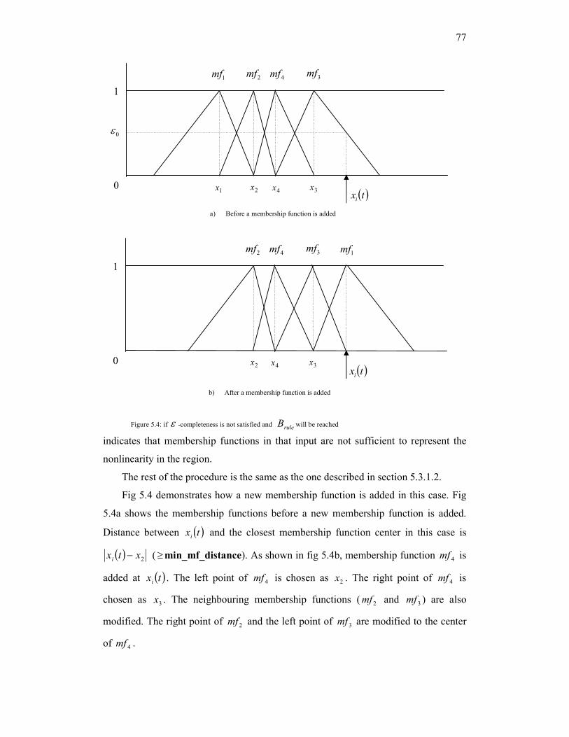
77
indicates that membership functions in that input are not sufficient to represent the
nonlinearity in the region.
The rest of the procedure is the same as the one described in section 5.3.1.2.
Fig 5.4 demonstrates how a new membership function is added in this case. Fig
5.4a shows the membership functions before a new membership function is added.
Distance between ( )txi and the closest membership function center in this case is
( ) 2xtxi − (≥min_mf_distance). As shown in fig 5.4b, membership function 4mf is
added at ( )txi . The left point of 4mf is chosen as 2x . The right point of 4mf is
chosen as 3x . The neighbouring membership functions ( 2mf and
3mf ) are also
modified. The right point of 2mf and the left point of 3mf are modified to the center
of 4mf .
( )txi
1mf 2mf 3mf
0
1
4mf
( )txi
1mf 2mf 3mf
0
1
4mf
0ε
1x 2x 3x 4x
2x 4x 3x
a) Before a membership function is added
b) After a membership function is added
Figure 5.4: if ε -completeness is not satisfied and ruleB will be reached

78
5.3.1.5. Replacing a membership function and its related rules when the error
measurement C
TbPe is equal to or larger than thresholderror _
When thresholderrorbPe C
T_≥ , and ruleB will be reached, a new membership
function will be added.
The new membership function and its related rules are determined the same way
in the section 5.3.1.4.
The old membership function to be replaced is determined the same way as in
section 5.3.1.3.
Fig 5.5 demonstrates how an old membership function is replaced in this case.
Fig 5.5a shows the functions before a membership function is replaced. Distance
between ( )txi and the closest membership function center is ( ) 3xtxi −
( )txi
1mf 2mf 3mf
0
1
4mf
( )txi
1mf 2mf 3mf
0
1
4mf
2x 1x 3x 4x
2x 3x 4x
a) Before a membership function is added
b) Before a membership function is added
Figure 5.5: if thresholderrorbPeC
P_≥ , distance between ( )txi and the closest membership
function center ≥ hresholddistance_t , and ruleB will be reached

79
(≥min_mf_distance). It can be seen that 1mf is the furthest membership function
from ( )txi . Thus, it will be replaced. Fig 5.5b shows the new membership function
1mf and the modified membership functions 3mf and 2mf . The center of 1mf is
chosen as ( )txi . The left point of 1mf is chosen as 3x . The right point of 1mf is
chosen as ( )+txi max_mf_distance. The right point of 3mf is modified to the center
of 1mf . The left point of 2mf is modified to ( )−txi max_mf_distance.
5.3.1.6. Parameters
The self-structuring algorithm has four design parameters. 0ε defines the
completeness of fuzzy rules, thresholderror _ defines the minimum level of error to
trigger structure change, min_mf_distance defines the minimum allowed distance
between two neighbouring membership functions, and max_mf_distance defines the
maximum allowed distance between two neighbouring membership functions.
Therefore, using larger values of 0ε or smaller values of thresholderror _ ,
min_mf_distance, or max_mf_distance will result in more rules being generated.
However, the number of rules is always bounded by ruleB .
5.3.2. SSDAFC
The stability of the SSDAFC is given in the following theorem.
Theorem 5.1 Given system ( )1.3 satisfying assumptions 4.1, 4.2, 4.3, and 5.1,
a controller ( )1.5 with the self-structuring algorithm described in section 5.3.1 and
the adaptive law
( ) ( )( )( )( )( )( )( )( )( )
0 and or
0 and if 0
0 and or
0 and or
if
≤=
≥=
>=
<=
<<
=
XbPeu
XbPeu
XbPeu
XbPeu
uuXbPe
jC
T
Lj
jC
T
Uj
jC
T
Lj
jC
T
Uj
UjLjC
T
j
ζγθ
ζγθζγθ
ζγθ
θζγ
θ&
will guarantee that:
iv. The adaptive parameters are bounded:
UjL uu ≤≤θ , Mj K1= .
v. The tracking error ( )te is bounded by:

80
( )( )
( )P
bPc
V
te
C
min
22
2
1,0max2
λ
εγα
+
≤
∗
, 0>∀t , ( )2.5
in which ( )( )( )PQ
max
min 1
λλ
α−
= , ( )0V and c are bounded positive constants.
vi. The system is Uniformly Ultimately Bounded (UUB), i.e. ( )te
converges to compact set eΩ in finite time:
( ) ( )( )
−≤=Ω
∗
1min
22
Q
bPtete
C
e λ
ε. ( )3.5
Proof
In theorem 4.1, we have proved the stability of fixed-structured systems. Here,
we also need to show the stability when the structure changes. If the Lyapunov
function is chosen as in ( )9.4 , it changes when the structure changes. Thus, it is rather
difficult to show the stability. To overcome this problem, we choose a new Lyapunov
function that also includes the not-yet-generated adaptive parameters:
( ) ( )∑∑+=
∗
=
∗ −+−+=N
Mk
kk
kM
j
jj
jTccePeV1
2
1
2
2
1
2
1
2
1θθ
γθθ
γ, ( )4.5
in which the values of not yet generated parameters kθ , NMk ,,1 K+= , are chosen
as their initialized values (these values are unknown and only required for analytical
purpose). Since P is positive definite and 0>jc , Mj K1= , 0>kc , NMk ,,1 K+= ,
it is obvious that 0≥V .
The stability analysis has two steps. First, we show the stability when the
structure is fixed. Then, we show that the system is stable at the time the structure
changes.
5.3.2.1. When the structure is fixed
From the adaptive law ( )8.4 , it is obvious that theorem5.1.i holds.
When the structure is fixed, M is unchanged. Using the fact that 0=∗jθ& ,
Mj K1= , and 0==∗ kk θθ && , NMk ,,1 K+= , the time derivative of V along the
trajectory of ( )6.4 is:

81
( ) ( ) ( )
1
2
1
11
+−+−−−= ∑∑
=
∗
=
∗ εζθθθθθγ
M
j
jjj
j
C
TM
j
jjj
jTXcbPeceQeV &&
( ) ( )( ) εθζγθθγ C
TM
j
jjC
T
jj
jTbPeXbPeceQeV +−−+−=⇔ ∑
=
∗
1
1
2
1 && .
This equation is exactly the same as ( )10.4 . Following the same procedure as in
theorem 4.1 (equations ( )10.4 to ( )15.4 ), we have theorem 5.1.ii and 5.1.iii hold.
5.3.2.2. When the structure changes
Now, to guarantee the stability of the system at all time, we need to show that the
system is stable when the structure changes.
This can be proved by showing that ( )tV defined in ( )4.5 does not change when
the structure changes. Let ct be the time that the structure changes and 1M , 2M be
the old and new numbers of rules respectively ( 21 MM < ). We will show that
( ) ( )+− = cc tVtV .
With the proposed self-structuring algorithm, the control signal is continuous at
ct :
( ) ( )+− = cc tutu . ( )5.5
Given system )1.3( , ( )5.5 leads to ( ) ( )+− = cc txtx and
( ) ( )+− = cc tete . )6.5(
From the adaptive law ( )8.4 , )6.5( leads to
( ) ( )+− = cjcj tt θθ , 11 Mj K= . )7.5(
Moreover, as we chose the values of inactivated adaptive parameters as the
values when they are activated, their values do not change at ct . Thus, we have:
( ) ( )+− = cjcj tt θθ , ( ) 21 ,,1 MMj K+= )8.5(
From )6.5( , )7.5( and )8.5( , we have:
( ) ( ) ( ) ( )( ) ( )( )
( ) ( ) ( )( ) ( )( )
( )++=
+∗
=
+∗++
+=
−∗
=
−∗−−−
=
−+−+=
−+−+=
∑∑
∑∑
c
N
Mk
ckk
kM
j
cjj
j
c
T
c
N
Mk
ckk
kM
j
cjj
j
c
T
c
tV
tctctePte
tctctePtetV
2
1
2
1
2
1
2
1
2
1
2
1
1
2
1
2
1
2
1
2
1
2
2
1
1
θθγ
θθγ
θθγ
θθγ

82
End of proof ◊
Remark 5.1 All remarks in chapter 4 are also valid for this SSDAFC scheme.
Remark 5.2 It should be noted that the structures generated by the self-
structuring algorithm are not the optimal ones. Our goal is not to find the optimal
solution, but to find a structure such that all variables are bounded (including the size
of the fuzzy controller) and the output follows the reference signal. The proposed self-
structuring algorithm satisfies this goal.
Remark 5.3 The main limitation of our approach is that it suffers from “the curse
of dimensionality”, the complexity increases exponentially with the number of inputs.
This is the trade-off for interpretability. Future research would be to develop a
SSDAFC scheme for high-order systems, in which simplicity is critical and
interpretability is less important.
5.4. Examples
5.4.1. Inverted pendulum
To demonstrate the proposed controller, its application to the inverted pendulum
given in section 3.4.1 is presented. The control objective is to make the angular
position 1xy = track the reference signal )sin(5.0)( ttr = .
The operating variable ranges are chosen as follows:
[ ]1,11 −∈x ; [ ]1,12 −∈x ; [ ]1,1−∈v .
The controller parameters are chosen as follows:
[ ]Tk 11= ;
=
100
020Q ;
=
1510
1025P ; 50=γ
10−=Lu ; 10=Uu .
To test the algorithm with different parameters, we perform simulations with 3
different setups as follows. As the fuzzy system has 3 premise variables,
thresholddistance _ and max_mf_distance are vectors with 3 elements. The
maximum allowed distance between 2 membership functions is chosen as half of the
input range, i.e max_mf_distance [ ]111= .
0ε thresholderror _ min_mf_distance max_mf_distance
ruleB
Setup1 0.5 0.5 [ ]2.02.02.0 [ ]111 100
Setup2 0.5 0.5 [ ]4.04.04.0 [ ]111 100

83
Setup3 0.5 0.5 [ ]4.04.04.0 [ ]111 20
The initial fuzzy system has only 1 rule (initialized to 0) with 1 membership
function in each input dimension as shown in fig 5.6.
The simulation results of setup 1 are shown in figures 5.7. A variable called self-
structuring flag is used to indicate when the self-structuring performs. When the self-
structuring flag switches from 1 to -1 or -1 to 1, it indicates a change of the fuzzy
system structure has occurred. It can be observed that the controller successfully
controls the inverted pendulum to track the sinusoidal signal )sin(5.0)( ttr = (Fig
5.7a). After 30s, the tracking error is as small as in the range [ ]01.0,01.0 +− (Fig 5.7b).
The control signal is always in the desired range [ ]10,10 +− (Fig 5.7c). Self-
structuring happens in the first 10s (Fig 5.7d). The final fuzzy system has 96 rules,
and the bound 100=ruleB is never exceeded. The final membership functions in each
input dimension are given in Figures 5.8.
The minimum allowed distance between two neighbouring membership functions
is defined by min_mf_distance. Thus, increasing min_mf_distance will result in
fewer rules. This is confirmed by simulation results of setup 2. After 30s, the tracking
error has reduced to within the range [ ]02.0,02.0 +− . The control signal is always in
the desired range [ ]10,10 +− . The final fuzzy system has 36 rules.
To test how the algorithm replaces membership functions and rules, we change
ruleB to 20 in setup 3. The results are shown in figures 5.9. It can be seen that the
tracking performance is very good. The tracking error is in the range [ ]02.0,02.0 +−
after 20s. The number of rules increases quickly in the first 5s to 18 rules. After that,
the number of rules never exceeds ruleB , i.e. 20 rules. It can be observed that the
algorithm replaces membership functions roughly at approximately 10, 14, 17, 32.5,
36, 45 and 54s. At those moments, there is no degradation in tracking performance.
This confirms that replacing membership functions does not affect the performance of
the control system. The membership functions of the fuzzy system at st 60= are
given in Figures 5.10.
The transient error shown in Fig 5.7c is better than the transient error shown in
Fig 5.9c. The reason is explained as follows. When a membership function (and its
corresponding rules) is added, the adaptive algorithm needs to make a large

84
adjustment due the initial error of the newly added adaptive parameters. As a result,
the control action changes relatively quick. Thus, the control performance temporarily
deteriorates. In Fig 5.9c, a higher number of rules is allowed. Thus, at the start of the
simulation, more membership functions are added due to large initial error. As a
consequence, performance in this case deteriorates more. When the structures of the
fuzzy systems are more stable (after 50s), the errors in both cases are similar.
5.4.2. Magnetic levitation
The magnetic levitation system is given in section 4.4.2. Now, we apply the
proposed DSAFC to control this system.
The variable ranges are:
[ ]5,01 ∈x ; [ ]10,52 −∈x ; [ ]10,10−∈v .
The controller parameters are:
[ ]Tk 11= ;
=
100
020Q ;
=
1510
1025P ; 50=γ .
25−=Lu ; 25=Uu (this implies that current i is in the range [ ]AA 5,5− ).
To test the algorithm with different parameters, we perform simulations with 3
different setups as follows:
0ε thresholderror _ min_mf_distance max_mf_distance
ruleB
Setup1 0.5 2 [ ]431 [ ]105.75.2 125
Setup2 0.5 0.5 [ ]431 [ ]105.75.2 125
Setup3 0.5 5 [ ]431 [ ]105.75.2 125
The initial fuzzy system has 8 rules (initialized to 0) with 2 membership functions
in each input dimension as shown in Figs 5.11.
The results of setup 1 are shown in Figures 5.12. It can be seen that the actual
output tracks the reference trajectory closely (Fig 5.12a), and thus, the controller
successfully controls the position of the magnet. The tracking error is never larger
than 0.3, and it quickly converges to near 0 after the set-point changes. The control
signal (Fig 5.12c) is always in the desired range [ ]AA 5,5− . The self-structuring
activity (Fig 5.12d) occurs in the first 20s of the simulation. Following this, the
number of rules remains unchanged at 48. The resulting fuzzy system has
membership functions for each input as shown in Figures 5.13.

85
The self–structuring algorithm suggests that increasing thresholderror _ will
result in fewer rules. This is confirmed by setups 2 and 3. Both applications produce
the desired performance. Setup 2 results in 64 rules. And setup 3 results in 36 rules
Both examples show that the desired performance can be achieved by different
sets of parameters of the self-structuring algorithm. Thus, the choice of parameters is
not critical. This gives designers the advantage of freely choosing parameters in
practice. This also demonstrates the ability of the self-structuring algorithm to
generate a satisfactory structure from different sets of parameters.
5.5. Conclusion
In this chapter, we have proposed a SSDAFC scheme for affine nonlinear
systems. The proposed control scheme has some advantages over some existing
SSDAFC schemes. It is relatively simpler and more computationally efficient. The
maximum number of rules of the fuzzy controller can be set explicitly and thus, never
exceed the hardware capacity. The stability is also proved when the structure changes.
The use of triangular membership functions increases the interpretability of the rules.
Application to an inverted pendulum system and a magnetic levitation system
demonstrate the effectiveness of the controller.
It should be noted that the structures generated by the self-structuring algorithms
are not the optimal ones. And the main limitation of our approach is that it suffers
from “the curse of dimensionality”.

86
-1 -0.8 -0.6 -0.4 -0.2 0 0.2 0.4 0.6 0.8 1
0
0.2
0.4
0.6
0.8
1
input1
Degre
e o
f m
em
bers
hip
mf1
Figure 5.6: initial membership functions for variables 1x ,
2x , and v
0 10 20 30 40 50 60
-0.6
-0.4
-0.2
0
0.2
0.4
0.6
Angula
r P
ositio
n(rad)
Time(second)
desired position
actual position
Figure 5.7a: position
0 10 20 30 40 50 60-0.25
-0.2
-0.15
-0.1
-0.05
0
0.05
0.1
0.15
Angula
r E
rror(ra
d)
Time(second) Figure 5.7b: error
0 10 20 30 40 50 60-15
-10
-5
0
5
10
15
Time(second)
Control S
ignal(N
)
Figure 5.7c: control signal
-1 -0.8 -0.6 -0.4 -0.2 0 0.2 0.4 0.6 0.8 1
0
0.2
0.4
0.6
0.8
1
input1
Degre
e o
f m
em
bers
hip
mf1 mf2mf3mf4
Figure 5.8a: final membership functions for variable 1x
-1 -0.8 -0.6 -0.4 -0.2 0 0.2 0.4 0.6 0.8 1
0
0.2
0.4
0.6
0.8
1
input2
Degre
e o
f m
em
bers
hip
mf1 mf2mf3mf4
Figure 5.8b: final membership functions for variable 2x
-1 -0.8 -0.6 -0.4 -0.2 0 0.2 0.4 0.6 0.8 1
0
0.2
0.4
0.6
0.8
1
input3
Degre
e o
f m
em
bers
hip
mf1mf2 mf3 mf4 mf5mf6
Figure 5.8c: final membership functions for variable v
0 10 20 30 40 50 600
50
100
Time(second)
Num
ber of ru
les
0 10 20 30 40 50 60
-1
0
1
Time(second)
Self-s
tructu
ring fla
g
Figure 5.7d: number of rules and self-structuring flag
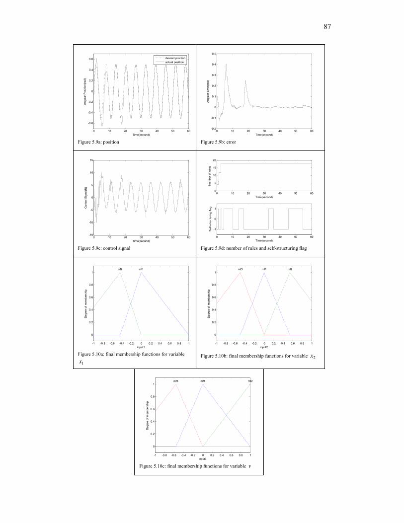
87
0 10 20 30 40 50 60-15
-10
-5
0
5
10
15
Time(second)
Control S
ignal(N
)
Figure 5.9c: control signal
0 10 20 30 40 50 600
5
10
15
20
Time(second)
Num
ber of ru
les
0 10 20 30 40 50 60
-1
0
1
Time(second)
Self-s
tructu
ring fla
g
Figure 5.9d: number of rules and self-structuring flag
-1 -0.8 -0.6 -0.4 -0.2 0 0.2 0.4 0.6 0.8 1
0
0.2
0.4
0.6
0.8
1
input1
Degre
e o
f m
em
bers
hip
mf1mf2
Figure 5.10a: final membership functions for variable
1x
-1 -0.8 -0.6 -0.4 -0.2 0 0.2 0.4 0.6 0.8 1
0
0.2
0.4
0.6
0.8
1
input2
Degre
e o
f m
em
bers
hip
mf1 mf2mf3
Figure 5.10b: final membership functions for variable 2x
0 10 20 30 40 50 60
-0.6
-0.4
-0.2
0
0.2
0.4
0.6
Angula
r P
ositio
n(rad)
Time(second)
desired position
actual position
Figure 5.9a: position
0 10 20 30 40 50 60-0.2
-0.1
0
0.1
0.2
0.3
0.4
0.5
Angula
r E
rror(ra
d)
Time(second) Figure 5.9b: error
-1 -0.8 -0.6 -0.4 -0.2 0 0.2 0.4 0.6 0.8 1
0
0.2
0.4
0.6
0.8
1
input3
Degre
e o
f m
em
bers
hip
mf1 mf2mf3
Figure 5.10c: final membership functions for variable v

88
0 0.5 1 1.5 2 2.5 3 3.5 4 4.5 5
0
0.2
0.4
0.6
0.8
1
input1
Degre
e o
f m
em
bers
hip
mf1 mf2
Fig 5.11a: initial membership functions for variable 1x
-5 0 5 10
0
0.2
0.4
0.6
0.8
1
input2
Degre
e o
f m
em
bers
hip
mf1 mf2
Fig 11b: initial membership functions for variable 2x
-10 -8 -6 -4 -2 0 2 4 6 8 10
0
0.2
0.4
0.6
0.8
1
input3
Degre
e o
f m
em
bers
hip
mf1 mf2
Fig 11c: initial membership functions for variable v
0 10 20 30 40 50 60 70 80 900
0.5
1
1.5
2
2.5
3
3.5
Outp
ut(cm
)
Time(second)
reference trajactory
actual output
desired output
Figure 5.12a: position of the magnet
0 10 20 30 40 50 60 70 80 90-0.5
-0.4
-0.3
-0.2
-0.1
0
0.1
0.2
Figure 5.12b: position error
0 10 20 30 40 50 60 70 80 90-2
-1
0
1
2
3
4
Current(am
p)
Time(second)
Figure 5.12c: control signal (amp)
0 10 20 30 40 50 60 70 80 900
20
40
60
Num
ber of ru
les
Time(second)
0 10 20 30 40 50 60 70 80 90-1
-0.5
0
0.5
1
Time(second)
Self-s
tructu
ring fla
g
Figure 5.12d: number of rules

89
0 0.5 1 1.5 2 2.5 3 3.5 4 4.5 5
0
0.2
0.4
0.6
0.8
1
input1
Degre
e o
f m
em
bers
hip
mf1 mf2mf3 mf4
Fig 5.13a: final membership functions for variable 1x
-5 0 5 10
0
0.2
0.4
0.6
0.8
1
input2
Degre
e o
f m
em
bers
hip
mf1 mf2mf3 mf4
Fig 5.13b: final membership functions for variable 2x
-10 -8 -6 -4 -2 0 2 4 6 8 10
0
0.2
0.4
0.6
0.8
1
input3
Degre
e o
f m
em
bers
hip
mf1 mf2mf3
Fig 5.13c: final membership functions for variable v

90
6. Chapter 6
SELF-STRUCTURING DIRECT ADAPTIVE FUZZY CONTROL
FOR NON-AFFINE NONLINEAR SYSTEMS3
6.1. Introduction
In chapter 3, 4 and 5, we have discussed AFC of affine nonlinear systems.
However, there are many practical nonlinear systems, e.g. chemical reactions and PH
neutralization, whose inputs may not be expressed in affine forms. Adaptive
intelligent control for non-affine nonlinear systems is more difficult and challenging.
Consider SISO non-affine nonlinear systems described as follows:
1
32
21
),(
xy
uxfx
xx
xx
n
=
=
=
=
&
K
K
&
&
( )1.6
where Ru∈ is the control input, Ry∈ is the output, ),( uxf is an unknown nonlinear
continuous function, T
nxxxx ),,,( 2,1 K= is the state vector of the system, which is
assumed available for measurement. In this chapter, we will investigate SSDAFC of
nonlinear systems in the form ( )1.6 .
A short survey about the topic is given in section 6.2. Then, the SSDAFC for
nonaffine nonlinear systems ( )1.6 is given in section 6.3. It is followed by application
to two nonaffine nonlinear systems. Finally, conclusion is given in section 6.5
6.2. Literature review
Because the control input does not appear linearly, the well-known feedback
linearization technique is not applicable to non-affine nonlinear systems. An explicit
expression for the ideal control cannot be obtained. Thus, more complex
mathematical tools are needed. In [33], the Taylor series expansion method is used to
transform the original system into an affine-like one. In [34], the mean value theorem
3 The content of this chapter has been published in Fuzzy Sets and Systems:
P.A. Phan, and T.J. Gale, “Direct Adaptive Fuzzy Control with a Self-Structuring Algorithm”, Fuzzy Sets and Systems, in press.

91
and Nussbaum-Gain functions are used. [2, 35] employ the implicit function theorem
and the mean value theorem to show the existence of ideal feedback control. [36-38]
propose a pseudo-control scheme and require the contraction condition to show that
the pseudo-error can be cancelled by an output of an adaptive neural network (or an
adaptive fuzzy system).
Also, more requirements are required. Besides the controllability condition
( )0
,>
∂
∂
u
ux, [33] requires the determination of a lower bound Lg such that
( )0
,>≥
∂
∂Lg
u
uxf. [36-38] require the determination of a design parameter c such
that ( )
∂
∂>
u
uxfc
,
2
1. [2, 35] require that the derivative of
( )u
uxf
∂
∂ , is bounded and
that a design parameter vk is chosen such as 0kkv > , where 0k is an unknown
positive constant.
To our knowledge, Park et all [37] is the only online self-structuring AFC
available for non-affine nonlinear systems. As discussed in chapter 5, the draw backs
of Park’s self-structuring algorithm are the even distribution of membership functions
and the unrestricted growth of the number of rules. Moreover, in the design of the
controller, it is required to select a design parameter c such that ( )
∂
∂>
u
uxfc
,
2
1.
Thus, knowledge of the upper bound of ( )u
uxf
∂
∂ , is needed, or a rather conservative
value of c must be chosen. Thus, it is desirable to develop a more efficient AFC
scheme for non-affine nonlinear systems.
In this chapter, we propose a new SSDAFC for non-affine nonlinear systems.
First, the existence of an implicit ideal control law is shown using the implicit
function theorem. Then, using an extension of the universal property, we transform
the error dynamic to the same one as for affine nonlinear systems. Thus, theorem 5.1
can be applied. The main contributions are:
• Propose a DAFC scheme for non-affine nonlinear with less restrictions on
( )u
uxf
∂
∂ ,. The only requirement of the control plant is the controllability
condition ( )
0,
>∂
∂
u
ux. And there is no restriction on the design parameters.

92
• Propose using the self-structuring algorithm described in chapter 5 for
DAFC of non-affine nonlinear systems.
6.3. SSDAFC for non-affine nonlinear systems
Control objective is to design an adaptive fuzzy controller for non-affine
systems described by ( )1.6 such that:
The closed-loop system must be stable in the sense that all the variables in the
closed-loop system must be bounded.
The output )(ty of the system follows a continuous reference signal nCtr ⊂)( .
Assumption 6.1: controllability condition
( )0
,>
∂
∂
u
uxf
hold for all ( ) Rux x ×Ω∈, with a controllability region xΩ .
Assumption 6.2: Define Tnrrrrr ],,,[ )1( −= K&&&&&& . We assume that 0rr ≤ and
1
)( rr n ≤ with known constants 0, 10 >rr .
Assumption 6.3 We can determine the upper bound ruleB of the required number
of rules that achieves the desired approximation accuracy.
6.3.1. Existence of an ideal control law
Let yre −= , ( )( )Tneeeee 1,,,, −= K&&& , and ( )Tnkkkk ,,, 21 K= be such that the
polynomial 1
1 ksks n
n
n +++ −K is Hurwitz stable. The ideal control law is chosen to
obtain ( ) ( )1
21
−−−−=−= n
n
Tn ekekekeke K& , yre −= , which implies that 0lim =+∞→e
t.
Let ( ) ekrvTn += . ( )2.6
Adding and subtracting v to ( )1.6 gives
( ) ( ) vduxfekeTn +−−−= , ( )3.6
Now, we prove that there exists an ideal control signal ( )vxu ,∗ such that
( )( ) vvxuxf =∗ ,, for ( ) RRvx n ×∈, .
Reintroduce lemma 2.8 that is given in [2]:
Lemma 6.1. Assume that RRRf n →×: is continuously differentiable and
there exists a positive constant q such that ( ) 0, >>∂∂
quxfu
for all

93
( ) RRux n ×∈, . Then there exists a unique continuous smooth function RRg n →:
such that ( )( ) 0, =xgxf .
Proof is given in [2]◊
Let ( ) 1, +∈= nRvxX and ( ) ( ) vuxfuXF −= ,, . We have
( ) ( )0
,,>
∂∂
−∂
∂=
∂∂
u
v
u
uxf
u
uXF as 0=
∂∂u
v and
( )0
,>
∂
∂
u
uxf (assumption 1). Thus, we
can apply lemma 1 for ( )uXF , . Applying lemma 1, there exists a unique continuous
smooth function ( )Xu ∗ such that ( )( ) 0, =∗ XuXF , i.e.
( )( ) vXuxf =∗, . ( )4.6
6.3.2. Stability analysis
From ( )3.6 and ( )4.6 , we have
( ) ( )( ) ( )( )[ ]XuxfXuxfekeTn ,, −+−= ∗ ( )5.6
Similar to chapter 5, we let ( ) ( )TN
TT
in
T
ac θθθθθθ K,, 21== be the adaptive
parameter vector of the final fuzzy controller, in which ( )TMac θθθθ K,, 21= ,
( NM ≤ ) is the vector of adaptive parameters already activated, and
( )TNMMin θθθθ K,, 21 ++= is the vector of adaptive parameters not yet generated
(inactivated). We will employ a fuzzy system in the form ( )2.2 to approximate ( )Xu∗ :
( ) ( ) ( )∑=
==M
j
jjac XXuXu1
ˆ ζθθ . ( )6.6
In the literature, the universal approximation property is used to show that there
exists a fuzzy controller in the form ( )6.6 to approximate an ideal control signal with
arbitrary accuracy. Here, an extended version of that is introduced:
Lemma 6.2. Given an arbitrary 0>∗ε , there exist
( ) ( ) ( ) ( )( )TM XXXX ζζζζ K,, 21= and an ideal parameter vector ( )TMθθθθ K,, 21=∗ such
that
( )( ) ( )( ) ( ) ( ) εζθθ +−=− ∑=
∗∗M
j
jjj
j XcXuxfXuxf1
,, ( )7.6
where ∗≤ εε and jc are some positive constants.
The proof is given in appendix 6.A◊
Substituting ( )7.6 to ( )5.6 gives the error dynamics:

94
( ) ( ) ( ) εζθθ +−+−= ∑=
∗M
j
jjj
jTn Xceke1
. ( )8.6
In the vector form,
( ) ( )
+−+Λ= ∑
=
∗ εζθθM
j
jjj
j
CC Xcbee1
& ( )9.6
where
n321
C
k-k-k-k-
1000
0100
0010
=Λ
L
L
MOMMM
L
L
,
=
1
0
0
0
MCb .
Since CΛ is a stable matrix, there exists a unique positive definite symmetric
nn × matrix P which satisfies the Lyapunov equation:
QPP C
T
C −=Λ+Λ )10.6(
where Q is an arbitrary nn × positive definite matrix chosen such that ( ) 1min >Qλ .
Assumption 6.4 We can determine the upper and lower bounds of the ideal
control signal:
( ) UL uXuu ≤≤ ∗ , XX Ω∈∀ .
As the error dynamic ( ).6 is the same as equation ( )6.4 , the controllers proposed
in chapter 4,5 can be applied to system ( )1.6 . The control scheme is stated in the
following theorem
Theorem 6.1 Given system ( )1.6 satisfying assumptions 6.1, 6.2, 6.3, and 6.4,
a controller
( ) ( )∑=
==M
j
jjac XXuu1
ˆ ζθθ
with the self-structuring algorithm described in section 5.1.1 and the adaptive law
( ) ( )( )( )( )( )( )( )( )( )
0 and or
0 and if 0
0 and or
0 and or
if
≤=
≥=
>=
<=
<<
=
XbPeu
XbPeu
XbPeu
XbPeu
uuXbPe
jC
T
Lj
jC
T
Uj
jC
T
Lj
jC
T
Uj
UjLjC
T
j
ζγθ
ζγθζγθ
ζγθ
θζγ
θ&
will guarantee that:

95
vii. The adaptive parameters are bounded:
UjL uu ≤≤θ , Mj K1= .
viii. The tracking error ( )te is bounded by:
( )( )
( )P
bPc
V
te
C
min
22
2
1,0max2
λ
εγα
+
≤
∗
, 0>∀t ,
in which ( )( )( )PQ
max
min 1
λλ
α−
= , ( )0V is a bounded positive constant, and c is a positive
constant that can be made arbitrarily small by tuning the adaptive parameter γ .
ix. The system is Uniformly Ultimately Bounded (UUB), i.e. ( )te
converges to compact set eΩ in finite time:
( ) ( )( )
−≤=Ω
∗
1min
22
Q
bPtete
C
e λ
ε.
Proof
As the error dynamic ( )9.6 is the same as equation ( )6.4 , the proof is the same as
in theorem 5.1.
End of poof◊
As the result is the same as in chapter 4 and 5, remarks given in chapters 4 and 5
apply.
6.4. Examples
6.4.1. Application 1
To demonstrate the design procedure and performance, we apply our controller to
control a nonaffine nonlinear system that are presented in [2, 35-37]. The dynamic
equations of the system are:
( ) ( )1
2
2
32
12
21
1.0sin11.015.0
xy
uuxuxx
xx
=
++++=
=
&
&
.
We suppose that there is no prior knowledge of the system except that
( )0
,>
∂∂
u
uxF, which can be easily checked. The initial state is ( ) [ ]Tx 0 00 = . The

96
control objective is to make the output ( )ty follow a desired reference
( ) ( ) ( )tttr 5.0cossin += .
The operating input ranges are chosen as follows:
[ ]5,51 −∈x ; [ ]5,52 −∈x ; [ ]5,5−∈v .
The controller’s parameters are specified as follows:
[ ]Tk 11= ,
=
100
020Q ,
=
1510
1025P , 100=γ , 05.0=σ .
The structure-learning parameters are as follows:
5.00 =ε , 5_ =thresholderror , min_mf_distance [ ]111= ,
max_mf_distance [ ]555= , 30=rulesB .
The initial fuzzy system has only 1 rule (initialized to 0) with 1 membership
function in each input dimension as shown in Fig 6.1.
The simulation results are shown in Fig 6.2. It can be observed that the controller
successfully controls the nonaffine nonlinear system to track the reference signal
( ) ( )tttr 5.0cossin)( += (Fig 6.2a). After 10s, the tracking error is within the range
[ ]02.0,02.0 +− (Fig 6.2b). The control signal is bounded (Fig 6.2c). The chattering
phenomena can be reduced by reducing the adaptive gain γ , but at the expense of
increasing the tracking error. Self-structuring happens in the first 5s (Fig 6.2d). A
variable called self-structuring flag is used to indicate when the self-structuring
performs. When the self-structuring flag switches from 1 to -1 or -1 to 1, it indicates a
change of the fuzzy system structure has occurred. The final fuzzy system has 12
rules, and the rulesB is never reached. The final membership functions in each input
dimension are given in Fig 6.3.
To test how the algorithm replaces membership functions and rules, we change
the thresholderror _ from 5 to 4, thus more rules are generated. The results are
shown in Fig 6.4. The number of rules increases in the first 15s to 24 rules (Fig 6.4d).
After that, the number of rules never exceeds rulesB . It can be observed that the
algorithm replaces membership functions at approximately 19s and 28s. At those
moments, there is no degradation in tracking performance (Fig 6.4a). This confirms
that replacing membership functions does not effect the performance of the control
system. The membership functions of the fuzzy system at st 30= is given in Fig 6.5.
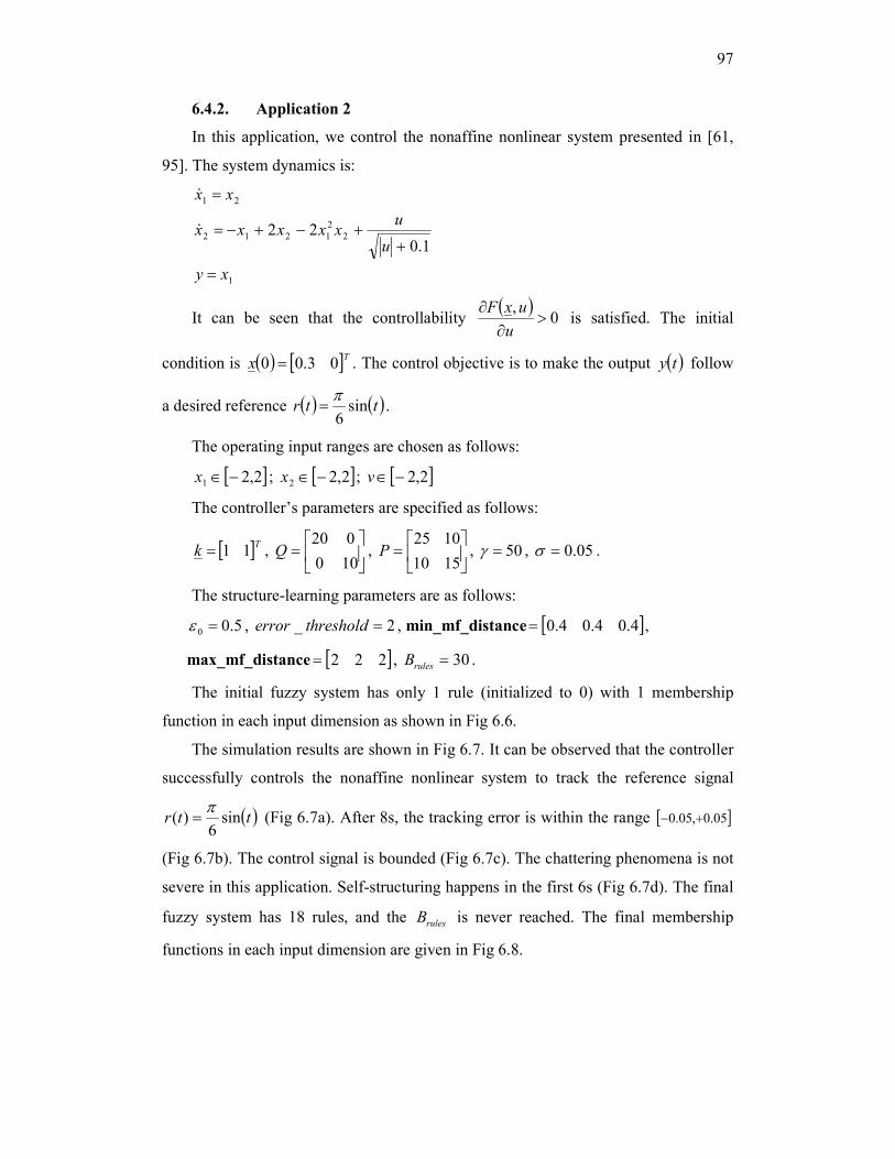
97
6.4.2. Application 2
In this application, we control the nonaffine nonlinear system presented in [61,
95]. The system dynamics is:
1
2
2
1212
21
1.022
xy
u
uxxxxx
xx
=
++−+−=
=
&
&
It can be seen that the controllability ( )
0,
>∂
∂
u
uxF is satisfied. The initial
condition is ( ) [ ]Tx 03.00 = . The control objective is to make the output ( )ty follow
a desired reference ( ) ( )ttr sin6
π= .
The operating input ranges are chosen as follows:
[ ]2,21 −∈x ; [ ]2,22 −∈x ; [ ]2,2−∈v
The controller’s parameters are specified as follows:
[ ]Tk 11= ,
=
100
020Q ,
=
1510
1025P , 50=γ , 05.0=σ .
The structure-learning parameters are as follows:
5.00 =ε , 2_ =thresholderror , min_mf_distance [ ]4.04.04.0= ,
max_mf_distance [ ]222= , 30=rulesB .
The initial fuzzy system has only 1 rule (initialized to 0) with 1 membership
function in each input dimension as shown in Fig 6.6.
The simulation results are shown in Fig 6.7. It can be observed that the controller
successfully controls the nonaffine nonlinear system to track the reference signal
( )ttr sin6
)(π
= (Fig 6.7a). After 8s, the tracking error is within the range [ ]05.0,05.0 +−
(Fig 6.7b). The control signal is bounded (Fig 6.7c). The chattering phenomena is not
severe in this application. Self-structuring happens in the first 6s (Fig 6.7d). The final
fuzzy system has 18 rules, and the rulesB is never reached. The final membership
functions in each input dimension are given in Fig 6.8.

98
6.5. Conclusion
In this chapter, we have extended the SSDAFC proposed in chapter 5 to a class of
nonaffine nonlinear systems ( )1.6 :
1
32
21
),(
xy
uxfx
xx
xx
n
=
=
=
=
&
K
K
&
&
All features of the self-structuring algorithm are still valid. Moreover, the control
scheme requires less restriction than some existing AFC schemes for nonaffine
nonlinear systems. Application to two nonaffine nonlinear systems is shown to
demonstrate the approach.
In next chapter, the SSDAFC scheme is further extended to a large class of
nonaffine nonlinear systems and a class of nonlinear systems in triangular forms.

99
-5 -4 -3 -2 -1 0 1 2 3 4 5
0
0.2
0.4
0.6
0.8
1
input1
Degre
e o
f m
em
bers
hip
mf1
Fig 6.1: initial membership functions of variables 1x , 2x ,
and v
0 2 4 6 8 10 12 14 16 18 20-2
-1.5
-1
-0.5
0
0.5
1
1.5
2
outp
ut and d
esired o
utp
ut
Time(second)
desired output
actual output
Fig 6.2a: Desired output and actual output
0 2 4 6 8 10 12 14 16 18 20-0.2
0
0.2
0.4
0.6
0.8
1
trackin
g e
rror
Time(second)
Fig 6.2b: Tracking error
0 2 4 6 8 10 12 14 16 18 20-20
-15
-10
-5
0
5
10
15
20
25
control sig
nal
Time(second)
Fig 6.2c: Control signal
0 2 4 6 8 10 12 14 16 18 200
5
10
15
Time(second)
Num
ber of ru
les
0 2 4 6 8 10 12 14 16 18 20
-1
0
1
Time(second)
Self-s
tructu
ring fla
g
Fig 6.2d: Number of rules and self-structuring flag

100
-5 -4 -3 -2 -1 0 1 2 3 4 5
0
0.2
0.4
0.6
0.8
1
input1
Degre
e o
f m
em
bers
hip
mf1 mf2
Fig 6.3a: final membership functions of variable 1x
-5 -4 -3 -2 -1 0 1 2 3 4 5
0
0.2
0.4
0.6
0.8
1
input2
Degre
e o
f m
em
bers
hip
mf1mf2
Fig 6.3b: final membership functions of variable 2x
-5 -4 -3 -2 -1 0 1 2 3 4 5
0
0.2
0.4
0.6
0.8
1
input3
Degre
e o
f m
em
bers
hip
mf1mf2 mf3
Fig 6.3c: final membership functions of variable v

101
0 5 10 15 20 25 30-2
-1.5
-1
-0.5
0
0.5
1
1.5
2
outp
ut and d
esired o
utp
ut
Time(second)
desired output
actual output
Fig 6.4a: Desired output and actual output for the case
4_ =thresholderror
0 5 10 15 20 25 30-0.4
-0.2
0
0.2
0.4
0.6
0.8
1
1.2
trackin
g e
rror
Time(second)
Fig 6.4b: Tracking error for the case
4_ =thresholderror
0 5 10 15 20 25 30
-25
-20
-15
-10
-5
0
5
10
15
20
25
control sig
nal
Time(second)
Fig 6.4c: Control signal for the case
4_ =thresholderror
0 5 10 15 20 25 300
10
20
30
Time(second)
Num
ber of ru
les
0 5 10 15 20 25 30
-1
0
1
Time(second)
Self-s
tructu
ring fla
g
Fig 6.4d: Number of rules and self-structuring flag for the
case 4_ =thresholderror

102
-5 -4 -3 -2 -1 0 1 2 3 4 5
0
0.2
0.4
0.6
0.8
1
input1
Degre
e o
f m
em
bers
hip
mf1mf2 mf3
Fig 6.5a: final membership functions of variable 1x for the
case 4_ =thresholderror
-5 -4 -3 -2 -1 0 1 2 3 4 5
0
0.2
0.4
0.6
0.8
1
input2
Degre
e o
f m
em
bers
hip
mf1 mf2
Fig 6.5b: final membership functions of variable 2x for
the case 4_ =thresholderror
-5 -4 -3 -2 -1 0 1 2 3 4 5
0
0.2
0.4
0.6
0.8
1
input3
Degre
e o
f m
em
bers
hip
mf1mf2 mf3 mf4
Fig 6.5c: final membership functions of variable v for the
case 4_ =thresholderror

103
-2 -1.5 -1 -0.5 0 0.5 1 1.5 2
0
0.2
0.4
0.6
0.8
1
input1
Degre
e o
f m
em
bers
hip
mf1
Fig 6.6: initial membership functions of variables 1x , 2x ,
and v
0 2 4 6 8 10 12 14 16 18 20-1
-0.8
-0.6
-0.4
-0.2
0
0.2
0.4
0.6
0.8
1
outp
ut and d
esired o
utp
ut
Time(second)
desired output
actual output
Fig 6.7a: Desired output and actual output
0 2 4 6 8 10 12 14 16 18 20
-0.25
-0.2
-0.15
-0.1
-0.05
0
0.05
0.1
0.15
0.2
0.25
trackin
g e
rror
Time(second)
Fig 6.7b: Tracking error
0 2 4 6 8 10 12 14 16 18 20-30
-20
-10
0
10
20
30
control sig
nal
Time(second)
Fig 6.7c: Control signal
0 2 4 6 8 10 12 14 16 18 200
5
10
15
20
Time(second)
Num
ber of ru
les
0 2 4 6 8 10 12 14 16 18 20
-1
0
1
Time(second)
Self-s
tructu
ring fla
g
Fig 6.7d: Number of rules and self-structuring flag

104
-2 -1.5 -1 -0.5 0 0.5 1 1.5 2
0
0.2
0.4
0.6
0.8
1
input1
Degre
e o
f m
em
bers
hip
mf1 mf2mf3
Fig 6.8a: final membership functions of variable 1x
-2 -1.5 -1 -0.5 0 0.5 1 1.5 2
0
0.2
0.4
0.6
0.8
1
input2
Degre
e o
f m
em
bers
hip
mf1 mf2
Fig 6.8b: final membership functions of variable 2x
-2 -1.5 -1 -0.5 0 0.5 1 1.5 2
0
0.2
0.4
0.6
0.8
1
input3
Degre
e o
f m
em
bers
hip
mf1 mf2mf3
Fig 6.8c: final membership functions of variable v

105
7. Chapter 7
EXTENSION TO THE CONTROL OF OTHER CLASSES OF SISO
NON-AFFINE NONLINEAR SYSTEMS
7.1. Introduction
In the last chapter, we have investigated SSDAFC for non-affine systems in the
normal form:
1
32
21
),(
xy
uxfx
xx
xx
n
=
=
=
=
&
K
K
&
&
( )1.7
where Ru∈ is the control input, Ry∈ is the output, ),( uxf is an unknown
nonlinear continuous function, T
nxxxx ),,,( 2,1 K= is the state vector of the system,
which is assumed available for measurement. In this chapter, we will extend the
results to two broader classes of systems.
In particular, in section 7.2, we will extend SSDAFC to SISO non-affine
nonlinear systems in the general form [2, 3, 44, 63, 65, 66]
( )xhy
uxfx
=
= ),( )2.7(
where Ru∈ is the control input, Ry∈ is the output, T
nxxxx ),,,( 2,1 K= is the state
vector of the system, ( ) ( ) ( ) ( )( )Tn uxfuxfuxfuxf ,,,,,,, 21 K= is a vector of unknown
nonlinear continuous functions, and ( )xh is an unknown continuous function.
Then, in section 7.3, we will consider the control of systems in triangular form [2,
34, 56]:
( )( )
1
1
111
,,,
1,,1,,
xy
uxxfx
nixxfx
nnn
ii
=
=
−== +
K&
KK&
)3.7(
where Ru∈ is the control input, Ry∈ is the output, T
nxxxx ),,,( 2,1 K= is the state
vector of the system, ( )•if , ni K1= are unknown continuous functions.

106
As we will show later, the control of systems )2.7( and )3.7( requires knowledge
of the output y and its derivatives ( )iy , ki K1= , nk ≤ . In practice, the derivatives
of y are sometimes not available for measurement. Output feedback control, in which
only the output is required, is an approach to overcome this difficulty. In section 7.4,
we will use a high-gain observer to observe the derivatives of y and thus propose an
output feedback SSDAFC scheme.
7.2. SSDAFC of systems in the form )2.7(
Fixed-structured adaptive intelligent control has been proposed for system )2.7(
in the literature [2, 3, 44, 63, 65, 66]. The key idea is to show that system )2.7( can be
transformed to the form ( )1.7 if certain conditions are satisfied. Then, adaptive
intelligent control for system ( )1.7 can be applied to system )2.7( .
However, to our knowledge, no self-structuring adaptive intelligent control
approach for system )2.7( has been in the literature. Therefore, inspired by the
previous works, we first show that system )2.7( can be transformed to the form ( )1.7 .
Then, our SSDAFC proposed in chapter 6 can be applied to system )2.7( .
Definition 7.1 Lie derivative
Let hL f denote the Lie derivative of the function ( )xh with respect to the vector
field ( )uxf , :
( )[ ] ( )uxfx
xhhL f ,
∂∂
=
Higher-order derivatives are defined recursively as ( )hLLhL k
ff
k
f
1−= , 1>k .
Definition 7.2 Strong relative degree
For n
x Rx ⊂Ω∈ and Ru u ⊂Ω∈ , system )2.7( is said to have a strong relative
degree ρ in ux Ω×Ω if there exists a positive integer ∞≤≤ ρ1 such that
[ ]0=
∂
∂
u
hLi
f, 1,,1,0 −= ρKi ,
[ ]0≠
∂
∂
u
hL f
ρ
for all ( ) uxux Ω×Ω∈, .
To continue, we consider two cases: system )2.7( with strong relative degree
n=ρ , and system )2.7( with strong relative degree n<ρ .

107
7.2.1. Control of system )2.7( with strong relative degree n=ρ
With n=ρ , system )2.7( can be transformed into a normal form )1.7( [2]
( )
=
=
−== +
1
1
,
1,,1,
ξ
ξξ
ξξ
y
ub
ni
n
ii
&
K&
)4.7(
where ( ) nixhLi
fi ,,1,1K== −ξ , ( ) ( )xhLub n
f=,ξ , and [ ] ξξξξξ Ω∈= T
nK21 ,
xx Ω∈=Ω ξξ .
From definition 7.2, ( )
0,
≠∂
∂
u
ub ξ uu Ω∈Ω∈∀ ,ξξ , i.e. assumption 6.1 is
satisfied. Thus, given system )2.7( with strong relative degree n=ρ , the self-
structuring DAFC proposed in 6.3 applied to system )4.7( guarantees that all signal
of system )2.7( are bounded and the tracking error is uniformly ultimately bounded
(UUB).
Remark 7.1 After the transformation, the output and its derivatives
( )( ) ( )Tn
Tnyyy 121
1 ,,,,,, −− = ξξξ KK& are needed to construct the controller. If these
signals are not available, they need to be estimated. In section 7.4, we will present an
output feedback SSDAFC scheme, in which only the output is measurable. Its
derivatives will be estimated using observers.
7.2.2. Control of system )2.7( with strong relative degree n<ρ
With n<ρ , after the transformation, we have the system in the normal
form:
( )( )
=
=
=
−== +
1
1
,,
,,
1,,1,
ξ
ηξη
ηξξ
ρξξ
ρ
y
uq
ub
iii
&
&
K&
)5.7(
where ( ) ρξ ,,1,1K== − ixhLi
fi , ( ) ( )xhLub n
f=,ξ , ( ) ( ) ρηξ ρ −== + nixhLuq i
fi ,,1,,, K ,
( ) ηξηξ Ω×Ω∈, , xx Ω∈=Ω×Ω ηξηξ , .
If applying the SSDAFC scheme in section 6.3 to the ξ -subsystem

108
( )
=
=
−== +
1
1
,,
1,,1,
ξ
ηξξ
ρξξ
ρ
y
ub
iii
&
K&
, )6.7(
the states η is completely unobservable. Thus, η is not guaranteed to be bounded.
The dynamics ( )uq ,,ηξη =& is called the internal dynamics. And with 0=ξ ,
( )uq ,,0 ηη =& is addressed as the zero dynamics.
To assure the boundedness of the internal dynamics, the following assumption is
required [63, 65, 66]:
Assumption 7.1 The system )2.7( is hyperbolically minimum-phase, i.e. the zero
dynamics is exponentially stable.
In [63, 65, 66], the authors show that assumption 7.1 implies that bounded ξ
leads to bounded η .
Therefore, given system ( )2.7 with zero dynamics, i.e. with strong relative
degree n<ρ , if assumption 7.1 is satisfied, the self-structuring DAFC scheme
proposed in section 6.2 applied to the ξ -subsystem )6.7( guarantees all signals of
)2.7( are bounded and the tracking error is UUB.
7.3. SSDAFC of systems in the triangular form )3.7(
The class of systems in the triangular form is a very popular class of SISO
nonlinear systems. This class includes both strict-feedback systems and pure-feedback
systems. A brief review of adaptive intelligent control of systems in the triangular
form )3.7( has been given in chapter 2. Adaptive back-stepping is the main technique.
Using the adaptive back-stepping technique, we can construct a backstepping-based
SSDAFC for system )3.7( , in which an adaptive fuzzy system equipped with the self-
structuring algorithm proposed in chapter 5 is used at every step to approximate the
virtual control at every step. However, a serious draw back of the backstepping
technique is that it needs at least one adaptive intelligent system at every step. This
dramatically increases the complexity of the controller as the order of the system
increases.
Therefore, here, we propose a SSDAFC for system )3.7( , in which only one
adaptive fuzzy system is required no matter what the order of the system is. The idea

109
is to show that we can transform system )3.7( to the form )1.7( . Then, the SSDAFC
proposed in chapter 6 can applied to system )3.7( .
First, we need to state the controllability condition for system )3.7( as commonly
made in the literature:
Assumption 7.2 System )3.7( satisfies:
( )0
,,
1
11 ≠∂
+
+
i
ii
x
xxf K, 1,,1 −= ni K and
( )0
,,,1 ≠∂
∂
u
uxxf nn K n
x Rx ⊂Ω∈∀ . )7.7(
Now, we need to show that if assumption 7.2 is satisfied then system )3.7( has
strong relative degree n=ρ :
• The first Lie derivative of the output y of system )3.7( is:
( )[ ] ( ) ( ) ( )211211
1
1 ,,, xxfxxfx
xuxf
x
xyyL f =
∂
∂=
∂∂
= .
Obviously, [ ]
0=∂
∂
u
yL f n
x Rx ⊂Ω∈∀ .
• The second Lie derivative of the output y of system )3.7( is:
[ ] ( ) ( ) ( ) ( ) ( )3212
2
211211
1
2112 ,,,
,,
, xxxfx
xxfxxf
x
xxfuxf
x
yLyL
f
f ∂∂
+∂
∂=
∂
∂= .
From assumption 7.2, ( )
0,
2
211≠
∂
∂
x
xxf and
( )0
,,
3
3212 ≠∂
∂
x
xxxf n
x Rx ⊂Ω∈∀ ,
the right-hand side is guaranteed to depend on 3x . Thus, we can let
( ) ( ) ( ) ( ) ( )32123212
2
211
211
1
211 ,,,,,
,,
xxxFxxxfx
xxfxxf
x
xxf=
∂
∂+
∂
∂ in which
( )0
,,
3
3212 ≠∂
∂
x
xxxF, n
x Rx ⊂Ω∈∀ .
Obviously, [ ] ( )
0,, 3212
2
=∂
∂=
∂
∂
u
xxxF
u
yL f n
x Rx ⊂Ω∈∀ .
• The third Lie derivative of the output y of system )3.7( is:
[ ]( ) ( ) ( ) ( ) ( )413
3
32122
1
11
3212
2
3 ,,,,
,,,
, xxfx
xxxFxxf
x
xxxFuxf
x
yLyL
k
kk
k
f
f KK∂
∂+
∂=
∂
∂= ∑
=+ .
Since ( )
0,,
3
3212 ≠∂
∂
x
xxxF and
( )0
,,,
4
43213 ≠∂
∂
x
xxxxf n
x Rx ⊂Ω∈∀ , the right-
hand side is guaranteed to depend on 4x . Thus, we can let

110
( ) ( ) ( ) ( ) ( )43213413
3
32122
1
11
3212 ,,,,,,,
,,,
xxxxFxxfx
xxxFxxf
x
xxxF
k
kk
k
=∂
∂+
∂∑=
+ KK in
which ( )
0,,,
4
43213 ≠∂
∂
x
xxxxF n
x Rx ⊂Ω∈∀ .
Obviously, [ ] ( )
0,,, 43213
3
=∂
∂=
∂
∂
u
xxxxF
u
yL f n
x Rx ⊂Ω∈∀ .
• The i -th Lie derivative ( 14 −= ni K ) of the output y of system )3.7( is:
[ ]( ) ( ) ( ) ( ) ( )11
111
1
11
11
1
,,,,
,,,,
, +−
−
=+
−−
∂
∂+
∂=
∂
∂= ∑ ii
i
iii
k
kk
k
ii
i
fi
f xxfx
xxFxxf
x
xxFuxf
x
yLyL K
KK
K
Since ( )
0,,11 ≠
∂
∂ −
i
ii
x
xxF K and
( )0
,,
1
11 ≠∂
∂
+
+
i
ii
x
xxf K n
x Rx ⊂Ω∈∀ , the right-hand
side is guaranteed to depend on 1+ix . Thus, we can let
( ) ( ) ( ) ( ) ( )1111
111
1
11
11 ,,,,,,
,,,,
++−
−
=+
− =∂
∂+
∂∑ iiii
i
iii
k
kk
k
ii xxFxxfx
xxFxxf
x
xxFKK
KK
K in
which ( )
0,,
1
11 ≠∂
∂
+
+
i
ii
x
xxF K n
x Rx ⊂Ω∈∀ .
Obviously, [ ] ( )
0,, 11 =
∂
∂=
∂
∂+
u
xxF
u
yLii
i
f K n
x Rx ⊂Ω∈∀ .
• The n -th Lie derivative of the output y of system )3.7( is:
[ ]( ) ( ) ( ) ( ) ( )uxxf
x
xxFxxf
x
xxFuxf
x
yLyL nn
n
nnn
k
kk
k
nn
n
fn
f ,,,,,
,,,,
, 1
111
1
11
11
1
KK
KK
∂
∂+
∂=
∂
∂= −
−
=+
−−
∑
Since ( )
0,,11 ≠
∂
∂ −
n
nn
x
xxF K and
( )0
,,,1 ≠∂
∂
u
uxxf nn K n
x Rx ⊂Ω∈∀ , the right-
hand side is guaranteed to depend on u . Thus, we can let
( ) ( ) ( ) ( ) ( )uxxFuxxfx
xxFxxf
x
xxFnnnn
n
nnn
k
kk
k
nn ,,,,,,,,
,,,,
11
111
1
11
11KK
KK
K=
∂
∂+
∂ −−
=+
−∑
in which ( )
0,,,1 ≠
∂
∂
u
uxxF nn K nRx ⊂Ω∈∀ . Therefore,
[ ] ( )0
,,,1 ≠∂
∂=
∂
∂
u
uxxF
u
yLnn
n
f K n
x Rx ⊂Ω∈∀ .
Thus, from definition 7.2, we conclude that system )3.7( has strong relative
degree n=ρ n
x Rx ⊂Ω∈∀ .

111
As system )3.7( belongs to class )2.7( and assumption 7.2 implies strong
relative degree n=ρ , system )3.7( can be transformed to the form )4.7( . Thus, the
SSDAFC proposed in 6.3 applied to system )4.7( guarantees that all signals of
system )3.7( are bounded and the tracking error is UUB.
7.4. Output feedback SSDAFC
As shown in section 7.2 and 7.3, control of systems )2.7( and )3.7( requires the
output and its derivatives ( )( ) ( )TTyyy 121
1 ,,,,,, −− = ρρ ξξξ KK& where ρ is the strong
relative degree ( n≤ρ ). This section deals with the case where only the output is
available for measurement.
Output feedback adaptive intelligent control has been proposed in the literature.
Observers are the main tool to estimate the unavailable signals. [44, 58] propose using
high gain observers to estimate the required derivatives of the outputs. [61, 62]
propose using linear observers to observe the error dynamics. However, in [62], the
role of the fuzzy–neural controller is undermined as the nonlinearity of the system is
compensated by a high gain robust control term. One non-observer approach is
proposed in [38], in which linear dynamic compensators and low-pass filters are used
to generate the adaptive signal, and input/output history are used as inputs to NNs
instead of the derivatives of the system output.
In this section, we employ a high-gain observer to estimate the derivatives of the
output. The main advantage of using high-gain observers is the design of observers is
separate from the design of adaptive intelligent controllers. Thus, the design can be
divided into 2 steps. First, a SSDAFC is designed assuming all signals are available.
Then, a high-gain observer is designed to observe the unmeasurable derivatives.
The high-gain observer presented in [2] is given as follows:
Lemma 7.1. Suppose the system output ( )ty and its first n derivatives are
bounded, so that ( )k
k Yy < with positive constants kY . Consider the following linear
system
( )
+−−−−−=∋
−==∋
−−
+
ty
ni
nnnn
ii
121121
1 1,,1 ,
ππλπλπλπ
ππ
K&
K& )7.7(

112
where ∋ is any small positive constant and the parameters 1λ to 1−nλ are chosen such
that the polynomial 11
1
1 ++++ −− sss n
nn λλ K is Hurwitz stable. Then
(i) ( ) ( ) 1,,1 ,11 −=∋−=−∋
++ nky kk
k
kKψ
π
where 1111 πλπλπψ −+ +++= nnn K .
(ii) There exist positive constants ∗t and kh only depending on kY , and iλ ,
1,,1 −= ni K such that for all ∗> tt we have ( )k
k h≤ψ , nk ,,3,2 K= .
Proof: The proof is given here for completeness. From )7.7( , we have:
1212211
22 ππλπλπλπππ
&&K&&&&& −−−−−∋−∋
=−∋ −−− nnnny
From )7.7( and the above equation yields
ψπ
&&& ∋−=−∋
y2
By differentiating the above equation and utilizing )7.7( , item (i) follows.
The derivatives of the vector [ ]Tnππππ K21= may be computed as
follows:
( ) ( ) ( ) ( ) ( ) ( )[ ]
( ) ( ) n,jdybAtAt
ybAybAAt
At
tj
jjjj
j
j
,,21 ,expexp1
000exp1
0
111
K
K
=
∋
∋∋
+
∋+++
∋∋
=
∫
−−−−
ττ
ππ )8.7(
where A is the matrix corresponding to the homogeneous part of )7.7( , and
independent of ∋ , and [ ]Tb 100 K= . Since ξ belongs to the compact set ξΩ
and u is bounded, there exist constants 0>jY such that ( )j
i Yy ≤ . Then, for any
0>δ , we may find a constant 0>∗t such that, for all ∗> tt , the first term
( ) ( ) ( ) ( )[ ]000exp1 111 −−−− ∋+++
∋∋
jjjj
jybAybA
AtA Kπ
in )8.7( is bounded by jYδ for each j . Further, since ( )j
j Yy < , there exist constants
jD , which is independent of ∋ , such that, for each j , the second term in )8.7(
( ) ( ) jj
tj
YDdybAtAt
<
∋
∋∋ ∫0expexp
1ττ

113
Now, fix an arbitrarily small ∗δ . Then for ∗> tt , we have ( )j
j h≤ψ where
( ) jjj YDBh ∗+= δ with B the norm of the vector [ ]111 −nλλ K . As jD , ∗δ , jY ,
and B are independent of ∋ , the proof is completed. ◊
It should be noted that lemma 7.1 also holds for nk = . We need this later to
show the stability of the controller.
The output SSDAFC is proposed as follows:
Theorem 7.1 Given system ( )1.7 with only the output y measurable, if the
state variables are estimated as
1
2
33
22
11
ˆ
ˆ
ˆ
ˆ
−∋=
∋=
∋=
=
n
nnx
x
x
x
π
π
π
π
K
(7.9)
where ( )Tnππππ K21= is estimated using the observer )7.7( , then a
controller
( ) ( )∑=
==M
j
jjac XXuu1
ˆˆˆ ζθθ )10.7(
with the self-structuring algorithm described in section 5.1.1 and the adaptive law
( ) ( )( )( )( )( )( )( )( )( )
0ˆˆ and or
0ˆˆ and if 0
0ˆˆ and or
0ˆˆ and or
if ˆˆ
≤=
≥=
>=
<=
<<
=
XbPeu
XbPeu
XbPeu
XbPeu
uuXbPe
jC
T
Lj
jC
T
Uj
jC
T
Lj
jC
T
Uj
UjLjC
T
j
ζγθ
ζγθζγθ
ζγθ
θζγ
θ& )11.7(
in which ( )vxX ˆ,ˆˆ = and xre ˆˆ −= , will guarantee that
i. ( )( )
( )h
P
HbPc
V
te
C
∋+
∋++
≤
∗
min
22
2
1,0max2
λ
εγα
, 0>∀t ,
ii. and ( )te converges to compact set

114
( ) ( )( )
∋+−
∋+≤=Ω
∗
hQ
HbPtete
C
e1min
22
λ
ε.
Proof
The proof includes 3 steps. The first step is to derive the dynamics x& of the
observed states x . Then, we show that a SSDAFC applied to the system of the
observed states x guarantees that the observed tracking error xre ˆˆ −= is UUB.
Finally, as xx ˆ− is bounded, the actual tracking error xre −= is also UUB.
• Step 1:
From lemma 7.1(i),
( ) ( ) ( )nn
n
n
n
n yxy ψπ
∋−=−=−∋
−−−
11
1ˆ .
Differentiate it, we have
( ) ( )1ˆ +∋−=− nn
n yx ψ& .
From system ( )1.7 , ( ) ( )uxfy n ,= . Substituting it to the above equation gives
( ) ( )1,ˆ +∋−= n
n uxfx ψ&
Let ( ) ( )uxfuxff ,ˆ, −=∆ . The above equation becomes
( ) ( )1,ˆˆ +∋−∆+= n
n fuxfx ψ&
Thus, the dynamics of the observed states can be represented as
( )
1
1
32
21
ˆˆ
),ˆ(ˆ
ˆˆ
ˆˆ
xy
fuxfx
xx
xx
n
n
=
∋−∆+=
=
=
+ψ&
K
K
&
&
)12.7(
The bound of ( )1+∋−∆ nf ψ can be derived as follows. Since ( )uxf , is Lipschiz,
there exists a constant L such that
( ) ( ) xxLuxfuxf ˆ,ˆ, −≤−
Moreover, from lemma 7.1
hxx ≤∋=∋− ψˆ )13.7(

115
where ( ) ( ) ( )( )Tnψψψψψ K& 32= , and ( )Tnhhhhh K321= . Thus,
( ) ( ) hLxxLuxfuxf ≤∋−≤− ˆ,ˆ,
Therefore, the bound of ( )1+∋−∆ nf ψ is
( ) ( ) ( ) HhhLLf n
nn ≤∋+≤∋∋−∋≤∋−∆ +++
1
11 ψψψ )14.7(
in which we have used ( )1
1
++ ≤ n
n hψ and 1++= nhhLH is a bounded positive
constant independent from ∋ .
• Step 2:
From theorem 6.1, a controller )10.7( with the self-structuring algorithm
described in section 5.1.1 and the adaptive law )11.7( applied to system
1
32
21
ˆˆ
),ˆ(ˆ
ˆˆ
ˆˆ
xy
uxfx
xx
xx
n
=
=
=
=
&
K
K
&
&
will guarantee that
( )( )
( )P
bPc
V
te
C
min
22
2
1,0max2
ˆλ
εγα
+
≤
∗
, 0>∀t ,
and ( )te converges to compact set ( ) ( )( )
−≤=Ω
∗
1ˆˆ
min
22
ˆQ
bPtete
C
e λ
ε.
Now, for system )12.7( , we can consider ( )1+∋−∆ nf ψ as part of the
approximation error. Thus, we have ( )1+∋−∆+= n
new f ψεε and Hnew ∋+= ∗∗ εε , in
which H is a bounded constant defined in )14.7( . It is straight forward that a
controller )10.7( with the self-structuring algorithm proposed in chapter 5 and the
adaptive law )11.7( applied to system )12.7( guarantees that
( )( )
( )P
HbPc
V
te
C
min
22
2
1,0max2
ˆλ
εγα
∋++
≤
∗
, 0>∀t , )15.7(

116
and ( )te converges to compact set
( ) ( )( )
−
∋+≤=Ω
∗
1ˆˆ
min
22
ˆQ
HbPtete
C
e λ
ε. )16.7(
• Step 3:
The actual tracking error is
( ) ψ∋−=−−=−= exxexre ˆˆˆ
Thus, from lemma 7.1,
heee ∋+≤∋+≤ ˆˆ ψ . )17.7(
From )15.7( , )16.7( , and )17.7( ,
( )( )
( )h
P
HbPc
V
te
C
∋+
∋++
≤
∗
min
22
2
1,0max2
λ
εγα
, 0>∀t , )18.7(
and ( )te converges to compact set
( ) ( )( )
∋+−
∋+≤=Ω
∗
hQ
HbPtete
C
e1min
22
λ
ε. )19.7(
This concludes the proof. ◊
Remark 7.1 It should be noted that the choices of the controller’s parameters are
independent from the choice of the observer’s parameters. Thus, it makes the design
of the output-feedback SSDAFC scheme two separate steps: design an observer ( )7.7
for system ( )1.7 , and design a SSDAFC for the observed system )10.7( . This
preserves the main advantage of using a high-gain observer. In [2], high-gain
observers are also employed, but the design of the controller depends on the design of
the observer. Thus, the approach is more complicated and parameter tuning is more
difficult.
Remark 7.2 As the choices of the controller’s parameters are independent from
the choice of the observer’s parameters, remarks in chapters 4, 5, 6 are still valid
Remark 7.3 Theorem 7.1 shows that choosing a smaller ∋ will result in smaller
tracking error. However, too small ∋ will result in peaking phenomenon and
chattering in transient behaviour. Saturation methods introduced in [59, 60] have been

117
suggested to overcome this problem. Here, the peaking phenomenon is completely
avoided by the use of the adaptive law )11.7( .
Remark 7.4 Recently a new non-observer approach has been proposed in [96], in
which only the output error is used to generate control input and update laws for
unknown fuzzy parameters, and no state observer or low-pass filter is required. In the
future, it would be interesting to investigate the possibility to incorporate our
proposed self-structuring algorithm with this approach.
7.5. Example
7.5.1. Continuously stirred tank reactor (CSTR) system without zero
dynamics
We consider the CSTR system given in [2]. This system consists of a constant
volume reactor cooled by a single coolant stream. An irreversible, exothermic
reaction, BA→ , occurs in the tank. The objective is to control the concentration aC
by manipulating the coolant flow rate cq . The process is described by the following
differential equations
( )
( ) ( )acf
q
a
c
TR
E
aafa
TR
E
aaaa
TTeqaeCaTTV
qT
eCaCCV
qC
ca
a
−
−++−=
−−=
−−
−
2
13
.
1
.
00
&
&
where aC and aT are the concentration and temperature of the tank, respectively; the
coolant flow rate cq is the control input; and the parameters of the system are given in
table 7.1.

118
Define the state variables, input, and output as
[ ] [ ]Taa
TTCxxx ,, 21 == , cqu = , aCy =
The dynamics system can be written in the form of system (7.2)
( )( )
( ) 1
23
10
112
10
101
3501350
1
,2
2
4
2
4
xxhy
xeuaexax
exax
uxfxu
a
x
x
==
−
−++−
−−==
−−
−
&
From the parameters in table 7.1 and the irreversible exothermic property of the
chemical process, we obtain the operating region of the states and control input as
follows
10 1 << x , 35021 >≥ xh , 20 hu ≤≤
where constant 1h is the highest temperature of the reactor and constant 2h is the
maximum value of the coolant flow rate.
We have
2
410
1011x
f exaxhLy−
−−==& , [ ]
0=∂
∂
u
hL f,
2
410
2
2
21
4
101
2 10 x
f ex
xxxaxhLy
−
+−−==
&&&&& ,
and
Parameter Description Nominal value q Process flow rate 100l/min
0aC Concentration of component A 1mol/l
fT Feed temperature 350K
cfT Inlet coolant temperature 350K
V Volume of tank 100l
ah Heat transfer coefficient KJ .min/107 5×
0a Pre-exponential factor 110 min102.7 −×
RE Activation energy K4101×
( )H∆− Heat of reaction molcal /102 4×
21 , ρρ Liquid densities lg /101 3×
pcp CC , Heat capacities Kgcal ./1
131 1044.1 ×=a 2
2 10987.6 ×=a 01.03 =a
Table 7.1: parameters of the CSTR system

119
[ ] ( )
01350
1022
2
4
2
2
2
2
10
130
4
2
>
−−
−=
∂
∂ −−−u
a
u
a
xfe
u
ae
x
xexaa
u
hL
by using the fact that 0,01 >∀>−− −− wwee ww . Therefore, the plant is of relative
degree 2 and assumption 6.1 is satisfied. Using the transformation given in 7.2.1, the
system can be represented as
( )
=
=
=
1
2
21
,
ξ
ξξ
ξξ
y
ub&
&
where 11 x=ξ , 12 x&=ξ , ( ) ( )xhLub f
2, =ξ . The above analysis is just to check the
validity of the assumptions made. Now, we can use the output feedback SSAFC in
theorem 7.1 to control the system without the knowledge of the mathematical model
of the CSTR.
For comparison purpose, we choose the same control objective as in [2]. The
control objective is to make the concentration aC track the set-point ( )tr of
lmol /02.0± about the nominal product concentration of lmol /1.0 . The initial
conditions are chosen as the nominal operating conditions [ ]Tx 5.438,1.00 = .
The control input is chosen as ( )10.7 :
( ) ( )∑=
==M
j
jjac XXuu1
ˆˆˆ ζθθ in which [ ]TvX ˆ,ˆ,ˆˆ21 ξξ= .
The operating variable ranges are chosen as follows:
[ ]2.0,01 ∈ξ ; [ ]5.0,5.02 −∈ξ ; [ ]1,1−∈v .
The controller parameters are chosen as follows:
[ ]Tk 11= ;
=
100
020Q ;
=
1510
1025P ; 1000=γ ;
0=Lu ; 500=Uu .
The structure-learning parameters are as follows:
5.00 =ε , 5.1_ =thresholderror , max_mf_distance [ ]222.0=
min_mf_distance [ ] 4/222.0= , 50=rulesB .
The initial fuzzy system has 8 rules with 2 membership functions in each input
dimension as shown in fig 7.1a-7.1c. Using the expert knowledge that at nominal
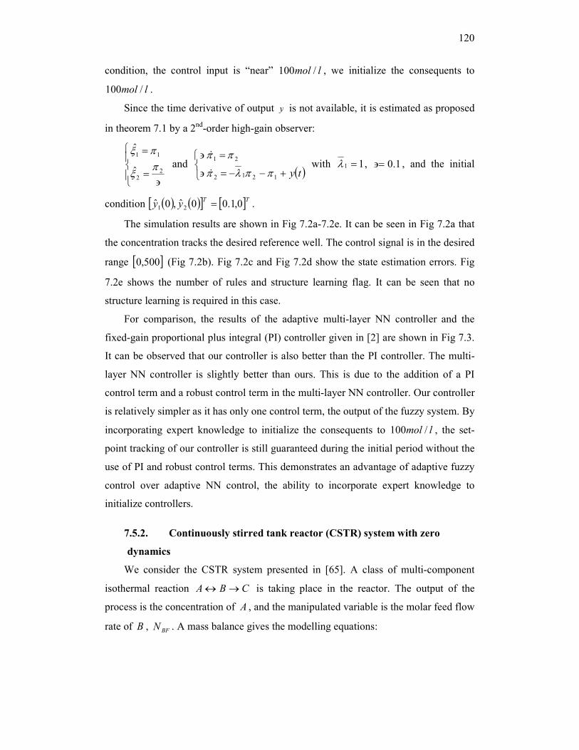
120
condition, the control input is “near” lmol /100 , we initialize the consequents to
lmol /100 .
Since the time derivative of output y is not available, it is estimated as proposed
in theorem 7.1 by a 2nd
-order high-gain observer:
∋=
=
22
11
ˆ
ˆ
πξ
πξ and
( )
+−−=∋
=∋
ty1212
21
ππλπ
ππ
&
& with 11 =λ , 1.0∋= , and the initial
condition ( ) ( )[ ] [ ]TTyy 0,1.00ˆ,0ˆ
21 = .
The simulation results are shown in Fig 7.2a-7.2e. It can be seen in Fig 7.2a that
the concentration tracks the desired reference well. The control signal is in the desired
range [ ]500,0 (Fig 7.2b). Fig 7.2c and Fig 7.2d show the state estimation errors. Fig
7.2e shows the number of rules and structure learning flag. It can be seen that no
structure learning is required in this case.
For comparison, the results of the adaptive multi-layer NN controller and the
fixed-gain proportional plus integral (PI) controller given in [2] are shown in Fig 7.3.
It can be observed that our controller is also better than the PI controller. The multi-
layer NN controller is slightly better than ours. This is due to the addition of a PI
control term and a robust control term in the multi-layer NN controller. Our controller
is relatively simpler as it has only one control term, the output of the fuzzy system. By
incorporating expert knowledge to initialize the consequents to lmol /100 , the set-
point tracking of our controller is still guaranteed during the initial period without the
use of PI and robust control terms. This demonstrates an advantage of adaptive fuzzy
control over adaptive NN control, the ability to incorporate expert knowledge to
initialize controllers.
7.5.2. Continuously stirred tank reactor (CSTR) system with zero
dynamics
We consider the CSTR system presented in [65]. A class of multi-component
isothermal reaction CBA →↔ is taking place in the reactor. The output of the
process is the concentration of A , and the manipulated variable is the molar feed flow
rate of B , BFN . A mass balance gives the modelling equations:

121
( )
A
BCC
BFBBBB
BAAAA
Cy
CVkFCtd
dCV
NCVkCVkFCtd
dCV
CVkCVkCCFtd
dCV
f
=
+−=′
+−−−=′
+−−=′
2
3
2
3
2
1
2
21
With the dimensionless variables given in table 7.2, we can obtain the
dimensionless state-space model description:
1
2
2333
2
23
2
221122
2
221111 1
xy
xcxx
uxcxcxcxx
xcxcxx
=
+−=
+−−+−=
+−−=
&
&
&
It is easy to check that the relative degree of this system is 2. Using the
transformation given in 7.2.1, the system can be transformed into
( ) ( )tfc
ugf
3
2102102
21
,,
+−=
+=
=
ηη
ξξξξξ
ξξ
&
&
&
where
( )[ ] 2211 11 ccf t −++= ξξ,
( ) ( ) ( )[ ] ttt ffccccfccf 32221121210 1212, ++−+−= ξξξξ ,
( ) tfcg 2210 2, =ξξ . Also, the Damkholer numbers are assumed as follows: 201 =c ,
1.02 =c , and 103 =c . Now, we can use the output feedback SSDAFC in theorem 7.1
to control this system.
For comparison purposes, we choose the same control objective as in [65]. The
control objective is to make the concentration AC track the set-point ( )tr of 02.0±
about the nominal product concentration of 1.0 . The initial conditions are chosen as
the nominal operating conditions [ ]Tx 110,3.3,1.00 = .
The control input is chosen as ( )10.7 :
( ) ( )∑=
==M
j
jjac XXuu1
ˆˆˆ ζθθ in which [ ]TvX ˆ,ˆ,ˆˆ21 ξξ= .
The operating variable ranges are chosen as follows:

122
[ ]15.0,05.01 ∈ξ ; [ ]05.0,05.02 −∈ξ ; [ ]8.0,8.0−∈v .
The controller parameters are chosen as follows:
[ ]Tk 101= ;
=
100
010Q ;
=
15
1551P ; 1000=γ ;
0=Lu ; 500=Uu .
The structure-learning parameters are as follows:
5.00 =ε , 5.1_ =thresholderror , max_mf_distance [ ]6.11.01.0= ,
min_mf_distance [ ] 4/6.11.01.0= , , 50=rulesB .
The initial fuzzy system has 8 rules with 2 membership functions in each input
dimension as shown in fig 7.4a-7.4c. Using the expert knowledge that at nominal
condition, the control input is “near” 100 , we initialize the consequents to 100 .
Since the time derivative of output y is not available, it is estimated as proposed
in theorem 7.1 by a 2nd
-order high-gain observer:
∋=
=
22
11
ˆ
ˆ
πξ
πξ and
( )
+−−=∋
=∋
ty1212
21
ππλπ
ππ
&
& with 11 =λ , 1.0∋= , and the initial
condition ( ) ( )[ ] [ ]TTyy 0,1.00ˆ,0ˆ
21 = .
The simulation results are shown in Fig 7.5a-7.5g. It can be seen in Fig 7.5a that
the concentration tracks the desired reference well. The control signal is in the desired
range [ ]500,0 (Fig 7.5b). Fig 7.5c and Fig 7.5d show the state estimation errors. Fig
7.5e shows the number of rules and structure learning flag. It can be seen that no
structure learning is required in this case. Fig 7.5f shows the internal dynamics. It can
be seen that the internal dynamics is stable.
The tracking performance obtained in [65] is given in Fig 7.6. It can be seen that
both Ge’s controller and our controller are successful. Ge’s controller responds faster.
This maybe due to the addition of an a priori control term based on a nominal model
and a bounding control term. Our controller is relatively simpler as it has only one
control term, the output of the fuzzy system. Also, Ge’s controller requires 500
neurons, whereas our controller requires only 8 rules.
7.5.3. Third-order system in triangular form )3.7(
A third-order system is given in [2] as:
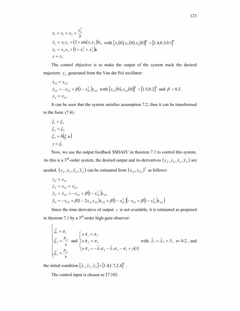
123
( )( )( )
1
2
2
2
1323
321212
3
2211
1
sin2
5
xy
uxxxxx
xxxxxx
xxxx
=
+++=
++=
++=
&
&
&
with ( ) ( ) ( )[ ] [ ]TTxxx 1.0,3.0,4.10,0,0 321 = .
The control objective is to make the output of the system track the desired
trajectory dy generated from the Van der Pol oscillator:
( )1
2
2
112
21
1
dd
dddd
dd
xy
xxxx
xx
=
−+−=
=
β&
&
with ( ) ( )[ ] [ ]TT
dd xx 2.0,5.10,0 21 = and 2.0=β .
It can be seen that the system satisfies assumption 7.2, thus it can be transformed
to the form )4.7( :
( )1
3
32
21
,
ξ
ξξ
ξξ
ξξ
=
=
=
=
y
ub&
&
&
Now, we use the output feedback SSDAFC in theorem 7.1 to control this system.
As this is a 3rd
-order system, the desired output and its derivatives ( )dddd yyyy &&&&&& ,,, are
needed. ( )dddd yyyy &&&&&& ,,, can be estimated from ( )Tdd xx 21 , as follows:
( )( ) ( ) ( )( )2
2
11
2
12212
2
2
112
21
1
1121
1
ddddddddd
ddddd
ddd
dd
xxxxxxxxy
xxxxy
xxy
xy
−+−−+−+−=
−+−==
==
=
βββ
β
&&&
&&&
&
Since the time derivative of output y is not available, it is estimated as proposed
in theorem 7.1 by a 3rd
-order high-gain observer:
∋=
∋=
=
23
22
11
ˆ
ˆ
ˆ
πξ
πξ
πξ
and
( )
+−−−=∋
=∋
=∋
ty122313
32
21
ππλπλπ
ππ
ππ
&
&
&
with 321 == λλ , 2.0∋= , and
the initial condition [ ] [ ]Tyyy 4.2,7.1,4.1ˆ,ˆ,ˆ321 = .
The control input is chosen as ( )10.7 :

124
( ) ( )∑=
==M
j
jjac XXuu1
ˆˆˆ ζθθ in which [ ]TvX ˆ,ˆ,ˆˆ21 ξξ= .
The operating variable ranges are chosen as follows:
[ ]5,51 −∈ξ ; [ ]3,32 −∈ξ ; [ ]3,33 −∈ξ [ ]3,3−∈v .
The controller parameters are chosen as follows:
[ ]Tk 10505= ;
=
1000
0100
0010
Q ;
=
72.017.210
17.258.4759.103
1059.10386.510
P ; 50=γ ;
50−=Lu ; 50=Uu .
The structure-learning parameters are as follows:
5.00 =ε , 5.2_ =thresholderror , max_mf_distance [ ]66610=
min_mf_distance [ ] 5/66610= , 200=rulesB .
The initial fuzzy system has 16 rules with 2 membership functions in each input
dimension as shown in fig 7.7a-7.7b. All the consequents are initialized to 0.
The simulation results are given in Fig 7.8. It can be seen in Fig 7.8a that the
output tracks the reference signal well. The control signal is in the range [ ]50,50− .
The actual states and their estimations are shown in Fig 7.8c-7.8e. the number of rules
and structuring flag is shown in Fig 7.8f. It can be seen that the final fuzzy controller
has 54 rules. The final membership functions of 1ξ , 2ξ , 3ξ , v are shown in Fig 7.9.
Compared to the adaptive NN controller proposed in [2], our controller has
similar performance. However, our controller requires only 1 fuzzy system with 54
rules, whereas the adaptive NN controller requires 3 neural networks (64 nodes, 256
nodes, 1024 nodes). Moreover, the adaptive NN controller also requires calculations
of some partial derivatives, which increase the complexity of the controller.
7.6. Conclusion
In this chapter, we extend the control scheme in chapter 6 to two broader classes
of nonlinear systems:
( )xhy
uxfx
=
= ),(,
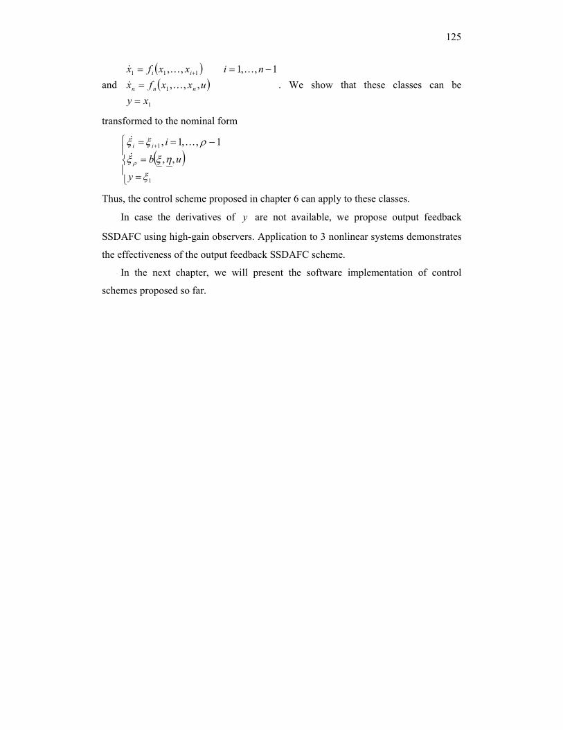
125
and
( )( )
1
1
111
,,,
1,,1,,
xy
uxxfx
nixxfx
nnn
ii
=
=
−== +
K&
KK&
. We show that these classes can be
transformed to the nominal form
( )
=
=
−== +
1
1
,,
1,,1,
ξ
ηξξ
ρξξ
ρ
y
ub
iii
&
K&
Thus, the control scheme proposed in chapter 6 can apply to these classes.
In case the derivatives of y are not available, we propose output feedback
SSDAFC using high-gain observers. Application to 3 nonlinear systems demonstrates
the effectiveness of the output feedback SSDAFC scheme.
In the next chapter, we will present the software implementation of control
schemes proposed so far.

126
0 10 20 30 40 50 60
0.08
0.09
0.1
0.11
0.12
0.13
concentration(m
ol/l)
Time(min)
actual output
desired ouput
Fig 7.2a: output tracking
0 0.02 0.04 0.06 0.08 0.1 0.12 0.14 0.16 0.18 0.2
0
0.2
0.4
0.6
0.8
1
input1D
egre
e o
f m
em
bers
hip
mf1 mf2
Fig 7.1a: membership functions for 1ξ
-0.5 -0.4 -0.3 -0.2 -0.1 0 0.1 0.2 0.3 0.4 0.5
0
0.2
0.4
0.6
0.8
1
input2
Degre
e o
f m
em
bers
hip
mf1 mf2
Fig 7.1b: membership functions for 2ξ
-1 -0.8 -0.6 -0.4 -0.2 0 0.2 0.4 0.6 0.8 1
0
0.2
0.4
0.6
0.8
1
input3
Degre
e o
f m
em
bers
hip
mf1 mf2
7.1c: membership functions for v
0 10 20 30 40 50 6085
90
95
100
105
110
115
120
coola
nt flow
rate
(l/m
in)
Time(min)
Fig 7.2b: control signal

127
0 10 20 30 40 50 60-0.03
-0.02
-0.01
0
0.01
0.02
0.03
0.04
(mol/l)
Time(min)
Fig 7.2c: state estimation error 11 ξ−x
0 10 20 30 40 50 60-0.1
-0.08
-0.06
-0.04
-0.02
0
0.02
0.04
0.06
0.08
(mol/l.m
in)
Time(min)
Fig 7.2d: state estimation error 121 ξ−x&
0 10 20 30 40 50 607
7.5
8
8.5
9
Num
ber of ru
les
Time(second)
0 10 20 30 40 50 600
0.5
1
1.5
2
Time(second)
Self-s
tructu
ring fla
g
Fig 7.2e: number of rules and structure learning flag

128
0.05 0.06 0.07 0.08 0.09 0.1 0.11 0.12 0.13 0.14
0
0.2
0.4
0.6
0.8
1
input1
Degre
e o
f m
em
bers
hip
mf1 mf2
Fig 7.4a: membership functions for
1ξ
Fig 7.3: results of Ge’s adaptive multi-layer NN controller and fixed-gain proportional plus integral (PI) controller

129
-0.05 -0.04 -0.03 -0.02 -0.01 0 0.01 0.02 0.03 0.04 0.05
0
0.2
0.4
0.6
0.8
1
input2
Degre
e o
f m
em
bers
hip
mf1 mf2
Fig 7.4b: membership functions for 2ξ
-0.8 -0.6 -0.4 -0.2 0 0.2 0.4 0.6 0.8
0
0.2
0.4
0.6
0.8
1
input3
Degre
e o
f m
em
bers
hip
mf1 mf2
Fig 7.4c: membership functions for v
0 20 40 60 80 100 120
0.08
0.09
0.1
0.11
0.12
0.13
The c
oncentration o
f A
Time
actual output
desired ouput
Fig 7.5a: output tracking
0 20 40 60 80 100 12060
70
80
90
100
110
120
130
140
150
160
The m
ola
r fe
edflow
rate
of B
Time
Fig 7.5b: control signal
0 20 40 60 80 100 120-0.1
-0.08
-0.06
-0.04
-0.02
0
0.02
0.04
0.06
0.08
0.1
Time
Fig 7.5c: state estimation error 11 ξ−x
0 20 40 60 80 100 120-0.1
-0.08
-0.06
-0.04
-0.02
0
0.02
0.04
0.06
0.08
0.1
Time
Fig 7.5d: state estimation error 121 ξ−x&

130
0 20 40 60 80 100 1207
7.5
8
8.5
9
Num
ber of ru
les
Time
0 20 40 60 80 100 1200
0.5
1
1.5
2
Time
Self-s
tructu
ring fla
g
Fig 7.5e: number of rules and structure learning flag
0 20 40 60 80 100 120-20
0
20
40
60
80
100
120
140
160
Time
Fig 7.5f: internal state η
Fig 7.6: tracking performance given in Ge and Jhang’s
-5 -4 -3 -2 -1 0 1 2 3 4 5
0
0.2
0.4
0.6
0.8
1
input1
Degre
e o
f m
em
bers
hip
mf1 mf2
Fig 7.7a: membership functions for variable 1ξ
-3 -2 -1 0 1 2 3
0
0.2
0.4
0.6
0.8
1
input2
Degre
e o
f m
em
bers
hip
mf1 mf2
Fig 7.7b: membership functions for variable 2ξ ,
3ξ , v

131
0 5 10 15 20 25 30-2.5
-2
-1.5
-1
-0.5
0
0.5
1
1.5
2
2.5
3
Time
actual output
desired ouput
Fig 7.8a: output
0 5 10 15 20 25 30-30
-20
-10
0
10
20
30
The m
ola
r fe
edflow
rate
of B
Time
Fig 7.8b: control signal
0 5 10 15 20 25 30-2.5
-2
-1.5
-1
-0.5
0
0.5
1
1.5
2
2.5
Time
Fig 7.8c: 1ξ (-) and
1ξ (- -)
0 5 10 15 20 25 30-5
-4
-3
-2
-1
0
1
2
3
Time
Fig 7.8d: 2ξ (-) and
2ξ
0 5 10 15 20 25 30-50
-40
-30
-20
-10
0
10
20
30
Time
Fig 7.8e: 3ξ (-) and
3ξ (- -)
0 5 10 15 20 25 300
20
40
60
Num
ber of ru
les
Time
0 5 10 15 20 25 30
-1
-0.5
0
0.5
1
Time
Self-s
tructu
ring fla
g
Fig 7.8f: number of rules and structuring flag

132
-5 -4 -3 -2 -1 0 1 2 3 4 5
0
0.2
0.4
0.6
0.8
1
input1
Degre
e o
f m
em
bers
hip
mf1 mf2mf3
Fig 7.9a: final membership functions for variable 1ξ
-3 -2 -1 0 1 2 3
0
0.2
0.4
0.6
0.8
1
input2
Degre
e o
f m
em
bers
hip
mf1 mf2mf3
Fig 7.9b: final membership functions for variable 2ξ
-3 -2 -1 0 1 2 3
0
0.2
0.4
0.6
0.8
1
input3
Degre
e o
f m
em
bers
hip
mf1 mf2mf3
Fig 7.9c: final membership functions for variable 3ξ
-3 -2 -1 0 1 2 3
0
0.2
0.4
0.6
0.8
1
input4
Degre
e o
f m
em
bers
hip
mf1 mf2
Fig 7.9d: final membership functions for variable v
133
8. Chapter 8
MATLAB IMPLEMENTATION
8.1. Introduction
Matlab and Simulink are integrated software packages that maybe used for
modeling, simulating, and analyzing dynamic systems. Simulink provides a graphical
user interface (GUI) for building models as block diagrams, using click-and-drag
mouse operations. It is a powerful tool for Simulation and Model-Based Design.
Simulink applications range from control design, signal processing and
communications, image processing, etc. [97].
In control design area, designers use Simulink and add-on products to design and
create software that is used in aerospace, defense, automotive, industrial equipment,
process control, and many other applications. Thus, Simulink is a very suitable tool to
implement our control algorithms.
In this chapter, we present the software implementation of our proposed control
algorithms. Programming issues are discussed in section 8.2. Section 8.3 presents our
Adaptive Fuzzy Control simulink library, which includes a DAFC block, a SSDAFC
block, and a high-gain observer block. Then, the simulation process is explained
through an example of controlling an inverted pendulum. Real-time control is
discussed in section 8.5.
8.2. Programming
The implementation of the developed control algorithms required extensive
coding of programs and functions. All of the programs and functions were written
using M-language (Matlab script). Custom fuzzy functions also had to be developed
as the standard Matlab fuzzy toolbox is not sufficient. All Simulink blocks were built
using 2-level M-file S-function template. For clarity, details of the written programs
and blocks will not be presented here. We would like to emphasize on the practical
use of the developed software.
Next, we will describe the available controller blocks and how to use them for
simulation and real time control of dynamic systems.

134
8.3. Adaptive Fuzzy Control simulink library
Fig 8.1 shows the developed Adaptive Fuzzy Control simulink library, which is
ready to be used for control applications. By dragging these blocks to a simulink
window, and connect them with a plant (represented by another simulink block), we
have a control application ready for simulation. The simulation process will be
presented in more detail in section 8.4.
8.3.1. DAFC block
Function:
This block implements the fixed-structured direct adaptive fuzzy controller
proposed in theorem 4.1.
Input:
There are two inputs: the state vector x and the desired output vector r .
( ) ( )( )1
21 ,,,,,, −== n
n yyyxxxx K&K
( )( )1,,, −= nrrrr K&
Output:
The output is the control signal generated by the controller.
Fig 8.1: Adaptive Fuzzy Control simulink library.

135
Parameters:
There are 8 parameters for this controller. These parameters are loaded to the
workspace by running the m file “parameters_DAFC.m”.
The code of this file is:
%==========================================================% % Parameters of the direct adaptive fuzzy controller % %==========================================================% % System order n=2;
%===============load fuzzy controller======================= fuzzy_u=readfis('fuzzy_system_1');
% ==============parameters k, A, Q, bc====================== k=[1;1]; A=[0 1;-k(1) -k(2)]; Q=[20 0;0 10]; bc=[0;1];
%===============adaptive law's parameters================== AFS_params.gamma=25; AFS_params.theta_U=25; AFS_params.theta_L=-25;
The meaning of the 8 parameters are:
• n: defines the system order.
• fuzzy_u: defines the initial fuzzy controller.
The initial fuzzy system is built using the Matlab fuzzy toolbox and saved to
hard-drive under the name “fuzzy_system_1”. When we run the m file
“parameters_DAFC.m”, “fuzzy_system_1” will be loaded as the initial fuzzy
controller. By changing the name of the file to be loaded (e.g. “fuzzy_system_2”, or
“fuzzy_system_3”), we can specify different fuzzy systems as the initial fuzzy
controller.
• k: defines vector k in equation ( )1.4 .
• A: defines matrix CΛ in equation ( )6.4 .
• Q: defines matrix Q in equation )7.4( .
• bc: defines vector Cb in equation ( )6.4 .
• AFS_params.sigma: defines the adaptive gain γ in equation ( )8.4 .

136
• AFS_params.theta_U: defines Uu in assumption 4.3 and equation
( )8.4 .
• AFS_params.theta_L: defines Lu in assumption 4.3 and equation
( )8.4 .
8.3.2. SSDAFC block
Function:
This block implements the self-structuring direct adaptive fuzzy controller
proposed in theorems 5.1 and 6.1.
Input:
There are two inputs: the state vector x and the desired output vector r .
( ) ( )( )1
21 ,,,,,, −== n
n yyyxxxx K&K
( )( )1,,, −= nrrrr K&
Output:
The output is the control signal generated by the controller.
Parameters:
The parameters can be loaded to the workspace by running the file
“parameters_SSDAFC.m”.
The code of this file is:
%==========================================================% % Parameters of the self-structuring direct adaptive fuzzy controller % %==========================================================% % System order n=2;
%===============load fuzzy controller======================= fuzzy_u=readfis('fuzzy_system_1');
% ==============parameters k, A, Q, bc====================== k=[1;1]; A=[0 1;-k(1) -k(2)]; Q=[20 0;0 10]; bc=[0;1];
%===============adaptive law's parameters================== AFS_params.gamma=25; AFS_params.theta_U=25; AFS_params.theta_L=-25; %===========Structure Learning parameters=================% structure_learning_params.max_N_rules = 125;

137
structure_learning_params.mf_threshold = 0.5; structure_learning_params.error_threshold = 5; structure_learning_params.a0 = [2.5 7.5 10]; structure_learning_params.center_distance_threshold = [1 15/5 20/5];
The first 8 parameters have the same meaning as the ones in the DAFC block.
The additional 5 parameters are for the self-structuring algorithm. Their meanings are:
• structure_learning_params.max_N_rules: defines ruleB in assumption
5.1 and assumption 6.3.
• structure_learning_params.mf_threshold: defines the completeness of
fuzzy rules 0ε .
• structure_learning_params.error_threshold: defines the minimum level
of error to trigger structure change thresholderror _ .
• structure_learning_params.a0: defines max_mf_distance, i.e. the
maximum allowed distance between two neighbouring membership
functions.
• structure_learning_params.center_distance_threshold: defines
min_mf_distance, i.e. the minimum allowed distance between two
neighbouring membership functions.
8.3.3. High-gain observer block
Function:
This block implements the high gain observer given in lemma 7.1.
Input:
The input is the output y of the controlled plant.
Output:
The output is the estimated state vector ( )nxxxx ˆ,,ˆ,ˆˆ21 K= .
Paramters:
The parameters are loaded to the workspace by running the m file
“observer_parameters.m”.
The code of the file “observer_parameters.m” is:\
%=========================================% % High-gain observer parameters % %=========================================% lamda_vector = 2; % defines vector lamda epsilon = 0.5; % defines parameter epsilon

138
Their meanings are:
• lamda_vector: defines vector ( )Tn 121 ,,, −= λλλλ K in lemma 7.1.
• epsilon: defines ∋ in lemma 7.1
8.4. AFC simulation
This section presents how an AFC simulation is created and simulated. The
simulation process has four steps. This will be presented through an example of
controlling an inverted pendulum. Assuming that the state variables are available for
measurement, we will employ the fixed-structured DAFC block.
8.4.1. Create a Simulink model for the AFC application
First, we create a new simulink model and add the block representing the inverted
pendulum as shown in Fig 8.2.
Then, drag the DAFC block from the AFC library to the new model and connect
with the inverted pendulum as shown in Fig 8.3. The sinusoidal reference signal is
generated by the “signal generator” block.
Fig 8.2: The created simulink model with an inverted pendulum block.

139
To observe the control signal and the output of the inverted pendulum, Scope1 and
Scope2 are added as shown in Fig 8.4.
8.4.2. Design the fuzzy system that is used as the initial controller
The Matlab fuzzy toolbox is used to create the initial fuzzy controller. This fuzzy
toolbox allows users to easily create a fuzzy system through its Graphical User
Interface (GUI) as demonstrated in Fig 8.5.
As all possible rules are used, it is sometime impractical to add rules one by one,
especially for a large number of rules (>50). We have created a script
“generate_rules.m” to help add all the possible rules to a fuzzy system. By using the
Matlab comment:
fuzzy_system1 = generate_fis(fuzzy_system1,b),
we add all the possible rules to fuzzy_system1 and initialize them to value b.
Fig 8.4: Simulink model after added scope1 and scope2.
Fig 8.3: Simulink model after the DAFC block and Signal Generator block are added.

140
8.4.3. Load the controller’s parameters
Specify the controller’s parameters in the m file “parameters_DAFC.m” (see
section 8.3.1) and run it to load the controller’s parameters to the workspace.
8.4.4. Perform simulation
Now, the model is ready for simulation. The simulation results are obtained by
simply running the model and observing the results through the scopes. The controller
can be tested with different parameters by repeating steps 8.4.2 to 8.4.4.
We have demonstrated the implementation process of DAFC of an inverted
pendulum using Simulink. The process is quick and easy with 4 simple steps. A
SSDAFC simulation of an inverted pendulum can be created by following the same
steps. Fig 8.6 shows a simulink model of a SSDAFC of an inverted pendulum with
the use of a high-gain observer.
Fig 8.5: Fuzzy logic GUIs: The Membership Function Editor (top left), FIS Editor (center), Rule Editor (top right), Rule
Viewer (bottom left), and Surface Viewer (bottom right). Click on image to see enlarged view.

141
The blocks in the AFC library not only can be used for simulation but also for
real-time control. In the next section, we will show how a real-time control
application can be easily set-up using our control simulink blocks.
8.5. Real-time AFC
Real-Time Windows Target is an add-on product of Simulink. It enables running
of Simulink and Stateflow models in real time on a desktop or laptop PC for rapid
prototyping or hardware-in-the-loop simulation of a control system. Creation, control
, and real-time execution maybe done entirely through Simulink [98].
Real-Time Windows Target includes a set of I/O blocks that provide connections
between the physical I/O board and real-time model. The real-time windows target
library is shown in Fig 8.7.
Fig 8.6 Observer-based SSDAFC of an inverted pendulum

142
By configuring these blocks with the physical I/O board, the adaptive fuzzy
controller can be easily connected with the real physical plant. Fig 8.8 shows the setup
of a real-time observer-based SSDAFC of an inverted pendulum.
Fig 8.7 Real-time Windows Target library
Fig 8.8 Real-time observer-based SSAFC of an inverted pendulum.

143
8.6. Conclusion
In this chapter, we have presented Matlab/Simulink implementation of our
proposed control algorithms. A simulation application can be performed by only four
simple steps. A simulation can be converted to a real-time control implementation by
simply replacing the simulated plant by the I/O blocks provided in the real-time
windows target library.

144
9. Chapter 9
DISCUSSION AND CONCLUSION
9.1. Discussion
9.1.1. Main contributions
In this research, an online SSAFC scheme has been developed. The main features
of the proposed control scheme are:
• It is applicable for a number of different classes of continuous SISO
nonlinear systems
• It needs less restriction on the controlled plants
• The stability of the overall system, especially when the structure
changes, is guaranteed using the Lyapunov stability technique.
• The overall system is stable in the sense that all the variables are
bounded (including number of rules generated) and the tracking error
is uniformly ultimately bounded.
• For nonlinear systems in triangular forms, only one fuzzy system is
needed (unlike the back-stepping approach where one fuzzy system is
needed at each step).
The proposed control scheme makes practical application of AFC easier.
Designers need to specify only a few design parameters and no longer have to specify
the controller structure by trial and error. It saves the time and cost needed to check
the extra restrictions on the controlled plants. It greatly reduces the complexity for
nonlinear systems in triangular forms that are normally controlled using the back-
stepping approach. It guarantees the stability of the system at any time and also
guarantees that the fuzzy controller never exceeds the hardware capacity.
From the practitioners’ point of view, the ability of the control scheme to control
a wide range of classes of systems is a great advantage. When understanding the
method, designers do not have to worry about choosing the right control configuration
for a particular problem. This saves practitioners both learning time and designing
time.
The Matlab and Simulink implementation of the controllers make simulations
and real-time applications of AFC easy and fast. A simulation can be performed by

145
following four simple steps. Then, the simulation can be converted to a real-time
application by simply re-connecting the controller to the real-time plant.
9.1.2. Limitations
The developed self-structuring algorithm suffers “the curse of dimensionality”.
The number of added rules will dramatically increases for high-order systems. Thus, a
much larger hardware capacity is needed for controlling high-order systems.
The control scheme guarantees that all the signals are bounded. However, similar
to other AFC schemes, the bounds can be very conservative. Thus, information
regarding these bounds is generally not useful for selecting design parameters. The
control schemes in the literature suffer the same drawback. The reason is the bounds
depend on the quantity ∗θ where
∗θ is the ideal adaptive parameter vector. ∗θ
increases with the number of rules and can be arbitrarily large.
9.1.3. Future research
One future research direction would be to develop a self-structuring algorithm for
high-order systems. Instead of using all possible rules when a membership function is
added, we only add 1 rule at a time and all its corresponding memberships. The
change would reduce the interpretability of the fuzzy system. This is a trade-off
between computation and interpretability. However, as the system order increases, the
fuzzy rules are harder to interpret anyway.
Another future research direction would be to develop tighter bounds. The
popular way of proving the stability is to choose the Lyapunov function
( ) ( )∗∗ −−+= θθθθTT
ePeV2
1
2
1.
Thus, V depends on ∗θ , and therefore the bounds depend on
∗θ . If we choose a
new Lyapunov function
( )22
1
2
1 ∗−+= uuePeVT
new ,
then newV is much smaller than V . By investigating the approximation properties of
derivatives of fuzzy systems, we may find a way to establish the stability for newV .
Finally, a practical control problem generally includes selecting a suitable
actuator, a reference model, and a controller. The relationship between actuator
constraints, reference model, and AFC design parameters has not been thoroughly

146
investigated in the literature. It is of great practical interest to investigate how to
incorporate actuator constraints and reference signal information into the choice of
AFC design parameters. Understanding this would result in a more systematic design
procedure.
9.2. Conclusion
In conclusion, the objectives set at the beginning of the research are met. The
developed control scheme and implementation software make AFC easier. The results
also open new research challenges with the ultimate purpose being to make AFC an
easy-to-use control tool in practice.

147
Appendixes
Appendix 3.A
• Proof of 3.1(a.i) and 3.1(a.ii):
From the choice of the adaptive laws (3.3), (3.4), and (3.5), it is obvious that (a.i)
and (a.ii) holds. Now, we are going to prove (a.iii).
• Proof of 1(a.iii)
Substituting control signal (3.2) to system (3.1), we have:
Cn
n uxgxfyx )()()( +==&
Adding and subtracting Cguxg )(ˆ θ gives:
( ) ( )
( )( ) SgCg
f
Tn
SgnT
Cgfn
uxguxgxg
xfxfeke
uxgrek
uxgxgxfxfy
)(ˆ)()(ˆ
)()(ˆ
)(ˆ
)(ˆ)()(ˆ)(
)(
)(
)(
θθ
θ
θ
θθ
−−+
−+−=⇔
+++
−+−=
In the matrix form, we have:
( ) ( )[ ]SgCgfC
C
uxguxgxgxfxfb
ee
)(ˆ)()(ˆ)()(ˆ θθθ −−+−+
Λ=& (3.A.1)
The Lyapunov design approach will be used to prove the stability of the system.
Consider the following Lyapunov function
2
2
1
2
1
2
1
2
1)( ω
ωψ
γφφ
γφφ
γ+++=
g
T
gg
f
T
ff
TePetV (3.A.2)
in which *
fffθθφ −= , *
gggθθφ −= , and ωψ ω ˆ−=W .
Its derivative along the solution (3.A.1) is
ωωω
ψψγ
φφγ
φφγ
&&&& 111
2
1+++
∂∂
=g
T
gg
f
T
ff
TePe
tV (3.A.3)
Using the facts that ( ) TC
TTC ee Λ=Λ , ePbbPe
T
CC
T = , and QPP CT
C −=Λ+Λ .. , we
have:
( ) ( )[ ]SgCgfC
TTTuxguxgxgxfxfbPeeQeePe
t)(ˆ)()(ˆ)()(ˆ
2
1
2
1θθθ −−+−+−=
∂∂
Substituting to (3.A.3) gives

148
( ) ( )[ ]ωω
ωψψ
γφφ
γφφ
γ
θθθ
&&&
&
111
)(ˆ)()(ˆ)()(ˆ
2
1
+++
−−+−+
−=
g
T
gg
f
T
ff
SgCgfC
T
T
uxguxgxgxfxfbPe
eQeV
( ) ( )[ ]
( ) ( )[ ]SC
T
CgfC
T
g
T
gg
f
T
ff
CggffC
T
T
uxgbPe
uxgxgxfxfbPe
uxgxgxfxfbPe
eQe
)(ˆ
)()(ˆ)()(ˆ
111
)(ˆ)(ˆ)(ˆ)(ˆ
2
1
**
**
−
−+−+
+++
−+−+
−=
θθ
ψψγ
φφγ
φφγ
θθθθ
ωωω
&&& (3.A.4)
Now, considering the second and forth terms of (3.A.4), we have:
( )
f
T
ff
f
T
fCT
f
T
ff
ffCT
xbPe
xfxfbPe
φφγ
ζφ
φφγ
θθ
&
&
1)(
1)(ˆ)(ˆ *
+=
+−
Using the adaptive law (3.3), it is obvious that
01
)( ≤+f
T
ff
f
T
fC
TxbPe φφ
γζφ & (3.A.5)
Similarly, considering the third and fifth terms of (3.A.4), and the adaptive law
(3.4), we have
( )
01
)(
1)()(
*
≤+=
+−
g
T
gf
g
T
gC
T
g
T
gg
ggC
T
xbPe
xgxgbPe
φφγ
ζφ
φφγ
θθ
&
&
(3.A.6)
Considering the last three terms of (3.A.4) and using the adaptive law (3.5) and
the fact that εε
≤−ab
abba2785.0
tanh , we have
( ) ( )[ ]
( )( )( )
−>=+−
−≤=
<+−−
≤
+−
−+−
)ˆ( and ˆ if )ˆ(
)ˆ( and ˆor
ˆ if )ˆ)(ˆ(
1)(ˆ
)()(ˆ)()(ˆ
0max
0max
max0
**
ωωσωωεω
ωωσωω
ωωεωωωσ
ψψγ
θθ
ω
ωωω
CT
C
T
CT
SC
T
CgfC
T
PbeWbPe
Pbe
W
uxgbPe
uxgxgxfxfbPe
&

149
Moreover, we have that 0)( max ≤−ωWbPe CT and
200 )(
4
1)ˆ)(ˆ( ωσωωωσ ωω −≤−− WW . Therefore,
( ) ( )[ ]
)(4
1
1)(ˆ
)()(ˆ)()(ˆ
20
**
εωσ
ψψγ
θθ
ω
ωωω
+−≤
+−
−+−
W
uxgbPe
uxgxgxfxfbPe
SC
T
CgfC
T
& (3.A.7)
From (3.A.4-3.A.7), we have
εωσω +−+−≤ 20 )(
4
1
2
1WeQeV
T&
Let εωσω +−= 20 )(
4
1Wd . (3.A.8)
From(3.A.8),
( )
rgf
ff
ggf
fff
T
VePk
dP
Q
P
Q
P
QeP
P
Q
deQ
deQeV
+
+++−≤
+−−
−−
−−−≤
+−≤
+−≤
222
2
maxmin
22
max
min22
max
min
22
max
min2
max
max
min
2
min
2
1
2
1
2
1)(
2
1
)max()(
)(
2
1max
)(
)(
2
1
max)(
)(
2
1)(
)(
)(
2
1
)(2
1
2
1
ωω
ωωω
ψγ
φγ
φγ
λ
ψψλλ
γφφ
λλ
γ
φφλλ
γλ
λλ
λ
&
in which min
max
min
)(
)(k
P
Q=
λλ
(3.A.9)
)max(2
1max
2
1max
2
1
)(
2)(
2
1 222
min
max ωω
ψγ
φγ
φγλ
λ +++=g
ff
f
rQ
dPV (3.A.10)
And using the fact that )(2
1
2
1
2
1)(
2
1 222
2
max tVePg
ff
f
≥+++ ωωψ
γφ
γφ
γλ t∀ , we
have
( ) rr
r
VtkVVtV
VkVkV
+−−≤⇒
+−≤
)exp()0()( min
minmin&
(3.A.11)
Therefore,
( )rVVtV ),0(max)( ≤
Since tePePetVT ∀≥≥ )(
2
1
2
1)(
2
minλ , we have

150
( )
( ))(
),0(max2
),0(max)(2
1
min
2
min
P
VVe
VVeP
r
r
λ
λ
≤⇔
≤
This completes the proof of 3.1(a.iii)
• Proof of 3.1(a.iv)
Recall the definition of e :
erx
xryre
−=⇔
−=−=
Therefore,
( ))(
),0(max2
min0
P
VVr
erx
r
λ+≤
+≤
• Proof of 3.1(a.v)
From control (3.2),
ε
ωω
θ
θθ
ˆ2758.0tanhˆ
)(ˆ
1
)(ˆ
)(ˆ
1 )(
C
T
g
Tnf
g
bPe
xg
ekrxfxg
u
+
++≤
It is clear that
( ) ( )Lgg xgxg θθ ˆˆ ≥
( ) ( )
≤
U
f
L
fxfxfxf θθ ˆ,ˆmax)(ˆ
( )1rr
n ≤
( ))(
),0(max2
min P
VVe r
λ≤
maxˆ ωω ≤
1ˆ2758.0
tanh ≤ε
ωCT
bPe
Thus, 3.1(a.v) holds.
• Proof of 3.1(b)
From (3.A.11), ( ) rr VtkVVtV +−−≤ )exp()0()( min , we have
rt
VtV ≤∞→
)(lim

151
Since 2min
2
min )(2
1)(
2
1
2
1)( ePePePetV
T λλ ≥≥≥ ,
)(
2lim
)(2
1lim
min
2min
P
Ve
VeP
r
t
rt
λ
λ
≤⇔
≤
+∞→
∞→
This completes the proof of 3.1(b).
• Proof of 3.1(c)
From (3.A.8),
deQeVT +−≤
2
1&
Using the fact that 2min
2
min )(2
1)(
2
1
2
1eQeQeQe
T λλ ≥≥ , we have
deQV +−≤ 2min )(
2
1λ&
Rearranging terms and integrating, we have
∫∫
+−≤
tt
dtQ
d
Q
Vdte
)(
2
)(
2
minmin
2
λλ
&
Since V is bounded we find that
)(
21lim
min
2
Q
ddte
t
t
t λ≤∫∞→
So the RMS error is bounded by
)(
21lim
min
2
Q
ddte
tRMS
t
t λ≤= ∫∞→
Appendix 3.B
• Proof of theorem 3.2(a.i)
From (3.5), it is clear that theorem 3.2(a.i) holds.
• Proof of theorem 3.2(a.ii)
Consider the following Lyapunov function
21
2
1
2
1)( ω
ωψ
γ+= ePetV
T (3.B.1)
The derivative of 1V along the solution of (3.A.1) is

152
( ) ( )[ ]ωω
ωψψ
γ
θθ
&
&
1
)()(ˆ)()(ˆ2
1 001
+−
−+−+−=
SC
T
CgfC
TT
ubPe
uxgxgxfxfbPeeQeV
Using assumption 3.4 and the same arguments in (3.A.7), we have
( ) ( )[ ]
dW
ubPeuxgxgxfxfbPe SC
T
CgfC
T
=+−≤
+−−+−
εωσ
ψψγ
θθ
ω
ωωω
2
0
00
)(4
1
1)()(ˆ)()(ˆ &
Thus,
deQeVT +−≤
2
11&
Now, following the same procedure to prove theorem 3.1(a.iii), we can prove that
theorem 3.2(a.ii) holds
( ))(
),0(max2
min
11
P
VVe r
λ≤
where 2
minmax1 )max(
2
1
)(
2)(
2
1ω
ωψ
γλλ +=
Q
dPV r (3.B.2)
• Proof of theorem 3.2(a.iii) and theorem 3.2(a.iv):
Using the same arguments to proof theorem 3.1(a.iv) and theorem 3.1(a.v), we
can show that theorem 3.2(a.iii) and theorem 3.2(a.iv) hold.
• Proof of theorem 3.2(b):
Similar to the proof of theorem 3.1(b), from deQeVT +−≤
2
11& , we can show that
)(
2lim
min
1
P
Ve r
t λ≤
+∞→.
• Proof of theorem 3.2(c):
Using the same arguments as in the proof of theorem 3.1(c) and deQeVT +−≤
2
11& ,
we can conclude that
)(
2
min Q
dRMS
λ≤ .
Appendix 4.B
Let Xj
UX ∈ . As ( )xg , ( )θXu , and ( )Xu∗ are continuous at jX , for each
1,1 += nni K , there exists a 0>jiδ such that
153
( ) ( ) ( ) ( ) ( )[ ] ( ) ( ) ( ) ( )[ ] ∗∗∗ ≤−−−⇔+=<− εθθδ jjjjji
jii XuXgXuXgXuXgXuXgniXX ˆˆ11 K
( ) ( ) ( ) ( )[ ] ( ) ( ) ( )( ) ∗∗∗ ≤−−−⇔ εθθ jjjXuXuXgXuXgXuXg ˆˆ
( ) ( ) ( ) ( )[ ] ( ) ( )( ) ∗∗∗ ≤−−−⇔ εθθ jjj XuXucXuXgXuXg ˆˆ ( )1..4 A
where ( ) 0>= jj Xgc .
Define
( ) 11 +=≤−=Ο niXXXji
jiij Kδ
As XU is compact, there exists a finite subfamily 1Ο , 2Ο ,K , MΟ such that
MXU Ο∪∪Ο∪Ο⊆ K21
Choose
( ) ( )( )iji
ji
ji
jii
ji XXXXA δδα +−= , , 11 += ni K , Mj K1= such that
( )( ) Mkj
jkXA
jkXAki
ji
ki
ji K1, ,
if 0
if 1=
≠=
== ( )2..4 A
( )jj Xu∗∗ =θ , Mj K1= ( )3..4 A
From (A.2),
( ) ( ) jMj
M
k
jkk
jXXu θθθθθζθ =×++×+×+×==∑
=
0100ˆ 21
1
KK ( )4..4 A
Substituting (4.A.3) and (4.A.4) to (4.A.1), we have:
( ) ( ) ( ) ( )[ ] ( ) ∗∗∗ ≤−−− εθθθ jjjcXuXgXuXg ˆ ( )5..4 A
As ( ) jj XX Ο∈≠ for 0ζ and ( ) jj XX Ο∉= for 0ζ ,
( ) ( ) ( ) ( ) ( )[ ] ( ) ( ) ( )XXcXuXgXuXgA jjjjj ζεζθθθ ∗∗∗ ≤−−−⇒ ˆ5.
Take the summation for Mj K1= ,
( ) ( ) ( ) ( )[ ] ( ) ( ) ( )∑ ∑= =
∗∗∗ ≤−−−M
j
M
j
jjjjj XXcXuXgXuXg
1 1
ˆ ζεζθθθ
( ) ( ) ( ) ( )[ ] ( ) ( ) ( ) ( )∑∑∑=
∗
=
∗
=
∗ ≤−−−⇔M
j
j
M
j
jjjj
M
j
j XXcXXuXgXuXg111
ˆ ζεζθθζθ
Since ( ) 11
=∑=
M
j
j Xζ , we have:
( ) ( ) ( ) ( )[ ] ( ) ( ) ∗
=
∗∗ ≤−−− ∑ εζθθθM
j
jjjj XcXuXgXuXg
1
ˆ ( )6..4 A

154
Thus, ( ) ( ) ( ) ( )θXuxgXuxg ˆ−∗ can be approximated by ( ) ( )∑=
∗ −M
j
jjjj Xc
1
ζθθ :
( ) ( ) ( ) ( ) ( ) ( ) εζθθθ +−=− ∑=
∗∗M
j
jjjj XcXuxgXuxg
1
ˆ
where ∗≤ εε and jc are some positive constants.
Appendix 6.A
Let Xj
UX ∈ . Since ( )( )Xuxf , is continuous with respect to ( )Xu , according to the
Mean Value Theorem, there exists a positive constant 0>jc such that
( )( ) ( )( ) ( ) ( )( )jjjjjjjXuXucXuxfXuxf −=− ∗,, * ( )1..6 A
Since ( )( ) ( )( )jjjjXuxfXuxf ,, * − is continuous at j
X , for each 1,1 += nni K , there
exists 0>jiδ such that
( ) ( )( ) ( )( )[ ] ( )( ) ( )( )[ ] ∗∗∗ ≤−−−⇔+=<− εδ jjjjji
jii XuxfXuxfXuxfXuxfniXX ,,,,11 K
( )2..6 A
Substituting ( )1..6 A to ( )2..6 A gives
( ) ( )( ) ( )( )[ ] ( ) ( )( )[ ] ∗∗∗ ≤−−−⇔+=<− εδ jjjji
jii XuXucXuxfXuxfniXX ,,11 K ( )3..6 A
where 0>jc .
Define
( ) 11 +=≤−=Ο niXXXji
jiij Kδ
As XU is compact, there exist a finite subfamily 1Ο , 2Ο ,K , MΟ such that
MXU Ο∪∪Ο∪Ο⊆ K21
Choose
( ) ( )( )iji
ji
ji
jii
ji XXXXA δδα +−= , , 11 += ni K , Mj K1= such that
( )( ) Mkj
jkXA
jkXAki
ji
ki
ji K1, ,
if 0
if 1=
≠=
== ( )4..6 A
( )jj Xu∗∗ =θ , Mj K1= ( )5..6 A
From (6.A.4),
( ) ( ) jMj
M
k
jkk
jXXu θθθθθζθ =×++×+×+×==∑
=
0100 21
1
KK ( )6..6 A
Substituting ( )5..6 A and ( )6..6 A to ( )3..6 A , we have:

155
( ) ( )( ) ( )( )[ ] ( )[ ] ∗∗∗ ≤−−−⇔+=<− εθθδ jjjj
ijii cXuxfXuxfniXX ,,11 K ( )7..6 A
As ( ) jj XX Ο∈≠ for 0ζ and ( ) jj XX Ο∉= for 0ζ ,
( ) ( )( ) ( )( )[ ] ( ) ( ) ( )XXcXuxfXuxfA jjjj
j ζεζθθ ∗∗∗ ≤−−−⇒ ,,7..6
Take the summation for Mj K1= ,
( )( ) ( )( )[ ] ( ) ( ) ( )∑ ∑= =
∗∗∗ ≤−−−M
j
M
j
jjjjj
XXcXuxfXuxf
1 1
,, ζεζθθ
( )( ) ( )( )[ ] ( ) ( ) ( ) ( )∑∑∑=
∗
=
∗
=
∗ ≤−−−⇔M
j
j
M
j
jjjj
M
j
j XXcXXuxfXuxf
111
,, ζεζθθζ
Since ( ) 1
1
=∑=
M
j
j Xζ , we have:
( )( ) ( )( )[ ] ( ) ( ) ∗
=
∗∗ ≤−−− ∑ εζθθM
j
jjjj XcXuxfXuxf
1
,, ( )8..6 A
Thus, ( )( ) ( )( )XuxfXuxf ,, −∗ can be approximated by ( ) ( )∑=
∗ −M
j
jjjj
Xc
1
ζθθ :
( )( ) ( )( ) ( ) ( ) εζθθ +−=− ∑=
∗∗M
j
jjjj
XcXuxfXuxf
1
,,
where ∗≤ εε and jc are some positive constants.

156
References
[1] L.-X. Wang, Adaptive fuzzy systems and control: design and stability
anyalysis. New Jersey: Prentice-Hall: Englewood Cliffs, 1994.
[2] S. S. Ge, C. C. Hang, T. H. Lee, and T. Zhang, Stable adaptive neural network
control. London: Kluwer Academic Publishers, 2002.
[3] J. T. Spooner, M. Maggiore, R. Ordonez, and K. M. Passino, Stable adaptive
control and estimation for nonlinear systems: neural and fuzzy approximation
techniques. New York: John Wiley & Sons, 2002.
[4] J. T. Spooner and K. M. Passino, "Stable adaptive control using fuzzy systems
and neural networks," Ieee Transactions on Fuzzy Systems, vol. 4, pp. 339-
359, 1996.
[5] K. Fischle and D. Schroder, "An improved stable adaptive fuzzy control
method," Ieee Transactions on Fuzzy Systems, vol. 7, pp. 27-40, 1999.
[6] C. G. Moore and C. J. Harris, "Indirect Adaptive Fuzzy Control,"
International Journal of Control, vol. 56, pp. 441-468, 1992.
[7] Y. W. Cho, C. W. Park, and M. Park, "An indirect model reference adaptive
fuzzy control for SISO Takagi-Sugeno model," Fuzzy Sets and Systems, vol.
131, pp. 197-215, 2002.
[8] C. W. Park and Y. W. Cho, "T-S model based indirect adaptive fuzzy control
using online parameter estimation," Ieee Transactions on Systems Man and
Cybernetics Part B-Cybernetics, vol. 34, pp. 2293-2302, 2004.
[9] C. W. Park and M. Park, "Adaptive parameter estimator based on T-S fuzzy
models and its applications to indirect adaptive fuzzy control design,"
Information Sciences, vol. 159, pp. 125-139, 2004.
[10] L. X. Wang, "Combining mathematical model and heuristics into controllers:
An adaptive fuzzy control approach," Fuzzy Sets and Systems, vol. 89, pp.
151-156, 1997.
[11] M. Hojati and S. Gazor, "Hybrid adaptive fuzzy identification and control of
nonlinear systems," Ieee Transactions on Fuzzy Systems, vol. 10, pp. 198-210,
2002.
[12] M. J. Er and S. H. Chin, "Hybrid adaptive fuzzy controllers of robot
manipulators with bounds estimation," Ieee Transactions on Industrial
Electronics, vol. 47, pp. 1151-1160, 2000.
[13] C. H. Wang, T. C. Lin, T. T. Lee, and H. L. Liu, "Adaptive hybrid intelligent
control for uncertain nonlinear dynamical systems," Ieee Transactions on
Systems Man and Cybernetics Part B-Cybernetics, vol. 32, pp. 583-597, 2002.
[14] S. C. Tong and T. Y. Chai, "Fuzzy indirect adaptive control for a class of
decentralized nonlinear systems," International Journal of Systems Science,
vol. 29, pp. 149-157, 1998.
[15] B. Yoo and W. Ham, "Adaptive fuzzy sliding mode control of nonlinear
system," Ieee Transactions on Fuzzy Systems, vol. 6, pp. 315-321, 1998.
[16] S. C. Tong, T. Wang, and J. T. Tang, "Fuzzy adaptive output tracking control
of nonlinear systems," Fuzzy Sets and Systems, vol. 111, pp. 169-182, 2000.
[17] Y. C. Chang, "Adaptive fuzzy-based tracking control for nonlinear SISO
systems via VSS and H-infinity approaches," Ieee Transactions on Fuzzy
Systems, vol. 9, pp. 278-292, 2001.

157
[18] Y. X. Diao and K. M. Passino, "Stable fault-tolerant adaptive fuzzy/neural
control for a turbine engine," Ieee Transactions on Control Systems
Technology, vol. 9, pp. 494-509, 2001.
[19] C. L. Hwang and C. Y. Kuo, "A stable adaptive fuzzy sliding-mode control for
affine nonlinear systems with application to four-bar linkage systems," Ieee
Transactions on Fuzzy Systems, vol. 9, pp. 238-252, 2001.
[20] W. Y. Wang, Y. G. Leu, and C. C. Hsu, "Robust adaptive fuzzy-neural control
of nonlinear dynamical systems using generalized projection update law and
variable structure controller," Ieee Transactions on Systems Man and
Cybernetics Part B-Cybernetics, vol. 31, pp. 140-147, 2001.
[21] J. H. Park, S. J. Seo, and G. T. Park, "Robust adaptive fuzzy controller for
nonlinear system using estimation of bounds for approximation errors," Fuzzy
Sets and Systems, vol. 133, pp. 19-36, 2003.
[22] C. M. Lin and C. F. Hsu, "Adaptive fuzzy sliding-mode control for induction
servomotor systems," Ieee Transactions on Energy Conversion, vol. 19, pp.
362-368, 2004.
[23] Y. G. Leu, T. T. Lee, and W. Y. Wang, "Observer-based adaptive fuzzy-neural
control for unknown nonlinear dynamical systems," Ieee Transactions on
Systems Man and Cybernetics Part B-Cybernetics, vol. 29, pp. 583-591, 1999.
[24] A. Rubaai, "Direct adaptive fuzzy control design achieving H-infinity tracking
for high performance servo drives," Ieee Transactions on Energy Conversion,
vol. 14, pp. 1199-1208, 1999.
[25] T. Y. Chai and S. C. Tong, "Fuzzy direct adaptive control for a class of
nonlinear systems," Fuzzy Sets and Systems, vol. 103, pp. 379-387, 1999.
[26] B. S. Chen, C. S. Wu, and Y. W. Jan, "Adaptive fuzzy mixed H-2/H-infinity,
attitude control of spacecraft," Ieee Transactions on Aerospace and Electronic
Systems, vol. 36, pp. 1343-1359, 2000.
[27] W. Y. Wang, M. L. Chan, T. T. Lee, and C. H. Liu, "Adaptive fuzzy control
for strict-feedback canonical nonlinear systems with H-infinity tracking
performance," Ieee Transactions on Systems Man and Cybernetics Part B-
Cybernetics, vol. 30, pp. 878-885, 2000.
[28] S. C. Tong and H. X. Li, "Direct adaptive fuzzy output tracking control of
nonlinear systems," Fuzzy Sets and Systems, vol. 128, pp. 107-115, 2002.
[29] W. Y. Wang, M. L. Chan, C. C. J. Hsu, and T. T. Lee, "H-infinity tracking-
based sliding mode control for uncertain nonlinear systems via an adaptive
fuzzy-neural approach," Ieee Transactions on Systems Man and Cybernetics
Part B-Cybernetics, vol. 32, pp. 483-492, 2002.
[30] S. C. Tong, H. X. Li, and G. R. Chen, "Adaptive fuzzy decentralized control
for a class of large-scale nonlinear systems," Ieee Transactions on Systems
Man and Cybernetics Part B-Cybernetics, vol. 34, pp. 770-775, 2004.
[31] D. L. Tsay, H. Y. Chung, and C. J. Lee, "The adaptive control of nonlinear
systems using the Sugeno-type of fuzzy logic," Ieee Transactions on Fuzzy
Systems, vol. 7, pp. 225-229, 1999.
[32] C. H. Wang, H. L. Liu, and T. C. Lin, "Direct adaptive fuzzy-neural control
with state observer and supervisory controller for unknown nonlinear
dynamical systems," Ieee Transactions on Fuzzy Systems, vol. 10, pp. 39-49,
2002.
[33] J. H. Park and G. T. Park, "Robust adaptive fuzzy controller for non-affine
nonlinear systems with dynamic rule activation," International Journal of
Robust and Nonlinear Control, vol. 13, pp. 117-139, 2003.

158
[34] H. B. Du, H. H. Shao, and P. J. Yao, "Adaptive neural network control for a
class of low-triangular-structured nonlinear systems," Ieee Transactions on
Neural Networks, vol. 17, pp. 509-514, 2006.
[35] N. Essounbouli and A. Hamzaoui, "Direct and indirect robust adaptive fuzzy
controllers for a class of nonlinear systems," International Journal of Control
Automation and Systems, vol. 4, pp. 146-154, 2006.
[36] J. H. Park, S. H. Huh, S. H. Kim, S. J. Seo, and G. T. Park, "Direct adaptive
controller for nonaffine nonlinear systems using self-structuring neural
networks," Ieee Transactions on Neural Networks, vol. 16, pp. 414-422, 2005.
[37] J. H. Park, G. T. Park, S. H. Kim, and C. J. Moon, "Direct adaptive self-
structuring fuzzy controller for nonaffine nonlinear system," Fuzzy Sets and
Systems, vol. 153, pp. 429-445, 2005.
[38] A. J. Calise, N. Hovakimyan, and M. Idan, "Adaptive output feedback control
of nonlinear systems using neural networks," Automatica, vol. 37, pp. 1201-
1211, 2001.
[39] Y. H. Li, S. Qiang, X. Y. Zhuang, and O. Kaynak, "Robust and adaptive
backstepping control for nonlinear systems using RBF neural networks," Ieee
Transactions on Neural Networks, vol. 15, pp. 693-701, 2004.
[40] T. Zhang, S. S. Ge, and C. C. Hang, "Adaptive neural network control for
strict-feedback nonlinear systems using backstepping design," Automatica,
vol. 36, pp. 1835-1846, 2000.
[41] D. G. Chen and J. B. Yang, "Implementable adaptive backstepping neural
control of uncertain strict-feedback nonlinear systems," Advances in Neural
Networks - Isnn 2006, Pt 2, Proceedings, vol. 3972, pp. 875-880, 2006.
[42] Y. S. Yang, G. Feng, and J. S. Ren, "A combined backstepping and small-gain
approach to robust adaptive fuzzy control for strict-feedback nonlinear
systems," Ieee Transactions on Systems Man and Cybernetics Part a-Systems
and Humans, vol. 34, pp. 406-420, 2004.
[43] D. Wang and J. Huang, "Neural network-based adaptive dynamic surface
control for a class of uncertain nonlinear systems in strict-feedback form,"
Ieee Transactions on Neural Networks, vol. 16, pp. 195-202, 2005.
[44] S. S. Ge, C. C. Hang, and T. Zhang, "Adaptive neural network control of
nonlinear systems by state and output feedback," Ieee Transactions on Systems
Man and Cybernetics Part B-Cybernetics, vol. 29, pp. 818-828, 1999.
[45] S. S. Ge, J. Zhang, and T. H. Lee, "Adaptive neural network control for a class
of MIMO nonlinear systems with disturbances in discrete-time," Ieee
Transactions on Systems Man and Cybernetics Part B-Cybernetics, vol. 34,
pp. 1630-1645, 2004.
[46] J. Zhang, S. S. Ge, and T. H. Lee, "Output feedback control of a class of
discrete MIMO nonlinear systems with triangular form inputs," Ieee
Transactions on Neural Networks, vol. 16, pp. 1491-1503, 2005.
[47] C. Wang, D. J. Hill, S. S. Ge, and G. R. Chen, "An ISS-modular approach for
adaptive neural control of pure-feedback systems," Automatica, vol. 42, pp.
723-731, 2006.
[48] T. P. Zhang, "Stable direct adaptive fuzzy control for a class of MIMO non-
linear systems," International Journal of Systems Science, vol. 34, pp. 375-
388, 2003.
[49] R. Ordonez and K. M. Passino, "Stable multi-input multi-output adaptive
fuzzy neural control," Ieee Transactions on Fuzzy Systems, vol. 7, pp. 345-
353, 1999.

159
[50] N. Golea, A. Golea, and K. Benmahammed, "Fuzzy model reference adaptive
control," Ieee Transactions on Fuzzy Systems, vol. 10, pp. 436-444, 2002.
[51] Y. Gao and M. J. Er, "Online adaptive fuzzy neural identification and control
of a class of MIMO nonlinear systems," Fuzzy Systems, IEEE Transactions
on, vol. 11, pp. 462-477, 2003.
[52] H. X. Li and S. C. Tong, "A hybrid adaptive fuzzy control for a class of
nonlinear MIMO systems," Ieee Transactions on Fuzzy Systems, vol. 11, pp.
24-34, 2003.
[53] S. C. Tong and H. X. Li, "Fuzzy adaptive sliding-mode control for MIMO
nonlinear systems," Ieee Transactions on Fuzzy Systems, vol. 11, pp. 354-360,
2003.
[54] F. L. Lewis, S. Jagannathan, and A. Yeðsildirek, Neural network control of
robot manipulators and nonlinear systems. London: Taylor & Francis, 1999.
[55] S. S. Ge, T. H. Lee, and C. J. Harris, Adaptive Neural Network Control of
Robotic Manipulators. London: World Scientific, 1998.
[56] S. S. Ge, C. C. Hang, and T. Zhang, "Stable adaptive control for nonlinear
multivariable systems with a triangular control structure," Ieee Transactions
on Automatic Control, vol. 45, pp. 1221-1225, 2000.
[57] S. S. Ge and C. Wang, "Adaptive neural control of uncertain MIMO nonlinear
systems," Ieee Transactions on Neural Networks, vol. 15, pp. 674-692, 2004.
[58] S. Seshagiri and H. K. Khalil, "Output feedback control of nonlinear systems
using RBF neural networks," Ieee Transactions on Neural Networks, vol. 11,
pp. 69-79, 2000.
[59] F. Esfandiari and H. K. Khalil, "Output feedback stabilization of fully
linearizable system," Internation Journal of Control, vol. 56, 1992.
[60] M. Jankovic, "Adaptive output feedback control of nonlinear feedback
linearizable system," Internation Journal of Control, vol. 10, pp. 1-18, 1996.
[61] N. Hovakimyan, F. Nardi, and A. J. Calise, "A novel error observer-based
adaptive output feedback approach for control of uncertain systems," Ieee
Transactions on Automatic Control, vol. 47, pp. 1310-1314, 2002.
[62] Y. G. Leu, W. Y. Wang, and T. T. Lee, "Observer-based direct adaptive
fuzzy-neural control for nonaffine nonlinear systems," Ieee Transactions on
Neural Networks, vol. 16, pp. 853-861, 2005.
[63] N. Hovakimyan, A. J. Calise, and N. Kim, "Adaptive output feedback control
of a class of multi-input multi-output systems using neural networks,"
International Journal of Control, vol. 77, pp. 1318-1329, 2004.
[64] Y. C. Chang and H. M. Yen, "Adaptive output feedback tracking control for a
class of uncertain nonlinear systems using neural networks," Ieee Transactions
on Systems Man and Cybernetics Part B-Cybernetics, vol. 35, pp. 1311-1316,
2005.
[65] S. S. Ge and J. Zhang, "Neural-network control of nonaffine nonlinear system
with zero dynamics by state output feedback," Ieee Transactions on Neural
Networks, vol. 14, pp. 900-918, 2003.
[66] N. Hovakimyan, F. Nardi, A. Calise, and N. Kim, "Adaptive output feedback
control of uncertain nonlinear systems using single-hidden-layer neural
networks," Ieee Transactions on Neural Networks, vol. 13, pp. 1420-1431,
2002.
[67] S. Jagannathan, M. W. Vandegrift, and F. L. Lewis, "Adaptive fuzzy logic
control of discrete-time dynamical systems," Automatica, vol. 36, pp. 229-241,
2000.

160
[68] H. N. Nounou and K. M. Passino, "Stable Auto-Tuning of Adaptive
Fuzzy/Neural Controllers for Nonlinear Discrete-Time Systems," Fuzzy
Systems, IEEE Transactions on, vol. 12, pp. 70-83, 2004.
[69] S. S. Ge, T. H. Lee, G. Y. Li, and J. Zhang, "Adaptive NN control for a class
of discrete-time non-linear systems," International Journal of Control, vol. 76,
pp. 334-354, 2003.
[70] S. S. Ge, G. Y. Li, and T. H. Lee, "Adaptive NN control for a class of strict-
feedback discrete-time nonlinear systems," Automatica, vol. 39, pp. 807-819,
2003.
[71] S. S. Ge, G. Y. Li, J. Zhang, and T. H. Lee, "Direct adaptive control for a class
of MIMO nonlinear systems using neural networks," Ieee Transactions on
Automatic Control, vol. 49, pp. 2001-2006, 2004.
[72] M. Alata, C. Y. Su, and K. Demirli, "Adaptive control of a class of nonlinear
systems with a first-order parameterized Sugeno fuzzy approximator," Ieee
Transactions on Systems Man and Cybernetics Part C-Applications and
Reviews, vol. 31, pp. 410-419, 2001.
[73] H. Han, C.-Y. Su, and Y. Stepanenko, "Adaptive control of a class of
nonlinear systems with nonlinearly parameterized fuzzy approximators,"
Fuzzy Systems, IEEE Transactions on, vol. 9, pp. 315-323, 2001.
[74] J. H. Park, G. T. Park, S. H. Kim, and C. J. Moon, "Output-feedback control of
uncertain nonlinear systems using a self-structuring adaptive fuzzy observer,"
Fuzzy Sets and Systems, vol. 151, pp. 21-42, 2005.
[75] L. H. Tsoukalas and R. E. Uhrig, Fuzzy and Neural Approaches in
Engineering. New York: Willey, 1997.
[76] F. O. Karray and C. D. Silva, Soft Computing and Intelligent Systems Design:
theory, tools, and applications. New York: Pearson/Addison Wesley, 2004.
[77] M. Negnevitsky, Artificial Intelligence: a guide to intelligent systems. Harlow,
England: Addison Wesley, 2005.
[78] M. F. Alexander Fink*, Oliver Nelles‡, Rolf Isermann*, "Supervision of
nonlinear adaptive controllers based on fuzzy models," 2000.
[79] E. Kim, "Output feedback tracking control of robot manipulators with model
uncertainty via adaptive fuzzy logic," Ieee Transactions on Fuzzy Systems,
vol. 12, pp. 368-378, 2004.
[80] Y. X. Diao and K. M. Passino, "Adaptive neural/fuzzy control for interpolated
nonlinear systems," Ieee Transactions on Fuzzy Systems, vol. 10, pp. 583-595,
2002.
[81] Y. H. Park and G. T. Park, "Design of a robust adaptive fuzzy controller
globally stabilizing the multi-input nonlinear system with state-dependent
uncertainty," Control and Cybernetics, vol. 27, pp. 613-629, 1998.
[82] F. C. Sun, Z. Q. Sun, Y. Y. Zhu, and W. J. Lu, "Stable neuro-adaptive control
for robots with the upper bound estimation on the neural approximation
errors," Journal of Intelligent & Robotic Systems, vol. 26, pp. 91-100, 1999.
[83] F. C. Chen and C. C. Liu, "Adaptively Controlling Nonlinear Continuous-
Time Systems Using Multilayer Neural Networks," Ieee Transactions on
Automatic Control, vol. 39, pp. 1306-1310, 1994.
[84] Y. S. Yang and J. S. Ren, "Adaptive fuzzy robust tracking controller design
via small gain approach and its application," Ieee Transactions on Fuzzy
Systems, vol. 11, pp. 783-795, 2003.

161
[85] D. Velez-Diaz and Y. Tang, "Adaptive Robust Fuzzy Control of Nonlinear
Systems," Systems, Man and Cybernetics, Part B, IEEE Transactions on, vol.
34, pp. 1596-1601, 2004.
[86] F. P. Da and W. Z. Song, "Fuzzy neural networks for direct adaptive control,"
Ieee Transactions on Industrial Electronics, vol. 50, pp. 507-513, 2003.
[87] S. S. Ge and C. Wang, "Direct adaptive NN control of a class of nonlinear
systems," Ieee Transactions on Neural Networks, vol. 13, pp. 214-221, 2002.
[88] J. L. Castro, "Fuzzy-Logic Controllers Are Universal Approximators," Ieee
Transactions on Systems Man and Cybernetics, vol. 25, pp. 629-635, 1995.
[89] M. J. Er and S. Q. Wu, "A fast learning algorithm for parsimonious fuzzy
neural systems," Fuzzy Sets and Systems, vol. 126, pp. 337-351, 2002.
[90] F. J. Lin, C. H. Lin, and P. H. Shen, "Self-constructing fuzzy neural network
speed controller for permanent-magnet synchronous motor drive," Ieee
Transactions on Fuzzy Systems, vol. 9, pp. 751-759, 2001.
[91] C. F. Juang and C. T. Lin, "An on-line self-constructing neural fuzzy inference
network and its applications," Ieee Transactions on Fuzzy Systems, vol. 6, pp.
12-32, 1998.
[92] N. K. Kasabov and Q. Song, "DENFIS: Dynamic evolving neural-fuzzy
inference system and its application for time-series prediction," Ieee
Transactions on Fuzzy Systems, vol. 10, pp. 144-154, 2002.
[93] P. P. Angelov and D. P. Filev, "An approach to Online identification of
Takagi-Suigeno fuzzy models," Ieee Transactions on Systems Man and
Cybernetics Part B-Cybernetics, vol. 34, pp. 484-498, 2004.
[94] M. F. Azeem, M. Hanmandlu, and N. Ahmad, "Structure identification of
generalized adaptive neuro-fuzzy inference systems," Ieee Transactions on
Fuzzy Systems, vol. 11, pp. 666-681, 2003.
[95] J. H. Park and S. H. Kim, "Direct adaptive output-feedback fuzzy controller
for a nonaffine nonlinear system," Iee Proceedings-Control Theory and
Applications, vol. 151, pp. 65-72, 2004.
[96] J. H. Park, S. J. Seo, D. W. Kim, and G. T. Park, "Adaptive fuzzy output-
feedback controller for SISO affine nonlinear systems without state observer,"
in Knowledge-Based Intelligent Information and Engineering Systems, Pt 4,
Proceedings, vol. 3684, Lecture Notes in Artificial Intelligence, 2005, pp. 549-
558.
[97] "http://www.mathworks.com/products/simulink/."
[98] "htttp://www.mathworks.com/products/rtwt/."