a study of underground stormwater detention chambers and … · a study of underground stormwater...
TRANSCRIPT

A Study of Underground Stormwater Detention Chambers and
the Creation of the Model for Underground Detention of
Sediment
by
Nicholas David McIntosh
A thesis submitted in conformity with the requirements
for the degree of Master of Applied Science
Graduate Department of Civil Engineering
University of Toronto
© Copyright by Nicholas David McIntosh 2015

II
A Study of Underground Stormwater Detention Chambers and
the Creation of the Model for Underground Detention of
Sediment
Nicholas David McIntosh
Master of Applied Science
Graduate Department of Civil Engineering
University of Toronto
2015
Abstract
This thesis investigates the hydraulic and runoff treatment capabilities of Underground
Stormwater Detention Chambers (USDC) and compares them to stormwater management ponds,
the industry standard system for runoff detention and treatment. Runoff characteristics were
monitored at a USDC in Markham, Ontario. Characteristics include: total suspended solids,
turbidity, nutrients, metals, bacteria, temperature, and hydrocarbons. The Model for
Underground Detention of Sediment (MUDS) was created to predict the removal of suspended
solids by a USDC. The results indicate that the Markham USDC meets all provincial hydraulic
requirements and most water quality requirements. Also, the Markham USDC provides
equivalent or improved level of service compared to stormwater management ponds for runoff
treatment in most cases. MUDS was proven capable of accurately predicting USDC hydraulics
and suspended solids removal for both event based and continuous based simulations.

III
Acknowledgments
I would first like to thank Dr. Drake for her invaluable advice and guidance throughout the
preparation of this thesis. I would like to thank Jason Spencer (Con Cast Pipe), and Dean Young
and Tim Van Seters (Toronto and Region Conservation Authority) for answering my questions
and providing many helpful suggestions. Thanks and appreciation is also extended to Mark
Hummel and Jacob Kloeze (TRCA) for their field work. Lastly, I would like to thank my wife,
Ali, and parents, David and Brenda, for supporting and encouraging me throughout the years.

IV
Table of Contents
Acknowledgments ........................................................................................................................................ III
Table of Contents ......................................................................................................................................... IV
List of Tables ............................................................................................................................................... VI
List of Figures ............................................................................................................................................. VII
List of Symbols ............................................................................................................................................ IX
Chapter 1 Introduction .................................................................................................................................. 1
Chapter 2 Relevant Literature ....................................................................................................................... 6
2.1 Urbanization and Stormwater Management............................................................................................ 6
2.2 Stormwater Management Pond Pollutant Characteristics ....................................................................... 9
2.2.1 Total Suspended Solids .................................................................................................................... 9
2.2.2 Nutrients ......................................................................................................................................... 12
2.2.3 Heavy Metals ................................................................................................................................. 16
2.2.4 Temperature ................................................................................................................................... 20
2.2.5 First Flush ...................................................................................................................................... 21
2.2.6 Winter Conditions .......................................................................................................................... 22
2.3 Modeling of Stormwater Management Ponds....................................................................................... 23
2.3.1 K-C Decay Rate Model .................................................................................................................. 23
2.3.2 Sedimentation ................................................................................................................................ 24
2.3.3 Probabilistic ................................................................................................................................... 27
2.4 Summary ............................................................................................................................................... 28
Chapter 3 Methodology .............................................................................................................................. 30
3.1 Field Site ............................................................................................................................................... 30
3.2 Monitoring ............................................................................................................................................ 34
3.3 Water Quality Analysis ......................................................................................................................... 36
3.4 Modeling ............................................................................................................................................... 37
3.4.1 Hydraulics ...................................................................................................................................... 38
3.4.2 Particle Tracking ............................................................................................................................ 39
3.4.3 Pollutant Removal .......................................................................................................................... 41
3.4.5 SWMM Modeling .......................................................................................................................... 45
3.5 Summary ............................................................................................................................................... 48
Chapter 4 Water Quality Results ................................................................................................................ 50
4.1 Total Suspended Solids and Turbidity .................................................................................................. 51
4.2 Nutrients ................................................................................................................................................ 53

V
4.3 Metals .................................................................................................................................................... 56
4.4 Bacteria ................................................................................................................................................. 61
4.5 Temperature .......................................................................................................................................... 63
4.6 Hydrocarbons ........................................................................................................................................ 65
4.7 Vertical Profiles .................................................................................................................................... 67
4.8 Summary ............................................................................................................................................... 70
Chapter 5 Model Development and Results ............................................................................................... 73
5.1 SWMM Calibration and Validation ...................................................................................................... 75
5.2 Particle Removal Assessment ............................................................................................................... 80
5.2.1 Sensitivity Analysis ....................................................................................................................... 84
5.3 Markham USDC MUDS Simulations ................................................................................................... 85
5.3.1 Design Storm Simulation ............................................................................................................... 85
5.3.2 Continuous Simulation (May - Nov) ............................................................................................. 87
5.3.3 Seasonal Simulations ..................................................................................................................... 89
5.3.4 Sizing Simulations ......................................................................................................................... 90
5.4 Summary ............................................................................................................................................... 92
Chapter 6 Conclusions and Recommendations ........................................................................................... 95
6.1 Conclusions ........................................................................................................................................... 95
6.1.1 Objective 1 ..................................................................................................................................... 95
6.1.2 Objective 2 ..................................................................................................................................... 97
6.1.3 Objective 3 ..................................................................................................................................... 98
6.2 Recommendations for Future Research ................................................................................................ 99
6.2.1 Water Quality ................................................................................................................................. 99
6.2.2 Modeling ...................................................................................................................................... 100
6.2.3 USDC Design in Ontario ............................................................................................................. 101
References ................................................................................................................................................. 102
Appendix A: Layout of MUDS Interface ................................................................................................. 106
Appendix B: Removal Percentage Calculation ......................................................................................... 107
Appendix C: Hydrograph and Depth Figures of Storms used for Validation and Calibration of the SWMM
Model ........................................................................................................................................................ 113
VI
List of Tables
Table 1: TSS Removal Percentage by SWM .............................................................................................. 12 Table 2: Median Total and Soluble Phosphorus, Ammonia and Nitrate/Nitrite Concentrations by Land
Use .............................................................................................................................................................. 15 Table 3: Summary of Nitrogen and Phosphorus Transformations and Removal Mechanisms .................. 15 Table 4: Nutrient Removal Efficiency by SWM Ponds .............................................................................. 16 Table 5: Common Sources of Metal in Urban Runoff (Shaver et al., 2007) .............................................. 17 Table 6: Typical Levels of Metals Found in Stormwater Runoff (µg/L) .................................................... 17 Table 7: Percent Reduction in Metals after Removal of Various Particle Sizes ......................................... 18 Table 8: Percent Removal of Metals by SWM ........................................................................................... 19 Table 9: Metals Provincial Water Quality Requirements ........................................................................... 19 Table 10: Distribution of Event Constituents (EMC) ................................................................................. 28 Table 11: DoubleTrapTM Monitoring Equipment Properties and Purpose .................................................. 34 Table 12: Outflow Equations ...................................................................................................................... 38 Table 13: Particle Tracking Equations (Takamatsu et al., 2010) ................................................................ 40 Table 14: SWMM Subcatchment Properties .............................................................................................. 48 Table 15: SWMM Land Type Roughness and Storage .............................................................................. 48 Table 16: SWMM Conduit Properties ........................................................................................................ 48 Table 17: Sampled Storm Event Hydrologic Parameters ........................................................................... 50 Table 18: Summary of TSS EMC and Turbidity ........................................................................................ 51 Table 19: Summary of TSS and Turbidity Statistical Analysis .................................................................. 51 Table 20: Percent Removal of TSS and Turbidity ...................................................................................... 52 Table 21: Summary of Nutrient EMC ......................................................................................................... 54 Table 22: Summary of Nutrient Statistical Analysis................................................................................... 55 Table 23: Summary of Metals EMC ........................................................................................................... 57 Table 24: Summary of Metals Statistical Analysis ..................................................................................... 59 Table 25: Percent Removal of Metals ......................................................................................................... 61 Table 26: Summary of Bacteria EMC ......................................................................................................... 61 Table 27: Summary of Bacteria Statistical Analysis................................................................................... 62 Table 28: Number of Hydrocarbon Samples below the MDL .................................................................... 65 Table 29: Summary of Hydrocarbon Removal ........................................................................................... 66 Table 30: Hydrocarbon Provincial Water Quality Requirements ............................................................... 67 Table 31: Minimum Acceptable Dissolved Oxygen Concentration in Rivers for the Protection of Aquatic
Life (Canadian Council of Ministers of the Environment, 2015) ............................................................... 69 Table 32: Summary of Calibration and Validation Events ......................................................................... 73 Table 33: MUDS Input Values ................................................................................................................... 74 Table 34: Raw Inflow and Outflow Data Summary ................................................................................... 79 Table 35: TRCA and Average Monitored Storm PSD................................................................................ 82 Table 36: Assessment of Particle Removal Summary ................................................................................ 84 Table 37: Seasonal and Overall TSS Removal Simulation Results ............................................................ 89 Table 38: Summary of Forebay and Residence Time Significance Tests ................................................... 97

VII
List of Figures
Figure 1: StormTrap Cell Top and Bottom - Con Cast Pipe Facilities June 4, 2014 .................................... 2 Figure 2: StormTrap Rebar Cage (Left), Cell Mold (right) - Con Cast Pipe Facilities June 4, 2014 ........... 3 Figure 3: StormTrap Cell in Mold (left) with Manhole Styrofoam (right) - Con Cast Pipe Facilities June 4,
2014 .............................................................................................................................................................. 4 Figure 4: StormTrap after Concrete Pouring (left) Mold Covered by a Tarp (right) - Con Cast Pipe
Facilities June 4, 2014 ................................................................................................................................... 4 Figure 5: Pre vs. Post-Urbanization Hydrographs ........................................................................................ 6 Figure 6: Median Stormwater TSS Concentrations from NSQD ................................................................ 10 Figure 7: Structure With/Without Baffling ................................................................................................. 12 Figure 8: 25/50 M(V) Curve ....................................................................................................................... 22 Figure 9: Particle Sedimentation Paths ....................................................................................................... 26 Figure 10: DoubleTrapTM Location and Service Area ................................................................................ 31 Figure 11: DoubleTrapTM Site and Monitoring Boxes (Left), Construction Zone South of the
DoubleTrapTM (Right) (June 23, 2014) ....................................................................................................... 31 Figure 12: Parkland Surrounding the DoubleTrapTM (June 23, 2014) ........................................................ 32 Figure 13: DoubleTrapTM Monitoring Equipment and Dimensions ........................................................... 33 Figure 14: DoubleTrapTM Dimensions (Side) ............................................................................................. 33 Figure 15: As Built DoubleTrapTM with Individual Cells ........................................................................... 33 Figure 16: Particle Size Distribution (AZO Materials, 2007) ..................................................................... 41 Figure 17: Flocculent Settling Column Test (Viessman & Hammer, 1985) ............................................... 42 Figure 18: Potential Particle Entry Paths .................................................................................................... 43 Figure 19: Flocculent Settling Removal Calculation Example: .................................................................. 43 Figure 20: Model Particle Paths .................................................................................................................. 44 Figure 21: SWMM Model Study Area Map ............................................................................................... 47 Figure 22: Box plots of Suspended Solids and Turbidity ........................................................................... 51 Figure 23: TSS VS Turbidity: Inlet (Right), Hatch 2 and Outlet (Left)...................................................... 53 Figure 24: Box Plots of Nitrogen Species ................................................................................................... 54 Figure 25: Box Plots of Phosphorus Species .............................................................................................. 55 Figure 26: Box Plots of Monitored Metals ................................................................................................. 57 Figure 27: Box Plots of Monitored Bacteria ............................................................................................... 62 Figure 28: YSI Temperature Results .......................................................................................................... 63 Figure 29: Box Plots of Hydrocarbons ....................................................................................................... 66 Figure 30: Depth Profile Results ................................................................................................................. 68 Figure 31: Measured and Modeled Outflow Comparison ........................................................................... 75 Figure 32: Calibration Height and Flow Results ........................................................................................ 76 Figure 33: October 16 Outflow Modeling .................................................................................................. 77 Figure 34: October 16 Depth Modeling ...................................................................................................... 77 Figure 35: October 20 Outflow Modeling .................................................................................................. 77 Figure 36: October 20 Depth Modeling ...................................................................................................... 78 Figure 37: USDC Peak Flow Reduction ..................................................................................................... 79 Figure 38: First Flush Ratio Calibration Example ...................................................................................... 81 Figure 39: TRCA and Average Monitored Storm PSD .............................................................................. 82 Figure 40: Assessment of Particle Removal Results................................................................................... 83 Figure 41: Sensitivity Analysis Results ...................................................................................................... 84 Figure 42: 5 Year Storm Hydrographs ........................................................................................................ 86

VIII
Figure 43: 10 Year Storm Hydrographs ...................................................................................................... 86 Figure 44: Hydrographs for Continuous Simulation ................................................................................... 87 Figure 45: Modeled Depth for Continuous Simulation............................................................................... 88 Figure 46: July to August Simulation Hydrograph ..................................................................................... 90 Figure 47: July to August New Area Hydrographs ..................................................................................... 91 Figure 48: Reduced Catchment Area with TRCA PSD Hydrographs ........................................................ 92

IX
List of Symbols
A Drainage Area (L2) Qr Surface runoff (L3/T)
Af Effective flow area (L2) RTRM Relative thermal resistance to mixing
(-) Ao Orifice area (L2)
B(t) Width at time t (L) RFraction Fraction of particles removed in a
particle wave (-) b First flush coefficient (-)
C Concentration (M/L3) rA Reaction rate (M/L3∙T)
CA Concentration of a pollutant in a
SWM pond (M/L3)
S Surface slope (-)
SA Surface area (L2)
CAo Concentration of a pollutant as it
enters a SWM pond (M/L3)
t time (T)
tf Time for a particle to travel through
the USDC (T) Cd Orifice loss coefficient (-)
Cin Concentration flowing in (M/L3) tlarger Time for the larger particle of two to
reach the bottom of a USDC (T) Cout Concentration flowing out (M/L3)
c Runoff coefficient (-) tsmaller Time for the smaller particle of two to
reach the bottom of a USDC (T) d Orifice diameter (L)
dp Particle diameter (L) V Volume (L3)
F Flow rate (L3/T) Vs Settling velocity of a particle (L/T)
g Gravitational constant (L/T2) Vsc Critical settling velocity (L/T)
Ho Depth of water above midpoint of
orifice (L)
Vsegment Settling velocity of the segment
between two particle sizes (L/T)
Hw Depth of water above the orifice
invert (L)
X Cumulative Volume/Total Volume (-)
x(t) Horizontal position at time t (L)
h Height (L) Y Cumulative mass/Total Mass (-)
hexit Particle exit height (L) Yimean Mean of observed data for the
constituent being evaluated (any units) hini Particle entry height (L)
h(t) Depth of water at time t (L) Yiobs The ith observation for the constituent
being evaluated (any units) hp(t) Depth of a particle at time t (L)
i Rainfall intensity (L/T) Yisim The ith simulated value for the
constituent being evaluated (any units) j Order of a reaction for decay rates (-)
k Decay rate constant (-) y(t) Vertical position at time t (L)
L Pathlength (L) Δh Change in height (L) MFraction Fraction of the total mass of
pollutants attributed to a wave of
particles (-)
Δt Change in time (T)
η Filling ratio of relative depth (-)
μ Dynamic viscosity of a substance
(M/L∙T) n Number of samples taken (-)
nr Manning's roughness coefficient (-) ρs Particle density (M/L3)
P Wetted perimeter (L) ρw Water density (M/L3)
Q Flow rate (L3/T) ρz1 Water density at depth z1 (M/L3)
Qin Flow rate in (L3/T) ρz2 Water density at depth z2 (M/L3)
Qout Flow rate out (L3/T) ρ4 Water density at 4oC (M/L3)
Qp Peak discharge (L3/T) ρ5 Water density at 5oC (M/L3)
1
Chapter 1 Introduction
Underground stormwater detention chambers (USDC) are a novel technology for the
detention and treatment of stormwater runoff; therefore, there is little information available to
accurately predict contaminant removal in the Ontario hydrology and climate. Stormwater
management (SWM) ponds have been the most widely employed management practice in urban
drainage in Ontario for over 40 years (Marsalek et al., 2003). SWM ponds share many similar
features to USDC: both of these stormwater treatment technologies detain runoff with a
permanent pool and an orifice which restricts flow to a set maximum; they both have
sedimentation forebays just after their inlets to capture larger particles which are brought in by
runoff; and both are end-of-pipe systems.
Despite their similarities, there are several key differences between SWM ponds and
USDC which prevent research conducted on SWM ponds from being directly applied to USDC.
1. SWM ponds use a combination of plant species and settling to remove nutrients
and metals from runoff. Also, bacteria present in SWM ponds are deactivated by
sunlight exposure. USDC are dark and unvegetated so pollutant removal
mechanisms are limited to physical processes such as sedimentation.
2. Winter has a significant effect on SWM ponds, such as thermal stratification and a
reduction in dissolved oxygen concentration, its effects on USDC are unknown.
3. The various concrete structures within the USDC change the flow path of the
water significantly, which causes turbulence and may or may not assist in the
removal of contaminants. In SWM ponds the flow hydraulics are assumed to be
very simple and is usually assumed to have a constant speed and direction.
2
4. USDC are not open to the environment so they are not affected by solar radiation.
Therefore, the thermal issues with SWM ponds, such as elevated effluent
temperature and thermal gradients, may be avoided.
All of these factors combine such that the conditions within a USDC are unique and so
must be researched as a separate entity to the SWM pond.
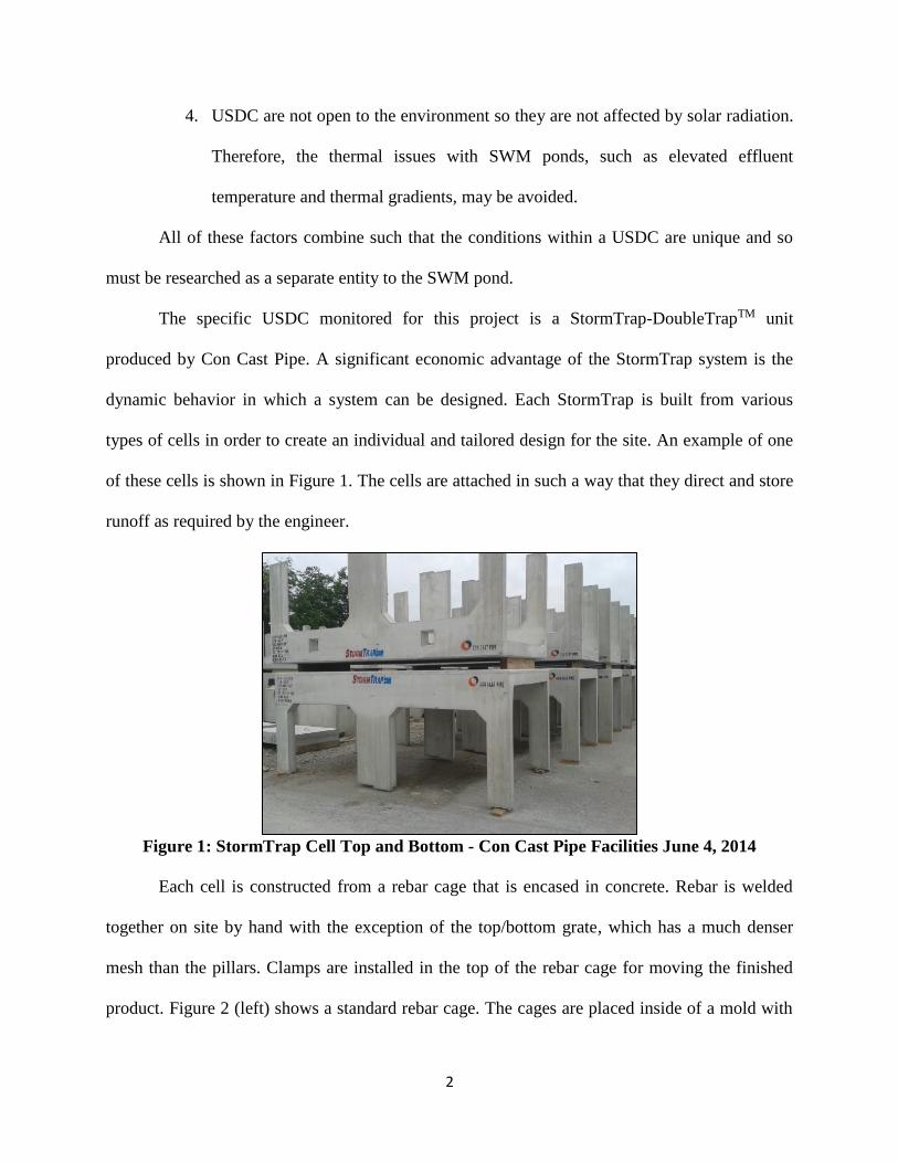
The specific USDC monitored for this project is a StormTrap-DoubleTrapTM unit
produced by Con Cast Pipe. A significant economic advantage of the StormTrap system is the
dynamic behavior in which a system can be designed. Each StormTrap is built from various
types of cells in order to create an individual and tailored design for the site. An example of one
of these cells is shown in Figure 1. The cells are attached in such a way that they direct and store
runoff as required by the engineer.
Figure 1: StormTrap Cell Top and Bottom - Con Cast Pipe Facilities June 4, 2014
Each cell is constructed from a rebar cage that is encased in concrete. Rebar is welded
together on site by hand with the exception of the top/bottom grate, which has a much denser
mesh than the pillars. Clamps are installed in the top of the rebar cage for moving the finished
product. Figure 2 (left) shows a standard rebar cage. The cages are placed inside of a mold with

3
sides that open and close to allow placement of the cage and removal of the finished cell half
(Figure 2 (right)). The molds are coated in a form release agent so that the finished cell can be
removed easily after curing.
Figure 2: StormTrap Rebar Cage (Left), Cell Mold (right) - Con Cast Pipe Facilities June
4, 2014
After the rebar cages are installed, the doors are closed and a high slump concrete is
discharged into the mold. The high slump allows for the concrete to spread easily in and around
the rebar cage and results in a smooth finish for an aesthetic appearance. Manholes can be
installed in the top of a cell by placing a Styrofoam cylinder on top of the rebar cage then
pouring concrete around it. After the concrete has cured, the Styrofoam is removed and a
manhole is placed into the hole that is left. Before and after photos of the concrete pouring
process can be seen in Figure 3 and Figure 4 (left). Following the pouring process, the mold is
covered by a tarp; this tarp holds in steam that is pumped in (Figure 4 (right)). The steam keeps
the concrete moist and regulates the temperature inside the tarp to assist the curing process which
takes 12 hours.

4
Figure 3: StormTrap Cell in Mold (left) with Manhole Styrofoam (right) - Con Cast Pipe
Facilities June 4, 2014
Figure 4: StormTrap after Concrete Pouring (left) Mold Covered by a Tarp (right) - Con
Cast Pipe Facilities June 4, 2014
USDC are an appealing design option for municipalities considering stormwater
management plans because the land on which the system resides can be restored to be used for
alternative purposes, such as parkland, and there is no risk of pedestrians falling in to open water
as with SWM ponds. However, with the strict water quality laws in place for stormwater runoff
treatment, it is risky for engineering consultants to include a newer and less studied technology
in stormwater management designs. A general estimate of cost for a StormTrap is approximately
$250/ m3 for the material and freight, and $50/ m3 for the installation with 500 mm of cover
(Gross, 2015). With more research and design tools available, USDC can be better compared
against other stormwater management technologies and used with greater confidence.

5
The purpose of this research is to gain an understanding of how a USDC acts in an
Ontario climate. Research objectives are to:
1. Identify the stormwater treatment capabilities of underground stormwater
detention chambers using on-site monitoring.
2. Compare the runoff treatment from underground stormwater detention chambers
to stormwater management ponds.
3. Create a model that predicts the removal of contaminants in underground
stormwater detention chambers.
The thesis consists of six chapters, they are structured as follows:
Chapter 1 (Introduction): Introduces thesis topic, outlines objectives, and presents the thesis
structure.
Chapter 2 (Relevant Literature): Presents relative background theory on the removal of
pollutants in SWM ponds and techniques used for modeling this removal.
Chapter 3 (Methodology): Outlines the characteristics of the monitoring site, the equipment
used for monitoring, and how the model was constructed.
Chapter 4 (Water Quality Results): Discusses the results of the site runoff analysis and
compares them to standard SWM pond removal capabilities.
Chapter 5 (Model Results): Discusses the calibration and validation of the SWMM model
hydraulics and hydrology, the assessment of the pollutant removal modeling, and the results of
several simulations.
Chapter 6 (Conclusions and Recommendations): Presents conclusions of the thesis research and
discusses future research directions and recommendations.
Appendix A: Presents the layout of the MUDS Interface as of April 2015.
Appendix B: Provides an explanation of the calculation for removal efficiency by MUDS.
Appendix C: Presents hydrograph and depth figures of storms used for validation and
calibration of the SWMM model.

6
Chapter 2 Relevant Literature
2.1 Urbanization and Stormwater Management
Stormwater management is a key issue in the design of urban infrastructure. Sustained
increases in urbanization have resulted in large-scale replacement of pervious land by impervious
surfaces, which reduces infiltration rates and available surface storage (Natarajan and Davis,
2010). Due to these changes, a larger proportion of urban precipitation becomes runoff. Runoff is
removed from the immediate area through storage and conveyance infrastructure where it is
directed to a nearby water body. Examples of pre- and post-urbanization hydrographs that show
the discharge rate from a watershed can be seen in Figure 5. The pre-urbanization hydrograph
has a significantly smaller peak discharge and the total volume of runoff is far less so there is
less risk of flooding the river or catch basin that is accepting flow from the area.
Figure 5: Pre vs. Post-Urbanization Hydrographs
This phenomenon can be explained simply by using a standard engineering equation for
calculating runoff, the Rational Equation:

7
𝑄𝑝 = 𝑐𝑖𝐴 (1)
where Qp is the peak discharge, c is the runoff coefficient, i is the rainfall intensity, and A is the
drainage area. As an area becomes more impervious, the coefficient c approaches 1, which
results in a larger peak discharge. There are several issues associated with an increased peak
discharge which include: increased flow volumes through rivers; increased flow rates in rivers;
increased duration of high volume and flow rate; and increased frequencies of high runoff events
(Shaver et al., 2007). This results in physical damage to waterways and aquatic habitats by
eroding the soil which supports aquatic plants and shapes the watercourse. A loss of aquatic
plants removes the food source for aquatic organisms and erosion expands the flow channel
increasing flow rates which makes flooding downstream more common (Shaver et al., 2007).
Urban floods occur when the peak discharge exceeds the capacity of the natural and municipal
systems. Depending on the severity of the storm there is potential for significant damage to
property, or even loss of life. For example, a storm which occurred in Toronto in 2013 resulted in
$65 million in damage (National Post, 2014). A stormwater management system will inevitably
fail, but the robustness of the design determines how often it fails and how costly each failure is.
Municipal systems are generally designed for 5-10 year return period events.
Increased runoff volumes are not the only threat to waterways; pollutants which are
prominent in urban areas are transported to receiving water bodies during runoff events.
Pollutants are deposited on impervious surfaces through human activities and atmospheric
deposition; during a runoff event, these pollutants are transported from the surface into the runoff
which then flows into the receiving water body. This process is commonly referred to as non-
point source pollution which is defined as, “having loadings which are discontinuous in time,
frequently not concentrated in a single location, and highly responsive to climate conditions,”
8
(Thomson et al., 1997). The specific types, sources, and environmental issues associated with
stormwater pollutants are explored further in Section 2.2.
The necessity for flow and pollutant control resulting from increased stormwater runoff
has led to the creation of several technologies. These include: coalescing plate separators; dry
detention ponds; wet ponds; constructed wetlands; grassed channels; vegetated filter strips;
porous pavement; and bioretention filters. For a complete explanation of how each of these
technologies function and what they are designed for as well as several more technologies, refer
to Greater Vancouver Sewerage and Drainage District (1999).
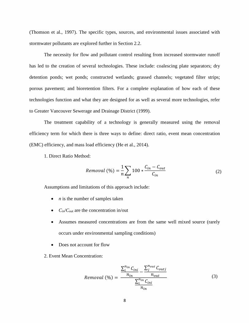
The treatment capability of a technology is generally measured using the removal
efficiency term for which there is three ways to define: direct ratio, event mean concentration
(EMC) efficiency, and mass load efficiency (He et al., 2014).
1. Direct Ratio Method:
𝑅𝑒𝑚𝑜𝑣𝑎𝑙 (%) =
1
𝑛∑ 100 ∗
𝐶𝑖𝑛 − 𝐶𝑜𝑢𝑡
𝐶𝑖𝑛𝑛
(2)
Assumptions and limitations of this approach include:
n is the number of samples taken
Cin/Cout are the concentration in/out
Assumes measured concentrations are from the same well mixed source (rarely
occurs under environmental sampling conditions)
Does not account for flow
2. Event Mean Concentration:
𝑅𝑒𝑚𝑜𝑣𝑎𝑙 (%) =
∑ 𝐶𝑖𝑛𝑖𝑛𝑖𝑛𝑖𝑛𝑖𝑛
−∑ 𝐶𝑜𝑢𝑡𝑗
𝑛𝑜𝑢𝑡𝑗
𝑛𝑜𝑢𝑡
∑ 𝐶𝑖𝑛𝑖𝑛𝑖𝑛𝑖
𝑛𝑖𝑛
(3)

9
Assumptions and limitations of this approach include:
Calculated by averaging the inflow and outflow concentration across the storm
event
Does not account for flow
3. Mass Load Efficiency:
𝑅𝑒𝑚𝑜𝑣𝑎𝑙 (%) =
∑ 𝛥𝑡𝑖 ∗ 𝑄𝑖𝑛𝑖 ∗ 𝐶𝑖𝑛𝑖𝑖 − ∑ 𝛥𝑡𝑗 ∗ 𝑄𝑜𝑢𝑡𝑗 ∗ 𝐶𝑜𝑢𝑡𝑗𝑗
∑ 𝛥𝑡𝑖 ∗ 𝑄𝑖𝑛𝑖 ∗ 𝐶𝑖𝑛𝑖𝑖 (4)
Assumptions and limitations of this approach include:
Conserves total particle mass
Accounts for varying flow
Preferred choice for calculating removal efficiency since it uses conservation of
mass
While these methods are widely used and accepted, there are several issues with the
percent removal efficiency concept. For example, if a treatment technology is tested using a very
polluted sample, then the removal efficiency may be large even if the outlet concentration is still
high. Removal efficiencies do not guarantee that the effluent will not harm aquatic organisms.
Also, even in systems with a short residence time, particle concentrations at the inlet and outlet
may not be closely related (He et al., 2014); particles from previous storm events are present in
the storage and can interfere with the analysis of pollutants from the current storm.
2.2 Stormwater Management Pond Pollutant Characteristics
2.2.1 Total Suspended Solids Total suspended solids (TSS) is a crucial characteristic of runoff. It encompasses not
only clay, sand, and gravel particles which are washed away during runoff events, but also the

10
particulate forms of nutrients, heavy metals, and organics. Sources of TSS in runoff include
construction activities, road sanding/salting, decaying organic matter, metallic dust from car
brakes or engines, and erosion (International Stormwater BMP Database, 2011a). The amount of
TSS which may be present during a runoff event depends on the land use characteristics. The
National Stormwater Quality Database (NSQD) studied this phenomenon and the results can be
seen in Figure 6 (International Stormwater BMP Database, 2011a).
Figure 6: Median Stormwater TSS Concentrations from NSQD
Due to the strong correlation between TSS and other pollutant concentrations, it is
frequently used as an indicator parameter to characterize overall water quality. The broad range
of pollutants which are part of TSS make it strongly correlated with: biochemical oxygen
demand (BOD) - the amount of dissolved oxygen required by organic organisms and increases as
more nutrients are available for reproduction; chemical oxygen demand (COD) – the amount of
dissolved oxygen consumed by contaminants which cannot be oxidized biologically; and heavy
metals such as lead, zinc and copper (Martino et al. 2011). Excessive sediment can adversely
impact aquatic life, source waters for drinking water supply, and water bodies used for

11
recreational activities. The negative effects of excess nutrients and metals are described in
sections 2.2.2 and 2.2.3 respectively.
In stormwater detention systems, suspended solids are removed solely by providing time
for particles to settle (Nix et al., 1988; Jayanti and Narayanan 2004). A detention system is
designed such that particles with a settling velocity greater than the terminal settling velocity –
the settling velocity of the smallest diameter particle which is 100% removed for a given design
event - are removed (Jayanti and Narayanan, 2004). The Ontario Ministry of Environment and
Climate Change (MOECC) defines enhanced protection by a stormwater treatment facility as
having achieved a long-term average removal of 80% suspended solids and by maintaining
maximum flow rates below or equal to pre-development values for storms with design return
periods ranging from 2 to 100 years (Ontario Ministry of Environment, 2003). To obtain the 80%
removal criteria, a sufficient volume must be provided so that, for the given design flow rate, the
particulates have time to settle before exiting the system. The ideal design of a detention facility
is long and thin; this prevents any potential short circuiting by pollutants to ensure that runoff is
treated for the designed length of time. Short circuiting can occur in detention facilities that are
too wide which results in poorer than expected performance. Baffling (Figure 7) is also installed
in cases where a high length to width ratio can not be obtained.

12
Figure 7: Structure With/Without Baffling
Standard TSS removal rates by SWM ponds can be found in Table 1 below. Included in
the table are several sources such as the International Stormwater BMP Database (2011a) and
Shaver et al. (2007) which have summarized data from numerous studies across the United
States of America. Overall, SWM ponds are a reliable way to achieve significant TSS removal in
ranges that achieve enhanced protection under MOECC standards; however, they must be
properly designed and maintained.
Table 1: TSS Removal Percentage by SWM
Source TSS % Removal
International Stormwater BMP Database, 2011a 80
Shaver et al., 2007 50-90
Greater Vancouver Sewerage and Drainage District, 1999 77
House et al., 1993 88
Stormwater Assessment Monitoring and Performance Program, 2005 81-92
Wu et al.,1996 62-93
Pitt, 2003 70-90
2.2.2 Nutrients When designing for stormwater treatment systems, nutrients (nitrogen and phosphorus)
must be adequately removed to maintain a healthy aquatic environment. While these are

13
generated in natural environments and are necessary for the health and growth of aquatic
organisms, excessive loadings of nitrogen and phosphorus from urban stormwater runoff can
have serious repercussions. With an increased concentration of nutrients, there is a greater
potential for eutrophication of the receiving water body. This process results in the rapid
production and decay of organic matter and ultimately in anaerobic conditions and the mass
mortality of organisms (Hu, 2001). Furthermore, as eutrophication progresses there is potential
for aquatic species imbalances, public health threats, and a decline in resource value. As of 2010
over 14,000 water bodies across the United States of America were listed as impaired for
nutrients, organic enrichment, algal growth, and/or ammonia (International Stormwater BMP
Database, 2010).
The effects of eutrophication on ecosystems are not limited to small lakes and rivers but
can even have a significant effect on the Great Lakes. In 2011, Lake Erie experienced its largest
algal bloom in history due to problems with phosphorus enrichment from rural and urban
sources; this resulted in impaired water quality, and impacts on ecosystem health, drinking water
supplies, fisheries, recreation, tourism, and property values (International Joint Commission,
2013). Similar issues as those in Lake Erie have also been found in Lake Simcoe, Ontario
(Environment Canada, 2014). Both urban and rural activities have contributed to the increase of
nutrients in rivers and lakes, some examples include: agriculture, fertilization of lawns and fields,
treated sewage effluent, septic systems, combined sewer overflows, sediment erosion, and
animal waste.
Total phosphorus (TP) and total nitrogen (TN) are present as both soluble and dissolved
forms in stormwater runoff; these phases of nutrients can be further divided. Particulate phase
phosphorus is composed of bacteria, algae, detritus, zooplankton and inorganic particulates such
14
as silt and clay (Shaver et al., 2007). Dissolved phosphorus can be divided into soluble reactive
phosphorus (SRP) and soluble unreactive phosphorus (SUP). SRP is comprised of
orthophosphates and is available for uptake by plants, algae, and microorganisms whereas SUP
is primarily comprised of polyphosphates and various organic compounds not available for
uptake (Shaver et al., 2007). Nitrogen found in stormwater runoff is comprised of nitrate, nitrite,
and total kjeldahl nitrogen (TKN) which is the sum of ammonia, organic, and reduced nitrogen
(United States Environmental Protection Agency, 2015). Vaze and Chiew (2004) found that 85%
of TP and TN are attached particles less than 300µm in diameter. Vaze and Chiew (2004) also
observed that 60% of TP are attached to particles ranging between 11 and 150 µm in diameter;
the majority of TN was also in this range of particles but the fraction was much more variable.
Therefore, by removing suspended particles with diameters of 300 µm and smaller from
stormwater, it will simultaneously proveide water quality treatment for TSS and nutrients. The
dissolved component for TN and TP in urban runoff can range from 20-50% and 20-30%
respectively, this fraction of nutrients is not affected by sedimentation processes (Vaze & Chiew,
2004).
A 2003 study by the Water Environment Research Federation (WERF) found that by
removing TP and phosphate particles with diameters greater than 20, 5, and 0.45µm,
approximately 70, 80, and 90% of the particles were removed, respectively. Median
concentrations of total and soluble phosphorus, ammonia, and nitrate and nitrite based on land
use were found by the NSQD and the National Urban Runoff Program (NURP); these can be
seen in Table 2 below (International Stormwater BMP Database, 2010).

15
Table 2: Median Total and Soluble Phosphorus, Ammonia and Nitrate/Nitrite
Concentrations by Land Use
Source Residential Mixed Commerical Open Space/Non-Urban
NSQD
TP (mg/L) 0.17 - 0.11 0.13
Ammonia (mg/L 0.32 - 0.50 0.18
Nitrate and Nitrite (mg/L) 0.60 - 0.60 0.59
NURP
TP (mg/L) 0.38 0.26 0.20 0.12
Soluble P (mg/L) 0.14 0.056 0.08 0.026
The removal and transformation mechanisms for the various forms of nitrogen and
phosphorus have been summarized in Table 3 and were adapted from the International
Stormwater BMP Database (2010).
Table 3: Summary of Nitrogen and Phosphorus Transformations and Removal
Mechanisms
Species Transformation and Removal Mechanisms
Particulate Phosphorus Physical separation (filtration and sedimentation)
Orthophosphates Adsorption/precipitation onto soil
Plant and microbial uptake
Nitrogenous Organic
Solids
Physical separation (filtration and sedimentation)
Ammonification (transform via microbial decomposition to NH4
Nitrate (NO3)
Plant uptake
Denitrification (removal via biological reduction to N2 gas and
volatilization)
Ammonia (NH4+, NH3)
Volatilization
Nitrification (transform via biological oxidation to NO3 via NO2)
The MOECC developed general guidelines for concentrations of ammonia and total
phosphorus (TP) to prevent aesthetic and water quality deterioration. For un-ionized ammonia, a
guideline of 20µg/L was set (Ministry of Environment and Energy, 1994). For TP, the guidelines
recommended are 10µg/L for a high level of protection against aesthetic deterioration, 20µg/L to
avoid nuisance concentrations of algae in lakes, and 30µg/L to prevent excessive plant growth in
rivers and streams (Ministry of Environment and Energy, 1994).

16
Removal efficiency of SWM ponds for nutrients in stormwater runoff are shown in Table
4. There is a wide range in removal efficiency. This is most likely due to variations in local
conditions such as vegetation type and quantity, and the dissolved fraction of nutrients.
Table 4: Nutrient Removal Efficiency by SWM Ponds
Source TN TKN
Nitrite +
Nitrate Nitrate TP
TSP
(Soluble) DP
Ortho-
PO4
International
Stormwater BMP
Database, 2010
27 15 62
59
45 64
Shaver et al., 2007 30
50
Greater Vancouver
Sewerage and
Drainage District,
1999
30
24 47 51
House et al., 1993
38 65
38
Stormwater
Assessment
Monitoring and
Performance Program,
2005
42-87
Wu et al., 1996
21-32
36-45
Pitt, 2003 60-70
60-70
2.2.3 Heavy Metals In urban environments, heavy metals originate primarily from automobiles and exposure
of building materials to rain; if a metal is naturally abundant then it may be present in stormwater
due to soil erosion and weathering. Treated wood, tires, and atmospheric deposition are also
common sources of metals (International Stormwater BMP Database, 2011b). A summary of the
sources of several common metals are shown in Table 5. Metal concentrations in stormwater
runoff have been found to be 10-100 times the average concentration in sanitary effluent water
(Sansalone and Cristina, 2004). As of 2011, over 7,400 water bodies in the United States of
America are listed as impaired due to metals (USEPA, 2015).

17
Table 5: Common Sources of Metal in Urban Runoff (Shaver et al., 2007)
Metal Source
Copper
Building materials
Paints and wood preservatives
Algaecides
Brake pads
Zinc
Galvanized metals
Paints and wood preservatives
Roofing and gutters
Tires
Lead
Gasoline
Paint
Batteries
Chromium Electro-plating
Paints and preservatives
Cadmium Electro-plating
Paints and preservatives
Heavy metals have been associated with many illnesses in humans and have strict
concentration guidelines in wastewater and drinking water treatment. However, there are no
MOECC requirements for treatment of heavy metals in stormwater runoff. While this water is
treated prior to distribution in drinking water systems to prevent human illness, it still poses a
risk to aquatic ecosystems as the metals can bioaccumulate in organisms, which has adverse
effects (Center for Hazardous Substance Research, 2009). Typical levels of metals that are found
in stormwater runoff can be seen in Table 6 which was adapted from Shaver et al. (2007).
Table 6: Typical Levels of Metals Found in Stormwater Runoff (µg/L)
Metal Stormwater Median
(90th Percentile)a
Mean
(sd)b
Median (Cov)
Urban
Stormwaterc
Range for
Highway
Runoffd
Range for
Parking lot
Runoffe
Arsenic N/A 5.9 (2.8) 3.3 (2.42) 0-58 N/A
Cadmium N/A 1.1 (0.7) 1.0 (4.42) 0-40 0.5-3.3
Chromium N/A 7.2 (2.8) 7.0 (1.47) 0-40 1.9-10
Copper 34 (93) 33 (19) 16.0 (2.24) 22-7033 8.9-78
Lead 144 (350) 70 (48) 15.9 (1.89) 73-1780 10-59
Mercury N/A N/A 0.2 (1.17) 0-0.322 N/A
Nickel N/A 10 (2.8) 9.0 (2.08) 0-53.3 2.1-18
Silver N/A N/A 3.0 (4.63) N/A N/A
Zinc 160 (500) 215 (141) 112.0 (4.59) 56-929 51-960
Sources of Research Cited by Shaver et al. 2007: aUSEPA, 1983. bSchiff et al., 2001. cPitt et al., 2002. dBarrett et al., 1998. eTiefenthaler et al., 2001
18
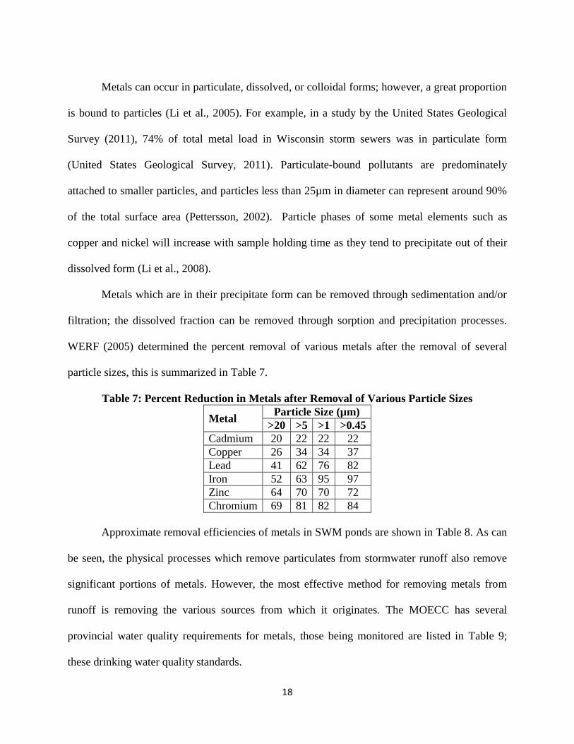
Metals can occur in particulate, dissolved, or colloidal forms; however, a great proportion
is bound to particles (Li et al., 2005). For example, in a study by the United States Geological
Survey (2011), 74% of total metal load in Wisconsin storm sewers was in particulate form
(United States Geological Survey, 2011). Particulate-bound pollutants are predominately
attached to smaller particles, and particles less than 25µm in diameter can represent around 90%
of the total surface area (Pettersson, 2002). Particle phases of some metal elements such as
copper and nickel will increase with sample holding time as they tend to precipitate out of their
dissolved form (Li et al., 2008).
Metals which are in their precipitate form can be removed through sedimentation and/or
filtration; the dissolved fraction can be removed through sorption and precipitation processes.
WERF (2005) determined the percent removal of various metals after the removal of several
particle sizes, this is summarized in Table 7.
Table 7: Percent Reduction in Metals after Removal of Various Particle Sizes
Metal Particle Size (µm)
>20 >5 >1 >0.45
Cadmium 20 22 22 22
Copper 26 34 34 37
Lead 41 62 76 82
Iron 52 63 95 97
Zinc 64 70 70 72
Chromium 69 81 82 84
Approximate removal efficiencies of metals in SWM ponds are shown in Table 8. As can
be seen, the physical processes which remove particulates from stormwater runoff also remove
significant portions of metals. However, the most effective method for removing metals from
runoff is removing the various sources from which it originates. The MOECC has several
provincial water quality requirements for metals, those being monitored are listed in Table 9;
these drinking water quality standards.

19
Table 8: Percent Removal of Metals by SWM
Source Total
Arsenic
Total
Cadmium
Total
Chromium
Total
Copper
Total
Iron
Total
Lead
Total
Nickel
Total
Zinc
International
Stormwater
BMP Database,
2011b
23 33 60 40 76 70 53 62
Greater
Vancouver
Sewerage and
Drainage
District, 1999
24
57
73
51
Stormwater
Assessment
Monitoring and
Performance
Program, 2005
10-67
70-87
Wu et al., 1996
52-87
32-80
Table 9: Metals Provincial Water Quality Requirements
Metal Provincial Water Quality Requirement (μg/L) Aluminum *(Interim) 75 Antimony *(Interim) 20
Arsenic 100 Barium N/A
Beryllium Hardness < 75 mg/L - 11 Hardness > 75 mg/L - 1100
Boron 200
Cadmium *(Interim) Hardness 0-100 mg/L - 0.1 Hardness > 100 mg/L - 0.5
Chromium 1 hexavalent, 8.9 trivalent Cobalt 0.9 Copper 5
Iron 300
Lead *(Interim) Hardness < 30 mg/L - 1
Hardness 30-80 mg/L - 3 Hardness > 80 mg/L - 5
Manganese N/A Molybdenum *(Interim) 40
Nickel 25 Selenium 100
Silver 0.1 Strontium N/A
Thallium *(Interim) 0.3 Titanium N/A
Uranium *(Interim) 5 Vanadium *(Interim) 6
Zinc *(Interim) 20

20
2.2.4 Temperature The thermal properties of an aquatic system are generally determined by local
environmental and weather conditions, such as heat from the overlying air, solar radiation, and
heated urban runoff (Song et al., 2013). SWM ponds consistently produce thermally enriched
effluent due to prolonged exposure to solar radiation during detention and runoff that underwent
heat exchange with impervious surfaces. As the effluent enters a receiving water body it can
cause damage to local ecosystems. For example, increases in stream temperature can negatively
impact behaviour, metabolism, reproduction, growth, and vulnerability to disease in various
Trout species (Jones, 2008).
Thermal stratification – when a relationship exists between the depth and temperature of
water – has been observed in SWM ponds (Jones, 2008). This is due to extended detention times
and solar radiation heating the surface of the pond. Strong stratification can slow or prevent the
exchange of materials between the surface and bottom waters. Song et al. (2013) studied thermal
stratification patterns in urban ponds and found that concentrations of dissolved oxygen were
consistently higher in the surface relative to bottom waters and higher concentrations of
suspended solids, TP, and particulate nutrients were in bottom waters. Differences in TP and
particulate phosphorus were strongly related to stratification intensity, but differences in total
dissolved phosphorus concentrations were significantly related to the duration of stratification
rather than intensity. If thermal stratification occurs in a USDC, it may act similarly to SWM
ponds.
USDC are a potential mitigation to elevated runoff temperatures. Natarajan and Davis
(2010) studied a USDC in Maryland and showed that its outflow temperatures were more
uniform compared to the runoff. The USDC achieved a mean reduction in temperature of 1.6oC
during July, and its mean outflow temperature was only 19.7oC. This reduction in temperature

21
was attributed to the cooler ambient air temperatures in a USDC and the lack of solar radiation.
Accordingly, the USDC did not have a cooling effect on runoff at lower temperatures. The
thermal effects of USDC was not reported.
2.2.5 First Flush The first flush of contaminants from the beginning of a storm event delivers a high
concentration or mass of pollutants into the receiving water body (Sansalone and Cristina, 2004).
In some cases, the stormwater runoff pollution in first flush can be comparable to or greater than
sewage pollution (Martino et al., 2011). Although the potential for occurrence of first flush is
widely recognized there is no unified definition but many have been proposed (Hallberg, 2006).
For example, Bertrand-Krajewski et al. (1998) propose a 30/80 first flush definition where 80%
of the pollutants from a runoff event occur in the first 30% of flow into a facility; but 20/80 and
25/50 definitions have also been proposed by Stahre and Urbonas (1990) and Wanielista and
Yousef (1993) respectively. Designing for, or enhancing, the treatment of first flush runoff can
improve the overall performance of a treatment facility (Li et al., 2008).
There are two ways of determining whether a first flush has occurred; mass-based and
concentration-based methods (Sansalone and Cristina, 2004). The mass-based method is defined
by the following formula:
Cumulative Mass (t)
Total Mass>
Cumulative Volume (t)
Total Volume (5)
This method is particularly appealing as it can be interpreted graphically with ease, using
a mass-volume (M(V)) curve, and it can be used to compare storms on a similar scale regardless
of storm length (Figure 8). M(V) curves have been shown to fit well with the following formula:
𝑌 = 𝑋𝑏 (6)

22
where Y is the Cumulative Mass/Total Mass and X is the Cumulative Volume/Total Volume
(Bertrand-Krajewski et al., 1998). Higher values of b indicate a higher first flush effect
(Sansalone and Cristina, 2004).
Figure 8: 25/50 M(V) Curve
The concentration based method is not so mathematically straightforward, but is instead a
set of conditions which suggest a first flush has occurred. First, there must be a high initial
concentration followed by a rapid concentration decline. Subsequently, there is a relatively low
and constant concentration.
2.2.6 Winter Conditions
During the winter, pollutant load increases dramatically; this is due to the use of de-icing
agents which increase the chloride and TDS concentrations (Hallberg, 2006, Marsalek et al.,
2003). Studded tires which are used during the winter also contribute to larger TDS
concentrations as they increase the wear on asphalt pavement (Hallberg, 2006).
Marsalek et al. (2003) noted several characteristics in SWM ponds that occur through the
winter. The ice layer which seperates the pond water from the air caused the water to lag air
0
0.1
0.2
0.3
0.4
0.5
0.6
0.7
0.8
0.9
1
0 0.2 0.4 0.6 0.8 1
Y:
Cu
mu
lati
ve M
ass/
To
tal M
ass
X: Cumulative Volume/ Total Volume

23
temperature by 3-4 days, the amplitude for water temperature was 4.4oC less than air
temperature, and fluctuations in daily water temperature were 1/3 that of the air temperature.
Marsalek et al. also observed that the dissolved oxygen (DO) concentration decreased to 0 from
mid-December to mid-January, this is undesireable because a lack of DO can lead to the
mortality of aquatic organisms and plants. Lastly, density stratification occurred due to thermal
stratification and chemical stratification by dissolved solids (particularly chloride) (Marsalek et
al., 2003).
2.3 Modeling of Stormwater Management Ponds
SWM and the USDC use similar removal processes to treat pollutants in stormwater
runoff. Therefore, many of the models that have been developed for SWM ponds and
sedimentation tanks can be applied or modified to simulate the removal of pollutants in USDC.
2.3.1 K-C Decay Rate Model The K-C model has been shown to be applicable for vegetated and non-vegetated ponds
(Wong et al., 2006). Reactor kinetics which are prominent in water and wasterwater treatment
processes are used to create the decay rate formula (Equation 7).
𝑟𝐴 =
𝑑𝐶
𝑑𝑡= −𝑘𝐶𝐴
𝑛
(7)
The reaction rate (rA) is defined as the change in concentration of the pollutant over time
(mg/L∙s), k is a decay rate constant which is specific to the pollutant, and CA is the concentration
of the pollutant in the SWM pond (mg/L). The value of n defines the order of the reaction (eg.
first order, second order) with higher orders decaying at faster rates.
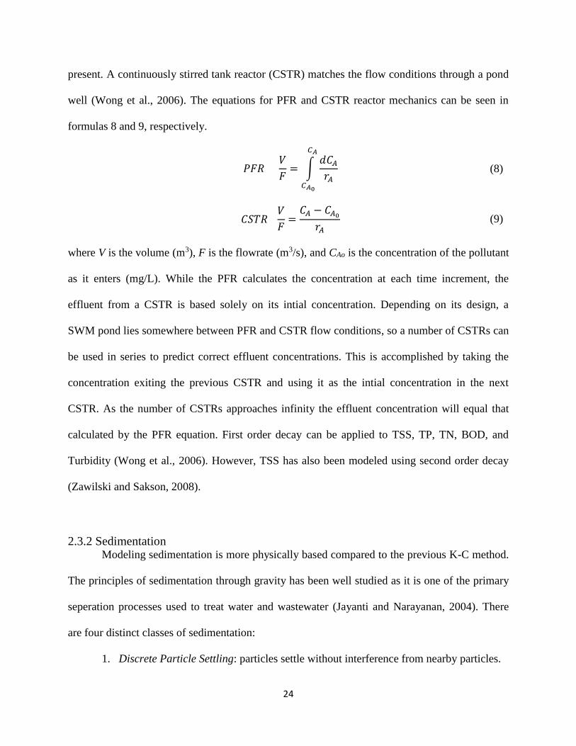
Conceptually, a stormwater pond will follow plug-flow reactor (PFR) mechanics.
However this condition rarely, if ever, occurs in the field as some degree of mixing is always
24
present. A continuously stirred tank reactor (CSTR) matches the flow conditions through a pond
well (Wong et al., 2006). The equations for PFR and CSTR reactor mechanics can be seen in
formulas 8 and 9, respectively.
𝑃𝐹𝑅 𝑉
𝐹= ∫
𝑑𝐶𝐴
𝑟𝐴
𝐶𝐴
𝐶𝐴0
(8)
𝐶𝑆𝑇𝑅
𝑉
𝐹=
𝐶𝐴 − 𝐶𝐴0
𝑟𝐴 (9)
where V is the volume (m3), F is the flowrate (m3/s), and CAo is the concentration of the pollutant
as it enters (mg/L). While the PFR calculates the concentration at each time increment, the
effluent from a CSTR is based solely on its intial concentration. Depending on its design, a
SWM pond lies somewhere between PFR and CSTR flow conditions, so a number of CSTRs can
be used in series to predict correct effluent concentrations. This is accomplished by taking the
concentration exiting the previous CSTR and using it as the intial concentration in the next
CSTR. As the number of CSTRs approaches infinity the effluent concentration will equal that
calculated by the PFR equation. First order decay can be applied to TSS, TP, TN, BOD, and
Turbidity (Wong et al., 2006). However, TSS has also been modeled using second order decay
(Zawilski and Sakson, 2008).
2.3.2 Sedimentation Modeling sedimentation is more physically based compared to the previous K-C method.
The principles of sedimentation through gravity has been well studied as it is one of the primary
seperation processes used to treat water and wastewater (Jayanti and Narayanan, 2004). There
are four distinct classes of sedimentation:
1. Discrete Particle Settling: particles settle without interference from nearby particles.

25
2. Flocculent Settling: particles collide and adhere to one another increasing the settling
velocity
3. Hindered (or Zone) Settling: particles settle as a extremely high concentration layer
which has a single settling velocity
4. Compression Settling: particles that have settled to the bottom are compressed by
gravity.
In SWM ponds, sedimentation can be modeled using discrete particle settling, as no
flocculating agents are added to induce flocculent or hindered settling, and compression settling
has no effect on the effluent pollutant concentration. Fine suspended particles can flocculate of
their own accord, but will break up under certain flow conditions (Krishnappan & Marsalek,
2002); so, it is not a mechanism that can be reliably modeled and may overpredict removal
efficiency.
The removal efficiency is determined by ascertaining the critical settling velocity, which
is the flow rate divided by the SWM pond surface area. All particles with diameters larger than
the particle with a settling velocity equal to the critical settling velocity are fully removed. Some
of the smaller particles will settle while others flow out of the system; this depends on their
elevation after they enter the SWM pond and have been subject to turbulent mixing. The fraction
which is removed is directly proportional to their settling velocity divided by the critical settling
velocity. Figure 9 shows the potential paths a particle can take in a settling tank. V1 represents
the path of a particle with the terminal settling velocity, V2 has a settling velocity greater than
V1, and V3 has a settling velocity less than V1. If V3 entered at a higher elevation then the
particle would have exited the system.

26
Figure 9: Particle Sedimentation Paths
Stokes’ law (Equation 10) is commonly used to describe the settling velocity of a discrete
spherical particle for a given diameter and particle density:
𝑉𝑠 =
1
18
𝜌𝑠 − 𝜌𝑤
µ 𝑔𝑑𝑝
2
(10)
where ρs is the particle density (kg/m3), ρw is the water density (kg/m3), µ is the dynamic
viscosity of the fluid (Pa∙s), g is the gravitational constant (m/s2), and dp is the diameter of the
particle (m).
There are several assumptions in Stokes’ Law which may affect the accuracy. Firstly, the
velocity is heavily dependent on the density of the particle and this has an effect on the removal
efficiency; the lower the density, the lower the removal efficiency (Takamatsu et al., 2006). The
specific gravity of most soils and rocks typical in runoff is 2.65 (Freeze and Cherry, 1979).
However, Karamalegos (2006) reported that particles with diameters less than 75 µm had
average densities ranging from 0.81 g/cm3 to 2.80 g/cm3. Due to the variability in density,
Stokes’ law may over predict the removal efficiency of a sedimentation tank. The density of
particles has a significant effect on removal efficiency especially below 2 g/cm3 (Takamatsu et
al., 2010). Secondly, there is high variability in particle size distributions between and within a
site as well as over time. Variability between samples collected from a single site can often be
greater than the variability between samples collected from different sites (Toronto and Region
Conservation Authority, 2012a). Therefore, accurately and consistently predicting sedimentation

27
on a storm-by-storm basis is challenging. In Ontario, the Toronto and Region Conservation
Authority (2012a) have found that SWM pond samples collected throughout the Greater Toronto
Area often have finer particle size distributions than those collected in many other cold climate
jurisdictions. Lastly, the shape of the particles are unlikely to be spherical which is a basic
assumption of Stokes’ Law. Particle shape can range so any random particle may fall slower or
faster than a perfect sphere; therefore, this assumption is least likely to have a significant effect
on average settling velocity prediction.
Takamatsu et al. (2010) produced a sedimentation model which uses Stokes’ Law in
combination with the hydraulics of a dry stormwater pond (no permanent pool). This “pathline”
model tracks the location in the x and y direction of particles of a given diameter through a storm
event. Takamatsu et al. (2010)'s model consistently underestimated the removal efficiency of the
dry pond but only by a few percent.
2.3.3 Probabilistic Many runoff event properties can be described using probability distributions due to their
stochastic nature. The EMC of various pollutants are often described using a log-normal
distribution (Strecker et al., 2001, Buren et al., 1997, German and Svensson, 2002). However,
effluent concentrations have also been shown to follow normal distributions (Buren et al., 1997).
Table 10, which was adapted from Buren et al. (1997), shows the distributions associated with
various pollutants. EMC have been correlated with pollutant concentration in pond sediment
(German and Svensson, 2002). Particle size distributions in runoff and settling velocities for a
specific particle diameter can alse be described by log-normal distributions (Takamatsu et al.,
2006, Li et al.,2008).

28
Adams and Papa (2000), and Loganathan et al. (1985) have produced probabilistic
models to describe hydraulic and hydrologic processes of stormwater retention and detention
systems. These models provide a range of possibilities that a system may experience but cannot
predict results on a storm-by-storm basis.
Table 10: Distribution of Event Constituents (EMC)
Pollutant Source
Parking lot Creek inflow Pond Outflow
Constituent PL W2 PL W2 PL W2
TSS
TDS
COD
Chloride
TP
Sol. P
Sulphate
Ammonia
Sol. TKN -
Tot. TKN -
Oil & Gr
Phenol - -
-
Copper - -
-
Zinc - -
-
Normal PL – Results interpreted from a probability plot
Log-Normal
W2- Results from 95% acceptance Cramer-Von
Mises tests
Either
Neither -
2.4 Summary
The chapter above explains the necessity for controlling and treating runoff in an urban
environment. Preventing damage to receiving water bodies through high flow rates, high runoff
volumes, and the subsequent release of pollutants is essential to prevent damage to aquatic
environments. Furthermore, stormwater management systems assist in the prevention of

29
flooding, erosion, and damage to source waters which can have negative effects on health, safety,
and the local economy (Shaver et al., 2007).
The chapter describes common pollutants found in urban runoff including their sources
and the effectiveness of treatment by SWM ponds. TSS is an important factor for ensuring a
stormwater management system has been properly designed, it is often used as an indicator
parameter to assess overall water quality and compare removal processes. In Ontario, SWM
ponds are often designed with the intention of removing 80% of TSS which is the standard for
enhanced protection under MOECC standards (Ontario Ministry of Environment, 2003). Other
water quality characteristics that are commonly studied include the concentrations of nutrients,
metals, and temperature at the inlet and outlet of stormwater management systems; excessive
levels of any of these pollutants can cause severe damage to aquatic environments (International
Joint Commission, 2013).
The chapter also summarizes the common methods for modeling the removal of
pollutants by SWM ponds and settling tanks including the direct ratio method, event mean
concentrations, and mass load efficiencies. Removal of suspended sediments in a SWM pond can
be simulated using K-C decay models, sedimentation, or probabilistic models. Modeling the
process of sedimentation through physically based data is a straightforward and accurate method.
The literature presented in this chapter are applied in the following chapters to determine
the hydraulic and water treatment performance of the Markham UDSC. Conceptual and
theoretical models presented from this chapter are applied in the methodology discussed in
Chapter 3 to develop, test and apply MUDS using water quality data collected from the
Markham USDC

30
Chapter 3 Methodology
3.1 Field Site
The specific USDC monitored for this project services the South Unionville Square
development in the City of Markham, Ontario (Figure 10). The drainage area serviced by the
DoubleTrapTM is a new 5.24 hectare commercial and residential mixed-use development and is
one of the first in Ontario to feature such a system (Toronto and Region Conservation Authority,
2012b). The DoubleTrapTM was installed in July 2010 but was not connected to its full drainage
area until late 2011. One small section located immediately south of the DoubleTrapTM, across
South Unionville Avenue, remained under construction during this study. Sediment wash-off
from the construction site into the DoubleTrapTM was not a concern because little to no runoff
was expected because there was abundant surface storage in this area. Additionally, the site
occupied only a small portion of the total catchment area (6%).
Originally, a SWM pond was planned to control runoff, but was replaced with a
DoubleTrapTM in 2010 in order to double the available parkland. The DoubleTrapTM receives
runoff from the catchment and wastewater from a splash pad in the park. Several boxes which
contain monitoring equipment and prevent the public from accessing the system’s hatches are the
only indications that a USDC is installed on the site. Additional photos of the park, surrounding
area, and the remaining construction zone are shown in Figure 11 and Figure 12.

31
Figure 10: DoubleTrapTM Location and Service Area
Figure 11: DoubleTrapTM Site and Monitoring Boxes (Left), Construction Zone South of
the DoubleTrapTM (Right) (June 23, 2014)

32
Figure 12: Parkland Surrounding the DoubleTrapTM (June 23, 2014)
Figure 13 and Figure 14 show the various dimensions of the USDC. The DoubleTrapTM
has an approximate 1,200 m2 footprint, a maximum height of 3.4 m, and side lengths of 51.5 m
and 23.1 m. A permanent pool of 1,475 m3 is provided for water treatment, and an extended
storage volume of 1,143 m3 allows for a 25 mm storm to drain over 24 hours. A 1,200 mm pipe
at a height of 1.39 m relative to the bottom of the USDC directs runoff from the stormwater
sewer into the system. A 120 mm orifice plate installed in a 300 mm pipe drains water from the
system during a storm event; the maximum design flow rate is 0.03 m3/s which corresponds to
the preconstruction flow for a 5-year return period storm event. Two 525 mm overflow pipes are
installed and have a maximum flow rate of 1.39 m3/s. The 300 mm and 525 mm pipes are
installed at heights of 1.39 m and 2.45 m, respectively, relative to the bottom of the USDC.
Figure 15 shows the USDC as it has been built as well as its individual cells.

33
Figure 13: DoubleTrapTM Monitoring Equipment and Dimensions
Figure 14: DoubleTrapTM Dimensions (Side)
Figure 15: As Built DoubleTrapTM with Individual Cells

34
3.2 Monitoring
Monitoring was conducted by Toronto and Region Conservation Authority (TRCA)
technicians from May 2014 to early December 2014. The monitored water quality parameters
include: TSS, nutrients, metals, oil and grease, chloride, bacteria, turbidity, temperature, DO and
conductivity. The location of the various samplers and monitoring equipment is shown in Figure
13 with an explanation of each sensor in Table 11. Precipitation measurements were taken at
Milne Dam in the City of Markham, which is three kilometers east of the site (Figure 10). Flow-
weighted composite samples were collected and sent for water quality analyses at a MOECC lab.
The Hobo Water Level Logger and YSI monitors were positioned 0.04 m above the bottom of
the USDC. Data from the MOECC lab and monitoring equipment was sent to the University of
Toronto for processing and analysis.
Table 11: DoubleTrapTM Monitoring Equipment Properties and Purpose
Parameter Equipment Frequency Accuracy
Water Quality
ISCO Auto-samplers coupled
with water level sensors to
trigger start and end of
sampling
All storm events that
generate enough flow to
trigger the sampler
Water Level HOBO Water Level Logger Continuous measurements
at 5 minute intervals ± 3 mm
Temperature Hobo Water Level Logger Continuous measurements
at 5 minute intervals
±0.44o
(from 0 o to 50 oC)
Turbidity YSI monitors Continuous measurements
at 5 minute intervals
± 2% of reading or
0.3 NTU, whichever
is greater
Flow Rate/Volume ISCO ultrasonic water level
sensor attachment
Continuous measurements
at 5 minute intervals
± 0.03 m/s
(-1.5 to 1.5 m/s)
±2% of reading (1.5
to 6.1 m/s)
Conductivity/
Temperature
Profiles
Probe lowered to regular depth
intervals
Four profiles conducted
during summer and winter
seasons
Precipitation
0.2 mm Four season (heated)
tipping bucket precipitation
gauge
Continuous measurements
at 5 minute intervals

35
Hydraulic and water quality data collection was scheduled to begin in early May, but was
delayed due to construction and clean out activities. The parkland which houses the Markham
USDC remained under construction throughout May, and the permanent pool of the USDC
contained a significant amount of construction sediment that had eroded and washed off from the
surrounding area. Under these conditions, any data collected would be an inappropriate
representation of the hydraulics and treatment capability of the catchment and USDC. The
excessive sediment loads caused by the construction activities as well as the sediment already
present in the USDC permanent pool generated much higher pollutant concentrations than
typical urban runoff. By May 29th the park was finished, the USDC was emptied and cleaned so
useful data could start being collected.
The cleaning of the USDC required the permanent pool to be emptied. Afterwards, the
permanent pool filled gradually with runoff. Until June 21st, any runoff that occurred would not
generate outflow since the permanent pool needed to be refilled by runoff in the catchment.
Closely following the resumption of outflow, the orifice plate was clogged by garbage. This
interfered with the outflow measurements causing them to vary widely over short periods and not
be easily predicted by hydraulic equations. The orifice plate was unclogged on July 10th allowing
several storms to be monitored successfully until, on July 27th, the orifice plate was clogged
again. This was the final time that clogging occurred during the monitoring period, and was
remedied on August 12th.
In mid-August the Town of Markham installed a splashpad at the park which had an
outlet leading to the inlet of the USDC. On several occasions, the splashpad was observed
flowing during storm events. The inflow hydrograph for the model was generated using SWMM
so it can only account for flows due to rainfall, making accurately predicting the outflow difficult

36
due to the unknown splashpad flow rate. This was also causing issues with sample collection as
the ISCO sampler at the inlet would activate due to the splashpad flow and capture water that
was previously in the municipal water system instead of runoff from the catchment. To account
for these issues, a flowmeter was installed in the piping leading from the splashpad to the USDC
inlet and the sampling tube of the ISCO sampler was moved further up the stormsewer system
where it would not receive flow from the splashpad. The splashpad was shut down on September
17th.
Monitoring continued until December 2nd when the equipment was removed for the
winter. There were no issues gathering hydraulic data until this point. However, the turbidity
meters malfunctioned in November with the YSI monitor near Hatch 1 providing negative values
until November 10th, and the YSI monitor near Hatch 5 providing negative or unreasonably low
values until November 24th. For this reason water quality could not be modeled for the storm
events that occurred in November but could still be used for hydraulic calibration.
During the monitoring phase it was also discovered that the Markham USDC had been
overdesigned. Originally the USDC was supposed to accept runoff from close to 8 hectares but a
section of the catchment area was excluded later, so it only receives runoff from a 5.24 hectare
catchment. Therefore, the USDC should perform above expectations for storms that would cause
a failure to occur for a more optimally designed USDC.
3.3 Water Quality Analysis
Descriptive statistics such as: range, average, median, and standard deviation, were
calculated. Statistical analyses were used to determine whether the average concentration of a
given pollutant changed to a 95% significance level (p<0.05). Paired t-tests were performed to
compare the average EMC of pollutants observed at the inlet, Hatch 2, and outlet. Paired t-tests

37
operate under the assumption that the data is represented by a normal distribution, in order to
ascertain the distribution of data for each pollutant, the EPA's statistical software ProUCL 5.0
was utilized. If the data was not normally distributed it was transformed using conversion
formulae specific to the actual distribution. Paired t-tests were performed with the transformed
data set to determine statistical significance.
3.4 Modeling
This section presents the methodologies used by The Model for Underground Detention
of Sediment (MUDS) to predict TSS removal efficiency of a USDC. The basic mathematical and
physical principles that govern the hydraulics, particle tracking, and pollutant removal are
discussed. A summary of a Storm Water Management Model (SWMM) that was also created to
estimate inflows to the Markham USDC is also included.
MUDS was constructed by Nicholas McIntosh at the University of Toronto in 2014, it
utilizes Excel’s interface combined with the Visual Basic compiler that is accessible through
Excel’s Macro function. MUDS is designed to simulate the hydraulics and pollutant removal of a
USDC regardless of location and layout. The required input parameters are: an inflow
hydrograph; timestep length; USDC dimensions; the particle size distribution (d10 – d90) and
density of pollutants in runoff; water density and dynamic viscosity; and the first flush
pollutant/flow proportion. These parameters are used to calculate the outflow hydrograph and
TSS removal efficiency. The large number of variables makes MUDS versatile for a broad range
of design applications. Runoff inflows to the Markham DoubleTrapTM could not be directly
monitored because the stormwater inlet and outlet are at the same elevation; therefore, the inlet
water levels fluctuate with the active storage inside the Markham USDC which can cause
backwater conditions at the inlet. As a result, inflow hydrographs were generated by creating a
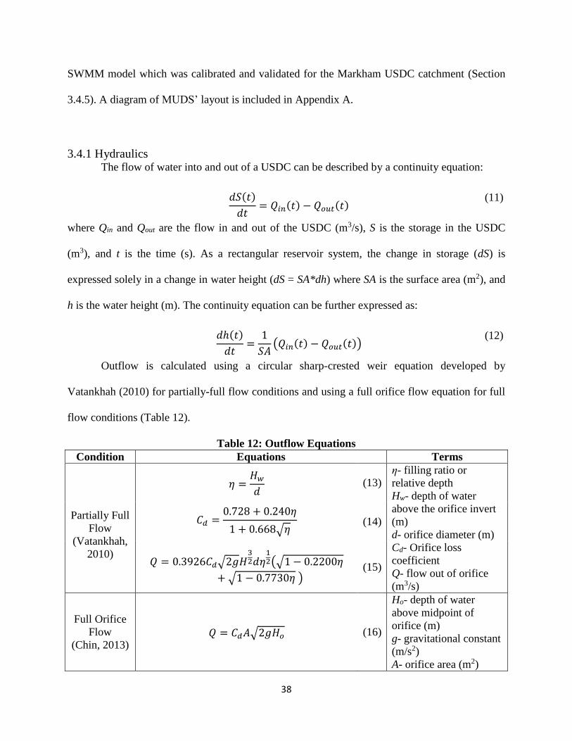
38
SWMM model which was calibrated and validated for the Markham USDC catchment (Section
3.4.5). A diagram of MUDS’ layout is included in Appendix A.
3.4.1 Hydraulics The flow of water into and out of a USDC can be described by a continuity equation:
𝑑𝑆(𝑡)
𝑑𝑡= 𝑄𝑖𝑛(𝑡) − 𝑄𝑜𝑢𝑡(𝑡)
(11)
where Qin and Qout are the flow in and out of the USDC (m3/s), S is the storage in the USDC
(m3), and t is the time (s). As a rectangular reservoir system, the change in storage (dS) is
expressed solely in a change in water height (dS = SA*dh) where SA is the surface area (m2), and
h is the water height (m). The continuity equation can be further expressed as:
𝑑ℎ(𝑡)
𝑑𝑡=
1
𝑆𝐴(𝑄𝑖𝑛(𝑡) − 𝑄𝑜𝑢𝑡(𝑡))
(12)
Outflow is calculated using a circular sharp-crested weir equation developed by
Vatankhah (2010) for partially-full flow conditions and using a full orifice flow equation for full
flow conditions (Table 12).
Table 12: Outflow Equations
Condition Equations Terms
Partially Full
Flow
(Vatankhah,
2010)
𝜂 =𝐻𝑤
𝑑 (13)
η- filling ratio or
relative depth
Hw- depth of water
above the orifice invert
(m)
d- orifice diameter (m)
Cd- Orifice loss
coefficient
Q- flow out of orifice
(m3/s)
𝐶𝑑 =0.728 + 0.240𝜂
1 + 0.668√𝜂 (14)
𝑄 = 0.3926𝐶𝑑√2𝑔𝐻32𝑑𝜂
12(√1 − 0.2200𝜂
+ √1 − 0.7730𝜂 ) (15)
Full Orifice
Flow
(Chin, 2013) 𝑄 = 𝐶𝑑𝐴√2𝑔𝐻𝑜 (16)
Ho- depth of water
above midpoint of
orifice (m)
g- gravitational constant
(m/s2)
A- orifice area (m2)

39
The partially full flow is significantly influenced by the ratio of depth above the orifice
invert to the diameter of the orifice (η). As the depth increases, the loss coefficient (Cd) – the
fraction of energy transferred to the water after passing through an orifice – decreases and the
outflow increases; Cd for full orifice flow in a circular orifice has a value of approximately 0.6
(Brater et al., 1996).
Modeled outflows are compared against the measured data using the Nash-Sutcliffe
efficiency (NSE) equation:
NSE = 1 − [∑ (𝑌𝑖
𝑜𝑏𝑠 − 𝑌𝑖𝑠𝑖𝑚)
2ni=1
∑ (𝑌𝑖𝑜𝑏𝑠 − 𝑌𝑖
𝑚𝑒𝑎𝑛)2n
i=1
] (17)
where Yiobs is the ith observation for the constituent being evaluated, Yi
sim is the ith simulated value
for the constituent being evaluated, Yimean is the mean of observed data for the constituent being
evaluated, and n is the total number of observations. NSE is commonly used as a normalized
statistic that determines the relative magnitude of the residual variance and indicates how well a
plot of observed versus simulated data fits the 1:1 line (Moriasi et al., 2007). NSE values range
from -∞ to 1.0 with 1.0 being the optimal value.
3.4.2 Particle Tracking The particle tracking equations developed by Takamatsu et al. (2010) are used to
determine the sizes of particles that are removed from runoff for a given storm event. A
particle’s position is determined using the equations outlined in Table 13.
The x and y position of a given particle are simply the summation of the velocities in the
x and y direction multiplied by the time step length. In MUDS, the initial height of a particle is
always assumed to be the depth of water at the time the particle entered the USDC.

40
Table 13: Particle Tracking Equations (Takamatsu et al., 2010)
Particle
Position Equations Terms
Horizontal
𝑥(𝑡) = ∫(
𝐿 − 𝑥(𝑡)𝐿
) (𝑄𝑖𝑛(𝑡) − 𝑄𝑜𝑢𝑡(𝑡)) + 𝑄𝑜𝑢𝑡(𝑡))𝑑𝑡
𝐵 ∗ ℎ(𝑡)
𝑡
𝑡𝑖𝑛
(18)
t- time (s)
L- path length from inlet to
outlet (m)
x(t)- horizontal position at t
(m)
B- Average width
h(t)- depth of water at t (m)
Vertical 𝑦(𝑡) = ∫𝑑ℎ(𝑡)
𝑑𝑡
𝑦(𝑡)𝑑𝑡
ℎ(𝑡)−
(𝜌𝑠 − 𝜌)𝑔𝑑𝑠2𝑑𝑡
18µ
𝑡
𝑡𝑖𝑛
(19)
y(t)- vertical position at t (m)
ρs- density of particles
(Kg/m3)
ρ- density of water (Kg/m3)
μ- Dynamic viscosity of
water (N·s/m2)
ds- diameter of particle (m)
g - gravitational constant
(m/s2)
MUDS only accepts the entry of an average width (B) since the variability in USDC
design would require complex additional user input, USDC can have varying widths around
baffled sections. The user also inputs a pathlength which when combined with the average width
simplifies the calculations such that MUDS interprets the USDC as a long tunnel as opposed to a
complex winding structure.
Vertical velocity is a combination of the vertical movement of the water surface in the
USDC and the settling velocity of the particle. Settling velocity is calculated using Stokes’ law.
The change in height of the particle due to the effect of the change in height of the water surface
is calculated by linearly interpolating from the bottom of the USDC to the water surface; so, if
the particle is at the water surface it moves with the surface, and if it is halfway between the
bottom and the surface it moves half that of the surface. This is a simple approach to attempt to
replicate the complicated turbulent flow mechanisms within a USDC, based on the results of
Takamatsu et al. (2010) this assumption provides adequate results.

41
3.4.3 Pollutant Removal MUDS uses hydraulic and particle tracking equations outlined in the previous sections to
determine how particles move through the USDC. This section describes the theory behind the
calculation of overall TSS removal efficiency after the simulation has finished.
One of the required inputs for MUDS is the particle size distribution of the pollutants in
the runoff. As can be seen in Figure 16, the distribution is represented by values denoted by d10
to d90; these values are the diameters of the particles for which x% by mass of the particles have
a smaller diameter (e.g. if the d90 is 50 µm then the remaining 90% of the particles by mass have
a diameter smaller than 50 µm). Therefore, these dx values represent thresholds where, if that
particle size is removed, then x% of particles by mass have been removed from the runoff. At
each timestep where there is flow into the USDC, a wave of particles with the specified
distribution is released and tracked as it progresses through the structure.
Figure 16: Particle Size Distribution (AZO Materials, 2007)
Figure 16 shows a standard particle size distribution chart. The y-axis is cumulative finer
volume percent; one of the assumptions of MUDS is that all particles have a constant density so

42
the cumulative percent finer is interchangeable with cumulative mass percent. The user can use a
particle size distribution found using samples from the intended USDC site or select a particle
size distribution associated with the land-use type such as those from the Toronto and Region
Conservation Authority (2012a) or the International Stormwater BMP database (2011a).
In wastewater sedimentation systems, a settling column test is frequently used to
calculate removal efficiency under flocculent settling conditions and requires graphical
interpretation. A polluted water sample is placed in a column that has testing taps at various
heights, an initial TSS measurement is taken at the start of the test, and samples are taken at each
tap at specific time intervals. Based on the ratio of the TSS at any given time to the initial TSS,
the removal percentage of particulates can be determined at any height and time (Agrawal &
Bewtra, 1985). Figure 17 shows the results of a flocculent settling column test.
Figure 17: Flocculent Settling Column Test (Viessman & Hammer, 1985)
Removal percentage lines can be drawn by plotting out the removal percentage vs. depth
and time. However, this removal percentage is based on the assumption that all particles enter
and stay at the top of the settling structure. In actuality, suspended particles can spread across the

43
entire depth due to turbulent mixing, so the actual removal percentage is higher than estimated
values (Figure 18).
Figure 18: Potential Particle Entry Paths
Figure 19: Flocculent Settling Removal Calculation Example:
Adapted from (Viessman & Hammer, 1985)
The actual removal percentage can be calculated graphically (Figure 19). Figure 19
provides an example of a tank with a fixed residence time of 24 minutes and a depth of 7 feet; at
this depth at a time of 24 minutes, 45% of the particles have been fully removed. Next, the point
where the time between removal percentage lines is equal is found to determine the average
settling velocity of that section. In the example above for the section between the 45% and 60%
lines, the average settling velocity is 3.4 feet per 24 minutes. The ratio of the settling velocity
and the critical settling velocity is multiplied against the section size it is representing to find the
percent of pollutants that entered the tank low enough to be removed. Since the velocities are

44
calculated over the same time the ratio of depths can be used instead. The total removal of the
tank in the example is calculated below.
𝑅 = 45% +𝑉1
𝑉𝑐𝐶1 + ⋯ +
𝑉𝑛
𝑉𝑐𝐶𝑛
𝑅 = 45% +3.4
7(60 − 45) +
1.3
7(75 − 60) +
0.4
7(100 − 75)
𝑅 = 56.4%
In MUDS it is assumed that the overall settling paths of these particles are linear instead
of curved since settling conditions are discrete, not flocculent. This assumption allows removal
percentages to be calculated using trigonometry rather than graphically; for a full derivation of
how removal percentages are calculated in MUDS refer to Appendix B. It is important to note
that the settling paths of the particles are still calculated using the equations provided in Section
3.4.1 but the overall settling velocity for determining removal is calculated assuming linearity.
Figure 20 shows how the particle paths are interpreted by the model for calculating the removal
percentage of a wave of particles.
Figure 20: Model Particle Paths
MUDS includes two more important assumptions. Firstly, the hydraulic model finishes
executing when the outflow is less than 0.1 L/s so any particles that remain suspended inside are

45
assumed to settle (100% removal). Secondly, if the d90 particle size of a wave has a final vertical
position greater than zero when that wave reaches the outlet, then removal of that wave is also
zero. The overall removal efficiency of an entire storm is governed by the following equation:
𝑅𝑒𝑚𝑜𝑣𝑎𝑙 (%) = ∑ 𝑅𝐹𝑟𝑎𝑐𝑡𝑖𝑜𝑛 ∗ 𝑀𝐹𝑟𝑎𝑐𝑡𝑖𝑜𝑛 ∗ 100 (20)
where RFraction is the fraction of pollutants removed in a specific particle wave, and MFraction is the
fraction of the total mass of pollutants attributed to the wave of particles.
The mass fraction of a pollutant is calculated using concepts discussed in Section 2.2.5.
The user enters the first flush ratio which allows for the variable b to be calculated using
equation 6; b can then be used to develop an M(V) curve that describes how pollutants are
released as runoff is received by the USDC. The following equation governs the calculation of
mass fraction:
𝑀𝐹𝑟𝑎𝑐𝑡𝑖𝑜𝑛 = 𝑋𝑡𝑏 − 𝑋𝑡−1
𝑏 (21)
𝑀𝐹𝑟𝑎𝑐𝑡𝑖𝑜𝑛 = [
∑ 𝑄𝑖𝑛 ∗ 𝛥𝑡𝑡𝑛=1
∑ 𝑄𝑖𝑛 ∗ 𝛥𝑡𝑛𝑛=1
]
𝑏
− [∑ 𝑄𝑖𝑛 ∗ 𝛥𝑡𝑡−1
𝑛=1
∑ 𝑄𝑖𝑛 ∗ 𝛥𝑡𝑛𝑛=1
]
𝑏
(22)
where Qin is the flow in to the USDC at timestep t (m3/s), and Δt is the timestep length (s).
Summing the product of the mass fraction of each wave and its respective removal percentage
gives the total percent of pollutants removed by mass.
3.4.5 SWMM Modeling The Storm Water Management Model (SWMM) was used to generate the inflow
hydrographs for the Markham USDC. SWMM is a physically based water quality and
hydrological simulation model used primarily for urban areas (DeMartino et al., 2011). Each

46
subcatchment surface is treated as a nonlinear reservoir where inflow is generated by
precipitation and upstream catchments, and outflow is simulated as infiltration, evaporation, and
surface runoff. Surface runoff occurs when the maximum depression storage in a subcatchment
is exceeded (Environmental Protection Agency SWMM 5.1 a, 2015). Runoff flow rate is
governed by Manning’s equation (Equation 23).
𝑄 =𝐴
53 ∗ 𝑆
12
𝑛 ∗ 𝑃23
(23)
where Q is the surface runoff (m3/s), A is the effective flow area (m2), S is the surface slope, n is
the Manning's roughness coefficient, and P is the wetted perimeter (m).
Flow through the sewer system is routed using the kinematic wave model which solves
the mass and momentum continuity equations in each conduit. This method assumes that the
slope of the water surface is equal to the slope of the conduit. The maximum flow that can be
conveyed by a conduit is the full normal flow value; any excess is either lost from the system or
can pond at the inlet node and be introduced as capacity becomes available. This method cannot
account for backwater effects, entrance/exit losses, flow reversal, or pressurized flow
(Environmental Protection Agency SWMM 5.1 b, 2015).
The subcatchment characteristics were determined using information from previous
OTTHYMO modeling conducted by Masongsong Associates Engineering Limited (Masongsong
Associates Engineering Limited, 2008) as well as on-site observations. A diagram of the
subcatchments and conduits is shown in Figure 21. A comparison between Figure 10 and Figure
21 shows where the subcatchments are located within the service area of the USDC.

47
Figure 21: SWMM Model Study Area Map
Subcatchment and conduit properties are described in Table 14, Table 15, and Table 16.
Each conduit was circular in shape and the Manning’s roughness coefficient in each was
assumed to be 0.012 because they are composed of concrete.

48
Table 14: SWMM Subcatchment Properties
Catchment Area
(ha)
Catchment
Width (m)
Slope
(%)
Impervious
Surface (%) Outlet
Sub1 (Residential) 2.27 100 0.5 35 J1
Sub2 (Road) 0.15 20 0.5 80 J3
Sub3 (Road/depressed grassy area) 0.7 30 0.5 20 J5
Sub4 (Road) 0.5 25 0.5 95 J8
Sub5 (Road) 0.22 25 1 95 J11
Sub6 (Road/construction area) 0.64 40 0.5 20 J10
Sub7 (Parkland) 0.77 40 0.5 0 J10
Table 15: SWMM Land Type Roughness and Storage
Land Type Roughness Coefficient Storage Depth (mm)
Impervious 0.013 2
Pervious 0.25 4
Pervious w/ Construction 0.25 100
Table 16: SWMM Conduit Properties
Conduit Inlet Outlet Max
Depth(m) Length (m)
C1 J1 J3 0.75 28
C2 J3 J5 0.825 110
C3 J5 J6 0.9 20
C4 J6 J8 0.9 23
C5 J11 J8 0.45 15.5
C6 J8 J10 1.2 30
C7 J10 Out1 1.2 10
3.5 Summary
The chapter above outlines the characteristics of the monitoring site as well as the
dimensions of the studied USDC. The USDC is located in the South Unionville Square
development in the City of Markham, Ontario. The type of USDC installed is a StormTrap-
DoubleTrapTM, it services a new 5.24 hectare commercial and residential mixed-use
development. The Markham USDC is designed to allow a maximum design flow rate of 0.03
m3/s to accommodate a 5-year return period storm event and maintain preconstruction flow. It is

49
also designed to achieve enhanced protection for the removal of TSS under MOECC standards
(80%).
Monitoring was conducted by the TRCA from May 2014 to early December 2014. A
water quality sampler was installed to take samples of stormwater at the inlet, Hatch 2, and outlet
during storm events. The captured samples were sent to the MOECC lab to determine the
concentration of pollutants. Several other monitoring devices were installed to assist with the
modeling process and ensure that the Markham USDC was meeting hydraulic requirements and
for other water characteristics of interest; these include: water level sensors, temperature sensors,
turbidity sensors, and a flow rate sensor located at the outlet. Conductivity and temperature
vertical profiles were to be conducted during the summer and winter seasons. Due to various
issues, consistent monitoring could not begin until the beginning of September. Statistical
analysis was used to determine whether significant changes in concentration of pollutants
occurred between the monitored points.
The mechanics of MUDS were explained for the calculation of hydraulics, tracking of
particles, and the removal of particles. MUDS accounts for partially full, and full orifice flow;
results of modeled flow rate are compared to measured flow rate using the NSE equation.
Particles are tracked in the vertical and horizontal dimensions as they progress through the
USDC. As each wave of particles reaches the outlet, the fraction of particles removed from the
wave is calculated. When MUDS has finished running, the final removal percentage of particles
is calculated. A SWMM model was also developed to model the hydrology of the site catchment,
it creates inflow hydrographs which are required for MUDS to function.
The methodology presented in this chapter is applied in the following chapters to
determine the hydraulic and water treatment performance of the Markham USDC as well as to
calibrate and validate the SWMM model and verify the particle removal function in MUDS. In
the following chapter, the results for the monitored water quality parameters are discussed.

50
Chapter 4 Water Quality Results
Throughout the monitoring phase, samples were collected by the TRCA from seven
storm events at the inlet and eight storm events at Hatch 2 and the outlet. The events at the inlet
occurred on: July 9th, August 11th, 16th, September 2nd, 5th, 21st, and October 3rd; the additional
sample for Hatch 2 and the outlet was captured on June 25th. The sample captured on July 9th at
the inlet was not used in the analysis because it had an extremely TSS EMC compared to the
other samples which suggests it was from another source; since this is the time around where the
splashpad was turned on it is likely that splashpad water was captured, rather than stormwater
runoff. A summary of key hydrological parameters for each storm is shown in Table 17.
Table 17: Sampled Storm Event Hydrologic Parameters
Event
Date
Duration
(hrs)
Depth
(mm)
Max Intensity
(mm/hr)
Average Intensity
(mm/hr)
Preceding Dry
Days
Jun-25 2.42 28.2 74.4 11.3 <1
Jul-09 2.58 17.2 40.8 6.5 <1
Aug-11 4.42 19.2 28.8 4.3 6
Aug-16 9.75 4.8 7.2 0.6 4
Sep-02 3.00 26.6 67.2 8.6 10
Sep-05 11.75 42.6 79.2 3.6 3
Sep-21 2.83 21 52.8 7.2 <1
Oct-03 2.83 7 9.6 2.4 12
The IDF curves generated by the IDF Curve Lookup tool produced by Ministry of
Transportation (2013) show that the sampled storms are frequently occurring events that were
within the design capacity of the Markham USDC (return period ≤ 2 years).
ProUCL 5.0 was utilized to determine the statistical distribution of the sampled
pollutants. It was found that all pollutants followed log-normal distributions. In order to perform
paired t-tests the data was transformed such that it could be represented by a normal distribution.

51
4.1 Total Suspended Solids and Turbidity
A summary of TSS and turbidity data is shown in Table 18 with box plots of each
following in Figure 22. Table 19 summarizes whether TSS and turbidity are removed
significantly between the monitored points using a paired t-test.
Table 18: Summary of TSS EMC and Turbidity
Figure 22: Box plots of Suspended Solids and Turbidity
Table 19: Summary of TSS and Turbidity Statistical Analysis
Pollutant Paired T-Test Results (p<0.05)
Inlet - Hatch 2 Hatch 2 - Outlet Inlet - Outlet
TSS
Turbidity
Significant Decrease Significant Increase No Significance
As stormwater progresses through the USDC, particles are steadily removed. This
observation agrees with the theoretical concept that with greater residence time more particles
are removed. With the exception of one event (September 2nd), the concentration leaving the
outlet was below 100 mg/L. The September 2nd event had high intensity rainfall over a short
period of time which would result in increased pollutant concentration in the runoff and less
residence time in the USDC. The range of values at the outlet appears to be much more
consistent than at the inlet, which suggests that the pollutants at the outlet are fines that will not
Range Avg Med Std dev Range Avg Med Std dev Range Avg Med Std dev
Total Suspended Solids mg/L 109 - 783 293 195.5 260 24.6 - 421 136 106.8 128 4.5 - 174 52.3 42.6 53.94
Turbidity FTU 80 - 776 312 236 268 31.9 - 470 143 109.5 139 5.87 - 251 70.3 52 78.74
Pollutant UnitsInlet Hatch 2 Outlet

52
settle regardless of detention time. The average removal of suspended solids by the USDC was
82%, therefore it achieves enhanced protection under MOECC standards. With this removal rate
the USDC is achieving similar removal as compared to a SWM pond (Refer to Table 1). A
higher removal rate was expected but the very fine PSD of the catchment area will make it
difficult to remove suspended solids from the runoff by sedimentation alone regardless of the
treatment approach (SWM ponds or USDC).
Table 19 shows that there was a statistically significant difference in the averages in all
cases except for turbidity between the inlet and Hatch 2; while there is a noticeable difference in
average turbidity in this section, there is not enough data to confirm that the forebay significantly
decreases turbidity. Based on Table 20, the forebay appears to remove just over half of the TSS
and turbidity present at the inlet, and the particles are reduced again by just over half while
traversing the permanent pool. Therefore, the forebay cannot solely be relied on to remove
particles from runoff: the permanent pool is an essential part of the treatment process.
Table 20: Percent Removal of TSS and Turbidity
Pollutant Fraction of Pollutants Removed (%)
Inlet - Hatch 2 Hatch 2 - Outlet Inlet - Outlet
TSS 53.6 28.5 82.1
Turbidity 54.2 23.3 77.5
Lab testing at the University of Toronto was conducted to determine a relationship
between the TSS and turbidity at the USDC site. A storm event that occurred on October 3rd
provided sufficient volumes to conduct these tests. The ISCO samplers at the inlet, Hatch 2, and
the outlet each supplied 24 samples. Tests were conducted following ASTM D5907-13 and
ASTM D7725-12 standard protocol for TSS and turbidity, respectively.
Turbidity was analyzed using a VWR Scientific 66120-200 Turbidity Meter with
resolutions of 0.01 (0-20 NTU) and 0.1 (0-200 NTU). Some samples required dilution since the

53
unit can only read turbidity values up to 200 NTU. This was accounted for when calculating the
actual turbidity of the sample.
The results of the TSS and turbidity testing are shown in Figure 23 below. Different
TSS-Turbidity correlations were required for the different sampling locations within the USDC.
Ideally more than one event would be used to establish this relationship but due to limitations in
monitoring time this was not possible.
Figure 23: TSS VS Turbidity: Inlet (Right), Hatch 2 and Outlet (Left)
YSI’s installed in the USDC recorded turbidity every five minutes, so this relationship
allows for a much more accurate measurement of TSS as a storm event progresses compared to
the flow-weighted ISCO samples. The flow rate measurements at the outlet combined with the
modeled inflow and the TSS concentrations allows for the use of the mass load efficiency
equation from Section 2.1. Subsequently, the removal efficiency for each observed storm event
can now be compared with the prediction from MUDS (Section 5.2).
4.2 Nutrients
A summary of all nutrients measured is shown in Table 21 with box plots of each
following in Figure 24 and Figure 25. Table 22 summarizes whether a given nutrient is removed
significantly between the monitored points using a paired t-test.
y = 0.6176xR² = 0.8025
0
200
400
600
800
1000
0 500 1000 1500 2000
Turb
idit
y (N
TU)
Total Suspended Solids (mg/L)Inlet
y = 0.5119xR² = 0.9087
y = 0.0562xR² = 0.2126
0
20
40
60
80
100
120
0 50 100 150 200
Turb
idit
y (N
UT)
Total Suspended Solids (mg/L
Hatch 2 Outlet
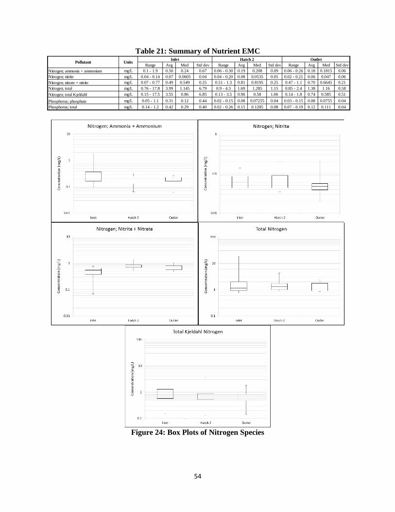
54
Table 21: Summary of Nutrient EMC
Figure 24: Box Plots of Nitrogen Species
Range Avg Med Std dev Range Avg Med Std dev Range Avg Med Std dev
Nitrogen; ammonia + ammonium mg/L 0.1 - 1.9 0.50 0.24 0.67 0.06 - 0.30 0.19 0.208 0.09 0.06 - 0.26 0.18 0.1815 0.06
Nitrogen; nitrite mg/L 0.04 - 0.14 0.07 0.0605 0.04 0.04 - 0.20 0.08 0.0535 0.05 0.02 - 0.21 0.06 0.047 0.06
Nitrogen; nitrate + nitrite mg/L 0.07 - 0.77 0.49 0.549 0.25 0.51 - 1.3 0.81 0.8195 0.25 0.47 - 1.1 0.70 0.6645 0.21
Nitrogen; total mg/L 0.76 - 17.8 3.99 1.145 6.79 0.9 - 4.3 1.69 1.285 1.15 0.85 - 2.4 1.38 1.16 0.58
Nitrogen; total Kjeldahl mg/L 0.15 - 17.5 3.55 0.86 6.85 0.13 - 3.5 0.96 0.58 1.06 0.14 - 1.8 0.74 0.585 0.51
Phosphorus; phosphate mg/L 0.05 - 1.1 0.31 0.12 0.44 0.02 - 0.15 0.08 0.07255 0.04 0.03 - 0.15 0.08 0.0755 0.04
Phosphorus; total mg/L 0.14 - 1.2 0.42 0.29 0.40 0.02 - 0.26 0.15 0.1285 0.08 0.07 - 0.19 0.12 0.111 0.04
Inlet Hatch 2 OutletUnitsPollutant

55
Figure 25: Box Plots of Phosphorus Species
Table 22: Summary of Nutrient Statistical Analysis
Pollutant Paired T-Test Results (p<0.05)
Inlet - Hatch 2 Hatch 2 - Outlet Inlet - Outlet
Nitrogen; ammonia + ammonium
Nitrogen; nitrite
Nitrogen; nitrate + nitrite
Nitrogen; total
Nitrogen; total Kjeldahl
Phosphorus; phosphate
Phosphorus; total
Significant Decrease Significant Increase No Significance
No significant removal was observed for all nitrogen parameters. Analysing nitrogen by
its components yields some interesting results. The spread in concentration of observed ammonia
and ammonium was reduced, however the average change in concentration is insignificant. The
concentration of nitrite, and nitrate and nitrite fluctuate throughout the USDC but overall, change
is also insignificant. It is expected that the concentrations of ammonia, ammonium, and nitrite
will decrease and nitrate will increase, but there are not enough samples to confirm this with
statistics. The data suggests that the oxidation of ammonia may occur within the USDC either by
nitrifying bacteria or through natural processes. The median value at the outlet of ammonia and
ammonium is 181 μg/L, using the tables found in Ministry of Environment and Energy (1994)
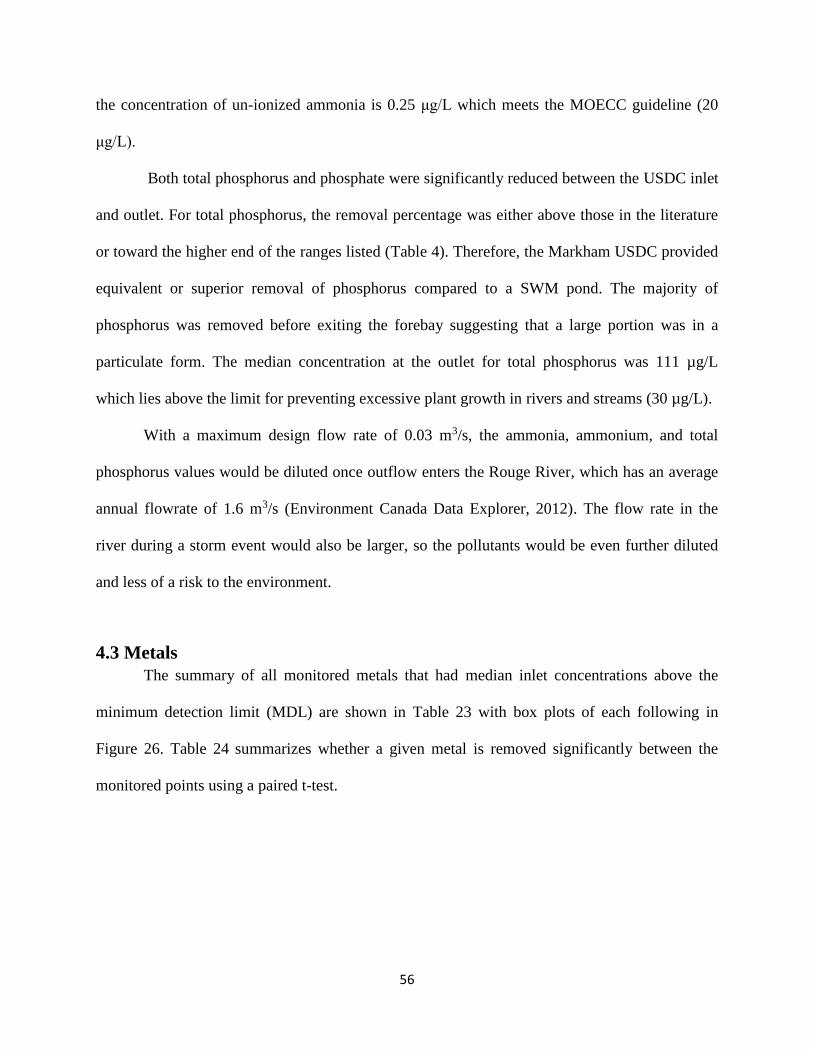
56
the concentration of un-ionized ammonia is 0.25 μg/L which meets the MOECC guideline (20
μg/L).
Both total phosphorus and phosphate were significantly reduced between the USDC inlet
and outlet. For total phosphorus, the removal percentage was either above those in the literature
or toward the higher end of the ranges listed (Table 4). Therefore, the Markham USDC provided
equivalent or superior removal of phosphorus compared to a SWM pond. The majority of
phosphorus was removed before exiting the forebay suggesting that a large portion was in a
particulate form. The median concentration at the outlet for total phosphorus was 111 µg/L
which lies above the limit for preventing excessive plant growth in rivers and streams (30 µg/L).
With a maximum design flow rate of 0.03 m3/s, the ammonia, ammonium, and total
phosphorus values would be diluted once outflow enters the Rouge River, which has an average
annual flowrate of 1.6 m3/s (Environment Canada Data Explorer, 2012). The flow rate in the
river during a storm event would also be larger, so the pollutants would be even further diluted
and less of a risk to the environment.
4.3 Metals
The summary of all monitored metals that had median inlet concentrations above the
minimum detection limit (MDL) are shown in Table 23 with box plots of each following in
Figure 26. Table 24 summarizes whether a given metal is removed significantly between the
monitored points using a paired t-test.

57
Table 23: Summary of Metals EMC
Figure 26: Box Plots of Monitored Metals
Range Avg Med Std dev Range Avg Med Std dev Range Avg Med Std dev
Aluminum ug/L 1200 - 7760 2740 1955 2490 364 - 2350 1120 925.5 622 126 - 1470 646 601 446
Antimony ug/L 0.3 - 0.6 0.47 0.5 0.10 0.4 - 0.7 0.51 0.5 0.12 0.4 - 3.9 1.06 0.7 1.16
Arsenic ug/L 0.6 - 1.5 1.00 1.05 0.32 0.8 - 1.2 1.04 1.05 0.14 0.7 - 1.3 0.90 0.8 0.19
Barium ug/L 28.7 - 135 62.8 53.2 38.24 31.4 - 68.8 46.3 46.45 11.33 23.5 - 44.7 32.1 32 6.55
Boron ug/L 23 - 36 30.3 31 4.76 30 - 58 40.6 41 8.67 25 - 44 35.4 35.5 7.03
Cobalt ug/L 1.1 - 5.4 2.22 1.7 1.63 0.5 - 2.5 1.13 0.9 0.62 0.2 - 1.3 0.63 0.65 0.35
Copper ug/L 6.7 - 22.6 14.6 13.75 6.06 6.5 - 10.3 7.78 7.55 1.24 4 - 8.4 6.44 6.85 1.57
Iron ug/L 870 - 8000 2450 1575 2748 400 -1660 920 780 416 110 - 1030 520 560 313
Lead ug/L 2.7 - 12.7 5.30 4.15 3.76 1.4 - 5.6 2.71 2.35 1.38 0.3 - 3.3 1.43 1.35 0.88
Manganese ug/L 76.4 - 393 175 137.2 120 39 - 283 113 91.5 74.78 10.8 - 130 46.4 41.4 37.44
Nickel ug/L 2.3 - 11.3 4.50 3.35 3.40 2.0 - 4.2 2.69 2.3 0.91 0.9 - 2.2 1.63 1.75 0.48
Strontium ug/L 126 - 281 208 201.5 58.14 223 - 379 286 274.5 48.74 158 - 303 226 220 45.64
Titanium ug/L 11.1 - 19.7 14.5 13.9 3.09 7.7 - 17.3 11.7 11.25 3.33 4.2 - 21.5 10.2 10.1 5.29
Vanadium ug/L 3.3 - 14.6 6.00 4.6 4.28 1.9 - 4.9 3.09 3 1.00 0.9 - 4.8 2.40 2.5 1.32
Zinc ug/L 16.2 - 106 45.3 35.25 32.00 14.5 - 37.5 21.7 20.55 7.11 6.5 - 21.3 13.0 12.85 5.13
OutletPollutant Units
Inlet Hatch 2

58
Figure 26: Box Plots of Monitored Metals (Continued)
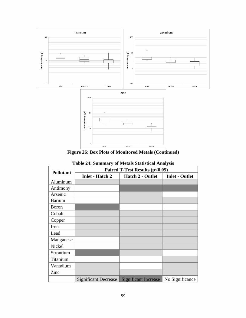
59
Figure 26: Box Plots of Monitored Metals (Continued)
Table 24: Summary of Metals Statistical Analysis
Pollutant Paired T-Test Results (p<0.05)
Inlet - Hatch 2 Hatch 2 - Outlet Inlet - Outlet
Aluminum
Antimony
Arsenic
Barium
Boron
Cobalt
Copper
Iron
Lead
Manganese
Nickel
Strontium
Titanium
Vanadium
Zinc
Significant Decrease Significant Increase No Significance

60
All of these metals were significantly reduced between the inlet and outlet, with the
exception of antimony, which significantly increased, and boron, arsenic, and strontium, which
were unaffected. Compared to the removal percentages cited in Section 2.2.3, the removal of
metals by the Markham USDC are either greater or within the same range of previously
published SWM pond studies (Table 8); the only exception is arsenic. Therefore, the Markham
USDC proved treatment either equivalent or superior for the removal of the metals with the
exception of arsenic. The notable metals with large inflow concentrations are aluminum and iron
which have median inflow concentrations of 1.955 and 1.575 mg/L, respectively. For
comparison, the United States Environmental Protection Agency has secondary drinking water
standards of 0.2 mg/L and 0.3 mg/L for aluminum and iron respectively (US EPA, 2015). At the
outlet, the majority of metals are meeting the provincial water quality requirements listed in
Table 9 with only aluminum, copper, and iron exceeding the required concentrations.
Boron and strontium were found to significantly increase in concentration after exiting
the forebay. These metals have been known to increase in concentration when draining through
permeable pavement, so the increase may be due to contact with the concrete structure (Toronto
and Region Conservation Authority, 2012c). The effectiveness of the permanent pool and the
forebay are inconsistent between metals, with significant removal and percent removal being
dependant on the individual metal (Table 25). This result is sensible since the association with
various particle sizes and dissolved portion is dependent on the individual metal.

61
Table 25: Percent Removal of Metals
Pollutant Fraction of Pollutants Removed (%)
Inlet - Hatch 2 Hatch 2 - Outlet Inlet - Outlet
Aluminum 59.1 17.3 76.4
Antimony -9.8 -117.9 -127.7
Arsenic -3.8 13.8 10.0
Barium 26.4 48.9 22.5
Boron -33.9 17.3 -16.6
Cobalt 49.2 22.6 71.8
Copper 46.8 9.2 56.0
Iron 62.4 16.4 78.8
Lead 49.1 24.1 73.2
Manganese 35.2 38.2 73.4
Nickel 40.3 23.6 63.9
Strontium -37.4 28.6 -8.8
Titanium 19.2 10.4 29.6
Vanadium 48.5 11.5 60.0
Zinc 52.2 19.1 71.3
4.4 Bacteria
A summary of all bacteria measured is shown in Table 26 below with box plots of each
following in Figure 27. Table 27 summarizes whether a given bacteria is removed significantly
between the monitored points using a paired t-test. One less sample was analysed for bacteria,
the August 16th event was not captured.
Table 26: Summary of Bacteria EMC
Range Avg Med Std dev Range Avg Med Std dev Range Avg Med Std dev
Escherichia coli c/100mL 64 - 7600 3480 3000 3398 4 - 6300 1330 130 2285 3.3 - 1400 446 220 544
Fecal streptococcus c/100mL 140 - 9100 3980 2800 4167 4 -2800 935 940 993.07 10 - 2600 641 380 899
Pseudomonas aeruginosa c/100mL 660 - 8300 2750 1400 3169 4 - 8300 1430 360 3038 20 - 720 246 170 222
Inlet Hatch 2 OutletPollutant Units

62
Figure 27: Box Plots of Monitored Bacteria
Table 27: Summary of Bacteria Statistical Analysis
Pollutant Paired T-Test Results (p<0.05)
Inlet - Hatch 2 Hatch 2 - Outlet Inlet - Outlet
Escherichia coli
Fecal streptococcus
Pseudomonas aeruginosa
Significant Decrease Significant Increase No Significance
For each bacteria the USDC removes a large fraction on average of those that entered the
inlet; however, the large range of values at all points in the USDC result in E. coli as the sole
bacteria significantly removed on average. At the outlet, the median concentration of E. coli was
212 c/100mL; this is above the maximum acceptable concentration for beach water in Ontario
which is 100 c/100 mL (City of Toronto, 2015). The median inflow and outflow concentrations

63
of E. coli in a wetland basin/retention pond is 869 and 196 c/100 mL, respectively (International
Stormwater BMP Database, 2014). This concentration is within the same range as those
measured at the Markham USDC outlet.
Reduced concentrations between the inlet and outlet suggest that the conditions inside of
USDC are not conducive to the reproduction of bacteria. This is most likely due to the
consistently cold water (Section 4.5) and ambient air temperature. Bacteria are also removed
from the water through sedimentation since they are predominantly attached to particles that
enter during a storm event. An overall removal percentage for each bacteria is difficult to
guarantee since the concentrations at all measured points are highly variable.
4.5 Temperature
The temperature in the USDC was recorded using a YSI monitor at Hatch 1 and a HOBO
Water Temperature Data Logger at Hatch 5; these were located approximately 0.04 m above the
bottom of the USDC, the results are shown in Figure 28 below. The gap in recorded inlet data
between October 24th and November 11th was caused by a temporary malfunction of the YSI
sensor.
Figure 28: YSI Temperature Results
0
5
10
15
20
25
30
01-06-14 01-07-14 31-07-14 30-08-14 29-09-14 29-10-14 28-11-14
Tem
per
ature
(⁰C
)
Inlet Outlet
1

64
As can be seen, the temperature at the outlet of the USDC is consistently less than what is
entering the inlet throughout the entire monitoring period. At the outlet, the temperature
increases steadily from 8oC to its highest around 13oC in October. The low temperatures at the
beginning of June correspond to the period when the permanent pool was refilling following the
Markham USDC cleaning on May 29th. The temperature begins to decrease as the year
progresses into November. The inlet temperature varies significantly more than the outlet. This is
due to storm events bringing heated runoff from impervious surfaces into the USDC. The cooler
ambient air temperature in the USDC then begins to cool the permanent pool that remains after
the event. The sensors at Hatch 1 and 5 recorded average temperatures of 14.5 and 12.5oC at the
inlet and outlet respectively. The temperature of the outflow eliminates the release of thermally
enriched runoff and it poses no threat to organisms in coldwater streams (Chu et al., 2009). It is
unclear whether the splashpad has an effect on the inflow temperature, but it follows the same
patterns as before the splashpad was activated so whatever effect it has is minimal.
The time period noted by circle 1 in Figure 28 experienced a sharp drop and rise in the
inlet temperature, and a sharp drop in the outlet temperature. The drop was caused by a storm on
November 24th that occurred during the night. Instead of being warmed by the impervious
surfaces, the runoff entered the USDC at a cold temperature. The permanent pool remained cool,
but the forebay pool temperature was increased as the ambient air temperature increased
throughout the day.
The USDC studied by Natarajan and Davis (2010) had an average outflow temperature
during July of 19.7 oC which is significantly more than the Markham USDC (11.4 oC). Natarajan
and Davis (2010) saw a mean reduction in temperature of 1.6oC and the Markham USDC on
average achieved a 3.5oC reduction. One possible reason for this discrepancy was that Natarajan

65
and Davis were studying a detention system that was composed of 6-122 cm interconnected
storage pipes with limited storage and detention. Therefore, the system had a shorter time for
cooling the stormwater and a smaller volume of cool stored water that would buffer some of the
elevated temperature runoff. Also, the inflow temperature is much higher for Natarajan and
Davis (mean of 21.7oC) while the Markham USDC inflow temperature was 14.9oC. The runoff
temperature combined with the small storage volume would result in stored water heating
quickly, and any cooling would be dependant on the ambient air temperature.
The HOBO temperature sensor took measurements not at the outlet, but towards the
bottom of the USDC, so there is the potential that a temperature gradient was occurring.
However, of the four temperature profiles conducted (discuessed further in Section 4.7), there is
little temperature gradient within the USDC. To better confirm this, additional profiles are still
needed through the summer months.
4.6 Hydrocarbons
Significance tests could not be conducted on several hydrocarbons since the minimum
detection limit (MDL) was too high. Therefore, removal of hydrocarbons could not be
determined. The number of samples below the MDL for each hydrocarbon is shown in Table 28.
The box plots were created using the MDL values (10 ng/L) from the results. A summary of all
monitored hydrocarbons that had inlet concentrations above the MDL are shown in Table 29
below with box plots of each following it in Figure 29.
Table 28: Number of Hydrocarbon Samples below the MDL
Hydrocarbon Number of Samples Below MDL
Inlet Hatch 2 Outlet
Phenanthrene 1/6 3/8 8/8
Fluoranthene 1/6 3/8 7/8
Pyrene 1/6 4/8 7/8
Napthalene 1/6 6/8 8/8
Fluorene 0/6 6/8 6/8
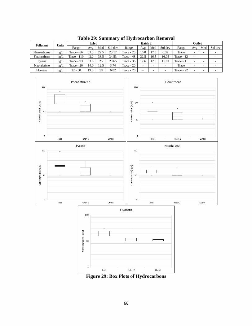
66
Table 29: Summary of Hydrocarbon Removal
Figure 29: Box Plots of Hydrocarbons
Range Avg Med Std dev Range Avg Med Std dev Range Avg Med Std dev
Phenanthrene ng/L Trace - 66 33.3 22.5 23.17 Trace - 25 16.8 17.5 6.32 Trace - - -
Fluoranthene ng/L Trace - 110 42.2 33.5 34.53 Trace - 48 22.5 16.5 16.05 Trace - 12 - - -
Pyrene ng/L Trace - 93 33.8 25 29.65 Trace - 36 17.6 12.5 11.01 Trace - 11 - - -
Naphthalene ng/L Trace - 20 14.0 12.5 3.74 Trace - 20 - - - Trace - - -
Fluorene ng/L 12 - 30 19.8 18 6.82 Trace - 26 - - - Trace - 22 - - -
UnitsInlet Hatch 2 Outlet
Pollutant

67
Lowering the MDL would have a more profound effect on those hydrocarbons with inlet
concentrations already close to the MDL, such as napthalene and fluorene. Unless a more
accurate test is conducted, the actual removal efficiency of hydrocarbons by USDC cannot be
determined. However, all of the concentrations at the outlet of the detected hydrocarbons are
below the provincial water quality requirements, with the exception of fluoranthene, which has a
requirement below the MDL. Each hydrocarbon and its associated requirement are listed in
Table 30.
Table 30: Hydrocarbon Provincial Water Quality Requirements
Hydrocarbon Provincial Water Quality
Requirement (μg/L)
Phenanthrene 0.03
Fluoranthene 0.0008
Pyrene N/A
Napthalene 7
Fluorene 0.2
Using the available data, the USDC appears to consistently remove a large portion of the
hydrocarbons after they pass through the forebay, only phenanthrene is significantly removed by
the forebay.
4.7 Vertical Profiles
Four vertical profiles of water quality have been taken since the USDC was installed at
the Markham site. Two of the profiles were taken before the cleaning of the USDC. The results
of the profile measurements are shown in Figure 30.

68
Figure 30: Depth Profile Results
Figure 30: Depth Profile Results (Continued)
The temperature and dissolved oxygen (DO) plots show that there is some stratification
occurring in the USDC (different values at different depths). Even though there is only a slight
decrease in temperature between the water surface and the bottom. There is a dramatic drop in
the DO saturation and concentration; this is suggestive of the presence of a thermocline which is
“the region in a thermally stratified body of water which separates warmer surface water from
cold deep water and in which temperature decreases with depth” (Merriam Webster, 2015).
0
0.2
0.4
0.6
0.8
1
1.2
1.4
1.6
0 5 10 15D
ep
th (
m)
Temperature C°
Jan 9/14 Mar 10/14
Dec 2/14 Feb 18/15
0
0.2
0.4
0.6
0.8
1
1.2
1.4
1.6
0 10 20 30
De
pth
(m
)
TDS (g/L)
Jan 9/14 Mar 10/14
Dec 2/14 Feb 18/15
0
0.2
0.4
0.6
0.8
1
1.2
1.4
1.6
0 20 40 60 80
De
pth
(m
)
Dissolved Oxygen Saturation (%)
Jan 9/14 Mar 10/14
Dec 2/14 Feb 18/15
0
0.2
0.4
0.6
0.8
1
1.2
1.4
1.6
0 5 10 15D
ep
th (
m)
Dissolved Oxygen Concentration (mg/L)
Jan 9/14 Mar 10/14
Dec 2/14 Feb 18/15

69
Thermoclines prevent the mixing of surface waters with those below, which induces a sharp
gradient in the DO concentration. The lack of mixing can also be a barrier to particle settling.
The relative thermal resistance to mixing (RTRM) was calculated as follows (Song, et al.,
2013):
RTRM =
(𝜌𝑧2 − 𝜌𝑧1)
(𝜌4 − 𝜌5) (23)
where ρ4 and ρ5 are the water densities at 4 and 5oC (kg/m3), and ρz1 and ρz2 are the water
densities at the water depths z1 and z2 respectively (kg/m3). The RTRM in the USDC ranged
from -2.42 to 1.88 which is much lower than the average in the SWM ponds monitored by Song
et al. (2013) which ranged from 63.2 to 218. Therefore, the thermal stratification that is
occurring is to a much lesser degree than that of SWM ponds. However; the profiles by Song et
al. (2013) were conducted during the summer months while the ones at the Markham site were
solely taken during the winter.
The minimum acceptable concentration for dissolved oxygen concentration is variable
depending on the type of river, the values are shown in Table 31. Based on the two profiles taken
after the USDC cleaning (December 2nd and February 18th), the water in the USDC is below the
minimum acceptable DO concentration for protection of aquatic organisms at all depths. To gain
a better understanding of USDC thermal and DO stratification, more profiles should be taken
during the summer months and when storm events occur.
Table 31: Minimum Acceptable Dissolved Oxygen Concentration in Rivers for the
Protection of Aquatic Life (Canadian Council of Ministers of the Environment, 2015)
River Biota Concentration (mg/L)
Warm water: early life stages 6.0
Warm water: other life stages 5.5
Cold water: early life stages 9.5
Cold water: other life stages 6.5
70
The total dissolved solids (TDS) profile returned results as expected. A slight increase in
TDS at the bottom of the USDC would occur since all of the solids that were removed from
runoff settle to the bottom. The profiles taken on January 9th and March 10th 2014 have far
different results than the other two; these were taken before the USDC was cleaned, so there was
a high concentration of TDS in the permanent pool. Therefore, those profiles are not
representative of a USDC under working conditions.
4.8 Summary
The chapter discussed the results of the site runoff analysis and compared them to
standard SWM pond removal capabilities. Of the captured samples, six at the inlet and eight at
the outlet were usable. The sampled storm were deemed to be frequently occurring events (return
period ≤ 2 years) and so were within the design capacity of the Markham USDC.
TSS and turbidity were significantly removed by the Markham USDC. An 82.1% TSS
removal was achieved, therefore the Markham USDC achieved enhanced protection (80% TSS
removal) and is equivalent to SWM ponds for the removal of TSS. Lab testing was performed to
develop a relationship between turbidity and TSS, this relationship will be used to convert
turbidity measurements to TSS and then compare the measured TSS removal in a storm to the
modeled removal by MUDS.
No significant removal was observed for nitrogen parameters, a decrease in total nitrogen
occurs in SWM ponds and so was expected to occur in the Markham USDC. A decrease in
average concentration did occur but was not large enough to declare with statistical significance.
Phosphorus was significantly removed, the change in concentration was either equivalent or
greater than SWM ponds found in the literature. The effluent met the MOECC guideline for un-
71
ionized ammonia (20 μg/L) but not the total phosphorus guideline for preventing excessive plant
growth in rivers and streams (30 µg/L)
All metals were significantly removed between the inlet and outlet, with the exception of
antimony, arsenic, boron, and strontium. Of those removed, the change in concentration is either
greater or within the same range as SWM ponds found in the literature. A possible explanation
for the increase in concentration of some metals is extended contact time with concrete in the
USDC; the specific metals have been known to increase in concentration when draining through
permeable pavement (Toronto and Region Conservation Authority, 2012c). The concentrations
of metals in the effluent are meeting provincial water quality requirements other than aluminum,
copper, and iron.
Large ranges in values were found for each bacteria at all monitored points. The observed
concentrations are suggestive of a reduction in concentration but an overall removal percentage
is difficult to guarantee due to the high variability. Reduced concentrations between the inlet and
outlet suggest the conditions inside the Markham USDC are not conducive to the production of
bacteria. The median concentration of E. coli was above the maximum acceptable concentration
for beach water in Ontario.
Temperature was monitored from the beginning of June to the beginning of December.
Average temperature at Hatch 1 and Hatch 5 (inlet and outlet) were 14.5 and 12.5oC respectively.
The average decrease in temperature was expected due to the literature and known conditions of
the Markham USDC; this is an advantage over SWM ponds which are known to release elevated
temperature effluent. The temperature of the Markham USDC effluent poses no threat to
organisms in coldwater streams (Chu et al., 2009)

72
Statistical analysis of hydrocarbons could not be conducted due to a large number of non-
detects at Hatch 2 and the outlet. The observed concentrations are suggestive of a reduction in
concentration of hydrocarbons, the actual amount cannot be calculated. All of the concentrations
of measured hydrocarbons are below the provincial water quality requirement except
fluoranthene which has a requirement below the MDL.
Four vertical profiles were conducted during the winter months. Observing the
temperature and DO plots show that there is some stratification occurring in the Markham
USDC. The water in the Markham USDC is below the minimum acceptable DO concentration at
all depths. TDS concentration increases with depth as expected. The following chapter will
discuss the development of the SWMM model and MUDS and the results obtained through
performing simulations.

73
Chapter 5 Model Development and Results
Due to the various issues with clogging and the splashpad, as mentioned in
Section 3.1, only storms from September onwards were utilized for calibration and validation of
the SWMM model. A summary of key hydrological parameters for each storm is shown in Table
32. Assessment of MUDS was conducted using the storms listed in Table 32 with the exception
of those in November due to malfunctions with the turbidity meters at that time. The values used
for SWMM calibration and validation and in MUDS’ pollutant removal assessment are listed in
Table 33.
Table 32: Summary of Calibration and Validation Events
Event
Date
Duration
(hrs)
Depth
(mm)
Max
Intensity
(mm/hr)
Average Intensity
(mm/hr)
Preceding
Dry Days
Sep-02 3.0 26.6 67.2 8.6 10
Sep-05 11.8 42.6 79.2 3.6 3
Sep-10 10.8 25 16.8 2.3 4
Sep-13 4.5 2.8 4.8 0.6 2
Sep-15 3.4 3.2 4.8 0.9 2
Sep-21 2.8 21 52.8 7.2 <1
Oct-03 2.8 7 9.6 2.4 12
Oct-06 26.0 13.2 9.6 0.5 2
Oct-15 5.3 6.6 4.8 1.2 8
Oct-16 5.8 19.2 33.6 3.3 <1
Oct-20 12.6 9.6 7.2 0.8 4
Nov-06 9.8 5.8 4.8 0.6 2
Nov-17 5.1 8 4.8 1.5 6
Nov-24 6.8 18.6 12 2.7 2

74
Table 33: MUDS Input Values
USDC Property Value
Surface Area (m2) 854
Average Width (m) 12
Height to Outlet Orifice Invert (m) 1.38
Orifice Diameter (m) 0.15
Starting Height (m) 1.38
Starting Outflow (m3/s) 0
Pathlength (m) 80
Particle Density (kg/m3) 2650
Particle Size Distribution
d10 (μm) 0.8
d20 (μm) 1.2
d30 (μm) 1.6
d40 (μm) 2.2
d50 (μm) 3.1
d60 (μm) 4.5
d70 (μm) 6.6
d80 (μm) 10.6
d90 (μm) 19.2
First Flush Ratio (Pollutant Mass/Volume)
Percentage of Pollutants 50
Percentage of Flow 50
Overflow Outlets
Height to Outlet Orifice Invert 1 (m) 2.45
Orifice Diameter 1 (m) 0.525
Height to Outlet Orifice Invert 2 (m) 2.45
Orifice Diameter 2 (m) 0.525
Water Properties
Density (kg/m3) 998.21
Dynamic Viscosity (kg/m∙s) 0.001002

75
5.1 SWMM Calibration and Validation
Calibration of the SWMM model began by comparing the outflow calculated, using the
measured depth and the equations in Table 12, against measured outflow data for monitored
storms. One such comparison is shown in Figure 31. The NSE equation (Equation 17), was used
to determine what orifice diameter and orifice height provided the most accurate flow prediction.
Ideally, the orifice diameter and height from the design documents would be used, but there were
complications that required these numbers to be adjusted. Following the orifice plate clogging
event from late July to mid-August, when some leaking occurred around the plate, the model
orifice diameter was increased from 0.12 to 0.15 m in order to better simulate measured flow
rates. If the calculated outflow was not responding to the depth as predicted then that event was
not used for calibration or validation. The comparison was also used to determine whether there
was an issue with the orifice plate so that it could be remedied as soon as possible.
Figure 31: Measured and Modeled Outflow Comparison
Following the comparison of measured and modeled outflows, the rainfall data for each
storm was entered into the SWMM model and an inflow hydrograph to the USDC was
generated. These data were entered MUDS to predict outflows and water depths throughout the
storm event. The orifice diameter and depth values from the first comparison were used by
MUDS and the outputs were compared against the measured data using the NSE equation.
1400
1500
1600
1700
1800
0
5
10
15
20
25
30
02-09-14 03-09-14 04-09-14D
ep
th (
mm
)
Flo
w R
ate
(L/
s)
Q Measured Q Modeled USDC Depth

76
A total of 12 storms were used for calibration of the SWMM model. The subcatchment
parameters that were calibrated were the depth of storage for impervious and pervious surfaces,
and the percent of impervious surface area. A baseflow parameter was also adjusted for the
September 2nd, 5th, 10th, 13th, and 15th storms to account for flow from the splashpad, the average
of the first 10 timesteps of the measured flow before a storm event were used as the baseflow.
Figure 32 shows the results for the depth and outflow following calibration. The median
NSE values were 0.52 and 0.49 respectively. With the exception of two events (Oct 15th and Nov
17th), the calibration storms remained within satisfactory to good prediction range (0.36-0.75) as
recommended by Moriasi et al. (2007). The model overpredicted the flow rates for the Oct 15th
and Nov 17th event by a large proportion of the measured flow rate; however, the measured flow
rates are very low with the maximum rate being 2.2 and 2.4 L/s respectively. Therefore, the
apparently poor accuracy based on the NSE value is misleading since the model only
overestimated by 1 - 2 L/s.
Figure 32: Calibration Height and Flow Results
-5
-4
-3
-2
-1
0
1
2
Height Flow
NSE
Val
ue

77
Two storms, (Oct 16th and 20th) were used for validation of the SWMM model. The
measured versus modeled outflow and depth for each storm event are shown in Figure 33 to
Figure 36. The flow and depth figures for the storms used for calibration are included in
Appendix C.
Figure 33: October 16 Outflow Modeling
Figure 34: October 16 Depth Modeling
Figure 35: October 20 Outflow Modeling
0
0.02
0.04
0.06
0.08
0.1
0
5
10
15
20
0 2 4 6 8 10 12 14 16 18 20
Infl
ow
(m
3 /s)
Ou
tflo
w (
L/s)
Time (h)
NSE = 0.52
Qout Measured Qout Modeled Qin Modeled
1.34
1.44
1.54
1.64
0 2 4 6 8 10 12 14 16 18 20
De
pth
(m
)
Time (h)
NSE = 0.36
Depth Measured Depth Modeled
0
0.005
0.01
0.015
0.02
0
1
2
3
4
5
0 5 10 15 20 25 30 35 40 45
Infl
ow
(m
3 /s)
De
pth
(m
)
Time (h)
NSE = 0.46
Qout Measured Qout Modeled Qin Modeled

78
Figure 36: October 20 Depth Modeling
The outflow NSE values are close to the median of the calibration storm events but the
depth NSE values are much lower than expected. This is possibly due to differences in localized
rainfall between the monitoring site and the USDC catchment area, which are roughly 3 km
apart. This discrepancy is quite obvious when examining the October 16th storm which has a
brief intense spike in inflow with no outflow registered on the monitoring devices. Either the rain
that caused this spike did not occur at the USDC site or it was part of the second inflow spike.
Smaller spatial variations in rainfall may have occurred in the October 21st storm but to a much
lesser degree, since the flow rates resulting from this storm were also smaller.
In general, the modeled outflow and depth followed similar temporal patterns and slopes
relative to the measured data, with variations in quantity largely being responsible for low NSE
values. These variations were less severe in storms that solicited higher inflow rates since the
differences in local rainfall intensity would not have as large an effect on inflow rates. For
example, a difference in modeled to measured flow of 3 m3/s when the modeled value is 27 m3/s
does not have as severe an effect as a 3 m3/s difference when the modeled value is 10 m3/s. The
storm on October 16th was exceptional in that there was a localized intense downpour at the
1.34
1.36
1.38
1.4
1.42
1.44
0 5 10 15 20 25 30 35 40 45
De
pth
(m
)
Time (h)
NSE = 0.01
Depth Measured Depth Modeled
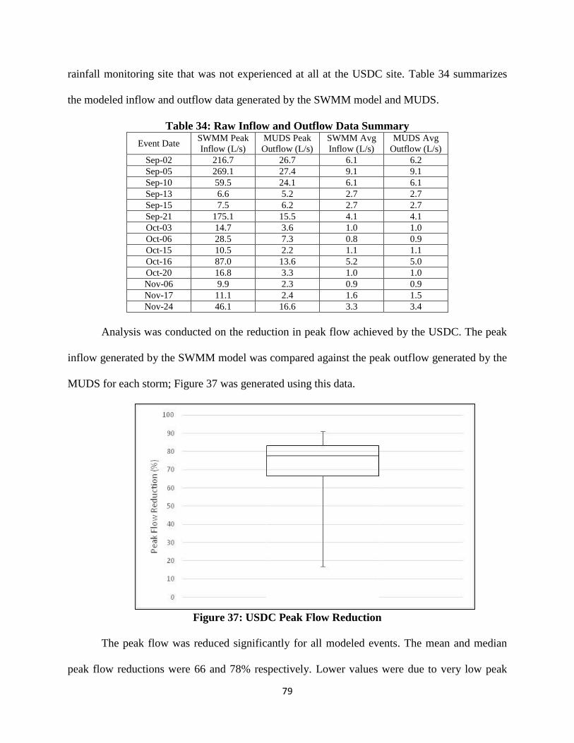
79
rainfall monitoring site that was not experienced at all at the USDC site. Table 34 summarizes
the modeled inflow and outflow data generated by the SWMM model and MUDS.
Table 34: Raw Inflow and Outflow Data Summary
Event Date SWMM Peak
Inflow (L/s)
MUDS Peak
Outflow (L/s)
SWMM Avg
Inflow (L/s)
MUDS Avg
Outflow (L/s)
Sep-02 216.7 26.7 6.1 6.2
Sep-05 269.1 27.4 9.1 9.1
Sep-10 59.5 24.1 6.1 6.1
Sep-13 6.6 5.2 2.7 2.7
Sep-15 7.5 6.2 2.7 2.7
Sep-21 175.1 15.5 4.1 4.1
Oct-03 14.7 3.6 1.0 1.0
Oct-06 28.5 7.3 0.8 0.9
Oct-15 10.5 2.2 1.1 1.1
Oct-16 87.0 13.6 5.2 5.0
Oct-20 16.8 3.3 1.0 1.0
Nov-06 9.9 2.3 0.9 0.9
Nov-17 11.1 2.4 1.6 1.5
Nov-24 46.1 16.6 3.3 3.4
Analysis was conducted on the reduction in peak flow achieved by the USDC. The peak
inflow generated by the SWMM model was compared against the peak outflow generated by the
MUDS for each storm; Figure 37 was generated using this data.
Figure 37: USDC Peak Flow Reduction
The peak flow was reduced significantly for all modeled events. The mean and median
peak flow reductions were 66 and 78% respectively. Lower values were due to very low peak

80
inflow rates and so the USDC could not reduce the outflow much further. The highest outflow of
the modeled events was 27.4 m3/s from the September 5th storm with a peak inflow of 269.1
m3/s. The average inflow and outflow rates were equivalent across the same timeframe
regardless of the decrease in peak flow. Therefore, the flow is released across a longer
timeframe.
5.2 Particle Removal Assessment
Assessment of MUDS’ particle removal model was conducted by comparing the modeled
removal to the mass load efficiency calculated from turbidity and flow data. The mass load
efficiency (Equation 4) requires inflow, outflow, and TSS concentration data for each time step
in order to estimate the fraction of pollutants removed. The concentration of TSS was determined
using the TSS to turbidity relationship presented in Section 4.1. The accuracy of the inflow
hydrograph generated by the SWMM model was highly variable and was considered an
ineffective tool to assess removal efficiency. Instead, the inflow hydrograph for each storm was
generated by performing a mass balance on the measured outflow hydrograph; the mass balance
equation is shown below.
𝑄𝑖𝑛 − 𝑄𝑜𝑢𝑡 =
𝛥ℎ ∗ 𝑆𝐴
𝛥𝑡 (25)
where Qin and Qout is flow in and out of the USDC (m3/s), Δh is change in height over time (m),
SA is surface area of the USDC (m2), and Δt is time over which the change in height occurs (s).
The various monitoring devices installed at the Markham USDC provided data for all the
variables in Equation 24 so an inflow hydrograph was easily generated. In the cases where the
mass balance resulted in a negative inflow, a value of zero was used instead since a negative
flow through the inlet is physically impossible. This situation occurs when there is a decrease in

81
height that is too large to be explained by the measured outflow, so mathematically there must be
flow out of the inlet; the discrepancy is most likely due to errors in measured outflow, depth,
and/or surface area. The generated inflow hydrograph was then entered in MUDS and
simulations were run to predict the particle removal percentage for several storm events.
In general, the accuracy of the flow and height prediction improved compared to the
results using SWMM inflow hydrographs. This method was most effective for storms with large
flow rates. Storms with flow rates below 5 m3/s were more affected by the replacement of
negative inflow with zero. In the cases where the accuracy of the new outflow hydrograph was
worse than the one from the SWMM model, the SWMM model outflow hydrograph was used for
pollutant removal assessment.
The first flush ratio for each storm was calculated by plotting the measured cumulative
mass/total mass against the inflow hydrographs cumulative volume/total volume. This graph was
compared against one where the cumulative mass/total mass was calculated using Equation 6
where the value of b was input by the user. The best fitting first flush ratio was determined using
the NSE equation (Equation 17). An example of this comparison is shown in Figure 38.
Figure 38: First Flush Ratio Calibration Example
PSD were determined by the MOECC lab, where water quality testing was conducted.
The average PSD across all sampled storms was used to run MUDS. This is shown in Table 33.
0
0.2
0.4
0.6
0.8
1
0 0.2 0.4 0.6 0.8 1
Cu
mu
lati
ve M
ass/
Tota
l Mas
s
Cumulative Volume/Total Volume
Measured Calculated

82
The PSD for this catchment is very fine compared to the mixed-residential PSD found by the
Toronto and Region Conservation Authority (2012a). Therefore, particles in runoff from the
Markham catchment area are expected to take longer to settle and to be more difficult to remove
compared to “typical” Toronto catchments. Consequently, lower removal rates of TSS are
expected from the Markham USDC. The TRCA PSD and average PSD across monitored storms
is provided in Table 35, with a graphical representation following in Figure 39.
Table 35: TRCA and Average Monitored Storm PSD
Particle
Diameter TRCA
Average
Monitored Storm
d10 (μm) 3.4 0.8
d20 (μm) 5.8 1.2
d30 (μm) 7.8 1.6
d40 (μm) 10.2 2.2
d50 (μm) 12.5 3.1
d60 (μm) 16.2 4.5
d70 (μm) 19.8 6.6
d80 (μm) 26.2 10.6
d90 (μm) 46.7 19.2
Figure 39: TRCA and Average Monitored Storm PSD
When conducting the assessment of the MUDS particle removal predicion, preliminary
monitored removal rates calculated using the real-time turbidity measurements were returning
consistently lower values than those of the model. Upon closer inspection it was found that a
0
20
40
60
80
100
0 10 20 30 40 50
Pe
rce
nt
Smal
ler
Than
Particle Diameter (μm)
TRCA Average Monitored Storm
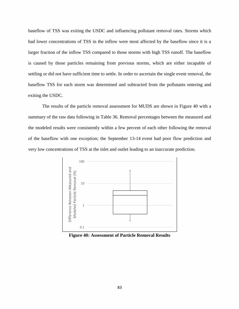
83
baseflow of TSS was exiting the USDC and influencing pollutant removal rates. Storms which
had lower concentrations of TSS in the inflow were most affected by the baseflow since it is a
larger fraction of the inflow TSS compared to those storms with high TSS runoff. The baseflow
is caused by those particles remaining from previous storms, which are either incapable of
settling or did not have sufficient time to settle. In order to ascertain the single event removal, the
baseflow TSS for each storm was determined and subtracted from the pollutants entering and
exiting the USDC.
The results of the particle removal assessment for MUDS are shown in Figure 40 with a
summary of the raw data following in Table 36. Removal percentages between the measured and
the modeled results were consistently within a few percent of each other following the removal
of the baseflow with one exception; the September 13-14 event had poor flow prediction and
very low concentrations of TSS at the inlet and outlet leading to an inaccurate prediction.
Figure 40: Assessment of Particle Removal Results
0.1
1
10
100
Dif
fere
nce
Bet
wee
n M
easu
red
an
d
Mo
del
ed P
arti
cle
Rem
ova
l (%
)

84
Table 36: Assessment of Particle Removal Summary Storm Event Modeled Particle Removal Measured Particle Removal
September 2-4 100 97.1
September 5-7 100 95.3
September 10-12 100 95.1
September 13-14 100 62.0
September 15-16 100 95.3
September 21-22 100 98.1
October 3-4 100 99.8
October 6-9 100 99.5
October 15-16 100 96.2
October 16-17 100 99.7
October 20-21 100 99.7
The storms used for assessment all resulted in a predicted removal of 100% of the
particles; therefore, the flow rates and lengths of the storms were not large enough to move
particles from the inlet to the outlet in a single event. While this is problematic for assessing the
accuracy of removal in larger storms, the results do match well with the monitored events after
removing the baseflow from the measured values.
5.2.1 Sensitivity Analysis Sensitivity analysis was conducted on the variables that govern particle removal in
MUDS. The results are shown in Figure 41. The July to August time period was selected for
sensitivity simulations.
Figure 41: Sensitivity Analysis Results
65
70
75
80
85
90
-20% -10% Zero 10% 20%
Par
ticl
e R
em
ova
l Eff
icie
ncy
(%
)
Particle Density USDC Surface Area

85
The original values for particle density, surface area, and length used by MUDS (Table
33) were scaled by -20, -10, 10, and 20% to determine what effect they had on the TSS removal
percent. The length appears to have the largest effect on particle removal. This is intuitive, since
the pathlength of the particle is directly related to how long it has to settle in the USDC. The
surface area has the least effect; it indirectly changes the particle removal by altering the
hydraulics of the USDC.
The three properties all follow linear trends within this ±20% range. The +10% length
value is the only exception. The cause of this discrepancy is most likely due to assumptions
made by MUDS, in particular, the assumption explained in Appendix B – B.4 where the particle
exit height is greater than entry height; this situation may occur several times during the July to
August time period as there are storms which cause a large increase in depth very quickly. If a
large mass of pollutants are present at the very end of the USDC, then they will exit at a height
greater than the entry height which will provide a more conservative removal percentage than
what is actually occurring. Sensitivity analysis of the pathlength was conducted again using the
September – November time period. It was found to follow a linear trend which reinforces the
conclusion that the non-linear trend is a highly situational error based on MUDS’ assumptions.
5.3 Markham USDC MUDS Simulations
5.3.1 Design Storm Simulation In order to determine how well the USDC performs under extreme conditions, two design
storms were simulated with MUDS. Five and ten year storm events with rainfall duration of 2
hours were used; this corresponds to average rainfall intensities of 17.3 mm/hr and 20.2 mm/hr,
respectively (Ministry of Transportation, 2013). The five and ten year events are common design
criteria for quantity control for Ontario municipalities and a 2 hour storm period was selected to

86
test the most extreme conditions for five and ten year storms. For the purposes of this thesis, the
return period of a storm is defined using the average rainfall intensity across a storm event. The
rainfall intensities were assumed to be constant over two hours and were input to the SWMM
model to develop an inflow hydrograph. A first flush ratio of 80/30 was used to predict a highly
concentrated release of pollutants. The designed outlet diameter of 0.12 m was used instead of
the 0.15 m for calibration and validation to evaluate how the USDC acts under designed
conditions. The outflow and inflow hydrographs are shown in Figure 42 and Figure 43.
Figure 42: 5 Year Storm Hydrographs
Figure 43: 10 Year Storm Hydrographs
The peak flow was reduced substantially. The 10 year return period event outflow is well
below the maximum design outflow of 30 L/s, which was the outflow for a 5 year return period
storm. Therefore, the Markham USDC exceeds all hydraulic expectations for reducing peak
0
20
40
60
80
100
120
0 5 10 15 20 25 30
Flo
wra
te (
L/s)
Time (h)
Qout
Qin
0
20
40
60
80
100
120
140
0 5 10 15 20 25 30
Flo
wra
te (
L/s)
Time (h)
Qout
Qin
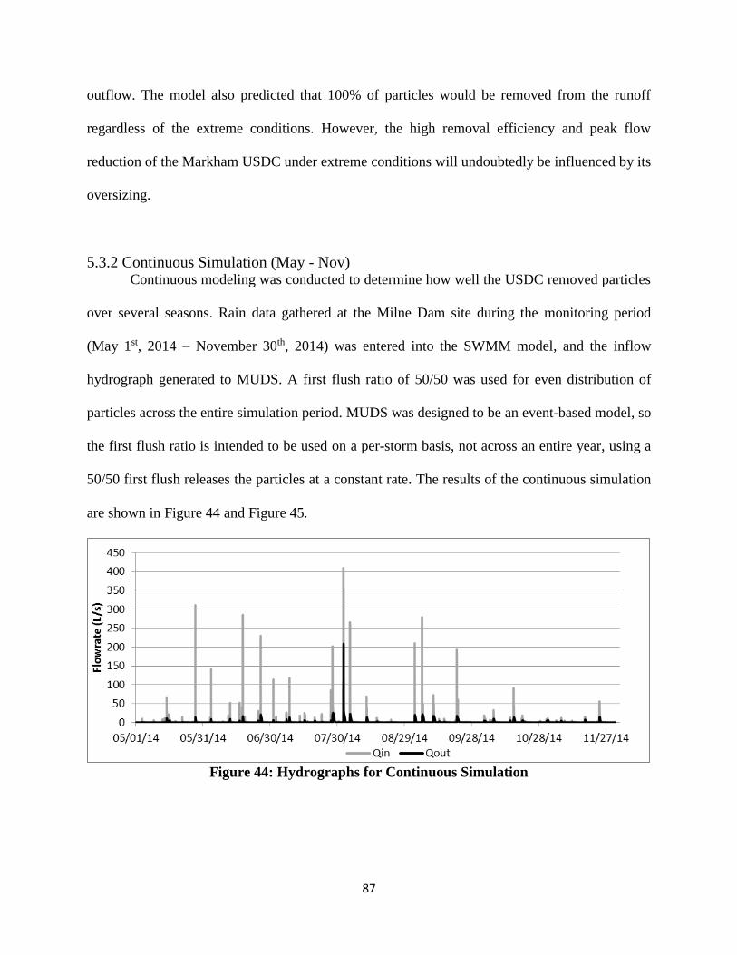
87
outflow. The model also predicted that 100% of particles would be removed from the runoff
regardless of the extreme conditions. However, the high removal efficiency and peak flow
reduction of the Markham USDC under extreme conditions will undoubtedly be influenced by its
oversizing.
5.3.2 Continuous Simulation (May - Nov) Continuous modeling was conducted to determine how well the USDC removed particles
over several seasons. Rain data gathered at the Milne Dam site during the monitoring period
(May 1st, 2014 – November 30th, 2014) was entered into the SWMM model, and the inflow
hydrograph generated to MUDS. A first flush ratio of 50/50 was used for even distribution of
particles across the entire simulation period. MUDS was designed to be an event-based model, so
the first flush ratio is intended to be used on a per-storm basis, not across an entire year, using a
50/50 first flush releases the particles at a constant rate. The results of the continuous simulation
are shown in Figure 44 and Figure 45.
Figure 44: Hydrographs for Continuous Simulation
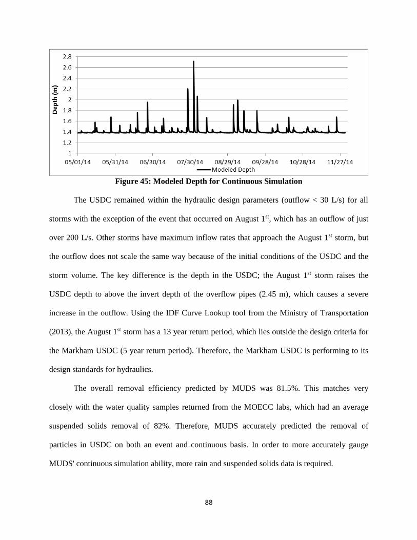
88
Figure 45: Modeled Depth for Continuous Simulation
The USDC remained within the hydraulic design parameters (outflow < 30 L/s) for all
storms with the exception of the event that occurred on August 1st, which has an outflow of just
over 200 L/s. Other storms have maximum inflow rates that approach the August 1st storm, but
the outflow does not scale the same way because of the initial conditions of the USDC and the
storm volume. The key difference is the depth in the USDC; the August 1st storm raises the
USDC depth to above the invert depth of the overflow pipes (2.45 m), which causes a severe
increase in the outflow. Using the IDF Curve Lookup tool from the Ministry of Transportation
(2013), the August 1st storm has a 13 year return period, which lies outside the design criteria for
the Markham USDC (5 year return period). Therefore, the Markham USDC is performing to its
design standards for hydraulics.
The overall removal efficiency predicted by MUDS was 81.5%. This matches very
closely with the water quality samples returned from the MOECC labs, which had an average
suspended solids removal of 82%. Therefore, MUDS accurately predicted the removal of
particles in USDC on both an event and continuous basis. In order to more accurately gauge
MUDS' continuous simulation ability, more rain and suspended solids data is required.

89
5.3.3 Seasonal Simulations MUDS was also run to determine how well the USDC removes particles on a seasonal
basis. Three time periods were selected: May-June, July-August, and September-November. The
results of the simulations are presented in Table 37.
Table 37: Seasonal and Overall TSS Removal Simulation Results
Modeled Time Particle Removal
Efficiency (%)
May – June 98.4
July – August 77.8
September -
November 95.1
May - November 81.5
The USDC is able to provide enhanced protection under MOECC standards (80% TSS
removal) except for July-August where it is slightly below the requirement. This makes sense by
examining Figure 45, which shows that this was also the period when the USDC was at the
greatest depth and correspondingly experienced the largest volumes of inflow. Larger volumes
flowing into the USDC lead to longer drainage time and consequently a higher probability that
particles which entered during the storm event or are already present in the USDC will reach the
outlet before settling.
The seasonal rainfall characteristics are an important factor to consider when designing a
USDC. While the Markham USDC achieves an overall removal of 81.5%, the July to August
time period does not meet the enhanced protection standard. If it is required that the USDC
achieve this standard at all times, then an overall removal is irrelavent and the designer should
instead focus on this critical time period where there is a combination of high inflow rates and
large inflow volumes.
Comparing the August 1st storm in Figure 46 to the same storm in Figure 44 shows that
there is a difference of around 70 L/s for the maximum inflow and 90 L/s for the maximum

90
outflow. Similar changes can also be observed in the other simulated storms. A change in the
inflow can only be explained by the conditions in the SWMM model, which in turn effects the
outflow. Investigating the runoff values calculated by SWMM revealed that each subcatchment
was releasing more runoff during the continuous simulation. The source of this error could not be
determined. The removal efficiency using the inflow and outflow rates from the May-November
simulation would most likely be lower than what was found using the July-August simulation.
Figure 46: July to August Simulation Hydrograph
5.3.4 Sizing Simulations Finally, MUDS was used to compare how well runoff would have been treated from the
Markham catchment area if the USDC had been sized for the correct catchment area (5.24 ha),
rather than the original area (7.97 ha). The surface area, average width, and length of the USDC
were reduced by the same factor as the contributing area, to roughly 65.7% (5.24/7.97) of the
original value. MUDS was run using these new values to determine if the USDC still meets the
hydraulic and runoff treatment requirements. The July-August time period was used to develop
the inflow hydrograph to determine the performance under the most intense rainfall conditions.

91
Figure 47: July to August New Area Hydrographs
The results of the simulation are shown in Figure 47. The changes have a profound effect
on the outflow rates calculated by the USDC. This change most notably occurrs in the August 1st
event where the outflow increases from the original July-August simulation (120 L/s) to just
under 200 L/s. The other storms remain under the hydraulic requirements. The reduction in
length and width drastically reduces the removal efficiency of suspended solids, the new USDC
achieves a removal of 51.2% compared to the original 77.8%.
Another simulation was run with the mixed commercial-residental PSD found by the
Toronto and Region Conservation Authority (2012a). This is shown in Table 35. While the
outflow hydrograph remains the same, the removal efficiency of suspended solids improves from
51.2% to 67.1% with the new PSD. This value is still well below the requirments for enhanced
protection under MOECC standards, indicating that a USDC can not be simply scaled based on
the catchment area. An iterative process is required to determine the appropriate dimensions for
the chamber.
This process was performed using the July-August time period to determine what
dimensions would be needed for the USDC for the reduced catchment area (5.24 ha) and the
TRCA PSD. Surface area, width, and length were all reduced to 80% and 85% of their original
values, resulting in a TSS removal efficiency of 79.1% and 84% respectively. Therefore, a

92
USDC with 85% of the original USDC properties is required for enhanced protection. The
hydraulic results are shown in Figure 48. These would be the required USDC measurements to
achieve enhanced protection during the worst time period of the year. Performing this process
using the May-November inflow hydrographs would likely result in a smaller USDC being
necessary.
Figure 48: Reduced Catchment Area with TRCA PSD Hydrographs
5.4 Summary
The chapter discussed the calibration and validation of the SWMM model hydraulics and
hydrology, the assessment of the pollutant removal modeling, and the results of several
simulations by MUDS. Due to various issues with clogging and the splashpad, only storms from
September onwards were utilized for the modeling process.
The SWMM model was calibrated and validated to ensure adequate simulation of the
hydraulics of the Markham USDC catchment. The NSE equation was used to compare measured
and modeled values. It was found that the SWMM model was more accurate for storms with
larger flow rates, NSE values for smaller flow rate storms were disproportionately affected by
small differences in modeled flow rate. Localized variations in rainfall may be partially
responsible for errors since the Markham USDC and rainfall monitoring site were 3 km apart.
The median modeled outflow and depth were within satisfactory to good prediction range (0.36 –
0.75) as recommended by Moriasi et al. (2007). Analyzing the hydraulic data revealed that the

93
Markham USDC reduced peak flow significantly for all modeled events. The mean and median
peak flow reductions were 66.1 and 77.6% respectively.
Assessment of MUDS’ particle removal model was conducted by comparing the modeled
removal to the mass load efficiency calculated from turbidity and flow data. First flush ratio was
determined on a per storm basis using measured turbidity data and the average PSD across
monitored storm was used. Removal percentages between the measured and modeled results
were consistently within a few percent of each other with one exception. The modeled storms
were not large enough to move particles from the inlet to outlet in a single event; however, the
results show that MUDS is accurate for predicting the removal of contaminants on an event
basis.
Several simulations were performed to determine the treatment and hydraulic capability
of the Markham USDC. A 5 and 10 year storm were input to the SWMM model to develop
inflow hydrographs, a first flush ratio of 80/30 was used to predict a highly concentrated release
of pollutants. Peak flows for both storms were below the maximum design outflow of 30 L/s and
no particles from the storm escaped over the duration of the event. Therefore, the Markham
USDC is performing above its design capacity for hydraulics and removal of TSS.
Continuous modeling was conducted to determine the accuracy of MUDS over an
extended time period and how well the Markham USDC removed particles over several seasons.
Rain data gathered at the Milne Dam site during the monitoring period was input to the SWMM
model. The Markham USDC met the hydraulic requirements except on one occasion where a
12.9 year storm occurred, this is beyond the design capacity of the Markham USDC and so is an
acceptable failure. MUDS predicted a removal efficiency of 81.5% which matches very closely

94
with the water quality results (82.1%). Therefore, MUDS is accurate for both event based and
continuous based modeling simulations.
Seasonal simulations were performed to determine whether the time of year has an effect
on USDC performance. The Markham USDC was found to perform worse during the July-
August time period, it was unable to achieve enhanced protection during this simulation. The
poorer performance during this time period was expected as the summer is when more and
higher intensity storms occur.
Finally, sizing simulations were performed on the Markham USDC, it was originally
designed for a 7.97 ha catchment but the contributing area was reduced to 5.24 ha after
installation. MUDS was used to determine the appropriate size by scaling the surface area, width,
and pathlength equally by the ratio of the areas (5.24/7.97). The predicted removal percentage
was 51.2%, the poor performance may have been due to the very find PSD of the Markham site.
Replacing the PSD with one found in the literature resulted in a removal of 67.1%. The surface
area, width, and pathlength were scaled equally to determine the size required for enhanced
protection. The parameters were scaled to 85% of their original values to achieve enhanced
protection; therefore, USDC cannot be scaled by catchment area, they require iterative use of
MUDS to determine appropriate sizing. The conclusions and recommendations from the work on
this thesis are discussed in the following chapter.
95
Chapter 6 Conclusions and Recommendations
6.1 Conclusions
The purpose of this research was to gain an understanding of how a USDC acts in an
Ontario climate. In the following sections, conclusions which address the research objectives will
be discussed. In summary, the research objectives were to:
1. Identify the stormwater treatment capabilities of USDC using on-site monitoring
2. Compare the runoff treatment from USDC to SWM ponds
3. Create a model that predicts the removal of contaminants in USDC
6.1.1 Objective 1 The stormwater treatment capabilities of a newly constructed StormTrap-DoubleTrapTM
were studied using field monitoring equipment installed in Markham, Ontario. This includes
ISCO samplers at the inlet, Hatch 2, and outlet, and YSI monitors at the inlet and outlet.
Monitoring and maintenance was performed by TRCA technicians from May-December 2014.
Samples were captured by the ISCO samplers during storm events; of those, six at the inlet and
eight at Hatch 2 and the outlet were used for water quality analysis. The Markham USDC was
found to provide peak flow reduction and water quality benefits for many monitored pollutants.
1. The USDC achieved an overall 82% removal efficiency of TSS which meets
enhanced protection requirements under MOECC standards (80% removal).
2. The average un-ionized ammonia concentration of 0.25 μg/L was below the MOECC
guideline of 20 μg/L, but total phosphorus far exceeded its guideline (30 μg/L) with
an average concentration of 111 μg/L.
96
3. All monitored metals achieved the provincial water quality requirements for
maximum allowable concentration (MAC) with the exception of aluminum, copper,
and iron.
4. The concentration of E. coli decreased significantly from the inlet to outlet, but the
median E. coli concentration of 212 c/100mL was greater than the MAC for beach
water in Ontario (100 c/100mL).
5. Temperatures were reduced significantly, with an average at the inlet and outlet of
14.5 and 12.5 oC, respectively.
6. Hydrocarbons were also removed very well, with few samples testing above the
MDL. All hydrocarbons met the provincial water quality requirements with the
exception of fluorene, which has a requirement below the lab MDL.
7. Several depth profile measurements taken showed that there was a slight temperature
gradient and a dissolved oxygen gradient between the surface and bottom of the
USDC.
Statistical analysis was performed to ascertain where the majority of removal was
occurring in the USDC for each individual pollutant. Understanding this assists in the design
process by determining whether the key design factor is the forebay or permanent pool. The
results for pollutants which were significantly removed are summarized in Table 38.

97
Table 38: Summary of Forebay and Residence Time Significance Tests
Pollutant Paired T-Test Results (p<0.05)
Inlet - Hatch 2 Hatch 2 - Outlet Inlet - Outlet
Total Suspended Solids
Turbidity
Nitrogen; ammonia + ammonium
Nitrogen; nitrate + nitrite
Nitrogen; total
Nitrogen; total Kjeldahl
Phosphorus; phosphate
Phosphorus; total
Aluminum
Antimony
Arsenic
Barium
Boron
Cobalt
Copper
Iron
Lead
Manganese
Nickel
Strontium
Titanium
Vanadium
Zinc
Phenanthrene N/A N/A N/A
Fluoranthene N/A N/A N/A
Pyrene N/A N/A N/A
Napthalene N/A N/A N/A
Fluorene N/A N/A N/A
Escherichia coli
Fecal streptococcus
Pseudomonas aeruginosas
Significant Decrease Significant Increase No Significance
6.1.2 Objective 2 The results of the pollutant removal analysis were MUDS compared against SWM ponds
to determine whether USDC provide an equivalent level of treatment. Values were taken from
various sources in the literature.
1. The removal of TSS by USDC was found to be equivalent to that of SWM ponds.

98
2. Phosphorus removal was either above or equivalent to listed removal rates in SWM
ponds.
3. The removal of metals by USDC are either greater or within the same range of
previously published studies with the exception of arsenic.
4. Effluent concentrations of E. coli were roughly equivalent to SWM ponds.
5. Runoff temperature was significantly reduced between the inlet and outlet whereas
SWM ponds consistently release water at an elevated temperature.
Overall, USDC have exhibited pollutant removal efficiencies at a greater or equivalent
level as SWM ponds.
6.1.3 Objective 3 The Model for Underground Detention of Sediment (MUDS) was developed by Nicholas
McIntosh at the University of Toronto. It has shown to be an accurate model for the prediction of
hydraulics and TSS removal for both event and continuous-based modeling. A sensitivity
analysis was performed on the suspended solids removal and it was found that changes in
particle pathlength have the greatest effect on removal percentage. MUDS was also used to
determine seasonal and particle size distribution effects on USDC performance. The findings of
the modeling process are as follows:
1. The Markham USDC remained beneath the required outflow rate of 30 L/s for 5 and
10 year storms with periods of 2 hours. The removal percentage for these storm
events was 100%.
2. Under continuous simulation from May - November the Markham USDC removed
81.5% of particles. There was one failure event where the outflow exceeded 30 L/s,
but this was during a 13 year return period storm which is outside the design capacity
of the USDC.
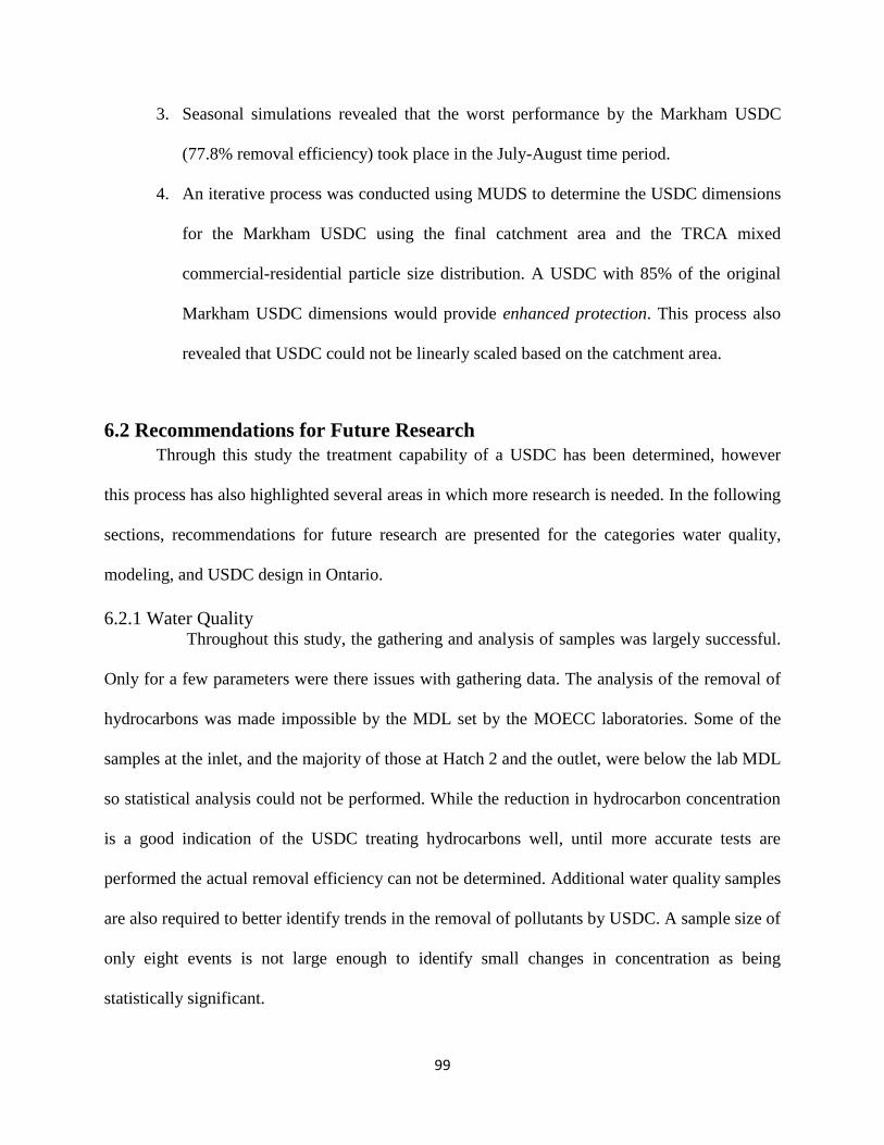
99
3. Seasonal simulations revealed that the worst performance by the Markham USDC
(77.8% removal efficiency) took place in the July-August time period.
4. An iterative process was conducted using MUDS to determine the USDC dimensions
for the Markham USDC using the final catchment area and the TRCA mixed
commercial-residential particle size distribution. A USDC with 85% of the original
Markham USDC dimensions would provide enhanced protection. This process also
revealed that USDC could not be linearly scaled based on the catchment area.
6.2 Recommendations for Future Research
Through this study the treatment capability of a USDC has been determined, however
this process has also highlighted several areas in which more research is needed. In the following
sections, recommendations for future research are presented for the categories water quality,
modeling, and USDC design in Ontario.
6.2.1 Water Quality Throughout this study, the gathering and analysis of samples was largely successful.
Only for a few parameters were there issues with gathering data. The analysis of the removal of
hydrocarbons was made impossible by the MDL set by the MOECC laboratories. Some of the
samples at the inlet, and the majority of those at Hatch 2 and the outlet, were below the lab MDL
so statistical analysis could not be performed. While the reduction in hydrocarbon concentration
is a good indication of the USDC treating hydrocarbons well, until more accurate tests are
performed the actual removal efficiency can not be determined. Additional water quality samples
are also required to better identify trends in the removal of pollutants by USDC. A sample size of
only eight events is not large enough to identify small changes in concentration as being
statistically significant.

100
Further research is also required on vertical profiles taken in USDC to determine the
existence and extent of thermal and dissolved oxygen stratification during the summer months.
The summer is when the USDC will be most active, so it is important to determine the
characteristics of the water being released during that time. If there is thermal stratification
during the summer, this may bring into question the thermal benefits provided by USDC. The
strong stratification of dissolved oxygen may also be different in the summer months since the
USDC will be receiving more inflow and so will be more turbulent.
The long term performance of USDC must also be studied. This monitoring program
took place over a single year, in order to ascertain the treatment capability of USDC over it's
lifetime a long term study should be conducted. This would also assist in determining the long
term maintenance requirements for sediment and debris cleanout. Extended monitoring can also
be used to determine whether the accumulation of sediment has an effect on the hydraulics or
treatment process of USDC.
6.2.2 Modeling Additional data is required to confirm the accuracy of MUDS for event and continuous
based simulation. For event-based simulations, larger events that result in particles flowing from
the inlet to the outlet in a single event are required before a non-100% removal will occur. For
continuous based, more data available for conducting simulations will increase the confidence in
prediction accuracy. Extended study of USDC may also reveal that accommodations must be
made for the accumulation of sediment and hydraulic losses.
The TSS removal simulated by MUDS could be expanded to include the removal of
pollutants strongly associated with TSS such as nutrients and metals. This also requires more

101
data, as the relationships between dissolved and particle fractions are complex and dependant on
the individual pollutant.
6.2.3 USDC Design in Ontario Through the course of the monitoring program it has become apparent that orifice plates
are not a practical solution to flow rate management on their own. The orifice plate installed on
the Markham USDC site clogged twice in quick succession due to plastic bags entering the
system with runoff. The clogging disrupted flow through the USDC and caused damage to the
orifice plate, resulting in noticeable leaking and a higher flow rate than designed. Without the
ongoing monitoring program, the clogging would not have been noticed and likely would have
persisted until the next maintenance period.
There are several solutions to preventing orifice clogging in SWM ponds such as a
submerged reverse-slope pipe, a trash rack, and a perforated pipe with wire cloth and stone
jacket (Greater Vancouver Sewerage and Drainage District, 1999). The most practical solution
would be to place a finely meshed grate across the opening from the forebay to the permanent
pool. The mesh would be sized such that any object small enough to pass through would not clog
the orifice plate. This solution would prevent any disruption to flow through the USDC and
miscellaneous garbage and debris would be confined to the forebay but adds another component
to the maintenance of USDC.

102
References
Adams, & Papa. (2000). Urban Stormwater Management Planning with Analytical Probabilistic Models. Chichester: John Wiley & Sons Ltd.
Agrawal, & Bewtra. (1985). Modified Approach to Evaluate Column Test Data. Journal of Environmental Engineering, 111(2): 231-234.
AZO Materials. (2007). Effect of Particle Size on The Taste, Texture and Manufacture of Chocolate Products, Particle Size Analysis Using The Micrometics DigiSizer.
Barrett, Irish, Malina, & Charbeneau. (1998). Characterization of Highway Runoff in Austin, Texas. Journal of Environmental Engineerin, 124: 131-137.
Bertrand-Krajewski, Chebbo, & Saget. (1998). Distribution of Pollutant Mass Vs. Volume in Stormwater Discharges and the First Flush Phenomenon. Water Resources, 32(8): 2341-2356.
Brater, King, Lindell, & Wei. (1996). Handbook of Hydraulics for the Solution of Hydraulic Engineering Problems 7th Edition. McGraw-Hill.
Buren, Watt, & Marsalek. (1997). Application of the Log-Normal and Normal Distributions to Stormwater Quality Parameters. Water Resources, 31(1): 95-104.
Canadian Council of Ministers of the Environment. (2015, April 2). Water Quality for the protection of Aquatic Life. Retrieved from Canadian Council of Ministers of the Environment: http://st-ts.ccme.ca/en/index.html?lang=en&factsheet=154#aql_fresh_concentration
Center for Hazardous Substance Research. (2009). Human Health Effects of Heavy Metals. Environmental Science and Technology Briefs for Citizens, 1-6.
Chin. (2013). Water-Resources Engineering. New Jersey: Pearson Education, Inc. Chu, Jones, Piggott, & Buttle. (2009). Evaluation of a Simple Method to Classify the Thermal
Characteristics of Streams Using a Nomogram of Daily Maximum Air and Water Temperatures. North American Journal of Fisheries Management, 29: 1605-1619.
City of Toronto. (2015, January). About Toronto Beaches Water Quality. Retrieved from toronto.ca: http://www.toronto.ca/health/swimsafe/beaches_about.htm
DeMartino, DePaola, Fontant, Marini, & Ranucci. (2011). Pollution Reduction in Receivers: Storm-Water Tanks. Journal of Urban Planning and Development, 137: 29-38.
Environment Canada. (2014, 02 10). Reducing Phosphorus Loads to Lake Simcoe. Retrieved from Environment Canada: http://www.ec.gc.ca/indicateurs-indicators/default.asp?lang=en&n=90435A23-1
Environment Canada Data Explorer. (2012, Nov 15). Environment Canada. Environmental Protection Agency SWMM 5.1 a. (2015). Surface Runoff. In E. P. Agency, EPA SWMM
Help. Environmental Protection Agency SWMM 5.1 b. (2015). Kinematic Wave Routing. In E. P. Agency, EPA
SWMM Help. Freeze, & Cherry. (1979). Groundwater. Englewood Cliffs, N.J.: Prentice-Hall. German, & Svensson. (2002). The Relation Between Stormwater and Sediment Quality in Stormwater
Ponds. Urban Drainage. Greater Vancouver Sewerage and Drainage District. (1999). Best Management Practices Guide for
Stormwater. Gross, D. (2015, April 17). General Sales Manager for Special Projects - StormTrap. (N. McIntosh,
Interviewer) Hallberg. (2006). Suspended Solids and Metals in Highway Runoff-Implications for Treatment Systems.
KTH Architecture and the Built Environment.

103
He, Rochfort, & McFadyen. (2014). Potential Errors and Error Proagation in Methods Used to Determine Particle Removal Efficiency. Journal of Environmental Engineering, 140: 06014002-1 - 06014002-5.
House, Waschbusch, & Hughes. (1993). Water Quality of an Urban Wet Detention Pond in Madison, Wisconsin, 1987-88. U.S. Geological Survey.
Hu. (2001). The Influence of Drainage Canal Discharge on Eutrophication in the St. Lucie Estuary, Florida. World Water Congress.
International Joint Commission. (2013). Lake Erie Ecosystem Priority: Scientific Findings and Policy Recommendations to Reduce Nutrient Loadings and Harmful Algal Blooms.
International Stormwater BMP Database. (2010). International Stormwater Best Management Practices (BMP) Database Pollutant Category Summary: Nutrients.
International Stormwater BMP Database. (2011a). International Stormwater Best Management Practices (BMP) Database Pollutant Category Summary: Solids (TSS, TDS and Turbidity).
International Stormwater BMP Database. (2011b). International Stormwater Best Management Practices (BMP) Database Pollutant Category Summary: Metals.
International Stormwater BMP Database. (2014). Internation Stormwater Best Management Practices (BMP) Database Pollutant Category Statistical Summary Report: Solids, Bacteria, Nutrient, and Metals.
Jayanti, & Narayanan. (2004). Computational Study of Particle-Eddy Interaction in Sedimentation Tanks. Journal of Environmental Engineering, 130: 37-49.
Jones. (2008). Effect of Urban Stormwater BMPs on Runoff Temperature in Trout Sensitive Regions. 11th International Conference on Urban Drainage, (pp. 1-10). Edinburgh.
Karamalegos, Barrett, Lawler, & Malina. (2006). Particle Size Distribution of Highway Runoff and Modification Through Stormwater Treatment. Austin: Center for Research in Water Resources.
Krishnappan, & Marsalek. (2002). Transport Characteristics of Fine Sediments From an On-Stream Stormwater Management Pond. Urban Water, 4: 3-11.
Li, Kang, Lau, Kayhanian, & Stenstrom. (2008). Optimization of Settling Tank Design to Remove Particles and Metals. Journal of Environmental Engineering, 134: 885-894.
Li, L., Kayhanian, & Stenstrom. (2005). Particle Size Distribution in Highway Runoff. Journal of Environmental Engineering, 131: 1267-1276.
Loganathan, Delleur, & Segara. (1985). Planning Detention Storage for Stormwater Management. Journal of Water Resources Planning and Management, 111: 382-398.
Marsalek, Watt, Marsalek, & Anderson. (2003). Winter Operation of an On-Stream Stormwater Management Pond. Water Science and Technology, 48(9): 133-143.
Martino, Paola, Fontana, Marini, & Ranucci. (2011). Pollution Reduction in Receivers: Storm-Water Tanks. Journal of Urban Planning and Development, 137: 29-38.
Masongsong Associates Engineering Limited. (2008). South Unionville Square Town of Markham Functional Servicing Report. Mansongson Associates Engineering Limited.
Merriam Webster. (2015, 03 03). Dictionary Thermocline. Retrieved from www.merriam-webster.com: http://www.merriam-webster.com/dictionary/thermocline
Ministry of Environment and Energy. (1994). Water Management Policies, Guidelines, Provincial Water Quality Objectives of the Ministry of Environment and Energy. Queen's Printer Ontario.
Ministry of Transportation. (2013, September 11). IDF Curve Lookup Online Tool. Ontario, Canada. Moriasi, Arnold, Liew, Bingner, Harmel, & Veith. (2007). Model Evaluation Guidelines for Systematic
Quantification of Accuracy in Watershed Simulations. American Society of Agricultural and Biological Engineer, 885-900.
Natarajan and Davis. (2010). Thermal Reduction by an Underground Storm-Water Detention System. Journal of Environmental Engineering, 136: 520-526.

104
National Post. (2014, January 8). Toronto ice storm cost expected to soar to $106-million, as extreme weather costs city $171-million in 2013. Retrieved from news.nationalpost.com: http://news.nationalpost.com/2014/01/08/toronto-ice-storm-cost-expected-to-soar-to-106-million-as-extreme-weather-costs-city-171-million-in-2013/
Nix, Heaney, & Huber. (1988). Suspended Solids Removal in Detention Basins. Journal of Environmental Engineering, 114: 1331-1343.
Ontario Ministry of Environment. (2003). Stormwater Management Planning and Design Manual. Queen's Printer for Ontario.
Pettersson. (2002). Characteristics of Suspended Particles in a Small Stormwater Pond. Global Solutions for Urban Drainage (pp. 1-12). Portland, Oregon: American Society of Civil Engineers.
Pitt. (2002). Receiving Water Impacts Associated with Urban Runoff. In Hoffman, Rattner, Burton, & Cairns, Handbook of Ecotoxicology, 2nd Edition. NY: CRC Press.
Pitt. (2003). The Design, Use, and Evaluation of Wet Detention Ponds for Stormwater Quality Management. Department of Civil Engineering, University of Alabama.
Sansalone and Cristina. (2004). First Flush Concepts for Suspended and Dissolved Solids in Small Impervious Watersheds. Journal of Environmental Engineering, 130: 1301-1314.
Schiff, Bay, & Diehl. (2003). Stormwater Toxicity in Chollas Creek and San Diego Bay, California. Environmental Monitoring and Assessment, 81: 119-132.
Shaver, Horner, Skupien, May, & Ridley. (2007). Fundamentals of Urban Runoff Management: Technical and Institutional Issues. U.S. Environmental Protection Agency.
Song, Xenopoulos, Buttle, Marsalek, Wagner, Pick, & Frost. (2013). Thermal Stratification Patterns in Urban Ponds and Their relationships with Vertical Nutrient Gradients. Journal of Environmental Management, 127: 317-323.
Stahre, & Urbonas. (1990). Stormwater Detention. New Jersey: Prentice Hall, Inc. Stormwater Assessment Monitoring and Performance Program. (2005). Synthesis of Monitoring Studies
Conducted Under the Stormwater Assessment Monitoring and Performance Program. Toronto and Region Conservation Authority.
Strecker, Quigley, Urbonas, Jones, & Clary. (2001). Determing Urban Storm Water BMP Effectiveness. Journal of Water Resources Planning and Management, 127: 144-149.
Takamatsu, Barrett, & Charbeneau. (2006). Modeling of Sedimentation in Stormwater Detention Basins. Water Environment Foundation.
Takamatsu, Barrett, & Charbeneau. (2010). Hydraulic Model for Sedimentation in Storm-Water Detention Basins. Journal of Environmental Engineering, 136: 527-534.
Thomson, McBean, Snodgrass, & Mostrenko. (1997). Sample Size Needs for Characterizing Pollutant Concentrations in Highway Runoff. Journal of Environmental Engineering, 123: 1061-1065.
Tiefenthaler, Schiff, & Bay. (2001). Characteristics of Parking Lot Runoff Produced by Simulated Rainfall. Southern California Coastal Water Research Project.
Toronto and Region Conservation Authority. (2012a). Characterization of Particle size Distributions of Runoff from High Impervious Urban Catchments in the Greater Toronto Area.
Toronto and Region Conservation Authority. (2012b). Memorandum: Proposed surface water monitoring program for the South Unionville Square DoubleTrap performance evaluation.
Toronto and Region Conservation Authority. (2012c). Evaluation of Permeable Pavements in Cold Climates. Vaughan: Toronto and Region Conservation Authority.
United States Environmental Protection Agency. (2015, April 18). Total Nitrogen. Retrieved from www.epa.gov: http://www.epa.gov/region9/water/tribal/training/pdf/TotalNitrogen.pdf
United States Geological Survey. (2011). Characterizing the Size Distribution of Particles in Urban Stormwater by Use of Fixed-Point Sample-Collection Methods. Virginia: United States Geological Survey.

105
US EPA. (2015, February 17). Drinking Water Contaminants. Retrieved from United States Environmental Protection Agency: http://water.epa.gov/drink/contaminants/#two
USEPA. (1983). Results of the Nationwide Urban Runoff Program PB 84- 185552. Washington, DC. USEPA. (2015, March 24). Watershed Assessment, Tracking & Environmental Results. Retrieved from
iaspub.epa.gov: http://iaspub.epa.gov/waters10/attains_nation_cy.control?p_report_type=T USGS. (2006, September 27). USGS Water-Quality Information. Retrieved from water.usgs.gov:
http://water.usgs.gov/owq/FieldManual/Chapter6/conversion.html Vatankhah. (2010). Flow Measurement Using Circular Sharp-Crested Weirs. Flow Measurement and
Instrumentation, 21: 118-122. Vaze, & Chiew. (2004). Nutrient Loads Associated With Different Sediment Sizes in Urban Stormwater
and Surface Pollutants. Journal of Environmental Engineering, 130: 391-396. Viessman, & Hammer. (1985). Water Supply and Pollution Control. New York: Harper & Row. Wanielista, & Yousel. (1993). Stormwater Management. New York: John Wiley and Sons. Water Environment Research Federation. (2003). Metals Removal Technologies for Urban Stormwater.
Alexandra, VA: Water Environment Federation. Water Environment Research Federation. (2005). Critical Assessment of Stormwater Treatment Controls
and Control Selection Issues. Alexandria, VA: Water Environment Federation. Wong, Fletcher, & Duncan. (2006). Modelling Urban Stormwater treatment-A Unified Approach.
Ecological Engineering, 27(1): 58-70. Wu, Holman, & Dorney. (1996). Systematic Evaluation of Pollutant Removal by Urban Wet Detention
Ponds. Journal of Environmental Engineering, 122: 983-988. Zawilski, & Sakson. (2008). Modelling of Detention-Sedimentation Basins for Stormwater Treatment
Using SWMM Software. 11th Internation Conference on Urban Drainage, (pp. 1-10). Edinburgh.
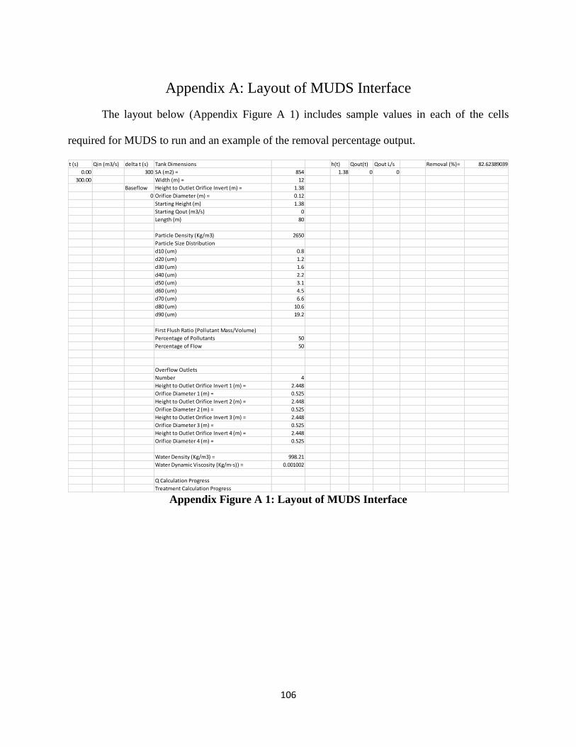
106
Appendix A: Layout of MUDS Interface
The layout below (Appendix Figure A 1) includes sample values in each of the cells
required for MUDS to run and an example of the removal percentage output.
Appendix Figure A 1: Layout of MUDS Interface
t (s) Qin (m3/s) delta t (s) Tank Dimensions h(t) Qout(t) Qout L/s Removal (%)= 82.62389039
0.00 300 SA (m2) = 854 1.38 0 0
300.00 Width (m) = 12
Baseflow Height to Outlet Orifice Invert (m) = 1.38
0 Orifice Diameter (m) = 0.12
Starting Height (m) 1.38
Starting Qout (m3/s) 0
Length (m) 80
Particle Density (Kg/m3) 2650
Particle Size Distribution
d10 (um) 0.8
d20 (um) 1.2
d30 (um) 1.6
d40 (um) 2.2
d50 (um) 3.1
d60 (um) 4.5
d70 (um) 6.6
d80 (um) 10.6
d90 (um) 19.2
First Flush Ratio (Pollutant Mass/Volume)
Percentage of Pollutants 50
Percentage of Flow 50
Overflow Outlets
Number 4
Height to Outlet Orifice Invert 1 (m) = 2.448
Orifice Diameter 1 (m) = 0.525
Height to Outlet Orifice Invert 2 (m) = 2.448
Orifice Diameter 2 (m) = 0.525
Height to Outlet Orifice Invert 3 (m) = 2.448
Orifice Diameter 3 (m) = 0.525
Height to Outlet Orifice Invert 4 (m) = 2.448
Orifice Diameter 4 (m) = 0.525
Water Density (Kg/m3) = 998.21
Water Dynamic Viscosity (Kg/m·s)) = 0.001002
Q Calculation Progress
Treatment Calculation Progress

107
Appendix B: Removal Percentage Calculation
As explained in Section 3.4.3, users are prompted to enter a particle size distribution
before running MUDS. These particle sizes represent thresholds, if a particle size settles to the
bottom of the USDC then a known percentage of TSS has been removed (e.g. if the d50 particle
has settled then 50% of TSS has been removed). MUDS tracks waves of particles as they
progress through the USDC, Appendix Figure B 1 represents how MUDS interprets the tracking
information calculated for each particle wave where hini is the initial height (m), and tf is the time
the particle wave exited the USDC (s). When visualizing the settling paths of these threshold
particle sizes, the settling paths can be interpreted as lines of removal (e.g. the d40 settling path
represents the 60% line of removal). The particles are divided into 10% segments by the lines of
removal.
Appendix Figure B 1: MUDS Settling Path Prediction
The settling velocity of a particle diameter can be determined using the following
equation:
𝑉𝑠 =
ℎ𝑖𝑛𝑖
𝑡𝑓 (B1)

108
The height of the particle at each point in time (hp(t)) can then be determined using this
simple equation of a line:
ℎ𝑝(𝑡) = −𝑉𝑠 ∗ 𝑡 + ℎ𝑖𝑛𝑖 (B2)
Rearranging for time yields equation B3:
𝑡 =
ℎ𝑝(𝑡) − ℎ𝑖𝑛𝑖
−𝑉𝑠=
ℎ𝑖𝑛𝑖 − ℎ𝑝(𝑡)
𝑉𝑠 (B3)
Not all threshold particle sizes reach the bottom of the USDC before reaching the outlet,
when this occurs there is a partial removal of the particles in the segment between the larger
threshold particle size that settled out and the one that did not. An average settling velocity for
the segment must be calculated to determine how much of the segment is removed. One of the
conditions to calculate this partial removal is that the difference between one line of removal
(e.g. 40%) to the time to finish must be equal to the difference between the next line (e.g. 50%)
at the same height. This is represented by the lines labeled a and b in Appendix Figure B 1, and
by the following equations:
𝑎 = 𝑏 (B4)
𝑡𝑓 − 𝑡𝑎 = 𝑡𝑏 − 𝑡𝑓 (B5)
Rearranging yields:
2𝑡𝑓 = 𝑡𝑏 + 𝑡𝑎 (B6)
This equation can be combined with the equation B3:
𝑡𝑎 =ℎ𝑖𝑛𝑖 − ℎ𝑝
𝑉𝑠𝑎 𝑡𝑏 =
ℎ𝑖𝑛𝑖 − ℎ𝑝
𝑉𝑠𝑏
𝑡𝑎 + 𝑡𝑏 =
ℎ𝑖𝑛𝑖 − ℎ𝑝
𝑉𝑠𝑎+
ℎ𝑖𝑛𝑖 − ℎ𝑝
𝑉𝑠𝑏 (B7)

109
𝑡𝑎 + 𝑡𝑏 =𝑉𝑠𝑎(ℎ𝑖𝑛𝑖 − ℎ𝑝) + 𝑉𝑠𝑏(ℎ𝑖𝑛𝑖 − ℎ𝑝)
𝑉𝑠𝑎 ∗ 𝑉𝑠𝑏
Where hp is the height at which a = b. Substituting using equation B6:
2𝑡𝑓 =
(ℎ𝑖𝑛𝑖 − ℎ𝑝)(𝑉𝑎 + 𝑉𝑏)
𝑉𝑠𝑎 ∗ 𝑉𝑠𝑏 (B8)
Finally, the height at which a = b can be calculated by rearranging:
ℎ𝑝 = ℎ𝑖𝑛𝑖 −
2𝑡𝑓 ∗ 𝑉𝑠𝑎 ∗ 𝑉𝑠𝑏
𝑉𝑠𝑎 + 𝑉𝑠𝑏 (B9)
The removal percentage of a segment attributed to the total removal of a wave is the ratio
of the settling velocity of the segment to the critical settling velocity for that wave times the
percentage that segment represents (10%)
𝑅𝐹𝑟𝑎𝑐𝑡𝑖𝑜𝑛 =
𝑉𝑠𝑒𝑔𝑚𝑒𝑛𝑡
𝑉𝑠𝑐∗ (𝑑𝑖𝑓𝑓 𝑖𝑛 %) (B10)
The settling velocity of the segment is calculated using equation B11:
𝑉𝑠𝑒𝑔𝑚𝑒𝑛𝑡 =
ℎ𝑖𝑛𝑖 − ℎ𝑝
𝑡𝑓 (B11)
Substituting with equation B9:
𝑉𝑠𝑒𝑔𝑚𝑒𝑛𝑡 =ℎ𝑖𝑛𝑖 − ℎ𝑖𝑛𝑖 +
2𝑡𝑓 ∗ 𝑉𝑎 ∗ 𝑉𝑏
𝑉𝑎 + 𝑉𝑏
𝑡𝑓
𝑉𝑠𝑒𝑔𝑚𝑒𝑛𝑡 =
2𝑉𝑎 ∗ 𝑉𝑏
𝑉𝑎 + 𝑉𝑏 (B12)
Making a final substitution yields the equation for the removal percentage of a segment
attributed to the total removal of a particle wave:
𝑅𝐹𝑟𝑎𝑐𝑡𝑖𝑜𝑛 =
2𝑉𝑎 ∗ 𝑉𝑏
(𝑉𝑎 + 𝑉𝑏) ∗ 𝑉𝑠𝑐∗ (𝑑𝑖𝑓𝑓 𝑖𝑛 %) (B13)
The critical settling velocity of the particle wave is calculated using equation B14:

110
𝑉𝑠𝑐 =
ℎ𝑖𝑛𝑖
𝑡𝑓 (B14)
There are special conditions where different removal percentage equations are applied.
These include: (1) removal of particles with settling velocity greater than the critical settling
velocity, this can have any value and is not limited to groupings of 10% (values can be 57%,
44%, etc.); (2) removal of particles left over in a ten percent group after calculating removal of
particles with Vs > Vsc (e.g. for 57% fully removed some fraction of the 3% remaining is
partially removed); (3) the fraction of particles removed with particle diameters smaller than the
d10; (4) when a particle group has a height at the outlet that is greater than the height at which it
entered the USDC, this can occur during high intensity and volume storm events cause the water
surface to rise quickly far above the outlet. The calculations for these situations are explained in
sections B.1 – B.4.
B.1 Particles with Vs > Vsc
MUDS begins by determining the smallest particle size that reached the bottom of the
USDC. Every particle larger than this has been fully removed, for example if a d50 is the smallest
particle size to reach the bottom of the USDC before the wave reaches the outlet then 50% of the
particles have been fully removed. The segment between the smallest to be removed and the next
smallest is divided by the critical settling velocity particle path. Therefore, a portion of the
segment is fully removed and a portion only has partial removal. The percentage of particles
fully removed between the smallest to be removed and the next smallest is calculated by linearly
interpolating between the time it takes the larger particle to reach the bottom, the time for a
particle settling at the critical settling velocity, and the time for the smaller particle to reach the
bottom.

111
𝑅𝐹𝑟𝑎𝑐𝑡𝑖𝑜𝑛 =
𝑡𝑓 − 𝑡𝑙𝑎𝑟𝑔𝑒𝑟
𝑡𝑠𝑚𝑎𝑙𝑙𝑒𝑟 − 𝑡𝑙𝑎𝑟𝑔𝑒𝑟∗ (10%) (B15)
Where RFraction is the removal percentage, tf is the time for the particle wave to reach the
outlet (s), tlarger is the time for the larger particle to reach the bottom of the USDC (s), and tsmaller
is the time for the smaller particle (s). The value for tlarger is tracked by MUDS, but tsmaller is
calculated using equation B16.
𝑡𝑠𝑚𝑎𝑙𝑙𝑒𝑟 =
ℎ𝑖𝑛𝑖
𝑉𝑠=
ℎ𝑖𝑛𝑖 ∗ 𝑡𝑓
ℎ𝑖𝑛𝑖 − ℎ𝑒𝑥𝑖𝑡 (B16)
Where hexit is the height at which the particle size exits the USDC. Appendix Figure B 2
shows how MUDS interprets these values.
Appendix Figure B 2: MUDs Interpretation of tlarger and tsmaller
B.2 Partial Removal of Particles after Fully Removed is Determined
The partial removal of the remaining portion of the segment that was not fully removed
in the calculation in Section B.1 is calculated using equation B13, but the value for Vsc is used in
place of Va. To determine what portion of the segment was not fully removed, another linear
interpolation is performed. The final equation for the removal of this segment of the particles is
shown in equation B17.

112
𝑅𝐹𝑟𝑎𝑐𝑡𝑖𝑜𝑛 =
2𝑉𝑠𝑐 ∗ 𝑉𝑏
(𝑉𝑠𝑐 + 𝑉𝑏) ∗ 𝑉𝑠𝑐∗
𝑡𝑠𝑚𝑎𝑙𝑙𝑒𝑟 − 𝑡𝑓
𝑡𝑠𝑚𝑎𝑙𝑙𝑒𝑟 − 𝑡𝑙𝑎𝑟𝑔𝑒𝑟∗ (10 %) (B17)
B.3 Removal of Particles between d10 and d0
It is assumed that the diameter of particles for the smallest 10 percent in the particle size
distribution can be linearly interpolated between the d10 and zero. Therefore, the average settling
velocity for those particles is the settling velocity of the d10 divided by two. The formula for the
removal of this section is presented in equation B18.
𝑅𝐹𝑟𝑎𝑐𝑡𝑖𝑜𝑛 =
h𝑖𝑛𝑖 − ℎ𝑒𝑥𝑖𝑡
2𝑡𝑓 ∗ 𝑉𝑠𝑐∗ (10 %) (B18)
B.4 Particle Exit Height is Greater than Entry Height
This situation can occur during high intensity and volume storm events that cause the
water level to rise quickly far above the outlet, and results in MUDS interpreting the particle
group as having a negative settling velocity. If a particle size has a negative settling velocity it is
assumed that none of the particles between that particle size and the next largest are removed by
the USDC. While this is not strictly true it is an assumption that gives a more conservative
answer for particle removal.
This circumstance can also effect the removal calculation in Section B.1, a particle size
may settle to the bottom but the next smallest may still exit at a height greater than the entry
height given the right conditions. If this occurs, it is assumed that there is no partial removal of
the 10% section and only the particles with diameters larger than the last to settle are fully
removed. For example, if the d50 is removed but the d40 exits at a height greater than the entry
height then only 50% of that wave is removed.

113
Appendix C: Hydrograph and Depth Figures of Storms used for
Validation and Calibration of the SWMM Model
September 2nd Hydrographs and Depth
0
2
4
6
8
10
12
140
60
120
180
240
300
360
0
21
00
42
00
63
00
84
00
10
50
0
12
60
0
14
70
0
16
80
0
18
90
0
21
00
0
23
10
0
25
20
0
27
30
0
29
40
0
31
50
0
33
60
0
35
70
0
37
80
0
39
90
0
42
00
0
44
10
0
46
20
0
48
30
0
50
40
0
52
50
0
54
60
0
56
70
0
58
80
0
60
90
0
Rai
nfa
ll (m
m/5
min
)
Flo
wra
te (
L/s)
Time (s)
NSE = 0.90
Rainfall Qin Modeled Qout Measured Qout Modeled
0
2
4
6
8
10
121.34
1.44
1.54
1.64
1.74
1.84
1.94
2.04
0
21
00
42
00
63
00
84
00
10
50
0
12
60
0
14
70
0
16
80
0
18
90
0
21
00
0
23
10
0
25
20
0
27
30
0
29
40
0
31
50
0
33
60
0
35
70
0
37
80
0
39
90
0
42
00
0
44
10
0
46
20
0
48
30
0
50
40
0
52
50
0
54
60
0
56
70
0
58
80
0
60
90
0
Rai
nfa
ll (m
m/5
min
)
Dep
th (
m)
Time (s)
NSE = 0.92
Rainfall Depth Monitored Depth Modeled

114
September 5th Hydrographs and Depth
0
2
4
6
8
10
12
140
60
120
180
240
300
360
420
480
26
40
0
28
80
0
31
20
0
33
60
0
36
00
0
38
40
0
40
80
0
43
20
0
45
60
0
48
00
0
50
40
0
52
80
0
55
20
0
57
60
0
60
00
0
62
40
0
64
80
0
67
20
0
69
60
0
72
00
0
74
40
0
76
80
0
79
20
0
81
60
0
84
00
0
86
40
0
88
80
0
91
20
0
93
60
0
96
00
0
Rai
nfa
ll (m
m/5
min
)
Flo
wra
te (
L/s)
Time (s)
NSE = 0.84
Rainfall Qin Modeled Qout Measured Qout Modeled
0
2
4
6
8
10
121.34
1.44
1.54
1.64
1.74
1.84
1.94
2.04
26
40
0
28
80
0
31
20
0
33
60
0
36
00
0
38
40
0
40
80
0
43
20
0
45
60
0
48
00
0
50
40
0
52
80
0
55
20
0
57
60
0
60
00
0
62
40
0
64
80
0
67
20
0
69
60
0
72
00
0
74
40
0
76
80
0
79
20
0
81
60
0
84
00
0
86
40
0
88
80
0
91
20
0
93
60
0
96
00
0
Rai
nfa
ll (m
m/5
min
)
Dep
th (
m)
Time (s)
NSE = 0.86
Rainfall Depth Measured Depth Modeled

115
September 10th Hydrographs and Depth
0
0.1
0.2
0.3
0.4
0.5
0.6
0.7
0.8
0.9
10
2
4
6
8
10
0
30
00
60
00
90
00
12
00
0
15
00
0
18
00
0
21
00
0
24
00
0
27
00
0
30
00
0
33
00
0
36
00
0
39
00
0
42
00
0
45
00
0
48
00
0
51
00
0
54
00
0
57
00
0
60
00
0
63
00
0
66
00
0
69
00
0
72
00
0
75
00
0
78
00
0
81
00
0
84
00
0
87
00
0
90
00
0
93
00
0
96
00
0
Rai
nfa
ll (m
m/5
min
)
Flo
wra
te (
L/s)
Time (s)
NSE = 0.45
Rainfall Qin Modeled Qout Measured Qout Modeled
0
0.1
0.2
0.3
0.4
0.5
0.6
0.7
0.8
0.9
11.4
1.405
1.41
1.415
1.42
1.425
0
30
00
60
00
90
00
12
00
0
15
00
0
18
00
0
21
00
0
24
00
0
27
00
0
30
00
0
33
00
0
36
00
0
39
00
0
42
00
0
45
00
0
48
00
0
51
00
0
54
00
0
57
00
0
60
00
0
63
00
0
66
00
0
69
00
0
72
00
0
75
00
0
78
00
0
81
00
0
84
00
0
87
00
0
90
00
0
93
00
0
96
00
0
Rai
nfa
ll (m
m/5
min
)
Dep
th (
m)
Time (s)
NSE = 0.53
Rainfall Depth Measured Depth Modeled

116
September 15th Hydrographs and Depth
0
0.2
0.4
0.6
0.8
1
1.2
1.4
1.6
1.8
20
2
4
6
8
10
0
30
00
60
00
90
00
12
00
0
15
00
0
18
00
0
21
00
0
24
00
0
27
00
0
30
00
0
33
00
0
36
00
0
39
00
0
42
00
0
45
00
0
48
00
0
51
00
0
54
00
0
57
00
0
60
00
0
63
00
0
66
00
0
69
00
0
72
00
0
75
00
0
78
00
0
81
00
0
84
00
0
87
00
0
90
00
0
93
00
0
96
00
0
Rai
nfa
ll (m
m/5
min
)
Flo
wra
te (
L/s)
Time (s)
NSE = 0.39
Rainfall Qin Modeled Qout Measured Qout Modeled
0
0.2
0.4
0.6
0.8
1
1.2
1.4
1.6
1.8
21.39
1.395
1.4
1.405
1.41
1.415
1.42
1.425
1.43
1.435
04
20
08
40
01
26
00
16
80
02
10
00
25
20
02
94
00
33
60
03
78
00
42
00
04
62
00
50
40
05
46
00
58
80
06
30
00
67
20
07
14
00
75
60
07
98
00
84
00
08
82
00
92
40
09
66
00
10
08
00
10
50
00
10
92
00
11
34
00
11
76
00
12
18
00
12
60
00
13
02
00
13
44
00
Rai
nfa
ll (m
m/5
min
)
Dep
th (
m)
Time (s)
NSE = 0.75
Rainfall Depth Measured Depth Modeled

117
September 22nd Hydrographs and Depth
0
1
2
3
4
5
6
7
8
9
100
50
100
150
200
250
300
350
0
30
00
60
00
90
00
12
00
0
15
00
0
18
00
0
21
00
0
24
00
0
27
00
0
30
00
0
33
00
0
36
00
0
39
00
0
42
00
0
45
00
0
48
00
0
51
00
0
54
00
0
57
00
0
60
00
0
63
00
0
66
00
0
69
00
0
72
00
0
75
00
0
78
00
0
81
00
0
84
00
0
87
00
0
90
00
0
93
00
0
96
00
0
Rai
nfa
ll (m
m/5
min
)
Flo
wra
te (
L/s)
Time (s)
NSE = 0.69
Rainfall Qin Modeled Qout Measured Qout Modeled
0
1
2
3
4
5
6
7
8
9
101.35
1.4
1.45
1.5
1.55
1.6
1.65
1.7
0
30
00
60
00
90
00
12
00
0
15
00
0
18
00
0
21
00
0
24
00
0
27
00
0
30
00
0
33
00
0
36
00
0
39
00
0
42
00
0
45
00
0
48
00
0
51
00
0
54
00
0
57
00
0
60
00
0
63
00
0
66
00
0
69
00
0
72
00
0
75
00
0
78
00
0
81
00
0
84
00
0
87
00
0
90
00
0
93
00
0
96
00
0
Rai
nfa
ll (m
m/5
min
)
Dep
th (
m)
Time (s)
NSE = 0.88
Rainfall Depth Measured Depth Modeled

118
October 3rd Hydrographs and Depth
0
0.2
0.4
0.6
0.8
1
1.2
1.4
1.6
1.8
20
2
4
6
8
10
12
14
16
18
20
0
30
00
60
00
90
00
12
00
0
15
00
0
18
00
0
21
00
0
24
00
0
27
00
0
30
00
0
33
00
0
36
00
0
39
00
0
42
00
0
45
00
0
48
00
0
51
00
0
54
00
0
57
00
0
60
00
0
63
00
0
66
00
0
69
00
0
72
00
0
75
00
0
78
00
0
81
00
0
84
00
0
87
00
0
90
00
0
93
00
0
96
00
0
Rai
nfa
ll (m
m/5
min
)
Flo
wra
te (
L/s)
Time (s)
NSE = 0.45
Rainfall Qin Modeled Qout Measured Qout Modeled
0
0.2
0.4
0.6
0.8
1
1.2
1.4
1.6
1.8
21.35
1.36
1.37
1.38
1.39
1.4
1.41
1.42
1.43
1.44
1.45
0
30
00
60
00
90
00
12
00
0
15
00
0
18
00
0
21
00
0
24
00
0
27
00
0
30
00
0
33
00
0
36
00
0
39
00
0
42
00
0
45
00
0
48
00
0
51
00
0
54
00
0
57
00
0
60
00
0
63
00
0
66
00
0
69
00
0
72
00
0
75
00
0
78
00
0
81
00
0
84
00
0
87
00
0
90
00
0
93
00
0
96
00
0
Rai
nfa
ll (m
m/5
min
)
Dep
th (
m)
Time (s)
NSE = 0.45
Rainfall Depth Measured Depth Modeled
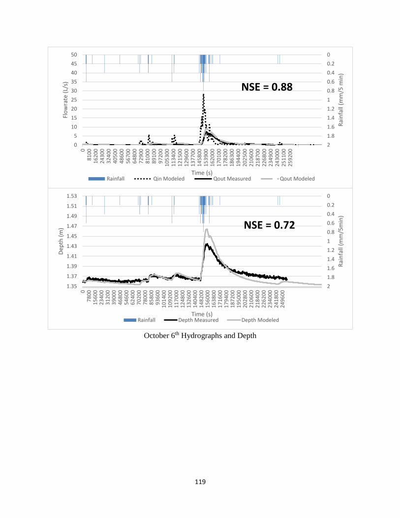
119
October 6th Hydrographs and Depth
0
0.2
0.4
0.6
0.8
1
1.2
1.4
1.6
1.8
20
5
10
15
20
25
30
35
40
45
50
08
10
01
62
00
24
30
03
24
00
40
50
04
86
00
56
70
06
48
00
72
90
08
10
00
89
10
09
72
00
10
53
00
11
34
00
12
15
00
12
96
00
13
77
00
14
58
00
15
39
00
16
20
00
17
01
00
17
82
00
18
63
00
19
44
00
20
25
00
21
06
00
21
87
00
22
68
00
23
49
00
24
30
00
25
11
00
25
92
00
Rai
nfa
ll (m
m/5
min
)
Flo
wra
te (
L/s)
Time (s)
NSE = 0.88
Rainfall Qin Modeled Qout Measured Qout Modeled
0
0.2
0.4
0.6
0.8
1
1.2
1.4
1.6
1.8
21.35
1.37
1.39
1.41
1.43
1.45
1.47
1.49
1.51
1.53
07
80
01
56
00
23
40
03
12
00
39
00
04
68
00
54
60
06
24
00
70
20
07
80
00
85
80
09
36
00
10
14
00
10
92
00
11
70
00
12
48
00
13
26
00
14
04
00
14
82
00
15
60
00
16
38
00
17
16
00
17
94
00
18
72
00
19
50
00
20
28
00
21
06
00
21
84
00
22
62
00
23
40
00
24
18
00
24
96
00
Rai
nfa
ll (m
m/5
min
)
Dep
th (
m)
Time (s)
NSE = 0.72
Rainfall Depth Measured Depth Modeled

120
October 15th Hydrographs and Depth
0
0.2
0.4
0.6
0.8
1
1.20
2
4
6
8
10
12
14
16
02
40
04
80
07
20
09
60
01
20
00
14
40
01
68
00
19
20
02
16
00
24
00
02
64
00
28
80
03
12
00
33
60
03
60
00
38
40
04
08
00
43
20
04
56
00
48
00
05
04
00
52
80
05
52
00
57
60
06
00
00
62
40
06
48
00
67
20
06
96
00
72
00
07
44
00
76
80
0
Rai
nfa
ll (m
m/5
min
)
Flo
wra
te (
L/s)
Time (s)
NSE = -1.96
Rainfall Qin Modeled Qout Measured Qout Modeled
0
0.2
0.4
0.6
0.8
1
1.21.35
1.37
1.39
1.41
1.43
1.45
0
24
00
48
00
72
00
96
00
12
00
0
14
40
01
68
00
19
20
02
16
00
24
00
02
64
00
28
80
03
12
00
33
60
0
36
00
0
38
40
04
08
00
43
20
0
45
60
04
80
00
50
40
05
28
00
55
20
05
76
00
60
00
06
24
00
64
80
06
72
00
69
60
0
72
00
0
74
40
07
68
00
Rai
nfa
ll (m
m/5
min
)
Dep
th (
m)
Time (s)
NSE = -0.17
Rainfall Depth Measured Depth Modeled

121
October 16th Hydrographs and Depth
0
1
2
3
4
5
60
20
40
60
80
100
120
140
160
180
0
21
00
42
00
63
00
84
00
10
50
0
12
60
0
14
70
0
16
80
0
18
90
0
21
00
0
23
10
0
25
20
0
27
30
0
29
40
0
31
50
0
33
60
0
35
70
0
37
80
0
39
90
0
42
00
0
44
10
0
46
20
0
48
30
0
50
40
0
52
50
0
54
60
0
56
70
0
58
80
0
60
90
0
63
00
0
65
10
0
Rai
nfa
ll (m
m/5
min
)
Flo
wra
te (
L/s)
Time (s)
NSE = 0.52
Rainfall Qin Modeled Qout Measured Qout Modeled
0
1
2
3
4
5
61.35
1.4
1.45
1.5
1.55
0
21
00
42
00
63
00
84
00
10
50
0
12
60
0
14
70
0
16
80
0
18
90
0
21
00
0
23
10
0
25
20
0
27
30
0
29
40
0
31
50
0
33
60
0
35
70
0
37
80
0
39
90
0
42
00
0
44
10
0
46
20
0
48
30
0
50
40
0
52
50
0
54
60
0
56
70
0
58
80
0
60
90
0
63
00
0
65
10
0
Rai
nfa
ll (m
m/5
min
)
Dep
th (
m)
Time (s)
NSE = 0.36
Rainfall Depth Measured Depth Modeled
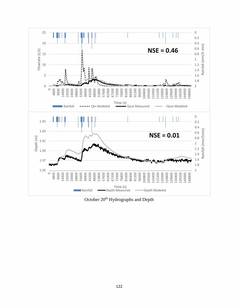
122
October 20th Hydrographs and Depth
0
0.2
0.4
0.6
0.8
1
1.2
1.4
1.6
1.8
20
5
10
15
20
25
0
48
00
96
00
14
40
0
19
20
0
24
00
0
28
80
0
33
60
0
38
40
0
43
20
0
48
00
0
52
80
0
57
60
0
62
40
0
67
20
0
72
00
0
76
80
0
81
60
0
86
40
0
91
20
0
96
00
0
10
08
00
10
56
00
11
04
00
11
52
00
12
00
00
12
48
00
12
96
00
13
44
00
13
92
00
14
40
00
14
88
00
Rai
nfa
ll (m
m/5
min
)
Flo
wra
te (
L/s)
Time (s)
NSE = 0.46
Rainfall Qin Modeled Qout Measured Qout Modeled
0
0.2
0.4
0.6
0.8
1
1.2
1.4
1.6
1.8
21.35
1.37
1.39
1.41
1.43
1.45
0
48
00
96
00
14
40
0
19
20
0
24
00
0
28
80
0
33
60
0
38
40
0
43
20
0
48
00
0
52
80
0
57
60
0
62
40
0
67
20
0
72
00
0
76
80
0
81
60
0
86
40
0
91
20
0
96
00
0
10
08
00
10
56
00
11
04
00
11
52
00
12
00
00
12
48
00
12
96
00
13
44
00
13
92
00
14
40
00
14
88
00
Rai
nfa
ll (m
m/5
min
)
Dep
th (
m)
Time (s)
NSE = 0.01
Rainfall Depth Measured Depth Modeled

123
November 6th Hydrographs and Depth
0
0.2
0.4
0.6
0.8
1
1.2
1.4
1.6
1.8
20
2
4
6
8
10
12
14
0
27
00
54
00
81
00
10
80
0
13
50
0
16
20
0
18
90
0
21
60
0
24
30
0
27
00
0
29
70
0
32
40
0
35
10
0
37
80
0
40
50
0
43
20
0
45
90
0
48
60
0
51
30
0
54
00
0
56
70
0
59
40
0
62
10
0
64
80
0
67
50
0
70
20
0
72
90
0
75
60
0
78
30
0
81
00
0
Rai
nfa
ll (m
m/5
min
)
Flo
wra
te (
L/s)
Time (s)
NSE = 0.72
Rainfall Qin Modeled Qout Measured Qout Modeled
0
0.1
0.2
0.3
0.4
0.5
0.6
0.7
0.8
0.9
11.35
1.36
1.37
1.38
1.39
1.4
1.41
1.42
0
27
00
54
00
81
00
10
80
0
13
50
0
16
20
0
18
90
0
21
60
0
24
30
0
27
00
0
29
70
0
32
40
0
35
10
0
37
80
0
40
50
0
43
20
0
45
90
0
48
60
0
51
30
0
54
00
0
56
70
0
59
40
0
62
10
0
64
80
0
67
50
0
70
20
0
72
90
0
75
60
0
78
30
0
81
00
0
Rai
nfa
ll (m
m/5
min
)
Dep
th (
m)
Time (s)
NSE = 0.21
Rainfall Depth Measured Depth Modeled

124
November 17th Hydrographs and Depth
0
0.2
0.4
0.6
0.8
1
1.2
1.4
1.6
1.8
20
2
4
6
8
10
12
14
0
21
00
42
00
63
00
84
00
10
50
0
12
60
0
14
70
0
16
80
0
18
90
0
21
00
0
23
10
0
25
20
0
27
30
0
29
40
0
31
50
0
33
60
0
35
70
0
37
80
0
39
90
0
42
00
0
44
10
0
46
20
0
48
30
0
50
40
0
52
50
0
54
60
0
56
70
0
58
80
0
60
90
0
63
00
0
65
10
0
Rai
nfa
ll (m
m/5
min
)
Flo
wra
te (
L/s)
Time (s)
NSE = -0.32
Rainfall Qin Modeled Qout Measured Qout Modeled
0
0.1
0.2
0.3
0.4
0.5
0.6
0.7
0.8
0.9
11.35
1.37
1.39
1.41
1.43
1.45
0
21
00
42
00
63
00
84
00
10
50
0
12
60
0
14
70
0
16
80
0
18
90
0
21
00
0
23
10
0
25
20
0
27
30
0
29
40
0
31
50
0
33
60
0
35
70
0
37
80
0
39
90
0
42
00
0
44
10
0
46
20
0
48
30
0
50
40
0
52
50
0
54
60
0
56
70
0
58
80
0
60
90
0
63
00
0
65
10
0
Rai
nfa
ll (m
m/5
min
)
Dep
th (
m)
Time (s)
NSE = -4.3
Rainfall Depth Measured Depth Modeled
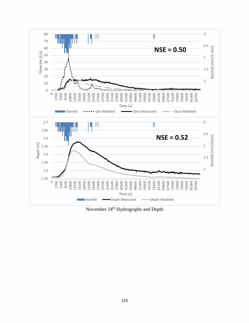
125
November 24th Hydrographs and Depth
0
0.5
1
1.5
2
0
10
20
30
40
50
60
70
80
0
27
00
54
00
81
00
10
80
0
13
50
0
16
20
0
18
90
0
21
60
0
24
30
0
27
00
0
29
70
0
32
40
0
35
10
0
37
80
0
40
50
0
43
20
0
45
90
0
48
60
0
51
30
0
54
00
0
56
70
0
59
40
0
62
10
0
64
80
0
67
50
0
70
20
0
72
90
0
75
60
0
78
30
0
81
00
0
83
70
0
Rai
nfa
ll (m
m/5
min
)
Flo
wra
te (
L/s)
Time (s)
NSE = 0.50
Rainfall Qin Modeled Qout Measured Qout Modeled
0
0.5
1
1.5
2
1.35
1.4
1.45
1.5
1.55
1.6
1.65
1.7
0
27
00
54
00
81
00
10
80
0
13
50
0
16
20
0
18
90
0
21
60
0
24
30
0
27
00
0
29
70
0
32
40
0
35
10
0
37
80
0
40
50
0
43
20
0
45
90
0
48
60
0
51
30
0
54
00
0
56
70
0
59
40
0
62
10
0
64
80
0
67
50
0
70
20
0
72
90
0
75
60
0
78
30
0
81
00
0
83
70
0
Rai
nfa
ll (m
m/5
min
)
Dep
th (
m)
Time (s)
NSE = 0.52
Rainfall Depth Measured Depth Modeled