a technique for mapping urban areas and … · iii a technique for mapping urban areas and change...
TRANSCRIPT

A TECHNIQUE FOR MAPPING URBAN AREAS AND CHANGE USING
INTEGRATED REMOTE SENSING AND DASYMETRIC POPULATION MAPPING
METHODS
A THESIS PRESENTED TO
THE DEPARTMENT OF GEOLOGY AND GEOGRAPHY
IN CANDIDACY FOR THE DEGREE OF
MASTER OF SCIENCE
By
STEPHEN W. SANFORD
NORTHWEST MISSOURI STATE UNIVERSITY
MARYVILLE, MO
OCTOBER, 2011
MAPPING URBAN AREAS
A Technique for Mapping Urban Areas and Change Using Integrated
Remote Sensing and Dasymetric Population Mapping Methods
Stephen Sanford
Northwest Missouri State University
THESIS APPROVED
________________________________________________________________________
Thesis Advisor, Dr. Yi-Hwa Wu Date
________________________________________________________________________
Dr. Ming-Chih Hung Date
________________________________________________________________________
Dr. Matthew R. Engel Date
________________________________________________________________________
Dean of the Graduate School Date
iii
A Technique for Mapping Urban Areas and Change Using Integrated
Remote Sensing and Dasymetric Population Mapping Methods
ABSTRACT
In recent decades, mapping of urban areas and growth has been a vital tool in facing
many environmental challenges. In spite of this, a standard operational definition of
―urban‖ is lacking in the GIS and remote sensing literature. Definitions tend to vary
depending upon the specific application for which information is required. The purpose
of this study was to develop a pixel-level dasymetric technique for mapping urban areas
and their change over time utilizing two fundamental criteria for an urban environment:
urban population density and the presence of impervious surface. These sources were
used complementarily, as remote sensing methods for urban detection neglect well-
vegetated areas with urban population density, while the use of population data alone
neglects many commercial and industrial areas, blighted or abandoned urban areas, and
other developed areas where no one resides. Integrating satellite-derived land-cover data
with dasymetrically-derived population distribution data, urban areas and change of the
St. Louis Metropolitan Statistical Area (MSA) from 1990 to 2000 are mapped and
analyzed. It was shown that the use of one data source alone detects only roughly 73% of
the total urban area, which stresses the necessity of using both data sources for urban area
delineation. An accuracy assessment was performed on the classification. Both the 1989
and 2000 classifications achieved 89.6% accuracy. The dasymetric results were
compared with the original 1990 and 2000 census block population data and covered
82.5% and 84.0% of the same area, respectively.

iv
TABLE OF CONTENTS
Abstract iii
Table of Contents iv
List of Figures v
List of Tables vii
Chapter 1: Introduction 8
1.1 Research Objective 10
1.2 Justification 10
1.3 Definition of Dasymetric Mapping 10
1.4 Study Area 11
1.4.1 The Fringe Growth and Central City Decline of the St. Louis Area 12
Chapter 2: Literature Review 14
2.1 Remote Sensing Techniques in Mapping Urban Areas 14
2.2 Methods for Estimation of Population Using GIS and Remote Sensing 16
2.2.1 Statistical Modeling of Population 17
2.2.2 Dasymetric Mapping of Population 20
Chapter 3: Methodology 22
3.1 Data Sources and Analysis Extent 23
3.2 Classification 24
3.3 Dasymetric Mapping 27
3.4 Integration 36
Chapter 4: Analysis Results 39
4.1 Where was the Change and Why? 39
4.2 Density Change in and near the City 48
4.3 Methodology Validation 49
4.4 Accuracy Assessment 53
Chapter 5: Conclusion 58
5.1 Analysis Problems and Limitations 59
5.2 Future Development 60
References 62

v
LIST OF FIGURES
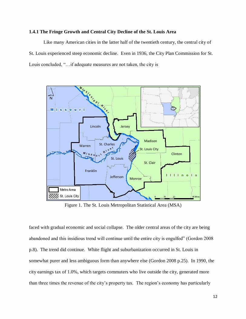
Figure 1. The St. Louis Metropolitan Statistical Area (MSA) 12
Figure 2. Research framework 22
Figure 3. Analysis extent 24
Figure 4. Classification of 1989 TM imagery 26
Figure 5. Classification of 2000 ETM+ imagery 26
Figure 6. New impervious surface 1990 – 2000 27
Figure 7. Urban population density in 1990 34
Figure 8. Urban population density in 2000 34
Figure 9. Change in urban population density 1990 – 2000 35
Figure 10. Comprehensive urban areas 1990 37
Figure 11. Comprehensive urban areas 2000 37
Figure 12. Comprehensive urban areas change 1990 – 2000 38
Figure 13. Non-urban to urban conversion distribution 41
Figure 14. Example areas converted to urban by land-cover 41
Figure 15. Example areas converted to urban by population (Missouri) 43
Figure 16. Example areas converted to urban by population (Illinois) 43
Figure 17. Urban to non-urban conversion distribution 44
Figure 18. Example areas converted to non-urban by population 46
Figure 19. Areas near Lambert Airport falling below urban population 46
density 1990 – 2000
Figure 20. Division of blocks between decennial censuses causing 47
misleading results
Figure 21. Population density change in and near St. Louis city 1990 – 2000 49
vi
Figure 22. Urban population density overlaying urban land-cover 1990 50
Figure 23. Urban land-cover overlaying urban population density 1990 51
Figure 24. Urban population density overlaying urban land-cover 2000 51
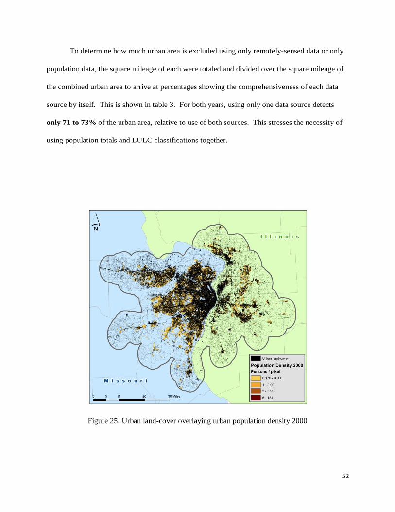
Figure 25. Urban land-cover overlaying urban population density 2000 52
Figure 26. Locations of DOQs for 1990 classification accuracy assessment 55
Figure 27. Locations of DOQs for 2000 classification accuracy assessment 56
vii
LIST OF TABLES
Table 1. RDensity values 31
Table 2. Distribution of urban/non-urban conversion 40
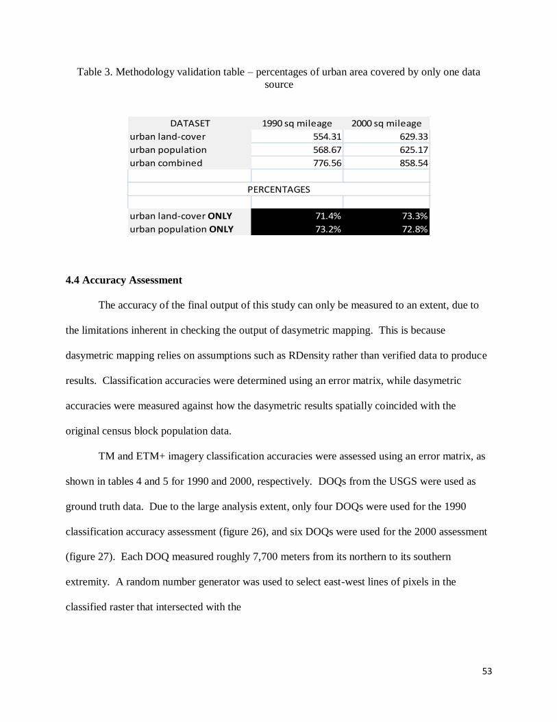
Table 3. Methodology validation table – percentages of urban area 53
covered by only one data source
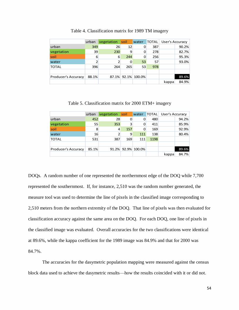
Table 4. Classification matrix for 1989 TM imagery 54
Table 5. Classification matrix for 2000 ETM+ imagery 54
Table 6. Accuracy assessment for dasymetric urban population mapping 57
8
CHAPTER 1: INTRODUCTION
In recent decades, mapping of urban areas and growth has been a vital tool in facing
many environmental challenges. Dynamic land-use/land-cover (LULC) change has implications
for sustainability of development, environmental health, global climate change, ecosystems, and
food production. Increasing and migrating population has ramifications for consumption of
natural resources, local socioeconomics, and commercial and industrial activity. Yet in spite of
these associations, a standard operational definition of ―urban‖ is lacking in the GIS and remote
sensing literature. The purpose of this research was to develop a dasymetric technique for
mapping urban areas and their change over time utilizing two fundamental criteria for an urban
environment: urban population density and the presence of impervious surface. It is shown that
use of these data sources together yields much more comprehensive results than when either is
used alone.
Many remote sensing studies treat ―urban‖ as equivalent to ―urban land-cover‖ or focus
on urban phenomena related merely to impervious surface (Grey et al. 2003, Herold et al. 2003a,
Li and Yeh 1998, Seto and Liu 2003, Wilson et al. 2003). In fact, one of the main difficulties in
urban analysis is that there is little consensus as to what constitutes urban land, and definitions
vary depending upon the specific application of the study (Weber 2001). This is apparent
especially in land-cover change detection studies, where ―urban boundaries‖ are assumed to shift
according to land-cover conversion to impervious surface, a conception that is unidimensional
and behavioristic. It does not take into account other important, on-the-ground variables, such as
the spatial distribution and density of population. Remote sensing methods for urban detection
show only areas of increased impervious surface and artificial structures, which neglect well-
9
vegetated areas with urban population density. Classification algorithms used in a plethora of
studies categorize areas of vegetation in urban environments as non-urban because the spectral
signatures of those areas are very similar if not identical to those of rural vegetated areas (Haack
et al. 2000, Masek et al. 2000, Ryznar and Wagner 2001, Gluch 2002, Haack et al. 2002, Grey et
al. 2003, Herold et al. 2003a and 2003b, Hodgson et al. 2003, Qiu et al. 2003, Seto and Liu
2003, Thomas et al. 2003, Weber and Puissant 2003, Yang et al. 2003, Zha et al. 2003, Alberti et
al. 2004, Huang et al. 2007). In other words, these studies fail to delineate an entire urban area
by limiting their criteria for an urban environment to the existence of impervious surface. At the
same time, urban population distribution and densities may or may not coincide with significant
areas of human-made structures. Census data neglect many commercial and industrial areas,
blighted and abandoned urban areas, and other developed areas where few or no people reside
such as power plants and isolated industrial facilities. Examples of these areas in this study area
include Earth City Industrial Park, large sections of East St. Louis, Illinois, and the Wood River
oil refinery in Roxana, Illinois.
Schneider et al. (1377) showed that integration of gridded population data with Moderate
Resolution Imaging Spectroradiometer (MODIS) and the Defense Meteorological Satellite
Program’s Operational Linescan System (DMSP/OLS) nighttime lights data ―improves urban
classification by resolving confusion between urban and other classes that occurs when any one
of the data sets is used by itself.‖ This study took their integrative methodology as a key
guideline and presents a technique for mapping urban environments and their change over time.
Integrating satellite-derived land-cover data with dasymetric population density and distribution
data, urban areas and change of the St. Louis area from 1990 to 2000 were mapped and analyzed.
10
1.1 Research Objective
The objective of this study was to develop and validate a technique for mapping urban
areas and change that integrates data on both urban structure development and population
density. The key idea was to demonstrate that use of both sources produces more accurate,
comprehensive results than either source would alone. A ―Methodology validation table‖ was
provided to prove statistically that significant areas of urban land are neglected when one or the
other input data sources is used alone.
1.2 Justification
Justification for this study is twofold. First, as stated, accurate and comprehensive
mapping of urban areas and change is crucial for, among other things, sustainable and
environmentally-conscious development and natural resource management. Second, there is
need to demonstrate the impact on urban area and change studies of not complementing
remotely-sensed data with on-the-ground data such as population data. Though census data in
the United States are collected only decennially and are generalized over zones, population data
are a vital data source for analysis of the spatial extent of an urban area. Furthermore, extraction
of population data from such generalized zones is possible by certain assumptions in the use of
dasymetric mapping, which, in this study, is used to project population figures from the census
block level to the pixel resolution of the remotely-sensed data.
1.3 Definition of Dasymetric Mapping
Dasymetric mapping uses secondary or multiple data sources to infer information from a
primary data source, frequently to reproject the primary data at a finer scale or in more detailed
11
manner. A typical example is the use of land-cover data to infer where population likely resides
within a general population zone, such as a census block, block group, or tract. Land-cover
categories typically coincident with residences—e.g., impervious surface as opposed to wetlands
or forest—are assumed to be areas where much of the population of the zone reside. The two
data sources—the land-cover data and the population zone data—are then combined in a
complex, mathematical way to produce more precise estimations as to where population resides.
It is important to note that dasymetric mapping works from assumptions rather than verified
information because the latter is lacking. The assumption in the example above is that
population likely resides in areas of impervious surface land-cover. The verified information
that is lacking is population data that are finer or more detailed than that at the general
population zone.
1.4 Study Area
As of 2000, the St. Louis Metropolitan Statistical Area (MSA) (figure 1) had a population
of 2,603,607, up from 2,492,525 in 1990, making it the 18th largest metro area in the US in 2000
(US Census Bureau Population Division 2011a). The City of St. Louis, with a 2000 population
of 348,189, lies just south of the confluence of the Mississippi and Missouri Rivers, on the
border of Missouri and Illinois (US Census Bureau Population 2011b). As of 2000, the
metropolitan area consisted of 12 counties: on the Missouri side, Franklin, Jefferson, Lincoln, St.
Charles, St. Louis City, St. Louis County, and Warren; on the Illinois side, Clinton, Jersey,
Madison, Monroe, and St. Clair (US Census Bureau Geography Division 2011).
12
1.4.1 The Fringe Growth and Central City Decline of the St. Louis Area
Like many American cities in the latter half of the twentieth century, the central city of
St. Louis experienced steep economic decline. Even in 1936, the City Plan Commission for St.
Louis concluded, ―…if adequate measures are not taken, the city is
Figure 1. The St. Louis Metropolitan Statistical Area (MSA)
faced with gradual economic and social collapse. The older central areas of the city are being
abandoned and this insidious trend will continue until the entire city is engulfed‖ (Gordon 2008
p.8). The trend did continue. White flight and suburbanization occurred in St. Louis in
somewhat purer and less ambiguous form than anywhere else (Gordon 2008 p.25). In 1990, the
city earnings tax of 1.0%, which targets commuters who live outside the city, generated more
than three times the revenue of the city’s property tax. The region’s economy has particularly
St. Charles
Lincoln
Warren
Jefferson
St. Louis
Franklin
Jersey
Madison
Clinton
St. Clair
Monroe
St. Louis City
13
suffered in recent years, as a host of corporate mergers and buyouts has signified St. Louis’
declining role in the national and international economy, sending more money out of the area
than would have been kept in: McDonnell-Douglas with Boeing, Ralston Purina with Nestle,
Trans World Airlines with American Airlines, Famous Barr with Macy’s, Mallinckrodt with
Tyco, Jones Pharma with King Pharmaceuticals, Monsanto with Pharmacia/Upjohn, and most
recently in 2008, Anheuser-Busch with InBev.
Ironically, however, it is this decline, both economic and in general living conditions and
quality of life, along with the typical, predictable growth on the urban fringes of any large metro,
that makes St. Louis an apt study area for this project. It was chosen because:
(1) Much of the area’s population resides in suburbs and exurbs rather than the central
city. According to the 2000 Census, only 12.9% of the metro lived in the central city
of St. Louis, as compared to Indianapolis’ 51%, Chicago and Kansas City’s 32%,
Detroit’s 21%, and Cincinnati’s 16.5%.
(2) Many of those suburbs are well-vegetated.
(3) Areas of decline and physical ruin are contrasted with areas of rapid development.
Traits two and three particularly make this urban area vulnerable to the pitfalls of utilizing only
remotely-sensed data, because vegetation can cover up impervious surface, and studies have
shown it is difficult to accurately measure population growth and exodus by satellite imagery
(Iisaka and Hegedus 1982; Langford et al. 1991; Lo 1995; Webster 1996; Harvey 2002a &
2002b; Li and Weng 2005; Liu et al. 2006; Wu et al. 2006).

14
CHAPTER 2: LITERATURE REVIEW
2.1 Remote Sensing Techniques in Mapping Urban Areas
In the past two decades, a variety of methods have been used to map urban areas. A
number of studies have used nighttime lights imagery from the DMSP (Henderson et al. 2003,
Imhoff et al. 1997, Sutton 1998 & 2003, and Lo 2001 & 2002). The value of this data source lies
in the idea that lighting is coincident with urban areas. However, there are a number of
drawbacks to it. First, spatial resolution is very low at 2.7 km. Second, the data has a blooming
effect which overestimates city size even when a fixed radiance value is determined from
comparison with, e.g., census urbanized area data. The fixed radiance value is intended to be a
standard threshold to determine where the urbanized/less-urbanized boundary is for all cities in a
global region, such as North America. Thus the nighttime lights data not only exaggerate the
area they supposedly represent but also cannot be used alone to accurately demarcate boundaries
(Imhoff et al. 1997, Schneider et al. 2003). Third, Schneider et al. (2003, p.1378) pointed out
that DMSP/OLS data ―do not necessarily represent the built environment or settlement patterns.
In particular, brightly lit agricultural areas and non-urban light sources such as gas flares and
fires are captured in these datasets.‖
Another method arising in recent years is the use of Radio Detection and Ranging
(RADAR) and Light Detection and Ranging (LiDAR) data to map urban morphology (Haack et
al. 2000 & 2002, Grey and Luckman 2003, Hodgson et al. 2003, Huang et al. 2007). Grey and
Luckman (2003) used phase coherence between pairs of Synthetic Aperture Radar (SAR) images
to determine urban areas. Whereas vegetation grows and withers throughout the seasons, urban
structures do not. They are coherent, i.e. constant, between two images. That is, impervious
surface appears on RADAR the same in the winter as it does in the summer. The single- or
15
double-bounce backscattering of man-made structures also makes urban areas detectable. In
other studies, RADAR or LiDAR has been used in combination with optical satellite data.
Huang et al. (2007) found that fusion of Landsat and Radarsat data improved classification
accuracy by 10 percent. Hodgson et al. (2003) used LiDAR in combination with
orthophotography to produce a regression line slope for detecting impervious surfaces showing a
near-perfect relationship between observed and predicted imperviousness (y = 1.016). Germaine
and Hung (2011) designed Knowledge Based Expert System (KBES) rules from LiDAR data to
increase the accuracy of an Iterative Self-Organizing Data Analysis Techniques (ISODATA)
classification from 91% with a kappa of 82.0% to 94% and a kappa of 87.9%. Despite these
boosts in classification accuracy, however, as a stand-alone remote sensing method for urban
delineation, RADAR and LiDAR inherit the drawbacks mentioned in the introduction of optical
remote sensing methods: they may not detect well-vegetated areas of urban population density.
Predictably, the existing literature for the use of daytime optical satellite imagery is
substantial (Li and Yeh 1998, Masek et al. 2000, Gluch 2002, Hung and Ridd 2002, Grey et al.
2003, Herold et al. 2003a & 2003b, Seto and Liu 2003, Thomas et al. 2003, Weber and Puissant
2003, Yang et al. 2003, Zha et al. 2003, Wilson et al. 2003, Alberti et al. 2004). Li and Yeh
(1998) classified urban land-cover from Thematic Mapper (TM) imagery to monitor urban
expansion in the Pearl River Delta, China. Others have taken on more refined methodologies,
such as altering classifiers for higher classification accuracy. Seto and Liu (2003) used an
artificial neural network, rather than a more conventional technique like the Bayesian Maximum-
Likelihood Classifier (MLC). Others implemented a Normalized Difference Built-up Index
(NDBI) with accuracy of 92.6% for automated mapping of urban areas (Zha et al. 2003). Hung
and Ridd (2002) developed a sub-pixel classification approach that iteratively adjusts
16
percentages of land-cover according to a linear mixture model. This allowed for classification of
land-cover by percentage of land-cover in a pixel. In another study, the use of spatial metrics
and image texture proved valuable in extracting urban land use from images (Herold et al. 2003a
& 2003b).
A handful of studies have used GIS and remote sensing data and methods together to
delineate an urban area (Chen et al. 2000, Ryznar and Wagner 2001, Abed and Kaysi 2003, Qiu
et al. 2003, Schneider et al. 2003). Abed and Kaysi (2003) used intensity of economic activity
as a factor, defined as number of employees in a statistical zone divided by housing units,
divided by surface area of the zone. These data were utilized along with density of the built-up
area of Beirut and fuzzy classification of SPOT pixels for relative variety or richness of land use.
Ryznar and Wagner (2001) used demographic data from the 1970, 1980, and 1990 censuses to
correlate with the output from Normalized Difference Vegetation Index (NDVI) images of inner
city and suburban Detroit. Results showed strong negative correlation between population and
vegetation growth in the inner city, verifying abandonment and overgrowth of vegetation around
and on urban structures. They also showed strong positive correlation for the suburbs, indicating
land-cover conversion from agricultural areas to residential lawns and vegetated areas. To sum,
these studies showed that the integration of population data enhances accuracy in mapping urban
areas and growth.
2.2 Methods for Estimation of Population Using GIS and Remote Sensing
Some studies have focused on estimation of population or population density rather than
on delineation of urban boundaries. The methods used can be grouped into two categories:
statistical modeling and areal interpolation. Statistical modeling infers relationships between
17
population and other variables to estimate the population for a given area. Areal interpolation
involves transforming data from one set of spatial units to another. Dasymetric mapping is a
form of areal interpolation.
2.2.1 Statistical Modeling of Population
Five types of approaches have been developed within the statistical modeling method,
and they are based on the relationship between population and 1) urban areas, 2) land use, 3)
dwelling units, 4) image pixel characteristics, and 5) other physical or socioeconomic
characteristics.
Urban nighttime lights have been used not just to delineate urban boundaries but also to
estimate population. Prosperie and Eyton (2000) found a correlation coefficient of R2
= 0.974
between light volumes and populations of 254 Texas counties using DMSP imagery. Also, Lo
(2002) determined a correlation coefficient of 0.91 between the light volumes of 35 Chinese
cities and their non-agricultural populations. Generally, however, correlating different types of
land use with population produces better results than use of DMSP data. Weber (1994) classified
land use from SPOT HRV XS images for Strasbourg, France and performed a regression
analysis of population counts and land use areas obtaining a correlation coefficient of R2 = 0.91.
Applying the regression model, he estimated the total population of the city to be 7.91% below
the actual census population. In a similar study, Lo (2003) used a logarithmic transformed
allometric growth model and estimated population in Atlanta with an overall underestimate of
8.07%.
Furthermore, population has been determined by multiplying the total number of
dwelling units with the number of persons normally living in a dwelling unit. Maantay et al.

18
(2007) used cadastral data of New York City to estimate population achieving an R2 value of
0.99. Lwin and Murayama (2009) used areametric and volumetric methods to estimate
population within buildings. The areametric method does not require data on number of building
floors and was suitable for low-rise buildings in rural areas, while the volumetric method does
require data on number of floors and was suitable for high-rise buildings, especially in
downtown areas. A regression analysis was performed comparing estimated population to actual
population with an R2 = 0.80 for the areametric method and R
2 = 0.95 for the volumetric method.
Wu et al. (2006) developed a deterministic model for sub-block-level population estimation
using GIS data on building volumes and housing statistics derived from the census. Assessment
of the results showed that the smaller the area, the higher the error, with an average percent error
of just 0.11 percent for areas equal in size to that from which they were disaggregated (the block
level), 15 percent for areas half of a block in area, and 35 percent for areas five percent of a
block area.
A number of studies have used image pixel characteristics to estimate population density.
Aggregated predictor variables in remote sensing have included mean reflectance of individual
spectral bands (Iisaka and Hegedus 1982; Lo 1995; Harvey 2002a & 2002b), numbers of pixels
in various land use categories (Langford et al. 1991; Lo 1995), measures of variability and image
texture (Webster 1996; Harvey 2002a and 2002b), and various band-to-band ratios and other
mathematical transformations of the multispectral data (Harvey 2002a and 2002b). These
studies demonstrated a significant correlation between population and remote sensing indicators,
with values for R2 in the 80 to 90 percent range. Harvey (2002b) developed an expectation-
maximization algorithm to iteratively regress pixel population on spectral indicators and re-
estimate pixel population with 16 percent error for one study area and 21 percent for another.
19
Wu et al. (2006) used image texture statistics of semi-variance to estimate population for
residential land use in the Austin, Texas area with an overall mean absolute relative error
(MARE) of 12 percent. Others encourage using image pixel characteristics with census data to
achieve higher accuracy. Liu et al. (2006) found that use of a gray-level co-occurrence matrix
(GLCM), semi-variance, and spatial metrics yielded varying correlations with population
density, the highest being the spatial metrics method. They concluded that the correlation
between image texture and population was not strong enough to predict residential population,
however texture does provide a base to refine census data. Also, Li and Weng (2005) used
textures, temperature, and spectral signatures to boost an estimation of the population of
Indianapolis in 2000 to 96.8 percent accuracy. In a review of the field, Wu et al. (2006 p.69)
concluded that ―more studies are needed before remote sensing can be applied to population
estimation on an operational basis.‖
Finally, numerous other physical and socioeconomic variables can also be incorporated
for population estimation. Liu and Clarke (2002) correlated population in urban areas with
distance from the Central Business District (CBD), accessibility to transportation systems, slope,
and the time when the residential community was first built. Qiu et al. (2003) modeled
population growth in the Dallas-Ft.Worth Metroplex from 1990 to 2000 using GIS-derived road
development measurements. Also, the Landscan Global Population Project uses light volume
from nighttime imagery, land cover, and other information about demography, topography, and
transportation networks to estimate population at a 30 x 30 second resolution (Dobson et al.
2000).
20
2.2.2 Dasymetric Mapping of Population
Despite the prolific use of statistical modeling methods, ―the dasymetric method is
commonly regarded as a more accurate approach, provided that the used ancillary information
gives a truthful description of where people actually live‖ (Wu et al. 2006 p.69). The literature
on dasymetric mapping of population, however, is comparatively limited. The reason for this,
conjectured among several authors, is the inherent difficulty and lack of standard methods in
producing dasymetric versus choropleth maps (Maantay et al. 2007). As stated, dasymetric
mapping uses secondary or multiple data sources to infer information from a primary data
source, frequently to reproject the primary data at a finer scale or in more detailed manner—a
conjunction of data sources in a complex way. Despite the rigors involved with dasymetric
mapping, there is some valuable research upon which the methodology for this study builds.
Maantay et al. (2007) proposed a Cadastral-based Expert Dasymetric System (CEDS),
whereby Census tract population data is disaggregated to parcels according to number of
residential units and residential areas of parcels. The authors claimed dasymetric studies using
land-use/land-cover (LULC) data are highly inaccurate relative to their own, however, their
technique has several drawbacks. First, for areas ranging from multiple counties to the size of a
metropolis or region, the residential unit data would have to be collected from multiple
governmental sources, with perhaps different levels of data completion, and merged seamlessly,
which could take considerably more time and manual work than acquiring remotely-sensed
imagery. Second, using their methodology, data at a resolution finer than TM pixels would
likely only be gained in high-density urban environments (such as their study area, New York
City) and would not be useful for broader study areas including suburbs and exurbs. Parcels
vary in size, while pixels are a constant area. Also, parcels are an arbitrary boundary and are

21
subject to all Modifiable Area Unit Problem (MAUP) issues. This is a significant problem for all
areas not of high-density urban LULC because generalization would result within parcels, likely
more than within moderate- or high-resolution pixels.
In contrast to parcels, Holloway et al. (1999) used LULC data as the ancillary data source
for producing dasymetric maps of population in Missoula County, Montana. Elaborate
explanation of their main equation was lacking, but Mennis (2003), whose equation is very
similar, elaborates at length. Kraus et al. (1974) and Mennis (2003) adopted more rigorous
methodologies than Holloway et al. (1999) by determining relative density assumptions
according to the results of empirical sampling. Relative density, hereafter RDensity, is the
average percentage of population in a general area estimated to be in a given land-use/land-cover
category. Eicher and Brewer (2001) determined RDensity based on their empirical background
of the study area. Langford et al. (1991) and Yuan et al. (1997) determined RDensity through
regression analyses.
To conclude this section, no literature was found which attempted to integrate
dasymetrically-derived urban population density and urban land-cover to achieve composite
results delineating an urban area and its change. Also, no literature was found using blocks as
the initial enumeration unit from which disaggregation occurs to a finer spatial resolution (pixels
or parcels in some cases, for instance). This study is intended to take an initial step in filling this
gap in the literature.
22
CHAPTER 3: METHODOLOGY
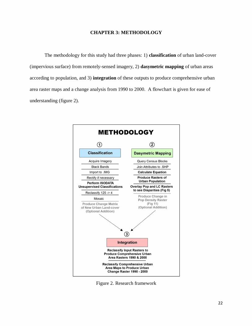
The methodology for this study had three phases: 1) classification of urban land-cover
(impervious surface) from remotely-sensed imagery, 2) dasymetric mapping of urban areas
according to population, and 3) integration of these outputs to produce comprehensive urban
area raster maps and a change analysis from 1990 to 2000. A flowchart is given for ease of
understanding (figure 2).
Figure 2. Research framework

23
3.1 Data Sources and Analysis Extent
Two Landsat TM and two Enhanced Thematic Mapper plus (ETM+) satellite images
were used, dated October 4 and 11, 1989 and October 2 and 9, 2000, respectively. The October
11 and October 9 images covered the western 90% of the study area (Path 24, Row 33), while the
October 4 and October 2 images covered the far eastern portion of the metro area (Path 23, Row
33). These along with the large-scale DOQs for ground truth came from the United States
Geological Survey (USGS). The DOQs were selected randomly, covered the entire range of
possible land-covers, and were reasonably dispersed throughout the analysis extent. They were
identified by the municipal body nearest to or making up most of the image. DOQs from
February 20, 1990 were of Chesterfield and O’Fallon (MO) while DOQs from April 8, 1990
were of Florissant and Webster Groves. DOQs from April 2, 1998 were of Granite City,
Cahokia, Webster Groves, and Alton, while DOQs from March 29, 1999 were of Oakville and
Kampville. Census block and summary tape file (STF) data for the 1990 and 2000 censuses
came from the US Bureau of the Census. The STFs contained population data that were joined
to the geometric TIGER files.
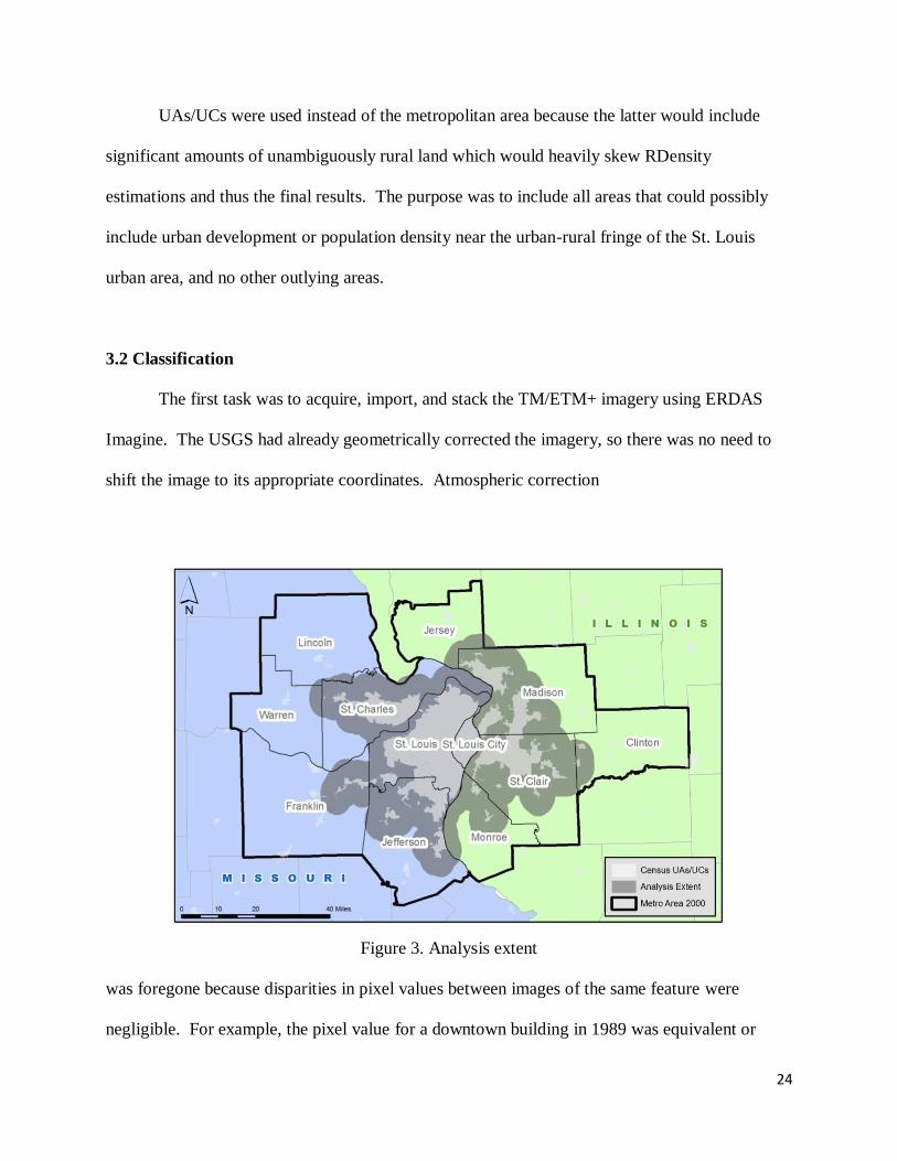
The analysis extent (figure 3) was determined using the Census’ St. Louis Urbanized
Area (UA) in 2000. A UA is a densely settled area containing at least 50,000 people, while an
Urban Cluster (UC) has that between 2,500 and 49,999 population. Both consist of ―core
census block groups or blocks that have a population density of at least 1,000 people per square
mile, and surrounding census blocks that have an overall density of at least 500 people per
square mile‖ (US Census Bureau Geography Division 2009). First, all UAs or UCs within 5
miles of the St. Louis UA were selected. Then this selection was buffered by 5 miles to arrive at
the full analysis extent.
24
UAs/UCs were used instead of the metropolitan area because the latter would include
significant amounts of unambiguously rural land which would heavily skew RDensity
estimations and thus the final results. The purpose was to include all areas that could possibly
include urban development or population density near the urban-rural fringe of the St. Louis
urban area, and no other outlying areas.
3.2 Classification
The first task was to acquire, import, and stack the TM/ETM+ imagery using ERDAS
Imagine. The USGS had already geometrically corrected the imagery, so there was no need to
shift the image to its appropriate coordinates. Atmospheric correction
Figure 3. Analysis extent
was foregone because disparities in pixel values between images of the same feature were
negligible. For example, the pixel value for a downtown building in 1989 was equivalent or
25
nearly equivalent (+/- 3 pixel values) to the corresponding pixel value for that building in 2000.
Next, the ISODATA algorithm was used to produce an unsupervised classification with 125
classes. These were then manually classified into the four land-cover categories: impervious
surface, vegetation, soil/bare earth, and water.
Because a single image did not cover the entire study area, the far eastern portions of the
study area in Illinois were mosaicked in after classification. Mosaic after classification produced
a more accurate classification than before because of differences in atmospheric attenuation
between the images. Rather than attempt atmospheric correction between images after mosaic, it
was easier to classify the images from their original values, then mosaic.
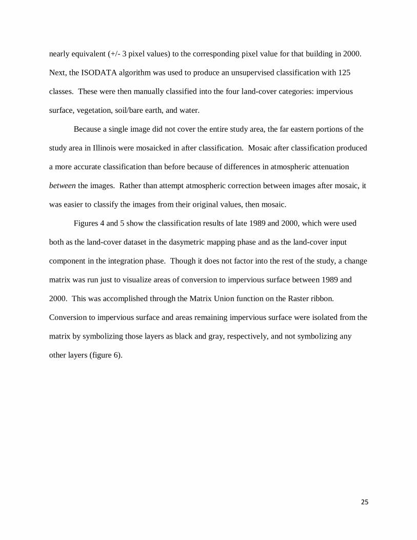
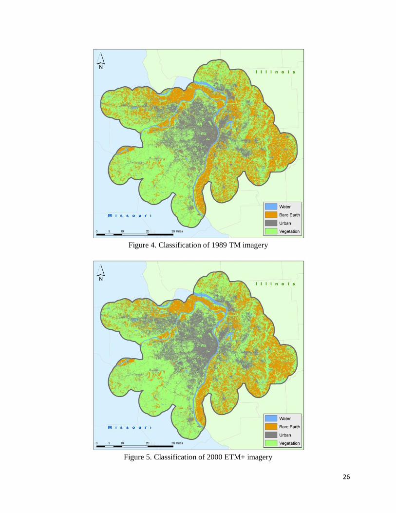
Figures 4 and 5 show the classification results of late 1989 and 2000, which were used
both as the land-cover dataset in the dasymetric mapping phase and as the land-cover input
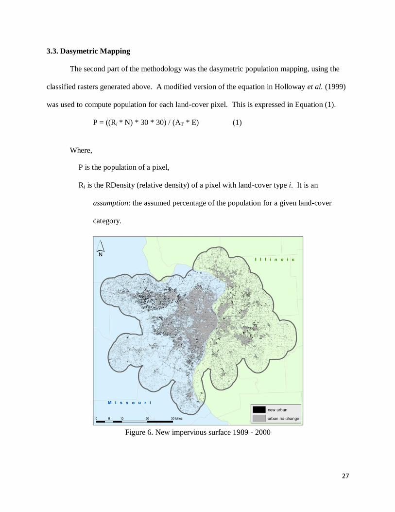
component in the integration phase. Though it does not factor into the rest of the study, a change
matrix was run just to visualize areas of conversion to impervious surface between 1989 and
2000. This was accomplished through the Matrix Union function on the Raster ribbon.
Conversion to impervious surface and areas remaining impervious surface were isolated from the
matrix by symbolizing those layers as black and gray, respectively, and not symbolizing any
other layers (figure 6).
26
Figure 4. Classification of 1989 TM imagery
Figure 5. Classification of 2000 ETM+ imagery
27
3.3. Dasymetric Mapping
The second part of the methodology was the dasymetric population mapping, using the
classified rasters generated above. A modified version of the equation in Holloway et al. (1999)
was used to compute population for each land-cover pixel. This is expressed in Equation (1).
P = ((Ri * N) * 30 * 30) / (AT * E) (1)
Where,
P is the population of a pixel,
Ri is the RDensity (relative density) of a pixel with land-cover type i. It is an
assumption: the assumed percentage of the population for a given land-cover
category.
Figure 6. New impervious surface 1989 - 2000
28
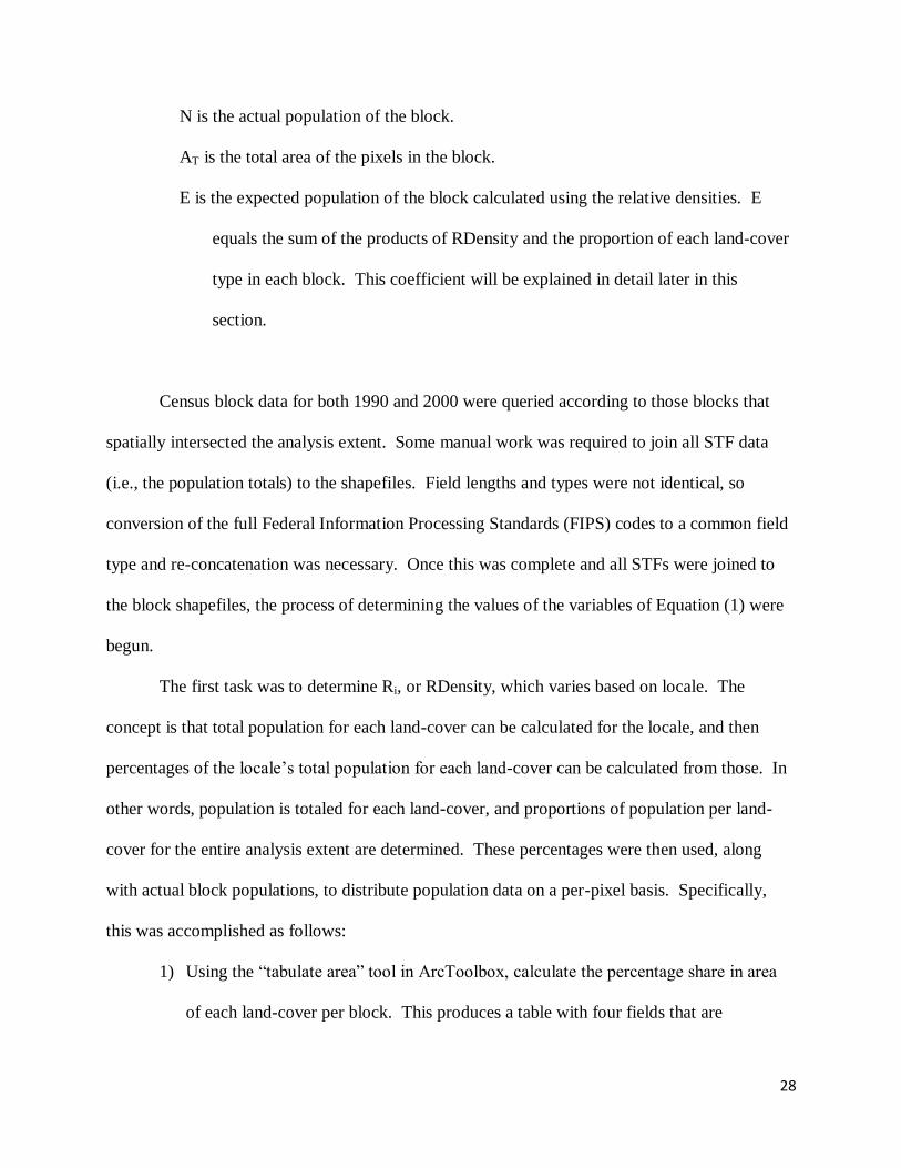
N is the actual population of the block.
AT is the total area of the pixels in the block.
E is the expected population of the block calculated using the relative densities. E
equals the sum of the products of RDensity and the proportion of each land-cover
type in each block. This coefficient will be explained in detail later in this
section.
Census block data for both 1990 and 2000 were queried according to those blocks that
spatially intersected the analysis extent. Some manual work was required to join all STF data
(i.e., the population totals) to the shapefiles. Field lengths and types were not identical, so
conversion of the full Federal Information Processing Standards (FIPS) codes to a common field
type and re-concatenation was necessary. Once this was complete and all STFs were joined to
the block shapefiles, the process of determining the values of the variables of Equation (1) were
begun.
The first task was to determine Ri, or RDensity, which varies based on locale. The
concept is that total population for each land-cover can be calculated for the locale, and then
percentages of the locale’s total population for each land-cover can be calculated from those. In
other words, population is totaled for each land-cover, and proportions of population per land-
cover for the entire analysis extent are determined. These percentages were then used, along
with actual block populations, to distribute population data on a per-pixel basis. Specifically,
this was accomplished as follows:
1) Using the ―tabulate area‖ tool in ArcToolbox, calculate the percentage share in area
of each land-cover per block. This produces a table with four fields that are

29
automatically named according to the field used to tabulate the area, in this case the
―value‖ field, and the numeric value assigned to each land-cover. These fields are
VALUE_1 (urban land-cover), VALUE_2 (vegetation), VALUE_3 (soil), and
VALUE_4 (water). The values for these fields are the square area in meters of each
land-cover in the block.
2) Join the output table to the blocks shapefile.
3) Create a new field called AREA_SUM and calculate it as the sum of the land-cover
area in the block (VALUE_1 + VALUE_2 + VALUE_3 + VALUE_4).
4) Create four new fields, name them USHARE (for ―urban share‖), VSHARE,
SSHARE, and WSHARE, and derive the percentages of each land-cover in the block
by dividing VALUE_1 by AREA_SUM for USHARE, VALUE_2 by AREA_SUM
for VSHARE, and so forth.
5) Create four new fields, name them UPOP, VPOP, SPOP, and WPOP, and calculate
them by multiplying the percentages of each land-cover in the block by the
population of the block—for example, for UPOP, multiply USHARE times POP2000.
6) Sum the population of each land-cover.
7) Divide each sum by the total population for all land-covers to determine the
percentage share of population for each land-cover in the analysis extent.
8) The results can be checked by comparing the total population for all land-covers with
the total population in the original blocks dataset. If they are equivalent, the results
are accurate.
30
This produced the following RDensity assumptions for 1990: 68% urban, 27% vegetation, 5%
soil, and 0% water/wetland (table 1). For 2000, it produced: 70% urban, 27% vegetation, 2%
soil, and 1% water/wetland. The 1% of population in water/wetland areas was due to water
forming some of the land-cover of blocks with population.
It should be emphasized that RDensity is an average derived from the entire analysis
extent. For instance, for the 2000 urban RDensity value of 70%, a largely abandoned
neighborhood in north St. Louis city and a high density city block in the Central West End
neighborhood contribute unequally to the 70% fraction. Both areas are of urban land-cover but
do not contribute equally to the sum of population for the urban land-cover across the study area.
Nonetheless, the 70% factor is then applied back on both areas, indiscriminately, in the equation.
One might think that this translates into under- or overestimating blocks that are statistical
outliers for their land-cover. However, this effect is minimized by the values which the
RDensity factors are multiplied by—the populations of the block. Furthermore, on the scale of
the entire study area, this method provides the most balanced results.

31
Table 1. RDensity values
urban vegetation soil water TOTAL
1990 1,542,957 608,703 106,838 2,967 2,261,465
percentage 68% 27% 5% 0%
2000 1,640,646 638,804 52,443 9,549 2,341,442
percentage 70% 27% 2% 1%
LAND-COVER
P
OPU
LATI
ON
The next step was to determine the other variables of Equation (1). Rasters were
produced of both RDensity and block population. The RDensity raster was a raster of land-cover
with the RDensity percentages (e.g., 68, 27, 2…) as the values of each land-cover category. The
block population raster was a raster of the census blocks with the population as the value for
each pixel of the block. To calculate E, the expectation of what population a block should have
based on RDensity and its land-cover share, a raster of FIPS codes was produced. (FIPS codes
are unique block IDs.) Then the area of each land-cover was tabulated per block (i.e., per FIPS
code) in square meters by using the FIPS raster as the zonal dataset. Percentages were derived
from the area numbers by adding five fields: total, urban, vegetation, soil, and water. The
―Total‖ field was calculated for the total square meters tabulated for the block, and the other
urban, vegetation, soil, and water fields were calculated as the quotient of the tabulated area of
the given land-cover over the ―Total‖ field. An ―Expect‖ field was then calculated by
multiplying the land-cover share of a block by RDensity. Equation (2) shows how the ―Expect‖
field was calculated for 2000.
Expect = urban * 70 + vegetation * 27 + soil * 2 + water * 1 (2)
32
For example, this would produce an expect value of 27 persons for a block that had a
land-cover share of 100% vegetation (1 * 27 = 27). For a block that is 1/5th urban and 4/5ths
vegetation it produces an expect value of 53.6 (0.2 * 70 + 0.8 * 27 = 14 + 21.6 = 35.6). For a
block that is 3/8ths urban, 4/8ths vegetation, and 1/8th soil, it produces 40 (0.375 * 70 + 0.5 * 27
+ 0.125 * 2 = 26.25 + 13.5 + 0.25 = 40).
To create rasters of the final two variables, the area of each block and the expected
population of each block, the tabulate area table with the ―Expect‖ field was joined to the main
shapefile containing all blocks. A raster was created of the total area in a block (blockarea).
This variable is for data standardization by area, to determine the population count per square
meters in the block. A raster was also created of the expected population of a block
(blockexpect). These were the final two variables to determine before calculation of Equation
(1). The final calculation can be expressed in Expression (1):
Rdensity * blockpopulation * 30 * 30 / (blockarea * blockexpect) (1)
The logic of this expression is as follows. As an example, assume the following values
for Expression (1):
68 * 422 * 30 * 30 / (46,800 * 68)
If one ignores the 30 * 30 temporarily, this equation is easier to digest. RDensity is a factor, for
example, urban, so its value is 68. That is multiplied by the population of the block, 422.
Looking at the denominator, the area of the block is 46,800 square meters. That is multiplied by
the expect value, also 68. The 32s cancel out. What is left is the block population over the block

33
area: 422 / 46,800. This is a measure of persons per square meters. But it is not at the pixel
level, which is the geometric unit corresponding to our tabular data here, the data for the pixel.
In this state, it is at the block level. The entire expression must be divided by the area of the
pixel: 30 * 30. This is accomplished by multiplying the numerator by the square meters of the
pixel, 900. The equation itself makes little sense when its relationship to the pixel is not
considered, but insofar as it is applied in the map, it is apparent that the numerator must be
multiplied by the factor of a pixel’s area. Thus 422 is multiplied by 900 which equals 379,800.
That is divided by 46,800 which equals 8.12 persons for that pixel.
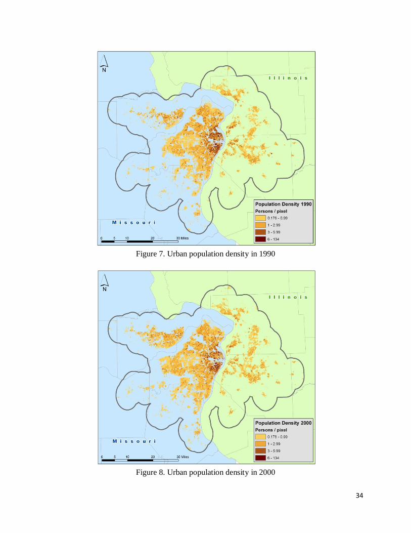
Figures 7 and 8 show the dasymetric results for both 1990 and 2000. To indicate only
urban areas, all cells calculated to be below 500 persons per square mile—the Census definition
for outlying areas of an Urban Cluster, which is ―the lesser urban‖ of the two urban categories—
were reclassified to zero. The conversion of 500 people/square mile to the pixel level using 30 x
30-meter imagery is 0.176 persons/pixel.
As to verifying volume-preservation (the so-called pycnophylactic property) of the
disaggregated population totals from blocks to pixel, calculation of zonal statistics for blocks on
the output population rasters through Spatial Analyst produced equivalent population values to
original block population values. That is, a population value for any given block in the original
census data was equivalent to the sum of population values for all pixels in that original block.
This verified that all population values going into the disaggregation appeared in the results (i.e.,
that no population was effectively created or disappeared).
34
Figure 7. Urban population density in 1990
Figure 8. Urban population density in 2000
35
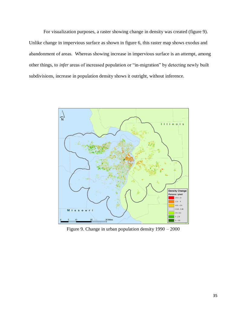
For visualization purposes, a raster showing change in density was created (figure 9).
Unlike change in impervious surface as shown in figure 6, this raster map shows exodus and
abandonment of areas. Whereas showing increase in impervious surface is an attempt, among
other things, to infer areas of increased population or ―in-migration‖ by detecting newly built
subdivisions, increase in population density shows it outright, without inference.
Figure 9. Change in urban population density 1990 – 2000
36
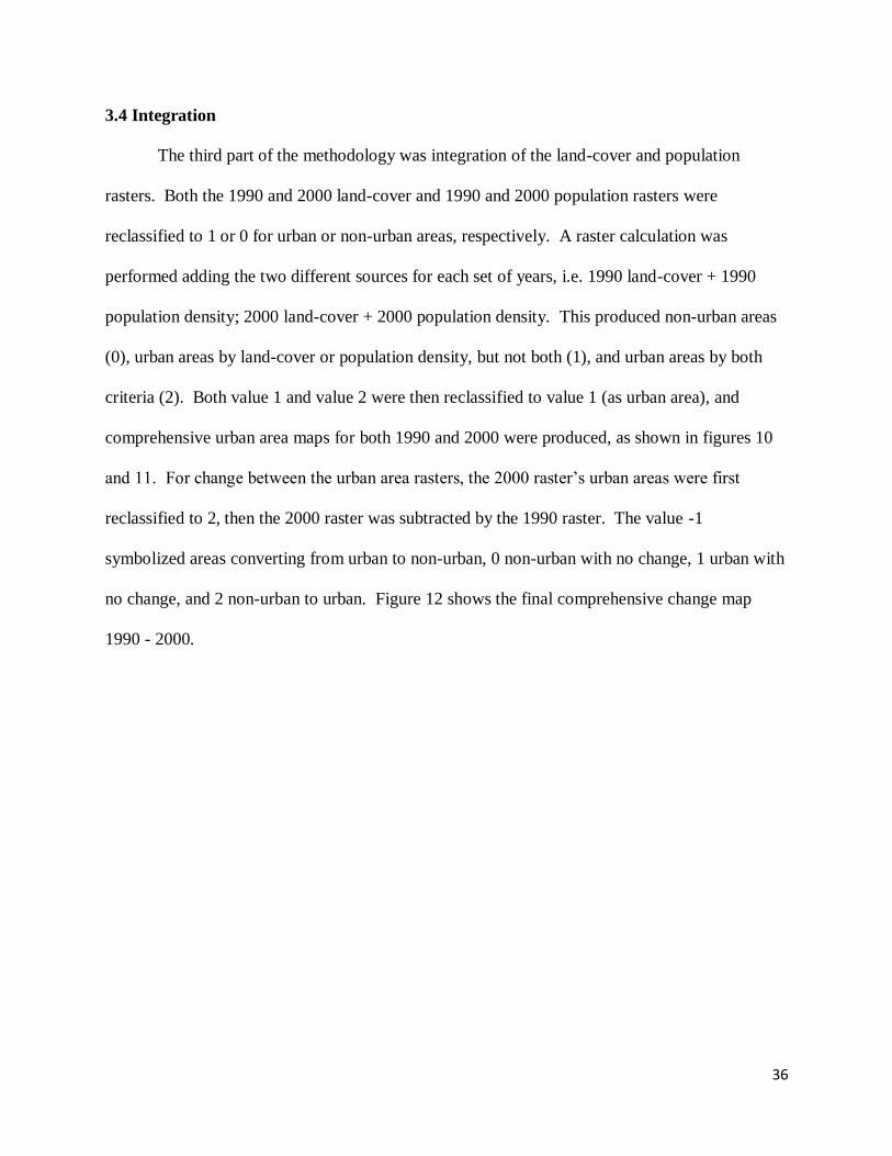
3.4 Integration
The third part of the methodology was integration of the land-cover and population
rasters. Both the 1990 and 2000 land-cover and 1990 and 2000 population rasters were
reclassified to 1 or 0 for urban or non-urban areas, respectively. A raster calculation was
performed adding the two different sources for each set of years, i.e. 1990 land-cover + 1990
population density; 2000 land-cover + 2000 population density. This produced non-urban areas
(0), urban areas by land-cover or population density, but not both (1), and urban areas by both
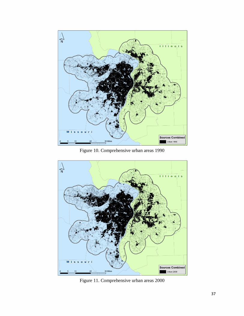
criteria (2). Both value 1 and value 2 were then reclassified to value 1 (as urban area), and
comprehensive urban area maps for both 1990 and 2000 were produced, as shown in figures 10
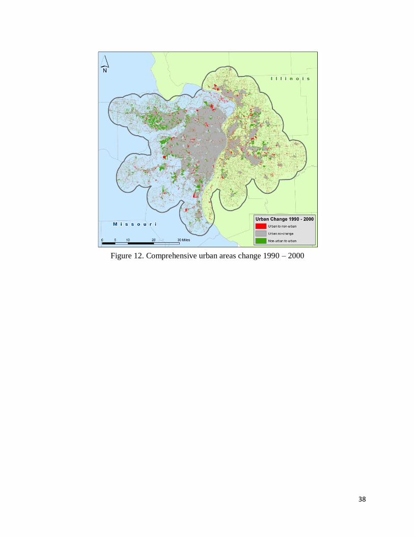
and 11. For change between the urban area rasters, the 2000 raster’s urban areas were first
reclassified to 2, then the 2000 raster was subtracted by the 1990 raster. The value -1
symbolized areas converting from urban to non-urban, 0 non-urban with no change, 1 urban with
no change, and 2 non-urban to urban. Figure 12 shows the final comprehensive change map
1990 - 2000.
37
Figure 10. Comprehensive urban areas 1990
Figure 11. Comprehensive urban areas 2000
38
Figure 12. Comprehensive urban areas change 1990 – 2000
39
CHAPTER 4: ANALYSIS RESULTS
4.1 Where was the Change and Why?
Most of the differences between urban areas in 1990 and 2000 are on the urban/rural
fringe. Indeed, since the 1980s, development on the rural fringes has expanded to cover more
square miles than central cities, older suburbs, and edge nodes combined (Hayden 2003).
To determine why these areas experienced conversion—by land-cover or urban
population density—the urban change raster was reclassified into two different datasets: one
consisting just of non-urban to urban conversion, the other of urban to non-urban conversion.
These were both then converted to vector and intersected with the following datasets based on
which of the two types of land-cover conversion they showed:
a) if urban to non-urban conversion, intersected separately with each of the 1990 urban
by population and urban by land-cover rasters.
b) if non-urban to urban, intersected separately with each of the 2000 urban by
population and urban by land-cover rasters.
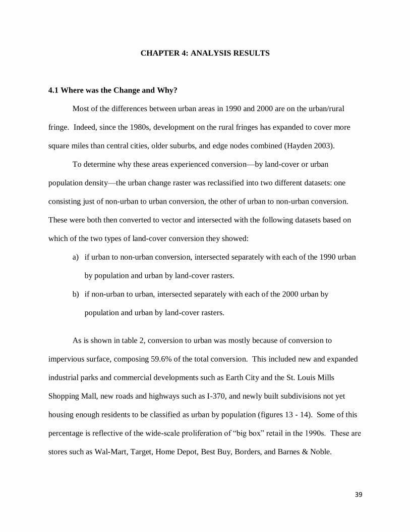
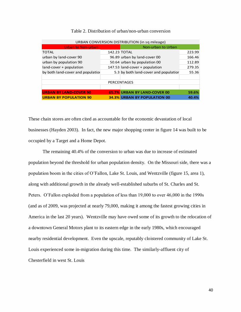
As is shown in table 2, conversion to urban was mostly because of conversion to
impervious surface, composing 59.6% of the total conversion. This included new and expanded
industrial parks and commercial developments such as Earth City and the St. Louis Mills
Shopping Mall, new roads and highways such as I-370, and newly built subdivisions not yet
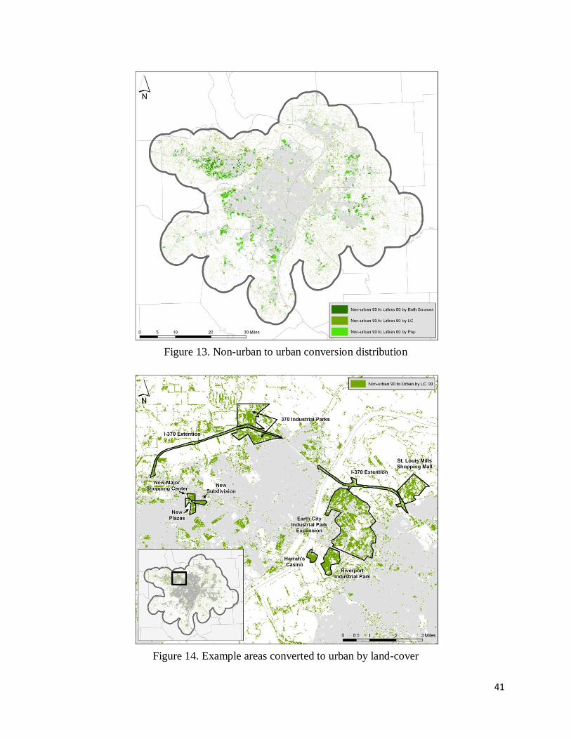
housing enough residents to be classified as urban by population (figures 13 - 14). Some of this
percentage is reflective of the wide-scale proliferation of ―big box‖ retail in the 1990s. These are
stores such as Wal-Mart, Target, Home Depot, Best Buy, Borders, and Barnes & Noble.
40
Table 2. Distribution of urban/non-urban conversion
TOTAL 142.23 TOTAL 223.99
urban by land-cover 90 96.89 urban by land-cover 00 166.46
urban by population 90 50.64 urban by population 00 112.89
land-cover + population 147.53 land-cover + population 279.35
by both land-cover and population 5.3 by both land-cover and population 55.36
URBAN BY LAND-COVER 90 65.7% URBAN BY LAND-COVER 00 59.6%
URBAN BY POPULATION 90 34.3% URBAN BY POPULATION 00 40.4%
URBAN CONVERSION DISTRIBUTION (in sq mileage)
Urban to Non-urban Non-urban to Urban
PERCENTAGES
These chain stores are often cited as accountable for the economic devastation of local
businesses (Hayden 2003). In fact, the new major shopping center in figure 14 was built to be
occupied by a Target and a Home Depot.
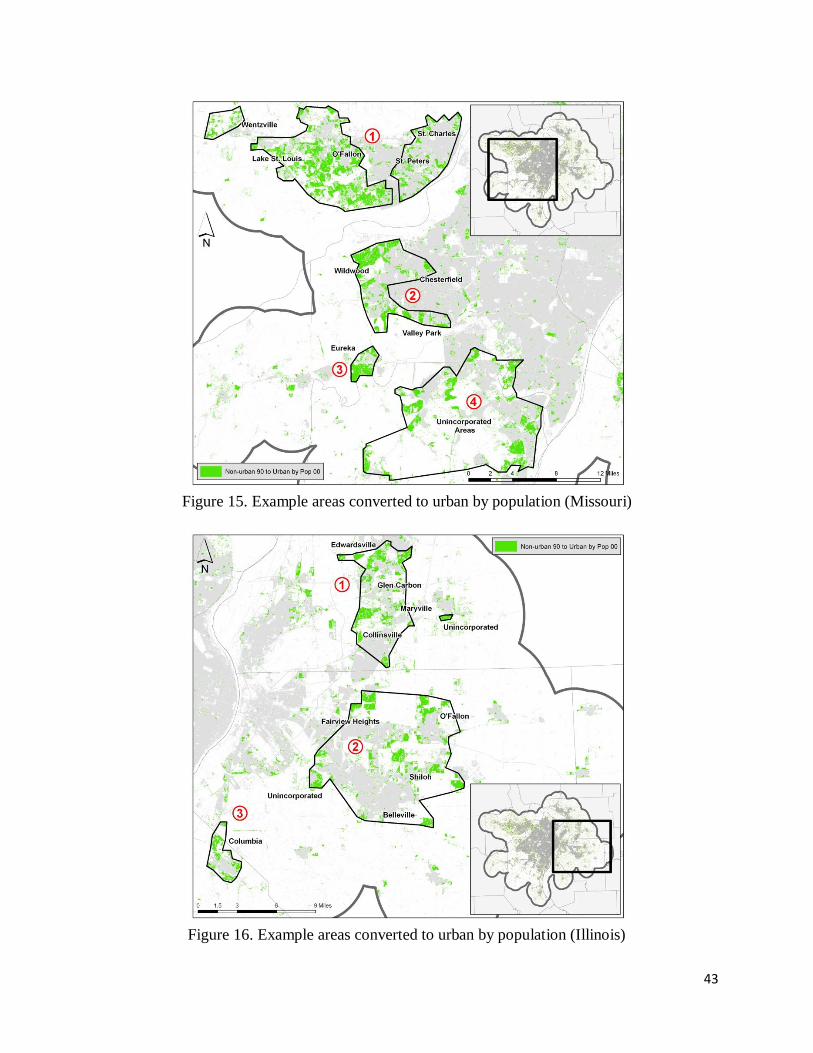
The remaining 40.4% of the conversion to urban was due to increase of estimated
population beyond the threshold for urban population density. On the Missouri side, there was a
population boom in the cities of O’Fallon, Lake St. Louis, and Wentzville (figure 15, area 1),
along with additional growth in the already well-established suburbs of St. Charles and St.
Peters. O’Fallon exploded from a population of less than 19,000 to over 46,000 in the 1990s
(and as of 2009, was projected at nearly 79,000, making it among the fastest growing cities in
America in the last 20 years). Wentzville may have owed some of its growth to the relocation of
a downtown General Motors plant to its eastern edge in the early 1980s, which encouraged
nearby residential development. Even the upscale, reputably cloistered community of Lake St.
Louis experienced some in-migration during this time. The similarly-affluent city of
Chesterfield in west St. Louis
41
Figure 13. Non-urban to urban conversion distribution
Figure 14. Example areas converted to urban by land-cover
42
county also experienced growth, but it was Wildwood, incorporated in 1995, that erupted onto
the map with 32,884 residents in 2000 (area 2). This sprawling municipality was driven to
incorporation ―largely by fears that St. Louis County was not willing to sustain
large-lot single-family residential development‖ (Gordon 2008 p.41). Population in the exurb of
Eureka along I-44 also met the threshold density for urban (area 3), as well as unincorporated
areas in Jefferson County and St. Louis County (area 4).
On the Illinois side, growth in population also seemed to be primarily dictated by
proximity to major highways. The continuous urban swath of Edwardsville, Glen Carbon,
Maryville, and Collinsville (figure 16, area 1) near I-270 experienced significant growth, as did
Fairview Heights, O’Fallon, and Shiloh near I-64 (area 2). The City of Columbia, south off of I-
255, showed several pockets of population exceeding the urban threshold (area 3).
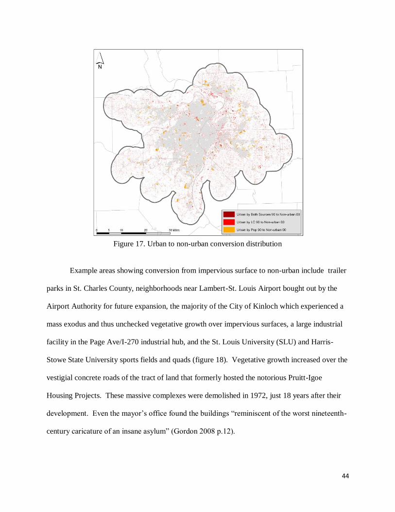
Conversion to non-urban was dominated by land-cover change as well (figure 17). An
estimated 20-25% of this is made up by urban misclassifications in the 1990 classification. This
is because of the similar reflectivity of some farmland to certain impervious surfaces. In fact the
main difficulty encountered with classification was how different surfaces reflect light similarly
and thus cause a confused classification. Shadows of downtown skyscrapers, for instance, were
often mistaken for water and required manual correction (by converting the pixel value to an
impervious surface value averaged for the pixel neighborhood). Significant areas of floodplain
were confused as areas of impervious surface as well.
43
Figure 15. Example areas converted to urban by population (Missouri)
Figure 16. Example areas converted to urban by population (Illinois)
44
Figure 17. Urban to non-urban conversion distribution
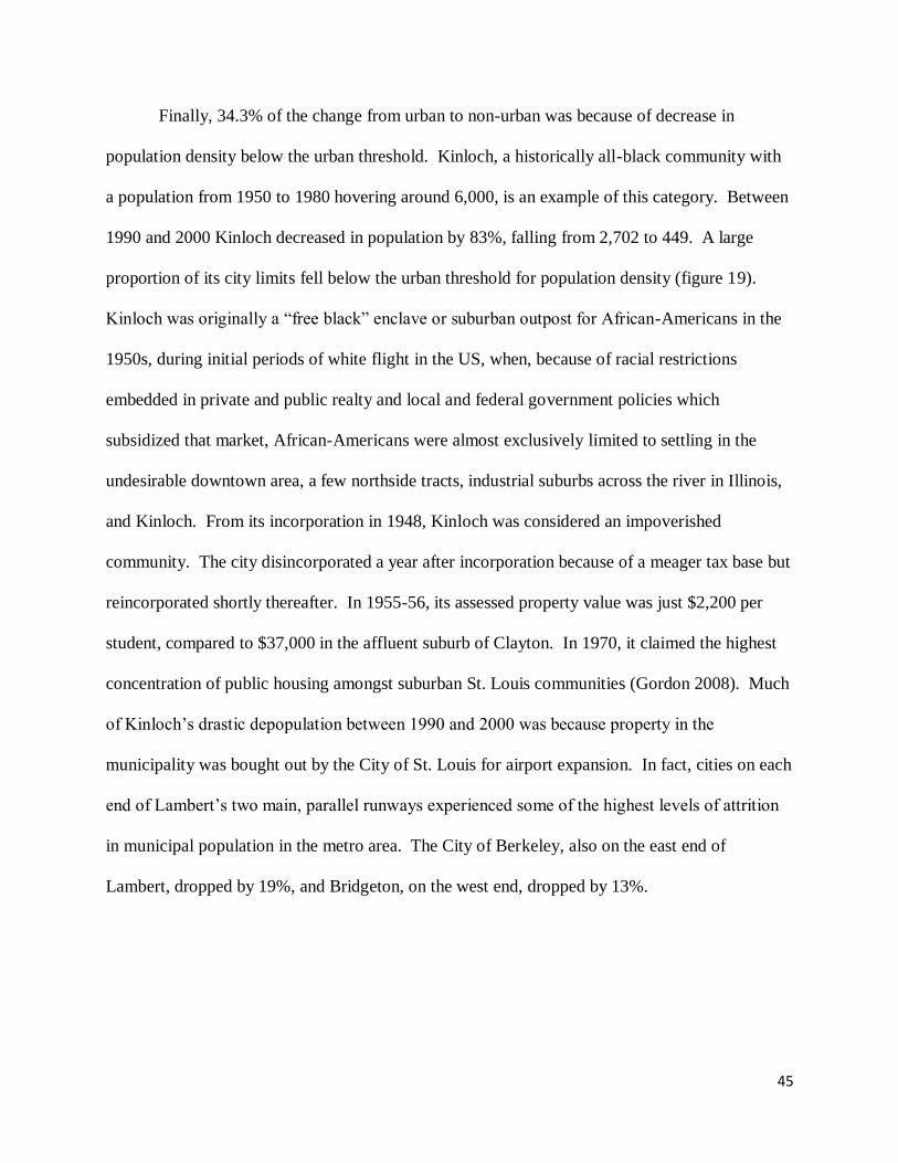
Example areas showing conversion from impervious surface to non-urban include trailer
parks in St. Charles County, neighborhoods near Lambert-St. Louis Airport bought out by the
Airport Authority for future expansion, the majority of the City of Kinloch which experienced a
mass exodus and thus unchecked vegetative growth over impervious surfaces, a large industrial
facility in the Page Ave/I-270 industrial hub, and the St. Louis University (SLU) and Harris-
Stowe State University sports fields and quads (figure 18). Vegetative growth increased over the
vestigial concrete roads of the tract of land that formerly hosted the notorious Pruitt-Igoe
Housing Projects. These massive complexes were demolished in 1972, just 18 years after their
development. Even the mayor’s office found the buildings ―reminiscent of the worst nineteenth-
century caricature of an insane asylum‖ (Gordon 2008 p.12).
45
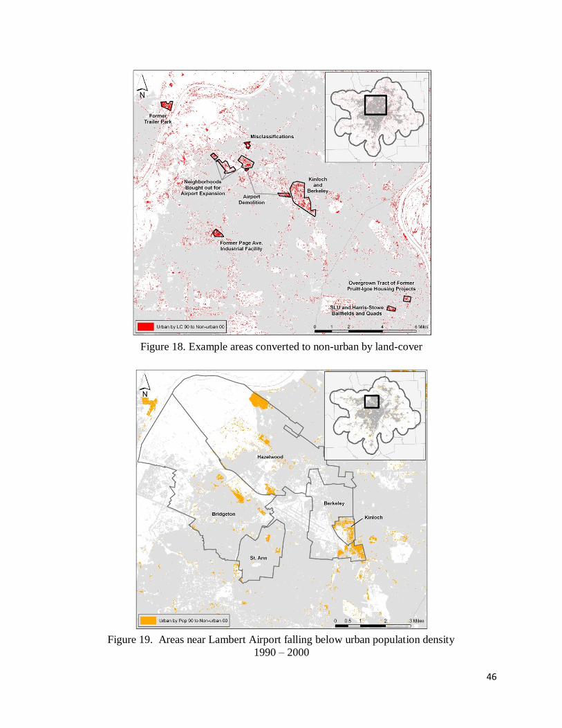
Finally, 34.3% of the change from urban to non-urban was because of decrease in
population density below the urban threshold. Kinloch, a historically all-black community with
a population from 1950 to 1980 hovering around 6,000, is an example of this category. Between
1990 and 2000 Kinloch decreased in population by 83%, falling from 2,702 to 449. A large
proportion of its city limits fell below the urban threshold for population density (figure 19).
Kinloch was originally a ―free black‖ enclave or suburban outpost for African-Americans in the
1950s, during initial periods of white flight in the US, when, because of racial restrictions
embedded in private and public realty and local and federal government policies which
subsidized that market, African-Americans were almost exclusively limited to settling in the
undesirable downtown area, a few northside tracts, industrial suburbs across the river in Illinois,
and Kinloch. From its incorporation in 1948, Kinloch was considered an impoverished
community. The city disincorporated a year after incorporation because of a meager tax base but
reincorporated shortly thereafter. In 1955-56, its assessed property value was just $2,200 per
student, compared to $37,000 in the affluent suburb of Clayton. In 1970, it claimed the highest
concentration of public housing amongst suburban St. Louis communities (Gordon 2008). Much
of Kinloch’s drastic depopulation between 1990 and 2000 was because property in the
municipality was bought out by the City of St. Louis for airport expansion. In fact, cities on each
end of Lambert’s two main, parallel runways experienced some of the highest levels of attrition
in municipal population in the metro area. The City of Berkeley, also on the east end of
Lambert, dropped by 19%, and Bridgeton, on the west end, dropped by 13%.
46
Figure 18. Example areas converted to non-urban by land-cover
Figure 19. Areas near Lambert Airport falling below urban population density
1990 – 2000
47
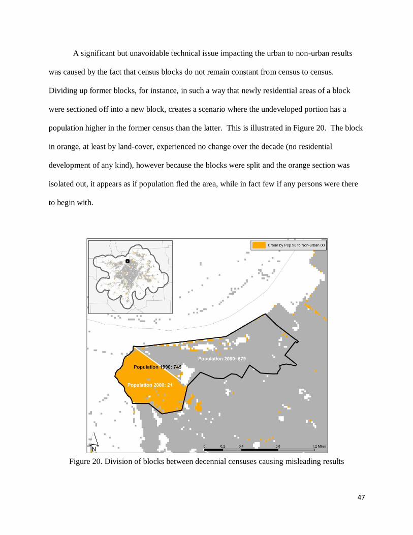
A significant but unavoidable technical issue impacting the urban to non-urban results
was caused by the fact that census blocks do not remain constant from census to census.
Dividing up former blocks, for instance, in such a way that newly residential areas of a block
were sectioned off into a new block, creates a scenario where the undeveloped portion has a
population higher in the former census than the latter. This is illustrated in Figure 20. The block
in orange, at least by land-cover, experienced no change over the decade (no residential
development of any kind), however because the blocks were split and the orange section was
isolated out, it appears as if population fled the area, while in fact few if any persons were there
to begin with.
Figure 20. Division of blocks between decennial censuses causing misleading results
48
4.2 Density Change in and near the City
Referring back to the density change raster map (figure 9), there were areas that
decreased in population at various increments, without falling below the urban threshold. Like
the decades before, a significant drop in population afflicted St. Louis city in the 1990s: from
396,685 to 348,189. In fact, since its peak just over 850,000 in 1950, the city dropped an
average 10,000 persons per year in the latter half of the 20th
century, at an accelerating rate up
until 1980: population 750,000 in 1960, 622,000 in 1970, 453,000 in 1980, 397,000 in 1990, and
348,000 in 2000. The northern half in particular has experienced mass exodus and neglect. In
1956, a visiting French businessman noted that the view from Monsanto’s downtown
headquarters ―look[ed] like a European city bombed in the war‖ (Gordon 2008 p.11). By 1978,
St. Louis had the highest vacancy rate (just under 10 percent) of all central cities. When the city
challenged the results of the 1980 census, officials responded by rubbing it in:
“If they don’t wake up and acknowledge the exodus, they’re going to lose it all. They
ought to get out of their offices and drive through north St. Louis. A lot of it looks like a
ghost town. When we come back to count in 1990, it may not even be a city. It may be a
village.” (Gordon 2008 p.23)
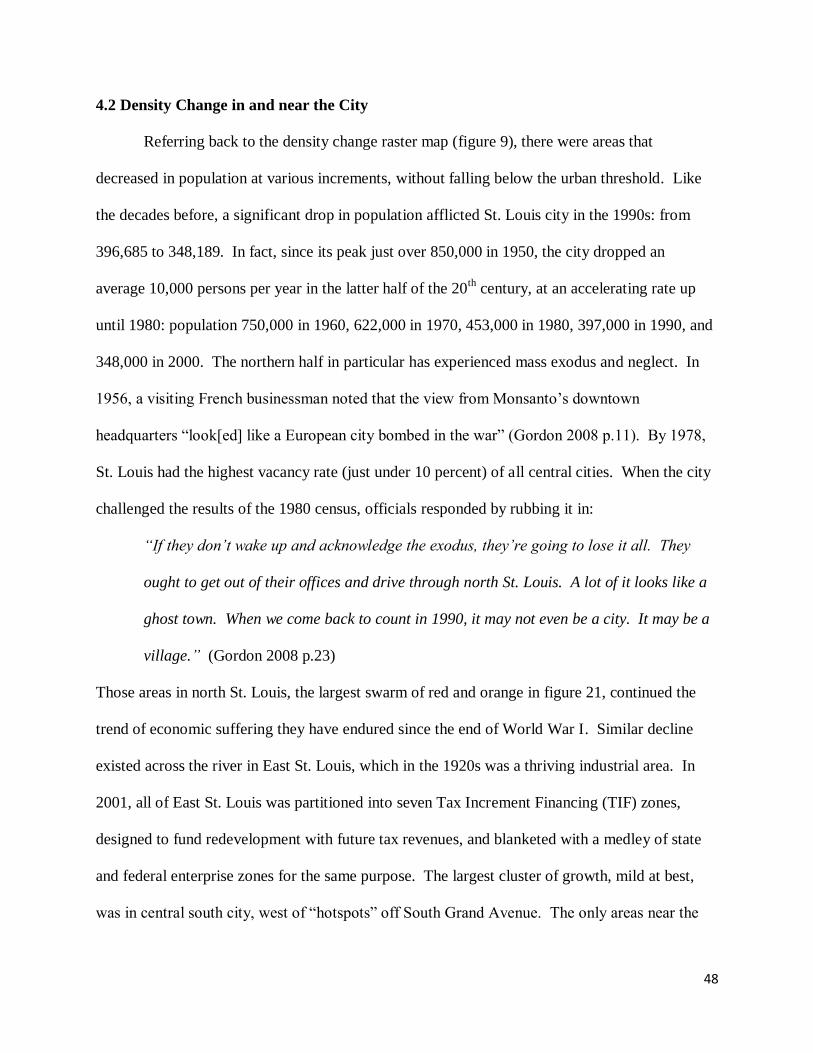
Those areas in north St. Louis, the largest swarm of red and orange in figure 21, continued the
trend of economic suffering they have endured since the end of World War I. Similar decline
existed across the river in East St. Louis, which in the 1920s was a thriving industrial area. In
2001, all of East St. Louis was partitioned into seven Tax Increment Financing (TIF) zones,
designed to fund redevelopment with future tax revenues, and blanketed with a medley of state
and federal enterprise zones for the same purpose. The largest cluster of growth, mild at best,
was in central south city, west of ―hotspots‖ off South Grand Avenue. The only areas near the
49
city of appreciable population growth is Washington University’s (WashU) Danforth (main)
campus property, due to the building of new housing (mostly for students), and residential areas
in University City near the popular Delmar Boulevard strip. The latter’s growth is probably due
to both increased university enrollment and proximity to the major office center of Clayton, the
de facto central business district of the metro (Gordon 2008 p.20). Interestingly, Washington
University in St. Louis’ main campus is an unincorporated island, surrounded by St. Louis to the
east, University City to the north and west, and Clayton to the south.
Figure 21. Population density change in and near St. Louis city 1990 – 2000
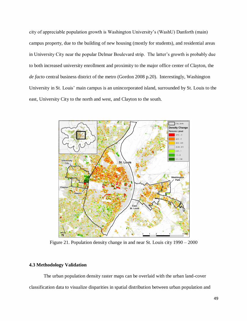
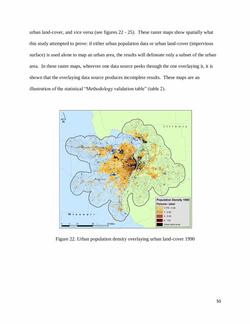
4.3 Methodology Validation
The urban population density raster maps can be overlaid with the urban land-cover
classification data to visualize disparities in spatial distribution between urban population and
50
urban land-cover, and vice versa (see figures 22 - 25). These raster maps show spatially what
this study attempted to prove: if either urban population data or urban land-cover (impervious
surface) is used alone to map an urban area, the results will delineate only a subset of the urban
area. In these raster maps, wherever one data source peeks through the one overlaying it, it is
shown that the overlaying data source produces incomplete results. These maps are an
illustration of the statistical ―Methodology validation table‖ (table 2).
Figure 22. Urban population density overlaying urban land-cover 1990
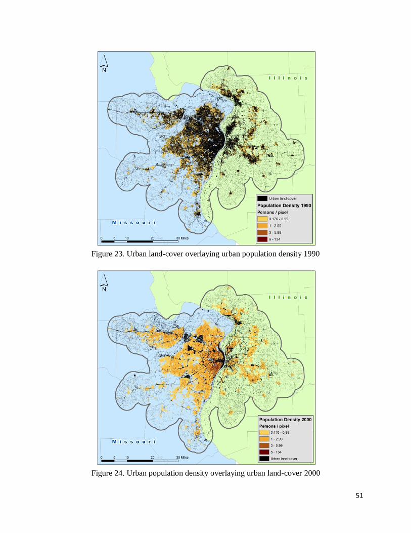
51
Figure 23. Urban land-cover overlaying urban population density 1990
Figure 24. Urban population density overlaying urban land-cover 2000
52
To determine how much urban area is excluded using only remotely-sensed data or only
population data, the square mileage of each were totaled and divided over the square mileage of
the combined urban area to arrive at percentages showing the comprehensiveness of each data
source by itself. This is shown in table 3. For both years, using only one data source detects
only 71 to 73% of the urban area, relative to use of both sources. This stresses the necessity of
using population totals and LULC classifications together.
Figure 25. Urban land-cover overlaying urban population density 2000
53
Table 3. Methodology validation table – percentages of urban area covered by only one data
source
DATASET 1990 sq mileage 2000 sq mileage
urban land-cover 554.31 629.33
urban population 568.67 625.17
urban combined 776.56 858.54
urban land-cover ONLY 71.4% 73.3%
urban population ONLY 73.2% 72.8%
PERCENTAGES
4.4 Accuracy Assessment
The accuracy of the final output of this study can only be measured to an extent, due to
the limitations inherent in checking the output of dasymetric mapping. This is because
dasymetric mapping relies on assumptions such as RDensity rather than verified data to produce
results. Classification accuracies were determined using an error matrix, while dasymetric
accuracies were measured against how the dasymetric results spatially coincided with the
original census block population data.
TM and ETM+ imagery classification accuracies were assessed using an error matrix, as
shown in tables 4 and 5 for 1990 and 2000, respectively. DOQs from the USGS were used as
ground truth data. Due to the large analysis extent, only four DOQs were used for the 1990
classification accuracy assessment (figure 26), and six DOQs were used for the 2000 assessment
(figure 27). Each DOQ measured roughly 7,700 meters from its northern to its southern
extremity. A random number generator was used to select east-west lines of pixels in the
classified raster that intersected with the
54
Table 4. Classification matrix for 1989 TM imagery
urban vegetation soil water TOTAL
urban 349 26 12 0 387 90.2%
vegetation 39 230 9 0 278 82.7%
soil 6 6 244 0 256 95.3%
water 2 2 0 53 57 93.0%
TOTAL 396 264 265 53 978
Producer's Accuracy 88.1% 87.1% 92.1% 100.0% 89.6%
kappa 84.9%
User's Accuracy
Table 5. Classification matrix for 2000 ETM+ imagery
urban vegetation soil water TOTAL
urban 452 28 0 0 480 94.2%
vegetation 55 353 3 0 411 85.9%
soil 8 4 157 0 169 92.9%
water 16 2 9 111 138 80.4%
TOTAL 531 387 169 111 1198
Producer's Accuracy 85.1% 91.2% 92.9% 100.0% 89.6%
kappa 84.7%
User's Accuracy
DOQs. A random number of one represented the northernmost edge of the DOQ while 7,700
represented the southernmost. If, for instance, 2,510 was the random number generated, the
measure tool was used to determine the line of pixels in the classified image corresponding to
2,510 meters from the northern extremity of the DOQ. That line of pixels was then evaluated for
classification accuracy against the same area on the DOQ. For each DOQ, one line of pixels in
the classified image was evaluated. Overall accuracies for the two classifications were identical
at 89.6%, while the kappa coefficient for the 1989 image was 84.9% and that for 2000 was
84.7%.
The accuracies for the dasymetric population mapping were measured against the census
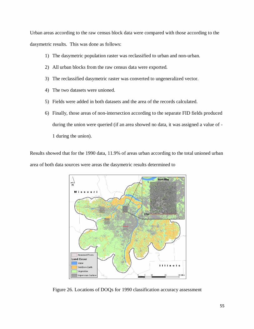
block data used to achieve the dasymetric results—how the results coincided with it or did not.
55
Urban areas according to the raw census block data were compared with those according to the
dasymetric results. This was done as follows:
1) The dasymetric population raster was reclassified to urban and non-urban.
2) All urban blocks from the raw census data were exported.
3) The reclassified dasymetric raster was converted to ungeneralized vector.
4) The two datasets were unioned.
5) Fields were added in both datasets and the area of the records calculated.
6) Finally, those areas of non-intersection according to the separate FID fields produced
during the union were queried (if an area showed no data, it was assigned a value of -
1 during the union).
Results showed that for the 1990 data, 11.9% of areas urban according to the total unioned urban
area of both data sources were areas the dasymetric results determined to
Figure 26. Locations of DOQs for 1990 classification accuracy assessment
56
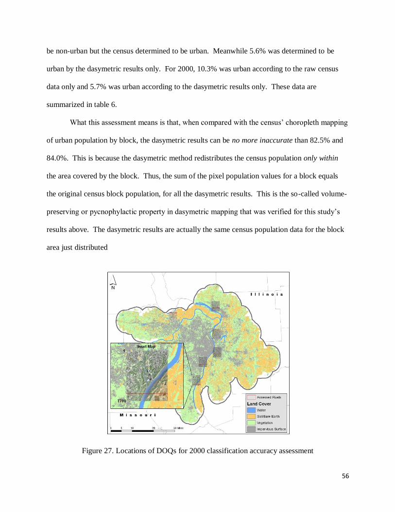
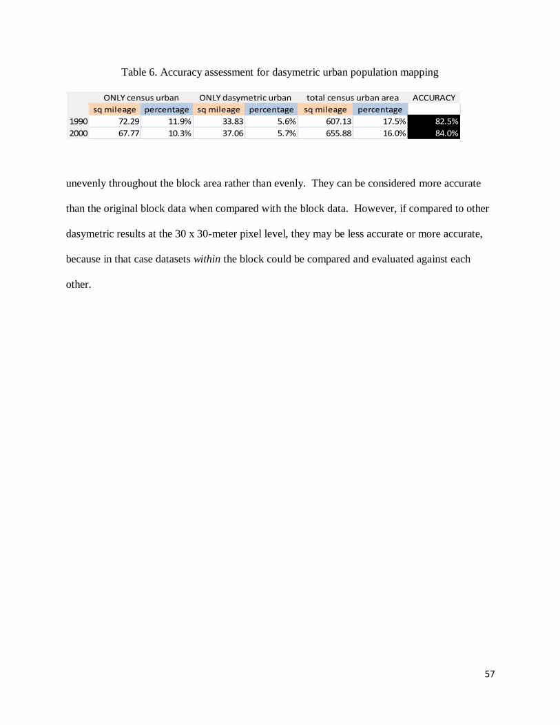
be non-urban but the census determined to be urban. Meanwhile 5.6% was determined to be
urban by the dasymetric results only. For 2000, 10.3% was urban according to the raw census
data only and 5.7% was urban according to the dasymetric results only. These data are
summarized in table 6.
What this assessment means is that, when compared with the census’ choropleth mapping
of urban population by block, the dasymetric results can be no more inaccurate than 82.5% and
84.0%. This is because the dasymetric method redistributes the census population only within
the area covered by the block. Thus, the sum of the pixel population values for a block equals
the original census block population, for all the dasymetric results. This is the so-called volume-
preserving or pycnophylactic property in dasymetric mapping that was verified for this study’s
results above. The dasymetric results are actually the same census population data for the block
area just distributed
Figure 27. Locations of DOQs for 2000 classification accuracy assessment
57
Table 6. Accuracy assessment for dasymetric urban population mapping
ACCURACY
sq mileage percentage sq mileage percentage sq mileage percentage
1990 72.29 11.9% 33.83 5.6% 607.13 17.5% 82.5%
2000 67.77 10.3% 37.06 5.7% 655.88 16.0% 84.0%
ONLY census urban ONLY dasymetric urban total census urban area
unevenly throughout the block area rather than evenly. They can be considered more accurate
than the original block data when compared with the block data. However, if compared to other
dasymetric results at the 30 x 30-meter pixel level, they may be less accurate or more accurate,
because in that case datasets within the block could be compared and evaluated against each
other.
58
CHAPTER 5: CONCLUSION
The purpose of this study was to develop a dasymetric technique for mapping urban areas
and their change over time utilizing two fundamental criteria for an urban environment: urban
population density and the presence of impervious surface. It was shown that when these data
sources are used together, results are more comprehensive than when either data source is used
alone. Either of the data sources used alone would yield only roughly 70% of the urban area as
delineated when both sources are combined. What this means is that the corpus of research on
urban area delineation and growth through the use of optical, aerial remote sensing systems
could very well be only 70% accurate. This could be the case in spite of accuracy assessments
yielding strong results, because of the failure to understand the added dimension that data such as
population data bring to such studies. In other words, remote sensing classifications do not
interpret large-lot, vegetated subdivisions found on urban-rural fringes as urban, but as
vegetation more or less identical to rural areas such as open pastures or forestland. Nor do
classifications see as urban wealthier suburbs only a few miles from the central city limits (such
as Ladue, MO) that have very thick canopies blocking out streets and homes. Admittedly,
satellite imagery with higher spatial resolution may yield more comprehensive results than TM
and ETM+ imagery, but they are likely still to be significantly deficient because of the mixed
pixel problem, vegetative canopies, and phenomena related to the presence and movement of
urban population not readily detectable to optical satellites.
59
5.1 Analysis Problems and Limitations
It is important to explain an error that was committed in the calculation of RDensity in
the early trial of this study. In the procedure detailed on pages 28-29, step five had been
mistakenly omitted. The error had resulted in significantly different values for RDensity, which
slightly affected the overall results in the drafts. Omitting step five did not factor population into
the calculations and the resulting RDensity values were only a measure of the proportions of
land-cover in the study area. Multiplying the percentage of land-cover share for each block by
population of a block weighted the RDensity results according to population, and the RDensity
values were then appropriately a percentage of population for a given land-cover category in the
area.
The error had produced the following RDensity assumptions for 1990: 33% urban, 49%
vegetation, 17% soil, and 1% water/wetland. For 2000, it produced: 32% urban, 59% vegetation,
8% soil, and 1% water/wetland. The high vegetation and lower urban percentages seemed
counterintuitive for an area so heavily urbanized. This was an indication that the calculation was
incorrect. The error was corrected in the final trial of the study, when calculations were repeated
to provide greater elaboration on the process of determining RDensity.
Though this technique accomplished its aim for this study, it is surely not without
limitations, and future research could hone it significantly. A major problem encountered in this
project was the urban/non-urban status of developed land that is physically very similar to rural
land. For instance, many would believe golf courses and urban parks such as Forest Park or
Tower Grove Park in St. Louis city to be urban, in spite of their abundance of vegetative growth.
Their purpose after all is urban, and they experience quite a bit of ―people traffic‖ on a regular
basis (though according to this conception, golf courses might be considered rural during

60
winter). Yet neither classifications nor population data interprets these areas as urban. What
would be necessary would be data on movements of people through these areas, rather than static
data on where they reside. Manual adjustments based on vector data of these areas might be the
most systematic solution to these issues.
It should of course also be recognized that in many parts of the world, current and
accurate population data are lacking. This is why satellite imagery is often the only source for
mapping of urban areas and measurement of their change over time. As one recalls the different
landscapes throughout different cultures and continents, if anything, this makes the need for on-
the-ground data more necessary, or else attempts at measurement fall far short of rigorous. An
African village without sustained electricity or a South American city with homes and shelters
made of hardened soil would not even register in many classification schemes. Even dirt roads
in developed nations such as China or Mexico would cause significant errors. This study’s
technique was conceived as useful in the US and other developed countries where infrastructure
is highly technological and extensive and population data are available.
5.2 Future Development
Future research could attempt to solve the aforementioned problem of urban parks, golf
courses, and other developed land commonly determined to be rural by remote sensing methods.
An automated or systematic technique for improving this would be particularly helpful. Another
focus could be different methods and/or classification algorithms for higher classification
accuracy. While 90% is a fairly accurate classification score, much manual work can be required
for shadowed areas caused by large buildings or large agricultural fields that reflect similarly to
areas of impervious surface. Finally, development of appropriate ways to integrate remotely-

61
sensed data with on-the-ground data in varying cultures, climates, and landscapes would be
useful for this technique’s use in other countries. Lack of available data might require creative
sampling techniques, or datasets less straightforward or ―manipulable‖ than population counts
but accomplishing the same end (such as the presence of working water lines, known addresses,
or consumer counts). The key in such a challenging endeavor would of course be the same as
that used in this study: to make the most of the data available to us, to bring it together
cohesively and produce results that have the multi-dimensionality of the phenomena being
studied.
62
REFERENCES
Abed, J., and Kaysi, I., 2003. Identifying urban boundaries: application of remote sensing and
geographic information system technologies. The Canadian Journal of Civil
Engineering, 30, 992-999.
Alberti, M., Weeks, R., and Coe, S., 2004. Urban land-cover change analysis in central Puget
Sound. Photogrammetric Engineering & Remote Sensing, 70 (9), 1043-1052.
Chen, S., Zeng, S., and Xie, C., 2000. Remote sensing and GIS for urban analysis in China.
Photogrammetric Engineering & Remote Sensing, 66 (5), 593-598.
Dobson, J. E., Bright, E. A., Coleman, P.R., Durfee, R.C., and Worley, B.A., 2000. Landscan: a
global population database for estimating populations at risk. Photogrammetric
Engineering and Remote Sensing, 66 (7), 849-857.
Eicher, C. and Brewer, C., 2001. Dasymetric mapping and areal interpolation: implementation
and evaluation. Cartography and Geographic Information Science, 28 (2), 125-138.
Germaine, K. and Hung, M.-C., 2011. Delineation of impervious surface from multispectral
imagery and LiDAR incorporating knowledge-based expert system rules.
Photogrammetric Engineering and Remote Sensing, 77 (1), 75-85.
Gluch, R., 2002. Urban growth detection using texture analysis on merged Landsat TM and
SPOT-P Data. Photogrammetric Engineering & Remote Sensing, 68 (12), 1283-1288.
Gordon, C., 2008. Mapping Decline: St. Louis and the Fate of the American City. Philadelphia:
University of Pennsylvania Press.
Grey, W., and Luckman, A., 2003. Mapping urban extent using satellite radar interferometry.
Photogrammetric Engineering & Remote Sensing, 69 (9), 957-961.
Grey, W., Luckman, A., and Holland, D., 2003. Mapping urban change in the UK using satellite
radar interferometry. Remote Sensing of Environment, 87, 16-22.
Haack, B., Herold, N., and Bechdol, M., 2000. Radar and optical data integration for land-
use/land-cover mapping. Photogrammetric Engineering & Remote Sensing, 66 (6), 709-
716.
Haack, B., Solomon, E., Bechdol, M., and Herold, N., 2002. Radar and optical data
comparison/integration for urban delineation: a case study. Photogrammetric
Engineering & Remote Sensing, 68 (12), 1289-1296.
Harvey, J.T., 2002a. Estimation census district populations from satellite imagery: some
approaches and limitations. International Journal of Remote Sensing, 23 (10), 2071-
2095.

63
Harvey, J.T., 2002b. Population estimation models based on individual TM Pixels.
Photogrammetric Engineering and Remote Sensing, 68 (11), 1181-1192.
Hayden, D., 2003. Building Suburbia: Green Fields and Urban Growth, 1820 – 2000. New
York City: Pantheon Books.
Henderson, M., Yeh, E., Gong, P., Elvidge, C., and Baugh, K., 2003. Validation of urban
boundaries derived from global night-time satellite imagery. International Journal of
Remote Sensing, 24 (3), 595-609.
Herold, M., Goldstein, N., and Clarke, K., 2003a. The spatiotemporal form of urban growth:
measurement, analysis, and modeling. Remote Sensing of Environment, 86, 286-302.
Herold, M., Liu, X., and Clarke, K., 2003b. Spatial metrics and image texture for mapping urban
land use. Photogrammetric Engineering & Remote Sensing, 69 (9), 991-1001.
Hodgson, M., Jensen, J., Tullis, J., Riordan, K., and Archer, C., 2003. Synergistic use of lidar
and color aerial photography for mapping urban parcel imperviousness.
Photogrammetric Engineering & Remote Sensing, 69 (9), 973-980.
Holloway, S., Schumacher, J., and Redmond, R., 1999. People and place: dasymetric mapping
using ARC/INFO. In: S. Morain, ed. GIS Solutions in Natural Resource Management.
Santa Fe, NM: OnWord Press, 283-291.
Huang, H., Legarsky, J., and Othman, M., 2007. Land-cover classification using Radarsat and
Landsat imagery for St. Louis, Missouri. Photogrammetric Engineering & Remote
Sensing, 73 (1), 037-043.
Hung, M. and Ridd, M., 2002. A sub-pixel classifier for urban land-cover mapping based on a
maximum likelihood approach and expert system rules. Photogrammetric Engineering &
Remote Sensing, 68 (11), 1173-1180.
Iisaka, J. and Hegedus, E., 1982. Population estimation from Landsat imagery. Remote Sensing
of the Environment, 12, 259-272.
Imhoff, M., Lawrence, W., Stutzer, D., and Elvidge, C., 1997. A technique for using composite
DMSP/OLS ―city lights‖ satellite data to map urban area. Remote Sensing of
Environment, 61, 361-370.
Kraus, S., Senger, L., and Ryerson, J., 1974. Estimating population from photographically
determined residential land use types. Remote Sensing of Environment, 3 (1), 35-42.
Langford, M., Maguire, D., and Unwin, D., 1991. The areal interpolation problem: estimating
population using remote sensing in a GIS framework. In I. Masser and M. Blakemore,
eds. Handling Geographical Information: Methodology and Potential Applications, New
York, NY: Wiley, 55-77.
64
Li, G. and Weng, Q., 2005. Using Landsat ETM+ imagery to measure population density in
Indianapolis, Indiana, USA. Photogrammetric Engineering & Remote Sensing, 71 (8),
947-958.
Li, X. and Yeh, A., 1998. Principal component analysis of stacked multi-temporal images for
the monitoring of rapid urban expansion in the Pearl River Delta. International Journal
of Remote Sensing, 19 (8), 1501-1518.
Liu, X. and Clarke, K.C., 2002. Estimation of residential population using high resolution
satellite imagery, Proceedings of the 3rd
Symposium on Remote Sensing of Urban Areas
(D. Maktav, C. Juergens, and F. Sunar-Erbek, editors), 11-13 June, Istanbul, Turkey
(Istanbul Technical University), 153-160.
Liu, X., Clarke, K., and Herold, M., 2006. Population density and image texture: a comparison
study. Photogrammetric Engineering & Remote Sensing, 72 (2), 187-196.
Lo, C.P., 1995. Automated population and dwelling unit estimation from high-resolution
satellite images: a GIS approach. International Journal of Remote Sensing, 16 (1), 17-34.
Lo, C., 2001. Modeling the population of China using DMSP Operational Linescan System
nighttime data. Photogrammetric Engineering & Remote Sensing, 67 (9), 1037-1047.
Lo, C., 2002. Urban indicators of China from radiance-calibrated digital DMSP-OLS nighttime
data. Annals of Association of American Geographers, 92 (2), 225-240.
Lo, C.P., 2003. Modeling urban growth and landscape changes in the Atlanta metropolitan area.
International Journal of Geographic Information Science, 17 (5), 463-488.
Lwin, K. and Murayama, Y., 2009. A GIS approach to estimation of building population for
micro-spatial analysis. Transactions in GIS, 13 (4), 401-414.
Maantay, J., Maroko, A., and Hermann, C., 2007. Mapping population distribution in the urban
environment: the Cadastral-based Expert Dasymetric System (CEDS). Cartography and
Geographic Information Science, 34 (2), 77-102.
Masek, J., Lindsay, F., and Goward., S., 2000. Dynamics of urban growth in the Washington
DC metropolitan area 1973-1996, from Landsat observation. International Journal of
Remote Sensing, 21 (18) 3473-3486.
Mennis, J., 2003. Generating surface models of population using dasymetric mapping. The
Professional Geographer, 55 (1), 31-42.
Prosperie, L. and Eyton, R., 2000. The relationship between brightness values from a nighttime
satellite image and Texas county population. The Southwestern Geographer, 4, 16-29.
65
Qiu, F., Woller, K., and Briggs, R., 2003. Modeling urban population growth from remotely
sense imagery and TIGER GIS road data. Photogrammetric Engineering & Remote
Sensing, 69 (9), 1031-1042.
Ryznar, R. and Wagner, W., 2001. Using remotely sensed imagery to detect urban change:
viewing Detroit from space. Journal of the American Planning Association, 67 (3), 327-
336.
Schneider, A., Friedl, M., McIver, D., and Woodcock, C., 2003. Mapping urban areas by fusing
multiple sources of coarse resolution remotely sensed data. Photogrammetric
Engineering & Remote Sensing, 69 (12), 1377-1386.
Seto, K. and Liu, W., 2003. Comparing ARTMAP neural network with the maximum-likelihood
classifier for detecting urban change. Photogrammetric Engineering & Remote Sensing,
69 (9) 981-990.
Sutton, P., 1998. Modeling population density with night-time satellite imagery and GIS.
Computers, Environment, and Urban Systems, 21 (3), 227-244.
Sutton, P., 2003. A scale-adjusted measure of ―urban sprawl‖ using night-time satellite imagery.
Remote Sensing of Environment, 86, 353-369.
Thomas, N., Hendrix, C., and Congalton, R., 2003. A comparison of urban mapping methods
using high-resolution digital imagery. Photogrammetric Engineering & Remote Sensing,
69 (9), 963-972.
US Census Bureau Geography Division, 2009. Census 2000 Urban and Rural Classification
[online]. Available from: http://www.census.gov/geo/www/ua/ua_2k.html [Accessed 17
March 2011].
US Census Bureau Geography Division, 2011. 2010 TIGER/Line Shapefiles: Core Based
Statistical Areas [online]. Available from: http://www.census.gov/cgi-
bin/geo/shapefiles2010/layers.cgihtml [Accessed 30 May 2011].
US Census Bureau Population Division, 2011a. Population Estimates, Metropolitan and
Micropolitan Statistical Areas [online]. Available from:
http://www.census.gov/popest/metro/metro.html [Accessed 30 May 2011].
US Census Bureau Population Division, 2011b. Population Estimates, Incorporated Places and
Minor Civil Divisions [online]. Available from:
http://www.census.gov/popest/cities/cities.html html [Accessed 30 May 2011].
Weber, C., 1994. Per-zone classification of urban land cover for urban population estimation. In
G.M. Foody and P.J. Curran (eds) Environmental Remote Sensing from Regional to
Global Scales (Chichester, UK: John Wiley & Sons), 142-148.
66
Weber, C., 2001. Urban agglomeration delimitation using remote sensing data. In: J.P. Donnay,
M.J. Barnsley, and P.A. Longley, eds. Remote Sensing and Urban Analysis, London:
Taylor & Francis, 131-147.
Weber, C. and Puissant, A., 2003. Urbanization pressure and modeling of urban growth:
example of the Tunis metropolitan area. Remote Sensing of Environment, 86, 341-352.
Webster, C. J., 1996. Population and dwelling unit estimation from space. Third World
Planning Review, 18 (2), 155-176.
Wilson, E., Hurd, J., Civco, D., Prisloe, M., and Arnold, C., 2003. Development of a geospatial
model to quantify, describe, and map urban growth. Remote Sensing of Environment, 86,
275-285.
Wu, S.-S., Qiu, X., and Wang, L., 2006. Using semi-variance image texture statistics to model
population densities. Cartography and Geographic Information Science, 33 (2), 127-
140.
Yang, L., Xian, G., Klaver, J., and Deal, B., 2003. Urban land-cover change detection through
sub-pixel imperviousness mapping using remotely sensed data. Photogrammetric
Engineering & Remote Sensing, 69 (9), 1003-1010.
Yuan, Y., Smith, R., and Limp, W., 1997. Remodeling census population with spatial
information from Landsat TM imagery. Computers, Environment and Urban Systems, 21
(3-4), 245-258.
Zha, Y., Gao, J., and Ni, S., 2003. Use of normalized built-up index in automatically mapping
urban areas from TM imagery. International Journal of Remote Sensing, 24 (3), 583-
594.