a teleological approach to robot programming by … · experiments on a bimanual humanoid robot...

A TELEOLOGICAL APPROACH TO ROBOT PROGRAMMING BYDEMONSTRATION

A Dissertation Presented

by

JOHN D. SWEENEY

Submitted to the Graduate School of the

University of Massachusetts Amherst in partial fulfillment

of the requirements for the degree of

DOCTOR OF PHILOSOPHY

May 2010

Computer Science

c© Copyright by John D. Sweeney 2010

All Rights Reserved


A Dissertation Presented

by

JOHN D. SWEENEY

Approved as to style and content by:

Roderic A. Grupen, Chair

Oliver Brock, Member

Andrew H. Fagg, Member

Rachel Keen, Member

Andrew G. Barto, Department ChairComputer Science

ABSTRACT


MAY 2010

JOHN D. SWEENEY

B.Sc., CARNEGIE MELLON UNIVERSITY

M.Sc., UNIVERSITY OF MASSACHUSETTS AMHERST

Ph.D., UNIVERSITY OF MASSACHUSETTS AMHERST

Directed by: Professor Roderic A. Grupen

This dissertation presents an approach to robot programming by demonstration based on two

key concepts: demonstrator intent is the most meaningful signal that the robot can observe, and

the robot should have a basic level of behavioral competency from which to interpret observed

actions. Intent is a teleological, robust teaching signal invariant to many common sources of noise

in training. The robot can use the knowledge encapsulated in sensorimotor schemas to interpret the

demonstration. Furthermore, knowledge gained in prior demonstrations can be applied to future

sessions.

iv

I argue that programming by demonstration be organized into declarative and procedural compo-

nents. The declarative component represents a reusable outline of underlying behavior that can

be applied to many different contexts. The procedural component represents the dynamic por-

tion of the task that is based on features observed at run time. I describe how statistical models,

and Bayesian methods in particular, can be used to model these components. These models have

many features that are beneficial for learning in this domain, such as tolerance for uncertainty, and

the ability to incorporate prior knowledge into inferences. I demonstrate this architecture through

experiments on a bimanual humanoid robot using tasks from the pick and place domain.

Additionally, I develop and experimentally validate a model for generating grasp preshapes using

visual features that is learned from demonstration data. This model is especially useful in the

context of pick and place tasks.

v

TABLE OF CONTENTS

Page

ABSTRACT . . . . . . . . . . . . . . . . . . . . . . . . . . . . . . . . . . . . . . . . . . . . . . . . . . . . . . . . . . . . . . . . . . . . . . . iv

LIST OF TABLES . . . . . . . . . . . . . . . . . . . . . . . . . . . . . . . . . . . . . . . . . . . . . . . . . . . . . . . . . . . . . . . . . xi

LIST OF FIGURES . . . . . . . . . . . . . . . . . . . . . . . . . . . . . . . . . . . . . . . . . . . . . . . . . . . . . . . . . . . . . . xii

CHAPTER

1. INTRODUCTION . . . . . . . . . . . . . . . . . . . . . . . . . . . . . . . . . . . . . . . . . . . . . . . . . . . . . . . . . . . . . . 1

1.1 Research Approach . . . . . . . . . . . . . . . . . . . . . . . . . . . . . . . . . . . . . . . . . . . . . . . . . . . . . . . . . . . . 2

1.2 Contributions . . . . . . . . . . . . . . . . . . . . . . . . . . . . . . . . . . . . . . . . . . . . . . . . . . . . . . . . . . . . . . . . . 5

2. RELATED WORK . . . . . . . . . . . . . . . . . . . . . . . . . . . . . . . . . . . . . . . . . . . . . . . . . . . . . . . . . . . . . 7

2.1 Methods for Acquiring Training Data . . . . . . . . . . . . . . . . . . . . . . . . . . . . . . . . . . . . . . . . . . . . 7

2.2 Abstraction in PbD Systems . . . . . . . . . . . . . . . . . . . . . . . . . . . . . . . . . . . . . . . . . . . . . . . . . . . 10

2.2.1 Procedural Abstraction . . . . . . . . . . . . . . . . . . . . . . . . . . . . . . . . . . . . . . . . . . . . . . . . . 10

2.2.2 Declarative Abstraction . . . . . . . . . . . . . . . . . . . . . . . . . . . . . . . . . . . . . . . . . . . . . . . . . 14

2.3 The Teleological Approach . . . . . . . . . . . . . . . . . . . . . . . . . . . . . . . . . . . . . . . . . . . . . . . . . . . . . 17

vi

2.3.1 Goals . . . . . . . . . . . . . . . . . . . . . . . . . . . . . . . . . . . . . . . . . . . . . . . . . . . . . . . . . . . . . . . . . 18

2.3.2 Means . . . . . . . . . . . . . . . . . . . . . . . . . . . . . . . . . . . . . . . . . . . . . . . . . . . . . . . . . . . . . . . . 20

2.3.3 Constraints . . . . . . . . . . . . . . . . . . . . . . . . . . . . . . . . . . . . . . . . . . . . . . . . . . . . . . . . . . . 20

2.3.4 Action Selection . . . . . . . . . . . . . . . . . . . . . . . . . . . . . . . . . . . . . . . . . . . . . . . . . . . . . . . 21

2.4 Biological Motivation . . . . . . . . . . . . . . . . . . . . . . . . . . . . . . . . . . . . . . . . . . . . . . . . . . . . . . . . . 21

3. THE CONTROL BASIS AND SENSORIMOTOR SCHEMAS . . . . . . . . . . . . . . . . . 24

3.1 The Control Basis . . . . . . . . . . . . . . . . . . . . . . . . . . . . . . . . . . . . . . . . . . . . . . . . . . . . . . . . . . . . 24

3.1.1 Artificial Potential Approaches in Robotics . . . . . . . . . . . . . . . . . . . . . . . . . . . . . . . . 29

3.1.2 Multi-objective Control . . . . . . . . . . . . . . . . . . . . . . . . . . . . . . . . . . . . . . . . . . . . . . . . . 30

3.1.3 Primitive Controllers . . . . . . . . . . . . . . . . . . . . . . . . . . . . . . . . . . . . . . . . . . . . . . . . . . . 31

A controller for reaching . . . . . . . . . . . . . . . . . . . . . . . . . . . . . . . . . . . . . . . . . . . . . . . . 31

A controller for manipulability . . . . . . . . . . . . . . . . . . . . . . . . . . . . . . . . . . . . . . . . . . . 32

A controller for grasping . . . . . . . . . . . . . . . . . . . . . . . . . . . . . . . . . . . . . . . . . . . . . . . . 33

3.2 Turning Controllers into Behavior . . . . . . . . . . . . . . . . . . . . . . . . . . . . . . . . . . . . . . . . . . . . . . 33

3.2.1 Discrete State Dynamics . . . . . . . . . . . . . . . . . . . . . . . . . . . . . . . . . . . . . . . . . . . . . . . . 34

3.2.2 Sensorimotor Behaviors . . . . . . . . . . . . . . . . . . . . . . . . . . . . . . . . . . . . . . . . . . . . . . . . . 36

Search-Track . . . . . . . . . . . . . . . . . . . . . . . . . . . . . . . . . . . . . . . . . . . . . . . . . . . . . . . . . . 36

3.2.3 Hierarchical Structure . . . . . . . . . . . . . . . . . . . . . . . . . . . . . . . . . . . . . . . . . . . . . . . . . . 38

Reach-Grasp . . . . . . . . . . . . . . . . . . . . . . . . . . . . . . . . . . . . . . . . . . . . . . . . . . . . . . . . . . 39

vii

3.3 Representing Complex Behavior with Schemas . . . . . . . . . . . . . . . . . . . . . . . . . . . . . . . . . . . 40

3.3.1 Declarative and Procedural Decomposition of Controllers . . . . . . . . . . . . . . . . . . . . 40

3.3.2 Sensorimotor Schemas . . . . . . . . . . . . . . . . . . . . . . . . . . . . . . . . . . . . . . . . . . . . . . . . . . 41

3.3.3 Pick-And-Place . . . . . . . . . . . . . . . . . . . . . . . . . . . . . . . . . . . . . . . . . . . . . . . . . . . . . . . . 42

3.4 Discussion . . . . . . . . . . . . . . . . . . . . . . . . . . . . . . . . . . . . . . . . . . . . . . . . . . . . . . . . . . . . . . . . . . . 44

4. A DECLARATIVE REPRESENTATION FOR PROGRAMMING BY

DEMONSTRATION . . . . . . . . . . . . . . . . . . . . . . . . . . . . . . . . . . . . . . . . . . . . . . . . . . . . . . . 45

4.1 Declarative Representation of Schemas . . . . . . . . . . . . . . . . . . . . . . . . . . . . . . . . . . . . . . . . . . 46

4.1.1 Hidden Markov Models . . . . . . . . . . . . . . . . . . . . . . . . . . . . . . . . . . . . . . . . . . . . . . . . . 47

4.2 Interpreting Demonstration . . . . . . . . . . . . . . . . . . . . . . . . . . . . . . . . . . . . . . . . . . . . . . . . . . . . 51

4.3 Applying Knowledge from Demonstration . . . . . . . . . . . . . . . . . . . . . . . . . . . . . . . . . . . . . . . 55

4.3.1 Experimental Apparatus . . . . . . . . . . . . . . . . . . . . . . . . . . . . . . . . . . . . . . . . . . . . . . . . 55

4.3.2 Experiment: A sorting task . . . . . . . . . . . . . . . . . . . . . . . . . . . . . . . . . . . . . . . . . . . . . . 56

4.3.3 Discussion . . . . . . . . . . . . . . . . . . . . . . . . . . . . . . . . . . . . . . . . . . . . . . . . . . . . . . . . . . . . 60

5. PROCEDURAL INFORMATION FROM DEMONSTRATION . . . . . . . . . . . . . . . . 62

5.1 Generative Models for Procedural Policies . . . . . . . . . . . . . . . . . . . . . . . . . . . . . . . . . . . . . . . 64

5.1.1 A Generative Model for Pick and Place Proceduralization . . . . . . . . . . . . . . . . . . . 66

5.1.2 Experiments with a Sorting Task Using Pick and Place . . . . . . . . . . . . . . . . . . . . . 70

Sorting based on color . . . . . . . . . . . . . . . . . . . . . . . . . . . . . . . . . . . . . . . . . . . . . . . . . . 71

Sorting based on size . . . . . . . . . . . . . . . . . . . . . . . . . . . . . . . . . . . . . . . . . . . . . . . . . . . 76

viii

5.1.3 Prediction of Task Relevance . . . . . . . . . . . . . . . . . . . . . . . . . . . . . . . . . . . . . . . . . . . . 80

5.2 Incremental Learning . . . . . . . . . . . . . . . . . . . . . . . . . . . . . . . . . . . . . . . . . . . . . . . . . . . . . . . . . 82

5.2.1 Multi-color sorting experiment . . . . . . . . . . . . . . . . . . . . . . . . . . . . . . . . . . . . . . . . . . . 85

5.3 A General Framework for Procedural Policies from Schemas. . . . . . . . . . . . . . . . . . . . . . . . 88

5.3.1 Modeling Feedback Element Assignments . . . . . . . . . . . . . . . . . . . . . . . . . . . . . . . . . 88

5.3.2 Modeling Effector Resource Assignments . . . . . . . . . . . . . . . . . . . . . . . . . . . . . . . . . . 91

5.3.3 Mapping Features to Feedback Elements . . . . . . . . . . . . . . . . . . . . . . . . . . . . . . . . . . 91

5.3.4 Creating a Feature Model . . . . . . . . . . . . . . . . . . . . . . . . . . . . . . . . . . . . . . . . . . . . . . . 93

5.4 Discussion . . . . . . . . . . . . . . . . . . . . . . . . . . . . . . . . . . . . . . . . . . . . . . . . . . . . . . . . . . . . . . . . . . . 96

6. INTERACTING WITH OBJECTS . . . . . . . . . . . . . . . . . . . . . . . . . . . . . . . . . . . . . . . . . . . . 97

6.1 Related Work . . . . . . . . . . . . . . . . . . . . . . . . . . . . . . . . . . . . . . . . . . . . . . . . . . . . . . . . . . . . . . . 101

6.2 Representing Grasp Prototypes in the Model . . . . . . . . . . . . . . . . . . . . . . . . . . . . . . . . . . . . 102

6.2.1 Visual Appearance . . . . . . . . . . . . . . . . . . . . . . . . . . . . . . . . . . . . . . . . . . . . . . . . . . . . 102

6.2.2 Hand Position and Orientation . . . . . . . . . . . . . . . . . . . . . . . . . . . . . . . . . . . . . . . . . . 103

Position . . . . . . . . . . . . . . . . . . . . . . . . . . . . . . . . . . . . . . . . . . . . . . . . . . . . . . . . . . . . . 103

Orientation . . . . . . . . . . . . . . . . . . . . . . . . . . . . . . . . . . . . . . . . . . . . . . . . . . . . . . . . . . . 103

6.3 The Generative Model . . . . . . . . . . . . . . . . . . . . . . . . . . . . . . . . . . . . . . . . . . . . . . . . . . . . . . . 104

6.4 Parameter Estimation in the Model . . . . . . . . . . . . . . . . . . . . . . . . . . . . . . . . . . . . . . . . . . . . 107

6.4.1 Generating Pre-Grasps for New Objects . . . . . . . . . . . . . . . . . . . . . . . . . . . . . . . . . . 109

ix

6.5 Experimental Results . . . . . . . . . . . . . . . . . . . . . . . . . . . . . . . . . . . . . . . . . . . . . . . . . . . . . . . . 110

6.5.1 The Naive Model . . . . . . . . . . . . . . . . . . . . . . . . . . . . . . . . . . . . . . . . . . . . . . . . . . . . . 113

6.6 Discussion . . . . . . . . . . . . . . . . . . . . . . . . . . . . . . . . . . . . . . . . . . . . . . . . . . . . . . . . . . . . . . . . . . 117

7. CONCLUSIONS AND FUTURE WORK . . . . . . . . . . . . . . . . . . . . . . . . . . . . . . . . . . . . . 118

7.1 Contributions . . . . . . . . . . . . . . . . . . . . . . . . . . . . . . . . . . . . . . . . . . . . . . . . . . . . . . . . . . . . . . . 119

7.2 Looking Forward . . . . . . . . . . . . . . . . . . . . . . . . . . . . . . . . . . . . . . . . . . . . . . . . . . . . . . . . . . . . 121

APPENDICES

A. INTRODUCTION TO BAYESIAN MODELS . . . . . . . . . . . . . . . . . . . . . . . . . . . . . . . . 124

A.1 Nonparametric/Semiparametric Bayesian Models . . . . . . . . . . . . . . . . . . . . . . . . . . . . . . . . 125

A.1.1 Maximum Likelihood Estimates . . . . . . . . . . . . . . . . . . . . . . . . . . . . . . . . . . . . . . . . . 126

A.1.2 Bayesian Modelling . . . . . . . . . . . . . . . . . . . . . . . . . . . . . . . . . . . . . . . . . . . . . . . . . . . . 128

A.1.3 Mixture Models . . . . . . . . . . . . . . . . . . . . . . . . . . . . . . . . . . . . . . . . . . . . . . . . . . . . . . . 133

A.1.4 Dirichlet Process . . . . . . . . . . . . . . . . . . . . . . . . . . . . . . . . . . . . . . . . . . . . . . . . . . . . . . 136

A.1.5 Inference using Monte Carlo Methods . . . . . . . . . . . . . . . . . . . . . . . . . . . . . . . . . . . . 138

B. OBJECTS USED IN EXPERIMENTS . . . . . . . . . . . . . . . . . . . . . . . . . . . . . . . . . . . . . . . . 140

B.1 Objects Used in Experiments . . . . . . . . . . . . . . . . . . . . . . . . . . . . . . . . . . . . . . . . . . . . . . . . . 141

BIBLIOGRAPHY . . . . . . . . . . . . . . . . . . . . . . . . . . . . . . . . . . . . . . . . . . . . . . . . . . . . . . . . . . . . . . . 149

x

LIST OF TABLES

Table Page

5.1 Red objects. This table shows how each object can be used to recognize otherobjects using the discrete color features. A • indicates a recognized object;blank indicates unrecognized. . . . . . . . . . . . . . . . . . . . . . . . . . . . . . . . . . . . . . . . . . . . . . 75

6.1 Each x denotes a grasp on the object in the row that was used by the graspprototype denoted in the column. The number of x’s in row i is the number ofgrasp prototypes used by object i. The number of x’s in column j is the numberof objects that use that grasp prototype j. . . . . . . . . . . . . . . . . . . . . . . . . . . . . . . . . . . 116

xi

LIST OF FIGURES

Figure Page

1.1 An overview of the programming by demonstration architecture explored in thisdissertation. . . . . . . . . . . . . . . . . . . . . . . . . . . . . . . . . . . . . . . . . . . . . . . . . . . . . . . . . . . . . . . 4

3.1 A closed-loop controller. The function G transforms the error signal e into a controlsignal u for the robot. The function H measures the output of the system andproduces a sensor signal used to compute the error signal. . . . . . . . . . . . . . . . . . . . . . 25

3.2 A schematic of the control basis. The cotroller C is composed from the basis sets ofsensor, effector, and signal transforms. At the top level, the gradient of theartificial potential φ creates a reference signal uτ for effector resource τ . Theunderlying closed-loop controller actuates τ , which generates a sensor stream σ,that defines the current position in the potential field. . . . . . . . . . . . . . . . . . . . . . . . . . 28

3.3 The dynamics of two controller activations. The grey area, φ ≤ ǫ, represents thequiescent state for the controller; when the dynamic state enters this region, thecontroller is considered to be converged. Controller A has reached a quiescentstate where φ = a. Controller B has not yet reached quiescence, but has alreadyreached a lower absolute level of the artificial potential than A. . . . . . . . . . . . . . . . . . 34

3.4 The quad state graph is a state machine describing the run-time dynamics of acontrol basis behavior. The starting state ∗ represents an undefined state in theunderlying controller. The state ∅ denotes an undefined reference. The states 1and 0 represent whether the controller has converged or not, respectively. . . . . . . . . 35

3.5 The Search-Track behavior. If a tracking reference is not found when the behaviorbegins, it activates the Search controller. This controller runs until it haslocated a tracking reference, at which point the Track controller is activated tofoveate on the target. . . . . . . . . . . . . . . . . . . . . . . . . . . . . . . . . . . . . . . . . . . . . . . . . . . . . . 37

xii

3.6 The Search-Track behavior using a multi-objective controller. In this instance, theSearch and Track controllers are co-activated, and they are prevented fromdestructively interfering by using null space projection. . . . . . . . . . . . . . . . . . . . . . . . . 38

3.7 The Reach-Grasp behavior can initiate the Search-Track behavior if a reachingtarget is undefined. After Search-Track has found a target, the behaviorexecutes the multi-objective Reach controller subject to a Grasp controller. . . . . . 39

3.8 The Pick-And-Place Schema. The Reach-Grasp behavior is used to initially graspthe object, and then the multi-objective Reach subject to Place controller isexecuted. . . . . . . . . . . . . . . . . . . . . . . . . . . . . . . . . . . . . . . . . . . . . . . . . . . . . . . . . . . . . . . . . 43

4.1 The Hidden Markov Model. The grey nodes are observed variables. At each timestep, an observation is generated conditional on the latent variable. The nextstate variable is chosen from a distribution conditioned on the value of thecurrent state. . . . . . . . . . . . . . . . . . . . . . . . . . . . . . . . . . . . . . . . . . . . . . . . . . . . . . . . . . . . 48

4.2 The organization of monitors into an observation vector. In this figure, there arethree monitor sets for controllers i, j, and k. Each monitor set consists of agroup of monitors with different controller references. The state variable xt iscomposed of the concatenation of the convergence status of each monitor set. . . . . . 54

4.3 Each of Dexter’s arms has 7 DOF and is equipped with a three-fingered hand withfour total degrees of freedom. The stereo head has four degrees of freedom. . . . . . . 56

4.4 The teleoperator’s viewpoint. The icon in the upper right denotes whether theteleoperator is actively controlling the robot. The graph in the upper-leftdenotes the convergence status of the active schema. The red circle denotes thecurrent state, while the dark red circles are previously visited states. . . . . . . . . . . . . 57

4.5 A sorting sequence, clockwise from top left. The sorting task is to place orangeobjects in the right bin, and blue objects in the other. The originaldemonstration used Dexter’s right arm and bins in different locations. In thisexecution, Dexter autonomously uses its left arm to sort the ball into the leftbin. . . . . . . . . . . . . . . . . . . . . . . . . . . . . . . . . . . . . . . . . . . . . . . . . . . . . . . . . . . . . . . . . . . . . . 58

xiii

4.6 A sorting sequence, clockwise from top left. In this execution, the robot must sortthe orange object into the right bin. This requires transferring the objectbetween the workspaces of the two arms. This illustrates the contigency event ofarm to arm transfer in the Pick-And-Place schema. . . . . . . . . . . . . . . . . . . . . . . . . . . . 59

5.1 The simpler pick and place model used in this chapter. This model describes asingle instantiation of pick and place. . . . . . . . . . . . . . . . . . . . . . . . . . . . . . . . . . . . . . . . 66

5.2 This plot shows the success rate for sorting objects across 10 trials for each numberof example objects. . . . . . . . . . . . . . . . . . . . . . . . . . . . . . . . . . . . . . . . . . . . . . . . . . . . . . . . 73

5.3 This plots the maximum p-value (out of 10 trials) per number of examples used.This p-value measures the significance of the sortable object classification. . . . . . . . 74

5.4 This figure shows the classification label assigned to each object presentation, basedon the size of the object segment. . . . . . . . . . . . . . . . . . . . . . . . . . . . . . . . . . . . . . . . . . . . 77

5.5 The posterior distribution over size after different numbers of training examples.The distribution is bimodal, with the peak on the left accounting for Smallobjects, and the peak on the right describes Large objects. . . . . . . . . . . . . . . . . . . . . . 77

5.6 The posterior classification between Small and Large for every object instance, withvarying number of training examples. . . . . . . . . . . . . . . . . . . . . . . . . . . . . . . . . . . . . . . . 78

5.7 The Normal-Inverse-Gamma prior distribution; note the logarithmic scale of theVariance axis. The mean is modeled by the Normal component, and thevariance by the Inverse-Gamma distribution. . . . . . . . . . . . . . . . . . . . . . . . . . . . . . . . . 79

5.8 This shows the ROC curve for classifying whether an object should be sorted ornot, with various number of examples. . . . . . . . . . . . . . . . . . . . . . . . . . . . . . . . . . . . . . . 81

5.9 This shows the AUC (area under the curve) for the ROC curves presented inFigure 5.8. . . . . . . . . . . . . . . . . . . . . . . . . . . . . . . . . . . . . . . . . . . . . . . . . . . . . . . . . . . . . . . . 81

5.10 The actual task classification: each object instance is marked as sortable () orignorable (). In this task, only Medium objects were ignored. . . . . . . . . . . . . . . . . . 82

xiv

5.11 The posterior classification of task relevance. . . . . . . . . . . . . . . . . . . . . . . . . . . . . . . . . . . . . . 83

5.12 This shows the evolution of the probability mass functions; the x-axis correspondsto the set of 64 discrete colors. The top row shows the Red/Black category, andthe bottom shows Blue/White. Each column, from left to right, show the effectof an additional example provided by the demonstrator. . . . . . . . . . . . . . . . . . . . . . . 85

5.13 Colors generated from each pmf, as new examples are provided. Each slicerepresents a collection of 36 samples from the posterior distribution. Eachsample represents one of 64 different HSV regions, and the color of the region isshown by pixels taken uniformly from the region. The slices from left to rightshow the effect of an additional training example. The top row corresponds tothe Red/Black task, and the bottom to Blue/White. As examples are added,each slice shows the posterior distribution becomes closer to the true Red/Blackor Blue/White distribution. . . . . . . . . . . . . . . . . . . . . . . . . . . . . . . . . . . . . . . . . . . . . . . . 86

5.14 This figure shows how the model changes incrementally. The left column shows animage of the object presented for training. The second column shows the objectafter color quantization. The remaining images are constructed from thequantized image by filling in pixels based on the likelihood of the segments coloraccording to the learned distribution. . . . . . . . . . . . . . . . . . . . . . . . . . . . . . . . . . . . . . . 87

5.15 This shows the different types of feedback elements. Reference rf is atask-independent reference, typically for force-based controllers. Reference ri isa task dependent reference, and rj is a reference dependent on ri. . . . . . . . . . . . . . . . 90

5.16 A generic feature model for a schema with two references. . . . . . . . . . . . . . . . . . . . . . . . . . 95

5.17 This shows the different possible relationships between q and the feature types. Thelack of an arrow between nodes indicates no statistical relationship existsbetween the variables. . . . . . . . . . . . . . . . . . . . . . . . . . . . . . . . . . . . . . . . . . . . . . . . . . . . . . 96

6.1 This figure shows how the mallet can be segmented into multiple segments, whereeach segment can be used to generate grasp positions independently. . . . . . . . . . . . . 97

6.2 This shows different grasp locations generated by the model in Section 6.5. Eachframe shows a pre-grasp associated with a distinct grasp prototype. . . . . . . . . . . . . . 99

xv

6.3 The graphical model described in Section 6.3. Circles indicate random variables, allunshaded variables are latent, shaded variables are observed. A rectanglearound nodes represents replication, with the number of replications written inthe bottom right corner. The edges between nodes indicates a conditionalprobability relationship described in the text. There are M objects and Alearned visual grasp prototypes, where object m has Nm observations. θrepresents the parameters of a multinomial distribution over the set of visualgrasp prototypes. z is an indicator variable for one of the A prototypes. Theobserved variables b, x, and w are the object’s visual appearance feature, andthe relative hand/object position and orientation, respectively. The bottom rowshows the latent distribution parameters for each of the A visual graspprototypes: ψ and u are define the inverse-Wishart distribution for the visualfeature, µ and Σ are the mean and covariance of the normal distributiondescribing the Cartesian position of the relative hand/object pose, and φ is theparameter of the multinomial distribution over hand orientation. . . . . . . . . . . . . . . 105

6.4 This picture shows the objects in the training set. The red oval corresponds to thecovariance matrix that was used as a visual feature for grasps with theobject. . . . . . . . . . . . . . . . . . . . . . . . . . . . . . . . . . . . . . . . . . . . . . . . . . . . . . . . . . . . . . . . . . 111

6.5 This picture shows the objects as they were presented for generating grasps.The redoval corresponds to the covariance matrix that was computed from the averagesecond moments of the segmented blob in the left and right cameras. . . . . . . . . . . . 112

6.6 This shows different pre-grasps generated by the model in Section 6.5. The topthree pre-grasps were generated by the same grasp prototype, while the bottomtwo pre-grasps came from two different grasp prototypes. . . . . . . . . . . . . . . . . . . . . . 113

6.7 This graph shows the result of using the trained grasp model on a set of testobjects. Each bar measures the number of successful grasps for the labeledobject. The blue bars are for the naive model, and the red for the visual graspprototype model. . . . . . . . . . . . . . . . . . . . . . . . . . . . . . . . . . . . . . . . . . . . . . . . . . . . . . . . . 114

A.1 The model on the left shows the Gaussian mixture model M in expanded form.The graph on the right uses the shorthand notation of “plates” to denotereplication across variables. The α and λ variables are hyperparameters,denoted using rounded-edge boxes. . . . . . . . . . . . . . . . . . . . . . . . . . . . . . . . . . . . . . . . . 136

B.1 There are 24 object presentations classified as Red. . . . . . . . . . . . . . . . . . . . . . . . . . . . . . . 142

xvi

B.2 There are 18 object presentations classified as Blue. . . . . . . . . . . . . . . . . . . . . . . . . . . . . . . 143

B.3 There are 17 object presentations classified as White. . . . . . . . . . . . . . . . . . . . . . . . . . . . . 144

B.4 There are 12 object presentations classified as Black. . . . . . . . . . . . . . . . . . . . . . . . . . . . . . 145

B.5 There are 38 object presentations classified as Small. . . . . . . . . . . . . . . . . . . . . . . . . . . . . . 146

B.6 There are 39 pbject presentations classified as Medium. . . . . . . . . . . . . . . . . . . . . . . . . . . 147

B.7 There are 31 object presentations classified as Large. . . . . . . . . . . . . . . . . . . . . . . . . . . . . . 148

xvii

CHAPTER 1

INTRODUCTION

As humanoid robot technology matures, these platforms will become a common presence in research,

industrial, and home settings. We expect these robots to accomplish complicated tasks that can

be performed in multiple ways under myriad conditions. Moreover, they must be able to handle

uncertainty in the environment as a result of incomplete sensor information and a consequence of

unstructured, open domains. These robots, with many degrees of freedom (DOF) and multiple

sources of sensory input, have the benefit of enormous flexibility, but at the cost of complexity.

A requirement for a useful, general purpose humanoid robot is that it can be programmed in the

field by non-experts. Consider a humanoid robot designed for use in a home setting. Although

the robot may leave the factory with a number of programmable abilities, the specifics of how the

robot should use its skills will depend on the home in which it is placed. Therefore the robot

will require in situ programming, through a combination of autonomous learning and instruction,

to successfully complete tasks. This process should be simple, intuitive, and require a minimal

amount of communication. This dissertation proposes an intermediate approach where instruction

via teleoperation is complemented by learning techniques that internalize the information conveyed

by instruction.

Programming can be considered a search problem through the robot’s configuration space, the size

of which grows exponentially with the number of DOF. For humanoids, this size renders brute-force

approaches infeasible. Traditional programming approaches solve this problem by requiring the

operator to explicitly specify the features, conditions, and goals of the task. This can be challenging,

1

even for a robotics expert, and is likely impossible for non-experts. Instead, the robot should be

taught to perform tasks in a way that is natural for humans: instruction through demonstration.

Programming by demonstration (PbD) addresses the huge search space associated with a complex

robot by using the demonstration as a way of narrowing that space into areas that are most promis-

ing. The demonstration provides a jumping-off point for autonomously finding improved solutions in

novel contexts. The challenge in PbD is how to extract a meaningful signal from the demonstration

into a form that the robot can use.

If the robot has a basic sensorimotor competence, these skills can provide perceptual and motor

abstractions that further reduce the search space and equip the robot with a sensorimotor vocabulary

from which to construct an interpretation of demonstration. Demonstrations can be explained as

rearrangements or elaborations of these underlying, simple behaviors. In this thesis, I argue that

a competent, low-level relationship between the robot and the environment is a prerequisite for

understanding demonstration.

1.1 Research Approach

Any successful PbD system must address two fundamental questions: What about the demon-

stration should the robot imitate? and How should the robot imitate the demonstrator? These

two questions are answered by the declarative and procedural aspects of the programming system,

respectively.

The declarative dimension of a PbD system—what to imitate—is a representation of the actions

and goals that can be achieved in a domain, and represented by a task model that allows the robot

to make novel inferences. The declarative aspect describes the complexity of the task model that

can be learned from demonstration, and consequently, the objective function of the system [20].

The procedural aspects of a system—how to imitate—range along a spectrum of state and action

space abstractions. At one end are the most explicit representations, and at the other are approaches

2

that use high levels of abstraction. The level of abstraction in a PbD system is proportional to the

functional “power” of the approach. That is, the lower the level of the state/action space, the less

generalizable the learned skill, and the less universal are the concepts conveyed from teacher to

student. A further benefit of abstraction is an increase in teaching efficiency. The instructor can

communicate salient features of the demonstration in a more abstract space, which requires less

bandwidth.

In this thesis, I propose two key concepts that address the declarative and procedural aspects of

the PbD problem. The first is that the most meaningful signal that the robot can extract from

demonstration is the intent of the teacher. Intent is more robust than, say, trajectory. However,

unlike trajectory, intent is a latent variable that must be inferred by the observer. Humans’ ability

to infer the intentions of others is an active area of research among psychologists [130, 58, 8, 59],

and I have been motivated by the so-called teleological hypothesis [65, 66] as a road map for how a

robot might accomplish these inferences.

The second concept is that the observing robot should be supplied with a fundamental level of

behavioral competence. Sensorimotor schemas—motor programs that encapsulate a limited range

of behavior—are used to endow the robot with a basic set of abilities. In this procedural approach,

the robot uses schemas to parse the demonstration event stream into a simpler, more abstract

training signal. After training, the robot uses all of the background knowledge and preferences it

has acquired throughout its lifetime to execute the task—a key distinction in this work.

By combining the intent of the demonstrator with knowledge in the form of sensorimotor schemas,

a unique result of this approach is that the robot can execute the task in ways that were never

demonstrated, using features that are invariant to many changes in the work space and configuration

space of the demonstrator. Figure 1.1 shows a graphical overview of the architecture I present in

this work.

To demonstrate the framework presented in this thesis, I focus on the problem domain of object

manipulation in the context of pick and place tasks. Pick and place encompasses a wide variety

3

Competence

Execution

DeclarativeRepresentation

EnvironmentalFeatures

Demonstration

Proceduralization

Control Basis

Intent

Sensorimotor

Figure 1.1. An overview of the programming by demonstration architecture explored in thisdissertation.

4

of useful behavior that can be found in many types of robot platforms. Many types of object

manipulation tasks can be reframed as pick and place tasks; for instance, assembly and sorting

tasks. The main experimental platform used in this work is Dexter, the UMass bimanual humanoid.

The usual demonstration method is for a human operator to control Dexter remotely through some

task; this is known as teleoperation.

1.2 Contributions

This thesis advances the state of the art with two main contributions.

1. I develop a schema-based, computational architecture for skill transfer from demonstration.

The declarative structure allows the robot to deal with contingencies when executing tasks

learned from demonstration. The architecture is experimentally validated with a series of pick

and place experiments using teleoperation.

2. I propose a computational model of visual grasp prototypes that is used to learn the rela-

tive hand and object pose prior to performing grasp from demonstration. I use a statistical

approach to representing procedural knowledge provided by demonstration.

With regard to the first contribution, one of the crucial distinctions in this work is the assumption

that the robot interprets a demonstration in terms of an existing behavioral vocabulary. The

control basis architecture is the behavioral framework I use for this vocabulary [31]. As described

in Chapter 3, closed-loop controllers are assembled by associating sensor and effector resources with

navigation functions that represent objectives or “intentions.” These controllers form the “basis” of

behavior for the robot, and are the building blocks used to develop sensorimotor schemas. These

schemas, described in Chapter 3, are used by the robot to interpret and execute programs given by

the demonstrator. I focus on the pick and place schema in this work because of its general utility

in object manipulation tasks in humanoid domains.

5

In Chapter 4, I describe a method for inferring declarative representations of demonstrated tasks.

This model attempts to find the existing behavioral schema that best matches the observed behavior.

It uses convergence events of closed-loop controllers to identify the intention of the demonstrator.

In Chapter 5, I describe a method for learning procedural models from demonstration. The goal

is for the robot to make generalizations about the task from the demonstration; this represents a

transfer of knowledge from the teacher to the robot. Using the statistical models and manipulation

routines developed in earlier chapters, I explore how the robot can successfully apply knowledge

gained from demonstration to novel task scenarios.

My second main contribution is a model for learning grasp prototypes from demonstration, described

in Chapter 6. This model uses nonparametric Bayesian techniques to infer posterior distributions

over pre-grasps—the position and orientation of the hand prior to grasping. The robot uses visual

features of the object to generate pre-grasps that result in improved grasping performance, even

with naive grasp controllers.

Throughout this work, statistical models are used to deal with uncertainty in the teaching signal and

provide a way to generalize knowledge presented in a demonstration. I use nonparametric Bayesian

models because of their flexibility in density representation, and for their ability to integrate prior

knowledge into the model.

6

CHAPTER 2

RELATED WORK

The functionality of any robot can be described in the most basic terms of states it can observe

and actions it can produce in response. Let S be the set of states that represents all the available

information about the environment. There may exist a subset of S that is hidden state and represents

information about the environment that is unavailable to the robot’s direct perceptual processes.

Let F be the set of features that the robot uses to represent the perceptual state. There is a function

f : S → F that maps states to features. The set A represents the actions available to the robot. At

the most basic level, the functionality of a robot can be described in terms of a policy: a mapping

Π : S → A, from states to actions.

For humanoid robots in open environments with many degrees of freedom, the state and action

spaces are intractably large, and the discernible features and actions grow with experience. The

challenge of PbD is to develop the appropriate state and action space representations that allow the

robot to learn and execute policies based on training data. This data is composed of observations

of the demonstrator executing a target policy, and every PbD system must use some method to

collect this data.

2.1 Methods for Acquiring Training Data

An instructor can employ a wide variety of techniques for demonstrating training knowledge, each

providing different amounts and quality of information to the robot. On one end of the spectrum

are methods where the robot experiences the task firsthand. This type of presentation involves the

7

teacher performing an example solution directly, using the robot’s body, along the way indicating

important events. This explicit teaching input can be achieved by teleoperation: a process that

translates motions of the operator into motions of the manipulator [154]. Typically the operator

also has feedback from the workspace produced by the robot’s sensors. These techniques allow

the robot to observe how the recommended strategy appears to its sensors and how its mechanical

abilities can be coordinated to produce results. This approach has the benefit that the expert

performs the task directly, and the instruction is tacit—there are no explicit statements about the

target task or workspace [101].

One degree removed from teleoperation is the use of sensor suits or motion capture systems to record

the movements of the teacher performing the task [85, 86, 109, 151]. In this case, the robot has

access to the history of joint angles and velocities of the demonstrator, whose kinematics, dynamics,

feedback, and motor abilities may differ significantly from the robot. Finding a suitable mapping of

the demonstrator’s morphology onto the observer is known as the “correspondence problem” [122].

The most “remote” method of capturing kinematic and dynamic information is passive observation

of an uninstrumented demonstrator. In this case, the morphological correspondence problem is

harder, as the robot must infer the joint angle and velocity history of the teacher from the sensor

stream. When a non-direct demonstration method is used, observation is more complicated because

the robot must solve the correspondence problem, and it must infer how feedback events inform

control decisions. As the observation becomes more remote—and the teaching more implicit—it is

more likely that the state and action spaces between the instructor and the robot will diverge. This

presents the additional problem of developing a translation between the state and action spaces of

the teacher to those available to the robot. Moreover, morphological correspondence is challenging

to construct and can be misleading, because morphological equivalence does not necessarily imply

functional equivalence. For example, although a human may use their finger to push a button,

it may be better for a humanoid to use a different part of its arm instead, due to differences in

kinematic and dynamic capabilities of the robot.

8

One important feature common to all these approaches is that the robot does not have access to

the knowledge the teacher uses to arrive at the instructive demonstration, but the teacher believes

that the robot can distinguish and appreciate these distinctions. While the robot receives kinematic

and dynamic information in different forms with varying degrees of noise, in all cases, the intended

goal of the teacher is initially hidden state that must be inferred to transfer the strategy effectively

to the pupil. It is the goal of the instructor to make this conspicuous, and of the pupil to associate

discernible events with appropriate actions. A good teacher will attempt to convey the target

concept in many different ways in order to emphasize the common attributes across different task

contexts. This encourages the student to focus on the common declarative features of the skill

while making the irrelevant procedural details less salient. For example, a teacher may demonstrate

how to operate a switch using a hand, foot, or elbow, in order to emphasize the more important

declarative feature of actuating the switch rather than the method used to actuate it.

The above-mentioned techniques lie along a spectrum from explicit to implicit conveyance of infor-

mation about new tasks. However, it is possible to conceive of a situation where the approaches are

mixed. For example, the main form of demonstration could consist of passive observation, but with

the demonstrator executing more complex subtasks using a direct approach such as teleoperation.

This hybrid technique is commonly used when teaching people how to hit a golf ball, for exam-

ple. The instructor might first perform a few swings for the student, and then physically move the

student’s arms through the motions during their first swing.

Whether the instruction is explicit or implicit, the robot observes motor trajectories derived from

the demonstrator’s policy. These observations are a high bandwidth, noisy stream of artifacts of

intentional action. The robot must filter this based on its own integrated behavior, to extract

the intentions conveyed within. I contend that the robot should infer a policy at a high level of

abstraction in state and action space: at the level of intention. Thus, the value of the demonstration

is to convey high level intentions rather than low level motor artifacts. The challenge in designing

a PbD system is to develop a representation that facilitates simultaneous teaching and learning at

the right level of abstraction.

9

2.2 Abstraction in PbD Systems

In this section, I organize existing work using a dichotomy of procedural and declarative focus. The

procedural abstraction—how to imitate—describes the representational approach used by the robot

to execute tasks it has observed. These approaches can vary from explicit joint space representations

that use little to no abstraction, to higher level state and action space representations that use

multiple levels of abstraction.

The declarative representation—what to imitate—is a model of the task being demonstrated. This

can also range from explicit objectives, for example, “Move the end effector to location x,” to high

level abstractions that require inferring the action to perform. As task goals become more abstract,

it is important for the robot to extract intention from the demonstration rather than explicit artifacts

of the actions displayed by a third-party demonstrator.

2.2.1 Procedural Abstraction

In most PbD sessions, the demonstration will likely be suboptimal. The demonstrated trajectory

may not be smooth, and it is likely that certain parts of the task may fail and be repeated during

the course of the demonstration. For example, the teleoperator may grasp an object and try to

place it in a certain location, but drop the object en route. Procedural abstraction provides a way

to mitigate the effects of suboptimal demonstration.

At the lowest level of abstraction are approaches that represent the demonstration as a full trajectory.

In this approach, the robot performs an optimized version of the demonstrated trajectory that

minimizes discrepancies with a target trajectory. Yeasin and Chaudhuri developed a system to

extract smoothed trajectories by clustering sets of 3D trajectories describing the motion of the

demonstrator’s hand captured by a vision system [159]. The resulting trajectories are presented to

the user for selection and execution. Ude et al. describe a system for building a kinematic model

of the demonstrator from motion captured marker data [151]. Using this model and a wavelet basis

10

representation, they infer smoothed joint trajectories from the demonstration. However, trajectories

only refer to the task indirectly, and very similar trajectories can be elicited for very different tasks.

Grudic and Lawrence detail a nonparametric approach to representing the sensor stream experienced

by an expert controlling the robot through a task [71]. Their approach creates a dimensionally-

reduced, compressed approximation of the mapping between the sensor stream observed by the

demonstrator and the corresponding commands for each motor in a tracked mobile robot. However,

it can be difficult to interpret the learned parameters of the model and determine what exactly was

learned.

This very low level instruction space is not limited solely to position-control trajectories. Asada

and Izumi describe a system where the robot learns a set of hybrid force/position trajectories

for a given task instance [6]. The resulting program is a very simple repetition of the trajectory

performed by the demonstrator. Delson and West also detail a method for learning a force/position

controller in a constrained environment [41]. Multiple demonstrations provide clues to the robot

about the environmental constraints and workpiece misalignment. In such ad hoc applications, the

generalizability of the approach is limited, as the robot must be retaught when the environment

changes. In addition, planning and control in the high dimensional configuration space characteristic

of typical humanoid robots is computationally challenging due to the curse of dimensionality.

Some researchers choose to perform explicit trajectory reproduction in the operational space [98, 120]

of the robot instead of the higher dimensional configuration space. While operational space repre-

sents a higher level of abstraction, many PbD systems still exhibit limited state/action abstraction

by learning end effector trajectories. Aleotti and Caselli use a clustering algorithm and a polyno-

mial spline-based method to create a smoothed end-effector trajectory from a set of exemplars [1].

Asada et al. use a visual servoing technique based on the epipolar constraint to imitate end effector

trajectories of a demonstrator robot [7]. Yokokohji et al. use an Extended Kalman Filter (EKF) to

track the demonstrator’s hand and to produce end effector trajectories using vision [160].

11

Billiard and Matarić describe a biologically inspired system that aims to reproduce the character-

istics of human arm motions using a hierarchical, connectionist framework [16]. Although they use

a hierarchical framework for interpreting the demonstration, their state space remains at the level

of joint trajectories.

Other research uses demonstration data as a “bootstrap” for optimizing a controller. Atkeson

and Schaal describe a system for learning to imitate a human performing a pendulum swing-up

task [9, 10]. They have one trial of human demonstrator data, and use a model of the task to

form an optimal control problem. To learn how to swing the pendulum up, they use a feedforward

controller that uses the distance from the demonstrated trajectory as an optimization criterion. The

goal of such “direct policy learners” is to mimic the trajectory shown by the demonstrator [141].

This method of learning from demonstration requires a deep knowledge of the task a priori, and

is task-specific. Moreover, this task is one in which the final geometry is the goal, and therefore

implicitly, and completely, captures the task.

In the domain of assembly tasks, there has been work to describe the demonstration in terms of the

different contact states of the robot and objects involved in the task [81, 26, 27]. In many cases,

this research has focused on a specific application and its imitative requirements, and the approach

does not generalize to other domains, or even other tasks.

Hayes and Demiris [79] present a system for imitative learning in mobile robots that associates local

sensor perceptions to the perceived actions of the teacher. The result of learning is an implicit

configuration space trajectory represented by a set of associative perception-action rules. This

approach is more robust than an explicit configuration space trajectory, but overall it does not scale

to more complex platforms.

Dixon et al. describe a system for predictively generating waypoints for a robot manipulator pro-

gramming task [45]. Their system learns to predict the next waypoint given the recent history of

waypoints chosen by the user. Waypoints are represented as points in workspace using a distance-

based clustering method, where the compactness of the resulting model is set as a parameter.

12

Approaches that focus on trajectory reproduction are inherently limited by the “narrowness” of

the learned policy. The trajectories are not robust to changes in workspace and task constraints.

However, for some specific tasks, repeatability and precision can be achieved at the expense of

generalizability. My goal is to contribute technology for addressing the generalizability of policies

gleaned from PbD methods.

Sensorimotor Primitives

An important aspect of abstraction concerns the ability to segment trajectories into smaller, repeat-

able parts defined by invariant features of the end state. Behavioral primitives are sensorimotor

programs that provide a natural way to break up the complex actions of a humanoid into more

manageable elements. Each primitive represents a (possibly parameterizable) policy defined on a

subset of the state/action space. There is biological support for the concept: evidence suggests that

vertebrates generate motions through linear combinations of motor primitives [117].

There have been many different approaches for both representing and acquiring primitives; many

researchers have developed primitives to serve the needs of a particular application. Some authors

have used smoothed segments of the demonstrator’s configuration space trajectory to represent

motor primitives [44, 94]. Tominaga and Ikeuchi define primitives in terms of contact relationships

in the configuration space of the manipulator [150]. One of the downsides of the configuration

space approach is that it is a highly nonlinear space, and the curse of dimensionality can make

configuration space approaches intractable for humanoids with many DOF.

Other research has proposed representing primitives as spatiotemporal paths on a lower dimensional

manifold that describes the original demonstrated trajectory compactly [109, 110, 87, 88]. Dimen-

sionality reduction abstracts the demonstrated trajectory by projecting it onto a subspace, where

each dimension in the new space can represent coordinated patterns of motion in the original de-

grees of freedom. Voyles et al. construct a set of linear motor primitives using principal component

analysis to create a dimensionally reduced motor action space from demonstration data [157, 156].

13

Each primitive represents the sensor and actuator signal projected onto the subspace defined by a

set of principal components.

Schaal et al. discuss the use of dynamic movement primitives for programming by demonstra-

tion [142]. They have defined two classes of primitives, one for point attractive motions, and

another for limit cycle movements. Each primitive is a set of autonomous, nonlinear dynamical

systems for a collection of DOF of the robot that defines a control policy. Ijspeert et al. imple-

mented a programming by demonstration system for a humanoid based on point attractive [86] and

limit cycle [85] versions of these primitives. They used the primitives to classify movements of the

demonstrator by comparing the velocity outputs of different (prior-learned) control policies with

the velocities of the demonstrator. Primitives may also be defined a priori by a domain expert.

For example, to enable a humanoid to learn to play air hockey from demonstration, Bentivegna et

al. define an ad hoc set of primitives specific to the domain [13].

In this thesis, I also take a primitive-based approach, with closed-loop controllers serving as the

behavioral basis. The difference in my approach is that motor primitives are closed-loop controllers

native to the control basis and not learned from demonstration, discussed in Chapter 3. Complex

behavior is constructed by combining these controllers in specific ways based on the information

conveyed in a demonstration. Moreover, controllers provide a form goal abstraction, in that they

are capable of generating many different trajectories but maintain the invariant of a reproducible

end state.

2.2.2 Declarative Abstraction

The declarative abstraction of a PbD system describes the task model used to represent the actions

and abstract objectives of a domain. In the context of humanoid PbD, many papers have focused on

the declarative aspect of the problem by exploring how the task space can be represented; declarative

representations are also a subject of traditional artificial intelligence research [4, 153, 60].

14

The motor primitive approach provides a convenient way to decompose the task space: each in-

dividual subtask corresponds to a parameterization of a primitive. These subtasks can serve as

the building blocks for a traditional production-rule planning system [53]. Kuniyoshi et al. develop

a system for learning assembly programs based on segmenting observations of the demonstrator’s

hand into action primitives [102, 101]. The task execution is planned using instantiations of these

primitives as logical building blocks with pre- and post-conditions.

Voyles et al. use primitives to interpret demonstration by segmenting observed actions into recog-

nizable parts. By using an abstract representation of sensorimotor behavior, they contend that they

are reproducing the intentions of the demonstrator, which they define as "the underlying skills that

produced the motions of the demonstrator as opposed to the observable motions themselves" [156].

Indeed, this work recognizes the value of separating the underlying intention from the observable

motor artifacts it creates.

There has been research on temporal segmentation of manipulation tasks into subtasks that can be

characterized according to the type of grasp being used [95, 96]. Friedrich et al. describe a system

where the demonstration is segmented into a sequence of primitives using a time-delay neural net

[57, 56]. The universe of primitives was defined a priori for the domain of object manipulation.

The inferred sequence of primitives is pruned by querying the user to establish their intent, and

then parsed into a higher level planning representation. The planning system forms the basis for

execution of new task instances.

Many approaches have taken a probabilistic approach to task representation, using motor primitive

activations as a discrete event sample space. A discrete probabilistic representation such as Hidden

Markov models (HMMs) can be used to represent the task using these events [129, 158]. This

approach has been used to model an “egg-frying” task by creating motor primitives based on the

tension signal from finger tendons [129], position and velocity trajectory following tasks [158], peg

in hole insertions [81], and a block sorting task with a mobile robot [138], among others. Primitives

can also serve as the basis for motion classification using a Bayesian inferencing framework [47, 46].

15

A related approach is to represent the task model as a latent random variable that must be inferred

from observation [126].

Miyata et al. describe a system that optimizes motion captured trajectories for use in the robot

using the null space projection of subordinate controllers to maximize secondary objectives [115].

Although the procedural abstraction is limited, this approach begins to decouple the explicit training

signal of the demonstrator from the declarative aspect of the task; in this case, lifting an object

onto a shelf. By abstracting the declarative task space, the robot can choose to optimize various

secondary objectives while still accomplishing the task goal.

A more abstract declarative approach can use the natural hierarchical composition of tasks to struc-

ture the inference process [126, 43]. Some researchers have proposed a graphical approach: the task

is represented as a (hierarchical) collection of distinctive subgoals with precedence relationships.

Nicolescu and Matarić represent tasks for a mobile robot as a graph where the nodes represent

behavior with pre- and post-conditions [124]. Pardowitz et al. represent tasks in the form of prece-

dence graphs, where subgoals are achieved by action primitives and the precedence structure can

be learned incrementally [125].

Dillmann describes a programming by demonstration system where knowledge about the task is

represented using a grammar of symbols that are the elementary actions available to the robot [43].

These elementary actions are either hand-coded or assembled from basic sensor-based control laws.

For generalization, they represent higher level subtasks in terms of “macro-operators” that are

parameterizable action sequences for accomplishing certain task goals.

An implicit assumption of all these approaches is that the trajectory of the demonstrator is a

key feature of the demonstration that is important for completing the task. I contend that this

approach to imitative behavior will ultimately prove unsuccessful at recreating complex, reusable

behavior. Aside from a narrow range of tasks that require specific trajectories, such as dance moves,

pole balancing, or ball-in-cup tasks, the demonstrated trajectory is a single example of a deeper

16

intentional principle underlying behavior. Demonstrations are merely samples of motion trajectories

drawn from a distribution of possible solutions to a class of tasks.

As task representation becomes more abstract, the intentions are highlighted as opposed to motion

artifacts. By decoupling the method for achieving a goal from the goal itself, the robot can separate

perhaps inconsequential procedural details of the demonstration from the intentions that underlie

demonstrations. Thus, observations of the activity of others can be used to infer generative models

of the learner’s own behavior. This allows the robot to achieve that goal using any means at its

disposal.

2.3 The Teleological Approach

In the preceding discussion, I described various approaches for implementing the procedural and

declarative aspects of a programming by demonstration system. Imitative learning requires that

not only must the observer find correspondence between the morphologies of the demonstrator and

the observer, if they exist, but also understand the intention of the actions observed. The observer

must infer the distinguishing cues in the environment and how they map to observed actions and

the corresponding control decisions.

The teleological stance is proposed by Gergely et al. to explain the inferential abilities of infants [67,

37, 63]. It forms a teleological (as opposed to causal) relation among goals, means, and constraints

of actions, linked by a principle of rational action. In order to be a valid teleological explanation,

the observed action must be a rational means of achieving a goal given the physical constraints of

the environment [35, 36, 37, 63, 65, 66, 67]. That is, a teleological explanation of observed behavior

is valid if the action is the most efficient and rational way to achieve the specified goal given the

constraints in the run time context.

Gergely et al. [64] provide an example of this perspective in which they reproduce an experiment

originally performed by Meltzoff [112]. In the original study, 14-month old infants watched a

17

demonstrator seated at a table switch a lamp on and off by leaning forward and using their head to

press a large switch. When the children were seated alone in front of the lamp they reproduced the

novel head action. Gergely et al. reproduced this experiment, except the demonstrator was visibly

unable to use their hands to perform the head action, as they were wrapped in a blanket [64].

Gergely et al. found that these children, when reintroduced to the lamp, used their hands—not the

novel head action—to actuate the switch. According to the teleological hypothesis, the children

were able to extract the goal of the action—actuating the switch—and inferred that the head action

was due directly to observable constraints on the use of hands and was not a salient aspect of the

demonstrated task. Since the children did not have the same constraints as the demonstrator, they

chose the most efficient action to achieve the goal available to them: namely, using their hands to

switch the lamp. Furthermore, according to Gergely’s hypothesis, the children in Meltzoff’s study

reproduce the novel head action because they infer from the demonstration that absent a clear

constraint on the use of hands, the head action is the preferred way to interact with the lamp.

Gergely goes on to propose that an agent builds teleological representations by observing interactions

with the world. These representations consist of three components: goals, means, and constraints.

In my work, the observations of the world are described by three analogous components: end

states, behavior, and physical context. These observed attributes can be converted into an internal,

teleological representation if they adhere to the principle of rationality. This principle is represented

as a function that maps observed attributes into valid teleological representations.

2.3.1 Goals

In the teleological representation, goals are the abstraction of physical end states in the world. The

end state is a relationship between the robot and some feature in the environment brought about by

action. The trajectory is an artifact of the demonstrator attempting to communicate end state goals

to the pupil. These goals are the result of intentional action of the demonstrator. While the student

and teacher may use vastly different models of the world to achieve their intentions, knowledge can

be shared if it is grounded in the common language of observable goals. No knowledge of the other’s

18

models is required. Furthermore, by extracting the goals of the demonstration and not merely the

trajectories, the student can apply its own specialized knowledge to achieve the demonstrated goals

in many different contexts.

Parsing a demonstration by examining goals partially eliminates the morphological correspondence

problem, as the trajectories used by the demonstrator might have no correspondence to the student.

But if the student can determine the goal of the demonstration, it can reproduce this in a way unique

to its morphology and capabilities. In many cases the task being demonstrated can be successfully

completed using many different trajectories and even many different types of effectors. It is the end

state of the environment after the task has completed—the goal—that defines success.

Consider a bimanual robot such as Dexter being shown how to perform a pick and place task. The

objective is to move an object to a given location. The robot may use either arm to perform the task,

and in fact this will result in very different trajectories, but the task will be successful as long as

the object is moved to the target location. In this thesis, I take a teleological approach to imitation:

the important features to be reproduced are not the trajectories used by the demonstrator, but the

intended goal that produced those samples of possible trajectories. Furthermore, the features that

are associated with the convergence of controllers are associated with goals.

A simple instantiation of a pick and place task can be represented by a sequence to reaching and

grasp-related controllers: reach, grasp, reach, release. The convergence of a reach controller signals

the robot must begin a tactile action (grasping or releasing an object), and it is the sensory references

at this instant that the robot can associate with a goal state.

Gergely et al. do not address uncertainty in the observations that a student makes of a demonstra-

tion; they assume the agent can accurately parse the observed actions into meaningful segments.

Roboticists are not so fortunate, and must cope with the large amount of uncertainty that arises

when dealing with the physical world. In this dissertation, I have a much more focused domain for

the robot, and assume that a visual processing system is capable of detecting and segmenting visual

features that are relevant to the observed tasks.

19

2.3.2 Means

In the teleological stance, the means represent ways in which end states can be achieved. For

example, in the lamp-switching experiment, hand and head movements are both plausible means of

actuating the lamp switch. Others, feet, for instance, may also be possible in certain contexts. In the

robotics domain, the means refer to the sensorimotor resources that are available and appropriate

for successfully executing a behavior. In the behavioral framework described in this thesis, resource

allocation is determined based on the procedural requirements of the behavior being executed. For

example, in a pick and place task, Dexter must specify which arm to use for the pick and place

subtasks. Note that these could differ if the object is transferred between hands.

2.3.3 Constraints

Closely aligned with means are constraints. In the teleological context, constraints are used to

inform the selection of the appropriate means for a given action. In Gergely’s version of the lamp-

switching experiment, the blanket wrapped around the hands of the demonstrator implied that they

too constitute a viable means for actuating the switch when constraints on their use are not present.

Inferring constraints has to do both with interpreting the salient aspects of a demonstrated task

and with the prerogative of the robot for selecting other solutions that represent its preferences at

run time. The constraints placed upon the robot are the aspects of the environment that the robot

must sense in order to successfully complete the task. The environmental context at runtime forms

the constraints that act on the robot in action selection. For Dexter, this includes detecting the

relevant state of the environment, such as the location of graspable objects, as well as obstacle and

collision avoidance.

20

2.3.4 Action Selection

The principle of rationality is the term used by Gergely to describe the necessary conditions for

observed attributes of actions to become a valid teleological description [67, 65, 37]. This principle

states that the agent performs the most efficient action to achieve the desired end state given the

physical context in which it is acting.

In this thesis, I assume that the robot is not starting from a tabula rasa, but instead has been

endowed with a set of prior, parameterizable behaviors that it can use as a basis for interpreting

observations. These behaviors are the sensorimotor framework used to form teleological represen-

tations. These consist of well-formed sequences of actions that are parameterized by the features

of objects in the environment. The closed-loop controller is used to discover end states that are

relevant to the robot, and it uses the constraints present in the environment to affect its allocation

of effector resources.

Action selection using maximum likelihood or maximum a posteriori methods is analogous to the

principle of rationality, assuming that the model was built on data collected from demonstration

(which is assumed to be rational). Furthermore, the actions available to the agent are well-formed

sequences of controllers that result in meaningful action. Therefore if the robot able to correctly

parse its observations, it will by default have formed rational theories of action.

2.4 Biological Motivation

A human’s remarkable ability to learn by imitation provides a source of inspiration for much research

in humanoid robots [140], and provides motivation behind the approach taken in this thesis. There

is an ongoing debate within the behavioral science literature about whether any species beyond

humans and the great apes are capable of learning by imitation [24, 155]. In this section, I discuss

some of the areas of overlap between the neurologic and cognitive processes hypothesized to be

behind imitation, and how they relate to the framework presented in this thesis.

21

Mirror Neurons

Much is still unknown about the neurologic basis of imitation learning in humans and non-human

primates, but mirror neurons are hypothesized to play a role in the process. Mirror neurons are a

type of neuron in both humans and non-human primates that have an intriguing property: they fire

both when an action is being executed and when that action is observed [135, 21, 100, 22]. Origi-

nally discovered using direct neuron recordings in macaque monkeys, functional magnetic resonance

imaging (fMRI) studies have produced evidence of their existence in humans [84, 83, 55]. Further-

more, this empirical data suggests that mirror neurons are used not only for action recognition

and execution, but also for understanding intention and goal-directed behavior [54, 83, 55]. Mirror

neurons provide clues as to how imitation learning, intent recognition, and other skills related to

social behavior may work at the level of neuroanatomy.

In one such fMRI study, Iacoboni et al. found that a subset of “logically related” mirror neurons

in the inferior frontal cortex fire in response to motor acts that are likely to follow an observed

action [83]. Different sets of neurons were activated depending on the context of the observed

actions. This suggests that mirror neurons play an important part in the process of recognizing

intention. Additionally, the mirror neuron system represents an efficient and efficacious reuse of

neural pathways that could provide the neurological substrate necessary for teleological reasoning.

This suggests that a way to implement a computational teleological framework is to use generative

models that allow for both recognition and execution. To this end, I use closed-loop controllers

as the basis for a mirror neuron-like behavioral substrate for the robot. The dual use capability

of controllers for recognition and execution parallels the biological function of mirror neurons in

humans.

Furthermore, the selectively of the neurons’ activity to the context of the action speaks to their

involvement in the recognition and execution of functional goals with objects.

22

Affordances

Affordances are functional relationships between agents and the environment that are characterized

by perceptual features [69]. Recent neuroimaging studies have shown that merely presenting tools

to humans stimulates brain regions associated with actions [34]. This suggests that action-related

information about objects is represented subconsciously when the tool is observed, giving support

to the affordance-based view of action observation.

Affordances provide a natural categorization of objects based on function rather than appearance,

which may vary drastically among similar objects. Therefore, the concept of affordances plays a

large role in the computational framework I develop in this thesis for interpreting demonstrations.

In particular, I examine grasp affordances: the ways to grasp an object in order to achieve a

particular function [51, 5]. Some researchers hypothesize the existence of micro-affordances that

correspond to specific types of grasps, such as power or precision grasps [49]. For example, a coffee

mug has at least two distinct grasp affordances: one for drinking (typically by using the handle),

and another for transporting. Affordances are behavioral properties that have associations with

auxiliary characteristics of objects, e.g., visual appearance.

Previous work has examined robot tasks that can be described in terms of affordances [104], and in

particular, when tasks can exploit tools [145]. In Chapter 6, I discuss a computational approach to

grasp prototype representation using probabilistic models.

23

CHAPTER 3

THE CONTROL BASIS AND SENSORIMOTOR SCHEMAS

One of the main contentions of this thesis is that a robot with a comprehensive set of built-in

behavioral abilities is better able to learn from demonstration. The PbD framework described

in this thesis requires that the robot be able to interpret its sensors in order to recognize end

states, actions, and physical contexts. The foundation of this inferential process are closed-loop

controllers: structures that output a control signal to a plant based on a reference and feedback

from the plant’s output, as shown in Figure 3.1. A close-loop controller generates actions that

achieve the goal state by suppressing errors and perturbations in a consistent way. In the teleological

framework, end states correspond to conditions where a controller is converged. By activating a

controller to execute motions, the robot behaves teleologically by seeking explicit goal states, under

the interaction dynamics of the controller and the environment. A controller expresses an on-going

relationship with the world: convergence indicates that the plant has reached a low error state

with respect to the possibly time-varying reference. In this chapter, I describe the control basis

approach [31] for organizing a collection of closed-loop controllers into a behavioral framework.

3.1 The Control Basis

The control basis is a combinatoric framework for constructing closed-loop controllers for the robot’s

lowest level motor units: second order controllers for position and force [30, 28]. The elements of

the control basis consists of four finite sets:

• Σ is a set of sensors that generate signals (e.g. encoder, load cell, camera, etc.),

24

u

−

+

G

H

Robot

Reference

Σe

Figure 3.1. A closed-loop controller. The function G transforms the error signal e into a controlsignal u for the robot. The function H measures the output of the system and produces a sensorsignal used to compute the error signal.

• Ω is a set of convolution operators that act on signals,

• Φ is a set of artificial potential functions, and

• T is a set of motor units that actuate degrees of freedom of the robot.

A closed-loop controller is configured by selecting a single element from each set.

Definition 3.1 (Controller). Let C = (σ, ω, φ, τ), where σ ∈ Σ, ω ∈ Ω, φ ∈ Φ, and τ ∈ T , define a

controller in the control basis.

In this work, I denote controllers with capitalized variables written in a sans-serif font (A,B,C . . .).

Let CB = Σ × Ω × Φ × T be the set of all controllers in the control basis.

Feedback elements are defined by the Cartesian product of sensors and convolution operators f :

Σ × Ω → F .

Sensors σ ∈ Σ generate signals in a specific coordinate frame Fσ. For example, the position

encoders of a robot publish the configuration q ∈ C of the robot in configuration space:

this is represented by the element σq ∈ Σ. A Cartesian position sensor σx publishes the

25

workspace location x ∈ SE(3) of a given point on the robot using forward kinematics. The

forward kinematics x = FK(q) can be defined using the Denavit-Hartenberg parameters of

the robot [33]. A contact load cell on the fingertip of a robotic hand σf ∈ SE(3) may publish

six axes of force and moment information of loads applied to the sensor.

Operators ω ∈ Ω are convolution operators that act on signals published by sensors. Feedback is

supplied by computing features f : (Σ×Ω) → Ff from a signal using a convolution operator,

specified in the coordinate frame Ff . Feedback suitable for a position tracker can be obtained

by applying a low-pass filter ωlp to the configuration signal σx, fx = σx ⋆ ωlp. The feedback

derived from features drives the error suppressing behavior of closed-loop controllers. Note

that in the following discussion, the (σ, ω) may be dropped from a feedback stream f if the

sensor and operator pair is clear from the context.

Motor units τ ∈ T are embedded controllers for individual actuatable degrees of freedom of

the robot. A motor unit represents the lowest level in the control basis and consists of an

equilibrium setpoint controller on a single degree of freedom that accepts a reference value

uτ . Synergies of motor units, defined by a subset τ ⊆ T can also be controlled by higher level

control basis controllers.

Artificial Potential functions φ ∈ Φ are scalar mappings on the domain of the feedback sig-

nal f(σ, ω) that take an additional parameter specifying the goal reference of the potential,

φ(f, f) : Ff ×Ff → γ. The domain Ff is given by the coordinate system of the feedback signal

f(σ, ω) associated with the controller. The feature stream f(σ, ω) defines the references used

to define the topology of φ. For notational simplicity, the feedback and reference arguments

of φ will be dropped when they are clear from the context.

The feedback element f(σ, ω) and motor unit τ are abstract representations of the robot’s sensing

and actuating abilities, respectively. The artificial potential function φ is the glue that binds sensory

information to robot behavior. The negative gradient of the potential field, −∇φ provides a greedy

path to the minimum of the function. Assuming the artificial potential satisfies certain conditions,

26

this minimum coincides with the goal reference f(σ, ω). A potential function in Φ must satisfy

certain conditions in order to be useful for robot control. The control signal resulting from an

artificial potential field should exhibit asymptotic stability in the sense of Lyapunov [103]. This

means that the field is smooth, it has a unique minimum, and the gradient is negative definite.

The locally linear relationship between changes in the motor reference uτ to changes in the feedback

stream is given by the motor unit Jacobian matrix:

Jτ =∂f(σ, ω)

∂uτ. (3.1)

The controller acts to achieve the feedback reference f(σ, ω) by descending the potential field φ. The

relationship between changes in the feedback signal to changes in the potential field are described

using the potential Jacobian

Jφ =∂φ(f(σ, ω), f )

∂f(σ, ω). (3.2)

By combining the motor and potential Jacobians, changes in the motor reference can be mapped

to changes in the potential field by the controller Jacobian matrix:

J = JφJτ

=∂φ

∂f(σ, ω)

∂f(σ, ω)

∂uτ

=∂φ

∂uτ. (3.3)

The dimension of J is m×n, where m = |Ff | is the dimension of the feedback signal, and n = |uτ |

is the number of degrees of freedom being controlled.

The pseudoinverse of the Jacobian is used to compute reference inputs to the motor units of a

controller (σ, ω, φ, τ):

∆uτ = −κJ†∆φ, (3.4)

where J† is the pseudoinverse of J , and κ > 0 is a gain variable.

27

φ

∂φ∂f

−

+

Σ

H

Robot

f(σ, ω)

G

uτ

σ

ω

C(σ, ω, φ, τ ) ∈ Σ × Ω × Φ × T

Figure 3.2. A schematic of the control basis. The cotroller C is composed from the basis sets ofsensor, effector, and signal transforms. At the top level, the gradient of the artificial potential φcreates a reference signal uτ for effector resource τ . The underlying closed-loop controller actuatesτ , which generates a sensor stream σ, that defines the current position in the potential field.

28

A diagram showing the relationship between the φ, σ, and τ and the resulting closed-loop controller

is shown in Figure 3.2. The sets Σ and T are defined by the robot’s physical sensors and effectors,

respectively.

3.1.1 Artificial Potential Approaches in Robotics

Although artificial potential functions have been widely adopted for solving a number of robotics-

related problems, they have been particularly successful when applied to the robot path planning

domain. Path planning, that is, generating collision-free paths through configuration space, is a

fundamental problem in robotics. The complexity of the problem grows exponentially with the

number of DOF of the robot [25].

Khatib proposed using artificial potential fields for motion planning and joint limit avoidance in

manipulator control [97, 98]. He defined a quadratic potential field in the robot’s workspace that

generated attractive forces towards the goal and repulsive forces away from obstacles and joint

range limits. However, the artificial potential field was susceptible to local minima, which limited

its effectiveness in complex environments.

One of the greatest difficulties in using potential fields for robot control is satisfying the condition

of a unique minimum. Rimon and Koditschek defined a class of navigation functions that had many

desirable properties for an artificial potential used for robot control [133, 99, 134]. In addition to

having a unique minimum at the goal configuration, these functions must be continuously differen-

tiable, have a finite gradient at all points, and have a non-singular Hessian at all critical points (a

Morse function).

Another approach to constructing functional artificial potentials is to use harmonic functions. These

are solutions to Laplace’s equation, ∇2φ = 0 that admit a unique global minimum. Harmonic

functions φH describe many natural phenomena such as heat transfer and electrical potential in

resistive networks. They have been applied to robot path planning, where they have the desirable

property of minimizing hitting probability with respect to obstacles in the domain [32].

29

Artificial potential fields have also been used for force domain control problems. For example, in the

area of robot grasping, by defining fields that minimize residual force and moment contact errors,

the robot can generate grasps that fulfill force closure objectives [28, 128].

3.1.2 Multi-objective Control

For controllers where n > m, where there are more controllable degrees of freedom than dimensions

in the sensory feature space, then the system is said to be redundant, and the inverse may admit

an infinite number of solutions. The Moore-Penrose pseudoinverse can be used to obtain the least

squares solution to (3.4) [118].

For humanoid robots that have many degrees of freedom, redundancy is a desired property that

allows the robot to address multiple control objectives simultaneously. In the control basis, multi-

objective controllers are formed by co-articulating ranked primitive controllers. If C1 = (σ1, ω1, φ1, τ)

and C2 = (σ2, ω2, φ2, τ) are two controllers, where C1 is the superior controller, then

∆uτ = C2 ⊳ C1 (3.5)

= −κ1J#1 ∆φ1 −N1κ2J

#2 ∆φ2 (3.6)

= −κ1J#1 ∆φ1 −

[

I − J#1 J1

]

κ2J#2 ∆φ2. (3.7)

The multi-objective input (3.5)—read “C2 subject to C1”—is a projection of the inferior control

objective C2 onto the null space of the superior controller C1 [118]. The null space operator N1

represents the locally linear approximation of the null space of the superior control objective. By

projecting onto this subspace, the inferior controller does not destructively interfere with the higher-

priority controller. The projection operation in (3.6) can be generalized to an arbitrary number of

primitive controllers with different motor unit sets τ [118, 127].

30

3.1.3 Primitive Controllers

In this section I describe controllers constructed from the control basis by combining elements of

(Σ,Ω,Φ, T ). Hart provides an extensive description of other controllers developed in the control

basis [76].

A controller for reaching

Using the control basis, one can construct a simple but useful controller for reaching to a target

specified by a feedback stream. The controller is specified as a tuple, R = (σstereo, ωG, φU , τ).

The feedback stream for the reaching target, ft, is constructed by convolving the stereo images

published by the cameras, σstereo, with a set of Gaussian filters, ωG, to detect salient regions in the

image plane to produce localized features in the workspace:

ft(σstereo, ωG) ∈ R3. (3.8)

Another feedback stream is the Cartesian location of the end effector, convolved with a Dirac delta

that acts as an identity function:

fx(σx, δ) ∈ R6, (3.9)

where σx represents the Cartesian location of a set of degrees of freedom represented by τ ∈ T .

A quadratic potential function is a simple way to construct a control law that minimizes the error

between the controllable variable y ∈ RN and a reference r ∈ R

N :

φU (y, r) =1

2(y − r)T (y − r). (3.10)

Following the gradient of this potential produces a linear path in Cartesian space to the target, as

shown by the Jacobian∂φU

∂y= (y − r)T . (3.11)

31

The pseudoinverse of the combined Jacobian that maps from joint space of the manipulator to the

potential field can be used to construct the control law

∆uτ = −κJ†U∆φU (fx, ft), (3.12)

where

JU =∂φU

∂x

∂x

∂τ. (3.13)

A controller for manipulability

Artificial potential functions have been widely researched in the robotics literature for addressing

a number of problems related to kinematic conditioning. Manipulability is a conditioning metric

that maximizes the manipulator’s ability to sense and exert forces by keeping the Jacobian away

from singular configurations. By including isotropic conditioning objectives in multi-objective con-

trol schemes, the robot can better respond to unexpected changes in the environment [119, 72].

Yoshikawa defined the measure of manipulability (MoM) field as

φM (q) = −√

|JJT |, (3.14)

where J = J(q) is the manipulator Jacobian [161]. Although this field admits local minima, in

practice it provides a useful metric for manipulator control.

The MoM field has been extended to other systems that can be described using a Jacobian. In

an oculomotor system where the Jacobian transforms changes on the visual plane into changes in

Cartesian workspace, then (3.14) defines a measure of localizability that maximizes the ability to

perform stereo triangulation [74, 152].

By constructing a controller using the manipulability potential φM defined in (3.14), the robot can

attempt to maximize the isotropic conditioning of a set of degrees of freedom. In the control basis,

this controller is written M = (σq, δ, φM , τ). and the control law is

32

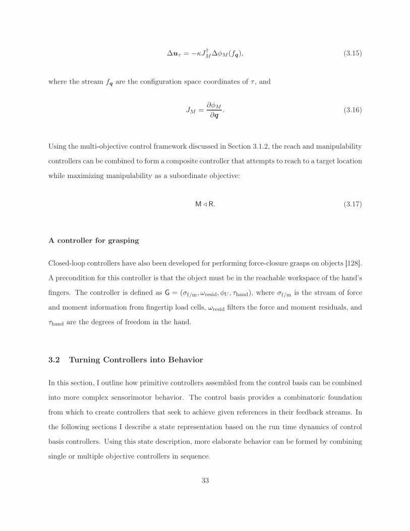
∆uτ = −κJ†M∆φM (fq), (3.15)

where the stream fq are the configuration space coordinates of τ , and

JM =∂φM

∂q. (3.16)

Using the multi-objective control framework discussed in Section 3.1.2, the reach and manipulability

controllers can be combined to form a composite controller that attempts to reach to a target location

while maximizing manipulability as a subordinate objective:

M ⊳ R. (3.17)

A controller for grasping

Closed-loop controllers have also been developed for performing force-closure grasps on objects [128].

A precondition for this controller is that the object must be in the reachable workspace of the hand’s

fingers. The controller is defined as G = (σf/m, ωresid, φU , τhand), where σf/m is the stream of force

and moment information from fingertip load cells, ωresid filters the force and moment residuals, and

τhand are the degrees of freedom in the hand.

3.2 Turning Controllers into Behavior

In this section, I outline how primitive controllers assembled from the control basis can be combined

into more complex sensorimotor behavior. The control basis provides a combinatoric foundation

from which to create controllers that seek to achieve given references in their feedback streams. In

the following sections I describe a state representation based on the run time dynamics of control

basis controllers. Using this state description, more elaborate behavior can be formed by combining

single or multiple objective controllers in sequence.

33

ǫ

φ

A

B

a

φ

Figure 3.3. The dynamics of two controller activations. The grey area, φ ≤ ǫ, represents the quies-cent state for the controller; when the dynamic state enters this region, the controller is consideredto be converged. Controller A has reached a quiescent state where φ = a. Controller B has not yetreached quiescence, but has already reached a lower absolute level of the artificial potential than A.

3.2.1 Discrete State Dynamics

A controller assembled under the control basis suppresses disturbances and acts teleologically to

achieve the goal state encoded in the artificial potential field. The dynamic response of the controller

provides a natural way to represent the state of the robot with respect to its desired objectives.

By classifying the response of a controller into a set of discrete states, the continuous, dynamic

behavior of the robot can be characterized by a discrete state space. This discrete-event dynamic

system (DEDS) representation of the control basis was first proposed by Huber [82].

The dynamic response of a closed-loop controller with a defined feedback signal can be described

in terms of the instantaneous state of the potential field (φ, φ) at time t. For asymptotically stable

controllers, φ is positive definite and φ is negative definite, so that the dynamic state (φ, φ) remains

in the lower right quadrant. Figure 3.3 shows the dynamic response of a closed-loop controller

reaching multiple attractor states. The controller is quiescent when φ < ǫ. The absolute level of

error in the controller when in a quiescent state is described by φ. The quantity φ represents the

observed, finite-difference time derivative of φ.

34

1

∅

∗

0

Figure 3.4. The quad state graph is a state machine describing the run-time dynamics of a controlbasis behavior. The starting state ∗ represents an undefined state in the underlying controller. Thestate ∅ denotes an undefined reference. The states 1 and 0 represent whether the controller hasconverged or not, respectively.

This description of the dynamics of controller state was used by Coelho to learn a model of robot

activity based on a history of task examples [29]. He derived a discrete state representation by

matching the run-time trajectory to a set of exemplar trajectories.

For a given controller Ci at time t, define the quadripartite convergence predicate Pt(Ci) that asserts

whether the state has been measured, the absence of the feedback signal, and the convergence status

of the controller:

Pt(Ci) =

∗ : φi state is unknown

∅ : φi has undefined reference

0 : |φi| > ǫ

1 : |φi| ≤ ǫ

, (3.18)

where φi denotes the value of the artificial potential at t, and ǫ is a positive constant. The state

∗ denotes that the status of the controller is unknown, and the state ∅ specifies that the reference

fσ,ω is not present in the feedback signal. Given the presence of the reference, then the states 0 and

1 denote whether the controller has reached quiescence. The transition dynamics between these

four states are shown in Figure 3.4.

35

3.2.2 Sensorimotor Behaviors

Given a controller, the convergence predicate P(·) provides a way to discretize its convergence status

over time. In this section I describe how sensorimotor behaviors can be constructed by choosing a

sequence of controllers to activate based on a state space constructed using the convergence predicate

function. The behavior is a description of how a sequence of controllers should be executed in order

to achieve convergence of a target controller.

Definition 3.2 (Sensorimotor Behavior). Define a sensorimotor behavior B as the tuple (C,Z,G,A,T , π)

consisting of a set of controllers C, a state space Z, a set of goals states G ⊂ Z, an action space

A, a state transition model T , and a policy π. Each controller C ∈ C is a primitive controller. The

action set consists of the controllers in C along with multi-objective combinations,

A = Ci⋃

Ci ⊳ Cj ⊳ · · · ⊳ Ck. (3.19)

Each state in z ∈ Z is described by the vector z = [P(C1) · · · P(CN )], where N = |C|.

The policy is a mapping from state vectors to controllers, π : Z → C, and determines the active

controller for a given state. The set of goal states is strict subset of Z, since a goal state corresponds

to a quiescence condition for some controller in C. Therefore, G excludes the state in which all of

the controllers take the value ∗. The goal state represents the convergence of a specified set of

controllers that represent the goal or intention of the behavior.

Search-Track

To make this discussion more concrete, consider some behaviors that have been developed for a hu-

manoid robot. Hart et al. describe how these behaviors can be derived using a staged developmental

process [77, 75, 76].

36

[∗ ∅] A = S, T

z = [P(S) P(T)]

Search

TrackTrack

Search

[∗ 0] [∗ 1][∗ ∗]

[0 ∗]

[1 ∗]

Track

Figure 3.5. The Search-Track behavior. If a tracking reference is not found when the behavior be-gins, it activates the Search controller. This controller runs until it has located a tracking reference,at which point the Track controller is activated to foveate on the target.

Consider a humanoid with an articulated vision system. The first behavior is known as “Search-

Track,” and consists of searching for a sensory stimulus and maintaining it in the center of the visual

plane. This behavior uses two controllers:

Search S = (φU , fsearch|τv, τv). This controls the vision system’s degrees of freedom τv using a

quadratic potential to achieve references provided by fsearch|τv. This feedback stream samples

“search” coordinates from a distribution p(Fτv ) over the coordinate frame of τv that describes

where interesting visual stimuli may be found.

Track T = (φU , fsat, τv). The feedback stream fsat = (σv, ωsat) filters out areas of highly saturated

color from the raw visual stream σv. Controller T drives τv such that the visual stimulus is in

the center of the visual plane.

Given this set of controllers, CST = S,T, the state space consists of all the possible values

[P(S) P(T)]. The goal set consists of all the states in which the tracking controller is converged,

G = [∗ 1]. The policy for the “Search-Track” behavior BST is shown in Figure 3.5. From the initial

state [∗ ∗], the robot executes the track controller T. If no sensory stimulus is available to track,

the behavior is in the [∗ ∅] state, and the robot initiates the search controller S. Once the search

controller has been activated, the robot servos the visual system to coordinates chosen according to

the distribution p(Fτv ). When S has converged on a search location, T is again activated. At some

point when a visual stimulus is present, the behavior reaches the [∗ 0] state signifying that T has

37

S ⊳ T

A = S ⊳ T

z = [P(S) P(T)]

S ⊳ T

[0 0] [0 1][∗ ∗]

S ⊳ T

[1 ∅]

[0 ∅] S ⊳ T

Figure 3.6. The Search-Track behavior using a multi-objective controller. In this instance, theSearch and Track controllers are co-activated, and they are prevented from destructively interferingby using null space projection.

a reference but has not yet converged. Once T has converged, the behavior reaches the goal state

[∗ 1].

If the multi-objective controller S⊳T is added to the action set, then an alternate form the behavior

can be defined, as shown in Figure 3.6. In this formulation, the robot executes S⊳T until completion.

3.2.3 Hierarchical Structure

The concept of a sensorimotor behavior can be extended hierarchically by allowing behaviors to be-

come sub-actions to other behaviors. Although each behavior is a temporally extended action, with

its own state, it can be abstracted into a single action by extending the convergence predicate (3.18)

for a behavior B as:

Pt(B) =

∗ : zt = [∗ · · · ∗]

∅ : zt = [∅ · · · ∅]

0 : otherwise

1 : zt ∈ G

. (3.20)

In the following section I describe a behavior that makes use of the Search-Track behavior as a

sub-action.

38

z = [P(BST) P(R) P(G)]

∅

∗

0

1

[1 ∗ ∗]

[∗ ∗ ∗] [∗ 0 ∅]

[∗ ∅ ∅]

Search-Track

R ⊳ G

R ⊳ G︷︸︸︷

R ⊳ G

[∗ 1 1][∗ 1 0][∗ 0 0]

A = S ⊳ T, R ⊳ G

Figure 3.7. The Reach-Grasp behavior can initiate the Search-Track behavior if a reaching targetis undefined. After Search-Track has found a target, the behavior executes the multi-objectiveReach controller subject to a Grasp controller.

Reach-Grasp

The ability to recognize objects of interest within the workspace is a prerequisite for manipulation

tasks. Thus, the Search-Track behavior provides a useful starting point for developing hierarchical

behaviors. By combining Search-Track with the Reach and Grasp controllers, one can construct a

hierarchical behavior that identifies and attempts to grasp objects of interest within the workspace.

This is the Reach-Grasp behavior BRG.

In this behavior, the set of controllers is CRG = BST,R,G, and the state vector is [P(BST) P(R) P(G)].

The goal state for this behavior has the grasp controller in the converged state. The Reach controller

is configured to use the same feedback element as the Search-Track controller, for example, fsat,

will identify objects that have highly saturated colors.

Figure 3.7 shows the policy for the Reach-Grasp behavior, which was learned from a process of

exploration and accommodation, detailed by Hart [76]. From the initial state, the robot assesses the

convergence of the multi-objective controller R⊳G. If the object stimulus is visible in the workspace,

then the behavior transitions to the state [∗ 0 ∅]. However, if no stimulus is immediately present,

39

the robot transitions to state [∗ ∅ ∅] and activates the Search-Track behavior BST. Once an object

stimulus has been found by Search-Track, the robot executes R⊳G to reach to and grasp the object.

3.3 Representing Complex Behavior with Schemas

In the preceding sections, I have outlined how closed-loop controllers can be composed in a program-

matic way using the control basis. These controllers are individual teleologic units of action that

achieve specified references, and they can be combined into more complex sensorimotor behaviors by

introducing a state space induced by the convergence predicate. In this section I describe sensorimo-

tor schemas: declarative abstractions of sensorimotor behaviors that admit multiple instantiations

into executable behavior using procedural resources induced by run-time constraints. The schema is

a generalization of the sensorimotor behavior described above, and requires decomposing controllers

into declarative and procedural components.

3.3.1 Declarative and Procedural Decomposition of Controllers

A controller Ci = (fi, φi, τi) can be decomposed into separate procedural and declarative specifi-

cations, p(Ci) and d(Ci), respectively. The procedural specification of the controller consist of the

feedback and effector resources allocated to the controller:

p(Ci) ≡ (fi, τi). (3.21)

The declarative type specification for the controller describes the artificial potential function, and

the coordinate frames of the feedback element and effector resource associated with the controller:

d(Ci) ≡ (φi,Ffi,Fτi

). (3.22)

40

The typing constraints of the declarative component define an equivalence class of controllers in the

control basis:

DA = Ci ∈ CB | d(Ci) = d(A). (3.23)

The set of controllers DA represent an abstract action that maintain the same declarative component

as controller A.

The procedural component, determined by run-time conditions, defines the topology of the artificial

potential function and the area of the robot’s workspace that may be affected by the controller. The

declarative component describes the type of coordinate system over which the potential is defined,

and the properties of the potential itself. The reach controller from Section 3.1.3, R = (fx, φU , τ),

can be decomposed into procedural and declarative components as follows:

p(R) = (fx, τ) (3.24)

d(R) = (φU ,Fx,Fτ ). (3.25)

3.3.2 Sensorimotor Schemas

A sensorimotor schema is a hierarchical, declarative control structure that is invariant to run-time

context. Each schema is a generalization of a behavior B, into declarative and procedural policies.

Definition 3.3 (Schema). A sensorimotor schema S is the tuple (C,Z,G,A, π, ψ). The components

of the schema are based on a behavior B. The set C is the set of controllers and or behaviors from

B, G ⊂ Z is the set of goal states, π is the action policy π : S → A, and ψ is the procedural policy

ψ : A× E → Σ × Ω × T , where E is the environmental context.

The state set is composed of convergence predicate vectors z = [P(d(C1)) . . .P(d(CN ))], for Ci ∈ C.

The abstract action set A is composed of the declarative components of C:

A = d(Ci) ∪ d(Bj). (3.26)

41

Because a schema is a declarative abstraction, it provides a way of representing teleologic behavior

across many different operating contexts and run-time conditions. The procedural components of the

controllers within a schema are determined by the robot at run-time based on the environmental

context E. In Chapter 5, I describe how probability distributions p(Σ,Ω | A, E) can be used to

represent this procedural policy.

Like the sensorimotor behaviors they generalize, schemas provide a hierarchical representation of

declarative knowledge. By allowing the use of sensorimotor behaviors as actions, the schema can

leverage and re-use previously acquired behaviors that address specific sensorimotor goals. Further-

more, the hierarchical structure allows for a more simple, abstract representation at the highest

level. Hart describes how schemas may be learned through a developmental, intrinsically motivated

learning process [76].

By executing the actions according to the transition model of the schema, the robot will act to

achieve the schema’s goal condition. The transition model may support a number of different paths

to a goal state. This allows the schema to represent different contingent behavior. The realized

path through the state space will depend on the run-time conditions experienced by the robot. For

example, the schema may have behavior for addressing various error states that may occur during

execution.

3.3.3 Pick-And-Place

In this thesis, I have focused on robot manipulation tasks that fall under the general description

of “pick and place” tasks [106, 89, 101]. These sorts of tasks require the robot to identify and

manipulate objects within its workspace. While the specifics of the pick and place behavior depend

on the run time environmental context, many common object manipulation tasks fall under this

description, such as sorting and stacking tasks.

At its most basic, the Pick-And-Place schema describes the actions of acquiring an object in the

workspace, transferring the object to a new location, and then releasing the object at that location.

42

R ⊳ P︷︸︸︷

∅

∗

0

1

A = R ⊳ G,R ⊳ P

z = [P(BRG) P(R) P(P)]

Reach-Grasp

[1 ∗ ∗] [∗ 0 ∅][∗ ∗ ∗] [∗ 0 0] [∗ 1 0] [∗ 1 1]

[∗ 0 1]

Figure 3.8. The Pick-And-Place Schema. The Reach-Grasp behavior is used to initially grasp theobject, and then the multi-objective Reach subject to Place controller is executed.

The first two steps can be achieved using the previously described Reach-Grasp behavior and Reach

controller, respectively. The final “placing” component requires the introduction of a new controller

to the robot’s repertoire. The Place controller P = (fnet, φU , τarm) is used to achieve a net force

reference for a grasped object by controlling the hand and arm resource τarm. It uses the quadratic

potential, along with the net force stimulus fnet = (σf/m, ωnet) that is derived from force/torque

sensors in the hand.

Let SPP be the pick and place schema. The set of behaviors in this schema is CPP = BRG,R,P. The

state vector z = [P(BRG) P(R) P(P)] is composed of convergence predicates for the Reach-Grasp,

Reach, and Place controllers. Figure 3.8 shows the state transition graph for Pick-And-Place.

On initialization, the robot attempts to acquire the object through the use of the Reach-Grasp

behavior. If it is successful, this puts the robot into the state [1 ∗ ∗]. From this state, the robot

executes the multi-objective controller R ⊳P in order to move the object to the correct goal location

and controls the reaction force of the object while releasing it. The schema reaches a goal state

when P(P) = 1, meaning that the place controller has converged.

The basic pick and place schema can be augmented by multiple contingencies, for example, error

recovery: if the object is inadvertently dropped by the manipulator prior to reaching the desired

location, the robot can regrasp the object and finish the original place phase. For bimanual hu-

43

manoids, the schema can also contain contingencies for the case of pick and place locations which

are reachable by different manipulators. In such a scenario, the robot must transfer the object

between manipulators to successfully complete the behavior.

3.4 Discussion

The control basis architecture presented in this chapter provides the robot with a way of creating,

representing, and reusing sensorimotor behaviors. The schema construct is a hierarchical way to

represent teleological behavior that can be decomposed into a general, static declarative component,

and the dynamic, procedural component that is applied at execution time using environmental

features.

In the following chapters, I describe my approach to PbD based on the assumption that the robot has

been endowed with a basic level of behavior competence. Sensorimotor schema constructed using

the control basis mechanisms provide a way to represent this behavioral competency. The question

of the origin of these behaviors is left to the individual designer. Although they may be designed

by hand, many of the behaviors described in this chapter have been learned via a developmental

learning process that incorporates intrinsic reward on multi-modal sensor input [76].

44

CHAPTER 4

A DECLARATIVE REPRESENTATION FOR PROGRAMMING BYDEMONSTRATION

The declarative aspect of a demonstration describes the task that is being observed as an abstraction

of states. As discussed in the Section 2.2.2, a common representational approach in the literature

is to focus on the trajectory of the demonstrator. In this chapter, I argue that trajectories are an

insufficient means for learning declarative knowledge from demonstration.

Trajectory-based approaches suffer from a lack of generalizable knowledge. A trajectory is valid

only for a given environmental context. Similar trajectories may serve drastically different task

objectives, and a large portion of the trajectory is typically not relevant to the task.

Instead, the robot should extract the intention of the demonstrator. Intention is a much more

powerful property of the demonstration that allows the robot to abstract out a specific run-time

context. The robot has a built in set of behaviors, outlined in Chapter 3, at its disposal. In this

chapter I describe how the robot can use statistical inference along with its own set of behavioral

schemata to interpret the information presented in a demonstration. The declarative information

encapsulated in the schema provide a framework for extracting intentions from the demonstration.

A demonstration session provides a continuous stream of high-bandwidth information to the ob-

server. Limited computational resources means that the robot must pick and choose which parts of

the demonstration merit full attention. While observing a teaching episode, the robot should extract

the relevant teaching cues from the sensor stream in order to create a compact representation of

the knowledge being expressed by the teacher. The teleological argument provides a motivation for

45

deciding which portions of the teaching signal require additional scrutiny: information associated

with end states should be inherently more interesting to the robot. The temporal structure of end

states, signaled by the convergence of a controller, can “explain” the intent of a demonstration.

When an end state is observed, the robot records and associates the reference of the converged

controller (and predicted schemas) with features that are spatially related to the reference. The

robot can later create a segmentation of feature space based on the features associated with end

states.

4.1 Declarative Representation of Schemas

The underlying process dynamics of a sensorimotor schema are described using a discrete set of

states defined by the convergence status of the constituent closed-loop controllers. In this chapter,

I describe how the robot can use this DEDS representation, along with a set of behavior schemata

to interpret the actions of a demonstrator.

By matching the demonstration to one of its internal models of behavior, the robot explains the

observed behavior using constructs it can use to recreate it. A further benefit of this approach is that

by representing the demonstration as a sequence of schema executions, when the robot attempts to

apply the knowledge gained from demonstration, it can use all of the knowledge embedded within

the schema—even if this was never observed in demonstration.

The schema matching process performs a type of behavioral quantization: the demonstrator’s behav-

ior is mapped onto prespecified declarative structures. In order to maximally capture the intention

of the demonstrator, the basis set of declarative schemas must span the space of behavior that the

robot is likely to observe.

Given a declarative specification, the robot uses the run time context to determine the appropriate

procedural details required to execute the schema. These procedural details include proper resource

allocation, and the identification of appropriate reference values for the underlying controllers. In

46

Chapter 5, I describe how the robot can create probabilistic models of procedural context for a

given schema conditioned on the run-time environment.

4.1.1 Hidden Markov Models

The Hidden Markov model (HMM) is an established method for representing a stochastic process

that exhibits serial dependence between observations [131]. These models have been used in a wide

variety of applications, including speech recognition [132], and have been used in PbD applica-

tions [158, 81, 2, 1]. In the following I will give a brief introduction to hidden Markov models.

Consider a sequential stochastic process observed over T time periods. Assume that at each time

period, the system is in an unobserved (hidden) state st, with the full state sequence given by

S = (s1, . . . , sT ). Each time period also has an observation xt, such that the full set of observations

is X = (x1, . . . , xT ). An HMM describes a joint probability distribution p(X,S) over the set of

states and observations.

In the HMM, the sequence of states has the Markov property, meaning that the distribution of the

current state given the previous state is conditionally independent of the rest of the state history:

p(st | s1, . . . , st−1) = p(st | st−1). (4.1)

Furthermore, the current observation depends only on the current state:

p(xt | s1, . . . , st) = p(xt | st). (4.2)

The sequential stochastic process given by the distributions (4.1) and (4.2) describe a type of

dynamic Bayesian network [131, 40]. This model is shown in graphical form in Figure 4.1. A

graphical model uses a graph to represent a conditional probability distribution. The nodes in

the graph are random variables and edges represent conditional probability relationships between

variables.

47

xt−1 xt xt+1

st+1stst−1

Figure 4.1. The Hidden Markov Model. The grey nodes are observed variables. At each time step,an observation is generated conditional on the latent variable. The next state variable is chosenfrom a distribution conditioned on the value of the current state.

The HMM is a generative representation of the stochastic process. A generative model is one that

represents a joint probability distribution such that one may sample the modeled parameter.

The distribution (4.1) describes the likelihood of the system moving from one state to another. For

each step in the chain, the next state is given by a distribution that takes a parameter θst dependent

on the state st:

st+1 | st ∼ p(st+1 | θst), (4.3)

and a distribution over the set of initial states:

s1 ∼ p(π). (4.4)

The set of parameters θ = θi and π describe the transition model for the process. If the full

sequence of states is known, then its probability given a transition model is computed as

p(S |θ) = p(s1 |π)T∏

t=2

p(st | θst−1). (4.5)

At each time step, the system generates an observation according to the distribution (4.2):

xt | st ∼ p(xt | ξst), (4.6)

48

where ξ = ξi is the set of parameters that make up the observation model of the system. The

probability of a sequence of observations generated from a known set of states is given by

p(X |S, ξ) =

T∏

t=1

p(xt | ξst), (4.7)

reflecting the conditional independence of observations on the state from which they were observed.

The joint distribution of the observations and states is described by

p(X,S |θ, ξ, π) = p(X |S, ξ) p(S |π,θ) (4.8)

= p(s1 |π) p(x1 | ξs1)

T∏

t=2

p(xt | ξst) p(st | θst−1). (4.9)

The HMM model H = (π,θ, ξ) is the tuple of parameters that make up the transition and observa-

tion models.

When trying to apply these models to real world processes, the goal is to identify the model H′ ∈

Hi that is most likely to have generated a sequence of observations X.

H′ = argmaxHi

p(Hi |X). (4.10)

The model H′ is the maximum a posteriori (MAP) model, since (4.10) maximizes the posterior

distribution p(Hi |X) given by Bayes’ theorem,

p(Hi |X) =p(X |Hi)p(Hi)

p(X). (4.11)

The likelihood term of (4.11) can be found by integrating over the entire state space,

p(X |Hi) =

∫

Sp(X |S,Hi) p(S |Hi)dS. (4.12)

Naively computing (4.12) by iterating over every possible state sequence S ∈ S quickly becomes

intractable as the number of observations grows. However, there exists a more efficient dynamic

49

programming procedure known as the forward-backward method for computing this quantity in time

O(|S|2T ) [11].

The estimation problem for an HMM attempts to find the model parameters Hi with maximum

likelihood for a given observation sequence,

maxHi

p(X |Hi) = maxHi

∫

Sp(X,S |Hi). (4.13)

The Baum-Welch method is a well-known expectation-maximization algorithm for finding a local

maximum of (4.13) [12, 42].

Example: HMMs for speech recognition

Hidden Markov models have been used with great success in the domain of speech recognition [131,

93]. In a typical application, the audio signal is broken into overlapping windows of 50 ms, spaced

30 ms apart [93]. Although the speech signal is nonstationary, the assumption is that at the

short time scale of an individual window, the signal can be considered to a sample from stationary

stochastic process. A feature vector is computed over each window in order to generate a more

compact representation of the spectral properties of the window. Each feature vector is a single

observation xt, and the entire signal is represented as a sequence of observations X = (x1, . . . , xT ).

The unobserved state st represents a stochastic process capable of generating short time scale

spectral observations—each state is an individual speech phoneme. The latent state sequence

S = (s1, . . . , st) represents a temporal relationship among the different phonemes. The HMM pro-

vides a way to model temporal relationships between these processes based on short term spectral

observations.

In a system for single word recognition using HMMs, assume there is a vocabulary of W words to be

recognized. Furthermore, assumed there are L labeled examples of each word, spoken by multiple

speakers. The following steps are used to perform the recognition:

50

1. Using the Baum-Welch algorithm, build an HMM model Hw for each word in the vocabulary,

1 ≤ w ≤W , using the observations from the L examples of each word.

2. Given a set of observations X for an unknown word, compute the likelihood of each of the W

models, p(X |Hw) using the forward-backward algorithm.

3. From the set of W likelihoods computed in the previous step, choose the word w∗ whose model

has maximum likelihood:

w∗ = argmax1≤w≤W

p(X |Hw).

4.2 Interpreting Demonstration

In my approach to PbD, I assume that the observing robot has a set of sensorimotor schemas S. The

demonstration is viewed as a realization of a sequential stochastic process. I model the underlying

process as an instantiation of a sensorimotor schema, and the robot must infer which schema S ∈ S

is most likely to generate the observed actions. Taking a similar approach to speech recognition,

I associate an HMM HS with each schema S ∈ S. If HMM HS′ is the most likely model given

the observations, then schema S′ is considered to “explain” the demonstration. By abstracting the

demonstration in terms of a schema, the robot has implicitly assigned a teleological goal to the

demonstration that is addressed by the schema.

I will first present a simplified model of demonstration that assumes that each demonstration can

be represented by a single schema instantiation. Later in this chapter I describe how this constraint

may be relaxed.

Let schema S ∈ S consist of a set of states Z and actions A. Each state z ∈ Z is a vector of

convergence predicates

z = [P(d(C1)) . . .P(d(Cn))] . (4.14)

51

A monitor is a special type of controller defined with no effector resource: C = (σ, ω, φ,∅). A

monitor lacks the ability to effect the environment; instead, it updates its potential function based

on the actions of other controllers.

For each abstract action d(Ci) in S, one can define a monitor set:

M(Ci) = Cj | d(Cj) = d(Ci). (4.15)

Each element of M(Ci) is a monitor with a different feedback reference. Consider a schema that

contains the abstracted version of the search-track controller, S ⊳T. The monitor set M(S ⊳ T) con-

tains multiple instantiations of search-track, each with a different stimulus reference. For example,

a monitor set can be constructed using the saturated pixel blob feedback reference, fsat, and the

motion area reference, fmotion:

M(S ⊳ T) = S(fsat) ⊳ T(fsat),S(fmotion) ⊳ T(fmotion), . . .. (4.16)

For the purposes of observing a demonstration, the robot should have as many monitor instantiations

per abstract action as possible, to span the space of possible stimuli that may be generated by the

demonstrator. Like mirror neurons, those neurological structures that respond to both executing

and observing certain types of actions, monitors allow behavior-producing schemas to be used to

observe behavior. By associating an HMM with each schema, the robot can identify the schema

most consistent with the demonstration.

Controller convergence can be evaluated in a monitor: convergence denotes whether the state of the

robot is such that the controller would be converged if it were actuating the robot.

The convergence status of a monitor set is an operator on the elements of the monitor set M (Ci):

P′(M(Ci)) =

0 : if all P(Mk(Ci)) = 0

1 : if any P(Mk(Ci)) = 1. (4.17)

52

If the robot observes a goal condition for an instantiation of the abstract action, then a monitor in

the set will be in a converged state.

Prior to beginning the demonstration, the robot creates monitor sets from the controllers in the

union of the abstract actions represented in its universe of schemas S. Let M represent all the

instantiated monitors:

M =⋃

Ci∈S

M (Ci). (4.18)

At each time step in the demonstration, the robot constructs a single observation vector that consists

of the convergence status of all monitor sets in M:

xt = [P′(M 1(Ci)) . . .P′(MK(Ci))], M j(Ci) ∈ M. (4.19)

The observation vector has size K = |M|, where K is the number of distinct abstract actions in the

robot’s universe of schemas. The organization of abstract actions into a single observation vector is

shown in Figure 4.2.

In order to evaluate the likelihood of each HMM HS, it is necessary to define each HMM’s observation

and transition models. For schema S, the transition parameters come from T , the transition model

of the schema, such that θ = T . Since the schema’s state space is discrete, a multinomial distribution

can be used to model the transition probabilities between states:

st+1 | st ∼ Multinomial(st+1 | θst). (4.20)

The observation model of HS is a distribution over xt given a latent state, p(xt | ξst). Because

xt consists of all the unique abstract actions in the robot’s universe, each schema’s state vector is

composed of a subset of the abstract actions in xt. Therefore, it is possible to evaluate the likelihood

53

xt = [

φ

P′(M(Ck))

φ

φ

P′(M(Cj))

M(Cj)M(Ci)

φ

φ

]P′(M(Ci))

M(Ck)

φ

φ

φ

φ

φ

φ

φ

φφ

ǫ

φ

ǫ

φ

φφ

ǫ

Figure 4.2. The organization of monitors into an observation vector. In this figure, there arethree monitor sets for controllers i, j, and k. Each monitor set consists of a group of monitorswith different controller references. The state variable xt is composed of the concatenation of theconvergence status of each monitor set.

of each schema’s observation model given xt. Each state in a schema is defined by the convergence

status of the underlying abstract actions in that schema. Therefore, state st can be considered a

likely state for xt if the abstract actions in st have the same convergence values in xt. This is

represented in the following distribution:

p(xt | st) =∑

x | st=x

δx, (4.21)

where δx is a Dirac delta function at x. The atoms x are the realizations of the observation vector

that have the same convergence status as the abstract actions in st.

After T time steps, the robot has a set of observations x = [x1 . . .xT ], and can compute the

most likely schema by maximizing the posterior distribution p(HS′ |x) using (4.21), (4.20), and the

forward algorithm.

The robot also keeps a history of which monitors within each monitor set have converged, so that

it can build a procedural model of the demonstration as well. This allows the robot to track which

procedural details are being demonstrated by the teacher. The feedback elements of M(Ci) that are

converged provide information on the procedural elements of the demonstration. Knowing which

54

feedback elements elicited a converged response during the demonstration allows the robot to build

a procedural policy ψS′ for the inferred schema. The procedural policy determines the effector

resources allocated to the schema based on the environment and preferences at run-time.

A further benefit of this approach is that the robot can use the state transition model T of the

inferred MAP schema S′ to estimate which controllers may be activated next.

4.3 Applying Knowledge from Demonstration

After observing a demonstration, the robot infers the most likely schema that explains its observa-

tions. Given the declarative structure of this schema, the robot forms a procedural model for the

schema based on the features exhibited by the demonstrator. Once the robot has acquired a declar-

ative and procedural model, it can apply the knowledge learned from demonstration to new task

instances. In this section I outline an experimental validation of the declarative inference process

outlined above.

4.3.1 Experimental Apparatus

The experimental platform used in this dissertation is Dexter, the UMass bimanual humanoid,

shown in Figure 4.3. Dexter has two manipulators—Barrett Technology’s Whole-Arm Manipulator

(WAM)— arranged in an anthropomorphic configuration. Each WAM has seven degrees of freedom

with a cable transmission and direct drive motors. Additionally, each WAM is equipped with a

three-fingered hand, also manufactured by Barrett, that feature six-axis force/torque load sensors

on the fingertips. Dexter has a stereoscopic vision system comprised of a shoulder-mounted pan tilt

unit with four degrees of freedom (pan, tilt, and independent vergence for each camera).

The teleoperation system uses glove-based controller worn by the operator. The glove is augmented

with IR LEDs that are triangulated by a base unit. This allows the system to detect six degrees

of motion of the teleoperator’s hand. Further, the glove also measures finger flexion of all five

55

Figure 4.3. Each of Dexter’s arms has 7 DOF and is equipped with a three-fingered hand withfour total degrees of freedom. The stereo head has four degrees of freedom.

fingers. Although Dexter has a stereo pair of cameras, the wide baseline between the cameras

makes natural 3D video awkward for a teleoperator. Therefore, Dexter has a second stereo pair

of video cameras with a narrower baseline mounted on Dexter’s chassis under the shoulders. This

allows the teleoperator to have a 3D view of Dexter’s workspace.

4.3.2 Experiment: A sorting task

For experimental validation of the declarative inference process outlined above, a pick and place

task was demonstrated to Dexter. In this task, orange and blue objects were placed on the table in

front of the robot. Two containers were placed behind the objects. The task was to place the orange

objects into the right bucket, and the blue objects into the left bucket. In order to demonstrate the

task, the teacher teleoperated Dexter’s right arm, τx,r, and placed the orange object in the right

bin, and the blue object in the left bin.

Figure 4.4 shows a screen grab of the video feed used by the demonstrator. The teleoperator has the

option of viewing the scene in 3D using a red/blue stereo feed. The traffic light icon in the top right

56

Figure 4.4. The teleoperator’s viewpoint. The icon in the upper right denotes whether theteleoperator is actively controlling the robot. The graph in the upper-left denotes the convergencestatus of the active schema. The red circle denotes the current state, while the dark red circles arepreviously visited states.

indicates when the teleoperator is actively controlling Dexter. The graph icon in the upper left of

the frame is a representation of the robot’s current inferential state. Each of the nodes represent a

different state in the pick and place schema. Nodes colored gray are unvisited, dark red nodes are

visited states, while the bright red node represents the current state.

After observing this demonstration, Dexter can infer the most likely declarative schema using (4.13).

For this task, H′ = SPP, the pick and place schema. In Chapter 5 I describe how the robot infers a

procedural model for the schema SPP given the observed task. This model, MPP, associates features

of the objects in the task with the feedback elements of the controllers in SPP.

Give the declarative model SPP and the corresponding procedural model MPP, the robot can apply

the knowledge learned in demonstration to new task instances. After demonstration, Dexter is

57

Figure 4.5. A sorting sequence, clockwise from top left. The sorting task is to place orange objectsin the right bin, and blue objects in the other. The original demonstration used Dexter’s right armand bins in different locations. In this execution, Dexter autonomously uses its left arm to sort theball into the left bin.

presented with objects and applies the knowledge from demonstration to place the objects into the

appropriate buckets.

Once the pick-and-place schema has been identified as the “source” of the observations in the demon-

stration, the robot can leverage all the sensorimotor knowledge present in the schema. The schema

encapsulates a policy for resource allocation based on environmental context. Figure 4.5 shows a

sequence of video frames showing Dexter sort a blue object. Note that Dexter uses its left arm,

τx,l to perform this task, even though the teleoperator only performed the demonstration using the

right arm. In this case, the pick-and-place procedural policy ψPP identified the left arm as necessary

for executing the schema instance given the location of the blue ball.

58

Figure 4.6. A sorting sequence, clockwise from top left. In this execution, the robot must sort the orange object into the rightbin. This requires transferring the object between the workspaces of the two arms. This illustrates the contigency event of armto arm transfer in the Pick-And-Place schema.

59

Figure 4.6 shows another sequence of video frames where Dexter uses both arms to place the orange

ball in the right bin. Dexter first grasps the ball using its left hand and places it on the table in

the workspace of the right hand. After this, Dexter grasps the object with its right hand and places

it in the bin. The pick-and-place schema SPP has a contingency for performing this type of hand

to hand transfer. Although this type of transfer was never performed by the demonstrator, since

Dexter uses SPP as a declarative representation of the demonstrated task, it can use any of the

sensorimotor behavior contingencies available in the schema.

The declarative schema provides a teleological representation of the demonstration: the schema

describes a state machine for achieving a behavioral goal. The schema is an abstract representation

of the task, and the procedural policy allows Dexter to execute the schema in a variety of settings.

Although the teacher may have provided a limited set of procedural examples, the procedural policy

associated with the schema allows Dexter to generalize the demonstration to novel settings. The

important aspect of the demonstration that must be extracted is what is the declarative goal—

represented by the schema—and what are the necessary procedural details associated with closed-

loop controller references used by the schema.

4.3.3 Discussion

The experiment discussed in this section provides a proof of concept of the declarative inference

architecture presented in this chapter. Although the experiment is limited in scale, it shows the

power of leveraging the schematic representation of demonstration. The robot is able to apply a

range of knowledge that it has acquired to perform the task, even if that particular behavior was

not demonstrated.

I described how the robot can assign a single schema as “responsible” for the observed demonstration.

It is possible to extend this architecture hierarchically in order to describe tasks as sequences of

schema executions. The hierarchical HMM is an abstraction of the HMM model that allows for

60

multiple levels of latent variables [23]. Using hierarchical HMMs, one can assign separate schema

invocations to different portions of a single demonstration.

61

CHAPTER 5

PROCEDURAL INFORMATION FROM DEMONSTRATION

In previous chapters, I have discussed a declarative representational framework that the robot uses to

represent and infer sensorimotor behavior. The sensorimotor schema defined in Chapter 3 contains

a procedural policy:

ψ : A× E → Σ × Ω × T (5.1)

that maps abstract actions and environmental conditions to the procedural assignment for a con-

troller: the appropriate feedback element (Σ × Ω) and effector resource (T ). The environmental

context E consists of observed features and any task identifying information provided by the demon-

strator, E = (G, t).

In this chapter I introduce methods for inferring procedural policies from demonstration. I represent

these policies using a generative, probabilistic approach. I take a Bayesian approach, by building

models that fully leverage the robot’s prior knowledge. Another benefit of the approach is that the

robot can refine its model iteratively as new data becomes available. This is particularly useful in

PbD tasks, as it allows the teacher to evaluate the robot’s performance of the target task and reduce

unnecessary training examples. Furthermore, prior information is useful in the inference process

when observations are sparse.

The task is an assignment of value to certain states of the world by the demonstrator. The actual

states and values are latent to the robot, and the purpose of the demonstration is to provide examples

of states with high value. The perceptual features in the demonstration provide information on how

the robot can identify high value states.

62

Skill transfer is a term used to describe the ability of the robot to generalize concepts from one task

instance to another. In this case, demonstration provides the information used to infer parameters

for a probabilistic model. This model allows the robot to account for uncertainty in the training

signal, and provides for generalization of the teaching patterns used by the demonstrator. The

probability distribution represented by the model is used to evaluate the utility of actions under

new operating contexts. The robot forms a policy using this measure of utility.

In the previous chapter, I described how the robot could infer a declarative “explanation” of the

demonstration in the form of a sensorimotor schema. The schema provides a roadmap for identifying

important features in the demonstration. These are features associated with the goal states of

the controllers within the schema. The procedural policy is responsible for selecting the feedback

elements and effector resources required to execute a schema, conditioned on the features in the

environment.

The robot is awash in sensory feedback from the demonstration, and the schema provides a way

to focus computational resources on the sensory information that provides the most information

relevant to the task begin demonstrated. By using a schema mechanism to abstract the actions

performed by a demonstrator, the robot is reducing the computational load during the observation

phase, and disregarding information that is not relevant to successful completion of the task. Fur-

thermore, The robot can use the knowledge it has been given up-front—sensorimotor schemas with

generative Bayesian models of procedural context—to reduce the amount of instruction required to

teach new task concepts.

In the remainder of this chapter, I describe how to represent the environment context used in

the procedural policy, and how to extract it from the run-time sensor stream. Then I discuss a

probabilistic model that relates features in the environment to the procedural context required for

schema execution. I examine in detail the example of the pick and place schema, and describe

a feature model for that task. Then I discuss the results of experiments using that model for a

63

sequence of pick and place tasks. I also discuss how the generative, Bayesian approach used by the

model can improve demonstration performance and assist in incremental learning.

5.1 Generative Models for Procedural Policies

As described in Chapter 3, the procedural parameters of schema S are those that depend on the

context in which the schema is executed. While the declarative structure of the schema determines

the type and order of controllers that are executed, the procedural context specifies the run-time

goals that are used to generate motions in each controller in the schema. These parameters are the

feedback elements and resource allocations for the underlying closed-loop controllers in the schema.

A single schema may have multiple abstract actions, each requiring different feedback and effector

resources. Let AS = a1, . . . , an be the abstract actions in schema S, RS = r1, . . . , rn be control

basis feedback elements ri = (σi, ωi), and TS = τ1, . . . , τn be the effector resources for S. In order

to execute S, the schema must be proceduralized by selecting sets RS and TS to provide feedback

and effector resources.

The types of feedback elements and effector resources that are used to proceduralize a schema depend

on the abstract actions in the schema and the environmental context in which the schema is to be

executed. Furthermore, there is a dependence between the abstract actions within the schema,

and for most schemas, the robot can not proceduralize each abstract action independently. For

example, in the pick and place schema, the proceduralization of the abstract place action depends

on the proceduralization of the preceding pick action.

Therefore, I represent the procedural policy as a joint distribution

ψ(S,E) = p(a1, . . . , an, r1, . . . , rn, τ1, . . . , τn, E) (5.2)

= p(AS , RS , TS , E) (5.3)

Given the schema and environmental context, the policy can be written using Bayes’ theorem as

64

p(RS , TS |AS , E) =p(AS , E |RS , TS) p(RS , TS)

p(AS , E). (5.4)

The identity of the schema S is inferred using the declarative inference described in Chapter 4.

The declarative state transitions in the schema identified using the HMM model provide the robot

with intermediate, teleological landmarks: end states of the constituent controllers in the schema. In

this chapter, I describe a generative, Bayesian probability model the robot infers from demonstration

to provide a procedural policy of the task.

I chose to use a generative, Bayesian feature model because it has properties that help reduce the

amount of demonstration required for concept learning. Generative and discriminative approaches

represent two different ways of modeling machine learning tasks. It has been shown that asymptot-

ically, as more data is acquired, a discriminative model will outperform a generative one. However,

if data is sparse, as in the case of programming by demonstration, a generative approach tends to

perform better [123].

The Bayesian approach offers the benefit of being able to apply prior knowledge to the model.

Prior information informs the model and allows for more successful generalization with less data.

The number of demonstrations required to teach a task or concept can used as a metric for the

effectiveness of the learner. The fewer the examples required, or the shorter the demonstration

session, the more quickly the robot can begin to apply that knowledge to new contexts. Furthermore,

demonstration can be tiresome and costly for the teacher.

In this chapter, I assume that the demonstration consists of exchangeable examples of a single

schema. Exchangeability is the condition that the joint distribution of the observations is invariant

to the ordering of the data. In this case, exchangeability implies that the order in which the demon-

strator provides training examples does not affect the task being demonstrated. If exchangeability

of training examples is not appropriate, or if the task requires multiple types of schema to be used,

then a more general hierarchical model can be used. As mentioned in Chapter 4, if the demonstra-

tion is represented using a sequence of schemas, then a hierarchical HMM can be used. In addition,

65

r2

r

n

K

θ

o

β

γq

x

K

r2

r

x

K

Figure 5.1. The simpler pick and place model used in this chapter. This model describes a singleinstantiation of pick and place.

there are T task variations; each variation uses different conditions for choosing references required

by the schema.

5.1.1 A Generative Model for Pick and Place Proceduralization

From the definition of the pick and place schema in Chapter 3, there are three abstract actions,

the reach-grasp behavior, BRG, the reach controller R, and the place controller P, that must be

proceduralized for the schema to be executed. The procedural policy must find a mapping from

the observed features and task context (G, t) to elements in the control basis for feedback elements

RS = rBRG, rR, rP and effector resources TS = τBRG

, τR, τP.

In this section, I focus on a special case of pick and place that describes a rich collections of behaviors

like sorting tasks. I assume there is a single, latent feature category q associated with each “place,”

meaning the destination of the object after being grasped. This category abstracts the notion of the

“place” destination for the controller. Given this category, the robot can proceduralize the actions

in the schema.

66

For each set of demonstration examples, the task parameters are the same, so that the number of

potential “places” for objects is fixed atK. Let Xt = x1, . . . , xK, xi ∈ R6, be the Cartesian position

and orientation of these targets that parameterize feedback elements ri where ri = (σx(xi), ωi).

In these experiments, I inform the robot of these locations prior to demonstration, but they could

be inferred from demonstration using techniques similar to those used for inferring pick targets,

described below.

In the PbD framework, the robot observes demonstrations and infers a model from those observa-

tions. Because a generative model describes the joint distribution of the observations and underly-

ing variables, one can describe the stochastic process from the other causal direction. That is, the

generative model describes a process for generating data observations by sampling from the joint

distribution.

The generative process for a single pick and place demonstration with n feature observations is show

graphically by Figure 5.1, and outlined in the steps below:

q ∼ Multinomial(ψ) (5.5)

rP | q = k ∼ δr(k) (5.6)

τP | rP ∼ δτ (rP) (5.7)

oi | q = k, 1 ≤ i ≤ n ∼ p(oi | θk). (5.8)

First, in (5.5), the latent place category q ∈ 1, . . . ,K is chosen using a multinomial distribution

over K elements with parameters ψ = (π1, . . . , πK−1), πK =∑K−1

i=1 πi. These parameters are the

probabilities for each distinct value 1, . . . ,K. For this sorting task, this distribution implies that

the frequency with which a class is presented in demonstration affects the likelihood of assigning

that class to a novel object. While this may be true for some tasks, in these experiments, I assume

that the teacher selects exemplars based on how well they reflect the class criteria to which they

belong, and not based on frequency of occurrence. Thus for the two-class case, if the demonstration

provides two examples of class 1, and one example of class 2, it does not mean that class 1 is twice

67

as likely as class 2. Therefore, I assign ψ a uniform distribution, signifying that each class is equally

likely a priori.

The remaining steps in the process reflect the dependence of the place location and observed features

on the value of q. The feedback element for the place controller is sampled in (5.6); based on this

selection, the effector resource is chosen in (5.7). The final step is to sample the feature data. Since

there is a single feature type in this model, and individual feature observation oi is sampled from

the distribution p(oi | θk), where the parameters of the distribution θk are specific to the category

q = k.

The exact form of the observation likelihood model, p(oi | θk), will depend on the type of feature

being used, and may be discrete or continuous distributions. In these experiments, visual features

are computed using a background subtraction routine to segment objects in the workspace. Fur-

thermore, these experiments use a discrete feature based on the color of the object being grasped,

and a continuous feature representing the size of the segmented object in pixels.

The feedback and effector resources for the reach-grasp behavior representing the “pick” action,

rBRGand τBRG

, can also be modeled using a latent category variable. However, for this type of

demonstration, the robot must predict the place category for a given object presentation, the pick

elements are known. In Chapter 6, I discuss how the robot can select a unique grasp affordance

preshape (and hence rBRG) based on visual features of the object.

The process outlined in (5.5)–(5.8) describes a model for a single execution of pick and place, and

generates a vector o of n observations and a single category assignment, q. Let D = (O,Q) where

O = o1, . . . ,oM and Q = q1, . . . , qM be the collection of observed and latent features from a

demonstration of M pick and place executions.

The purpose of the training session is to provide the robot with data it can use to infer parameters of

its feature model. It uses this model to decide the most likely “place” reference of an object presented

68

to the robot. The robot can also make a decision about whether the object should be manipulated

at all, based on the objects presented in the demonstration; this is discussed in Section 5.1.3.

After demonstration, in the execution phase, when a new object is presented the robot observes

features o and selects the most likely place category using a maximum a posteriori (MAP) estimate:

q∗ = argmaxq∈K

p(q | o,D), (5.9)

where, by Bayes’ theorem

p(q | o,D) ∝ p(o | q,D) p(q | D). (5.10)

The distributions on the right side of the equation incorporate the training data. Using q∗, (5.6)

and (5.7), the robot can proceduralize and execute the pick and place schema.

The procedure for computing (5.10) will differ based on the likelihood model learned from demon-

stration:

p(o | q,D) =

n∏

i=1

p(oi | θq). (5.11)

The right hand side of (5.11) illustrates the exchangeability assumption of the feature data: the

n feature observations are conditionally independent given the place category. Furthermore, the

likelihood function depends on the type of model represented by θq. If conjugate priors are used,

then one can compute efficient closed-form solutions for (5.11) that integrate out the parameters θq.

The second term on the right of (5.10) is a posterior distribution over place categories. If ψ is a

multinomial prior over q with a symmetric Dirichlet prior with parameter β, then the standard form

is:

69

p(q | D, β) = p(q |q, β) (5.12)

p(q = l |q, β) = Md(q = l |q, β, n = 1) (5.13)

=#q

l + β

(∑K

l′=1 #ql′) +Mβ

, (5.14)

where (5.12) follows from the independence relations in Figure 5.1. The symbol #ql denotes the

number of occurrences of the value l in the observation vector q. As mentioned above, for many

types of sorting tasks, this is a uniform distribution.

5.1.2 Experiments with a Sorting Task Using Pick and Place

As a motivating example to provide a basis for a more generalized probability model, in this section

I present examples of an object sorting task that utilizes the pick and place schema. In each task

instance, the concept to be learned is a two-class sorting rule for objects placed in front of the robot.

Prior to each demonstration session, the teacher selects a sorting criteria, and the demonstration

consists of examples from each class. For demonstration, an object is presented to the robot, and

the teleoperator uses Dexter to grasp the object and place it into one of K locations. In this section,

I use a batch learning approach, where the robot is presented with every demonstrated example

prior to performing the model inference and testing the learned model. In Section 5.2 I discuss an

incremental approach to this task.

After the demonstration, the robot enters the execution phase of the experiment. The user places

an object in the robot’s workspace, and using the feature model learned from demonstration, the

robot proceduralizes and executes a pick and place schema to place the object in a location.

The objects used in these experiments are shown in Appendix B. The objects are human-scale

objects that are present in a household environment. Because the robot does not model the iden-

tity of the objects, the same object presented in multiple orientations will appear as multiple task

examples. The robot computes the visual features of the presented object using background sub-

traction for segmentation and makes a classification decision using the feature model it inferred from

70

demonstration. In total there are 30 distinct objects in the dataset, with many objects presented

in multiple orientations, giving a total of 108 different object presentations.

To illustrate the model, I perform two sets of experiments, using a different feature type in each

set. In the first set of experiments, a discrete color feature is the sorting criteria. Each object’s

color classification is labeled by hand; the objects in each color class, along with color histograms,

are shown in Appendix B, Figures B.1–B.4.

To illustrate the use of a continuous feature variable, in the second set of experiments the size of the

object’s segment in pixels is the classification criterion. Again, each of the 108 object presentations

is labeled discretely as belonging to a Small, Medium, or Large category. This classification is shown

in Appendix B, Figures B.5–B.7.

Sorting based on color

In the training phase of these experiments, the robot is provided with M examples of each of two

color categories. The color feature is computed by associating one of L = 64 colors with each pixel

in the object segment. The discrete set of L colors is formed by a uniform partition of HSV space.

The histogram of colors is sorted in descending order, and the colors in the 20th percentile and

higher are included in the feature vector. The 20th percentile boundary helps to reduce noise in the

feature vector. Since the number of colors in the object segment varies for each object, the length

of the feature vector om may vary for each object m.

Given this feature, it is necessary to define the observation likelihood model (5.8). Since each

observation can take one of L different values, I use a multinomial distribution over oi with parameter

ψ = θk. Since this parameter also must be inferred from the data, I use a symmetric Dirichlet

distribution with parameter γ as a prior over θk, because the Dirichlet is conjugate to the multinomial

distribution. This allows the posterior over θk to be specified as a multinomial distribution.

71

As shown in Figure 5.1, there are K distinct multinomial distributions in the model; one for each

place category. Given the training set D = (O,Q), the inference problem is to compute the posterior

for each θk. One can rewrite (5.10) using this model:

p(q = l | o,D, γ) ∝ p(o | q = l,O, γ) p(q = l | D) (5.15)

p(o | q,O, γ) =

n∏

i=1

p(oi | q = l,O, γ) (5.16)

=

n∏

i=1

Md(oi | θ = (ol, γ), n = 1) (5.17)

=#O

l + γ

(∑L

l′=1 #Ol′ ) + kγ

. (5.18)

Using this form, the discrete feature model can handle any feature type that can be modeled by

a multinomial distribution. The resulting distribution (5.18) computes the posterior probability

by using a smoothed counting method, where the Dirichlet prior hyperparameter, γ, controls the

amount of smoothing. The total number of parameters in this model is linear in the number of

place categories.

Using the above model the robot infers the posterior over each θk by incorporating all 2M demon-

strations. In the execution phase, the remainder of the objects in each category are presented to

the robot, and the bin into which the objects are sorted is recorded.

Figure 5.2 shows the success rate (the number of correctly sorted objects divided by the total

number of objects presented) for sorting between Red and Blue classes. There are 24 Red object

presentations and 18 Blue presentations, so if n = 1, then one Red and one Blue presentation is

demonstrated to the robot, and the other 40 presentations are used to test the model. The objects

in each color class, along their color histograms are shown in Appendix B, Figures B.1–B.4.

Figure 5.2 shows the results of performing 10 different trials for each value of n, with error bars

indicating one standard deviation. As one might expect, the success rate increases as the number of

examples increases. However, the model is effective even with a single example of each color class.

72

1 2 3 4 5 60

0.1

0.2

0.3

0.4

0.5

0.6

0.7

0.8

0.9

1Success Rate for Place Location (red−blue)

Number of Examples

Suc

cess

Rat

e

Figure 5.2. This plot shows the success rate for sorting objects across 10 trials for each numberof example objects.

To determine the statistical significance of the sorting model, I compute a p-value using a χ2 test

for each of the 10 trials. Figure 5.3 graphs the maximum and median p-value computed for each

value of n. The dot–dash and dashed lines indicate 5 % and 1 % significance levels, respectively.

The graph shows that in most cases the results are significant. However, for small values of n there

were a few trials with less than significant sorting performance. This can be explained by the choice

of feature model.

By using a multinomial distribution to model the color feature, the robot is susceptible to noisy

training data. The multinomial is a frequency distribution for each color; the implication of this is

that the probability assigned to color a does not affect the probability of color b, even if a and b

are close together in color space. Therefore, if the training data contains colors that are not present

in the test data, then classification performance will suffer. Thus, the poor trials in Figure 5.3 are

the result of demonstration data that did not reflect the color values that would be seen in testing.

To get an idea of how well the objects in the Red classification shared similar colors, I compiled

Table 5.1.2. A bullet (•) at entry (i, j) indicates the robot can successfully sort object j if object

i is the only example provided. The table shows that most objects provide a sufficient range of

73

1 2 3 4 5 610

−4

10−3

10−2

10−1

100

Maximum P−Values for Placing Classification (red−blue)

Number of Examples

P−

Val

ue

maxmedian

Figure 5.3. This plots the maximum p-value (out of 10 trials) per number of examples used. Thisp-value measures the significance of the sortable object classification.

pixel colors to identify the other objects in the class. This is evidenced by the very small median

p-values shown in Figure 5.3: on average, a single object presentation from the class can be used to

successfully determine the sorting criteria, however, there are outliers within the set.

74

jif

jif1

-1

jif1

-2

jif2

oxycl

ean1

oxycl

ean1-2

oxycl

ean2

pin

k_

dra

no1

pin

k_

dra

no1-1

pin

k_

dra

no1-2

pin

k_

dra

no2

pin

k_

dra

no2-1

pin

k_

dra

no2-2

red_

coffee

1

red_

coffee

1-1

red_

coffee

1-2

red_

footb

all1

red_

footb

all1-1

red_

pip

e1

red_

pip

e1-1

red_

pip

e2

taz1

taz2

taz3

jif • • • • • • • • • • • • • • • • • • • • •jif1-1 • • • • • • • • • • • • • • • • • •

jif1-2 • • • • • • • • • • • • • • • • • •jif2 • • • • • • • • • • • • • • • • • • • • • • • •

oxyclean1 • • • • • • • • • • • • • • • • • •oxyclean1-2 • • • • • • • • • • • • • • • • • •

oxyclean2 • • • • • • • • • • • • • • • • • • • • • • • •

pink_drano1 • • • • • • • • • • • • • • • • • • • • • •pink_drano1-1 • • • • • • • • • • • • • • • • • • •pink_drano1-2 • • • • • • • • • • • • • • •

pink_drano2 • • • • • • • • • • • • • • • • •

pink_drano2-1 • • • • • • • • • • • • • • • • • • • • • • •pink_drano2-2 • • • • • • • • • • • • • • • • • • •

red_coffee1 • • • • • • • • • • • • • • • • • • •red_coffee1-1 • • • • • • • • • • • • • • • • • • •

red_coffee1-2 • • • • • • • • • • • • • • • • • • • • • • • •red_football1 • • • • • • • • • • • • • • • • • • • • • • •

red_football1-1 • • • • • • • • • • • • • • • • • • •red_pipe1 • • • • • • • • • • • • • • • • • • • •

red_pipe1-1 • • • • • • • • • • • • • • • • • •

red_pipe2 • • • • • • • • • • • • • • • • • • • • • • •taz1 • • • • • • • • • • • • • • • • • • • • • • • •taz2 • • • • • • • • • • • • • • • • • • • • • • • •taz3 • • • • • • • • • • • • • • • • • • • • • • • •

Table 5.1. Red objects. This table shows how each object can be used to recognize other objects using the discrete colorfeatures. A • indicates a recognized object; blank indicates unrecognized.

75

Sorting based on size

In this set of experiments, I use a continuous variable: the size of the object segment in deci-

pixels (pixels/10). Each feature observation oi = (sL, sR) consists of stereo size measurements from

Dexter’s left and right cameras.

The full dataset of 108 presentations was partitioned into three sets: Small (38 presentations),

Medium (39), or Large (31). Appendix B, Figures B.5–B.7 show images of the presentations in each

category. Figure 5.4 plots each presentation and its classification, using the left and right sizes of

the object segment in deci-pixels. Deviations from diagonal in this plot are caused by perspective

distortion of the object in the stereo image.

I use a one dimensional model over object size to reduce modeling complexity; the high correlation

between left and right sizes indicates that a one dimensional model captures most of the variation

in the set. I model this feature as a one-dimensional normal variable with a Normal-Inverse-Gamma

prior distribution. The Normal-Inverse-Gamma prior is conjugate to the normal distribution. Since

the prior distribution is conjugate, there exists a closed form solution for the posterior distribution

of the feature given the hyperparameters. These hyperparameters reflect prior knowledge about the

likely magnitude and variance of the size of objects the robot will encounter.

The demonstrator chose M presentations at random from the Small and Large classes and showed

the robot the correct bin (out ofK possible bins) for each object. Similar to the previous experiment,

the robot learned the parameters of the pick and place feature model after receiving data from

demonstration. The number of demonstrated examples in each class, M , was varied. Figure 5.5

shows an example of the posterior distribution that is learned after a single trial, for different values

of M .

This distribution is a mixture model with the number of components equal to the number of unique

place categories in the demonstration set. Each component in this posterior distribution is a Student-

t distribution [14].

76

200 400 600 800 1000 1200 1400 1600 1800 2000 2200200

400

600

800

1000

1200

1400

1600

1800

2000

2200True Size Classification

Right Size (deci−Pixels)

Left

Siz

e (d

eci−

Pix

els)

SmallMediumLarge

Figure 5.4. This figure shows the classification label assigned to each object presentation, basedon the size of the object segment.

0 500 1000 1500 2000 2500 30000

0.02

0.04

0.06

0.08

0.1

0.12

0.14

0.16

0.18

0.2

Size (deci−Pixels)

likel

ihoo

d

1 example2 examples5 examples10 examples

Figure 5.5. The posterior distribution over size after different numbers of training examples. Thedistribution is bimodal, with the peak on the left accounting for Small objects, and the peak on theright describes Large objects.

77

500 1000 1500 2000

500

1000

1500

2000

1 example

500 1000 1500 2000

500

1000

1500

2000

2 examples

500 1000 1500 2000

500

1000

1500

2000

5 examples

500 1000 1500 2000

500

1000

1500

2000

10 examples

Figure 5.6. The posterior classification between Small and Large for every object instance, withvarying number of training examples.

As M increases, the variance of each component increases, as one might expect. The mean of the

Small-category component shifts to the left as the number of examples increases. This is expected

because of the greater range of sizes present in the Small category, evidenced in Figure 5.4.

After learning the feature model, the remainder of the objects in the dataset were presented to

the robot, and the class predicted by the model was recorded. Figure 5.6 shows the results of this

classification for different values of M . The black represent objects that were classified as Small,

and the red + represent objects classified as Large. The contour plot in each box shows the posterior

distribution used to make the classification (the one dimensional likelihood was reflected about the

diagonal).

78

Mean

Var

ianc

e

0 500 1000 1500 2000 2500 300010

4

105

106

107

Figure 5.7. The Normal-Inverse-Gamma prior distribution; note the logarithmic scale of theVariance axis. The mean is modeled by the Normal component, and the variance by the Inverse-Gamma distribution.

The robot uses the MAP estimate of q, the predicted place category, to make the classification

decision. This examples shows a two-class sorting task, so the robot was forced to dichotomize

every input, even those that were classified as Medium objects. Classification accuracy suffers

because of this dichotomization. In Section 5.1.3, I discuss how the robot can decide whether an

object should be classified using the criteria provided in the demonstration; for some objects the

robot should choose to ignore the presentation and not execute a pick and place behavior.

The Bayesian feature model, p(q | o,D), uses prior distributions that reflect prior knowledge of the

world. Figure 5.7 shows a contour plot of the Normal-Inverse-Gamma prior used in this experiment.

The hyperparameters were chosen to broadly reflect the types of objects one expects the robot to

encounter in its workspace. In this case, the typical object size is around 1300 deci-pixels, a number

estimated empirically. Further, one expects that object size will have a broad variance, reflected in

the prior (note the logarithmic scale used for the y-axis).

79

5.1.3 Prediction of Task Relevance

In the pick and place experiment, after demonstration the robot is presented with objects and must

choose where to sort the object. This task can be expanded with an additional inference on task

relevance: does a presented object belong to the set of “sortable” objects?

Let model M0 represent a procedural feature model for non-sortable object. The model M1 repre-

sents the proceduralization model for the pick and place schema. The Bayes factor B10 represents

the ratio of the marginal likelihood of each model given the observed features o:

B10 =p1(o)

p0(o). (5.19)

If B10 > 1, this indicates that M1 explains the observed data better than M0. When an object

is presented, the robot first evaluates B10; if this indicates that M0 is superior in explaining the

observations, then the robot does not perform the pick and place schema. If M1 is superior, then

the robot uses the proceduralization model to execute the schema.

M0 models background objects; in the case of a color-based sorting task, if the color feature can

take on L discrete values, then for a single color feature oi, M0 predicts

p0(oi) = L−1. (5.20)

In the case of n color features, through independence the model becomes

p0(o1, . . . , on) =∏

i

p0(oi) = L−n. (5.21)

If M1 is the proceduralization model for the schema, then the marginal likelihood of the observed

data is found by integrating over model parameters Θ:

80

0 0.1 0.2 0.3 0.4 0.5 0.6 0.7 0.8 0.9 10

0.1

0.2

0.3

0.4

0.5

0.6

0.7

0.8

0.9

1ROC Curves for Task Classification (red−blue)

False Positive Rate

Tru

e P

ositi

ve R

ate

1 example2 examples3 examples4 examples5 examples6 examples

Figure 5.8. This shows the ROC curve forclassifying whether an object should be sortedor not, with various number of examples.

1 2 3 4 5 60

0.1

0.2

0.3

0.4

0.5

0.6

0.7

0.8

0.9

1AUC for Task Classification (red−blue)

Number of Examples

AU

C

Figure 5.9. This shows the AUC (area underthe curve) for the ROC curves presented inFigure 5.8.

p1(p |Θ) =

∫

p(p | q) p(q |β)dq (5.22)

=∑

i

∏

j

φi(pj)ψ(i) (5.23)

To illustrate this model, consider the color-based pick and place experiment. The classification

problem is to determine whether the presented object should be sorted or not. Figure 5.8 shows

a ROC curve for the two class sorting task between Red and Blue objects. Each curve represents

a different number of training examples. Figure 5.9 presents the area under the ROC shown in

Figure 5.8. These are two measures typically used to evaluate the performance of classification

systems. In this case, because the size of the color space is relatively large, the model is able to

discriminate between sortable and non-sortable colors with few examples.

The model for task relevance can also be extended to the case of sorting based on object size. In this

case, all object presentations are partitioned into two classes: sortable and non-sortable. Figure 5.10

plots all object presentations based on segment size in the stereo image. The green represents

objects that should be sorted: they are in the Small or Large category. The magenta + represents

objects in the Medium category that should be ignored.

81

200 400 600 800 1000 1200 1400 1600 1800 2000 2200200

400

600

800

1000

1200

1400

1600

1800

2000

2200True Task Classification

Right Size (deci−Pixels)

Left

Siz

e (d

eci−

Pix

els)

SortIgnore

Figure 5.10. The actual task classification: each object instance is marked as sortable () orignorable (). In this task, only Medium objects were ignored.

Figure 5.11 illustrates the effect of demonstration data on the decision boundary between sorting

and ignoring an object presentation. In each box, the black ∗ represents the object provided by

demonstration. The blue represents objects that the robot classifies as sortable; the red × represent

objects classified as ignorable. The MAP and ML decision boundaries are shown by the blue dashed

and magenta dot–dashed lines, respectively. In this experiment, if either left or right size is within

the MAP boundary, the object is classified as sortable.

The influence of the prior distribution can be seen easily by the relative size of the MAP decision

boundary when the number of examples is small. As the number of examples increases, the observed

data has a greater influence on the posterior, causing the MAP boundary to approach the ML

boundary.

5.2 Incremental Learning

In many cases where PbD is used, it is desirable for the robot to learn incrementally. That is,

as demonstrations are observed, the robot should be queried about its knowledge of the task. If

82

200 400 600 800 1000 1200 1400 1600 1800 2000 2200200

400

600

800

1000

1200

1400

1600

1800

2000

22001 example

200 400 600 800 1000 1200 1400 1600 1800 2000 2200200

400

600

800

1000

1200

1400

1600

1800

2000

22002 examples

200 400 600 800 1000 1200 1400 1600 1800 2000 2200200

400

600

800

1000

1200

1400

1600

1800

2000

22005 examples

200 400 600 800 1000 1200 1400 1600 1800 2000 2200200

400

600

800

1000

1200

1400

1600

1800

2000

220010 examples

SortIgnoreTrainingMAPML

Figure 5.11. The posterior classification of task relevance.

83

the robot has not fully learned the task, then additional demonstrations can be provided. An

incremental approach can help to reduce teaching load on the demonstrator, as well as provide

immediate feedback on aspects of the target concept that the robot has not learned.

By using a generative model to represent the task, the robot can provide feedback to the demon-

strator on what it has learned. This allows the demonstrator to decide whether the concept has

been learned or what type of additional training instances are required.

An outline of an incremental demonstration session:

1. Teacher provides demonstration Di.

2. Robot builds model p(X | D) using all demonstration data D =⋃

i Di.

3. Robot generates predictive task instances by sampling from p(D |D).

4. If D reflects the task, then stop. Otherwise the teacher continues to step 1 to provide additional

demonstration.

Sampling from the predictive posterior distribution p(D |D) provides a way to evaluate what the

model is actually representing. It is a posterior distribution that is computed iteratively: the

posterior distribution using D1, . . . ,Di is used as the prior for demonstration Di+1. Furthermore,

if the model makes use of exponential family components, then it suffices to retain only the sufficient

statistics, and not the full dataset from each iteration [14, 80, 146].

An addition benefit of sampling from this distribution is that the teacher does not need to understand

the understand the complexities behind the model, or how the robot actually generated them. The

teacher can simply evaluate whether the samples reflect the concept that has been shown.

84

20 40 600

0.1

0.2

20 40 600

0.1

0.2

20 40 600

0.1

0.2

20 40 600

0.1

0.2

20 40 600

0.1

0.2

20 40 600

0.1

0.2

20 40 600

0.1

0.2

20 40 600

0.1

0.2

Figure 5.12. This shows the evolution of the probability mass functions; the x-axis correspondsto the set of 64 discrete colors. The top row shows the Red/Black category, and the bottom showsBlue/White. Each column, from left to right, show the effect of an additional example provided bythe demonstrator.

5.2.1 Multi-color sorting experiment

In this experiment, I perform a two-class color-based sorting task, where one class is Red and Black

and the other class is Blue and White. This examples illustrates how the multinomial model can

represent complicated distributions.

Figure 5.12 shows how the pmf for each place category changes as new examples are provided. Each

row corresponds to one category: the top row is Red/Black, and the bottom is Blue/White. The

columns, from left to right, correspond to each additional example provided by the demonstrator.

The distribution adds mass to the color bins that are seen more often, as new data is acquired.

As an example of how the posterior can be sampled in order to generate synthetic data, Figure 5.13

shows samples from the posterior distribution. The top and bottom figures correspond to the

85

Figure 5.13. Colors generated from each pmf, as new examples are provided. Each slice representsa collection of 36 samples from the posterior distribution. Each sample represents one of 64 differentHSV regions, and the color of the region is shown by pixels taken uniformly from the region. Theslices from left to right show the effect of an additional training example. The top row correspondsto the Red/Black task, and the bottom to Blue/White. As examples are added, each slice showsthe posterior distribution becomes closer to the true Red/Black or Blue/White distribution.

86

Figure 5.14. This figure shows how the model changes incrementally. The left column showsan image of the object presented for training. The second column shows the object after colorquantization. The remaining images are constructed from the quantized image by filling in pixelsbased on the likelihood of the segments color according to the learned distribution.

posterior density for the Red/Black and Blue/White categories, respectively. Each slice is a repre-

sentation of the density for that category, after a particular number of examples. Each slice consists

of 36 samples from the category density; these blocks are ordered within the 6× 6 grid. Since each

density is defined over a 64 bin quantization of HSV space, within each of the blocks is a collection

of 400 pixels uniformly sampled from that bin. Thus each slice gives an idea of which colors are

more likely in that category. The slices are arranged from left to right to show the evolution of the

density as new data is acquired.

Figure 5.14 provides another representation for incremental changes in the posterior probability

distribution. The leftmost column shows an image of each of the objects presented for training.

The objects are shown from top to bottom in the order they are presented during demonstration.

The second column shows the image after performing the color quantization process. The remaining

columns show a composite image that uses the likelihood of each quantized segment (based on the

category density) to mask the original image. This image shows which parts of the image are

87

represented by the posterior model after integrating the data. As this is done incrementally, each

column shows the processed images of all objects presented up to that time.

5.3 A General Framework for Procedural Policies from Schemas

In the preceding section I described a generative model fforor proceduralizing the pick and place

schema, shown in Figure 5.1. In this section I describe how one can represent the schema’s procedural

policy

ψ(S,E) = p(AS , RS , TS , E) (5.24)

as a generative model using Bayes’ theorem:

p(RS , TS |AS , E) =p(AS , E |RS , TS) p(RS , TS)

p(AS , E). (5.25)

The procedural policy assigns both feedback elements and effector resources to a given schema. In

the following sections I describe how this assignment can be decoupled into two mapping functions,

one for effector resources, and the other for feedback elements.

5.3.1 Modeling Feedback Element Assignments

The procedural context in which a schema is executed will depend on the state of the environment

and the goals that must be achieved. Let the task instance t ∈ T represent these factors that vary

with each task.

In order for schema S to be executed by the robot, the procedural context r must be specified for

the given task instance. A probability density can be used to represent the robot’s knowledge about

how to assign references for a given schema and task:

p(RS |S, t). (5.26)

88

The conditional joint distribution (5.26) describes the relationship between references in a given

schema for a given task instance. Although there are n components in RS , it may not be necessary

to compute n independent parameters. For a given schema, the set of feedback elements RS =

r1, . . . , rn can be partitioned into three distinct sets. One set describes those references that are

task-independent:

RfS = ri | p(ri | rj 6=i, S, t) = p(ri |S). (5.27)

Typically, these are references for force-based controllers, where the reference value is known a priori

and does not depend on a specific task instance. For example, the grasp controller has a zero net

wrench reference, regardless of task.

Another set are those references that depend on the task instance but not on any other references

in the schema:

RtS = ri | p(ri | rj 6=i, S, t) = p(ri |S, t). (5.28)

The third set are the references whose values are dependent on other references in the schema:

RdS = ri | p(ri | rj 6=i, S, t) = p(ri |πS(ri)), (5.29)

where πS(ri) denotes the “parent” references of ri in this schema. The design of the schema itself

determines the structure of this set. For example, if a schema has contingency behaviors, these

might be dependent on the value of other references within the schema.

Thus RS = RfS ∪ Rt

S ∪ RdS is the complete set of references for schema S. In order to execute a

schema under a specific task instance, the robot must only determine the task-dependent references

in RtS ; the set Rf

S is known a priori, and RdS can be computed using Rt

S.

The relationship between feedback elements can also be described using a directed graph structure,

where the edges represent conditional probability relationships. Figure 5.15 shows the different types

of references in a schema and the conditional dependence of the effector resource on the feedback

element.

89

rf

s t

τj

rj

τi

τf

ri

Figure 5.15. This shows the different types of feedback elements. Reference rf is a task-independent reference, typically for force-based controllers. Reference ri is a task dependent refer-ence, and rj is a reference dependent on ri.

For example, consider a simplified version of the pick and place schema with four abstract actions

that represent the grasping action A1, the action for reaching to the object to be grasped A2, an

action for reaching to the destination A3, and an action to release the object A4. In order to execute

the controller, the robot must assign feedback elements to each action. The joint probability dis-

tribution over feedback elements and abstract actions given the schema and environmental context

is used to select the appropriate feedback elements. Because there are conditional independence

relationships between some of the elements, the full joint distribution need not be represented.

Using the distribution p(RtS |S, t), the robot can compute each reference ri ∈ Rt

S that maximizes

the likelihood p(ri |S, t):

r∗i = argmaxr∈R

p(r |S, t). (5.30)

90

5.3.2 Modeling Effector Resource Assignments

The choice of effector resource depends on the abstract action, and the feedback element. For ex-

ample, a controller for reaching to Cartesian locations must be assigned a resource whose workspace

contains the reference position.

The relationship between feedback proceduralizations and effector resources can be described using

a conditional distribution p(TS |RS , AS). Given the set of feedback references RS , the choice of

effector resource τi only depends on the feedback reference ri, thus this distribution can be written

as

p(TS |AS , RS) =

n∏

i=1

p(τi | ai, ri). (5.31)

Given a feedback reference ri for action ai, each effector can be chosen separately. This assumption

of conditional independence holds, since the robot will only execute one abstract action at a time

(which may consists of a combination of controllers connected via nullspace projection). Therefore

one can assign resources independently, knowing that the multi-objective control framework will

handle any conflicts that arise. The maximum likelihood resource assignment τ∗i can be chosen as

τ∗i = argmaxτ∈T

p(τ | ai, ri). (5.32)

If a prior over effector resources, p(TS), is available, then it can be used with (5.32) to compute a

resource allocation based on a maximum a posteriori estimate. The distribution p(TS |AS , RS) can

be given to the robot a priori, or it may be learned from exploration [77].

5.3.3 Mapping Features to Feedback Elements

I have discussed how feedback elements are needed to execute a particular schema, and the choice of

those elements may depend on the environmental context and task being completed. In this section

I address how the robot computes the distribution over feedback elements. During training, the

91

robot observes the feedback elements directly, and can use that information, along with observed

environmental features to build a model used to infer feedback elements from features alone.

During demonstration, the robot has knowledge of both the elements and the features associated

with the task instance. However, during the autonomous execution of the learned task, the robot

must infer R based on environmental context E. This context consists of the specification of the

task being performed, k ∈ T, along with the observable features G.

The relationship between observed features and feedback elements is captured in the covariance

structure observed during demonstration.

This relationship can be summarized by the the joint distribution p(R,G | k, S). This distribution

can be represented as

p(R,G | k, S) = p(R |G, k, S) p(G | k, S), (5.33)

with a feedback element model p(R |G, k, S) and a feature model p(G | k, S). The feature model

assigns likelihood to observed features based on the selected schema and task; this likelihood is used

to determine which features should be used to proceduralize the schema.

The feedback element model is used to map observed environmental features to feedback elements for

abstract actions in the schema S. This distribution may be learned by the robot autonomously [76],

or specified by the designer. I assume that this is part of the built-in knowledge the robot has

acquired prior to observing demonstration. The feature model describes the importance of different

features to the task, and represents the knowledge that the demonstrator is attempting to transfer

to the robot.

The observed feature information consists of n different types of features:

G = g1, . . . ,gn.

92

Each component gi = gi1, . . . , gim represents a collection ofm exchangeable observations of feature

type i. For example, the robot may compute a collection of appearance based features, such as color,

size, or shape, of objects present in the environment.

While G represents all the observable features, there may only be a subset of components of G that

are relevant to the task. For example, let G = gcolor,gsize, . . . be a collection of features including

object color and size. If the task is to sort objects based on size, then only gsize may be relevant.

Whereas a color-based sorting task may only depend of gcolor.

If the identity of the relevant feature types are not given to the robot, then it must try and infer

what they are from the demonstration. This is an instance of the feature selection problem studied

in machine learning literature [73].

5.3.4 Creating a Feature Model

The next step is to create a graphical feature model based on the feedback elements of the schema

and the task. For each ri ∈ RtS ∪ Rd

S, all the task-dependent feedback elements in the schema,

create a latent category variable qi. Each qi is a discrete variable that takes a value in the range

1, . . . , Qi. The category represents an abstract collection of feature types that are associated with

the a proceduralization of an abstract action.

The connectivity of the qi variables should be the same as the members of RS ; i.e., if rj is a child

of ri, then qj is a child of qi. As mentioned, each feedback element has an probabilistic model over

features, called a feature unit. The category variable provides a way to create more complex models

to describe the features correlated with a feedback reference.

To construct a feature unit for ri, let g be the set of feature types the robot may observe, with

|g| = Ng. For each feature type j, let θjk, k ∈ 1, . . . , Qi, be the parameters of a probabilistic model

for that feature type for category k. This model is the likelihood of this feature type for this feature

unit:

93

p(gj | θjk). (5.34)

Thus, each category can have a distinct model for every type of feature. Furthermore, let okl , l ∈

1, . . . , n, be the set of exchangeable observations of feature type j. Let Oi = o1, . . . , oNg be the

full set of feature observations, and let Θi = θ1, . . . , θQi be the full set of model parameters. The

feature unit Fi is the collection of likelihood parameters along with observed features for a feedback

element i, Fi = (Θi, Oi),

The next step is to add the feature units Fi to the graph. Each latent category qi represents the

conditional probability relationship between a feature unit Fi and the reference ri. The connectivity

structure between a node qi and the observation variables in Oi depend on the task instance. For

some tasks, it may not be necessary to connect qi to every observable feature type oi. For example,

the set Oi represents observations of all feature types, but for some task, say, only the color feature

is correlated to a reference.

Figure 5.16 shows a graphical feature model for a schema with two references, where Rt = r1

and Rd = r2. The black boxes on the arrows in Figure 5.16 indicate that the exact connectivity

between each node qi and its feature unit can vary depending on the task instance. This is illustrated

in Figure 5.17, where there are two feature types: color (oc) and area (oa). The graph on the left

shows a task instance for pick and place only dependent on color. The middle graph shows a task

only dependent on area, and the right graph is a task instance that uses both color and area to

determine place location. For this rest of this discussion, assume this structure is known and fixed.

The shaded nodes in Figure 5.16 represent observed values. Although this model is time-invariant,

the features for different references are observed by the robot at different times during the execution

of the schema. The robot uses the declarative structure of the schema to determine when to observe

environmental features; the teleological hypothesis suggests that declarative state transitions provide

informative clues about end states. These end states encapsulate the skills being demonstrated.

94

F

q1 okl

Q1

n

θjkψ

Fq2

Q2

θjk

n

okl

Figure 5.16. A generic feature model for a schema with two references.

95

ocl

q

oal oc

l

q

oal

p(q, pc) p(q, pa) p(q, pc, pa)

n

ocl

q

oal

m nm mn

Figure 5.17. This shows the different possible relationships between q and the feature types. Thelack of an arrow between nodes indicates no statistical relationship exists between the variables.

5.4 Discussion

In this chapter I have outlined how a procedural policy for schemas can be learned from demon-

stration. The state transitions of a schema provide a natural way to focus attention on the most

important parts of the demonstration; namely, where end states are observed. These goal states

provide a procedural context from which the robot can learn an appropriate mapping of sensor and

effector resources. The Bayesian approach I have presented here has a number of appealing aspects

in the PbD domain, such as the incorporation of prior knowledge, the iterative development of the

model, and the ability to generate samples from the model directly.

96

CHAPTER 6

INTERACTING WITH OBJECTS

The preceding chapters have outlined how a robot can learn declarative and procedural models of

sensorimotor schema using demonstration data. I have focused on the pick and place schema due to

its wide applicability in robot manipulation tasks. In this chapter, I describe an appearance-based

model for collections of pre-grasps—the pose of the hand and fingers relative to the object just prior

to initiating a grasping action—learned from demonstration data. The model is used to generate

pre-grasps for novel objects based on visual appearance.

Figure 6.1. This figure shows how the mallet can be segmented into multiple segments, whereeach segment can be used to generate grasp positions independently.

Considers grasps of the handle of the mallet presented to the robot, shown in Figure 6.1. A single

pre-grasp describes the pose of the hand relative to the mallet prior to initiating a grasp. Although

grasping is inherently stochastic, by using a robust grasp controller, such as the one described in

Chapter 3, the robot can successfully grasp the handle with high probability from a continuous set

97

of pre-grasps. These pre-grasps are functionally equivalent, in that each results in a grasp of the

mallet’s handle. As the pre-grasps move away from this set, the probability of a successful grasp

decreases. It is natural to model the space of these pre-grasps using a probability distribution over

relative hand and object pose. This distribution is a grasp prototype: a distribution over pre-grasps

that initiate functionally equivalent grasps. For example, the longitudinal area over the handle of

the mallet from which the robot can initiate a grasp of the handle is a single grasp prototype. An

object may have multiple grasp prototypes; each ones describes a space of pre-grasps that result in

a different type of grasp of the object.

The appearance of an object gives an indication to the types of grasps, and hence grasp prototypes,

that it admits. Furthermore, objects with similar appearance admit similar grasps. The model

presented in this chapter learns an association between the pre-grasps used by a demonstrator and

the visual appearance of the object—in this case based on the first and second moments of the pixel

segments, noted in Figure 6.1 by the blue ellipses. This association is a visual grasp prototype: a joint

distribution over pre-grasps and object appearance. This distribution encodes the probability of

co-occurrence of visual appearance and pre-grasps that lead to a single type of grasp. When a novel

object is presented, the robot can produce candidate pre-grasps by sampling from the distribution

conditioned on the object’s appearance.

After observing a collection of grasp locations on a set of household objects that did not include the

mallet, Figure 6.2 shows a selection of candidate pre-grasps generated by the model. Each frame

represents a different visual grasp prototype of the mallet. The frame shows a single pre-grasp

sampled from the distribution over relative hand and object pose encoded by the grasp prototype.

The appearance-based pre-grasp model described in this chapter is a form of statistical topic model.

Topic models, traditionally used in information retrieval, model the co-occurrence of words in a

text corpus [19]. Each document is represented as a collection of latent “topics,” where each topic

is a multinomial distribution over the words in the vocabulary. Topic models are another example

of a generative model because they represent the joint probability distribution over documents and

98

Figure 6.2. This shows different grasp locations generated by the model in Section 6.5. Eachframe shows a pre-grasp associated with a distinct grasp prototype.

topics. The generative process demonstrates how a synthetic observation can be sampled from the

model. For example, to generate a single word using a topic model, a topic is sampled from a

document-specific distribution. A word is then sampled from the vocabulary given the distribution

specified by the chosen topic.

topic t |document d ∼ p(topics | d) (6.1)

word w | t ∼ p(words | t) (6.2)

This process is repeated for every word in the document, producing a document that is made up of

words sampled from a mixture of topics.

Applying this model to pre-grasps, each “document” is an object presented to the robot. The latent

“topics” are the visual grasp prototypes from which pre-grasps are drawn. Each “word” is a single

pre-grasp and co-occurring visual appearance, represented by the position and orientation of the

hand with respect to the object’s centroid and a visual feature.

visual grasp prototype v | object o ∼ p(visual grasp prototypes | o) (6.3)

pre-grasp p | v ∼ p(pre-grasps | v) (6.4)

99

Repeating the sampling process in (6.3) and (6.4) results in a set of pre-grasps for the object that

may represent multiple visual grasp prototypes. These pre-grasps can be further filtered based on

other run-time properties.

The set of grasp prototypes for an object is never explicitly known. They are instead a latent

property of the object. A teleoperator demonstrates grasp locations to the robot, and each of these

observations is modeled as a sample from a latent grasp prototype of the object. In this application,

the identity of the object is also hidden; the robot must use visual features of the object to determine

which prototypes are available. This changes (6.3) into

grasp prototype g | features f ∼ p(grasp prototypes | f). (6.5)

A tuple of parametric distributions are used to represent a visual grasp prototype, explained in

Section 6.2. A probabilistic representation is used because demonstration via teleoperation is noisy,

and signal quality can have a high variance, even for simple grasping actions. In the context of

pre-grasp creation, generative models are preferred to discriminative ones because pre-grasps can

be sampled directly from the model. Furthermore, in many cases generative models converge more

quickly using less data than discriminative models, which is desirable in this domain, given the cost

of acquiring demonstration data [123].

To learn the parameters of the model, all observations are clustered into A groups, where A is

chosen arbitrarily. Each cluster is a collection of pre-grasps that can be thought of as being sampled

from a single grasp prototype, since a grasp prototype is a joint distribution. The parameters of the

distribution are inferred from the observations in the cluster using Bayesian techniques. A cluster

may be made up of pre-grasps from several different objects, thus the grasp prototype it represents

is in effect shared between those objects. The result of learning the model is a set of parameters

for the distributions representing each of the A prototypes. The model provides prototypes that

describe typical grasps seen in the training set; selecting which grasp to use to fulfill task constraints

is a higher level objective subject to run-time task constraints.

100

6.1 Related Work

Statistical topic models were originally developed in the information retrieval community for model-

ing documents in a corpus. The author-topic model [136] and Latent Dirichlet Allocation (LDA) [19]

are two examples of this approach for discovering latent topics. Griffiths and Steyvers [70] were the

first to propose using Gibbs sampling to learn the parameters of the model, which is the approach

used in this work.

Topic models have also been applied in the vision domain for object recognition and classification

tasks [144]. The work in this dissertation is influenced in particular by the hierarchical, part-based

model of Sudderth et al. [148]. That work describes a visual object classifier that models each object

by computing a multinomial distribution over a set of globally shared “parts.” Each part describes

a cluster of image features. The set of parts in their model are analogous to the grasp prototypes

described here. One difference is that in applying the model to new objects, I do not have a full set

of features, and instead use only visual appearance to infer grasp prototypes. Unlike their model, I

use the prototypes learned by the model to generate new pre-grasps on novel objects.

There has been other work on generating grasps using visual information. Saxena et al. [139]

computes a grasping point for an object by analyzing visual features. Their model performs a logistic

regression that estimates likely grasp positions in a 2D image based on the observed features. This

work shares a similar motivation, to grasp objects autonomously using vision, but the difference is

that I am computing pre-grasps, and I explicitly model multiple hypotheses for each object.

Platt [127] describes a scheme for generating grasp hypotheses based on observations of the first

and second moments of the foreground blob segment. I use similar visual features in this work, but

I generate hypotheses from models of the training set of demonstrated grasps.

101

6.2 Representing Grasp Prototypes in the Model

Each visual grasp prototype is represented as a tuple of three parametric probability distributions:

the visual appearance of the object, p(b), the hand’s position, p(x), and the hand’s orientation just

prior to grasping, p(w). I assume that the training data set consists of M different objects with

Nm pre-grasp examples for object m.

6.2.1 Visual Appearance

Each grasp prototype is associated with its own probability distribution p(b) over the space of

visual appearance features; this is the distribution used in (6.5). This distribution relates object

appearance to grasp prototypes: the robot is more likely to use a particular grasp prototype to

generate hand/object postures if the object’s appearance is given high likelihood by the prototype’s

distribution p(b).

To compute the visual appearance, first the object is segmented using background subtraction. The

object’s centroid Om ∈ R3 is computed by performing a stereo triangulation on the first moment

of foreground segments in the left and right image planes. The visual feature is the average second

moment of the left and right blobs, represented as a covariance matrix bm, modeled using a two-

dimensional inverse-Wishart distribution, parameterized by scale ψ with u degrees of freedom:

p(bm |ψ, u) = Inv-Wishartu(bm |ψ). (6.6)

This distribution is unimodal and typically used as a prior for multivariate covariance matrices [62].

After the model parameters have been learned, each prototype i has a set of parameters (ψi, ui)

used to compute the likelihood of an object’s appearance feature according to (6.6).

102

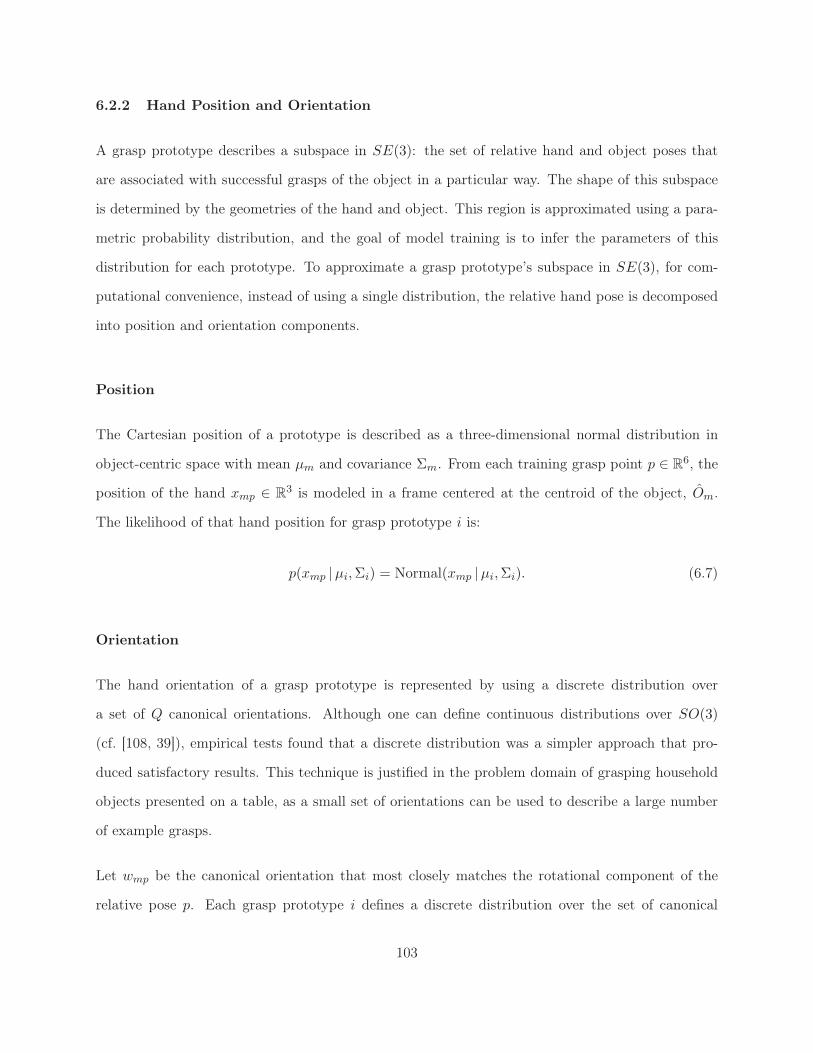
6.2.2 Hand Position and Orientation

A grasp prototype describes a subspace in SE(3): the set of relative hand and object poses that

are associated with successful grasps of the object in a particular way. The shape of this subspace

is determined by the geometries of the hand and object. This region is approximated using a para-

metric probability distribution, and the goal of model training is to infer the parameters of this

distribution for each prototype. To approximate a grasp prototype’s subspace in SE(3), for com-

putational convenience, instead of using a single distribution, the relative hand pose is decomposed

into position and orientation components.

Position

The Cartesian position of a prototype is described as a three-dimensional normal distribution in

object-centric space with mean µm and covariance Σm. From each training grasp point p ∈ R6, the

position of the hand xmp ∈ R3 is modeled in a frame centered at the centroid of the object, Om.

The likelihood of that hand position for grasp prototype i is:

p(xmp |µi,Σi) = Normal(xmp |µi,Σi). (6.7)

Orientation

The hand orientation of a grasp prototype is represented by using a discrete distribution over

a set of Q canonical orientations. Although one can define continuous distributions over SO(3)

(cf. [108, 39]), empirical tests found that a discrete distribution was a simpler approach that pro-

duced satisfactory results. This technique is justified in the problem domain of grasping household

objects presented on a table, as a small set of orientations can be used to describe a large number

of example grasps.

Let wmp be the canonical orientation that most closely matches the rotational component of the

relative pose p. Each grasp prototype i defines a discrete distribution over the set of canonical

103

orientations:

p(wmp |φi) = φi(wmp), (6.8)

where φi is a Q-vector in the (Q−1)-simplex such that φi(q) is the probability of selecting orientation

q.

By using a multinomial model for grasp orientation, each grasp prototype can represent multiple

orientations. This is useful for dealing with the symmetries that can occur when grasping using

Dexter. For example, Dexter can perform a side grasp on an object with the thumb pointing

towards or away from the robot. If the training data consists of both types of grasps, then the grasp

prototype that encodes that particular side grasp will have nonzero probability of choosing both

types of orientation. Note that for each grasp prototype, the probability table over orientation is

built using the training data, so orientations that are more prevalent in the training set are more

likely in the model.

After learning the model, each visual grasp prototype i has a tuple of parameters Ci = (ψi, ui, µi,Σi, φi)

that describe the component distributions over visual appearance and relative hand/object position

and orientation. A pre-grasp is generated from prototype i by sampling from the distributions in

(6.7) and (6.8) using the parameters (µi,Σi, φi) ∈ Ci, described in Section 6.4.1.

6.3 The Generative Model

The previous section described how a grasp prototype is represented as a collection of three paramet-

ric distributions. The generative model presented in this section describes the statistical relationship

between the parameters for a set of A grasp prototypes and the observed training data.

The graphical model is illustrated in Figure 6.3. The nodes of the graph represent random variables,

with the shaded nodes denoting the observed variables. Unshaded nodes are latent variables that

must be inferred from the data. Rectangles around variables denote replication, where the number

of times is shown in the bottom right corner.

104

Σ

b

z

Nm

M

θ

x w

φA

ψ u µ

Figure 6.3. The graphical model described in Section 6.3. Circles indicate random variables, allunshaded variables are latent, shaded variables are observed. A rectangle around nodes representsreplication, with the number of replications written in the bottom right corner. The edges betweennodes indicates a conditional probability relationship described in the text. There are M objectsand A learned visual grasp prototypes, where object m has Nm observations. θ represents theparameters of a multinomial distribution over the set of visual grasp prototypes. z is an indicatorvariable for one of the A prototypes. The observed variables b, x, and w are the object’s visualappearance feature, and the relative hand/object position and orientation, respectively. The bottomrow shows the latent distribution parameters for each of the A visual grasp prototypes: ψ and u aredefine the inverse-Wishart distribution for the visual feature, µ and Σ are the mean and covarianceof the normal distribution describing the Cartesian position of the relative hand/object pose, andφ is the parameter of the multinomial distribution over hand orientation.

105

This model assigns one visual grasp prototype to each data observation; the values of the proto-

types’ distribution parameters are computed after all observations have been assigned. A Bayesian

approach is used to estimate these parameters because of the ability to quantify uncertainty about

their values by using suitable prior distributions.

The training data set D = (b,x,w) is organized into M sets of object grasp features, where set

m has Nm examples. Datum i of object m is the tuple (bmi, xmi, wmi, ), which consists of a visual

feature covariance matrix, the position, and the orientation of the hand, respectively. The variable

z represents the assignment of a prototype to the observed pre-grasp. The variable θ describes a

multinomial distribution over the shared set of prototypes for an object; in effect, it defines a mixture

model over prototypes and describes the likelihood of an object using a particular prototype. Note

that by using a multinomial distribution over the prototypes, independent samples from the model

for the same object can result in a different prototype being selected.

Using this model, the generative process for example pre-grasp i is given below:

θ |α ∼ Dirichlet(α) (6.9)

zi | θ ∼ Multinomial(θ) (6.10)

bi | zi = j ∼ Inv-Wishartuj(ψj) (6.11)

wi | zi = j ∼ Multinomial(φj) (6.12)

xi | zi = j ∼ Normal(µj,Σj). (6.13)

Equation (6.9) samples θ from a symmetric, A-dimensional Dirichlet prior with parameter α. In

(6.10), the prototype assignment zi for this datum is sampled according to θ. The pre-grasp com-

ponents bi, wi, and xi are sampled according to the distributions (6.6), (6.8), and (6.7), described

in Section 6.2, using the parameters of grasp prototype zi.

The multinomial distributions θ and φ are given independent, symmetric Dirichlet priors with pa-

rameters α and β, respectively. The parameters of prior distributions are known as hyperparameters.

106

The second moment covariance prior is inverse-Wishart with scale Ψ and u0 degrees of freedom.

The covariance matrices for grasp position, Σ, also have an inverse-Wishart prior with scale Ξ

and ν degrees of freedom [62]. The grasp position mean is given a uniform prior. For notational

convenience, let Ω correspond to the collection of all hyperparameters used in the model.

6.4 Parameter Estimation in the Model

The inference problem is to compute the posterior distribution of the latent variables given example

pre-grasps, using Bayes’ rule:

p(θ, z,C | D,Ω) =p(D | θ, z,C,Ω) p(θ, z,C |Ω)

p(D |Ω). (6.14)

Computing this in closed-form is intractable, but it can be estimated using Gibbs sampling. Gibbs

sampling is a Markov-chain based technique that is commonly used when it is impossible to sample

from a distribution directly. Instead, one samples from each dimension of the distribution condi-

tioned on the current state of the rest of the dimensions. In this case, the distribution of interest is

the posterior assignment of visual grasp prototypes to data points.

Given the data set D, a Gibbs sampler with auxiliary parameters, as described in Neal [121], is used

to estimate the grasp prototype assignments z. These assignments are then used to provide point

estimates for the other parameters θ and C. In the following, let z−mi denote the set of all grasp

prototype assignments excluding zmi, and let b−mi, x−mi, and w−mi be defined similarly.

Using the conditional independence relationships in the graph of Figure 6.3, the posterior distribu-

tion over grasp prototype assignments can be written as

p(zmi | z−mi,D) ∝ p(zmi | z−mi, om) p(bmi | z,b−mi) p(xmi | z,x−mi) p(wmi | z,w−mi). (6.15)

107

The likelihoods of the conditional grasp prototype assignments and hand orientation assignments

are multinomials, and have been derived from standard Dirichlet integrals:

p(zmi = j|z−mi, om = l) =nO

jl + α∑

j′ nOjl′ +Aα

(6.16)

p(wmi = k|zmi = j, z−mi,w−mi) =nW

kj + β∑

j′ nWkj′ +Qβ

, (6.17)

where nOjl is the number of times grasp prototype j has been assigned to object l, and A is the number

of grasp prototypes shared among all objects. Likewise, nWkj is the number of times orientation

feature k has been assigned to feature j, and Q is the number of canonical grasp orientations.

Since the assignment of grasp prototypes to observations is a statistical process, if A is large there

may be grasp prototypes that are not assigned to any observations. The expected number of grasp

prototypes used is a function of the number of observations and α.

At each iteration of the sampling algorithm, given the current assignment of data points to grasp

prototypes, the posterior distribution over the position of the grasp, xmi, is a multivariate Student-

t distribution with (nAj + ν − 2) degrees of freedom, where nA

j is the total number of features

assigned to grasp prototype j. This can be approximated with the following moment-matched

normal distribution [62]:

p(xmi | zmi = j, z−mi,x−mi) ≈ N (xmi | µj , Σj), (6.18)

where

µj =1

nAj

M∑

m=1

∑

k|zmk=j

xmk (6.19)

Σj = δj

Ξ +M∑

m=1

∑

k|zmk=j

(xmk − µj)(xmk − µj)T

(6.20)

δj =nA

j + 1

nAj (nA

j + ν − 4). (6.21)

108

The conditional distribution for a visual feature covariance is given as

p(bmi | zmi = j, z−mi,b−mi) = Inv-Wishartuj(ψj) (6.22)

with

uj = u0 + nAj (6.23)

ψj =1

nAj

Ψ0 +M∑

m=1

∑

k|zmk=j

bmk

. (6.24)

At each iteration of the Gibbs sampler, equations (6.16) – (6.22) are used to compute (6.15). A

single data point update can be computed in time O(A), and each sample output by the sampler

requires computing this assignment for every training data point. Thus the total time to compute

a sample given a training set with M objects and N grasps per object is O(MNA). The sampler

must be run for a number of “burn-in” iterations before the samples can be considered independent.

In this work, on the order of two hundred “burn-in” iterations were discarded before accepting a

sample.

6.4.1 Generating Pre-Grasps for New Objects

The purpose of the model is to generate candidate pre-grasps for a novel object given visual fea-

tures. Let Θ(s) correspond to model parameters sampled from the posterior distribution after Gibbs

iteration s. The generative process for new pre-grasps given visual feature bt is:

zt | bt, Θ(s) ∼ p(z | bt, Θ

(s)) (6.25)

wt | zt = j, Θ(s) ∼ Multinomial(φ(s)j ) (6.26)

xt | zt = j, Θ(s) ∼ Normal(µ(s)j , Σ

(s)j ). (6.27)

109

With a set of samples from the posterior distribution p(z | D), statistics that are independent of the

content of individual grasp prototypes can be computed by integrating over the full set of samples.

For any single sample Θ(s), θ and C can be estimated using the grasp prototype assignments in z(s)

as described in Section 6.4 using (6.16) – (6.22). These correspond to predictive distributions over

new grasp prototypes and hand positions conditioned on D and z. Note that these estimates cannot

be combined across samples, since there is no guaranteed correspondence between grasp prototypes

among the set of samples.

The distribution in (6.25) can be computed as

p(z = i | bt, Θ(s)) ∝ p(bt | z = i, Θ(s))p(z = i | Θ(s)) ≈ Inv-Wishart

u(s)i

(ψ(s)i ), (6.28)

where p(z = i | Θ) is given as uniform.

Following the generative process in (6.25)–(6.27) produces a set of candidate pre-grasps given a

visual feature. In this work, all grasps are performed using a fixed configuration of the fingers in

the hand, such that they form an opposing grasp. The grasp prototype representation could be

amended to include a distribution over finger configuration to take into account different finger

poses.

6.5 Experimental Results

To test the ability of the model to represent the grasp prototypes demonstrated in the training

set and generate new pre-grasps, the model was trained using a set of household objects. Because

there is no notion of orientation of the object in the model, the same object presented in a different

orientation (flat, standing up, etc.) is treated as a separate object. The notation object-N refers

to the presentation of object in a different orientation. There are examples in the literature of how

this assumption can be relaxed by incorporating the notion of rigid body transformations into the

model itself [147]. A set O of 31 object presentations were chosen for training and testing.

110

babo babo−1 blocks

blocks−1 blocks−2 boy

coke_can comet green_can

jelly lawn_box oxyclean

oxyclean−2 purex purex−1

red_coffee tp vase

whisky−2

Figure 6.4. This picture shows the objects in the training set. The red oval corresponds to thecovariance matrix that was used as a visual feature for grasps with the object.

111

babo−2 black_drano blocks−3

jelly−1 lawn_box−1 lawn_box−2

oxyclean−1 pipe polish

purex−2 whisky whisky−1

Figure 6.5. This picture shows the objects as they were presented for generating grasps.The redoval corresponds to the covariance matrix that was computed from the average second moments ofthe segmented blob in the left and right cameras.

For training, Ntrain = 19 objects were chosen randomly from O, and grasps were demonstrated

using teleoperation. This object set is shown in Figure 6.4. Each object was presented to Dexter

in the middle of the workspace, and the right arm was used to perform all grasps, as shown in

Figure 4.3. While the model specifically generated pre-grasps for Dexter’s right arm, by applying a

known affine transformation to the pre-grasp, they can be used by the left arm. The set of canonical

grasp orientations was computed using the training set, and a set of Q = 6 were chosen. Note that

in these experiments, symmetric grasps were not used, that is, the demonstrator did not perform a

grasp at the same location using a different hand orientation.

112

Figure 6.6. This shows different pre-grasps generated by the model in Section 6.5. The top threepre-grasps were generated by the same grasp prototype, while the bottom two pre-grasps came fromtwo different grasp prototypes.

For learning the parameters of the model, A = 10 shared grasp prototypes were used. The Gibbs

sampler ran for 200 iterations of burn-in, after which the next sample was stored. Using the single

sample, Ntest = 12 objects were presented, shown in Figure 6.5, and the model generated 6 candidate

pre-grasps for each object. The robot achieved each pre-grasp configuration and then attempted to

grasp the object. To perform the grasp, the robot simply flexed its fingers until a sufficient force

had been applied to the object. In these experiments a grasp was judged successful if the robot was

still holding onto the object after moving the hand 10 cm vertically; a sufficient distance to lift the

object off the table. As an example of the types of grasps generated by the model, Figure 6.6 shows

a sequence of five grasps generated for the blocks-3 object.

6.5.1 The Naive Model

A naive model that also generated pre-grasps using visual features was used to analyze the perfor-

mance of the appearance-based model. The naive model performed visual processing to estimate

113

0

1

2

3

4

5

6

Num

ber

of s

ucce

ssfu

l gra

sps

babo

−2

black

_dra

no

block

s−3

jelly−

1

lawn_

box−

1

lawn_

box−

2

oxyc

lean−

1pip

e

polis

h

pure

x−2

whisky

whisky

−1

Comparison of grasp success

Figure 6.7. This graph shows the result of using the trained grasp model on a set of test objects.Each bar measures the number of successful grasps for the labeled object. The blue bars are for thenaive model, and the red for the visual grasp prototype model.

the width and height of the object, and then generated a pre-grasp by selecting points on a spherical

hemisphere centered at the object’s centroid. The radius of the hemisphere was equal to half the

length of the longest dimension of the object. The orientation of the hand was chosen such that

the palm was normal to a ray connecting it to the object’s centroid, and a uniform random rotation

about this ray was chosen. The three fingers of the hand were spread equidistant from each other.

The robot then attempted to grasp the object starting from six different locations, and grasp success

was judged as before.

The results of performing these grasps are shown in Figure 6.7, where blue and red bars correspond

to the naive and visual grasp prototype model, respectively. Overall, the naive model was successful

in 43 out of 72 total grasp attempts. In comparison, using the grasp prototype model, 53 out of

72 attempts were successful; a statistically significant improvement (p < 0.01).

In most cases, the grasp prototype model outperformed the naive approach, including the babo-2

object, which the naive model was unable to grasp. However, the grasp prototype model did have

difficulty with the jelly-1 and whisky-1 objects. In both cases, although the generated pre-grasps

114

were located above the object with a suitable orientation, they were too high for a successful grasp.

This is a result of the fact that the model is in effect summarizing the pre-grasps provided in

the demonstration. For novel objects, the model finds the grasp prototype with the most similar

appearance, but the hand positions suggested by that grasp prototype may not adequately fit the

actual geometries of the object. To improve performance, one could incorporate a grasp controller

to perform the grasp once the pre-grasp was achieved [28]. A more detailed visual appearance

model would also help mitigate such failures, by reducing the chance of visually similar features not

corresponding to similar, successful grasp prototypes.

Since it is based on sampling from a statistical model, the candidate pre-grasps generated by a grasp

prototype may vary in quality, and in these experiments, each candidate pre-grasp was attempted

regardless of its quality. However, as the amount of training data increases, the expected variance of

the grasp prototype distributions will decrease, potentially improving performance. In a real-world

scenario the model could be used interactively, with the teleoperator providing additional training

data to improve the quality of the robot’s hypotheses.

Additionally, the proposed method could be improved by performing a secondary analysis of the

candidate pre-grasps. For example, incorporating additional information about the object geometry

into candidate selection to choose the closest, non-colliding pre-grasp.

The success rate of the model is also affected by the number of shared grasp prototypes. In the

current implementation the number A is estimated based on the number of objects presented,

although one does not know a priori the number of shared grasp prototypes represented in the

training data. If A is too small, the covariances for the position distribution of the grasp prototypes

will be large, so it may require sampling a number of pre-grasps before finding one that is close

enough for a successful grasp. One approach is to use a nonparametric Bayesian method that can

estimate the number of grasp prototypes from the data itself [149].

Table 6.1 illustrates how visual grasp prototypes are shared among different objects, using a single

sample of the posterior to show the composition of each grasp prototype. Each column corresponds

115

Visual Grasp Prototype

1 2 3 4 5 6 7 8 9 10

babo x xbabo-1 xblocks x xblocks-1 x xblocks-2 xboy xcoke_can x xcomet x xgreen_can x xjelly x xlawn_box xoxyclean x xoxyclean-2 xpurex x xpurex-1 xred_coffee x x xtp x xvase xwhisky-2 x

Table 6.1. Each x denotes a grasp on the object in the row that was used by the grasp prototypedenoted in the column. The number of x’s in row i is the number of grasp prototypes used by objecti. The number of x’s in column j is the number of objects that use that grasp prototype j.

to a grasp prototype, and each row denotes the training set of objects. An x indicates that some

training grasp from this object was used to determine the parameters of the grasp prototype in that

column. Columns with multiple x’s indicate a grasp prototype that used training examples from

multiple objects. In this sample, 7 out of 10 grasp prototypes incorporate training examples from

multiple objects. Once the sampler has been run for enough iterations, one can expect subsequent

samples Θ(s) to contain very similar assignments. Different runs of the sampler produce similar

groupings of observations, although the actual assignments to particular grasp prototypes will differ

(e.g., the assignment found in grasp prototype 1 in this sample may be the assignment of grasp

prototype 5 in another sample).

116

6.6 Discussion

This chapter presents a hierarchical, statistical model for representing grasp prototypes among

a collection of objects, using a form of statistical topic model. The model provides a way of

summarizing the data provided by a teleoperator in a way that can be applied to new objects. The

model was shown to proprose candidate pre-grasps that had a statistically significant improvement

over pre-grasps suggested by a baseline model.

For future work, different visual features could be used to learn grasp prototypes specific to smaller

scale features of objects. For example, a set of canonical “visual words” that common visual features

of the geometric structure of an object that is relevant to grasping and common across a range of

objects [148, 144]. As mentioned above, the model can also be improved by incorporating rigid-body

transformations into the representation of objects. Ideally, a model of grasp prototypes is learned

for a canonical orientation of an object, and pre-grasps from that prototype are transformed to

match the orientation of the object as it is presented. Additionally, the model can be combined

with higher-level logic that selects pre-grasp candidates based on task constraints.

More Complex Objects

Using the visual feature model in this chapter, a single object can be represented with multiple

second moment covariances: the model associates a grasp prototype with each covariance, and

they must then be transformed into the appropriate frame. Since the model has no notion of the

geometry of the object beyond centroid and second moment, secondary processing must be used to

filter low-quality pre-grasps. As an example, consider the mallet segmented into two blobs, shown

in Figure 6.1. Using the model learned in the previous section, pre-grasps for each of the two blobs

were generated and manually filtered to remove those that collided with the mallet. For example,

the model generated pre-grasps for side grasps of the handle that would collide with the head of the

mallet. Figure 6.2 shows some feasible candidate pre-grasps suggested by the model.

117

CHAPTER 7

CONCLUSIONS AND FUTURE WORK

In this dissertation, I have presented an architecture for humanoid robot programming by demon-

stration based on sensorimotor schemas. This architecture has been built using the control basis

approach to control as its foundation. In the control basis, behavior is composed by associating

artificial potential functions with sensor and effector resources. The control basis endows the robot

with a basic level of sensorimotor behavior.

Sensorimotor schemas abstract a sequence of controller activations into procedural and declarative

components, and provide the robot with a teleological, control-based perspective for observing and

interpreting a demonstrator’s actions. In Chapter 4, I presented a model that uses the robot’s

control schemas to generate a declarative representation of the demonstration. In Chapter 5, I

introduced a statistical model for learning procedural policies from observation, and provided a

number of experiments illustrating the potential of this approach.

I have focused on object manipulation tasks that fall under the general category of pick and place.

These tasks require the robot to perform a variety of grasps, and in Chapter 6, I described an

approach to pre-grasp generation based on statistical topic models. This model generalizes grasp

prototypes across multiple objects, and allows the robot to predict successful pre-grasps for novel

objects. In this chapter, I recapitulate the main contributions in this dissertation, and discuss areas

of future research.

118

7.1 Contributions

This thesis developed a computational model for robot programming by demonstration based on

the assumption of a robot with a built-in set of sensorimotor behaviors known as schemas. I have

decomposed the PbD problem into declarative and procedural components, and applied different

statistical techniques to learn model parameters from demonstration. Furthermore, I have focused

on the task domain of object manipulation with humanoid robots, and I have proposed a novel

statistical model for pre-grasp generation using visual features.

This dissertation has made contributions to the state of the art in robot programming by demon-

stration in the following areas:

1. Declarative Schema Inference: In Chapter 4, I presented an architecture for declarative

behavior inference from demonstration. In contrast to prior work, the robot interprets the

demonstration by matching sensory observations to expected controller convergence behavior

from its own set of sensorimotor schemas using dynamic statistical inference. This approach

relies on the teleological aspect of closed-loop controllers: the parts of the demonstration asso-

ciated with convergence events create a sequence of observations. The schema most consistent

with the observations is inferred by evaluating a Hidden Markov Model.

A pick and place experiment was peformed to demonstrate the efficacy of the approach, and

illustrated the ability to apply knowledge observed in training to novel scenarios through the

use of schemas. During this experiment, the robot observed a demonstrator perform a sorting

task. The robot was able to identify its pick and place schema as the behavior most consistent

with the demonstration. Using this schema, the robot was able to execute the correct sorting

task. In addition, the robot used the behavioral knowledge built-in to the schema in order to

execute contingencies in the pick and place schema that were never shown by the demonstrator.

For example, although the demonstration was performed using Dexter’s right arm, the robot

executed the task using both arms, as well as transferring an object between arms, by using

the declarative knowledge in the pick and place schema.

119

2. Sensorimotor Schema Proceduralization: Sensorimotor schemas are abstract representa-

tions of teleological behavior; the transitions between component controllers provide structure

for inferring the proper proceduralization of the schema. In Chapter 5, I described a Bayesian

approach to schema proceduralization that integrated prior and demonstrated knowledge. Af-

ter the robot has observed the demonstration, the procedural model is used to apply the

knowledge learned from demonstration to new environments and task instances. The proce-

duralization described in this chapter allows the robot to observe a a discrimination task, such

as sorting, and apply the classification criteria to new environmental contexts. The chapter

also outlines a general framework for developing procedural models given any sensorimotor

schema.

The approach was demonstrated experimentally using a number of sorting tasks that included

classification of both discrete and continuous feature spaces. The Bayesian approach allowed

the robot to maximize the use of prior knowledge and reduce the number of demonstrations

required to successfully learn a classification task.

Furthermore, the generative approach provides a novel way for the robot to communicate how

much it has learned from demonstration to the instructor. By sampling synthetic procedu-

ralizations from the posterior distribution, the instructor is able to visualize and evaluate the

extent to which the robot has learned the correct policy, and refine any further demonstra-

tion in order to maximize the amount of knowledge transfer. This allows the demonstration

process to be performed incrementally, with the goal of minimizing the amount of instruction

needed to teach a task.

3. Approach to Pre-Grasp Generation: In Chapter 6, I presented a statistical model that

learned a set of grasp prototypes using visual features that can be used to generate pre-

grasps for objects. The model used a Bayesian approach that integrated prior knowledge and

demonstration data. When presented with a novel object, the visual features of the object are

associated with a learned set of grasp prototypes. Given the visual features, the appropriate

grasp prototype is sampled in order to generate candidate pre-graps that lead to successful

120

grasps of the object. The model was able to learn grasp prototypes that were shared across

multiple objects, without being explicitly told which objects should be grouped together.

This model was tested experimentally using a set of household objects: the model parameters

were learned after observing demonstration grasps on the training set of objects. After learn-

ing, objects in the test set were presented to the robot, and the pre-grasps generated by the

model were evaluated. These pre-grasps were compared to pre-grasps generated by a naive

model. The visual grasp prototype model produced candidate pre-grasps that resulted in a

statistically significant improvement in grasp success compared to the naive model.

In contrast to existing work, this model provides a way to represent grasp prototypes that are

shared between objects and identifiable by visual features. The model provides a novel way

of learning and representing common grap prototypes across a collection of objects.

7.2 Looking Forward

Humanoid robots are complex machines with vast potential for improving human society. In order

to achieve this, it is essential that roboticists develop powerful, natural programming methods to

enable a basic competency in robot programming for everyone. Research in PbD, including the

work presented in this dissertation, represent the beginnings of this exploration, with much more

remaining to be developed. The work I have presented here poses additional questions and further

avenues of research.

While the work presented in this dissertation has been experimentally validated on Dexter using a

pick and place task domain, it is a general architecture that may be applied to others robots and

tasks. I have focused on pick and place because of its wide adaptability to many different uses for

object manipulation. I have used teleoperation as the method for demonstration, because of its wide

use and the quality of proprioceptive feedback it provides. An immediate avenue of further research

is to apply the models in this work to different experimental platforms that use different methods

of demonstration. Remote observation of demonstration is the most challenging but potentially

121

useful method of demonstration, in that it only requires the robot be able to observe the teacher

performing the task. In order to function in the remote setting, the declarative model of Chapter 4

requires that the robot have a function that can map observations to control inputs for monitors.

Although I assume that the robot has acquired a set of sensorimotor behaviors via design or through

developmental methods, it is natural to learn them from demonstration. The declarative learning

model could be expanded to allow for iterative refinement of existing schemas, by learning new

controller convergence state transitions based on the monitors activated by demonstration. The

next step would be to learn completely new schemas from demonstration.

Another avenue of further research is to expand the declarative inference model of Chapter 4. The

experiments in this work demonstrated the potential of the approach, but furthe experimentation is

required that makes use of multiple potential schemas for behavior matching. The model assumed a

flat task model where each demonstration could be sufficiently explained by a single schema instance;

one option for further research is to relax this assumption to allow the robot to infer sequences of

schema activations from demonstration. Hierarchical extensions to HMMs provide a blueprint for

how the inference model may be enhanced to handle the case of interpreting demonstrations as

reusable sequences of component schemas [23].

The procedural model of Chapter 5 may be extended to other task settings that require alternative

feature models. I have shown how a procedural policy using simple visual features such as color

and shape can be learned from demonstration. This model may be expanded to cover a more

extensive and general set of features. In the vision domain, high-dimensional image descriptors,

such as SIFT [105], may provide a basis for constructing rich, general visual features that can be

applied in many different task contexts. More complex feature models are not confined to vision

however; humanoids with six-axis force/torque sensing fully integrated into hand-like end effectors

will be the standard, and these robots must be able to handle tasks that make use of force-domain

features.

122

The grasp prototype model of Chapter 6 provides many areas of further research. The existing

feature model can be refined to represent more complicated grasp prototypes that allow more precise

and effective grasps. At a more general level, the statistical approach in the grasp prototype model

can be applied to other functional relationships besides pre-grasps. For example, a welding robot

should be able to recognize what types of welds are can be used with different shapes of steel, based

on a collection of demonstration welds. Furthermore, the model can be improved by incorporating

functional requirements into the pre-grasp sampling process. This would allow the model to learn

the relationship between the grasp prototypes and the schemas that use them. When presented with

novel objects, the robot can infer the valid schemas it may execute based on the grasp prototypes

associated with the object.

123

APPENDIX A

INTRODUCTION TO BAYESIAN MODELS

124

A.1 Nonparametric/Semiparametric Bayesian Models

In this section I present a brief review of the Bayesian techniques and semiparametric models used

to perform learning and inference in later chapters. [48]

In this thesis, I take a probabilistic approach to modelling the procedural aspects of a task. By

framing the programming by demonstration paradigm in terms of setting up probability models for

demonstrated tasks, the learning process that occurs post-demonstration is a statistical inference

problem using the data observed during demonstration.

To illustrate the approach, consider a simple demonstrated task: single-armed reaching to a point

in Dexter’s workspace. Each example of the demonstration consists of the expert attempting to

teleoperate Dexter’s right arm to the same point, x⋆, in the workspace and then ending the trial.

Let xi denote the Cartesian position of the Dexter’s hand at the end of trial i. Without loss of

generality, assume that Dexter’s hand orientation is fixed, so xi ∈ R3.

This simple behavior of reaching to a desired location can be modelled declaratively using the reach

controller, cR. The controller takes a Cartesian location r ∈ R6 as a reference. In this example,

since hand orientation is fixed, r ∈ R3.

After demonstration, Dexter has a collection x = x1, . . . , xN ofN observations of the end effector’s

position at the end of the trial. There are a number of sources of noise in this PbD system: the

measurement noise in recording the end effector locations xi, and, more significantly in this example,

the operator noise in the teleoperation signal introduced by putting a human in the loop.

To reproduce the demonstration, the problem for the robot is how to select a reference r given the

examples x? The probabilistic approach assumes that a statistical process with unknown parameters

θ is responsible for generating each xi. For a given task, it is reasonable to further assume that xi

is an independent and identially distributed (iid) random variable. Independent because what is

demonstrated in each trial does not depend on earlier trials, and identically distributed because the

same task is being demonstrated in each trial.

125

A further assumption about x is that the N observations are exchangeable: the joint probability

density p(x1, . . . , xN ) is invariant to permutations of the indices i [14, 62]. In other words, the

ordering of the example trials by the demonstrator does not matter. For the pick and place tasks I

examine in this work, the exchangeability assumption is not a restriction.

A.1.1 Maximum Likelihood Estimates

A reasonable first choice of a model for this example is a multivariate Gaussian (normal) distribution

with mean µ and a d× d covariance matrix Σ:

Normal(xi |µ,Σ) = (2π)−d2 |Σ|−

12 exp

−1

2(xi − µ)T Σ−1(xi − µ)

. (A.1)

That xi has a Gaussian distribution can be denoted xi ∼ Normal(µ,Σ). A Gaussian model, with

θ = (µ,Σ), for the observations x implies a unimodal representation of the target location at µ,

with measurement uncertainty summarized by Σ. The mean µ is a natural choice to use for the

reference r when the robot reproduces this task. The covariance matrix Σ expresses the amount

of variability in the measurement of the example target locations. A demonstrator with access to

Σ would have an idea about how “well” the robot was observing the task, and how much further

demonstration was required. How can the robot estimate θ given the model (A.1) and x?

The likelihood (or sampling distribution) p(x | θ) is the probability density of a set of observations

x under a distribution with parameters θ. The maximum likelihood (ML) estimate finds the value

θML that maximizes the likelihood function

θML = argmaxθ

p(x | θ). (A.2)

Becasue x is iid, the likelihood function can be written as the product of the likelihood of each

individual observation:

p(x | θ) =

N∏

i=1

p(xi | θ). (A.3)

126

For the multivariate Gaussian model, this likelihood function is

p(x |µ,Σ) ∝ |Σ|−n2 exp

−1

2

N∑

i=1

(xi − µ)T Σ−1(xi − µ)

= |Σ|−n2 exp

−1

2tr(Σ−1Sµ)

, (A.4)

where tr(·) is the trace operator, and Sµ is the sum of squares with respect to µ, Sµ =∑N

i=1(xi−µ)2.

Taking the derivative of A.4 and solving for zero, one can find the ML estimate to be the sample

mean and covariance θML = (x, S/N):

x =1

N

N∑

i=1

xi (A.5)

S =

N∑

i=1

(xi − x)2. (A.6)

The maximum likelihood approach provides a point estimate for the mean and covariance of the

model. As N increases, the maximum likelihood estimate θML supplies virtually all the information

about θ available from the data. However, asypmtotic guarantees are not as useful in programming

by demonstration, where the goal is to provide the appropriate training signal in as few examples

as possible.

That maximum likelihood relies solely on the observed data is also one of the drawbacks of using

this approach: it ignores available prior information about θ. Consider the reaching example: if

there is an obstacle in the workspace, this is information that should be included in the inference

of θ.

127

A.1.2 Bayesian Modelling

A Bayesian analysis provides a joint probability model of the data and parameters. Conclusions

about a parameter are made in terms of probability distributions, conditioned on observable data,

and making use of available prior information.

The advantage of this approach is the ability to incorporate prior knowledge into the inference. In

cases where the dataset is small, maximum likelihood estimates are suspectible to bias. However,

consistent incorporation of prior knowledge can improve the accuracy and robustness of the Bayesian

model. The Bayesian framework provides a way for the robot to apply all possible information it

has acquired towards the inference problem presented by the demonstrated task.

In a Bayesian, or generative, model, the observations and the unobserved parameters of the under-

lying statistical process are modelled in a joint probability distribution

p(x, θ). (A.7)

Using the properties of conditional probability, (A.7) can be written as

p(θ,x) = p(x | θ) p(θ), (A.8)

where p(θ) is known as the prior distribution. Often, the prior is expressed as a distribution

p(θ |λ), where the parameters λ are known as hyperparamters. In a hierarchical analysis, the

hyperparameters may also be given a prior distribution p(λ) [14, 62]. However, for the moment,

assume they are fixed with some reasonable value.

Bayes’ theorem is the manipulation of (A.7) to derive the posterior density of θ conditioned on the

observed data:

p(θ |x, λ) =p(x | θ) p(θ |λ)

p(x). (A.9)

128

The denominator of (A.9) is known as the marginal distribution of x, as it can be derived by

marginalizing the joint distribution:

p(x) =

∫

p(x, θ |λ)dθ (A.10)

=

∫

p(x | θ) p(θ |λ)dθ. (A.11)

For the purpose of inferring θ, the data x remains the same, so the marginal density can be considered

a constant factor. For a given set of observations, one often uses the unnormalized posterior density

p(θ |x, λ) ∝ p(x | θ) p(θ |λ). (A.12)

Furthermore, because x is iid, (A.12) can be written as

p(θ |x, λ) ∝ p(θ |λ)N∏

i=1

p(xi | θ). (A.13)

Conjugate prior distributions

Bayes’ theorem provides a way to compute the posterior distribution given a prior and a sampling

distribution, as shown in (A.9). In some cases, by using the appropriate family of distributions to

represent the model, one can compute (A.9) efficiently in closed form. A family of prior distributions

p(θ |λ) is said to be conjugate to the sampling density p(xi | θ) if, for any observation xi and

hyperparameters λ, the posterior density p(θ |xi, λ) remains in that family. This can be summarized

in the following relationship:

p(θ |xi, λ) ∝ p(xi | θ) p(θ |λ)

∝ p(θ | λ), (A.14)

where λ is a modified set of hyperparameters.

129

There exists a class of probability distributions known as the exponential family that are guaranteed

to have the conjugate property. Members of this family include well-known distributions such as

the Bernoulli, Poisson, Gaussian, gamma, and beta distributions. Besides their use as conjugate

priors, members of the exponential family have other desirable properties, such as the existence of

sufficient statistics, that make them widely used in Bayesian analysis [14, 62, 146].

Using Bayesian inference, one infers a posterior distribution p(θ |x) over the model parameters;

in contrast to the point estimate, θML, found using maximum likelihood. Bayes’ rule transfers

information from the prior to the posterior distribution, and there are general properties that relate

these two distributions. The law of iterated expectation can be applied to the posterior distribution

of θ:

E[θ] =

∫ ∫

θ p(θ |x) p(x) dθ dx

=

∫

E[θ |x] p(x) dx

= E[E[θ |x]]. (A.15)

This states that the prior mean of θ is equal to the posterior mean, averaged over the distribution

of the data x. More interestingly, using the standard defintion of variance var(u) = E[u2]− (E[u])2,

one can iterate expectations to derive:

var(θ) = E[var(θ |x)] + var(E[θ |x]). (A.16)

This result implies that on average, the posterior variance is less than the prior variance. The

difference between the two depends on the variance of the posterior mean. To derive this result,

one can work backwards:

130

var(θ) = E[var(θ |x)] + var(E[θ |x])

= E[E[θ2 |x] − (E[θ |x])2] + E[(E[θ |x])2] − (E[E[θ |x]])2

= E[E[θ2 |x]] − E[(E[θ |x])2] + E[(E[θ |x])2] − (E[θ])2

= E[θ2] − (E[θ])2.

As the variation in the var(E[θ |x]) term increases, the uncertainty in the value of θ decreases. The

posterior distribution mean represents a trade-off between the information provided by the prior

and the data. This balance shifts away from the prior as the amount of data increases.

Returning to the reaching task example, given a posterior distribution of θ, there are a number of

ways to select a point estimate θ that can be used for choosing a reference for the reach controller.

Some of the more common choices are the posterior mean:

θ = E[p(θ |x)], (A.17)

and the mode of the posterior, known as the maximum a posteriori estimate:

θMAP = argmaxθ

p(θ |x). (A.18)

For simple parametric models with conjugate priors, (A.17) and (A.18) can be computed in closed

form. However, with models using nonconjugate priors, or more complex hierarchical models, a

closed form for the posterior density is typically intractable. In these cases, one can draw samples

from the posterior using a sampling method to derive an empirical estimate of expectations; this is

discussed in Section A.1.5.

An example using a conjugate prior

The basic model for the simple reaching example is a multivariate Gaussian distribution with d

dimensions over the observed end points xi:

131

xi |µ,Σ ∼ Normal(µ,Σ). (A.19)

The Bayesian approach requires assigning prior distributions to the parameters µ and Σ. To simplify

the example, assume that the covariance matrix Σ is known, thus only a prior for µ is necessary.

Since the likelihood (A.19) is a member of the exponential family, a conjugate prior can be used.

The conjugate prior for µ is the multivariate Gaussian distribution:

µ ∼ Normal(µ0,Λ0), (A.20)

where µ0 and Λ0 are the hyperparameters of the prior.

To derive a posterior density over the unknown parameter µ, combine the likelihood and prior using

Bayes’ theorem,

p(µ |x,Σ) ∝ p(x |µ,Σ) p(µ)

∝ exp

−1

2

[

(µ− µ0)T Λ−1

0 (µ− µ0) +

N∑

i=1

(xi − µ)T Σ−1(xi − µ)

]

, (A.21)

which can be simplified to [62]:

p(µ |x,Σ) ∝ exp

−1

2(µ− µn)T Λ−1

n (µ− µn)

, (A.22)

where

µn = (Λ−10 + nΣ−1)−1(Λ−1

0 µ0 + nΣ−1x)

Λ−1n = Λ−1

0 + nΣ−1. (A.23)

The distribution in (A.22) is also a multivariate Gaussian,

p(µ |x,Σ) = Normal(µ |µn,Λn), (A.24)

illustrating the conjugate property of this combination of likelihood and prior.

132

Sequential data analysis

Another key benefit of the Bayesian approach is the natural way in which it fits into sequential data

analysis problems. The posterior is updated incrementally as each observation arrives, with the

posterior after i− 1 observations acting as the prior for the ith. This can be seen in the following:

p(θ |x1, . . . , xi, λ) ∝ p(x1, . . . , xi | θ) p(θ |λ)

=

i∏

j=1

p(xj | θ) p(θ |λ)

= p(xi | θ) p(θ |x1, . . . , xi−1, λ), (A.25)

where the second line follows from the iid assumption of the data, and the last line results from

rearranging terms and applying Bayes’ theorem.

A.1.3 Mixture Models

Often a single parametric distribution is insufficient for modeling a complex density. A finite mixture

model is a convex combination of a set of kernel functions:

p(x | θ) =

K∑

i=1

πif(x | θi), (A.26)

where f(x | θi) is a kernel (also referred to as a component or cluster) with parameters θi, and

π = π1, . . . , πK,∑πi = 1, is the collection of mixture weights. Each component belongs to

the same family of distributions. Mixtures using Gaussian kernels are known as Gaussian mixture

models with parameters θi = (µi,Σi) [62, 137, 90].

Mixture models can also be described generatively: the mixture weights π form a multinomial

distribution over a set of latent indicator variables z ∈ 1, . . . ,K. The data generating process for

a single observation can be summarized as follows:

133

zi ∼ Multinomial(π)

xi ∼ f(θzi). (A.27)

The value of indicator zi = j determines the parameter θj used to generate the observation. The

generative approach to mixture modeling is known as model-based clustering [17].

An alternative form of the mixture model is to define it in terms of distributions. Let G define a

measure on the parameter space of the component kernels:

G =K∑

k=1

πkδθk(A.28)

where δθkis a Dirac distribution at θk. Then the generative process for obtaining a sample from

such a mixture distribution is:

θi ∼ G

xi ∼ f(θi) (A.29)

For a given value of K, techniques such as expectation maximization (EM) can be used to infer the

parameters of the components. In practice, selecting the correct number of components is a difficult

problem that has been addressed by a number of model selection techniques [15, 111].

Bayesian mixture models

Using EM, one can infer point estimates for the parameters of the mixture. However, in the Bayesian

approach, one infers a distribution over all the parameters in the model. Additionally, priors are

given to the parameters (θ,π) in the mixture distribution [50]. The prior on θ is chosen based on

134

the form of the kernel functions. A conjugate prior can be placed on the mixture weights π by using

a Dirichlet prior with parameters αi:

π ∼ Dirichlet(α1, . . . , αK). (A.30)

Each draw from a Dirichlet distribution is a probability mass function over K elements. If the

concentration parameters are equal, αi = αK , then this is a symmetric Dirichlet distribution. The

symmetry of this mixing prior is in accordance with the exchangeability assumption of the underlying

data: one can relabel the components and the model would remain the same.

Reaching example with a mixture model

Imagine that instead of reaching to a single point in each trial, the demonstrator reaches to one

of two different locations in Dexter’s workspace, depending on the presence or absence of some

stimulus. The simple reaching model can be expanded by using a Gaussian mixture model M with

K = 2 components to represent the data x.

The generative form of this model can be represented as a graph, as shown in Figure A.1. The nodes

in the graph represent variables in the model, while the edges encode the conditional probability

relationships between the variables [91]. The latent paramters are the unfilled nodes, while shading

denotes an observed variable, in this case each reach target xi. Hyperparameters are represented

using rounded boxes. Replication of nodes is denoted by the “plate”, where the subscript indicates

cardinality.

The likelihood of the model M given observations x is computed as:

p(M|x, λ) ∝ p(x |M) p(M|λ) (A.31)

= p(x |θ,π) p(θ,π |λ)

=

K∏

i=1

p(xi | zi, θi)p(zi |π) p(θi |µ0,Σ0) p(π |α). (A.32)

135

θK

zN· · ·

π

α

z1

x1 x2

z2

· · ·θ1

λ

xN N

π

α

θj

zi

xi

λ

K

Figure A.1. The model on the left shows the Gaussian mixture model M in expanded form. Thegraph on the right uses the shorthand notation of “plates” to denote replication across variables.The α and λ variables are hyperparameters, denoted using rounded-edge boxes.

Equation (A.31) is an application of Bayes’ theorem, and the unnormalized likelihood (A.32) follows

from the structure of the graph.

It is typically intractable to compute (A.31) in closed-form. The Monte Carlo methods discussed in

Section A.1.5 can be used to efficiently draw samples from the distribution. Given enough samples,

one can compute approximations to (A.31) with arbitrary accuracy.

A.1.4 Dirichlet Process

The Dirichlet process provides a way to specify a distribution over probability measures; thus it is

commonly used in Bayesian nonparametric statistics as a prior over distributions [143, 18, 52, 116,

92, 68].

Consider a set of exchangeable observations, and let Θ represent a latent parameter space. A

Dirichlet process is defined as follows. Let G0 be a probability distribution on Θ, known as the base

measure, and α a positive scalar, known as the concentration. A Dirichlet process is the distribution

of a random probability measure G over Θ, written G ∼ DP(αG0), such that for any finite partition

136

(A1, . . . , AK) of Θ where

∪Kk=1Ak = Θ

Al ∨Ak 6 = ∅, l 6= k

the random vector (G(A1), . . . , G(AK)) is distributed as a Dirichlet distribution:

(G(A1), . . . , G(AK)) ∼ Dirichlet(αG0(A1), . . . , αG(AK)). (A.33)

Note that the parameters of the Dirichlet distribution in (A.33) are in proportion to the probability

of each set Ai in the base measure. The distribution G is a continuous distribution with non-zero

probability G(Ai) over the set Ai.

Stick-breaking representation

An alternative representation of the Dirichlet process is known as the stick-breaking approach [143].

Let βk ∼ Beta(1, α0), k = 1, 2, . . . be a sequence of Beta random variables. Using this sequence,

define an infinite set of mixing proportions according to:

π1 = β1

πk = βk

ℓ−1∏

ℓ=1

(1 − βℓ), k = 2, 3, . . . (A.34)

The process for computing the set of βk can be seen as taking a unit-length “stick” of probability

mass and breaking it at each πi. It is clear that∑∞

i=1 πi = 1. Now define the random measure

G =∑∞

k=1 πkδθk. It can be shown that G is also a draw from a Dirichlet process [143].

Dirichlet process mixture model

In the case of Bayesian mixture models, one is attempting to infer a distribution over the latent

parameter space, Θ. In the generative view of the model, each data point xi is a sample from a

137

component with parameters θi ∈ Θ. The Dirichlet process provides a way to specify a prior over

the space of distributions. The Dirichlet process mixture model is specified follows:

G ∼ DP(αG0) (A.35)

θi ∼ G, i ∈ 1, . . . , n (A.36)

xi | θi ∼ f(xi | θi), i ∈ 1, . . . , n (A.37)

Since the distribution G is in effect a discrete distribution, in (A.36) it is possible to sample the

same θ for multiple data points. The location and number of distinct θi in the model are a function

of the base measure G0 and concentration α of the Dirichlet process.

A.1.5 Inference using Monte Carlo Methods

The result of many Bayesian analyses is a posterior distribution that one wishes to draw conclusions

from, often in the form of expectations. In many cases these distributions are very complex and

intractable in closed form. Markov chain Monte Carlo (MCMC) methods provide a way to find

approximate solutions to these problems given sufficient compuational power [107, 3, 114].

Let p(x), x ∈ RN represent such an intractable density. Given a set of L samples x(ℓ)Lℓ=1 from

p(x), one can compute the estimator F as

F =1

L

∑

ℓ

f(x(ℓ)). (A.38)

The MCMC algorithm produces samples of p(x) by exploring the underlying state space using a

Markov chain technique. If x(0) is an initial state, each subsequent state x(i) is generated according

to the Markov process

x(i) ∼ q(x |x(i−1)). (A.39)

138

A transition distribution q is said to be irreducible if from any state there is nonzero probability of

visting all other states. An aperiodic chain is one free of cycles. MCMC samplers are irreducible

and aperiodic Markov chains that produce the target p(x) as the invariant distribution, i.e., after a

number of iterations L, x(L) is a sample from p(x) [3].

Gibbs sampling

The Gibbs sampler [61] is a specialized form of MCMC sampler that works well with state spaces

where the conditional density is easily sampled from [113, 78, 3, 107].

Let x = (x1, . . . , xN ) be the sample space decomposed into a vector of N components. At each

iteration i, the idea behind the Gibbs sampler is to sample each dimension x(i)j conditioned on the

values of the other N − 1 dimensions. For a single iteration, x(i+1) is sampled as:

x(i+1)1 ∼ p(x1 |x

(i)2 , . . . , x

(i)N ) (A.40)

x(i+1)2 ∼ p(x2 |x

(i+1)1 , x

(i)3 , . . . , x

(i)N ) (A.41)

...

x(i+1)N ∼ p(xN |x

(i+1)1 , . . . , x

(i+1)N−1 ). (A.42)

For many Bayesian models, the conditional densities are tractable, particularly if conjugate priors

are used, and one can often generate samples using closed forms. I use Gibbs sampling extensively

in the later chapters of this thesis to derive approximations to posterior distributions of interest.

139

APPENDIX B

OBJECTS USED IN EXPERIMENTS

140

B.1 Objects Used in Experiments

This appendix details the objects used in the experiments of Chapter 5. Figures B.1–B.4 show each

object presentation associated with the color categories used in Section 5.1.2. The color categories

were assigned by hand. The inset is a normalized histogram over the 64 value HSV color space,

computed over all the pixels in the object segment.

Figures B.5–B.7 show each object presentation, grouped according to its hand-labeled size category.

141

jif

1 640

1

jif1−1

1 640

1

jif1−2

1 640

1

jif2

1 640

1

oxyclean1

1 640

1

oxyclean1−2

1 640

1

oxyclean2

1 640

1

pink_drano1

1 640

1

pink_drano1−1

1 640

1

pink_drano1−2

1 640

1

pink_drano2

1 640

1

pink_drano2−1

1 640

1

pink_drano2−2

1 640

1

red_coffee1

1 640

1

red_coffee1−1

1 640

1

red_coffee1−2

1 640

1

red_football1

1 640

1

red_football1−1

1 640

1

red_pipe1

1 640

1

red_pipe1−1

1 640

1

red_pipe2

1 640

1

taz1

1 640

1

taz2

1 640

1

taz3

1 640

1

Figure B.1. There are 24 object presentations classified as Red.

142

blue_ball1

1 640

1

blue_pipe1

1 640

1

blue_pipe1−1

1 640

1

blue_pipe1−2

1 640

1

blue_pipe1−2

1 640

1

blue_pipe1−3

1 640

1

jelly1

1 640

1

jelly1−1

1 640

1

jelly2

1 640

1

purex1

1 640

1

purex1−1

1 640

1

purex1−2

1 640

1

purex1−3

1 640

1

purex2

1 640

1

purex2−2

1 640

1

purex2−3

1 640

1

soap1

1 640

1

soap1−1

1 640

1

Figure B.2. There are 18 object presentations classified as Blue.

143

babo1

1 640

1

babo2

1 640

1

butter_box1

1 640

1

butter_box1−1

1 640

1

butter_box1−2

1 640

1

butter_box1−3

1 640

1

butter_box1−4

1 640

1

butter_box2

1 640

1

butter_box2−1

1 640

1

butter_box2−2

1 640

1

butter_box2−3

1 640

1

gs_box1

1 640

1

gs_box1−1

1 640

1

gs_box1−2

1 640

1

shampoo1

1 640

1

shampoo1−1

1 640

1

shampoo2

1 640

1

Figure B.3. There are 17 object presentations classified as White.

144

bk_drano1

1 640

1

bk_drano1−1

1 640

1

bk_drano1−2

1 640

1

bk_drano1−3

1 640

1

bk_drano2

1 640

1

bk_pipe1

1 640

1

bk_pipe1−1

1 640

1

bk_pipe1−2

1 640

1

bk_pipe1−3

1 640

1

black_football1

1 640

1

gray_drano1

1 640

1

gray_drano1−1

1 640

1

Figure B.4. There are 12 object presentations classified as Black.

145

bk_drano1−3 black_football1 blue_ball1 butter_box1−1 butter_box2−1

comet1 comet2 gray_drano1−2 gray_drano1−3 green_box1

green_box1−1 grn_drano1−2 jelly1 jelly1−1 jelly2

jif orng_ball1 orng_football1 orng_football1−1 oxyclean1

oxyclean1−1 oxyclean1−2 oxyclean2 pooh_ball1 purex1−1

red_coffee1 red_football1 red_football1−1 red_pipe1 red_pipe1−1

red_pipe2 shampoo1 shampoo1−1 shampoo2 soap1

soap1−1 twine1 twine2

Figure B.5. There are 38 object presentations classified as Small.

146

babo1 babo2 bk_drano1 bk_drano1−1 bk_drano1−2

bk_drano2 bk_pipe1 bk_pipe1−1 bk_pipe1−2 bk_pipe1−3

blue_pipe1−1 butter_box1−3 butter_box2−2 butter_box2−3 gray_drano1

gray_drano1−1 gray_drano2 green_box1−2 green_box1−3 grn_drano1

grn_drano1−1 grn_drano2 grn_drano2−1 gs_box1−1 jif1−1

jif1−2 jif2 lawn_box1−1 polish1 polish2

purex1 purex1−2 purex1−3 purex2 purex2−2

purex2−3 red_coffee1−1 red_coffee1−2 whisky1−2

Figure B.6. There are 39 pbject presentations classified as Medium.

147

blue_pipe1 blue_pipe1−2 blue_pipe1−3 butter_box1

butter_box1−2 butter_box1−4 butter_box2 gray_drano2−1

gs_box1 gs_box1−2 lawn_box1 lawn_box1−2

lawn_box1−3 lawn_box2 pink_drano1 pink_drano1−1

pink_drano1−2 pink_drano2 pink_drano2−1 pink_drano2−2

taz1 taz2 taz3 whisky1

whisky1−1 whisky1−3 whisky1−4 whisky1−5

whisky2 whisky2−1 whisky2−3

Figure B.7. There are 31 object presentations classified as Large.

148

BIBLIOGRAPHY

[1] Aleotti, Jacopo, and Caselli, Stefano. Trajectory clustering and stochastic approximationfor robot programming by demonstration. In Proceedings of the IEEE/RSJ InternationalConference on Intelligent Robots and Systems (IROS) (August 2005), pp. 1029–1034.

[2] Amit, R., and Matarić, Maja. Learning movement sequences from demonstration. In Proceed-ings of the International Conference on Development and Learning (ICDL) (2002), pp. 203–208.

[3] Andrieu, Christophe, Freitas, Nando De, Doucet, Arnaud, and Jordan, Michael I. An intro-duction to MCMC for machine learning. Machine Learning 50 (2003), 5–43.

[4] Angros, Jr., Richard Harrington. Learning what to Instruct: Acquiring Knowledge fromDemonstrations and Focussed Experimentation. PhD thesis, University of Southern California,Los Angeles, CA, May 2000.

[5] Arbib, Michael A., Billard, Aude, Iacoboni, Marco, and Oztop, Erhan. Synthetic brain imag-ing: grasping, mirror neurons and imitation. Neural Networks 13 (2000), 975–997.

[6] Asada, Haruhiko, and Izumi, Haruo. Direct teaching and automatic program generation forthe hybrid control of robot manipulators. In Proceedings of the IEEE International Conferenceon Robotics and Automation (ICRA) (1987), IEEE, pp. 1401–1406.

[7] Asada, Minoru, Yoshikawa, Yuichiro, and Hosoda, Koh. Learning by observation withoutthree-dimensional reconstruction. In Proceedings of Intelligent Autonomous Systems (IAS-6)(2000), pp. 555–560.

[8] Astington, Janet Wilde. The paradox of intention: Assessing children’s metarepresentationalunderstanding. In Intentions and Intentionality: Foundations of Social Cognition, Bertram F.Malle, Louis J. Moses, and Dare A. Baldwin, Eds. The MIT Press, Cambridge, MA, 2001,ch. 4, pp. 85–103.

[9] Atkeson, Christopher G., and Schaal, Stefan. Learning tasks from a single demonstration.In Proceedings of the International Conference on Robotics and Automation (ICRA) (Albu-querque, NM, April 1997), vol. 3, IEEE, pp. 1706–1712.

[10] Atkeson, Christopher G., and Schaal, Stefan. Robot learning from demonstration. In Proceed-ings of the Fourteenth International Conference on Machine Learning (ICML) (1997), vol. 14,pp. 12–20.

149

[11] Baum, L.E. An inequality and associated maximization technique in statistical estimation forprobabilistic functions of markov processes. Inequalities 3, 1 (1972), 1–8.

[12] Baum, LE, and Egon, JA. An inequality for rational functions with applications to somesta-tistical estimation problems. Bull. Amer. Metereol. Soc 73 (1968), 211–227.

[13] Bentivegna, Darrin C., Ude, Ales, Atkeson, Christopher G., and Cheng, Gordon. Humanoidrobot learning and game playing using PC-based vision. In Proceedings of the IEEE/RSJInternational Conference on Intelligent Robots and Systems (IROS) (2002), vol. 3, pp. 2449–2454.

[14] Bernardo, José M., and Smith, Adrian F. M. Bayesian Theory. John Wiley & Sons, Ltd.,2000.

[15] Biernacki, Christophe, Celeux, Gilles, and Govaert, Gérard. Assessing a mixture model forclustering with the integrated completed likelihood. IEEE Transactions on Pattern Analysisand Machine Intelligence 22, 7 (July 2000), 719–725.

[16] Billard, Aude, and Matarić, Maja J. Learning human arm movements by imitation: evaluationof a biologically inspired connectionist architecture. Robotics and Autonomous Systems, 941(2001), 1–16.

[17] Bishop, Christopher M. Latent variable models. In Learning in Graphical Models, Michael I.Jordan, Ed. The MIT Press, 1998, pp. 371–403.

[18] Blackwell, David, and MacQueen, James B. Ferguson distributions via Poĺya urn schemes.The Annals of Statistics 1, 2 (March 1973), 353–355.

[19] Blei, David M., Ng, Andrew Y., and Jordan, Michael I. Latent Dirichlet allocation. Journalof Machine Learning Research 3 (2003), 993–1022.

[20] Breazeal, Cynthis, and Scassellati, Brian. Robots that imitate humans. Trends in CognitiveSciences 6, 11 (November 2002), 481–487.

[21] Buccino, G., Binkofskli, F., Fink, G. R., Fadiga, L., Fogassi, L., Gallese, V., Seitz, R. J., Zilles,K., Rizzolatti, G., and Freund, H.-J. Action observation activates premotor and parietal areasin a somatotopic manner: an fMRI study. European Journal of Neuroscience 13 (2001), 400–404.

[22] Buccino, Giovanni, Vogt, Stefan, Ritzl, Afra, Fink, Gereon R., Zilles, Karl, Freund, Hans-Joachim, and Rizzolatti, Giacomo. Neural circuits underlying imitation learning of handactions: An event-related fMRI study. Neuron 42 (April 2004), 323–334.

[23] Bui, Hung H., Phung, Dinh Q., and Venkatesh, Svetha. Hierarchical hidden Markov modelswith general state hierarchy. In Proceedings of the National Conference on Artificial Intelli-gence (2004), no. 19, AAAI, pp. 324–329.

[24] Byrne, Richard W., and Russon, Anne E. Learning by imitation: A hierarchical approach.Behavioral and Brain Sciences 21 (1998), 667–721.

150

[25] Canny, J.F. The Complexity of Robot Motion Planning. MIT Press, Cambridge, MA, 1988.

[26] Chen, Jason, and Zelinsky, Alex. Programing by demonstration: Coping with suboptimalteaching actions. The International Journal of Robotics Research 22, 5 (May 2003), 299–319.

[27] Chen, Jason R. Constructing task-level assembly strategies in robot programming by demon-stration. The International Journal of Robotics Research 24, 12 (December 2005), 1073–1085.

[28] Coelho, J. Multifingered Grasping: Haptic Reflexes and Control Context. PhD thesis, Univer-sity of Massachusetts, Amherst, MA, September 2001.

[29] Coelho, J., Araujo, EG, Huber, M, and Grupen, R. Dynamical categories and control policyselection. In Proceedings of the ISIC/CIRA/ISAS’98 Conference (Gaithersburg, MD, 1998),IEEE.

[30] Coelho, J., and Grupen, R. Online grasp synthesis. In Proceedings of the Conference onRobotics and Automation (Minneapolis, MN, April 1996), IEEE.

[31] Coelho, JA, and Grupen, RA. A control basis for learning multifingered grasps. Journal ofRobotic Systems 14, 7 (1997), 545–557.

[32] Connolly, C., and Grupen, R. On the applications of harmonic functions to robotics. Journalof Robotics Systems 10, 7 (1993), 931–946.

[33] Craig, John J. Introduction to Robotics: Mechanics and Control, third ed. Series in Electricaland Computer Engineering: Control Engineering. Addison-Wesley, Reading, MA, 1989.

[34] Creem-Regehr, Sarah H., and Lee, James N. Neural representations of graspable objects: aretools special? Cognitive Brain Research 22 (2005), 457–469.

[35] Csibra, Gergely. Teleological and referential understanding of action in infancy. PhilosophicalTransactions of the Royal Society of London, Series B 358 (2003), 447–458.

[36] Csibra, Gergely, Bíró, Szilvia, Koós, Orsolya, and Gergely, György. One-year-old infants useteleological representations of actions productively. Cognitive Science 27 (2003), 111–133.

[37] Csibra, Gergely, and Gergely, György. The teleological origins of mentalistic action explana-tions: A developmental hypothesis. Developmental Science 1, 2 (1998), 255–259.

[38] Dautenhahn, Kerstin, and Nehaniv, Chrystopher L., Eds. Imitation in Animals and Artifacts.The MIT Press, Cambridge, Massachusetts, 2002.

[39] de Granville, Charles, Southerland, Joshua, and Fagg, Andrew H. Learning grasp affordancesthrough human demonstration. In Proceedings of the International Conference on Develop-ment and Learning (ICDL) (2006).

[40] Dean, Thomas, and Kanazawa, Keiji. A model for reasoning about persistance and causation.Computational Intelligence 5, 3 (1989), 142–150.

[41] Delson, Nathan, and West, Harry. Robot programming by human demonstration: Adaptationand inconsistency in constrained motion. In Proceedings of the IEEE International Conferenceon Robotics and Automation (ICRA) (Minneapolis, Minnesota, April 1996), IEEE, pp. 30–36.

151

[42] Dempster, A. P., Laird, N. M., and Rubin, Donald B. Maximum likelihood from incompletedata via the EM algorithm. Journal of the Royal Statistical Society, Series B (Methodology)39, 1 (1977), 1–38.

[43] Dillmann, Rüdiger. Teaching and learning of robot tasks via observation of human perfor-mance. Robotics and Autonomous Systems 47, 2,3 (June 2004), 109–116.

[44] Dillmann, Rüdiger, Kaiser, M., and Ude, Ales. Acquisition of elementary robot skills fromhuman demonstration. In Proceedings of the International Symposium on Intelligent RoboticSystems (SIRS) (Pisa, Italy, 1995).

[45] Dixon, Kevin R., Dolan, John M., and Khosla, Pradeep K. Predictive robot programming:Theoretical and experimental analysis. The International Journal of Robotics Research 23, 9(September 2004), 955–973.

[46] Drumwright, Evan, Jenkins, Odest Chadwicke, and Matarić, Maja. Exemplar-based primi-tives for humanoid movement classification and control. In Proceedings of the InternationalConference on Robotics and Automation (ICRA) (New Orleans, LA, 2004), IEEE.

[47] Drumwright, Evan, and Matarić, Maja J. Generating and recognizing free-space movementsin humanoid robots. In Proceedings of the IEEE/RSJ International Conference on IntelligentRobots and Systems (IROS) (Las Vegas, NV, 2003), IEEE/RSJ.

[48] Duda, Richard O., Hart, Peter E., and Stork, David G. Pattern Classification, second ed.John Wiley & Sons, Inc., 2001.

[49] Ellis, Rob, and Tucker, Mike. Micro-affordance: The potentiation of components of action byseen objects. British Journal of Psychology 91 (2000), 451–471.

[50] Escobar, Michael D., and West, Mike. Bayesian density estimation and inference using mix-tures. Journal of the American Statistical Association 90, 430 (June 1995), 577–588.

[51] Fagg, Andrew H., and Arbib, Michael A. Modeling parietal-premotor interactions in primatecontrol of grasping. Neural Networks 11 (1998), 1277–1303.

[52] Ferguson, Thomas S. A Bayesian analysis of some nonparametric problems. Annals of Statis-tics 1, 2 (March 1973), 209–230.

[53] Fikes, R.E, and Nilsson, N.J. Strips: A new approach to the application of theorem provingto problem solving. Artificial Intelligence 2, 3,4 (1971).

[54] Flanagan, J. Randall, and Johansson, Roland S. Actions plans used in action observation.Nature 424, 14 (August 2003), 769–771.

[55] Fogassi, Leonardo, Ferrari, Pier Francesco, Gesierich, Benno, Rozzi, Stefano, Chersi, Fabian,and Rizzolatti, Giacomo. Parietal lobe: From action organization to intention understanding.Science 308 (April 2005), 662–667.

[56] Friedrich, H., Münch, S., Dillmann, R., Bocionek, S., and Sassin, M. Robot programming bydemonstration (RPD): Supporting the induction by human interaction. Machine Learning 23(1996), 163–189.

152

[57] Friedrich, Holger, and Dillmann, Rüdiger. Robot programming based on a single demonstra-tion and user intentions. In Proceedings of the European Workshop on Learning Robots atECML (1995).

[58] Frith, Chris D., and Frith, Uta. Interacting minds — a biological basis. Science 286 (November1999), 1692–1695.

[59] Gallese, Vittorio, Keysers, Christian, and Rizzolatti, Giacomo. A unifying view of the basisof social cognition. Trends in Cognitive Science 8, 9 (September 2004), 396–403.

[60] Garland, Andrew, and Lesh, Neal. Learning hierarchical task models by demonstration. Tech.Rep. TR2003-01, Mitsubishi Research Laboratories, January 2003.

[61] Gelfand, Alan E., and Smith, Adrian F. M. Sampling-based approaches to calculating marginaldensities. Journal of the American Statistical Association 85, 410 (June 1990), 398–409.

[62] Gelman, Andrew, Carlin, John B., Stern, Hal S., and Rubin, Donald B. Bayesian DataAnalysis, second ed. Texts in Statistical Science. Chapman & Hall/CRC, 2004.

[63] Gergely, György. What should a robot learn from an infant? Mechanisms of action inter-pretation and observational learning in infancy. In Proceedings of the Third InternationalWorkshop on Epigenetic Robotics (Boston, MA, August 2003), Christopher G. Prince, LucBerthouze, Hideki Kozima, Daniel Bullock, Georgi Stojanov, and Christian Balkenius, Eds.,Lund University Cognitive Studies, pp. 13–24.

[64] Gergely, György, Bekkering, Harold, and Király, Ildikó. Rational imitation in preverbal in-fants. Nature 415 (February 2002), 755.

[65] Gergely, György, and Csibra, Gergely. Teleological reasoning in infancy: The infant’s naivetheory of rational action, a reply to Premack and Premack. Cognition 63 (1997), 227–233.

[66] Gergely, György, and Csibra, Gergely. Teleological reasoning in infancy: the naïve theory ofrational action. Trends in Cognitive Science 7, 7 (July 2003), 287–291.

[67] Gergely, György, Nádasdy, Zoltán, Csibra, Gergely, and Bíró, Szilvia. Taking the intentionalstance at 12 months of age. Cognition 56, 2 (August 1995), 165–193.

[68] Ghahramani, Zoubin. Non-parametric Bayesian methods. Tutorial in Uncertainty in ArtificialIntelligence (UAI), July 2005.

[69] Gibson, James J. The theory of affordances. In Perceiving, Acting, and Knowing, RobertShaw and John Bransford, Eds. Lawrence Erlbaum Associates, Hillsdale, New Jersey, 1977,ch. 3, pp. 67–82.

[70] Griffiths, Thomas L., and Steyvers, Mark. Finding scientific topics. In Proceedings of theNational Academy of Sciences (2004), vol. 101, pp. 5228–5235.

[71] Grudic, Gregory Z., and Lawrence, Peter D. Human-to-robot skill transfer using the SPOREapproximation. In Proceedings of the IEEE International Conference on Robotics and Au-tomation (ICRA) (Minneapolis, Minnesota, April 1996), vol. 4, IEEE, pp. 2962–2967.

153

[72] Grupen, R., and Souccar, K. Manipulability-based spatial isotropy: A kinematic reflex. InWorkshop on Mechatronical Computer Systems for Perception and Action (Halmstad, SWE-DEN, June 1-3 1993).

[73] Guyon, Isabelle, and Elisseeff, André. An introduction to variable and feature selection.Journal of Machine Learning Research 3 (March 2003), 1157–1182.

[74] Hart, Stephen, and Grupen, Rod. Natural task decomposition with intrinsic potential fields.In Proceedings of the International Conference on Intelligent Robotics and Systems (IROS)(San Diego, CA, 2007).

[75] Hart, Stephen, Sen, Shiraj, and Grupen, Rod. Intrinsically motivated hierarchical manipu-lation. In Proceedings of the International Conference on Robotics and Automation (ICRA)(2008).

[76] Hart, Stephen W. The Development of Hierarchical Knowledge in Robot Systems. PhD thesis,University of Massachusetts Amherst, Sep 2009.

[77] Hart, Stephen W., Ou, Shichao, Sweeney, John D., and Grupen, Roderic A. A frameworkfor learning declarative structure. In Workshop on Manipulation for Human Environments,Robotics: Science and Systems (Philadelphia, PA, August 2006).

[78] Hastings, W. K. Monte Carlo sampling methods using Markov chains and their applications.Biometrika 57, 1 (April 1970), 97–109.

[79] Hayes, Gillian, and Demiris, John. A robot controller using learning by imitation. In Pro-ceedings of the International Symposium on Intelligent Robotic Systems (SIRS) (Grenoble,France, July 1994).

[80] Heckerman, David. A tutorial on learning with Bayesian networks. In Jordan [90], pp. 301–354.

[81] Hovland, Geir E., Sikka, Pavan, and McCarragher, Brenan J. Skill acquisition from humandemonstration using a hidden markov model. In Proceedings of the IEEE International Con-ference on Robotics and Automation (ICRA) (Minneapolis, Minnesota, April 1996), IEEE,pp. 2706–2711.

[82] Huber M, Grupen RA. A feedback control structure for on-line learning tasks. Journal ofRobots and Autonomous Systems 22, 3-4 (1997), 303–315.

[83] Iacoboni, Marco, Molnar-Szakacs, Istvan, Gallese, Vittorio, Buccino, Giovanni, Mazziotta,John C., and Rizzolatti, Giacomo. Grasping the intentions of others with one’s own mirrorneuron system. PLoS Biology 3, 3 (March 2005), e79.

[84] Iacoboni, Marco, Woods, Roger P., marcel Brass, Bekkering, Harold, Mazziotta, John C., andRizzolatti, Giacomo. Cortical mechanisms of human imitation. Science 286 (December 1999),2526–2528.

[85] Ijspeert, Auke Jan, Nakanishi, Jun, and Schaal, Stefan. Learning rhythmic movements bydemonstration using nonlinear oscillators. In Proceedings of the IEEE/RSJ InternationalConference on Intelligent Robots and Systems (IROS) (Lausanne, Switzerland, September2002), IEEE/RSJ.

154

[86] Ijspeert, Auke Jan, Nakanishi, Jun, and Schaal, Stefan. Movement imitation with nonlineardynamical systems in humanoid robots. In Proceedings of the IEEE International Conferenceon Robotics and Automation (ICRA) (Washington, D.C., May 2002), IEEE, pp. 1398–1403.

[87] Jenkins, Odest Chadwicke, and Matarić, Maja J. Deriving action and behavior primitives fromhuman motion data. In Proceedings of the IEEE/RSJ International Conference on IntelligentRobots and Systems (IROS) (Lausanne, Switzerland, September 2002), IEEE/RSJ, pp. 2251–2556.

[88] Jenkins, Odest Chadwicke, and Matarić, Maja J. A spatio-temporal extension to isomapnonlinear dimension reduction. In Proceedings of the International Conference on MachineLearning (ICML) (Banff, Canada, 2004), pp. 441–448.

[89] Jones, J.L., and Lozano-Pérez, T. Planning two-fingered grasps for pick-and-place operationson polyhedra. In Proceedings of 1990 Conference on Robotics and Automation (May 1990),IEEE, pp. 683–688.

[90] Jordan, Michael I., Ed. Learning in Graphical Models. Adaptive Computation and MachineLearning. The MIT Press, Cambridge, MA, 1998.

[91] Jordan, Michael I. Graphical models. Statistical Science 19, 1 (2004), 140–155.

[92] Jordan, Michael I. Dirichlet processes, Chinese restaurant processes and all that. Tutorial inNeural Information Processing Systems (NIPS), 2005.

[93] Juang, BH, and Rabiner, LR. Hidden markov models for speech recognition. Technometrics33, 3 (1991), 251–272.

[94] Kaiser, M., and Dillmann, R. Building elementary robot skills from human demonstration. InProceedings of the International Conference on Robotics and Automation (ICRA) (Minneapo-lis, Minnesota, April 1996), IEEE.

[95] Kang, Sing Bing, and Ikeuchi, Katsushi. Toward automatic robot instruction from perception–recognizing a grasp from observation. IEEE Transactions on Robotics and Automation 9, 4(Aug 1993), 432–443.

[96] Kang, Sing Bing, and Ikeuchi, Katsushi. Toward automatic robot instruction from perception–temporal segmentation of tasks from human hand motion. IEEE Transactions on Roboticsand Automation 11, 5 (Oct 1995), 670–681.

[97] Khatib, Oussama. Real-time obstacle avoidance for manipulators and mobile robots. InProceedings of the International Conference on Robotics and Automation (ICRA) (Mar 1985),vol. 2, IEEE, pp. 500–505.

[98] Khatib, Oussama. A unified approach for motion and force control of robot manipulators:The operational space formulation. IEEE Journal of Robotics and Automation RA-3, 1 (Feb1987), 43–53.

[99] Koditschek, D.E., and Rimon, E. Robot navigation functions on manifolds with boundary.Advances in Applied Mathematics 11, 4 (1990), 412–442.

155

[100] Kohler, Evelyne, Keysers, Christian, Umiltá, M. Alessandra, Fogassi, Leonard, Gallese, Vitto-rio, and Rizzolatti, Giacomo. Hearing sounds, understanding actions: Action representationin mirror neurons. Science 297 (August 2002), 846–848.

[101] Kuniyoshi, Yasuo, Inaba, Masayuki, and Inoue, Hirochika. Learning by watching: Extractingresuable task knowledge from visual observation of human performance. IEEE Transactionson Robotics and Automation 10, 6 (December 1994), 799–822.

[102] Kuniyoshi, Yasuo, Inoue, Hirochika, and Inaba, Masayuki. Design and implementation ofa system that generates assembly programs from visual recognition of human action se-quences. In Proceedings of the International Workshop on Intelligent Robots and Systems(IROS) (Ibaraki, Japan, Jul 1990), vol. 2, IEEE, pp. 567–574.

[103] Liapunov, A.M. Stability of Motion. Academic Press, New York, NY, 1966.

[104] Lopes, Manuel Cabido, and Santos-Victor, José. Visual learning by imitation with motorrepresentations. IEEE Transactions on Systems, Man, and Cybernetics, Part B 35, 3 (June2005), 438–449.

[105] Lowe, David G. Distinctive image features from scale-invariant keypoints. InternationalJournal of Computer Vision 60, 2 (2004), 91–110.

[106] Lozano-Pérez, Tomás, Jones, Joseph L., Mazer, Emmanuel, and O’Donnell, Patrick A. Task-level planning of pick-and-place robot motions. Computer 22, 3 (March 1989), 21–29.

[107] MacKay, David J. C. Information Theory, Inference, and Learning Algorithms. CambridgeUniversity Press, 1995.

[108] Mardia, Kanti V., and Jupp, Peter E. Directional Statistics, second ed. John Wiley & Sons,Ltd., 2000.

[109] Matarić, Maja J. Getting humanoids to move and imitate. IEEE Intelligent Systems(July/August 2000), 18–24.

[110] Matarić, Maja J. Sensory-motor primitives as a basis for imitation: Linking perception toaction and biology to robotics. In Dautenhahn and Nehaniv [38], ch. 15, pp. 392–422.

[111] McLachlan, G. J. On bootstrapping the likelihood ratio test statistics for the number ofcomponents in a normal mixture. Applied Statistics 36, 3 (1987), 318–324.

[112] Meltzoff, Andrew N. Infant imitation after a 1-week delay: Long-term memory for novel actsand multiple stimuli. Developmental Psychology 24, 4 (1988), 470–476.

[113] Metropolis, Nicholas, Rosenbluth, Arianna W., Rosenbluth, Marshall N., Teller, Augusta H.,and Teller, Edward. Equation of state calculations by fast computing machines. The Journalof Chemical Physics 21, 6 (June 1953), 1087–1092.

[114] Metropolis, Nicholas, and Ulam, S. The Monte Carlo method. Journal of the AmericanStatistical Association 44, 247 (September 1949), 335–341.

156

[115] Miyata, Natsuki, Oguri, Kenichiro, Ota, Jun, and Arai, Tamio. Human lift-up motion gen-eration based on identification of time-invariant performance index. In Proceedings of theIEEE/RSJ International Conference on Intelligent Robots and Systems (IROS) (Lausanne,Switzerland, September 2002), IEEE/RSJ, pp. 2503–2508.

[116] Muller, Peter, and Quintana, Fernando A. Nonparametric bayesian data analysis. StatisticalScience 19, 1 (2004), 95–110.

[117] Mussa-Ivaldi, F. A., Giszter, S. F., and Bizzi, E. Linear combinations of primitives in ver-tebrate motor control. Proceedings of the National Academy of Science USA 91 (Aug 1994),7534–7538.

[118] Nakamura, Yoshihiko. Advanced Robotics: Redundancy and Optimization. Addison-WesleyLongman Publishing Co., Inc., 1990.

[119] Nakamura, Yoshihiko. Advanced Robotics: Redundancy and Optimization. Addison-WesleyPublishing Company, Inc., 1991.

[120] Nakanishi, Jun, Cory, Rick, Mistry, Michael, Peters, Jan, and Schaal, Stefan. Operationalspace control: A theoretical and empirical comparison. The International Journal of RoboticsResearch 27, 6 (June 2008), 737–757.

[121] Neal, Radford M. Markov chain sampling methods for Dirichlet process mixture models.Journal of Computational and Graphical Statistics 9, 2 (2000), 249–265.

[122] Nehaniv, Chrystopher L., and Dautenhahn, Kerstin. The correspondence problem. In Daut-enhahn and Nehaniv [38], ch. 2.

[123] Ng, Andrew Y., and Jordan, Michael I. On discriminative vs. generative classifiers: A com-parison of logistic regression and naive Bayes. In Advances in Neural Information ProcessingSystems (NIPS) (2001).

[124] Nicolescu, Monica N., and Matarić, Maja J. Learning and interacting in human-robot domains.Special Issue of IEEE Transactions on Systems, Man, and Cybernetics, Part A: Systems andHumans 31, 5 (September 2001), 419–430.

[125] Pardowitz, Michael, Zöllner, Raoul, and Dillmann, Rüdiger. Learning sequential constraintsof tasks from user demonstrations. In Proceedings of the IEEE-RAS International Conferenceon Humanoid Robots (2005), pp. 424–429.

[126] Philipose, Matthai, Fishkin, Kenneth P., Perkowitz, Mike, Patterson, Donald J., Fox, Deiter,Kautz, Henry, and Hähnel, Dirk. Inferring activities from interactions with objects. PervasiveComputing (October–December 2004).

[127] Platt, Rob. Learning and Generalizing Control Based Grasping and Manipulation Skills. PhDthesis, University of Massachusetts Amherst, Amherst, MA, September 2006.

[128] Platt, Rob, Fagg, Andrew H., and Grupen, Rod. Nullspace composition of control laws forgrasping. In Proceedings of the International Conference on Intelligent Robotics and Systems(IROS) (2002).

157

[129] Pook, Polly K., and Ballard, Dana H. Recognizing teleoperated manipulations. In Proceedingsof the International Conference on Robotics and Automation (ICRA) (1993), pp. 578–585.

[130] Povinelli, Daniel J., and Preuss, Todd M. Theory of mind: evolutionary history of a cognitivespecialization. Trends in Neuroscience 18, 9 (1995), 418–424.

[131] Rabiner, L.R., and Juang, B.H. Introduction to hidden markov models. IEEE ASSP MAG.3, 1 (1986), 4–16.

[132] Rabiner, L.R., and Juang, B.H. Fundamentals of speech recognition. Prentice hall, 1993.

[133] Rimon, E., and Koditschek, D. The construction of analytic diffeomorphisms for exact robotnavigation on star worlds. In Proceedings of the 1989 Conference on Robotics and Automation(Scottsdale, AZ, May 1989), vol. 1, IEEE, pp. 21–26.

[134] Rimon, Elon, and Koditschek, Daniel E. Exact robot navigation using artificial potentialfunctions. IEEE Transactions of Robotics and Automation 8, 5 (Oct 1992), 501–518.

[135] Rizzolatti, Giacomo, Fadiga, Luciano, Gallese, Vittorio, and Fogassi, Leonardo. Premotorcortex and the recognition of motor actions. Cognitive Brain Research 3 (1996), 131–141.

[136] Rosen-Zvi, Michal, Griffiths, Thomas, Steyvers, Mark, and Smyth, Padhraic. The author-topic model for authors and documents. In Proceedings of the 20th Conference on Uncertaintyin Artificial Intelligence (UAI) (Banff, Canada, 2004), AUAI Press, pp. 487–494.

[137] Roweis, Sam, and Ghahramani, Zoubin. A unifying review of linear gaussian models. NeuralComputation 11 (1999), 305–345.

[138] Rybski, Paul E., and Voyles, Richard M. Interactive task training of a mobile robot throughhuman gesture recognition. In Proceedings of the IEEE International Conference on Roboticsand Automation (ICRA) (Detroit, MI, May 1999), vol. 1, pp. 664–669.

[139] Saxena, Ashutosh, Driemeyer, Justin, Kearns, Justin, Osondu, Chioma, and Ng, Andrew Y.Learning to grasp novel objects using vision. In Proceedings of the 10th International Sympo-sium on Experimental Robotics (ISER) (Rio de Janeiro, Brazil, July 2006).

[140] Schaal, Stefan. Is imitation learning the route to humanoid robots? Trends in CognitiveScience 3, 6 (1999), 233–242.

[141] Schaal, Stefan, Ijspeert, Auke, and Billard, Aude. Computational approaches to motor learn-ing by imitation. Philosophical Transaction of the Royal Society of London: Series B, Biolog-ical Sciences (2003), 537–547.

[142] Schaal, Stefan, Peters, J., Nakanishi, Jun, and Ijspeert, A. Learning movement primitives.In International Symposium on Robotics Research (ISRR2003) (Ciena, Italy, 2004), SpringerTracts in Advanced Robotics, Springer.

[143] Sethuraman, Jayaram. A constructive definition of Dirichlet priors. Statistica Sinica 4, 2(1994), 639–650.

158

[144] Sivic, Josef, Russell, Bryan C., Efros, Alexei A., Zisserman, Andrew, and Freeman, William T.Discovering objects and their location in images. In Proceedings of the 10th InternationalConference on Computer Vision (ICCV) (2005), IEEE.

[145] Stoytchev, Alexander. Behavior-grounded representation of tool affordances. In Proceedingsof the International Conference on Robotics and Automation (ICRA) (2005), IEEE.

[146] Sudderth, Erik B. Graphical Models for Visual Object Recognition and Tracking. PhD thesis,Masschusetts Institute of Technology, May 2006.

[147] Sudderth, Erik B., Torralba, Antonio, Freeman, William T., and Willsky, Alan S. Describingvisual scences using transformed Dirichlet processes. In Proceedings of Neural InformationProcessing Systems (NIPS) (2005).

[148] Sudderth, Erik B., Torralba, Antonio, Freeman, William T., and Willsky, Alan S. Learninghierarchical models of scenes, objects, and parts. In Proceedings of the IEEE InternationalConference on Computer Vision (ICCV) (October 2005), vol. 2, IEEE, pp. 1331–1338.

[149] Teh, Yee Whye, Jordan, Michael I., Beal, Matthew J., and Blei, David M. HierarchicalDirichlet processes. Journal of the American Statistical Association 101, 476 (2006), 1566–1581.

[150] Tominaga, Hirohisa, and Ikeuchi, Katsushi. Acquiring manipulation skills through observa-tion. In Proceedings of the International Conference on Multisensor Fusion and Integrationfor Intelligent Systems (Taipei, Taiwan, Aug 1999), IEEE.

[151] Ude, Ales, Atkeson, Christopher G., and Riley, Marcia. Programming full-body movementsfor humanoid robots by observation. Robotics and Autonomous Systems 47, 2–3 (June 2004),93–108.

[152] Uppala, S., Karuppiah, D., Brewer, M., Ravela, S., and Grupen, R. A. On viewpoint control.In submitted to the IEEE Conference on Robotics and Automation (Washington, DC, May2002), IEEE.

[153] van Lent, Michael, and Laird, John E. Learning procedural knowledge through observation.In Proceedings of the International Conference on Knowledge Capture (K-CAP) (Victoria,Canada, 2001), pp. 179–186.

[154] Vertut, Jean, and Coiffet, Philippe. Teleoperation and Robotics: Evolution and Development,vol. 3a of Robot Technology. Prentice-Hall, Englewood Cliffs, NJ, 1984.

[155] Visalberghi, Elisabetta, and Fragaszy, Dorothy. "do monkeys ape?" – ten years after. InDautenhahn and Nehaniv [38], ch. 18, pp. 471–499.

[156] Voyles, R.M., and Khosla, P.K. A multi-agent system for programming robots by humandemonstration. Integrated Computer-Aided Engineering 8, 1 (2001), 59–67.

[157] Voyles, R.M., Morrow, J.D., and Khosla, P.K. Gesture-based programming for robotics:Human augmented software adaptation. IEEE Intelligent Systems 14, 6 (1999), 22–29.

159

[158] Yang, Jie, Xu, Yangsheng, and Chen, C.S. Hidden Markov model approach to skill learningand its application to telerobotics. IEEE Transactions on Robotics and Automation 10, 5 (Oct1994), 621–631.

[159] Yeasin, Mohammed, and Chaudhuri, Subhasis. Toward automatic robot programming: Learn-ing human skill from visual data. IEEE Transactions on Systems, Man, and Cybernetics–PartB: Cybernetics 30, 1 (February 2000), 180–185.

[160] Yokokohji, Yasuyoshi, Kitaoka, Yuki, and Yoshikawa, Tsuneo. Motion capture from demon-strator’s viewpoint and its application to robot teaching. Journal of Robotic Systems 22, 2(February 2005), 87–97.

[161] Yoshikawa, T. Manipulability of robotic mechanisms. Journal of Robotics Research 4, 2(Summer 1985), 3–9.

160

a teleological approach to robot programming by … · experiments on a bimanual humanoid robot...

Documents