aalborguniversitet optimal control solutions for islanded
TRANSCRIPT

Aalborg Universitet
Optimal Control Solutions for Islanded AC
Microgrids
Faculty of Engineering and Science
Department of Energy Technology
Center for Research on Microgrids
MSc. in Electrical Power Systems and High Voltage
EPSH3-1035
May 28, 2021
I

Aalborg Universitet
Title: Optimal Control Solutionsfor IslandedAC Microgrid
Semester: 9th - 10thProject period: 01.09.2020 to 28.05.2021ECTS: 50Supervisor: Josep M. Guerrero
Juan C. VasquezNajmeh BazmohammadiGibran David Agundis Tinajero
Project group: EPSH3-1035Group members: Gowtham Meda Vanaprasad
Sarthak Chopra
Total: 121 pagesAppendix: 37 pagesReferences: 4 pages
SynopsisA microgrid is a localized, distributionlevel smart grid with the capability of dis-connecting from the main grid and operat-ing independently. Microgrids offer tech-nical, environmental and economical bene-fits and have emerged as a prominent tech-nology attempting to challenge the normsof the conventional power system. How-ever, controlling the operation of the mi-crogrid and its various components opti-mally is a challenge. A hierarchical controlscheme may be used to address some of thechallenges posed by microgrids. Such ascheme contains multiple levels of controloperating on different time scales, whichmanage independent features of the con-trol structure. This is the basis of theExtended Optimal Power Flow algorithmthat is proposed and investigated in thisthesis. The primary and secondary lev-els maintain the voltage magnitude andfrequency at the buses, along with ensur-ing power balance in the system. Thetertiary level supervises the entire oper-ation and keeps check on the various sys-tem constraints, while optimizing a sys-tem level objective. Simulation resultsobtained from a 6-bus test system anda modified CIGRE benchmark microgridsystem, approve the effectiveness of theproposed offline algorithm.
By accepting the request from the fellow student who uploads the study group’s projectreport in Digital Exam System, you confirm that all group members have participatedin the project work, and thereby all members are collectively liable for the contents ofthe report. Furthermore, all group members confirm that the report does not include
plagiarism.
II

Summary
A microgrid is a local energy grid that has the control capability to disconnect from the main grid
and operate autonomously. Typically, microgrids were powered by conventional diesel generators, but
with recent developments in the field of renewable energy sources, complementary technologies such as
energy storage devices, flexible loads, among others are required to effectively utilize the green energy
to its maximum potential possible.
Microgrids offer various technical, economical and environmental benefits. However, a microgrid is
associated with certain control challenges as system dynamics with different time scales are involved
in its control operation which results in the need for a hierarchical control scheme. The various levels
of the control operate in conjunction with each other to ensure the reliable operation of a microgrid.
In this thesis, the hierarchical control of an islanded AC microgrid with primary, secondary and
tertiary level control is presented. The primary control provides local voltage and frequency support,
the secondary control compensates the voltage and frequency deviations from the output of primary
control and finally, in the tertiary control an energy management system is implemented for the
economic and optimal operation of a microgrid. The primary control and secondary controls are
incorporated in power flow formulation using MATLAB to ensure optimal power flow in the microgrid.
To accommodate tertiary control level for a microgrid, an extended optimal power flow algorithm is
proposed. The control algorithm is evaluated for a small test system and then verified on a modified
medium voltage CIGRE benchmark system to optimize various system objectives and to ensure the
system operates within its constraints and operating limits.
III

Preface
This thesis is written by the group EPSH3-1035 which constituted of two Master students at the
Department of Energy Technology at Aalborg University (AAU). The research project focuses on
exploring hierarchical control as a means of controlling and optimizing the operation of islanded AC
microgrids.
The authors would like to thank Josep M. Guerrero and Juan C. Vasquez for providing the opportunity
to conduct research in association with the Center for Research on Microgrids (CROM) at the
Department of Energy Technology, AAU.
The authors would also like to express their gratitude towards the co-supervisors Najmeh
Bazmohammadi and Gibran David Agundis Tinajero for their immense support and guidance
throughout the project duration.
In this project MathWorks® MATLAB has been used to model and simulate the proposed algorithm
and to plot the graphs. The thesis has been written using LaTeX.
IV

Abbreviations
Abbreviation Full Form
BESS Battery Energy Storage System
CG Conventional Generator
DER Distributed Energy Resources
DG Distributed Generation
DR Demand Response
DSM Demand Side Management
ED Economic Dispatch
EMS Energy Management System
EOPF Extended Optimal Power Flow
ESS Energy Storage Systems
EV Electric Vehicles
HC Hierarchical Control
HCPQ Hierarchically Controlled PQ
MV Medium Voltage
NR Newton-Raphson
OPF Optimal Power Flow
PCC Point of Common Coupling
PLL Phase-Locked Loop
PI Proportional-Integral
PSO Particle Swam Optimization
RES Renewable Energy Sources
SOC State of Charge
SPV Solar Photo-Voltaic
SRF-PLL Synchronous Reference Frame - Phase Locked loop
VOLL Value of Loss of Load
WT Wind Turbine
V

List of Figures
2.1 A schematic representation of a microgrid and the various systems it interacts with. . . . 7
2.2 Droop characteristics. . . . . . . . . . . . . . . . . . . . . . . . . . . . . . . . . . . . . . . 10
2.3 Grid forming controller with primary control [15]. . . . . . . . . . . . . . . . . . . . . . . . 10
2.4 Single line diagram of test system. . . . . . . . . . . . . . . . . . . . . . . . . . . . . . . . 11
2.5 Active power share of DGs and system frequency with primary controller. . . . . . . . . . 11
2.6 Reactive power share of DGs and voltage at load buses with primary controller. . . . . . . 12
2.7 Hierarchical control with primary and secondary control. . . . . . . . . . . . . . . . . . . . 13
2.8 Active power share of DGs and system frequency with primary and secondary controller. . 14
2.9 Reactive power share of DGs and voltage at load buses with primary and secondary controller. 14
2.10 Schematic representation of the test system for ED. . . . . . . . . . . . . . . . . . . . . . . 19
2.11 Active power generation of CGs for operational cost optimization. . . . . . . . . . . . . . . 22
2.12 Power balance for operational cost optimization. . . . . . . . . . . . . . . . . . . . . . . . 22
2.13 Normalized SOC of BESS. . . . . . . . . . . . . . . . . . . . . . . . . . . . . . . . . . . . . 24
2.14 BESS power for 24 hours. . . . . . . . . . . . . . . . . . . . . . . . . . . . . . . . . . . . . 24
2.15 Active power generation of DGs for operational cost optimization with BESS. . . . . . . . 25
2.16 Active power balance for operational cost optimization with BESS. . . . . . . . . . . . . . 25
2.17 Normalized SOC with WT. . . . . . . . . . . . . . . . . . . . . . . . . . . . . . . . . . . . 27
2.18 BESS power with WT. . . . . . . . . . . . . . . . . . . . . . . . . . . . . . . . . . . . . . . 27
2.19 Active power generation of CGs for operational cost optimization with BESS and WT. . . 27
2.20 Available wind power and curtailment. . . . . . . . . . . . . . . . . . . . . . . . . . . . . . 27
2.21 Active power balance for operational cost optimization with BESS and WT. . . . . . . . . 28
2.22 BESS power with WT (SOC(TH) ≥ SOC0). . . . . . . . . . . . . . . . . . . . . . . . . . . 28
2.23 Normalized SOC with WT and load shedding. . . . . . . . . . . . . . . . . . . . . . . . . . 31
2.24 BESS power with WT and load shedding. . . . . . . . . . . . . . . . . . . . . . . . . . . . 31
2.25 Active power of CGs for operational cost optimization with BESS, WT and load shedding. 31
2.26 Load shedding and wind curtailment. . . . . . . . . . . . . . . . . . . . . . . . . . . . . . . 31
2.27 Active power balance for operational cost optimization with BESS, WT and load shedding. 31
3.1 Proposed EOPF algorithm with HCPQ bus. . . . . . . . . . . . . . . . . . . . . . . . . . . 35
VI

List of Figures Aalborg Universitet
3.2 Load profile for EOPF. . . . . . . . . . . . . . . . . . . . . . . . . . . . . . . . . . . . . . . 37
3.3 DG and load bus voltage for EOPF cost minimization. . . . . . . . . . . . . . . . . . . . . 38
3.4 Bus angle for EOPF cost minimization. . . . . . . . . . . . . . . . . . . . . . . . . . . . . 38
3.5 DG active power for EOPF cost minimization. . . . . . . . . . . . . . . . . . . . . . . . . 38
3.6 DG reactive power for EOPF cost minimization. . . . . . . . . . . . . . . . . . . . . . . . 38
3.7 DG and BESS active power for EOPF cost minimization with BESS. . . . . . . . . . . . . 40
3.8 DG reactive power for EOPF cost minimization with BESS. . . . . . . . . . . . . . . . . . 40
3.9 Voltage at different buses for EOPF cost minimization with BESS. . . . . . . . . . . . . . 41
3.10 Bus angle for EOPF cost minimization with BESS. . . . . . . . . . . . . . . . . . . . . . . 41
3.11 BESS charging and discharging power for EOPF cost minimization with BESS. . . . . . . 41
3.12 BESS SOC for EOPF cost minimization with BESS. . . . . . . . . . . . . . . . . . . . . . 41
3.13 DG and BESS active power for EOPF cost minimization with BESS and load shedding. . 43
3.14 DG reactive power for EOPF cost minimization with BESS and load shedding. . . . . . . 43
3.15 Voltage at different buses for EOPF cost minimization with BESS and load shedding. . . 43
3.16 Bus angles for EOPF cost minimization with BESS and load shedding. . . . . . . . . . . . 44
3.17 BESS charging and discharging power for EOPF cost minimization with BESS and load
shedding. . . . . . . . . . . . . . . . . . . . . . . . . . . . . . . . . . . . . . . . . . . . . . 44
3.18 BESS SOC for EOPF cost minimization with BESS and load shedding. . . . . . . . . . . 44
4.1 Modified CIGRE benchmark network. . . . . . . . . . . . . . . . . . . . . . . . . . . . . . 47
4.2 Bus voltage magnitude for case 0 with 100% DG capacity. . . . . . . . . . . . . . . . . . . 49
4.3 Bus angles for case 0 with 100% DG capacity. . . . . . . . . . . . . . . . . . . . . . . . . . 49
4.4 Power balance for case 0 with 100% DG capacity. . . . . . . . . . . . . . . . . . . . . . . . 50
4.5 Bus voltage magnitude for case 0 with 50% DG capacity. . . . . . . . . . . . . . . . . . . . 50
4.6 Power balance for case 0 with 50% DG capacity. . . . . . . . . . . . . . . . . . . . . . . . 51
4.7 Bus voltage magnitude for case 1 with 10% CG capacity. . . . . . . . . . . . . . . . . . . . 52
4.8 Bus angles for case 1 with 10% CG capacity. . . . . . . . . . . . . . . . . . . . . . . . . . 53
4.9 Power balance for case 1 with 10% CG capacity. . . . . . . . . . . . . . . . . . . . . . . . 53
4.10 Bus voltage magnitude for case 1 with PV bus voltage 0.995 p.u. . . . . . . . . . . . . . . 54
4.11 Reactive power balance for case 1 with PV bus voltage 0.995 p.u. . . . . . . . . . . . . . . 54
4.12 Bus voltage magnitude for case 1 with PV bus voltage 0.995 p.u. and HCPQ bus voltage
1.005 p.u. . . . . . . . . . . . . . . . . . . . . . . . . . . . . . . . . . . . . . . . . . . . . . 55
4.13 Reactive power balance for case 1 with PV bus voltage 0.995 p.u. and HCPQ bus voltage
1.005 p.u. . . . . . . . . . . . . . . . . . . . . . . . . . . . . . . . . . . . . . . . . . . . . . 55
5.1 Bus voltage magnitude for case 2 with 1% voltage soft limits. . . . . . . . . . . . . . . . . 60
VII

List of Figures Aalborg Universitet
5.2 Bus voltage magnitude for case 2 with 2% voltage soft limits. . . . . . . . . . . . . . . . . 61
5.3 Power balance for case 2 with 1% voltage soft limits. . . . . . . . . . . . . . . . . . . . . . 61
5.4 Power balance for case 2 with 2% voltage soft limits. . . . . . . . . . . . . . . . . . . . . . 62
5.5 RES curtailment for case 2 with 1% voltage soft limits. . . . . . . . . . . . . . . . . . . . . 62
5.6 RES curtailment for case 2 with 2% voltage soft limits. . . . . . . . . . . . . . . . . . . . . 62
5.7 BESS usage for case 2 with 1% voltage soft limits. . . . . . . . . . . . . . . . . . . . . . . 63
5.8 BESS usage for case 2 with 2% voltage soft limits. . . . . . . . . . . . . . . . . . . . . . . 63
5.9 Bus angle for case 2 with 1% voltage soft limits. . . . . . . . . . . . . . . . . . . . . . . . 63
5.10 Bus angle for case 2 with 2% voltage soft limits. . . . . . . . . . . . . . . . . . . . . . . . 64
5.11 Bus voltage magnitude for case 2 with 0.9 DG power factor. . . . . . . . . . . . . . . . . . 64
5.12 Power balance for case 2 with 0.9 DG power factor. . . . . . . . . . . . . . . . . . . . . . . 65
5.13 Bus voltage magnitude for case 2 with non-linear loads. . . . . . . . . . . . . . . . . . . . 66
5.14 Power balance for case 2 with non-linear loads. . . . . . . . . . . . . . . . . . . . . . . . . 67
5.15 Bus voltages for case 3. . . . . . . . . . . . . . . . . . . . . . . . . . . . . . . . . . . . . . 70
5.16 Bus angles for case 3. . . . . . . . . . . . . . . . . . . . . . . . . . . . . . . . . . . . . . . 70
5.17 Load shedding for case 3. . . . . . . . . . . . . . . . . . . . . . . . . . . . . . . . . . . . . 70
5.18 Power balance for case 3. . . . . . . . . . . . . . . . . . . . . . . . . . . . . . . . . . . . . 71
5.19 RES utilization for case 3. . . . . . . . . . . . . . . . . . . . . . . . . . . . . . . . . . . . . 71
5.20 BESS usage for case 3. . . . . . . . . . . . . . . . . . . . . . . . . . . . . . . . . . . . . . . 72
5.21 Load shedding for case 3 with 8-hour droop time frame. . . . . . . . . . . . . . . . . . . . 73
5.22 Active power balance and RES utilization for case 3 with 8-hour time frame. . . . . . . . 73
5.23 Load shedding for case 3 with 3-hour time frame. . . . . . . . . . . . . . . . . . . . . . . . 74
5.24 Active power balance and RES utilization for case 3 with 3-hour droop time frame. . . . . 74
5.25 Load shedding for case 3 with 1-hour time frame. . . . . . . . . . . . . . . . . . . . . . . . 75
5.26 Active power balance and RES utilization for case 3 with 1-hour droop time frame. . . . . 75
A.1 Simulink model of 6-bus test system: Zoomed out. . . . . . . . . . . . . . . . . . . . . . . 81
A.2 Simulink model of 6-bus test system: DG and line. . . . . . . . . . . . . . . . . . . . . . . 81
A.3 Simulink model of 6-bus test system: PCC and Load. . . . . . . . . . . . . . . . . . . . . 82
A.4 Simulink model of 6-bus test system: Control Feedback. . . . . . . . . . . . . . . . . . . . 82
A.5 Simulink model of 6-bus test system: Secondary Control. . . . . . . . . . . . . . . . . . . . 83
A.6 Simulink model of 6-bus test system: Primary Droop Control. . . . . . . . . . . . . . . . . 83
A.7 Simulink model of 6-bus test system: Inner Voltage and Current Loops. . . . . . . . . . . 84
B.1 Load profiles [36]. . . . . . . . . . . . . . . . . . . . . . . . . . . . . . . . . . . . . . . . . . 87
B.2 Normalized wind and PV profiles [42]. . . . . . . . . . . . . . . . . . . . . . . . . . . . . . 87
VIII

List of Figures Aalborg Universitet
C.1 Bus angles for case 0 with 50% DG capacity. . . . . . . . . . . . . . . . . . . . . . . . . . 88
C.2 Bus angles for case 1 with PV bus voltage 0.995 p.u. . . . . . . . . . . . . . . . . . . . . . 89
C.3 Active power balance for case 1 with PV bus voltage 0.995 p.u. . . . . . . . . . . . . . . . 89
C.4 Bus angles for case 1 with PV bus voltage 0.995 p.u. and HCPQ bus voltage 1.005 p.u. . 89
C.5 Active power balance for case 1 with PV bus voltage 0.995 p.u. and HCPQ bus voltage
1.005 p.u. . . . . . . . . . . . . . . . . . . . . . . . . . . . . . . . . . . . . . . . . . . . . . 90
D.1 RES curtailment for case 2 with 0.9 DG power factor. . . . . . . . . . . . . . . . . . . . . 91
D.2 BESS usage for case 2 with 0.9 DG power factor. . . . . . . . . . . . . . . . . . . . . . . . 91
D.3 Bus angles for case 2 with 0.9 DG power factor. . . . . . . . . . . . . . . . . . . . . . . . . 92
D.4 RES curtailment for case 2 with non-linear loads. . . . . . . . . . . . . . . . . . . . . . . . 92
D.5 BESS usage for case 2 with non-linear loads. . . . . . . . . . . . . . . . . . . . . . . . . . . 92
D.6 Bus angles for case 2 with non-linear loads. . . . . . . . . . . . . . . . . . . . . . . . . . . 93
E.1 Bus voltages for case 3 with 8-hour time frame. . . . . . . . . . . . . . . . . . . . . . . . . 94
E.2 Bus angles for case 3 with 8-hour time frame. . . . . . . . . . . . . . . . . . . . . . . . . . 94
E.3 Reactive power balance for case 3 with 8-hour time frame. . . . . . . . . . . . . . . . . . . 95
E.4 BESS usage for case 3 with 8-hour time frame. . . . . . . . . . . . . . . . . . . . . . . . . 95
E.5 Bus voltages for case 3 with 3-hour time frame. . . . . . . . . . . . . . . . . . . . . . . . . 96
E.6 Bus angles for case 3 with 3-hour droop time frame. . . . . . . . . . . . . . . . . . . . . . 96
E.7 Reactive power balance for case 3 with 3-hour droop time frame. . . . . . . . . . . . . . . 96
E.8 BESS usage for case 3 with 3-hour droop time frame. . . . . . . . . . . . . . . . . . . . . . 97
E.9 Bus voltages for case 3 with 1-hour time frame. . . . . . . . . . . . . . . . . . . . . . . . . 98
E.10 Bus angles for case 3 with 1-hour droop time frame. . . . . . . . . . . . . . . . . . . . . . 98
E.11 Reactive power balance for case 3 with 1-hour droop time frame. . . . . . . . . . . . . . . 98
E.12 BESS usage for case 3 with 1-hour droop time frame. . . . . . . . . . . . . . . . . . . . . . 99
IX

List of Tables
2.1 Parameters for hierarchical control of the given test system. . . . . . . . . . . . . . . . . . 12
2.2 Comparison of MATLAB simulation for hierarchical power flow. . . . . . . . . . . . . . . . 18
2.3 List of coefficients and constraints for operational cost and emission functions [27]. . . . . 21
2.4 Comparison of results for different weights for multiobjective ED with operational cost and
emission functions. . . . . . . . . . . . . . . . . . . . . . . . . . . . . . . . . . . . . . . . . 21
2.5 Load data [27] for operational cost optimization. . . . . . . . . . . . . . . . . . . . . . . . 22
2.6 Parameters for BESS [27] . . . . . . . . . . . . . . . . . . . . . . . . . . . . . . . . . . . . 23
2.7 Available wind power data [27]. . . . . . . . . . . . . . . . . . . . . . . . . . . . . . . . . . 25
2.8 Results at t=24 with different load values. . . . . . . . . . . . . . . . . . . . . . . . . . . . 29
3.1 Results for EOPF for active and reactive power sharing among DG units. . . . . . . . . . 36
3.2 Bus voltage and angle for EOPF power sharing. . . . . . . . . . . . . . . . . . . . . . . . . 36
3.3 Power limits for EOPF cost minimization. . . . . . . . . . . . . . . . . . . . . . . . . . . . 37
3.4 Optimized droop coefficients for EOPF cost minimization. . . . . . . . . . . . . . . . . . . 38
3.5 Optimized droop coefficients for EOPF cost minimization with BESS. . . . . . . . . . . . 40
3.6 Optimized droop coefficients for EOPF cost minimization with BESS and load shedding . 43
3.7 Summary of results for EOPF cost minimization. . . . . . . . . . . . . . . . . . . . . . . . 45
4.1 Active and reactive power system loss for case 0. . . . . . . . . . . . . . . . . . . . . . . . 52
4.2 Active and reactive power system loss for case 1. . . . . . . . . . . . . . . . . . . . . . . . 55
5.1 Non-linear loads parameters [41]. . . . . . . . . . . . . . . . . . . . . . . . . . . . . . . . . 66
5.2 Summary of results for case 2: cost minimization with RES curtailment. . . . . . . . . . . 68
5.3 Optimized droop coefficients for case 3. . . . . . . . . . . . . . . . . . . . . . . . . . . . . 72
5.4 Summary of results for case 3: cost minimization with load shedding. . . . . . . . . . . . . 76
B.1 Line parameters [36, 35]. . . . . . . . . . . . . . . . . . . . . . . . . . . . . . . . . . . . . . 85
B.2 Transformer parameters [35]. . . . . . . . . . . . . . . . . . . . . . . . . . . . . . . . . . . 85
B.3 Load parameters at each bus [36]. . . . . . . . . . . . . . . . . . . . . . . . . . . . . . . . . 85
B.4 DER capacity [35, 37]. . . . . . . . . . . . . . . . . . . . . . . . . . . . . . . . . . . . . . . 86
X

List of Tables Aalborg Universitet
B.5 Parameters for BESS for CIGRE grid [35, 37]. . . . . . . . . . . . . . . . . . . . . . . . . . 86
B.6 Cost coefficients for CGs [35, 37]. . . . . . . . . . . . . . . . . . . . . . . . . . . . . . . . . 86
C.1 Droop coefficients for case 1. . . . . . . . . . . . . . . . . . . . . . . . . . . . . . . . . . . 88
D.1 Optimized droop coefficients for case 2. . . . . . . . . . . . . . . . . . . . . . . . . . . . . 93
E.1 Optimized droop coefficients for case 3 with 8-hour droop time frame. . . . . . . . . . . . 95
E.2 Optimized droop coefficients for case 3 with 3-hour droop time frame. . . . . . . . . . . . 97
E.3 Optimized reactive power droop coefficients for case 3 with 1-hour droop time frame. . . . 97
E.4 Optimized active power droop coefficients for case 3 with 1-hour droop time frame. . . . . 100
XI

Table of Contents
List of Figures VI
List of Tables X
Chapter 1 Introduction 1
1.1 Background . . . . . . . . . . . . . . . . . . . . . . . . . . . . . . . . . . . . . . . . . . 1
1.2 Problem Formulation . . . . . . . . . . . . . . . . . . . . . . . . . . . . . . . . . . . . . 2
1.3 Objectives . . . . . . . . . . . . . . . . . . . . . . . . . . . . . . . . . . . . . . . . . . . 2
1.4 Methodology . . . . . . . . . . . . . . . . . . . . . . . . . . . . . . . . . . . . . . . . . 2
1.5 Limitations . . . . . . . . . . . . . . . . . . . . . . . . . . . . . . . . . . . . . . . . . . 3
1.6 Thesis Outline . . . . . . . . . . . . . . . . . . . . . . . . . . . . . . . . . . . . . . . . 3
Chapter 2 State of the Art 5
2.1 Distributed Energy Resources . . . . . . . . . . . . . . . . . . . . . . . . . . . . . . . . 5
2.2 Demand Response . . . . . . . . . . . . . . . . . . . . . . . . . . . . . . . . . . . . . . 6
2.3 Microgrid . . . . . . . . . . . . . . . . . . . . . . . . . . . . . . . . . . . . . . . . . . . 7
2.4 Hierarchical Control . . . . . . . . . . . . . . . . . . . . . . . . . . . . . . . . . . . . . 8
2.4.1 Primary control . . . . . . . . . . . . . . . . . . . . . . . . . . . . . . . . . . . . 9
2.4.2 Secondary control . . . . . . . . . . . . . . . . . . . . . . . . . . . . . . . . . . 12
2.4.3 Tertiary control . . . . . . . . . . . . . . . . . . . . . . . . . . . . . . . . . . . . 14
2.5 Newton Raphson Power Flow . . . . . . . . . . . . . . . . . . . . . . . . . . . . . . . . 15
2.5.1 Power Flow in Microgrids . . . . . . . . . . . . . . . . . . . . . . . . . . . . . . 16
2.5.1.1 Primary Control . . . . . . . . . . . . . . . . . . . . . . . . . . . . . . 16
2.5.1.2 Secondary Control . . . . . . . . . . . . . . . . . . . . . . . . . . . . . 17
2.6 Economic Dispatch . . . . . . . . . . . . . . . . . . . . . . . . . . . . . . . . . . . . . . 19
2.7 Summary . . . . . . . . . . . . . . . . . . . . . . . . . . . . . . . . . . . . . . . . . . . 32
Chapter 3 Extended Optimal Power Flow 33
3.1 Introduction . . . . . . . . . . . . . . . . . . . . . . . . . . . . . . . . . . . . . . . . . . 33
3.2 EOPF Algorithm with HCPQ Bus . . . . . . . . . . . . . . . . . . . . . . . . . . . . . 34
XII

Table of Contents Aalborg Universitet
3.2.1 Power Sharing . . . . . . . . . . . . . . . . . . . . . . . . . . . . . . . . . . . . 35
3.2.2 Cost Minimization . . . . . . . . . . . . . . . . . . . . . . . . . . . . . . . . . . 36
3.2.3 Cost Minimization with BESS . . . . . . . . . . . . . . . . . . . . . . . . . . . . 39
3.2.4 Cost Minimization with Load Shedding . . . . . . . . . . . . . . . . . . . . . . 42
3.3 Summary . . . . . . . . . . . . . . . . . . . . . . . . . . . . . . . . . . . . . . . . . . . 44
Chapter 4 CIGRE Microgrid: Power Flow 46
4.1 Introduction . . . . . . . . . . . . . . . . . . . . . . . . . . . . . . . . . . . . . . . . . . 46
4.2 CIGRE Microgrid Topology . . . . . . . . . . . . . . . . . . . . . . . . . . . . . . . . . 46
4.3 Power Flow Case Study . . . . . . . . . . . . . . . . . . . . . . . . . . . . . . . . . . . 47
4.4 Simulation Results . . . . . . . . . . . . . . . . . . . . . . . . . . . . . . . . . . . . . . 48
4.4.1 Case 0: Conventional Power Flow . . . . . . . . . . . . . . . . . . . . . . . . . . 49
4.4.2 Case 1: Controlled Power Flow . . . . . . . . . . . . . . . . . . . . . . . . . . . 52
4.4.2.1 Decrease in PV Bus Voltage . . . . . . . . . . . . . . . . . . . . . . . 54
4.4.2.2 Increase in HCPQ Bus Voltage . . . . . . . . . . . . . . . . . . . . . . 54
4.5 Summary . . . . . . . . . . . . . . . . . . . . . . . . . . . . . . . . . . . . . . . . . . . 56
Chapter 5 CIGRE Microgrid: EOPF 57
5.1 Introduction . . . . . . . . . . . . . . . . . . . . . . . . . . . . . . . . . . . . . . . . . . 57
5.2 Case 2: Renewable Power Curtailment . . . . . . . . . . . . . . . . . . . . . . . . . . . 57
5.2.1 Voltage Soft Limit . . . . . . . . . . . . . . . . . . . . . . . . . . . . . . . . . . 60
5.2.2 DG Power Factor . . . . . . . . . . . . . . . . . . . . . . . . . . . . . . . . . . . 64
5.2.3 Non-Linear Loads . . . . . . . . . . . . . . . . . . . . . . . . . . . . . . . . . . 66
5.2.4 Discussion . . . . . . . . . . . . . . . . . . . . . . . . . . . . . . . . . . . . . . . 67
5.3 Case 3: Load Shedding . . . . . . . . . . . . . . . . . . . . . . . . . . . . . . . . . . . . 68
5.3.1 8 hr Droop Time Frame . . . . . . . . . . . . . . . . . . . . . . . . . . . . . . . 72
5.3.2 3-hr Droop Time Frame . . . . . . . . . . . . . . . . . . . . . . . . . . . . . . . 74
5.3.3 1-hr Droop Time Frame . . . . . . . . . . . . . . . . . . . . . . . . . . . . . . . 75
5.3.4 Discussion . . . . . . . . . . . . . . . . . . . . . . . . . . . . . . . . . . . . . . . 76
5.4 Summary . . . . . . . . . . . . . . . . . . . . . . . . . . . . . . . . . . . . . . . . . . . 76
Chapter 6 Conclusion and Future Work 78
6.1 Conclusion . . . . . . . . . . . . . . . . . . . . . . . . . . . . . . . . . . . . . . . . . . 78
6.2 Future Work . . . . . . . . . . . . . . . . . . . . . . . . . . . . . . . . . . . . . . . . . 80
Appendix A Appendix: Simulink Model 81
XIII

Table of Contents Aalborg Universitet
Appendix B Appendix: CIGRE Microgrid Data 85
Appendix C Appendix: CIGRE Microgrid Power Flow 88
Appendix D Appendix: CIGRE Microgrid EOPF: RES Curtailment 91
Appendix E Appendix: CIGRE Microgrid EOPF: Load Shedding 94
Appendix F Appendix: MATLAB Code 101
F.1 Data File . . . . . . . . . . . . . . . . . . . . . . . . . . . . . . . . . . . . . . . . . . . 101
F.2 Y-Bus . . . . . . . . . . . . . . . . . . . . . . . . . . . . . . . . . . . . . . . . . . . . . 105
F.3 Main Function . . . . . . . . . . . . . . . . . . . . . . . . . . . . . . . . . . . . . . . . 106
F.4 Objective Function . . . . . . . . . . . . . . . . . . . . . . . . . . . . . . . . . . . . . . 107
F.5 Generalized Numerical Newton-Raphson . . . . . . . . . . . . . . . . . . . . . . . . . . 110
F.6 Power Mis-Match Vector Calculation . . . . . . . . . . . . . . . . . . . . . . . . . . . . 111
F.7 Calculated Power . . . . . . . . . . . . . . . . . . . . . . . . . . . . . . . . . . . . . . . 113
F.8 Cost Equation . . . . . . . . . . . . . . . . . . . . . . . . . . . . . . . . . . . . . . . . . 114
F.9 Non-Linear Constraint . . . . . . . . . . . . . . . . . . . . . . . . . . . . . . . . . . . . 115
Bibliography 118
XIV
1 | Introduction
1.1 Background
In September 2020, the European Commission announced a new green agreement with an investment of
1 billion Euros, with the aim of accelerating towards the green and digital transition as a direct response
to the on-going climate crisis [1, 2]. One of the focus areas of this comprehensive interdisciplinary policy
is related to clean, affordable, and reliable energy. With the increase in Renewable Energy Sources
(RES) penetration, complementary technologies such as Energy Storage Systems (ESS), controllable
or flexible loads, Power-to-X technologies (P2X) are also essential to the energy sector, to effectively
harness the green energy to its maximum potential possible [3].
Distributed Energy Resources (DER) are integrated with the grid in a decentralised manner, unlike
conventional fossil fuel powered power plants. While this offers flexibility in integration, it raises
some system stability and reliability challenges. These include new voltage and frequency control
techniques to accommodate the power electronic interfaces, redesigning of protection schemes to allow
bidirectional power flow, development of control strategies that would allow an easy integration of
further technologies over time, among others [4]. Research and development of technologies to mitigate
these shortcomings require challenging conventional power system norms. Flexibility or variability in
the system can also be included from the demand-side through flexible loads and storage systems, and
Demand Response (DR) programs [5].
While the concept of microgrids has been around for the past few decades, they were conventionally
powered solely by fossil fuel. Microgrids have existed in regions where it was not technically or
economically feasible to connect to the main grid [4]. A microgrid can operate in grid-connected mode
or islanded mode, in case of faults or planned islanding for maintenance [4, 6]. In either case, there is a
need to control the microgrid along with its various DER to maintain the voltage and frequency within
their desired limits, regulate the power quality, determine load sharing between the generation units,
etc., in order to manage the microgrid operation [6]. Since dynamics with different time scales are
involved in microgrid control operation, and an individual control cannot manage multiple operational
objectives, a Hierarchical Control (HC) scheme is a suitable approach [6, 7]. The various levels of a HC
work in collaboration with each other to ensure acceptable operation of the microgrid [4]. Therefore,
there also arises a need to design appropriate control schemes for the optimal control of microgrids.
1

1.2. Problem Formulation Aalborg Universitet
1.2 Problem Formulation
A microgrid is a local grid at the distribution level with a group of loads and DER within a given
electrical boundary that can be controlled as a single unit with respect to the main grid. A microgrid
aims to form a flexible, reliable and self-sufficient system that has the control capability to disconnect
from the main grid and operate autonomously [6]. A microgrid faces many challenges while operating
in islanded mode such as power sharing among the Distributed Generation (DG) units, voltage and
frequency stability issues, protection, reliability and performance of the system [8, 9]. The dynamics
of these various issues operate with different time constants and therefore, a single control is incapable
of managing all of them. A HC scheme comprises of multiple control levels, with each level managing
different system dynamics. Hence, a HC scheme is chosen in this project.
The primary and secondary levels of HC restore the bus voltage magnitude and system frequency to
their desirable values. The third level or tertiary control is the supervisory level [6]. This level has
the function to optimise the microgrid operation, such as maximizing renewable energy utilization or
minimizing the operational cost, among others. Hence, this level is also called as Energy Management
System (EMS). The EMS has the responsibility of ensuring optimal and reliable operation of a system.
The aim of this thesis is to design a control algorithm for the optimal power flow in an islanded AC
microgrid using HC in order to minimize the operations cost of the generation units, minimize RES
curtailment, and also incorporating DR techniques in the system.
1.3 Objectives
1. To analyse the hierarchical control based power flow in an islanded AC microgrid.
2. To propose an optimization algorithm for integrating EMS with hierarchical control based power
flow in an islanded AC microgrid.
3. To validate the proposed scheme on a modified MV CIGRE benchmark system by simulating
different cases to minimize the operational cost from conventional generating units and,
a) Minimizing RES curtailment.b) Inclusion of a DR technique.
1.4 Methodology
To fulfil the objectives of this thesis, the methodology is sequentially ordered as following,
1. Review of state of the art by understanding the importance of DER, DR and microgrid.
2. Development and implementation of a HC scheme for an islanded AC microgrid and formulation
of hierarchically controlled power flow.
2

1.5. Limitations Aalborg Universitet
3. Evaluation of Economic Dispatch (ED) to achieve the objectives such as minimizing Conventional
Generator (CG) units operating cost, minimize RES curtailment, and inclusion of DR technique
while satisfying the system constraints.
4. Development of a control algorithm for EMS with the inclusion of hierarchical controlled power
flow formulation.
5. Performing steady-state analysis on a modified MV CIGRE benchmark system using both
conventional and hierarchical power flow formulation.
6. Validation of the proposed algorithm on a modified MV CIGRE benchmark system to minimize
the CG units’ operating cost in conjunction with different cases i.e.,
a) Minimizing RES curtailment
b) Inclusion of a DR technique
1.5 Limitations
The relevant limitations of this study are listed below,
1. An ideal Battery Energy Storage System (BESS) is considered in the proposed EMS algorithm
for simplicity. The initial SOC is assumed to be 50%, although, the final SOC is not optimized
to any value. The BESS contributes only in active power support.
2. The upper and lower bounds for the droop coefficients in chapter 3 and 5 are assumed for
exemplification. In order to determine a realistic range for the coefficients, a stability analysis
would be required, which is out of scope of this project.
3. Three Wind Turbines (WTs) of capacity 150 kW connected to bus 7 in modified CIGRE
benchmark network have the same control variables for optimization and power generation.
They are identical in all aspects.
4. Certain parameters such as power factor, active and reactive power limits, and penalty factors
for RES curtailment and load shedding are assumed for exemplification in chapter 3 - 5.
1.6 Thesis Outline
This thesis is structured in the following manner:
Chapter 1: Introduction
In the first chapter, a basic background regarding the emergence of microgrids and motivation behind
the research topic is briefly discussed. This chapter also includes the problem formulation, the main
objectives of the thesis, the methodology employed and limitations concerning the research project.
3

1.6. Thesis Outline Aalborg Universitet
Chapter 2: State of the art
This chapter describes the theory behind the main aspects of the study in this project. Initially, the
relevance of DER and DR are discussed. Then, the idea behind microgrids is explored and the different
levels in a HC schemes for AC microgrid are explained. Following that, power flow formulation for
microgrids is presented and economic dispatch is elaborated upon.
Chapter 3: Extended Optimal Power Flow
In this chapter, for tertiary control level, an algorithm for the inclusion of power flow inside the
optimization problem is proposed. The algorithm is tested on a 6 bus test system to achieve various
optimization objectives.
Chapter 4: CIGRE Microgrid: Power Flow
In this chapter, the basic outline of the modified Medium Voltage (MV) CIGRE benchmark system is
discussed. Later, the conventional power flow and hierarchically controlled power flow are implemented
on the modified MV CIGRE microgrid.
Chapter 5: CIGRE Microgrid: EOPF
Based on the outcomes of chapter 4, the proposed control algorithm is implemented on the modified
MV CIGRE benchmark system. Different cases are explored and the algorithm is validated.
Chapter 6: Conclusion and Future Works
In this final chapter, the findings from the other chapters are summarized. The results are discussed
and the future works is stated.
4

2 | State of the Art
Centralized power generation provides the largest share of electricity in most of the industrialized
countries. However, in the past couple of decades due to the increased environmental emissions and
reduction in prices of RES installment, the energy sector worldwide has witnessed an increase in green
energy. The intermittency of RES power and the use of power electronic interface in connecting DG
units to the grid calls for the development of control techniques to maintain a stable and reliable
system operation.
This chapter presents the significance of DER and their control in an AC microgrid. It also deliberates
upon the concept of DR and lists out the features and challenges of microgrids. The different levels of
hierarchical control for AC microgrid are also described. Later, the power flow problem formulation
for microgrids is presented. Subsequently, a hierarchical based extended power flow formulation is
explored to include primary and secondary microgrid control behaviour in the steady state solution.
Lastly, an economic generation dispatch formulation to meet the load demand with minimum cost,
satisfying system constraints such as generation limits, battery state-of-charge, etc., is elaborated with
illustrative examples. All these concepts lead to a cumulative understanding of the need to employ
hierarchical control for the optimal control of islanded AC microgrids.
2.1 Distributed Energy Resources
DER are local energy resources such as DG units, ESS, electric vehicles, heat pumps and electric
charging stations, among others. Integration of DER provides an opportunity to meet the required
load demand by shifting the electricity sector away from the centralized utility power generation. The
inclusion of DER into the grid has several benefits which includes [8],
• Reduction in the overloading of transmission lines
• Control of the price variation due to intermittency in generation and demand
• Providing energy security and stability to the grid, thereby increasing the efficiency
Another important DER component is ESS which complements the integration of RES and also
provides power to consumers during adverse conditions. ESS have a fast output response, which
is able to give support to the grid and black start during power outages [8]. It also helps in mitigating
grid congestions and provides voltage stability.
5

2.2. Demand Response Aalborg Universitet
DER, however, increase the level of uncertainty and variability in the operation of the distribution
network. Therefore, there is a need for proper coordination of these resources in real-time. The
interconnection of DER imposes certain challenges such as overloading the existing feeders when the
DG units and energy storage are not properly managed. Moreover, during the off-peak condition, a
high penetration of RES may cause a reversal of power flow. This may also result in malfunctioning
of protective equipment and voltage stability issues along the feeders [8, 9].
To perform proper control and coordination of the various DER, the microgrid plays an important role.
A microgrid increases the reliability and flexibility in the DGs’ operation. One of the main microgrid
characteristics is that it can operate either autonomously or grid connected, for the exchange of power
and supply of ancillary services [10].
2.2 Demand Response
Demand Side Management (DSM) is a technique that allows the customers to shift their demand
during peak hours, by modifying their energy consumption pattern and load shape [5]. It is applicable
in various parts of electric loads, preferably industrial loads [5], but also finds applications in commercial
and household sectors. DSM is categorized into two main types: Demand Response (DR), and energy
efficiency and conservation programs [11, 12]. The energy efficiency programs enables the customers
to use less energy by receiving same level of end service. The energy conservation program encourage
customers to give up some energy consumption to obtain favourable energy prices. These programs
can be implemented by using the equipment through automated control or, replacing the old devices
with a more energy efficient one [11, 12].
DR program is a major technology for solving the increase in power demand without further increasing
the generation. DR changes the load shape of customers demand from their general consumption
pattern in response to the change in electricity prices. It consists of different load shaping techniques
such as peak clipping, valley filling, load shifting, strategic load growth and strategic conservation [5].
Peak clipping and valley filling reduce the load difference between peak and off-peak demand levels.
Both these techniques involve direct load control to level the load profile. The valley filling allows
the end-users to consume more power when electricity prices are cheap. Load shifting moves the load
from peak hours to off-peak hours which could be achieved with the help of ESS to maintain the
balance between generation and demand. Strategic load conservation decreases the overall demand by
utilizing energy more efficiently whereas strategic load growth increases the overall demand to improve
consumers productivity and electricity usage.
DR programs are classified as price-based and incentive-based programs [5]. Price-based programs
6

2.3. Microgrid Aalborg Universitet
consist of real-time pricing, critical peak demand pricing and time of usage pricing. Incentive-based
programs consist of direct load control and energy market participation. DR programs benefit both
consumer and utility in terms of reliability and economic aspects. Implementation of DR in microgrid
prevents the supply-demand mismatch caused by intermittent nature of RES. It also increases the
flexibility and reliability of the system by allowing the customers to make more informed decisions
about their energy consumption. Among various DR methods, one commonly used DR technique is
load shedding. Load shedding is performed at instances when the total load exceeds the generation
limits and the system is not able to supply the demand. It is one of the simplest methods of achieving
DR management. Hence, the load shedding method is employed in this study.
2.3 Microgrid
In [4], a microgrid is defined as a collection of generation units, loads and ESS. These operate in
collaboration and coordination with each other to ensure a reliable supply of electric power, while
being connected to the power system at the distribution level though a Point of Common Coupling
(PCC). A schematic representation of a microgrid is illustrated in Figure 2.1.
~||
~||
~||
~||
Utility Grid
Solar PV
Panels
Wind
Turbines
Conventional
Generators
Loads Energy
Storage
Systems
~~~
Power
Communication
Power
Communication
Centralized EMS
Figure 2.1: A schematic representation of a microgrid and the various systems it interacts with.
A microgrid essentially has four types of physical components, [6]
1. DER, which include RES, DG units and ESS
7

2.4. Hierarchical Control Aalborg Universitet
2. Power electronic interface between the DER and microgrid
3. Grid components such as transformers, protection equipment and lines
4. Loads or consumers
A microgrid should be capable of operating in two modes i.e., being connected to the main grid though
the PCC and in isolation from the grid, i.e., islanded mode. The islanding of a microgrid may be
intentionally scheduled for reasons such as maintenance or security, or it may be unintended due to
faults or other unknown reasons [4].
Microgrids offer environmental, economical and technical advantages [7]. The use of RES results in
a lower carbon footprint and other emissions from fossil fuels. The decrease in emissions and losses
reduce the various costs involved. On the other hand, the technical benefits include providing power
to isolated regions and reducing the possibilities of blackouts.
However, microgrids come with a set of control and protection challenges too, some of which are
discussed in the following [4].
• Bidirectional power flow: Distribution feeders and protection equipment have been initially
designed for unidirectional power flow.
• Low Inertia: The power electronic interface do not contribute to the system inertia as opposed
to conventional synchronous generators.
• Stability: Oscillations and transients may occur in the microgrid, especially in situations such as
transitioning between grid-connected and islanded modes.
In order to tackle these challenges and ensure a reliable supply of electricity, microgrids require a
comprehensive control scheme. In [7], the IEC/ISO 62264 international standard for Microgrids and
Virtual Power Plants is proposed to deal with hierarchical control, ESS and the market participation.
Since different system dynamics operate in different time durations, a HC scheme is desirable in the
control of microgrids [4].
2.4 Hierarchical Control
Hierarchical control of AC microgrid is essential to maintain voltage and frequency stability in the
system. The HC of AC microgrid is divided into three levels: primary, secondary and tertiary control.
The operation targets are specified to each control levels at a different time frame [13]. The main
objective of primary control is local voltage and frequency support, and power-sharing capabilities.
The secondary control restores the voltage and frequency deviations resulted from the action of the
primary control. Finally, in the tertiary control, for optimal and economical operation of the microgrid,
an EMS is employed. The subsequent sections give a brief description of each level.
8

2.4. Hierarchical Control Aalborg Universitet
2.4.1 Primary control
Primary control gives the first response to any change in the system condition. The main function
of this control is to provide the local power by controlling the measured current injected from the
DGs and measured voltage from the inverter output [4]. This results in current and voltage controlled
schemes.
The grid following inverters are current-controlled sources that control the power output by measuring
the grid voltage angle using the Phase-Locked Loop (PLL). They merely follow the grid angle or the
grid frequency. So they need to operate in grid connected mode or with a DG unit that regulates
the voltage and frequency of the microgrid. On the other hand, grid forming inverters are voltage-
controlled sources that control the voltage and frequency output of the microgrid, hence they can be
operated in islanded mode. The grid forming sources reduce the dependency of frequency dynamics of
mechanical inertia in the system which in turn helps in stabilizing the grid. Droop control is commonly
used in a grid forming inverters to obtain the frequency and voltage commands from the measured
active and reactive power from the DG unit, to regulate the output voltage and frequency [14].
Grid Forming Droop-Based Control
The grid forming inverters are the controllers that work as ideal voltage source with a reference voltage
and frequency. In islanded condition, the droop control method is often employed to adjust the
voltage and frequency of the system, such that at least one DG unit is responsible for this adjustment.
Frequency is the key indicator of equilibrium in the system. The power injection for each DG units
in the microgrid is given by frequency ω in relation with active power P, and voltage V with reactive
power Q as shown in (2.1) and (2.1) [15, 16].
ω = ω∗ −Kpn Pn (2.1)
Vn = V ∗n −Kq
n Qn (2.2)
where ω∗ is the reference angular frequency of the system, V ∗n is the reference voltage amplitude and
Kpn and Kq
n are droop coefficients. The angular frequency ω of the microgrid and the voltage Vn of
each DG unit are given by their droop characteristics shown in Figure 2.2.
The grid forming primary controller for a DG is illustrated in Figure 2.3. The input references to the
controller are voltage V ∗ and the frequency ω∗ of the required voltage to be formed by the inverter at
the PCC. These references are used to calculate the droop characteristics of the DG. The inner voltage
and current loops regulate the control signal sent to the AC voltage source [15].
9
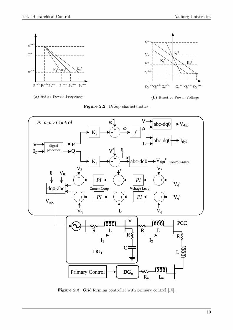
2.4. Hierarchical Control Aalborg Universitet
ωmax
ω*
ωmin
P1min P2
min Pnmin P2
max P1max Pn
max
K1p
K2p Kn
p
(a) Active Power- Frequency
Vmax
Q1min Q2
min Qnmin
K1q
K2q
Knq
Vn
V*
Vmin
Qnmax Q1
max Q2max
(b) Reactive Power-Voltage
Figure 2.2: Droop characteristics.
PCC
R
C
LR
R L
V
DG1
I2I1
R
C
LR
R L
V
DG1
I2I1
DGn
Rn Ln
DGn
Rn Ln
PCC
R
C
LR
R L
V
DG1
I2I1
DGn
Rn Ln
VqVq Iq
Vqc
+-
+-
+-
+-
++
++
PI PI
PIPI
Voltage LoopCurrent Loop
VdVd Id
dq0-abc
θ V0
Vabc
Vqc
+-
+-
+-
+-
++
++
PI PI
PIPI
Voltage LoopCurrent Loop
VdVd Id
dq0-abc
θ V0
Vabc
abc-dq0
abc-dq0
abc-dq0 Control Signal
Kp ʃ
Kq
Vdq0
Idq0
Vdq0c
-+
-+
ω*
V*
ω θ
V
I2V
I2
P
QSignal
processor
V
I2
P
QSignal
processor
V
I2
P
QSignal
processor
abc-dq0
abc-dq0
abc-dq0 Control Signal
Kp ʃ
Kq
Vdq0
Idq0
Vdq0c
-+
-+
ω*
V*
ω θ
V
I2V
I2
P
QSignal
processor
Primary Control
R
L
θ
Vdc
Primary Control
Figure 2.3: Grid forming controller with primary control [15].
10

2.4. Hierarchical Control Aalborg Universitet
R
C
LR
R L
DG1
R
C
LR
R L
DG1
R
C
LR
R L
DG1
R
C
LR
R L
DG2
R
C
LR
R L
DG2
R
C
LR
R L
DG3
R
C
LR
R L
DG3
R
L
R
L
RL LL
RL LL
Load
Load
Load
RL LL
BUS 2
BUS 4
BUS 6BUS 5
BUS 3
BUS 1
Figure 2.4: Single line diagram of test system.
0 0.2 0.4 0.6 0.8 149.9
50
50.1
Fre
qu
ency
[H
z]
0 0.2 0.4 0.6 0.8 1
Time [s]
1950
2000
2050
Act
ive
Po
wer
[W
]
DG1 DG2 DG3
(a) Steady-state
0 0.1 0.2 0.349.9
50
50.1
Fre
qu
ency
[H
z]
0 0.005 0.01 0.015 0.02
Time [s]
0
1000
2000
2600
Act
ive
Po
wer
[W
]
DG1 DG2 DG3
(b) Transient-state
Figure 2.5: Active power share of DGs and system frequency with primary controller.
The control is implemented on a 6-bus system with three DG units given in Figure 2.4. The various
parameters of the system are given in Table 2.1. The active power injected by the DGs and the system
frequency are shown in the Figure 2.5. The reactive power share of all DGs and voltage at load buses
is shown in Figure 2.6. It is observed that due to the same droop gain coefficients of all the DG units,
the active power and reactive power supplied by all the DG units is approx. 1989.5 W and 512 Var.
The controlled DG units maintain stable steady-state condition for the given connected load. However,
there is a steady-state error in the frequency and voltage. This error can be mitigated with the help
11

2.4. Hierarchical Control Aalborg Universitet
0 0.2 0.4 0.6 0.8 1-500
0
500
Volt
age
[V]
0 0.5 1 1.5 2
Time [s]
500
520
540
Rea
ctiv
e P
ow
er [
Var
]
DG1 DG2 DG3
(a) Steady-state
0 0.02 0.04 0.06 0.08 0.1-600
0
600
Vo
ltag
e [V
]
0 0.005 0.01 0.015 0.02
Time [s]
0
200
400
600700
Rea
ctiv
e P
ow
er [
Var
]
DG1 DG2 DG3
(b) Transient-state
Figure 2.6: Reactive power share of DGs and voltage at load buses with primary controller.
of secondary control.
Table 2.1: Parameters for hierarchical control of the given test system.
Parameter Symbol Value UnitNominal Voltage V rms
l−l 400 VNominal frequency f∗ 50 HzFilter Resistance R 0.1 OhmFilter Inductance L 0.0018 HFilter Capacitance C 27× 10−6 FLoad Resistance RL 75.2941 OhmLoad Inductance LL 5.9917× 10⁻² H
Current loop proportional gain Kpc 20 -Current loop integral gain Kic 40 -
Voltage loop proportional gain Kpvo 2.4× 10⁻² -Voltage loop integral gain Kivo 4.5 -
Freq. residual proportional gain Kpw 0.02 -Freq. residual integral gain Kiw 4 -
Voltage residual proportional gain Kpv 0.2 -Voltage residual integral gain Kiv 4 -
Droop coefficient KPn 1.25× 10⁻⁵ -
Droop coefficient KQn 1× 10⁻⁴ -
2.4.2 Secondary control
The secondary control involves in restoring voltage amplitude and frequency deviations in the system.
It measures the frequency and voltage in the microgrid at PCC bus and compares with the references
ω* and |V ∗∗| as shown in Figure 2.7. The error is given to a Proportional-Integral (PI) controller to
obtain the output signals U rw and U rv as shown in (2.3) and (2.4) [17].
12

2.4. Hierarchical Control Aalborg Universitet
R
C
LR
R L
V
DG1
I2I1
R
C
LR
R L
V
DG1
I2I1
DGn
R LDGn
R L
R
C
LR
R L
V
DG1
I2I1
DGn
R L
PCC
Vdq0
Idq0
Vabc-dq0
abc-dq0
abc-dq0
Control Signal
Kp ʃ
Kq Vdq0c
-+
-+
ω*
V*
ω θ
I2V
I2
P
QSignal
processor
V
I2
P
QSignal
processor
V
I2
P
QSignal
processor
+
+
Uvr
Uωr
Vdq0
Idq0
Vabc-dq0
abc-dq0
abc-dq0
Control Signal
Kp ʃ
Kq Vdq0c
-+
-+
ω*
V*
ω θ
I2V
I2
P
QSignal
processor
+
+
Uvr
Uωr
Vdqc
Voltage &
Current Loop
VdqIdq
Vdqc
Voltage &
Current Loop
VdqIdq
Primary Control
Primary
Control
Secondary
Control
V**
VPCC-+
PI
ωPCC-+
PI
V**
VPCC-+
PI
ωPCC-+
PI
Secondary Control
Uωr Uv
r
ω*
R
L
Figure 2.7: Hierarchical control with primary and secondary control.
U rw = Kpw(ω∗ − ωm) +Kiw
∫(ω∗ − ωm) dt (2.3)
U rv = Kpv(|V ∗∗| − |Vm|) +Kiv
∫(|V ∗∗| − |Vm|) dt (2.4)
The gain constants for PI controller are given in the Table 2.1. |Vm| and ωm are the voltage magnitude
and frequency at mth bus (PCC bus). It is noted that Synchronous Reference Frame - Phase Locked
loop (SRF-PLL) measurement is used for secondary frequency control to bring back the system
frequency to the nominal value. The output signals U rw and U rv of PI controllers are sent to primary
control in order to restore the frequency and voltage magnitude. Incorporating these modifications,
the droop equations (2.1) and (2.2) now become,
ω = ω∗ −Kpn.Pn + U rw (2.5)
Vn = V ∗n −Kq
n.Qn + U rv (2.6)
13

2.4. Hierarchical Control Aalborg Universitet
0 0.2 0.4 0.6 0.8 149.9
50
50.1
Fre
qu
ency
[H
z]
0 0.2 0.4 0.6 0.8 1
Time [s]
1950
2000
2050
Act
ive
Po
wer
[W
]
DG1 DG2 DG3
(a) Steady-state
0 0.1 0.2 0.349.9
50
50.1
Fre
qu
ency
[H
z]
0 0.005 0.01 0.015 0.02
Time [s]
0
1000
2000
2600
Act
ive
Po
wer
[W
]
DG1 DG2 DG3
(b) Transient-state
Figure 2.8: Active power share of DGs and system frequency with primary and secondary controller.
0 0.2 0.4 0.6 0.8 1-500
0
500
Vo
ltag
e [V
]
0 0.2 0.4 0.6 0.8 1
Time [s]
500
520
540
Rea
ctiv
e P
ow
er [
Var
]
DG1 DG2 DG3
(a) Steady-state
0 0.02 0.04 0.06 0.08 0.1-600
0
600
Vo
ltag
e [V
]
0 0.005 0.01 0.015 0.02
Time [s]
0
200
400
600700
Rea
ctiv
e P
ow
er [
Var
]
DG1 DG2 DG3
(b) Transient-state
Figure 2.9: Reactive power share of DGs and voltage at load buses with primary and secondarycontroller.
This secondary control is implemented in the test system to compare the results with primary control.
From Figure 2.8 and Figure 2.9 it is observed that there is a slight increase in active power and reactive
power supplied by all the DG units to 2003 W and 515 VAR respectively, as the voltage magnitude
and system frequency are restored to their nominal values with the incorporation of secondary control.
The entire simulink model is illustrated in Figure A.1-A.7 in Appendix A.
2.4.3 Tertiary control
The tertiary level of control adds intelligence to the system in order to optimize the operations of
interest relating to efficiency and economics. It is also known by various other names such as Energy
Management System, Supervisory Control And Data Acquisition, Microgrid Central Controller and
14

2.5. Newton Raphson Power Flow Aalborg Universitet
Microgrid Supervisory Controller [6]. While some papers place EMS into the secondary level and define
tertiary control for multiple microgrid coordination, EMS can also be placed at the tertiary level [6].
EMS can be operated in two control modes: centralized and decentralized [6, 18]. Centralized control
can be used to observe the entire system and is easier to implement. It can be used to optimize the
exchange of power between the microgrid and the grid, or between microgrids. However, the controller
would need to be quite powerful to handle the computational burden and data of the entire system.
Moreover, in case of a fault in the central control unit, the entire system is susceptible to failure.
Decentralized control addresses these shortcomings, however it has drawbacks of its own. Although it
offers more flexibility in operation and avoids a single point of failure, a decentralized control scheme
requires high level of coordination and synchronization between the units along with a communication
system. Moreover, it may also compromise security of the system. Thus, depending on the size and
purpose of the microgrid, a suitable scheme is used [6, 18]. However, irrespective of the type of control,
the main duty of an EMS is to ensure reliable system operation.
An EMS involves one or more decision making algorithms, trying to optimize objectives of interest
under various constraints [19]. The tertiary control operates in the order of several minutes, hence its
output is considered as constant for power flow modelling, which operates in the order of few seconds
[4]. An extensive survey of different optimization objectives, algorithms, and constraints have been
discussed in [18, 19]. Some of these objectives include minimizing CO2 emissions, maximize RES share,
maximize profits etc. subject to constraints such as ESS storage capacity, generation limits, voltage
at buses, system frequency, among others.
2.5 Newton Raphson Power Flow
The Newton-Raphson (NR) method is a well-known iterative algorithm for root-finding. Since power
flow is a non-linear algebraic problem, it can be solved using the NR method [20, 21]. The general
equation for NR method for a function F (x) with jacobian J and change in variable ∆x, and the
update equation for the kth iteration are given in (2.7) and (2.8) respectively.
F (x)k = −Jk∆xk (2.7) xk+1 = xk + ∆xk (2.8)
The NR method aims to minimize the power mismatch equations in vector F (x) given in (2.9) in order
to estimate the change in the system variables ∆x i.e., the bus voltage magnitudes |Vn| and angles δn.
F (x) =
∆Pn = P(scheduled)n − P (calculated)
n
∆Qn = Q(scheduled)n −Q(calculated)
n
(2.9)
where the scheduled power is the difference between total generation and total load at that bus, and
15

2.5. Newton Raphson Power Flow Aalborg Universitet
calculated powers are given by [20, 21],
P (calculated)n =
N∑i=1
|Vn||Vi||Yni|cos(θni + δi − δn) for n = 1, ..., N (2.10)
Q(calculated)n = −
N∑i=1
|Vn||Vi||Yni|sin(θni + δi − δn) for i = n, ..., N (2.11)
Conventionally, NR power flow is solved by reducing the partial differential equations in the Jacobian
J to a set of algebraic equations [20, 21].
2.5.1 Power Flow in Microgrids
The conventional power flow problem is formulated by categorizing each bus into one of the following
three types: Generator or PV Bus, Load or PQ Bus, and Slack Bus. However, for islanded microgrids
a different approach for categorizing the buses is necessary.
2.5.1.1 Primary Control
The conventional power flow methodology cannot be used for microgrids due to the following reasons
[22, 23]:
1. The frequency in an islanded AC microgrid is constantly varying and cannot be assumed to be
fixed.
2. A slack bus cannot be defined since the DGs have limited capacities.
3. The sharing of active and reactive power among the DGs, and the local bus voltages, are not
pre-specified and hence, the buses cannot be simply categorised as PQ or PV bus. Moreover,
power sharing among the DGs depends on their droop characteristics.
Therefore, a new type bus categorisation is introduced, vis-a-vis Droop Bus [23, 24]. The Droop Bus
is defined by the droop equations (2.1) and (2.2), which are used to calculate the scheduled active and
reactive powers for a droop controlled DG. These scheduled power are as follows,
P (scheduled)n =
ω∗ − ωKpn
(2.12) Q(scheduled)n =
V ∗n − VnKqn
(2.13)
Moreover, since the frequency of the microgrid is not constant, a relation for the system frequency is
also required. This is achieved by fixing the voltage angle of one of the DGs as reference and adding its
active power droop equation (2.1) to the formulation as separate relation [25]. This frequency relation
is used to estimate the per unit frequency of the system. The final formulation of the power mismatch
vector with Droop Buses is as follows,
16

2.5. Newton Raphson Power Flow Aalborg Universitet
∆Pn
∆Qn
∆w
=
P
(scheduled)n − P (calculated)
n
Q(scheduled)n −Q(calculated)
n
(ω∗ − ω)− (KpnP
(calculated)n )
(2.14)
The power flow can be solved numerically using the NR method. However, to simulate a more realistic
power flow the effect of both primary and secondary controls are required.
2.5.1.2 Secondary Control
Droop controlled buses, i.e., the Droop Bus, does not represent a DG unit with secondary controls for
voltage and frequency restoration. Therefore, a different formulation is required for the inclusion of
secondary control [24].
Frequency Restoration
The active power Pn of a DG unit with secondary control is given by (2.5). In steady state, the system
frequency ω is equal to the reference frequency ω∗. Thus, from (2.3) and (2.5), the scheduled active
power for the n-th DG can be given by,
P (scheduled)n =
U intw
Kpn
(2.15)
where U intw is the integral part of U rn from (2.3) in steady state.
The bus phase angle δm where secondary control is required to regulate the voltage and frequency is
given as follows,
θm = ω∗t+ δm (2.16)
where θm is the reference frame angle and t is time. On differentiating (2.16),
dθmdt
= ωm = ω∗ +dδmdt
ordδmdt
= ωm − ω∗(2.17)
Substituting (2.17) in (2.3), the relation for U intw becomes as follows,
U intw = −Kiw
∫dδmdt
dt = −Kiw(δm − δ0m) (2.18)
where δ0m is the initial condition. Hence, the equation for scheduled active power (2.15) becomes [24],
P (scheduled)n =
−Kiw(δm − δ0m)
Kpn
(2.19)
Here, δm is the angle of the bus being controlled by secondary frequency control. The control sets the
reference phase angle for all the DG units and thus, there is no need to fix a bus angle as reference, as
was the case in primary control [25].
17

2.5. Newton Raphson Power Flow Aalborg Universitet
Voltage Restoration
The relation for scheduled reactive power for the n-th DG unit, based on (2.4) and (2.6) is as follows,
Q(scheduled)n =
|V ∗n | − |Vn|+ U rv
Kqn
(2.20)
Since, in steady state, the voltage magnitude of the bus being controlled by secondary control will
be 1 pu, i.e., |Vn| = |V ∗∗| therefore, U rv = U intv . Moreover, this also implies that the reactive power
equation for this bus is not being used in the formulation since the result is already fixed, i.e., voltage
is already known. Instead, this equation can be used to estimated U intv , which cannot be calculated in
any other way, as was the case for U intw [24]. This way the reactive power equation for the bus being
controlled is still used in the formulation. Thus, U intv , becomes one of the variable to estimate by NR
iterations, along with the bus voltages and angles.
This new bus type based on (2.19) and (2.20) is called the Hierarchically Controlled PQ (HCPQ) Bus
and includes the effects of both primary and secondary controls [24]. The power mismatch vector can
hence be formulated as follows,
F (x) =
∆Pn
∆Qn
=
P (scheduled)n − P (calculated)
n
Q(scheduled)n −Q(calculated)
n
(2.21)
The 6-bus system studied in 2.4 with three DGs is simulated in MATLAB for two cases: i) with
primary controlled Droop Bus and ii) with primary and secondary controlled HCPQ Bus. The results
are compared in Table 2.2. Since the system is symmetrical and balanced, all DGs will generate the
same output and the same voltage will be observed at all three loads.
As it can be seen from Table 2.2, with the inclusion of secondary control, the bus voltage magnitude
and the system frequency are restored to their nominal values. Moreover the results from MATLAB
simulation match with those from the Simulink simulation in 2.4. However, the NR power flow
simulations do not consider operational constraints of the DG units, nor does it factor in any
optimization objective.
Table 2.2: Comparison of MATLAB simulation for hierarchical power flow.
Parameter Case i) Case ii)
Bus Voltage Magnitude[p.u.] DG 0.9999 1.0030Load 0.9968 1.0000
Bus Voltage Angle [degrees] DG 0 0.274Load -0.3859 -0.3586
Active Power [W] DG 1990 2003Reactive Power [VAR] DG 512 515System Frequency [Hz] 49.9960 50.0000
18

2.6. Economic Dispatch Aalborg Universitet
2.6 Economic Dispatch
The ever-varying electric load demand is required to be met by the power generating units in the
network in order to maintain power balance in the system. However, CG units vary widely in their
operational cost and capacity. Fossil-fired units with a low marginal cost are relatively inflexible and
the generators that can follow the load tend to be more expensive. The generators are also subjected
to fuel limitations and environmental regulations that restrict their availability. These characteristics
of the CG units are undertaken by the economic optimization process called ED [26].
~||
~||
Load ~||
~||
Conventional
Generators
Battery
Energy
Storage
Systems
Power
Communication
Power
Communication
Economic
Dispatch
~~~
Wind
Turbines
Figure 2.10: Schematic representation of the test system for ED.
ED aims to schedule the power outputs of the available generating units in such a way that operation
cost of the generating units is minimized, while satisfying system constraints [26]. The other objectives
of ED are as follows,
• Scheduling the committed generation units outputs to meet the required load while satisfying all
units and system equality and inequality constraints with minimum operating cost.
• Minimizing the CO2 emissions of CGs.
• Minimizing the losses in the system.
• Profit maximization by reducing the total cost.
• Maintaining system stability and security constraints.
In this section, the ED of active power generation is considered for a system with four CG units, one
WT and a BESS. A schematic representation of the system is illustrated in Figure 2.10.
19

2.6. Economic Dispatch Aalborg Universitet
The cost function for ED is modelled as follows [27],
minPg
TH∑t=1
NG∑g=1
(agP2g (t) + bgPg(t) + cg)
subject to,NG∑g=1
Pg(t)− PL(t) = 0
Pming − Pg(t) ≤ 0
Pg(t)− Pmaxg ≤ 0
(2.22)
where TH is the time horizon, NG is the number of CGs, Pg is the power generated by DGs, Pming and
Pmaxg are the CG’s operating limits, PL(t) is the load at time instant t, and ag [$/kW 2], bg [$/kW ]
and cg [$] are the cost coefficients, given in Table 2.3.
However, there may be other objective functions which may need to be satisfied instead of operational
cost, such as minimizing environmental impact or minimizing losses in the system. Moreover, in
a practical power system multiple objectives may need to be optimized together, with different
weights showing the priorities given to each objective function. The emission function for minimizing
environmental impact is given as follows [27],
minPg
TH∑t=1
NG∑g=1
(dgP2g (t) + egPg(t) + fg)
subject to,NG∑g=1
Pg(t)− PL(t) = 0
Pming − Pg(t) ≤ 0
Pg(t)− Pmaxg ≤ 0
(2.23)
where dg [kg/kW 2], eg [kg/kW ] and fg [kg] are the emission coefficients, given in Table 2.3. The
multiobjective optimization problem for simultaneous minimization of operational cost and emission
is given below in (2.24) with weights w1 and w2.
minPg
w1
TH∑t=1
NG∑g=1
(agP2g (t) + bgPg(t) + cg)
+ w2
TH∑t=1
NG∑g=1
(dgP2g (t) + egPg(t) + fg)CGemission
for weights, w1 ∈ [0, 1] and w2 = 1− w1
(2.24)
20

2.6. Economic Dispatch Aalborg Universitet
Table 2.3: List of coefficients and constraints for operational cost and emission functions [27].
g ag[$/MW 2]
bg[$/MW ]
cg[$]
dg[kg/MW 2]
eg[kg/MW ]
fg[kg]
Pming
[MW ]
Pmaxg
[MW ]
RUg[MW ]
RDg
[MW ]
1 0.12 14.8 89 1.2 -5 3 28 200 40 402 0.17 16.57 83 2.3 -4.24 6.09 20 290 30 303 0.15 15.55 100 1.1 -2.15 5.69 30 190 30 304 0.19 16.21 70 1.1 -3.99 6.2 20 260 50 50
The parameter CGemission is the environmental emission cost and is needed to convert the emission
function (2.23) to the same units as the operational cost function (2.22). It’s value is 0.1 $/kg [27].
The multiobjective function is solved in MATLAB using the fmincon function for one hour for a load
value of 510 MW. The results are given in Table 2.4. As expected, the operational cost and emission
values vary with the change in weights, with the maximum cost (and minimum emission) incurring at
w1 = 0 and the minimum cost (and maximum emission) at w1 = 1.
Table 2.4: Comparison of results for different weights for multiobjective ED with operational costand emission functions.
w1 w2 P1[MW] P2[MW] P3[MW] P4[MW] Cost[$] Emission[kg]0 1 138.22 71.95 149.49 150.33 19160.37 82380.23
0.25 0.75 147.79 81.32 146.12 134.77 18732.37 82970.870.50 0.50 155.52 91.01 141.57 121.90 18469.25 84532.650.75 0.25 161.63 101.20 136.27 110.90 18325.88 86906.991 0 166.19 112.11 130.45 101.25 18280.38 90075.55
Ramp Rates
A practical CG unit would also have mechanical limitations and cannot suddenly increase or decrease
generation output. Hence, constraints on ramping the generation up and down are necessary. On
including the ramp-up rate RUg and ramp-down rate RDd, the optimization problem becomes,
minPg
TH∑t=1
NG∑g=1
(agP2g (t) + bgPg(t) + cg)
subject to,NG∑g=1
Pg(t)− PL(t) = 0
Pming − Pg(t) ≤ 0
Pg(t)− Pmaxg ≤ 0
Pg(t+ 1)− Pg(t)−RUg ≤ 0
Pg(t)− Pg(t+ 1)−RDg ≤ 0
(2.25)
The objective function given in (2.25) was solved for a time horizon of 24 hours using the load data
given in Table 2.5. The calculated operational cost was found to be $ 647,964.46 and the corresponding
21

2.6. Economic Dispatch Aalborg Universitet
emission at that operational cost was 3,592,886.72 kg.
Table 2.5: Load data [27] for operational cost optimization.
Time (t) Load (PL) Time (t) Load (PL)[hr] [MW] [hr] [MW]1 510 13 7542 530 14 7003 516 15 6864 510 16 7205 515 17 7146 544 18 7617 646 19 7278 686 20 7149 741 21 61810 734 22 58411 748 23 57812 760 24 544
1 2 3 4 5 6 7 8 9 10 11 12 13 14 15 16 17 18 19 20 21 22 23 24
Time [hr]
100
125
150
175
200
Po
wer [
MW
]
DG 1 DG 2 DG 3 DG 4
Figure 2.11: Active power generation of CGs for operational cost optimization.
1 2 3 4 5 6 7 8 9 10 11 12 13 14 15 16 17 18 19 20 21 22 23 24
Time [hr]
500
600
700
800
Po
wer
[M
W]
Total Generation
Hourly Demand
Figure 2.12: Power balance for operational cost optimization.
The active power generation of all four CGs for the optimized operational cost is displayed in
Figure 2.11. It is observed that CG1 contributes more than the other CGs. This is due to the
fact that CG1 is the cheapest to operate due to its cost coefficients. From Figure 2.12 it can be seen
that power balance is obtained as the total generation is equal to the total load demand for every hour.
Storage System
A storage system is an essential component in a microgrid, as also briefly discussed in 2.1 and 2.3.
In order to include a BESS in the system, the battery constraints are required to be included in the
optimization formulation. These constraints are,
22

2.6. Economic Dispatch Aalborg Universitet
• BESS charging (Pc) and discharging (Pd) limits.
• The State of Charge (SOC) limits.
• Calculation of present SOC based on previous SOC and BESS parameters such as battery
capacity (E), charging or discharging power and efficiency (η).
• Including the power charged or discharged by the BESS in the power balance equality constraint.
• The BESS should have a set amount of SOC (SOC0) at the end of the time horizon for the next
day.
Table 2.6: Parameters for BESS [27]
Parameter Value UnitSOC0 0.25 -SOCmin 0.2 -SOCmax 0.8 -Pmind 0 MWPmaxd 60 MWPminc 0 MWPmaxc 60 MWηd 90 %
ηc 95 %
E 400 MWh
23

2.6. Economic Dispatch Aalborg Universitet
On incorporating these constraints, the optimization problem now becomes as follows,
minPg Pd Pc SOC
TH∑t=1
NG∑g=1
(agP2g (t) + bgPg(t) + cg)
subject to,NG∑g=1
Pg(t) + Pd(t)− PL(t)− Pc(t) = 0
SOC(t)− SOC(t+ 1) +1
E(ηcPc −
1
ηdPd)∆t = 0
SOC(TH)− SOC0 = 0
Pming − Pg(t) ≤ 0
Pg(t)− Pmaxg ≤ 0
Pg(t+ 1)− Pg(t)−RUg ≤ 0
Pg(t)− Pg(t+ 1)−RDg ≤ 0
SOCmin − SOC(t) ≤ 0
SOC(t)− SOCmax ≤ 0
Pmind − Pd(t) ≤ 0
Pd(t)− Pmaxd ≤ 0
Pminc − Pc(t) ≤ 0
Pc(t)− Pmaxc ≤ 0
(2.26)
The BESS parameters are given in Table 2.6. On solving the updated operational cost function with
BESS given in (2.26), the total operational cost was reduced to $ 645497.74 and the total emission
at this cost decreased to 3,558,071.32 kg. Figure 2.13, 2.14 and 2.15 illustrate the change in BESS
SOC, BESS power, and the active power generation of the CGs respectively. As seen from Figure 2.16,
power balance is maintained in the system.
2 4 6 8 10 12 14 16 18 20 22 24
Time [hr]
0
0.2
0.4
0.6
0.8
1
BE
SS
SO
C
Figure 2.13: Normalized SOC of BESS.
2 4 6 8 10 12 14 16 18 20 22 24
Time [hr]
-60
-30
0
30
60
BE
SS
Po
wer
[M
W]
Discharge
Charge
Figure 2.14: BESS power for 24 hours.
24

2.6. Economic Dispatch Aalborg Universitet
1 2 3 4 5 6 7 8 9 10 11 12 13 14 15 16 17 18 19 20 21 22 23 24
Time [hr]
100
150
200
Po
wer [
MW
]
DG 1 DG 2 DG 3 DG 4
Figure 2.15: Active power generation of DGs for operational cost optimization with BESS.
1 2 3 4 5 6 7 8 9 10 11 12 13 14 15 16 17 18 19 20 21 22 23 24
Time [hr]
0
200
400
600
800
Po
wer
[M
W]
DG BESS Discharge Load BESS Charge
Figure 2.16: Active power balance for operational cost optimization with BESS.
RES generation curtailment
RES integration in microgrid is discussed in 2.3. Needless to say, the RES penetration should be
maximized in order to have the least environmental footprint and fuel cost. Therefore, the inclusion
of RES such as WT in the optimization problem should intend to minimize its curtailment. This is
achieved by introducing a penalty factor CWT for the curtailed wind power PWTc. The available wind
power is given in Table 2.7.
Table 2.7: Available wind power data [27].
Time (t) Available wind Time (t) Available wind[hr] power (PWT ) [MW] [hr] power (PWT ) [MW]1 44.1 13 487.62 48.5 14 521.93 65.7 15 541.34 144.9 16 5605 202.3 17 486.86 317.3 18 372.67 364.4 19 367.48 317.3 20 314.39 271 21 316.610 306.9 22 311.411 424.1 23 405.412 398 24 470.4
The optimization problem is thus modified as follows,
25

2.6. Economic Dispatch Aalborg Universitet
minPg Pd Pc SOC PWTc
TH∑t=1
NG∑g=1
(agP2g (t) + bgPg(t) + cg) +
TH∑t=1
(PWTc CWT )
subject to,NG∑g=1
Pg(t) + Pd(t) + PWT (t)− PL(t)− Pc(t)− PWTc(t) = 0
SOC(t)− SOC(t+ 1) +1
E(ηcPc −
1
ηdPd)∆t = 0
SOC(TH)− SOC0 = 0
Pming − Pg(t) ≤ 0
Pg(t)− Pmaxg ≤ 0
Pg(t+ 1)− Pg(t)−RUg ≤ 0
Pg(t)− Pg(t+ 1)−RDg ≤ 0
SOCmin − SOC(t) ≤ 0
SOC(t)− SOCmax ≤ 0
Pmind − Pd(t) ≤ 0
Pd(t)− Pmaxd ≤ 0
Pminc − Pc(t) ≤ 0
Pc(t)− Pmaxc ≤ 0
PWTc − PWT ≤ 0
− PWTc ≤ 0
(2.27)
where PWT is the available power output of WT at time t, given in Table 2.7 and the penalty factor
CWT = 50 $/MW [27]. On solving, the optimized operational cost was found to be $ 226511.14 and
the total emission at this cost was 891353.03 kg. The inclusion of WT reduces operational cost by
64.91 % and emission at those costs by 74.95 %, as compared to the case with only BESS. Clearly, the
inclusion of WT complements the optimization objective of minimizing operational cost, along with
reducing the environmental impact of the system.
From Figure 2.17 and 2.19 it can be inferred that the BESS and WT complement the optimization
objective in minimizing operational cost by reducing the CG generation output. Figure 2.20 illustrates
that there is no wind curtailment. As observed from Figure 2.21, power balance is maintained
throughout the time horizon with the help of BESS and WT.
At t = 24 wind generation is high. Subsequently, the CGs are pushed down to their minimum
operational limits in order to minimize cost. After meeting the load demand, the excess power should
26

2.6. Economic Dispatch Aalborg Universitet
1 2 3 4 5 6 7 8 9 10 11 12 13 14 15 16 17 18 19 20 21 22 23 24
Time [hr]
0
0.2
0.4
0.6
0.8
1
BE
SS
SO
C
Figure 2.17: Normalized SOC with WT.
2 4 6 8 10 12 14 16 18 20 22 24
Time [hr]
-60
-30
0
30
60
BE
SS
Po
wer
[M
W]
Discharge
Charge
Figure 2.18: BESS power with WT.
1 2 3 4 5 6 7 8 9 10 11 12 13 14 15 16 17 18 19 20 21 22 23 24
Time [hr]
0
50
100
150
Po
wer [
MW
]
DG 1 DG 2 DG 3 DG 4
Figure 2.19: Active power generation of CGs for operational cost optimization with BESS and WT.
1 2 3 4 5 6 7 8 9 10 11 12 13 14 15 16 17 18 19 20 21 22 23 24
Time [hr]
0
200
400
600
Po
wer [
MW
]
Curtailed
Available
Figure 2.20: Available wind power and curtailment.
be used to charge the BESS. At this hour, the BESS needs to have exactly 25% SOC. However, from
the Figure 2.18 it can be seen that both charging and discharging action of BESS take place at this
hour. The optimization solver considers this as the mathematically feasible solution, even though this
is not a practically feasible solution. A reason for this is that there is no explicit constraint that
27

2.6. Economic Dispatch Aalborg Universitet
1 2 3 4 5 6 7 8 9 10 11 12 13 14 15 16 17 18 19 20 21 22 23 24
Time [hr]
0
200
400
600
800
1000
1200
Po
wer
[M
W]
DG
BESS Discharge
Available Wind Power
Load
BESS Charge
Curtailed Wind Power
Figure 2.21: Active power balance for operational cost optimization with BESS and WT.
prevents both charging and discharging to occur simultaneously. To overcome this problem, the SOC
constraint for t = 24 in the equation 2.27 is modified as follows,
SOC0 − SOC(TH) ≤ 0 (2.28)
1 2 3 4 5 6 7 8 9 10 11 12 13 14 15 16 17 18 19 20 21 22 23 24
Time [hr]
-60
-40
-20
0
20
40
60
BE
SS
Po
wer
[M
W]
Discharge
Charge
Figure 2.22: BESS power with WT (SOC(TH) ≥ SOC0).
From Figure 2.22 it can be seen that although there is still an existence of the discharging power of
BESS, its value is greatly reduced. To further verify this BESS behaviour, the load at t = 24 is varied
and the results for that hour are shown in Table 2.8,
From Table 2.8 it can be inferred that the BESS has certain amount of discharging power, when there
is no wind power curtailment and the power generated by the CGs reach to their minimum value. In
order to resolve this anomaly, one of the following things may be done,
• Introduce a binary variable to signify when to charge or discharge. However this would convert the
optimization problem into a Mixed Integer type problem. That would require a more advanced
solver since the problem would become more complex.
• Both charging and discharging can be represented by a single variable. Moreover, the charging
and discharging efficiencies are assumed to be 100%.
28

2.6. Economic Dispatch Aalborg Universitet
• Add a cost for BESS operation. This would prevent simultaneous charging and discharging action
since both operations would add to the cost. This might, however, decrease the BESS usage.
• A non-linear constraint could be included which requires the product of the charging and
discharging power to be zero at all hours.
Table 2.8: Results at t=24 with different load values.
Pg1 Pg2 Pg3 Pg4 Pd Pc SOC PWTc Load[MW] [MW] [MW] [MW] [MW] [MW] [MW] [MW]28 20 30 20 0.85 25.25 0.257 0 544
51.65 31.25 38.82 28.91 0 21.05 0.25 0 60038.31 21.84 30 20.49 0 21.05 0.25 0 56028 20 30 20 0.64 23.04 0.25 0 54628 20 30 20 1.62 30.02 0.26 0 54028 20 30 20 0 60 0.342 8.4 500
By employing the second procedure and assuming ideal behaviour of BESS, the SOC-Power relation
given in (2.26) is modified as shown in (2.29), which is implemented in chapter 3. Note, that the BESS
charging power is taken as negative and discharging power is taken as positive.
SOC(t+ 1) = SOC(t) +−PBESS
E∆t (2.29)
Load Shedding
Load shedding is discussed in 2.2. The implementation of load shedding in the optimization problem
is performed to minimize the operational cost and emission from CGs, when the RES generation may
not be sufficient to meet the required demand. This, however, is done by introducing a penalty factor
for the shed load called Value of Loss of Load (VOLL) which is assumed to be 50 $/MW . Thus,
there is a trade-off between increasing the cost due to the load shedding penalty and decreasing the
operational cost from CGs. The optimization problem is modified as follows,
29

2.6. Economic Dispatch Aalborg Universitet
minPg Pd Pc SOC PWTc PLS
TH∑t=1
NG∑g=1
(agP2g (t) + bgPg(t) + cg) +
TH∑t=1
(PWTc CWT + PLS V OLL)
subject to,NG∑g=1
Pg(t) + Pd(t) + PLS + PWT (t)− PL(t)− Pc(t)− PWTc(t) = 0
SOC(t)− SOC(t+ 1) +1
E(ηcPc −
1
ηdPd)∆t = 0
SOC(TH)− SOC0 = 0
Pming − Pg(t) ≤ 0
Pg(t)− Pmaxg ≤ 0
Pg(t+ 1)− Pg(t)−RUg ≤ 0
Pg(t)− Pg(t+ 1)−RDg ≤ 0
SOCmin − SOC(t) ≤ 0
SOC(t)− SOCmax ≤ 0
Pmind − Pd(t) ≤ 0
Pd(t)− Pmaxd ≤ 0
Pminc − Pc(t) ≤ 0
Pc(t)− Pmaxc ≤ 0
PWTc − PWT ≤ 0
− PWTc ≤ 0
PLS − PL ≤ 0
− PLS ≤ 0
(2.30)
where PLS is the total load shed at time t. On solving, the optimized operational cost was found to be $
226482.68 and the total emission at this cost was 878233.92 kg. The inclusion of WT and load shedding
reduces the operational cost by 64.91 % and emission at those costs by 75.31 %, as compared to the
case with only BESS. The addition of load shedding with WT and BESS further complements the
optimization objective of minimizing operational cost, along with reducing the environmental impact
of the system.
Figure 2.23, 2.24 and 2.25 shows the changes in BESS SOC, BESS power, and the active power
generation of the CGs respectively. From the Figure 2.24 it can be seen that both charging and
discharging action of BESS take place at t=24. This problem can be resolved by following one of the
30

2.6. Economic Dispatch Aalborg Universitet
four possibilities as discussed in the previous section with ED with BESS and WT in 2.6.
2 4 6 8 10 12 14 16 18 20 22 24
Time [hr]
0
0.2
0.4
0.6
0.8
1
BE
SS
SO
C
Figure 2.23: Normalized SOC with WT andload shedding.
2 4 6 8 10 12 14 16 18 20 22 24
Time [hr]
-60
-30
0
30
60
BE
SS
Pow
er [
MW
]
Discharge
Charge
Figure 2.24: BESS power with WT and loadshedding.
1 2 3 4 5 6 7 8 9 10 11 12 13 14 15 16 17 18 19 20 21 22 23 24
Time [hr]
0
50
100
150
Po
wer [
MW
]
DG 1 DG 2 DG 3 DG 4
Figure 2.25: Active power of CGs for operational cost optimization with BESS, WT and loadshedding.
1 2 3 4 5 6 7 8 9 10 11 12 13 14 15 16 17 18 19 20 21 22 23 24
Time [hr]
0
200
400
600
800
Po
wer
[M
W]
Curtailment
Load shedding
Total load
Total wind power
Figure 2.26: Load shedding and wind curtailment.
1 2 3 4 5 6 7 8 9 10 11 12 13 14 15 16 17 18 19 20 21 22 23 24
Time [hr]
0
200
400
600
800
1000
1200
Po
wer
[M
W]
CG
BESS Discharge
Available Wind Power
Load shedding
Load
BESS Charge
Curtailed Wind Power
Figure 2.27: Active power balance for operational cost optimization with BESS, WT and loadshedding.
From the Figure 2.26 it is observed that the load shedding takes place at the instances where difference
31

2.7. Summary Aalborg Universitet
in load and available RES power is high, in order to minimize the operating cost of CGs. As seen from
Figure 2.27, power balance is maintained in the system with inclusion of load shedding.
2.7 Summary
This chapter describes the basic hierarchical control scheme of islanded AC microgrid that ensures
safety, reliability and economic benefits. The primary and secondary controls are explained with
schematic diagrams. The control behaviour is analyzed using a 6-bus test system. Additionally,
steady-state analysis of islanded AC microgrid is solved numerically using the NR method. Moreover,
to simulate a realistic microgrid power flow, the effect of primary and secondary control is considered.
Thus, droop-based extended power flow and hierarchical extended power flow are performed. For each
method, the power flow formulation is explained and the results for the modelled system are presented.
The steady-state solution obtained from the power flow, however, does not consider ED i.e., as cost of
operation of different CGs, operating limitations of CGs, losses, etc [20]. In a practical power system,
these constraints are required to be included in the problem formulation while optimizing the power
flow solution. To achieve this objective, the Extended Optimal Power Flow (EOPF) is introduced in
Chapter 3.
32

3 | Extended Optimal Power Flow
3.1 Introduction
A power system optimization problem that contains the power flow equations (2.10) and (2.11) may
be classified as an Optimal Power Flow (OPF) problem [28]. The aim of OPF is to optimize a given
objective by controlling the power flow, while making sure that the system components operate within
their constraints and operating limits.
In islanded AC microgrids, the DGs also need to regulate the voltage and frequency in the system,
apart from supplying power to meet the demand [29]. For this purpose, power flow-based hierarchical
schemes have been proposed in literature, specifically droop-based methods. The inclusion of power
flow inside the optimization automatically ensures power balance, rather than having a power balance
constraint. A droop-based method for load sharing and voltage regulation is described in [30]. In [31],
a HC power flow optimization is presented for loss minimization and ensuring frequency stability in the
islanded microgrid. These hierarchical-based methods regulate the bus voltage and system frequency,
and ensure power balance while optimizing a higher level objective.
A real-time centralized Extended Optimal Power Flow (EOPF) control is proposed in [32] which
uses the droop bus formulation from 2.5.1.1 to optimize active and reactive power sharing (%)
among the DGs in the microgrid, along with maintaining PCC voltage and maximizing the microgrid
efficiency. The optimization is activated when a change in load or generation capacity is detected.
The control dynamics of each participating DG is taken into account and thus, their droop coefficients
are optimized. These optimized droop coefficients (Kpn and Kq
n) define the dynamic and steady state
operation of the DG units.
In droop bus formulation, each generation unit uses frequency instead of phase angle to control the
active power flow since the initial phase angle values of other generation units are not known [33].
However, the initial frequency can be easily fixed as ω∗ at no-load condition. This results in a trade-
off between active power sharing and frequency accuracy in system [33]. Furthermore, the DGs are
connected to the system through long feeders and are located far from the load. This may lead to
voltage quality issues, reactive power flow, and power losses [32]. These problems can be resolved by
HCPQ bus formulation. This technique represents DG units with secondary control for voltage and
frequency restoration. Therefore, frequency and voltage restoration objectives need not be included
33

3.2. EOPF Algorithm with HCPQ Bus Aalborg Universitet
in the EOPF formulation. It can be assumed that the microgrid frequency and reference bus voltages
are regulated to 1 p.u. The inclusion of both primary and secondary controls inside the optimization
would make the dynamics of the microgrid more realistic. This algorithm is explained in the subsequent
section.
3.2 EOPF Algorithm with HCPQ Bus
An EMS is a tertiary level control that supervises the operation of a microgrid, as explained in 2.4.3.
The controlling algorithm in the EMS has the function of optimizing the objectives of interest while
maintaining optimal operating conditions in the system.
The primary level dynamics of a DG depend on its droop characteristics. Hence, in order to control
the steady state performance of a DG , the droop characteristics of a DG need to be controlled [32],
i.e., the droop coefficients need to be optimized. Furthermore, as elaborated in 2.5.1.2, the HCPQ bus
formulation is able to restore the system frequency and bus voltages to well within the operational
limits. Thus, if the HCPQ bus formulation regulates the system frequency and bus voltages, the droop
characteristic can be controlled in order to achieve a higher level objective. In this way, an EOPF
algorithm with HCPQ bus is proposed in Figure 3.1, which is inspired by the work in [32].
The algorithm works as follows,
1. A set of variables are initialized, which are to be optimized. These include the droop coefficients,
along with other parameters depending upon the optimization objective and components in the
system.
2. A steady state solution is found using the initialized variables by using HCPQ bus formulation.
3. The optimization problem is solved, subject to 0.
4. If an optimal solution is not reached, a new set of optimization variable are taken and the process
is repeated from step 2.
5. If an optimal solution is achieved, the optimization process ends.
This algorithm is used in the following sections for different optimization objectives, using the 6-bus
microgrid from Figure 2.4.
1. Equal power sharing (%) among the DGs.
2. Cost Minimization
3. Cost minimization, with the inclusion of an ideal BESS.
4. Cost minimization, with the inclusion of load shedding constraints.
34

3.2. EOPF Algorithm with HCPQ Bus Aalborg Universitet
Start
Initialize
optimization
variables
Compute steady state
extended power flow
solution with HCPQ Bus
Compute
optimization
objective function
Optimal solution
achieved?
New set of
optimization
variables
End
Yes
No
Figure 3.1: Proposed EOPF algorithm with HCPQ bus.
The simulations are performed on a computer with processor Intel (R) Core (TM) i5 - 8250U CPU @
1.60 GHz, 1800 MHz with 8 GB RAM.
3.2.1 Power Sharing
In equal power sharing, each DG unit operates at the same percentage of its maximum capacity. Power
sharing among DGs in a microgrid is important so as to share the load burden equally. In order to
compute the optimal droop characteristics of each DG unit, the power sharing optimization problem
is modelled as follows,
minKp
n Kqn
TH∑t=1
NG∑g=1
NG∑k=1
( Pg(t)
Smaxg (t)− Pk(t)
Smaxk (t)
)2+( Qg(t)
Smaxg (t)− Qk(t)
Smaxk (t)
)2
subject to, Kq minn −Kq
n ≤ 0
Kqn −Kq max
n ≤ 0
Kp minn −Kp
n ≤ 0
Kpn −Kp max
n ≤ 0
(3.1)
35

3.2. EOPF Algorithm with HCPQ Bus Aalborg Universitet
The power sharing objective function is modelled as the sum of least squared errors between the active
and reactive power share (%) of the different DG units. The active (Pg and Pk) and reactive (Qg and
Qk) powers are calculated by the power flow equations of HCPQ bus described in 2.5.1.2. Smaxg is
maximum apparent power capacity of the respective DG unit.
The optimization problem in (3.1) was simulated in MATLAB using fmincon function for t= 1 for the
6 bus test system in Figure 2.4 and the results are tabulated below in Table 3.1. As it can be seen,
the DG units generate an equal share (%) of active and reactive powers, based on their capacities.
The bus voltage magnitudes and angles are shown in Table 3.2. The simulation ran for 29 iterations
and took 4.96 seconds, and the objective function (least squared error) was minimized to 3.05 × 10⁻⁸.
The DG capacities are also given in Table 3.1. The limits for droop coefficients were as follows:
0.25 × 10⁻⁵ ≤ Kpn ≤ 6.25 × 10⁻⁵ and 2 × 10⁻⁷ ≤ Kq
n ≤ 5 × 10⁻². It is to be noted that these limits
and capacities are arbitrary and do not represent any real system, they are only to test the simulation
algorithm.
Table 3.1: Results for EOPF for active and reactive power sharing among DG units.
Pg [W] Pg Share [%] Knp Qg [VAR] Qg Share [%] Kn
q Sgmax [VA]
DG1 2255.94 75.20 2.3939e-5 580.64 19.35 0.0189 3000DG2 2255.86 75.20 2.3940e-5 581.08 19.37 0.0109 3000DG3 1504.01 75.20 3.5907e-5 387.79 19.39 0.0305 2000
Table 3.2: Bus voltage and angle for EOPF power sharing.
Bus Voltage [p.u.] Angle [degrees]1 1.0045 -0.19562 1.0011 -0.63923 1.0042 -0.24334 1.0007 -0.67725 1.0023 -0.48366 1.0000 -0.7736
3.2.2 Cost Minimization
In this, and the subsequent sections, the cost minimization EOPF problem is simulated for a time
horizon of 24 hr for the same 6-bus system in Figure 2.4. First, a base case is performed in this
section. The next two cases observe an addition of a BESS and load shedding constraints respectively.
The optimization problem is modelled as shown in (3.2).
36

3.2. EOPF Algorithm with HCPQ Bus Aalborg Universitet
minKp
n Kqn
TH∑t=1
NG∑g=1
(agP2g (t) + bgPg(t) + cg)
subject to, Pming − Pg(t) ≤ 0 Qming −Qg(t) ≤ 0
Pg(t)− Pmaxg ≤ 0 Qg(t)−Qmaxg ≤ 0
Kq minn −Kq
n ≤ 0 Kp minn −Kp
n ≤ 0
Kqn −Kq max
n ≤ 0 Kpn −Kp max
n ≤ 0
(3.2)
The cost coefficients are taken from Table 2.3, from the first three DGs. The active and reactive power
limits are given in Table 3.3. The droop limits were taken as 2.5 × 10⁻⁶ to 6.25 × 10⁻⁵ for Kpn, and
2× 10⁻⁵ to 5× 10⁻⁴ for Kqn. It is to be noted that these power and droop limits are representational
and for exemplification only. An arbitrary load profile was chosen, which is given in Figure 3.2. In
this profile, 1 p.u. corresponds to a RL load of 75.2941 Ω and 5.9917 × 10⁻² H, which is taken from
Table 2.1. In terms of power, 1 p.u. corresponds to 2003 W and 515 VAR, according to the results in
Figure 2.8 and 2.9.
1 2 3 4 5 6 7 8 9 10 11 12 13 14 15 16 17 18 19 20 21 22 23 24
0
0.5
1
Lo
ad
[p
.u.]
Load 1
1 2 3 4 5 6 7 8 9 10 11 12 13 14 15 16 17 18 19 20 21 22 23 24
0
0.5
1
Lo
ad
[p
.u.]
Load 2
1 2 3 4 5 6 7 8 9 10 11 12 13 14 15 16 17 18 19 20 21 22 23 24
Time [hr]
0
0.5
1
Lo
ad
[p
.u.]
Load 3
Figure 3.2: Load profile for EOPF.
Table 3.3: Power limits for EOPF cost minimization.
Pgmax [W] Pg
min [W] Qgmax [VAR] Qg
min [VAR]DG1 2600 300 600 10DG2 2600 100 600 10DG3 1500 200 600 10
On simulating in MATLAB using fmincon function with the default algorithm, the optimization
converged to a cost of $ 6629.38 in 5.95 min with 16 iterations. The optimized droop coefficients
37

3.2. EOPF Algorithm with HCPQ Bus Aalborg Universitet
are given in Table 3.4. The various results of the simulation are plotted in Figure 3.3 - 3.6.
Table 3.4: Optimized droop coefficients for EOPF cost minimization.
Knp Kn
q
DG1 2.5084e-6 4.9988e-4DG2 1.7756e-5 4.9988e-4DG3 4.5278e-6 2.0050e-5
1 2 3 4 5 6 7 8 9 10 11 12 13 14 15 16 17 18 19 20 21 22 23 24
0.995
0.9975
1
1.0025
1.005
Vo
lta
ge
[p.u
.]
DG 1 DG 2 DG 3
1 2 3 4 5 6 7 8 9 10 11 12 13 14 15 16 17 18 19 20 21 22 23 24
Time [hr]
0.995
0.9975
1
1.0025
1.005
Load 1 Load 2 Load 3
Figure 3.3: DG and load bus voltage for EOPF cost minimization.
1 2 3 4 5 6 7 8 9 10 11 12 13 14 15 16 17 18 19 20 21 22 23 24
Time [hr]
-0.5
0
0.5
1
An
gle
[d
eg] Bus 1 Bus 2 Bus 3 Bus 4 Bus 5 Bus 6
Figure 3.4: Bus angle for EOPF cost minimization.
1 2 3 4 5 6 7 8 9 10 11 12 13 14 15 16 17 18 19 20 21 22 23 24
Time [hr]
0
0.2
0.4
0.6
Act
ive
Po
wer
[p.u
.]
DG1 DG2 DG3 Load
Figure 3.5: DG active power for EOPF cost minimization.
1 2 3 4 5 6 7 8 9 10 11 12 13 14 15 16 17 18 19 20 21 22 23 24
Time [hr]
0
0.05
0.1
0.15
Rea
ctiv
e P
ow
er
[p.u
.]
DG1 DG2 DG3 Load
Figure 3.6: DG reactive power for EOPF cost minimization.
As seen from Figure 3.3, the voltages at each bus is very close to 1 p.u. In fact, the voltage at Load
38

3.2. EOPF Algorithm with HCPQ Bus Aalborg Universitet
3 (bus 6) is exactly 1 p.u., since this bus is used as the voltage reference in the HCPQ power flow
formulation. The bus angle in Figure 3.4 show a minimal phase shift and are close to zero. The active
and reactive power contributions from each DG unit is illustrated in Figure 3.5 and 3.6. DG1 has the
highest active power contribution, since it has the least cost, and vice-versa for DG2. As clearly seen,
the system load is balanced.
3.2.3 Cost Minimization with BESS
The optimization problem in (3.2) is modified by including a storage device. In order to integrate a
storage system in the test system, an ideal BESS is modelled as a PQ bus on Bus 4. This is done
by introducing a BESS power equation in the power flow formulation’s power mismatch vector. The
BESS SOC-Power relation given in (2.26) is used to model the ideal BESS.
SOC(t)− SOC(t+ 1) +1
E(ηcPc −
1
ηdPd)∆t = 0 (3.3)
The ideal BESS is assumed to have the same the charging and discharging efficiencies (η) which is
assumed to be 100%. Furthermore, since the time step is one hour, ∆t is also one. In order to include
the BESS in the power flow formulation, charging power is taken as negative and discharging power is
taken as positive. The final BESS equation becomes the follows,
PBESS(t) = −E ∆SOC(t) (3.4)
This ∆SOC(t) variable would be included in the optimization level along with the droop coefficients.
It is to be noted that this is a simplified BESS model with only active power support. A real BESS
would have also participate in reactive power support [34]. This BESS model is to be included in the
power flow formulation along with the HCPQ bus presented in 2.5.1.2. On including the BESS relation
in (3.4), the cost minimization problem becomes as follows,
minKp
n Kqn ∆SOC(t)
TH∑t=1
NG∑g=1
(agP2g (t) + bgPg(t) + cg)
subject to, PBESS(t) + E ∆SOC(t) = 0
Pming − Pg(t) ≤ 0 Pg(t)− Pmaxg ≤ 0
Qming −Qg(t) ≤ 0 Qg(t)−Qmaxg ≤ 0
Kq minn −Kq
n ≤ 0 Kqn −Kq max
n ≤ 0
Kp minn −Kp
n ≤ 0 Kpn −Kp max
n ≤ 0
PBESS(d)
−E−∆SOC(t) ≤ 0 ∆SOC(t)−
PBESS(c)
−E≤ 0
SOC(t)− SOCmax ≤ 0 SOCmin − SOC(t) ≤ 0
(3.5)
39

3.2. EOPF Algorithm with HCPQ Bus Aalborg Universitet
where E is the BESS capacity, PBESS(c) and PBESS(d) are the charging and discharging limits
respectively, SOCmax and SOCmin are the BESS SOC limits respectively. E was taken as 4000
Wh. PBESS(c) and PBESS(d) were taken as -2400 W and 2400 W respectively. SOCmax and SOCmin
are taken from Table 2.6. It is to be noted that these BESS limits are only for exemplification, and do
not represent any real system.
The cost minimization in (3.5) was simulated for 24 hours for the arbitrary load profile given in
Figure 3.2. The simulation lasted 34.94 min and took 38 iterations. The cost was minimized to $
6628.50, which is a decrease of 0.01% as compared to the base case in the previous section. The
contribution of the BESS to the cost is minimal since the charging of the BESS by the DG units is
cancelled out by the cost saved by discharging the BESS. The optimized droop coefficients are given
in Table 3.5.
Table 3.5: Optimized droop coefficients for EOPF cost minimization with BESS.
Knp Kn
q
DG1 4.8974e-6 2.0019e-5DG2 3.8931e-5 5.0e-4DG3 1.9465e-5 5.0e-4
1 2 3 4 5 6 7 8 9 10 11 12 13 14 15 16 17 18 19 20 21 22 23 24
Time [hr]
0
0.2
0.4
0.6
Act
ive
Po
wer
[p
.u.] DG1 DG2 DG3 BESS Load
Figure 3.7: DG and BESS active power for EOPF cost minimization with BESS.
1 2 3 4 5 6 7 8 9 10 11 12 13 14 15 16 17 18 19 20 21 22 23 24
Time [hr]
0
0.05
0.1
0.15
Rea
ctiv
e P
ow
er
[p.u
.]
DG1 DG2 DG3 Load
Figure 3.8: DG reactive power for EOPF cost minimization with BESS.
The various results for the EOPF cost minimization are illustrated in Figure 3.7 - 3.12. The active
power of the DG units and BESS are given in Figure 3.7, while the reactive power is shown in Figure 3.8.
40
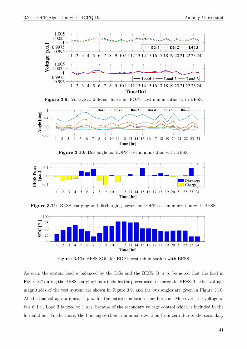
3.2. EOPF Algorithm with HCPQ Bus Aalborg Universitet
1 2 3 4 5 6 7 8 9 10 11 12 13 14 15 16 17 18 19 20 21 22 23 24
0.995
0.9975
1
1.0025
1.005
DG 1 DG 2 DG 3
1 2 3 4 5 6 7 8 9 10 11 12 13 14 15 16 17 18 19 20 21 22 23 24
Time [hr]
0.995
0.9975
1
1.0025
1.005
Volt
age
[p.u
.]
Load 1 Load 2 Load 3
Figure 3.9: Voltage at different buses for EOPF cost minimization with BESS.
1 2 3 4 5 6 7 8 9 10 11 12 13 14 15 16 17 18 19 20 21 22 23 24
Time [hr]
-0.5
0
0.5
1
An
gle
[d
eg] Bus 1 Bus 2 Bus 3 Bus 4 Bus 5 Bus 6
Figure 3.10: Bus angle for EOPF cost minimization with BESS.
1 2 3 4 5 6 7 8 9 10 11 12 13 14 15 16 17 18 19 20 21 22 23 24
Time [hr]
-0.1
0
0.1
BE
SS
Po
wer
[p.u
.]
Discharge
Charge
Figure 3.11: BESS charging and discharging power for EOPF cost minimization with BESS.
1 2 3 4 5 6 7 8 9 10 11 12 13 14 15 16 17 18 19 20 21 22 23 24
Time [hr]
0
25
50
75
100
SO
C [
%]
Figure 3.12: BESS SOC for EOPF cost minimization with BESS.
As seen, the system load is balanced by the DGs and the BESS. It is to be noted that the load in
Figure 3.7 during the BESS charging hours includes the power used to charge the BESS. The bus voltage
magnitudes of the test system are shown in Figure 3.9, and the bus angles are given in Figure 3.10.
All the bus voltages are near 1 p.u. for the entire simulation time horizon. Moreover, the voltage of
bus 6, i.e., Load 3 is fixed to 1 p.u. because of the secondary voltage control which is included in the
formulation. Furthermore, the bus angles show a minimal deviation from zero due to the secondary
41

3.2. EOPF Algorithm with HCPQ Bus Aalborg Universitet
frequency control included in the HCPQ formulation. The BESS charging-discharging power and SOC
are shown in Figure 3.11 and 3.12, respectively and it can be seen that the BESS operates within its
limits and the problem of simultaneous charging-discharging observed in 2.6 is also resolved.
3.2.4 Cost Minimization with Load Shedding
The optimization problem in (3.5) is revamped by changing the optimization objective to minimizing
cost due to load shedding and DG operation, with the presence of a storage device. This is done by
introducing a penalty factor VOLL for all the loads connected in the system, which is assumed to be
10 $/W . Thus, there is a trade-off between increasing the cost due to the load shedding penalty and
decreasing the operational cost from DGs. By including load shedding in the equation (3.5) the cost
optimization problem becomes as follows,
minKp
n Kqn ∆SOC(t) Pl
TH∑t=1
NG∑g=1
(agP2g (t) + bgPg(t) + cg) +
TH∑t=1
NL∑l=1
V OLL · Pl(t)
subject to, PBESS(t) + E ∆SOC(t) = 0
Pming − Pg(t) ≤ 0
Pg(t)− Pmaxg ≤ 0
Qming −Qg(t) ≤ 0
Qg(t)−Qmaxg ≤ 0
Kq minn −Kq
n ≤ 0
Kqn −Kq max
n ≤ 0
Kp minn −Kp
n ≤ 0
Kpn −Kp max
n ≤ 0
PBESS(d)
−E−∆SOC(t) ≤ 0
∆SOC(t)−PBESS(c)
−E≤ 0
SOC(t)− SOCmax ≤ 0
SOCmin − SOC(t) ≤ 0
Pl − PmaxLS ≤ 0
− Pl ≤ 0
(3.6)
Where PmaxLS is the maximum load shedding and it is assumed to be 10% of available load at time t
for all the loads connected in the system. The DG power limits and BESS limits are taken from 3.2.3.
42

3.2. EOPF Algorithm with HCPQ Bus Aalborg Universitet
The optimization problem was solved for t = 24 with the arbitrary load profiles shown in Figure 3.2.
The simulation took 99.68 min and 24 iterations. The cost was minimized to $ 6625.07. The inclusion
of load shedding to the test system reduces the operational cost by 0.06% compared to the base case
without BESS and load shedding. The droop coefficients after optimization are given in Table 3.6.
Table 3.6: Optimized droop coefficients for EOPF cost minimization with BESS and load shedding
Knp Kn
q
DG1 4.8636e-6 2.2470e-5DG2 3.9109e-5 4.9987e-4DG3 1.9553e-6 2.9970e-4
1 2 3 4 5 6 7 8 9 10 11 12 13 14 15 16 17 18 19 20 21 22 23 24
Time [hr]
-0.1
0
0.1
0.2
0.3
0.4
Act
ive
Pow
er [
p.u
.]
DG1 DG2 DG3 BESS Load shed1 Load shed2 Load shed3 Load
Figure 3.13: DG and BESS active power for EOPF cost minimization with BESS and loadshedding.
1 2 3 4 5 6 7 8 9 10 11 12 13 14 15 16 17 18 19 20 21 22 23 24
Time [hr]
0
0.05
0.1
0.15
Rea
ctiv
e P
ow
er
[p.u
.]
DG1 DG2 DG3 Load
Figure 3.14: DG reactive power for EOPF cost minimization with BESS and load shedding.
1 2 3 4 5 6 7 8 9 10 11 12 13 14 15 16 17 18 19 20 21 22 23 24
0.995
0.9975
1
1.0025
1.005
DG 1 DG 2 DG 3
1 2 3 4 5 6 7 8 9 10 11 12 13 14 15 16 17 18 19 20 21 22 23 24
Time [hr]
0.995
0.9975
1
1.0025
1.005
Vo
lta
ge
[p.u
.]
Load 1 Load 2 Load 3
Figure 3.15: Voltage at different buses for EOPF cost minimization with BESS and load shedding.
43

3.3. Summary Aalborg Universitet
1 2 3 4 5 6 7 8 9 10 11 12 13 14 15 16 17 18 19 20 21 22 23 24
Time [hr]
0
0.5
1
An
gle
[d
eg] Bus 1 Bus 2 Bus 3 Bus 4 Bus 5 Bus 6
Figure 3.16: Bus angles for EOPF cost minimization with BESS and load shedding.
1 2 3 4 5 6 7 8 9 10 11 12 13 14 15 16 17 18 19 20 21 22 23 24
Time [hr]
-0.1
-0.05
0
0.05
0.1
BE
SS
Po
wer
[p.u
.]
Discharge
Charge
Figure 3.17: BESS charging and discharging power for EOPF cost minimization with BESS andload shedding.
1 2 3 4 5 6 7 8 9 10 11 12 13 14 15 16 17 18 19 20 21 22 23 24
Time [hr]
0
25
50
75
100
SO
C [
%]
Figure 3.18: BESS SOC for EOPF cost minimization with BESS and load shedding.
The results for EOPF cost minimization with load shedding in the presence of BESS are shown in
Figure 3.13-3.18. Figure 3.13 shows the curtailment of load for t=24 to minimize the cost, while the
reactive power is shown in Figure 3.14. In Figure 3.13, the sum of the DG power, the load shed and
BESS contribution amount to the total available load in the system at that hour. The bus voltage
magnitudes are near to 1 p.u. for the given test system as shown in Figure 3.15 and the bus angles
are close to zero and illustrated in Figure 3.16. The BESS charging-discharging power and SOC are
shown in Figure 3.17 and 3.18 and it can be seen that the BESS operates within its limits.
3.3 Summary
In this chapter, the extended optimal power flow algorithm with HCPQ bus is presented and tested
for various cases. The proposed hierarchical scheme includes a tertiary level control to meet various
optimization objectives such as equal active power and reactive power sharing, cost minimization with
BESS, and cost minimization with load shedding. The results obtained from the case studies indicate
that the application of the proposed hierarchically control EOPF scheme contribute to an optimized
and reliable operation of the microgrid.
44

3.3. Summary Aalborg Universitet
Table 3.7: Summary of results for EOPF cost minimization.
Case Time [min] Iterations Cost [$]Base 5.95 16 6629.38
With BESS 34.94 38 6628.50With LoadShedding 99.68 24 6625.07
A Summary of the cost minimization results are given in Table 3.7. The inclusion of a BESS to the
EOPF problem increases the complexity of the problem, however, it may help in reducing the cost of
the system if at least one of the DG units has a very low or zero operating cost, such as RES. The
cost associated with RES is usually for curtailment rather than operation. Hence, the inclusion of a
BESS in a system with RES would reduce the system cost by charging from the RES power, reducing
RES curtailment, and then discharging to reduce the power contribution from the costly DGs. The
inclusion of load shedding further increases the complexity, but the cost can be decreased. For load
shedding to be effective, the cost of shedding the load, i.e., VOLL should be comparatively much less
than the cost of operating DGs. In general, load shedding is feasible when the load demand is larger
than the available power generation.
To further validate the proposed hierarchical scheme, the algorithm will be tested on a CIGRE
benchmark system in the following chapters.
45

4 | CIGRE Microgrid: Power Flow
4.1 Introduction
In this chapter, the steady-state power flow analysis is carried out for a modified CIGRE benchmark
microgrid with a 12.47 kV MV distribution network [35, 36, 37]. Initially, the steady-state analysis
using the conventional power flow is performed. Later, from the results of this study, selection of
buses for the hierarchical extended power flow analysis is done, in order to maintain the bus voltage
magnitudes and system frequency at their desirable values.
4.2 CIGRE Microgrid Topology
The single line diagram of the modified CIGRE benchmark network is shown in Figure 4.1. There is no
connection to the main grid, hence the microgrid is islanded. It has Solar Photo-Voltaic (SPV) panels,
WTs, CG units and BESS as DERs. The line parameters for the system are given in the Table B.1
in Appendix B. The transformer parameters (480 V/12.47 kV) connected between bus 14 and 1 are
taken from [35] and are given in Table B.2 in Appendix B.
The loads that are included in the network are aggregated loads and are separated as industrial and
household loads as shown in the Table B.3 in Appendix B. Each industrial and household load follows
the same load patterns respectively with different load scaling based on the power consumption by the
consumers. The hourly industrial and household load profile is shown in Figure B.1 in Appendix B.
The total generation capacity in the modified CIGRE benchmark system in [35, 37] is much higher
than the load. Hence, the grid was further modified by removing the 2500 kW and 800 kW units
from bus 14. The microgrid now has a total DG capacity of 4290 kW and a BESS of capacity 1000
kWh, with its parameters given in Table B.5 in Appendix B. DER with different capacity connected
to each bus are listed in the Table B.4 in Appendix B. The typical hourly normalized wind and solar
PV output profiles are taken from [37] and are shown in Figure B.2 in Appendix B. The voltage limits
are considered as +5% and -10% of the nominal value as per IEC 60038 [38] and from EN 50160 [39],
and the frequency limits of ±1% of nominal frequency are considered for the power flow analysis of
the MV modified CIGRE microgrid.
46

4.3. Power Flow Case Study Aalborg Universitet
14
1
2
3
4
11
12
13
5
~||
10
9
8
480 V
12.47 kV
7
x3
6
~||
~||
~||
~||
~||
~||
~||
~||
Figure 4.1: Modified CIGRE benchmark network.
4.3 Power Flow Case Study
To improve the steady state behaviour of the modified CIGRE microgrid benchmark, it is imperative
to first perform a power flow analysis before deciding which processes to optimize. For this purpose,
a power flow based case study is performed in this chapter. The inferences from this study would act
as a reference when discussing the results in the EOPF-based case study in chapter 5.
Two power flow based case studies are considered in this chapter, which differ in their methodology.
In the first case, a conventional power flow study is performed on the modified CIGRE benchmark
microgrid. This is done in order to examine the behaviour of the system assuming it as a conventional
power system network. The results of this study are used to determine which buses need to be controlled
47

4.4. Simulation Results Aalborg Universitet
using the HCPQ bus formulation described in 2.5.1.2. This directly leads to the next case, which is
based on HC of microgrid power flow using the HCPQ bus method. The results from this case would
be more accurate as they would better represent the dynamics of the microgrid and its components,
and also address some of the assumptions made in the conventional power flow case. Finally, the
shortcoming of this case would be identified and addressed in the next chapter, which includes an
EOPF-based case study. The power flow based cases are described in detail below. The tolerance for
NR was set to 10−6.
1. Case 0: Conventional Power Flow
• Bus 14 is considered as slack bus.
• Buses 1-13 are considered as PQ buses.
• BESS is neglected.
• The RES generate based on their hourly profile. The CGs generate at a fixed capacity.
The DGs, RES and CGs, in the system are considered to have the same percentage of
maximum capacity. Consequently, two sub-cases are simulated with the following percentage
of maximum available capacity:
– 100%– 50%
• Based on the bus voltage magnitudes observed in this case, the buses which exceed the
voltage limit will be controlled in the next case.
2. Case 1: HC Power Flow
• Bus 14 is considered as PV bus.
• Buses 1, 2, 12 and 13 are considered as PQ buses.
• Based on the results from case 0, buses 3-11 are either HCPQ buses or PQ buses.
• BESS is neglected.
• The CGs in the system are considered to generate the same percentage of maximum capacity.
The share is chosen based on the results of case 0.
• Droop coefficients are estimated using the droop equations (2.1) and (2.2).
• Based on the results obtained, the constraints and optimization variables for the
optimization level would be decided.
4.4 Simulation Results
The two cases described in 4.3 were simulated in MATLAB and the results are described below. The
total system load capacity is 0.4425 p.u. for active load, and 0.0841 p.u. for reactive load, based on
the data given in Table B.3 in Appendix B. The system base value was chosen as 1000 kVA. Since the
48

4.4. Simulation Results Aalborg Universitet
total DG capacity is 4290 kW, the load was increased by a factor of 3. The power factor was taken as
0.8, which is used to calculate the reactive power capacities of the DG units.
4.4.1 Case 0: Conventional Power Flow
The results of the simulation for the model in Figure 4.1 with 100% DG capacity are illustrated in
Figure 4.2 - 4.4. From Figure 4.2, it can be seen that the voltage magnitude exceeds the +5% limit
for buses 3-11 during t = 10 to t = 21.
It should be noted that these buses are the the buses with RES. The bus angles deviate by less than
a couple degrees from zero, as seen from Figure 4.3.
1 2 3 4 5 6 7 8 9 10 11 12 13 14 15 16 17 18 19 20 21 22 23 24
Time [hr]
0.975
1
1.025
1.05
1.075
1.1
Volt
age
[p.u
.]
Bus 1 Bus 2 Bus 3 Bus 4 Bus 5 Bus 6 Bus 7
(a) Bus 1-7
1 2 3 4 5 6 7 8 9 10 11 12 13 14 15 16 17 18 19 20 21 22 23 24
Time [hr]
0.975
1
1.025
1.05
1.075
1.1
Vo
lta
ge
[p.u
.]
Bus 8 Bus 9 Bus 10 Bus 11 Bus 12 Bus 13 Bus 14
(b) Bus 8-14
Figure 4.2: Bus voltage magnitude for case 0 with 100% DG capacity.
1 2 3 4 5 6 7 8 9 10 11 12 13 14 15 16 17 18 19 20 21 22 23 24
Time [hr]
-0.25
0
0.25
0.5
0.75
1
An
gle
[d
eg]
Bus 1 Bus 2 Bus 3 Bus 4 Bus 5 Bus 6 Bus 7
(a) Bus 1-7
1 2 3 4 5 6 7 8 9 10 11 12 13 14 15 16 17 18 19 20 21 22 23 24
Time [hr]
-0.25
0
0.25
0.5
0.75
1
An
gle
[d
eg]
Bus 1 Bus 2 Bus 3 Bus 4 Bus 5 Bus 6 Bus 7
(b) Bus 8-14
Figure 4.3: Bus angles for case 0 with 100% DG capacity.
49

4.4. Simulation Results Aalborg Universitet
1 2 3 4 5 6 7 8 9 10 11 12 13 14 15 16 17 18 19 20 21 22 23 24
Time [hr]
-2000
-1000
0
1000
2000
3000
Acti
ve P
ow
er [
kW
] CG Slack RES Load Loss
(a) Active Power
1 2 3 4 5 6 7 8 9 10 11 12 13 14 15 16 17 18 19 20 21 22 23 24
Time [hr]
-2000
-1000
0
1000
2000
Reacti
ve P
ow
er [
kV
AR
]
CG Slack RES Load Loss
(b) Reactive Power
Figure 4.4: Power balance for case 0 with 100% DG capacity.
In Figure 4.4, it is noticed that since the CGs and RES generate to their maximum capacity, the slack
needs to absorb the excess active and reactive power in order to bring the system in balance. To
observe the change in this behaviour, the DG capacity needs to be reduced. Hence the other sub-case
with 50% capacities becomes relevant to the study. The results for 50% case are given in Figure 4.5,
4.6 and in Figure C.1 in Appendix C. Figure 4.5 indicates that the maximum voltage magnitude for
buses 3-11 drops down to +3% on reducing the DG capacities.
1 2 3 4 5 6 7 8 9 10 11 12 13 14 15 16 17 18 19 20 21 22 23 24
Time [hr]
0.975
1
1.025
1.05
Volt
age
[p.u
.]
Bus 1 Bus 2 Bus 3 Bus 4 Bus 5 Bus 6 Bus 7
(a) Bus 1-7
1 2 3 4 5 6 7 8 9 10 11 12 13 14 15 16 17 18 19 20 21 22 23 24
Time [hr]
0.975
1
1.025
1.05
Volt
age
[p.u
.]
Bus 8 Bus 9 Bus 10 Bus 11 Bus 12 Bus 13 Bus 14
(b) Bus 8-14
Figure 4.5: Bus voltage magnitude for case 0 with 50% DG capacity.
50

4.4. Simulation Results Aalborg Universitet
The bus angle in Figure C.1 shows no change that could be of any significance to the study. The
decrease in DG capacity shows an improvement in active power balance in Figure 4.6., but only for
some hours. Since there is no curtailment of RES power, the slack bus is required to absorb the excess
power. The reactive power behaviour, however, does not change.
1 2 3 4 5 6 7 8 9 10 11 12 13 14 15 16 17 18 19 20 21 22 23 24
Time [hr]
-500
0
500
1000
1500
Acti
ve P
ow
er [
kW
] CG Slack RES Load Loss
(a) Active Power
1 2 3 4 5 6 7 8 9 10 11 12 13 14 15 16 17 18 19 20 21 22 23 24
Time [hr]
-1000
-500
0
500
1000
Reacti
ve P
ow
er [
kV
AR
]
CG Slack RES Load Loss
(b) Reactive Power
Figure 4.6: Power balance for case 0 with 50% DG capacity.
Each sub-case took 4-5 iterations for each hour and the total system losses are given in Table 4.1. The
convergence error at each hour was in the order of 10−7 or smaller. The losses in the system decrease
significantly with the decrease in DG capacity, although they are still quite high. This suggests that
the system generation needs to be better managed. In the next case, the percentage share of each
CGs is taken as 10%. It may be, however, noted that the only CG present in the system in case 0
are on bus 9 and 13 of capacity 300 kW each, since bus 14 is considered as a slack bus. Finally, it
may be concluded that buses 3-11 are needed to be controlled as HCPQ buses in order to reduce RES
generation output and maintain the bus voltage magnitude within the admissible limits, as close to 1
p.u as possible. Moreover, bus 14 cannot be a slack bus since it has a limited capacity. Furthermore,
it can only generate active power and not absorb it, contrary to what the results with active power
balance suggest. Hence it should be made a PV bus.
51

4.4. Simulation Results Aalborg Universitet
Table 4.1: Active and reactive power system loss for case 0.
DG Capacity Active Power Loss [kW] Reactive Power Loss [kVAR]100% 1490.29 1664.5150% 376.71 348.70
% change 295.61 377.34
4.4.2 Case 1: Controlled Power Flow
After analyzing the simulation results from case 0, case 1 was simulated in MATLAB. Each hour
took 2-3 iterations to converge with a convergence error of 10−7 or smaller. Buses 3-11 were taken
as references to control the voltage on their respective bus. Bus 1 was taken as the reference bus for
secondary frequency control. The secondary frequency control parameter kiw was taken as 4, as given in
Table B.1, and the droop coefficients were as given in Table C.1 in Appendix C. These droop coefficients
are calculated based on the droop equations by using the reference frequency, reference voltage and
RES active and reactive power capacities, to get the droop coefficients kp and kq respectively. To
estimate an accurate set of droop coefficients, they need to be included to the set of optimization
variables.
1 2 3 4 5 6 7 8 9 10 11 12 13 14 15 16 17 18 19 20 21 22 23 24
Time [hr]
0.98
0.99
1
1.01
1.02
Vo
lta
ge
[p.u
.]
Bus 1 Bus 2 Bus 3 Bus 4 Bus 5 Bus 6 Bus 7
(a) Bus 1-7
1 2 3 4 5 6 7 8 9 10 11 12 13 14 15 16 17 18 19 20 21 22 23 24
Time [hr]
0.98
0.99
1
1.01
1.02
Volt
age
[p.u
.]
Bus 8 Bus 9 Bus 10 Bus 11 Bus 12 Bus 13 Bus 14
(b) Bus 8-14
Figure 4.7: Bus voltage magnitude for case 1 with 10% CG capacity.
The bus voltage was controlled to stay within the limits. In fact, since the reference voltage for HCPQ
buses was taken as 1 p.u., buses 3-11 had 1 p.u. voltage throughout the time horizon. This can be
seen from Figure 4.7. Figure 4.8 indicates that the bus angles have a small phase shift, but are close
to 0 deg.
Figure 4.9 shows the system hourly power balance with 10% CG capacity. While the active power
is properly balanced, the problem of excess reactive power still persists. This is due to the fact that
52

4.4. Simulation Results Aalborg Universitet
1 2 3 4 5 6 7 8 9 10 11 12 13 14 15 16 17 18 19 20 21 22 23 24
Time [hr]
0
0.5
1
An
gle
[d
eg]
Bus 1 Bus 2 Bus 3 Bus 4 Bus 5 Bus 6 Bus 7
(a) Bus 1-7
1 2 3 4 5 6 7 8 9 10 11 12 13 14 15 16 17 18 19 20 21 22 23 24
Time [hr]
-0.5
0
0.5
1
An
gle
[d
eg]
Bus 8 Bus 9 Bus 10 Bus 11 Bus 12 Bus 13 Bus 14
(b) Bus 8-14
Figure 4.8: Bus angles for case 1 with 10% CG capacity.
1 2 3 4 5 6 7 8 9 10 11 12 13 14 15 16 17 18 19 20 21 22 23 24
Time [hr]
0
200
400
600
800
1000
Acti
ve P
ow
er [
kW
]
CG RES Load Loss
(a) Active Power
1 2 3 4 5 6 7 8 9 10 11 12 13 14 15 16 17 18 19 20 21 22 23 24
Time [hr]
-500
0
500
1000
Rea
cti
ve P
ow
er [
kV
AR
]
CG RES Load Loss
(b) Reactive Power
Figure 4.9: Power balance for case 1 with 10% CG capacity.
the PV bus (bus 14) is required to be maintained at 1 p.u. Therefore, the CG on bus 14 generates
reactive power to maintain that voltage level and consequently there is an excess of reactive power in
the system. This power is absorbed by the HCPQ buses connected to RES, which themselves are also
required to maintain 1 p.u. at their buses. In order to reduce the reactive power contribution by the
CG at bus 14, the PV bus voltage needs to be reduced. In the following scenario, the PV bus voltage
is reduced to 0.995 p.u.
53

4.4. Simulation Results Aalborg Universitet
4.4.2.1 Decrease in PV Bus Voltage
On decreasing the PV bus voltage to 0.995 p.u., as shown in Figure 4.10, the reactive power contribution
from the CG on bus 14 decreases. This is illustrated in Figure 4.11. The bus angles and active power
balance are given in Figure C.2 and C.3 in Appendix C. However, there is still an issue of excess reactive
power. It is observed that during the day time, the CG gives excessive reactive power, whereas during
the night the RES give excess reactive power. In order to further improve the reactive power balance,
the voltage at the HCPQ buses can be increased.
1 2 3 4 5 6 7 8 9 10 11 12 13 14 15 16 17 18 19 20 21 22 23 24
Time [hr]
0.98
0.99
1
1.01
1.02
Volt
age
[p.u
.]
Bus 1 Bus 2 Bus 3 Bus 4 Bus 5 Bus 6 Bus 7
(a) Bus 1-7
1 2 3 4 5 6 7 8 9 10 11 12 13 14 15 16 17 18 19 20 21 22 23 24
Time [hr]
0.98
0.99
1
1.01
1.02
Vo
lta
ge
[p.u
.]
Bus 8 Bus 9 Bus 10 Bus 11 Bus 12 Bus 13 Bus 14
(b) Bus 8-14
Figure 4.10: Bus voltage magnitude for case 1 with PV bus voltage 0.995 p.u.
1 2 3 4 5 6 7 8 9 10 11 12 13 14 15 16 17 18 19 20 21 22 23 24
Time [hr]
-400
-200
0
200
400
600
Reacti
ve P
ow
er [
kV
AR
]
CG RES Load Loss
Figure 4.11: Reactive power balance for case 1 with PV bus voltage 0.995 p.u.
4.4.2.2 Increase in HCPQ Bus Voltage
Due to the effect of the droop control dynamics, the voltage-reactive power relation is inverse for HCPQ
buses. In order to reduce the reactive power contribution from the HCPQ buses, their reference voltage
must be increased. In this scenario, the HCPQ reference voltage is increased to 1.005 p.u, as shown in
Figure 4.12. The bus angles and active power balance are given in Figure C.4 and C.5 in Appendix C.
The reactive power is balanced for more than half of the time horizon, as given in Figure 4.13. Table 4.2
54

4.4. Simulation Results Aalborg Universitet
compares the system loss for the three scenarios discussed in case 1 simulations. A notable change in
reactive power loss is observed on changing the reference voltages. Finally, it may be concluded that
the varying voltage references are needed for the PV and HCPQ buses throughout the time horizon in
order to observe proper reactive balance.
1 2 3 4 5 6 7 8 9 10 11 12 13 14 15 16 17 18 19 20 21 22 23 24
Time [hr]
0.98
0.99
1
1.01
1.02
Vo
lta
ge
[p.u
.]
Bus 1 Bus 2 Bus 3 Bus 4 Bus 5 Bus 6 Bus 7
(a) Bus 1-7
1 2 3 4 5 6 7 8 9 10 11 12 13 14 15 16 17 18 19 20 21 22 23 24
Time [hr]
0.98
0.99
1
1.01
1.02
Volt
age
[p.u
.]
Bus 8 Bus 9 Bus 10 Bus 11 Bus 12 Bus 13 Bus 14
(b) Bus 8-14
Figure 4.12: Bus voltage magnitude for case 1 with PV bus voltage 0.995 p.u. and HCPQ busvoltage 1.005 p.u.
1 2 3 4 5 6 7 8 9 10 11 12 13 14 15 16 17 18 19 20 21 22 23 24
Time [hr]
-400
-200
0
200
400
600
Rea
cti
ve P
ow
er [
kV
AR
]
CG RES Load Loss
Figure 4.13: Reactive power balance for case 1 with PV bus voltage 0.995 p.u. and HCPQ busvoltage 1.005 p.u.
Table 4.2: Active and reactive power system loss for case 1.
PV BusVoltage [p.u.]
HCPQ BusVoltage [p.u.]
Active PowerLoss [kW]
Reactive PowerLoss [kVAR]
1 1 260.40 233.800.995 1 233.38 163.730.995 1.005 230.64 163.03
In order to effectively utilize the RES generation, a BESS is needed in the system. Secondly, the
generation capacities of the CGs need to be taken into account, along with the maximum and minimum
generation limits of all DGs. Furthermore, it may also be asserted to put soft voltage limits on the
55

4.5. Summary Aalborg Universitet
HCPQ bus and PV bus. This would allow more flexibility in the system by not burdening the DGs
to provide the required amount of reactive power in order to maintain 1 p.u. bus voltage. Finally, an
appropriate selection of droop coefficients is also required. These constraints can be included in the
tertiary level of control, i.e., the optimization level.
4.5 Summary
This chapter discussed the topology of a modified MV CIGRE benchmark microgrid that is used
in this study. The system is examined by initially performing a conventional power flow analysis.
However, that requires certain assumptions such as the need of a slack bus, a fixed system frequency,
and pre-defined active and reactive powers of the DGs. Based on the outcomes, a controlled microgrid
power flow study is performed which also addresses the aforementioned assumptions of the conventional
study. Nevertheless, the controlled power flow is also not completely robust and requires a higher level
of optimization so as to take certain system and component constraints into account. For this purpose,
this study is extended in the next chapter to investigate EOPF in the CIGRE network.
56

5 | CIGRE Microgrid: EOPF
5.1 Introduction
Based on the results and conclusions drawn from 4.4.2, there is a need for a tertiary control level
to optimize system operation while ensuring the system components operate within their operational
limits. The study of the MV CIGRE benchmark microgrid illustrated in Figure 4.1 is, therefore,
extended to include optimization, along with the hierarchically-controlled power flow. Hence, in this
chapter, the EOPF analysis is implemented for the modified CIGRE benchmark network. To facilitate
this, the control algorithm for EOPF described in Figure 3.1 in 3.2 is explored for different optimization
objectives which are stated below,
1. Case 2: Minimizing the operational cost of CGs and RES curtailment.
2. Case 3: Minimizing the operational cost of CGs with the inclusion of load shedding constraints.
5.2 Case 2: Renewable Power Curtailment
The increased penetration of RES into the distribution network minimizes the contribution of CGs to
supply the required demand and reduces environmental emissions. However, when RES penetration
is more than the actual demand in the system it causes many problems such as excessive line losses,
overloading of transformers and feeders, protection failure, over-voltage issues, etc [40]. Hence, there
is a need for RES curtailment. This is achieved by introducing a penalty factor for RES curtailed
power, which is assumed as 50$/MW throughout this study. The cost coefficients for the CGs were
taken from [35, 37] and are also given in Table B.6 in Appendix B. The inclusion of RES curtailment
in the optimization objective is expected to complement the minimization of CG operational cost, and
increase the RES utilization. Moreover, the presence of BESS in the system would further aid the
objective by managing the excess, or deficit, RES power and in turn, reduce the overall operating cost
in the system.
Based on the inferences from the power flow analysis in chapter 4, the following changes are made to
the optimization formulation, in order to incorporate the EOPF algorithm. Firstly, voltage soft limits
are included for PV and HCPQ buses. The reason for this is to allow for flexibility in the system, so
that the DGs are not required to maintain exactly 1 p.u. on their respective buses. The reference power
for all the CGs is calculated in the optimization, and then given to the controlled power flow layer.
57

5.2. Case 2: Renewable Power Curtailment Aalborg Universitet
The minimum reactive power that can be generated by a given DG for reactive power compensation
is decided by the unit operator and is assumed to be zero for simplicity in this study. The boundaries
for the droop coefficients are assumed as follows,
2× 10⁻⁷ ≤ Kpn ≤ 5× 10⁻⁴ (5.1) 2× 10⁻⁶ ≤ Kp
n ≤ 5× 10⁻³ (5.2)
The most prominent change is in the functioning of the HCPQ buses with SPV, i.e., all HCPQ buses
except bus 7, during different durations of the time horizon. The time horizon can be broadly broken
down into two categories described below, which can also be seen in Figure B.2 in Appendix B
• Night phase: t=1 to t=6, and t=22 to t=24
• Day phase: t=7 to t=21
The optimization requires the HCPQ buses to generate within the upper and lower bounds. The lower
bound is fixed to zero, as mentioned earlier, and the upper bound is based on the DG capacity and
power profile. During the night phase there is zero solar power. Hence, the optimization would require
the solar HCPQ buses to generate exactly zero active and reactive power. However, as per the HCPQ
bus active power equation (2.19) , which is also given below, for power to be zero, either δm = δ0m
or Kpn should be extremely large. Similarly as per the reactive power equation from (2.20), either
|V ∗n | − |Vn|+ U intv = 0 or Kq
n should be extremely large.
P (scheduled)n =
−Kiw(δm − δ0m)
Kpn
Q(scheduled)n =
|V ∗n | − |Vn|+ U intv
Kqn
Either of these are not feasible. The droop coefficients have an upper limit, and the bus angle cannot
be made exactly equal to its reference value, given the presence of loads also on those buses. If the bus
voltage is fixed to its reference value, only the secondary voltage integral parameter U intv and droop
coefficient Kqn affect the scheduled reactive power of the bus. Dividing these two parameters cannot
give a value which would satisfy the optimization constraint tolerance. Hence, to solve this issue, the
solar HCPQ buses were made as PQ buses during the night phase with P and Q set to zero.
To investigate the system behaviour, different scenarios for RES curtailment are considered in this
section, as given below,
1. Change in voltage soft limits for PV and HCPQ buses.
2. Change in DG power factor.
3. Presence of non-linear load.
In all scenarios, the optimization variables are
58

5.2. Case 2: Renewable Power Curtailment Aalborg Universitet
• the droop coefficients,
• hourly change in BESS SOC (The initial SOC is assumed to be 50%.),
• hourly active and reactive power references of CGs on HCPQ bus 9 and PQ bus 13,
• hourly active power references for CG on PV bus 14,
• and voltage soft limits for PV and HCPQ buses.
The optimization problem is thus formulated as follows,
minx
TH∑t=1
NG∑g=1
(agP2g (t) + bgPg(t) + cg) +
TH∑t=1
NRES∑N=1
CRES · PRES(t)
where, x = Kpn, K
qn, ∆SOC(t), PCG, QCG, VPV and VHCPQ
subject to, PBESS(t) + E ·∆SOC(t) = 0
Pming, RES − Pg, RES(t) ≤ 0
Pg, RES(t)− Pmaxg, RES ≤ 0
Qming, RES −Qg, RES(t) ≤ 0
Qg, RES(t)−Qmaxg, RES ≤ 0
Kq minn −Kq
n ≤ 0
Kqn −Kq max
n ≤ 0
Kp minn −Kp
n ≤ 0
Kpn −Kp max
n ≤ 0
PBESS(d)
−E−∆SOC(t) ≤ 0
∆SOC(t)−PBESS(c)
−E≤ 0
SOC(t)− SOCmax ≤ 0
SOCmin − SOC(t) ≤ 0
VPV, HCPQ − V maxPV, HCPQ ≤ 0
V minPV, HCPQ − VPV, HCPQ ≤ 0
(5.3)
The simulations were performed in MATLAB using fmincon function with SQP algorithm. As per
MATLAB documentation, the SQP algorithm, is much faster than the default interior-point algorithm
and takes a lesser number of iterations, comparatively. The MATLAB code for this case is given in
Appendix F. Comments in the code have also been provided for the reader’s understanding. The same
code can also be used for the different scenarios or the Load Shedding case with minor modifications.
59

5.2. Case 2: Renewable Power Curtailment Aalborg Universitet
5.2.1 Voltage Soft Limit
In this section, cost minimization with RES curtailment is performed with two different voltage soft
limits for both PV and HCPQ buses, namely, ±1% and ±2% p.u. soft limits. These voltage variables
are included in the optimization level. These voltage variables are then used as references for the
respective buses in the hierarchically controlled power flow level. The simulations took 16.08 and 7.63
hours with 36 and 14 iterations respectively, for the two scenarios. The cost obtained in two scenarios
was equal to $ 682575.29 and $ 682150.38, respectively. The various results for the two scenarios are
illustrated in Figure 5.1-5.6.
1 2 3 4 5 6 7 8 9 10 11 12 13 14 15 16 17 18 19 20 21 22 23 24
Time [hr]
0.97
0.98
0.99
1
1.01
1.02
Vo
lta
ge
[p.u
.] Bus 1 Bus 2 Bus 3 Bus 4 Bus 5 Bus 6 Bus 7
(a) Bus 1-7
1 2 3 4 5 6 7 8 9 10 11 12 13 14 15 16 17 18 19 20 21 22 23 24
Time [hr]
0.97
0.98
0.99
1
1.01
1.02
Vo
lta
ge
[p.u
.] Bus 8 Bus 9 Bus 10 Bus 11 Bus 12 Bus 13 Bus 14
(b) Bus 8-14
Figure 5.1: Bus voltage magnitude for case 2 with 1% voltage soft limits.
As observed from Figure 5.1, the ±1% soft voltage limit facilitates the voltage for HCPQ buses 3-11 to
be above 1 p.u. during the day hours, thereby effecting the reactive power contribution of the HCPQ
buses. Only buses 1, 12 and 13 fall slightly below the 1% voltage limit but that is because those are
PQ buses. In comparison for ±2% soft limits in Figure 5.2, the HCPQ bus voltage drops below 1 p.u.
during the day hours causing the RES reactive power contribution to be more in contrast to the ±1%
soft limit scenario. This is also evident from Figure 5.3 and 5.4 which show the active and reactive
power balance for the two scenarios.
In both scenarios, there is no contribution from the CGs towards the active power balance, which is in
order with the optimization objectives of minimization of CG operational cost and RES curtailment.
The utilized and available hourly RES active power for both scenarios is displayed in Figure 5.5 and
60

5.2. Case 2: Renewable Power Curtailment Aalborg Universitet
1 2 3 4 5 6 7 8 9 10 11 12 13 14 15 16 17 18 19 20 21 22 23 24
Time [hr]
0.97
0.98
0.99
1
1.01
1.02 V
olt
ag
e [p
.u.] Bus 1 Bus 2 Bus 3 Bus 4 Bus 5 Bus 6 Bus 7
(a) Bus 1-7
1 2 3 4 5 6 7 8 9 10 11 12 13 14 15 16 17 18 19 20 21 22 23 24
Time [hr]
0.97
0.98
0.99
1
1.01
1.02
Vo
lta
ge
[p.u
.] Bus 8 Bus 9 Bus 10 Bus 11 Bus 12 Bus 13 Bus 14
(b) Bus 8-14
Figure 5.2: Bus voltage magnitude for case 2 with 2% voltage soft limits.
1 2 3 4 5 6 7 8 9 10 11 12 13 14 15 16 17 18 19 20 21 22 23 24
Time [hr]
0
500
1000
Act
ive
Po
wer
[k
W] CG RES Discharge
Load Loss Charge
(a) Active Power
1 2 3 4 5 6 7 8 9 10 11 12 13 14 15 16 17 18 19 20 21 22 23 24
Time [hr]
0
50
100
150
200
250
Reacti
ve P
ow
er [
kV
AR
]
CG RES Load Loss
(b) Reactive Power
Figure 5.3: Power balance for case 2 with 1% voltage soft limits.
5.6. In ±1% limit scenario, 55.98% of the RES power is utilized, whereas in the other scenario 56.01%
is used. The change in voltage soft limit has a marginal affect on the RES utilization. The BESS,
on the other hand, certainly assists in the optimization objective by managing the excess RES active
61

5.2. Case 2: Renewable Power Curtailment Aalborg Universitet
1 2 3 4 5 6 7 8 9 10 11 12 13 14 15 16 17 18 19 20 21 22 23 24
Time [hr]
0
500
1000
1500
Act
ive
Po
wer
[k
W]
CG RES Discharge Load Loss Charge
(a) Active Power
1 2 3 4 5 6 7 8 9 10 11 12 13 14 15 16 17 18 19 20 21 22 23 24
Time [hr]
0
50
100
150
200
250
Reacti
ve P
ow
er [
kV
AR
]
CG RES Load Loss
(b) Reactive Power
Figure 5.4: Power balance for case 2 with 2% voltage soft limits.
1 2 3 4 5 6 7 8 9 10 11 12 13 14 15 16 17 18 19 20 21 22 23 24
Time [hr]
0
500
1000
1500
2000
RE
S P
ow
er [
kW
]
Available
Used
Figure 5.5: RES curtailment for case 2 with 1% voltage soft limits.
1 2 3 4 5 6 7 8 9 10 11 12 13 14 15 16 17 18 19 20 21 22 23 24
Time [hr]
0
500
1000
1500
2000
RE
S P
ow
er [
kW
]
Available
Used
Figure 5.6: RES curtailment for case 2 with 2% voltage soft limits.
power, which is also evident from the power balance results. The BESS charging and discharging
power, and SOC are given in Figure 5.7 and 5.8.
Finally, the bus angles are shown in Figure 5.9 and 5.10, and as seen there is very little phase shift in
the bus angles.
62

5.2. Case 2: Renewable Power Curtailment Aalborg Universitet
2 4 6 8 10 12 14 16 18 20 22 24
Time [hr]
0
20
40
60
80
100
SO
C [
%]
(a) SOC
2 4 6 8 10 12 14 16 18 20 22 24
Time [hr]
-0.5
-0.25
0
0.25
0.5
Po
wer
[p
.u.]
Discharge
Charge
(b) BESS Power
Figure 5.7: BESS usage for case 2 with 1% voltage soft limits.
2 4 6 8 10 12 14 16 18 20 22 24
Time [hr]
0
20
40
60
80
100
SO
C [
%]
(a) SOC
2 4 6 8 10 12 14 16 18 20 22 24
Time [hr]
-0.5
-0.25
0
0.25
0.5
Po
wer
[p
.u.]
Discharge Charge
(b) BESS Power
Figure 5.8: BESS usage for case 2 with 2% voltage soft limits.
1 2 3 4 5 6 7 8 9 10 11 12 13 14 15 16 17 18 19 20 21 22 23 24
Time [hr]
0
0.2
0.4
0.6
An
gle
[d
eg]
Bus 1 Bus 2 Bus 3 Bus 4 Bus 5 Bus 6 Bus 7
(a) Bus 1-7
1 2 3 4 5 6 7 8 9 10 11 12 13 14 15 16 17 18 19 20 21 22 23 24
Time [hr]
-0.5
0
0.5
An
gle
[d
eg]
Bus 8 Bus 9 Bus 10 Bus 11 Bus 12 Bus 13 Bus 14
(b) Bus 8-14
Figure 5.9: Bus angle for case 2 with 1% voltage soft limits.
63

5.2. Case 2: Renewable Power Curtailment Aalborg Universitet
1 2 3 4 5 6 7 8 9 10 11 12 13 14 15 16 17 18 19 20 21 22 23 24
Time [hr]
0
0.2
0.4
0.6
An
gle
[d
eg]
Bus 1 Bus 2 Bus 3 Bus 4 Bus 5 Bus 6 Bus 7
(a) Bus 1-7
1 2 3 4 5 6 7 8 9 10 11 12 13 14 15 16 17 18 19 20 21 22 23 24
Time [hr]
-0.5
0
0.5
An
gle
[d
eg]
Bus 8 Bus 9 Bus 10 Bus 11 Bus 12 Bus 13 Bus 14
(b) Bus 8-14
Figure 5.10: Bus angle for case 2 with 2% voltage soft limits.
5.2.2 DG Power Factor
In this scenario to investigate the system behaviour for change in power factor is analyzed. The CG
cost minimization with RES curtailment is performed by changing the DG power factor from 0.8 to
0.9 and the voltage soft limits of PV and HCPQ buses is ±1%. The simulation optimized to a cost of
$ 682324.43 and it took 7.4 hours with 16 iterations.
1 2 3 4 5 6 7 8 9 10 11 12 13 14 15 16 17 18 19 20 21 22 23 24
Time [hr]
0.98
0.99
1
1.01
1.02
Vo
lta
ge
[p.u
.] Bus 1 Bus 2 Bus 3 Bus 4 Bus 5 Bus 6 Bus 7
(a) Bus 1-7
1 2 3 4 5 6 7 8 9 10 11 12 13 14 15 16 17 18 19 20 21 22 23 24
Time [hr]
0.98
0.99
1
1.01
1.02
Vo
lta
ge
[p.u
.] Bus 8 Bus 9 Bus 10 Bus 11 Bus 12 Bus 13 Bus 14
(b) Bus 8-14
Figure 5.11: Bus voltage magnitude for case 2 with 0.9 DG power factor.
64

5.2. Case 2: Renewable Power Curtailment Aalborg Universitet
The various results of the simulation are shown in Figure 5.11-D.2. As observed from Figure 5.11, the
voltage for HCPQ buses 3-11 lies between ±1% limit of nominal voltage and the voltage for PQ buses
1, 12 and 13 falls slightly below the 1% voltage limit.
From Figure 5.12 it is observed that the reactive power contribution from RES increases in comparison
with Figure 5.3, to ensure the voltage at HCPQ bus is between ±1% voltage soft limits. Since the DG
power factor has increased, the reactive power capacities, and hence reactive generation by the CGs
also decreases. Therefore, to compensate this decrease and balance the load, the RES are required to
give more reactive power.
1 2 3 4 5 6 7 8 9 10 11 12 13 14 15 16 17 18 19 20 21 22 23 24
Time [hr]
0
500
1000
1500
Act
ive
Po
wer
[k
W]
CG RES Discharge Load Loss Charge
(a) Active Power
1 2 3 4 5 6 7 8 9 10 11 12 13 14 15 16 17 18 19 20 21 22 23 24
Time [hr]
0
50
100
150
200
250
Reacti
ve P
ow
er [
kV
AR
]
CG RES Load Loss
(b) Reactive Power
Figure 5.12: Power balance for case 2 with 0.9 DG power factor.
The active power contribution is only by RES and BESS to minimize CG operational cost and RES
curtailment. The utilized and available active power from RES is given in Figure D.1 and there is an
increase of 0.02 % of RES power utilized which reduces the cost by 0.036% as compared to the scenario
with 0.8 power factor and ±1% voltage soft limits. The SOC and BESS charging and discharging
power, given in Figure D.2 in Appendix D, shows that the net BESS contribution is slightly increased
in contrast with Figure 5.7 by satisfying the optimization objective of the system. This is based on
the fact that the total BESS discharging and charging power for the entire time horizon increased by
37.56% and 33.05% respectively. Finally the bus angles are given in Figure D.3 in Appendix D.
65

5.2. Case 2: Renewable Power Curtailment Aalborg Universitet
5.2.3 Non-Linear Loads
In this scenario, the optimization is carried out by including voltage-dependent non-linear loads in
the MV CIGRE benchmark network. The linear loads connected to bus 3 and 12 are replaced by
voltage-dependent non-linear load. The non-linear industrial load at bus 3 and non-linear household
load at 12 are expressed as [41],
PL,3(t) = PL,3(t) V3(t)α
QL,3(t) = QL,3(t) V3(t)β
PL,12(t) = PL,12(t) V12(t)α
QL,12(t) = QL,12(t) V12(t)β
(5.4)
where t= 1 to TH , PL and QL are the active power and reactive power of load for time t, the α and β
values for industrial and household loads are given in Table 5.1.
Table 5.1: Non-linear loads parameters [41].
Bus no. Load Type α β
3 Industrial 0.18 612 Household 0.72 2.96
1 2 3 4 5 6 7 8 9 10 11 12 13 14 15 16 17 18 19 20 21 22 23 24
Time [hr]
0.98
0.99
1
1.01
1.02
Vo
lta
ge
[p.u
.] Bus 1 Bus 2 Bus 3 Bus 4 Bus 5 Bus 6 Bus 7
(a) Bus 1-7
1 2 3 4 5 6 7 8 9 10 11 12 13 14 15 16 17 18 19 20 21 22 23 24
Time [hr]
0.98
0.99
1
1.01
1.02
Vo
lta
ge
[p.u
.] Bus 8 Bus 9 Bus 10 Bus 11 Bus 12 Bus 13 Bus 14
(b) Bus 8-14
Figure 5.13: Bus voltage magnitude for case 2 with non-linear loads.
The simulation resulted to a cost of $ 684126.74 in 5.94 hours with 13 iterations. The various results
for simulation are illustrated in Figure 5.13-D.5. From Figure 5.13 it is seen that the voltage at all
66

5.2. Case 2: Renewable Power Curtailment Aalborg Universitet
buses has slightly increased for the entire time horizon in the presence of non-linear loads compared
to Figure 5.3.
The active power and reactive power balance are shown in Figure 5.14. Since bus 3 is HCPQ bus the
voltage is optimized to more than 1 p.u. over the time horizon TH and therefore the load increases
by 0.141 kW on this bus than compared to the scenario with 0.8 power factor and ±1% voltage soft
limits. Conversely, bus 12 is a PQ bus with one of the highest connected load, and hence the voltage
does not reach to its nominal value. This reduces the total system load by 28.368 kW and increases
the RES curtailment. In Figure D.4 in Appendix D, the total RES power utilized in the system is
reduced by 0.10%, due to decrease in the total system load. Hence, this leads to an overall increase
in cost by 0.227% compared to the scenario with 0.8 power factor and ±1% voltage soft limits. The
BESS SOC and power graphs are given in Figure D.5 in Appendix D.
1 2 3 4 5 6 7 8 9 10 11 12 13 14 15 16 17 18 19 20 21 22 23 24
Time [hr]
0
500
1000
1500
Act
ive
Pow
er [
kW
]
CG RES Discharge Load Loss Charge
(a) Active Power
1 2 3 4 5 6 7 8 9 10 11 12 13 14 15 16 17 18 19 20 21 22 23 24
Time [hr]
0
50
100
150
200
250
Reacti
ve P
ow
er [
kV
AR
]
CG RES Load Loss
(b) Reactive Power
Figure 5.14: Power balance for case 2 with non-linear loads.
Finally, the bus angles are shown in Figure D.6 in Appendix D that has a small phase shift but are
close to 0 deg.
5.2.4 Discussion
In sections 5.2.1-5.2.3, the results of the various scenarios simulated are described in detail. The
optimized droop coefficients for all scenarios are given in Table D.1 in Appendix D. A summary of the
results is also given in Table 5.2. As shown in the table, the increase in voltage soft limit resulted in
a decrease in cost but an increase in RES utilization, despite the load being the same. The plausible
67

5.3. Case 3: Load Shedding Aalborg Universitet
reason for this is the difference in BESS charging and discharging pattern, and the remaining excess
power is seen as an increase in system loss. A similar outcome is observed while comparing the scenarios
in sections 5.2.2 and 5.2.1 with 1% soft limits. The BESS utilization is also compared numerically in
section 5.2.2 which supports the above statement.
Table 5.2: Summary of results for case 2: cost minimization with RES curtailment.
Scenario Time [hr] Iterations Cost [$] System Loss RES ActivePower Used [%][kW] kVAR
1% Voltage 16.08 36 682575.29 259.22 176.19 55.982% Voltage 7.63 14 682150.38 267.72 181.24 56.01
0.9 Power Factor 7.4 16 682324.43 264.24 178.65 56.00Non-Linear Load 5.94 13 684126.74 256.56 174.17 55.88
In section 5.2.3, as the system load decreases, both the RES curtailment and cost increases. This
load reduction occurs due to the presence of non-linear voltage-dependent loads present in the system.
However, due to this decrease in RES power utilization, the system losses also decreases.
5.3 Case 3: Load Shedding
Load shedding is employed when the system load exceeds the available generation. It is particularly
useful when the available RES power is not sufficient to balance the load demand. If the penalty
associated with shedding the load is smaller than the operating cost of CGs, load shedding is expected
to lead to a reduction in CG usage and hence, an overall reduction in cost. In this study, the penalty
factor for load shedding, i.e., VOLL, is assumed to be 0.1 $/kW . Moreover, since the load needs to be
higher than the generation for load shedding to work, the load was increased by a factor of 7.
The load on bus 12 is used for load shedding, which is a PQ bus and one of the highest loads in the
system as also given in Table B.3 in Appendix B. The maximum load that may be shed is assumed to
be 20% of the load demand at that particular hour. The optimization variables for this case remain
the same as those described in 5.2, with the inclusion of amount of load shed. It may be noted that
this case does not include a cost for RES curtailment.
The optimization problem is therefore formulated as follows,
68

5.3. Case 3: Load Shedding Aalborg Universitet
minx
TH∑t=1
NG∑g=1
(agP2g (t) + bgPg(t) + cg) +
TH∑t=1
NL∑l=1
V OLL · Pl(t)
where, x = Kpn, K
qn, ∆SOC(t), Pl, PCG, QCG, VPV and VHCPQ
subject to, PBESS(t) + E ·∆SOC(t) = 0
Pming, RES − Pg, RES(t) ≤ 0
Pg, RES(t)− Pmaxg, RES ≤ 0
Qming, RES −Qg, RES(t) ≤ 0
Qg, RES(t)−Qmaxg, RES ≤ 0
Kq minn −Kq
n ≤ 0
Kqn −Kq max
n ≤ 0
Kp minn −Kp
n ≤ 0
Kpn −Kp max
n ≤ 0
PBESS(d)
−E−∆SOC(t) ≤ 0
∆SOC(t)−PBESS(c)
−E≤ 0
SOC(t)− SOCmax ≤ 0
SOCmin − SOC(t) ≤ 0
VPV, HCPQ − V maxPV, HCPQ ≤ 0
V minPV, HCPQ − VPV, HCPQ ≤ 0
Pl − PmaxLS ≤ 0
− Pl ≤ 0
(5.5)
On simulating the cost minimization objective with load shedding constraints (5.5) in MATLAB with
±1% voltage soft limits and 0.1 $/kW VOLL, the following results were obtained. The simulation
lasted 6.13 hours and converged to a cost of $ 4826.90 in 12 iterations. The various results are shown
in Figure 5.15 - 5.20.
Figure 5.15 and 5.16 clearly indicate that the bus voltages and phase angles are maintained well
within their acceptable boundaries. In Figure 5.17, it can be seen that all of the allowable load is shed
during most of the time horizon. Load shedding helps in minimizing the cost by decreasing the CG
contribution. In the hours where there is no load shedding, all the active power comes from RES, which
can be seen from Figure 5.18. Hence, cutting down on load during these hours would only increase
the cost.
69

5.3. Case 3: Load Shedding Aalborg Universitet
1 2 3 4 5 6 7 8 9 10 11 12 13 14 15 16 17 18 19 20 21 22 23 24
Time [hr]
0.97
0.98
0.99
1
1.01
1.02
1.03
Vo
lta
ge
[p.u
.] Bus 1 Bus 2 Bus 3 Bus 4 Bus 5 Bus 6 Bus 7
(a) Bus 1-7
1 2 3 4 5 6 7 8 9 10 11 12 13 14 15 16 17 18 19 20 21 22 23 24
Time [hr]
0.97
0.98
0.99
1
1.01
1.02
1.03
Vo
lta
ge
[p.u
.]
Bus 8 Bus 9 Bus 10 Bus 11 Bus 12 Bus 13 Bus 14
(b) Bus 8-14
Figure 5.15: Bus voltages for case 3.
1 2 3 4 5 6 7 8 9 10 11 12 13 14 15 16 17 18 19 20 21 22 23 24
Time [hr]
0
0.5
1
An
gle
[d
eg]
Bus 1 Bus 2 Bus 3 Bus 4 Bus 5 Bus 6 Bus 7
(a) Bus 1-7
1 2 3 4 5 6 7 8 9 10 11 12 13 14 15 16 17 18 19 20 21 22 23 24
Time [hr]
-1
0
1
An
gle
[d
eg] Bus 8 Bus 9 Bus 10 Bus 11 Bus 12 Bus 13 Bus 14
(b) Bus 8-14
Figure 5.16: Bus angles for case 3.
1 2 3 4 5 6 7 8 9 10 11 12 13 14 15 16 17 18 19 20 21 22 23 24
Time [hr]
0
200
400
600
800
1000
Po
wer [
kW
]
Total load
Load shed
Max. Load shed
Figure 5.17: Load shedding for case 3.
The active and reactive power balance, and RES usage is given in Figure 5.18 and 5.19 respectively.
The RES utilization was 83.76%. While the reactive power balance has no problems, from the active
70

5.3. Case 3: Load Shedding Aalborg Universitet
1 2 3 4 5 6 7 8 9 10 11 12 13 14 15 16 17 18 19 20 21 22 23 24
Time [hr]
0
1000
2000 A
ctiv
e P
ow
er [
kW
]
CG RES Discharge Load Loss Charge
(a) Active Power
1 2 3 4 5 6 7 8 9 10 11 12 13 14 15 16 17 18 19 20 21 22 23 24
Time [hr]
0
200
400
600
Rea
cti
ve P
ow
er
[kV
AR
]
CG
RES
Load
Loss
(b) Reactive Power
Figure 5.18: Power balance for case 3.
1 2 3 4 5 6 7 8 9 10 11 12 13 14 15 16 17 18 19 20 21 22 23 24
Time [hr]
0
500
1000
1500
2000
RE
S P
ow
er
[kW
]
Available
Used
Figure 5.19: RES utilization for case 3.
power and RES utilization results it is evident that the cost could have been reduced by decreasing
the CG contribution in many hours during the time horizon. However, this does not happen since the
droop coefficients for a particular bus are the same over the entire time horizon. When a certain RES
is required to give a large amount of power in one hour, in order to balance load, the active power
droop coefficient Kpn for that bus would need to be smaller, most likely close to the minimum value.
This droop coefficient then gets fixed for the entire time horizon and would lead to that particular
RES having a higher contribution in the other hours too. This, in turn, forces the other RES to not
give large amounts of power and hence their droop coefficient values might be larger. Since the droop
coefficient values are being forced in one hour, that affects the power in other hours, and hence causes
an under-utilization of RES. This can be further validated from Table 5.3.
As seen from Table 5.3, the active power droop coefficient for the 7b, i.e., the 150 kW WT on bus 7
reaches close to its minimum limit of 2 × 10⁻⁷, as defined in (5.2), causing the other buses to have a
larger droop coefficient. It is also to be noted that the network has three identical 150 kW WTs on
bus 7. In order to overcome this shortcoming of the algorithm, multiple droop coefficients could be
71

5.3. Case 3: Load Shedding Aalborg Universitet
Table 5.3: Optimized droop coefficients for case 3.
Bus Kpn Kq
n
3 1.1028e-4 1.6894e-34 1.1028-4 3.8220e-45 7.3555e-5 3.7382e-46 7.3555e-5 1.4536e-37a 1.6311e-4 4.9603e-67b 2.0268e-7 4.5265e-68 7.3555e-5 3.3787e-39 7.3555e-5 5.0000e-310 5.5137e-4 6.1575e-411 2.0268e-4 3.0822e-3
defined for a given bus. These different droop coefficients would be defined only for a specific time
frame within the time horizon. This way, by dividing the time horizon into small time frames for the
droop coefficients, the shortcomings of the algorithm may be overcome. Since the issue arises only in
active power, the change can be done only in Kpn while Kq
n can remain fixed as before. This is explored
in the following sections.
Finally, the BESS action is shown in Figure 5.20. During the hour t = 24, the BESS SOC does not
increase despite there being an excess amount of RES available. This is due to the fact the RES
curtailment is not part of the objective and hence, there is no obligation to use the excess RES during
that hour.
2 4 6 8 10 12 14 16 18 20 22 24
Time [hr]
0
20
40
60
80
100
SO
C [
%]
(a) SOC
2 4 6 8 10 12 14 16 18 20 22 24
Time [hr]
-0.5
-0.25
0
0.25
0.5
Pow
er [
p.u
.]
Discharge Charge
(b) BESS Power
Figure 5.20: BESS usage for case 3.
5.3.1 8 hr Droop Time Frame
In order to overcome the aforementioned drawbacks, the 24 hour time horizon is divided into 3 equal
time frames of 8 hours each. A different active power droop coefficientKpn is defined for each time frame
for each DG unit. On simulating with these modifications, the cost was optimized to $ 4464.99, which
is a reduction of 7.50% as compared to the earlier case without any droop time frame. The simulation
lasted 22.99 hours with 44 iterations. Clearly, the increase in variables and hence complexity has an
affect on the simulation time. However, since this is an offline study, the simulation time is not of as
72

5.3. Case 3: Load Shedding Aalborg Universitet
much importance as the cost. It is to be noted that in this simulation, and the simulations henceforth,
the droop coefficients and cost were normalized so as to reduce the simulation time. The minimum
cost corresponds to the cost incurred from the CG when they are on but not used, i.e. cost from the
c coefficient only, and from load shedding when the simulation is performed with only load shedding
as an objective. The maximum cost is the corresponding CG cost when the simulation is done with
only load shedding as an objective, and when the entire permissible load is shed. The various relevant
results are illustrated in Figure 5.21 - 5.22 below and the rest are given in Figure E.1-E.4 in Appendix
E.
1 2 3 4 5 6 7 8 9 10 11 12 13 14 15 16 17 18 19 20 21 22 23 24
Time [hr]
0
500
1000
Po
wer [
kW
]
Total load
Load shed
Max. Load shed
Figure 5.21: Load shedding for case 3 with 8-hour droop time frame.
As seen from Figure 5.21, the load shedding pattern is identical to the one observed in Figure 5.17.
Load is not shed during the hours where CGs are not used whereas during the other hours the entire
feasible load is shed. Figure 5.22 show the active power balance and RES utilization, which increases
to 85.29% with the 8-hour droop time frame.
1 2 3 4 5 6 7 8 9 10 11 12 13 14 15 16 17 18 19 20 21 22 23 24
Time [hr]
0
1000
2000
Act
ive
Po
wer
[kW
]
CG
RES
Discharge
Load
Loss
Charge
(a) Active Power
1 2 3 4 5 6 7 8 9 10 11 12 13 14 15 16 17 18 19 20 21 22 23 24
Time [hr]
0
1000
2000
RE
S P
ow
er [
kW
]
Available
Used
(b) RES Utilization
Figure 5.22: Active power balance and RES utilization for case 3 with 8-hour time frame.
This suggests that the modifications are still subject to the same drawbacks. During t = 9 to t = 16,
100% RES is being used during t = 9. During the third time frame, entire available RES is being used
73

5.3. Case 3: Load Shedding Aalborg Universitet
during the later hours of t = 21, 22, and 23. This causes the same problem that was discussed in the
previous section. Thus, there is still scope for further RES utilization which could be achieved with a
shorter droop time frame. The other results, namely, voltage, bus angles, reactive power balance, BESS
usage, with the optimized droop coefficient are given in Figure E.1-E.4 and Table E.1 in Appendix E.
5.3.2 3-hr Droop Time Frame
The time horizon is divided into 8 smaller time frames of 3-hour duration each for the active power
droop coefficient Kpn. On simulating with these modifications, the cost was optimized to $ 3726.29, a
reduction of 22.80% as compared to the case with fixed droop time frame. The simulation lasted 62.13
hours and took 111 iterations.
1 2 3 4 5 6 7 8 9 10 11 12 13 14 15 16 17 18 19 20 21 22 23 24
Time [hr]
0
500
1000
Po
wer [
kW
]
Total load
Load shed
Max. Load shed
Figure 5.23: Load shedding for case 3 with 3-hour time frame.
1 2 3 4 5 6 7 8 9 10 11 12 13 14 15 16 17 18 19 20 21 22 23 24
Time [hr]
0
1000
2000
Act
ive
Po
wer
[k
W] CG RES Discharge Load Loss Charge
(a) Active Power
1 2 3 4 5 6 7 8 9 10 11 12 13 14 15 16 17 18 19 20 21 22 23 24
Time [hr]
0
500
1000
1500
2000
RE
S P
ow
er [
kW
]
Available
Used
(b) RES Utilization
Figure 5.24: Active power balance and RES utilization for case 3 with 3-hour droop time frame.
Figure 5.23 shows the amount of load shed which looks exactly the same as the pattern seen in
Figure 5.23 and 5.17. This suggests that the amount of load that can be shed by the system has
remained the same despite the changes in droop time frame for active power droop coefficients and
therefore, the contribution to cost from load shedding penalty is also constant. Thus, the decrease
74

5.3. Case 3: Load Shedding Aalborg Universitet
in cost is solely due to the decrease in CG active power contribution and consequently an increase in
RES active power utilization to 93.57%. This can be clearly seen from Figure 5.24 which depicts the
active power balance and RES active power utilization. The various other results for the 3-hour time
frame simulation are given in Figure E.5-E.8 and Table E.2 in Appendix E.
5.3.3 1-hr Droop Time Frame
On dividing the time horizon further intro hourly time frames, the cost is optimized to $ 3409.30, a
reduction of 29.36 % as compared to the case with fixed droop time frame. This simulation lasted
112.38 hours and took 262 iterations. It is also worth mentioning that this particular simulation was
performed on a different system with processor AMD Ryzen 5 3600-5 Core CPU @ 3.59 GHz with
8 GB RAM. since the previous system that was being used since chapter 3 did not have sufficient
computing power to run the simulation to its completion.
1 2 3 4 5 6 7 8 9 10 11 12 13 14 15 16 17 18 19 20 21 22 23 24
Time [hr]
0
500
1000
Po
wer [
kW
] Total load
Load shed
Max. Load shed
Figure 5.25: Load shedding for case 3 with 1-hour time frame.
1 2 3 4 5 6 7 8 9 10 11 12 13 14 15 16 17 18 19 20 21 22 23 24
Time [hr]
0
500
1000
1500
2000
Act
ive
Po
wer
[k
W] CG
RES
Discharge
Load
Loss
Charge
(a) Active Power
1 2 3 4 5 6 7 8 9 10 11 12 13 14 15 16 17 18 19 20 21 22 23 24
Time [hr]
0
500
1000
1500
2000
RE
S P
ow
er [
kW
]
Available
Used
(b) RES Utilization
Figure 5.26: Active power balance and RES utilization for case 3 with 1-hour droop time frame.
As expected, the load shedding pattern remains the same in this scenario too, as seen from Figure 5.25.
75

5.4. Summary Aalborg Universitet
Figure 5.26 however shows an anomaly. While the RES active power utilization increases to 96.72 %,
it can be observed that during t = 13 to t = 17, there is a scope of increasing RES contribution
towards power balance and thereby, decreasing cost. However, the optimization solver, SQP, is unable
to produce this desired outcome. As mentioned in section 5.2, SQP is faster but the accuracy is
compromised. Further investigation with different types of solvers and optimization algorithms is
required to overcome this anomaly, which is out of the scope of this limited study.
The various other results for the 1-hour time frame simulation are given in Figure E.9-E.12 and
Table E.3-E.4 in Appendix E.
5.3.4 Discussion
The various results obtained from the different droop time frames have been summarized in Table 5.4.
Clearly, the decrease in droop time frame increases the active power contribution from RES and
decreases cost. This, however, naturally comes with a trade off of an increase in computational
complexity. Moreover, it is also noticed that the decrease in droop time frame leads to an increase in
system loss, both active and reactive. This can also be attributed to line losses which increase due to
the rise in RES power injection into the system. There is a noticeable voltage drop on the PQ buses as
the droop time frame decreases. A larger voltage drop implies a larger current, which further implies
an increase in losses in the system, given the line parameters.
Table 5.4: Summary of results for case 3: cost minimization with load shedding.
Droop TimeFrame [hr] Cost [$] Iterations RES Usage [%] Time [hr] System Loss
[kW] [kVAR]- 4826.90 12 83.76 6.13 549.95 476.278 4464.99 44 85.29 22.99 566.43 497.633 3726.29 111 93.57 62.13 666.63 544.701 3409.30 262 96.72 112.38 700.39 558.88
5.4 Summary
In this chapter, the proposed EOPF algorithm is validated on the modified MV CIGRE benchmark
microgrid. The buses with solar are considered as PQ buses with no active and reactive power
generation during the night and converted back to HCPQ buses during the day to make sure the
algorithm runs correctly. After incorporating the results from the power flow study in chapter 4, two
cases for cost minimization are explored, namely, RES curtailment and load shedding. In the RES
curtailment case, scenarios with different voltage soft limits for the HCPQ and PV buses, and different
power factors are explored. Additionally, voltage-dependent non-linear loads are also investigated.
In the load shedding case, different scenarios with varying time frames for the active power droop
coefficient are analysed. A shorter time frame mitigates the shortcoming of fixed droop coefficient
76

5.4. Summary Aalborg Universitet
values over the entire time horizon and further aids in minimizing the costs and allowing an increase
in RES utilization.
The various results indicate an acceptable performance of the algorithm with the chosen solver.
Features such as voltage soft limits and droop time frames allow for more flexibility in the system.
Since the proposed EMS is for offline use only, the computational complexity of the simulations may
be overlooked. Overall, the proposed EOPF algorithm is deemed good and may be used for calculating
reference signals for the optimal control of a given microgrid.
77

6 | Conclusion and Future Work
6.1 Conclusion
The ongoing energy transition has brought forth a multitude of technological and economical
opportunities, to align with the environmental policies. One such example is the advancement of
microgrids with DG units, specifically RES, and ESS. The potential solutions, however, bring with
them their own challenges and hence, research opportunities. These include, but are not limited to,
the need for a comprehensive communication network, accurate modelling of the system, and optimal
control of components.
This study has proposed a tertiary level EMS to find optimal solutions for the control of AC islanded
microgrids. This has been achieved by using an HC scheme. Finding reference set points to operate
the DG units optimally requires an optimization process, subject to operational constraints. Whereas
on the other hand, ensuring a tolerable bus voltage magnitude, power balance and system frequency
require primary and secondary controls. An amalgamation of these three levels of control has lead
to the proposed EMS in this study. The lower levels of controls are incorporated in the microgrid
steady-state power flow using the HCPQ bus formulation, while the higher level takes care of the
optimization goal and system constraints. The EMS is then validated on a benchmark MV CIGRE
microgrid by simulating different cases.
In chapter 2, firstly, the state of art is described. The various concepts required to formulate
the proposed EOPF algorithm are elaborated with descriptive examples. The chapter presents the
significance of DER in a microgrid. Then, DSM and DR are described and the reason for choosing load
shedding for this study is explained. Following that, the microgrid concept, along with its benefits and
shortcomings is presented. Then in HC, primary, secondary, and tertiary controls are briefly explored
with results obtained from Simulink on a test system. Later, primary and secondary controls are
incorporated within power flow in MATLAB and the results are compared with the Simulink results
from HC. Finally, economic dispatch is performed and various system constraints are modelled. A
consolidated understanding of the various concepts in this chapter leads to the EOPF algorithm in
chapter 3.
An EOPF algorithm promotes the given objective to be optimized with the inclusion of power flow
to maintain optimal operating conditions in the system. The HCPQ bus power flow formulation was
78

6.1. Conclusion Aalborg Universitet
used in the EOPF algorithm as it regulates both bus voltage magnitude and frequency to their desired
values. The proposed algorithm was used for various optimization objectives such as active power and
reactive power sharing, cost minimization with BESS, and cost minimization with load shedding. From
the case studies, it was observed that the inclusion of BESS reduces the system cost by discharging
the stored RES power and minimizes the power usage from costly DGs. Moreover, encompassing
load shedding in the objective function further decreases the cost but increases the system operation
complexity. Load shedding happens when the penalty factor associated with load shed i.e. VOLL is
lesser than operating cost of CG units. To further validate the proposed hierarchical scheme, a power
flow analysis was performed on the modified MV CIGRE benchmark system in chapter 4.
Initially, the basic outline of a modified MV CIGRE benchmark system was discussed. Then, the
system was examined by performing conventional power flow analysis with two sub-cases: 100% and
50% of maximum available generation capacity. From the simulation results, it was observed that
the voltage magnitude exceeds +5% limit for buses 3-11 (connected with RES) when the generation
capacity is 100%. On reducing generation capacity to 50% case, the voltage magnitude of buses
3-11 drops to +3%. For both cases, the bus angles shows minimum deviation from zero degrees.
The decrease in DG capacity reduced the absorption of power by the assumed slack bus, however, a
significant amount or active and reactive power was still absorbed. With these inference, buses 3-11
were selected as HCPQ buses for controlled power flow and were simulated with 10% of CG capacity
while the RES generated power based on their RES profile. The droop coefficients were calculated by
using droop equations.
The controlled power flow fixes the voltage magnitude on buses 3-11 to 1 p.u. for the entire time
horizon. The active power was fully balanced but the problem of excessive reactive power still persisted.
Therefore, to overcome the reactive power issue in the system PV bus voltage was decreased to 0.995
p.u. to reduce the excess reactive power contribution by CG, and the reference voltage for HCPQ
buses was increased to 1.005 p.u. Finally, it was inferred that by changing the reference voltages for
PV and HCPQ buses a proper reactive power balance could be obtained. This brings in need of certain
constraints such as voltage soft limits for PV and HCPQ buses, generation capacities for CGs with
minimum and maximum limits, BESS for proper utilization of RES, and suitable droop coefficients,
all of which are optimized by a tertiary control satisfying the required system objective.
In chapter 5, the proposed control algorithm for EOPF was simulated for minimizing the operating
cost of CG with two different cases, namely RES curtailment and load shedding. The buses with
SPV were made as PQ buses with null output during the night, and converted back to HCPQ during
the day phase. In the RES curtailment case, different scenarios with different voltage soft limits,
79

6.2. Future Work Aalborg Universitet
different power factors and also voltage-dependent non-linear loads were simulated to analyse the
system behaviour. In load shedding case, different scenarios with varying time frames for the active
power droop coefficients were explored for the purpose of utilizing the RES power effectively. This lead
to a reduction in the power from the CGs, thereby minimizing the overall cost. The shorter droop time
frame and voltage soft limits allow for more flexibility in the system and contribute in maintaining
reliable system operation.
In this limited study, an offline EMS algorithm is proposed and validated on a benchmark system.
Nevertheless, further research and work is required to address the various shortcomings and limitations.
Altogether, the proposed algorithm gives credence results with the chosen optimization solver. In
conclusion, the proposed offline scheme may be used to model and simulate islanded AC microgrids in
order to find optimal solutions for their control.
6.2 Future Work
• Multiple microgrid operation: Formulation of a hierarchical control scheme for multi-microgrid
system operation.
• Different optimization solvers: The proposed control algorithm can be verified and compared
using various professional optimization tools such as GAMS and different heuristic optimization
algorithms.
• Experimental validation: To validate the proposed hierarchical algorithm experimentally in a
laboratory on a test system.
• Trends in energy market: Development of energy management schemes with inclusion of current
trends in the energy market such as Electric Vehicles (EV), P2X technologies, etc.
• DR techniques: Other DR methods, such as load shifting, may be employed to evaluate the
algorithm. Load shifting allows for more demand flexibility without compromising process
continuity or quality of service to the end-users. However, other demand response methods such
as load shifting would convert the optimization problem to mixed integer, making the problem
more complex and requiring a different solver.
80

A | Appendix: Simulink Model
Secondary
Control
Droop
Control Inner Loops
DG and Line
PCC and Load
Control Feedback
Figure A.1: Simulink model of 6-bus test system: Zoomed out.
Figure A.2: Simulink model of 6-bus test system: DG and line.
81

Aalborg Universitet
Figure A.3: Simulink model of 6-bus test system: PCC and Load.
Figure A.4: Simulink model of 6-bus test system: Control Feedback.
82

Aalborg Universitet
Figure A.5: Simulink model of 6-bus test system: Secondary Control.
Figure A.6: Simulink model of 6-bus test system: Primary Droop Control.
83

Aalborg Universitet
Figure A.7: Simulink model of 6-bus test system: Inner Voltage and Current Loops.
84

B | Appendix: CIGRE Microgrid Data
Table B.1: Line parameters [36, 35].
From To Length R XBus Bus [km] [Ω/km] [Ω/km]1 2 2.8 0.579 0.3672 3 4.4 0.164 0.1133 4 0.6 0.262 0.1214 5 0.6 0.354 0.1295 6 1.5 0.336 0.1266 7 0.2 0.256 0.137 8 1.7 0.294 0.1238 9 0.3 0.339 0.139 10 0.8 0.399 0.13310 11 0.3 0.367 0.13311 4 0.5 0.423 0.1343 8 1.3 0.172 0.11512 13 3 0.337 0.3581 12 4.9 0.337 0.358
Table B.2: Transformer parameters [35].
From Bus To Bus X [p.u.] V From [kV] V To [kV] Type Srated [kVA]14 1 0.05 0.48 12.47 ∆-Y 5000
Table B.3: Load parameters at each bus [36].
Bus Load type Pmax Qmax Power FactorNo. [p.u.] [p.u.]1 Household 0.15 0.031 0.98061 Industrial 0.05 0.01 0.98062 Household 0.00276 0.00069 0.97013 Industrial 0.00224 0.00139 0.84974 Household 0.00432 0.00108 0.97015 Household 0.00725 0.00182 0.96996 Household 0.0055 0.00138 0.96997 Industrial 0.00077 0.00048 0.84868 Household 0.00588 0.00147 0.97019 Industrial 0.00574 0.00356 0.849810 Household 0.00477 0.0012 0.969811 Household 0.00331 0.00083 0.969912 Household 0.15 0.03 0.980613 Industrial 0.05 0.0002 0.9999
85

Aalborg Universitet
Table B.4: DER capacity [35, 37].
Bus Type PmaxNo. [kW]3 SPV 804 SPV 805 SPV 1205 BESS 9006 SPV 1207 Wind 10007 Wind 1507 Wind 1507 Wind 1508 SPV 1209 SPV 1209 CG 30010 SPV 16011 SPV 4013 CG 30014 CG 1400
Table B.5: Parameters for BESS for CIGRE grid [35, 37].
Parameter Value UnitSOC0 0.5 -SOCmin 0.2 -SOCmax 0.8 -Pmind 0 kWPmaxd 900 kWPminc 0 kWPmaxc 900 kWηd 100 %
ηc 100 %
E 1000 kWh
Table B.6: Cost coefficients for CGs [35, 37].
CG Capacity [kW] a [ $kW 2 ] b [ $
kW ] c [$]300 0.0061 0.091 0.1841400 0 0.2751 25.5
86

Aalborg Universitet
1 2 3 4 5 6 7 8 9 10 11 12 13 14 15 16 17 18 19 20 21 22 23 24
Time [hr]
0
0.2
0.4
0.6
0.8
1
Lo
ad
Pro
file
Household
Industrial
Figure B.1: Load profiles [36].
1 2 3 4 5 6 7 8 9 10 11 12 13 14 15 16 17 18 19 20 21 22 23 24
Time [hr]
0
0.5
1
No
rm
ali
zed
Po
wer
Solar PV
Wind Turbine
Figure B.2: Normalized wind and PV profiles [42].
87

C | Appendix: CIGRE Microgrid Power
Flow
1 2 3 4 5 6 7 8 9 10 11 12 13 14 15 16 17 18 19 20 21 22 23 24
Time [hr]
-0.5
-0.25
0
0.25
0.5
An
gle
[d
eg]
Bus 1 Bus 2 Bus 3 Bus 4 Bus 5 Bus 6 Bus 7
(a) Bus 1-7
1 2 3 4 5 6 7 8 9 10 11 12 13 14 15 16 17 18 19 20 21 22 23 24
Time [hr]
-0.5
-0.25
0
0.25
0.5
An
gle
[d
eg]
Bus 1 Bus 2 Bus 3 Bus 4 Bus 5 Bus 6 Bus 7
(b) Bus 8-14
Figure C.1: Bus angles for case 0 with 50% DG capacity.
Table C.1: Droop coefficients for case 1.
Bus RES Capacity [kW] kp [ rads kW ] kq [ kV
kV AR ]3 80 3.9270e-5 2.0783e-24 80 3.9270e-5 2.0783e-25 120 2.6180e-5 1.3856e-26 120 2.6180e-5 1.3856e-27 1000 3.1416e-6 1.6627e-37 150 2.0944e-5 1.1084e-28 120 2.6180e-5 1.3856e-29 120 2.6180e-5 1.3856e-210 160 1.9635e-5 1.0392e-211 40 7.8540e-5 4.1567e-2
88

Aalborg Universitet
1 2 3 4 5 6 7 8 9 10 11 12 13 14 15 16 17 18 19 20 21 22 23 24
Time [hr]
0
0.5
1 A
ng
le [
deg
] Bus 1 Bus 2 Bus 3 Bus 4 Bus 5 Bus 6 Bus 7
(a) Bus 1-7
1 2 3 4 5 6 7 8 9 10 11 12 13 14 15 16 17 18 19 20 21 22 23 24
Time [hr]
-0.5
0
0.5
1
An
gle
[d
eg] Bus 8 Bus 9 Bus 10 Bus 11 Bus 12 Bus 13 Bus 14
(b) Bus 8-14
Figure C.2: Bus angles for case 1 with PV bus voltage 0.995 p.u.
1 2 3 4 5 6 7 8 9 10 11 12 13 14 15 16 17 18 19 20 21 22 23 24
Time [hr]
0
200
400
600
800
1000
Acti
ve P
ow
er [
kW
]
CG RES Load Loss
Figure C.3: Active power balance for case 1 with PV bus voltage 0.995 p.u.
1 2 3 4 5 6 7 8 9 10 11 12 13 14 15 16 17 18 19 20 21 22 23 24
Time [hr]
-0.5
0
0.5
An
gle
[d
eg]
Bus 1 Bus 2 Bus 3 Bus 4 Bus 5 Bus 6 Bus 7
(a) Bus 1-7
1 2 3 4 5 6 7 8 9 10 11 12 13 14 15 16 17 18 19 20 21 22 23 24
Time [hr]
-0.5
0
0.5
An
gle
[d
eg] Bus 8
Bus 9
Bus 10
Bus 11
Bus 12
Bus 13
Bus 14
(b) Bus 8-14
Figure C.4: Bus angles for case 1 with PV bus voltage 0.995 p.u. and HCPQ bus voltage 1.005 p.u.
89

Aalborg Universitet
1 2 3 4 5 6 7 8 9 10 11 12 13 14 15 16 17 18 19 20 21 22 23 24
Time [hr]
0
200
400
600
800
1000
Acti
ve P
ow
er [
kW
]
CG RES Load Loss
Figure C.5: Active power balance for case 1 with PV bus voltage 0.995 p.u. and HCPQ bus voltage1.005 p.u.
90

D | Appendix: CIGRE Microgrid EOPF:
RES Curtailment
1 2 3 4 5 6 7 8 9 10 11 12 13 14 15 16 17 18 19 20 21 22 23 24
Time [hr]
0
500
1000
1500
2000
RE
S P
ow
er [
kW
]
Available
Used
Figure D.1: RES curtailment for case 2 with 0.9 DG power factor.
2 4 6 8 10 12 14 16 18 20 22 24
Time [hr]
0
20
40
60
80
100
SO
C [
%]
(a) SOC
2 4 6 8 10 12 14 16 18 20 22 24
Time [hr]
-0.5
-0.25
0
0.25
0.5
Po
wer
[p
.u.]
Discharge Charge
(b) BESS Power
Figure D.2: BESS usage for case 2 with 0.9 DG power factor.
91

Aalborg Universitet
1 2 3 4 5 6 7 8 9 10 11 12 13 14 15 16 17 18 19 20 21 22 23 24
Time [hr]
0
0.2
0.4
An
gle
[d
eg]
Bus 1 Bus 2 Bus 3 Bus 4 Bus 5 Bus 6 Bus 7
(a) Bus 1-7
1 2 3 4 5 6 7 8 9 10 11 12 13 14 15 16 17 18 19 20 21 22 23 24
Time [hr]
-0.5
0
0.5
An
gle
[d
eg]
Bus 8 Bus 9 Bus 10 Bus 11 Bus 12 Bus 13 Bus 14
(b) Bus 8-14
Figure D.3: Bus angles for case 2 with 0.9 DG power factor.
1 2 3 4 5 6 7 8 9 10 11 12 13 14 15 16 17 18 19 20 21 22 23 24
Time [hr]
0
500
1000
1500
2000
RE
S P
ow
er [
kW
]
Available
Used
Figure D.4: RES curtailment for case 2 with non-linear loads.
2 4 6 8 10 12 14 16 18 20 22 24
Time [hr]
0
20
40
60
80
100
SO
C [
%]
(a) SOC
2 4 6 8 10 12 14 16 18 20 22 24
Time [hr]
-0.5
-0.25
0
0.25
0.5
Po
wer
[p
.u.]
Discharge Charge
(b) BESS Power
Figure D.5: BESS usage for case 2 with non-linear loads.
92

Aalborg Universitet
1 2 3 4 5 6 7 8 9 10 11 12 13 14 15 16 17 18 19 20 21 22 23 24
Time [hr]
0
0.2
0.4
0.6 A
ngle
[d
eg]
Bus 1 Bus 2 Bus 3 Bus 4 Bus 5 Bus 6 Bus 7
(a) Bus 1-7
1 2 3 4 5 6 7 8 9 10 11 12 13 14 15 16 17 18 19 20 21 22 23 24
Time [hr]
-0.5
0
0.5
An
gle
[d
eg]
Bus 8 Bus 9 Bus 10 Bus 11 Bus 12 Bus 13 Bus 14
(b) Bus 8-14
Figure D.6: Bus angles for case 2 with non-linear loads.
Table D.1: Optimized droop coefficients for case 2.
1% Voltage Limit 2% Voltage LimitBus Kp
n Kqn Kp
n Kqn
3 5.0000e-4 4.7478e-3 5.0000e-4 5.0000e-34 5.0000e-4 3.7590e-3 5.0000e-4 2.0000e-65 4.3363e-4 1.9282e-3 5.0000e-4 5.0000e-36 3.3780e-5 1.5017e-3 3.7008e-5 1.7687e-37a 5.0622e-7 1.2593e-3 2.0000e-7 1.7687e-37b 5.1390e-7 1.2575e-3 2.0000e-7 2.0000e-68 4.6955e-4 7.0855e-6 5.0000e-4 1.0199e-39 4.7967e-4 1.3897e-3 5.0000e-4 2.4402e-310 5.0000e-4 4.9975e-3 5.0000e-4 4.4906e-311 5.0000e-4 5.0000e-3 5.0000e-4 4.2973e-3
0.9 Power Factor Non-Linear LoadsBus Kp
n Kqn Kp
n Kqn
3 5.0000e-4 5.0000e-3 5.0000e-4 1.3065e-34 5.0000e-4 5.0000e-3 5.0000e-4 5.0000e-35 5.0000e-4 2.3258e-3 5.0000e-4 5.0000e-36 3.7005e-5 5.0000e-3 3.6543e-5 2.0000e-67a 2.0000e-7 5.0000e-3 2.0000e-7 3.7302e-67b 2.0000e-7 2.0000e-6 2.0000e-7 2.0000e-68 5.0000e-4 1.3567e-3 5.0000e-4 2.0282e-39 5.0000e-4 8.8909e-4 5.0000e-4 5.0000e-310 5.0000e-4 2.0000e-6 5.0000e-4 2.0000e-611 5.0000e-4 5.0000e-3 5.0000e-4 3.5968e-3
93

E | Appendix: CIGRE Microgrid EOPF:
Load Shedding
1 2 3 4 5 6 7 8 9 10 11 12 13 14 15 16 17 18 19 20 21 22 23 24
Time [hr]
0.97
0.98
0.99
1
1.01
1.02
1.03
Vo
lta
ge
[p.u
.]
Bus 1 Bus 2 Bus 3 Bus 4 Bus 5 Bus 6 Bus 7
(a) Bus 1-7
1 2 3 4 5 6 7 8 9 10 11 12 13 14 15 16 17 18 19 20 21 22 23 24
Time [hr]
0.97
0.98
0.99
1
1.01
1.02
1.03
Vo
lta
ge
[p.u
.]
Bus 8 Bus 9 Bus 10 Bus 11 Bus 12 Bus 13 Bus 14
(b) Bus 8-14
Figure E.1: Bus voltages for case 3 with 8-hour time frame.
1 2 3 4 5 6 7 8 9 10 11 12 13 14 15 16 17 18 19 20 21 22 23 24
Time [hr]
0
0.5
1
An
gle
[d
eg]
Bus 1 Bus 2 Bus 3 Bus 4 Bus 5 Bus 6 Bus 7
(a) Bus 1-7
1 2 3 4 5 6 7 8 9 10 11 12 13 14 15 16 17 18 19 20 21 22 23 24
Time [hr]
-1
0
1
An
gle
[d
eg]
Bus 8 Bus 9 Bus 10 Bus 11 Bus 12 Bus 13 Bus 14
(b) Bus 8-14
Figure E.2: Bus angles for case 3 with 8-hour time frame.
94

Aalborg Universitet
1 2 3 4 5 6 7 8 9 10 11 12 13 14 15 16 17 18 19 20 21 22 23 24
Time [hr]
0
200
400
600
Rea
cti
ve P
ow
er
[kV
AR
]
CG
RES
Load
Loss
Figure E.3: Reactive power balance for case 3 with 8-hour time frame.
2 4 6 8 10 12 14 16 18 20 22 24
Time [hr]
0
20
40
60
80
100
SO
C [
%]
(a) SOC
2 4 6 8 10 12 14 16 18 20 22 24
Time [hr]
-0.5
-0.25
0
0.25
0.5
Po
wer
[p
.u.]
Discharge Charge
(b) BESS Power
Figure E.4: BESS usage for case 3 with 8-hour time frame.
Table E.1: Optimized droop coefficients for case 3 with 8-hour droop time frame.
Bus Kpn Kq
nt = 1 to 8 t = 9 to 16 t = 17 to 243 2.5243e-4 2.4430e-5 2.2198e-4 9.9758e-54 2.5231e-4 2.4430e-5 2.2194e-4 9.9863e-55 1.8758e-4 1.6287e-5 1.7508e-4 9.9816e-56 1.8751e-4 1.6287e-5 1.7505e-4 9.9823e-57a 3.1435e-7 8.8202e-5 2.4381e-7 9.9961e-57b 3.5489e-7 4.0153e-7 2.9626e-7 1.0001e-48 1.8764e-4 1.6287e-5 1.7510e-4 1.0005e-49 1.8763e-4 1.6287e-5 1.7510e-4 1.0007e-410 1.597e-4 1.2215e-5 1.3456e-4 1.0002e-411 4.9182e-4 1.1097e-4 3.7746e-4 9.9987e-5
95

Aalborg Universitet
1 2 3 4 5 6 7 8 9 10 11 12 13 14 15 16 17 18 19 20 21 22 23 24
Time [hr]
0.97
0.98
0.99
1
1.01
1.02
1.03 V
olt
ag
e [p
.u.]
Bus 1 Bus 2 Bus 3 Bus 4 Bus 5 Bus 6 Bus 7
(a) Bus 1-7
1 2 3 4 5 6 7 8 9 10 11 12 13 14 15 16 17 18 19 20 21 22 23 24
Time [hr]
0.97
0.98
0.99
1
1.01
1.02
1.03
Volt
ag
e [p
.u.]
Bus 8 Bus 9 Bus 10 Bus 11 Bus 12 Bus 13 Bus 14
(b) Bus 8-14
Figure E.5: Bus voltages for case 3 with 3-hour time frame.
1 2 3 4 5 6 7 8 9 10 11 12 13 14 15 16 17 18 19 20 21 22 23 24
Time [hr]
0
0.5
1
An
gle
[d
eg]
Bus 1 Bus 2 Bus 3 Bus 4 Bus 5 Bus 6 Bus 7
(a) Bus 1-7
1 2 3 4 5 6 7 8 9 10 11 12 13 14 15 16 17 18 19 20 21 22 23 24
Time [hr]
-1
0
1
An
gle
[d
eg]
Bus 8 Bus 9 Bus 10 Bus 11 Bus 12 Bus 13 Bus 14
(b) Bus 8-14
Figure E.6: Bus angles for case 3 with 3-hour droop time frame.
1 2 3 4 5 6 7 8 9 10 11 12 13 14 15 16 17 18 19 20 21 22 23 24
Time [hr]
0
200
400
600
Reacti
ve P
ow
er
[kV
AR
]
CG
RES
Load
Loss
Figure E.7: Reactive power balance for case 3 with 3-hour droop time frame.
96

Aalborg Universitet
2 4 6 8 10 12 14 16 18 20 22 24
Time [hr]
0
20
40
60
80
100
SO
C [
%]
(a) SOC
2 4 6 8 10 12 14 16 18 20 22 24
Time [hr]
-0.5
-0.25
0
0.25
0.5
Po
wer
[p
.u.]
Discharge
Charge
(b) BESS Power
Figure E.8: BESS usage for case 3 with 3-hour droop time frame.
Table E.2: Optimized droop coefficients for case 3 with 3-hour droop time frame.
Bus Kpn Kq
nt = 1 to 3 t = 4 to 6 t = 7 to 9 t = 10 to 123 - 1.2500e-5 1.9681e-4 3.8506e-5 9.9569e-54 - 1.2500e-5 1.9686e-4 3.8506e-5 9.9797e-55 - 1.2500e-5 1.3121e-4 2.5670e-5 9.9718e-56 - 1.2500e-5 1.3121e-4 2.5670e-5 9.9771e-57a 1.2500e-5 1.2507e-5 6.9319e-7 2.8182e-6 9.9943e-57b 1.2500e-5 1.2495e-5 2.3098e-7 2.0035e-6 1.0001e-48 - 1.2500e-5 1.3121e-4 2.5670e-5 1.0007e-49 - 1.2500e-5 1.3121e-4 2.5670e-5 1.0008e-410 - 1.2500e-5 9.8406e-5 1.9253e-5 9.9982e-411 - 1.2500e-5 4.2015e-4 7.7011e-5 1.0005e-5
t = 13 to 15 t = 16 to 18 t = 19 to 21 t = 22 to 243 1.9041e-5 3.8082e-5 1.6181e-4 -4 1.9041e-5 3.8082e-5 1.6182e-4 -5 1.2694e-5 2.5734e-5 1.1094e-4 -6 1.2694e-5 2.5734e-5 1.1097e-4 -7a 1.8093e-5 1.1823e-6 2.3330e-7 1.2500e-57b 2.4043e-6 2.1331e-5 2.1107e-7 1.2500e-58 1.2694e-5 2.5734e-5 1.1092e-4 -9 1.2694e-5 2.5734e-5 1.1092e-4 -10 9.5205e-6 1.9301e-5 7.5320e-5 -11 3.8082e-5 7.7203e-5 2.8984e-4 -
Table E.3: Optimized reactive power droop coefficients for case 3 with 1-hour droop time frame.
Bus Kqn
3 1.0084e-044 9.9303e-055 1.0118e-046 9.9303e-057a 9.9303e-057b 9.9195e-058 1.0163e-049 9.9767e-0510 9.9303e-0511 9.9386e-05
97

Aalborg Universitet
1 2 3 4 5 6 7 8 9 10 11 12 13 14 15 16 17 18 19 20 21 22 23 24
Time [hr]
0.97
0.98
0.99
1
1.01
1.02
1.03
Vo
lta
ge
[p.u
.] Bus 1 Bus 2 Bus 3 Bus 4 Bus 5 Bus 6 Bus 7
(a) Bus 1-7
1 2 3 4 5 6 7 8 9 10 11 12 13 14 15 16 17 18 19 20 21 22 23 24
Time [hr]
0.97
0.98
0.99
1
1.01
1.02
1.03
Vo
lta
ge
[p.u
.] Bus 8 Bus 9 Bus 10 Bus 11 Bus 12 Bus 13 Bus 14
(b) Bus 8-14
Figure E.9: Bus voltages for case 3 with 1-hour time frame.
1 2 3 4 5 6 7 8 9 10 11 12 13 14 15 16 17 18 19 20 21 22 23 24
Time [hr]
0
0.5
1
An
gle
[d
eg]
Bus 1 Bus 2 Bus 3 Bus 4 Bus 5 Bus 6 Bus 7
(a) Bus 1-7
1 2 3 4 5 6 7 8 9 10 11 12 13 14 15 16 17 18 19 20 21 22 23 24
Time [hr]
-1
-0.5
0
0.5
1
An
gle
[d
eg]
Bus 8 Bus 9 Bus 10 Bus 11 Bus 12 Bus 13 Bus 14
(b) Bus 8-14
Figure E.10: Bus angles for case 3 with 1-hour droop time frame.
1 2 3 4 5 6 7 8 9 10 11 12 13 14 15 16 17 18 19 20 21 22 23 24
Time [hr]
0
200
400
600
Reacti
ve P
ow
er [
kV
AR
]
CG
RES
Load
Loss
Figure E.11: Reactive power balance for case 3 with 1-hour droop time frame.
98

Aalborg Universitet
2 4 6 8 10 12 14 16 18 20 22 24
Time [hr]
0
20
40
60
80
100
SO
C [
%]
(a) SOC
2 4 6 8 10 12 14 16 18 20 22 24
Time [hr]
-0.5
-0.25
0
0.25
0.5
Po
wer
[p
.u.]
Discharge
Charge
(b) BESS Power
Figure E.12: BESS usage for case 3 with 1-hour droop time frame.
99

Aalborg Universitet
Table E.4: Optimized active power droop coefficients for case 3 with 1-hour droop time frame.
Bus t=1 t=2 t=3 t=4 t=5 t=63 - - - - - -4 - - - - - -5 - - - - - -6 - - - - - -7a 1.2500e-05 1.2500e-05 1.2500e-05 1.2500e-05 1.2551e-05 1.2539e-057b 1.2500e-05 1.2500e-05 1.2500e-05 1.2500e-05 1.2563e-05 1.2595e-058 - - - - - -9 - - - - - -10 - - - - - -11 - - - - - -
t=7 t=8 t=9 t=10 t=11 t=123 1.6648e-04 6.3408e-05 2.1901e-05 2.5603e-05 3.0498e-05 2.5125e-054 1.6648e-04 6.3408e-05 2.1901e-05 2.5603e-05 3.0498e-05 2.5125e-055 1.1099e-04 4.2272e-05 1.4601e-05 1.7069e-05 2.0333e-05 1.6750e-056 1.1099e-04 4.2272e-05 1.4601e-05 1.7069e-05 2.0333e-05 1.6750e-057a 4.7483e-07 5.0984e-07 5.6179e-06 5.6552e-07 2.5724e-06 1.4681e-067b 2.0061e-07 3.0992e-07 3.6725e-07 2.9487e-06 4.3154e-06 4.6954e-068 1.1099e-04 4.2272e-05 1.4599e-05 1.7068e-05 2.0333e-05 1.6750e-059 1.1099e-04 4.2272e-05 1.4601e-05 1.7069e-05 2.0333e-05 1.6750e-0510 8.3240e-05 3.1704e-05 1.0950e-05 1.2801e-05 1.5249e-05 1.2562e-0511 3.5580e-04 1.2682e-04 4.3802e-05 5.1199e-05 6.0998e-05 5.0249e-05
t=13 t=14 t=15 t=16 t=17 t=183 1.9565e-05 1.5111e-05 1.8803e-05 1.9635e-05 2.5117e-05 2.0778e-054 1.9565e-05 1.5111e-05 1.8803e-05 1.9635e-05 2.5117e-05 2.0778e-055 1.3043e-05 1.0074e-05 1.2535e-05 1.3090e-05 1.6745e-05 1.3852e-056 1.3043e-05 1.0074e-05 1.2535e-05 1.3090e-05 1.6745e-05 1.3852e-057a 1.4334e-05 9.5514e-06 1.5859e-05 1.2405e-05 3.4261e-05 6.3677e-077b 2.6210e-06 3.3665e-06 3.3456e-06 4.0977e-06 3.5289e-06 1.6372e-058 1.3043e-05 1.0074e-05 1.2535e-05 1.3090e-05 1.6745e-05 1.3852e-059 1.3043e-05 1.0074e-05 1.2535e-05 1.3090e-05 1.6745e-05 1.3852e-0510 9.7826e-06 7.5555e-06 9.4016e-06 9.8174e-06 1.2558e-05 1.0389e-0511 3.9130e-05 3.0222e-05 3.7606e-05 3.9270e-05 5.0234e-05 4.1555e-05
t=19 t=20 t=21 t=22 t=23 t=243 3.1520e-05 2.5298e-05 1.4360e-04 - - -4 3.1520e-05 2.5298e-05 1.4360e-04 - - -5 2.1014e-05 1.6865e-05 9.5734e-05 - - -6 2.1015e-05 1.6865e-05 9.5948e-05 - - -7a 4.9815e-07 2.2623e-06 2.6931e-07 1.2514e-05 1.2497e-05 1.2500e-057b 2.5263e-05 4.0766e-07 2.0055e-07 1.2525e-05 1.2507e-05 1.2500e-058 2.1014e-05 1.6865e-05 9.5757e-05 - - -9 2.1014e-05 1.6865e-05 9.5760e-05 - - -10 1.5761e-05 1.2649e-05 7.1886e-05 - - -11 6.3038e-05 5.0596e-05 3.0826e-04 - - -
100

F | Appendix: MATLAB Code
F.1 Data File1 basekVA = 1000; %system base in kVA
2 g = 24; % variable for time horizon
3
4 pf = 0.8; %power factor for CG reactive power calculation
5
6 % normalized RES power
7 Pwind=[0.6845,0.6441,0.6131,0.5997,0.5889,0.5980,0.6268,0.6517,0.7060,0.7870,0.8390,0.8527,
8 0.8706,0.8343,0.8165,0.8194,0.8741,1.0,0.9836,0.9364,0.8876,0.8093,0.7459,0.7335];
9 PPV=[0,0,0,0,0,0,0.004,0.016,0.07,0.2,0.46,0.466,0.636,0.866,0.74,0.806,0.66,0.476,0.266,0.086,0.006,0,0,0];
10
11 % RES hourly generation profile for each bus
12
13 Generation = zeros(14,2,24);
14
15 RES_MAX = [0;
16 0;
17 80;
18 80;
19 120;
20 120;
21 (1000+150+150+150);
22 120;
23 120;
24 160;
25 40;
26 0;
27 0;
28 0];
29
30 RESprofile = [zeros(1,24);
31 zeros(1,24);
32 PPV;
33 PPV;
34 PPV;
35 PPV;
36 Pwind;
37 PPV;
38 PPV;
39 PPV;
40 PPV;
41 zeros(1,24);
101

F.1. Data File Aalborg Universitet
42 zeros(1,24);
43 zeros(1,24)];
44
45
46 Generation(:,1,:) = RES_MAX.*RESprofile./(basekVA);
47 Generation(:,2,:) = Generation(:,1,:).*(sqrt(1 - pf^2)/pf);
48
49
50 % for CG upper bound
51 gen = [300;1400;300]./basekVA./2; % bus 13, 14, 9
52 gen(:,2) = gen(:,1).*(sqrt(1 - pf^2)/pf);
53
54 %% BESS
55 E = -1000/basekVA; %BESS Capacity [kWh]
56 Pbess_min = +900/basekVA; %charge [kW]
57 Pbess_max = -900/basekVA; %discharge [kW]
58
59 soc_max = 0.8;
60 soc_min = 0.2;
61
62 eta = 1; % round trip eff
63
64 soc0 = 0.5; % initial SOC
65
66
67 %% Network parameters
68 % from bus, to bus, R/l, X/l, l (Length)
69 % R and X in ohm/km
70
71 linedata_L = [1 2 0.579 0.367 2.8;
72 2 3 0.164 0.116 4.4;
73 3 4 0.262 0.121 0.6;
74 4 5 0.354 0.129 0.6;
75 5 6 0.336 0.126 1.5;
76 6 7 0.256 0.13 0.2;
77 7 8 0.294 0.123 1.7;
78 8 9 0.339 0.13 0.3;
79 9 10 0.399 0.133 0.8;
80 10 11 0.367 0.133 0.3;
81 11 4 0.423 0.134 0.5;
82 3 8 0.172 0.115 1.3;
83 12 13 0.337 0.358 3;
84 1 12 0.337 0.358 4.9];
85
86 % transformer data
87 % 480 V on LV side is 12.47 kV on MV side
88
89 % delta-Y type
90 % [from bus, to bus, X[pu], V[from], V[to], Srated[kVA]]
102

F.1. Data File Aalborg Universitet
91
92 Xfr = [14 1 (0.05*basekVA/5000) 0.48 12.47 5000];
93
94 % base taken from Xrf data sheet
95 baseZ = (12.47^2)/(basekVA/1000) ;
96
97 line_data = [linedata_L(:,1:2),linedata_L(:,3).*linedata_L(:,5)./baseZ,linedata_L(:,4).*linedata_L(:,5)./baseZ];
98 line_data(end+1,:) = [Xfr(1) Xfr(2) 0 Xfr(3)];
99
100 %% Load
101 % normalized profile (%)
102 household=[0.217;0.193;0.192;0.189;0.244;0.401;0.611;0.646;0.635;0.679;0.611;0.736;
103 0.661;0.57;0.496;0.465;0.653;0.792;0.925;0.821;0.679;0.569;0.404;0.27]’;
104 industrial=[0.32;0.287;0.323;0.363;0.473;0.665;0.886;0.994;0.985;
105 0.992;0.801;0.825;0.859;0.856;0.864;0.816;0.553;0.498;0.461;0.416;
106 0.394;0.363;0.351;0.34]’;
107
108 Phousehold = repmat(household,14,1);
109 Pindustrial = repmat(industrial,14,1);
110
111 %Load Base
112 PLmax = 3000; % kVA
113
114 % load max values [pu]
115 % [node, type, Pmax, Qmax]
116 % type: 1(household), 2(industrial)
117
118 loadmax = [1 1 0.15 0.03;
119 1 2 0.05 0.01;
120 2 1 0.00276 0.00069;
121 3 2 0.00224 0.00139;
122 4 1 0.00432 0.00108;
123 5 1 0.00725 0.00182;
124 6 1 0.0055 0.00138;
125 7 2 0.00077 0.00048;
126 8 1 0.00588 0.00147;
127 9 2 0.00574 0.00356;
128 10 1 0.00477 0.0012;
129 11 1 0.00331 0.00083;
130 12 1 0.15 0.03;
131 13 2 0.05 0.0002];
132
133
134 % separating household and industrial load profiles
135
136 location_HH = [1 1 0 1 1 1 0 1 0 1 1 1 0 0]’ ; % 1 for HH, 0 for IND at respective bus
137 loadmax_HH = [loadmax(1,3:4);loadmax(3:end,3:4);[0 0]].*location_HH; % max pu values
138 location_IND = [1; (-location_HH(2:13,1) + ones(12,1));0]; % bus location of industrial load
139 loadmax_IND = [loadmax(2,3:4);loadmax(3:end,3:4);[0 0]].*location_IND; % max pu value
103

F.1. Data File Aalborg Universitet
140
141 load_HH = zeros(14,2,24);
142 load_IND = zeros(14,2,24);
143
144 % Load(pu) = max_load(pu)*24h_profile(normalized)*load_base(kVA)/basekVA
145
146 load_HH(:,1,:)= loadmax_HH(:,1).*Phousehold.*PLmax./basekVA;
147 load_HH(:,2,:)= loadmax_HH(:,2).*Phousehold.*PLmax./basekVA;
148 load_IND(:,1,:)= loadmax_IND(:,1).*Pindustrial.*PLmax./basekVA;
149 load_IND(:,2,:)= loadmax_IND(:,2).*Pindustrial.*PLmax./basekVA;
150
151 TotalLoad = (load_HH + load_IND).*LoadFactor;
152 % 14*2*24 size
153 % 14 buses, 2 for P&Q , 24 hr
154
155 % bus_data = [bus_no, type, V, d]
156 % PV bus is type 2, PQ bus is type 1
157 % HCPQ bus is type 4
158
159
160 bus_data = [1 1 1 0;
161 2 1 1 0;
162 3 4 1 0;
163 4 4 1 0;
164 5 4 1 0;
165 6 4 1 0;
166 7 4 1 0;
167 8 4 1 0;
168 9 4 1 0;
169 10 4 1 0;
170 11 4 1 0;
171 12 1 1 0;
172 13 1 1 0;
173 14 2 1 0];
174
175 type = bus_data(:,2);
176 n_bus = length(type);
177
178 % initial V and d
179 V = bus_data(:,3);
180 d = bus_data(:,4); %radians
181
182
183 wref = 2*pi*50;
184 Vref = 12.47; % kV
185 d0 = 0;
186
187
188 % secondary integral constants
104

F.2. Y-Bus Aalborg Universitet
189 ki_w = 4;
190
191 uv_int = zeros(length(3:11),1);
192 % secondary integral voltage parameter
193 %initial value for HCPQ buses
194
195
196 % idx_DG = find(type==2); %index of PV busess
197 % idx_HCPQ = 3:11; % busses to be controlled
198 % n_DG = sum(bus_data(:,2)==2); %number of PQ buses
199 % n_PQ = sum(bus_data(:,2)==1); %number of PV buses
200
201 %% Ybus calculation
202 [ybus, theta, ~ , ~] = ybuscalc(line_data);
F.2 Y-Bus1 function [ybus, theta,Ibus,Vbus]= ybuscalc(line_data)
2
3 %line_data = [from_bus, to_bus, R, X];
4
5 from_bus = line_data(:,1);
6 to_bus = line_data(:,2);
7
8 no_of_bus = max(max(from_bus),max(to_bus));
9
10 % z = r +jx
11 z = line_data(:,3) + 1i.*line_data(:,4);
12 y = 1./z;
13
14 ybus = zeros(no_of_bus);
15 y_temp = zeros(no_of_bus);
16 Ibus = zeros(no_of_bus,1);
17 Vbus = zeros(no_of_bus,1);
18
19 for i=1:length(from_bus)
20 if (from_bus(i) == 0) %diagonal
21 y_temp(to_bus(i),to_bus(i)) = y(i);
22
23 if size(line_data,2)==5
24 %if that column is there in the data
25 Ibus(to_bus(i)) = line_data(i,end)*y(i);
26 % current in line, for bus connected to ’0’ bus
27 end
28
29 elseif (to_bus(i) == 0) %diagonal
30 y_temp(from_bus(i),from_bus(i)) = y(i);
31 if size(line_data,2)==5
32 Ibus(from_bus(i)) = line_data(i,end)*y(i);
105

F.3. Main Function Aalborg Universitet
33 end
34
35 else
36 y_temp(from_bus(i),to_bus(i)) = y(i); %off-diagonal
37 y_temp(to_bus(i),from_bus(i)) = y_temp(from_bus(i),to_bus(i)); %symmetrtical bus,
38 end
39 end
40
41 for i=1:no_of_bus
42 for j = 1:no_of_bus
43 if i==j
44 ybus(i,j) = sum(y_temp(i,:));
45 else
46 ybus(i,j) = -y_temp(i,j);
47 end
48 end
49 end
50
51 % separating magnitude and angle
52 theta = angle(ybus);
53 ybus = abs(ybus);
54
55 end
F.3 Main Function1 clc
2 clear
3 CIGRE_benchmark_Microgrid; % data
4
5
6 % droop constants
7 % buses 3-11
8 % last one is for 150 kW WT on bus 7
9 kp = (1.25e-5)*ones(10,1);
10 kq = (1e-4)*ones(10,1);
11
12 del_soc = zeros(g,1); % change in SOC
13
14 % bus 13: 300 P&Q
15 % bus 14:1400 P
16 % bus 9: 300 P&Q
17 genDG = repmat([gen(:,1);gen(1,2);gen(3,2)],[g,1]);
18
19 Vpv = ones(g,1); % PV bus soft limits
20 Vres = ones(1,9*g); % HCPQ bus soft limits
21
22 x_opt = [kp;kq;del_soc;Vpv;Vres’;genDG.*0.1];
23
106

F.4. Objective Function Aalborg Universitet
24 lb=[1e-5/50*ones(1,10),1e-4/50*ones(1,10), Pbess_min*eta/E*ones(1,g),Vpv’*0.99,Vres.*0.99,zeros(1,5*g)];
25
26 ub=[1e-5*50*ones(1,10),1e-4*50*ones(1,10), Pbess_max*eta/E*ones(1,g),Vpv’*1.01,Vres.*1.01,genDG’];
27
28 start = tic;
29
30 options = optimoptions(’fmincon’,’Display’, ’iter-detailed’,’MaxFunctionEvaluations’,40000, ’TolX’,
1e-6,’algorithm’,’sqp’);
31
32 [x_opt, cost, exitflag] = fmincon(@obj_func_no_DR,x_opt,[],[],[],[],lb,ub,@limits, options);
33
34 time_sec = toc(start);
35 time_min = time_sec/60;
36 time_hr = time_sec/60/60;
F.4 Objective Function1 function output = obj_func_no_DR(x_opt)
2
3 CIGRE_benchmark_Microgrid; % data
4
5 Pg = zeros(n_bus,g);
6 Qg = zeros(n_bus,g);
7
8 % Newton-Raphson
9 tol = 1e-6;
10 epsilon = 1e-4;
11
12 for hour = 1:g
13
14 % hourly voltages of PV and HCPQ buses
15 v14=x_opt(20+g+hour);
16 V3 = x_opt(20+2*g + hour);
17 V4 = x_opt(20+3*g + hour);
18 V5 = x_opt(20+4*g + hour);
19 V6 = x_opt(20+5*g + hour);
20 V7 = x_opt(20+6*g + hour);
21 V8 = x_opt(20+7*g + hour);
22 V9 = x_opt(20+8*g + hour);
23 V10 = x_opt(20+9*g + hour);
24 V11 = x_opt(20+10*g + hour);
25 Vres = [V3 V4 V5 V6 V7 V8 V9 V10 V11]’;
26
27 if PPV(hour) ==0
28 x_nr = [d; V(1:6); uv_int(5); V(8:13)]; % solar buses ar PQ
29 x_nr = nrpffunc(x_nr, tol,epsilon,x_opt,hour); % for one load value
30
31 Vnr(:,hour) = [x_nr(15:20); Vres(5); x_nr(22:27);v14];
32 uv_intnr(:,hour) = [zeros(4,1); x_nr(21); zeros(4,1)]; % 3-6, 7, 8-11
107

F.4. Objective Function Aalborg Universitet
33
34 else
35 x_nr = [d; V(1:2); uv_int; V(12:13)];
36 x_nr = nrpffunc(x_nr, tol,epsilon,x_opt,hour); % for one load value
37
38 Vnr(:,hour) = [x_nr(15 :16); Vres; x_nr(26:27);v14];
39 uv_intnr(:,hour) = x_nr(17: 25);
40 end
41
42 dnr(:,hour) = x_nr(1:14);
43
44 % Net power at a bus
45 [Pnr(:,hour), Qnr(1:13,hour)] = PQ_calc_HC(ybus, theta, n_bus,Vnr(:,hour),dnr(:,hour));
46
47 for i=14 % PV bus
48 q=0;
49 for j = 1:n_bus
50 q = q - abs(Vnr(i,hour)*(ybus(i,j)*Vnr(j,hour)))*sin(theta(i,j) + dnr(j,hour) - dnr(i,hour));
51 end
52 Qnr(i,hour) = q;
53 end
54
55 %droop constants
56 kp = x_opt(1:10);
57 kq = x_opt(11:20);
58
59
60 if PPV(hour) ==0
61 i = 7;
62 Pg(i,hour) = (-ki_w*(dnr(1,hour)-d0)/basekVA)/kp(i-2);
63 Qg(i,hour) = (Vres(5) - Vnr(i,hour) + uv_intnr(i-2,hour))*Vref/kq(i-2)/basekVA;
64 else
65 for i = 3:11
66 Pg(i,hour) = (-ki_w*(dnr(1,hour)-d0)/basekVA)/kp(i-2);
67 Qg(i,hour) = (Vres(i-2) - Vnr(i,hour) + uv_intnr(i-2,hour))*Vref/kq(i-2)/basekVA;
68 end
69 end
70
71 % uv_int(1) is a parameter for bus 3
72
73 % 3 other WTs on bus 7
74 Pg7_1000(hour) = Pg(7,hour);
75 Pg7_150(hour) = (-ki_w*(dnr(1,hour)-d0)/basekVA)/kp(10);
76 Pg(7,hour) = Pg7_1000(hour) + 3*Pg7_150(hour);
77 Qg(7,hour) = Qg(7,hour) + 3*(Vres(5) - Vnr(7,hour) + uv_intnr(5,hour))*Vref/kq(10)/basekVA;
78
79
80
81 % P and Q for CGs
108

F.4. Objective Function Aalborg Universitet
82 % CG order: P300(13), P1400(14), P300(9), Q300(13), Q300(9)
83
84 temp=x_opt(end+1-(5*g):end);
85 % every 5th corresponds to the same CG
86
87 Pg(13,hour) = temp(5*hour - 4);
88 Pg(14,hour)= temp(5*hour - 3);
89 Pg9_300(hour,1) = temp(5*hour-2);
90
91 Qg(13,hour) = temp(5*hour-1);
92 Qg9_300(hour,1) = temp(5*hour);
93
94 Pg(9,hour) = Pg(9,hour) + Pg9_300(hour);
95 Qg(9,hour) = Qg(9,hour) + Qg9_300(hour);
96
97 % BESS
98 P_bess(1,hour) = E/eta*x_opt(20 + hour);
99
100 end
101
102 %% SOC calculate
103 soc(1) = x_opt(20 + 1) + soc0;
104 if g >1
105 for hour = 2:g
106 soc(hour) = x_opt(20 + hour) + soc(hour-1);
107 end
108 end
109
110 %% BESS
111 Pg(5,:) = Pg(5,:) + P_bess;
112
113 %% Hourly Balance
114 hourlyCG = [(sum(Pg(13:14,:),1)’+ (Pg9_300(:))), (sum(Qg(13,:),1)’ + (Qnr(14,:)’) + (Qg9_300(:)))].*basekVA;
115 hourlyRES = [(sum(Pg(3:11,:),1)’ - (Pg9_300(:))), (sum(Qg(3:11,:),1)’- (Qg9_300(:)))].*basekVA;
116 hourlyLOAD = [squeeze(sum(TotalLoad(:,1,1:g),1)), squeeze(sum(TotalLoad(:,2,1:g),1))].*basekVA;
117 hourlyLOSS = [(sum(Pnr,1)’), (sum(Qnr,1)’)].*basekVA ;
118
119 %% Calculate objective (cost) function
120
121 % Cost
122 % Pdg is CG power output: 5*24
123 % Bus 13(300 W), 14(1400 W), 9(300 W)
124
125 Pdg = [Pg(13,:); Pg(14,:); Pg9_300’].*basekVA;
126
127 % Pres is RES curtailed power: 9*24
128 % Bus 3,4,5(without BESS),6,7(4 WTs),8,9,10,11
129
130 % curtailed = available - used
109

F.5. Generalized Numerical Newton-Raphson Aalborg Universitet
131
132 Pres = -basekVA.* [Pg(3,:)-squeeze(Generation(3,1,1:g))’;
133 Pg(4,:)-squeeze(Generation(4,1,1:g))’;
134 (Pg(5,:)-P_bess)-squeeze(Generation(5,1,1:g))’;
135 Pg(6,:)-squeeze(Generation(6,1,1:g))’;
136 Pg(7,:)-squeeze(Generation(7,1,1:g))’;
137 Pg(8,:)-squeeze(Generation(8,1,1:g))’;
138 (Pg(9,:)- Pg9_300’)-squeeze(Generation(9,1,1:g))’;
139 Pg(10,:)-squeeze(Generation(10,1,1:g))’;
140 Pg(11,:)-squeeze(Generation(11,1,1:g))’ ];
141
142
143 Cost = costfunc(Pdg,Pres,g);
144
145
146 %% Total System Parameters
147
148 DG_GEN = [(sum(Pg(13:14,:),’all’)’ + sum(Pg9_300(:))),
(sum(Qg(13,:),’all’)’+sum(Qnr(14,:),’all’)+sum(Qg9_300(:)))].*basekVA; % CG generation
149 DG_RES = [(sum(Pg(3:11,:),’all’)’-sum(Pg9_300(:))), (sum(Qg(3:11,:),’all’)’-sum(Qg9_300(:)))].*basekVA;
150 DG = DG_GEN + DG_RES; % RES generation (including BESS)
151 Demand = [sum(TotalLoad(:,1,1:g),’all’), sum(TotalLoad(:,2,1:g),’all’)].*basekVA;
152
153 Loss = [(sum(Pnr,’all’)’), (sum(Qnr,’all’)’)].*basekVA ;
154
155 output = Cost;
156 end
F.5 Generalized Numerical Newton-Raphson1 function x = nrpffunc(x, tol,epsilon,x_opt,hour)
2 J = zeros(length(x)); %Jacobian
3 itr = 0;
4
5 df = [11 1]; %large initial value to go into the loop
6 % df is power mis-match vector
7
8 while ((sum(abs(df))>tol))
9 df = power_HC(x,x_opt,hour); % objective function for NR
10 for i=1:length(x) %column of J
11 x0 = zeros(length(x),1);
12
13 for j = 1:length(x)
14 % which x to differentiate with respect to
15 if i==j
16 x0(j,1) = x(j,1) + epsilon;
17 %partial differentiation element for column i
18 else
19 x0(j,1) = x(j,1);
110

F.6. Power Mis-Match Vector Calculation Aalborg Universitet
20 end
21 end
22
23 df0 = power_HC(x0,x_opt,hour);
24 % df with effect of epsilon
25
26 J(:,i) = (df0-df)/epsilon;
27 % df_with_epsilon - df_without_epsilon
28 end
29
30 x_prev = x;
31
32 %update
33 x = x_prev - J\df;
34 itr = itr +1 ;
35 df = power_HC(x,x_opt,hour);
36
37 end
38 end
F.6 Power Mis-Match Vector Calculation1 function df = power_HC(x_nr,x_opt,hour)
2
3 CIGRE_benchmark_Microgrid; % data
4
5 % voltage for respective buses for particular hour
6 v14=x_opt(20+g+hour);
7 V3 = x_opt(20+2*g + hour);
8 V4 = x_opt(20+3*g + hour);
9 V5 = x_opt(20+4*g + hour);
10 V6 = x_opt(20+5*g + hour);
11 V7 = x_opt(20+6*g + hour);
12 V8 = x_opt(20+7*g + hour);
13 V9 = x_opt(20+8*g + hour);
14 V10 = x_opt(20+9*g + hour);
15 V11 = x_opt(20+10*g + hour);
16
17 Vres = [V3 V4 V5 V6 V7 V8 V9 V10 V11]’;
18
19 d = x_nr(1:14); % bus angle
20
21
22 if PPV(hour) ==0 %night
23 % solar buses are PQ
24 V = [x_nr(15 :20); Vres(5); x_nr(22:27);v14];
25 uv_int = x_nr(21);
26 else
27 V = [x_nr(15 :16); Vres; x_nr(26:27);v14];
111

F.6. Power Mis-Match Vector Calculation Aalborg Universitet
28 uv_int = x_nr(17: 25);
29 end
30
31 %droop coefficients
32 kp = x_opt(1:10);
33 kq = x_opt(11:20);
34
35
36 %calculated powers
37 [P_calc, Q_calc] = PQ_calc_HC(ybus, theta, n_bus,V,d);
38 F_calc = [P_calc; Q_calc];
39
40
41 % bus 1,2,12,13 are PQ buses
42 Pg = zeros(n_bus,1);
43 Qg = zeros(n_bus-1,1);
44
45 % bus 3-11 are HCPQ buses
46 % bus 14 is PV bus
47
48 % HCPQ buses
49 if PPV(hour) == 0 % solar buses at night
50 i = 7; % WT 1000 kW
51 Pg(i) = (-ki_w*(d(1)-d0)/basekVA)./kp(i-2);
52 Qg(i) = (Vres(i-2) - V(i) + uv_int).*Vref./kq(i-2)./basekVA;
53
54 % 3 other WTs on bus 7
55 Pg(7) = Pg(7) + 3*(-ki_w*(d(1)-d0)/basekVA)/kp(10);
56 Qg(7) = Qg(7) + 3*(Vres(i-2) - V(7) + uv_int).*Vref./kq(10)./basekVA;
57 else % solar buses during day
58 for i = 3:11
59 Pg(i) = (-ki_w*(d(1)-d0)/basekVA)./kp(i-2);
60 Qg(i) = (Vres(i-2) - V(i) + uv_int(i-2)).*Vref./kq(i-2)./basekVA;
61 end
62 % 3 other WTs on bus 7
63 Pg(7) = Pg(7) + 3*(-ki_w*(d(1)-d0)/basekVA)/kp(10);
64 Qg(7) = Qg(7) + 3*(Vres(5) - V(7) + uv_int(5)).*Vref./kq(10)./basekVA;
65 end
66
67
68 % BESS on bus 5
69 P_bess = E/eta*x_opt(20 + hour);
70 Pg(5) = Pg(5) + P_bess;
71
72
73 % P and Q for CGs
74 % CG order: P300(13), P1400(14), P300(9), Q300(13), Q300(9)
75
76 temp=x_opt(end+1-(5*g):end);
112

F.7. Calculated Power Aalborg Universitet
77 % every 5th corresponds to the same CG
78
79 Pg(13) = temp(5*hour - 4);
80 Pg(14)= temp(5*hour - 3);
81 Pg9_300 = temp(5*hour-2);
82
83 Qg(13) = temp(5*hour-1);
84 Qg9_300 = temp(5*hour);
85
86 Pg(9) = Pg(9) + Pg9_300;
87 Qg(9) = Qg(9) + Qg9_300;
88
89
90 % Load
91 Pd = TotalLoad(:,1,hour);
92 Qd = TotalLoad(1:13,2,hour);
93
94 % Scheduled or reference powers
95 Pref = Pg - Pd; % 14 rows
96 Qref = Qg - Qd; % 13 rows [bus 14 is PV so not included]
97 % ref = gen - load
98
99 F_ref = [Pref; Qref];
100
101 % power mis-match matrix
102 df = F_ref - F_calc;
103 end
F.7 Calculated Power1 function [Pcalc, Qcalc] = PQ_calc_HC(ybus, theta, n_bus,V,d)
2
3 % PQ: 1,2,12,13
4 % HCPQ: 3-11
5 % PV: 14
6
7 % P_calc
8 for i=1:n_bus
9 p =0;
10 for j = 1:n_bus
11 p = p + abs(V(i)*ybus(i,j)*V(j))*cos(theta(i,j) + d(j) - d(i));
12 end
13 Pcalc(i,1) = p;
14 end
15
16 % Q_calc
17 % PV buses not included
18 for i=1:(n_bus-1)
19 q=0;
113

F.8. Cost Equation Aalborg Universitet
20 for j = 1:n_bus
21 q = q - abs(V(i)*(ybus(i,j)*V(j)))*sin(theta(i,j) + d(j) - d(i));
22 end
23 Qcalc(i,1) = q;
24 end
25
26 end
F.8 Cost Equation1 function cost = costfunc(Pdg,Pres,g)
2
3
4 % Pdg is CG active power output: 5*24
5 % Pres is RES curtailed (unused) power: 10*24
6
7 % CG cost coefficients [Capacity, a, b, c]
8
9 cost_coeff = [300 0.0061 0.091 0.184;
10 1400 0 0.2571 25.5;
11 300 0.0061 0.091 0.184;];
12
13
14
15 a = cost_coeff(:,2);
16 b = cost_coeff(:,3);
17 c = cost_coeff(:,4);
18
19 a = repmat(a, 1, g);
20 b = repmat(b, 1, g);
21 c = repmat(c, 1, g);
22
23
24 % Cost from CG
25 CG = sum(a.*(Pdg.^2) + (b.*Pdg) + c, ’all’);
26
27
28 % RES penalty factor
29 C_res = 10;
30
31 % Cost from RES
32 RES = sum(C_res.*Pres,’all’);
33
34 % Total cost
35 cost = (CG + RES);
36
37 end
114

F.9. Non-Linear Constraint Aalborg Universitet
F.9 Non-Linear Constraint1 function [c, ceq] = limits(x_opt)
2
3 CIGRE_benchmark_Microgrid; % data
4
5 ceq = []; % equality: ceq = 0; not used
6 c = []; % inequality: c<=0
7
8 P_min =[];
9 P_max =[];
10 Q_min =[];
11 Q_max =[];
12
13
14 Pg = zeros(n_bus,g);
15 Qg = zeros(n_bus,g);
16
17 % NR
18 tol = 1e-6;
19 epsilon = 1e-4;
20 for hour = 1:g
21 v14=x_opt(20+g+hour);
22
23 V3 = x_opt(20+2*g + hour);
24 V4 = x_opt(20+3*g + hour);
25 V5 = x_opt(20+4*g + hour);
26 V6 = x_opt(20+5*g + hour);
27 V7 = x_opt(20+6*g + hour);
28 V8 = x_opt(20+7*g + hour);
29 V9 = x_opt(20+8*g + hour);
30 V10 = x_opt(20+9*g + hour);
31 V11 = x_opt(20+10*g + hour);
32 Vres = [V3 V4 V5 V6 V7 V8 V9 V10 V11]’;
33 if PPV(hour) ==0
34 x_nr = [d; V(1:6); uv_int(5); V(8:13)]; % solar buses ar PQ
35 x_nr = nrpffunc(x_nr, tol,epsilon,x_opt,hour); % for one load value
36
37 Vnr(:,hour) = [x_nr(15:20); Vres(5); x_nr(22:27);v14];
38 uv_intnr(:,hour) = [zeros(4,1); x_nr(21); zeros(4,1)]; % 3-6, 7, 8-11
39
40 else
41 x_nr = [d; V(1:2); uv_int; V(12:13)];
42 x_nr = nrpffunc(x_nr, tol,epsilon,x_opt,hour); % for one load value
43
44 Vnr(:,hour) = [x_nr(15 :16); Vres; x_nr(26:27);v14];
45 uv_intnr(:,hour) = x_nr(17: 25);
46 end
47
115

F.9. Non-Linear Constraint Aalborg Universitet
48 dnr(:,hour) = x_nr(1:14);
49
50 kp = x_opt(1:10);
51 kq = x_opt(11:20);
52
53 if PPV(hour) ==0
54 i = 7;
55 Pg(i,hour) = (-ki_w*(dnr(1,hour)-d0)/basekVA)/kp(i-2);
56 Qg(i,hour) = (Vres(5) - Vnr(i,hour) + uv_intnr(i-2,hour))*Vref/kq(i-2)/basekVA;
57 else
58 for i = 3:11
59 Pg(i,hour) = (-ki_w*(dnr(1,hour)-d0)/basekVA)/kp(i-2);
60 Qg(i,hour) = (Vres(i-2) - Vnr(i,hour) + uv_intnr(i-2,hour))*Vref/kq(i-2)/basekVA;
61 end
62 end
63
64 P7_1000(hour) = Pg(7,hour);
65 P7_150(hour) = (-ki_w*(dnr(1,hour)-d0)/basekVA)/kp(10);
66 Pg(7,hour) = P7_1000(hour) + 3*P7_150(hour);
67 Qg(7,hour) = Qg(7,hour) + 3*(Vres(5) - Vnr(7,hour) + uv_intnr(5,hour))*Vref/kq(10)/basekVA;
68
69 % RES max and min
70 P_max = [P_max; (Pg(3:11,hour)-Generation(3:11,1,hour))];
71 Q_max = [Q_max; (Qg(3:11,hour)-Generation(3:11,2,hour))];
72 P_min = [P_min; (zeros(9,1) - Pg(3:11,hour))];
73 Q_min = [Q_min; (zeros(9,1) - Qg(3:11,hour))];
74
75
76
77 for i=14 % PV bus
78 q=0;
79 for j = 1:n_bus
80 q = q - abs(Vnr(i,hour)*(ybus(i,j)*Vnr(j,hour)))*sin(theta(i,j) + dnr(j,hour) - dnr(i,hour));
81 end
82 Qnr(i-13,hour) = q;
83 end
84
85 %PV bus
86 Q_max = [Q_max; (Qnr(:,hour)-sum(gen(2,2)))];
87 Q_min = [Q_min; (zeros(1,1) - Qnr(:,hour))];
88
89
90
91
92 end
93
94 %% SOC calculation
95
96 soc(1) = x_opt(20 + 1) + soc0;
116

F.9. Non-Linear Constraint Aalborg Universitet
97 if g >1
98 for hour = 2:g
99 soc(hour) = x_opt(20 + hour) + soc(hour-1);
100 end
101 end
102
103 %%
104
105
106 c = [P_max; P_min; Q_max; Q_min; (soc’ - soc_max.*ones(g,1)); (soc_min.*ones(g,1) - soc’)];
107
108
109 end
117

Bibliography
[1] European Commission. Horizon 2020. English. Luxembourg: Publications Office, 2020. isbn:
9276215190. url: https://op.europa.eu/publication/manifestation_identifier/PUB_
KI0420469ENN.
[2] “European Green Deal Call: EU 1 billion investment to boost the green and digital transition”.
English. In: European Union News (2020).
[3] Energinet Electricity System Operator. SYSTEM PERSPECTIVES OF THE 70 % TARGET
AND LARGE SCALE OFFSHORE WIND: Executive Summary and Main Conclusions. English.
Tech. rep. Energinet, 2020, pp. 189–200.
[4] Daniel E. Olivares et al. “Trends in Microgrid Control”. In: IEEE transactions on smart grid 5.4
(2014), pp. 1905–1919.
[5] Peter D Lund et al. “Review of energy system flexibility measures to enable high levels of variable
renewable electricity”. In: Renewable and Sustainable Energy Reviews 45 (2015), pp. 785–807.
[6] Lexuan Meng et al. “Microgrid supervisory controllers and energy management systems: A
literature review”. In: Renewable & sustainable energy reviews 60 (2016), pp. 1263–1273.
[7] Omid Palizban, Kimmo Kauhaniemi, and Josep M. Guerrero. “Microgrids in active network
management—Part I: Hierarchical control, energy storage, virtual power plants, and market
participation”. In: Renewable & sustainable energy reviews 36 (2014), pp. 428–439.
[8] Luka Strezoskiand Izabela Stefani and Branislav Brbaklic. “Active Management of Distribution
Systems with High Penetration of Distributed Energy Resources”. In: IEEE EUROCON 2019 -
18th International Conference on Smart Technologies (2019).
[9] Richard J. Bravo et al. “Distributed Energy Resources Challenges for Utilities”. In: 2015 IEEE
42nd Photovoltaic Specialist Conference (PVSC) (14-19 June 2015).
[10] James T. Reilly. “From microgrids to aggregators of distributed energy resources. The microgrid
controller and distributed energy management systems”. In: The Electricity Journal (June 2019).
[11] B. Davito, H. Tai, and R. Uhlaner. “The smart grid and the promise of demand-side management”.
In: (2010).
118

Bibliography Aalborg Universitet
[12] P. Palensky and D. Dietrich. “Demand Side Management: Demand Response, Intelligent Energy
Systems, and Smart Loads”. In: IEEE Transactions on Industrial Informatics 7.3 (2011), pp. 381–
388. doi: 10.1109/TII.2011.2158841.
[13] Greyard Tembo. “Overview of the Microgrid Concept and its Hierarchical Control Architecture”.
In: International Journal of Engineering Research & Technology 5.3 (March 2016).
[14] Dinesh Pattabiraman, R. H. Lasseter, and T. M. Jahns. “Comparison of Grid Following and
Grid Forming Control for a High Inverter Penetration Power System”. In: IEEE Power & Energy
Society General Meeting (2018).
[15] J. Rocabert et al. “Control of Power Converters in AC Microgrids”. In: IEEE Transactions on
Power Electronics 27.11 (2012), pp. 4734–4749.
[16] J.M. Guerrero et al. “A wireless controller to enhance dynamic performance of parallel inverters
in distributed generation systems”. In: IEEE Transactions on Power Electronics 19.5 (2004),
pp. 1205–1213.
[17] J. M. Guerrero et al. “Hierarchical control of droop-controlled ac and dc Microgrids: A general
approach toward standardization”. In: IEEE Transactions on Industrial Electronics 58.1 (2011),
pp. 158–172.
[18] Hossein Shayeghi et al. “A survey on microgrid energy management considering flexible energy
sources”. In: Energies 12.11 (2019), p. 2156.
[19] Aftab Ahmad Khan et al. “A compendium of optimization objectives, constraints, tools and
algorithms for energy management in microgrids”. In: Renewable & sustainable energy reviews
58 (2016), pp. 1664–1683.
[20] Hadi Saadat. Power System Analysis. 3rd. PSA-Publishing, 2010.
[21] William D. Stevenson Jr. Elements of Power System analysis. 4th. McGraw-Hill, 2015.
[22] Chendan Li et al. “Power Flow Analysis for Low-Voltage AC and DC Microgrids Considering
Droop Control and Virtual Impedance”. In: IEEE transactions on Smart Grid 8.6 (2017),
pp. 2754–2764. url: https://ieeexplore.ieee.org/document/7442160.
[23] Morad M. A. Abdelaziz et al. “A Novel and Generalized Three-Phase Power Flow Algorithm for
Islanded Microgrids Using a Newton Trust Region Method”. In: IEEE Transactions on Power
Systems 28.1 (2013), pp. 190–201. url: https://ieeexplore.ieee.org/document/6203626.
[24] Gibran D. A. Tinajero. “Modeling, Analysis and Control of AC Microgrids in Steady-State”.
English. PhD thesis. 2015.
119

Bibliography Aalborg Universitet
[25] Chendan Li et al. “Power flow analysis algorithm for islanded LV microgrids including distributed
generator units with droop control and virtual impedance loop”. In: IEEE, Mar 2014. url: https:
//ieeexplore.ieee.org/document/6803760.
[26] FN Al Farsi et al. “Economic dispatch in power systems”. In: 2015 IEEE 8th GCC Conference
& Exhibition. IEEE. 2015, pp. 1–6.
[27] Alireza Soroudi. Power system optimization modeling in GAMS. Vol. 78. Springer, 2017.
[28] Stephen Frank, Ingrida Steponavice, and Steffen Rebennack. “Optimal power flow: a
bibliographic survey I”. In: Energy Systems 3.3 (2012), pp. 221–258.
[29] Tine L Vandoorn et al. “Microgrids: Hierarchical control and an overview of the control and
reserve management strategies”. In: IEEE industrial electronics magazine 7.4 (2013), pp. 42–55.
[30] S. Chowdhury, S.P. Chowdhury, and P. Crossley. “Microgrids and active distribution networks
(IRE Series)”. In: The Institution of Engineering and Technology (2009).
[31] Eleonora Riva Sanseverino et al. “Optimal power flow in three-phase islanded microgrids with
inverter interfaced units”. In: Electric Power Systems Research 123 (2015), pp. 48–56.
[32] Gibran Agundis-Tinajero et al. “Extended-optimal-power-flow-based hierarchical control for
islanded AC microgrids”. In: IEEE Transactions on Power Electronics 34.1 (2018), pp. 840–
848.
[33] J. M. Guerrero et al. “Control Strategy for Flexible Microgrid Based on Parallel Line-Interactive
UPS Systems”. In: IEEE Transactions on Industrial Electronics 56.3 (2009), pp. 726–736. doi:
10.1109/TIE.2008.2009274.
[34] J. Wang et al. “Active and reactive power support of MV distribution systems using battery
energy storage”. In: 2017 IEEE International Conference on Industrial Technology (ICIT). 2017,
pp. 382–387.
[35] Daniel E. Olivares, Claudio A. Canizares, and Mehrdad Kazerani. “A Centralized Energy
Management System for Isolated Microgrids”. In: IEEE transactions on smart grid 5.4 (2014),
pp. 1864–1875.
[36] K. Rudion et al. “Design of benchmark of medium voltage distribution network for investigation
of DG integration”. In: 2006 IEEE Power Engineering Society General Meeting. 2006.
[37] Najmeh Bazmohammadi et al. “A hierarchical energy management strategy for interconnected
microgrids considering uncertainty”. In: International Journal of Electrical Power & Energy
Systems 109 (2019), pp. 597–608.
[38] IEC Standard Voltages. “IEC 60038”. In: Edition 7 (2002), pp. 2009–06.
120

Bibliography Aalborg Universitet
[39] H. Markiewicz and A. Klajn. “Voltage Disturbances Standard EN 50160 - Voltage Characteristics
in Public Distribution Systems”. In: Copper Development Association, 2008.
[40] Sherif M Ismael et al. “State-of-the-art of hosting capacity in modern power systems with
distributed generation”. In: Renewable energy 130 (2019), pp. 1002–1020.
[41] Ahmet Mete Vural. “Interior point-based slack-bus free-power flow solution for balanced islanded
microgrids”. In: International Transactions on Electrical Energy Systems 26.5 (2016), pp. 968–
992.
[42] Najmeh Bazmohammadi et al. “An Efficient Decision-Making Approach for Optimal Energy
Management of Microgrids”. In: 2019 IEEE Milan PowerTech. 2019, pp. 1–6. doi: 10.1109/
PTC.2019.8810667.
121