abstract algebra in gap - math.colostate.eduhulpke/cgt/howtogap.pdf · shortcut to ggap will be...
TRANSCRIPT
Abstract Algebra in GAP
Alexander Hulpke
with contributions by
Kenneth Monks and Ellen Ziliak
Version of January 2011

Alexander HulpkeDepartment of MathematicsColorado State University1874 Campus DeliveryFort Collins, CO, 80523
c© 2008-2011 by the authors. This work is licensed under the Creative Commons Attribution-Noncommercial-Share Alike 3.0 United States License. To view a copy of this license, visit http://creativecommons.org/licenses/by-nc-sa/3.0/us/ or send a letter to Creative Commons,171 Second Street, Suite 300, San Francisco, California, 94105, USA.

-
Contents
Contents 1
1 The Basics 71.1 Installation . . . . . . . . . . . . . . . . . . . . . . . . . . . . . . . . . . . . . . . . . 7
Windows . . . . . . . . . . . . . . . . . . . . . . . . . . . . . . . . . . . . . . . . . . 7Macintosh . . . . . . . . . . . . . . . . . . . . . . . . . . . . . . . . . . . . . . . . . . 7Linux . . . . . . . . . . . . . . . . . . . . . . . . . . . . . . . . . . . . . . . . . . . . 8
1.2 The GGAP user interface . . . . . . . . . . . . . . . . . . . . . . . . . . . . . . . . . . 8Workspaces and Worksheets . . . . . . . . . . . . . . . . . . . . . . . . . . . . . . . . 8
1.3 Basic System Interaction . . . . . . . . . . . . . . . . . . . . . . . . . . . . . . . . . . 9Comparisons . . . . . . . . . . . . . . . . . . . . . . . . . . . . . . . . . . . . . . . . 9Variables and Assignment . . . . . . . . . . . . . . . . . . . . . . . . . . . . . . . . . 10Functions . . . . . . . . . . . . . . . . . . . . . . . . . . . . . . . . . . . . . . . . . . 10Lists . . . . . . . . . . . . . . . . . . . . . . . . . . . . . . . . . . . . . . . . . . . . . 11Vectors and Matrices . . . . . . . . . . . . . . . . . . . . . . . . . . . . . . . . . . . . 13Sets and sorted lists . . . . . . . . . . . . . . . . . . . . . . . . . . . . . . . . . . . . 14List operations . . . . . . . . . . . . . . . . . . . . . . . . . . . . . . . . . . . . . . . 14Basic Programming . . . . . . . . . . . . . . . . . . . . . . . . . . . . . . . . . . . . . 16
1.4 File Operations . . . . . . . . . . . . . . . . . . . . . . . . . . . . . . . . . . . . . . . 17Files and Directories . . . . . . . . . . . . . . . . . . . . . . . . . . . . . . . . . . . . 17Working directories . . . . . . . . . . . . . . . . . . . . . . . . . . . . . . . . . . . . . 18Input and Output . . . . . . . . . . . . . . . . . . . . . . . . . . . . . . . . . . . . . 18File Input . . . . . . . . . . . . . . . . . . . . . . . . . . . . . . . . . . . . . . . . . . 19
1.5 Renaming Objects . . . . . . . . . . . . . . . . . . . . . . . . . . . . . . . . . . . . . 201.6 Teaching Mode . . . . . . . . . . . . . . . . . . . . . . . . . . . . . . . . . . . . . . . 201.7 Handouts . . . . . . . . . . . . . . . . . . . . . . . . . . . . . . . . . . . . . . . . . . 21
Introduction to GAP . . . . . . . . . . . . . . . . . . . . . . . . . . . . . . . . . . . . 211.8 Problems . . . . . . . . . . . . . . . . . . . . . . . . . . . . . . . . . . . . . . . . . . 31
2 Rings 332.1 Integers, Rationals and Complex Numbers . . . . . . . . . . . . . . . . . . . . . . . . 33
Rationals . . . . . . . . . . . . . . . . . . . . . . . . . . . . . . . . . . . . . . . . . . 33
1

Integers . . . . . . . . . . . . . . . . . . . . . . . . . . . . . . . . . . . . . . . . . . . 332.2 Complex Numbers and Cyclotomics . . . . . . . . . . . . . . . . . . . . . . . . . . . 34
Quadratic Extensions of the Rationals . . . . . . . . . . . . . . . . . . . . . . . . . . 352.3 Greatest common divisors and Factorization . . . . . . . . . . . . . . . . . . . . . . . 352.4 Modulo Arithmetic . . . . . . . . . . . . . . . . . . . . . . . . . . . . . . . . . . . . . 36
Checksum Digits . . . . . . . . . . . . . . . . . . . . . . . . . . . . . . . . . . . . . . 362.5 Residue Class Rings and Finite Fields . . . . . . . . . . . . . . . . . . . . . . . . . . 382.6 Arithmetic Tables . . . . . . . . . . . . . . . . . . . . . . . . . . . . . . . . . . . . . 392.7 Polynomials . . . . . . . . . . . . . . . . . . . . . . . . . . . . . . . . . . . . . . . . . 40
Polynomial rings . . . . . . . . . . . . . . . . . . . . . . . . . . . . . . . . . . . . . . 41Operations for polynomials . . . . . . . . . . . . . . . . . . . . . . . . . . . . . . . . 41
2.8 Small Rings . . . . . . . . . . . . . . . . . . . . . . . . . . . . . . . . . . . . . . . . . 43Creating Small Rings . . . . . . . . . . . . . . . . . . . . . . . . . . . . . . . . . . . . 45Creating rings from arithmetic tables . . . . . . . . . . . . . . . . . . . . . . . . . . . 47
2.9 Ideals, Quotient rings, and Homomorphisms . . . . . . . . . . . . . . . . . . . . . . . 472.10 Resultants and Groebner Bases . . . . . . . . . . . . . . . . . . . . . . . . . . . . . . 472.11 Handouts . . . . . . . . . . . . . . . . . . . . . . . . . . . . . . . . . . . . . . . . . . 51
Some aspects of Grobner bases . . . . . . . . . . . . . . . . . . . . . . . . . . . . . . 51Reed Solomon Codes . . . . . . . . . . . . . . . . . . . . . . . . . . . . . . . . . . . . 55
2.12 Problems . . . . . . . . . . . . . . . . . . . . . . . . . . . . . . . . . . . . . . . . . . 61
3 Groups 673.1 Cyclic groups, Abelian Groups, and Dihedral Groups . . . . . . . . . . . . . . . . . . 673.2 Units Modulo . . . . . . . . . . . . . . . . . . . . . . . . . . . . . . . . . . . . . . . . 683.3 Groups from arbitrary named objects . . . . . . . . . . . . . . . . . . . . . . . . . . 693.4 Basic operations with groups and their elements . . . . . . . . . . . . . . . . . . . . 693.5 Left and Right . . . . . . . . . . . . . . . . . . . . . . . . . . . . . . . . . . . . . . . 703.6 Groups as Symmetries . . . . . . . . . . . . . . . . . . . . . . . . . . . . . . . . . . . 713.7 Multiplication Tables . . . . . . . . . . . . . . . . . . . . . . . . . . . . . . . . . . . . 713.8 Generators . . . . . . . . . . . . . . . . . . . . . . . . . . . . . . . . . . . . . . . . . 723.9 Permutations . . . . . . . . . . . . . . . . . . . . . . . . . . . . . . . . . . . . . . . . 733.10 Matrices . . . . . . . . . . . . . . . . . . . . . . . . . . . . . . . . . . . . . . . . . . . 733.11 Finitely Presented Groups . . . . . . . . . . . . . . . . . . . . . . . . . . . . . . . . . 743.12 Subgroups . . . . . . . . . . . . . . . . . . . . . . . . . . . . . . . . . . . . . . . . . . 753.13 Subgroup Lattice . . . . . . . . . . . . . . . . . . . . . . . . . . . . . . . . . . . . . . 753.14 Group Actions . . . . . . . . . . . . . . . . . . . . . . . . . . . . . . . . . . . . . . . 783.15 Group Homomorphisms . . . . . . . . . . . . . . . . . . . . . . . . . . . . . . . . . . 80
Action homomorphisms . . . . . . . . . . . . . . . . . . . . . . . . . . . . . . . . . . 80Using generators . . . . . . . . . . . . . . . . . . . . . . . . . . . . . . . . . . . . . . 80By prescribing images with a function . . . . . . . . . . . . . . . . . . . . . . . . . . 81Operations for group homomorphisms . . . . . . . . . . . . . . . . . . . . . . . . . . 81
3.16 Factorization . . . . . . . . . . . . . . . . . . . . . . . . . . . . . . . . . . . . . . . . 823.17 Cosets . . . . . . . . . . . . . . . . . . . . . . . . . . . . . . . . . . . . . . . . . . . . 833.18 Factor Groups . . . . . . . . . . . . . . . . . . . . . . . . . . . . . . . . . . . . . . . . 843.19 Finding Symmetries . . . . . . . . . . . . . . . . . . . . . . . . . . . . . . . . . . . . 853.20 Identifying groups . . . . . . . . . . . . . . . . . . . . . . . . . . . . . . . . . . . . . 87
2
3.21 Pc groups . . . . . . . . . . . . . . . . . . . . . . . . . . . . . . . . . . . . . . . . . . 893.22 Special functions for the book by Gallian . . . . . . . . . . . . . . . . . . . . . . . . 893.23 Handouts . . . . . . . . . . . . . . . . . . . . . . . . . . . . . . . . . . . . . . . . . . 91
Permutations . . . . . . . . . . . . . . . . . . . . . . . . . . . . . . . . . . . . . . . . 91Groups generated by elements . . . . . . . . . . . . . . . . . . . . . . . . . . . . . . . 93Solving Rubik’s Cube by hand . . . . . . . . . . . . . . . . . . . . . . . . . . . . . . 98The subgroups of S5 . . . . . . . . . . . . . . . . . . . . . . . . . . . . . . . . . . . . 101
3.24 Problems . . . . . . . . . . . . . . . . . . . . . . . . . . . . . . . . . . . . . . . . . . 102
4 Linear Algebra 1074.1 Operations for matrices . . . . . . . . . . . . . . . . . . . . . . . . . . . . . . . . . . 107
Creating particular Matrices . . . . . . . . . . . . . . . . . . . . . . . . . . . . . . . . 108Eigenvector theory . . . . . . . . . . . . . . . . . . . . . . . . . . . . . . . . . . . . . 109Normal Forms . . . . . . . . . . . . . . . . . . . . . . . . . . . . . . . . . . . . . . . . 110
4.2 Problems . . . . . . . . . . . . . . . . . . . . . . . . . . . . . . . . . . . . . . . . . . 111
5 Fields and Galois Theory 1135.1 Field Extensions . . . . . . . . . . . . . . . . . . . . . . . . . . . . . . . . . . . . . . 113
Polynomials for iterated extensions . . . . . . . . . . . . . . . . . . . . . . . . . . . . 1145.2 Galois groups over the rationals . . . . . . . . . . . . . . . . . . . . . . . . . . . . . . 1175.3 Handouts . . . . . . . . . . . . . . . . . . . . . . . . . . . . . . . . . . . . . . . . . . 118
Identification of a Galois group by Cycle Shapes . . . . . . . . . . . . . . . . . . . . 1185.4 Problems . . . . . . . . . . . . . . . . . . . . . . . . . . . . . . . . . . . . . . . . . . 120
6 Number Theory 1236.1 Units modulo m . . . . . . . . . . . . . . . . . . . . . . . . . . . . . . . . . . . . . . 1246.2 Legendre and Jacobi . . . . . . . . . . . . . . . . . . . . . . . . . . . . . . . . . . . . 1246.3 Cryptographic applications: RSA . . . . . . . . . . . . . . . . . . . . . . . . . . . . . 1256.4 Handouts . . . . . . . . . . . . . . . . . . . . . . . . . . . . . . . . . . . . . . . . . . 126
Factorization of n = 87463 with the Quadratic Sieve . . . . . . . . . . . . . . . . . . 1266.5 Problems . . . . . . . . . . . . . . . . . . . . . . . . . . . . . . . . . . . . . . . . . . 130
7 Answers 133
Bibliography 177
3


-
Preface
This book aims to give an introduction to using GAP with material appropriate for an undergraduateabstract algebra course. It does not even attempt to give an introduction to abstract algebra —thereare many excellent books which do this.
Instead it is aimed at the instructor of an introductory algebra course, who wants to incorporatethe use of GAP into this course as an calculatory aid to exploration.
Most of this book is written in a style that is suitable for student handouts. (However sometimesexplanation of the systems behavior requires mathematics beyond an introductory course, and somesections are aimed primarily to the instructor as an aid in setting up examples and problems.)Instructors are welcome to copy the respective book pages or to create their own handouts basedon the LATEX-Source of this book.
Each chapter ends with a section containing problems that are suitable for use in class, togetherwith solutions of the GAP-relevant parts. I am grateful to Kenneth Monks and Ellen Ziliak forpreparing these solutions.
The writing of this manual, as well as the implementation of the installer, user interface andeducation specific functionality has been supported and enabled by the National Science Foundationunder Grant No. 0633333. We gratefully acknowledge this support. Any opinions, findings andconclusions or recomendations expressed in this material are those of the author(s) and do notnecessarily reflect the views of the National Science Foundation (NSF).
Needless to say, you are welcome to use these notes freely for your own courses or students –I’d be indebted to hear if you found them useful.
One last caveat: Some of the functionality in this book will be available only with GAP4.5 thatI hope will be released early in 2011.
Fort Collins, January 2011Alexander Hulpke
5


1
-
The Basics
1.1 Installation
Windows
To install GAP, open a web browser and go to www.math.colostate.edu/~hulpke/CGT/education.html. Click the image shown below.
A file download window will open. Click Save to download thefile GAP4412Setup.exe to your hard drive. Once downloaded, openthe file to begin the installation. You may choose to change thedirectory to which it downloads or installs. The default installationdirectory is C:\Program Files\. The installer will install GAP it-self, as well as GGAP, a graphical user interface for the system. Ashortcut to GGAP will be placed on the desktop. Double-click tobegin using GAP!
If you prefer the classical text-based user interface, run the pro-gram from C:\Program Files\GAP\gap4r4\bin\gap.bat.
Macintosh
To install GAP, open a web browser and go to www.math.colostate.edu/~hulpke/CGT/education.html. Click the image shown below.
A file download window will open. Click Save to download thefile GAP4.4.12a.mpkg.zip to your hard drive. Once downloaded,open the file to begin the installation. You may choose to change thedirectory to which it downloads or installs. The default installationdirectory is /Applications/. The installer will install GAP itself(as gap4r4 and the graphical interface GGAP. (Note: Some usershave reported problems with FileVault)
You can start GAP using GGAP. If you prefer theclassical text-based user interface, run the program from/Applications/GAP/gap4r4/bin/gap.sh.
7

Linux
GAP compiles via a standard configure/make process. It will simply reside in the directory inwhich it was unpacked. More details can be found on the web at www.gap-system.org. The GGAPinterface can be compiled similarly.
1.2 The GGAP user interface
Once GGAP is started, it will open a worksheet for user interaction with GAP. The top of the windowis occupied by a toolbar as shown in the following illustration. A flashing cursor will appear nextto the prompt, shown as the > symbol. One may type commands to be evaluated by GAP usingthe keyboard. A command always ends with a semicolon, the symbol ;. Press Enter to get GAP toevaluate what you have typed and return output.
Text that has been entered may be highlighted using the mouse and cut, copied, and pastedusing the commands under the Edit menu or the standard keyboard shortcuts for these tasks.
In contrast to the traditional, terminal-based interface, GGAP only shows a prompt >. Examplesin this book still show the gap> prompt; users of GGAP are requested to ignore this.
Workspaces and Worksheets
The GGAP interface offers two ways to save (and load) a system session. They are available via the‘File/Save’ and ‘File/Open’ menus.
Saving a Workspace (the default) saves the complete system state, including the display andall user defined variables. After loading a workspace one can immediately continue an existingcalculation at the point one left off.
Workspace files end with the suffix .gwp. Their size is comparable to the amount of memoryallocated by the system, which easily can be tens or hundreds of megabytes. Workspace files arenot necessarily compatible between different architectures or versions of GAP.
Saving a Worksheet only saves the text (the system commands, and their output) displayedon the screen. The actual objects defined are not saved and one would have to redo all commandsto create the objects again.
Worksheet files end with the suffic .gws. As they only save some lines of text, their size is small.They are portable between different versions and architectures of the system.
8
1.3 Basic System Interaction
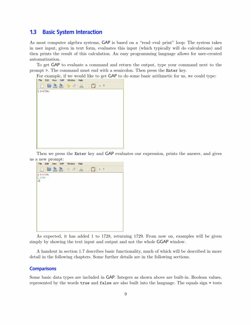
As most computer algebra systems, GAP is based on a “read–eval–print” loop: The system takesin user input, given in text form, evaluates this input (which typically will do calculations) andthen prints the result of this calculation. An easy programming language allows for user-createdautomatization.
To get GAP to evaluate a command and return the output, type your command next to theprompt >. The command must end with a semicolon. Then press the Enter key.
For example, if we would like to get GAP to do some basic arithmetic for us, we could type:
Then we press the Enter key and GAP evaluates our expression, prints the answer, and givesus a new prompt:
As expected, it has added 1 to 1728, returning 1729. From now on, examples will be givensimply by showing the text input and output and not the whole GGAP window.
A handout in section 1.7 describes basic functionality, much of which will be described in moredetail in the following chapters. Some further details are in the following sections.
Comparisons
Some basic data types are included in GAP. Integers as shown above are built-in. Boolean values,represented by the words true and false are also built into the language. The equals sign = tests
9

whether or not two expressions are the same.
gap> 8 = 9;falsegap> 1^3+12^3 = 9^3+10^3;true
The boolean operations and, or, and not are frequently useful. For example:
gap> not (8 = 9 and 2 < 3);true
Variables and Assignment
Any object (or system result) can be stored in a variable. A variable can be thought of as a namewhich points to a particular object that has been computed. The user may pick any name thatis not already a reserved word for the system. The assignment operator is a colon followed by anequals sign, the symbols :=. Once the data is stored in the variable, the variable name may be usedin place of the data. For example:
gap> FirstPerfectNumber:=6;6gap> 22+FirstPerfectNumber;
Notice that the GAP language is not typed and (thanks to a built-in garbage-collector) does notrequire the declaration of the types of variables.
Functions
A function takes as input one or more arguments and may return some output. GAP has manybuilt-in functions. For example, IsPrime takes an integer as its single argument and returns aboolean value, true to indicate the integer is prime and false to indicate it is not.
gap> IsPrime(2^13-1);true
Many many more functions are built into GAP. For information on these, consult the GAP helpfile by typing a question mark followed by the name of the function, or in GGAP click Help on themenu bar.
Additionally, you can define new functions. A function can be defined by writing the wordfunction followed by the arguments and ends with the word end. The word return will returnoutput. For example we can make a function that adds one to an integer:
gap> AddOne:=function(x) return x+1; end;function( x ) ... endgap> AddOne(5);6
10
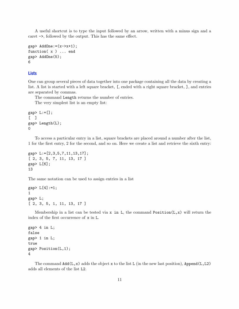
A useful shortcut is to type the input followed by an arrow, written with a minus sign and acaret ->, followed by the output. This has the same effect.
gap> AddOne:=(x->x+1);function( x ) ... endgap> AddOne(5);6
Lists
One can group several pieces of data together into one package containing all the data by creating alist. A list is started with a left square bracket, [, ended with a right square bracket, ], and entriesare separated by commas.
The command Length returns the number of entries.The very simplest list is an empty list:
gap> L:=[];[ ]gap> Length(L);0
To access a particular entry in a list, square brackets are placed around a number after the list,1 for the first entry, 2 for the second, and so on. Here we create a list and retrieve the sixth entry:
gap> L:=[2,3,5,7,11,13,17];[ 2, 3, 5, 7, 11, 13, 17 ]gap> L[6];13
The same notation can be used to assign entries in a list
gap> L[4]:=1;1gap> L;[ 2, 3, 5, 1, 11, 13, 17 ]
Membership in a list can be tested via x in L, the command Position(L,x) will return theindex of the first occurrence of x in L.
gap> 4 in L;falsegap> 1 in L;truegap> Position(L,1);4
The command Add(L,x) adds the object x to the list L (in the new last position), Append(L,L2)adds all elements of the list L2.
11

gap> Add(L,-5);gap> L;[ 2, 3, 5, 1, 11, 13, 17, -5 ]gap> Append(L,[4,3,99,0]);gap> L;[ 2, 3, 5, 1, 11, 13, 17, -5, 4, 3, 99, 0 ]
Lists can contain arbitrary objects, in particular they can contain again lists as entries.
The braces can be used to create subsets of a list, given by a list of index positions:
gap> L[3,5,8];[ 5, 11, -5 ]
A special case of lists are ranges that can be used to store arithmetic progressions in a compactform. The syntax is [start..end] for increments of 1, respectively [start,second..end] forincrements of size second-start. In the folowing example, the surrounding List(...,x->x); isthere purely to force GAP to unpack these compact objects:
gap> List([1..10],x->x);[ 1, 2, 3, 4, 5, 6, 7, 8, 9, 10 ]gap> List([5..12],x->x);[ 5, 6, 7, 8, 9, 10, 11, 12 ]gap> List([5..3],x->x);[ ]gap> List([5,9..45],x->x);[ 5, 9, 13, 17, 21, 25, 29, 33, 37, 41, 45 ]gap> List([10,9..1],x->x);[ 10, 9, 8, 7, 6, 5, 4, 3, 2, 1 ]gap> List([10,9..9],x->x);[ 10, 9 ]gap> L[2..7];[ 3, 5, 1, 11, 13, 17 ]
Lists themselves are pointers to lists – assigning a list to two variables does not make a copyand changing one of the lists will change the other. You can make a new list wityh the same sntriesusing ShallowCopy.
gap> a:=[1,2,3];[ 1, 2, 3 ]gap> b:=a;[ 1, 2, 3 ]gap> c:=ShallowCopy(a);[ 1, 2, 3 ]gap> a[2]:=4;4gap> a;b;c;[ 1, 4, 3 ]
12

[ 1, 4, 3 ][ 1, 2, 3 ]
Vectors and Matrices
Vectors in GAP are simply lists of field elements and matrices are simply lists of their row vectors,i.e. lists of lists. (Thus matrix entries can be accessed as M[row][column].)
While vectors in GAP are usually considered as row vectors, scalar products or matrix/vectorproducts automatically consider the second factor as column vector.
gap> vec:=[-1,2,1];[ -1, 2, 1 ]gap> M:=[[1,2,3],[4,5,6],[7,8,9]];[ [ 1, 2, 3 ], [ 4, 5, 6 ], [ 7, 8, 9 ] ]gap> vec*M;[ 14, 16, 18 ]gap> M*vec;[ 6, 12, 18 ]gap> M[3][2];8gap> vec*vec; # inner product6
The operation Display can be used to print a matrix in a nicely formatted way.
gap> Display(M);[ [ 1, 2, 3 ],[ 4, 5, 6 ],[ 7, 8, 9 ] ]
Matrices and vectors occurring in algorithms are often made immutable, i.e. locked againstchanging entries. (This is made to enable GAP to store certain properties without risking that an en-try change would modify the property.) If it is desired to change the entries ShallowCopy(vector )or MutableCopyMat(matrix ) returns a duplicate object that can be modified.
An example of why this is desirable is seen by the fact that a matrix, being just a list of itsrows, does not copy the rows. Thus for example, assigning the same row to two matriced (or tothe same matrix twice), and then changing this row will change both matrices!
gap> row:=[1,0];[ 1, 0 ]gap> mat1:=[row,[0,1]];[ [ 1, 0 ], [ 0, 1 ] ]gap> mat2:=[row,[0,1]]; # first row is identical, second just equal[ [ 1, 0 ], [ 0, 1 ] ]gap> mat1[2][1]:=3;;mat1;mat2;[ [ 1, 0 ], [ 3, 1 ] ][ [ 1, 0 ], [ 0, 1 ] ]
13

gap> mat1[1][2]:=5;;mat1;mat2;[ [ 1, 5 ], [ 3, 1 ] ][ [ 1, 5 ], [ 0, 1 ] ]
Further linear algebra functionality is decribed in chapter ??.
Sets and sorted lists
Sorted lists (in general GAP implements a total ordering via < on all its objects, though this orderingis sometimes nonobvious for more complicated objects) are used to represent sets in GAP. For a listL, the command Set(L) will return a sorted copy. Element test in sets also used the in operator,but internally then can use binary search for a notable speedup. The same holds for Position.
Maintaining the set property, AddSet(L,x) will insert x into L at the appropriate position tomaintain sortedness. Union(L,L2) and Intersection(L,L2) perform the set operations indicatedby their name, Difference(L,L2) is the set theoretic difference.
gap> L:=Set([5,2,8,9,-3]);[ -3, 2, 5, 8, 9 ]gap> AddSet(L,4);L;[ -3, 2, 4, 5, 8, 9 ]gap> Union(L,[3..6]);[ -3, 2, 3, 4, 5, 6, 8, 9 ]gap> Intersection(L,[3..6]);[ 4, 5 ]gap> Difference(L,[3..6]);[ -3, 2, 8, 9 ]
List operations
GAP contains powerful list operations that often can be used to implement simple programmingtasks in a single line. The typical format for these operations is to give as arguments a list L and afunction func that is to be applied to the entries. These functions often are given in the shorthandform x->expr(x), where expr(x ) is an arbitrary GAP expression, involving x .
List(L ,func ) applies func to all entries of L and returns the list of results.
Filtered(L ,func ) returns the list of those elements of L , for which func returns true.
Number(L ,func ) returns the number of elements of L , for which func returns true.
gap> List([1..10],x->x^2);[ 1, 4, 9, 16, 25, 36, 49, 64, 81, 100 ]gap> Filtered([1..10],IsPrime);[ 2, 3, 5, 7 ]gap> Number([1..10],IsPrime);4
(Note in the first example the function x->x^2 which is such an inline function)
14

gap> x->x^2;function( x ) ... endgap> Print(last);function ( x )return x ^ 2;
end
First(L ,func ) returns the first element of L for which func returns true.
ForAll(L ,func ) returns true if func returns true for all entries of L .
ForAny(L ,func ) similarly returns true if func returns true for at least one entry of L .
Collected(L) returns a statistics of the elements of L in form of a list with entries [object,count].
Sum(L) takes the sum of the entries of L. The variant Sum(L ,func ) sums over the results of func ,applied to the entries of L .
Product(L) takes the product of the entries of L. Again Product(L ,func ) applies func to theentries of L first.
gap> First([1000..2000],IsPrime);1009gap> ForAll([1..10],IsPrime);falsegap> ForAny([1..10],IsPrime);truegap> Collected(List([1..100],IsPrime));[ [ true, 25 ], [ false, 75 ] ]gap> Sum([1..10]);55gap> Sum([1..10],x->x^2);385
Combining these list operations allows for the implementation of small programs. For example,the following commands calculate the first 13 Mersenne numbers, and test which of these are prime.
gap> L:=List([1..13],x->2^x-1);[ 1, 3, 7, 15, 31, 63, 127, 255, 511, 1023, 2047, 4095, 8191 ]gap> Filtered(L, IsPrime );[ 3, 7, 31, 127, 8191 ]
The same can be accomplished in a single command:
gap> Filtered(List([1..13],x->2^x-1),IsPrime);[ 3, 7, 31, 127, 8191 ]
Here we determine a statistics of the last digits of∑ni=1 i
2 for n ≤ 100:
15

gap> Collected(List([1..100],n->Sum([1..n],i->i^2) mod 10));[ [ 0, 30 ], [ 1, 10 ], [ 4, 10 ], [ 5, 30 ], [ 6, 10 ], [ 9, 10 ] ]
For a more involved example, the following construct finds all Carmichael numbers 1 < n ≤ 2000(i.e. those non-primes n such that bn−1 ≡ 1 (mod n)∀b < n : gcd(b, n) = 1).
gap> Filtered( Filtered([2..2000],n->not IsPrime(n)),> n->ForAll( Filtered([2..n-1],b->Gcd(b,n)=1),> b->b^(n-1) mod n=1) );[ 561, 1105, 1729 ]
Basic Programming
GAP includes the basic control structures found in almost any other programming language: loopsand conditional statements.
The basic loop is a for loop. Typically it will repeat some instructions as a variable iteratesthrough all members of a list. The instructions begin with the word do and end with od. To continuewith the example above, suppose we wanted to look at the number of divisors of some Mersennenumbers:
gap> for i in [1..13] do Print("The number of divisorsof 2^",i,"-1 is ",Length(DivisorsInt(2^i-1)),"\n"); od;
The number of divisors of 2^1-1 is 1The number of divisors of 2^2-1 is 2The number of divisors of 2^3-1 is 2The number of divisors of 2^4-1 is 4The number of divisors of 2^5-1 is 2The number of divisors of 2^6-1 is 6The number of divisors of 2^7-1 is 2The number of divisors of 2^8-1 is 8The number of divisors of 2^9-1 is 4The number of divisors of 2^10-1 is 8The number of divisors of 2^11-1 is 4The number of divisors of 2^12-1 is 24The number of divisors of 2^13-1 is 2
In this case, the variable i is iterating over the numbers from 1 to 13. Notice the Print commandand the linebreak \n are used to make the output more readable and to force the system to sendthe printed line to the screen.
A conditional statement begins with if, followed by a boolean, the word then, and a set ofinstructions, and is finished with fi. The instructions are executed if and only if the booleanevaluates to true. Additional conditions and instructions may be given with the elif (with furtherconditions) and else (with no further conditions) commands. For example (one can move input tothe next line without evaluating by pressing Shift+Enter):
gap> PerfectNumber:=function(n)
16

local sigma;sigma:=Sum(DivisorsInt(n));if sigma>2*n then
Print(n," is abundant\n");elif sigma = 2*n then
Print(n," is perfect\n");else
Print(n," is deficient\n");fi;
end;function( n ) ... endgap> PerfectNumber(6);
6 is perfect
Note that the functions Sum and DivisorsInt are built-in to GAP.As a general tip, if a conditional statement is going to be applied to several pieces of data, it is
usually easier to write a function that returns a boolean value and then use the Filtered commandrather than combining loops and conditionals.
1.4 File Operations
For documenting system interactions, transferring results, as well as for preparing programs in afile, it is convenient to have the system read from or write to files. Such files typically will be plaintext files, though GAP itself does not insist on using a specific suffix to indicate the format.
Files and Directories
A filename in GAP is simply a string indicating the location of the file, such as
/Users/xyrxmir/Documents/gapstuff/myprogram/cygdrive/c/Documents and Settings/Administrator/Desktop/myprogram
We note that – regardless of the operating system convention – directories in a path are alwaysseparated by a forward slash /, also under Windows – an inheritance of the cygwin environmentused to run GAP – a drive letter X: is replaced by /cygdrive/x/, i.e. /cygdrive/c/ is the rootdirectory of the system drive.
Directories are simply shortcuts to particular paths. A directory is created by Directory(path ).Then Filename(directory ,filename ) simply produces a string eading with the path of directory .(filename does not need to be a simple file, but actually could include further subdirectories.) Nei-ther Directory, nor Filename check whether the file exists.
gap> dir:=Directory("/Users/xyrxmir/gapstuff");dir("/Users/xyrxmir/gapstuff/")gap> Filename(dir,"stuff");"/Users/xyrxmir/gapstuff/stuff"gap> Filename(dir,"stuffdir/one");
17

"/Users/xyrxmir/gapstuff/stuffdir/one"
Working directories
One difficulty is that these accesses typically act by default on the folder from which GAP wasstarted. When working from a shell, this can easily be arranged to be th working directory. Whenrunning GGAP however, it typically ends up a system or program folder, to which the user mightnot even have access.
It therefore can be crucial to specify suitable directories. Alas specifying the Desktop or userhome folder can be confusing (in particular under Windows), which is where the following twofunctions come into play.
DirectoryHome() returns the user’s home directory. Under Unix this is simply the home folderdenoted by ~user in the shell, under Windows this is the user’s My Documents directory1.
gap> DirectoryHome();dir("/Users/xyrxmir/")gap> DirectoryDesktop();dir("/Users/xyrxmir/Desktop/")
or on a Windows system for example:
DirectoryHome();dir("/cygdrive/c/Documents and Settings/Administrator/My Documents/")DirectoryDesktop();dir("/cygdrive/c/Documents and Settings/Administrator/Desktop/")
Similarly DirectoryDesktop() returns the user’s “Desktop” folder, which under Unix or OSXis defined to be the Desktop directory in the home directory.
At the moment these two functions are in a separate file mydirs.g which needs to be read in first.To avoid a bootstrap issue with directory names, it is most convenient to put this file in GAP’s libraryfolder ( /Applications/gap4r4/lib under OSX, respectively /Program Files/GAP/gap4r4/libunder Windows) to enable simple reading with ReadLib("mydirs.g");
See also section ?? on how to configure automatic reading of functions.
Input and Output
The command PrintTo(filename ,...) works like Print, but prints the output in the file specifiedby filename . The file is created if it did not exist before and any existing file is overwritten.
AppendTo(filename ,...) does the same, but appends the output to an existing file.
GAP can read input using the Read(filename ) command. The contents of the file are read inas if the contents were typed into the system (just not printing out the results of commands).In particular, to read in objects to GAP it is necessary to have lines start with a variable assignmentand end with a semicolon. As with typing, line breaks are typically not relevant.
1or the appropriately named folder in other language versions of Windows. Please be advised that these namesare currently hardcoded into the system and GAP might not support all non-english languages in this yet.
18

The most frequent use of Read is to prepare GAP programs in a text editor and then read theminto the system – this provides far better editing facilities than trying to write the program directlyin the system, see ‘File Input’ below.
A special form of output is provided by the commands LogTo(filename ), LogInputTo(filename ),and LogOutputTo(filename ), which produce a transcript of a system session (respectively onlyinput or output) to the specified file.
logfile:=Filename(DirectoryDesktop(),"mylog");"/cygdrive/c/Documents and Settings/Administrator/Desktop/mylog"LogTo(logfile);
Logging can be stopped by giving no argument to the function.
There are other commands which allow even binary file access, they are described in the refencemanual chapter on streams.
File Input
Often one wants to write more complicated pieces of code and save them for use later. In thissituation it is useful to use your favorite text editor to create a file that GAP can then read.(Caveat: The file must be a plain text file, often denoted by a suffix .txt Programs that can createsuch files are Notepad under Windows and TextEdit under OSX. If you use Word, make sure youuse ‘Save As’ to save as a plain text file.)
Files can be saved elsewhere, but then either the relative path from the root directory or theabsolute path must be typed into the Read command.
For example, one can save our function from above by typing the following text using a texteditor as PerfectNumbers.g in ones home directory:
PerfectNumber:=function(n)local sigma;sigma:=Sum(DivisorsInt(n));if sigma>2*n then
Print(n," is abundant");elif sigma = 2*n then
Print(n," is perfect");else
Print(n," is deficient");fi;
end;
Now any time we run GAP, we can type the command:
gap>Read(Filename(DirectoryHome(),"PerfectNumbers.g"));
Though GAP doesn’t return anything, it has read our text file and now “knows” the functionwe defined. We can now use the function as if we had defined it right in our worksheet.
19

gap>Read("PerfectNumbers.g");
gap> PerfectNumber(6);6 is perfect
1.5 Renaming Objects
(This feature will be available only in GAP 4.5).When introducing new concepts it can be useful to hide any complexity of an object behind a
name (assuming that the object is set up in a file read in by the student which hides all technicalitiesfrom her).
A typical example would be the introduction of the first example of a group, in which theelements have particular names. The easiest way to deal with this situation is to define the objects(and thus their multiplication) via one of GAP’s standard representation, but then simply give aprinting name to the object.
Such display names can be defined by the function SetNameObject. If a is any GAP object,SetNameObject(a,"namestring"); will cause any occurrence of this object to be displayed asnamestring.
gap> SetNameObject(4,"four");gap> List([1..5],x->x^2);[ 1, four, 9, 16, 25 ]
This change of course is restricted to the display, as the object stays the same – setting a namethus will not affect any calculations.
Section 3.3 contains a more involved example of using this feature in creating a group whoseobjects are (to the student) simply given by names.
Note that setting a printing name will not automatically define the corresponding variable.Also the change of name only arises in View (the default function used to display objects after acommand) and not in an explicit Print.
The implementation of this feature relies on checking any object to be displayed in a table forit haveing been given a particular name. Naming more than a few dozen objects thus could lead toa notable slowdown.
1.6 Teaching Mode
Some of the internal workings of GAP are not obvious and the representation of certain objectscan only be understood with a substantial knowledge of algebra. Still, often there is an easierunderstood (just not as efficient) representation of such objects that is feasible for beginning users.
Similarly, GAP is lacking routines for certain mathematical properties, because the only knownalgorithms are very naive, run slowly and scale badly; or because the results for all but trivialexamples would be so large to be practically meaningless. Still, trivial examples can be meaningfulin a teaching context.
To enable this kind of functionality, GAP offers a teaching mode. It is turned on by the commandTeachingMode(true); Once this is done, GAP simplifies the display of certain objects (potentially
20

at the cost of making the printing of objects more expensive); it also enables naive routines forsome calculations.
This book will describe these modifications in the context of the topics.
1.7 Handouts
Introduction to GAP
Note: This handout contains many section, not all relevant for every course. Cut as needed.
You can start GAP with the ggap icon (in Windows on the desktop, under OSX in the Applicationsfolder), under Unix you call the gap.sh batch file in the gap4r4/bin directory. The program willstart up and you will get window into which you can input text at a prompt >. We will write thisprompt here as gap> to indicate that it is input to the program.
gap>
You now can type in commands (followed by a semicolon) and GAP will print out the result.To leave GAP you can either call quit; or close the window.You should be able to use the mouse and cursor keys for editing lines. (In the text version
under Unix, the standard EMACS keybindings are accepted.) Note that changing prior entries inthe worksheet does not change the prior calculation, but just executes the same command again.If you want to repeat a sequence of commands, pasting the lines in is a better approach.
You can use the online help with ? to get documentation for particular commands.
gap> ?gcd
A double question mark ?? checks for keywords or parts of command names. If multiple sectionsapply GAP will list all of them with numbers, one can simply type ?number to get a particularsection.
gap> ??gcdHelp: several entries match this topic (type ?2 to get match [2])[1] Reference: Gcd[2] Reference: Gcd and Lcm[3] Reference: GcdInt[4] Reference: Gcdex[5] Reference: GcdOp[6] Reference: GcdRepresentation[7] Reference: GcdRepresentationOp[8] Reference: TryGcdCancelExtRepPolynomials[9] GUAVA (not loaded): DivisorGCDgap> ?6
You might want to create a transcript of your session in a text file. You can do this by issuingthe command LogTo(filename ); Note that the filename must include the path to a user writabledirectory. Under Windows
21

• Paths are always given with a forwards slash (/), even though the operating system uses abackslash.
• Instead of drive letters, the prefix /cygdrive/letter is used, e.g. /cygdrive/c/ is the maindrive.
• It can be convenient to use DirectoryDesktop() or DirectoryHome() to create a file on thedesktop or in the My Documents folder.
LogTo("mylog")LogTo("/cygdrive/c/Documents and Settings/Administrator/My Documents/logfile.txt");LogTo(Filename(DirectoryDesktop(),"logfile.txt"));
You can end logging with the command
LogTo();
Some general hints:
• GAP is picky about upper case/lower case. LogTo is not the same as logto.
• All commands end in a semicolon.
• If you create larger input, it can be helpful to put it in a text file and to read it from GAP. Thiscan be done with the command Read("filename"); – the same issues about paths apply.
• By terminating a command with a double semicolon ;; you can avoid GAP displaying theresult. (Obviously, this is only useful if assigning it to a variable.)
• everything after a hash mark (#) is a comment.
We now do a few easy calculations. If you have not used GAP before, it might be useful to dothese on the computer in parallel to reading.
Integers and Rationals GAP knows integers of arbitrary length and rational numbers:
gap> -3; 17 - 23;-3-6gap> 2^200-1;1606938044258990275541962092341162602522202993782792835301375gap> 123456/7891011+1;2671489/2630337
The ‘mod’ operator allows you to compute one value modulo another. Note the blanks:
gap> 17 mod 3;2
GAP knows a precedence between operators that may be overridden by parentheses and can compareobjects:
22

gap> (9 - 7) * 5 = 9 - 7 * 5;falsegap> 5/3<2;true
You can assign numbers (or more general: every GAP object) to variables, by using the assignmentoperator :=. Once a variable is assigned to, you can refer to it as if it was a number. The specialvariables last, last2, and last3 contain the results of the last three commands.
gap> a:=2^16-1; b:=a/(2^4+1);655353855gap> 5*b-3*a;-177330gap> last+5;-177325gap> last+2;-177323
The following commands show some useful integer calculations related to quotient and remain-der:
gap> Int(8/3); # round down2gap> QuoInt(76,23); # integral part of quotient3gap> QuotientRemainder(76,23);[ 3, 7 ]gap> 76 mod 23; # remainder (note the blanks)7gap> 1/5 mod 7;3gap> Gcd(64,30);2gap> rep:=GcdRepresentation(64,30);[ -7, 15 ]gap> rep[1]*64+rep[2]*30;2gap> Factors(2^64-1);[ 3, 5, 17, 257, 641, 65537, 6700417 ]
Lists Objects separated by commas and enclosed in square brackets form a list.Any collections of objects, including sets, are represented by such lists. (A Set in GAP is a
sorted list.)
gap> l:=[5,3,99,17,2]; # create a list[ 5, 3, 99, 17, 2 ]
23

gap> l[4]; # access to list entry17gap> l[3]:=22; # assignment to list entry22gap> l;[ 5, 3, 22, 17, 2 ]gap> Length(l);5gap> 3 in l; # element testtruegap> 4 in l;falsegap> Position(l,2);5gap> Add(l,17); # extension of list at endgap> l;[ 5, 3, 22, 17, 2, 17 ]gap> s:=Set(l); # new list, sorted, duplicate free[ 2, 3, 5, 17, 22 ]gap> l;[ 5, 3, 22, 17, 2, 17 ]gap> AddSet(s,4); # insert in sorted positiongap> AddSet(s,5); # and avoid duplicatesgap> s;[ 2, 3, 4, 5, 17, 22 ]
Results that consist of several numbers typically are represented as a list.
gap> DivisorsInt(96);[ 1, 2, 3, 4, 6, 8, 12, 16, 24, 32, 48, 96 ]gap> Factors(2^126-1);[ 3, 3, 3, 7, 7, 19, 43, 73, 127, 337, 5419, 92737, 649657, 77158673929 ]
There are powerful list functions that often can save programming loops: List, Filtered,ForAll, ForAny, First. They take as first argument a list, and as second argument a function tobe applied to the list elements or to test the elements. The notation i -> xyz is a shorthand for aone parameter function.
gap> l:=[5,3,99,17,2];[ 5, 3, 99, 17, 2 ]gap> List(l,IsPrime);[ true, true, false, true, true ]gap> List(l,i -> i^2);[ 25, 9, 9801, 289, 4 ]gap> Filtered(l,IsPrime);[ 5, 3, 17, 2 ]gap> ForAll(l,i -> i>10);
24

falsegap> ForAny(l,i -> i>10);truegap> First(l,i -> i>10);99
A special case of lists are ranges, indicated by double dots. They can also be used to createarithmetic progressions:
gap> l:=[10..100];[ 10 .. 100 ]gap> Length(l);91
Polynomials To create polynomials, we need to create the variable first. Note that the name wegive is the printed name (which could differ from the variable we assign it to). As GAP does notknow the real numbers we do it over the rationals
gap> x:=X(Rationals,"x");x
If we wanted, we could define several different variables this way. Now we can do all the usualarithmetic with polynomials:
gap> f:=x^7+3*x^6+x^5+3*x^3-4*x^2-4*x;x^7+3*x^6+x^5+3*x^3-4*x^2-4*xgap> g:=x^5+2*x^4-x^2-2*x;x^5+2*x^4-x^2-2*xgap> f+g;f*g;x^7+3*x^6+2*x^5+2*x^4+3*x^3-5*x^2-6*xx^12+5*x^11+7*x^10+x^9-2*x^8-5*x^7-14*x^6-11*x^5-2*x^4+12*x^3+8*x^2
The same operations as for integers hold for polynomials
gap> QuotientRemainder(f,g);[ x^2+x-1, 3*x^4+6*x^3-3*x^2-6*x ]gap> f mod g;3*x^4+6*x^3-3*x^2-6*xgap> Gcd(f,g);x^3+x^2-2*xgap> GcdRepresentation(f,g);[ -1/3*x, 1/3*x^3+1/3*x^2-1/3*x+1 ]gap> rep:=GcdRepresentation(f,g);[ -1/3*x, 1/3*x^3+1/3*x^2-1/3*x+1 ]gap> rep[1]*f+rep[2]*g;x^3+x^2-2*xgap> Factors(g);[ x-1, x, x+2, x^2+x+1 ]
25

Vectors and Matrices Lists are also used to form vectors and matrices:A vector is simply a list of numbers. A list of (row) vectors is a matrix. GAP knows matrix
arithmetic.
gap> vec:=[1,2,3,4];[ 1, 2, 3, 4 ]gap> vec[3]+2;5gap> 3*vec+1;[ 4, 7, 10, 13 ]gap> mat:=[[1,2,3,4],[5,6,7,8],[9,10,11,12]];[ [ 1, 2, 3, 4 ], [ 5, 6, 7, 8 ], [ 9, 10, 11, 12 ] ]gap> mat*vec;[ 30, 70, 110 ]gap> mat:=[[1,2,3],[5,6,7],[9,10,12]];;gap> mat^5;[ [ 289876, 342744, 416603 ], [ 766848, 906704, 1102091 ],[ 1309817, 1548698, 1882429 ] ]
gap> DeterminantMat(mat);-4
The command Display can be used to get a nicer output:
gap> 3*mat^2-mat;[ [ 113, 130, 156 ], [ 289, 342, 416 ], [ 492, 584, 711 ] ]gap> Display(last);[ [ 113, 130, 156 ],[ 289, 342, 416 ],[ 492, 584, 711 ] ]
Roots Of Unity The expression E(n) is used to denote the n-th root of unity (e2πin ):
gap> root5:=E(5)-E(5)^2-E(5)^3+E(5)^4;;gap> root5^2;5
Finite Fields To compute in finite fields, we have to create special objects to represent theresidue classes (Internally, GAP uses so-called Zech Logarithms and represents all nonzero elementsas power of a generator of the cyclic multiplicative group.)
gap> gf:=GF(7);GF(7)gap> One(gf);Z(7)^0gap> a:=6*One(gf);Z(7)^3gap> b:=3*One(gf);
26

Z(7)gap> a+b;Z(7)^2gap> Int(a+b);2
Non-prime finite fields are created in the same way with prime powers, note that GAP automaticallyrepresents elements in the smallest field possible.
gap> Elements(GF(16));[ 0*Z(2), Z(2)^0, Z(2^2), Z(2^2)^2, Z(2^4), Z(2^4)^2, Z(2^4)^3, Z(2^4)^4,Z(2^4)^6, Z(2^4)^7, Z(2^4)^8, Z(2^4)^9, Z(2^4)^11, Z(2^4)^12, Z(2^4)^13,Z(2^4)^14 ]
We can also form matrices over finite fields.
gap> mat:=[[1,2,3],[5,6,7],[9,10,12]]*One(im);[ [ Z(7)^0, Z(7)^2, Z(7) ], [ Z(7)^5, Z(7)^3, 0*Z(7) ],[ Z(7)^2, Z(7), Z(7)^5 ] ]
gap> mat^-1+mat;[ [ Z(7)^4, Z(7)^4, Z(7)^4 ], [ Z(7)^3, Z(7)^0, Z(7)^5 ],[ Z(7), Z(7)^0, Z(7)^3 ] ]
Integers modulo If we want to compute in the integers modulo n (what we called Zn in thelecture) without need to always type mod we can create obhjects that immediately reduce theirarithmetic modulo n:
gap> im:=Integers mod 6; # represent numbers for ‘‘modulo 6’’ calculations(Integers mod 6)
To convert “ordinary” integers to residue classes, we have to multiply them with the“One” of theseresidue classes, the command Int converts back to ordinary integers:
gap> a:=5*One(im);ZmodnZObj( 5, 6 )gap> b:=3*One(im);ZmodnZObj( 3, 6 )gap> a+b;ZmodnZObj( 2, 6 )gap> Int(last);2
(If one wants one can get all residue classes or – for example test which are invertible).
gap> Elements(im);[ ZmodnZObj(0,6),ZmodnZObj(1,6),ZmodnZObj(2,6),ZmodnZObj(3,6),ZmodnZObj(4,6),ZmodnZObj(5,6) ]
gap> Filtered(last,x->IsUnit(x));[ ZmodnZObj( 1, 6 ), ZmodnZObj( 5, 6 ) ]
27

gap> Length(last);2
If we calculate modulo a prime the default output looks a bit different.
gap> im:=Integers mod 7;GF(7)
(The name GF stands for Galois Field, explanation later.) Also elements display differently. There-fore it is convenient to once issue the command
gap> TeachingMode(true);
which (amongst others) will simplify the display.
Matrices and Polynomials modulo a prime We can use these rings to calculate in matricesmodulo a number. Display again brings it into a nice form:
gap> mat:=[[1,2,3],[5,6,7],[9,10,12]]*One(im);[ [ ZmodnZObj( 1, 7 ), ZmodnZObj( 2, 7 ), ZmodnZObj( 3, 7 ) ],[ ZmodnZObj( 5, 7 ), ZmodnZObj( 6, 7 ), ZmodnZObj( 0, 7 ) ],[ ZmodnZObj( 2, 7 ), ZmodnZObj( 3, 7 ), ZmodnZObj( 5, 7 ) ] ]
gap> Display(mat);1 2 35 6 .2 3 5gap> mat^-1+mat;[ [ ZmodnZObj( 4, 7 ), ZmodnZObj( 4, 7 ), ZmodnZObj( 4, 7 ) ],[ ZmodnZObj( 6, 7 ), ZmodnZObj( 1, 7 ), ZmodnZObj( 5, 7 ) ],[ ZmodnZObj( 3, 7 ), ZmodnZObj( 1, 7 ), ZmodnZObj( 6, 7 ) ] ]
In the same way we can also work with polynomials modulo a number. For this one just needsto define a suitable variable. For example suppose we want to work with polynomials modulo 2:
gap> r:=Integers mod 2;GF(2)gap> x:=X(r,"x");xgap> f:=x^2+x+1;x^2+x+Z(2)^0gap> Factors(f);[ x^2+x+Z(2)^0 ]
As 2 is a prime (and therefore every nonzero remainder invertible), we can now work withpolynomials modulo f . The possible remainders now are all the polynomials of strictly smallerdegree (with coefficients suitable reduced):
28

gap> o:=One(r);Z(2)^0gap> elms:=[0*x,0*x+o,x,x+o];[ 0*Z(2), Z(2)^0, x, x+Z(2)^0 ]
We can now build addition and multiplication tables for these four objects modulo f :
gap> Display(List(elms,a->List(elms,b->Position(elms,a+b mod f))));[ [ 1, 2, 3, 4 ],[ 2, 1, 4, 3 ],[ 3, 4, 1, 2 ],[ 4, 3, 2, 1 ] ]
gap> Display(List(elms,a->List(elms,b->Position(elms,a*b mod f))));[ [ 1, 1, 1, 1 ],[ 1, 2, 3, 4 ],[ 1, 3, 4, 2 ],[ 1, 4, 2, 3 ] ]
Groups and Homomorphisms We can write permutations in cycle form and multiply (or invertthem):
gap> a:=(1,2,3,4)(6,5,7);(1,2,3,4)(5,7,6)gap> a^2;(1,3)(2,4)(5,6,7)gap> a^-1;(1,4,3,2)(5,6,7)gap> b:=(1,3,5,7)(2,6,8);; a*b;
Note: GAP multiplies permutations from left to right, i.e. (1, 2, 3) · (2, 3) = (1, 3). (This mightdiffer from what you used in prior courses.)
A group is generated by the command Group, applied to generators (permutations or matrices).It is possible to compute things such as Elements, group Order or ConjugacyClasses.
gap> g:=Group((1,2,3,4,5),(2,5)(3,4));Group([ (1,2,3,4,5), (2,5)(3,4) ])gap> Elements(g);[ (), (2,5)(3,4), (1,2)(3,5), (1,2,3,4,5), (1,3)(4,5), (1,3,5,2,4),(1,4)(2,3), (1,4,2,5,3), (1,5,4,3,2), (1,5)(2,4) ]
gap> Order(g);10gap> c:=ConjugacyClasses(g);[ ()^G, (2,5)(3,4)^G, (1,2,3,4,5)^G, (1,3,5,2,4)^G ]gap> List(c,Size);[ 1, 5, 2, 2 ]gap> List(c,Representative);[ (), (2,5)(3,4), (1,2,3,4,5), (1,3,5,2,4) ]
29

Homomorphisms can be created by giving group generators and their images under the map.(GAP will check that the map indeed defines a homomorphism first. One can use GroupHomomorphismByImagesNCto skip this test.)
gap> g:=Group((1,2,3),(3,4,5));;gap> mat1:=[ [ 0, -E(5)-E(5)^4, E(5)+E(5)^4 ], [ 0, -E(5)-E(5)^4, -1 ],> [ 1, 1, E(5)+E(5)^4 ] ];;gap> mat2:=[ [ 1, 0, E(5)+E(5)^4 ], [ -E(5)-E(5)^4, 0, E(5)+E(5)^4 ],> [ -E(5)-E(5)^4, -1, -1 ] ];;gap> img:=Group(mat1,mat2);;gap> hom:=GroupHomomorphismByImages(g,img,[(1,2,3),(3,4,5)],[mat1,mat2]);[ (1,2,3), (3,4,5) ] ->[ [[0,-E(5)-E(5)^4,E(5)+E(5)^4],[0,-E(5)-E(5)^4,-1],[1,1,E(5)+E(5)^4]],[[1,0,E(5)+E(5)^4],[-E(5)-E(5)^4,0,E(5)+E(5)^4],[-E(5)-E(5)^4,-1,-1]] ]
gap> Image(hom,(1,2,3,4,5));[ [E(5)+E(5)^4,0,1], [E(5)+E(5)^4,1,0], [ -1, 0, 0 ] ]gap> r:=[ [ 1, E(5)+E(5)^4, 0 ], [ 0, E(5)+E(5)^4, 1 ], [ 0, -1, 0 ] ];;gap> PreImagesRepresentative(hom,r);(1,4,2,3,5)
Group Actions The general setup for group actions is to give:
• The acting group
• The domain (this is optional if one calculates the Orbit of a point
• In the case of computing an orbit, the staring point ω
• (There is the option to give group generators and acting images as extra argument. For themoment just forget it.)
• A function f(ω, g) that is used to compute ωg. If not given the function OnPoints, whichreturns ω^g, is used.
Common functions are: Orbit, Orbits, Stabilizer. The function ActionHomomorphism can beused to compute a homomorphism into SΩ given by the permutation action.
gap> Orbit(g,1);[ 1, 2, 3, 4 ]gap> Orbit(g,[1,2],OnSets);[ [ 1, 2 ], [ 2, 3 ], [ 3, 4 ], [ 1, 3 ], [ 1, 4 ], [ 2, 4 ] ]gap> Orbit(g,[1,2],OnTuples);[ [ 1, 2 ], [ 2, 3 ], [ 2, 1 ], [ 3, 4 ], [ 1, 3 ], [ 3, 2 ], [ 4, 1 ],[ 2, 4 ], [ 4, 3 ], [ 3, 1 ], [ 4, 2 ], [ 1, 4 ] ]
gap> Orbits(Group((1,2,3,4),(1,3)(2,4)),Combinations([1..4],2),OnSets);[ [ [ 1, 2 ], [ 2, 3 ], [ 3, 4 ], [ 1, 4 ] ],
[ [ 1, 3 ], [ 2, 4 ] ] ]gap> Stabilizer(g,1);Group([ (2,3,4), (3,4) ])
30

1.8 Problems
Exercise 1. In mathematics, a common strategy is to use a computer to gather data in small cases,notice a pattern, and then try to prove things in general once a pattern is found. We will try thistactic here.
As in the conditional example, a positive integer n is called a perfect number if and only if thesum of the divisors of n equals 2n, or equivalently the sum of the proper divisors of n equals n.
a) Write a function that takes a positive integer n as input and returns true if n is perfect andfalse if n is not perfect.
b) Use your function to find all perfect numbers less than 1000.c) Notice that all of the numbers you found have a certain form, namely 2n(2n+1− 1) for some
integer n. Are all numbers of this form perfect?d) By experimenting in GAP, conjecture a necessary and sufficient condition for 2n(2n+1 − 1)
to be a perfect number.e) Prove your conjecture is correct.
31

2
-
Rings
Many newer abstract algebra courses start with rings in favour of groups. This has the advantagethat the objects one works with initially – integers, rationals, polynomials, prime fields, are known,or can be easily defined.
Most of these known rings however are infinite and structural information (e.g. units, all ideals)is either known from theorems, or computationally very hard to infeasible. Initial use of GAPtherefore is likely to be as a tool for arithmetic.
2.1 Integers, Rationals and Complex Numbers
There are several rings which teams will have seen before (and therefore know the rules for arith-metic), even if they were not designated as ”ring” at that point. GAP implements many of these.
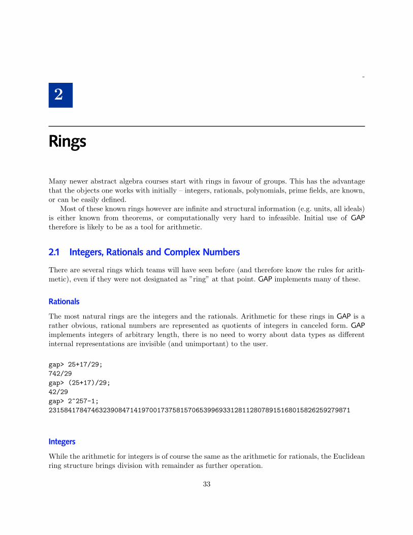
Rationals
The most natural rings are the integers and the rationals. Arithmetic for these rings in GAP is arather obvious, rational numbers are represented as quotients of integers in canceled form. GAPimplements integers of arbitrary length, there is no need to worry about data types as differentinternal representations are invisible (and unimportant) to the user.
gap> 25+17/29;742/29gap> (25+17)/29;42/29gap> 2^257-1;231584178474632390847141970017375815706539969331281128078915168015826259279871
Integers
While the arithmetic for integers is of course the same as the arithmetic for rationals, the Euclideanring structure brings division with remainder as further operation.
33
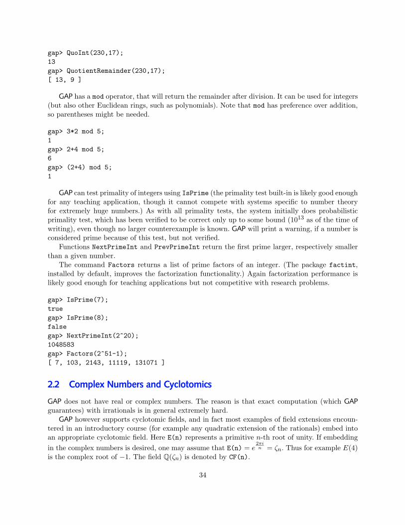
gap> QuoInt(230,17);13gap> QuotientRemainder(230,17);[ 13, 9 ]
GAP has a mod operator, that will return the remainder after division. It can be used for integers(but also other Euclidean rings, such as polynomials). Note that mod has preference over addition,so parentheses might be needed.
gap> 3*2 mod 5;1gap> 2+4 mod 5;6gap> (2+4) mod 5;1
GAP can test primality of integers using IsPrime (the primality test built-in is likely good enoughfor any teaching application, though it cannot compete with systems specific to number theoryfor extremely huge numbers.) As with all primality tests, the system initially does probabilisticprimality test, which has been verified to be correct only up to some bound (1013 as of the time ofwriting), even though no larger counterexample is known. GAP will print a warning, if a number isconsidered prime because of this test, but not verified.
Functions NextPrimeInt and PrevPrimeInt return the first prime larger, respectively smallerthan a given number.
The command Factors returns a list of prime factors of an integer. (The package factint,installed by default, improves the factorization functionality.) Again factorization performance islikely good enough for teaching applications but not competitive with research problems.
gap> IsPrime(7);truegap> IsPrime(8);falsegap> NextPrimeInt(2^20);1048583gap> Factors(2^51-1);[ 7, 103, 2143, 11119, 131071 ]
2.2 Complex Numbers and Cyclotomics
GAP does not have real or complex numbers. The reason is that exact computation (which GAPguarantees) with irrationals is in general extremely hard.
GAP however supports cyclotomic fields, and in fact most examples of field extensions encoun-tered in an introductory course (for example any quadratic extension of the rationals) embed intoan appropriate cyclotomic field. Here E(n) represents a primitive n-th root of unity. If embeddingin the complex numbers is desired, one may assume that E(n) = e
2πin = ζn. Thus for example E(4)
is the complex root of −1. The field Q(ζn) is denoted by CF(n).
34

The command ComplexConjugate(x) can be used to determine the complex conjugate of acyclotomic number.
gap> (2+E(4))^2;3+4*E(4)gap> E(3)+E(3)^2;-1gap> ComplexConjugate(E(7)^2);E(7)^5gap> 1/((1+ER(5))/2);E(5)+E(5)^4
As the last example shows, apart from small cases such as Z[i] = CF(4), the representation ofcyclotomic elements is not always obvious (the reason is the choice of the basis, which for efficiencyreasons does not only consist of the low powers of a primitive root), though rational results willalways be represented as rational numbers.
Quadratic Extensions of the Rationals
Because any quadratic irrationality is cyclotomic, the function ER(n) represents√n as cyclotomic
number.
gap> ER(3);-E(12)^7+E(12)^11gap> 1+ER(3);-E(12)^4-E(12)^7-E(12)^8+E(12)^11gap> (1+ER(2))^2-2*ER(2);3
If teaching mode is turned on, the display of quadratic irrationalities utilizes the ER notation,representing these irrationalities in the natural basis.
gap> 1/(2+ER(3));2-ER(3)
We will see in the chapter on fields how other field extensions can be represented.
2.3 Greatest common divisors and Factorization
The gcd of two numbers can be computed with Gcd. The teaching function ShowGcd performs theextended euclidean algorithm, displaying also how to express the gcd as integer linear combinationof the original arguments
gap> Gcd(192,42);6gap> ShowGcd(192,42);192=4*42 + 2442=1*24 + 18
35

24=1*18 + 618=3*6 + 0The Gcd is 6= 1*24 -1*18= -1*42 + 2*24= 2*192 -9*42
6
GcdRepresentation returns a list [s, t] of the the coefficients from the extended euclideanalgorithm.
gap> a:=GcdRepresentation(192,42);[ 2, -9 ]gap> a[1]*192+a[2]*42;6
2.4 Modulo Arithmetic
The mod-operator can be used in general for arithmetic in the quotient ring. When applied to aquotient of elements, it automatically tries to invert the denominator, using the euclidean algorithm.
gap> 3/2 mod 5;4
Contrary to systems such as Maple, mod is an ordinary binary operator in GAP and does notchange the calculation done before, i.e. calculating (5+3*19) mod 2 first calculates 5+3*19 overthe integers, and then reduces the result. If intermediate coefficient growth is an issue, arguments(and intermediate results) have to be reduced always with mod, e.g. (in the most extreme case) (5mod 2)+((3 mod 2)*(19 mod 2)) mod 2. The function PowerMod(base,exponent,modulus) canbe used to calculate ab mod m with intermediate reduction.
Further Modulo Functionality for Number Theory Courses is described in chapter 6
Checksum Digits
Initial examples for modulo arithmetic often involve checksum digits, and special functions areprovided that perform such calculations for common checksums.
The following functions all accept as input a number, either as integer (though this will notwork properly for numbers with a leading zero!), a string representing an number, a list of digits(as list), or simply the digits separated by commas. (For own code, the function ListOfDigitsaccepts any such input and always returns a list of the digits.)
If a full number, including check digit is given, the check digit is verified and true or falsereturned accordingly. If a number without check digit is given, the check digit is computed andreturned.
CheckDigitISBN works for “classical” 10-digit ISBN numbers. As the arithmetic is modulo 11,an upper case ‘X’ is accepted for check digit 10.
gap> CheckDigitISBN("052166103");
36

Check Digit is ’X’’X’gap> CheckDigitISBN("052166103X");Checksum test satisfiedtruegap> CheckDigitISBN("0521661031");Checksum test failedfalsegap> CheckDigitISBN(0,5,2,1,6,6,1,0,3,1);Checksum test failedfalsegap> CheckDigitISBN(0,5,2,1,6,6,1,0,3,’X’); # note single quotes!Checksum test satisfiedtruegap> CheckDigitISBN(0,5,2,1,6,6,1,0,3);Check Digit is ’X’’X’gap> CheckDigitISBN([0,5,2,1,6,6,1,0,3]);Check Digit is ’X’’X’
CheckDigitISBN13 computes the newer ISBN-13. (The relation to old ISBN is to omit theoriginal check digit, prefix 978 and compute a new check digit with multiplcation factors 1 and 3only for consistency with UPC bar codes.)
gap> CheckDigitISBN13("978052166103");Check Digit is 44gap> CheckDigitISBN13("9781420094527");Checksum test satisfiedtrue
CheckDigitUPC computes checksums for 12-digit UPC codes as used in most stores.
gap> CheckDigitUPC("071641830011");Checksum test satisfiedtruegap> CheckDigitUPC("07164183001");Check Digit is 11
CheckDigitPostalMoneyOrder finally works on 11-digit numbers for (US mail) postal moneyorders.
gap> CheckDigitPostalMoneyOrder(1678645715);Check Digit is 55
37

Similar checksum schemes that check∑ni=1 ciai
∼= 0 (mod m) for a number a1, a2, . . . , an(an being the check digit) and coefficients ci (i.e. for the 10 digit ISBN, the coefficients are[1, 2, 3, 4, 5, 6, 7, 8, 9,−1]) can be created using the function CheckDigitTestFunction(n,modulus,clist ),where clist is a list of the ci. This function returns the actual tester function, i.e. CheckDigitISBNis defined as
CheckDigitISBN:=CheckDigitTestFunction(10,11,[1,2,3,4,5,6,7,8,9,-1]);
2.5 Residue Class Rings and Finite Fields
To avoid any issues with an immediate reduction, in particular in longer calculations, as well as torecognize zero appropriately, it quickly becomes desirable to use different objects which representresidue classes of modulo arithmetic. In the case of the integers, such an object can be created alsowith the mod operator.
gap> a:=Integers mod 6;(Integers mod 6)
The elements of this structure are residue classes, for which arithmetic is defined on the represen-tatives with subsequent reduction:
gap> e[4]+e[6]; #3+5 mod 6ZmodnZObj( 2, 6 )gap> e[4]/e[6]; #3/5 mod 6ZmodnZObj( 3, 6 )
The easiest way to create such residue classes is to multiply a representing integer with the One ofthe residue class ring. Similarly Int returns the canonical representative.
gap> one:=One(a);ZmodnZObj( 1, 6 )gap> 5*one;ZmodnZObj( 5, 6 )gap> Int(10*one);4
It is important to realize that these objects are genuinely different from the integers. If we comparewith integers, GAP considers them to be different objects. To write generic code, one can use thefunctions IsOne and IsZero.
gap> one=1;falsegap> 0*one=0;falsegap> IsZero(0*one);true
38

If we work modulo a prime, the display of objects changes. The reason for this is that finite fieldsare represented internally in a different format. (Elements are represented as powers of a primitiveelement, the multiplicative group of the field being cyclic. This makes multiplication much easier,addition is done using so-called Zech-logarithms, storing x + 1 for every x.) Still, arithmetic andconversion work in the same way as described before.
gap> a:=Integers mod 7;GF(7)gap> Elements(a);[ 0*Z(7), Z(7)^0, Z(7), Z(7)^2, Z(7)^3, Z(7)^4, Z(7)^5 ]gap> 2*one*5*one;Z(7)gap> Int(last);3
As this example shows, the display of an object does not any longer give immediate indication ofthe integer representative.
A further advantage of this different representation for finite fields is that it works as well fornon-prime fields. For any prime-power (up to 216) we can create the finite field of that size. GAPknows about the inclusion relation amongst the fields, and automatically represents elements in thesmallest subfield.
gap> a:=GF(64);GF(2^6)gap> Elements(a);[ 0*Z(2), Z(2)^0, # elements of GF(2)Z(2^2), Z(2^2)^2, # further elements of GF(4)Z(2^3), Z(2^3)^2, Z(2^3)^3, Z(2^3)^4, Z(2^3)^5, Z(2^3)^6, #elts of GF(8)Z(2^6), Z(2^6)^2, Z(2^6)^3, Z(2^6)^4, Z(2^6)^5, Z(2^6)^6, Z(2^6)^7,... # the rest is elements of GF(64) not in any proper subfield.Z(2^6)^57, Z(2^6)^58, Z(2^6)^59, Z(2^6)^60, Z(2^6)^61, Z(2^6)^62 ]
Of course only elements of the prime field have an integer correspondent. Other elements can beidentified with different representations for example using minimal polynomials.
Teaching Mode In teaching mode, display of finite field elements defaults to the ZmodnZObjnotation even for prime fields, also converting the result of ZmodnZObj(n,p) internally back ton*Z(p)^0. Elements of larger finite fields are still displayed in the Z(q) notation.
gap> Elements(GF(9));[ ZmodnZObj( 0, 3 ), ZmodnZObj( 1, 3 ), ZmodnZObj( 2, 3 ), Z(9)^1, Z(9)^2,Z(9)^3, Z(9)^5, Z(9)^6, Z(9)^7 ]
2.6 Arithmetic Tables
A basic way to describe the algebraic structure of small objects, in particular when introducing thetopic, is to give an addition and multiplication table.
39

The commands ShowAdditionTable(obj ) and ShowMultiplicationTable(obj ) will printsuch tables, obj being a list of elements or a structure.
Note that the routines assume that the screen is wide enough to print the whole table. (To makebest use of screen real estate, the routines abbreviate “ZmodnZObj” to “ZnZ” and “<identity ...>’’ to ‘‘\verb¡id¿”.)
gap> ShowAdditionTable(GF(3));+ | ZnZ(0,3) ZnZ(1,3) ZnZ(2,3)---------+---------------------------ZnZ(0,3) | ZnZ(0,3) ZnZ(1,3) ZnZ(2,3)ZnZ(1,3) | ZnZ(1,3) ZnZ(2,3) ZnZ(0,3)ZnZ(2,3) | ZnZ(2,3) ZnZ(0,3) ZnZ(1,3)
gap> ShowMultiplicationTable(GF(3));* | ZnZ(0,3) ZnZ(1,3) ZnZ(2,3)---------+---------------------------ZnZ(0,3) | ZnZ(0,3) ZnZ(0,3) ZnZ(0,3)ZnZ(1,3) | ZnZ(0,3) ZnZ(1,3) ZnZ(2,3)ZnZ(2,3) | ZnZ(0,3) ZnZ(2,3) ZnZ(1,3)
(Caveat: MultiplicationTable is defined separately and returns the table as an integer matrix,indicating the position of the product in the element list)
Section 2.8 describes how to create a ring from addition and multiplication tables, section 3.7describes how to create a group from a multiplication table.
2.7 Polynomials
In contrast to systems such as Maple, GAP does not use undefined variables as elements of apolynomial ring, but one needs to create indeterminates1 explicitly. The polynomial rings in whichthese variables live are (implictly) the polynomial rings in countably many indeterminates overthe cylotomics, the algebraic closures of GF(p) or over other rings. These huge polynomial ringshowever do not need to be created as objects by the user to enable polynomial arithmetic, thoughthe user can create certain polynomial rings if she so desires. (GAP actually implements the quotientfield, i.e. it is possible to form rational functions as quotients of polynomials.)
By default variables are labelled with index numbers, it is possible to assign them names forprinting.
Indeterminates are created by the command Indeterminate which is synonymous with the themuch easier to type X.
gap> x:=X(Rationals); # creates an indeterminate (with index 1)x_1gap> x:=X(Rationals,2); # creates the indeterminate with index 2x_2
By specifying a string as the second argument, an indeterminate is selected and given a name.(Indeterminates are selected from so far unnamed ones, i.e. the first indeterminate that is given aname is index 1.)
1we will prefer the name “indeterminates”, to indicate the difference to global or local variables
40

gap> x:=X(Rationals,"x");xgap> x:=X(Rationals,1); # this is in fact the variable with index 1.xgap> y:=X(Rationals,"y");y
There is no formal requirement to assign indeterminates to variables with the same name, it is goodpractice to avoid confusion.
Polynomials then can be created simply from arithmetic in the variables. (Terms will be rear-ranged internally by GAP to degree-lexicographic ordering to ensure unique storage.)
gap> 5*x*y^5+3*x^4*y+4*x^2*y^7+19;4*x^2*y^7+5*x*y^5+3*x^4*y+19
There is a potential problem in creating several variables with the same name, as it may notbe clear whether indeed the same variable is meant. GAP therefore will demand explicit indicationof the meaning by specifying old or new as option.
gap> X(Rationals,"x");Error, Indeterminate ‘‘x’’ is already used.Use the ‘old’ option; e.g. X(Rationals,"x":old);to re-use the variable already defined with this name and the‘new’ option; e.g. X(Rationals,"x":new);to create a new variable with the duplicate name.brk>gap> X(Rationals,"x":old);x
In teaching mode, the old option is chosen as default.
Polynomial rings
Polynomial rings in GAP are not needed to create (or do operations with) polynomials, but theycan be created, for example to illustrate the concept of qideals and quotient rings.
For a commutative base ring B and a list of variable names (given as strings, or as integers),the command PolynomialRing(B ,names ) creates a polynomial ring over B with the specifiedvariables. If names are given as strings, the same issues about name duplication (and the optionsold and new) as described in the previous section exist.
The actual indeterminates of such a ring R can be obtained as a list by IndeterminatesOfPolynomialRing(R ),as a convenience for users the command AssignGeneratorVariables(R ) will assign global GAPvariables with the same names to the indeterminates. (This will overwrite existing variables andGAP will issue corresponding warnings.)
Operations for polynomials
Arithmetic for polynomials is as with any ring elements. Because GAP implements the quotient field,division of polynomials is always possible, but might result in a proper quotient. (It is possible totest divisibility using IsPolynomial.)
41

gap> (x^2-1)/(x-1);x+1gap> (x^2-1)/(x-2);(x^2-1)/(x-2)gap> IsPolynomial((x^2-1)/(x-2));falsegap> IsPolynomial((x^2-1)/(x-1));true
Polynomials can be evaluated using the function Value. For univariate polynomials the valuegiven is simply specialized to the one variable, in the multivariate case a list of variables and oftheir respective values needs to be given.
gap> Value(x^2-1,2);3gap> Value(x^2-1,[x],[2]);3gap> Value(x^2-1,[y],[2]);x^2-1gap> Value(x^2-y,[x],[1]);-y+1gap> Value(x^2-y,[y],[1]);x^2-1gap> Value(x^2-y,[x,y],[1,2]);-1gap> Value(x^2-y,[x,y],[2,1]);3
For univariate polynomials, Gcd, ShowGcd and GcdRepresentation also work as for integers.
gap> Gcd(x^10-x,x^15-x);x^2-xgap> GcdRepresentation(x^10-x,x^15-x);[ -x^10-x^5-x, x^5+1 ]gap> ShowGcd(x^10-x,x^15-x);x^10-x=0*(x^15-x) + x^10-xx^15-x=x^5*(x^10-x) + x^6-xx^10-x=x^4*(x^6-x) + x^5-xx^6-x=x*(x^5-x) + x^2-xx^5-x=(x^3+x^2+x+1)*(x^2-x) + 0The Gcd is x^2-x= 1*(x^6-x) -x*(x^5-x)= -x*(x^10-x) + (x^5+1)*(x^6-x)= (x^5+1)*(x^15-x) + (-x^10-x^5-x)*(x^10-x)x^2-x
Factors returns a list of irreducible factors of a polynomial. The assumption is that the co-efficients are taken from the quotient field, scalar factors therefore are simply attached to one
42

of the factors. By specifying a polynomial ring first, it is possible to factor over larger fields.IsIrreducible simply tests whether a polynomial has proper factors.
gap> Factors (x^10-x);[ x-1, x, x^2+x+1, x^6+x^3+1 ]gap> Factors (2*(x^10-x));[ 2*x-2, x, x^2+x+1, x^6+x^3+1 ]gap> Factors(PolynomialRing(CF(3)),x^10-x);[ x-1, x, x+(-E(3)), x+(-E(3)^2), x^3+(-E(3)), x^3+(-E(3)^2) ]
The function RootsOfPolynomial returns a list of all roots of a polynomial, again it is possibleto specify a larger field to force factorization over this:
gap> RootsOfPolynomial(x^10-x);[ 1, 0 ]gap> RootsOfPolynomial(CF(3),x^10-x);[ 1, 0, E(3), E(3)^2 ]
Gcd and Factors also work for multivariate polynomials, though no multivariate factorizationover larger fields is possible.
gap> a:=(x-y)*(x^3+2*y)*Value(x^3-1,x+y);x^7+2*x^6*y-2*x^4*y^3-x^3*y^4+2*x^4*y+4*x^3*y^2-4*x*y^4-2*y^5-x^4+x^3*y-2*x*y+\2*y^2gap> b:=(x-y)*(x^4+y)*Value(x^3-1,x+y);x^8+2*x^7*y-2*x^5*y^3-x^4*y^4-x^5+2*x^4*y+2*x^3*y^2-2*x*y^4-y^5-x*y+y^2gap> Gcd(a,b);x^4+2*x^3*y-2*x*y^3-y^4-x+ygap> Factors(a);[ x-y, x+y-1, x^2+2*x*y+y^2+x+y+1, x^3+2*y ]
All functions for polynomials work as well over finite fields.
gap> x:=X(GF(5),"x":old);xgap> Factors(x^10-x);[ x, x-Z(5)^0, x^2+x+Z(5)^0, x^6+x^3+Z(5)^0 ]gap> Factors(PolynomialRing(GF(25)),x^10-x);[ x, x-Z(5)^0, x+Z(5^2)^4, x+Z(5^2)^20, x^3+Z(5^2)^4, x^3+Z(5^2)^20 ]gap> RootsOfPolynomial(GF(5^6),x^10-x);[ 0*Z(5), Z(5)^0, Z(5^2)^16, Z(5^2)^8, Z(5^6)^8680, Z(5^6)^12152,Z(5^6)^13888, Z(5^6)^1736, Z(5^6)^3472, Z(5^6)^6944 ]
2.8 Small Rings
GAP contains a library of all rings of order up to 15. For an order n, the command NumberSmallRings(n )returns the number of rings of order n up to isomorphism, SmallRing(n ,i ) returns the i-th iso-morphism type. The same kind of objects can be used to represent rings that are finitely generatedas additive group.
43

Note, as with polynomial rings, that – while the elements are printed using a,b,c – these objectsare not automatically defined as GAP variables, but could be using the command AssignGeneratorVariables.
gap> NumberSmallRings(8);52gap> R:=SmallRing(8,40);<ring with 3 generators>gap> Elements(R);[ 0*a, c, b, b+c, a, a+c, a+b, a+b+c ]gap> GeneratorsOfRing(R);[ a, b, c ]gap> R.2; # individual generator accessbgap> ShowAdditionTable(R);* | 0*a c b b+c a a+c a+b a+b+c------+------------------------------------------------0*a | 0*a c b b+c a a+c a+b a+b+cc | c 0*a b+c b a+c a a+b+c a+bb | b b+c 0*a c a+b a+b+c a a+cb+c | b+c b c 0*a a+b+c a+b a+c aa | a a+c a+b a+b+c 0*a c b b+ca+c | a+c a a+b+c a+b c 0*a b+c ba+b | a+b a+b+c a a+c b b+c 0*a ca+b+c | a+b+c a+b a+c a b+c b c 0*agap> AssignGeneratorVariables(R);#I Assigned the global variables [ a, b, c ]
If R is finite and small, GAP can enumerate (using a brute-force approach that will not scalewell to larger rings) all subrings of R by the command Subrings(R ). For each of these rings onecan ask for example for the Elements, show the arithmetic tables, or test whether the subring isan (two-sided) ideal.
gap> S:=Subrings(R);[ <ring with 1 generators>, <ring with 1 generators>,<ring with 1 generators>, <ring with 1 generators>,<ring with 1 generators>, <ring with 2 generators>,<ring with 2 generators>, <ring with 2 generators>,<ring with 2 generators>, <ring with 3 generators> ]
gap> List(S,GeneratorsOfRing);[ [ 0*a ], [ a ], [ b ], [ a+b ], [ c ], [ a, b ], [ b, c ], [ a, c ],[ a+b, c ], [ a, b, c ] ]
gap> Elements(S[6]);[ 0*a, b, a, a+b ]gap> ShowAdditionTable(S[3]);+ | 0*a b----+--------
44
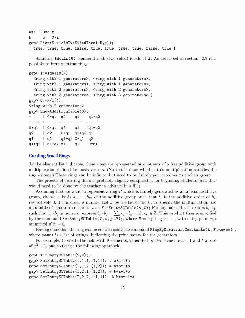
0*a | 0*a bb | b 0*agap> List(S,x->IsTwoSidedIdeal(R,x));[ true, true, true, false, true, true, true, true, false, true ]
Similarly Ideals(R ) enumerates all (two-sided) ideals of R . As described in section 2.9 it ispossible to form quotient rings.
gap> I:=Ideals(R);[ <ring with 1 generators>, <ring with 1 generators>,<ring with 1 generators>, <ring with 1 generators>,<ring with 2 generators>, <ring with 2 generators>,<ring with 2 generators>, <ring with 3 generators> ]
gap> Q:=R/I[4];<ring with 2 generators>gap> ShowAdditionTable(Q);+ | 0*q1 q2 q1 q1+q2------+------------------------0*q1 | 0*q1 q2 q1 q1+q2q2 | q2 0*q1 q1+q2 q1q1 | q1 q1+q2 0*q1 q2q1+q2 | q1+q2 q1 q2 0*q1
Creating Small Rings
As the element list indicates, these rings are represented as quotients of a free additive group withmultiplication defined for basis vectors. (No test is done whether this multiplication satisfies thering axioms.) These rings can be infinite, but need to be finitely generated as an abelian group.
The process of creating them is probably slightly complicated for beginning students (and thuswould need to be done by the teacher in advance in a file).
Assuming that we want to represent a ring R which is finitely generated as an abelian additivegroup, choose a basis b1, . . . , bm of the additive group such that li is the additive order of bi,respectively 0, if this order is infinite. Let L be the list of the li. To specify the multiplication, setup a table of structure constants with T :=EmptySCTable(m ,0); For any pair of basis vectors bi, bj ,such that bi · bj is nonzero, express bi · bj =
∑k ck · bk with ck ∈ Z. This product then is specified
by the command SetEntrySCTable(T ,i ,j ,P );, where P = [c1, 1, c2, 2, . . .], with entry pairs ci, iommitted if ci = 0.
Having done this, the ring can be created using the command RingByStructureConstants(L ,T ,names );,where names is a list of strings, indicating the print names for the generators.
For example, to create the field with 9 elements, generated by two elements a = 1 and b a rootof x2 + 1, one could use the following approach:
gap> T:=EmptySCTable(2,0);;gap> SetEntrySCTable(T,1,1,[1,1]); # a*a=1*agap> SetEntrySCTable(T,1,2,[1,2]); # a*b=1*bgap> SetEntrySCTable(T,2,1,[1,2]); # b*a=1*bgap> SetEntrySCTable(T,2,2,[-1,1]); # b*b=-1*a
45

gap> R:=RingByStructureConstants([3,3],T,["a","b"]);gap> ShowAdditionTable(R);+ | 0*a b -b a a+b a-b -a -a+b -a-b-----+---------------------------------------------0*a | 0*a b -b a a+b a-b -a -a+b -a-bb | b -b 0*a a+b a-b a -a+b -a-b -a-b | -b 0*a b a-b a a+b -a-b -a -a+ba | a a+b a-b -a -a+b -a-b 0*a b -ba+b | a+b a-b a -a+b -a-b -a b -b 0*aa-b | a-b a a+b -a-b -a -a+b -b 0*a b-a | -a -a+b -a-b 0*a b -b a a+b a-b-a+b | -a+b -a-b -a b -b 0*a a+b a-b a-a-b | -a-b -a -a+b -b 0*a b a-b a a+b
gap> ShowMultiplicationTable(R);* | 0*a b -b a a+b a-b -a -a+b -a-b-----+---------------------------------------------0*a | 0*a 0*a 0*a 0*a 0*a 0*a 0*a 0*a 0*ab | 0*a -a a b -a+b a+b -b -a-b a-b-b | 0*a a -a -b a-b -a-b b a+b -a+ba | 0*a b -b a a+b a-b -a -a+b -a-ba+b | 0*a -a+b a-b a+b -b -a -a-b a ba-b | 0*a a+b -a-b a-b -a b -a+b -b a-a | 0*a -b b -a -a-b -a+b a a-b a+b-a+b | 0*a -a-b a+b -a+b a -b a-b b -a-a-b | 0*a a-b -a+b -a-b b a a+b -a -b
Similarly, for creating (rational) quaternions with basis e, i, j, k, the following commands couldbe used:
gap> T:=EmptySCTable(4,0);;gap> SetEntrySCTable(T,1,1,[1,1]); # e*e=egap> SetEntrySCTable(T,1,2,[1,2]); # e*i=igap> SetEntrySCTable(T,1,3,[1,3]); # e*j=jgap> SetEntrySCTable(T,1,4,[1,4]); # e*k=kgap> SetEntrySCTable(T,2,1,[1,2]); # i*e=igap> SetEntrySCTable(T,2,2,[-1,1]); # i*i=-egap> SetEntrySCTable(T,2,3,[1,4]); # i*j=kgap> SetEntrySCTable(T,2,4,[-1,3]); # i*k=-jgap> SetEntrySCTable(T,3,1,[1,3]); # j*e=jgap> SetEntrySCTable(T,3,2,[-1,4]); # j*i=-kgap> SetEntrySCTable(T,3,3,[-1,1]); # j*j=-1gap> SetEntrySCTable(T,3,4,[1,2]); # j*k=igap> SetEntrySCTable(T,4,1,[1,4]); # k*e=kgap> SetEntrySCTable(T,4,2,[1,3]); # k*i=jgap> SetEntrySCTable(T,4,3,[-1,2]); # k*j=-igap> SetEntrySCTable(T,4,4,[-1,1]); # k*k=-1
46
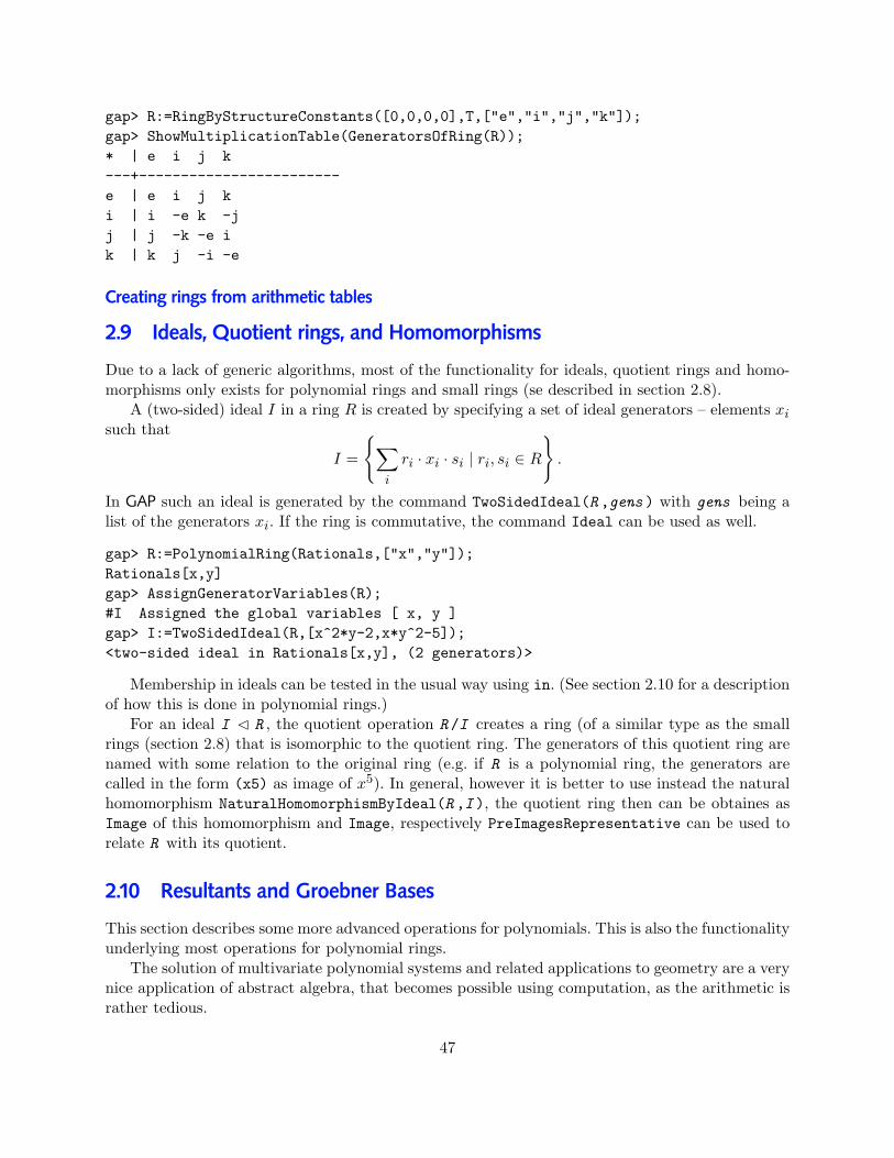
gap> R:=RingByStructureConstants([0,0,0,0],T,["e","i","j","k"]);gap> ShowMultiplicationTable(GeneratorsOfRing(R));* | e i j k---+------------------------e | e i j ki | i -e k -jj | j -k -e ik | k j -i -e
Creating rings from arithmetic tables
2.9 Ideals, Quotient rings, and Homomorphisms
Due to a lack of generic algorithms, most of the functionality for ideals, quotient rings and homo-morphisms only exists for polynomial rings and small rings (se described in section 2.8).
A (two-sided) ideal I in a ring R is created by specifying a set of ideal generators – elements xisuch that
I =
∑i
ri · xi · si | ri, si ∈ R
.
In GAP such an ideal is generated by the command TwoSidedIdeal(R ,gens ) with gens being alist of the generators xi. If the ring is commutative, the command Ideal can be used as well.
gap> R:=PolynomialRing(Rationals,["x","y"]);Rationals[x,y]gap> AssignGeneratorVariables(R);#I Assigned the global variables [ x, y ]gap> I:=TwoSidedIdeal(R,[x^2*y-2,x*y^2-5]);<two-sided ideal in Rationals[x,y], (2 generators)>
Membership in ideals can be tested in the usual way using in. (See section 2.10 for a descriptionof how this is done in polynomial rings.)
For an ideal I C R , the quotient operation R /I creates a ring (of a similar type as the smallrings (section 2.8) that is isomorphic to the quotient ring. The generators of this quotient ring arenamed with some relation to the original ring (e.g. if R is a polynomial ring, the generators arecalled in the form (x5) as image of x5). In general, however it is better to use instead the naturalhomomorphism NaturalHomomorphismByIdeal(R ,I ), the quotient ring then can be obtaines asImage of this homomorphism and Image, respectively PreImagesRepresentative can be used torelate R with its quotient.
2.10 Resultants and Groebner Bases
This section describes some more advanced operations for polynomials. This is also the functionalityunderlying most operations for polynomial rings.
The solution of multivariate polynomial systems and related applications to geometry are a verynice application of abstract algebra, that becomes possible using computation, as the arithmetic israther tedious.
47
Resultants are one of the topics that vanished from the standard syllabus with the rise of modernalgebra. Nevertheless they can be very useful for obtaining concrete results. A description suitablefor undergraduate courses can be found for example in [CLO07, section XXX].
The two fundamental properties of the resultant r(y) := resx(f(x, y), g(x, y)) (where y in factcould be a set of variables) are:
Variable elimination If (x, y) is a common zero for f and g, then y is a zero for r(y). Thus onecan often solve systems of polynomial equations in a process similar to Gaussian elimination,using resultants for variable elimination. Note that resultants can turn out to be zero andthat the order of elimination is often crucial.
Root arithmetic If f, g ∈ F [x] and α, β in the splitting field of f and g such that f(α) andg(β) = 0, then
resy(f(x− y), g(y)) has root α+ βresy(yn · f(x/y), g(y)) has root α · β
This allows to construct polynomials with more complicated roots, and – via the primitive elementtheorem – polynomials with bespoke, more complicated splitting fields, see chapter ??.
Resultants in GAP are rather straightforward. The syntax is Resultant(pol1,pol2,elimvar ),the result is a polynomial with the specified variable eliminated.
gap> f:=x^2-3;x^2-3gap> g:=x^2-5;x^2-5gap> r:=Resultant(Value(f,x-y),Value(g,y),y);x^4-16*x^2+4gap> Value(r,Sqrt(3)+Sqrt(5)); # as described above uner root arithmetic0
There is no functionality that will automatically form iterated resultants. Also, as soon as rootsget beyond quadratic irrationalities, it can be hard if not impossible to find and express root valuesfor back substitution. Exercise 15 illustrates the process.
Groebner Bases Groebner bases are the fundamental tool for calculations in multivariate poly-nomial rings. In recent years this topic has started to move into textbooks. Again, besides strength-ening the concept of ideals and factor ring elements, they allow for a series of interesting applications:
Solving Polynomial Systems Groebner bases with respect to a lexicographic ordering offer im-mediately a “triangulization” as desired for solving a system of polynomial equations.
Canonical representatives for quotient rings In the same way that the remainder of poly-nomial division can be used to describe the quotient ring of a univariate polynomial ring,reduction using a degree ordering allows for a description of canonical representatives forR/I and thus a description of R/I. This is a good way of constructing rings with bespokeproperties.
48

Geometry Besides being a main tool for algebraic geometry, Groebner bases can be used to de-scribe situations in Euclidean geometry via polynomials in the coordinates, and subsequentlyto construct “arithmetic” proofs for problems from classical geometry. This setup also leadseasily to the impossibility of many classical problems using field extensions.
The handout 2.11 introduces the treatment geometric problems using polynomials and ad-dresses Groebner basis issues, including the question of constants versus variables.
Underlying a Groebner basis calculation is the definition of a suitable ordering. Orderings in GAPare created by functions, which can take a sequence of indeterminates (either multiple arguments ora list) as arguments. In this case these indeterminates are ordered as given. Indeterminates that arenot given have lower rank and are ordered according to their internal index number. (For furtherdetails on orderings, see the system manual.)
GAP provides the following polynomial orderings:
MonomialLexOrdering() implements a lexicographic (lex) ordering, i.e. monomials are comparedby the exponent vectors as words in the dictionary. The default monomial ordering simplyorders the indeterminates by their index number, i.e. x1 > x2 > · · · . A lexicographic orderingis required for solving polynomial systems.
MonomialLexOrdering(x,y,z) implements a lex ordering with x > y > z. If the indeterminateswere defined in the natural order, this is exactly the same as MonomialLexOrdering().
MonomialGrlexOrdering() implements a grlex ordering which compares first by total degreeand the lexicographically. Again it is possible to indicate a variable ordering.
MonomialGrevlexOrdering() implements a grevlex ordering which first compares by degree andthen reverse lexicographic. Often this is the most efficient ordering for computing a Gr”oebnerbasis.
LeadingTermOfPolynomial(pol,ordering ) returns the leading term of the polynomial pol ,LeadingCoefficientOfPolynomial(pol,ordering ) and LeadingMonomialOfPolynomial(pol,ordering )respectively its coefficient and monomial factors.
gap> x:=X(Rationals,"x");;y:=X(Rationals,"y");;z:=X(Rationals,"z");;gap> lexord:=MonomialLexOrdering();grlexord:=MonomialGrlexOrdering();MonomialLexOrdering()MonomialGrlexOrdering()gap> f:=2*x+3*y+4*z+5*x^2-6*z^2+7*y^3;;gap> LeadingMonomialOfPolynomial(f,grlexord);y^3gap> LeadingTermOfPolynomial(f,lexord);5*x^2gap> LeadingMonomialOfPolynomial(f,lexord);x^2gap> LeadingTermOfPolynomial(f,MonomialLexOrdering(z,y,x));-6*z^2gap> LeadingTermOfPolynomial(f,MonomialLexOrdering(y,z,x));7*y^3
49

gap> LeadingTermOfPolynomial(f,grlexord);7*y^3gap> LeadingCoefficientOfPolynomial(f,lexord);5gap> l:=[f,Derivative(f,x),Derivative(f,y),Derivative(f,z)];;gap> Sort(l,MonomialComparisonFunction(lexord));l;[ -12*z+4, 21*y^2+3, 10*x+2, 7*y^3+5*x^2-6*z^2+2*x+3*y+4*z ]gap> Sort(l,MonomialComparisonFunction(MonomialLexOrdering(z,y,x)));l;[ 10*x+2, 21*y^2+3, -12*z+4, 7*y^3+5*x^2-6*z^2+2*x+3*y+4*z ]
A Groebner basis in GAP is simply a list of polynomials, and is computed from a list of poly-nomials with respect to a supplied ordering and is computed from a list pols of polynomialsvia GroebnerBasis(pols,ordering ). The algorithm used is a rather straightforward implemen-tation of Buchberger’s algorithm which should be sufficient for teaching purposes but will not becompetitive with dedicated systems.
There also is ReducedGroebnerBasis(pols,ordering ), which removes redundancies from theresulting list and scales the leading coefficient to 1. (The resulting basis is unique for the ideal.)For all practical applications this is preferrable to the ordinary GroebnerBasis command, whichis provided purely for illustrating the process of computing such a basis.
gap> l:=[x^2+y^2+z^2-1,x^2+z^2-y,x-y];;gap> GroebnerBasis(l,MonomialLexOrdering());[ x^2+y^2+z^2-1, x^2+z^2-y, x-y, -y^2-y+1, -z^2+2*y-1, 1/2*z^4+2*z^2-1/2 ]gap> GroebnerBasis(l,MonomialLexOrdering(z,y,x));[ x^2+y^2+z^2-1, x^2+z^2-y, x-y, -x^2-x+1 ]gap> ReducedGroebnerBasis(l,MonomialLexOrdering());[ z^4+4*z^2-1, -1/2*z^2+y-1/2, -1/2*z^2+x-1/2 ]gap> ReducedGroebnerBasis(l,MonomialLexOrdering(z,y,x));[ x^2+x-1, -x+y, z^2-2*x+1 ]
Issuing the command SetInfoLevel(InfoGroebner,3); prompts GAP to print informationabout the progress of the calculation, including the S-polynomials computed.
gap> SetInfoLevel(InfoGroebner,3);gap> bas:=GroebnerBasis(l,MonomialLexOrdering());#I Spol(2,1)=-y^2-y+1#I reduces to -y^2-y+1#I |bas|=4, 7 pairs left#I Spol(3,1)=-x*y-y^2-z^2+1#I reduces to -z^2+2*y-1#I |bas|=5, 11 pairs left#I Pair (3,2) avoided#I Pair (4,1) avoided#I Pair (4,2) avoided#I Pair (4,3) avoided#I Spol(4,4)=0#I Pair (5,1) avoided
50

#I Pair (5,2) avoided#I Pair (5,3) avoided#I Spol(5,4)=y*z^2+3*y-2#I reduces to 1/2*z^4+2*z^2-1/2#I |bas|=6, 8 pairs left#I Spol(5,5)=0#I Pair (6,1) avoided#I Pair (6,2) avoided#I Pair (6,3) avoided#I Pair (6,4) avoided#I Pair (6,5) avoided#I Spol(6,6)=0[ x^2+y^2+z^2-1, x^2+z^2-y, x-y, -y^2-y+1, -z^2+2*y-1, 1/2*z^4+2*z^2-1/2 ]
For a known Groebner basis , the command PolynomialReduction(poly,basis,ordering )reduces poly with respect to basis . It returns a list [remainder,quotients ] where poly =∑i quotients i ·basis i+remainder . (Note that the reduction process used differs from textbook
formulations, the “textbook” version is implemented via PolynomialDivisionAlgorithm(poly,basis,ordering ).)Similarly PolynomialReducedRemainder(poly,basis,ordering ) returns only the remainder .
gap> PolynomialReduction(2*(x*y*z)^2,bas,MonomialLexOrdering());[ 13*z^2-3,[ 2*y^2*z^2, 0, 0, 2*y^2*z^2+2*z^4-2*y*z^2+2*z^2, z^4+2*z^2, 2*z^2-6 ] ]
gap> PolynomialDivisionAlgorithm(2*(x*y*z)^2,bas,MonomialLexOrdering());[ 13*z^2-3,[ 2*y^2*z^2, 0, 0, 2*y^2*z^2+2*z^4-2*y*z^2+2*z^2, z^4+2*z^2, 2*z^2-6 ] ]
gap> PolynomialReducedRemainder(2*(x*y*z)^2,bas,MonomialLexOrdering());13*z^2-3
2.11 Handouts
Some aspects of Grobner bases
Constants Sometimes we want to solve a Grobner basis for situations where there are constantsinvolved. We cannot simply consider these constants as further variables (e.g. one cannot solve forthese.) Instead, suppose that we have constants c1, . . . , ck and variables x1, . . . , xn.
We first form the polynomial ring in the constants, C := k[c1, . . . , ck]. This is an integraldomain, we therefore (Theorem 2.25 in the book) can from the field of fractions (analogous to howthe rationals are formed as fractions of integers) F = Frac(C) = k(c1, . . . , ck)2.
We then set R = F [x1, . . . , xn] = k(c1, . . . , ck)[x1, . . . , xn] and work in this polynomial ring.(The only difficulty arises once one specializes the constants: It is possible that denominatorsevaluate back to zero.)
For example, suppose we want to solve the equations
x2y + y + a = y2x+ x = 0
2The round parentheses denote that we permit also division
51
In GAP we first create the polynomial ring for the constants:
gap> C:=PolynomialRing(Rationals,["a"]);Rationals[a]gap> a:=IndeterminatesOfPolynomialRing(S)[1];a
(There is no need to create a separate fraction field. Now we define the new variables x, y to havecoefficients from C:
gap> x:=X(C,"x");;#I You are creating a polynomial *over* a polynomial ring (i.e. in an#I iterated polynomial ring). Are you sure you want to do this?#I If not, the first argument should be the base ring, not a polynomial ring#I Set ITER_POLY_WARN:=false; to remove this warning.gap> y:=X(C,"y");;
As one sees, GAP warns that these variables are defined over a ring which has already variables,but we can ignore this warning3, or set ITER_POLY_WARN:=false; to turn it off.
Now we can form polynomials and calculate a Grobner basis:
gap> f:=x^2*y+y+a;;gap> g:=y^2*x+x;;gap> ReducedGroebnerBasis([f,g],MonomialLexOrdering());[ y^3+a*y^2+y+a, x*y^2+x, x^2-y^2-a*y ]
We thus need that y3 + ay2 + y + a = 0, and then can solve this for y and substitute back.
The Nullstellensatz and the Radical In applications (see below) we sometimes want to checknot whether g ∈ I C R, but whether g has “the same roots” as I. (I.e. we want that g(x1, . . . , xn) =0 if and only if f(x1, . . . , xn) = 0 for all f ∈ I.) Clearly this can hold for polynomials not in I, forexample consider I =
⟨x2⟩
C Q[x], then g(x) = x 6∈ I, but has the same roots.An important theorem from algebraic geometry show that over C, such a power condition is all
that can happen4:
Theorem (Hilbert’s Nullstellensatz): Let R = C[x1, . . . , xn] and I C R. If g ∈ Rsuch that g(x1, . . . , xn) = 0 if and only if f(x1, . . . , xn) = 0 for all f ∈ I, then thereexists an integer m, such that gm ∈ I.
The set g ∈ R | ∃m : gm ∈ I is called the Radical of I.There is a neat way how one can test this property, without having to try out possible m:
Suppose R = k[x1, . . . , xn] and I = 〈f1, . . . , fm〉 C R. Let g ∈ R. Then there exists a naturalnumber m such that gm ∈ I if and only if (we introduce an auxiliary variable y)
1 ∈ 〈f1, . . . , fm, 1− yg〉 =: I C k[x1, . . . , xn, y]
3The reason for the warning is that this was a frequent error of users when defining variables and polynomialrings. Variables were taken accidentally not from the polynomial ring, but created over the polynomial ring.
4Actually, one does not need C, but only that the field is algebraically closed
52

The reason is easy: If 1 ∈ I, we can write
1 =∑i
p(x1, . . . , xn, y) · fi(x1, . . . , xn) + q(x1, . . . , xn, y) · (1− yg)
We now set y = 1/g (formally in the fraction field) and multiply with a sufficient high power(exponent m) of g, to clean out all g in the denominators. We obtain
gm =∑i
gm · p(x1, . . . , xn, 1/gm)︸ ︷︷ ︸∈R
·fi(x1, . . . , xn) + gm · q(x1, . . . , xn, y) · (1− y/y)︸ ︷︷ ︸=0
∈ I.
Vice versa, if gm ∈ I, then
1 = ymgm + (1− ymgm) = ymgm︸ ︷︷ ︸∈I⊂I
+ (1− yg)︸ ︷︷ ︸∈I
(1 + yg + · · ·+ ym−1gm−1) ∈ I
This property can be tested easily, as 1 ∈ I ⇔ I = k[x1, . . . , xn, y], which is the case only if aGrobner basis for I contains a constant.
We will see an application of this below.
Proving Theorems from Geometry Suppose we describe points in the plane by their (x, y)-coordinates. We then can describe many geometric properties by polynomial equations:
Theorem: Suppose that A = (xa, ya), B = (xb, yb), C = (xc, yc) and D = (xd, yd) are pointsin the plane. Then the following geometric properties are described by polynomial equations:
AB is parallel to CD:yb − yaxb − xa
=yd − ycxd − xc
, which implies (yb−ya)(xd−xc) = (yd−yc)(xb−xa).
AB ⊥ CD: (xb − xa)(xd − xc) + (yb − ya)(yd − yc) = 0.
|AB| = |CD|: (xb − xa)2 + (yb − ya)2 = (xd − xc)2 + (yd − yc)2.
C lies on the circle with center A though the point B: |AC| = |AB|.
C is the midpoint of AB: xc =12
(xb − xa), yc = 12(yb = ya).
C is collinear with AB: self
BD bisects ∠ABC: self
A theorem from geometry now sets up as prerequisites some points (and their relation withcircles and lines) and claims (the conclusion) that this setup implies other conditions. If we supposethat (xi, yi) are the coordinates of all the points involved, the prerequisites thus are described bya set of polynomials fj ∈ Q[x1, . . . , xn, y1, . . . , yn] =: R. A conclusion similarly corresponds to apolynomials g ∈ R.
The statement of the geometric theorem now says that whenever the (xi, yi) are points ful-filling the prerequisites (i.e. fj(x1, . . . , xn, y1, . . . , yn) = 0), then also the conclusion holds for thesepoints (i.e. g(x1, . . . , xn, y1, . . . , yn) = 0).
This is exactly the condition we studied in the previous section and translated to gm ∈〈f1, . . . , fm〉, which we can test.
53
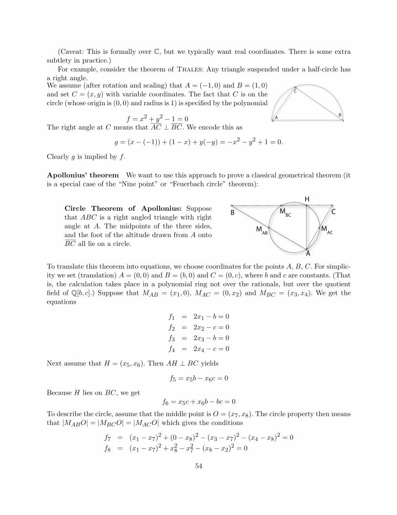
(Caveat: This is formally over C, but we typically want real coordinates. There is some extrasubtlety in practice.)
For example, consider the theorem of Thales: Any triangle suspended under a half-circle hasa right angle.We assume (after rotation and scaling) that A = (−1, 0) and B = (1, 0)and set C = (x, y) with variable coordinates. The fact that C is on thecircle (whose origin is (0, 0) and radius is 1) is specified by the polynomial
f = x2 + y2 − 1 = 0 A
C
B
The right angle at C means that AC ⊥ BC. We encode this as
g = (x− (−1)) + (1− x) + y(−y) = −x2 − y2 + 1 = 0.
Clearly g is implied by f .
Apollonius’ theorem We want to use this approach to prove a classical geometrical theorem (itis a special case of the “Nine point” or “Feuerbach circle” theorem):
Circle Theorem of Apollonius: Supposethat ABC is a right angled triangle with rightangle at A. The midpoints of the three sides,and the foot of the altitude drawn from A ontoBC all lie on a circle.
A
B C
H
MBC
MACM
AB
To translate this theorem into equations, we choose coordinates for the points A, B, C. For simplic-ity we set (translation) A = (0, 0) and B = (b, 0) and C = (0, c), where b and c are constants. (Thatis, the calculation takes place in a polynomial ring not over the rationals, but over the quotientfield of Q[b, c].) Suppose that MAB = (x1, 0), MAC = (0, x2) and MBC = (x3, x4). We get theequations
f1 = 2x1 − b = 0f2 = 2x2 − c = 0f3 = 2x3 − b = 0f4 = 2x4 − c = 0
Next assume that H = (x5, x6). Then AH ⊥ BC yields
f5 = x5b− x6c = 0
Because H lies on BC, we getf6 = x5c+ x6b− bc = 0
To describe the circle, assume that the middle point is O = (x7, x8). The circle property then meansthat |MABO| = |MBCO| = |MACO| which gives the conditions
f7 = (x1 − x7)2 + (0− x8)2 − (x3 − x7)2 − (x4 − x8)2 = 0f8 = (x1 − x7)2 + x2
8 − x27 − (x8 − x2)2 = 0
54
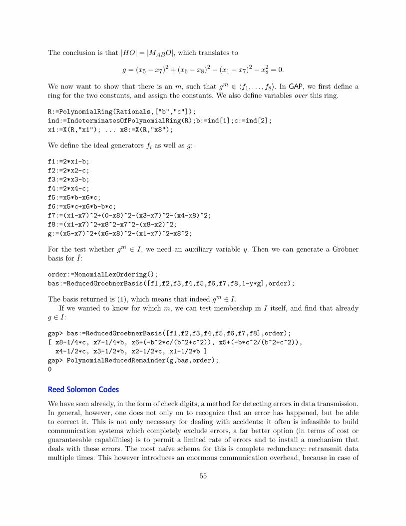
The conclusion is that |HO| = |MABO|, which translates to
g = (x5 − x7)2 + (x6 − x8)2 − (x1 − x7)2 − x28 = 0.
We now want to show that there is an m, such that gm ∈ 〈f1, . . . , f8〉. In GAP, we first define aring for the two constants, and assign the constants. We also define variables over this ring.
R:=PolynomialRing(Rationals,["b","c"]);ind:=IndeterminatesOfPolynomialRing(R);b:=ind[1];c:=ind[2];x1:=X(R,"x1"); ... x8:=X(R,"x8");
We define the ideal generators fi as well as g:
f1:=2*x1-b;f2:=2*x2-c;f3:=2*x3-b;f4:=2*x4-c;f5:=x5*b-x6*c;f6:=x5*c+x6*b-b*c;f7:=(x1-x7)^2+(0-x8)^2-(x3-x7)^2-(x4-x8)^2;f8:=(x1-x7)^2+x8^2-x7^2-(x8-x2)^2;g:=(x5-x7)^2+(x6-x8)^2-(x1-x7)^2-x8^2;
For the test whether gm ∈ I, we need an auxiliary variable y. Then we can generate a Grobnerbasis for I:
order:=MonomialLexOrdering();bas:=ReducedGroebnerBasis([f1,f2,f3,f4,f5,f6,f7,f8,1-y*g],order);
The basis returned is (1), which means that indeed gm ∈ I.If we wanted to know for which m, we can test membership in I itself, and find that already
g ∈ I:
gap> bas:=ReducedGroebnerBasis([f1,f2,f3,f4,f5,f6,f7,f8],order);[ x8-1/4*c, x7-1/4*b, x6+(-b^2*c/(b^2+c^2)), x5+(-b*c^2/(b^2+c^2)),x4-1/2*c, x3-1/2*b, x2-1/2*c, x1-1/2*b ]
gap> PolynomialReducedRemainder(g,bas,order);0
Reed Solomon Codes
We have seen already, in the form of check digits, a method for detecting errors in data transmission.In general, however, one does not only on to recognize that an error has happened, but be ableto correct it. This is not only necessary for dealing with accidents; it often is infeasible to buildcommunication systems which completely exclude errors, a far better option (in terms of cost orguaranteeable capabilities) is to permit a limited rate of errors and to install a mechanism thatdeals with these errors. The most naıve schema for this is complete redundancy: retransmit datamultiple times. This however introduces an enormous communication overhead, because in case of
55
a single retransmission it still might not be possible to determine which of two different values iscorrect. In fact we can guarantee a better error correction with less overhead, as we will see below.
The two fundamental problems in coding theory are:
Theory: Find good (i.e. high error correction at low redundancy) codes.
Practice: Find efficient ways to implement encoding (assigning messages to code words) anddecoding (determining the message from a possibly distorted code word).
In theory, almost (up to ε) optimal encoding can be achieved by choosing essentially random codegenerators, but then decoding can only be done by table lookup. To use the code in practice thereneeds to be some underlying regularity of the code, which will enable the algorithmic encoding anddecoding. This is where algebra comes in.
A typical example of such a situation is the compact disc: not only should this system beimpervious to fingerprints or small amounts of dust. At the time of system design (the late 1970s)it actually was not possible to mass manufacture compact discs without errors at any reasonableprice. The design instead assumes errors and includes capability for error correction. It is importantto note that we really want to correct all errors (this would be needed for a data CD) and notjust conceal errors by interpolating erroneous data (which can be used with music CDs, thougheven music CDs contain error correction to deal with media corruption). This extra level of errorcorrection can be seen in the fact that a data CD has a capacity of 650 MB, while 80 minutes ofmusic in stereo, sampled at 44,100 Hz, with 16 bit actually amount to 80 · 60 · 2 · 44100 · 2 bytes =846720000 bytes = 808MB5, the overhead is extra error correction on a data CD.
The first step towards error correction is interleaving. As errors are likely to occur in bursts ofphysically adjacent data (the same holds for radio communication with a spaceship which might getdisturbed by cosmic radiation) subsequent data ABCDEF is actually transmitted in the sequenceADBECF. An error burst – say erasing C and D – then is spread over a wider area AXBEXF whichreduces the local error density. We therefore can assume that errors occur randomly distributedwith bounded error rate.
The rest of this document now describes the mathematics of the system which is used for errorcorrection on a CD (so-called Reed-Solomon codes) though for simplicity we will choose smallerexamples than the actual codes being used.
We assume that the data comes in the form of elements of a field F .The basic idea behind linear codes is to choose a sequence of code generators g1, . . . , gk each
of length > k and to replace a sequence of k data elements a1, . . . , ak by the linear combinationa1g1 + a2g2 + · · ·+ akgk, which is a slightly longer sequence. This longer sequence (the code word)is transmitted. We define the code to be the set of all possible code words.
For example (assuming the field with 2 elements) if the gi are given by the rows of the generator
matrix
1 0 0 1 0 00 1 0 0 1 00 0 1 0 0 1
we would replace the sequence a, b, c by a, b, c, a, b, c, while (a code
with far better error correction!) the matrix
1 0 1 0 1 0 10 1 1 0 0 1 10 0 0 1 1 1 1
would have us replace a, b, c
bya, b, a+ b, c, a+ c, b+ c, a+ b+ c.
51MB is 10242 bytes
56

We notice in this example that there are 23 = 8 combinations, any two of which differ in at least3 places. If we receive a sequence of 7 symbols with at most one error therein, we can thereforedetermine in which place the error occurred and thus can correct it. We thus have an 1-errorcorrecting code.
Next we want to assume (regularity!) that any cyclic shift of a code word is again a code word.We call such codes cyclic codes. It now is convenient to represent a code word c0, . . . , cn−1 by thepolynomial c0 +c1x+c2x2 + · · ·+cn−1x
n−16. A cyclic shift now means to multiply by x, identifyingxn with x0 = 1. The transmitted messages therefore are not really elements of the polynomial ringF [x], but elements of the factor ring F [x]/I with I = 〈xn − 1〉 C F [x]. The linear process of addingup generators guarantees that the sum or difference of code words is again a code word. A cyclicshift of a code word I + w then corresponds to the product (I + w) · (I + x). As any element ofF [x]/I is of the form I + p(x), demanding that cyclic shifts of code words are again code wordsthus implies that the product of any code word (I + w) with any factor element (I + r) is againa code word. We thus see that the code (i.e. the set of possible messages) is an ideal in F [x]/I.We have seen in homework problem 38 that any such ideal — and thus any cyclic code – must beof the form 〈I + d〉 with d a divisor of xn − 1. If d = d0 + d1x + · · · + dsx
s, we get in the abovenotation the generator matrix
d0 d1 · · · ds 0 0 · · · 00 d0 d1 · · · ds 0 · · · 00 0 d0 d1 · · · ds · · · 0
...0 0 · · · 0 d0 d1 · · · ds
.
As d is a divisor of xn− 1 any further cyclic shift of the last generator can be expressed in terms ofthe other generators. One can imagine the encoding process as evaluation of a polynomial at morepoints than required for interpolation. This makes it intuitively clear that it is possible to recoverthe correct result if few errors occur. The more points we evaluate at, the better error correctionwe get (but also the longer the encoded message gets).
The task of constructing cyclic codes therefore has been reduced to the task of finding suitable(i.e. guaranteeing good error correction and efficient encoding and decoding) polynomials d.
The most important class of cyclic codes are BCH-codes which are defined by prescribing thezeroes of d. One can show that a particular regularity of these zeroes produces good error correction.Reed-Solomon Codes (as used for example on a CD) are an important subclass of these codes.
To define such a code we start by picking a field with q elements. Such fields exists for any primepower q = pm and can be constructed as quotient ring Zp[x]/ 〈p(x)〉 for p an irreducible polynomialof degree m. (Using fields larger than Zp is crucial for the mechanism.) The code words of the codewill have length q − 1. If we have digital data it often is easiest to simply bundle by bytes and touse a field with q = 28 = 256 elements.
We also choose the number s < q−12 of errors per transmission unit of q − 1 symbols which
we want to be able to correct. This is a trade-off between transmission overhead and correctioncapabilities, a typical value is s = 2.
It is known that in any finite field there is a particular element α (a primitive root), such thatαq−1 = 1 but αk 6= 1 for any k < q − 1. (This implies that all powers αk (k < q − 1) are different.
6Careful: We might represent elements of F also by polynomials. Do not confuse these polynomials with the codepolynomials
57

Therefore every nonzero element in the field can be written as a power of α.) As every power β = αk
also fulfills that βq−1 = 1 we can conclude that
xq−1 − 1 =q−1∏k=0
(x− αk).
The polynomial d(x) = (x− α)(x− α2)(x− α3) · · · (x− α2s) therefore is a divisor of xq−1 − 1 andtherefore generates a cyclic code. This is the polynomial we use. The dimension (i.e. the minimalnumber of generators) of the code then is q − 1 − 2s, respectively 2s symbols are added to everyq − 1− 2s data symbols for error correction.
For example, take q = 8. We take the field with 8 elements as defined in GAP via the polynomialx3 + x + 1, the element α is represented by Z(8). We also choose s = 1. The polynomial definingthe code is therefore d = (x− α)(x− α2).
gap> x:=X(GF(8),"x");;gap> alpha:=Z(8);Z(2^3)gap> d:=(x-alpha)*(x-alpha^2);x^2+Z(2^3)^4*x+Z(2^3)^3
We build the generator matrix from the coefficients of the polynomial:
gap> coe:=CoefficientsOfUnivariatePolynomial(d);[ Z(2^3)^3, Z(2^3)^4, Z(2)^0 ]gap> g:=NullMat(5,7,GF(8));;gap> for i in [1..5] do g[i][i..i+2]:=coe;od;Display(g);z^3 z^4 1 . . . .. z^3 z^4 1 . . . z = Z(8). . z^3 z^4 1 . .. . . z^3 z^4 1 .. . . . z^3 z^4 1
To simplify the following description we convert this matrix into RREF. (This is just a base changeon the data and does not affect any properties of the code.)
gap> TriangulizeMat(g); Display(g);1 . . . . z^3 z^4. 1 . . . 1 1 z = Z(8). . 1 . . z^3 z^5. . . 1 . z^1 z^5. . . . 1 z^1 z^4
What does this mean now: Instead of transmitting the data ABCDE we transmit ABCDEPQ withthe two error correction symbols defined by
P = α3A+B + α3C + αD + αE
Q = α4A+B + α5C + α5D + α4E
58

For decoding and error correction we want to find (a basis of) the relations that hold for all therows of this matrix. This is the nullspace7 of the matrix (and in fact is the same as if we had notRREF).
gap> h:=NullspaceMat(TransposedMat(g));;Display(h);z^3 1 z^3 z^1 z^1 1 . z = Z(8)z^4 1 z^5 z^5 z^4 . 1
When receiving a message ABCDEPQ we therefore calculate two syndromes8
S = α3A+B + α3C + αD + αE + P
T = α4A+B + α5C + α5D + α4E +Q
If no error occurred both syndromes will be zero. However now suppose an error occurred andinstead of ABCDEPQ we receive A’B’C’D’E’P’Q’ where A′ = A+EA and so on. Then we get thesyndromes
S′ = α3A′ +B′ + α3C ′ + αD′ + αE′ + P ′
= α3(A+ EA) + (B + EB) + α3(C + EC) + α(D + ED) + α(E + EE) + (P + EP )= α3A+B + α3C + αD + αE + P︸ ︷︷ ︸
= 0 by definition of the syndrome
+α3EA + EB + α3EC + αED + αEE + EP
= α3EA + EB + α3EC + αED + αEE + EP
and similarlyT ′ = α4EA + EB + α5EC + α5ED + α4EE + EQ
If symbol A’ is erroneous, we have that T ′ = αS′, the error is EA = α4S′ (using that α3 · α4 = 1).If symbol B’ is erroneous, we have that T ′ = S′, the error is EB = S′.If symbol C’ is erroneous, we have that T ′ = α2S′, the error is EC = α4S′.If symbol D’ is erroneous, we have that T ′ = α4S′, the error is ED = α6S′.If symbol E’ is erroneous, we have that T ′ = α3S′, the error is EE = α6S′.If symbol P’ is erroneous, we have that S′ 6= 0 but T ′ = 0, the error is EP = S′.If symbol Q’ is erroneous, we have that T ′ 6= 0 but S′ = 0, the error is EQ = T ′.
For an example, suppose we want to transmit the message
A = α3, B = α2, C = α, D = α4, E = α5.
We calculate
P = α3A+B + α3C + αD + αE = α6
Q = α4A+B + α5C + α5D + α4E = 0
7actually the right nullspace, which is the reason why we need to transpose in GAP, which by default takes leftnullspaces
8These syndromes are not unique. Another choice of nullspace generators would have yielded other syndromes.
59

gap> a^3*a^3+a^2+a^3*a+a*a^4+a*a^5;Z(2^3)^6gap> a^4*a^3+a^2+a^5*a+a^5*a^4+a^4*a^5;0*Z(2)
We can verify the syndromes for this message:
gap> S:=a^3*a^3+a^2+a^3*a+a*a^4+a*a^5+a^6;0*Z(2)gap> T:=a^4*a^3+a^2+a^5*a+a^5*a^4+a^4*a^5+0;0*Z(2)
Now suppose we receive the message
A = α3, B = α2, C = α, D = α3, E = α5, P = α6, Q = 0.
We calculate the syndromes as S = 1, T = a4:
gap> S:=a^3*a^3+a^2+a^3*a+a*a^3+a*a^5+a^6;Z(2)^0gap> T:=a^4*a^3+a^2+a^5*a+a^5*a^3+a^4*a^5+0;Z(2^3)^4
We recognize that T = α4S, so we see that symbol D is erroneous. The error is ED = α6S = α6
and thus the correct value for D is α3 − α6 = α4.
gap> a^3-a^6;Z(2^3)^4
It is not hard to see that if more (but not too many) than s errors occur, the syndromes stillindicate that an error happened, even though we cannot correct it any longer. (One can in factdetermine the maximum number of errors the code is guaranteed to detect, even if it cannot correctit any longer.) This is used in the CD system by combining two smaller Reed-Solomon codes in aninterleaved way. The result is called a Cross-Interleave Reed-Solomon code (CIRC): Consider themessage be placed in a grid like this:
A B C DE F G HI J K L
The first code acts on rows (i.e. ABCD, EFGH,. . . ) and corrects errors it can correct. If it detectserrors, but cannot correct them, it marks the whole row as erroneous, for example:
A B C DX X X XI J K L
The second code now works on columns (i.e. AXI, BXJ) and corrects the values in the rows markedas erroneous. (As we know which rows these are, we can still correct better than with the secondcode alone!) One can show that this combination produces better performance than a single codewith higher error correction value s.
60

2.12 Problems
Exercise 2. Compute the Gcd of a = 67458 and b = 43521 and express it in the form xa+ yb.
Exercise 3. Calculate the gcd of x4+4x3−13x2−28x+60 and x6+5x5−x4−29x3−12x2+36x.
Exercise 4. a) Determine the check-digit for the ISBN 3-86073-427-?b) Show (by giving an explicit example) that the check-digit of the ISBN does not necessarily correctmultiple errors.
Exercise 5. The easter formula of Gauß provides a way for calculating the date of easter (i.e. thefirst sunday after the first full moon of spring) in any particular year. For the period 1900-2099 (arestriction due to the use of the Georgian calendar) a simplified version is:
• Suppose the year is Y .
• Calculate a = Y mod 19, b = Y mod 4, c = Y mod 7.
• Calculate d = (19a+ 24)mod30 and e = (2b+ 4c+ 6d+ 5)mod7
• If d+ e < 10 then easter will fall on the (d+ e+ 22)th March, otherwise the (d+ e− 9)th ofApril.
• Exception: If the date calculated is April 26, then easter will be April 19 instead. (There isa further exception in western (i.e. not orthodox) churches for certain April 25 dates, againdue to the Georgian calendar, which we ignore for simplicity.)
a) Calculate the easter day for 2010 and for 1968.b) Show, by finding explicitly years for which this holds, that the date may lie on March 23. (March22 is possible but does not occur between 1900 and 2099.)c) Assuming the formula would work for any year (not just 1900-2099), what is the smallest period,after which we can guarantee that the sequence of dates repeats?
Exercise 6. Let p(x) = x3− 6x2 + 12x− 3 and α ∈ R a root of p(x). (Calculus shows there is onlyone real root.)a) Let f(x) ∈ Q[x] be any rational polynomial and g(x) = f(x) mod p(x). Show that f(α) = g(α).Note: We can therefore calculate with polynomials modulo p(x) and have x play the role of α –for example when calculating α5 we note that x5 mod p(x) = 75x2 − 270x + 72, therefore α5 =75α2 − 270α+ 72.b) Calculate (x− 2)3 mod p. What can you conclude from this about α?
Exercise 7. In this problem we are working modulo 3. Consider the polynomial f(x) = x2 − 2.a) Determine the nine possible remainders when dividing any polynomial by f modulo 3.b) Let R be the set of these remainders with addition and multiplication modulo f and modulo 3.Construct the addition and multiplication table.c) Show that the polynomials of degree zero create a subring. We can identify this subring with Z3.d) Show that the equation y2 + 1 = 0 has no solution in Z3.
61

e) Show that the equation y2 + 1 = 0 has a solution in R. (We therefore could consider R as Z3[i].)f) Show that every nonzero element of R has a multiplicative inverse.
Exercise 8. Let F = Z2 be the field with two elements. Show that the rings (actually, both arefields – you don’t need to show this) F[x]/
⟨x3 + x+ 1
⟩and F[x]/
⟨x3 + x2 + 1
⟩are isomorphic.
Hint: In the second ring, find an element α such that α3+α+1 = 0 and use this to find how to mapI +x from the first ring. Then extend in the obvious way to the whole ring. You are not required tocheck that the whole addition/multiplication tables are mapped to each other (which would be rathertedious), just test a handful of cases.
Exercise 9. Let R = Z[i] =a+ b
√−1 | a, b ∈ Z
. We define d(a+bi) := (a+bi)·(a+ bi) = a2+b2.
a) Show: For x, y ∈ R there are q, r ∈ R such that x = qy + r with r = 0 or d(r) < d(y), i.e. Ris a euclidean ring. (Hint: Consider R as points in the complex plane and for a, b ∈ R chooseq := m+ ni ∈ R such that |a/b− (m+ ni)| ≤ 1/
√2.)
b) Determine the gcd of 7 + i and −1 + 5i.(If you want to do complex arithmetic in GAP, you can write E(4) to represent i.)Exercise 10.
Exercise 11. Show that the following polynomials ∈ Z[x] are irreducible, by considering theirreductions modulo primes.
1. x5 + 5x2 − 1
2. x4 + 4x3 + 6x2 + 4x− 4
3. x7 − 30x5 + 10x2 − 120x+ 60
Exercise 12. The following polynomials are irreducible (i.e. have no proper factors of degree ≥ 1)over the field Z2:
x2 + x+ 1, x3 + x+ 1, x4 + x+ 1
The corresponding quotient rings Q := Z2[x]/ 〈p(x)〉 therefore are fields (with respectively 4,8 and16 elements). For each of these fields Q (with 2n elements) show (by trying out multiplicationof elements in Q) that there is an element α ∈ Q such that α2n−1 = 1 but αm 6= 1 for all0 < m < nn − 1. (Such an element α is called a primitive root. All finite fields have primitiveroots, which will be shown in a more advanced course. Primitive roots are important in manyapplications. When creating finite fields in GAP, it actually represents all nonzero elements aspowers of a primitive root. See for example the output of the command Elements(GF(8)); whichwill list all elements of the field with 8 elements.)
Exercise 13. Suppose we have two device for producing random numbers from a chosen set. Thefirst device produces the (nonnegative) integers a1, . . . , am (duplicates permitted) each with proba-bility 1/m, the second device the numbers b1, . . . , bn each with probability 1/n. (E.g. a standard dieproduces 1, . . . , 6 each with probability 1/6.a) We define two rational polynomials, f =
∑mi=1 x
ai, g =∑ni=1 x
bi. Assume that fg =∑i pix
i.Show that pi/(mn) is the probability that an independent run of both devices produces numbers thatsum up to i.
62
We now want to study, how one could achieve certain probability distributions in different ways.For this we want to prescribe the product p = fg and determine whether this product can be ob-tained from polynomials f and g, both of which can be written in the form
∑di=1 x
ci. We call sucha polynomial d-termable. Because Z[x] is a UFD, we can do this by looking at the factorization ofp into irreducibles.b) Suppose that p = (x6 + x5 + x4 + x3 + x2 + x)2 (the sum probabilities when rolling two standarddice). We want to see whether the same sum probabilities can also be obtained by rolling two cubeswhich are differently labelled. Using the fact that
x6 + x5 + x4 + x3 + x2 + x = x(x+ 1)(x2 + x+ 1)(x2 − x+ 1)
as a product of irreducibles. Determine all possibilites for factors f and g, both with constant term0 (i.e. no outcome would be 0), that yield this particular p and can be written in the specified form.Show that there is one other pair of dice (called Sicherman dice), which will produce the sameprobabilities of sums.Doing this by hand is getting tedious rather quickly and we want to use a computer. In GAP, thefollowing function checks whether a polynomial f is d-termable:
dtermable:=function(f,d)f:=CoefficientsOfUnivariatePolynomial(f);return ForAll(f,i->i>=0) and Sum(f)=d;
end;
For a polynomial p, the following function return all divisors of p
divisors:=p->List(Combinations(Factors(p)),x->Product(x,p^0));
With these commands, one could solve part b) for example in the following way:
gap> p:=(x+x^2+x^3+x^4+x^5+x^6)^2;;gap> Filtered(divisors(p),i->dtermable(i,6) and Value(i,0)=0
and dtermable(p/i,6) and Value(p/i,0)=0);
c) Suppose we repeat b) but with standard labeled tetrahedra (faces 1-4), octahedra (faces 1-8) anddodecahedra (faces 1-20). Are there analogues of the Sicherman dice?d) Now consider an equal distribution of the numbers 1 to 36. (I.e. p:=Sum([1..36],i->x^i);). Isit possible to produce this equal distribution with two cubes? If all faces are labelled positive? Whatabout a dodecahedron and a tetrahedron?e) Is there (apart from replacing one pair of dice with a pair of Sicherman dice) an analogue ofSicherman dice for rolling three dice?
Exercise 14. Let R be a ring, I C R a prime ideal and ν : R → R/I the natural homomorphism.We define θ : R[x]→ (R/I)[x] by
∑aix
i 7→∑
(I + ai)xi ∈ (R/I)[x].a) Show that θ is a ring homomorphism.
b) Let f ∈ R[x] be monic (i.e. leading coefficient 1). Show that the degree distribution of a factor-ization of fθ is a refinement of the degree distribution of a factorization of fθ. (In particular if fθis irreducible, then also f is irreducible.)
63

Lets look at this in an example. We set R = Z and consider I = 〈p〉 C Z. The following exampleshows, how to evaluate θ in GAP:
gap> x:=X(Rationals,"x");;gap> f:=x^4+3*x+1;; # some polynomialgap> r:=Integers mod 2;; # factor ringgap> y:=X(r);; # create a polynomial variable over the factor ring.gap> fr:=Value(f,y); # this evaluates f thetax_1^4+x_1+Z(2)^0gap> List(Factors(fr),Degree); # 1 factor of degree 4[ 4 ]
We see that f is irreducible mod 2 and therefore irreducible over Z.For another example, let f = x6 + rx4 + 9x2 + 31. Then f reduces modulo 2 in two factors
of degree 3 and modulo 3 in two factors of degree 2. The only way both can be refinements of thedegree distribution over Z is if f is irreducible.
c) Show that the following polynomials ∈ Z[x] are irreducible:
1. x5 + 5x2 − 1
2. x4 + 4x3 + 6x2 + 4x− 4
3. x7 − 30x5 + 10x2 − 120x+ 60
(Does this always work? No — one can show that there are irreducible polynomials, for examplex4 − 10x2 + 1, which modulo every prime splits in factors of degree 1 or 2.)
Exercise 15. Find all rational solution to the following system of equations:
x2y − 3xy2 + x2 − 3xy = 0, x3y + x3 − 4y2 − 3y + 1 = 0
You may use a computer algebra system to calculate resultants or factor polynomials, for examplein GAP the functions Resultant and Factors might be helpful. (See the online help for details.)
Exercise 16. Consider the curve, described in polar coordinates by the equation r = 1 + cos(2θ).We want to describe this curve by an equation in x and y:a) Write equations for the x- and y-coordinates of points on this curve parameterized by θ.b) Take the equations of a) and write them as polynomials in the new variables sin θ = z andcos θ = w.c) Using the fact that z2 + w2 = 1, determine a single polynomial in x and y whose zeroes are thegiven curve. Does this polynomial have factors?
Exercise 17. (This problem is to illustrate a reason for having different monomial orderings. Youdon’t need to submit the full results, but just a brief description of what happens.)Let I =
⟨x5 + y4 + z3 − 1, x3 + y2 + z2 − 1
⟩. Compute (e.g. with GAP) a (reduced) Grobner basis
for I with respect to the lex and grlex orderings. Compare the number of polynomials and theirdegrees in these bases.Repeat the calculations for I =
⟨x5 + y4 + z3 − 1, x3 + y3 + z2 − 1
⟩(only one exponent changed!)
64

Exercise 18. Let R = Q[x, y, z] and I =⟨x2 + yz − 2, y2 + xz − 3, xy + z2 − 5
⟩C R. Show that
I + x is a unit in R/I and determine (I + x)−1.
Exercise 19. A theorem of Euclid states, that for a triangle ABC the lines bisecting the sidesperpendicularly intersect in the center of the outer circle (the circle through the vertices) of thetriangle. Prove this theorem using coordinates and polynomials.Hint: For reasons of symmetry, it is sufficient to assume that two of the perpendicular lines in-tersect in this point, or that the center lies on each perpendicular line. You may also assume byscaling and rotating that A = (0, 0) and B = (0, 1).
A
B
C
MAB
MAC
MBC
O
Exercise 20. Consider three points A = (a, d), B = (b, e), C = (c, f) in the plane, not on one line.Determine a formula for the coordinates of the center of the circle through these three points.
Exercise 21. If G is a lex Grobner basis (with y > xi) for J , then G ∩ R (the polynomials notinvolving y) is a basis for J ∩R.a) Let f = x3z2 + x2yz2 − xy2z2 − y3z2 + x4 + x3y − x2y2 − xy3 andg = x2z4 − y2z4 + 2x3z2 − 2xy2z2 + x4 − x2y2.Compute 〈f〉 ∩ 〈g〉.b) Compute gcd(f, g). (Hint: Show that 〈f〉 ∩ 〈g〉 = 〈lcm(f, g)〉.)
65


3
-
Groups
This book, similar to many newer textbooks, considers groups only after rings. This is not to stopany instructor to start with groups (as many good textbooks do) it just might be necessary totalk a little bit about integers and modular arithmetic (some of it described here in the chapter onrings) before. One of the places in which groups differ from rings is that many typical ring elementsencountered in an undergraduate course (such as integers, or polynomials) have been defined inearlier courses without any reference to algebraic structures. Group elements on the other handmore often only exist in the context of a group. In many cases it is therefore necessary to define agroup first, before one can work with its elements. This is reflected in the structure of this chapterwhich initially focuses on the creation of different kinds of groups before actually describing whatcan be done with.
3.1 Cyclic groups, Abelian Groups, and Dihedral Groups
Note: The IsFpGroup functionality in this section will be available only in GAP 4.5, in earlierversions it is necessary to stick with the default behaviour of Pc groups.
The easiest examples of groups are cyclic groups and units of integers modulo m. Because groupsin GAP are written multiplicatively, cyclic groups cannot be simply taken to be Integers mod m,but need to be created as a multiplicative structure, this is done with the command CyclicGroup.There is however one complication: Outside teaching mode (see below), cyclic groups are createdas so-called PC groups, see section 3.21; this means that such a group will not have one generator,but possibly multiple ones which might have coprime orders or be powers of each other.
Such a representation will be confusing to a student who has not yet seen the fundamentaltheorem of finite abelian groups. Because of this it is preferrable to create the groups as finitelypresented groups – section 3.11, this means simply that the group has only one generator andevery element is a power of this generator. This can be acchieved by giving an extra first argumentIsFpGroup, for example:
gap> G:=CyclicGroup(IsFpGroup,6);<fp group of size 6 on the generators [ a ]>gap> Elements(G);[ <identity ...>, a^-1, a, a^-2, a^2, a^3 ]gap> List(Elements(G),Order);
67

[ 1, 6, 6, 3, 3, 2 ]gap> GeneratorsOfGroup(G)[1];a
As the example shows, the attribute GeneratorsOfGroup of such a group is a list of length one,containing the generator.
Abelian groups, as direct product of cyclic groups, can be created similarly via AbelianGroupwith an argument listing the orders of cyclic factors, i.e. AbelianGroup(IsFpGroup,[2,4]) createsC2 × C4. The natural generating elements can be obtained via the attribute GeneratorsOfGroup.
gap> G:=AbelianGroup(IsFpGroup,[2,4,5]);<fp group of size 40 on the generators [ f1, f2, f3 ]>gap> gens:=GeneratorsOfGroup(G);[ f1, f2, f3 ]gap> List(gens,Order);[ 2, 4, 5 ]
The same applies to dihedral groups, which are created using DihedralGroup(IsFpGroup,n),though for many applications actually might be better represented as permutation groups, seesection 3.9.
gap> ShowMultiplicationTable(DihedralGroup(IsFpGroup,8));* | <id> r^-1 r s r^2 r*s s*r s*r^2------+------------------------------------------------<id> | <id> r^-1 r s r^2 r*s s*r s*r^2r^-1 | r^-1 r^2 <id> s*r r s s*r^2 r*sr | r <id> r^2 r*s r^-1 s*r^2 s s*rs | s r*s s*r <id> s*r^2 r^-1 r r^2r^2 | r^2 r r^-1 s*r^2 <id> s*r r*s sr*s | r*s s*r^2 s r s*r <id> r^2 r^-1s*r | s*r s s*r^2 r^-1 r*s r^2 <id> rs*r^2 | s*r^2 s*r r*s r^2 s r r^-1 <id>
Teaching Mode In teaching mode, all of the constructions in this section will default to IsFpGroup,i.e. it is sufficient to call CyclicGroup(12).
3.2 Units Modulo
One of the most frequent examples of groups are the unit groups Z∗m. These can be constructedfrom the corresponding ring via the command Units. (Of course Units applies to any ring, howeverGAP might not always have a feasible method to determine, or represent the units. So for example,there is no representation for the group of nonzero rationals Q∗, even though the elements exist.)
gap> Units(Integers mod 12);<group with 2 generators>
GAP chooses a small generator set for such unit groups, though this can be ignored.
68

3.3 Groups from arbitrary named objects
The first examples of a group given to students often hide any element structure behind names.The easiest way to construct such objects in GAP is to construct them in another representation,and to use the renaming feature (section 1.5) to have GAP print them in the desired way.
A typical example of this (from Gallian’s textbook [Gal02]) would be the symmetries of a square,consisting of the rotations R0, R90, R180, R270, as well as four reflections H,V,D,D′. The follow-ing example creates this group in GAP, using permutations of degree 4 to encode the arithmetic.(Caveat: GAP operates from the right, while many textbooks operate from the left. To ensure theproduct D = H ·R90, the permutations encode the reverse rotation from the textbook.)
gap> R90:=(1,2,3,4);;R180:=R90^2;;R270:=R90^3;;R0:=();;gap> H:=(1,4)(2,3);;D:=H*R90;;V:=H*R180;;DP:=H*R270;;gap> SetNameObject(R0,"R0");gap> SetNameObject(R90,"R90");gap> SetNameObject(R180,"R180");gap> SetNameObject(R270,"R270");gap> SetNameObject(H,"H");gap> SetNameObject(V,"V");gap> SetNameObject(D,"D");gap> SetNameObject(DP,"D’");gap> G:=Group(R90,H);Group([ R90, H ])gap> Elements(G);[ R0, D, V, R90, D’, R180, R270, H ]gap> H*R90;D
3.4 Basic operations with groups and their elements
As with any structure, Size (or Order) will determine the cardinality of a group. When appliedto a group element, it produces the elements order. One (or Identity) returns the groups identityelement. IsAbelian tests commutativity. (Similarly, but far more advanced, IsSolvableGroup,IsNilpotentGroup.)
Elements returns a list of its elements (which can be processed, for example, using the Listoperator.
gap> g:=Units(Integers mod 21);<group with 2 generators>gap> Order(g);12gap> One(g);ZmodnZObj( 1, 21 )gap> e:=Elements(g);[ ZmodnZObj( 1, 21 ), ZmodnZObj( 2, 21 ), ZmodnZObj( 4, 21 ),ZmodnZObj( 5, 21 ), ZmodnZObj( 8, 21 ), ZmodnZObj( 10, 21 ),
69

ZmodnZObj( 11, 21 ), ZmodnZObj( 13, 21 ), ZmodnZObj( 16, 21 ),ZmodnZObj( 17, 21 ), ZmodnZObj( 19, 21 ), ZmodnZObj( 20, 21 ) ]
gap> Order(e[3]);3gap> List(e,Order);[ 1, 6, 3, 6, 2, 6, 6, 2, 3, 6, 6, 2 ]gap>List(e,x->Position(e,Inverse(x)));[ 1, 7, 9, 10, 5, 11, 2, 8, 3, 4, 6, 12 ]
For a group or list of elements, ShowMultiplicationTable returns the multiplication table (seesection 2.6).
gap> ShowMultiplicationTable(Units(Integers mod 8));* | ZnZ(1,8) ZnZ(3,8) ZnZ(5,8) ZnZ(7,8)---------+------------------------------------ZnZ(1,8) | ZnZ(1,8) ZnZ(3,8) ZnZ(5,8) ZnZ(7,8)ZnZ(3,8) | ZnZ(3,8) ZnZ(1,8) ZnZ(7,8) ZnZ(5,8)ZnZ(5,8) | ZnZ(5,8) ZnZ(7,8) ZnZ(1,8) ZnZ(3,8)ZnZ(7,8) | ZnZ(7,8) ZnZ(5,8) ZnZ(3,8) ZnZ(1,8)
3.5 Left and Right
While it might be tempting to hide this in an appendix, it is probably better to state it upfrontbefore encountering nonabelian groups: there are two different ways of considering group elementsas symmetry actions, which are used in the literature. The first considers them as functions and,following the function notation used in calculus, would compose the elements G. and H. as g(h(x)) =(Gh)(x). The second, motivated for example from writing group elements as words in generators,would write that image as xgh = xgh. These two different compositions than are typically writtenas product GH. Either way is consistent, but – apart from the definition of arithmetic, for examplefor permutations – it’s effects spread out to make for example left cosets or right cosets is amore natural objects. It even can have an effect on how homomorphisms will be written, and howconjugation is defined (GAP uses gh = h−1gh).
Research literature in group theory tends to use the second definition more frequently, thereforeGAP uses this definition. This is hard coded into the system (not just into the functions, but intothe definitions of the functions) and essentially unchangeable.
Unfortunately most undergraduate textbooks take the first definition. This might look like arecipe for disaster, but students are intelligent and – in the authors experience – actually cope veryeasy with this. The handout section of this chapter contains a handout about right operation versusleft operation, it also defines the product of permutations in this context, which might be easiest touse in the course overall: typically there are a few places in a textbook which gives explicit examplesof permutation products (beyond the actual definition), if a multiplication table is given the onlyeffect would be a swap of rows and columns.
The author is therefore confident that this discrepancy can be overcome easily in a class situa-tion. It might be helpful to give the analogy of text written in English versus Hebrew or Arab: thecontents are the same even though one is written from left to right and the other from right to left.
70

3.6 Groups as Symmetries
One of the first examples of a group encountered by students is often a set of symmetries (whichare given names), the multiplication rules then are deduced from an (physical) object and recordedin a multiplication table. This format is not the best to work with in exercises, as multiplication(or inverses) can only be determined by reference to the physical object or the multiplication table;nevertheless this can be a convenient tool for initial exploration. As the computer clearly does nothave physical objects, the multiplication for such groups must be given differently. Formally thiscould be considered as transition to an isomorphic copy of the group, though it might be better tomention the use of a homomorphism only later in a course.
There are basically three ways of describing such groups (assuming that the full set of symmetriesis already known, otherwise see section 3.19):
Multiplication Tables If we determine a multiplication table, we can simply form a correspond-ing group with elements names as desired. Clearly this is limited to very small groups. Seesection 3.7.
Permutations Often objects whose symmetries are considered have substructures, which are per-muted by these symmetries and whose permutation describes the symmetries uniquely (forexample: The sides of a triangle, the corners of a cube, the faces of a dodecahedron). In thiscase, by labelling these objects with integers 1, 2, . . ., every symmetry can be represented bya permutation and the group be considered as permutation group, see section 3.9. (Caveat:Because of the convention of action on the right, the product ab means first apply a, thenapply b.)
Matrices If the symmetries can be represented as linear transformations of a vector space (forexample if the symmetries are rotations or reflections preserving an object in 3-dimensionalspace) one can also represent the symmetries by a group of matrices. (The action on the rightmeans that these will be matrices acting on row vectors.) In general, however, it is hard towrite down concrete matrices for group elements as it requires to calculate image coordinateswhich often are non-rational, unless the symmetries are 90 rotations.
Of these, permutations are probably the easiest way to describe smallish nonabelian groups. Interms of writing and arithmetic effort, often permutations are the representation of choice. Unfor-tunately textbooks often introduce permutations only in the context of symmetric and alternatinggroups later in the course. Because of this I typically start the chapter on groups with a briefdescription of permutations and their multiplication which can be found in the handouts section.
3.7 Multiplication Tables
A multiplication table is a square integer matrix of dimension n, which describes the products of aset of n elements. For such a matrix, GroupByMultiplicationTable creates a group given by thistable (and fail if the result is not a group). The elements of the group are displayed as mi fori = 1 . . . , |G| with no particular numbering given to the identity element or inverses. Because allelements are listed as generators, they also can be accessed as g.n , where n is the number.
gap> m:=[ [ 4, 3, 2, 1 ], [ 3, 4, 1, 2 ], [ 2, 1, 4, 3 ], [ 1, 2, 3, 4 ] ];;
71

gap> g:=GroupByMultiplicationTable(m);<group of size 4 with 4 generators>gap> Elements(g);[ m1, m2, m3, m4 ]gap> One(g);m4gap> g.2*g.3;m1gap> m:=[[1,2,3,4,5],[5,1,2,3,4],[4,5,1,2,3],[3,4,5,1,2],[2,3,4,5,1]];gap> g:=GroupByMultiplicationTable(m);fail
As a multiplication table is actually a rather large object, the recommended way for repre-senting groups on the computer therefore is to construct them in a different way (for example aspermutations), but change the display of these objects to the names given to the symmetries in theexample. (Section 1.5 describes the renaming functionality in a more general context.)
To construct a multiplicative structure from a table and test properties, one can use the functionMagmaByMultiplicationTable and then
gap> m:=[ [ 1, 2, 3, 4 ], [ 2, 1, 4, 3 ], [ 3, 4, 1, 2 ], [ 4, 3, 2, 1 ] ];[ [ 1, 2, 3, 4 ], [ 2, 1, 4, 3 ], [ 3, 4, 1, 2 ], [ 4, 3, 2, 1 ] ]gap> g:=MagmaByMultiplicationTable(m);<magma with 4 generators>gap> IsAssociative(g);truegap> One(g);m1gap> List(Elements(g),Inverse);[ m1, m2, m3, m4 ]gap> m:=[[1,2,3,4,5],[5,1,2,3,4],[4,5,1,2,3],[3,4,5,1,2],[2,3,4,5,1]];;gap> g:=MagmaByMultiplicationTable(m);<magma with 5 generators>gap> IsAssociative(g);false
(Note that these objects however are not recognized as “groups” by GAP, IsGroup will returnfalse, even if mathematically they are groups. This means in particular that many group theoreticoperations will not be available for such objects.)
3.8 Generators
While a group is a set of elements, it quickly becomes unfeasible to store (or work with) all groupelements. Similar to the use of bases in linear algebra, computational group theory therefore tends todescribe a group by a set of generators. These generators in general can be chosen rather arbitrary,as long as they actually generate the group in question.
While this idea is very natural, unfortunately most textbooks downplay the idea of groupgenerators, or consider only the case of cyclic groups. This is surprising, as the proof actually
72

provides another example of the subgroup test. A handout is provided which provides the necessarydefinitions and proofs, see 3.23. Of course this means implicitly, that groups given by generatorsalways are contained in some large (not explicitly defined) group, e.g. the symmetric group oninfinitely many points.
The dot operator . can be used as a shorthand to access a groups generators, i.e. G.1 returnsthe first generator and so on.
Once the concept of generators has been defined, an obvious computer use is to factor groupelements in the generators. See section 3.16.
3.9 Permutations
Permutations in GAP are written in cycle notation with parentheses, cycles of length one shouldbe omitted. The identity permutation however is written as (). Permutations are multiplied withthe usual star operator. One needs to keep in mind, however, that the multiplication correspondsto an action from the right, i.e. the product is (1, 2) · (2, 3) = (1, 3, 2).
The handout section below (section 3.23) provides a self-contained description of permutations,cycle form, and permutation multiplication, aimed at beginning students, in which these conventionsare used.
Similarly, the inverse is computed as power with exponent −1, or using the operation Inverse.The image of a point p under a permutation g is specified as p ^g .
If the degree gets very large (so large that a user would be unlikely to want to see the wholepermutation) GAP will display by default only part of the permutation and use the [...] notation.While one can determine the largest moved point of a permutation (using LargestMovedPoint),the permutations don’t carry a natural degree, i.e. all permutations are considered as elements ofthe symmetric group on infinitely many points..
To construct a permutation group, one simply takes generating permutations, and uses theGroup function.
Generators can also be given as a list, in this case it is necessary to provide the identity elementas a second argument to cope with the case of an empty generating set.
GAP contains predefined constructors for symmetric and alternating groups.For a description of how to construct symmetry groups of objects or incidence structures see
section 3.19.
3.10 Matrices
Matrices are created as lists of lists as described in section 1.3, matrix groups are created frommatrices in the same way as permutation groups from permutations.
The groups GL, SL, as well GSp, GO and GU are predefined, PGL (etc.) define permutationgroups induced by the projective action on 1-dimensional subspaces.
At the time of writing this, essentially all calculations for matrix groups utilize the naturalpermutation representation on vectors. In particular, GAP has no facilites for infinite matrix groups.
73

3.11 Finitely Presented Groups
A very convenient way to represent groups is as words in generators, subject to identities (relationsor relators). This is the natural way how groups arise in topology, also some (more advanced)textbooks use this description. It also is a very convenient way to construct ”bespoke” groups withdesired properties. There are however a caveats to using groups in this way: A famous result ofBoone and Novikov [] shows, that in general most questions (even the question whether the group istrivial) cannot be answered by a computer (assuming that computers can be represented formallyby a Turing machine). Because of this, some of the functions in GAP might seem initially to bereluctant do do anything concrete (for example, by default group elements are multiplied simplyby concatenating the words with no simplification taking place) and need to be nudged to do theright thing.
On the other hand, once nudged, the formal impossibility problems typically are not really anissue, as the presentations occurring in a teching context typically will be harmless.
Groups constructed in this way are called finitely presented groups, they are created as quotientof afree group. (In the context of an introductory class it might be best to take the free group simplyas a formality to obtain initially letters, instead of trying to define generically what a free groupis.)
As mentioned before in the case of indeterminates of polynomial rings (see section 2.7 ), thegenerators of the free group (and of a finitely presented group) are elements which are printed likeshort variables, though the corresponding variables have not been defined in the system. This canbe done by the command AssignGeneratorVariables.
The defining identities then have to be written as a list of relators in these generators. A veryconvenient alternative (assuming that the names of the generators are single letters) is to writerelators or relations in a string, and to use the function ParseRelators to convert these into a listof relators. In doing so the function assumes that change from upper to lower case (or vice versa)means the inverse of the generator, and that a number (even if not preceded by a caret operator)means exponentiation. This actually allows the almost direct use of many presentations as theywere printed in the literature.
The group finally is obtained by taking the quotient of the free group by list of realtors. Note,that the elements of the free group are different from the elements of the resulting finitely presentedgroup. (The cleanest way of connecting the two objects is probably to construct a homomorphism:)again global variables are not assigned automatically to the generators, but can be done usingAssignGeneratorVariables.
It can be very convenient (or at least avoiding confusion) to also issue the command SetReducedMultiplication(G).What this does is to reduce (using a rewriting system for a shortlex ordering) to reduce any productimmediately when it is formed. Otherwise it is possible that this same element could be printed indifferent ways (though an equality test would discover it).
This functionality of course cannot circumvent the impossibility results. While this functionalitywill work very well for small groups given by a nice presentation, a random presentation (or errorsin the presentation which cause the group to be much larger or even infinite) it might cost thesystem to act very slowly, or even to terminate calculations with an error message.
74

3.12 Subgroups
Subgroups in GAP are typically created and stored by giving generators of the subgroup. Thefunction Subgroup(group,generators) constructs a subgroup with given generators. Comparedwith Group, the only difference is that
• Subgroup tests whether the generators are actually in the group
• A subgroup can inherit some properties from the group (e.g. information about the permu-tation action, the groups order, or solvability) to speed up calculations.
Otherwise it behaves not differently than Group, which could be used in place. (If a subgroupis created, its Parent is the group it was made a subgroup of.) IsSubset(group,sub) can testinclusion of subgroups.
Certain characteristic subgroups are obtained as Centre, DerivedSubgroup; for a subgroup in agroup, the commands Normalizer(group,sub) and Centralizer(group,sub) returns associatedsubgroups.
The command AllSubgroups will return a list of all subgroups of a group. In general this list isvery long, and it is preferrable to obtain the subgroups only up to conjugacy using ConjugacyClassesSubgroups(see 3.13). IntermediateSubgroups(group,sub) returns all subgroups between two groups, see themanual for a documentation of the output, which also contains mutual inclusion information.
gap> AllSubgroups(DihedralGroup(IsPermGroup,10));[ Group(()), Group([ (2,5)(3,4) ]), Group([ (1,2)(3,5) ]),Group([ (1,3)(4,5) ]), Group([ (1,4)(2,3) ]), Group([ (1,5)(2,4) ]),Group([ (1,2,3,4,5) ]), Group([ (1,2,3,4,5), (2,5)(3,4) ]) ]
Various series of a subgroup can be obtained DerivedSeries, CompositionSeries, ChiefSeries,LowerCentralSeries, UpperCentralSeries
3.13 Subgroup Lattice
GAP provides very general functionality to determine the subgroup structure of a group. To reducestorage this is typically done up to conjugacy, but extra information is provided with which onecan access all subgroups and their inclusion information. In all of the following cases G is a finitegroup.
ConjugacyClassesSubgroups(G ) returns a list of conjugacy classes of subgroups of G . For eachclass C in this list Representative(C ) returns one subgroup in this class. Stabilizer(C ) returnsthe normalizer of this Representative in G . Size(C ) returns the number of conjugate subgroupsin the class (i.e. the index of the normalizer). While it is stored and displayed in compact form, theC also acts like a list (which cannot be modified), if 1 ≤ m ≤ Size(C ), then C [m ] returns the m-thsubgroup in the class. (The represenattive always is the first subgroup.
(Caveat: Elements(C ) also returns a list of all subgroups in the class, but this list is sorted;this means that the numbering is inconsistent!)
NormalSubgroups(G ) returns a list of all normal subgroups. (Here no classes are needed, sincethe groups are normal.)
75

gap> g:=SymmetricGroup(4);;gap> c:=ConjugacyClassesSubgroups(g);[ Group( () )^G, Group( [ (1,3)(2,4) ] )^G, Group( [ (3,4) ] )^G,Group( [ (2,4,3) ] )^G, Group( [ (1,4)(2,3), (1,3)(2,4) ] )^G,Group( [ (3,4), (1,2)(3,4) ] )^G, Group( [ (1,3,2,4), (1,2)(3,4) ] )^G,Group( [ (3,4), (2,4,3) ] )^G, Group( [ (1,4)(2,3), (1,3)(2,4), (3,4) ])^G,Group( [ (1,4)(2,3), (1,3)(2,4), (2,4,3) ] )^G,Group( [ (1,4)(2,3), (1,3)(2,4), (2,4,3), (3,4) ] )^G ]
gap> C:=c[6];Group( [ (3,4), (1,2)(3,4) ] )^Ggap> Representative(C);Group([ (3,4), (1,2)(3,4) ])gap> Size(Representative(C));4gap> Size(C);3gap> C[1];Group([ (3,4), (1,2)(3,4) ])gap> C[2];Group([ (2,4), (1,3)(2,4) ])gap> C[3];Group([ (2,3), (1,4)(2,3) ])gap> NormalSubgroups(g);[ Group(()), Group([ (1,4)(2,3), (1,3)(2,4) ]),Group([ (2,4,3), (1,4)(2,3), (1,3)(2,4) ]), Sym( [ 1 .. 4 ] ) ]
The subgroups in the different classes obtained as C [m ] are ordinary GAP subgroups, and inclu-sion information can be tested using IsSubset. If full lattice information is desired, however it iseasier (and faster) to have GAP compute this in one go:
LatticeSubgroups(G ) determines an object L that represents the lattice of subgroups of G .(The classes of subgroups can be also obtained from this object as ConjugacyClassesSubgroups(L ).)For such a lattice object, MaximalSubgroupsLattice(L ) returns a list M that describes maximalityinclusion. For the representative in class number m, the m-th entry of M is a list that indicates itsmaximal subgroups. Each subgroup is represented by a list of length 2 of the form [a, b], indicatingthat it is the b-th subgroup in class a.
gap> L:=LatticeSubgroups(g);<subgroup lattice of Sym( [ 1 .. 4 ] ), 11 classes, 30 subgroups>gap> M:=MaximalSubgroupsLattice(L);[ [ ], [ [ 1, 1 ] ], [ [ 1, 1 ] ], [ [ 1, 1 ] ],[ [ 2, 1 ], [ 2, 2 ], [ 2, 3 ] ], [ [ 3, 1 ], [ 3, 6 ], [ 2, 3 ] ],[ [ 2, 3 ] ], [ [ 4, 1 ], [ 3, 1 ], [ 3, 2 ], [ 3, 3 ] ],[ [ 7, 1 ], [ 6, 1 ], [ 5, 1 ] ],[ [ 5, 1 ], [ 4, 1 ], [ 4, 2 ], [ 4, 3 ], [ 4, 4 ] ],[ [ 10, 1 ], [ 9, 1 ], [ 9, 2 ], [ 9, 3 ], [ 8, 1 ], [ 8, 2 ], [ 8, 3 ],
[ 8, 4 ] ] ]
76

gap> M[6];[ [ 3, 1 ], [ 3, 6 ], [ 2, 3 ] ]gap> IsSubset(Representative(c[6]),c[3][1]);truegap> IsSubset(Representative(c[6]),c[3][2]);false
In this example, the representative for class 6 has three maximal subgroups, namely number 1and 6 in class 3 and number 3 in class 2. (Inclusion of conjugates is smimilar but not explicit.)
The easiest way to get a graphical representation of the lattice is by using the commandDotFileLatticeSubgroups(L ,"filename"), where "filename" is the name (including path –see 1.4) of the file to which the output is to be written. The output describes a graph in thegraphviz format, see http://www.graphviz.org or http://en.wikipedia.org/wiki/Graphviz,whose vertices are the subgroups with edges indicating inclusion. (A further linear graph with ver-tices labelled by subgroup orders is added to produce a proper linear display of the lattice.) Verticesare labelled a−b indicating the b-th subgroup in class a. Square vertices indicate normal subgroups.
Multiple visualizers for this format exist. For example http://www.pixelglow.com/graphviz/is a visualizer for OSX and http://wingraphviz.sourceforge.net/wingraphviz/ is one for Win-dows.
In the example
gap> DotFileLatticeSubgroups(L,"tester.dot");
creates a file tester.dot, which (via the graphics program OmniGraffle1 for OSX) produces thefollowing diagram – note again the maximal inclusions of 2-3, 3-1 and 3-6 in 6-1.
1
2
3
4
6
8
12
24
1
2-1 2-2 2-3 3-13-2 3-33-4 3-5 3-6
4-1 4-24-3 4-4
5 6-16-2 6-37-17-2 7-3
8-1 8-28-3 8-4
9-19-2 9-3
10
11
Further hand editing without doubt could beautify the image.
1http://www.omnigroup.com/products/omnigraffle/
77
Needless to say, the computations will fail if GAP cannot fit the information about all subgroupsinto its memory. This is in particular the case if there are subgroups which are vector spaces ofhigh dimension.
3.14 Group Actions
Group actions are one of the prime reasons for the prominence of group theory, providing a formalframework to describe symmetries of an object. Formally, an action of a group G on a domain Ω isdescribed by a function µ : Ω×G→ Ω such that
µ(ω, 1) = ω ∀ω ∈ Ω,µ(µ(ω, g), h) = µ(ω, gh) ∀g, h ∈ G,ω ∈ Ω.
The reader will note that this describes an action on the right, as is the general convention inGAP (unfortunately – see section 3.5 – this disagrees with many undergraduate textbooks, but isfollowing the predominant convention in the group theory literature), it also is consistent with theway GAP handles permutation multiplication (section 3.9).
Group actions in GAP thus are implemented via a GAP function mu (omega ,g ), that calculatesthe image of a point. (GAP will essentially trust that the function provided indeed implements agroup action, as there is no easy way of testing this.) While such a function can be provided by auser, GAP itself already provides a series of actions:
OnPoints This function describes the action via the caret operator ^, i.e. OnPoints(p ,g )=p ^g .This is for example the action of a permutation on points; the action of a group on its elementsor subgroups via conjugation (gh = h−1gh); or the action of a group of automorphisms onits underlying group.
This is the default action (which GAP will substitute if no other action is specified.
OnRight This function describes the action via right multiplication, i.e. OnRight(p ,g )=p *g . Thisis for example the action of a matrix group on (row) vectors; the (regular) action of a groupon its elements, or the action on the (right) cosets of a subgroup (see 3.17).
OnTuples For a list L of points, OnPoints(L ,g ) returns the list obtained by acting on all listelements p ∈ L via OnPoints(p ,g ).
OnSets works similar as OnLines but sorts the result (recall from 1.3) that sets in GAP are repre-sented simply by sorted lists).
Permuted acts on a list with a permutation by permuting the entries.
OnIndeterminates acts on polynomials with a permutation by permuting the index numbers ofthe indeterminates (see 2.7).
OnLines describes the projective action of a matrix group on the 1-dimensional subspaces. Weconsider a nonzero (row) vector as normed, if its first nonzero entry is 1. For a normed vectorp , OnLines(p ,g ) returns the normed scalar multiple of p *g .
78

OnSubspacesByCanonicalBasis implements the (projective) action on general subspaces of therow space. We define the canonical basis of a row space as the basis, obtained from theHermite Normal Form (i.e. the RREF) of the matrix whose rows are given by the vectors ofan arbitrary basis. (The theory of Hermite Normal forms shows that this is unique for thesubspace.) That is, for a matrix M , representing a list of row vectors, and a matrix g in amatrix group this action returns the RREF of M *g .
The following functions are available in GAP to calculate orbits and stabilizers. In all cases G
is a group acting on the domain Omega (typically represented as a list) by the function mu , p is apoint in Omega :
Orbit(G ,p ,mu ) determines the orbit of p under G , i.e. the set of all images.Orbits(G ,Omega ,mu ) returns the partition of Omega given by the orbits of G .IsTransitive(G ,Omega ,mu ) checks whether all elements of Omega lie in the same orbit under
G .Stabilizer(G ,p ,mu ) determines the stabilizer of p under G , i.e. the subgroup of those el-
ements of G that keep p fixed. For some of the predefined actions, in particular a group actingon itself or permutation groups acting on points or lists or sets of points GAP implements specialmethods to make stabilizer calculations efficient even in the case of huge groups. In the general casethe computation of a stabilizer needs to compute the orbit and thus is limited to cases in whichthe orbit length (i.e. the stabilizer index) is small enough to fit into memory.
gap> g:=SymmetricGroup(3);Sym( [ 1 .. 3 ] )gap> Orbit(g,1,OnPoints);[ 1, 2, 3 ]gap> Orbit(g,[1,2],OnSets);[ [ 1, 2 ], [ 2, 3 ], [ 1, 3 ] ]gap> Orbit(g,[1,2],OnTuples);[ [ 1, 2 ], [ 2, 3 ], [ 2, 1 ], [ 3, 1 ], [ 1, 3 ], [ 3, 2 ] ]gap> Stabilizer(g,2,OnPoints);Group([ (1,3) ])gap> Orbits(g,Cartesian([1..3],[1..3]),OnTuples);[ [ [ 1, 1 ], [ 2, 2 ], [ 3, 3 ] ],
[ [ 1, 2 ], [ 2, 3 ], [ 2, 1 ], [ 3, 1 ], [ 1, 3 ], [ 3, 2 ] ] ]
The homomorphisms to permutation groups induced by group actions are described in sec-tion 3.15.
(While unlikely to be needed for an undergraduate context, in general the syntax for groupactions in GAP is group ,[Omega ,]point ,[gens ,genimages ,] [mu ], with entries in brackes being op-tional. Here Omega is the domain and mu the acting function. The argument pairs gens andgenimages specify the action via a homomorphic image – gens is a set of group generators andgenimages the images of these under a homomorphism that do the actual action.)
79

3.15 Group Homomorphisms
There are essentially three ways of representing group homomorphisms in GAP. (Operations withthese homomorphisms then are regardless of the mode of their creation.) The following paragraphsdescribe these different ways of creation:
Action homomorphisms
An action of a group G on a finite domain Ω induces an action homomorphism ϕ : G → SΩ tothe group of permutations on Ω. (See section 3.14 for the general setup of group actions.) Suchhomomorphisms are probably the easiest to understand, as the image permutation can be obtainedby simply acting by one element g ∈ G on all points of Ω.
ActionHomomorphism(G ,Omega ,mu ) creates the homomorphism for the action of G on Omega
via the function mu . The group SΩ is represented as the symmetric group on the points 1, . . . , n;where n = |Ω|, number x corresponding to the x-th element in the list Ω.
ActionHomomorphism(G ,Omega ,mu ,"surjective") (the last argument is the string “surjec-tive”, the synonym “onto” may be used as well) creates the homomorphism with the same definitionbut onto its image.
Action(G ,Omega ,mu ) returns the Image of the corresponding ActionHomomorphism.
gap> g:=SymmetricGroup(3);Sym( [ 1 .. 3 ] )gap> twopels:=[ [ 1, 2 ], [ 2, 3 ], [ 2, 1 ], [ 3, 1 ], [ 1, 3 ], [ 3, 2 ]];[ [ 1, 2 ], [ 2, 3 ], [ 2, 1 ], [ 3, 1 ], [ 1, 3 ], [ 3, 2 ] ]gap> hom1:=ActionHomomorphism(g,twopels,OnTuples);<action homomorphism>gap> hom2:=ActionHomomorphism(g,twopels,OnTuples,"surjective");<action epimorphism>gap> Action(g,twopels,OnTuples);Group([ (1,2,4)(3,6,5), (1,3)(2,5)(4,6) ])gap> Image(hom1);Group([ (1,2,4)(3,6,5), (1,3)(2,5)(4,6) ])gap> Image(hom2);Group([ (1,2,4)(3,6,5), (1,3)(2,5)(4,6) ])gap> Range(hom1);Sym( [ 1 .. 6 ] )gap> Range(hom2);Group([ (1,2,4)(3,6,5), (1,3)(2,5)(4,6) ])
Using generators
Since every element of a group can be written as product of generators (see 3.16), a homomorphismϕ : G→ H is defined uniquely by prescribing generators gi of G, as well as their images gϕi inH. This is the default way how GAP represents homomorphisms that do not come from an action.
80

GroupHomomorphismByImages(G ,H ,gens ,imgs ) creates such a homomorphism where gens isthe list of the gi and imgs the corresponding list of images. The resulting homomorphism hasSource equal G and Range equal H , i.e. it is not necessary for imgs to generate H .
GAP will test that this image assignment indeed corresponds to a homomorphism – if not thefunction call will return fail. This test also can take substantial time in the case of larger groups.The function GroupHomomorphismByImagesNC(G ,H ,gens ,imgs ) will skip this test (and trust theuser).
gap> g:=Group((1,2,3,4),(1,2));Group([ (1,2,3,4), (1,2) ])gap>hom:=GroupHomomorphismByImages(g,g,[(1,2,3,4),(1,2)],[(1,4,3,2),(1,2)]);[ (1,2,3,4), (1,2) ] -> [ (1,4,3,2), (1,2) ]gap>hom:=GroupHomomorphismByImages(g,g,[(1,2,3,4),(1,2)],[(1,4,3,2),(1,3)]);fail
As the example shows, such homomorphisms are displayed simply by the lists of generators andtheir images.
By prescribing images with a function
In some cases neither a suitable action, nor a decomposition into generators is easily possible. Inthese cases GroupHomomorphismByFunction(G ,H ,fct ) can be used, where fct is a GAP functionthat will be used to evaluate images.
Operations for group homomorphisms
Group homomorphisms are mappings. For a homomorphism phi : G → H and elements g ∈ G ,respectively h ∈ H :
Image(phi ,g ) determines the image of g under phi . This also can be written as g ^phi ,allowing us to have a group of homomorphisms act on another group.
Image(phi ) determines the image of G under phi , i.e. the group consisting of the set of allimages of elemnts of G .
Source(phi ) is the group on which phi is defined.Range(phi ) return the group in which (by its definition) phi maps.Image(phi ,g ) determines the image of the subgroup S ≤ G
PreImagesRepresentative(phi ,h ) determines one element x ∈ G , such that phi (x) = ( h).PreImage(phi ,T ) determines for a subgroup T ≤ H the subgroup of G of all elements that
map into T .IsInjective(phi ) (Synonym IsOneToOne(phi )) tests whether gvarphi is one-to-one.IsSurjective(phi ) (Synonym IsOnto(phi )) tests whether gvarphi is onto.Kernel(phi ) returns the kernel of phi as a subgroup of G .
gap> g:=Group((1,2,3,4),(1,2));Group([ (1,2,3,4), (1,2) ])gap> sets:=Combinations([1..4],2);
81

[ [ 1, 2 ], [ 1, 3 ], [ 1, 4 ], [ 2, 3 ], [ 2, 4 ], [ 3, 4 ] ]gap> hom:=ActionHomomorphism(g,sets,OnSets);<action homomorphism>gap> Image(hom,(1,2)); # note: [1,3] -- pos 2 -- is mapped to [2,3] -- pos 4(2,4)(3,5)gap> Image(hom);Group([ (1,4,6,3)(2,5), (2,4)(3,5) ])gap> Image(hom,DerivedSubgroup(g));Group([ (1,3,2)(4,5,6), (1,6)(2,5), (1,6)(3,4) ])gap> PreImagesRepresentative(hom,(2,4)(3,5));(1,2)gap> PreImage(hom,Group([(2,4)(3,5)]));Group([ (1,2) ])gap> IsInjective(hom);truegap> Range(hom);Sym( [ 1 .. 6 ] )gap> IsSurjective(hom);false
3.16 Factorization
One of the things which become much easier with availability of a computer is the factorization ofgroup elements as words in generators. This has obvious applications towards the solving of puzzles,the most prominent probably being Rubik’s cube.
The basic functionality is given by the command Factorization(G,elm ) which returns afactorization of the element elm as a product of the generators of G . (So in particular, it is possibleto use Length to determine the length of such a word.) The factorization will be given as an elementof a free group. This free group is defined as the source of the attribute EpimorphismFromFreeGroup.
gap> g:=Group((1,2,3,4),(1,2));Group([ (1,2,3,4), (1,2) ])gap> Factorization(g,(1,3):names:=["T","L","M"]);x1*x2*x1^2*x2gap> g:=Group((1,2,3,4,5),(1,2));Group([ (1,2,3,4,5), (1,2) ])gap> Factorization(g,(1,2,3));x1^-1*x2*x1*x2gap> Length(last);4gap> Source(EpimorphismFromFreeGroup(g));<free group on the generators [ x1, x2 ]>
It is possible to assign bespoke printing names (see section 3.11) via the option names, which isappended with a colon in the argument list to the first call to Factorization or EpimorphismFromFreeGroup(see section 3.15). Once names were assigned, they cannot be changed any more.
82

gap> g:=Group((1,2,3,4,5),(1,2));Group([ (1,2,3,4,5), (1,2) ])gap> Factorization(g,(1,2,3):names:=["five","two"]);five^-1*two*five*twogap> EpimorphismFromFreeGroup(g);[ five, two ] -> [ (1,2,3,4,5), (1,2) ]
Factorization returns a word in the generators of shortest length. To ensure this minimality,it essentially needs to enumerate all group elements. The functionality therefore is in practicelimited to group sizes up to about 107. For larger groups a different approach is necessary whichheuristically tries to keep word length short, but neither guarantees, nor acchieves minimal length.This is done by using the homomorphism functionality: PreImagesRepresentative(hom,elm )returns an element that under hom maps to elm , which is exactly what we want.
gap> g:=SymmetricGroup(16);Sym( [ 1 .. 16 ] )gap> Size(g);20922789888000gap> hom:=EpimorphismFromFreeGroup(g:names:=["a","b"]);[ a, b ] -> [ (1,2,3,4,5,6,7,8,9,10,11,12,13,14,15,16), (1,2) ]b^-1*a^-1*b^-1*a^-1*b^-1*a*b^-1*a^-2*b^-1*a^-1*b^-1*a^-1*b^-1*a^-1*b*a*b*a*b*a*b*a*b*a*b*a^-1*b*a^2*b*a*b^-1*a^-1
3.17 Cosets
Consistent with right actions, GAP implements right cosets only. Cosets are created with RightCoset(S,elm ),or alternatively as product Selm . They are sets of elements and one ask for the explicit elementlist, size, or intersect the sets.
gap> s:=SylowSubgroup(SymmetricGroup(4),2);Group([ (1,2), (3,4), (1,3)(2,4) ])gap> c:=RightCoset(s,(1,2));RightCoset(Group( [ (1,2), (3,4), (1,3)(2,4) ] ),(1,2))gap> Size(c);8gap> Elements(c);[ (), (3,4), (1,2), (1,2)(3,4), (1,3)(2,4), (1,3,2,4), (1,4,2,3), (1,4)(2,3) ]gap> d:=s*(3,4);RightCoset(Group( [ (1,2), (3,4), (1,3)(2,4) ] ),(3,4))gap> s=d;truegap> d:=s*(1,4);RightCoset(Group( [ (1,2), (3,4), (1,3)(2,4) ] ),(1,4))gap> Intersection(s,d);[ ]gap> Union(s,d);
83

[ (), (3,4), (2,3), (2,3,4), (1,2), (1,2)(3,4), (1,2,4,3), (1,2,4), (1,3,2),(1,3,4,2), (1,3)(2,4), (1,3,2,4), (1,4,3), (1,4), (1,4,2,3), (1,4)(2,3) ]
RightCosets(G,S ) returns a list of all cosets, it is possible to act on these by right multiplica-tion.
gap> rc:=RightCosets(SymmetricGroup(4),s);[ RightCoset(Group( [ (1,2), (3,4), (1,3)(2,4) ] ),()),RightCoset(Group( [ (1,2), (3,4), (1,3)(2,4) ] ),(2,3)),RightCoset(Group( [ (1,2), (3,4), (1,3)(2,4) ] ),(2,4,3)) ]
gap> hom:=ActionHomomorphism(SymmetricGroup(4),rc,OnRight);<action homomorphism>gap> Image(hom);Group([ (1,3), (2,3) ])
CosetDecomposition(G ,S ) returns a partition of G into right cosets of S . The first cell consistsof the elements of S and the further cells each have their elements arranged correspondingly asproduct s · rep for s ∈ S .
gap> CosetDecomposition(SymmetricGroup(4),s);[ [ (),(3,4),(1,2),(1,2)(3,4),(1,3)(2,4),(1,3,2,4),(1,4,2,3),(1,4)(2,3) ],[ (2,3),(2,3,4),(1,3,2),(1,3,4,2),(1,2,4,3),(1,2,4),(1,4,3),(1,4) ],[ (2,4,3),(2,4),(1,4,3,2),(1,4,2),(1,2,3),(1,2,3,4),(1,3),(1,3,4) ] ]
RightTransversal(G,S ) returns a list of representatives of all cosets, stored very efficiently toenable the creation of transversals of sizes far beyond the nominal memory capacity. In an abuseof notation, it is allowed to act also on a transversal
gap> rt:=RightTransversal(SymmetricGroup(4),s);RightTransversal(Sym( [ 1 .. 4 ] ),Group([ (1,2), (3,4), (1,3)(2,4) ]))gap> Elements(rt);[ (), (2,3), (2,4,3) ]gap> hom:=ActionHomomorphism(SymmetricGroup(4),rt,OnRight);<action homomorphism>gap> Image(hom);Group([ (1,3), (2,3) ])
3.18 Factor Groups
The “standard” way in GAP for creating factor groups is to use NaturalHomomorphismByNormalSubgroup(G,N )which creates a homomorphism G → G/N . Alternatively, one can use FactorGroup(G,N ) to cre-ate the factor group with the homomorphism stored in the attribute NaturalHomomorphism of thefactor group.
gap> g:=SymmetricGroup(4);Sym( [ 1 .. 4 ] )gap> n:=Subgroup(g,[(1,2)(3,4),(1,3)(2,4)]);Group([ (1,2)(3,4), (1,3)(2,4) ])
84

gap> nat:=NaturalHomomorphismByNormalSubgroup(g,n);[ (1,2,3,4), (1,2) ] -> [ f1*f2, f1 ]gap> f:=FactorGroup(g,n);Group([ f1, f2 ])gap> NaturalHomomorphism(f);[ (1,2,3,4), (1,2) ] -> [ f1*f2, f1 ]
The big caveat here is that GAP works hard in an attempt to find an efficient (in a computationalsense) representation for G/N which often has no obvious relation to the representation of G or toN , it just is a group which is isomorphic to G/N . For beginners this likely will be very confusing.
GAP therefore offers a function FactorGroupAsCosets which creates a factor group consistingof cosets, as defined. Standard functionality should be available for this group, though in largerexamples performance will be lower (which is very unlikely to be an issue at all in class).
gap> f:=FactorGroupAsCosets(g,n);<group of size 6 with 2 generators>gap> Elements(f);[ RightCoset(Group( [ (1,2)(3,4), (1,3)(2,4) ] ),()),RightCoset(Group( [ (1,2)(3,4), (1,3)(2,4) ] ),(1,2)),RightCoset(Group( [ (1,2)(3,4), (1,3)(2,4) ] ),(1,2,4,3)),RightCoset(Group( [ (1,2)(3,4), (1,3)(2,4) ] ),(2,3,4)),RightCoset(Group( [ (1,2)(3,4), (1,3)(2,4) ] ),(1,3,4)),RightCoset(Group( [ (1,2)(3,4), (1,3)(2,4) ] ),(1,2,3,4)) ]
gap> hom:=NaturalHomomorphism(f);MappingByFunction( Sym( [ 1 .. 4 ] ), <group of size 6 with2 generators>, function( x ) ... end )
3.19 Finding Symmetries
This section is more about setting up symmetry groups than anything which could be done in class.Finding the symmetries of a given object in general is hard, in part because of the potential
difficulty of representing symmetries. If the object is geometric in a linear space, one can usuallyrepresent symmetries by matrices. For this, it is necessary to define a basis and to determine theimages of the basis vectors under symmetries.
A more generic method, that in principle works for any “finite” object is to label parts of theobject (e.g. faces or corners of a cube, vertices and edges of a graph or a geometry) numbers.Sometimes it is possible to just write down permutations for some symmetries and check the orderof the group generated by them – the order might indicate that all symmetries were obtained. Forexample, if we take a cube, its faces labelled as for standard dice, one could label the faces from1 to 6. Rotation around face 1 yields (2, 3, 5, 4), rotation around the face 2 yields (1, 3, 6, 4). Thegroup generated by these two elements has order 24 and therefore is the group of all rotations.
gap> H:=Group((2,3,5,4),(1,3,6,4));;gap> Size(H);24
85

Otherwise one can represent relations amongst the objects (which need to be fixed by thesymmetries) as sets, typically of cardinality 2.
In the example of a cube, one could take the “neighboring” relation which would give subsets(sets so we don’t need to consider 1, 2 and 2, 1 separately)
1, 2, 1, 3, 1, 4, 1, 5, 2, 3, 2, 4, 2, 6, 3, 5, 3, 6, 4, 5, 4, 6, 5, 6
Alternatively, and shorter, one could indicate the “not neighbor” relation
1, 6, 2, 5, 3, 4
Now consider the symmetric group G = Sn on all numbers. (Respectively, if the numbers representtwo distinct classes of objects, the direct product Sa × Sb with the points 1, . . . , a representing theone class of objects and a+ 1, . . . , b the other class.)
Let ϕ : G→ S(n2)the homomorphism reflecting the action of G on all 2-sets. Then the relation
becomes a subset A of
1, . . . ,(n
2
). Let T be the stabilizer of this set in Gϕ, then the pre-image
of T under ϕ is a subgroup of G containing all symmetries, and – if the relations were restrictiveenough – actually the group of all symmetries.
In the cube example, we would take all 2-subsets of 1, . . . , 6 and act on them with S6:
gap> sets:=Combinations([1..6],2);[ [ 1, 2 ], [ 1, 3 ], [ 1, 4 ], [ 1, 5 ], [ 1, 6 ], [ 2, 3 ], [ 2, 4 ],
[ 2, 5 ], [ 2, 6 ], [ 3, 4 ], [ 3, 5 ], [ 3, 6 ], [ 4, 5 ], [ 4, 6 ],[ 5, 6 ] ]
gap> G:=SymmetricGroup(6);Sym( [ 1 .. 6 ] )gap> phi:=ActionHomomorphism(G,sets,OnSets);<action homomorphism>gap> img:=Image(phi,G);Group([ (1,6,10,13,15,5)(2,7,11,14,4,9)(3,8,12), (2,6)(3,7)(4,8)(5,9) ])
The sets given by the “not neighbor” relation are in positions 5, 8, and 10, these positions correspondto the permutation action gven by phi , so we can compute T as set stabilizer. (This is using thatGAP has a special algorithm for set stabilizers in permutation groups.)
gap> Position(sets,[1,6]);5gap> Position(sets,[2,5]);8gap> Position(sets,[3,4]);10gap> T:=Stabilizer(img,[5,8,10],OnSets);Group([ (1,9)(2,12)(3,14)(4,15), (1,15)(2,14)(3,12)(4,9)(6,13)(7,11),
(1,15)(2,12)(3,14)(4,9)(6,11)(7,13), (1,14)(2,15)(3,9)(4,12)(6,13)(8,10),(1,13,2,15,6,14)(3,4,11,12,9,7)(5,8,10) ])
gap> H:=PreImage(phi,T);Group([ (1,6), (1,6)(2,5)(3,4), (1,6)(2,5), (1,6)(2,4)(3,5), (1,5,3,6,2,4) ])
86

The resulting stabilizer H ≤ G turns out to be the group of all rotational and reflectionalsymmetries of a cube, acting on the faces.
If the resulting group is too large, i.e. it contains non-symmetries other relations need to beconsidered. In the example this would be for obtaining only rotational symmetries, this is not yetreflected by the neighboring relation. Instead one could either determine (in a small example) allsubgroups and check which ones contain non-symmetries, or consider further relations.
3.20 Identifying groups
One of the most frequent requests that comes up is for GAP to “identify” a given group. Whilesome functionality for this exists, the problem is basically what “identify” means, or what a userexpects from identification:
• For tiny orders (say up to 15), there are few groups up to isomorphism, and each of the groupshas a “natural” name. Furthermore many these names belong into series (symmetric groups,dihedral groups, cyclic groups) and the remaining groups are in obvious ways (direct productor possibly semidirect product) composed from groups named this way.
• This clean situation breaks down quickly once the order increases: for example there are –up to isomorphism – 14 groups of order 16, 231 of order 96 and over 10 million of order 512.This rapid growth goes beyond any general “naming” or “composition” scheme.
• A decomposition as semidirect, subdirect or central product is not uniquely defined withoutsome further information, which can be rather extensive to write down.
• Even if one might hope that a particular group would be composable in a nice way, thisdoes not lead to an “obvious” description, for example the same group of order 16 could bedescribed for example as D8 o C2, or as Q8 o C2, or as (C2 × C4) o C2 (and – vice versa –the last name could be given to 4 nonisomorphic groups). In the context of matrix groups incharacteristic 2, S3 is better called SL2(2), and so on.
• There are libraries of different classes of groups (e.g. small order up to isomorphism, ortransitive subgroup of Sn (for small n) up to conjugacy); these libraries typically allow toidentify a given group, but the identification is just like the library call number of a book andgives little information about the group, it is mainly of use to allow recreation of the groupwith the identification number given as only information.
With these caveats, the following functions exist to identify groups and give them a name:
StructureDescription returns a string describing the isomorphism type of a group G . This stringis produced recursively, trying to decompose groups as direct or semidirect products. The resultingstring does not identify isomorphism types, nor is it neccessarily the most “natural” description ofa group.
gap> g:=Group((1,2,3),(2,3,4));;gap> StructureDescription(g);"A4"
87
Group Libraries GAP contains extensive libraries of “small” groups and many of these librariesallow identificatuion of a group therein. The associated library group then often comes with a namethat might be appropriate.
Small Groups The small groups library contains – amongst others – all groups of order ≤ 1000,except 512. For such a group IdGroup returns a list [sz,num] such that the group is isomor-phic to SmallGroup(sz,num ).
gap> g:=Group((1,2,3),(2,3,4));;gap> IdGroup(g);[ 12, 3 ]gap> SmallGroup(12,3);<pc group of size 12 with 3 generators>
Transitive Groups The transitive groups library contains transitive subgroups of Sn of degree≤ 31 up to Sn conjugacy. For such a group of degree n, TransitiveIdentification returnsa number num , such that the group is conjugate in Sn to TransitiveGroup(n,num ).
gap> g:=Group((1,2,3),(2,3,4));;gap> TransitiveIdentification(g);4gap> TransitiveGroup(NrMovedPoints(g),4);A4
Primitive Groups The primitive groups library contains primitive subgroups of Sn (i.e. the groupis transitive and affords no nontrivial G-invariant partition of the points) of degree ≤ 1000 upto Sn conjugacy. For such a group of degree n, PrimitiveIdentification returns a numbernum , such that the group is conjugate in Sn to PrimitiveGroup(n,num ).
gap> g:=Group((1,2,3),(2,3,4));;gap> IsPrimitive(g,[1..4]);truegap> PrimitiveIdentification(g);1gap> PrimitiveGroup(NrMovedPoints(g),1);A(4)
Simple groups and Composition Series The one class of groups for which it is unambiguous,and comparatively easy to assign names to is finite simple groups (assuming the classification offinite simple groups). A consequence of the classification is that the order of a simple group deter-mines its isomorphism type, with the exception of two infinite series (which can be distinguishedeasily otherwise) [Cam81].
In GAP, this is achieved by the command IsomorphismTypeInfoFiniteSimpleGroup: For afinite simple group, it returns a record, containing information about the groups structure, as wellas some name.
88
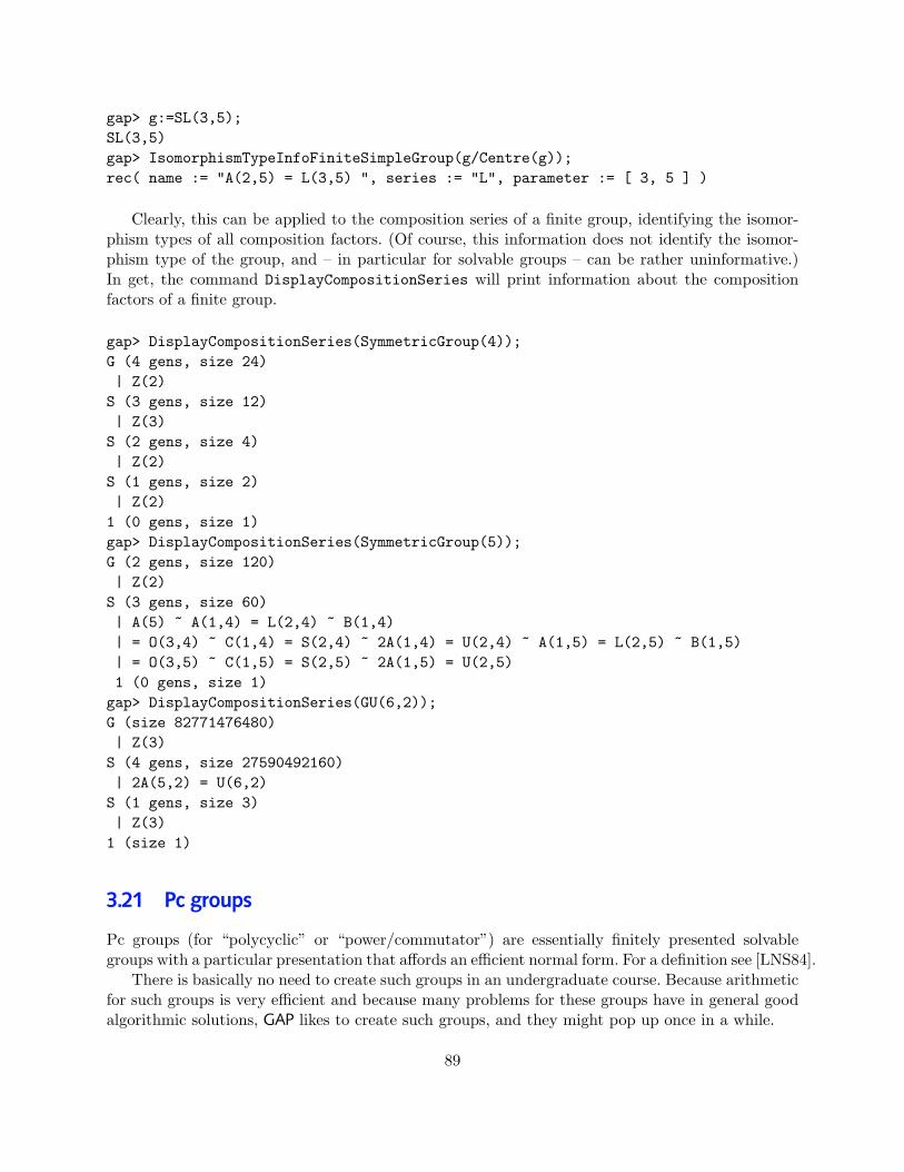
gap> g:=SL(3,5);SL(3,5)gap> IsomorphismTypeInfoFiniteSimpleGroup(g/Centre(g));rec( name := "A(2,5) = L(3,5) ", series := "L", parameter := [ 3, 5 ] )
Clearly, this can be applied to the composition series of a finite group, identifying the isomor-phism types of all composition factors. (Of course, this information does not identify the isomor-phism type of the group, and – in particular for solvable groups – can be rather uninformative.)In get, the command DisplayCompositionSeries will print information about the compositionfactors of a finite group.
gap> DisplayCompositionSeries(SymmetricGroup(4));G (4 gens, size 24)| Z(2)S (3 gens, size 12)| Z(3)S (2 gens, size 4)| Z(2)S (1 gens, size 2)| Z(2)1 (0 gens, size 1)gap> DisplayCompositionSeries(SymmetricGroup(5));G (2 gens, size 120)| Z(2)S (3 gens, size 60)| A(5) ~ A(1,4) = L(2,4) ~ B(1,4)| = O(3,4) ~ C(1,4) = S(2,4) ~ 2A(1,4) = U(2,4) ~ A(1,5) = L(2,5) ~ B(1,5)| = O(3,5) ~ C(1,5) = S(2,5) ~ 2A(1,5) = U(2,5)1 (0 gens, size 1)gap> DisplayCompositionSeries(GU(6,2));G (size 82771476480)| Z(3)S (4 gens, size 27590492160)| 2A(5,2) = U(6,2)S (1 gens, size 3)| Z(3)1 (size 1)
3.21 Pc groups
Pc groups (for “polycyclic” or “power/commutator”) are essentially finitely presented solvablegroups with a particular presentation that affords an efficient normal form. For a definition see [LNS84].
There is basically no need to create such groups in an undergraduate course. Because arithmeticfor such groups is very efficient and because many problems for these groups have in general goodalgorithmic solutions, GAP likes to create such groups, and they might pop up once in a while.
89
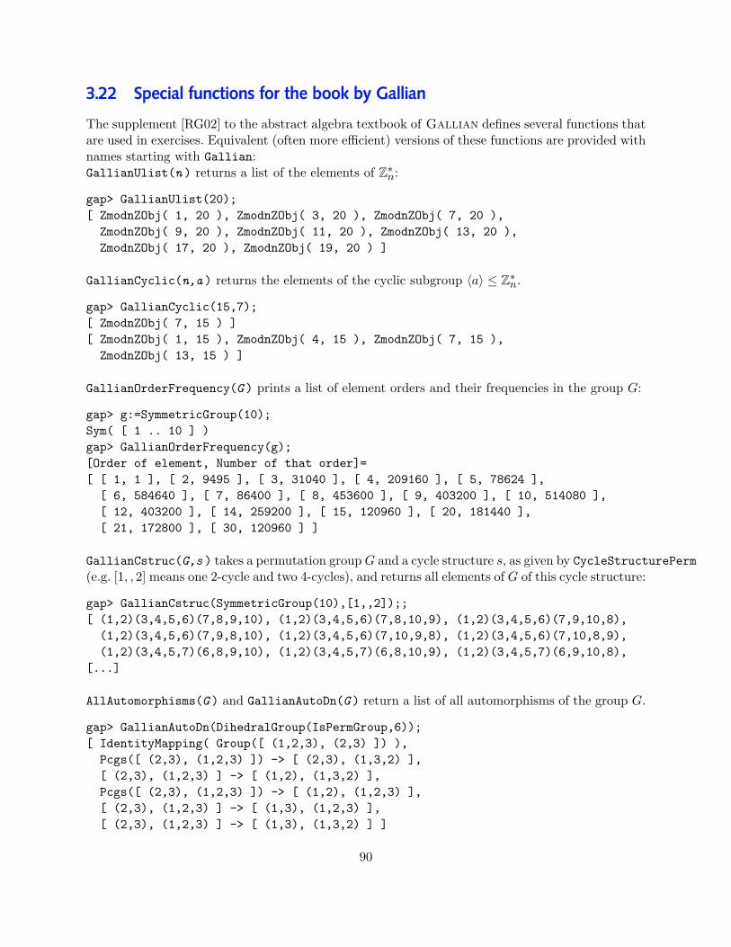
3.22 Special functions for the book by Gallian
The supplement [RG02] to the abstract algebra textbook of Gallian defines several functions thatare used in exercises. Equivalent (often more efficient) versions of these functions are provided withnames starting with Gallian:GallianUlist(n ) returns a list of the elements of Z∗n:
gap> GallianUlist(20);[ ZmodnZObj( 1, 20 ), ZmodnZObj( 3, 20 ), ZmodnZObj( 7, 20 ),ZmodnZObj( 9, 20 ), ZmodnZObj( 11, 20 ), ZmodnZObj( 13, 20 ),ZmodnZObj( 17, 20 ), ZmodnZObj( 19, 20 ) ]
GallianCyclic(n,a ) returns the elements of the cyclic subgroup 〈a〉 ≤ Z∗n.
gap> GallianCyclic(15,7);[ ZmodnZObj( 7, 15 ) ][ ZmodnZObj( 1, 15 ), ZmodnZObj( 4, 15 ), ZmodnZObj( 7, 15 ),ZmodnZObj( 13, 15 ) ]
GallianOrderFrequency(G ) prints a list of element orders and their frequencies in the group G:
gap> g:=SymmetricGroup(10);Sym( [ 1 .. 10 ] )gap> GallianOrderFrequency(g);[Order of element, Number of that order]=[ [ 1, 1 ], [ 2, 9495 ], [ 3, 31040 ], [ 4, 209160 ], [ 5, 78624 ],[ 6, 584640 ], [ 7, 86400 ], [ 8, 453600 ], [ 9, 403200 ], [ 10, 514080 ],[ 12, 403200 ], [ 14, 259200 ], [ 15, 120960 ], [ 20, 181440 ],[ 21, 172800 ], [ 30, 120960 ] ]
GallianCstruc(G,s ) takes a permutation groupG and a cycle structure s, as given by CycleStructurePerm(e.g. [1, , 2] means one 2-cycle and two 4-cycles), and returns all elements of G of this cycle structure:
gap> GallianCstruc(SymmetricGroup(10),[1,,2]);;[ (1,2)(3,4,5,6)(7,8,9,10), (1,2)(3,4,5,6)(7,8,10,9), (1,2)(3,4,5,6)(7,9,10,8),(1,2)(3,4,5,6)(7,9,8,10), (1,2)(3,4,5,6)(7,10,9,8), (1,2)(3,4,5,6)(7,10,8,9),(1,2)(3,4,5,7)(6,8,9,10), (1,2)(3,4,5,7)(6,8,10,9), (1,2)(3,4,5,7)(6,9,10,8),
[...]
AllAutomorphisms(G ) and GallianAutoDn(G ) return a list of all automorphisms of the group G.
gap> GallianAutoDn(DihedralGroup(IsPermGroup,6));[ IdentityMapping( Group([ (1,2,3), (2,3) ]) ),Pcgs([ (2,3), (1,2,3) ]) -> [ (2,3), (1,3,2) ],[ (2,3), (1,2,3) ] -> [ (1,2), (1,3,2) ],Pcgs([ (2,3), (1,2,3) ]) -> [ (1,2), (1,2,3) ],[ (2,3), (1,2,3) ] -> [ (1,3), (1,2,3) ],[ (2,3), (1,2,3) ] -> [ (1,3), (1,3,2) ] ]
90
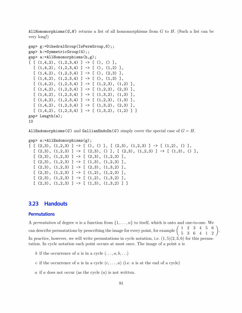
AllHomomorphisms(G,H ) returns a list of all homomorphisms from G to H. (Such a list can bevery long!)
gap> g:=DihedralGroup(IsPermGroup,6);;gap> h:=SymmetricGroup(4);;gap> a:=AllHomomorphisms(h,g);[ [ (1,4,2), (1,2,3,4) ] -> [ (), () ],[ (1,4,2), (1,2,3,4) ] -> [ (), (1,2) ],[ (1,4,2), (1,2,3,4) ] -> [ (), (2,3) ],[ (1,4,2), (1,2,3,4) ] -> [ (), (1,3) ],[ (1,4,2), (1,2,3,4) ] -> [ (1,2,3), (1,2) ],[ (1,4,2), (1,2,3,4) ] -> [ (1,2,3), (2,3) ],[ (1,4,2), (1,2,3,4) ] -> [ (1,3,2), (1,3) ],[ (1,4,2), (1,2,3,4) ] -> [ (1,2,3), (1,3) ],[ (1,4,2), (1,2,3,4) ] -> [ (1,3,2), (2,3) ],[ (1,4,2), (1,2,3,4) ] -> [ (1,3,2), (1,2) ] ]
gap> Length(a);10
AllEndomorphisms(G ) and GallianEndoDn(G ) simply cover the special case of G = H.
gap> a:=AllEndomorphisms(g);[ [ (2,3), (1,2,3) ] -> [ (), () ], [ (2,3), (1,2,3) ] -> [ (1,2), () ],[ (2,3), (1,2,3) ] -> [ (2,3), () ], [ (2,3), (1,2,3) ] -> [ (1,3), () ],[ (2,3), (1,2,3) ] -> [ (2,3), (1,2,3) ],[ (2,3), (1,2,3) ] -> [ (1,3), (1,2,3) ],[ (2,3), (1,2,3) ] -> [ (2,3), (1,3,2) ],[ (2,3), (1,2,3) ] -> [ (1,2), (1,2,3) ],[ (2,3), (1,2,3) ] -> [ (1,2), (1,3,2) ],[ (2,3), (1,2,3) ] -> [ (1,3), (1,3,2) ] ]
3.23 Handouts
Permutations
A permutation of degree n is a function from 1, . . . , n to itself, which is onto and one-to-one. We
can describe permutations by prescribing the image for every point, for example(
1 2 3 4 5 65 3 6 4 1 2
).
In practice, however, we will write permutations in cycle notation, i.e. (1, 5)(2, 3, 6) for this permu-tation. In cycle notation each point occurs at most once. The image of a point a is
b if the occurrence of a is in a cycle (. . . , a, b, . . .)
c if the occurrence of a is in a cycle (c, . . . , a) (i.e. a is at the end of a cycle)
a if a does not occur (as the cycle (a) is not written.
91

To write a permutation p =(
1 2 . . . np1 p2 . . . pn
)(i.e. p maps i to pi) in cycle form use the following
procedure:While there are points not processed
Let a be a point that is not processed.Write (aLet i := pa (i.e. the image of a under p).While i 6= a
Write , iLet i = pi
end whileWrite ).If the cycle just completed has length 1, delete it.
end whileFor example, for the permutation given above, we start by picking a = 1 and obtain i = p1 = 5.
We write (1,, As 1 6= 5 we continue as (1, 5 and get i = p5 = 1. This closes the cycle and we havewritten (1, 5). Next we pick a = 2, writing (1, 5)(2. Then i = p2 = 3 and we write (1, 5)(2, 3. Nexti = p3 = 6 and write (1, 5)(2, 3, 6. As i = p6 = 2 we close the cycle to (1, 5)(2, 3, 6). Finally we picka = 4. As i = p4 = 4 the cycle gets closed immediately: (1, 5)(2, 3, 6)(4) and – having length one –deleted, giving the result (1, 5)(2, 3, 6).
It is common to pick a always as small as possible, resulting in cycles starting with their smallestelements each, though it is possible to write cycles differently, e.g. (1, 5)(2, 3, 6) = (5, 1)(3, 6, 2).
Important Observation: different cycles of a permutation never share points!
Arithmetic in cycle notation As the image of a point under a permutation is its successorin the cycle, the image under the inverse is the predecessor. We can thus invert a permutation bysimply reverting all of its cycles (possibly rotating each cycle afterwards to move the smallest pointfirst): (1, 5)(2, 3, 6)−1 = (5, 1)(6, 3, 2) = (1, 5)(2, 6, 3), (1, 2, 3, 4, 5)−1 = (5, 4, 3, 2, 1) = (1, 5, 4, 3, 2).
To multiply permutations, trace through the images of points, and build a new permutationfrom the images, as when translating into cycle structure. For example, suppose we want to multiply(1, 5)(2, 3, 6) · (1, 6, 4)(3, 5). The image of 1 is 5 under the first, and the image of 5 is 3 under thesecond permutation. Tus the result will start (1, 3 . . .. 3 maps to 6 and 6 to 4, thus (1, 3, 4 . . .. 4 isfixed first and then maps to 1. So the first cycle of the result is (1, 3, 4). We pick a next point 2. 2is mapped to 3 and 3 to 5, so we have (1, 3, 4)(2, 5 . . .. 5 is mapped to 1 and 1 to 6 and (as thereare no points left) we are done: (1, 5)(2, 3, 6) · (1, 6, 4)(3, 5) = (1, 3, 4)(2, 5, 6).
Permutations in GAP In GAP we can write permutations in cycle form and multiply (or invertthem). The multiplication order is the same as used in class (again, remember that the book usesa reversed order):
gap> (1,2,3)*(2,3);(1,3)gap> (2,3)*(1,2,3);(1,2)gap> a:=(1,2,3,4)(6,5,7);(1,2,3,4)(5,7,6)
92

gap> a^2;(1,3)(2,4)(5,6,7)gap> a^-1;(1,4,3,2)(5,6,7)gap> b:=(1,3,5,7)(2,6,8);(1,3,5,7)(2,6,8)gap> a*b;(1,6,7,8,2,5)(3,4)gap> a*b*a^-1;(1,7,8)(2,6,5,4)
Groups generated by elements
We have seen so far two ways of specifying subgroups: By listing explicitly all elements, or byspecifying a defining property of the elements. In some cases neither variant is satisfactory tospecify certain subgroups, and it is preferrable to specify a subgroup by generating elements.
Definition: Let G be a group and a1, a2, . . . , an ∈ G. The set
〈a1, a2, . . . , an〉 =
bε11 · b
ε22 · · · · · b
εkk | k ∈ N0 = 0, 1, 2, 3, , . . ., bi ∈ a1, . . . , an, εi ∈ 1,−1
(with the convention that for k = 0 the product over the empty list is e) is called the subgroup ofG generated by a1, . . . , an.
Note: If G is finite, we can – similarly to the subgroup test – forget about inverses in the expo-nents.
Example: Let G = S4 and a1 = (1, 2)(3, 4), a2 = (1, 4)(2, 3). Then
〈a1, a2〉 = (), a1, a2, a1 · a1 = (), a1 · a2 = (1, 3)(2, 4), a2 · a−11 = (1, 3)(2, 4), a1 · a2 · a1 = a2, . . .
(Careful: In this particular case a1 · a2 = a2 · a1, though S4 is not abelian.) We find that regardlesshow long we form products, we never get elements other than (), a1, a2, a1 · a2. Similarly, it is nothard to see that S4 = 〈(1, 2), (1, 2, 3, 4)〉
Note: If you had already linear algebra you know this idea of “generation” in the form of spanningsets and bases. While the concept for groups is very similar, it is not possible to translate theconcept of “dimension”: Different (even “independent”) generating sets for a subgroup in generalwill contain a different number of generators.
We now want to show that 〈a1, a2, . . . , an〉 is always a subgroup:
Theorem: Let G be a group and a1, a2, . . . , an ∈ G. Then H := 〈a1, a2, . . . , an〉 ≤ G.Proof: For k = 0 we get the identity, thus e ∈ H and thus H 6= ∅. Now use the criterion forsubgroups:
93

Let x, y ∈ H. Then (by the definition of H) there exist k, l ∈ N0 and elements bi, cj ∈ a1, . . . , an,εi, δj ∈ ±1 such that:
x = bε11 · bε22 · · · · · b
εkk , y = cδ11 · c
δ22 · · · · · c
δll .
Note that y−1 = c−δll · c−δl−1
l−1 · · · · · c−δ11 . Thus
x · y−1 = bε11 · bε22 · · · · · b
εkk · c
−δll · c−δl−1
l−1 · · · · · c−δ11 ,
which has the form of an element of H. Thus H is a subgroup.
Note: If S ≤ G is a subgroup with a1, . . . , an ∈ S, then certainly all those products must beelements of S (as S is closed under multiplication). Thus 〈a1, a2, . . . , an〉 is the smallest subgroupof G containing all the elements a1, a2, . . . , an.
Special Case: A special case is that of only one generator, i.e. of cyclic subgroups. Then we havein the definition that 〈a〉 = bε11 ·b
ε22 · · · · ·b
εkk with bi ∈ a. We can now use the rules for exponents
and write everything as a single power of a. Thus we get:
〈a〉 = ax | x ∈ Z = a0, a1, a−1, a2, a−2, a3, a−3, . . .
is the set of all powers of a which agrees with the definition from the book.
How to calculate elements In some circumstances, it can be desirable to obtain an elementlist from generators. Since the operation in a group is associative, we have that
bε11 · bε22 · · · · · b
εkk = (bε11 · b
ε22 · · · · · b
εk−1
k−1 ) · bεkk .
We can therefore obtain the elements by the following process in an recursive way:
Starting with the identity, multiply all elements “so far” with all generators (and theirinverses) until nothing new is obtained.
The following description of the algorithm is more formal:
1. Write down a “start” mark.
2. Write down the identity e (all products of length 0).
3. Mark the (current) end of the list with an “end” mark. Let x run through all elements in this listbetween the “start” and “end” mark.
4. Let y run through all the generators a1, · · · an.
5. Form the products x · y and x · y−1. If the result is not yet in the list, add it at the end.
6. If you have run through all x, y, and you find that you added new elements to the end of the list (afterthe “end” mark), make the “end” mark the “start” mark and go back to step 3.
7. Otherwise you have found all elements in the group.
If the group is finite at some point longer products must give the same result as shorter products (whichhave been computed before), thus the process will terminate.
94

Example: Let G = U(48) = 1, 5, 7, 11, 13, 17, 19, 23, 25, 29, 31, 35, 37, 41, 43, 47 and a1 = 5,a2 = 11. We calculate that a−1
1 = 29, a−12 = 35.
We start by writing down the identity (S and E are start and end mark respectively):
S, 1, E
Now we form the products of all written down elements with a1, a2, a−11 and a−1
2 :
1 · 5 = 5, 1 · 11 = 11, 1 · 29 = 29, 1 · 35 = 35,
So our list now is 1, S, 5, 11, 29, 35, E. Again (back to step 3) we run through all elements writtendown so far, and form products:
5 · 5 = 25, 5 · 11 = 7, 5 · 29 = 1, 5 · 35 = 31, 11 · 5 = 7, 11 · 11 = 25, 11 · 29 = 31, 11 · 35 = 1,29 · 5 = 1, 29 · 11 = 31, 29 · 29 = 25, 29 · 35 = 7, 35 · 5 = 31, 35 · 11 = 1, 35 · 29 = 7, 35 · 35 = 25
The underlined entries are not new and thus did not get added again. Our new list therefore is1, 5, 11, 29, 35, S, 25, 7, 31, E. Again we form products:
25 · 5 = 29, 25 · 11 = 35, 25 · 29 = 5, 25 · 35 = 11, 7 · 5 = 35, 7 · 11 = 29, 7 · 29 = 11, 7 · 35 = 5,31 · 5 = 11, 31 · 11 = 5, 31 · 29 = 35, 31 · 35 = 29
Now no new elements were found. Thus we got all elements of the subgroup, and we have 〈5, 11〉 =1, 5, 7, 11, 25, 29, 31, 35. (The ordering of elements now is unimportant, as we list the subgroup asa set.)
Expression as words If we are giving a group by generators this means that each of its elementscan be written – not necessarily uniquely – as a product of generators (and inverses). The processof enumerating all elements in fact gives such an expression. For example we trace back that31 = 5 · 11−1.
For larger groups this of course can become very tedious, but it is a method that can easily beperformed on a computer.
Example: (GAP calculation) Consider the permutation group generated by (1, 2, 3, 4, 5) and(1, 2)(3, 4):
gap> a1:=(1,2,3,4,5);(1,2,3,4,5)gap> a2:=(1,2)(3,4);(1,2)(3,4)gap> G:=Group(a1,a2);Group([ (1,2,3,4,5), (1,2)(3,4) ])gap> Elements(G);[ (), (3,4,5), (3,5,4), (2,3)(4,5), (2,3,4), (2,3,5), (2,4,3), (2,4,5),
95

(2,4)(3,5), (2,5,3), (2,5,4), (2,5)(3,4), (1,2)(4,5), (1,2)(3,4),(1,2)(3,5), (1,2,3), (1,2,3,4,5), (1,2,3,5,4), (1,2,4,5,3), (1,2,4),(1,2,4,3,5), (1,2,5,4,3), (1,2,5), (1,2,5,3,4), (1,3,2), (1,3,4,5,2),(1,3,5,4,2), (1,3)(4,5), (1,3,4), (1,3,5), (1,3)(2,4), (1,3,2,4,5),(1,3,5,2,4), (1,3)(2,5), (1,3,2,5,4), (1,3,4,2,5), (1,4,5,3,2), (1,4,2),(1,4,3,5,2), (1,4,3), (1,4,5), (1,4)(3,5), (1,4,5,2,3), (1,4)(2,3),(1,4,2,3,5), (1,4,2,5,3), (1,4,3,2,5), (1,4)(2,5), (1,5,4,3,2), (1,5,2),(1,5,3,4,2), (1,5,3), (1,5,4), (1,5)(3,4), (1,5,4,2,3), (1,5)(2,3),(1,5,2,3,4), (1,5,2,4,3), (1,5,3,2,4), (1,5)(2,4) ]
gap> Length(Elements(G));60gap> Order(G);60
If we wanted to express an element of the group as a word in the generators, we could use thecommand Factorization. (This command in fact internally enumerates all elements and storesword expressions for each. the word returned therefore is as short as possible. The functionalityhowever is limited by the available memory – if we cannot store all group elements it will fail.)
For example for the same group as before we express a (random) element and check that theresult is the same:
gap> Factorization(G,(1,5)(3,4));x1^-2*x2*x1^2gap> a1^-2*a2*a1^2;(1,5)(3,4)
Application: Sort the sequence E,D,B,C,A by performing only swaps of adjacent elements:Considering the positions, we want to perform the permutation (1, 5)(2, 4, 3). The swaps of adjacentelements are the permutations a1 = (1, 2), a2 = (2, 3), a3 = (3, 4), a4 = (4, 5). Using GAP, wecalculate:
gap> a1:=(1,2);(1,2)gap> a2:=(2,3);(2,3)gap> a3:=(3,4);(3,4)gap> a4:=(4,5);(4,5)gap> G:=Group(a1,a2,a3,a4);Group([ (1,2), (2,3), (3,4), (4,5) ])gap> Factorization(G,(1,5)(2,4,3));x1*x2*x1*x3*x2*x4*x3*x2*x1
This means swap positions (in this order) 1/2, 2/3, 1/2, 3/4, 2/3, 4/5, 3/4, 2/3. 1/2 and you getthe right arrangement (try it out!)
96

Puzzles Many puzzles can be described in this way: Each state of the puzzle corresponds to apermutation, the task of solving the puzzle then corresponds to expressing the permutation as aproduct of generators. Example 7 on p.107 in the book is an example of this.
The 2 × 2 × 2 Rubik’s Cube in GAP As an example of a more involved puzzle consider the2× 2× 2 Rubik’s cube. We label the facelets of the cube in the following way:
21
43
109
1211
2221
2423
65
87
1413
1615
1817
2019
top
left right back
bottom
front
We now assume that we will fix the bottom right corner (i.e. the corner labelled with 16/19/24) inspace – this is to make up for rotations of the whole cube in space. We therefore need to consideronly three rotations, front, top and left. The coresponding permutations are (for clockwise rotationwhen looking at the face):
gap> top:=(1,2,4,3)(5,17,13,9)(6,18,14,10);;gap> left:=(1,9,21,20)(5,6,8,7)(3,11,23,18);;gap> front:=(3,13,22,8)(4,15,21,6)(9,10,12,11);;gap> cube:=Group(top,left,front);Group([(1,2,4,3)(5,17,13,9)(6,18,14,10),(1,9,21,20)(3,11,23,18)(5,6,8,7),(3,13,22,8)(4,15,21,6)(9,10,12,11) ])
gap> Order(cube);3674160
By defining a suitable mapping first (for the time being consider this command as a black box) wecan choose nicer names – T, L and F – for the generators:
gap> map:=EpimorphismFromFreeGroup(cube:names:=["T","L","F"]);[ T, L, F ] -> [ (1,2,4,3)(5,17,13,9)(6,18,14,10),(1,9,21,20)(3,11,23,18)(5,6,8,7), (3,13,22,8)(4,15,21,6)(9,10,12,11) ]
We now can use the command Factorization to express permutations in the group as word ingenerators. The reverse sequence of the inverse operations therefore will turn the cube back to itsoriginal shape. For example, suppose the cube has been mixed up in the following way:
97

621
2013
2310
1814
52
2412
48
1722
97
161
113
1519
This corresponds to the permutation
gap> move:=(1,15,20,4,6,2,21)(3,17,8,5,22,7,13)(9,14,11,18,12,23,10)
(1 has gone in the position where 15 was, 2 has gone in the position of 21, and so on.) We expressthis permutation as word in the generators:
gap> Factorization(cube,move);T*F*L*T*F*T
We can thus bring the cube back to its original position by turning each counterclockwise top,front,top,left,front,top.
Larger puzzles If we want to do something similar for larger puzzles, for example the 3× 3× 3cube, the algorithm used by Factorization runs out of memory. Instead we would need to use adifferent algorithm, which can be selected by using the map we used for defining the name. Thealgorithm used then does not guarantee any longer a shortest word, in our example:
gap> PreImagesRepresentative(map,move);T*L^-2*T^-1*L*T*L^-2*T^-2*F*T*F^-1*L^-1*F*T^-1*F^-1*L*T*L*T^-2*F*T*F^-1*T*F*T^-1*F^-2*L^-1*F^2*L
(Note that the code uses some randomization, your mileage may vary.)
Solving Rubik’s Cube by hand
In this note, we want to determine a strategy for solving the2× 2× 2 Rubik’s cube by hand. (Again, similar approacheswork for other puzzles, this one is just small enough to befeasible in class.)Remember that we label the faces of the cube as shown andfix the piece (16/19/24) in space. The group of symmetriesthen is
G = 〈 top = (1, 2, 4, 3)(5, 17, 13, 9)(6, 18, 14, 10),left = (1, 9, 21, 20)(5, 6, 8, 7)(3, 11, 23, 18),front = (3, 13, 22, 8)(4, 15, 21, 6)(9, 10, 12, 11) 〉
21
43
109
1211
2221
2423
65
87
1413
1615
1817
2019
top
left right back
bottom
front
98

The basic idea now is to place pieces in the right position (e.g. in “layers” of the cube), andthen continue with movements that leave these correctly placed pieces unmoved. Moving the firstpieces is usually easy; the hard work is to find suitable elements in the stabilizer or the positionsfilled so far.
We will choose the positions to be filled in a way that guarantees that many of the originalgenerators fix the chosen points. This will automatically make for some stabilizer generators beingrepresented by short words. Concretely, we will fill the positions starting in the order (23,22,21)and then work on the top layer.
We start by computing the orbit of 23. This is done in a similar way as we would enumerate allgroup elements: We calculate the image of all points processed so far under all generators, until nonew images arise. We also keep track of group elements which map 23 to the possible images.
It is possible to do these slightly tedious calculations with GAP. The following set of commands willcalculate the orbit and keep track of words that yield the same image. (We work with words, as they areeasier to read than images.)
map:=EpimorphismFromFreeGroup(cube:names:=["T","L","F"]);gens:=GeneratorsOfGroup(cube);letters:=GeneratorsOfGroup(Source(map)); # corresponding lettersorb:=[23]; # the orbit being builtwords:=[One(letters[1])]; # words that produce the right imagesfor x in orb dofor i in [1..Length(gens)] doimg:=x^gens[i];if not img in orb thenAdd(orb,img);p:=Position(orb,x);Add(words,words[p]*letters[i]);
fi;od;
od;
As a result we get the following orbit and representatives:
Orbit 23 18 14 3 10 1 11 13 6 12 2Rep e L LT L2 LT 2 L2T L3 L2F LT 3 LT 2F L2T 2
Orbit 9 22 8 4 5 21 7 15 17 20Rep L2TL L2F 2 LT 3L LT 3F L2TLT L2TL2 LT 3L2 LT 3F 2 L2TLT 2 L2TL3
The crucial idea for stabilizer elements (apart from the obvious ones, such as top rotation here)now is the following: Suppose that the image of an orbit element x under a generator g gives an oldorbit element y. Then Repx · g ·Rep−1
y moves the starting element (here 23) to itself and thereforelies in the stabilizer. (One can show2, that all of these elements generate the stabilizer.)
In our example, we find that 23T = 23, so e · T · e−1 = T must lie in the stabilizer. Similarly11F = 9, so L3 · F · (L2TL) lies in the stabilizer, and so on.
2This is called Schreier’s lemma, see for example Holt: Handbook of Computational Group Theory
99

By computing group orders we find that we just need a few elements for generation, namely
C1 := StabG(23) =⟨T, F, L−1TL
⟩(It is worth noticing that the construction process tends to produce elements of the form ABA−1.If you consult any printed solution strategy, this kind of shape indeed abounds.) As far as solvingthe cube is concerned, it is very easy to get a few initial positions right. Therefore we don’t aim fora systematic strategy yet, but keep the stabilizer generators for the next level.
The next position we work with is 22, similarly as above (again, there is a nontrivial calculationinvolved in showing that these three elements suffice, if one takes just a few random elements thereis no a-priori guarantee that they would do) we get
C2 := StabG(22, 23) =⟨T, L−1TL, FTF−1
⟩Next (this is completing the bottom layer), we stabilize 21. This is wherethe stabilizer becomes interesting, as far as continuing to solve the puzzleis concerned. A repeated application gets
C3 := StabG(21, 22, 23) =⟨T, LT−1L−1T−1F−1LF
⟩The second generator here is chosen amongst many other possibilitiesas being of shortest possible length. Its action on the cube is the per-mutation (1, 17, 5, 14, 18, 2)(4, 10, 13), i.e. two pieces are swapped (andturned) and one piece is turned. If we only consider the positions (butnot rotations) of the top four pieces, it is not hard to see (homework)that together with the top rotation this will let us place every piecein its right position up to rotation. (This means, we are stabilizing thesets 1, 5, 18, 2, 14, 17, 3, 6, 9 and 4, 10, 13 — formally we areconsidering a different group action here, namely one on the cubies.)What is left now is to orient the top 4 pieces suitably. By looking throughstabilizer generators we find the element L−1FL−1FT−1L−1T 2F 2LTwith the permutation (3, 6, 9)(4, 13, 10). It rotates the top two front cu-bies in opposite directions. Clearly similar movements are possible tothe top cubies on the other sides, by rotating the whole cube in space.By applying these moves for front, left and back, we can determine theplacement of three of the top cubies arbitrarily.
(1,17,5,14,18,2)(4,10,13)
(3,6,9)(4,13,10)
We now claim that this will actually solve the cube completely. We know that [G : C1] =|orbG(23)| = 24−3 = 21 (on the whole cube, the piece in position 23 can be moved in all positions,short of the three fixed ones). Similarly, when stabilizing position 23, we can (this can be easilychecked by trying out the moves permitted in C1) move the piece in position 22 to all places, butthe 3 fixed ones (16/19/24) and the three that share a cubie with 23 (7/20/23), so [C1 : C2] = 18.By a similar argument [C2 : C3] = 15.
Under the stabilizer C3 we have seen that we can correctly place the four cubies in all possiblepermutations, thus the group stabilizing the cubie positions has index 24 in C3. Using that |G| =
100
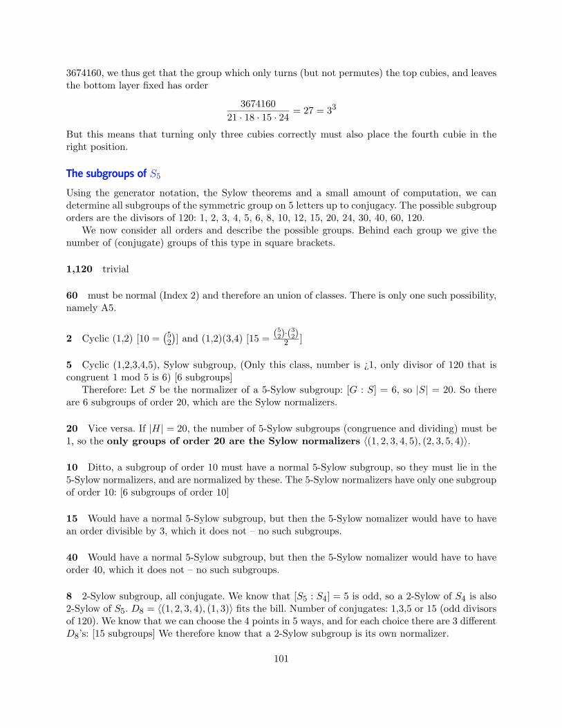
3674160, we thus get that the group which only turns (but not permutes) the top cubies, and leavesthe bottom layer fixed has order
367416021 · 18 · 15 · 24
= 27 = 33
But this means that turning only three cubies correctly must also place the fourth cubie in theright position.
The subgroups of S5
Using the generator notation, the Sylow theorems and a small amount of computation, we candetermine all subgroups of the symmetric group on 5 letters up to conjugacy. The possible subgrouporders are the divisors of 120: 1, 2, 3, 4, 5, 6, 8, 10, 12, 15, 20, 24, 30, 40, 60, 120.
We now consider all orders and describe the possible groups. Behind each group we give thenumber of (conjugate) groups of this type in square brackets.
1,120 trivial
60 must be normal (Index 2) and therefore an union of classes. There is only one such possibility,namely A5.
2 Cyclic (1,2) [10 =(52
)] and (1,2)(3,4) [15 = (5
2)·(32)
2 ]
5 Cyclic (1,2,3,4,5), Sylow subgroup, (Only this class, number is ¿1, only divisor of 120 that iscongruent 1 mod 5 is 6) [6 subgroups]
Therefore: Let S be the normalizer of a 5-Sylow subgroup: [G : S] = 6, so |S| = 20. So thereare 6 subgroups of order 20, which are the Sylow normalizers.
20 Vice versa. If |H| = 20, the number of 5-Sylow subgroups (congruence and dividing) must be1, so the only groups of order 20 are the Sylow normalizers 〈(1, 2, 3, 4, 5), (2, 3, 5, 4)〉.
10 Ditto, a subgroup of order 10 must have a normal 5-Sylow subgroup, so they must lie in the5-Sylow normalizers, and are normalized by these. The 5-Sylow normalizers have only one subgroupof order 10: [6 subgroups of order 10]
15 Would have a normal 5-Sylow subgroup, but then the 5-Sylow nomalizer would have to havean order divisible by 3, which it does not – no such subgroups.
40 Would have a normal 5-Sylow subgroup, but then the 5-Sylow nomalizer would have to haveorder 40, which it does not – no such subgroups.
8 2-Sylow subgroup, all conjugate. We know that [S5 : S4] = 5 is odd, so a 2-Sylow of S4 is also2-Sylow of S5. D8 = 〈(1, 2, 3, 4), (1, 3)〉 fits the bill. Number of conjugates: 1,3,5 or 15 (odd divisorsof 120). We know that we can choose the 4 points in 5 ways, and for each choice there are 3 differentD8’s: [15 subgroups] We therefore know that a 2-Sylow subgroup is its own normalizer.
101

4 Must be conjugate to a subgroups of the 2-Sylow subgroup. Therefore the following three areall possibilities:
Cyclic 〈(1, 2, 3, 4)〉 [15 = 5 · 3: choose the point off, then there are 3 subgroups each]
not cyclic 〈(1, 2), (3, 4)〉 [15, ditto ]
not cyclic 〈(1, 2)(3, 4), (1, 3)(2, 4)〉 [5 copies: choose the point off]
3 Cyclic 〈(1, 2, 3)〉 [(53
)= 10 subgroups as (1,2,3) and (1,3,2) lie in the same group] Also Sylow,
thus the 3-Sylow normalizer must have index 10, order 12.
6 A group of order 6 must have a normal 3-Sylow subgroup, and therefore lie in a 3-Sylownormalizer, which is (conjugate to) 〈(1, 2, 3), (1, 2), (4, 5)〉. We can find 3×2 = 〈(1, 2, 3)(4, 5)〉 (cyclic)[(53
)= 10 groups], S3 = 〈(1, 2, 3), (1, 2)〉 [
(53
)= 10 copies]) and 〈(1, 2, 3), (1, 2)(4, 5)〉 (isomorphic
S3) [(53
)= 10 copies].
30 Can have 1 or 10 3-Sylow subgroups. If 1, it would be in the Sylow normalizer, contradic-tion as before. If it is 10, it contains all 3-Sylow subgroups, but 〈(1, 2, 3), (3, 4, 5)〉 has order 60,Contradiction.
12 If it has a normal 3-Sylow subgroup, it must be amongst the 3-Sylow normalizers 〈(1, 2, 3), (1, 2), (4, 5)〉[We know already there are 10 such groups].
If not, it contains 4 3-Sylow subgroups, i.e. 8 elements of order 3. Thart leaves space only for 3elements of order 2, the 2-Sylow subgroup (or order 4) therefore must be normal, and its normalizerhas index at most 10, i.e. it has at most 10 conjugates. This leaves 〈(1, 2)(3, 4), (1, 3)(2, 4)〉, whosenormalizer is S4. (its normal in S4, and S4 has the right order). Inspecting S4, we find it has onlyone subgroup of order 12, namely A4 = 〈(1, 2, 3), (2, 3, 4)〉 with [5, same as the number of S4’s]conjugates.
24 We know there are [5] copies of S4, namely the point stabilizers. We now want to show that isall: (There are 15 groups of order 24, so we can’t that easily determine the structure alone from theorder.) Its 2-Sylow subgroup must be a 2-Sylow of S5, so WLOG its 2-Sylow is D8. Now considerthe orbit of 1 under this subgroup. It must have length at least 4 (that’s under D8), but the orbitlength must divide 24. So it cannot be 5. But that means that the subgroup fixes one point andthus is S4.
3.24 Problems
Exercise 22. Determine the elements and the multiplication table (sometimes called Cayley table)for the group of symmetries of an equilateral triangle.
Exercise 23. Let G = 〈(1, 2, 3, 8)(4, 5, 6, 7), (1, 7, 3, 5)(2, 6, 8, 4)〉 be a permutation group generatedby two permutations.Determine the elements of G and their orders. What is |G|?
102

Exercise 24.
Consider a puzzle, as depicted on the side, whichconsists of two overlapping rings filled with balls.By moving the balls along either ring one can mixthe balls and then try to restore the original situa-tion.In this problem we will consider a simplified ver-sion, that consists only of 8 balls, arranged as givenin the second picture on the right.We will describe this state by a scheme of the form:
1 32
4 57
6 8
a) Write permutations for the rotation % around theleft circle and the rotation σ around the right circle.
Image: Egner,Puschel: Proc ISSAC 1998
51 2 3
76 84
b) Using the Factorization command (see below), give sequences of operations that will returnthe following states back to the original:
4 51
2 86
3 7
,
2 13
4 57
6 8
(Check that the results you got actually work!)
Exercise 25. a) Show that one can calculate ab mod n by 2 log2(b) multiplications of numbers mod-ulo n. (Hint: Consider b in binary form and calculate a2 mod n, a4 mod n,. . . . The GAP commandPowerMod(a,b,n) implements this.)b) Show that n := 2307 − 1 is not prime, by finding a number a such that an mod n 6= a.
Exercise 26. The German “Enigma” encryption machine, used in the second world war, produced(by a set of moving rotors) in each step a permutation σ ∈ S26 (Interpreting the numbers 1-26 asletters in the alphabet.)
103

a) Show that it is not always possible to use the samesetting (i.e. the same permutation σ) to encrypt anddecrypt. (This causes problems for dumb operators –they would need to change settings between encryptionor decryption.)b) To ease handling for the operators (who understoodlittle math), the German military had the “clever”idea to add a “plug-board” (on the picture in frontof the machine) that swapped pairs of letters (thiscreates a permutation π that has a cycle type as(1, 2)(3, 4)(5, 6) · · · (25, 26)) and to feed the encryptionthrough the old mechanism (σ), then through the plug-board, and in reverse back through the mechanism.So the encryption performed now was of the formµ = σ−1πσ.Show that this encryption is self-reverting, i.e. thatµ2 = 1. (Thus the same setting could be used for en-cryption and decryption.)c) Show that µ must be the product of thirteen 2-cycles.d) How many possibile σ exist. How many possible µexists? Explain, based on this count, why consequen-tially the “clever” idea was really stupid (and indeedwas one of the reasons the code could be broken).
Source:http:// www. math. miami. edu/ ~ harald/ enigma/
enigma. html
Exercise 27. Let G = 〈(1, 2, 3), (2, 3, 4)〉. The following GAP command determines all subgroupsof G:
s:=Union(List(ConjugacyClassesSubgroups(G),Elements));
Draw a subgroup lattice (as done in the lecture for the symmetries of a square). Which of thesubgroups are cyclic? Which ones are normal? Does G have a subgroup of order k for every kdividing |G|?(Useful GAP commands: IsSubset(S,T), IsCyclic(S), IsNormal(G,S).)
104

Exercise 28. Let G ≤ Sn be a permutation group and Ω = a, b | 1 ≤ a 6= b,≤ n the class ofall 2-element subsets of numbers in 1, . . . , n (i.e. the set a, b is considered the same as b, a).We know that |Ω| =
(n2
). We define an action α of G on Ω by acting on the entries:
α (a, b, g) := g(a), g(b)
a) Show that this defines a group action.b) For G = D8 = 〈(1, 2, 3, 4), (1, 3)〉, determine the orbits of G on Ω.
Exercise 29.
A dodecahedron has 60 symmetries, namely
1 identityA 6 · 4 = 24 rotations through face centers,B 2 · 10 = 20 rotations around corners,C 15 rotations around edge centers.
a) For elements of type A,B and C, determine the orbits (of the cyclicsubgroup generated by this element) on the faces.b) Determine how many different ways (up to symmetry) exist, to colorthe faces of the dodecahedron in green and gold.
AB
B
C
Exercise 30. The following six pictures depict all faces of a mixed-up 2× 2× 2 Rubik’s cube (withthe same face labelling as the example in class):
105

a) Suppose you unfold the cube to a cross-shaped diagram (as on the handout in class), give thecorrect labeling of the faces.b)Write down a permutation that describes the mixup of this cube from its original position.c) Using GAP, determine a sequence of moves to bring the cube back to its original position.
Exercise 31. Prove or disprove:a) U(20) and U(24) are isomorphic.b) U(20) and D4 are isomorphic.c) U(20) and U(15) are isomorphic.
106

4
-
Linear Algebra
Linear Algebra is the basis for most concrete calculations. GAP accordingly has a strong supportof linear algebra functions. These functions exisst on two levels – a lower level of matrices and rowvectors, as well as a hiogher level of abstract vector spaces and bases (which perform all work viacoefficient vectors and the lower level functions).
The linear algebra functions work for any arbitrary field available in GAP, however no “numer-ical” or approximate algorithms are available.
4.1 Operations for matrices
Vectors (typically considered as row vectors) in GAP are simply lists of their entries and matricesare lists of their rows as vectors – see section 1.3.
Matrices can be added, multiplied and (if invertible) inverted using the standard arithmetic +,* and ^-1 (respectively Inverse) operations.
Matrices returned by arithmetic operations (as well as by many functions) are immutable (i.e.cannot be modified). To obtain a modifyable copy of such a matrix M , one can use the commandMutableCopyMat(M ).
For a matrix M , TransposedMat(M ) returns the transpose and Display(M ) pretty-prints thematrix. Print(LaTeX(M )) prints LaTeX commands for typesetting the matrix (this is a conveniencefeature when using GAP to set up matrices for typesetting, e.g. in a homework or exam).
gap> M:=[[1,2,3],[4,5,6],[7,8,9]];[ [ 1, 2, 3 ], [ 4, 5, 6 ], [ 7, 8, 9 ] ]gap> TransposedMat(M);[ [ 1, 4, 7 ], [ 2, 5, 8 ], [ 3, 6, 9 ] ]gap> Display(last);[ [ 1, 4, 7 ],[ 2, 5, 8 ],[ 3, 6, 9 ] ]
gap> Print(LaTeX(M));\left(\beginarrayrrr%1&2&3\\%4&5&6\\%
107

7&8&9\\%\endarray\right)%
Rank(M ) determines the rank of a matrix and NullspaceMat(M ) a list of basis vectors of therow nullspace (i.e. those vectors x such that x · M = 0). For a vector y in the row space of M ,SolutionMat(M ,y ) returns one vector x such that x · M = y (and fail if no solution exists).
TriangulizedMat(M ) (synonym RREF) returns the reduced row echelon form of M . (The activeversion TriangulizeMat(M ) will change M to this form.)
gap> Rank(M);2gap> NullspaceMat(M);[ [ 1, -2, 1 ] ]gap> SolutionMat(M,[1,1,1]);[ -1/3, 1/3, 0 ]gap> TriangulizedMat(M);[ [ 1, 0, -1 ], [ 0, 1, 2 ], [ 0, 0, 0 ] ]
There are no separate operations for column nullspace or column solutions, to obtain these oneneeds to work with the transposed matrix.
Creating particular Matrices
NullMat(a ,b ,x ) creates an a × b matrix whose entries are 0 · x (this allows the creation of nullmatrices over different fields. IdentityMat(a ,x ) does the same for the a -dimensional identitymatrix.
For a list L , DiagonalMat(L ) creates a square diagonal matrix with the specified diagonalentries.
gap> NullMat(5,3,1);[ [ 0, 0, 0 ], [ 0, 0, 0 ], [ 0, 0, 0 ], [ 0, 0, 0 ], [ 0, 0, 0 ] ]gap> NullMat(5,3,Z(2));<a 5x3 matrix over GF2>gap> IdentityMat(4,9);[ [ 1, 0, 0, 0 ], [ 0, 1, 0, 0 ], [ 0, 0, 1, 0 ], [ 0, 0, 0, 1 ] ]gap> IdentityMat(4,Z(3));[ [ Z(3)^0, 0*Z(3), 0*Z(3), 0*Z(3) ], [ 0*Z(3), Z(3)^0, 0*Z(3), 0*Z(3) ],
[ 0*Z(3), 0*Z(3), Z(3)^0, 0*Z(3) ], [ 0*Z(3), 0*Z(3), 0*Z(3), Z(3)^0 ] ]gap> DiagonalMat([1,2,3]);[ [ 1, 0, 0 ], [ 0, 2, 0 ], [ 0, 0, 3 ] ]gap> DiagonalMat([Z(5),Z(5^2)]);[ [ Z(5), 0*Z(5) ], [ 0*Z(5), Z(5^2) ] ]
RandomMat(a ,b ,ring ) creates a random a × b matrix with entries in ring . If ring is anintegral domain, RandomInvertibleMat(a ,ring ) creates a random matrix over ring whose de-terminant is nonzero (but not necessarily a unit in ring ).
RandomUnimodularMat(n ) creates an n × n matrix with integer entries whose determinant is±1.
108
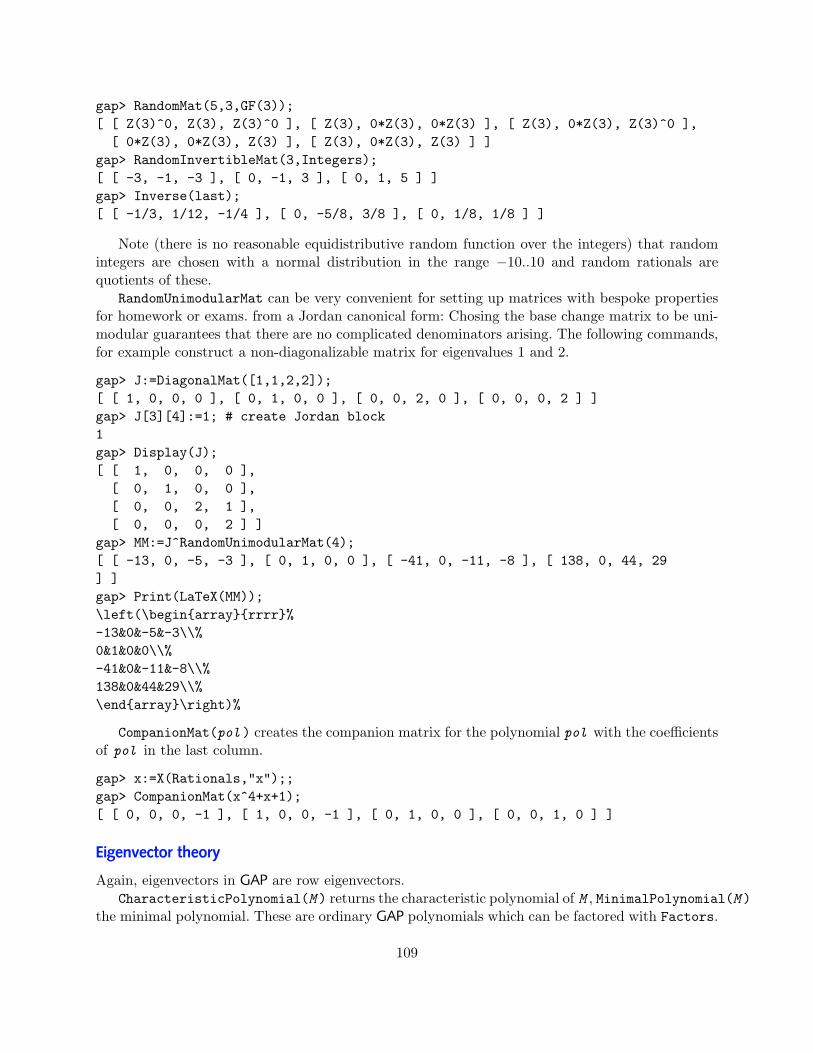
gap> RandomMat(5,3,GF(3));[ [ Z(3)^0, Z(3), Z(3)^0 ], [ Z(3), 0*Z(3), 0*Z(3) ], [ Z(3), 0*Z(3), Z(3)^0 ],[ 0*Z(3), 0*Z(3), Z(3) ], [ Z(3), 0*Z(3), Z(3) ] ]
gap> RandomInvertibleMat(3,Integers);[ [ -3, -1, -3 ], [ 0, -1, 3 ], [ 0, 1, 5 ] ]gap> Inverse(last);[ [ -1/3, 1/12, -1/4 ], [ 0, -5/8, 3/8 ], [ 0, 1/8, 1/8 ] ]
Note (there is no reasonable equidistributive random function over the integers) that randomintegers are chosen with a normal distribution in the range −10..10 and random rationals arequotients of these.
RandomUnimodularMat can be very convenient for setting up matrices with bespoke propertiesfor homework or exams. from a Jordan canonical form: Chosing the base change matrix to be uni-modular guarantees that there are no complicated denominators arising. The following commands,for example construct a non-diagonalizable matrix for eigenvalues 1 and 2.
gap> J:=DiagonalMat([1,1,2,2]);[ [ 1, 0, 0, 0 ], [ 0, 1, 0, 0 ], [ 0, 0, 2, 0 ], [ 0, 0, 0, 2 ] ]gap> J[3][4]:=1; # create Jordan block1gap> Display(J);[ [ 1, 0, 0, 0 ],[ 0, 1, 0, 0 ],[ 0, 0, 2, 1 ],[ 0, 0, 0, 2 ] ]
gap> MM:=J^RandomUnimodularMat(4);[ [ -13, 0, -5, -3 ], [ 0, 1, 0, 0 ], [ -41, 0, -11, -8 ], [ 138, 0, 44, 29] ]gap> Print(LaTeX(MM));\left(\beginarrayrrrr%-13&0&-5&-3\\%0&1&0&0\\%-41&0&-11&-8\\%138&0&44&29\\%\endarray\right)%
CompanionMat(pol ) creates the companion matrix for the polynomial pol with the coefficientsof pol in the last column.
gap> x:=X(Rationals,"x");;gap> CompanionMat(x^4+x+1);[ [ 0, 0, 0, -1 ], [ 1, 0, 0, -1 ], [ 0, 1, 0, 0 ], [ 0, 0, 1, 0 ] ]
Eigenvector theory
Again, eigenvectors in GAP are row eigenvectors.CharacteristicPolynomial(M ) returns the characteristic polynomial of M , MinimalPolynomial(M )
the minimal polynomial. These are ordinary GAP polynomials which can be factored with Factors.
109

Eigenvalues(field M ) returns the eigenvalues of M over field . Eigenvectors(field M ) re-turns a list of a maximal linear independent set of eigenvectors.
gap> CharacteristicPolynomial(MM);x^4-6*x^3+13*x^2-12*x+4gap> Factors(last);[ x-2, x-2, x-1, x-1 ]gap> MinimalPolynomial(MM);x^3-5*x^2+8*x-4gap> Eigenvalues(Rationals,MM);[ 2, 1 ]gap> Eigenvectors(Rationals,MM);[ [ 1, 0, 3, 1 ], [ 1, 0, 1/2, 1/4 ], [ 0, 1, 0, 0 ] ]gap> Eigenvalues(Rationals,M);[ 0 ]# to get all eigenvalues we will need the root of 33gap> Collected(Factors(Discriminant(CharacteristicPolynomial(M))));[ [ 2, 2 ], [ 3, 7 ], [ 11, 1 ] ]gap> Eigenvalues(CF(33),M);[ 0, (15+3*Sqrt(33))/2, (15-3*Sqrt(33))/2 ]gap> Eigenvectors(CF(33),M);[ [ 1, -2, 1 ], [ 1, (9+Sqrt(33))/12, (3+Sqrt(33))/6 ],[ 1, (9-Sqrt(33))/12, (3-Sqrt(33))/6 ] ]
Normal Forms
Amongst the normal forms of matrices that are typically considered in an abstract algebra course,the Smith Normal Form, or Elementary Divisors Normal Form form is probably the most funda-mental. By using only ring operations, it transforms a matrix into diagonal form with subsequentdiagonal entries dividing each other. It can be used to solve linear systems over the integers, deter-mine the structure of an abelian group, and is the key to most other normal forms of matrices.
While this normal form is defined for any PID, the lack of a general GCD algorithm restrictsthis in practice to euclidean rings.
For an matrix M , defined over an Euclidean ring R , ElementaryDivisorsMat(R ,M ) determinesthe diagonal entries of the Smith Normal Form of M . ElementaryDivisorsMat(M ) tries to choosea suitable ring, depending on the entries of M .
In many concrete applications it is necessary to also obtaind transforming matrices. This isdone by ElementaryDivisorsTransformationsMat(R ,M ). It returns a record with components.rowtrans and .coltrans that give the matrices that will transform M to the normal form. (Therecord may – as in the example – contain further components.)
gap> ElementaryDivisorsMat(M);[ 1, 3, 0 ]gap> r:=ElementaryDivisorsTransformationsMat(M);rec( rowtrans := [ [ 1, 0, 0 ], [ 4, -1, 0 ], [ 1, -2, 1 ] ],coltrans := [ [ 1, -2, 1 ], [ 0, 1, -2 ], [ 0, 0, 1 ] ],
110

normal := [ [ 1, 0, 0 ], [ 0, 3, 0 ], [ 0, 0, 0 ] ], rank := 2, signdet :=0,rowC := [ [ 1, 0, 0 ], [ 0, 1, 0 ], [ 0, 0, 1 ] ],rowQ := [ [ 1, 0, 0 ], [ 4, -1, 0 ], [ 1, -2, 1 ] ],colC := [ [ 1, 0, 0 ], [ 0, 1, 0 ], [ 0, 0, 1 ] ],colQ := [ [ 1, -2, 1 ], [ 0, 1, -2 ], [ 0, 0, 1 ] ] )
gap> r.rowtrans*M*r.coltrans=r.normal;true
While these functions work for arbitrary euclidean rings (for example also for matrices withpolynomial entries), the implementation for the special case of the integers is far mor sophisticated,while the general case only implements a basic version.
gap> charmat:=x^0*MM-MM^0*x;[ [ -x-13, 0, -5, -3 ], [ 0, -x+1, 0, 0 ], [ -41, 0, -x-11, -8 ],[ 138, 0, 44, -x+29 ] ]
gap> r:=ElementaryDivisorsTransformationsMat(charmat);rec(coltrans := [ [ 0, -5/37, 20/9, 5*x-13 ], [ 0, -1/37*x-25/37, 4/9*x-11/9,
x^2-4*x+4 ], [ -1/5, 1/37*x+13/37, -4/9*x+59/9, -x^2+16*x-37 ],[ 0, 0, -185/9, -44*x+118 ] ],
normal := [ [ 1, 0, 0, 0 ], [ 0, 1, 0, 0 ], [ 0, 0, x-1, 0 ],[ 0, 0, 0, x^3-5*x^2+8*x-4 ] ],
rowtrans := [ [ 1, 0, 0, 0 ], [ -1/5*x-11/5, 1, 1, 0 ],[ 44/185*x^2+366/185*x+66/37, -44/37*x+118/37, -44/37*x+118/37, 1 ],[ -1/9*x^3-7/9*x^2+1/3*x+11/3, 5/9*x^2-20/9*x+20/9,
5/9*x^2-20/9*x+29/9, -4/9*x+11/9 ] ] )gap> DiagonalOfMat(r.normal);[ 1, 1, x-1, x^3-5*x^2+8*x-4 ]gap> r.rowtrans*charmat*r.coltrans;[ [ 1, 0, 0, 0 ], [ 0, 1, 0, 0 ], [ 0, 0, x-1, 0 ],[ 0, 0, 0, x^3-5*x^2+8*x-4 ] ]
gap> Inverse(r.rowtrans);[ [ 1, 0, 0, 0 ], [ 0, 1/37*x^2+24/37*x-25/37, -4/9*x+11/9, -1 ],[ 1/5*x+11/5, -1/37*x^2-24/37*x+62/37, 4/9*x-11/9, 1 ],[ -44/5, 44/37*x-118/37, 1, 0 ] ]
As they typically require the ability to take square roots (and for complete factorization of theminimal polynomial), GAP does not provide a QR decomposition or Singular Values.
4.2 Problems
Exercise 32. a) Let
A :=
60 −60 48 −232−9 9 −6 36−21 21 −18 80
111

Determine the Smith Normal Form of A as well as transforming matrices P and Q.b) Let b := (−76, 15, 23)T . Determine all integer solutions to the system Ax = b.
112

5
-
Fields and Galois Theory
Rationals, Cyclotomic fields and finite fields already have been described in previous sections. Thischapter is about Field extensions and particular functions for Galois theory over the rationals.
5.1 Field Extensions
For a field F and an irreducible polynomial f with coefficients in F , the command AlgebraicExtension(F ,f )(short: AlgebraicExtension(f ) if the field is unambiguous), constructs F [x]/(f ) as a field exten-sion of F . if the field is unambiguous), constructs K = F [x]/(f ) as a field extension of F . WhieleGAP tries to embed F into K for purposes of mixed arithmetic, elements of K differ from elementsof F and will for example be printed differently (and will not compare as equal to elements of F ):Elements of K that are in the natural image of F are printed by the representative in F , precededby an exclamation mark. Other elements are printed as a polynomial in a, where a represents aroot of f . This root can be obtained from K as RootOfDefiningPolynomial(K).
gap> e:=AlgebraicExtension(Rationals,pol);<algebraic extension over the Rationals of degree 5>gap> a:=RootOfDefiningPolynomial(e);agap> a^5;!7gap> (3*a+4)^3;27*a^3+108*a^2+144*a+64gap> (3*a+4)^17;242646788160000*a^4+345206482560000*a^3+478557123373125*a^2+706130877097500*a+1109261977360000
To create polynomials over these extensions, it is necessary to create a new indeterminate. UsingValue with the new indeterminate is the easiest way to embed polynomials over the extension.Polynomial factorization over the extensions is possible, but can quickly get expensive if the degreegets higher.
gap> y:=X(e,"y");y
113

gap> epol:=Value(pol,y); # embedy^5+(!-7)gap> Factors(epol);[ y+(-a), y^4+a*y^3+a^2*y^2+a^3*y+a^4 ]
If the polynomial defines a normal extension, it will split into linear factors and the Galois groupconsists simply of those maps that map the primitive root a to any of the other roots.
gap> pol:=x^8+3*x^4+1;x^8+3*x^4+1gap> e:=AlgebraicExtension(Rationals,pol);<algebraic extension over the Rationals of degree 8>gap> y:=X(e,"y");ygap> epol:=Value(pol,y); # embedy^8+!3*y^4+!1gap> RootsOfUPol(e,epol);[ -a^7-2*a^3, -a^7-3*a^3, -a, -a^5-2*a, a^7+2*a^3, a^7+3*a^3, a, a^5+2*a ]
Polynomials for iterated extensions
At the moment it is not possible to form iterated algebraic extensions. the following process howevercan be used to construct polynomials for larger extensions. (The theory behind this is explainedin [WR76].) Some description of this process is given in exercise 36.
Suppose that f is an irreducible polynomial over F and E = F (a) the extension of F obtained byadjoining one root a of f . Let g ∈ E[y] be an irreducible polynomial. We now consider g ∈ F [x, y] byreplacing all occurrences of a in g by x. Then the resultant r := resx(f(x), (g(x, y)) is a polynomialover F that has a root of g as root. If r is squarefree, it will define a larger extension. If notsquarefreeness can be acchieved, by replacing g with a new polynomial h such that h(y) = g(y+b·a)for a suitable integer b.
gap> pol:=x^5-7;;e:=AlgebraicExtension(Rationals,pol);;y:=X(e,"y");;<algebraic extension over the Rationals of degree 5>gap> a:=RootOfDefiningPolynomial(e);;epol:=Value(pol,y);; # embedgap> g:=epol/(y-a);y^4+a*y^3+a^2*y^2+a^3*y+a^4gap> Factors(g);[ y^4+a*y^3+a^2*y^2+a^3*y+a^4 ]gap> z:=X(Rationals,"z"); # since ‘y’ is already usedzgap> gpol:=z^4+x*z^3+x^2*z^2+x^3*z+x^4;x^4+x^3*z+x^2*z^2+x*z^3+z^4gap> r:=Resultant(pol,gpol,x);z^20-28*z^15+294*z^10-1372*z^5+2401gap> Gcd(r,Derivative(r));z^15-21*z^10+147*z^5-343
114

So the resultant was not squarefree. We replace y by y − 2a and try again
gap> h:=Value(g,y-2*a);y^4+(-7*a)*y^3+19*a^2*y^2+(-23*a^3)*y+11*a^4gap> hpol:=z^4+(-7*x)*z^3+(19*x^2)*z^2+(-23*x^3)*z+11*x^4;11*x^4-23*x^3*z+19*x^2*z^2-7*x*z^3+z^4gap> r:=Resultant(pol,hpol,x);z^20+546*z^15+482356*z^10+18083646*z^5+386683451gap> Gcd(r,Derivative(r));1
Thus r now is a polynomial which defines an extension in which x5 − 7 has (at least) two roots –in fact it is the splitting field. Alas typically such calculations will end up very quickly with messycoefficients.
gap> e:=AlgebraicExtension(Rationals,r);<algebraic extension over the Rationals of degree 20>gap> a:=RootOfDefiningPolynomial(e);agap> y:=X(e,"y");ygap> epol:=Value(pol,y); # embedy^5+(!-7)gap> Factors(epol);[ y+(9/116963000*a^16+97/2387000*a^11+85483/2387000*a^6+271197/341000*a),y+(-1/18865000*a^16-81/2695000*a^11-9987/385000*a^6-56283/55000*a),y+(1/29240750*a^16+36/2088625*a^11+4768/298375*a^6-31433/85250*a),y+(3/292407500*a^16+139/20886250*a^11+36451/5967500*a^6+183141/213125*a),y+(-1/14620375*a^16-72/2088625*a^11-9536/298375*a^6-11192/42625*a) ]
We can now factor r to obtain from its roots the images of a under the elements of the Galoisgroup. (In this particular example, working by hand and with 5
√7 and ζ7 would be easier, the merit
of this approach is that it works in general.)
gap> roots:=RootsOfUPol(e,epol);gap> rootpols:= # express as polynomials in x[ -9/116963000*x^16-97/2387000*x^11-85483/2387000*x^6-271197/341000*x,1/18865000*x^16+81/2695000*x^11+9987/385000*x^6+56283/55000*x,-1/29240750*x^16-36/2088625*x^11-4768/298375*x^6+31433/85250*x,-3/292407500*x^16-139/20886250*x^11-36451/5967500*x^6-183141/213125*x,1/14620375*x^16+72/2088625*x^11+9536/298375*x^6+11192/42625*x ];
gap> List(rootpols,z->Value(z,a))=roots; # just checktruegap> aimgs:=RootsOfUPol(e,Value(r,y)); # this takes very long[ -23/292407500*a^16-859/20886250*a^11-32453/852500*a^6-25976/213125*a,-1/5316500*a^16-823/8354500*a^11-1901/21700*a^6-208331/170500*a, a,111/584815000*a^16+8271/83545000*a^11+153211/1705000*a^6+2640133/1705000*a,-1/11696300*a^16-391/8354500*a^11-47339/1193500*a^6-226429/170500*a,
115

-57/584815000*a^16-4507/83545000*a^11-573219/11935000*a^6-4286241/1705000*a,-59/584815000*a^16-389/7595000*a^11-545233/11935000*a^6-87927/155000*a,3/41772500*a^16+1791/41772500*a^11+214237/5967500*a^6+2059103/852500*a,19/584815000*a^16+1399/83545000*a^11+23399/1705000*a^6-1185483/1705000*a,37/292407500*a^16+1301/20886250*a^11+344989/5967500*a^6-71221/213125*a,-4/73101875*a^16-29/949375*a^11-84131/2983750*a^6-52309/38750*a,-17/116963000*a^16-251/3341800*a^11-161771/2387000*a^6-19733/341000*a,3/29240750*a^16+108/2088625*a^11+14304/298375*a^6+76201/85250*a,51/292407500*a^16+3951/41772500*a^11+500317/5967500*a^6+1968613/852500*a,1/16709000*a^16+43/1519000*a^11+67093/2387000*a^6-67/248*a,-12/73101875*a^16-3673/41772500*a^11-231933/2983750*a^6-2088549/852500*a,17/584815000*a^16+1627/83545000*a^11+27397/1705000*a^6+2133561/1705000*a,-9/584815000*a^16-369/83545000*a^11-71843/11935000*a^6+3002093/1705000*a,1/10443125*a^16+29/542500*a^11+136573/2983750*a^6+92019/77500*a,1/20886250*a^16+221/10443125*a^11+58909/2983750*a^6-310322/213125*a ]
Lets pick, for example the 7th root image and see what the corresponding automorphism doesto the roots of the original polynomial pol :
gap> img:=aimgs[7];-59/584815000*a^16-389/7595000*a^11-545233/11935000*a^6-87927/155000*agap> Value(r,img); # indeed a root of the polynomial defining the field!0gap> List(rootpols,z->Position(roots,Value(z,img)));[ 4, 3, 1, 5, 2 ]
So the automorphism of e , defined by mapping a to img will permute the roots of pol as indicated.We can can to the same for all possible images and thus represent the Galois group by permutationsand use this to establish its structure as the Frobenius group of order 20.
gap> perms:=List(aimgs,> im->PermList(List(rootpols,z->Position(roots,Value(z,im)))));[ (1,2)(4,5), (1,2,5,3), (), (1,3,5,2), (1,3)(2,4), (1,3,4,5), (1,4,5,2,3),(2,4,5,3), (2,5)(3,4), (2,3,5,4), (1,5,3,4,2), (1,4,2,5), (1,4)(3,5),(1,4,3,2), (1,2,4,3,5), (1,5,4,3), (1,5)(2,3), (1,5,2,4), (1,3,2,5,4),(1,2,3,4) ]
gap> Length(perms);20gap> Size(Group(perms));20gap> TransitiveIdentification(Group(perms));3gap> TransitiveGroup(5,3);F(5) = 5:4
116

5.2 Galois groups over the rationals
If f ∈ Q[x] is an irreducible polynomial, we can consider the splitting field K of f as a Galoiosextension over Q. A typical problem in Galois theory is to determine the Galois group G of suchan extension, however the difficulty of hand arithmetic, and in particular of representing automor-phisms, makes it hard to consider extensions that are not cyclotomic or with a dihedral Galoisgroup. One fundamental issue is already that to represent automorphisms of an extension, it isnecessary to represent the extension K/Q. If [K : Q] is several hundered (something which is easilyacchieved already for degree 8), this becomes infeasible.
A way around this problem is to consider the Galois group more abstractly: Every Galoisautomorphism will permute the roots of f . If f is of degree n, this yields a homomorphism ϕ : G→Sn. The kernel of ϕ is trivial (automorphisms that fix all roots, fix all of K) and the image Gϕ is atransitive group of degree n (if G acted intransitively on the roots, the roots in one orbit would yielda factor of f). In other words, as long as we do not aim to apply the homomorphism (the methodsbelow will identify Gϕ without constructing ϕ), we can consider G as a transitive subgroup of Sn.
The first approach uses a theorem of Dedekind and Frobenius (a nice proof, completely suitablefor an advance undergraduate course, can be found in van der Waerden’s book [vdW71]), thatstates that – for a prime p not dividing any denominators and such that f mod p is squarefree – theGalois group H of f mod p over Fp can be considered as a subgroup of Gϕ. However H is cyclic andits cycle shape (as a permutation in Sn) is given simply by the degrees of the irreducible factors off mod p.
The theorem of Chebotarev [SL96] (whose proof is far beyond any undergraduate course)strengthens this to the result that in the limit over all primes, every element of G arises in subgroupsH with the same frequency.
By factororing f modulo a set of primes, one thus can get some idea of the structure of G. Inparticular, we can identify the case that Gϕ = Sn since this is implied by the existence of certaincycle shapes (See [DSar]). Handout 5.3 gives some examples of such a process.)
An automated implementation of this process (for values of n ≤ 30) is implemented by thefunction ProbabilityShapes(f ). It returns a list of index numbers (as transitive groups of theappropriate degree) of the most likely candidates for the Galois group of the splitting field of f .In the following example, the splitting field has (most likely) degree 8 (i.e. the group acts regularlyon the roots) and Galois group isomorphic to the dihedral group of order 8.
gap> pol:=x^8+3*x^4+1;x^8+3*x^4+1gap> Factors(pol);[ x^8+3*x^4+1 ]gap> ProbabilityShapes(pol);[ 4 ]gap> TransitiveGroup(8,4);D_8(8)=[4]2
A perfect (nonprobabilistic) identification – albeit at potentially very long runtime in largerexamples – is accheived by GaloisType(f ) which returns not a list but just the number of theactual Galois group type.
117

gap> GaloisType(pol);4
In either case what is identified is the Sn-class of the image Gϕ, no identification of the rootstakes place.
5.3 Handouts
Identification of a Galois group by Cycle Shapes
We create a polynomial and find that it is squarefee modulo all primes > 7.
gap> x:=X(Rationals,"x");;f:=x^8-16*x^4-98;;gap> Set(Factors(Discriminant(f)));[ -2, 2, 3, 7 ]gap> l:=Filtered([8..1000],IsPrimeInt);;Length(l);164
Lets consider the first such prime, 11. We reduce f modulo 11 and find that it is the product oftwo factors of degree 4.
gap> p:=l[1];11gap> UnivariatePolynomial(GF(p),CoefficientsOfUnivariatePolynomial(f)> *One(GF(p)),1);x_1^8+Z(11)^9*x_1^4+Z(11)^0gap> fmod:=UnivariatePolynomial(GF(p),CoefficientsOfUnivariatePolynomial(f)> *One(GF(p)),1);x_1^8+Z(11)^9*x_1^4+Z(11)^0gap> List(Factors(fmod),Degree);[ 4, 4 ]
The ‘Collected’ command transforms such a list into a nicer form: 2 factors of degree 4. We start alist in which we collect this information and do the same calculation in a loop over all other primes.
gap> shape:=Collected(List(Factors(fmod),Degree));[ [ 4, 2 ] ]gap> a:=[];;gap> Add(a,shape);
gap> for i in [2..Length(l)] do> p:=l[i];> fmod:=UnivariatePolynomial(GF(p),CoefficientsOfUnivariatePolynomial(f)> *One(GF(p)),1);> shape:=Collected(List(Factors(fmod),Degree)); Add(a,shape);> od;
118
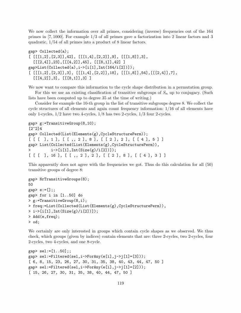
We now collect the information over all primes, considering (inverse) frequencies out of the 164primes in [7, 1000]. For example 1/3 of all primes gave a factorization into 2 linear factors and 3quadratic, 1/54 of all primes into a product of 8 linear factors.
gap> Collected(a);[ [[[1,2],[2,3]],42], [[[1,4],[2,2]],9], [[[1,8]],3],[[[2,4]],23],[[[4,2]],45], [[[8,1]],42] ]
gap>List(Collected(a),i->[i[1],Int(164/i[2])]);[ [[[1,2],[2,3]],3], [[[1,4],[2,2]],18], [[[1,8]],54],[[[2,4]],7],[[[4,2]],3], [[[8,1]],3] ]
We now want to compare this information to the cycle shape distribution in a permutation group.For this we use an existing classification of transitive subgroups of Sn up to conjugacy. (Such
lists have been computed up to degree 35 at the time of writing.)Consider for example the 10-th group in the list of transitive subgroups degree 8. We collect the
cycle structures of all elements and again count frequency information: 1/16 of all elements haveonly 1-cycles, 1/2 have two 4-cycles, 1/8 has two 2-cycles, 1/3 four 2-cycles.
gap> g:=TransitiveGroup(8,10);[2^2]4gap> Collected(List(Elements(g),CycleStructurePerm));[ [ [ ], 1 ], [ [ ,, 2 ], 8 ], [ [ 2 ], 2 ], [ [ 4 ], 5 ] ]gap> List(Collected(List(Elements(g),CycleStructurePerm)),> i->[i[1],Int(Size(g)/i[2])]);[ [ [ ], 16 ], [ [ ,, 2 ], 2 ], [ [ 2 ], 8 ], [ [ 4 ], 3 ] ]
This apparently does not agree with the frequencies we got. Thus do this calculation for all (50)transitive groups of degree 8:
gap> NrTransitiveGroups(8);50gap> e:=[];;gap> for i in [1..50] do> g:=TransitiveGroup(8,i);> freq:=List(Collected(List(Elements(g),CycleStructurePerm)),> i->[i[1],Int(Size(g)/i[2])]);> Add(e,freq);> od;
We certainly are only interested in groups which contain cycle shapes as we observed. We thuscheck, which groups (given by indices) contain elements that are: three 2-cycles, two 2-cycles, four2-cycles, two 4-cycles, and one 8-cycle.
gap> sel:=[1..50];;gap> sel:=Filtered(sel,i->ForAny(e[i],j->j[1]=[3]));[ 6, 8, 15, 23, 26, 27, 30, 31, 35, 38, 40, 43, 44, 47, 50 ]gap> sel:=Filtered(sel,i->ForAny(e[i],j->j[1]=[2]));[ 15, 26, 27, 30, 31, 35, 38, 40, 44, 47, 50 ]
119

gap> sel:=Filtered(sel,i->ForAny(e[i],j->j[1]=[4]));[ 15, 26, 27, 30, 31, 35, 38, 40, 44, 47, 50 ]gap> sel:=Filtered(sel,i->ForAny(e[i],j->j[1]=[,,2]));[ 15, 26, 27, 30, 31, 35, 38, 40, 44, 47, 50 ]gap> sel:=Filtered(sel,i->ForAny(e[i],j->j[1]=[,,,,,,1]));[ 15, 26, 27, 35, 40, 44, 47, 50 ]
8 Groups remain. All but the first contain elements of shapes we did not observe, but we can alsoconsider frequencies:
gap> esel;[ [[[],32],[[,,,,,,1],4],[[,,2],4],[[2],16],[[3],4],[[4],6]],[[[],64],[[,,,,,,1],4],[[,,1],16],[[,,2],5],[[2],10],[[2,,1],16],[[3],8],[[4],4]],
[[[],64],[[,,,,,,1],4],[[,,2],3],[[1],16],[[2],10],[[2,,1],8],[[3],16],[[4],12]],
[[[],128],[[,,,,,,1],8],[[,,1],32],[[,,2],4],[[1],32],[[1,,1],16],[[2],12],[[2,,1],4],[[3],10],[[4],7]],
[[[],192],[[,,,,,,1],4],[[,,1],16],[[,,2],16],[[,2],6],[[1,,,,1],6],[[2],32],[[2,,1],16],[[3],8],[[4],14]],
[[[],384],[[,,,,,,1],8],[[,,,,1],12],[[,,1],32],[[,,2],6],[[,2],12],[[1],96],[[1,,,,1],12],[[1,,1],16],[[1,2],12],[[2],21],[[2,,1],10],[[3],13],[[4],15]],
[[[],1152],[[,,,,,,1],8],[[,,1],96],[[,,2],10],[[,1],72],[[,1,1],12],[[,2],18],[[1],96], [[1,,,,1],6],[[1,,1],16],[[1,1],12],[[2],27 ],[[2,,1],6],[[2,1],24],[[3],32],[[4],34]],
[[[],40320],[[,,,,,,1],8],[[,,,,,1],7],[[,,,,1],12],[[,,,1],30],[[,,1],96],[[,,2],32],[[,1],360],[[,1,,1],15],[[,1,1],12],[[,2],36],[[1],1440],[[1,,,,1],12],[[1,,,1],10],[[1,,1],16],[[1,1],36],[[1,2],36],[[2],192],[[2,,1],32],[[2,1],24],[[3],96],[[4],384]]]
Comparing with the frequencies in the group again, we find that the first group (index 15) givesthe best correspondence overall.
gap> List(Collected(a),i->[i[1],Int(164/i[2])]);[ [[[1,2],[2,3]],3], [[[1,4],[2,2]],18], [[[1,8]],54],[[[2,4]],7],[[[4,2]],3], [[[8,1]],3] ]
(The group has order 32, it has a structure (C2 ×D8) o C2.)
5.4 Problems
Exercise 33. The GAP list Primes contains the 168 prime numbers < 1000. Determine the degreedistributions (and their frequencies) when factoring x4 + 4x3 + 6x2 + 4x− 4 modulo these primes.How frequently (roughly) does each degree distribution occur? (You might want to concentrate on thefrequency of primes for which the polynomial will split into linear factors.) Repeat the experimentfor x4 − 10x2 + 1 and x4 + 3x+ 1. What frequencies occur in these cases?
120

Exercise 34. There are 5 classes of transitive groups of degree 4: 1 : 〈(1, 2, 3, 4)〉 ∼= C4, 2 :〈(1, 2)(3, 4), (1, 3)(2, 4)〉 ∼= V4, 3 : 〈(1, 2, 3, 4), (1, 3)〉 ∼= D8, 4 : 〈(1, 2, 3), (2, 3, 4)〉 ∼= A4, and 5 :〈(1, 2, 3, 4), (1, 2)〉 ∼= S4. Using GAP, find polynomials of degree 4 that have each of these groups asGaloisType.
Exercise 35. Determine the irreducible polynomials of degree dividing 4 over F2 and show thattheir product is x16 − x.(Hint: You can verify the result in GAP:
x:=X(GF(2),"x");Factors(x^16-x);
Exercise 36. Let α be algebraic over F with minimal polynomial m(x) ∈ F [x] and F (α) ∼=F [x]/ 〈m(x)〉 the corresponding algebraic extension. Suppose that g(x) ∈ F (α)[x] and that β isa root of g(x). Consider h(x, y) ∈ F [x, y] such that g(x) = h(x, α) (i.e. we replace occurrences ofα in the coefficients of g by a new variable y). Then the resultant r(x) = resy (h(x, y),m(y)) is apolynomial that has β as root, i.e. r(β) = 0.(Note: r(x) is not necessarily irreducible, the minimal polynomial of β is an irreducible factor ofr.)
For example, suppose we want to construct a rational polynomial that has a root of x4 +5x+ 3√
2as a root. Set p(x) = x3 − 2 (minimal polynomial of 3
√2) and h(x, y) = x4 + 5x+ y.
gap> x:=X(Rationals,"x");;y:=X(Rationals,"y");;gap> p:=x^3-2;;gap> h:=x^4+5*x+y;;gap> r:=Resultant(h,Value(p,y),y); # The Value command takes p in y-x^12-15*x^9-75*x^6-125*x^3-2gap> Factors(r);[ -x^12-15*x^9-75*x^6-125*x^3-2 ]
We can use this method to construct iterative extensions, in particular splitting fields. We takean irreducible polynomial p and construct the field F (α), adjoining one root of α of p. Then wefactor p over F (α) and take an irreducible factor q(x). We replace x by x+ k · α for some integerk (this is needed to avoid just getting a power of p again, as all roots of q are also roots of p andthus have the same minimal polynomial. Typically k = 1 works. Proof for this later.) The resultantthen defines the field with two roots adjoined and so on.
For example, we can construct the splitting field of x3 − 2 over Q:
gap> p:=x^3-2;;gap> e:=AlgebraicExtension(Rationals,p);<algebraic extension over the Rationals of degree 3>gap> a:=PrimitiveElement(e); # a is alphaagap> pe:=Value(p,X(e)); # make it a polynomial over e.x_1^3+(!-2)gap> qs:=Factors(pe);q:=qs[2];;
121

[ x_1+(-a), x_1^2+a*x_1+a^2 ]gap> Value(q,X(e)+a); $ Note X(e) is the proper ‘‘x’’x_1^2+3*a*x_1+3*a^2gap> h:=x^2+3*y*x+3*y^2;x^2+3*x*y+3*y^2gap> r:=Resultant(h,Value(p,y),y);x^6+108gap> Factors(r); # As r is irreducible it now defines the double extension[ x^6+108 ]gap> e:=AlgebraicExtension(Rationals,r); # now verify that p splits<algebraic extension over the Rationals of degree 6>gap> Factors(Value(p,X(e)));[ x_1+(1/36*a^4-1/2*a), x_1+(1/36*a^4+1/2*a), x_1+(-1/18*a^4) ]
(If p would not split here we would take again one of the factors and repeat the process.) Note thatthe printed a now is a root of r, which is (from the way we modified q, replacing x by x+ 3
√2) the
difference of two roots of p, e.g. we can assume it it be γ := 3√
2(1− e2πi3 ). Indeed, we can calculate
γ6 = −108, thus it is a root of our r. Considering the irreducible factors of r calculated above,
we can also check (by tedious complex arithmetic) thatγ4
36− γ
2= − 3√
2,γ4
36+γ
2= − 3√
2e2πi3 , and
− 118γ4 = − 3
√2e
4πi3 , so these are indeed the factors.
If r defines the splitting field of p and we factor r over this field Q[x]/ 〈r〉 = Q(γ), we get roots(we’ll see later why r must split as well over this field). In the above example:
gap> s:=RootsOfUPol(Value(r,X(e)));[ -1/12*a^4-1/2*a, -a, 1/12*a^4-1/2*a, 1/12*a^4+1/2*a, a, -1/12*a^4+1/2*a ]
We thus know the possible automorphisms of Q(γ), for example γ 7→ −γ, or γ 7→ −γ4
12− γ
2.
We know (in this example) that Q(γ) = Q( 3√
2, ζ = e2πi3 ) and have seen already that 3
√2 =
−γ4
36+γ
2. By factorizing x2 + x + 1 over Q(γ), express ζ in terms of γ. Using this, describe the
images of 3√
2 and of ζ under the automorphism γ 7→ −γ.
122

6
-
Number Theory
While GAP was not designed specifically for number theory, there is sufficient basic functionalityto make the system a feasible choice for a course on Elementary Number Theory.
First and foremost is the arbitrary precision long integer arithmetic which makes it easy to workwith numbers beyond the range of a pocket calculator. There also is a primality test IsPrimeInt,a probabilistic primality test IsProbablyPrimeInt as well as a factorization routine Factors.The scope of these routines will not be up to par with a dedicated system or research level problems,but it should be sufficient for even ambitious teaching applications. (Make sure that the factintpackage is installed, it provides a better factorization routine using the elliptic curve algorithm aswell as the quadratic sieve.
Modulo arithmetic (as described in the chapter on rings) used the binary mod operator. Howevermod only applies once to a result, i.e. 3+5 mod 4 returns 4 and (3+5) mod 4 first calculates 8and then reduces to the result 0.
Intermediate reduction for large powers ae mod m is available using the function PowerMod(a,e,m),which uses repeated squaring, based on the binary representation of e and reduces all intermediateresults, leading to a substantial runtime improvement.
gap> PowerMod(5,10^50,37);7gap> 5^(10^50); # straightforward calculation failsError, Integer operands: <exponent> is too large
The ChineseRem(moduli,remainders) function finds the smallest positive integer n such thatthe list remaindes returns the remainders by the list moduli. (The moduli do not need to becoprime.)
gap> moduli:=[3,5,7];[ 3, 5, 7 ]gap> n:=34;34gap> List(moduli,x->n mod x);[ 1, 4, 6 ]gap> ChineseRem([3,5,7],[1,4,6]);34
123

6.1 Units modulo m
Much of elementary Number Theory is about the structure of the group (Z/mZ)∗ without actuallyinvoking group theory. Membership and inverses in this group can be tested using the gcd, asalready described in the chapter on rings.
The Eulerian ϕ function is available as Phi, similarly the exponent λ of the group of units (thelcm of element orders) is obtained via Lambda. PrimeResidues(m) lists all elements coprime upto m.
gap> PrimeResidues(11);[ 1 .. 10 ]gap> PrimeResidues(10);[ 1, 3, 7, 9 ]
OrderMod(a,m) finds the multiplicative order of a modulo m, assuming that a is coprime.
gap> OrderMod(2,11);10gap> OrderMod(2,12);0
IsPrimitiveRootMod(a,m) tests whether a is a primitive root modulom, and PrimitiveRootMod(m)1
finds (by exhaustive search) a primitive root.a is a primitive root modulom, and PrimitiveRootMod(m)finds (by exhaustive search) a primitive root. (Other primitive roots can be obtained, by takingthis root to powers whose exponents are coprime to φ(n).)
gap> PrimitiveRootMod(11);2gap> OrderMod(2,11);10gap> List(PrimeResidues(Phi(11)),x->2^x mod 11);[ 2, 8, 7, 6 ]gap> OrderMod(8,11);10gap> OrderMod(7,11);10gap> OrderMod(6,11);10
6.2 Legendre and Jacobi
The Legendre symbol Legendre(k,m) indicates whether k is a square modulo m, typically for aprime m. For such elements, the command RootMod calculates a (square) root of a modulo m, itreturns fail if the element is not a square
1careful, there also is PrimitiveRoot, which is for algebraic extensions of fields
124

gap> Legendre(2,11);-1gap> Legendre(3,11);1gap> RootMod(3,11);5gap> 5^2 mod 11;3gap> RootMod(2,11);fail
A generalization of the Legendre symbol is the Jacobi symbol Jacobi(k,m) which s defined forarbitrary values of m.
If k is a quadratic residue, the command RootMod(k,m) will find one square root, RootsMod(k,m)will find all square roots. Both command generalize in the form RootMod(k,l,m) for l-th roots.
6.3 Cryptographic applications: RSA
Public key cryptography, in particular the RSA scheme, is a prominent application of numbertheory. The following functions can make it easier to use this for encoding actual messages:NumbersString(string ,modulus ) takes a string string and transcribes it into a sequence ofnumbers, none exceeding modulus , using the encoding A = 11, B = 12 etc. (If a different encodingis desired, it can be provided in an optional third argument as a string with each letter in theposition of its number.)
The corresponding reverse command StringNumbers(l ,modulus ) takes a list of numbers l
and returns the string.
The resulting numbers than can be processed in any kind of arithmetic encoding. For example,suppose we want to do RSA encoding for p = 15013, q = 15511 and exponent k = 12347. Encodinga simple number is just to calculate xk (mod m), which is done by PowerMod:
gap> p:=15013;q:=15511;1501315511gap> m:=p*q;phi:=(p-1)*(q-1); # calculate modulus and (secret) phi232866643232836120gap> k:=12347;Gcd(k,phi); # verify that k is valid123471gap> message:=NumbersString("THE QUICK BROWN FOX JUMPED OVER THE LAZY DOG",m);[ 30181510, 27311913, 21101228, 25332410, 16253410, 20312326, 15141025,32152810, 30181510, 22113635, 10142517 ]
gap> code:=List(message,x->PowerMod(x,k,m));[ 104886308, 132410308, 192999903, 24504423, 190694999, 158002285, 5273407,163037499, 104886308, 95330894, 5790882 ]
125

(These commands can be used, for example, to create decryption exercises)To decrypt we need to invert k (mod φ(m)):
gap> decode:=1/k mod phi;198420803gap> message:=List(code,x->PowerMod(x,decode,m));[ 30181510, 27311913, 21101228, 25332410, 16253410, 20312326, 15141025,32152810, 30181510, 22113635, 10142517 ]
gap> StringNumbers(message,m);"THE QUICK BROWN FOX JUMPED OVER THE LAZY DOG"
6.4 Handouts
Factorization of n = 87463 with the Quadratic Sieve
To find a factor base consider the values of(np
)for small primes and find when
(np
)= 1:
gap> n:=87463;;gap> Primes[1..12];[ 2, 3, 5, 7, 11, 13, 17, 19, 23, 29, 31, 37 ]gap> List(Primes[1..12],p->Jacobi(n,p));[ 1, 1, -1, -1, -1, 1, 1, 1, -1, 1, -1, -1 ]gap> ps:=Filtered(Primes[1..12],p->Jacobi(n,p)=1);[ 2, 3, 13, 17, 19, 29 ]
We thus select the factor base 2, 3, 13, 17, 19, 29.The aim of sieving is to find numbers x in the interval of length 2 · 35 (somewhat arbitrarily
chosen – if it does not work we would have to choose a longer interval) around b√nc = 295.
gap> roots:=List(ps,p->RootsMod(n,p));[ [ 1 ], [ 1, 2 ], [ 5, 8 ], [ 7, 10 ], [ 5, 14 ], [ 12, 17 ] ]gap> RootInt(n,2);295
We want that x2−n splits completely in the factor base. To save on trial divisions, note (this is thesieving step) that p
∣∣ x2 − n if and only if x is a root of n modulo p. We determine these possibleroots:
gap> roots:=List(ps,p->RootsMod(n,p));[ [ 1 ], [ 1, 2 ], [ 5, 8 ], [ 7, 10 ], [ 5, 14 ], [ 12, 17 ] ]
These numbers build the sieving table (see table below).The following piece of GAP code, using the global variables n and ps also can be used. Calling it
for x prints a row of the sieving table and returns false if x2−n does not factor and the exponentvector (including a first entry for −1) otherwise.
Sieverow:=function(x)local goodp,xn,factor,p,l;goodp:=psFiltered([1..Length(ps)],a->x mod ps[a] in roots[a]);
126

xn:=x^2-n;# trial factor with the good primesfactor:=[];for p in goodp do
while xn mod p=0 doxn:=xn/p;Add(factor,p);
od;od;if xn=1 or xn=-1 then
Print(x," ",goodp,factor,"\n");if xn=1 thenl:=[0];
elsel:=[1];
fi;Append(l,List(ps,p->Number(factor,a->p=a)));return l;
elsePrint(x," ",goodp,"\n");return false;
fi;end;
gap> Sieverow(261);[ 2, 19 ]falsegap> Sieverow(265);[ 2, 3, 13, 17 ][ 2, 3, 13, 13, 17 ][ 1, 1, 1, 2, 1, 0, 0 ]
The sieving now is done by the following loop, which collects results in t :
gap> t:=[];;gap> for x in [295-30..295+30] do Add(t,[x,Sieverow(x)]);od;gap> t:=[];;gap> for x in [295-35..295+35] do Add(t,[x,Sieverow(x)]);od;260 [ 3 ]261 [ 2, 19 ]262 [ 3, 17 ]263 [ 2, 3 ]264 [ ]265 [ 2, 3, 13, 17 ][ 2, 3, 13, 13, 17 ]266 [ 3 ][...]gap> t:=Filtered(t,x->x[2]<>false);[ [ 265, [ 1, 1, 1, 2, 1, 0, 0 ] ], [ 278, [ 1, 0, 3, 1, 0, 0, 1 ] ],
127

[ 296, [ 0, 0, 2, 0, 1, 0, 0 ] ], [ 299, [ 0, 1, 1, 0, 1, 1, 0 ] ],[ 307, [ 0, 1, 2, 1, 0, 0, 1 ] ], [ 316, [ 0, 0, 6, 0, 1, 0, 0 ] ] ]
For the values of x for which x2 − n splits completely, the exponent vector modulo 2 is thus:
x −1 2 3 13 17 19 29265 1 1 1 0 1 0 0278 1 0 1 1 0 0 1296 0 0 0 0 1 0 0299 0 1 1 0 1 1 0307 0 1 0 1 0 0 1316 0 0 0 0 1 0 0
We form this matrix modulo 2:
gap> A:=List(t,x->x[2])*Z(2)^0;[ [ Z(2)^0, Z(2)^0, Z(2)^0, 0*Z(2), Z(2)^0, 0*Z(2), 0*Z(2) ],[ Z(2)^0, 0*Z(2), Z(2)^0, Z(2)^0, 0*Z(2), 0*Z(2), Z(2)^0 ],
[...]gap> Display(A);1 1 1 . 1 . .1 . 1 1 . . 1[...]
and now solve for vA = 0, getting a basis of the nullspace:
gap> null:=NullspaceMat(A);[ <an immutable GF2 vector of length 6>, <an immutable GF2 vector of length 6> ]gap> Display(null);1 1 1 . 1 .. . 1 . . 1
We now would have to test all vectors of the nullspace, in this example the first basis vector issufficient. It has entries in positions 1,2,3 and 5. The interesting x numbers thus are
gap> nums:=List(t[1,2,3,5],x->x[1]);[ 265, 278, 296, 307 ]
For these numbers i we now know (from the solution of the linear system) that s =∏i(i
2 − n)must be a square and form y =
√s and x =
∏i i. Of course we need to consider the results only
modulo n.
gap> s:=Product(nums,i->i^2-n);182178565001316gap> y:=RootInt(s,2);13497354gap> y:=RootInt(s,2) mod n;28052gap> x:=Product(nums) mod n;34757
128

We now just need to consider the gcds of x− y and x+ y with n in the hope to find factors, whichin this case happens to give the prime factorization:
gap> Gcd(x-y,n);149gap> Gcd(x+y,n);587gap> 149*587;87463gap> IsPrimeInt(149);truegap> IsPrimeInt(587);true
129

Sieving Tablex 2 3 13 17 19 29 x2 − n splits261 X X262 X X263 X X264265 X X X X −2 · 3 · 132 · 17266 X267 X268 X X269 X X270271 X X X272 X273 X X274 X275 X X276277 X X278 X X X −33 · 13 · 29279 X X280 X X281 X X X282 X283 X X284 X285 X286 X287 X X288289 X X290 X X291 X X292 X293 X X294 X295 X X
x 2 3 13 17 19 29 x2 − n splits296 X X 32 · 17297 X298 X299 X X X X 2 · 3 · 17 · 19300301 X X302 X X303 X304 X X305 X X306307 X X X X 2 · 32 · 13 · 29308 X309 X X310 X311 X X312313 X X X314 X315 X316 X X 36 · 17317 X X X318 X319 X X320 X X321 X322 X323 X X324325 X X326 X327 X328 X X329 X X330 X X
6.5 Problems
Exercise 37. Determine the number of zeroes at the end of the integer 50!. (50! = 1 ·2 ·3 ·4 · · · · ·50)
Exercise 38. Find a primitive root modulo 73. Use it to solve 6x ≡ 32 (mod 73).
130

Exercise 39. Show that 1062123847 is not prime, by finding a base for which it is not a pseudo-prime. (ie a number m such that m1062123847−1 − 1 is not divisible by 1062123847)
Exercise 40. Show that 1729 = 7 · 13 · 19 is a Carmichael number.
Exercise 41. Ernie, Bert and the Cookie Monster want to measure the length of Sesame Street.Each of them does it his own way. Ernie relates:“I made a chalk mark at the beginning of the streetand then again every 7 feet. there were 2 feet between the last mark and the end of the street.” Berttells you:“Every 11 feet there are lamp posts in the street. The first is 5 foot from the beginningand the last one is exactly at the end of the street.” Finally the Cookie Monster says: “starting atthe beginning of Sesame Street, I put down a cookie every 13 feet. I ran out of cookies 22 feet fromthe end.” All three agree that the length does not exceed 1000 feet. How many feet is Sesame Streetlong?
Exercise 42. Three sailors and a monkey end up on a tropical beach. They collect n coconuts forfood and decide to divide them up in the morning. In the night, the first sailor gets up, dividesthe coconuts into three equal parts, whilch leaves a remainder of one, and gives the one remainingcoconut to the monkey. He takes his share, puts the remaining pile together, and leaves.Later the secons sailor wakes up. Without noticing that the first sailor already left, he divides thecoconuts by three, gives the one remaining coconut to the monkey.Finally the third sailor repeats the process.Find the smallest possible (positive – the theoretical physicist P.A.M.Dirac alledgedly gave the an-swer -2) number n of coconuts in the original pile.( Hint: Let x, y, z be the numbers of coconuts each sailor took. Then n = 3x + 1, 2x = 3y + 1,2y = 3z + 1. This gives a linear diophantine equation between z and n.)
Exercise 43. (from [Sil01]) In this problem we use the following translation table for letters andnumbers:
A B C D E F G H I J K L M11 12 13 14 15 16 17 18 19 20 21 22 23N O P Q R S T U V W X Y Z24 25 26 27 28 29 30 31 32 33 34 35 36
a) You have been sent the following message:
5272281348 21089283929 3117723025 26844144908 2289051953326945939925 27395704341 2253724391 1481682985 216379113013583590307 5838404872 12165330281 501772358 7536755222
It has been encoded using p = 187963, q = 163841, m = pq = 30796045883, e = 48611. Decode themessage.You can find these numbers (apart from the second last) on the web page:
131

http: // www. math. brown. edu/ ~ jhs/ frintdir/ FRINTExercise18. 3. html
to save you retyping.
Exercise 44. Consider the following list of fractions:
1791,7885,1951,2338,2933,7729,9523,7719,
117,1113,1311,152,17,551
and let n := 2. We now perform the following process (invented by J.H.Conway):Multiply n by the first number a in the list, for which the product n · a will be an integer and letn := n · a. Whenever n = 2e is a power of 2, we write down the exponent e. Implement this procee-dure in GAP and see what list of exponents is produced.
Exercise 45. Determine (without using a Legendre function) the following value of the Legendresymbol. Then use GAP to verify:
(33423343
)Exercise 46. Show that 3 is a primitive root modulo 401 (which is prime) and determine the indexind3(19) (ie the number that you raise 3 to to get 19 (mod 401)) using Shanks’ algorithm.
Exercise 47. Factorize 12968419 with the quadratic sieve, using the factor base 3, 5, 7, 19, 29 anda sieving interval of length 2 · 80.
Exercise 48. Using the classification of Gaussian primes, factorize 6860 = 22 ·5 ·73 into Gaussianprimes. Compare with the result given by GAP.
Exercise 49. Suppose that n is a number that has a prime factor p, such that p − 1 is a productof small primes.a) Let k = 2e23e3 · · · pepkk a product of powers of the first k primes (for example let k be the LCMof the first m numbers). Show that if p− 1
∣∣ k then gcd(ak − 1, n) ≥ p > 1 for any a coprime to n.b) Use this approach to factor 387598193 into prime numbers, using a base a = 2 and k =lcm2, 3, . . . , 8.(This method is also due to Pollard and is called the p− 1-method. A generalization is the EllipticCurve Factorization Algorithm by H. Lenstra, which is the best known “all-purpose” method, if thenumber has smaller prime factors.)
132

7
-
Answers
Exercise 1, page 31
a) Once again we use the built-in functions DivisorsInt and Sum. We write a function very similarto the example except instead of printing a message, we return a boolean value.
gap> IsPerfectNumber:=function(n)local sigma;sigma:=Sum(DivisorsInt(n));if sigma = 2*n then
return true;else
return false;fi;
end;
function( n ) ... end
b) The Filtered command and the list [1..999] will be very useful here.
gap> Filtered([1..999],i->IsPerfectNumber(i));
[ 6, 28, 496 ]
Thus we see there are only three perfect numbers less than 1000: 6, 28, and 496.c) Indeed we can see that these three numbers are of that form, namely with n = 1, 2, 4. If
n = 3 then 2n(2n+1 − 1) = 120 but since 120 did not show up on our filtered list above, it mustnot be perfect. Thus not every number of that form is perfect.
d) We could begin by constructing a list of numbers of the form 2n(2n+1 − 1) as follows:
gap> OurForm:=List([1..30],n->2^n*(2^(n+1)-1));
[ 6, 28, 120, 496, 2016, 8128, 32640, 130816, 523776, 2096128, 8386560,
133
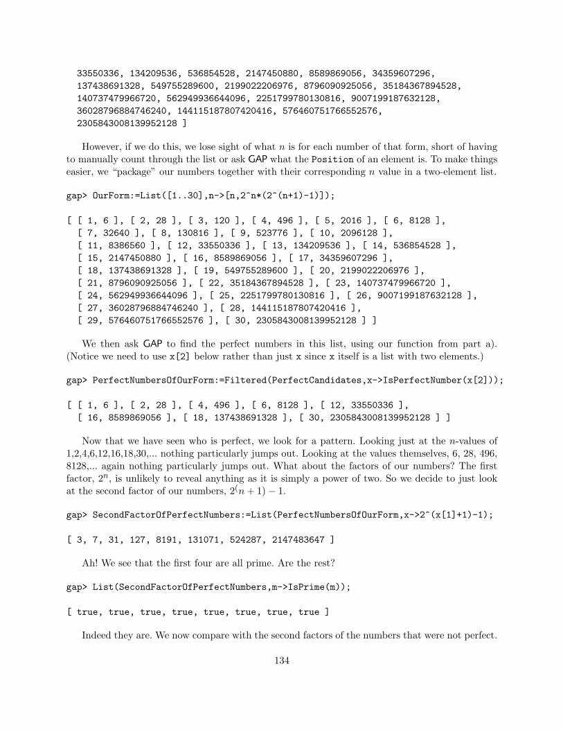
33550336, 134209536, 536854528, 2147450880, 8589869056, 34359607296,137438691328, 549755289600, 2199022206976, 8796090925056, 35184367894528,140737479966720, 562949936644096, 2251799780130816, 9007199187632128,36028796884746240, 144115187807420416, 576460751766552576,2305843008139952128 ]
However, if we do this, we lose sight of what n is for each number of that form, short of havingto manually count through the list or ask GAP what the Position of an element is. To make thingseasier, we “package” our numbers together with their corresponding n value in a two-element list.
gap> OurForm:=List([1..30],n->[n,2^n*(2^(n+1)-1)]);
[ [ 1, 6 ], [ 2, 28 ], [ 3, 120 ], [ 4, 496 ], [ 5, 2016 ], [ 6, 8128 ],[ 7, 32640 ], [ 8, 130816 ], [ 9, 523776 ], [ 10, 2096128 ],[ 11, 8386560 ], [ 12, 33550336 ], [ 13, 134209536 ], [ 14, 536854528 ],[ 15, 2147450880 ], [ 16, 8589869056 ], [ 17, 34359607296 ],[ 18, 137438691328 ], [ 19, 549755289600 ], [ 20, 2199022206976 ],[ 21, 8796090925056 ], [ 22, 35184367894528 ], [ 23, 140737479966720 ],[ 24, 562949936644096 ], [ 25, 2251799780130816 ], [ 26, 9007199187632128 ],[ 27, 36028796884746240 ], [ 28, 144115187807420416 ],[ 29, 576460751766552576 ], [ 30, 2305843008139952128 ] ]
We then ask GAP to find the perfect numbers in this list, using our function from part a).(Notice we need to use x[2] below rather than just x since x itself is a list with two elements.)
gap> PerfectNumbersOfOurForm:=Filtered(PerfectCandidates,x->IsPerfectNumber(x[2]));
[ [ 1, 6 ], [ 2, 28 ], [ 4, 496 ], [ 6, 8128 ], [ 12, 33550336 ],[ 16, 8589869056 ], [ 18, 137438691328 ], [ 30, 2305843008139952128 ] ]
Now that we have seen who is perfect, we look for a pattern. Looking just at the n-values of1,2,4,6,12,16,18,30,... nothing particularly jumps out. Looking at the values themselves, 6, 28, 496,8128,... again nothing particularly jumps out. What about the factors of our numbers? The firstfactor, 2n, is unlikely to reveal anything as it is simply a power of two. So we decide to just lookat the second factor of our numbers, 2(n+ 1)− 1.
gap> SecondFactorOfPerfectNumbers:=List(PerfectNumbersOfOurForm,x->2^(x[1]+1)-1);
[ 3, 7, 31, 127, 8191, 131071, 524287, 2147483647 ]
Ah! We see that the first four are all prime. Are the rest?
gap> List(SecondFactorOfPerfectNumbers,m->IsPrime(m));
[ true, true, true, true, true, true, true, true ]
Indeed they are. We now compare with the second factors of the numbers that were not perfect.
134

gap> NotPerfectNumbersOfOurForm:=Filtered(OurForm,x->not IsPerfectNumber(x[2]));
[ [ 3, 120 ], [ 5, 2016 ], [ 7, 32640 ], [ 8, 130816 ], [ 9, 523776 ],[ 10, 2096128 ], [ 11, 8386560 ], [ 13, 134209536 ], [ 14, 536854528 ],[ 15, 2147450880 ], [ 17, 34359607296 ], [ 19, 549755289600 ],[ 20, 2199022206976 ], [ 21, 8796090925056 ], [ 22, 35184367894528 ],[ 23, 140737479966720 ], [ 24, 562949936644096 ], [ 25, 2251799780130816 ],[ 26, 9007199187632128 ], [ 27, 36028796884746240 ],[ 28, 144115187807420416 ], [ 29, 576460751766552576 ] ]
gap> SecondFactorOfNotPerfectNumbers:=List(NotPerfectNumbersOfOurForm,x->2^(x[1]+1)-1);
[ 15, 63, 255, 511, 1023, 2047, 4095, 16383, 32767, 65535, 262143, 1048575,2097151, 4194303, 8388607, 16777215, 33554431, 67108863, 134217727,268435455, 536870911, 1073741823 ]
gap> List(SecondFactorOfNotPerfectNumbers,m->IsPrime(m));
[ false, false, false, false, false, false, false, false, false, false,false, false, false, false, false, false, false, false, false, false,false, false ]
They are all not prime. So based on this data we can make a conjecture: 2n(2n+1−1) is perfectif and only if 2n+1 − 1 is prime (in fact a Mersenne prime).
e) Assume 2n+1 − 1 is prime. Then the divisors of 2n(2n+1 − 1) are 1, 2, 22, 23, . . . , 2n and2n+1 − 1, 2(2n+1 − 1), 22(2n+1 − 1), 23(2n+1 − 1), . . . , 2n(2n+1 − 1). We can sum each of thesesequences using the formula for the sum of a finite geometric series. Thus,
(1+2+22+23+. . .+2n)+(2n+1−1)(1+2+22+23+. . .+2n) = 2n+1−1+(2n+1−1)(2n+1−1) =2n+1(2n+1 − 1)
which is exactly twice our original number.Conversley, we can see that if 2n+1 − 1 is not prime, 2n(2n+1 − 1) will have all of the divisors
listed above and more. The same computation holds, so the sum of the divisors will be strictlygreater than twice 2n(2n+1 − 1), since the sum of a proper subset is equal to it.
Exercise 2, page 60
To compute the GCD in gap we can use the command Gcd.
gap> Gcd(67458,43521);3
We can find the form axa + yb using the extended euclidean algorithm, either via ShowGcd, or asthe result of GcdRepresentation The command Gcdex(a,b) will return a useful list of information.
gap> GcdRepresentation(67458,43521);[ -4829, 7485 ]gap> ShowGcd(67458,43521);
135

67458=1*43521 + 2393743521=1*23937 + 1958423937=1*19584 + 435319584=4*4353 + 21724353=2*2172 + 92172=241*9 + 39=3*3 + 0The Gcd is 3= 1*2172 -241*9= -241*4353 + 483*2172= 483*19584 -2173*4353= -2173*23937 + 2656*19584= 2656*43521 -4829*23937= -4829*67458 + 7485*435213
Therefore we have −4829 ∗ 67458 + 7485 ∗ 43521 = 3 which we verify in GAP.
gap> -4829*67458+7485*43521;3
Exercise 3, page 61
gap> x:=X(Rationals,"x":old);;gap> f:=x^4+4*x^3-13*x^2-28*x+60;x^4+4*x^3-13*x^2-28*x+60gap> g:=x^6+5*x^5-x^4-29*x^3-12*x^2+36*x;x^6+5*x^5-x^4-29*x^3-12*x^2+36*xgap> Gcd(f,g);x^2+x-6
If use of the Gcd command is considered to simplistic, this is how to do the Euclidean algorithmby hand:
gap> a:=g;;b:=f;;gap> r:= a mod b;-20*x^3+60*x^2+200*x-480gap> a:=b;;b:=r;;gap> r:= a mod b;18*x^2+18*x-108gap> a:=b;;b:=r;;gap> r:= a mod b;0gap> b; # remainder was 0, b is the result18*x^2+18*x-108gap> 1/18*b; # scalex^2+x-6
136

Exercise 4, page 61
a) We compute the check digit using the mod command in GAP.
gap> 10*3+9*8+8*6+7*0+6*7+5*3+4*4+3*2+2*7;
243
gap> 243 mod 11;
1
Thus the check digit is X (which represents 11-1=10).b) By lowering the last digit by 4 and the second to last digit by 1, we lower our total by 11.
Thus we can change two digits and end up with the same check digit. This is verified by a similarcomputation:
gap> 10*3+9*8+8*6+7*0+6*7+5*3+4*4+3*1+2*3;
232
gap> 243 mod 11;
1
Thus the check digit is still X.
Exercise 5, page 61
To answer this question we will write a small function called Easter, which will take as input theyear and return the date. We will use the Print command to output our result. We will also usebackslash n at the end of our print command to specify a line return.
gap> Easter:=function(n)> local a, b, c, d, e;> a:=n mod 19;> b:=n mod 4;> c:=n mod 7;> d:=(19*a+24) mod 30;;> e:=(2*b+4*c+6*d+5) mod 7;> if (d+e)<10 then> Print("Easter will fall on ", d+e+22,"th March \n");> else> if not (d+e-9)=26 then> Print("Easter will fall on ", d+e-9, "th of April \n");> else> Print("Easter will fall on April 19th \n");
137
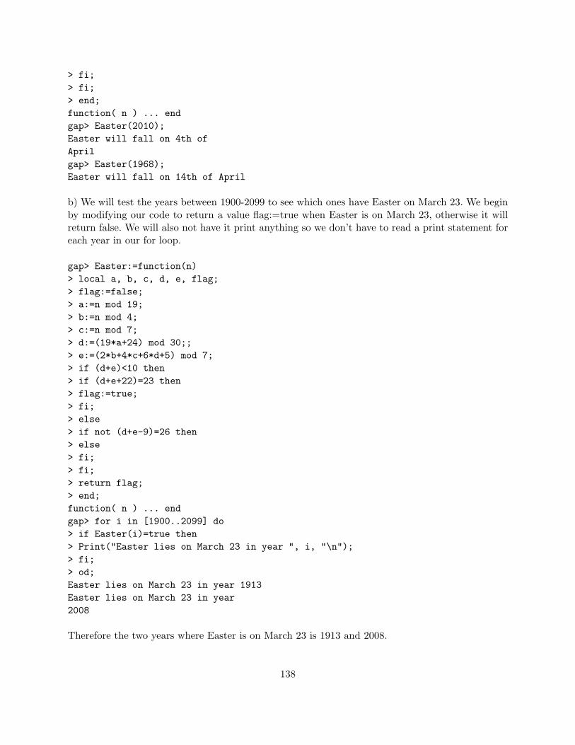
> fi;> fi;> end;function( n ) ... endgap> Easter(2010);Easter will fall on 4th ofAprilgap> Easter(1968);Easter will fall on 14th of April
b) We will test the years between 1900-2099 to see which ones have Easter on March 23. We beginby modifying our code to return a value flag:=true when Easter is on March 23, otherwise it willreturn false. We will also not have it print anything so we don’t have to read a print statement foreach year in our for loop.
gap> Easter:=function(n)> local a, b, c, d, e, flag;> flag:=false;> a:=n mod 19;> b:=n mod 4;> c:=n mod 7;> d:=(19*a+24) mod 30;;> e:=(2*b+4*c+6*d+5) mod 7;> if (d+e)<10 then> if (d+e+22)=23 then> flag:=true;> fi;> else> if not (d+e-9)=26 then> else> fi;> fi;> return flag;> end;function( n ) ... endgap> for i in [1900..2099] do> if Easter(i)=true then> Print("Easter lies on March 23 in year ", i, "\n");> fi;> od;Easter lies on March 23 in year 1913Easter lies on March 23 in year2008
Therefore the two years where Easter is on March 23 is 1913 and 2008.
138

c) We will again slightly modify our Easter code to output only a list of numbers [month,date] sowe can easily see repeats.
gap> Easter:=function(n)> local a, b, c, d, e, List;> List:=[];> a:=n mod 19;> b:=n mod 4;> c:=n mod 7;> d:=(19*a+24) mod 30;;> e:=(2*b+4*c+6*d+5) mod 7;> if (d+e)<10 then> Add(List,[3,d+e+22]);> else> if not (d+e-9)=26 then> Add(List, [4,d+e-9]);> else> Add(List, [4,19]);> fi;> fi;> return List;> end;function( n ) ... endgap> Easter(1);[ [ 4, 9 ] ]gap> Easter(2);[[ 3, 25 ] ]gap> K:=[];[ ]gap> for i in [1..100] do> Add(K,Easter(i));> od;gap> K;[ [ [ 4, 9 ] ], [ [ 3, 25 ] ], [ [ 4, 14 ] ], [ [ 4, 5 ] ],[ [ 4, 25 ] ], [ [ 4, 10 ] ], [ [ 4, 2 ] ], [ [ 4, 21 ] ],[ [ 4, 6 ] ], [ [ 3, 29 ] ], [ [ 4, 18 ] ], [ [ 4, 9 ] ], [ [ 3, 25 ] ],[ [ 4, 14 ] ], [ [ 4, 6 ] ], [ [ 4, 25 ] ],
[ [ 4, 10 ] ], [ [ 4, 2 ] ], [ [ 4, 15 ] ], [ [ 4, 6 ] ], [ [ 3, 29 ] ],[ [ 4, 18 ] ], [ [ 4, 3 ] ], [ [ 4, 22 ] ],
[ [ 4, 14 ] ], [ [ 3, 30 ] ], [ [ 4, 19 ] ], [ [ 4, 10 ] ], [ [ 3, 26 ] ],[ [ 4, 15 ] ], [ [ 4, 7 ] ], [ [ 3, 29 ] ],
[ [ 4, 11 ] ], [ [ 4, 3 ] ], [ [ 4, 23 ] ], [ [ 4, 14 ] ], [ [ 3, 30 ] ],[ [ 4, 19 ] ], [ [ 4, 4 ] ], [ [ 3, 26 ] ],
[ [ 4, 15 ] ], [ [ 4, 7 ] ], [ [ 4, 20 ] ], [ [ 4, 11 ] ], [ [ 4, 3 ] ],[ [ 4, 23 ] ], [ [ 4, 8 ] ], [ [ 3, 30 ] ],
139

[ [ 4, 19 ] ], [ [ 4, 4 ] ], [ [ 3, 27 ] ], [ [ 4, 15 ] ], [ [ 3, 31 ] ],[ [ 4, 20 ] ], [ [ 4, 12 ] ], [ [ 4, 3 ] ],[ [ 4, 16 ] ], [ [ 4, 8 ] ], [ [ 3, 24 ] ], [ [ 4, 12 ] ], [ [ 4, 4 ] ],[ [ 4, 24 ] ], [ [ 4, 9 ] ], [ [ 3, 31 ] ],
[ [ 4, 20 ] ], [ [ 4, 12 ] ], [ [ 3, 28 ] ], [ [ 4, 16 ] ], [ [ 4, 8 ] ],[ [ 3, 24 ] ], [ [ 4, 13 ] ], [ [ 4, 4 ] ],
[ [ 4, 24 ] ], [ [ 4, 9 ] ], [ [ 4, 1 ] ], [ [ 4, 20 ] ], [ [ 4, 5 ] ],[ [ 3, 28 ] ], [ [ 4, 17 ] ], [ [ 4, 1 ] ],
[ [ 4, 21 ] ], [ [ 4, 13 ] ], [ [ 3, 29 ] ], [ [ 4, 17 ] ], [ [ 4, 9 ] ],[ [ 4, 1 ] ], [ [ 4, 14 ] ], [ [ 4, 5 ] ],[ [ 3, 28 ] ], [ [ 4, 17 ] ], [ [ 4, 2 ] ], [ [ 4, 21 ] ], [ [ 4, 13 ] ],[ [ 3, 29 ] ], [ [ 4, 18 ] ], [ [ 4, 9 ] ],[ [ 3, 25 ] ], [ [ 4, 14 ] ], [ [ 4, 6 ] ], [ [ 4, 25 ] ] ]
We can see from this example that the amount of time it takes to repeat varies over time, howeversince the smallest value in March is March 22 and the largest value in April is April 25, and we donot repeat a date until a sequence has finished we know the longest we can go is 34 years beforewe cycle again.
Exercise 6, page 61
a) If g(x) = f(x) mod p(x), g(x) = f(x) + h(x)p(x) for some polynomial h(x). Thus g(α) =f(α) + h(α)p(α) = f(α) since p(α) = 0.
b) We compute mod p in GAP.
gap> x:=Indeterminate(Integers,"x");xgap> p:=x^3-6*x^2+12*x-3;x^3-6*x^2+12*x-3gap> (x-2)^3 mod p;-5
Thus we see that α = 2− 51/3.
Exercise 7, page 61
a) We enter into GAP all polynomials of degree 0 or 1.
gap> x:=Indeterminate(GF(3),"x");xgap> zero:=Zero(GF(3)); one:=One(GF(3)); two:=2*One(GF(3));0*Z(3)Z(3)^0Z(3)gap> rems:=[zero,one,two,one*x,one*x+one,one*x+two,two*x,two*x+one,two*x+two];0*Z(3), Z(3)^0, Z(3), x, x+Z(3)^0, x-Z(3)^0, -x, -x+Z(3)^0, -x-Z(3)^0 ]
b) We use a double List command to create the addition and multiplication tables.
140

gap> f:=one*x^2-two; x^2+Z(3)^0gap> multTable:=List(rems,p->List(rems,q->(q*p) mod f));[[ 0*Z(3), 0*Z(3), 0*Z(3), 0*Z(3), 0*Z(3), 0*Z(3), 0*Z(3), 0*Z(3), 0*Z(3) ],[ 0*Z(3), Z(3)^0, -Z(3)^0, x, x+Z(3)^0, x-Z(3)^0, -x, -x+Z(3)^0, -x-Z(3)^0 ],<output truncated>gap> additionTable:=List(rems,p->List(rems,q->q+p mod f));[[ 0*Z(3), Z(3)^0, -Z(3)^0, x, x+Z(3)^0, x-Z(3)^0, -x, -x+Z(3)^0, -x-Z(3)^0 ],[ Z(3)^0, -Z(3)^0, 0*Z(3), x+Z(3)^0, x-Z(3)^0, x, -x+Z(3)^0, -x-Z(3)^0, -x ],<output truncated>
Thus the tables have the property that multTable[i][j]=rems[i]*rems[j].c) Notice that the upper right-hand three-by-three corner of both tables only contains elementsfrom GF (3). Thus it is a subring.d) By trying out all three possibilities, we see it has no roots.e) Notice that x itself is a solution!f) We check that every nonzero row of the matrix has an identity (Z(0) for addition, Z(1) formultiplication) in it.
gap> Number( multTable, r -> ForAny(r,p -> p=zero*x+one));8
Exercise 8, page 62
First we get the polynomials we will quotient by as well as alpha, the image of x.
gap> x:=Indeterminate(GF(2),"x");xgap> zero:=Zero(GF(2)); one:=One(GF(2));0*Z(2)Z(2)^0gap> f:=one*x^3+one*x+one;x^3+x+Z(2)^0gap> g:=one*x^3+one*x^2+one;x^3+x^2+Z(2)^0gap> alpha:=one*x+one;x+Z(2)^0
In a few examples, we check that this respects the operations of the ring.
gap> (alpha^3+alpha+one) mod g;0*Z(2)gap> (x^2+x+1)*x mod f;x^2+Z(2)^0gap> (alpha^2+one) mod g;x^2
141

gap> (alpha^2+alpha+one)*(alpha) mod g;x^2
gap> (x^2+1)*(x+1) mod f;x^2gap> (alpha^2) mod g;x^2+Z(2)^0gap> (alpha^2+one)*(alpha+one) mod g;x^2+Z(2)^0
gap> (x^2+1)+(x+1) mod f;x^2+xgap> (alpha^2+alpha) mod g;x^2+xgap> (alpha^2+one)+(alpha+one) mod g;x^2+x
Exercise 9, page 62
Lets define the degree function first.
gap> d:=function(x) return x*ComplexConjugate(x);end;;gap> d(1+E(4));2gap> d(1+2*E(4));5
Now lets start the euclidean algorithm. We divide by the number of smaller degree, becauseotherwise the first step will just swap the variables.
gap> a:=7+E(4);; b:=-1+5*E(4);;gap> d(a);50gap> d(b);26
gap> a/b;-1/13-18/13*E(4)gap> q:=-E(4);; # we choose a gaussian integer ‘‘not too far away’’,
# rounding -1/13 to 0 and -18/13 to -1.gap> r:=a-q*b; # the reminder2gap> d(r); #indeed the degree went down.4gap> a:=b;;b:=r;; # iterategap> a/b;-1/2+5/2*E(4)
142

gap> q:=-1+2*E(4); # again we round the coefficients to get a gaussian integer-1+2*E(4)gap> r:=a-q*b;1+E(4)gap> d(r);2gap> a:=b;;b:=r;;gap> a/b;1-E(4)
At this point a/b is gaussian, this means q := a/b and r will be zero. The gcd therefore is teh lastnonzero remainder, 1 + i.
In fact GAP even has the appropriate division with remainder implemented, we could simplyask for the Gcd, rendering the problem trivial.
gap> Gcd(a,b);1+E(4)
Exercise 10, page 62
Exercise 11, page 62
gap> x:=X(Rationals,"x":old);;gap> f:=x^5+5*x^2-1;x^5+5*x^2-1gap> y:=X(GF(2),"y":old);;gap> fv:=Value(f,y);y^5+y^2+Z(2)^0gap> Factors(fv);[ y^5+y^2+Z(2)^0 ]gap> List(Factors(fv),Degree);[ 5 ]
So the first polynomial is irreducible over Z[x].
gap> f:=x^4+4*x^3+6*x^2+4*x-4;x^4+4*x^3+6*x^2+4*x-4gap> y:=X(GF(2),"y":old);;gap> fv:=Value(f,y);y^4gap> List(Factors(fv),Degree);[ 1, 1, 1, 1 ]gap> List(Factors(Value(f,X(GF(3)))),Degree);[ 2, 2 ]gap> List(Factors(Value(f,X(GF(5)))),Degree);
143
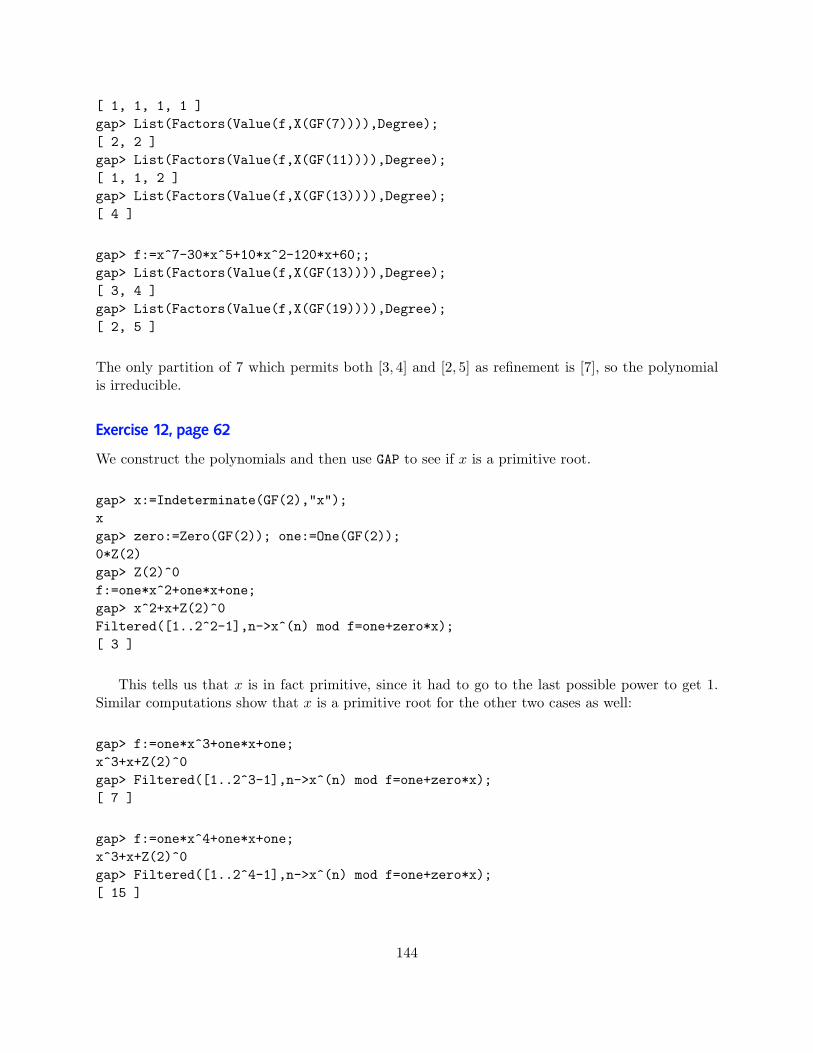
[ 1, 1, 1, 1 ]gap> List(Factors(Value(f,X(GF(7)))),Degree);[ 2, 2 ]gap> List(Factors(Value(f,X(GF(11)))),Degree);[ 1, 1, 2 ]gap> List(Factors(Value(f,X(GF(13)))),Degree);[ 4 ]
gap> f:=x^7-30*x^5+10*x^2-120*x+60;;gap> List(Factors(Value(f,X(GF(13)))),Degree);[ 3, 4 ]gap> List(Factors(Value(f,X(GF(19)))),Degree);[ 2, 5 ]
The only partition of 7 which permits both [3, 4] and [2, 5] as refinement is [7], so the polynomialis irreducible.
Exercise 12, page 62
We construct the polynomials and then use GAP to see if x is a primitive root.
gap> x:=Indeterminate(GF(2),"x");xgap> zero:=Zero(GF(2)); one:=One(GF(2));0*Z(2)gap> Z(2)^0f:=one*x^2+one*x+one;gap> x^2+x+Z(2)^0Filtered([1..2^2-1],n->x^(n) mod f=one+zero*x);[ 3 ]
This tells us that x is in fact primitive, since it had to go to the last possible power to get 1.Similar computations show that x is a primitive root for the other two cases as well:
gap> f:=one*x^3+one*x+one;x^3+x+Z(2)^0gap> Filtered([1..2^3-1],n->x^(n) mod f=one+zero*x);[ 7 ]
gap> f:=one*x^4+one*x+one;x^3+x+Z(2)^0gap> Filtered([1..2^4-1],n->x^(n) mod f=one+zero*x);[ 15 ]
144

Exercise 13, page 63
For part a), we simply see that the coefficient pi is the number of ways of adding two of theexponents together to get i as their sum. There are nm total possibilities. Thus pi/(mn) is theprobability of getting a sum of i.
For part b), we run the suggested code as above and get the following output:
gap> x:=Indeterminate(Integers,"x");xgap> dtermable:=function(f,d)f:=CoefficientsOfUnivariatePolynomial(f);return ForAll(f,i->i>=0) and Sum(f)=d;
end;function( f, d ) ... endgap> divisors:=p->List(Combinations(Factors(p)),x->Product(x,p^0));function( p ) ... endgap> p:=(x+x^2+x^3+x^4+x^5+x^6)^2;;gap> Filtered(divisors(p),i->dtermable(i,6) and Value(i,0)=0 and dtermable(p/i,6) and Value(p/i,0)=0);[ x^8+x^6+x^5+x^4+x^3+x, x^6+x^5+x^4+x^3+x^2+x, x^4+2*x^3+2*x^2+x ]
The polynomial x6 + x5 + x4 + x3 + x2 + x is the standard die. However (x8 + x6 + x5 + x4 +x3 +x)(x4 + 2 ∗x3 + 2 ∗x2 +x) = p gives us a new pair of dice that work: one is labelled 1,3,4,5,6,8and one is labelled 1,2,2,3,3,4.
We now begin part c) by investigating if it is possible for two tetrahedral dice labeled 1,2,3,4.
gap> p:=(x+x^2+x^3+x^4)^2;;gap> Filtered(divisors(p),i->dtermable(i,4) and Value(i,0)=0 and dtermable(p/i,4) and Value(p/i,0)=0);[ x^3+2*x^2+x, x^4+x^3+x^2+x, x^5+2*x^3+x ]gap> last[1]*last[3]=p;true
Thus again we have a pair of Sicherman dice! This time they are labelled 1,2,2,3 and 1,3,3,5.We now try with octahedra. Here we have enough factors that we run a Filtered command to
pluck out what pairs actually multiply to p.
gap> p:=(x+x^2+x^3+x^4+x^5+x^6+x^7+x^8)^2;;gap> dice:=Filtered(divisors(p),i->dtermable(i,8) and Value(i,0)=0 and dtermable(p/i,8) and Value(p/i,0)=0);[ x^5+2*x^4+2*x^3+2*x^2+x, x^7+2*x^6+x^5+x^3+2*x^2+x,x^6+x^5+2*x^4+2*x^3+x^2+x, x^8+x^7+x^6+x^5+x^4+x^3+x^2+x,x^10+x^9+2*x^6+2*x^5+x^2+x, x^9+2*x^7+2*x^5+2*x^3+x,x^11+x^9+2*x^7+2*x^5+x^3+x ]
gap> Filtered(Tuples(dice,2),t->t[1]*t[2]=p);[ [ x^5+2*x^4+2*x^3+2*x^2+x, x^11+x^9+2*x^7+2*x^5+x^3+x ],[ x^6+x^5+2*x^4+2*x^3+x^2+x, x^10+x^9+2*x^6+2*x^5+x^2+x ],[ x^7+2*x^6+x^5+x^3+2*x^2+x, x^9+2*x^7+2*x^5+2*x^3+x ],[ x^8+x^7+x^6+x^5+x^4+x^3+x^2+x, x^8+x^7+x^6+x^5+x^4+x^3+x^2+x ],[ x^9+2*x^7+2*x^5+2*x^3+x, x^7+2*x^6+x^5+x^3+2*x^2+x ],
145

[ x^10+x^9+2*x^6+2*x^5+x^2+x, x^6+x^5+2*x^4+2*x^3+x^2+x ],[ x^11+x^9+2*x^7+2*x^5+x^3+x, x^5+2*x^4+2*x^3+2*x^2+x ] ]
Thus we see (ignoring the original pair and duplicates on the list) we have 3 pairs of Sichermandice for the octahedron. The first is labelled 1,2,2,3,3,4,4,5 and 1,3,5,5,7,7,9,11. The second islabelled 1,2,3,3,4,4,5,6 and 1,2,5,5,6,6,9,10.
We repeat this process once more for the dodecahedron. We use a Sum command to make thecreation of p less tedious. Additionally, since we have a large number of matches at the end, we usetwo Set commands to remove duplicates from our list.
p:=(Sum([1..12],i->x^i))^2;;dice:=Filtered(divisors(p),i->dtermable(i,12) and Value(i,0)=0 and dtermable(p/i,12) and Value(p/i,0)=0);[ x^9+x^8+x^7+2*x^6+2*x^5+2*x^4+x^3+x^2+x,x^13+x^12+x^10+2*x^9+x^8+x^6+2*x^5+x^4+x^2+x,x^7+2*x^6+2*x^5+2*x^4+2*x^3+2*x^2+x,x^11+2*x^10+x^9+x^7+2*x^6+x^5+x^3+2*x^2+x,x^14+x^12+x^11+x^10+x^9+x^8+x^7+x^6+x^5+x^4+x^3+x,x^18+x^15+x^14+x^12+x^11+x^10+x^9+x^8+x^7+x^5+x^4+x,x^8+x^7+2*x^6+2*x^5+2*x^4+2*x^3+x^2+x,x^12+x^11+x^10+x^9+x^8+x^7+x^6+x^5+x^4+x^3+x^2+x,x^16+x^15+x^12+x^11+x^10+x^9+x^8+x^7+x^6+x^5+x^2+x,x^6+2*x^5+3*x^4+3*x^3+2*x^2+x, x^10+2*x^9+2*x^8+x^7+x^4+2*x^3+2*x^2+x,x^13+2*x^11+2*x^9+2*x^7+2*x^5+2*x^3+x,x^17+x^15+x^13+2*x^11+2*x^9+2*x^7+x^5+x^3+x,x^11+x^10+2*x^9+x^8+x^7+x^5+x^4+2*x^3+x^2+x,x^15+x^14+x^13+2*x^9+2*x^8+2*x^7+x^3+x^2+x ]
Filtered(Tuples(dice,2),t->t[1]*t[2]=p);[ [ x^6+2*x^5+3*x^4+3*x^3+2*x^2+x,
x^18+x^15+x^14+x^12+x^11+x^10+x^9+x^8+x^7+x^5+x^4+x ],[ x^7+2*x^6+2*x^5+2*x^4+2*x^3+2*x^2+x,
x^17+x^15+x^13+2*x^11+2*x^9+2*x^7+x^5+x^3+x ],[ x^8+x^7+2*x^6+2*x^5+2*x^4+2*x^3+x^2+x,
x^16+x^15+x^12+x^11+x^10+x^9+x^8+x^7+x^6+x^5+x^2+x ],[ x^9+x^8+x^7+2*x^6+2*x^5+2*x^4+x^3+x^2+x,
x^15+x^14+x^13+2*x^9+2*x^8+2*x^7+x^3+x^2+x ],[ x^10+2*x^9+2*x^8+x^7+x^4+2*x^3+2*x^2+x,
x^14+x^12+x^11+x^10+x^9+x^8+x^7+x^6+x^5+x^4+x^3+x ],[ x^11+x^10+2*x^9+x^8+x^7+x^5+x^4+2*x^3+x^2+x,
x^13+x^12+x^10+2*x^9+x^8+x^6+2*x^5+x^4+x^2+x ],[ x^11+2*x^10+x^9+x^7+2*x^6+x^5+x^3+2*x^2+x,
x^13+2*x^11+2*x^9+2*x^7+2*x^5+2*x^3+x ],[ x^12+x^11+x^10+x^9+x^8+x^7+x^6+x^5+x^4+x^3+x^2+x,
x^12+x^11+x^10+x^9+x^8+x^7+x^6+x^5+x^4+x^3+x^2+x ],[ x^13+2*x^11+2*x^9+2*x^7+2*x^5+2*x^3+x,
x^11+2*x^10+x^9+x^7+2*x^6+x^5+x^3+2*x^2+x ],[ x^13+x^12+x^10+2*x^9+x^8+x^6+2*x^5+x^4+x^2+x,
146

x^11+x^10+2*x^9+x^8+x^7+x^5+x^4+2*x^3+x^2+x ],[ x^14+x^12+x^11+x^10+x^9+x^8+x^7+x^6+x^5+x^4+x^3+x,
x^10+2*x^9+2*x^8+x^7+x^4+2*x^3+2*x^2+x ],[ x^15+x^14+x^13+2*x^9+2*x^8+2*x^7+x^3+x^2+x,
x^9+x^8+x^7+2*x^6+2*x^5+2*x^4+x^3+x^2+x ],[ x^16+x^15+x^12+x^11+x^10+x^9+x^8+x^7+x^6+x^5+x^2+x,
x^8+x^7+2*x^6+2*x^5+2*x^4+2*x^3+x^2+x ],[ x^17+x^15+x^13+2*x^11+2*x^9+2*x^7+x^5+x^3+x,
x^7+2*x^6+2*x^5+2*x^4+2*x^3+2*x^2+x ],[ x^18+x^15+x^14+x^12+x^11+x^10+x^9+x^8+x^7+x^5+x^4+x,
x^6+2*x^5+3*x^4+3*x^3+2*x^2+x ] ]Set(List(last,D->Set(D)));[ [ x^6+2*x^5+3*x^4+3*x^3+2*x^2+x,
x^18+x^15+x^14+x^12+x^11+x^10+x^9+x^8+x^7+x^5+x^4+x ],[ x^7+2*x^6+2*x^5+2*x^4+2*x^3+2*x^2+x,
x^17+x^15+x^13+2*x^11+2*x^9+2*x^7+x^5+x^3+x ],[ x^8+x^7+2*x^6+2*x^5+2*x^4+2*x^3+x^2+x,
x^16+x^15+x^12+x^11+x^10+x^9+x^8+x^7+x^6+x^5+x^2+x ],[ x^9+x^8+x^7+2*x^6+2*x^5+2*x^4+x^3+x^2+x,
x^15+x^14+x^13+2*x^9+2*x^8+2*x^7+x^3+x^2+x ],[ x^10+2*x^9+2*x^8+x^7+x^4+2*x^3+2*x^2+x,
x^14+x^12+x^11+x^10+x^9+x^8+x^7+x^6+x^5+x^4+x^3+x ],[ x^11+x^10+2*x^9+x^8+x^7+x^5+x^4+2*x^3+x^2+x,
x^13+x^12+x^10+2*x^9+x^8+x^6+2*x^5+x^4+x^2+x ],[ x^11+2*x^10+x^9+x^7+2*x^6+x^5+x^3+2*x^2+x,
x^13+2*x^11+2*x^9+2*x^7+2*x^5+2*x^3+x ],[ x^12+x^11+x^10+x^9+x^8+x^7+x^6+x^5+x^4+x^3+x^2+x ] ]
Thus there are 7 more pairs of Sicherman dice for dodecahedra!For part d) we repeat this process with a different p.
gap> p:=Sum([1..36],i->x^i);;dice:=Filtered(divisors(p),i->dtermable(i,6) and Value(i,0)=0 and dtermable(p/i,6) and Value(p/i,0)=0);[ ]
This shows you cannot achieve an equal probability distribution using 2 die with positive entries.We now drop the condition that all faces must be labelled positive and try again.
gap> p:=Sum([1..36],i->x^i);;gap> dice:=Filtered(divisors(p),i->dtermable(i,6) and dtermable(p/i,6));[ x^6+x^5+x^4+x^3+x^2+x, x^10+x^9+x^6+x^5+x^2+x, x^12+x^11+x^10+x^3+x^2+x,x^16+x^13+x^10+x^7+x^4+x, x^28+x^25+x^16+x^13+x^4+x,x^14+x^13+x^8+x^7+x^2+x, x^26+x^25+x^14+x^13+x^2+x, x^11+x^9+x^7+x^5+x^3+x,x^23+x^21+x^19+x^5+x^3+x, x^9+x^8+x^7+x^3+x^2+x, x^21+x^20+x^19+x^3+x^2+x,x^31+x^25+x^19+x^13+x^7+x, x^25+x^22+x^19+x^7+x^4+x,x^27+x^25+x^15+x^13+x^3+x, x^5+x^4+x^3+x^2+x+1, x^9+x^8+x^5+x^4+x+1,
147

x^11+x^10+x^9+x^2+x+1, x^15+x^12+x^9+x^6+x^3+1, x^27+x^24+x^15+x^12+x^3+1,x^13+x^12+x^7+x^6+x+1, x^25+x^24+x^13+x^12+x+1, x^10+x^8+x^6+x^4+x^2+1,x^22+x^20+x^18+x^4+x^2+1, x^8+x^7+x^6+x^2+x+1, x^20+x^19+x^18+x^2+x+1,x^30+x^24+x^18+x^12+x^6+1, x^24+x^21+x^18+x^6+x^3+1,x^26+x^24+x^14+x^12+x^2+1 ]
gap> p/last[1];x^30+x^24+x^18+x^12+x^6+1
Thus for example one pair of dice that would give you the even probability distribution would beone standard six-sided die and the other with labels 0,6,12,18,24,30. We now use similar reasoningto show that there are none for octahedra or dodecahedra.
gap> dice:=Filtered(divisors(p),i->dtermable(i,8) and dtermable(p/i,8));[ ]gap> dice:=Filtered(divisors(p),i->dtermable(i,12) and dtermable(p/i,12));[ ]
For part e), we investigate using the same methods and find that there are no possibilities otherthan three standard die or one standard die with a pair of Sicherman dice.
gap> p:=(x+x^2+x^3+x^4+x^5+x^6)^3;;gap> dtermDivs:=Filtered(divisors(p),i->dtermable(i,6) and Value(i,0)=0);[ x^10+x^8+x^7+x^6+x^5+x^3, x^8+x^7+x^6+x^5+x^4+x^3, x^6+2*x^5+2*x^4+x^3,x^9+x^7+x^6+x^5+x^4+x^2, x^7+x^6+x^5+x^4+x^3+x^2, x^5+2*x^4+2*x^3+x^2,x^8+x^6+x^5+x^4+x^3+x, x^6+x^5+x^4+x^3+x^2+x, x^4+2*x^3+2*x^2+x ]
gap> Filtered(Tuples(dtermDivs,3),t->Product(t)=p);[ [ x^4+2*x^3+2*x^2+x, x^6+x^5+x^4+x^3+x^2+x, x^8+x^6+x^5+x^4+x^3+x ],[ x^4+2*x^3+2*x^2+x, x^8+x^6+x^5+x^4+x^3+x, x^6+x^5+x^4+x^3+x^2+x ],[ x^6+x^5+x^4+x^3+x^2+x, x^4+2*x^3+2*x^2+x, x^8+x^6+x^5+x^4+x^3+x ],[ x^6+x^5+x^4+x^3+x^2+x, x^6+x^5+x^4+x^3+x^2+x, x^6+x^5+x^4+x^3+x^2+x ],[ x^6+x^5+x^4+x^3+x^2+x, x^8+x^6+x^5+x^4+x^3+x, x^4+2*x^3+2*x^2+x ],[ x^8+x^6+x^5+x^4+x^3+x, x^4+2*x^3+2*x^2+x, x^6+x^5+x^4+x^3+x^2+x ],[ x^8+x^6+x^5+x^4+x^3+x, x^6+x^5+x^4+x^3+x^2+x, x^4+2*x^3+2*x^2+x ] ]
However once again if we allow zeros on our dice, we do get many solutions.
gap> p:=(x+x^2+x^3+x^4+x^5+x^6)^3;;gap> dtermDivs:=Filtered(divisors(p),i->dtermable(i,6));[ x^10+x^8+x^7+x^6+x^5+x^3, x^8+x^7+x^6+x^5+x^4+x^3, x^6+2*x^5+2*x^4+x^3,x^9+x^7+x^6+x^5+x^4+x^2, x^7+x^6+x^5+x^4+x^3+x^2, x^5+2*x^4+2*x^3+x^2,x^8+x^6+x^5+x^4+x^3+x, x^6+x^5+x^4+x^3+x^2+x, x^4+2*x^3+2*x^2+x,x^7+x^5+x^4+x^3+x^2+1, x^5+x^4+x^3+x^2+x+1, x^3+2*x^2+2*x+1 ]
gap> Filtered(Tuples(dtermDivs,3),t->Product(t)=p);[ [ x^3+2*x^2+2*x+1, x^5+x^4+x^3+x^2+x+1, x^10+x^8+x^7+x^6+x^5+x^3 ],[ x^3+2*x^2+2*x+1, x^6+x^5+x^4+x^3+x^2+x, x^9+x^7+x^6+x^5+x^4+x^2 ],[ x^3+2*x^2+2*x+1, x^7+x^5+x^4+x^3+x^2+1, x^8+x^7+x^6+x^5+x^4+x^3 ],
148

[ x^3+2*x^2+2*x+1, x^7+x^6+x^5+x^4+x^3+x^2, x^8+x^6+x^5+x^4+x^3+x ],...
Exercise 14, page 64
For c) part 1, we get that the polynomial is irreducible mod 2, and thus is irreducible.
gap> x:=X(Rationals,"x");;gap> f:=x^5+5*x^2-1;x^5+5*x^2-1gap> r:=Integers mod 2;GF(2)gap> y:=X(r);x_1gap> fr:=Value(f,y);x_1^5+x_1^2+Z(2)^0gap> List(Factors(fr),Degree);[ 5 ]
We try the same trick for the second polynomial.
x:=X(Rationals,"x");;f:=x^4+4*x^3+6*x^2+4*x-4;x^4+4*x^3+6*x^2+4*x-4r:=Integers mod 2;GF(2)y:=X(r);x_1fr:=Value(f,y);x_1^4List(Factors(fr),Degree);[ 1, 1, 1, 1 ]
However, this degree distribution tells us essentially nothing about the factorization of theoriginal polynomial. Thus we try using a different ideal.
x:=X(Rationals,"x");;f:=x^4+4*x^3+6*x^2+4*x-4;x^4+4*x^3+6*x^2+4*x-4r:=Integers mod 3;GF(3)y:=X(r);xfr:=Value(f,y);x^4+x^3+x-Z(3)^0List(Factors(fr),Degree);[ 2, 2 ]
149

We now see the polynomial is either irreducible or splits into a product of two quadratic terms.We try another ideal to see if we can rule out the product of two quadratics. It turns out 13 doesthe trick.
x:=X(Rationals,"x");;f:=x^4+4*x^3+6*x^2+4*x-4;x^4+4*x^3+6*x^2+4*x-4r:=Integers mod 13;GF(13)y:=X(r);x_1fr:=Value(f,y);x_1^4+Z(13)^2*x_1^3+Z(13)^5*x_1^2+Z(13)^2*x_1+Z(13)^8List(Factors(fr),Degree);[ 4 ]
Thus x4 + 4 ∗x3 + 6 ∗x2 + 4 ∗x− 4 is irreducible as well. We now do the third polynomial. Herewe find two different splits that can only refine a trivial partition, thus giving us irreducibility ofx7 − 30 ∗ x5 + 10 ∗ x2 − 120 ∗ x− 60.
gap> x:=X(Rationals,"x");;gap> f:=x^7-30*x^5+10*x^2-120*x-60;x^7-30*x^5+10*x^2-120*x-60gap> r:=Integers mod 7;GF(7)gap> y:=X(r);x_1gap> fr:=Value(f,y);x_1^7+Z(7)^5*x_1^5+Z(7)*x_1^2-x_1+Z(7)gap> List(Factors(fr),Degree);[ 1, 6 ]gap> r:=Integers mod 17;GF(17)gap> y:=X(r);x_1gap> fr:=Value(f,y);x_1^7+Z(17)^12*x_1^5+Z(17)^3*x_1^2-x_1+Z(17)^10gap> List(Factors(fr),Degree);[ 2, 2, 3 ]
Exercise 15, page 64
We will use the command Resultant which takes as input two polynomials and an indeterminant(x) which is one unknown quantity. This command returns a polynomial which is the product∏
(x,y):P (x)=0,Q(y)=0(x − y). We then use the command Factors(polynomial) which list all of thepossible factors. The roots of these factors are the y-values of the intersection of the two curves.
150

For each of these y-values we then plug back into the original polynomials to get polynomials inonly x. We again use factors to find the x-values that correspond to each y-value in the solutions.
gap> x:=X(Rationals,"x");xgap> y:=X(Rationals,"y");ygap>p:=x^2*y-3*x*y^2+x^2-3*x*y; x^2*y-3*x*y^2+x^2-3*x*ygap>q:=x^3*y+x^3-4*y^2-3*y+1; x^3*y+x^3-4*y^2-3*y+1gap>f:=Resultant(p,q,x);-108*y^9-513*y^8-929*y^7-738*y^6-149*y^5+112*y^4+37*y^3-14*y^2-3*y+1gap> Factors(f);[ -108*y+27, y+1, y+1, y+1, y+1, y+1,y^3-4/27*y+1/27 ]gap> #Now setting each factor each to zero we canfind solutions in terms of xgap> y:=-27/-108;1/4gap>p:=x^2*y-3*x*y^2+x^2-3*x*y; 5/4*x^2-15/16*xgap> Factors(p);[5/4*x-15/16, x ]gap> (15/16)/(5/4);3/4gap> #So we have solutions(0,1/4), (3/4,1/4)gap> y:=-1;-1gap> p:=x^2*y-3*x*y^2+x^2-3*x*y;0gap> q:=x^3*y+x^3-4*y^2-3*y+1;0gap> #Therefore we have solutionsy=-1gap> #The last polynomial does not have rational roots
Hence the rational solutions to this system consists of the pairs (0,1/4), (3/4,1/4) and y=-1.
Exercise 16, page 64
a) Using the equations x = r · cos(θ), y = r · sin(θ) we get x = (1 + cos(2θ)) cos(θ) and y =(1 + cos(2θ)) sin(θ).
151

b) We now use the double angle formula cos(2θ) = 2 cos2(θ) − 1 and get x = (1 + 2 cos2(θ) −1) cos(θ) = 2 · w3 and y = (1 + 2 cos2(θ)− 1) sin(θ) = 2 · w2z.
c) The polynomials are from b) x− 2w3, y − 2w2z as well as z2 + w2 − 1. We now calculate aGroebner basis with lex ordering with z > w > x > y, this will eliminate z and w if possible.
gap> x:=X(Rationals,"x");;gap> y:=X(Rationals,"y");;gap> z:=X(Rationals,"z");;gap> w:=X(Rationals,"w");;gap> pols:=[x-2*w^3,y-2*w^2*z,z^2+w^2-1];[ -2*w^3+x, -2*z*w^2+y, z^2+w^2-1 ]gap> bas:=ReducedGroebnerBasis(pols,MonomialLexOrdering(z,w,x,y));[ x^6+3*x^4*y^2+3*x^2*y^4+y^6-4*x^4, 1/2*x^5+3/2*x^3*y^2+x*y^4+y^4*w-2*x^3,-1/2*x^2+x*w-1/2*y^2, 1/4*x^4+1/2*x^2*y^2+1/4*y^4+y^2*w^2-x^2, w^3-1/2*x,1/2*x^2+1/2*y^2+y*z-2*w^2, x*z-y*w, z*w^2-1/2*y, z^2+w^2-1 ]
The first element in bas is the only polynomial not involving z and w, it thus is a polynomialdefining the curve. This polynomial does not factor, however the part without the last term does.
gap> curve+4*x^4;x^6+3*x^4*y^2+3*x^2*y^4+y^6gap> Collected(Factors(curve+4*x^4));[ [ x^2+y^2, 3 ] ]
So the curve is defined by (x2 + y2)3 = 4x4.
Exercise 17, page 64
We declare our indeterminates and then use the built-in command ReducedGroebnerBasis and thebuilt-in monomial orderings MonomialLexOrdering and MonomialGrlexOrdering.
gap> x:=Indeterminate(Rationals,"x");xgap> y:=Indeterminate(Rationals,"y");ygap> z:=Indeterminate(Rationals,"z");zgap> f:=x^5+y^4+z^3-1;x^5+y^4+z^3-1gap> g:=x^3+y^2+z^2-1;x^3+y^2+z^2-1gap> I:=[f,g];[ x^5+y^4+z^3-1, x^3+y^2+z^2-1 ]gap> Size(ReducedGroebnerBasis(I,MonomialLexOrdering()));7gap> Size(ReducedGroebnerBasis(I,MonomialGrlexOrdering()));5
152

We repeat the process, and notice this time one basis got larger while the other got smaller!Additionally, the polynomials in the Lex basis are enormous compared to the ones in the Grlexbasis (not shown here as the output is huge).
gap> f:=x^5+y^4+z^3-1;x^5+y^4+z^3-1gap> g:=x^3+y^3+z^2-1;x^3+y^3+z^2-1gap> I:=[f,g];[ x^5+y^4+z^3-1, x^3+y^3+z^2-1 ]gap> Size(ReducedGroebnerBasis(I,MonomialLexOrdering()));8gap> Size(ReducedGroebnerBasis(I,MonomialGrlexOrdering()));3
Exercise 18, page 65
We compute a Groebner basis but add a “fake” variable a and the relation x ∗ a− 1 to create a asthe inverse of x. Then we use Groebner bases to solve for a in terms of the other variables.
gap> x:=Indeterminate(Rationals,"x");xgap> y:=Indeterminate(Rationals,"y");ygap> z:=Indeterminate(Rationals,"z");zgap> a:=Indeterminate(Rationals,"a");agap> f:=x^2+y*z-2;x^2+y*z-2gap> g:=y^2+x*z-3;x*z+y^2-3gap> h:=x*y+z^2-5;x*y+z^2-5gap> I:=[f,g,h];[ x^2+y*z-2, x*z+y^2-3, x*y+z^2-5 ]gap> B:=ReducedGroebnerBasis(I,MonomialLexOrdering());[ z^8-25/2*z^6+219/4*z^4-95*z^2+361/8,8/361*z^7+52/361*z^5-740/361*z^3+y+75/19*z,-88/361*z^7+872/361*z^5-2690/361*z^3+x+125/19*z ]
gap> C:=ReducedGroebnerBasis(Union(B,[x*a-1]),MonomialLexOrdering([a,x,y,z]));[ z^8-25/2*z^6+219/4*z^4-95*z^2+361/8,8/361*z^7+52/361*z^5-740/361*z^3+y+75/19*z,-88/361*z^7+872/361*z^5-2690/361*z^3+x+125/19*z,200/3971*z^7-1588/3971*z^5+2438/3971*z^3+a+70/209*z ]
153

Thus we see from the final relation that the inverse of x must be equal to −200/3971 ∗ z7 +1588/3971 ∗ z5 − 2438/3971 ∗ z3 − 70/209 ∗ z. We multiply by x and reduce just to check.
gap> xinv:=-(200/3971*z^7-1588/3971*z^5+2438/3971*z^3+70/209*z);-200/3971*z^7+1588/3971*z^5-2438/3971*z^3-70/209*zgap> PolynomialReducedRemainder(x*xinv,B,MonomialLexOrdering());1
Exercise 19, page 65
Using symmetry as suggested, we have that our one perpendicular bisector is the line x = 1/2. Thuswe simply write down equations for the other two perpendicular bisectors in terms of C = (c1, c2)and show that they intersect when x = 1/2.
gap> x:=Indeterminate(Rationals,"x");xgap> y:=Indeterminate(Rationals,"y");ygap> c1:=Indeterminate(Rationals,"c1");c1gap> c2:=Indeterminate(Rationals,"c2");c2gap> f:=c2*y-c2^2/2+c1*(x-c1/2);x*c1+y*c2-1/2*c1^2-1/2*c2^2gap> g:=c2*y-c2^2/2+(c1-1)*(x-(1+c1)/2);x*c1+y*c2-1/2*c1^2-1/2*c2^2-x+1/2gap> I:=[f,g];[ x*c1+y*c2-1/2*c1^2-1/2*c2^2, x*c1+y*c2-1/2*c1^2-1/2*c2^2-x+1/2 ]gap> B:=ReducedGroebnerBasis(I,MonomialLexOrdering());[ y*c2-1/2*c1^2-1/2*c2^2+1/2*c1, x-1/2 ]
Exercise 20, page 65
We work over the quotient field of the ring Q[a, b, c, d, e, f ] and denote the coordinates of the centerby (x, y). Then the circle is described by the following polynomial equations.
(a− x)2 + (d− y)2 = (b− x)2 + (e− y)2 = (c− x)2 + (f − y)2.
The ideal generated by these polynomials must contain polynomials of degree 1 that express x andy. A Groebner basis with respect to degree must find these
gap> bas:=PolynomialRing(Rationals,["a","b","c","d","e","f"]);Rationals[a,b,c,d,e,f]gap> AssignGeneratorVariables(bas);#I Assigned the global variables [ a, b, c, d, e, f ]gap> x:=X(bas,"x");
154

#I You are creating a polynomial *over* a polynomial ring (i.e. in an#I iterated polynomial ring). Are you sure you want to do this?#I If not, the first argument should be the base ring, not a polynomial ring#I Set ITER_POLY_WARN:=false; to remove this warning.xgap> y:=X(bas,"y");#I You are creating a polynomial *over* a polynomial ring (i.e. in an#I iterated polynomial ring). Are you sure you want to do this?#I If not, the first argument should be the base ring, not a polynomial ring#I Set ITER_POLY_WARN:=false; to remove this warning.ygap> l:=[(a-x)^2+(d-y)^2-(b-x)^2-(e-y)^2,(b-x)^2+(e-y)^2-(c-x)^2-(f-y)^2];[ (-2*a+2*b)*x+(-2*d+2*e)*y+(a^2-b^2+d^2-e^2),(-2*b+2*c)*x+(-2*e+2*f)*y+(b^2-c^2+e^2-f^2) ]
gap> gb:=ReducedGroebnerBasis(l,MonomialGrlexOrdering());[ y+((2*a^2*b-2*a^2*c-2*a*b^2+2*a*c^2-2*a*e^2+2*a*f^2+2*b^2*c-2*b*c^2+2*b*d^2
-2*b*f^2-2*c*d^2+2*c*e^2)/(4*a*e-4*a*f-4*b*d+4*b*f+4*c*d-4*c*e)),x+((-2*a^2*e+2*a^2*f+2*b^2*d-2*b^2*f-2*c^2*d+2*c^2*e-2*d^2*e+2*d^2*f
+2*d*e^2-2*d*f^2-2*e^2*f+2*e*f^2)/(4*a*e-4*a*f-4*b*d+4*b*f+4*c*d-4*c*e)) ]
We conclude that with z = 2(ae− af − bd+ bf + cd− ce) we get that
x =a2e− a2f − b2d+ b2f + c2d− c2e+ d2e− d2f − de2 + df2 + e2f − ef2
z
y = −a2b− a2c− ab2 + ac2 − ae2 + af2 + b2c− bc2 + bd2 − bf2 − cd2 + ce2
z
Exercise 21, page 65
Here we use the fact that the lcm of f and g is just the t-free polynomial in the Groebner basis for< tf, (1− t)g >.
gap> x:=Indeterminate(Rationals,"x");xgap> y:=Indeterminate(Rationals,"y");ygap> z:=Indeterminate(Rationals,"z");zgap> t:=Indeterminate(Rationals,"t");tgap> f:=x^3*z^2+x^2*y*z^2-y^3*z^2+x^4+x^3*y-x^2*y^2-x*y^3;x^3*z^2+x^2*y*z^2-y^3*z^2+x^4+x^3*y-x^2*y^2-x*y^3gap> g:=x^2*z^4-y^2*z^4+2*x^3*z^2-2*x*y^2*z^2+x^4-x^2*y^2;x^2*z^4-y^2*z^4+2*x^3*z^2-2*x*y^2*z^2+x^4-x^2*y^2gap> I:=[t*f,(1-t)*g];
155

[ x^3*z^2*t+x^2*y*z^2*t-y^3*z^2*t+x^4*t+x^3*y*t-x^2*y^2*t-x*y^3*t,-x^2*z^4*t+y^2*z^4*t-2*x^3*z^2*t+x^2*z^4+2*x*y^2*z^2*t-y^2*z^4-x^4*t+2*x^3*z\
^2+x^2*y^2*t-2*x*y^2*z^2+x^4-x^2*y^2 ]gap> B:=ReducedGroebnerBasis(I,MonomialLexOrdering([t,x,y,z]));[ x^5*z^6+x^4*y*z^6-x^3*y^2*z^6-2*x^2*y^3*z^6+y^5*z^6+3*x^6*z^4+3*x^5*y*z^4-4*\x^4*y^2*z^4-6*x^3*y^3*z^4+x^2*y^4*z^4+3*x*y^5*z^4+3*x^7*z^2+3*x^6*y*z^2-5*x^5*\y^2*z^2-6*x^4*y^3*z^2+2*x^3*y^4*z^2+3*x^2*y^5*z^2+x^8+x^7*y-2*x^6*y^2-2*x^5*y^\3+x^4*y^4+x^3*y^5,y^4*z^8*t+x^4*z^8+x^3*y*z^8-x*y^3*z^8-y^4*z^8+4*x^5*z^6+4*x^4*y*z^6-4*x^3*y^\
2*z^6-7*x^2*y^3*z^6+3*y^5*z^6+5*x^6*z^4+4*x^5*y*z^4-9*x^4*y^2*z^4-9*x^3*y^3*z^\4+5*x^2*y^4*z^4+5*x*y^5*z^4-y^6*z^4+2*x^7*z^2-6*x^5*y^2*z^2-x^4*y^3*z^2+6*x^3*\y^4*z^2+x^2*y^5*z^2-2*x*y^6*z^2-x^7*y-x^6*y^2+2*x^5*y^3+2*x^4*y^4-x^3*y^5-x^2*\y^6,y^4*z^6*t+x^4*z^6+x^3*y*z^6+x*y^4*z^4*t-x*y^3*z^6-y^4*z^6+3*x^5*z^4+3*x^4*y*\
z^4-2*x^3*y^2*z^4-4*x^2*y^3*z^4-x*y^4*z^4+y^5*z^4+3*x^6*z^2+3*x^5*y*z^2-4*x^4*\y^2*z^2-5*x^3*y^3*z^2+x^2*y^4*z^2+2*x*y^5*z^2+x^7+x^6*y-2*x^5*y^2-2*x^4*y^3+x^\3*y^4+x^2*y^5,y^4*z^6*t+x^4*z^6+x^3*y*z^6-x*y^3*z^6+y^5*z^4*t-y^4*z^6+4*x^5*z^4+5*x^4*y*z^\
4-3*x^3*y^2*z^4-7*x^2*y^3*z^4+x*y^5*z^2*t-x*y^4*z^4+2*y^5*z^4+5*x^6*z^2+7*x^5*\y*z^2-6*x^4*y^2*z^2-11*x^3*y^3*z^2+x^2*y^4*z^2+4*x*y^5*z^2+2*x^7+3*x^6*y-3*x^5\*y^2-5*x^4*y^3+x^3*y^4+2*x^2*y^5,x*y^2*z^4*t+x^3*z^4+x^2*y^2*z^2*t+x^2*y*z^4-x*y^2*z^4-y^3*z^4+2*x^4*z^2+2*x^\
3*y*z^2-2*x^2*y^2*z^2-2*x*y^3*z^2+x^5+x^4*y-x^3*y^2-x^2*y^3,x^2*z^8*t-y^2*z^8*t+x^3*z^6*t-x^2*z^8-2*x*y^2*z^6*t+y^2*z^8-2*x^3*z^6-x^2*y*\
z^6-x*y^3*z^4*t+2*x*y^2*z^6+y^4*z^4*t+y^3*z^6-x^3*y*z^4+x*y^4*z^2*t+x*y^3*z^4+\2*x^5*z^2+x^4*y*z^2-2*x^3*y^2*z^2-x^2*y^3*z^2+x^6+x^5*y-x^4*y^2-x^3*y^3,-x^2*z^4*t+y^2*z^4*t-x^3*z^2*t+x^2*y*z^2*t+x^2*z^4+2*x*y^2*z^2*t-y^3*z^2*t-y\
^2*z^4+x^3*y*t+2*x^3*z^2-x*y^3*t-2*x*y^2*z^2+x^4-x^2*y^2,x^2*z^4*t-y^2*z^4*t+2*x^3*z^2*t-x^2*z^4-2*x*y^2*z^2*t+y^2*z^4+x^4*t-2*x^3*z^\
2-x^2*y^2*t+2*x*y^2*z^2-x^4+x^2*y^2 ]gap> lcm:=last[1];x^5*z^6+x^4*y*z^6-x^3*y^2*z^6-2*x^2*y^3*z^6+y^5*z^6+3*x^6*z^4+3*x^5*y*z^4-4*x^\4*y^2*z^4-6*x^3*y^3*z^4+x^2*y^4*z^4+3*x*y^5*z^4+3*x^7*z^2+3*x^6*y*z^2-5*x^5*y^\2*z^2-6*x^4*y^3*z^2+2*x^3*y^4*z^2+3*x^2*y^5*z^2+x^8+x^7*y-2*x^6*y^2-2*x^5*y^3+\x^4*y^4+x^3*y^5
We then can compute the gcd by using the formula gcd(f, g) ∗ lcm(f, g) = f ∗ g.
gap> f*g/lcm;1
Exercise 22, page 102
The group of symmetries of an equilateral triangle triangle is D6 = S3 Therefore we can use themultiplication table for S3. We will use the command SymmetricGroup to get our group, and then
156
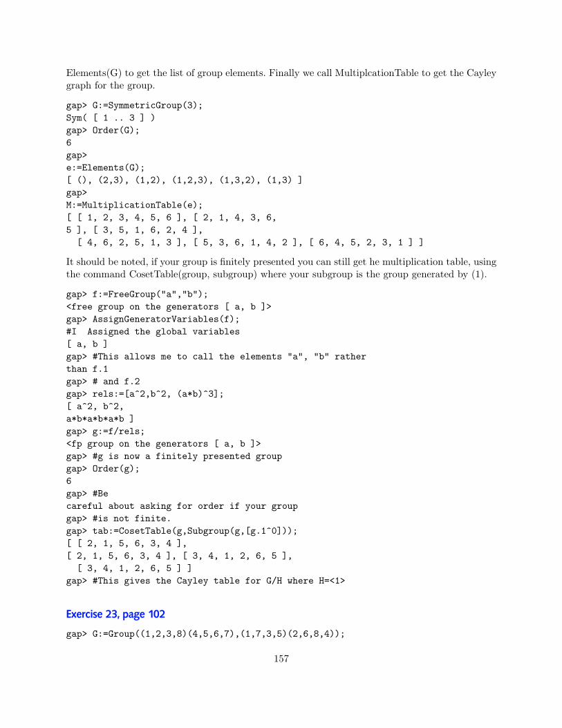
Elements(G) to get the list of group elements. Finally we call MultiplcationTable to get the Cayleygraph for the group.
gap> G:=SymmetricGroup(3);Sym( [ 1 .. 3 ] )gap> Order(G);6gap>e:=Elements(G);[ (), (2,3), (1,2), (1,2,3), (1,3,2), (1,3) ]gap>M:=MultiplicationTable(e);[ [ 1, 2, 3, 4, 5, 6 ], [ 2, 1, 4, 3, 6,5 ], [ 3, 5, 1, 6, 2, 4 ],[ 4, 6, 2, 5, 1, 3 ], [ 5, 3, 6, 1, 4, 2 ], [ 6, 4, 5, 2, 3, 1 ] ]
It should be noted, if your group is finitely presented you can still get he multiplication table, usingthe command CosetTable(group, subgroup) where your subgroup is the group generated by (1).
gap> f:=FreeGroup("a","b");<free group on the generators [ a, b ]>gap> AssignGeneratorVariables(f);#I Assigned the global variables[ a, b ]gap> #This allows me to call the elements "a", "b" ratherthan f.1gap> # and f.2gap> rels:=[a^2,b^2, (a*b)^3];[ a^2, b^2,a*b*a*b*a*b ]gap> g:=f/rels;<fp group on the generators [ a, b ]>gap> #g is now a finitely presented groupgap> Order(g);6gap> #Becareful about asking for order if your groupgap> #is not finite.gap> tab:=CosetTable(g,Subgroup(g,[g.1^0]));[ [ 2, 1, 5, 6, 3, 4 ],[ 2, 1, 5, 6, 3, 4 ], [ 3, 4, 1, 2, 6, 5 ],[ 3, 4, 1, 2, 6, 5 ] ]
gap> #This gives the Cayley table for G/H where H=<1>
Exercise 23, page 102
gap> G:=Group((1,2,3,8)(4,5,6,7),(1,7,3,5)(2,6,8,4));
157

Group([ (1,2,3,8)(4,5,6,7), (1,7,3,5)(2,6,8,4) ])gap> Elements(G);[ (), (1,2,3,8)(4,5,6,7), (1,3)(2,8)(4,6)(5,7), (1,4,3,6)(2,7,8,5),(1,5,3,7)(2,4,8,6), (1,6,3,4)(2,5,8,7), (1,7,3,5)(2,6,8,4),(1,8,3,2)(4,7,6,5) ]
gap> Size(G);8
Exercise 24, page 103
Exercise 25, page 103
Exercise 27, page 104
We construct the group and look at the sizes of the subgroups.
gap> G:=Group((1,2,3),(2,3,4));Group([ (1,2,3), (2,3,4) ])gap> s:=Union(List(ConjugacyClassesSubgroups(G),Elements));[ Group(()), Group([ (2,4,3) ]), Group([ (1,3)(2,4), (1,2)(3,4), (2,4,3) ]),Group([ (1,2)(3,4) ]), Group([ (1,3)(2,4), (1,2)(3,4) ]),Group([ (1,2,3) ]), Group([ (1,4,2) ]), Group([ (1,3,4) ]),Group([ (1,3)(2,4) ]), Group([ (1,4)(2,3) ]) ]gap> List(s,Size);[ 1, 3, 12, 2, 4, 3, 3, 3, 2, 2 ]
For drawing the subgroup lattice, we would like to get the subgroups somewhat more in order.So we sort them by size and then call a double List command to create an incidence matrix fromwhich the lattice can easily be drawn.
gap> Sort(s,function(v,w) return Size(v)<Size(w); end);gap> List(s,i->List(s,j->IsSubset(j,i)));[ [ true, true, true, true, true, true, true, true, true, true ],[ false, true, false, false, false, false, false, false, true, true ],[ false, false, true, false, false, false, false, false, true, true ],[ false, false, false, true, false, false, false, false, true, true ],[ false, false, false, false, true, false, false, false, false, true ],[ false, false, false, false, false, true, false, false, false, true ],[ false, false, false, false, false, false, true, false, false, true ],[ false, false, false, false, false, false, false, true, false, true ],[ false, false, false, false, false, false, false, false, true, true ],[ false, false, false, false, false, false, false, false, false, true ] ]
Finally, the command Filtered gives us the cyclic and normal subgroups.
158

gap> Filtered(s,IsCyclic);[ Group(()), Group([ (1,2)(3,4) ]), Group([ (1,3)(2,4) ]),Group([ (1,4)(2,3) ]), Group([ (2,4,3) ]), Group([ (1,2,3) ]),Group([ (1,4,2) ]), Group([ (1,3,4) ]) ]gap> Filtered(s,H->IsNormal(G,H));[ Group(()), Group([ (1,3)(2,4), (1,2)(3,4) ]),Group([ (1,3)(2,4), (1,2)(3,4), (2,4,3) ]) ]
Exercise 28, page 105
a) Follows easily from basic properties of groups.For b), we enter the group G and then use the command Action to define a new action of G.
gap> G:=Group((1,2,3,4),(1,3));Group([ (1,2,3,4), (1,3) ])gap> Size(G);8gap> tups:=Tuples([1..4],2);[ [ 1, 1 ], [ 1, 2 ], [ 1, 3 ], [ 1, 4 ], [ 2, 1 ], [ 2, 2 ], [ 2, 3 ],[ 2, 4 ], [ 3, 1 ], [ 3, 2 ], [ 3, 3 ], [ 3, 4 ], [ 4, 1 ], [ 4, 2 ],[ 4, 3 ], [ 4, 4 ] ]
gap> sets:=Set(tups,T->Set(T));[ [ 1 ], [ 1, 2 ], [ 1, 3 ], [ 1, 4 ], [ 2 ], [ 2, 3 ], [ 2, 4 ], [ 3 ],[ 3, 4 ], [ 4 ] ]
gap> sets:=Filtered(sets,S->Size(S)=2);[ [ 1, 2 ], [ 1, 3 ], [ 1, 4 ], [ 2, 3 ], [ 2, 4 ], [ 3, 4 ] ]gap> Action(G,sets,OnSets);Group([ (1,4,6,3)(2,5), (1,4)(3,6) ])
Exercise 29, page 105
We label the faces of the dodecahedron and then write down A, B, and C as permutations on 12points.
gap> A:=(2,3,4,5,6)(7,8,9,10,11);(2,3,4,5,6)(7,8,9,10,11)gap> B:=(1,2,3)(4,6,8)(5,7,9)(10,11,12);(1,2,3)(4,6,8)(5,7,9)(10,11,12)gap> C:=(1,2)(3,6)(4,7)(5,8)(9,11)(10,12);(1,2)(3,6)(4,7)(5,8)(9,11)(10,12)
Thus < A > has 4 orbits and should fix 24 colorings (choosing a solid color for each orbit).Similarly, < B > has 4 orbits and should fix 24 colorings. Finally, < C > has 6 orbits and shouldfix 26 colorings. The identity clearly fixes all 212 colorings.
159

Applying the Cauchy-Frobenius-Burnside Lemma, we get that the number of distinct coloringsis the average number of fixed points of all group elements:
gap> 1/60*(1*2^12+24*16+20*16+15*64);96
Thus there are 96 different ways to color the dodecahedron with green and gold.Note that we can easily use GAP to check how many fixed points there are for the different types
of elements by letting the permutations act on 12-tuples of colors (here the colors are representedby 0 and 1).
gap> colorings:=Cartesian(List([1..12],x->[0,1]));;gap> colorings[3];[ 0, 0, 0, 0, 0, 0, 0, 0, 0, 0, 1, 0 ]gap> List([1..12],j->colorings[3][j^A]);[ 0, 0, 0, 0, 0, 0, 0, 0, 0, 1, 0, 0 ]gap> Number(colorings,col->List([1..12],j->col[j^A])=col);16gap> Number(colorings,col->List([1..12],j->col[j^B])=col);16gap> Number(colorings,col->List([1..12],j->col[j^C])=col);64
Exercise 30, page 106
a) With thegroup as defined, we have to be careful to move the cubie 16/19/24 in its right position.
With this, we get the following unfolded diagram:
8 1423 4
11 7 20 10 13 17 2 213 22 12 5 18 16 19 6
15 19 24
b) We now can read off where each face went: 1 went to the position where 22 was, and so on:
Face 1 2 3 4 5 6 7 8 9 10 11 12 13 14 15 16 17 18 19 20 21 22 23 24Position 22 17 7 4 12 20 6 1 23 10 5 11 13 2 21 16 14 15 19 9 18 8 3 24
We write this permutation in cycle form and get (1, 22, 8)(2, 17, 14)(3, 7, 6, 20, 9, 23)(5, 12, 11)(15, 21, 18).With the same setup as in the handout we get:
gap> Factorization(cube,a);L^-1*T^-1*F*L^2*F^-1*L^-1*F^2*L^-1*T
The sequence to turn the cube back (after placing the 16/19/24 cubie in the right position) thereforeis the inverse, i.e.
gap> last^-1;T^-1*L*F^-2*L*F*L^-2*F^-1*T*L
160

Note that a factorization of a−1 produes a different, but equivalent result:
gap> Factorization(cube,a^-1);L^-1*F*L^-1*T^-1*F^-1*T^2*F^-1*T*F^-1*T
Exercise 31, page 106
We begin by constructing the rings Z20 and Z24 using the command in GAP ZmodnZ(n). Thenwe can compute the group of units using the command Units(G) which returns the group of units.Finally to test isomorphism we use the command IsomorphismGroups(U,V) which will return eitherthe map between the two groups, or fail if the groups are not isomorphic.
gap> G:=ZmodnZ(20);(Integers mod 20)gap> U:=Units(G);<group with2 generators>gap> H:=ZmodnZ(24);(Integers mod 24)gap>V:=Units(H);<group with 3 generators>gap> IsomorphismGroups(U,V);fail
Therefore we can conclude that these two groups are not isomorphic.b) Again we construct these two groups and then use the test IsomorphismGroups(U,D).
gap> G:=ZmodnZ(20);(Integers mod 20)gap> U:=Units(G);<group ofsize 8 with 2 generators>gap> D:=TransitiveGroup(4,3);D(4)gap>IsomorphismGroups(U,D);fail
Therefore we can conclude that these two groups are not isomorphic.c) We will construct both of these groups and apply the IsomorphismGroups test again.
gap> G:=ZmodnZ(20);(Integers mod 20)gap> U:=Units(G);<group ofsize 8 with 2 generators>
161

gap> H:=ZmodnZ(15);(Integers mod 15)gap>V:=Units(H);<group with 2 generators>gap> IsomorphismGroups(U,V);CompositionMapping( [ (1,5)(2,6)(3,7)(4,8), (1,7,4,6)(2,5,3,8) ] ->[ ZmodnZObj( 11, 15 ), ZmodnZObj( 7, 15 )], <action isomorphism> )
Therefore we conclude that these two groups are isomorphic. GAP has also returned a map betweenthe two groups.
Exercise 32, page 111
The command ElementaryDivisorsTransformationsMat returns a record that has the normalform as well as transforming matrices.
gap> A:=[[60,-60,48,-232],[-9,9,-6,36],[-21,21,-18,80]];[ [ 60, -60, 48, -232 ], [ -9, 9, -6, 36 ], [ -21, 21, -18, 80 ] ]gap> snf:=ElementaryDivisorsTransformationsMat(A);rec( normal := [ [ 1, 0, 0, 0 ], [ 0, 12, 0, 0 ], [ 0, 0, 0, 0 ] ],rowC := [ [ 1, 0, 0 ], [ 0, 1, 0 ], [ 0, 0, 1 ] ],rowQ := [ [ -5, -34, 1 ], [ -13, -85, 1 ], [ 1, 2, 2 ] ],colC := [ [ 1, 0, 0, 0 ], [ 0, 1, 0, 0 ], [ 0, 0, 1, 0 ], [ 1, 0, 0, 1 ] ],colQ := [ [ 1, -6, 3, 2 ], [ 0, 4, -11, -12 ], [ 0, 1, -3, -3 ],
[ 0, 0, 0, 1 ] ], rank := 2,rowtrans := [ [ -5, -34, 1 ], [ -13, -85, 1 ], [ 1, 2, 2 ] ],coltrans := [ [ 1, -6, 3, 2 ], [ 0, 4, -11, -12 ], [ 0, 1, -3, -3 ],
[ 1, -6, 3, 3 ] ] )gap> Display(snf.normal);[ [ 1, 0, 0, 0 ],[ 0, 12, 0, 0 ],[ 0, 0, 0, 0 ] ]gap> Display(snf.rowtrans);[ [ -5, -34, 1 ],[ -13, -85, 1 ],[ 1, 2, 2 ] ]gap> Display(snf.coltrans);[ [ 1, -6, 3, 2 ],[ 0, 4, -11, -12 ],[ 0, 1, -3, -3 ],[ 1, -6, 3, 3 ] ]
To solve Ax = b, we want to use the transforming matrices to transform the equation bymultiplying both sides by P on the left and multiplying the right hand side of A by QQ−1. Thus
162

we get the Smith Normal Form of A on the left hand side and Pb on the right hand side, ie:
PAQQ−1x = Pb
We use GAP to solve that easier system for Q−1x and then multiply by Q to get the original x.
gap> Q:=(snf.coltrans);[ [ 1, -6, 3, 2 ], [ 0, 4, -11, -12 ], [ 0, 1, -3, -3 ], [ 1, -6, 3, 3 ] ]gap> P:=snf.rowtrans;[ [ -5, -34, 1 ], [ -13, -85, 1 ], [ 1, 2, 2 ] ]gap> P*A*Q;[ [ 1, 0, 0, 0 ], [ 0, 12, 0, 0 ], [ 0, 0, 0, 0 ] ]gap> b:=[[-76],[15],[23]];[ [ -76 ], [ 15 ], [ 23 ] ]gap> P*b;[ [ -107 ], [ -264 ], [ 0 ] ]gap> a:=Indeterminate(Integers,"a");agap> b:=Indeterminate(Integers,"b");bgap> -264/12;-22gap> Q*[[-107],[-22],[a],[b]];[ [ 3*a+2*b+25 ], [ -11*a-12*b-88 ], [ -3*a-3*b-22 ], [ 3*a+3*b+25 ] ]
Thus x = [3 ∗ a+ 2 ∗ b+ 25,−11 ∗ a− 12 ∗ b− 88,−3 ∗ a− 3 ∗ b− 22, 3 ∗ a+ 3 ∗ b+ 25]T for anya, b ∈ Z.
Exercise 33, page 120
To begin with we need to describe how to factor a polynomial modulo any prime. We begin bydefining x as a variable in Zp[x] using the command x:=Indeterminate(GF(p),”x”); Next we usethe command Factors(f) where f = x4 + 4x3 + 6x2 + 4x − 4. Then we can create a list that justcontains the degree of these factors, using the command Degree(f). Finally we can run through thelist and store how many times each degree occurs. To do this we will write a small function, whichwill input the number of primes we wish to try. The function will return a list of lists where eachlist starts [prime, num times one, num time two, num times three, num times four].
DegFreq:=function(n)local i, one, two, three, four, primes, x,fact, deg, ans, j, poly;
primes:=List([1..n],i->Primes[i]);ans:=[];
for i in [1..n] dox:=Indeterminate(GF(primes[i]),"x");
163

poly:=x^4+4*x^3+6*x^2+4*x-4;fact:=Factors(poly);deg:=List(fact,x->Degree(x));one:=0; two:=0; three:=0; four:=0;
for j in [1..Size(deg)] doif deg[j]=1 thenone:=one+1;fi;ifdeg[j]=2 then two:=two+1;fi;if deg[j]=3 thenthree:=three+1;fi;if deg[j]=4 thenfour:=four+1;fi;od;Add(ans,[primes[i],one,two,three,four]);od;
return ans;
end;gap> d:=DegFreq(168);[ [ 2, 4, 0, 0, 0 ], [ 3, 0, 2, 0, 0 ],[ 5, 4, 0, 0, 0 ], [ 7, 0, 2, 0, 0 ],...[ 991, 2, 1, 0, 0 ], [ 997, 0, 0, 0, 1 ] ]
gap> k:=TransposedMat(d);[ [ 2, 3, 5, 7, 11, 13, 17, 19, 23, 29,31, 37, 41, 43,
47, 53, 59, 61, 67, 71, 73, 79, 83, 89, 97, 101,103, 107, 109, 113, 127, 131, 137, 139, 149, 151,
...[ 0, 0, 0, 0, 0, 1, 1, 0, 0, 0, 0, 1, 0, 0, 0, 1, 0,
0, 0, 0, 1, 0, 0, 0, 1, 0, 0, 0, 0, 1, 0, 0, 1,0, 0, 0, 1, 0, 0, 1, 0, 0, 0, 1, 1, 0, 0, 0, 0,0, 1, 0, 0, 0, 1, 0, 0, 0, 1, 0, 0, 1, 0, 0, 1,1, 0, 1, 0, 0, 1, 0, 0, 1, 0, 0, 0, 1, 0, 0, 0,0, 0, 1, 0, 0, 0, 1, 0, 0, 0, 0, 0, 0, 0, 0, 0,0, 0, 0, 0, 1, 0, 0, 0, 1, 0, 1, 0, 0, 0, 1, 1,0, 0, 0, 0, 0, 1, 0, 0, 1, 1, 0, 0, 0, 0, 0, 0,1, 0, 0, 0, 1, 0, 0, 1, 0, 1, 0, 0, 0, 0, 0, 0,
164

0, 1, 1, 0, 0, 1, 0, 0, 0, 0, 0, 0, 0, 1, 0, 0,1, 0, 0, 1, 0, 0, 1 ] ]
gap> Sum(k[2]); #Number of degree 1 polys160gap> Sum(k[3]);#Number of degree 2 polys170gap> Sum(k[4]); #Number of degree 3polys0gap> Sum(k[5]); #Number of degree 4 polys43
Therefore for f = x4+4x3+6x2+4x−4 for the first 1000 primes the degree distribution is 160 degree1 polynomials, 170 degree 2 polynomials, 0 degree 3 polynomials, and 43 degree 4 polynomials. Todo f = x4 − 10x2 + 1 and x4 + 3 ∗ x+ 1 we just change the function in our code.
gap># for f=x^4-10x^2+1gap> Sum(k[2]); #Number of degree 1 polys148gap> Sum(k[3]); #Number of degree 2 polys262gap> Sum(k[4]);#Number of degree 3 polys0gap> Sum(k[5]); #Number of degree 4polys0gap> #for f=x^4+3x+1gap> Sum(k[2]); #Number of degree 1polys159gap> Sum(k[3]); #Number of degree 2 polys78gap>Sum(k[4]); #Number of degree 3 polys59gap> Sum(k[5]); #Number ofdegree 4 polys45
Exercise 34, page 120
One can simply type in some polynomials and find that they have different groups.
gap> x:=Indeterminate(Rationals,"x");
165

xgap> f:=x^4+1;x^4+1gap> Factors(f);[ x^4+1 ]gap> t:=GaloisType(f);2gap> StructureDescription(TransitiveGroup(4,t));"C2 x C2"gap> f:=x^4+x^3+x^2+x+1;x^4+x^3+x^2+x+1gap> Factors(f);[ x^4+x^3+x^2+x+1 ]gap> t:=GaloisType(f);1gap> StructureDescription(TransitiveGroup(4,t));"C4"gap> f:=x^4+x^3+x^2+1;x^4+x^3+x^2+1gap> Factors(f);[ x^4+x^3+x^2+1 ]gap> t:=GaloisType(f);5gap> StructureDescription(TransitiveGroup(4,t));"S4"gap> f:=x^4+x^3+2*x^2+2*x+1;x^4+x^3+2*x^2+2*x+1gap> Factors(f);[ x^4+x^3+2*x^2+2*x+1 ]gap> t:=GaloisType(f);3gap> StructureDescription(TransitiveGroup(4,t));"D8"
However after many guesses, the fourth type, A4 seems elusive. So we can do a more automatedsearch by having GAP create all polynomials with coefficients in [−5..5].
gap> tups:=Filtered(Tuples([-5..5],4),t-> not t[4]=0);;gap> polys:=List(tups,t->x^4+t[1]*x^3+t[2]*x^2+t[3]*x+t[4]);;gap> irredPolys:=Filtered(polys,g->Size(Factors(g))=1);;gap> First(irredPolys, f->GaloisType(f)=4);x^4-3*x^3+3*x^2+2*x+1
We verify this with the original method.
gap> f:=x^4-3*x^3+3*x^2+2*x+1;x^4-3*x^3+3*x^2+2*x+1
166

gap> Factors(f);[ x^4-3*x^3+3*x^2+2*x+1 ]gap> t:=GaloisType(f);4gap> StructureDescription(TransitiveGroup(4,t));"A4"
Exercise 35, page 121
We have GAP construct all polynomials of degree dividing 4 and then filter out the irreducibles.
gap> x:=Indeterminate(GF(2),"x");xgap> tupsDeg2:=Filtered(Tuples(GF(2),2),t-> not t[2]=Zero(GF(2)));[ [ 0*Z(2), Z(2)^0 ], [ Z(2)^0, Z(2)^0 ] ]gap> polysDeg2:=List(tupsDeg2,t->x^2+t[1]*x+t[2]);[ x^2+Z(2)^0, x^2+x+Z(2)^0 ]gap> irredPolysDeg2:=Filtered(polysDeg2,g->Size(Factors(g))=1);[ x^2+x+Z(2)^0 ]gap> tupsDeg4:=Filtered(Tuples(GF(2),4),t-> not t[4]=Zero(GF(2)));[ [ 0*Z(2), 0*Z(2), 0*Z(2), Z(2)^0 ], [ 0*Z(2), 0*Z(2), Z(2)^0, Z(2)^0 ],[ 0*Z(2), Z(2)^0, 0*Z(2), Z(2)^0 ], [ 0*Z(2), Z(2)^0, Z(2)^0, Z(2)^0 ],[ Z(2)^0, 0*Z(2), 0*Z(2), Z(2)^0 ], [ Z(2)^0, 0*Z(2), Z(2)^0, Z(2)^0 ],[ Z(2)^0, Z(2)^0, 0*Z(2), Z(2)^0 ], [ Z(2)^0, Z(2)^0, Z(2)^0, Z(2)^0 ] ]
gap> polysDeg4:=List(tupsDeg4,t->x^4+t[1]*x^3+t[2]*x^2+t[3]*x+t[4]);[ x^4+Z(2)^0, x^4+x+Z(2)^0, x^4+x^2+Z(2)^0, x^4+x^2+x+Z(2)^0, x^4+x^3+Z(2)^0,x^4+x^3+x+Z(2)^0, x^4+x^3+x^2+Z(2)^0, x^4+x^3+x^2+x+Z(2)^0 ]
gap> irredPolysDeg4:=Filtered(polysDeg4,g->Size(Factors(g))=1);[ x^4+x+Z(2)^0, x^4+x^3+Z(2)^0, x^4+x^3+x^2+x+Z(2)^0 ]gap> Product(Union([x,x+1],irredPolysDeg2,irredPolysDeg4));x^16+x
Exercise 36, page 122
We follow the hint from above.
gap> x:=Indeterminate(Rationals,"x");xgap> r:=x^6+108;x^6+108gap> e:=AlgebraicExtension(Rationals,r);<algebraic extension over the Rationals of degree 6>gap> y:=Indeterminate(e,"y");ygap> Factors(y^2+y+1);[ y+(-1/12*a^3+1/2), y+(1/12*a^3+1/2) ]
167

Thus we see that ζ = 1/12 ∗ a3 − 1/2. The image of ζ under the γ 7→ −γ map is −1/12 ∗ γ3 − 1/2.Similarly, the image of 3
√2 under the γ 7→ −γ map is
3√
2 = −γ4
36− γ
2.
Exercise 37, page 130
The command PrimePowersInt takes an integer n as input and returns a list of primes thatappear in the prime factorization of n and their exponents. Specifically, the list is of the form[p1, e1, p2, e2, . . . , pm, em] where pe11 · p
e22 · · · · · p
emm = n.
gap> PrimePowersInt(Factorial(50));[ 2, 47, 3, 22, 5, 12, 7, 8, 11, 4, 13, 3, 17, 2, 19, 2, 23, 2, 29, 1, 31, 1,37, 1, 41, 1, 43, 1, 47, 1 ]
The number of zeroes at the end of the integer corresponds to the number of tens in thefactorization. The prime 2 appears 47 times but the prime 5 only appears 12 times. Thus thenumber of tens in the factorization is 12, so there are 12 zeroes at the end of 50!.
Exercise 38, page 130
First notice that 73 is prime.
gap> IsPrime(73);true
Thus we need to find a primitive root for the field of order 73. We find this using the commandPrmitiveRootMod. Then the command LogMod will compute the discrete logarithms to express 6and 32 as powers of that primitive root.
gap> PrimitiveRootMod(73);5gap> LogMod(6,5,73);14gap> LogMod(32,5,73);40
Thus, by plugging in the appropriate powers of 5 for 6 and 32, we are solving the equation514x = 540 (mod 73), or equivalently 14x = 40 (mod 72). We again use GAP to solve for x.
gap> 40/14 mod 72;44
Finally, we check that x = 44 really does work.
gap> 6^44 mod 73;32
168

Exercise 39, page 131
This function will return true if n is a pseudoprime for m and false otherwise.
gap> IsPseudoprime:=function(n,m)return PowerMod(m,n-1,n)= 1;
end;
function( n, m ) ... end
gap> IsPseudoprime(1062123847,2);
false
So we see that 1062123847 is not prime since it does not satisfy Fermat’s Little Theorem forthe base 2.
Exercise 40, page 131
We use our function IsPseudoprime from above to make a function to determine if a number is aCarmichael Number.
gap> IsCarmichaelNumber:=function(n)local phin;phin:=Phi(n);return (not phin = n-1) and phin=Size(Filtered(PrimeResidues(n),x->IsPseudoprime(n,x)));
end;
function( n ) ... end
gap> IsCarmichaelNumber(1729);
true
Exercise 41, page 131
We call ChineseRem, the function that implements the Chinese Remainder Theorem, first listingthe moduli and then the residues.
gap> ChineseRem([7,11,13],[2,5,9]);555gap> 555 mod 7;2gap> 555 mod 11;5gap> 555 mod 13;9
169

Exercise 42, page 131
Applying the hint, we get 4n = 27z + 19. Since all values are integers, we have that 27z = −19(mod 4). We can solve this for the smallest possible positive value of z.
gap> -19/27 mod 4;3
Plugging in we get: n = 25x = 8y = 5z = 3. Thus the smallest possible number is 25 coconuts.
Exercise 43, page 131
We first declare our variables, using the standard RSA notation where d is our decryption exponent,the multiplicative inverse of e working mod φ(m).
gap> p:=187963;187963gap> q:=163841;163841gap> IsPrime(p);truegap> IsPrime(q);truegap> m:=p*q;30796045883gap> phi:=(p-1)*(q-1);30795694080gap> e:=48611;48611gap> d:=1/e mod phi;20709535691
We now must raise the encrypted numbers to the decryption exponent and then take the residuemod m. To do this efficiently, we use the command PowerMod. Finally we note that the encodingdescribed is the default as used in StringNumbers for interpreting as string.
gap> code:= [ 5272281348, 21089283929, 3117723025, 26844144908,> 22890519533, 26945939925, 27395704341, 2253724391, 1481682985,> 2163791130, 13583590307, 5838404872, 12165330281, 501772358,> 7536755222 ];;gap> message:=List(code,x->PowerMod(x,d,m));[ 2311301815, 2311301913, 2919293018, 1527311515, 2425162913, 1915241315,1124142431, 2312152830, 1815252835, 1929301815, 2731151524, 2516231130,1815231130, 1913291316, 1711312929 ]
gap> StringNumbers(message,m);"MATHEMATICSISTHEQUEENOFSCIENCEANDNUMBERTHEORYISTHEQUEENOFMATHEMATICSCFGAUSS"
170

Which more readably is: “Mathematics is the queen of science and number theory is the queen ofmathematics. C.F. Gauss”
Nitpicky note: Since it is Carl Friedrich Gauß, the second to last number was corrected, theweb pages version reads “K” instead.
Exercise 44, page 132
gap> list:=[ 17/91, 78/85, 19/51, 23/38, 29/33, 77/29, 95/23, 77/19, 1/17, 11/13,13/11, 15/2, 1/7, 55 ];
[ 17/91, 78/85, 19/51, 23/38, 29/33, 77/29, 95/23, 77/19, 1/17, 11/13, 13/11,15/2, 1/7, 55 ]
gap> n:=2;2gap> while true do
n:=First(list*n,IsInt);e:=LogInt(n,2);if 2^e=n then
Print(e,"\n");fi;
od;235711131719232931374143user interrupt
Of course this will run forever, so we call a user interrupt by pressing CTRL-Pause in GGAP orCTRL-C in classic GAP.
The list of exponents is in fact the list of all prime numbers!
Exercise 45, page 132
By hand, we have(
33423343
)=(−1
3343
)= (−1)
33422 = −1. We verify in GAP.
gap> Legendre(3342,3343);-1
171

Exercise 46, page 132
To verify that 3 is a primitive root for 401, we simply call IsPrimitiveRootMod.
gap> IsPrimitiveRootMod(3,401);true
Shanks’ algorithm relies on the fact that if indg(y) = x, then for any m, we have x = qm + rfor q = bx/mc ≤ b(p − 1)/mc and r = x (mod m). Thus we have gx = y (mod p) so gmq = yg−r
(mod p). Thus we will compute two tables: the first table will have values of gmq (mod p) for1 ≤ q ≤ (p − 1)/m and the second will have values of yg−r (mod p) for 0 ≤ r ≤ m − 1. Wethen look for matches, and deduce what the value of x must have been by what values of q and rproduced those matches.
To make the tables roughly equal size, m = b√p− 1c is used.
In this case we have g = 3, p = 401, y = 19, and m = 20. Thus we will make two tables oflength 20, one having the values of 320q (mod 401) for 1 ≤ q ≤ 20 and the second will have valuesof 19 · 3−r (mod 401) for 0 ≤ r ≤ 19.
gap> tbl1:=List([1..20],q->PowerMod(3,20*q,401));[ 379, 83, 179, 72, 20, 362, 56, 372, 237, 400, 22, 318, 222, 329, 381, 39,345, 29, 164, 1 ]
gap> tbl2:=List([0..19],r->PowerMod(3,-r,401)*19 mod 401);[ 19, 140, 314, 372, 124, 175, 192, 64, 155, 319, 240, 80, 294, 98, 300, 100,167, 323, 375, 125 ]
gap> Intersection(tbl1,tbl2);[ 372 ]gap> q:=Position(tbl1,372);8gap> r:=Position(tbl2,372)-1;3gap> x:=20*q+r;163
We check that the index was in fact correct.
gap> PowerMod(3,163,401);19
Exercise 47, page 132
First, we initialize our variables, compute the quadratic roots of our base, and find a number nearthe square root of n to build the interval around.
gap> n:=12968419;12968419gap> base:=[3,5,7,19,29];[ 3, 5, 7, 19, 29 ]
172

gap> baseWithOne:=Concatenation(base,[1]);[ 3, 5, 7, 19, 29, 1 ]gap> roots:=List(base,p->RootsMod(n,p));[ [ 1, 2 ], [ 2, 3 ], [ 3, 4 ], [ 8, 11 ], [ 5, 24 ] ]gap> First([1..1000000],x-> x^2 > n);3602gap> interval:=[3602-80..3602+80];[ 3522 .. 3682 ]gap> interval:=List(interval,num->[num,num^2-n]);[ [ 3522, -563935 ], [ 3523, -556890 ], [ 3524, -549843 ], [ 3525, -542794 ],[ 3526, -535743 ], [ 3527, -528690 ], [ 3528, -521635 ], [ 3529, -514578 ],[ 3530, -507519 ], [ 3531, -500458 ], [ 3532, -493395 ], [ 3533, -486330 ],[ 3534, -479263 ], [ 3535, -472194 ], [ 3536, -465123 ], [ 3537, -458050 ],[ 3538, -450975 ], [ 3539, -443898 ], [ 3540, -436819 ], [ 3541, -429738 ],
...[ 3678, 559265 ], [ 3679, 566622 ], [ 3680, 573981 ], [ 3681, 581342 ],[ 3682, 588705 ] ]
We now use congruence to the quadratic roots to divide out by the appropriate primes and seewhat splits completely. (note that if n were much larger, this can be done more efficiently by usinglogarithms and subtracting rather than dividing)
gap> for i in [1..Size(base)] dop:=base[i];rootsModp:=roots[i];for k in interval do
if k[1] mod p in rootsModp thenk[2]:=k[2]/p;
fi;od;
od;gap> splits:=Filtered(interval,k->IsSubset(baseWithOne,Set(Factors(AbsoluteValue(k[2])))));[ [ 3602, 3 ], [ 3612, 15625 ], [ 3678, 29 ] ]gap> goodQxVals:=List(splits,k->[k[1],(k[1]^2-n)]);[ [ 3602, 5985 ], [ 3612, 78125 ], [ 3678, 559265 ] ]gap> factorizations:=goodQxVals;[ [ 3602, 5985 ], [ 3612, 78125 ], [ 3678, 559265 ] ]gap> for k in factorizations do
k[2]:=FactorsInt(AbsoluteValue(k[2]));od;gap> factorizations;[ [ 3602, [ 3, 3, 5, 7, 19 ] ], [ 3612, [ 5, 5, 5, 5, 5, 5, 5 ] ],[ 3678, [ 5, 7, 19, 29, 29 ] ] ]
gap> goodQxVals:=List(splits,k->[k[1],(k[1]^2-n)]);[ [ 3602, 5985 ], [ 3612, 78125 ], [ 3678, 559265 ] ]
173

Now that we have our numbers that completely split over the factor base, we make exponentvectors (mod 2) and use NullspaceMat to find a combination that gives us a perfect square.
gap> exponentVectors:=List(goodQxVals,function(k) if k[2]>0 then return [Zero(GF(2))]; else return[One(GF(2))]; fi; end);[ [ 0*Z(2) ], [ 0*Z(2) ], [ 0*Z(2) ] ]gap> primePowersMod2:=function(L)
local M;M:=[];for p in base do
if Number(L,x->x=p) mod 2 =0 thenAdd(M,Zero(GF(2)));
else Add(M,One(GF(2)));fi;
od;return M;
end;
function( L ) ... endgap> for i in [1..Size(exponentVectors)] do
Append(exponentVectors[i],primePowersMod2(factorizations[i][2]));od;gap> Display(exponentVectors);. . 1 1 1 .. . 1 . . .. . 1 1 1 .gap> null:=NullspaceMat(exponentVectors);[ <an immutable GF2 vector of length 3> ]gap> Display(null);1 . 1
At last, we construct our perfect square and use the difference of two squares factorization toget a factorization of n.
gap> x:=Product(List(Positions(null[1],One(GF(2))),i->goodQxVals[i][1])) mod n;279737gap> y:=Sqrt(Product(List(Positions(null[1],One(GF(2))),i->goodQxVals[i][2]))) mod n;57855gap> Gcd(x+y,n);2221gap> Gcd(x-y,n);5839gap> n=2221*5839;true
174

Additionally, GAP has the quadratic sieve implemented via the command FactorsMPQS.
gap> FactorsMPQS(12968419);[ 2221, 5839 ]
Exercise 48, page 132
The number 2 factors as (1 + i)(1 − i) in the Gaussian Integers. Primes that are congruent to3 (mod 4) are still prime over the Gaussian Integers so 7 is still prime. However, since primescongruent to 1 (mod 4) can be written as the sum of two squares, we get a factorization of 5 as5 = (2 + i)(2− i). Thus our factorization is 6860 = (1 + i)2(1− i)2(2 + i)(2− i)73. We now use GAPfor comparison.
gap> Factors(GaussianIntegers,6860);[ -1+E(4), 1+E(4), 1+E(4), 1+E(4), 1+2*E(4), 2+E(4), 7, 7, 7 ]
Notice it gives essentially the same answer but the primes are in a slightly different form;factorization is only unique up to associates (in this case, multiples of i).
Exercise 49, page 132
The first part follows immediately from Fermat’s Little Theorem, since ap−1 = 1 (mod p) so thenif k is any multiple of p − 1, we can raise both sides to the k/(p − 1) power to get that ak = 1(mod p) as well. Thus p must divide both n and ak − 1.
For the second part, we use GAP.
gap> n:=387598193;387598193gap> k:=Lcm([1..8]);840gap> Gcd(2^k-1,n);281gap> IsPrime(281);truegap> Factors(280);[ 2, 2, 2, 5, 7 ]gap> IsPrime(n/281);truegap> n/281;1379353
Thus we have the prime factorization of 387598193 = 281 · 1379353.
175


-
Bibliography
[Cam81] Peter J. Cameron, Finite permutation groups and finite simple groups, Bull. London Math.Soc. 13 (1981), 1–22.
[CLO07] David Cox, John Little, and Donal O’Shea, Ideals, varieties, and algorithms, third ed.,Undergraduate Texts in Mathematics, Springer, New York, 2007, An introduction tocomputational algebraic geometry and commutative algebra.
[DSar] J[ames] H. Davenport and Geoff Smith, Fast recognition of symmetric and alternatingGalois groups, To appear.
[Gal02] Joseph Gallian, Contemporary abstract algebra, fifth ed., Houghton Mifflin, 2002.
[LNS84] Reinhard Laue, Joachim Neubuser, and Ulrich Schoenwaelder, Algorithms for finite solublegroups and the SOGOS system, Computational Group theory (Michael D. Atkinson, ed.),Academic press, 1984, pp. 105–135.
[RG02] Julianne G. Rainbolt and Joseph A. Gallian, Abstract Algebra with GAP,http://college.hmco.com/mathematics/gallian/abstract_algebra/5e/students/gap.html, 2002, Supplement to: J. Gallian, Contemporary Abstract Algebra.
[Sil01] Joseph H. Silverman, A friendly introduction to number theory, second ed., Prentice Hall,2001.
[SL96] P. Stevenhagen and H. W. Lenstra, Jr., Chebotarev and his density theorem, Math. Intel-ligencer 18 (1996), no. 2, 26–37.
[vdW71] B[artel] L. van der Waerden, Algebra, erster Teil, eighth ed., Springer, 1971.
[WR76] P. J. Weinberger and L. P. Rothschild, Factoring polynomials over algebraic number fields,ACM Trans. Math. Software 2 (1976), no. 4, 335–350.
177