abstract title - ung.sisabotin.ung.si/~sarler/vertnik/aamm_paper_rv_bs_03.01... · web viewthey...

First International Conference on Computational Methods for Thermal ProblemsThermaComp2009, September 8-10, 2009, Napoli, Italy

N.Massarotti and P.Nithiarasu (Eds.)

LOCAL COLLOCATION APPORACH FOR SOLVING TURBULENT COMBINED FORCED AND NATURAL CONVECTION

PROBLEMSRobert Vertnik

Technical Development, Štore-Steel, Železarska 3, SI-3220, Štore, Slovenia, [email protected]

Božidar Šarler

Laboratory for Multiphase Processes, University of Nova Gorica, Vipavska 13, SI-5000, Nova Gorica, Slovenia, [email protected]

ABSTRACT

An application of the meshless Local Radial Basis Function Collocation Method (LRBFCM) [1-5] in solution of incompressible turbulent combined forced and natural convection is for the first time explored in the present paper. The turbulent flow equations are described by the low - Re number

model with Launder and Sharma [6] and Abe-Kondoh-Nagano [10] closure coefficients. The involved temperature, velocity, pressure, turbulent kinetic energy and dissipation fields are represented on overlapping 5-noded sub-domains through collocation by using multiquadrics Radial Basis Functions (RBF). The involved first and second order partial derivatives of the fields are calculated from the respective derivatives of the RBF’s. The involved equations are solved through the explicit time stepping. The pressure-velocity coupling is based on Chorin's fractional step method [7]. The adaptive upwinding technique, proposed by Lin and Atluri [26] used because of the convection dominated situation. The solution procedure is represented for a 2D for upward channel flow with differentially heated walls. The results have been assessed by achieving a asonable agreement with the direct numerical simulation of Kasagi and Nishimura [xx] for Reynolds number 4494, based on the channel width, and Grashof number 9.6×105. The advantages of the represented mesh - free approach are its simplicity, accuracy, similar coding in 2D and 3D, and straightforward applicability in non-uniform node arrangements.

Key Words: Turbulent Combined Convection, Two-Equation Turbulence Model, Radial Basis Function, Collocation, Meshless Method, Upward Channel Flow.

1 INTRODUCTION

Meshless methods represent a particular class of numerical methods for solving engineering and science problems. They differ from the classical numerical methods such as the Finite Difference Method (FDM), the Finite Element Method (FEM), and the Boundary Element Method (BEM) in the principal characteristic that the solution is represented on a set of nodes which are not confined to coordinate lines (as in FDM), and no polygonisation of the domain (as in FEM) or boundary (as in BEM) is required. There is a strong development in this class of novel numerical methods, demonstrated by the emerging books [27-33] and conference proceedings [34,35]. There exists a simple class of meshless methods, structured on collocation of the continuum fields by the radial basis functions [36]. The method has been pioneered by Kansa [37,38] and since then experiences a very fast development [1]. The main disadvantage of the original Kansa’s formulation of the method was its inability to cope with large - scale problems due to the involved ill-conditioned full collocation matrices. This drawback was overcome in an elegant way through the local version of

1

the method - LRBFCM, where the collocation is made point - wise on a subsets of the nodes [1] instead on their entire set.

In the last century, a lot of research has been devoted towards understanding of the turbulent flows. In spite of those attempts, a general physical theory still does not exist. Numerically, those flows could be very well predicted by the direct numerical simulation (DNS) of the Navier-Stokes equations. Unfortunately, in the DNS very fine spatial discretization has to be used in order to model and track all eddies of the flow, especially the smallest ones. The applicability of the DNS is currently limited to very simple geometries and for turbulent flows with moderate Reynolds (Re) numbers [25]. Other turbulent models are mainly derived through the time - averaging of the Navier-Stokes (N-S) equations. Due to the nonlinearity of the time-averaged N-S equations, a closure problem arises (more unknowns than equations), which puts these family of models into the category of semi - empirical ones. Various models were proposed [11], which are rather old, but still in use nowadays. Probably the most known and representative is the family of two-equation

models, which are further divided into two groups, standard (ST) and low-Re (LRN) models. The ST models use the wall-functions, while the LRN models use special closure coefficients to correctly predict the turbulent boundary layers. Better predictions are obtained with the LRN models, but a very fine disretization near the walls is required. In this work, the LRN model is used with the closure coefficients proposed by Launder and Sharma [6] and Abe et al. [10].

The experimental and numerical investigation of turbulent flow due to the natural convection still remains very challenging. A lot of efforts were put into solving the turbulent natural convection in a closed square cavity [21,22,23,24], where the system is closed and the natural convection is the only mechanism which drives the turbulent flow. However, many applications in nature and industry characterise the open layout in which the combined turbulent forced and natural convection takes place. These problems became more interesting for researchers after the first DNS data were available. Kasagi and Nishimura [9] performed DNS calculations for fully developed turbulent flow between two vertical parallel plates kept at different temperatures. The forced convection drives the fluid upward, while the buoyancy force acts upward at the hot wall and downward at the cold wall. Various turbulent statistics were presented, i.e. the mean temperature and velocity fields, Reynolds stress tensor, and turbulent heat flux. Those results were used by many researchers to evaluate various turbulence models, such as the Large Eddy Simulations (LES) [17,18] and eddy - viscosity (EV) models [14]. Billard el al. [14] used a EV - model with a new uncoupled formulation.

The results were also compared with the - SST model. They reported very good agreement with the DNS data. Yin and Bergstrom [17] used LES, were for the sub - grid - scale (SGS) model, both a Smaragonsky eddy viscosity model and a dynamic eddy viscosity model with a constant SGS Prandtl number were investigated. They found out, that the dynamic model gives a better prediction for the temperature field. Wang et al. [18] proposed a general dynamic linear tensor diffusivity model for representing the SGS heat flux. Very good agreement with the DNS data were achieved, and concluded, that a LES computations with a new dynamic model are capable of reproducing the mean and variance of the velocity and temperature fields, budgets of the shear stresses and heat fluxes, and resolved turbulent heat fluxes. Yilmaz and Fraser [15] investigated turbulent natural convection in a vertical parallel-plate channel with asymmetric heating, both experimentally and numerically. They conducted experimental system, where the two-dimensional fully developed turbulent flow is achieved. One wall is heated in order to keep the wall temperature at uniform constant value, while the opposite wall is made of glass. The study was carried out also numerically using three different LRN models: Lam and Bremhorst, To and Humphrey, and Davidson.

ThermaComp2009, September 8-10,2009, Naples, Italy 2

(Reference!!!) They concluded, that all three models are capable of predicting average heat transfer and induced flow rate almost within the limits of experimental uncertainty. None of them can be singled out as the best model. They also found out, that the value and distribution of turbulent kinetic energy at the inlet effect the predicted heat transfer and the induced flow rates considerably.

The principal goal of the present paper represents the development of the LRBFCM for turbulent thermo-fluid problems. This novel meshless technique [1] has been previously successfully applied to diffusion problems [2], convection-diffusion problems [3], laminar thermo-fluid problems [5], and forced convection turbulent fluid problems [4].

The present paper is structured in the following way. The governing equations of the incompressible turbulent flow are presented first. The general initial and boundary conditions for the velocity, pressure, turbulent kinetic energy and dissipation are described. The explicit solution procedure of the governing equations is proposed, where the fractional step method [7] is used to couple the velocity and pressure fields. The discretization is made by the LRBFCM by using multiquadrics on five-noded sub-domains. Due to the convection-dominated problems, the adaptive upwind technique (AUT) is introduced. At the end, the proposed numerical method is assessed through the numerical example of the turbulent two-dimensional channel flow with combined forced and natural convection. The results are compared with the DNS data.

2 GOVERNING EQUATIONS

Consider a connected fixed domain with boundary filled with a fluid that exhibits incompressible turbulent flow. The flow is described (in a two-dimensional Cartesian coordinate

system with base vectors and coordinates , i.e. position of point p is

determined as ) by the following time-averaged Reynolds equations for mass,

energy, and momentum conservation

,

,

,

,


with , , and standing for the time averaged velocity components, pressure, and

temperature, respectively, and , , , , , , and are standing for pressure, time, density,

molecular kinematic viscosity, turbulent kinematic viscosity, specific heat, molecular thermal conductivity and turbulent thermal conductivity, respectively. The turbulent thermal conductivity is defined as

,

with standing for turbulent Prandtl number. (tega je potrebno nekje definirati!!!) In the Eqs. and

, the is the buoyancy term, which is defined by the following equation

,

where , and are the gravitational accerelation, thermal expansion coefficient, and

reference temperature, respectively. Molecular kinematic viscosity is defined as where is molecular dynamic viscosity. Turbulent kinematic viscosity is defined as

with and standing for closure coefficients of the turbulence model, and and are the

turbulent kinetic energy and dissipation, calculated by the following transport equations

,

,

where , , , and are the shear production of turbulent kinetic energy, production due to

the buoyancy body force, source term in equation and source term in equation, respectively. They are prescribed as

,

,

respectively. The , , , , and are the closure coefficients of the low-Reynolds

turbulence models, while and are the damping functions. Their values for the Launder-

Sharma (LS) [6] and Abe-Kondoh-Nagano (AKN) [10] turbulence models are defined in Table 1


and Table 2. In the damping functions, is the turbulent Reynolds number and is the non-dimensional distance from the wall. They are both defined as

,

,

respectively, where is the normal distance from the wall. In Eq. , is the Kolmogorov velocity scale, defined as

.

The closure coefficient in the Eq. is calculated according to [21] by the following expression

.

Its value is close to 1 in vertical boundary layers, and close to 0 in horizontal boundary layers.

Table 1: Closure coefficients, damping function , and source terms , of the involved low-Re turbulence models.

LS AKN

0

0

0.09 0.09

1.44 1.40

1.92 1.40

1.00 1.50

1.30 1.90

1.00 1.00

Table 2: Damping functions and of the involved low-Re turbulence models.


LS AKN

In order to determine the turbulent flow, the system of Eqs.- has to be solved, together with the problem-specific initial and boundary conditions.

3 SOLUTION PROCEDURE

We seek the solution of the x and y velocity components, pressure field, and fields and

temperature field at time by assuming known fields , , , and at time and

known boundary conditions. The coupled set of mass conservation Eq. and momentum conservation Eqs. , are solved by the fourty years old robust Chorin’s fractional step method [7], where the continuity of the mass Eq. is considered by constructing and solving the pressure Poisson equation. At every time step, the following explicit numerical algorithm is used:

Step 1: The intermediate velocity components and are calculated first, without considering

the pressure gradient

,

,

where index 0 represents initial conditions at time . Step 2: The pressure Poisson equation is solved


.

The pressure equation can be solved by converting it into a diffusion equation [19] or by solving the sparse matrix [20]. An additional possibility represents the use of the local pressure correction [5] which seems to be most efficient. However the last correction has not been yet successfully tested for inflow and outflow situations. In this work, the approach by Lee, Liu and Fan (2003) is used, where the solution of the sparse matrix is solved by the direct method. In case of the fixed node arrangement, the left-hand side of the sparse matrix can be L - U decomposed before starting with time stepping. This numerical approach significantly improves the performance, since only the back - substitution needs to be calculated to solve the pressure field at each time step. The boundary conditions for the pressure equation are explicitly given in Section 5.

Step 3: The intermediate velocity components are corrected through the calculated pressure gradient at time

,

.

Step 4: After the solution of the velocity field, given in steps 1÷3, the transport Eqs. and of the turbulence model at time are solved

,

.

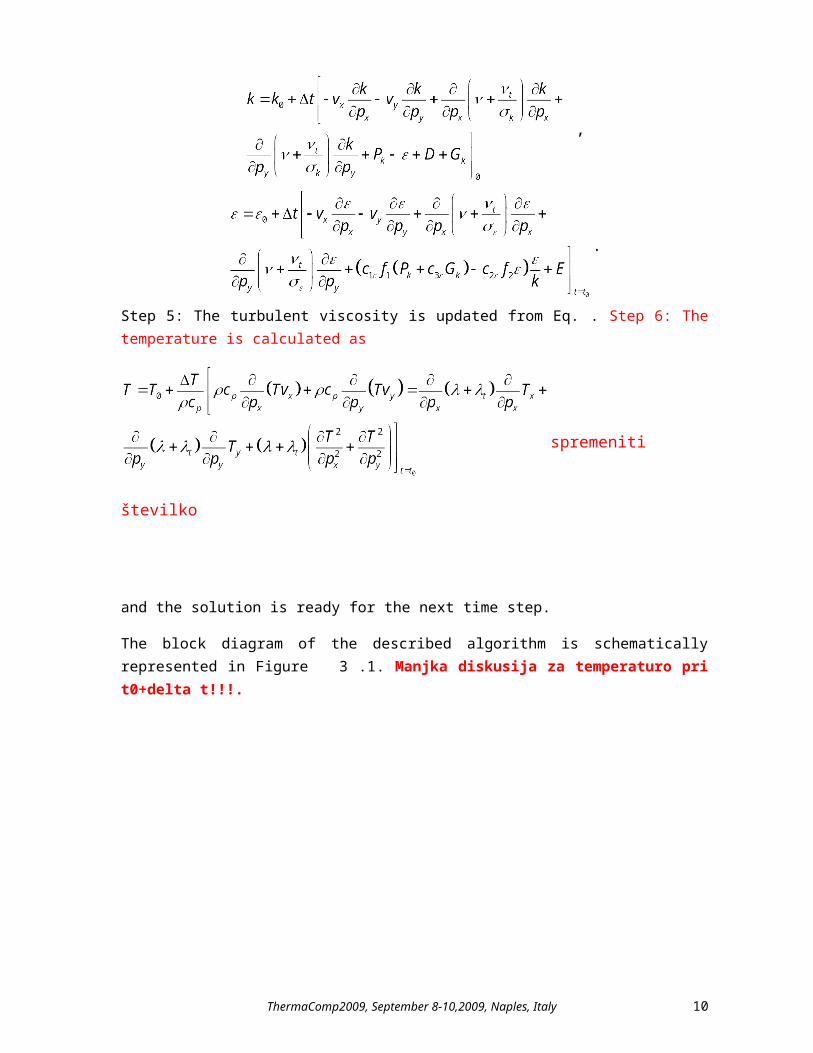
Step 5: The turbulent viscosity is updated from Eq. . Step 6: The temperature is calculated as

spremeniti številko


and the solution is ready for the next time step.

The block diagram of the described algorithm is schematically represented in Figure 3.1. Manjka diskusija za temperaturo pri t0+delta t!!!.

Figure 3.1: Block diagram of the numerical algorithm (manjka temperatura !!!).

3.1 Initial conditions

It is well known that all involved five transport Eqs. (2.1, 2.2, 2.3, 2.4, 2.8, 2.9!!!) , , and are strongly coupled. So it is very important how we choose the initial conditions for each transport variable. The initial conditions for velocity components are obtained by solving the potential field

,

where stands for the velocity potential. Laplace Eq. is solved by the same approach as pressure equation . The following boundary conditions are used

At the inlet boundaries and solid walls, the Neumann boundary conditions for velocity potential are prescribed

.

At the outlet boundaries, the Dirichlet boundary conditions for velocity potential are set to

.


initialization of variables , , , and .

solution of intermediate velocity, Eqs. (3.1) and (3.2)

solution of pressure, Eq. (3.3)

correction of velocity, Eqs. (3.4) and (3.5)

solution of and , Eqs. (3.6) and (3.7)

updating of the turbulent viscosity, Eq. (2.7) and go to step 1

1

2

3

4

5

set calculated values to initial values

After solving the potential flow field, the velocity field in the domain is obtained by the following relations

, .

This procedure guarantees the solenoidality of the initial velocity field. Dodati diskusijo za initial conditions za temperaturo.

In order to prescribe the proper initial conditions for and , two different techniques might be employed:

Use of the uniform profile for both and . A few thousand time steps have to be performed usually with smaller time step to achieve the consistency between the velocity, pressure, turbulent energy and dissipation equation. When the large mismatch of the calculated flow variables with the governing equations at the initial times is reduced, larger time steps can be used.

Use of the assumption of turbulent equilibrium [Yoder and Georgiadis (1999)], where the production of turbulent kinetic energy equals the rate of dissipation. In order to use this technique, another turbulence model, usually algebraic model, is first run to get initial values of the turbulent viscosity.

In this work, the turbulence transport variables are initialized by the first approach.

3.2 Boundary conditions

Three different types of boundaries have to be considered in the present paper: inlet, outlet and wall. The following boundary conditions are used at these boundaries:

At the inlet boundary, the Dirichlet boundary conditions for velocity components, and and temperature are prescribed.

At the outlet boundary, the Neumann boundary conditions for velocity components, and and temperature are prescribed and set to zero.

At the symmetry line, the same Neumann boundary conditions as for the outlet boundary are used, except for the velocity component, perpendicular to the symmetry line, where the Dirichlet boundary conditions are prescribed and set to zero. (ta modri odstavek gre v celoti ven!)

At the wall, the Dirichlet no-slip boundary conditions are set, which implies that the velocity components, as well as and are set to zero. The Dirichlet boundary conditions are set for the hot (left) and cold (right) wall temperature.

The boundary conditions for pressure Eq. at inlet and wall boundaries are of the Neumann type, i.e.

,

where the and are the components of the normal vector in and directions. and

have the following form

(skrajšal za eno enačbo)


where are intermediate velocities, solved by the Eqs. for and at the wall. In Eqs.

and , the represent the wall velocities at . At the outlet boundary, the Dirichlet

boundary conditions for pressure are used and set to zero.

3.3 Radial basis function collocation method

The representation of function over a set of (in general) non-equally spaced nodes

is made in the following way

,

stands for the shape functions, for the coefficients of the shape functions, and represents the number of the shape functions. The left lower index on entries of Eq. represents the domain of influence on which the coefficients are determined. The domains of influence

can in general be contiguous (overlapping) or non-contiguous (non-overlapping). Each of the

domains of influence includes grid-points of which are in the domain and are on the boundary. Typical domains of influence are shown in Figure 3.2.

Figure 3.2: Typical corner, boundary, and interior 5 - noded domains of influence.

The coefficients can be calculated from the nodal values in the domain of influence at least by two distinct ways. The first way is collocation (interpolation) and the second way is approximation by the least squares method. Only the more simple collocation version for calculation of the coefficients is considered in this paper. Let us assume the known function values in the nodes

of the domains of influence . The collocation implies

.


For the coefficients to be computable, the number of the shape functions has to match the number of the collocation points , and the collocation matrix has to be non-singular. The system of Eqs. can be written in a matrix - vector notation

; ; .

The coefficients can be computed by inverting the system (14)

.

By taking into account the expressions for the calculation of the coefficients , the collocation

representation of function on the domain of influence can be expressed as

.

The first partial spatial derivatives of in the domain of influence can be expressed as

; .

The second partial spatial derivatives of in the domain of influence can be expressed as

; .

The radial basis functions, such as multiquadrics, can be used for the shape function

,

where represents the shape parameter and the radial distance between two points in the sub-

domain. The is scaled by the maximum distance between sub-domain points in and directions

,

where is the maximum distance between any of the sub-domain points in the direction .

The shape parameter is fixed for all sub-domains, and set to 32 [2] in all numerical examples of the present paper. The accuracy of the results increases with increased value of the shape parameter, however the condition number of the collocation matrix worsens. The chosen value 32 represents a reasonable balance between both trends. All sub - domains are chosen to contain five nodes as depicted in Figure 3.2.


4 NUMERICAL EXAMPLE

The geometry of the problem is a vertical channel of width and height , ., see Figure 4.3. The flow with constant uniform velocity and temperature is entering into the channel at the bottom and leaving the channel at the top. Vertical walls are kept at different (left wall hot, right wall cold), but constant temperatures. At the outlet, the flow is assumed to be fully developed. The forced flow and the buoyancy force drive the flow upward near the hot wall (adding flow at the left wall), and downward near the cold wall (opposing flow at the right wall). The Reynolds number based on the channel width is set to 4494, and the Grashof number based on the temperature difference between the vertical walls and the channel width is 9.6×105.

Figure 4.3: Schematic of the problem.

Calculations were performed on a node arrangement with 81x171 nodes (without 4 corner nodes), which was found sufficiently fine to obtain a reasonably grid-independent solution. Tu je potrebno povedati kakšna diskretizacija je bila še poskušana in kakšna je razlika med njo in uporabljeno diskretizacijo. The discretization in vertical direction is uniform and in the horizontal

direction is non-uniform, sufficiently refined near the walls to achieve the position of the first point to be in the range at each of the vertical walls, see Figure 4.4. Tu je potrebno napisati še formulo, da bodo rezultati ponovljivi. The time step was used.


Figure 4.4: Detail view of the 81x171 node arrangement. Symbols represents: -boundary nodes and -domain nodes. In the vertical direction only each xxx-th vertical row of discretization points is shown.

The results are presented as the dimensionless variables, i.e. , and for velocity,

temperature and the kinetic energy, respectively. They are non-dimensionalised with the variables on each wall by the following relations

,

,

,

with , and standing for the friction velocity, wall temperature and the friction

temperature, respectively. The friction velocity is defined as

,

with standing for the wall shear stress. Friction temperature is calculated by the following expression

,


where is the heat flux at the wall.

Figure 4.5 and Figure 4.6 are representing the non-dimensional velocity profile of the aiding and opposing flow at the outlet. The prediction of the velocity profile in the region near the walls (viscous sub - layer) agrees very well with the DNS data. In the outer layer, the LS model over-predicts the DNS data, which is a normal behaviour of the LS model [Wilcox, 1993; Bredberg, 2001; Billard et al., 2008, urediti citiranje s številkami!!!]. A better agreement with the DNS data is obtained by the AKN model, which predicts the velocity profile very well in both regions.

The non - dimensional turbulent kinetic energy is represented in Figure 4.7 and Figure 4.8 for the aiding and opposing flow, respectively. On the aiding flow side, the kinetic energy is under-predicted, also out of the viscous sub-layer region. The reason could be in anisotropy of the Reynolds stresses, which was found by the DNS solution to be enhanced in the aiding flow. However, is seems that the anisotropy does not affect the prediction of the velocity field, especially when the AKN model is used, see Figure 4.5, Figure 4.6 and Figure 4.11. The kinetic energy of the opposing flow agrees very well, since it was reported by the DNS data, that the anisotropy of the Reynolds stresses in this region is weakened.

The temperature profile is shown in Figure 4.9 and Figure 4.10 for the hot (aiding flow) and cold (opposing flow) walls, respectively. For the opposing flow, the calculated results are in good agreement with the DNS. However, on the aiding side, we observe larger differences between the low - Re models and DNS. The reason could be in modeling the turbulent diffusivity and turbulent viscosity with a constant turbulent Prandtl number (set to 0.9 in this work). This assumption holds only for simple boundary layer flows, where the velocity and the temperature fields develop simultaneously [10]. In our case, the similarity between the temperature and velocity fields does not hold, since the boundary layer is affected by the buoyancy force. It was observed from the DNS [9] and LES [18] results, that the buoyancy force effects the velocity fluctuations differently as the temperature fluctuations. The velocity fluctuations are enhanced in the opposing flow and reduced in the aiding flow, while the opposite effects are observed for the temperature fluctuations. For better prediction of such behaviours, the turbulent diffusivity should be modelled by the two-equation models for thermal field [10, 14].

Due to the buoyancy effects, the velocity and temperature profiles at the outlet become un-symmetric. This behaviour is shown in Figure 4.11 and Figure 4.12 for the velocity and temperature, respectively. The results are presented by the following non - dimensional relations

,

,

where is standing for the normalized mean temperature. is friction velocity, calculated from

the wall shear stress, averaged on the two walls, i.e. cold and hot walls. stands for friction temperature, calculated by the following equation

,


where is calculated from the averaged wall heat flux, i.e.

.

The Eq. is used for calculating the and on the hot and cold walls, respectively. We can

conclude, that the AKN model predicts the velocity profile with a very good accuracy, while the LS model over - predicts the velocity profile. The temperature profile is over-predicted by both models for the aiding flow, and agrees very good with the DNS data for the opposing wall.

Figure 4.5: Dimensionless velocity profile of the aiding flow in wall coordinates. -DNS solution [8], dashed line-represents LRBFCM with LS model, dash-dot-dashed line-represents LRBFCM with AKN model.


Figure 4.6: Dimensionless velocity profile of the opposing flow in wall coordinates. -DNS solution [8], dashed line-represents LRBFCM with LS model, dash-dot-dashed line-represents LRBFCM with AKN model.

Figure 4.7: Dimensionless kinetic energy of the aiding flow in wall coordinates. -DNS solution [8], dashed line represents LRBFCM with LS model, dash-dot-dashed line represents LRBFCM with AKN model.


Figure 4.8: Dimensionless kinetic energy of the opposing flow in wall coordinates. -DNS solution [8], dashed line represents LRBFCM with LS model, dash-dot-dashed line represents LRBFCM with AKN model.

Figure 4.9: Dimensionless temperature profile of the aiding flow in wall coordinates. -DNS solution [8], dashed line-represents LRBFCM with LS model, dash-dot-dashed line represents LRBFCM with AKN model.


Figure 4.10: Dimensionless temperature profile of the opposing flow in wall coordinates. -DNS solution [8], dashed line represents LRBFCM with LS model, dash-dot-dashed line represents LRBFCM with AKN model.

Figure 4.11: Dimensionless velocity profile at the outlet in wall coordinates. -DNS solution [8], dashed line represents LRBFCM with LS model, dash-dot-dashed line represents LRBFCM with AKN model.


Figure 4.12: Dimensionless temperature profile at the outlet in wall coordinates. -DNS solution [8], dashed line represents LRBFCM with LS model, dash-dot-dashed line represents LRBFCM with AKN model.

The accuracy of the represented method was also evaluated as a function of Nusselt number and skin friction at the top of the channel (at the outlet), which are calculated by the following equations

,

,

respectively. In Eqs. and , is a bulk-averaged quantity over , which is the interval from the wall to the maximum velocity location. The results are presented in Table 4.3, where excellent agreement was achieved with both turbulence models used.

Table 4.3: Nusselt number and skin friction at the channel outlet.

turbulencemodel

aiding flow opposing flow

[Kasagi and Nishimura, 1997],

DNS/ 7.42 9.9E-3 20.94 7.9E-3

present method LS 6.67 9.96E-3 23.18 7.30E-3AKN 7.96 1.05E-2 23.91 7.87E-3

5 CONCLUSIONS

This paper probably for the first time represents a solution of the incompressible turbulent thermo fluid problem by a meshless method. The low-Re models with the two types of closure coefficients, proposed by LS [ref] and AKN [ref] are used. The novel numerical solution is based on


the local collocation with the radial basis functions for spatial disretization and the first order (backward Euler) explicit method for the time discretization. Due to its locality and explicit time stepping, the method appears very suitable for parallelization. The partial differential equations are solved in their strong form and no integrations are involved. The transition from two - dimensional to three - dimensional cases is from the coding point of view quite straightforward. The results were compared with the DNS for a problem of combined forced and natural convection with a reasonably good agreement, with both LS and AKN turbulence models. However, better prediction of the velocity field was obtained by the AKN model. The prediction of the temperature field was obtained with a slightly less accuracy as the velocity field. The reason is not in the present novel numerical method, but in using the simplified model for the turbulent diffusion. In the future, the method will be extended to cope with the turbulent flows with solidification, as encountered for example in the continuous casting of steel. With this, the LRBFCM will additionally strengthen its already established reputation as a simple, accurate, robust, and reliable novel meshless computational method.

Acknowledgement: The authors would like to express their gratitude to Slovenian Technology Agency (RV) and Slovenian Research Agency (BŠ) for funding of the represented research. This paper represents an extended version of the paper presented at the First International Conference on Computational Methods in Thermal Problems, September 8 - 10, 2009 in Naples, Italy. The authors wish to acknowledge the organisers for invitation to publish the paper in the present Journal.

REFERENCES

[1] B. Šarler, From Global to Local Radial Basis Function Collocation Method for Transport Phenomena, in: V.M.A. Leitao, C.J.S. Alves, C. Armando-Duarte, Advances in Meshfree Techniques, (Computational Methods in Applied Sciences, Vol.5), Springer Verlag, Dordrecht , 257 - 282, 2007.

[2] B. Šarler and R. Vertnik, Meshfree local radial basis function collocation method for diffusion problems, Computers and Mathematics with Application, 51, 1269 - 1282, 2006.

[3] R. Vertnik and B. Šarler, Meshless local radial basis function collocation method for convective diffusive solid-liquid phase change problems, International Journal of Numerical Methods in Heat and Fluid Flow, 16, 617 - 640, 2006.

[4] R.Vertnik and B.Šarler, Solution of Incompressible Turbulent Flow by a Mesh-Free Method, Computer Modeling in Engineering & Sciences, 44, 66 - 95, 2009.

[5] G. Kosec and B.Šarler, Solution of heat transfer and fluid flow problems by the simplified explicit local radial basis function collocation method, International Journal of Numerical Methods for Heat & Fluid Flow, 18, pp. 868 - 882, 2008.

[6] B. E. Launder and B. I. Sharma, Application of the energy-dissipation model of turbulence to the calculation of flow near a spinning disc. Letters in Heat and Mass Transfer, 1, 131 - 138, 1974.

[7] A. J. Chorin, A numerical method for solving incompressible viscous flow problems, Journal of Computational Physics, 2, 12 - 26, 1967.

[8] Y. T. Gu, G. R. Liu, G. R. Meshless technique for convection dominated problems. Computational Mechanics, 38, 171 - 182, 2005.

[9] N. Kasagi, and M. Nishimura, Direct numerical simulation of combined forced and natural turbulent convection in a vertical plane channel, International Journal for Heat and Fluid Flow, 18, 88 - 99, 1997.


[10] K. Abe, T. Kondoh and Y. Nagano, A new turbulence model for predicting fluid flow and heat transfer in separating and reattaching flows-II. Thermal field calculations. International Journal of Heat and Mass Transfer, 38, 1467 - 1481, 1995.

[11] D. C. Wilcox, Turbulence modeling for CFD, DCW Industries, Inc., California, 1993.

[12] J. Bredberg, On two-equation Eddy-Viscosity Models. Internal Report 01/8, Department of Thermo and Fluid Dynamics, Chalmers University of Technology, Göteborg, Sweden.

[13] Y. T. Chen, J. H. Nie, B. F. Armaly, H. T. Hsieh, Turbulent separated convection flow adjacent to backward-facing step - effects of step height, International Journal of Heat and Mass Transfer, 49, 3670 - 3680, 2006.

[14] F. Billard, J. C. Uribe, D. Laurence, A new formulation of the - model using elliptic blending and its application to heat transfer prediction, Proceedings of 7th International Symposium on Engineering Turbulence Modelling and Measurements, Editors: M.A. Leschziner, 89-94, Limassol, Cyprus, June 4 - 6, 2008.

[15] T. Yilmaz, S. M. Fraser, Turbulent natural convection in a vertical parallel-plate channel with asymmetric heating, International Journal of Heat and Mass Transfer, 50, 2612 - 2623, 2007.

[16] A. Keshmiri, Y. Addad, M. A. Cotton, D. R. Laurence, F. Billard, Refined eddy viscosity schemes and large eddy simulations for ascending mixed convection flows, Proceedings of CHT-08 ICHMT International Symposium on Advances in Computational Heat Transfer, CHT-08-407, Marrakesh, Morocco, May 11 - 16, 2008.

[17] J. Yin, D. J. Bergstrom, LES of combined forced and natural turbulent convection in a vertical slot. Computational Fluid Dynamics 2004, Springer Berlin Heidelberg, 567 - 572, 2006.

[18] B. C. Wang, E. Yee, J. Yin, D. J. Bergstrom, A general dynamic linear tensor-diffusivity subgrid-scale heat flux model for large-eddy simulation of turbulent thermal flows. Numerical Heat Transfer, 51B, 205-227, 2007.

[19] E. Divo, A. J. Kassab, An efficient localized RBF meshless method for fluid flow and conjugate heat transfer. ASME Journal of Heat Transfer, 129, 124 - 136, 2007.

[20] C. K. Lee, X. Liu, S. C. Fan, Local multiquadric approximation for solving boundary value problems. Computational Mechanics, 30, 396 - 409, 2003.

[21] R. A. W. M. Henkes, F. F. van der Vlugt and C. J. Hoogendoorn, Natural-convection flow in a square cavity calculated with low-Reynolds-number turbulence models. International Journal of Heat and Mass Transfer, 34(2), 377 - 388, 1991.

[22] K. J. Hsieh, F. S. Lien, Numerical modelling of buoyancy-driven turbulent flows in enclosures. International Journal of Heat and Fluid Flow, 25, 659 - 670, 2004.

[23] Y. Zhou, R. Zhang, I. Staroselsky, H. Chen, Numerical simulation of laminar and turbulent buoyancy-driven flows using a lattice Boltzmann based algorithm. International Journal of Heat and Mass Transfer, 47, 4869 - 4879, 2004.

[24] F. Ampofo, T. G. Karayiannis, Experimental benchmark data for turbulent natural convection in an air filled square cavity. International Journal of Heat and Mass Transfer, 46, 3551 - 3572, 2003.

[25] H. Le, P. Moin, J. Kim, Direct numerical simulation of turbulent flow over a backward-facing step. Journal of Fluid Mechanics, 330, 349 - 374, 1997.

[26] H. Lin, S.N. Atluri, S.N.Meshless local Petrov-Galerkin (MLPG) method for convection diffusion CMES: Computer Modeling in Engineering & Sciences, 1, 45 - 60, 2000.

[27] S.N. Atluri, S. Shen, The Meshless Method, Tech Science Press, Encino, 2002.


[28] P. Breitkopf, A. Huerta (Eds.), Meshfree and Particle Based Approaches in Computational Mechanics, Kogan Page Science, London, 2003.

[29] S.N. Atluri, The Meshless Method (MLPG) for Domain and BIE Discretization, Tech Science Press, Forsyth, 2004.

[30] G.R. Liu, Y.T. Gu, An Introduction to Meshfree Methods and Their Programming, Springer, Dordrecht, 2005.

[31] S. Li, W.K. Liu, Meshfree Particle Methods 2nd Corrected Printing, Springer Verlag, Berlin, 2007.

[32] G.R. Liu, Mesh Free Methods, Second Edition, CRC Press, Boca Raton, 2009.

[33] G. E. Fasshauer, Meshfree Approximation Methods with MATLAB, Interdisciplinary Mathematical Sciences, Vol. 6, World Scientific Publishers, Singapore, 2007.

[34] A.J.M. Ferreira, E.J. Kansa, G.E. Fasshauer, VMA. Leitãao (Eds.), Progress on Meshless Methods, Computational Methods in Applied Sciences, Vol. 11, Springer, Berlin, 2009.

[35] S.N. Atluri, B. Šarler (Eds.), Proceedings of the 5th ICCES Symposium on Meshless Methods, University of Nova Gorica Press, Nova Gorica, 2009.

[36] M.D. Buhmann, Radial Basis Functions, Cambridge University Press, Cambridge, 2000.

[37] E.J. Kansa, Multiquadrics - a scattered data approximation scheme with application to computational fluid dynamics, I - surface approximations and partial derivative estimates, Computers and Mathematics with Applications, vol. 19, pp. 127-145, 1990.

[38] E.J. Kansa, Multiquadrics - a scattered data approximation scheme with application to computational fluid dynamics, II – solutions to parabolic, hyperbolic and elliptic partial differential equations, Computers and Mathematics with Applications, vol. 19, pp. 147-161, 1990.


http://www.worldscibooks.com/mathematics/6437.html

abstract title - ung.sisabotin.ung.si/~sarler/vertnik/aamm_paper_rv_bs_03.01... · web viewthey...

Documents