Technical Report 131

Accommodating a Flexible Response Heterogeneity Distribution in Choice Models of Human Behavior for Transportation Planning Chandra Bhat Center for Transportation Research February 2018

Data-Supported Transportation Operations & Planning Center (D-STOP)

A Tier 1 USDOT University Transportation Center at The University of Texas at Austin

D-STOP is a collaborative initiative by researchers at the Center for Transportation Research and the Wireless Networking and Communications Group at The University of Texas at Austin.

DISCLAIMER The contents of this report reflect the views of the authors, who are responsible for the facts and the accuracy of the information presented herein. This document is disseminated under the sponsorship of the U.S. Department of Transportation’s University Transportation Centers Program, in the interest of information exchange. The U.S. Government assumes no liability for the contents or use thereof.

Technical Report Documentation Page

1. Report No.

D-STOP/2017/131 2. Government Accession No.

3. Recipient's Catalog No.

4. Title and Subtitle

Accommodating a Flexible Response Heterogeneity Distribution in

Choice Models of Human Behavior for Transportation Planning

5. Report Date

February 2018 6. Performing Organization Code

7. Author(s)

Chandra R. Bhat and Patricia S. Lavieri

8. Performing Organization Report No.

Report 131

9. Performing Organization Name and Address

Data-Supported Transportation Operations & Planning Center (D-

STOP)

The University of Texas at Austin

3925 W. Braker Lane, Stop D9300

Austin, Texas 78759

10. Work Unit No. (TRAIS)

11. Contract or Grant No.

DTRT13-G-UTC58

12. Sponsoring Agency Name and Address

Data-Supported Transportation Operations & Planning Center (D-

STOP)

The University of Texas at Austin

3925 W. Braker Lane, Stop D9300

Austin, Texas 78759

13. Type of Report and Period Covered

14. Sponsoring Agency Code

15. Supplementary Notes

Supported by a grant from the U.S. Department of Transportation, University Transportation Centers

Program. 16. Abstract

In this report, we propose a general copula approach to accommodate non-normal continuous mixing

distributions in multinomial probit (MNP) models. In particular, we specify a multivariate mixing

distribution that allows different marginal continuous parametric distributions for different coefficients. A

new hybrid estimation technique is proposed to estimate the model, which combines the advantageous

features of each of the maximum simulated likelihood inference technique and Bhat’s maximum

approximate composite marginal likelihood (MACML) inference approach. The effectiveness of our

formulation and inference approach is demonstrated through simulation exercises and an empirical

application.

17. Key Words

Copula, heterogeneity, MACML,

multinomial probit, choice modeling

18. Distribution Statement

No restrictions. This document is available to the public

through NTIS (http://www.ntis.gov):

National Technical Information Service

5285 Port Royal Road

Springfield, Virginia 22161 19. Security Classif.(of this report)

Unclassified 20. Security Classif.(of this page)

Unclassified 21. No. of Pages

42 22. Price

Form DOT F 1700.7 (8-72) Reproduction of completed page authorized

iv

Disclaimer

The contents of this report reflect the views of the authors, who are responsible for the

facts and the accuracy of the information presented herein. This document is

disseminated under the sponsorship of the U.S. Department of Transportation’s

University Transportation Centers Program, in the interest of information exchange. The

U.S. Government assumes no liability for the contents or use thereof.

The contents of this report reflect the views of the authors, who are responsible for the

facts and the accuracy of the information presented herein. Mention of trade names or

commercial products does not constitute endorsement or recommendation for use.

Acknowledgements

This research was partially supported by the U.S. Department of Transportation through

the Data-Supported Transportation Operations and Planning (D-STOP) Tier 1 University

Transportation Center. The first author would like to acknowledge support from a

Humboldt Research Award from the Alexander von Humboldt Foundation, Germany.

This report under the title of “A New Mixed MNP Model Accommodating a Variety of

Dependent Non-Normal Coefficient Distributions” by C.R. Bhat and P.S. Lavieri was

published in Theory and Decision, 84(2), 239-275, 2018.

.

v

TABLE OF CONTENTS

Chapter 1. Introduction ......................................................................................................1

Chapter 2. Copula Basics ...................................................................................................5

2.1 The Gaussian Copula ....................................................................................................6

Chapter 3. The Model .........................................................................................................8

3.1 Model Estimation Using the Hybrid MSL-MACML Approach ..................................9

3.2 Alternative Estimation Procedure ..............................................................................16

Chapter 4. Simulation Evaluation ...................................................................................18

4.1 Performance Evaluation .............................................................................................21

4.2 Simulation Results ......................................................................................................21

Chapter 5. An Empirical Application .............................................................................24

5.1 Valuation of Travel Time Savings .............................................................................24

5.2 Empirical Results .......................................................................................................25

5.2.1 Data Fit and VTTS Estimates .......................................................................26

5.2.2 Estimation Results for the Preferred Model (Model 12) ..............................30

Chapter 6. Summary and Conclusions ...........................................................................32

1

Chapter 1. Introduction

Econometric discrete choice analysis constitutes the underlying framework for analyzing

demand for a variety of consumer commodities and services. For many decades, the discrete

choice model employed was the multinomial logit (MNL) model (Luce and Suppes, 1965 and

McFadden, 1974), which assumes a single composite independently and identically distributed or

IID (across alternatives) random utility error term with a Gumbel (or Type I extreme-value)

distribution. However, over the past two decades, it has become much more common place to

acknowledge the presence of unobserved taste sensitivity in response to variables, as well as

accommodate non-IID kernel error terms across alternatives. A general approach to do so is to

use a multivariate normal kernel mixed with an appropriately distributed random coefficients

vector, which we will label as the mixed multinomial probit (or mixed MNP) model.1

An important consideration in the random multivariate mixing (random coefficients)

distribution is to explicitly specify it in a way that is consistent with theoretical notions. In fact,

the ability to do so is critical to the observation made by McFadden and Train (2000) that the

mixed model (whether with an extreme value kernel or an MNP kernel) is capable of

approximating any random utility maximization model.2 For example, it is possible that an

analyst may want to specify a naturally bounded distribution (such as a log-normal distribution

or a Rayleigh distribution) for cost and time coefficients in a travel choice model, so that the

coefficients are strictly negative. Indeed, several studies (see, for example, Amador et al., 2005,

Train and Sonnier, 2005, Hensher et al., 2005, Balcombe et al., 2009, and Torres et al., 2011)

have underscored the potentially serious misspecification consequences (in terms of theoretical

considerations, data fit, as well as trade-off evaluations) of using an unbounded distribution

(specifically the normal distribution). Besides, another issue with using an unbounded

distribution that straddles the zero value for the cost coefficient is that it leads to a breakdown of

the willingness to pay (WTP) calculations (see Cedilnik et al., 2006, Daly et al., 2011).

Bhat and Sidharthan (2012) developed a mixed MNP model using a multivariate skew-

normal (MVSN) mixing distribution (see also Bhat et al., 2015). This model is very effective

because the mixing of the MVSN random coefficients distribution with an independent MVN

kernel distribution puts the composite error term back to an MVSN form. The MVSN

distribution retains several attractive properties of the multivariate normal distribution. It is

tractable, parsimonious in parameters that regulate the distribution and its skewness, and includes

the multivariate normal distribution as a special interior point case. It also is a very flexible

1An analogous structure may be obtained by essentially adding an IID Gumbel error term across alternatives to the

multivariate normal coefficients, leading to a mixed multinomial logit model; see Bhat, 1997 and Revelt and Train,

1998 for the first multivariate applications of this type of a model. Alternatively, one can add a multivariate extreme

value (MEV) error vector kernel to the utility of the alternatives, combined with additional non-identical kernel error

terms, to the random coefficients vector (see, for example, Bhat and Guo, 2007). But, as discussed in detail in Bhat

(2011), all these structures essentially achieve the same purpose, and the choice is simply a matter of convenience.

Besides, the use of an MNP kernel has substantial advantages when combined with recently proposed analytic

methods of evaluating a multivariate cumulative normal distribution (MVNCD) function that have been shown to be

much more computationally efficient than traditional simulation approaches. Also, when extensions to accommodate

correlation across decision makers due to spatial and/or social interactions are considered, the MNP kernel is much

easier and more efficient. We will henceforth focus in this report on the MNP kernel. 2 Just to clarify a myth. The mixed multinomial logit model is no more general than the mixed MNP model, as long

as we allow the mixing distribution with the MNP kernel to be non-normal, as we do so in the current report.

2

unimodal density structure that can replicate a variety of smooth unimodal density shapes with

tails to the left or right as well as with a high modal value (sharp peaking) or low modal value

(flat plateau). The skewness to the right or left is generated by moving probability mass to the

left or right of the mean of the normal distribution but keeping the tails thin as in the normal

density function, which helps substantially in estimation. In particular, a left-skew is generated

by keeping the left tail similar to that of the normal density function, but very sharply reducing

the tail on the right side of the mode (see Capitanio, 2010 for a discussion of the rate of decrease

in the tail distributions of the skew-normal density function). Thus, to employ a cost coefficient

that is strictly constrained to the negative domain, all that the analyst needs to do is to pre-impose

a very high skew parameter with a location parameter that is negative (essentially, with a very

high skew parameter imposed, the probability density function drops to zero at the location

parameter without any overlap on zero; that is, a skew-normal collapses to the so-called half-

normal density function with no density to the right of the negative location parameter; see

Azzalini, 2013). Additionally, the MVSN-mixed MNP lends itself nicely to estimation using

Bhat’s (2011) maximum approximate composite marginal likelihood (MACML) approach.

In this report, we propose an even more general copula-based approach to accommodate

non-normal continuous mixing distributions than that proposed in Bhat and Sidharthan (2012).3

Specifically, the copula-based mixed random coefficients MNP model proposed in this report

allows a multivariate mixing distribution that can combine any continuous distributional shape

for each coefficient, including (but not limited to) the skew-normal distribution. This extends the

type of continuous multivariate distributions one may want to test, with the only restriction being

that the individual coefficient distributions should be continuous. The procedure is based on

generating a multivariate continuous distribution through the use of specified parametric

univariate continuous coefficient distributions (that can be different for different coefficients)

combined with a Gaussian Copula, and is based on Sklar’s theorem (Sklar, 1959; see also Bhat

and Eluru, 2009 and Joe, 2015). While one may use other copulas to join the different univariate

distributions to generate a multivariate distribution, the Gaussian copula used here has many

advantages. For instance, the Gaussian copula includes the case of independence across specific

coefficients, allows a very flexible and wide range of dependence across coefficients, and is

relatively easy to simulate relative to other copula types. It allows dependence across the random

coefficients, even if the random coefficients take different marginal distributions. Most

importantly, it is the best copula to work with in situations where the analyst is prepared to

accept a normal density function for many coefficients, with relatively fewer coefficients

specified to have non-normal parametric univariate density functions. This is because, as we will

note later, the Gaussian copula requires an integral transformation of each marginal variate into a

normal marginal variate. When there are many normal marginal variates, this transformation is

3 Discrete distributions may also be used for the mixing. If the mixing vector is assumed to take M possible value

states with state-specific probabilities, this leads to the familiar latent class model used in marketing (see Kamakura

and Russell, 1989) and transportation (see Bhat, 1997). On the other hand, if a discrete distribution is considered

separately for each individual random coefficient, this is essentially a non-parametric random coefficients model

(see Bastin et al., 2010, Berry and Haile, 2014, il Kim, 2014). The non-parametric specification allows consistent

estimates of the observed variable effects under broad model contexts by making regularity (for instance,

differentiability) assumptions on an otherwise distribution-free density form. But the flexibility of these methods

comes at a high inferential cost since consistency is achieved only in very large samples, parameter estimates have

high variance, and the computational complexity/effort can be substantial (Mittelhammer and Judge, 2011). Overall,

the continuous distribution specification dominates the literature, at least in part because it offers efficiency in the

number of mixing distribution parameters to be estimated.

3

not needed for these variates, so that these variates enter directly in the copula (see Equation (7)

later), which simplifies the copula construction (with associated optimization convergence and

computational speed benefits during model estimation).

The estimation of the copula model is achieved using a combination of the maximum

simulated likelihood (MSL) technique (to accommodate the non-normal random coefficients)

and Bhat’s MACML inference approach (to accommodate all the normal random coefficients as

well as the kernel normal error structure; see Bhat, 2011 and Bhat, 2014). This is the first time

that a hybrid of these two inference approaches has been proposed in the literature. The

combination harnesses the advantages of each of these approaches. The MSL approach is very

general and can be used to estimate models with any distribution for the random coefficients,

including the copula-based model proposed in this report. However, the approach can be

computationally very expensive to ensure good asymptotic estimator properties, and can be

prohibitive and literally infeasible (in the context of the computation resources available and the

time available for estimation) as the number of random coefficients increases. This is because of

the rapid increase in simulation noise and degradation in the accuracy of simulation techniques at

medium-to-high dimensions, leading also to convergence problems during estimation and

difficulty in estimating the covariance matrix of the MSL estimator (see Bhat, 2011). On the

other hand, the MACML approach is simple, computationally very efficient, and simulation-free.

It easily and accurately is able to accommodate even a high number of multivariate normally

distributed random coefficients, providing both more accuracy (smaller bias in parameters) and

orders of magnitude of computational efficiency relative to the MSL inference approach (see

Bhat et al., 2010, Bhat and Sidharthan, 2012, and Paleti and Bhat, 2013). The other advantage is

that the smooth analytically-approximated likelihood function all but ensures convergence during

maximization, and also lends itself nicely to relatively smooth second derivative functions to

compute the covariance matrix of the estimator. However, the MACML estimator is restricted to

normally distributed coefficients or skew-normally distributed coefficients, and does not allow

more general parametric random distributions as in the proposed copula MNP model. The

combination of the MSL and MACML, however, is especially well suited for the case when

there are relatively few non-normally distributed coefficients (so that the simulation does not

involve very high dimensions) and many normally distributed coefficients (so that the MACML

computational accuracy and efficiency can be realized). However, even in the case when many

or even all coefficients are non-normally distributed (with potentially different univariate non-

normal distributions for each coefficient), our proposed copula approach provides a systematic

parametric framework to engender dependencies (due to unobserved factors) across the non-

normal coefficients (rather than pre-imposing independence assumptions on these non-normally

distributed coefficients). Of course, if all the coefficients are assumed non-normal and

independent, our copula-based hybrid approach collapses exactly to an MSL estimation approach

where the univariate integral transforms essentially become vehicles for generating realizations

from each of the non-normal univariate distributions. On the other hand, if all the coefficients are

assumed to follow a multivariate normal distribution, our copula-based hybrid approach

collapses exactly to the MACML estimation approach.

To summarize, in this report, we develop a general copula-based mixed random

coefficients MNP model and propose a hybrid MSL-MACML inference approach for estimation.

We demonstrate the effectiveness of our inference approach through simulation exercises as well

as an empirical application. The rest of this report is structured as follows. The next chapter

presents the basics of copula-based multivariate distributions, with an emphasis on the Gaussian

4

copula. The third chapter presents the proposed model formulation and estimation procedure.

Chapter 4 undertakes simulation exercises to assess the ability of the proposed estimation

procedure to recover underlying parameters. Chapter 5 presents an empirical application of the

model on repeated choices data. Finally, Chapter 6 summarizes the report and identifies future

extensions.

5

Chapter 2. Copula Basics

In this chapter, we provide an overview of copula functions, with an emphasis on the

Gaussian copula. We also use this chapter as preparation for the model formulation in the

subsequent chapter. Readers interested in learning more about copula functions are referred to

Trivedi and Zimmer (2007), Bhat and Eluru (2009), and Joe (2015).

The word copula, as originally coined by Sklar, 1959, originates from the Latin word

“copulare”, which means to tie, bond, or connect. The basic idea here is that a joint distribution

can always be factored into marginal distributions tied together by a dependence function called

the copula. Alternatively, a joint multivariate stochastic dependence relationship (i.e., a

multivariate distribution) can be generated by wrapping pre-specified marginal distributions

together using an appropriately specified dependence structure called the copula. In essence, the

copula approach separates the marginal distributions from the dependence structure, so that the

dependence structure is unaffected by the marginal distributions assumed. This provides

substantial flexibility in correlating random variables, which may not even have the same

marginal distributions. The copulas themselves are multivariate distribution functions defined

over the unit cube linking uniformly distributed marginal distributions, the point being that any

prespecified marginal distribution can be translated into an equivalent uniform distribution using

the integral transform result. So, let C be a K-dimensional copula of uniformly distributed

random variables U1, U2, U3, …, UK with support contained in [0,1]K. Then,

)...,,,Pr(),...,,( 221121 KKK uUuUuUuuuC θ , (1)

where θ is a parameter vector of the copula commonly referred to as the dependence parameter

vector. Now, consider K random variables Y1, Y2, Y3, …, YK, each with univariate continuous

marginal distribution functions )Pr()( kkkk yYyF , k =1, 2, 3, …, K. Then, by the integral

transform result, and using the notation (.)1

kF for the inverse univariate cumulative distribution

function, we can write the following expression for each k (k = 1, 2, 3, …, K):

)).(Pr())(Pr()Pr()( 1

kkkkkkkkkk yFUyUFyYyF (2)

A joint K-dimensional distribution function of the random variables with the continuous

marginal distribution functions )( kk yF can then be generated, using Sklar’s (1973) theorem, as

follows:

).( where),,...,,(

))(),...,(),(Pr(

),...,,Pr(),...,,(

21

222111

221121

kkkK

KKK

KKK

yFuuuuC

yFUyFUyFU

yYyYyYyyyH

θ

(3)

To better understand the generated dependence structures between the original random

variables KYYY ,...,, 21 (that is, between the elements of the Y vector, where ),...,,( 21 KYYYY ),

concordance measures are used. Basically, two random variables are labeled as being concordant

(discordant) if large values of one variable are associated with large (small) values of the other,

and small values of one variable are associated with small (large) values of the other. One of the

most popular concordance measures of dependence in the copula literature is the Spearman’s

6

,S which measures the dependence between any two random variables ),( kj YY as follows. Let

)~

,~

( kj YY and ),( kj YY

be independent copies of ),( kj YY . That is, ),( kj YY , )~

,~

( kj YY , and ),( kj YY

are all independent vector pairings, each with a common bivariate distribution function (.,.)ijF

and univariate margins iF and jF . Then, Spearman’s S is three times the probability of

concordance minus the probability of discordance for the two vectors ),( kj YY and ),~

( kj YY

:

0))(~

(0))(~

(3),( kkjjkkjjkjS YYYYPYYYYPYY

. (4)

The coefficient “3” is a normalization constant, since the expression in parenthesis is bounded in

the region [–1/3, 1/3] (see Nelsen, 2006, pg. 161). It can be shown (see Bhat and Eluru, 2009;

Joe, 2015) that the Spearman S dependence measure for a pair of continuous variables ),( kj YY

is equivalent to the familiar Pearson’s correlation coefficient for the grades of 1Y and 2Y ,

where the grade of jY is )( jj YF and the grade of 2Y is )( kk YF .

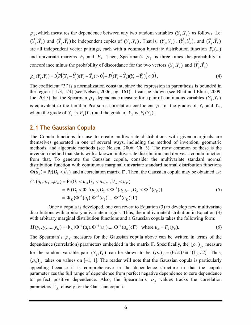
2.1 The Gaussian Copula

The Copula functions for use to create multivariate distributions with given marginals are

themselves generated in one of several ways, including the method of inversion, geometric

methods, and algebraic methods (see Nelsen, 2006; Ch. 3). The most common of these is the

inversion method that starts with a known multivariate distribution, and derives a copula function

from that. To generate the Gaussian copula, consider the multivariate standard normal

distribution function with continuous marginal univariate standard normal distribution functions

)~

Pr()~

( kkk dDd and a correlation matrix Γ . Then, the Gaussian copula may be obtained as:

).);(),...,(),((

))(),...,(),(Pr(

)...,,,Pr(),...,,(

1

2

1

1

1

1

2

1

21

1

1

221121

ΓKK

KK

KKK

uuu

uDuDuD

uUuUuUuuuC

(5)

Once a copula is developed, one can revert to Equation (3) to develop new multivariate

distributions with arbitrary univariate margins. Thus, the multivariate distribution in Equation (3)

with arbitrary marginal distribution functions and a Gaussian copula takes the following form:

).(where),);(),...,(),((),...,,( 1

2

1

1

1

21 kkkKKK yFuuuuyyyH Γ (6)

The Spearman’s S measures for the Gaussian copula above can be written in terms of the

dependence (correlation) parameters embedded in the matrix Γ. Specifically, the jkS )( measure

for the random variable pair ),( kj YY can be shown to be )2/(sin)/6()( 1

jkjkS . Thus,

jkS )( takes on values on [–1, 1]. The reader will note that the Gaussian copula is particularly

appealing because it is comprehensive in the dependence structure in that the copula

parameterizes the full range of dependence from perfect negative dependence to zero dependence

to perfect positive dependence. Also, the Spearman’s S values tracks the correlation

parameters jk closely for the Gaussian copula.

7

Now partition the K-variate random variable vector Y into two sub-vectors Z (of size

E×1) and W )1( L , so that .),( WZY Let the elements of the Z vector each have a pre-

specified but non-normal continuous parametric distribution so that )Pr()( eeee zZzF (note

that the cumulative distribution functions can vary across the elements of Z). Let each element

of the W vector be normally distributed with mean lr and standard deviation l , so that

),()Pr()( *

llll wwWwF where

l

lll

rww

*. Then, defining )( eee zFu , we may write

the multivariate distribution in Equation (6) as:

. )(where,;,...,,,,...,,

,;,...,,),(),...,(),(),...,,,,...,,(

1**

2

*

121

**

2

*

1

1

2

1

1

1

2121

eeLELE

LELELE

ugwwwggg

wwwuuuwwwzzzH

Γ

Γ (7)

The important point to note is that we now have the multivariate distribution of ),( WZY

translated to the multivariate normal distribution of ,),(~

WGY where )]([1

eee ZFG and

.),...,,( 21 EGGGG Next, partition the correlation matrix Γ as follows:

WGW

GWG

ΓΓ

ΓΓΓ . Immediately then, using the conditional distribution properties of the

multivariate normal distribution, and defining ),...,( 21 Lrrrr , ,),...,( 21

Egggg and a

diagonal L×L matrix Ψ with the lth diagonal element being l , we are able to write the

conditional distribution of the vector W conditional on Z as follows:

. )(and

),,(~)()(

ΨΓΓΓΓΨΩΓΨΓ

Ω

11

GWGGWWGGW

LMVN

rgd

dgG|WzZ|W (8)

This conditional distribution for W given Z, while accommodating the dependence between the

two random vectors, plays a central role in the estimation of the proposed Gaussian copula

model, as discussed in the next chapter.

8

Chapter 3. The Model

Consider a repeated choice situation (or a panel situation), with the index q for the

individual, ) ..., ,2 ,1( Qq , index i for the alternative ) ..., ,2 ,1( Ii , and index t for the choice

occasion. For ease in presentation, we will use the same number of choice occasions T for every

individual. Extension to the case of varying number of choice occasions per individual is

straightforward. Also note that the cross-sectional case corresponds to the case of T=1.

Consider the random-coefficients formulation in which the utility that an individual q

associates at time period t with alternative i is written as:

,~~qtiqtiqqtiqqtiU εsγxβ (t=1, 2, 3,…,T) (9)

where qtix is a )1( E -column vector of exogenous attributes (without including constants), qtis

is another )1( L -column vector of exogenous attributes (including dummy variables for

constants, except in one of the I alternative utilities, say the first alternative), qβ is an individual-

specific )1( E -column vector of coefficients that varies across individuals based on unobserved

individual attributes and with each element having a non-normal univariate distribution function

).()Pr( eeeqe zFz qγ is another individual-specific )1( L -column vector of MVN-

distributed coefficients that varies across individuals based on unobserved individual attributes,

with each of its elements having a normal univariate distribution function

.),()Pr( **

l

lllllql

rwwww

Define ),( qqq γβα . The correspondence of our notations

with the previous chapter should now be clear, with qβ taking the place of Z, qγ taking the place

of W, and ),( qqq γβα corresponding to ),( WZY . Then, following the previous chapter,

we may write the joint cumulative multivariate distribution of ),( qqq γβα exactly as in

Equation (7) after translating it into an equivalent joint cumulative multivariate standard normal

distribution of ),~

(~ qqq γβα , with )]([~ 1

qeeqe F and .)~

,...,~

,~

(~

21 qEqqq β The

correlation matrix Γ (of dimension ))()( LELE in Equation (7) is partitioned as

γγβ

γββ

ΓΓ

ΓΓΓ

~

~~

. Following Equation (8) and the definitions just preceding that equation, we

write:

. and

),,(~)~

(|)(|

~~~~~ Ψ)ΓΓΓ(ΓΨΩΓΓΨ

Ωβγβγ

11

γββγβγqβγβq

qLqqqqqqMVN

rgd

dgz (10)

The (I×1)-vector of kernel error terms, )~,,~,~,~(~321

qtIqtqtqtqt εεεε ε , at each choice occasion is

assumed to have a general covariance structure subject to identifiability considerations so that

).,(MVN~~ Θ0εqt (note that the qtε~ error terms are considered independent across individuals

and choice occasions, and qtε~ is assumed independent of ),( qqq γβα ; the random vector qα

is also independent across individuals). Since only utility differences matter in discrete choice

9

models, appropriate identification conditions need to be maintained. While there are many ways

to ensure identification, a common approach is to take the differences of the error terms with

respect to the first error term. Let ),~~( 11 qqiqi εεε and let ),,,( 131211 qIqqq ε...εεε . Then, up to a

scaling factor, the covariance matrix of 1qε )~

say( 1Θ is identifiable. Next, scale the top left

diagonal element of this error-differenced covariance matrix to 1. Thus, there are

1)]2/()1[( II free covariance terms in the )1()1( II matrix 1

~Θ . Θ is constructed

from 1

~Θ by adding a top row of zeros and a first column of zeros.

In addition to the identification condition just discussed, in the case of cross-sectional

data, the elements of qγ corresponding to the dummy variables for alternative-specific constants

will need to be fixed, and will not have a random distribution. This is because the kernel error

terms already absorb the randomness in the constants.

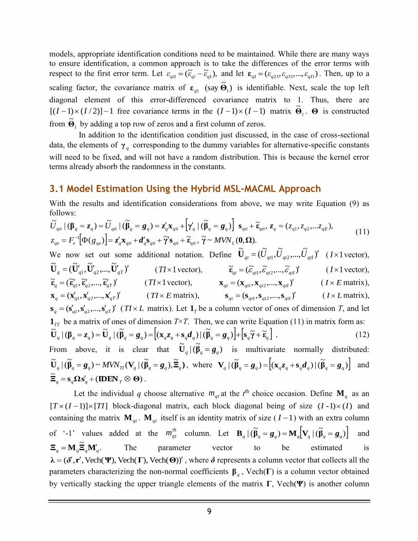
3.1 Model Estimation Using the Hybrid MSL-MACML Approach

With the results and identification considerations from above, we may write Equation (9) as

follows:

).,(~~,~~)(

),,...,(,~)~

(|)~

(|~

)(|~

1

21

Ω0γεsγsx

εsβγxββ

Lqtiqtiqtiqqtiqqeeqe

qEqqqqtiqtiqqqqtiqqqqtiqqqti

MVNgFz

zzzUU

dz

zgzgz (11)

We now set out some additional notation. Define )~

,...,~

,~

(~

21 qtIqtqtqt UUUU ( 1I vector),

)~

,...,~

,~

(~

21 qTqqq UUUU ( 1TI vector), )~,...,~,~(~

21 qtIqtqtqt ε ( 1I vector),

)~,...,~,~(~21

qTqqq εεεε ( 1TI vector), ),...,,( 21 qtIqtqtqt xxxx ( EI matrix),

),...,,( 21 qTqqq xxxx ( ETI matrix), ),...,,( 21

qtIqtqtqt ssss ( LI matrix),

),...,,( 21 qTqqq ssss ( LTI matrix). Let T1 be a column vector of ones of dimension T, and let

TT1 be a matrix of ones of dimension T×T. Then, we can write Equation (11) in matrix form as:

. ~~)~

(|)()~

(|~

)(|~

qqqqqqqqqqqqqq εγsβsxβUβU gdzgz (12)

From above, it is clear that )~

(|~

qqq gβU is multivariate normally distributed:

)ΞβVβU qqqqTIqqq MVN~

),~

(|(~)~

(|~

gg , where )~(|)()

~(| qqqqqqqqq gdzg βsxβV and

)(~

ΘIDENsΩsΞ Tqqq.

Let the individual q choose alternative qtm at the tth choice occasion. Define qM as an

][)]1([ TIIT block-diagonal matrix, each block diagonal being of size )()1-( II and

containing the matrix qtM . qtM itself is an identity matrix of size ( 1I ) with an extra column

of ‘-1’ values added at the th

qtm column. Let )~(|)

~(| qqqqqqq gg βVMβB and

.~

qqqq MΞMΞ The parameter vector to be estimated is

))Vech( ),Vech( ),Vech(,,( ΘΓΨrλ δ , where δ represents a column vector that collects all the

parameters characterizing the non-normal coefficients qβ , Vech(Γ) is a column vector obtained

by vertically stacking the upper triangle elements of the matrix Γ, Vech(Ψ) is another column

10

vector obtained by vertically stacking the upper triangle elements of the matrix Ψ, and Vech(Θ)

is a third column vector obtained by vertically stacking the estimable upper triangular elements

of the matrix Θ. The likelihood contribution of individual q conditional on qq zβ (that is,

qq gβ~

) is as below:

, ,)~

(|)~

(|)()(|)( ~**

ΞβBβλβλ qqqqJqqqqqq LL ggz (13)

where ),1(~

ITJ ),~

(|)~

(| 1

Ξ qqqqqq qgg

βBωβB*

,1

Ξ

1

Ξ

qq qq ωΞωΞ

* and

qΞω is the

diagonal matrix of standard deviations of qΞ . Finally, the unconditional likelihood contribution

of individual q is:

, );( ,)~

(|)( , )~

(|)( ~~~ dg ggdzgβEqqqqJ

g

g

EqqqqJ

z

z

q fL ΓΞβBzΞβBλ****

(14)

where );( ~βE Γ g is the E-variate multivariate standard normal density function with correlation

matrix β~Γ , and evaluated at the vector g.4 The reader will note that the vector δ of the moment

parameters characterizing the non-normal coefficients qβ appears in the above function through

)~

(| qqq gβB* , which itself is a function of )~

(|)()~

(| q qqqqqqqq gdzg βsxβV . In the

latter expression, each element of the vector qz is computed as )(1

qeeqe gFz during the

integration over the vector qg in Equation (14), and the parameters comprising δ feature in the

inverse function 1

eF (.). Thus, the proposed copula model allows consideration of a whole

variety of non-normal multivariate random coefficient distributions, though using distributions

that have a closed-form inverse function make the computation easier than when there is no

closed-form. Importantly, the elements of the vector βq can have different non-normal

distributions. The support of each non-normal element can range from the entire real line to only

the positive (or negative) half-line. While there are many distributions that have support on the

entire real line, Table 1 provides a sample list of univariate marginal distributions that may be

considered for elements that are strictly restricted to the positive half-line, have at least the first

and second inverse moments that exist (important for willingness to pay computations where an

element appears in the denominator of a ratio), and have closed-form inverse (or quantile)

functions.

4 Note that, by construction, the marginal multivariate distribution function of β

q is the multivariate standard normal

distribution function of qβ

~; that is ),;()( ~

βqEqqEF Γzβ g from which

,);( )(

)( ~

q

q

βqE

q

qqE

qE

dFf

dz

dg g

dΓ

z

zβz

or

qβqEqqEf dg gdz );()( ~Γz , and Equation (14) is the result.

11

Table 1: Sample distributions with closed-form inverse cumulative distribution functions and that are bounded on the half-line

Distribution

Name

Density Function

𝑓𝛽𝑞𝑒(𝑍𝑒) = Prob[𝛽𝑞𝑒 = 𝑍𝑒]

Cumulative Distribution

Function

𝐹𝛽𝑞𝑒(𝑍𝑒) = Prob[𝛽𝑞𝑒 < 𝑍𝑒]

Inverse CDF

𝐹𝛽𝑞𝑒

−1 (𝑔𝑒) General Notes

Exponential 1

𝜎𝑒−(

𝑍𝑒− 𝜇𝜎

) 1 − 𝑒−(

𝑍𝑒− 𝜇𝜎

) −𝜎 ln(1 − 𝑔𝑒) + 𝜇

𝑧𝑒 ≥ 0, 𝜎 > 0, 𝜇 ≥ 0

Mean = 𝜎 + 𝜇, Median = 𝜎ln (2) + 𝜇, Mode = 𝜇, Range: 𝜇 to ∞, Std. Dev = 𝜎, All inverse moments exist if 𝜇 > 0

No inverse moments exist if 𝜇 = 0

Rayleigh (𝑍𝑒 − 𝜇

𝜎2) 𝑒

−[12

(𝑍𝑒− 𝜇

𝜎)

2] 1 − 𝑒

−[12

(𝑍𝑒− 𝜇

𝜎)

2]

𝜎√−2ln (1 − 𝑔𝑒) + 𝜇

𝑧𝑒 ≥ 0, 𝜎 > 0, 𝜇 ≥ 0

Mean = 𝜎√𝜋

2+ 𝜇,

Median = 𝜎√2ln (2) + 𝜇,

Mode = 𝜎 + 𝜇, Range: 𝜇 to ∞,

Std. Dev = 𝜎√4 − 𝜋

2,

All inverse moments exist if 𝜇 > 0

No inverse moments exist if 𝜇 = 0

Weibull (𝛾

𝛼) (

𝑍𝑒 − 𝜇

𝛼)

𝛾−1

𝑒−[(

𝑍𝑒− 𝜇𝛼

)𝛾

] 1 − 𝑒

−[(𝑍𝑒− 𝜇

𝛼)

𝛾]

𝛼[−ln (1 − 𝑔𝑒)]1

𝛾⁄

+ 𝜇

𝑧𝑒 ≥ 0, 𝜎 > 0, 𝛾 > 0, 𝜇 ≥ 0

Mean = 𝜎Γ(𝛾−1 + 1) + 𝜇,

Median = 𝜎[ln (2)]1

𝛾⁄ + 𝜇,

Mode = {= 𝜇 𝑖𝑓 0 < 𝛾 ≤ 1

= 𝛼[(1 − 𝛾−1)]1

𝛾⁄ + 𝜇 𝑖𝑓 𝛾 > 1,

Range: 𝜇 to ∞, Std. Dev = 𝜎[Γ(1 + 2𝛾−1) − {Γ(1 + 𝛾−1)}2],

Γ(𝑎) = ∫ 𝑡𝑎−1𝑒−𝑡𝑑𝑡∝

𝑡=0

All inverse moments exist if 𝜇 > 0

Inverse 𝑘𝑡ℎ inverse moments exist if 𝜇 = 0 and 𝛾 > 𝑘

If 𝛾 = 1, Weibull collapses to exponential

If 𝛾 = 2, Weibull collapses to Rayleigh with 𝛼 = √2𝜎

12

Distribution

Name

Density Function

𝑓𝛽𝑞𝑒(𝑍𝑒) = Prob[𝛽𝑞𝑒 = 𝑍𝑒]

Cumulative Distribution

Function

𝐹𝛽𝑞𝑒(𝑍𝑒) = Prob[𝛽𝑞𝑒 < 𝑍𝑒]

Inverse CDF

𝐹𝛽𝑞𝑒

−1 (𝑔𝑒) General Notes

Log-

Normal

1

𝑍𝑒𝜎 𝜙 (

ln𝑍𝑒 − 𝜇

𝜎) Φ (

ln𝑍𝑒 − 𝜇

𝜎) 𝑒[𝜎𝜙−1(𝑔𝑒)+𝜇]

𝑧𝑒 ≥ 0, 𝜎 > 0

Mean = 𝑒(𝜇+12

𝜎2), Median = 𝑒𝜇

Mode = 𝑒𝜇−𝜎2,

Range: Strictly positive Real line,

Std. Dev = 𝑒𝜇√𝑒𝜎2(𝑒𝜎2

− 1),

All inverse moments exist

Power Log-

Normal

(𝑝

𝑍𝑒𝜎) 𝜙 (

ln𝑍𝑒 − 𝜇

𝜎)

{Φ [− (ln𝑍𝑒 − 𝜇

𝜎)]}

𝑝−1

1 − {Φ [− (ln𝑍𝑒 − 𝜇

𝜎)]}

𝑝

𝑒[−𝜎Φ−1[(1−𝑔𝑒)

1𝑝⁄ ]+𝜇]

𝑧𝑒 ≥ 0, 𝜎 > 0, 𝑝 > 0

Mean = ∫ 𝑒[−𝜎Φ−1(𝑦

1𝑝⁄ )+ 𝜇]

𝑑𝑦1

0

,

Median = 𝑒[−𝜎Φ−1{0.51

𝑝⁄ }+𝜇]

Mode is solution to: 1 + (ln𝑍𝑒 − 𝜇

𝜎2)

+ (𝑝 − 1

𝜎) ϕ (

ln𝑍𝑒 − 𝜇

𝜎) [Φ {− (

ln𝑍𝑒 − 𝜇

𝜎)}]

−1

= 0

Range: Strictly positive Real line,

Std. Dev = √[{∫ 𝑒[−2𝜎Φ−1(𝑦

1𝑝⁄ )+ 𝜇]

1

0

𝑑𝑦} − Mean2],

If 𝑝 = 1, power lognormal collapses to lognormal

13

Of these, we would particularly like to bring attention to the last of these distributions – the

power log-normal distribution that has received little attention in the statistical literature and no

attention at all in the context of coefficient distributions in discrete choice models. The

advantage we see in this distribution relative to other distributions (including the log-normal) is

that it can both allow for substantial heterogeneity (large variance parameter) while also ensuring

that the skewed tail is relatively thin. This helps because convergence during estimation is much

easier.5 Figure 1 shows a comparison of the log-normal and the power log-normal for identical

values of μ and σ, but with different values of p in the power log-normal (when p=1 in the power

log-normal, it collapses to the log-normal). Figure 1 plots the power log-normal only for p>1,

which leads to thinner tails than the log-normal. The constraint p>1 can be maintained by

reparametrizing p as ).~exp(1 pp In this sense, the power log-normal with p>1 is like the

skew-normal in that it creates skew while keeping the tails thin.

Figure 1: Comparison of the log-normal (p=1) and the power log-normal distributions for

identical values of µ and σ (µ=0 and σ=1)

5 On the other hand, the problem with the log-normal distribution to represent a coefficient such as a cost coefficient

is that the tails of the distribution are directly determined by the variance term. If there is high heterogeneity in the

sensitivity to cost, this immediately implies a peaking (mode) close to zero as well as a long and fat left tail (note

that the cost coefficient is introduced as the negative of the log-normal distribution). The result is that, as the

variance parameter of the log-normal distribution increases (for the same mean parameter), a larger fraction of

individuals will have a small cost coefficient. At the same time, a small fraction of individuals will have very high

cost sensitivity because of the long and fat tail. The result can cause unusually large and small willingness to pay

estimates. Further, the long and fat tail on the unbounded side of the distribution is known to cause convergence

problems during estimation (Bartels et al., 2006).

14

The simulation approaches for evaluating the full likelihood function in Equation (14)

involve integration of dimension ,)1( EIT which can explode quickly as the number of

choice occasions of the same individual increases (in the case of a cross-sectional model with

only one observation per individual, T=1, and the integral dimensionality is only ).)1( EI

However, one can consider the following (pairwise) composite marginal likelihood function

formed by taking the products (across the T choice occasions) of the joint pairwise probability of

the chosen alternatives qtm for the tth choice occasion and tqm for the tth choice occasion for

individual q.

)()(1

1 1

,, λλ

T

t

T

tt

tqtCMLqCML LL , (15)

where

,);( ~

, )~

(|~

)( ~, qβqEtqtqqtqtJ

g

g

tqtCML

q

q

L dg gg*

ΓΞβBλ*

(16)

where )1(2 IJ

, ,~

,)~

(|)~

(|~ * '**

ΔΞΔΞβBΔβB tqtqtqttqtqqqtqtqqtqt *gg and tqt Δ is a JJ

~*

-

selection matrix with an identity matrix of size ( 1I ) occupying the first ( 1I ) rows and the

thIt 1)1()1( through thIt )1( columns, and another identity matrix of size ( 1I )

occupying the last ( 1I ) rows and the thIt 1)1()1( through thIt )1( columns. All

other elements of take the value of zero. The pairwise likelihood function now only needs

the evaluation of a EI )1(2 -dimensional integral. Note also that, in a cross-sectional

model (T=1), the CML likelihood function of Equation (15) has no pairings to consider and

effectively collapses to the full likelihood function of Equation (14), involving the evaluation of

an EI )1( -dimensional integral. Finally, it is important to note that the same draws have to

be used for the integration over qg across all pairings corresponding to the same individual q.

The properties of the general CML estimator may be derived using the theory of

estimating equations (see Bhat, 2014). Under usual regularity conditions, the maximization of

the logarithm of the CML function, where the CML function across all the Q individuals is

Q

q

qCMLCML LL1

, )()( λλ , is achieved by solving the composite score equations that are

themselves linear combinations of valid likelihood score functions associated with the event

probabilities forming the composite log-likelihood function. Thus, the score equations

immediately satisfy the requirement of being unbiased. Further, with q independent observations

with panel data or repeated choice data, in the asymptotic scenario that Q , a central limit

theorem and a first-order Taylor series expansion can be applied in the usual way (see, for

example, Godambe, 1960) to the resulting mean composite score function to obtain consistency

and asymptotic normality of the CML estimator (see Section 1.4 of Bhat, 2014).

tqt Δ

15

The covariance matrix is estimated as:

,

ˆˆˆˆ

QQ

1-1-

1-

HJHGwith

CMLCML

Q

q

T

t

T

tt

tqtCMLQ

q

qCML L

Q

L

Qλ

1

1

1 1

,

2

λ1

,

2 )log1)log1ˆ

λλ

(λ

λλ

(λH

CML

CML

T

t

T

tt

tqtCMLT

t

T

tt

tqtCMLQ

q

qCMLqCMLQ

q

LL

Q

LL

Q

λ

1

1 1

,1

1 1

,

1

λ

,,

1

)log)log1

)log)log1ˆ

λ

(λ

λ

(λ

λ

(λ

λ

(λJ

(17)

An alternative estimator for H is as below:

Q

q

T

t

T

t

tqtCMLtqtCML

CML

LL

Q 1

1

1 1λ

,, )log)log1ˆλ

(λ

λ

(λH

In the special case of a cross-sectional model, there are no pairings to consider and the

covariance matrix collapses to the traditional inverse of the sandwich information matrix.

There are two final issues. The first is that the covariance matrices Γ and 1

~Θ have to be

positive definite. The simplest way to ensure the positive-definiteness of these matrices is to use

a Cholesky-decomposition and parameterize the CML function in terms of the Cholesky

parameters (rather than the original covariance matrices). Also, the matrix Γ is a correlation

matrix, which can be maintained by writing each diagonal element (say the aath element) of the

lower triangular Cholesky matrix of Γ as

1

1

21a

j

ajl , where the ajl elements are the Cholesky

factors that are estimated. Using these Cholesky-parameterization, the parameters to be estimated

in the model may be written as: ,))Vech(),Vech(),Vech(,,( ΘΓ LLΨrλ δ where ΓL is the

parameterized (as above) lower Cholesky matrix of the matrix Γ and ΘL represents the lower

Cholesky matrix of the estimable parameters of 1

~Θ (as indicated earlier, Θ is constructed from

1

~Θ ).

The second issue relates to the starting parameters. In our experimentation of alternative

procedures to arrive at good starting values, the following procedure worked well: (a) Assume a

kernel error term covariance matrix that corresponds to an IID error structure across the

alternatives with a variance of one-half for each alternative error term), (b) Estimate the

parameters characterizing the marginal non-normal and normal coefficients, fixing the

parameters of the copula correlation matrix and the kernel covariance matrix to their starting

values discussed above, and (c) Use the coefficient vector from the estimation results in step (b)

to begin the iterations for the overall estimation of the model system.

16

3.2 Alternative Estimation Procedure

An alternative estimation procedure is to develop the likelihood function for each individual

conditional on both the qq γβ and vectors, and then integrate both out at the end (as opposed to

the procedure in the previous section of first writing the conditional likelihood given qβ and then

integrating out qβ ) . In this alternative procedure, using the earlier definitions, we first write

qtqtqtqqqtqqqt εsxγβUγβU ~ )~,~

(|~

),(|~

wzwgwz* . Next, defining

wz qtqtqt sxA ~

, ,~

qtqtqt AMA qtqt MΘMΘ

, ,1

Ξ qtqt qAωA

* ,11 ΘΘ

ωΘωΘ

* the likelihood

function at choice occasion t conditional on )~,~

,isthat(and *wgwz qqqq γβγβ is

,,)~ ,~

(|))~,~

(|)(),(|)( )1(

**ΘγβAγβλγβλ

**wgwgwz qqqtIqqqtqqqt LL

and the individual-level likelihood function is:

.);,( ,)~,~

(|)(

*

* 1

)1(

***dgdw wgw g ΓΘγβAλ

**

E

g

g

w

w

T

t

qqqtIqL

(18)

The above function involves the evaluation of an E+L-dimensional outer integral followed by

evaluations of ( 1I )-dimensional orthant inner integrals.

In the cross-sectional case, the estimation procedure from Section 3.1 is much more

computationally efficient. This is because the estimation procedure from earlier exploits the fact

that the conditional distribution of a subset of multivariate normally distributed coefficients

involved in a copula-generated larger multivariate distribution, given the subset of non-normally

distributed coefficients, is also multivariate normally distributed. To our knowledge, this is the

first time this specific property of the multivariate Gaussian copula has been exploited in the way

we do. Then, the conditional multivariate normal distribution of coefficients is combined with

the kernel error multivariate normal distribution, so that the resulting multivariate normal

distribution of the utilities (conditional on the non-normally distributed coefficients) has the

same dimensionality as the kernel distribution of the utility error terms (that is, 1I ). This leads

to a reduction by L (the number of normally distributed coefficients) in the dimensionality of

integration in the earlier estimation procedure than the one in the current section. As importantly,

as indicated earlier in this report, as the number of dimensions for integration increases,

convergence problems arise in the MSL approach and the time for convergence increases

substantially. On the other hand, by using the MSL approach only for the non-normal

coefficients (which tend to be very few in number in most applications), and using a smooth

analytic evaluation approach for the ( 1I )-dimensional orthant multivariate distribution

function (as we propose and implement in this report using Bhat’s MACML approach),

convergence problems get reduced as does the computational time.

In the panel case, the full information likelihood of Equation (14) in Section 3.1 becomes

difficult to impractical as the number of choice occasions per individual (i.e., T) increases.

However, the CML of Equation (16) in the previous section still retains substantial advantages

compared to the MSL estimation technique of this section in Equation (18). This is because of

three reasons. First, the 2)1( I orthant multivariate probability in Equation (16) is

conveniently computed using the MACML procedure, which breaks this multivariate probability

into solely bivariate and univariate cumulative normal distribution function computations (Bhat,

2011). Second, having a well behaved and smooth analytic expression as the integrand over

17

which only a few non-normally distributed coefficients need to be integrated will generally lead

to much superior convergence and computational properties rather than the alternative of

simulating over all normal and non-normally distributed coefficients. Third, when the number of

choice occasions increases, the result is that the integrand in Equation (18) becomes smaller and

smaller (because it is the product of probabilities over all choice occasions), leading to potential

problems in convergence (artificial scaling approaches may be devised to keep the integrand

from getting too small, but this has limited use as the number of choice occasions increases). On

the other hand, the CML of Equation (16) does not have this problem, because the logarithm of

this equation leads to summations outside the 2)1( I -dimensional integral. But the CML of

Equation (16) also involves more and more pairings as the number of choice occasions increases.

Fortunately, one can use a different CML function than that in Equation (16) in such cases.

Specifically, instead of taking all pairings, one can develop a CML function that only includes a

specified number of randomly chosen choice occasions (say T ) to form the pairings, while

leaving the others independent. For ease in presentation, assume that the choice occasions are

ordered so that the randomly chosen T pairings appear first for each individual. Then, the

individual-level contribution to the CML is:

)()()(~

1

,

1

1 1

,, λλλ

T

Tt

qtCML

T

t

T

tt

tqtCMLqCML LLL (19)

where )(, λtqtCMLL is defined as earlier, and

dg gg* );( ,)

~(|)(

β~)1(, ΓΞβBλ

*

EqtqqtI

g

g

qtCMLL

, (20)

with ,,)~

(|)~

(| * '**ΔΞΔΞβBΔβB qtqqtqtqqqtqtqt

*gg and qtΔ

is a JI

~*)1( -selection matrix

with an identity matrix of size ( 1I ) occupying the first ( 1I ) rows and the

thIt 1)1()1( through thIt )1( columns. All other elements of qtΔ

take the value of

zero. The covariance matrix is estimated as in Equation (17), with the following substitutions:

CML

Q

q

T

Tt

qtCMLT

t

T

tt

tqtCML LL

Qλ

1 1

,

21

1 1

,

2 )log)log1ˆ

λλ

(λ

λλ

(λH

CML

qCMLqCMLQ

q

LL

Qλ

,,

1

)log)log1ˆ

λ

(λ

λ

(λJ (21)

CML

T

t

T

tt

T

Tt

qtCMLtqtCMLT

Tt

qtCMLT

t

T

tt

tqtCMLQ

q

LLLL

Qλ

1

1 1 1

,,

1

,1

1 1

,

1

)log)log)log)log1

λ

(λ

λ

(λ

λ

(λ

λ

(λ

An alternative estimator for H is as below:

CML

Q

q

T

Tt

qtCMLqtCMLT

t

T

t

tqtCMLtqtCML LLLL

Qλ

1 1

,,1

1 1

,, )log)log)log)log1ˆ

λ

(λ

λ

(λ

λ

(λ

λ

(λH

18

Chapter 4. Simulation Evaluation

Simulations were performed for two different distributional configurations of random

parameters. In both set-ups, we consider a cross-sectional mixed MNP model with four

alternatives and three independent variables (a panel mixed MNP is considered in the empirical

analysis). The values of each of the three independent variables for the alternatives are drawn

from a standard univariate normal distribution. Once drawn, the exogenous variables are held

fixed for the data set. We generate a sample of 3000 realizations of the three independent

variables corresponding to a situation of 3000 choice occasions.

We allow random coefficients on all the three independent variables. In the first set of

simulations, two of the three coefficients are assumed to be realizations from power log-normal

distributions with identical location parameters ( 1 and 2 =0.5), identical scale parameters ( 1

and 2 =1.0), and identical power terms ( 1p and 2p = 5, considered fixed).6 The last coefficient

is assumed to be a realization from a normal distribution with mean r = 0.5 and standard

deviation η = 1.5. In the second set of simulations, the three coefficients are assumed to be

realizations of different distributions: power log-normal ( 1 =0.5, 1 =1.0 and 5p ),

exponential ( 2 =1.0 and 2 =0.8) and normal ( r = 0.5 and =1.5) respectively. In both cases

all the parameters except for p are freely estimated. The reason for testing two settings of

simulations with different distributional configurations is to evaluate the performance of the

model in recovering parameters vis-à-vis different distribution shapes (tail length).

To ensure the positivity of the scale parameters 1 and 2 , we parameterize them as

2,1),~exp( jjj in estimation. The first two random coefficients in the above setup

constitute the βq vector in the notation of Chapter 3, with ),,,,( 22111 pδ . The normal

distribution scale parameter for the third coefficient is also parameterized as )~exp( in

estimation (technically, because of the symmetric nature of the normal distribution, one can let

the standard deviation to be free, and simply change the sign if it is estimated to be negative; but

we prefer the parametrization from the beginning to help the optimization process along a single

line search direction). In the notation of Section 2.1, )(rr and ).()Vech( Ψ All of these

coefficients are tied together through the dependency (correlation) matrix of the Gaussian

copula. The correlation structure used in the first and in the second sets of simulations is as

follows:

6 As discussed earlier, the log-normal distribution a priori fixes the power term to 1. Here, while we can estimate

the power term, our experience suggested that the optimization algorithms took longer with much more convergence

difficulty than if the power term was fixed. That is, the best way to estimate a model with a power log-normal term

appears to be to estimate the model at different fixed values of the power term, and then compare the data fits across

the different optimization function values (corresponding to different fixed values of the power term) to determine

the best value for the power term. That is the reason we fix the power term at the value of three in the simulation

estimations here, while estimating the means (μ1 and μ2) and the scale parameters (σ1 and σ2).

19

894.00000.00000.0

200.0800.00000.0

400.0600.00000.1

894.0200.0400.0

000.0800.0600.0

000.0000.0000.1

0.14.04.0

4.00.16.0

4.06.00.1

1) ΓΓLLΓ

697.00000.00000.0

393.0917.00000.0

600.0400.00000.1

697.0393.0600.0

000.0917.0400.0

000.0000.0000.1

0.16.06.0

6.00.14.0

6.04.00.1

2) ΓΓLLΓ

Again, as indicated earlier, to maintain positive definiteness, we work with the Cholesky

decomposition elements of the correlation matrix of the Gaussian copula. Thus, there are three

Cholesky matrix elements to be estimated in ΓL corresponding to the non-diagonal elements in

the matrices above (note that the diagonal elements are simply a function of the non-diagonal

elements and are not estimated directly, because Γ is a correlation matrix with unit diagonals).

Collectively, then, )2.0,4.0,6.0(),,()Vech( 321 ΓΓΓΓ lllL for the first set and )393.0,6.0,4.0(

for the second set. The important point to note is that the specification above generates

dependence across the different distributions.

With the preliminaries above, the vector ),( qqq γβα is generated as follows for the

first case in which two of the coefficients follow a power lognormal distribution and the third

follows a normal distribution: (a) First draw a three-variate realization of )~,~

( qq γβ from the

multivariate standard normal distribution of three dimensions with a mean vector of all zero

elements and correlation matrix Γ, (b) Obtain the realization of qj as

2,1,)~

(1exp)~

(/111

1 jF j

p

qjjqj , (c) Obtain the realization of the one-

dimensional vector qγ as rγΨγ qq~ ,where Ψ is the one-dimensional (in this simulation case)

diagonal matrix with the element η as the scale parameter, and r is the one-dimensional mean

location parameter. For the second case where the first coefficient follows a power lognormal

distribution and the second coefficient follows an exponential distribution, the same procedure as

above is followed to generate the first coefficient (the power lognormal) and the third coefficient

(the normal). But the second coefficient 2q is developed from the normal draw 2

~q as follows:

.)~

(1ln)~

( 2222

1

2

qqF

In both simulation settings, we allow a general covariance matrix for the kernel error

term vector qε~ with a covariance specification for Θ as follows:

20

0998000.0000.0000.0

404.0866.0000.0000.0

500.0500.0000.1000.0

000.0000.0000.0000.0

998.0404.0500.0000.0

000.0866.0500.0000.0

000.0000.0000.1000.0

000.0000.0000.0000.0

413.1600.0500.0000.0

600.0000.1500.0000.0

500.0500.0000.1000.0

000.0000.0000.0000.0

ΘΘLL

Θ

Note that, as discussed in Chapter 3, the first row and first column are all normalized to zero, and

the second diagonal element is normalized to 1 for identification. To maintain positive

definiteness, we work with the Cholesky decomposition elements of Θ, with two Cholesky

matrix elements to be estimated in ΘL = ).998.0and404.0( 65 ΘΘ ll 7 Collectively,

.),()Vech( 65 ΘΘΘ llL A multivariate draw of qε

~ is obtained by drawing I multivariate normally

distributed random numbers in the usual way, given that ),0(MVN~~1 ΘIDENε q for the

cross-sectional case.

To generate the dependent variable values in the simulation for given independent

variable values for each individual (that is, for given qq sx and values), we track back to the

matrix form of Equation (9) and write:

. ~~qqqqqq εγsβxU

Once the multivariate realizations of ),( qqq γβα and qε~ are drawn, the utility of each

alternative at each choice occasion is computed, and the alternative with the highest utility at

each choice occasion is then identified as the chosen alternative.

The above data generation process is undertaken, for each simulation setting, 200 times

with different realizations of the qα and qε~ vectors to generate 200 different data sets, each with

3000 choice occasions as mentioned earlier. The hybrid MSL-MACML inference approach of

Equation (14) is applied to each of the 200 data sets to estimate data specific values of λ. In this

approach, MSL is used to integrate out the non-normal coefficients and for this procedure we use

50 draws per individual from the Halton sequence. The MACML approach is employed to

evaluate the MVNCD function that is the integrand in Equation (14). In the MACML procedure,

a single random permutation is generated for each individual (the random permutation varies

across individuals, but is the same across iterations for a given individual), and the multivariate

normal cumulative distribution (MVNCD) function is approximated using the resulting

conditional probability sequence.

7 The specification for the differenced covariance matrix above may be viewed as being derived from a specification

where the error terms for the first three alternatives are independent and distributed with a variance of 0.5, while the

last error term has a variance of 0.913 and is correlated with the error term of the third alternative with a covariance

of 0.1. In the simulation experiment estimations, to focus on the random coefficients, we fix the variances of the first

three alternatives to 0.5 and impose independence among the first three alternatives, but estimate the variance of the

fourth error term and the covariance between the third and fourth alternatives, which translates to the two Cholesky

parameters .998.0and404.0 65 ΘΘ ll

21

4.1 Performance Evaluation

For both simulation settings, the performance of the hybrid MSL-MACML approach in

recovering parameters of the model is evaluated as follow.

(1) Estimate the parameters for the 200 datasets. Estimate the standard errors.

(2) Compute the mean estimate for each model parameter across the 200 data sets. Compute

the absolute percentage bias (APB) as: 100 valuetrue

valuetrue-estimatemean APB .

(3) Compute the standard deviation of each parameter estimate across the 200 datasets, and

label this as the finite sample standard deviation or FSSD (essentially, this is the

empirical standard error). Compute the FSSD as a percentage of the true value of each

parameter.

(4) Compute the mean standard error for each model parameter across the 200 datasets, and

label this as the asymptotic standard error or ASE (essentially this is the standard error

of the distribution of the estimator as the sample size gets large, and is a theoretical

approximation to the FSSD).

(5) Next, to evaluate the accuracy of the asymptotic standard error formula for the finite

sample size used, compute the absolute percentage bias of the asymptotic standard

error (APBASE) for each parameter relative to the corresponding finite sample standard

deviation.

100FSSD

FSSD-ASEAPBASE

4.2 Simulation Results

Summaries of the performance measures for the first and the second simulation settings are

presented in Table 2 and Table 3, respectively. The tables provide the true value of the

parameters, followed by the parameter estimates and the standard error estimates. Overall, the

results show that the proposed method recovers parameters very well with the average of the

absolute percentage bias (APB) in both cases being lower than 5% (see the last row under the

APB column). Further, the asymptotic standard error from the method also quite closely reflects

the finite sample standard deviation, as evident from the APBASE estimates, whose average

(across all parameters) is less than 9% (see last row under the APBASE column).

22

Table 2: Simulation results for 200 samples of 3000 observations:

Two power log-normal and one normal random parameter

Parameter True value

Parameter Estimates Standard Error

Mean

Estimate APB ASE FSSD APBASE

Power log-normal

1 0.500 0.475 5.09% 0.163 0.164 0.92%

2 0.500 0.467 6.53% 0.165 0.164 1.02%

1 1.000 0.986 1.38% 0.178 0.171 4.51%

2 1.000 0.972 2.82% 0.184 0.169 8.54%

Normal r 0.500 0.491 1.75% 0.070 0.065 7.29%

1.500 1.495 0.37% 0.139 0.128 8.63%

Copula Correlation

1Γl 0.600 0.592 1.34% 0.184 0.160 15.44%

2Γl 0.400 0.381 4.63% 0.111 0.129 14.07%

3Γl 0.200 0.236 18.19% 0.158 0.132 19.72%

Kernel Covariance 5Θl 0.404 0.413 2.29% 0.149 0.168 11.27%

6Θl 0.998 0.980 1.80% 0.101 0.094 7.42%

Overall Average - - 4.20% 0.146 0.140 8.98%

Table 3: Simulation results for 200 samples of 3000 observations:

One power log-normal, one exponential and one normal random parameter

Parameter True value

Parameter Estimates Standard Error

Mean

Estimate APB ASE FSSD APBASE

Power log-normal 1 0.500 0.502 0.45% 0.156 0.152 2.82%

1 1.000 1.000 0.00% 0.167 0.162 3.29%

Exponential 2 1.000 1.013 1.28% 0.119 0.126 6.09%

2 0.800 0.792 1.05% 0.281 0.209 34.48%

Normal r 0.500 0.498 0.47% 0.074 0.070 5.95%

1.500 1.504 0.26% 0.138 0.139 0.25%

Copula

Correlation

1Γl 0.400 0.441 10.22% 0.213 0.178 19.65%

2Γl 0.600 0.604 0.60% 0.095 0.101 6.18%

3Γl 0.393 0.394 0.20% 0.155 0.141 9.99%

Kernel Covariance 5Θl 0.404 0.393 2.66% 0.164 0.165 0.64%

6Θl 0.998 0.973 2.54% 0.106 0.100 5.99%

Overall Average - - 1.80% 0.152 0.140 8.67%

23

Several other observations may be made from the results. In the first setting (the case in

which two coefficients are assumed to be realizations from power log-normal distributions and

one coefficient is assumed to be a realization from a normal distribution; see Table 2), the third

copula correlation parameter )( 3Γl presents a high APB value of 18.19%. However, this result is

rather deceiving because the true estimate for this parameter is 0.20 and the finite sample bias is

only 0.036; that is the APB value is being inflated in percentage simply because of the small

magnitude of the true value of the parameter. Interestingly, this parameter estimate also presents

the highest APBASE value of the table (19.72%). In fact, the APBASE is relatively high for all

the copula correlation parameters relative to other parameters, suggesting that the copula

correlations are the most difficult to precisely estimate. This is not surprising, because the copula

correlation parameters are the ones that occur most non-linearly in the CML function of Equation

(20).

In the second simulation setting (corresponding to the three different distributions of

power log-normal, exponential and normal for the coefficients; see Table 3), the copula

correlation coefficient 1Γl presents the highest APB (10.22%). This represents the correlation

between the power log-normal and exponential distributions. This is to be expected, given the

relatively non-linear and complicated manner in which the copula correlation enters into the

optimization function for retrieving the parameters. This is also reflected in the high APBASE

value (19.65%) for this copula correlation, reinforcing the notion that not only is it difficult to

accurately retrieve this parameter, but so is the precision of recovery of the parameter. But it is to

be noted that even these are not egregiously high biases. The other parameter showing a very

high APBASE (34.48%) is that corresponding to the standard deviation of the exponential

distribution ( 2 ). It is indeed interesting that the two parameters ( 1Γl and 2 ) that are most

difficult to recover (from an accuracy and/or precision standpoint) involve the exponential

distribution. These results are a consequence of the long tail of the exponential distribution, a

reason that also typically makes estimation using a traditional log-normal distribution (that also

has a long tail) rather unstable and imprecise. As in the first simulation setting, we again find that

the copula parameters are the ones that are the most difficult to precisely pin down.

Finally, the copula correlation parameter 2Γl in Table 3, which represents the correlation

between the power log-normal and the normal univariate marginals in the second setting, has a

much smaller APB (0.20%) than 3Γl in the first setting (Table 2), which also represents the

correlation between power log-normal and normal. This result confirms that the high APB of this

parameter in the first setting was due to its small magnitude and not poor recovery.

24

Chapter 5. An Empirical Application

In this chapter, we illustrate the use of the proposed model for an empirical application on a

commuter mode choice dataset containing repeated choices from the same individuals. The

dataset is drawn from a web-based stated preference survey from Austin. The purpose of the

survey was to examine the demographic, employment, and overall travel characteristics of

Austin area commuters, and to identify the possible effects on commute mode share of adding a

commuter rail as a new transportation option. Four alternative modes are presented to the

respondent as commuting options: drive alone, shared ride, bus and the commuter rail. Each

respondent provides the mode she or he would choose to use on four repeated choice occasions,

with different attribute values for each of several attributes, including travel time and travel cost.

Additional details about the survey and the stated preference design can be found in Bhat (2004)

and Bhat and Sardesai (2006). There are 322 individuals in the sample and a total of 1288 choice

occasions. The mode share across all choice occasions is: 45.34% drive alone, 13.43% shared

ride, 5.67% bus and 35.56% commuter rail. While the commuter rail share is very high, the

reader will note that this is purely a stated preference survey in which commuter rail, and the

shared ride and bus modes, were included by design as available options for all individuals, to

maximize the information we were able to extract about the relative tradeoffs between travel

time and travel cost. Besides, for the same reason, the SP choice scenarios involved an increase

over the current scenario for the respondent in drive alone travel times and costs. The obvious

overstatement in non-drive alone mode choice because of the SP design may be controlled for if

one wants to make predictions of future modal shares, as undertaken by Bhat and Sardesai

(2006). But the emphasis in this report is on the distributions of the travel time and cost

coefficients (and the resulting value of time), not on the predictions of modal shares.

5.1 Valuation of Travel Time Savings

The valuation of travel time savings (VTTS) is a central element in transportation planning and

analysis. As indicated by Small (2012), “its theoretical meaning and its empirical measurement

are fundamental to travel demand modeling, social cost analysis, pricing decisions, project

evaluation, and the evaluation of many public policies”. Small proceeds to discuss in detail the

many uses of VTTS, which we will not elaborate on here for presentation conciseness. But the

important point is that, while there is general agreement that no one would be interested in

wasting money on daily travel (such as commuting), it is quite possible that individuals would

want to extend their travel time on at least some travel occasions. Cirillo and Axhausen (2006)

provide a conceptual justification for this in the short term, because, while pure travel time is

valued negatively by individuals, there is a comingling of this (dis-) utility of travel with the

potentially positive utility from secondary activities that may be undertaken during daily travel

(such as being able to listen to relaxing music in the privacy of one’s vehicle, or the joy of being

in movement per se).

For our analysis, it suffices to note that theoretical considerations require that the cost

coefficient (the denominator in the VTTS computation) should be always negative (and cannot

even take the value of zero in its domain, because this causes a singularity problem in the

computation of VTTS). That is, we need a bounded distribution for the cost coefficient that does

not straddle the zero value. However, this need not necessarily be the case for the travel time

coefficient (the numerator in the VTTS computation), especially in the short-term context of

25

daily travel. That is, the travel time coefficient can be unbounded, leading to potentially negative

or zero VTTS values.

In our estimation specifications, we considered several bounded distributions for travel

cost, as well as an unbounded normal distribution and several bounded distributions for travel

time. However, the power log normal distribution (with p=5) consistently came out to be the best

bounded distribution in our empirical context, for both the cost and time coefficients. For

completeness, in the next section, we present the results for all possible combinations of fixed,

log-normal (the distribution that has been typically used in the literature for bounded

distributions), and power log-normal coefficients (with p=5) for cost and time, supplemented by

a possible normal distribution for travel time (but not for cost). This leads to the presentation of

twelve models with different distributional combinations for the cost and time coefficients. In

each of these models, the cost variable is used as cost over personal income. That is, the cost

coefficient is actually a coefficient with the stipulated distribution divided by personal income.

We use such a specification because it is intuitive and also because it came out to be consistently

superior to the simple cost specification. In addition, we tested for a random covariance structure

for the baseline constants (except for one alternative, which is the base alternative) to capture

heterogeneity across individuals in modal preferences (as well as individual-level dependence in

the unobserved modal preferences). The repeated nature of our data allows such an individual-

level covariance structure in modal preferences in addition to the choice occasion-level

heterogeneity captured by the covariance of the choice-occasion-level kernel-error terms. But we

have only four choice occasions per individual, which can be inadequate to tease out a full

covariance matrix capturing inter-individual intrinsic preference differences. In any case, in our

analysis, this generic individual-level covariance terms consistently turned out to be statistically

insignificant whether or not the time and cost coefficient heterogeneities were introduced. And

the fit of the model with only the generic individual-level covariance structure was worse than

the model with only heterogeneity in the cost or time coefficients. Effectively, the time and cost

variables show a good amount of variation (both across individuals as well as within the choice

occasions of the same individual) because of the SP design, thus allowing individual-level

heterogeneity to be captured on these variables. This is also an efficient way of capturing

individual-level heterogeneity, given the relatively small number of individuals in the sample.

But there is simply not sufficient information it appears to pin down the many covariance terms

characterizing the intrinsic individual-level heterogeneity effects.

Also to be noted here is that, as soon as we introduced any random coefficient (for the

cost and/or the time coefficient), the estimated covariance matrix of the differenced error terms

)~~( q1qiqi1 εεε could not be distinguished from a matrix of ones on the diagonal and 0.5 values

on the off-diagonals. That is, we could not rule out an IID covariance matrix for the original

kernel error terms, and so all the models presented in the next section use an IID kernel

formulation. The implication is that, in the current empirical context, any utility covariances at

the individual-level or at the choice occasion-level may be structurally traced to individual-level

random coefficients in the cost and/or time coefficients.

5.2 Empirical Results

In this section, we first discuss data fit and VTTS considerations, and then present the full model

results for the preferred model specification.

26

5.2.1 Data Fit and VTTS Estimates

The third main column of Table 4 shows the composite marginal likelihood (CML) values at

convergence for the twelve model specifications discussed earlier. The same variable

specification was retained for all the twelve models, with the only difference being in the

distributional assumptions for the cost and time coefficients (indeed, the same set of variables

came out to be appropriate from a statistical significance perspective for all twelve models). The

many models may be compared with each other based either on a nested test (when one model is

a restricted version of the other) or a non-nested test. In Table 4, all the models with a fixed cost

and/or fixed time coefficient are restricted versions of appropriate other models (for example, a

model with a fixed cost coefficient and a normally distributed travel time coefficient is a

restricted version of all models with a specified random distribution on the cost coefficient and a

normally distributed travel time coefficient). In these cases, the restrictive models can be

compared with the corresponding unrestricted models using the adjusted composite marginal

likelihood ratio test (ADCLRT; see Bhat, 2014). However, for all cases of comparisons between

two models with one or both random coefficients with different distributional assumptions, one

needs to use a non-nested statistical test. This can be done using the composite likelihood

information criterion (CLIC) introduced by Varin and Vidoni (2005) may be used. The CLIC

takes the following form8:

1* )ˆ(ˆ)ˆ(ˆ)ˆ(log)ˆ(log θHθJθθ trLL CMLCML (22)

The model that provides a higher value of CLIC is preferred. Technically, the CLIC statistic can

also be used to compare nested models, though it has less power than the ADCLRT statistic. So,

for presentation ease, in Table 4, we only show the CLIC statistic for each of the estimated

models (however, each restricted model was rejected in favor of its unrestricted versions based

on the ADCLRT test).

8 This penalized log-composite likelihood is nothing but the generalization of the usual Akaike’s Information

Criterion (AIC). In fact, when the candidate model includes the true model in the usual maximum likelihood

inference procedure, the information identity holds (i.e., H(θ)=J(θ)) and the CLIC in this case is exactly the AIC

)ˆ(log[ θML

L (# of model parameters)].

27

Table 4: Data fit and Value of Travel Time Savings (VTTS) for different models

Model

Number

Coefficient distribution

Composite

marginal log-

likelihood

(CML) value

at convergence

CLIC

statistic

Median VTTS Value (computed by

simulation using 20,000 bivariate

simulation realizations)

Cost1 Time

Low annual

income

(US

$15,000)

Medium

annual

income

(US

$50,000)

High

annual

income

(US

$150,000)

1 Fixed Fixed -4390.02 -4420.11 8.72 29.08 87.24

2 Fixed Normal -4355.96 -4387.57 10.47 34.89 104.67

3 Fixed Log-normal -4365.14 -4376.27 4.68 15.59 46.78

4 Fixed Power log-normal2 -4364.73 -4375.73 4.56 15.19 45.59

5 Log-normal Fixed -4319.15 -4330.32 4.47 14.89 44.68

6 Log-normal Normal -4281.47 -4294.56 2.91 9.79 29.14

7 Log-normal Log-normal -4300.15 -4313.22 2.44 8.15 24.45

8 Log-normal Power log-normal -4299.58 -4312.79 2.32 7.73 23.18

9 Power log-normal Fixed -4315.64 -4326.65 4.59 15.31 45.92

10 Power log-normal Normal -4277.88 -4290.96 2.47 8.23 24.69

11 Power log-normal Log-normal -4296.69 -4309.71 2.48 8.28 24.85

12 Power log-normal Power log-normal -4296.08 -4309.09 2.30 7.68 23.04

1 The cost variable is introduced in all specifications as cost/personal income. 2 For all Power log-normal distributions p=5.

Several important observations may be made from Table 4. First, the model with fixed

cost and time coefficients (Model 1) is rejected soundly relative to random coefficients on one or

both of travel cost and travel time. This clearly suggests the presence of random individual-level

heterogeneity in taste to cost/time. Second, models with a fixed coefficient on one of the travel

time or travel cost variables (Models 2, 3, 4, 5, and 9) fare much more poorly than models with

both coefficients randomly distributed (Models 6, 7, 8, 10, 11, 12). This finding supports the

notion that it is not advisable to a priori fix a coefficient simply to make WTP computations

easier (see Train and Weeks, 2005, for related reasons for not fixing the cost coefficient). Third,

the results show that the models with a fixed coefficient on travel time and a bounded

distribution on travel cost (models 5 and 9) are superior from a data fit standpoint relative to

those that specify a fixed coefficient on cost and a random coefficient on travel time (models 2,

3, and 4; note that the CLIC statistic ranges from -4320 to -4315 for the first set of models

compared to the range from -4388 to -4374 for the second set of models). The implication is that

there is much more individual-level heterogeneity related to cost sensitivity rather than

associated with time sensitivity. Fourth, between any pair of models with the same distributional

assumption for the travel time coefficient, a power-lognormal distribution for the cost coefficient

does better than the traditional log-normal distribution (compare models 5 versus 9, 6 versus 10,

7 versus 11, and 8 versus 12). As indicated earlier, the proposed model allows a flexible

parametric distributional form for the random coefficients. Our results suggest that researchers

may want to try the power-lognormal as an alternative to the log-normal, especially given

potential convergence problems originating from the long tail of the log-normal. Fifth, the model

28

with a power log-normal cost coefficient distribution and a normal time coefficient distribution

(model 10) provides the best data fit, but also implies that, for some individuals, there is a

positive valuation of travel time, leading to a negative VTTS value. Based on the mean and

standard deviation of the normal travel time coefficient, 29% of individuals are predicted to have

a negative VTTS (this is, interestingly, in the same range as that obtained by Cirillo and

Axhausen, 2006).

Table 4, in addition to providing data fit measures, also provides median VTTS

estimates for three annual personal income categories: low income (US $15,000, the minimum

value in the sample), medium income (US $50,000, the median value), and high income (US

$150,000, a high income value). In the table, we provide the median VTTS estimates because it

is a better central measure to compare across the models. The VTTS median estimate is

computed by drawing 20,000 realizations from the bivariate copula distribution of the time and

cost coefficients, computing the implied VTTS for each bivariate realization by taking the ratio

of the time to cost draws, and then computing the median value across the 20,000 realizations

(for presentation efficiency, we will refer to the median estimate as the VTTS estimate from

hereon), Again, many observations stand out from the VTTS estimates. First, and as expected,

for every model, the VTTS increases proportionally with income, which is a result of the “cost

over income” specification in the models. Second, for each of the three income values, the VTTS

estimate from the model in which both the cost and time coefficients are fixed (model 1) and the

model in which the cost coefficient is fixed and the time coefficient is normally distributed

(model 2) produce the highest estimates. These VTTS estimates are higher than the implied wage

rate for each income category (based on full-time work with 52 weeks and 40 hours per week,

the wage rates for the low, medium, and high income categories are $7.2 per hour, $24 per hour

and $72 per hour). These certainly seem out of the realm of reasonableness. On the other hand,

the lowest VTTS values are obtained in the models that involve a lognormally or power-

lognormally distributed cost coefficient and a random time coefficient (models 6, 7, 8, 10, 11,

and 12). In these models, the VTTS values are about one-third of the wage rate. These models

also have a superior data fit relative to other models. The VTTS estimates for the models with

one fixed coefficient and the other being randomly distributed (models 3, 4, 5, and 9) lie

somewhere in-between, with an implied value of about 63% of the wage rate. Third, a further

exploration of the VTTS distributions (rather than simply the median VTTS estimates) reveals

that there are differences in the distributions even between models providing similar median

VTTS estimates. Thus, among models 6, 7, 8, 10, 11, and 12, which all use a log-normally or

power-lognormally distributed cost coefficient with a randomly distributed time coefficient,

those that use a log-normal distribution for one coefficient and a power-lognormal distribution

for the other (models 7, 8 and 11) belong to one group (labeled Group 1) with a sharp spike in

the VTTS distribution. This is shown in Figure 2, where, to avoid clutter, we show the VTTS

distribution only for model 11 as the representative model for this group (model 11 has the best

data fit in Group 1). The sharp spike for this group is, of course, a manifestation of the log-

normal distribution used for one of the two coefficients. Also, because of the strictly bounded

nature of the distribution for both the cost and time coefficients, we get only positive VTTS

values.

29

* Includes Model 7- Log-normal cost coefficient, Log-normal time coefficient

Model 8- Log-normal cost coefficient, Power log-normal time coefficient

Model 11- Power log-normal cost coefficient, Log-normal time coefficient ** Includes Model 6- Log-normal time coefficient, Normal time coefficient

Model 10- Power log-normal cost coefficient, Normal time coefficient. *** Includes Model 3- Fixed cost coefficient, Log-normal time coefficient

Model 5- Log-normal cost coefficient, Fixed time coefficient

Model 9- Power log-normal cost coefficient, Fixed time coefficient + Includes Model 4- Fixed cost coefficient, Power log-normal time coefficient ++ Includes Model 12- Power log-normal cost coefficient, Power log-normal time coefficient

Figure 2: Resulting VTTS distributions for different groups of models that have random

coefficents for cost or time, or both.

0

0.05

0.1

0.15

0.2

0.25

-2.5 0 2.5 5 7.5 10

Pro

bab

ilit

y D

ensi

ty F

un

ctio

n

VTTS Value

Group 1

Group 2

Group 3

Model 4

Model 12

*

**

***

+

++

30

On the other hand, models 6 and 10, which use a normal travel time coefficient and a log-normal

or power log-normal cost coefficient, also have similar VTTS profiles, but that are very different

from Group 1. In Figure 2, we show the VTTS profile for model 10 as the representative model

for Group 2 comprising models 6 and 10. As should be obvious, this group allows negative

VTTS values (as discussed earlier, of the order of 29% of the distribution) and also has the

lowest spike. Similarly, there are also VTTS distribution differences among the four models with

one fixed coefficient and the other being randomly distributed (models 3, 4, 5, and 9).

Specifically, the VTTS profiles for models 3, 5, and 9 are similar, with that of model 9 shown in

Figure 1 as the representative of this Group 3 set of models. Group 3 is identified by a spike

between that of Groups 1 and 2, and the longest right tail of all groups. Finally, models 4 and 12

also have similar profiles, but are also sufficiently different to be shown separately in Figure 2.

While model 12 uses a power lognormal distribution for both the cost and the time coefficients,

model 4 uses a power lognormal only for the time coefficient with a fixed coefficient on cost

(rendering the VTTS to be power lognormal). The VTTS profiles of both models 4 and 12 start

off similarly on the left edge with a spike of the same order of magnitude, but then the profile for

model 4 moves more toward that of Group 3 with the long tail. This leads to the much higher

median VTTS value from Model 4 compared to model 12. Overall, while different reasonable

analysts can come to different conclusions, we believe that Model 12 represents the best

combination of data fit, median VTTS value as a percentage of wage rate, and the shape of the

VTTS profile. While models 6 and 10 provide a better data fit, the percentage predicted to have a

negative VTTS is just too high in our opinion, as is the implied very high variance across

individuals in their VTTSs. 9

Overall, the results indicate that there needs to be much more emphasis in the literature

on VTTS profiles, rather than simply statistics of the VTTS values such as means, medians, and

standard deviations. The profiles, which play a critical role in consumer welfare analyses, can be

very different even when the imputed VTTS mean or median values are similar. Of course, the

only way that different profiles can be considered is by allowing flexible marginal non-normal

distributions on specific individual coefficients, which is precisely what our proposed copula

model enables the analyst to estimate using a convenient and practically feasible hybrid

MACML-MSL inference technique.

5.2.2 Estimation Results for the Preferred Model (Model 12)

For completeness, Table 5 presents the estimation results for the preferred model, which are

generally consistent with the vast literature now on commute travel mode choice (see, for

example, Bhat and Sardesai, 2006; Paleti et al., 2013; Ho and Mulley, 2015; Wang, 2015). The

alternative-specific constants in the first row panel do not have any substantive interpretations;

9 There has been a healthy discussion and debate in the literature (see, for example, Ory and Mokhtarian, 2005;

Cirillo and Axhausen, 2006) on the issue of whether or not some individuals associate a positive valuation to travel

time as opposed to the predominantly held view that people are averse to higher travel times. Of course, there is also

the issue that this may be very context dependent, including, for example, the length of the travel time being

considered (see, for example, Pinjari and Bhat (2006), who suggest that the sensitivity to travel time is non-linear

over travel time). In this report, we do not engage in this line of debate. The purpose here is to present, and

demonstrate an application of, a flexible copula model and its estimation that can be gainfully employed to estimate

different combinations of multivariate random coefficient distributions to then guide the final model structure and

specification, based on theoretical considerations (for example, which coefficients should have bounded

distributions and which can have unbounded distributions), intuitive considerations (the reasonableness of trade-off

values obtained and their profiles over the population), and statistical data fit considerations.

31

they simply control for the sample values of the exogenous variables and the sample shares,

though the overall negative signs on all the non-drive alone modes are consistent with the high

mode share of the drive alone alternative in the sample. Individuals who earn a higher share of

total household income are less likely to use the currently available non-solo auto modes (share-

ride and bus) relative to those who earn a lower share of total household income, suggesting that

those who wield more market power in the household have “first choice rights” over modes that

are viewed as flexible, fast, and comfortable. Also, non-work activity stops made during the mid-

day and/or during the commute encourage the use of the car mode (either drive alone or shared-

ride). Women are less likely to commute by bus relative to men, though this variable is

statistically significant at only the 83% confidence level. Finally, the table provides the

parameters for the travel cost and travel time distributions, which formed the basis for much of

the discussion in the earlier section. A point that should be noted here is that the copula

parameter came out to be statistically insignificant in the current empirical analysis. But the

situation could be different in other empirical contexts. In any case, the only way to test the

presence and intensity of the copula parameter is to estimate the multivariate Gaussian copula

model introduced in this report.

Table 5: Empirical results of model with power lognormal cost coefficient

and power lognormal time coefficient (coefficients provide the impact of variables on the utility of alternatives)

Variable name Parameter Estimates

Coef. t-stat

Alternative specific constants

Shared ride -0.595 -9.67

Bus -1.160 -10.35

Commuter rail -0.174 -4.16

Personal income divided by household income

Shared ride/Bus -0.263 -3.24

Individual makes non-work mid-day stops

Drive alone 0.072 2.51

Individual makes commute stops

Bus -0.431 -3.83

Commuter rail -0.119 -2.70

Female

Bus -0.130 -1.38

Level of service variables

Trip cost (dollars) divided by personal annual income

(dollars divided by 105)

Mean 1.941 8.16

Standard deviation 2.802 26.98

Travel time (hours)

Mean 2.096 6.29

Standard deviation 2.570 13.16

Copula Correlation 0.120 0.48

32

Chapter 6. Summary and Conclusions

In this report, we propose a mixed multinomial probit model that is able to accommodate

a general covariance structure for the kernel error terms as well as a very flexible continuous

parametric multivariate structure for unobserved individual heterogeneity. The latter is

introduced using a Gaussian copula approach that ties different continuous univariate mixing

distributions into a joint multivariate distribution. The individual univariate mixing distributions

can be bounded or unbounded, allowing the incorporation of theoretical considerations that

require specific coefficients to span only the half-line. In addition, our proposed approach

includes the case of independence across specific coefficients, allows a flexible and wide range

of dependence across coefficients, and is easy to work with. The estimation of the model is

achieved using a combination of the maximum simulated likelihood (MSL) technique (to

accommodate the non-normal random coefficients) and Bhat’s MACML inference approach (to

accommodate all the normal random coefficients as well as the kernel normal error structure; see

Bhat, 2011 and Bhat, 2014). To our knowledge, this is the first time that a copula-based mixed

MNP model has been proposed in the literature, along with an associated hybrid MSL-MACML

inference approach that is ideally suited for the case when there are few non-randomly

distributed coefficients (so that the MSL simulation does not involve very high dimensions) and

many normally distributed coefficients (so that the MACML computational accuracy and

efficiency can be realized). For the non-normal coefficients, the use of univariate distributions

that have a closed-form inverse function facilitates quick estimation. Of these, we would

particularly like to highlight our consideration of the power log-normal distribution that has not

been considered earlier in discrete choice models. The advantage of this distribution relative to

other distributions on the half-line (including the log-normal) is that it can both allow for

substantial heterogeneity (large variance parameter) and also ensure that the skewed tail is

relatively thin, which helps convergence.

We demonstrate the effectiveness of our inference approach through simulation exercises

as well as an empirical application. The simulations involve cross-sectional choice data with a

sample size of 3000, and two configurations of three random coefficients. The first includes two

power log-normal coefficients and one normal coefficient, while the second considers one each

of power log-normal, exponential and normal coefficients. Overall, the simulation results

indicate that the proposed method allows for accurate parameter recovery. Further, the

asymptotic standard errors from the method also quite closely reflect the finite sample standard

deviations. One finding, however, is that it appears to be more difficult to recover the copula

parameters characterizing the dependence between pairs of univariate margins, especially

between pairs of non-normal univariate margins. Also, the simulation results suggest that

distributions with very long tails (such as the exponential and lognormal) make it particularly

difficult to recover variance parameters and corresponding copula parameters of dependence

with other margins. However, even in these cases, the method performs quite well. Future

simulation studies should study the performance of the proposed method in more detail, in

relation to varying sample sizes, both cross-sectional and repeated choice data, different degrees

of copula dependence, an array of different bounded and unbounded univariate margins, and

varying numbers of random coefficients

The empirical application focuses on a repeated choice commute travel mode stated

preference data collected in Austin, Texas. The results reiterate the importance of the power

lognormal distribution as a strong contender (and alternative) to the traditional lognormal

33

distribution and other bounded distributions for the travel cost coefficient. Additionally, the

preferred model with a power lognormal distribution for the cost coefficient (with p=5) and a

power lognormal distribution for the time coefficient yields a median value of travel time savings

that is about a third of the wage rate. Further our results do suggest there is much more

individual-level heterogeneity related to cost sensitivity rather than associated with time

sensitivity.

Of course, the emphasis of this report has been on presenting a new copula-based

discrete choice model structure and an associated inference approach. Much still needs to be

done in terms of investigating ways to obtain good starting parameters for the copula model with

different marginal distributions, and develop structured optimization algorithms for the quick

estimation of models with power lognormal and other margins (for example, is there a better way

to optimize rather than fix p values and estimate different specifications repeatedly, which can

become cumbersome when there are many random coefficients). Besides, additional research

needs to compare the performance and effectiveness of the proposed copula-based model with

other non-parametric ways to introduce taste heterogeneity. There is also room for testing

different distributional assumptions that were not included in this study. For example, future

research should test the use of log-uniform and log-triangle distributions that, similar to the

power log-normal, are bounded above zero and have thin tails that allow for heterogeneity while

facilitating convergence. We hope that this new flexible parametric approach will offer

researchers and practitioners another way of accommodating heterogeneity in a general and

efficient manner in choice models, and open up a new stream of empirical applications with

bounded and non-normal distributions.

34

References

Amador, F.J., Gonzales, R., Ortuzar, J., 2005. Preference heterogeneity and willingness to pay

for travel time savings. Transportation 32(6), 627-647.

Azzalini, A., 2013. The Skew-normal and Related Families (Vol. 3). Cambridge University

Press, Cambridge, U.K.

Balcombe, K., Chalak, A., Fraser, I.M., 2009. Model selection for the mixed logit with Bayesian

estimation. Journal of Environmental Economics and Management 57(2), 226–237.

Bartels, R., Fiebig, D.G., van Soest, A., 2006. Consumers and experts: an econometric analysis

of the demand for water heaters. Empirical Economics 31(2), 369-391.

Bastin, F., Cirillo, C., Toint, P.L., 2010. Estimating nonparametric random utility models with an

application to the value of time in heterogeneous populations. Transportation Science

44(4), pp.537-549.

Berry, S.T., Haile, P.A., 2014. Identification in differentiated products markets using market

level data. Econometrica 82(5), 1749-1797.

Bhat, C.R., 1997. Work travel mode choice and number of non-work commute stops.

Transportation Research Part B 31(1), 41-54.

Bhat, C.R., 2004. Austin commuter survey: findings and recommendations. Technical Report,

Department of Civil, Architectural & Environmental Engineering, The University of

Texas at Austin.

http://www.ce.utexas.edu/prof/bhat/reports/austin_commuter_survey_report.doc

Bhat, C.R., 2011. The maximum approximate composite marginal likelihood (MACML)

estimation of multinomial probit-based unordered response choice models.

Transportation Research Part B 45(7), 923-939.

Bhat, C.R., 2014. The composite marginal likelihood (CML) inference approach with

applications to discrete and mixed dependent variable models. Foundations and Trends in

Econometrics 7(1), Now Publishers Inc.

Bhat, C.R., Eluru N., 2009. A copula-based approach to accommodate residential self-selection

effects in travel behavior modeling. Transportation Research Part B, 43(7), 749-765.

Bhat, C.R., Guo J.Y., 2007. A comprehensive analysis of built environment characteristics on

household residential choice and auto ownership levels. Transportation Research Part B

41(5), 506-526.

Bhat, C.R., Sardesai R., 2006. The impact of stop-making and travel time reliability on commute

mode choice. Transportation Research Part B 40(9), 709-730.

Bhat, C.R., Sidharthan R., 2012. A new approach to specify and estimate non-normally mixed

multinomial probit models. Transportation Research Part B 46(7), 817-833.

Bhat, C.R., Dubey, S.K., Nagel, K., 2015. Introducing non-normality of latent psychological

constructs in choice modeling with an application to bicyclist route choice.

Transportation Research Part B 78, 341-363.

35

Bhat, C.R., Sener I.N., Eluru N., 2010. A flexible spatially dependent discrete choice model:

Formulation and application to teenagers' weekday recreational activity participation.

Transportation Research Part B 44(8-9), 903-921.

Capitanio, A., 2010. On the approximation of the tail probability of the scalar skew-normal

distribution. Metron 68(3), 299-308.

Cedilnik. A., Kosmelj, K., Blejec, A., 2006. Ratio of two random variables: a note on the

existence of its moments. Metodološki Zvezki - Advances in Methodology and Statistics

3(1), 1-7.

Cirillo, C., Axhausen, K.W., 2006. Evidence on the distribution of values of travel time savings

from a six-week diary. Transportation Research Part A 40(5), 444-457.

Daly, A., Hess, S., Train, K., 2011. Assuring finite moments for willingness to pay in random

coefficient models. Transportation 39(1), 19-31.

Godambe, V.P., 1960. An optimum property of regular maximum likelihood estimation. The

Annals of Mathematical Statistics 31(4), 1208-1211.

Hensher, D.A., Rose, J.M., Greene, W.H., 2005. Applied Choice Analysis: A Primer. Cambridge

University Press, Cambridge, U.K.

Ho, C., Mulley, C., 2015. Intra-household interactions in tour-based mode choice: The role of

social, temporal, spatial and resource constraints. Transport Policy 38, 52-63.

il Kim, K., 2014. Identification of the distribution of random coefficients in static and dynamic

discrete choice models. The Korean Economic Review 30(2), 191-216.

Joe, H., 2015. Dependence Modeling with Copulas. CRC Press, Taylor and Francis, Boca Raton,

FL.

Kamakura, W.A., Russell, G., 1989. A probabilistic choice model for market segmentation and

elasticity structure. Journal of Marketing Research, 26, 379-390.

Luce, R.D., Suppes, P., 1965. Preference, utility, and subjective probability. In Luce, R.D., Bush

R.R., Galanter, E.H. (eds.), Handbook of Mathematical Psychology, Vol. 3, 249-410,

Wiley, New York.

McFadden, D., 1974. The measurement of urban travel demand. Journal of Public Economics

3(4), 303-328.

McFadden, D., Train, K., 2000. Mixed MNL models for discrete response. Journal of Applied

Econometrics 15(5), 447-470.

Mittelhammer, R.C., Judge, G., 2011. A family of empirical likelihood functions and estimators

for the binary response model. Journal of Econometrics 164(2), 207-217.

Nelsen, R.B., 2006. An Introduction to Copulas. 2nd Edition, Springer, New York.

Paleti, R., Bhat C.R., 2013. The composite marginal likelihood (CML) estimation of panel

ordered-response models. Journal of Choice Modelling 7, 24-43.

Paleti, R., Bhat, C., Pendyala, R., 2013. Integrated model of residential location, work location,

vehicle ownership, and commute tour characteristics. Transportation Research Record:

Journal of the Transportation Research Board 2382, 162-172.

36

Pinjari, A. and Bhat, C., 2006. Nonlinearity of response to level-of-service variables in travel

mode choice models. Transportation Research Record: Journal of the Transportation

Research Board, (1977), pp.67-74.

Revelt, D., Train, K., 1998. Mixed logit with repeated choices: households' choices of appliance

efficiency level. Review of Economics and Statistics 80(4), 647-657.

Sklar, A., 1959. Fonctions de répartition à n dimensions et leurs marges. Publications de l'Institut

de Statistique de l'Université de Paris, 8, 229-231.

Sklar, A., 1973. Random variables, joint distribution functions, and copulas. Kybernetika 9(6),

449-460.

Small, K.A., 2012. Valuation of travel time. Economics of Transportation 1(1), 2-14.

Torres, C., Hanley, N., Riera, A., 2011. How wrong can you be? Implications of incorrect utility

function specification for welfare measurement in choice experiments. Journal of

Environmental Economics and Management 62(1), 111-121.

Train, K., Sonnier, G., 2005. Mixed logit with bounded distributions of correlated partworths. In

Scarpa, R., Alberini, A. (eds.), Applications of Simulation Methods in Environmental and

Resource Economics, Ch. 7, 117-134, Springer, Dordrecht, The Netherlands.

Train, K., Weeks, M., 2005. Discrete choice models in preference space and willingness-to-pay

space. In Scarpa, R., Alberini, A. (eds.), Applications of Simulation Methods in

Environmental and Resource Economics, Ch. 1, 1-16, Springer, Dordrecht, The

Netherlands.

Trivedi, P.K., Zimmer, D.M., 2007. Copula modeling: An introduction for practitioners.

Foundations and Trends in Econometrics 1(1), Now Publishers Inc.

Varin, C., Vidoni, P., 2005. A note on composite likelihood inference and model selection.

Biometrika 92(3), 519-528.

Wang, R., 2015. The stops made by commuters: evidence from the 2009 US National Household

Travel Survey. Journal of Transport Geography 47, 109-118.