COMPLEXITY REDUCTION OF MOTION ESTIMATION IN HEVC

by

JAYESH DUBHASHI

Presented to the Faculty of the Graduate School of

The University of Texas at Arlington in Partial Fulfillment

of the Requirements

for the Degree of

MASTER OF SCIENCE IN ELECTRICAL ENGINEERING

THE UNIVERSITY OF TEXAS AT ARLINGTON

Dec 2014

Copyright © by Jayesh Dubhashi 2014

All Rights Reserved

ii

Acknowledgements

I would like to thank Dr. K. R. Rao for guiding and mentoring me and for being a

constant source of encouragement throughout my thesis. I would like to thank Dr.A.Davis

and Dr. W. Dillon for serving on my committee.

I would also like to thank my MPL lab mates: Abhishek Hassan Thungaraj,

Karuna Gubbi Shankar, Pratik Mehta, Tuan Ho, Kushal Shah and Mrudula Warrier for

providing valuable inputs throughout my research.

I would also like to thank my family and friends for supporting me in this

undertaking.

November, 05, 2014

iii

Abstract

COMPLEXITY REDUCTION OF MOTION ESTIMATION IN HEVC

Jayesh Dubhashi, M.S.

The University of Texas at Arlington, 2014

Supervising Professor: K.R. Rao

The High Efficiency Video Coding (HEVC) standard is the latest video coding

project developed by the Joint Collaborative Team on Video Coding (JCT-VC) which

involves the International Telecommunication Unit (ITU-T) Video Coding Experts Group

(VCEG) and the ISO/IEC Moving Picture Experts Group (MPEG) standardization

organizations. The HEVC standard is an optimization of the previous standard

H.264/AVC (Advanced Video coding) with the bit-rate reduction of about 50% at the

same visual quality.

The most complex and time consuming process in the HEVC encoding is the

motion estimation. The process involves finding the best matching block in the current

frame by comparing it with a reference frame. Unlike, H.264 which had fixed sized blocks,

HEVC has variable sized blocks which reduce the number of bits required by certain

blocks in the frame where there is no motion change. But still the process of finding the

best match is very time consuming and imposes computational complexity. Various

algorithms like three-step search, diamond search and square search have been

developed to reduce the computational complexity of the motion estimation module. The

complexity can be further reduced by using an early termination technique to end the

search process once it reaches a certain threshold. In this thesis, an algorithm is

proposed for early termination of the search points by calculating a threshold. The

iv

algorithm is based on the predicted motion vector and the sum of absolute differences of

the predicted motion vector for the search points. It is observed that if the prediction to

the starting point is precise, then it can be used to calculate a threshold value and if any

search point goes below the threshold, it can be declared as the best match. The

experimental results based on the proposed algorithm tested on various video sequences

show a reduction of the encoding time by about 5% to 17% with negligible Peak Signal to

Noise Ratio (PSNR) loss ( less than 1 dB) as compared to the existing algorithm. The

algorithm is more efficient for SD and HD resolution videos. The bit-rate increase is from

2% to 13.8 %. Metrics like Bjontegaard (BD)-PSNR and BD-Bit-rate are also used.

v

Table of Contents

Acknowledgements........................................................................................................... iii

Abstract............................................................................................................................. iv

Table of contents………………………………………………………………………………… v

List of Illustrations.............................................................................................................. iii

List of Tables..................................................................................................................... iii

Chapter 1 Introduction.......................................................................................................1

1.1 Basics of video compression...................................................................................1

1.2 Need for video compression....................................................................................2

1.3 Video Compression standards.................................................................................2

1.4 Thesis outline..........................................................................................................3

Chapter 2 Overview of High Efficiency Video Coding........................................................4

2.1 Coding tree unit.......................................................................................................6

2.2 Encoder Features....................................................................................................8

2.2.1 Motion vector signalling....................................................................................8

2.2.2 Motion compensation.......................................................................................8

2.2.3 Intra-picture prediction......................................................................................8

2.2.4 Quantization control........................................................................................10

2.2.5 Entropy Coding...............................................................................................10

2.2.6 In-loop deblocking filter...................................................................................10

2.2.7 Sample adaptive offset...................................................................................10

2.3 High level syntax architecture................................................................................10

2.3.1 Parameter set structure..................................................................................11

2.3.2 NAL unit syntax structure................................................................................11

2.3.3 Slices..............................................................................................................11

vi

2.3.4 Slices..............................................................................................................11

2.4 Parallel processing features..................................................................................12

2.4.1 Tiles................................................................................................................12

2.4.2 Wavefront parallel processing........................................................................12

2.4.3 Dependent Slices...........................................................................................13

2.5 Summary...............................................................................................................13

Chapter 3 Inter Picture Prediction....................................................................................14

3.1 Prediction block partitioning...................................................................................17

3.2 Fractional sample interpolation..............................................................................18

3.3 Merge mode in HEVC............................................................................................21

3.4 Motion vector prediction.........................................................................................23

3.5 Proposed method..................................................................................................24

3.6 Summary...............................................................................................................24

Chapter 4 Results............................................................................................................25

4.1 Test Conditions......................................................................................................25

4.2 Reduction in Encoding Time..................................................................................26

4.3 BD-PSNR and BD-Bitrate......................................................................................32

4.4 Rate-Distortion Plot ...............................................................................................38

4.5 Summary ..............................................................................................................41

Chapter 5 Conclusions and Future Work.........................................................................42

5.1 Conclusions ..........................................................................................................42

4.5 Future Work ........................................................................................................428

Appendix A Test sequences............................................................................................44

Appendix B Test conditions..............................................................................................50

Appendix C BD-PSNR and BD-Bitrate.............................................................................52

vii

Appendix D Acronyms.....................................................................................................62

Appendix D Code for the proposed algorithm..................................................................66

References.......................................................................................................................73

Biographical Information..................................................................................................81

viii

List of Illustrations

Figure 1-1 I, P and B frames..............................................................................................1

Figure 1-2 Evolution of Video Coding Standards...............................................................3

Figure 2-1 HEVC Encoder Block Diagram.........................................................................4

Figure 2-2 HEVC Decoder Block Diagram.........................................................................5

Figure 2-3 Format of YUV components..............................................................................6

Figure 2-4 different sizes of CTU.......................................................................................7

Figure 2-5 Sub-division of a CTB into TBs and PBs...........................................................7

Figure 2-6 Intra prediction modes for HEVC......................................................................9

Figure 2-7 CTBs processed in parallel using WPP..........................................................13

Figure 3-1 Block-based motion estimation process..........................................................15

Figure 3-2 HEVC motion estimation flow.........................................................................15

Figure 3-3 multiple frame reference frame motion...........................................................16

Figure 3-4 variable block sizes in motion estimation hevc...............................................17

Figure 3-5 Inter Picture Partition in HEVC........................................................................18

Figure 3-6 Integer and fractional sample poisitons for luma interpolation........................19

Figure 3-7 Positions of spatial candidates.............................................................................22

Figure 4-1 GOP structure of encoder random access profile ..........................................25

Figure 4-2 Encding time vs Quantization parameters for Race Horses............................27

Figure 4-3 Encoding time vs Quantization parameters for BasketBallDrillText................27

Figure 4-4 Encoding time vs Quantization parameters for BQ Mall..................................28

Figure 4-5 Encoding time vs Quantization parameters for Kristen and Sara....................28

Figure 4-6 Encoding time vs Quantization parameters for Park Scene............................29

Figure 4-7 Bitrate vs quantization parameter for Race Horses.........................................30

Figure 4-8 Bitrate vs quantization parameter for BasketBallDrillText...............................30

ix

Figure 4-9 Bitrate vs quantization parameter for BQ Mall................................................31

Figure 4-10 Bitrate vs quantization parameter for Kristen and sara.................................31

Figure 4-11 Bitrate vs quantization parameter for Park Scene.........................................32

Figure 4-12 BD-PSNR vs Quantization parameter for Race Horses................................33

Figure 4-13 BD-PSNR vs Quantization parameter for BasketBallDrillText.......................33

Figure 4-14 BD-PSNR vs Quantization parameter for BQ Mall........................................34

Figure 4-15 BD-PSNR vs Quantization parameter for Kristen and Sara..........................34

Figure 4-16 BD-PSNR vs Quantization parameter for Park Scene..................................35

Figure 4-17 BD-Bitrate vs Quantization parameter for Race Horses................................35

Figure 4-18 BD-Bitrate vs Quantization parameter for BasketBallDrillText......................36

Figure 4-19 BD-Bitrate vs Quantization parameter for BQ Mall........................................36

Figure 4-20 BD-Bitrate vs Quantization parameter for Kristen and Sara..........................37

Figure 4-21 BD-Bitrate vs Quantization parameter for Park Scene..................................37

Figure 4-22 PSNR vs Bitrate for sequence Race Horses.................................................38

Figure 4-23 PSNR vs Bitrate for sequence BasketBallDrillText.......................................39

Figure 4-24 PSNR vs Bitrate for sequence BQ Mall.........................................................39

Figure 4-25 PSNR vs Bitrate for sequence Kristen and Sara...........................................40

Figure 4-26 PSNR vs Bitrate for sequence Park Scene...................................................40

x

List of Tables

Table 1 Test sequences used..........................................................................................26

xi

Chapter 1

Introduction

1.1 Basics of video compression

A video is comprised of a number of moving images. An image is comprised of a

number of pixels depending upon the resolution of the image. An image has certain

characteristics like height and width which are the number of pixels along the vertical and

horizontal directions respectively. Also it is characterized by its color and brightness.

When a number of images, also known as frames, are sent at a constant interval

known as frame rate, it makes up a video. Frame rate is an important factor in video

technology.

Video compression is the ability to exploit the temporal and spatial redundancies

while sending the images. The temporal redundancies are exploited by a technique

called inter frame coding which generates all the P-frames or predictive frames and B-

frames or bi-predictive frames. It compares the current frame with a reference frame and

sends only the change in the images. The spatial redundancies are exploited by a

technique called intra-frame coding. This technique takes advantage of the fact that

pixels tend to have intensities that are very close to the neighboring pixels. Intra-frame

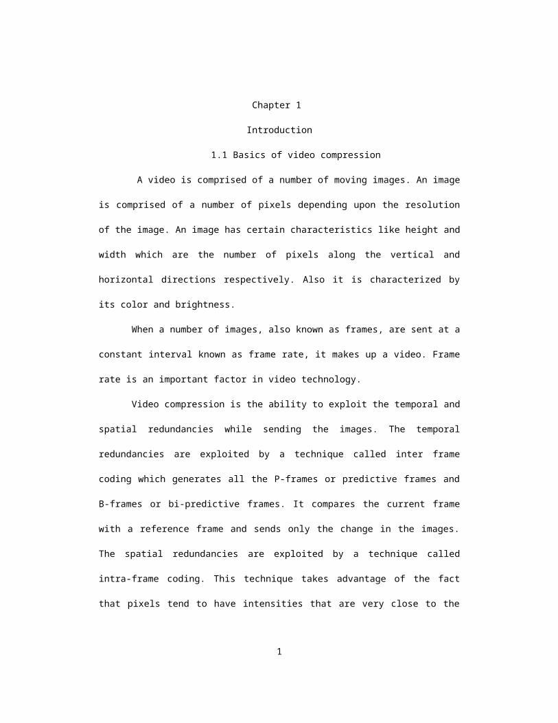
technique generates all the I-frames. The three types of frames are shown in fig 1.1 [15]

Figure 1.1 I, P and B frames [15]

1

1.2 Need for video compression:

Video compression is required in order to reduce the redundancies in video

data. Uncompressed video requires high bit rate which makes its transmission very

difficult. The higher the number of bits required, the higher is the memory space required

to store the bits. Even if the transmission and storage of such a video is taken care of,

processing power to manage such a volume of data would make the receiver hardware

very expensive. Therefore video compression is essential to overcome all these

problems.

High Efficiency Video Coding (HEVC) by JCT-VC is the latest video

compression standard which has a 50% bit rate reduction compared with the H.264

standard for the same perceptual quality [2]. HEVC has 3 profiles Main, Main intra and

Main10. These were finalized in January, 2013. In August 2013 five additional profiles

Main 12, Main 4:2:2, Main 4:4:4 10 and Mai 4:4:4 12 were released. Other range

extensions include increased emphasis on high quality coding, lossless coding and

screen content coding. Scalability extensions and 3D video extensions which enable

stereoscopic and multi-view representations and consider newer 3D capabilities such as

the depth maps and view-synthesis techniques are expected to be finalized in 2014. For

work on 3D video topics for multiple standards including 3D video extensions JCT-VC

formed a team known as JCT on 3D Video(JCT-3V) in July 2012..

1.3 Video Compression standards:

Compression of a video, while keeping the same quality, is very important since it

determines the total storage required and also affects the transmission. There have been

several video coding standards introduced by organizations like the International

Telecommunication Union - Telecommunication Standardization Sector (ITU-T), Moving

2

Picture Experts Group (MPEG) and the Joint Collaborative Team on Video Coding (JCT-

VC). Each standard is an improvement over the previous standard. Figure 1.2 shows the

evolution of the video coding standards.

Figure 1.2 Evolution of video coding standards [45]

1.4 Thesis outline:

Chapter 2 describes the high level encoding process using the HEVC standard

and various features already present in the standard like motion estimation, motion

compensation, types of predictions used, quantization and parallel processing features.

Chapter 3 describes various aspects of the inter-picture prediction of HEVC and the

motion estimation process in detail. Chapter 4 describes the analysis of the proposed

algorithm and compares it with the existing algorithm in HEVC. Chapter 6 gives the

conclusions and describes the topics that can be explored in the future.

3

Chapter 2

Overview of High Efficiency Video Coding

HEVC, the High Efficiency Video Coding standard, is the most recent joint video

project of the ITU-T VCEG and ISO/IEC MPEG standardization organizations, working

together in a partnership known as the Joint Collaborative Team on Video Coding (JCT-

VC) [1]. The HEVC standard is designed to achieve multiple goals: coding efficiency,

transport system integration and data loss resilience, as well as implementability using

parallel processing architectures [2].The main goal of the HEVC standardization effort is

to enable significantly improved compression performance relative to existing standards –

in the range of 50% bit rate reduction for equal perceptual video quality [3][4].

The block diagram of HEVC encoder is shown in figure 2.1 [2]. The

corresponding decoder block diagram is shown in figure 2.2 [5].

Figure 2.1 HEVC encoder block diagram [2]

4

Figure 2.2 HEVC decoder block diagram [5]

The video coding layer of HEVC employs the same “hybrid” approach (inter-/intra-picture

prediction and 2D transform coding) used in all video compression standards since H.261

[2]. Some differences in HEVC are coding tree units instead of macro blocks, single

entropy coding-Context Adaptive Binary Arithmetic Coding (CABAC) and features like

tiles, wave front parallel processing and dependent slices to enhance parallel processing.

The residual signal of the intra or inter prediction, which is the difference between the

original block and its prediction, is transformed by a linear spatial transform [2]. The

transform coefficients are then scaled, quantized, entropy coded, and transmitted

together with the prediction information. The residual is then added to the prediction, and

the result of that addition may then be fed into one or two loop filters to smooth out

artifacts induced by the block-wise processing and quantization. The final picture

5

representation, which is a duplicate of the output of the decoder, is stored in a decoded

picture buffer to be used for the prediction of subsequent pictures [2].

2.1 Coding tree unit:

HEVC has replaced the concept of macro blocks (MBs) with coding tree units.

The coding tree unit has a size selected by the encoder and can be larger than the

traditional macro blocks. It consists of luma coding tree blocks (CTB) and chroma CTBs.

HEVC supports a partitioning of the CTBs into smaller blocks using a tree structure and

quad tree-like signaling [2][6].

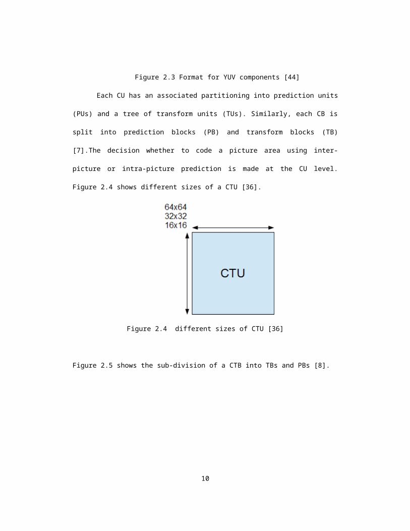
The quad tree syntax of the CTU specifies the size and positions of its luma and

chroma coding blocks (CBs). One luma CB and ordinarily two chroma CBs, together with

associated syntax, form a coding unit (CU) for 4:2:0 format.

Figure 2.3 Format for YUV components [44]

6

Each CU has an associated partitioning into prediction units (PUs) and a tree of

transform units (TUs). Similarly, each CB is split into prediction blocks (PB) and transform

blocks (TB) [7].The decision whether to code a picture area using inter-picture or intra-

picture prediction is made at the CU level. Figure 2.4 shows different sizes of a CTU [36].

Figure 2.4 different sizes of CTU [36]

Figure 2.5 shows the sub-division of a CTB into TBs and PBs [8].

7

Figure 2.5 Sub-division of a CTB into TBs and PBs [8

2.2 Encoder Features:

2.2.1:Motion vector signalling:

The HEVC standard uses a technique called advanced motion vector prediction

(AMVP) to derive several most probable candidates based on data from adjacent PBs

and the reference picture. A “merge” mode for MV coding can be also used, allowing the

inheritance of MVs from neighboring PBs [2]. Moreover, compared to H.264/MPEG-4

AVC, improved “skipped” and “direct” motion inference are also specified [2].

2.2.2 Motion compensation:

The HEVC standard uses quarter-sample precision for the MVs, and for

interpolation of fractional-sample positions it uses 7-tap (filter co-efficients: -1, 4, -10, 58,

17, -5, 1) or 8-tap filters (filter co-efficients: -1, 4, -11, 40, 40, -11, 4, 1). In H.264/MPEG-4

AVC there is 6-tap filtering (filter co-efficients: 2, -10, 40, 40, -10, 2) of half-sample

positions followed by a bi-linear interpolation of quarter-sample positions [2]. Each PB

can transmit one or two motion vectors, resulting either in uni-predictive or bi-predictive

coding, respectively [2]. As in H.264/MPEG-4 AVC, a scaling and offset operation may be

applied to the prediction signals in a manner known as weighted prediction [2].

2.2.3 Intra-picture prediction:

Intra prediction in HEVC is quite similar to H.264/AVC [7]. Samples are predicted

from reconstructed samples of neighboring blocks. The mode categories remain identical:

DC, plane, horizontal/vertical, and directional; although the nomenclature for H.264’s

plane and directional modes has changed to planar and angular modes, respectively [7].

For intra prediction, previously decoded boundary samples from adjacent PUs must be

8

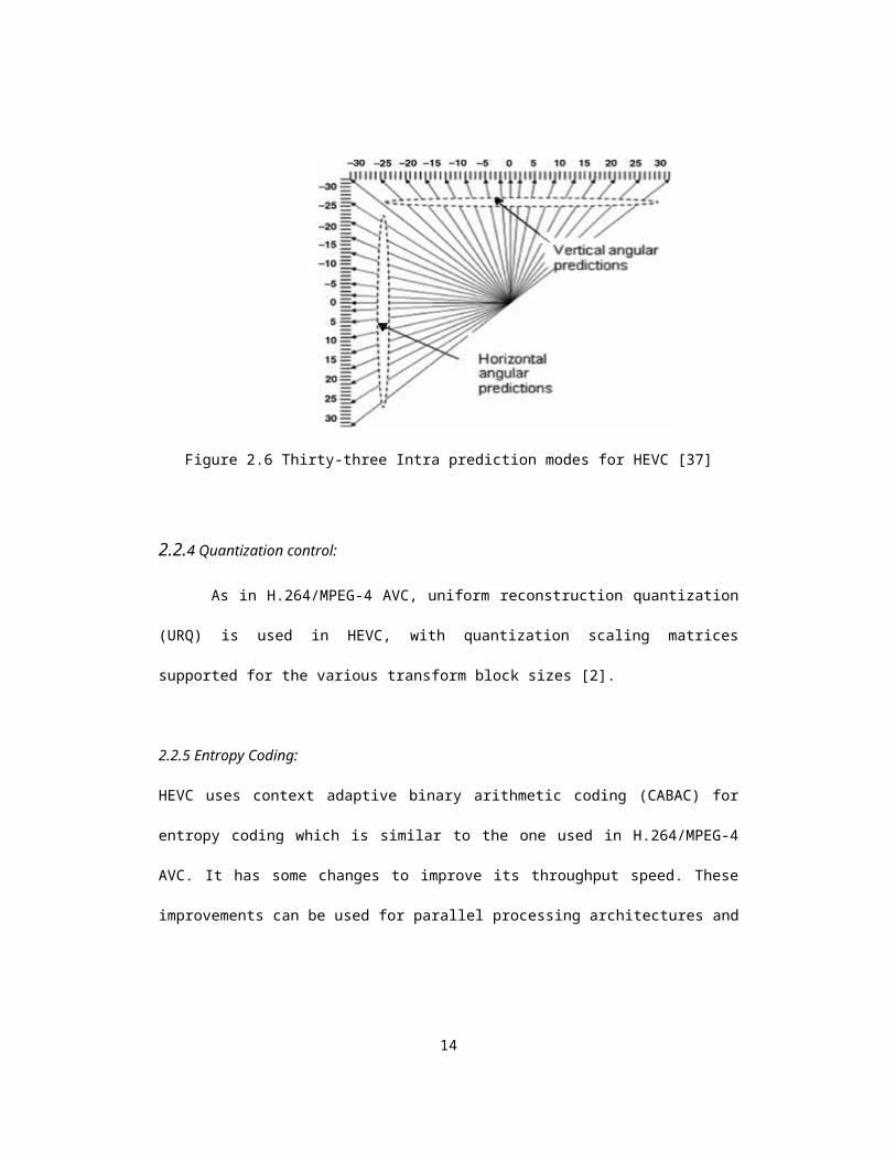
used. Directional intra prediction is applied in HEVC, which supports 17 modes for 4x4

block and 34 modes for larger blocks, inclusive of DC mode [37]. Directional intra

prediction is based on the assumption that the texture in a region is directional, which

means the pixel values will be smooth along a specific direction [37].

The increased number of directions improves the accuracy of intra prediction.

However it increases the complexity and increased overhead to signal the mode [37].

With the flexible structure of the HEVC standard, more accurate prediction, and other

coding tools, a significant improvement in coding efficiency is achieved over H.264/AVC

[37]. HEVC supports various intra coding methods referred to as Intra_Angular,

Intra_Planar and Intra_DC. In [11], an evaluation of HEVC coding efficiency compared

with H.264/AVC is provided. It shows that the average bit rate saving for random access

high efficiency (RA HE) case is 39%, while for all intra high efficiency (Intra HE) case this

bit rate saving is 25%, which is also considerable. It seems that the improvement of intra

coding efficiency is still desirable. Figure 2.6 shows different intra prediction modes for

HEVC [37].

Figure 2.6 Thirty-three Intra prediction modes for HEVC [37]

9

2.2.4 Quantization control:

As in H.264/MPEG-4 AVC, uniform reconstruction quantization (URQ) is used in

HEVC, with quantization scaling matrices supported for the various transform block sizes

[2].

2.2.5 Entropy Coding:

HEVC uses context adaptive binary arithmetic coding (CABAC) for entropy coding which

is similar to the one used in H.264/MPEG-4 AVC. It has some changes to improve its

throughput speed. These improvements can be used for parallel processing architectures

and its compression performance, and to reduce its context memory requirements.

2.2.6 In-loop deblocking filter:

The HEVC standard uses a deblocking filter in the inter-picture prediction loop as

used in H.264/MPEG-4 AVC. But design has been simplified in regard to its decision-

making and filtering processes, and is made more friendly to parallel processing [2].

2.2.7 Sample adaptive offset:

A non-linear amplitude mapping is introduced in the inter-picture prediction loop

after the deblocking filter. The goal is to better reconstruct the original signal amplitudes

by using a look up table that is described by a few additional parameters that can be

determined by histogram analysis at the encoder side [2].

2.3 High level syntax architecture:

10

The high-level syntax architecture used in the HEVC is similar to the one used in

the H.264/MPEG-4 AVC standard which includes the following features:

2.3.1 Parameter set structure:

Parameter sets contain information which can be used in the decoding of various

regions of the decoded video [2]. The concepts of sequence and picture parameter sets

from H.264/MPEG-4 AVC are augmented by a new video parameter set (VPS) structure

[2].

2.3.2 NAL unit syntax structure:

Each syntax structure is placed into a logical data packet called a network

abstraction layer (NAL) unit. Depending on the content of a two-byte NAL unit header, it

is possible to readily identify the purpose of the associated payload data [2].

2.3.3 Slices:

A slice is the part of a data structure that can be decoded independently from

other slices of the same picture, in terms of entropy coding, signal prediction, and

residual signal reconstruction [2]. It can be a picture or a region of a picture and is mainly

used for re-synchronization in case of data losses. In case of packetized transmission,

the maximum number of payload bits within a slice is typically restricted, and the number

of CTUs in the slice is often varied to minimize the packetization overhead while keeping

the size of each packet within this bound [2].

2.3.4 SEI and VUI metadata:

11

The syntax includes support for various types of metadata known as

supplemental enhancement information (SEI) and video usability information (VUI). Such

data provides information about the timing of the video pictures, the proper interpretation

of the color space used in the video signal, 3D stereoscopic frame packing information

and other “display hint” information [2].

2.4 Parallel processing features:

HEVC has four new features to enhance parallel processing capability or modify

the structuring of slice data for packetization purposes.

2.4.1 Tiles:

HEVC has an option of partitioning its picture into rectangular independently

decodable regions called as tiles. Its main purpose is for parallel processing. Tiles can

also be used for random access to local regions in video pictures. Tiles provide

parallelism at a more coarse level (picture/sub-picture) of granularity, and no

sophisticated synchronization of threads is necessary for their use.

2.4.2 Wavefront parallel processing (WPP):

This is a new feature in HEVC which when enabled allows a slice to be divided

into rows of CTUs. The processing of each row can be started only after certain decisions

in the previous row have been made. WPP provides parallelism within slices [2]. Figure

2.7 shows how WPP works [7]

12

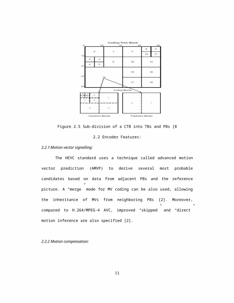
Figure 2.7 CTBs processed in parallel using WPP [7]

2.4.3 Dependent slices:

Dependent slices allow data associated with a particular wave front point entry or

tile to be carried in a separate NAL unit. It also allows fragmented packetization of the

data with lower latency than if it were all coded in one slice [2].

2.5 Summary:

Chapter 2 describes the overview of the HEVC standard, encoder features, high

level syntax architecture and parallel processing capabilities. Chapter 3 will describe the

details regarding different blocks of inter picture prediction and motion estimation.

13

Chapter 3

Inter Picture Prediction

Inter picture prediction in the HEVC standard is divided into prediction block

partitioning, fractional sample interpolation and motion vector prediction for merge and

non-merge modes. The HEVC standard supports more PB partition shapes for inter-

coded CBs. The samples of the PB for an inter-coded CB are obtained from those of a

corresponding block region in the reference picture identified by a reference picture

index, which is at a position displaced by the horizontal and vertical components of the

motion vector.

The HEVC standard only allows a much lower number of candidates to be

used in the motion vector prediction process for the non-merge case, since the encoder

can send a coded difference to change the motion vector. Further, the encoder needs to

perform motion estimation, which is one of the most computationally expensive

operations in the encoder, and complexity is reduced by allowing less number of

candidates [2]. When the reference index of the neighboring PU is not equal to that of the

current PU, a scaled version of the motion vector is used [2]. The neighboring motion

vector is scaled according to the temporal distances between the current picture and the

reference pictures indicated by the reference indices of the neighboring PU and the

current PU, respectively [2]. When two spatial candidates have the same motion vector

components, one redundant spatial candidate is excluded [2].

14

Figure 3.1 illustrates the block based motion estimation process [5].

Figure 3.1 block based motion estimation process [5].

Figure 3.2 HEVC motion estimation flow

15

In multi-view video coding, both temporal and interview redundancies can be exploited by

using standard block based motion estimation (BBME) [38]. Due to its simplicity and

efficiency [38], the BBME [39] has been adopted in several international video coding

standards such as MPEG-x, H.26x and VC-1 [40][41]. In the BBME, the current frame is

divided into NxN pixel size macroblocks (MBs) and for each MB a certain area of the

reference frame is searched to minimize a block difference measure (BDM), which is

usually a sum of absolute differences (SAD) between the current MB and the reference

MB [21]. The displacement within the search area (SA) which gives the minimum BDM

value is called a motion vector [21]. With the development of video coding standards, the

basic BBME scheme was extended by several additional techniques such as sub-pixel,

variable block size, and multiple reference frame motion estimation [39]. Figure 3.3

shows multiple frame reference frame motion estimation [25].

Figure 3.3 Multiple frame reference frame motion estimation [25]

16

Figure 3.4 shows variable block sizes in motion estimation [33].

Figure 3.4 Variable block sizes in motion estimation HEVC [33]

3.1 Prediction block partitioning

Compared with intra coded CBs, HEVC provides a greater number of partition

shapes for inter coded CBs [2]. The partition mode PART_2Nx2N means there is no

partition of the CB whereas PART_Nx2N and PART_2NxN means the CB is split in equal

size vertically and horizontally respectively. PART_NxN means that the CB is split equally

into four parts but this mode is only supported when the size of the CB is equal to the

smallest allowed size [2]. The HEVC standard also supports asymmetric motion partitions

PART_2N×nU, PART_2N×nD, PART_nL×2N and PART_nR×2N. Figure 3.5 shows the

partition sizes

17

Figure 3.5 Inter picture partitions in HEVC [43]

3.2 Fractional sample Interpolation

The samples of the PB for an inter-coded CB are obtained from those of a

corresponding block region in the reference picture identified by a reference picture

index, which is at a position displaced by the horizontal and vertical components of the

motion vector [2]. Fractional sample interpolation is used to generate the prediction

samples for non-integer sampling positions when the motion vector does not have an

integer value.

HEVC uses an 8-tap filter (weights: -1, 4, -11, 40, 40, -11, 4, 1) for the half-

sample positions for fractional sample interpolation of luma samples and a 7-tap filter

(weights: -1, 4, -10, 58, 17, -5, 1) for quarter sample positions. Figure 3.6 shows the

fractional sample interpolation used in HEVC.

18

Figure 3.6 Integer and fractional sample positions for luma interpolation [2]

Unlike H.264/AVC which uses a two-stage interpolation process by first

generating the values of one or two neighboring samples at half-sample positions using

6-tap filtering, rounding the intermediate results, and then averaging two values at integer

or half-sample positions which is as follows:

a0, j=( ∑i=−3 .. . 3

A i , j qfilter [ i ]) >> (B−8 )b0, j=( ∑

i=−3 .. . 4Ai , jhfilter [i ] ) >> (B−8 )

c0 , j=( ∑i=−2. .. 4

A i , j qfilter [1−i ]) >> (B−8 )

d0,0=( ∑j=−3 . .. 3

A0 , jqfilter [ j ] ) >> (B−8 )

19

h0,0=( ∑j=−3. . . 4

A0 , jhfilter [ j ]) >> (B−8 )

n0,0=( ∑j=−2. .. 4

A0 , jqfilter [1− j ]) >> (B−8 )

The constant B>=8 is the bit-depth of the reference samples(B=8 for most

applications) [2]. In these formulas, ‘>>’ denote an arithmetic right shift operation.

The samples labeled e0, 0, f0, 0, g0, 0, i0, 0, j0, 0, k0, 0 , q0,0 , p0,0 and r0 , 0 can be derived

by applying the corresponding filters to samples located at vertically adjacent a0, j, b0, j and

c0, j positions as follows:

e0,0=( ∑v=−3. . . 3

a0 , vqfilter [v ]) >> 6f 0,0=( ∑

v=−3. . .3b0, vqfilter [v ]) >> 6

g0,0=( ∑v=−3 .. . 3

c0, vqfilter [v ]) >> 6i0,0=( ∑

v=−3. . . 4a0 , vhfilter [v ] ) >> 6

j0,0=( ∑v=−3 . .. 4

b0 , vhfilter [v ]) >> 6k 0,0=( ∑

v=−3. .. 4c0, vhfilter [v ]) >> 6

p0,0=( ∑v=−2 .. . 4

a0, vqfilter [1−v ]) >> 6q0,0=( ∑

v=−2. . . 4b0 , vqfilter [1−v ] ) >> 6

r0,0=( ∑v=−2 .. . 4

c0 , vqfilter [1−v ]) >> 6

20

The HEVC standard instead uses a single, consistent, separable interpolation

process to generate all fractional positions without intermediate rounding operations. It

improves precision and simplifies the architecture of the fractional sample interpolation.

The fractional sample interpolation process for the chroma components is similar to the

one for the luma component. But the number of filter taps is 4 and the fractional accuracy

is 1/8 for the usual 4:2:0 chroma format case (fig. 2.3).

3.3 Merge mode in HEVC

In inter-prediction, motion information basically consists of horizontal and vertical

motion vector displacement values, and one or two reference picture indices in the case

of prediction regions in B slices, an identification of which reference picture list is

associated with each index [2]. A merge mode is used in HEVC to get this information

from spatially or temporally neighboring blocks. Since it uses a merged region sharing all

motion information, it is called as merge mode in HEVC. The merge mode is conceptually

similar to the direct and skip modes in H.264/MPEG-4 AVC; however, there are two

important differences. First, the HEVC standard transmits index information to select one

out of several available candidates, in a manner sometimes referred to as a motion

vector “competition” scheme. The HEVC standard also explicitly identifies the reference

picture list and reference picture index; whereas the direct mode assumes that these

have some pre-defined values [2].

Merge mode includes a set of possible candidates consisting of spatial

neighboring candidates, a temporal candidate and generated candidates. Figure 3.7

shows the position of spatial candidates and for each candidate, the availability is

checked in the order a1, b1, b0, a0, b2 [2].

21

Figure 3.7 Positions of spatial candidates [2]

There are two kinds of redundancies which are removed after the validation of

the spatial candidates. The first is if the candidate position for the current PU refers to

the first PU within the same CU, it means that the same merge could be achieved by a

CU without splitting it into prediction partitions. Hence it is removed. The second is when

the candidates have the same motion information.

For the temporal candidate, the right bottom position just outside of the

collocated PU of the reference picture is used if it is available. Otherwise, the center

position is used instead [2]. The HEVC standard provides more flexibility than H.264 by

transmitting the index of the reference picture list used for the collocated reference

picture. Since temporal candidates use more memory, the granularity for storing the

temporal motion candidates is restricted to a resolution of 16x16 luma grid, even when

smaller PB structures are used at the corresponding location in the reference picture.

The total number of merge candidates is provided in the slice header. If it goes

above the specified number, only the first candidates equal to the number specified are

considered. If it is less than the specified number, additional candidates are generated to

match the specified number.

22

3.4 Motion vector prediction

If the merge mode is not used, then a motion vector predictor is used to

differentially code the motion vector. This mode is called the non-merge mode. Like

merge mode, it also consists of multiple predictor candidates. The difference between the

actual motion vector and the predictor is calculated and is sent to the decoder along with

the index of the predicted motion vector candidate. Only two of the five spatial candidates

is used in the non-merge mode according to the availability. So if the merge and non-

merge modes are compared, HEVC allows a much lower number of candidates for the

non-merge mode. This is because if the number of candidates is low, the encoder can

send the coded difference and hence can change the motion vector. The reason for

sending a fewer number of candidates is that the encoder needs to perform motion

estimation which is a computationally complex process and the complexity is reduced if

the number of candidates is low. When the reference index of the neighboring PU is not

equal to that of the current PU, a scaled version of the motion vector is used [2]. The

neighboring motion vector is scaled according to the temporal distances between the

current picture and the reference pictures indicated by the reference indices of the

neighboring PU and the current PU, respectively. When two spatial candidates have the

same motion vector components, one redundant spatial candidate is excluded. The

temporal motion vector prediction candidate is only included when the number of motion

vector candidates is not equal to two and the use of temporal motion vector prediction is

not disabled.

23

3.5 Proposed method

The existing algorithm of the motion estimation uses the block given by the predicted

motion vector as the starting point to code the actual motion vectors. Once the starting

point is decided, a search algorithm such as square search, diamond search or full

search are used to calculate the sum of absolute differences (SAD) between the

neighboring blocks in the reference frame and the current block which is to be encoded.

Each time a block is checked and SAD is calculated it is compared with the best SAD. If

the current SAD is less than the best SAD, it is declared as the best SAD. The total time

taken by the search algorithm constitutes longest part of the motion estimation process.

However, it is observed that if the SAD of the block given by the predicted motion vector

value is precise, then the search pattern can be terminated if the SAD of any search point

goes below a threshold [21]. The threshold can be calculated using the sum of absolute

differences of the predicted motion vector and if a search point meets this requirement it

can be declared as the winning point. The current step of the search process can be

ended and hence the time taken for unnecessary calculations of the remaining search

points in that step can be reduced. As the number of steps increase and the number of

search points increase, the early termination can produce a lot of time saving.

3.6 Summary

Chapter 3 describes the motion estimation process and the existing search

algorithm along with a method to optimize and reduce the encoding time. Chapter 4 gives

the results and graphs of the comparison of the existing algorithm and the proposed

algorithm by testing it on various test sequences for different quantization parameters.

24

Chapter 4

4.1 Test conditions

To test the performance of the proposed motion merge encoding technique the

HEVC reference software HM 13.0 [38] was used. The encoder random access profile

was used for testing purposes with a Group of Pictures (GOP) of length 8. The ‘encoder

random access profile’ encodes the first frame as an intra-frame (I frame) and the

following 7 frames are inter frames with bi-directional prediction (B-frames) .It follows a

non-sequential approach towards selecting the next frame for encoding as shown in

Figure 4.1. POC is the Picture Order Count.

4.1 GOP structure of encoder random access profile

The proposed algorithm was tested for 5 different test sequences [40] with

resolutions going from WQVGA (416 x 240) up to high definition (1920 x 1080). Each test

sequence was then run with 4 different quantization parameters of 22, 27, 32 and 37

which are commonly used for comparison/evaluation of various techniques. The list of

test sequences is given in the table 4.1:

25

No Sequence Resolution Type No of frames

1 Race Horses 416x240 WQVGA 30

2 BQ Mall 832x480 WVGA 30

3 BasketBallDrillText 832x480 WVGA 30

4 Kristen and Sara 1280x1080 SD 30

5 Parkscene 1920x1080 HD 30

Table 4.1 List of test sequences [40] (all sequences at 30 fps)

4.2 Reduction in encoding time:

The proposed algorithm has reduced the encoding time of the test sequences by

about 5 to 17% as compared to the existing algorithm in the HEVC reference software

HM 13.0 [38] for different quantization parameters. The PSNR change is less than 1 dB

compared to the existing algorithm in the HEVC reference software HM13.0. Figures 4.2

through 4.6 show comparison graphs of the time taken by the existing algorithm against

the proposed algorithm for 4 quantization parameters 22, 27, 32 and 37. The total

number of frames considered for all the test sequences is 30.

26

22 27 32 370

200

400

600

800

1000

1200

1400

16001394.02

1110.753 903.756

753.122

1323.65

1022.239812.419

656.715 originalproposed

Race Horses-WQVGA-30 frames

Qp

Enco

ding

tim

e (s

ec)

Figure 4.2 Encoding time versus QP for Race Horses (416x240)

22 27 32 370

500

1000

1500

2000

2500

3000

3500

40003344.474

2759.522383.185

2133.866

3049.212

2467.3162075.006

1839.711 originalproposed

BQ Mall-WVGA-30 frames

Qp

Enco

ding

tim

e (s

ec)

Figure 4.3 Encoding time versus QP for BQ Mall (832x480)

27

22 27 32 370

500

1000

1500

2000

2500

3000

3500

4000 3795.112

3114.593 2611.741

2282.861

3513.106

2795.1512268.961

1961.797originalproposed

BasketBallDrillText-WVGA-30 frames

Qp

Enco

ding

tim

e (s

ec)

Figure 4.4 Encoding time versus for BasketBallDrillText (832x480)

22 27 32 370

1000

2000

3000

4000

5000

60005230.557

4560.6324308.201

4031.441

4544.291

3899.955 3562.4713374.153

originalproposed

Kristen and Sara-SD-30 frames

Qp

Enco

ding

tim

e (s

ec)

Figure 4.5 Encoding time versus QP for Kristen and Sara (1280x720)

28

22 27 32 370

2000

4000

6000

8000

10000

12000

14000

16000

18000 16588.689

13091.34611353.34

10315.036

15210.024

11733.109

9648.017 8583.977originalproposed

Park Scene - HD - 30 frames

QP

Enco

ding

tim

e(se

c)

Figure 4.6 Encoding time versus QP for Park Scene (1920x1080)

29

Figures 4.7 through 4.11 show the comparison graphs of the bit-rate increase

between the existing algorithm and the proposed algorithm.

22 27 32 370

200

400

600

800

1000

1200

1400

1600

18001443.872

724.936

362.28

185.016

1643.664

786.544

379.408

188.528

originalproposed

Bit-r

ate

incr

ease

(Kbp

s)Race Horses -WQVGA-30 frames

QP

Figure 4.7 Bit-rate versus QP for Race Horses (416x240)

22 27 32 370

500

1000

1500

2000

25001935.968

942.528

474.12256.664

2135.416

1004.936

490.208

261.2

originalproposed

Bit-r

ate

incr

ease

(Kbp

s)

BQ Mall -WVGA-30 frames

QP

Figure 4.8 Bit-rate versus QP for BQ Mall (832x480)

30

22 27 32 370

500

1000

1500

2000

2500

3000

2222.256

1070.696

553.344296.952

2400.064

1163.656

584.696

309.496

Originalproposed

Bit-r

ate

incr

ease

(Kbp

s)

BasketBallDrillText -WVGA-30 frames

QP

Figure 4.9 Bit-rate versus QP for BasketBallDrillText (832x480)

22 27 32 370

200

400

600

800

1000

1200

14001171.816

507.784

266.296148.184

1218.336

522.408

269.648

150.36

Originalproposed

Bit-r

ate

incr

ease

(Kbp

s)

Kristen and Sara -SD-30 frames

QP

Figure 4.10 Bit-rate versus QP for Kristen and Sara (1280x720)

31

22 27 32 370

2000

4000

6000

8000

10000

120009610.968

4071.8

1834.792834.32

10480.408

4306.96

1885.136

843.936

Originalproposed

Bit-r

ate

incr

ease

(Kbp

s)

Park Scene -HD-30 frames

QP

Figure 4.11 Bit-rate versus QP for Kristen and Sara (1920x1080)

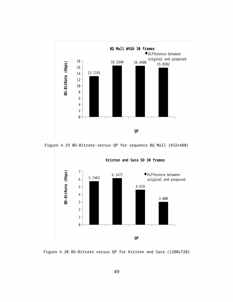
4.3 BD-PSNR and BD-Bitrate

Bjøntegaard Delta PSNR (BD-PSNR) was proposed to objectively evaluate the

coding efficiency of video codecs [39]. BD-PSNR is able to provide a good evaluation of

the R-D performance based on the Rate-Distortion(R-D) curve fitting but with one critical

drawback [39]. It does not consider the complexity of the coding while evaluating, yet it

indicates the quality of the video [38][40]. It suggests that to improve the video codec, the

BD-PSNR value should increase and the BD-Bitrate should decrease. The following

figures are a plot of BD-PSNR and BD-Bitrate versus the quantization parameters for the

test sequences.

32

-3

-2.5

-2

-1.5

-1

-0.5

0

-2.4183

-1.7854

-1.1622

-0.63

Difference between original and proposed

QP

BD-P

SNR

(dB)

Race Horses WQVGA 30 frames

Figure 4.12 BD-PSNR versus QP for Race Horses (416x240)

-2-1.8-1.6-1.4-1.2

-1-0.8-0.6-0.4-0.2

0

-1.763

-1.2547

-0.7477

-0.4354

Difference between original and proposed

QP

BD-P

SNR

(dB)

BasketBallDrillText WVGA 30 frames

Figure 4.13 BD-PSNR versus QP for BasketBallDrillText (832x480)

33

-1.6

-1.4

-1.2

-1

-0.8

-0.6

-0.4

-0.2

0

-1.2644

-1.4409

-1.0617 -1.0617

Difference between original and proposed

QP

BD-P

SNR

(dB)

BQ Mall WVGA 30 frames

Figure 4.14 BD-PSNR versus QP for BQ Mall (832x480)

22 27 32 37

-0.8

-0.7

-0.6

-0.5

-0.4

-0.3

-0.2

-0.1

0

-0.7473

-0.6338

-0.3395 -0.3574

Difference between original and proposed

QP

BD-P

SNR

(dB)

Kristen and Sara SD 30 frames

Figure 4.15 BD-PSNR versus QP for Kristen and Sara (1280x720)

34

-1.4

-1.2

-1

-0.8

-0.6

-0.4

-0.2

0

-1.3003

-0.9629

-0.5494

-0.2679

Difference between original and proposed

QP

BD-P

SNR

(dB)

Park Scene HD 30 frames

Figure 4.16 BD-PSNR versus QP for Park scene (1920x1080)

05

101520253035404550

39.467943.9024

33.1171

21.4365

Difference between original and proposed

QP

BD-B

itRat

e (K

bps)

Race Horses WQVGA 30 frames

Figure 4.17 BD-Bitrate versus QP for Race Horses (416x240)

35

0

5

10

15

20

2522.5899

19.1387

14.124

8.9455

Difference between original and proposed

QP

BD-B

itRat

e (K

bps)

BasketBallDrillText WVGA 30 frames

Figure 4.18 BD-Bitrate versus QP for BasketBallDrillText (832x480)

0

2

4

6

8

10

12

14

16

18

13.1191

16.5348 16.4486 15.8582

Difference between original and proposed

QP

BD-B

itRat

e (Kb

ps)

BQ Mall WVGA 30 frames

Figure 4.19 BD-Bitrate versus QP for sequence BQ Mall (832x480)

36

0

1

2

3

4

5

6

7

5.74836.1477

4.618

3.008

Difference between original and proposed

QP

BD-B

itRat

e (K

bps)

Kristen and Sara SD 30 frames

Figure 4.20 BD-Bitrate versus QP for Kristen and Sara (1280x720)

0

5

10

15

20

25 23.160321.5803

15.0043

7.8196

Difference between original and proposed

QP

BD-B

itRat

e (K

bps)

Park Scene HD 30 frames

Figure 4.21 BD-Bitrate versus QP for Park Scene (1920x1080)

37

4.4 Rate Distortion Plot

The proposed algorithm has a negligible reduction in PSNR with a slight increase

in the bit-rate for low resolution sequences. Figures 4.16 through 4.20 show the graphs of

the PSNR vs bitrate for the test sequences.

100 300 500 700 900 1100 1300 1500 1700 19002527293133353739414345

Original Proposed

BitRate(Kbps)

Race Horses-WQVGA-30 frames

PSNR

(dB)

Figure 4.22 PSNR versus Bitrate for sequence Race Horses (416x240)

38

100 300 500 700 900 1100 1300 1500 1700 1900 2100 23002527293133353739414345

Original Proposed

BitRate(Kbps)

BasketBallDrillText-WVGA-30 framesPS

NR (d

B)

Figure 4.23 PSNR versus Bitrate for sequence BasketBallDrillText (832x480)

100 600 1100 1600 2100 260025

27

29

31

33

35

37

39

41

Original Proposed

BitRate(Kbps)

BQ Mall-WVGA-30 frames

PSNR

(dB)

Figure 4.24 PSNR versus Bitrate for sequence BQ Mall (832x480)

39

100 200 300 400 500 600 700 800 900 1000 1100 1200 130032

34

36

38

40

42

44

Original Proposed

BitRate(Kbps)

Kristen and Sara-SD-30 framesPS

NR (d

B)

Figure 4.25 PSNR versus Bitrate for sequence Kristen and Sara (1280x720)

100 1600 3100 4600 6100 7600 9100 10600 1210025

27

29

31

33

35

37

39

41

Original Proposed

BitRate(Kbps)

Park Scene-HD-30 frames

PSNR

(dB)

Figure 4.26 PSNR versus Bitrate for sequence Park Scene (1920x1080)

40

4.5 Summary

In this chapter, results and graphs for different test sequences and quantization

parameters have been plotted which compare the original HEVC algorithm to the one

proposed. Different factors like BD-PSNR, BD-bit-rate and encoding time have been

considered while getting the results. Chapter 5 gives the conclusions and describes the

topics that can be explored in the future.

41

Chapter 5

5.1 Conclusions and Future work

An early termination of the search algorithm is proposed to reduce the total time

taken by the motion estimation process in the HEVC encoder. The search algorithm

which is used to calculate motion vectors takes most of the time. Any reduction of time in

this process, results in reduction of the overall encoding time. The proposed method uses

the predicted motion vectors to calculate a threshold and terminate the search process if

the SAD value falls below this threshold. Comparison of the proposed algorithm with the

existing algorithm shows that the encoding time has been reduced by 5% to 17% with a

negligible PSNR loss of less than 1 dB. The results also show an increase in the bitrate

by 1% to 13%, however it increases by 13% only for 1 case out of 20 (5 test sequences

x 4 quantization parameters). Otherwise, the bit-rate increase is typically in the range of

2% to 7%. The BD-PSNR decreased only by 0.3 dB to 2.4 dB and BD-Bitrate increased

only by 7 to 43 Kbps.

5.2 Future work

The proposed early termination algorithm can be used with different search

patterns such as hexagon or octagon patterns [41] or adaptive patterns. The HEVC

standard also supports parallel processing which if used can result in a lot of reduction of

the time taken. There are many blocks in the HEVC standard (fig.2.1) which can be

parallelized like getting motion information of different PUs, CUs or search points. The

use of GPUs can considerably increase the processing speed and reduce the encoding

time due to the availability of a greater number of threads. GPU implementation can be

42

done using CUDA [7][8] or OpenGL. However, the dependency needs to be considered

while using the parallel processing technique.

Complexity can also be reduced using hardware implementations at various

encoder levels and optimizing parallel processing features. It can be implemented in a

FPGA for evaluation purposes and the performance can be compared with the existing

one.

43

Appendix A

Test Sequences[40]

44

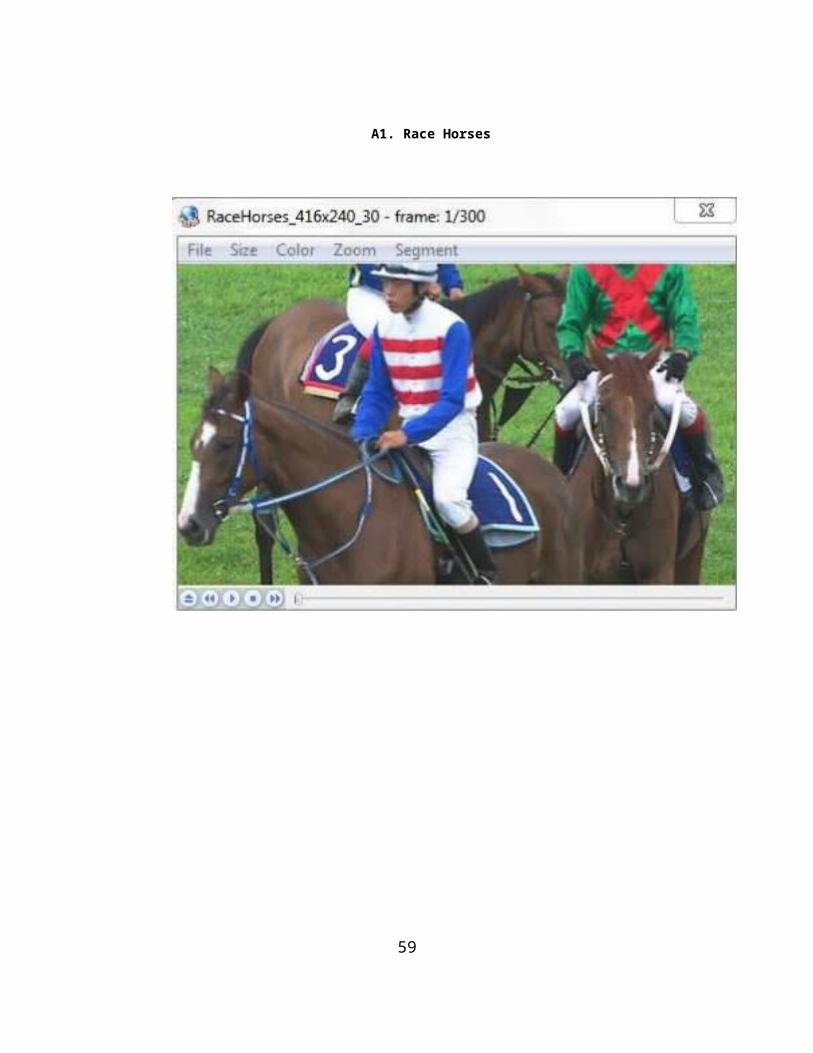
A1. Race Horses

45

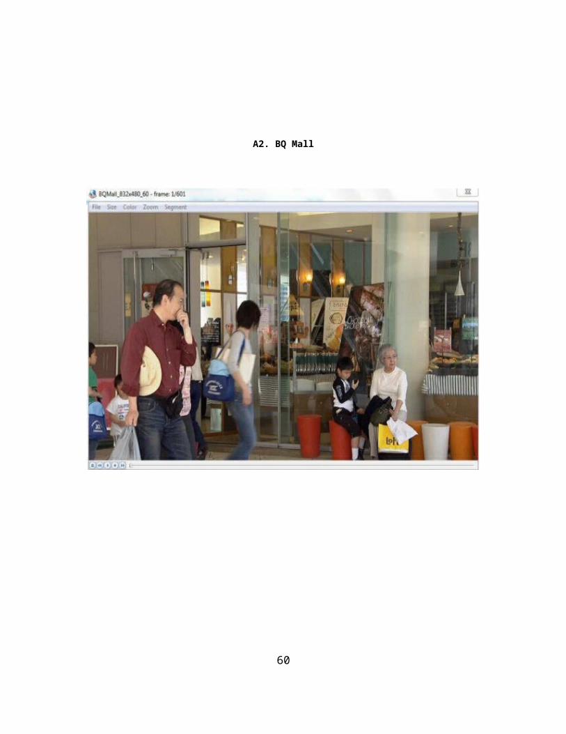
A2. BQ Mall

A3. BasketBallDrillText

46

47

A4. Kristen and Sara

48

A.5 Park Scene

49

Appendix B

Test Conditions

50

The code revision used for this work is HM 13 [38].The work was done using intel core

i-7 processor with Microsoft windows 7 64 bit version running with 8GB RAM and 2.2 GHz

speed.

51

Appendix C

BD-PSNR and BD-Bitrate [52][53]

52

ITU - Telecommunications Standardization SectorSTUDY GROUP 16 Question 6Video Coding Experts Group (VCEG)_________________Thirteenth Meeting: Austin, Texas, USA, 2-4 April, 2001

Document VCEG-M33Filename: VCEG-M33.docGenerated: 26 March ’01

Question: Q.6/SG16 (VCEG)

Source: Gisle BjontegaardTelenor Satellite ServicesP.O.Box 6914 St.Olavs plassN-0130 Oslo, Norway

Tel:Fax:Email:

+47 23 13 83 81+47 22 77 79 80gisle.bjontegaard@telenor.com

Title: Calculation of average PSNR differences between RD-curves

Purpose: Proposal

_____________________________

Introduction

VCEG-L38 defines "Recommended Simulation Conditions for H.26L".

One of the outcomes is supposed to be RD-plots where PSNR and bitrate

differences between two simulation conditions may be read. The present

document describes a method for calculating the average difference between two

such curves. The basic elements are:

Fit a curve through 4 data points (PSNR/bitrate are assumed to be

obtained for QP = 16,20,24,28)

Based on this, find an expression for the integral of the curve

The average difference is the difference between the integrals divided by

the integration interval

53

IPR

“The contributor(s) are not aware of any issued, pending, or planned

patents associated with the technical content of this proposal.”

Fitting a curve

A good interpolation curve through 4 data points of a "normal" RD-curve

(see figure 1) can be obtained by:

SNR = (a + b*bit + c*bit2)/(bit + d)

where a,b,c,d are determined such that the curve passes through all 4 data

points.

This type of curve is well suited to make interpolation in "normal" luma curves.

However, the division may cause problems. For certain data (Jani pointed out some

typical chroma data) the obtained function may have a singular point in the range of

integration - and it fails.

Use of logarithmic scale of bitrate

When we look at figure 1, the difference between the curves is dominated by the

high bitrates.

The range (1500-2000) gets 4 times the weight of the range (375-500) even if

they both represent a bitrate variation of 33%

Hence it was considered to be more appropriate to do the integration based on

logarithmic scale of bitrate. Figure 2 shows a plot where "Logarithmic x-axes" is used in

the graph function of Excel. However, this function has no flexibility and only allows

factors of 10 as units.

54

In figure 3 I first took the logarithm of bitrates and the plot has units of "dB" along

both axes. The factor between two vertical gridlines in the plot is: 100.05 = 1.122 (or

12.2%). Could this be an alternative way of presenting RD-plots?

Interpolation with logarithmic bitrate scale

With logarithmic bitrate scale the interpolation can also be made more straight

forward with a third order polynomial of the form:

SNR = a + b*bit + c*bit2 + d*bit3

This result in good fit and there is no problems with singular points. This is

therefore the function I have used for the calculations in VCEG-M34. However, for

integration of luma curves the results are practically the same as with the first integration

method which was used for the software distributed by Michael regarding the complexity

experiment.

In the same way we can do the interpolation to find Bit as a function of SNR:

SNR = a + b*SNR + c*SNR2 + d*SNR3

In this way we can find both:

Average PSNR difference in dB over the whole range of bitrates

Average bitrate difference in % over the whole range of PSNR

On request from Michael average differences are found over the whole

simulation range (see integration limits in figure 3) as well as in the middle section -

called mid range.

As a result VCEG-M34 shows 4 separate data tables.

Conclusions

It is proposed to include this method of finding numerical averages

between RD-curves as part of the presentation of results. This is a more compact

55

and in some sense more accurate way to present the data and comes in addition

to the RD-plots.

The distinction between "total range" and "mid range" does not seem to

add much and it is therefore proposed to use "total range" only.

From the data it is seen that relation between SNR and bitrate is well

represented by 0.5 dB = 10% or 0.05 dB = 1% It is therefore proposed to

calculate either change in bitrate or change in PSNR.

Should it be considered to present RD-plots as indicated in figure 3?

56

Figure 1

57

"Normal" RD-plot

25

26

27

28

29

30

31

32

33

34

35

0 500 1000 1500 2000 2500Bitrate

PSNR

(dB)

Plot2Plot1

Figure 2

58

Log X-axes

25

26

27

28

29

30

31

32

33

34

35

100 1000 10000Bitrate

PSNR

(dB)

Plot2Plot1

Figure 3

Here is a document about BD-PSNR which has been referenced by many Video Engineers. You can download it at http://wftp3.itu.int/av-arch/video-site/

The matlab code for computing BD-Bitrate and BD-PSNR is found in this link:http://www.mathworks.com/matlabcentral/fileexchange/27798-bjontegaardmetric/content/bjontegaard.m

function avg_diff = bjontegaard(R1,PSNR1,R2,PSNR2,mode)

%BJONTEGAARD Bjontegaard metric calculation% Bjontegaard's metric allows to compute the average gain in PSNR or the% average per cent saving in bitrate between two rate-distortion% curves [1].% Differently from the avsnr software package or VCEG Excel [2] plugin this% tool enables Bjontegaard's metric computation also with more than 4 RD% points.

59

Log/Log plot

25

26

27

28

29

30

31

32

33

34

35

25 26 27 28 29 30 31 32 33 3410xlog(bitrate)

PSNR

(dB)

Plot2Plot1Lim2Lim1Lim4Lim3

%% R1,PSNR1 - RD points for curve 1% R2,PSNR2 - RD points for curve 2% mode - % 'dsnr' - average PSNR difference% 'rate' - percentage of bitrate saving between data set 1 and% data set 2%% avg_diff - the calculated Bjontegaard metric ('dsnr' or 'rate')% % (c) 2010 Giuseppe Valenzise%% References:%% [1] G. Bjontegaard, Calculation of average PSNR differences between% RD-curves (VCEG-M33)% [2] S. Pateux, J. Jung, An excel add-in for computing Bjontegaard metric and% its evolution

% convert rates in logarithmic unitslR1 = log(R1);lR2 = log(R2);

switch lower(mode) case 'dsnr' % PSNR method p1 = polyfit(lR1,PSNR1,3); p2 = polyfit(lR2,PSNR2,3);

% integration interval min_int = min([lR1; lR2]); max_int = max([lR1; lR2]);

% find integral p_int1 = polyint(p1); p_int2 = polyint(p2);

int1 = polyval(p_int1, max_int) - polyval(p_int1, min_int); int2 = polyval(p_int2, max_int) - polyval(p_int2, min_int);

% find avg diff

60

avg_diff = (int2-int1)/(max_int-min_int);

case 'rate' % rate method p1 = polyfit(PSNR1,lR1,3); p2 = polyfit(PSNR2,lR2,3);

% integration interval min_int = min([PSNR1; PSNR2]); max_int = max([PSNR1; PSNR2]);

% find integral p_int1 = polyint(p1); p_int2 = polyint(p2);

int1 = polyval(p_int1, max_int) - polyval(p_int1, min_int); int2 = polyval(p_int2, max_int) - polyval(p_int2, min_int);

% find avg diff avg_exp_diff = (int2-int1)/(max_int-min_int); avg_diff = (exp(avg_exp_diff)-1)*100;end

61

Appendix D

Acronyms

62

AVC - Advanced Video Coding

AMVP – Advanced Motion Vector Prediction

BBME- Block Based Motion estimation

BD - Bjontegaard Delta

BDM-

CABAC – Context Adaptive Binary Arithmetic Coding

CB – Coding Block

CBF – Coding Block Flag

CFM – CBF Fast Mode

CTU – Coding Tree Unit

CTB – Coding Tree Block

CU – Coding Unit

CUDA- Compute unified device architecture

DCT – Discrete Cosine Transform

DST – Discrete Sine Transform

GOP-Group of pictures

FPGA- Field programmable gate arrays

HDTV - High Definition Tele Vision

HDR - High Dynamic Range

HDRI - High Dynamic Range Imaging

HEVC – High Efficiency Video Coding

HM – HEVC Test Model

HVS – Human Visual System

ISO – International Standards Organization

ITU – International Telecommunication Union

63

JCT-VC - Joint Collaborative Team on Video Coding

JVT- Joint video team

KTA- Key technical areas

MB – Macroblock

MC – Motion Compensation14

ME – Motion Estimation

MPEG – Moving Picture Experts Group

NAL – Network Abstraction Layer

PB – Prediction Block

POC-Picture order count

PSNR – Peak Signal to Noise Ratio

PU – Prediction Unit

QP – Quantization Parameter

RDOQ – Rate Distortion Optimization Quantization

RGB – Red Green Blue

RMD – Rough Mode Decision

SAD-Sum of absolute differences

SATD – Sum of Absolute Transform Differences

SD – Standard Definition

SSIM – Structural Similarity

TB – Transform Block

TU – Transform Unit

URQ – Uniform Reconstruction Quantization

VCEG – Video Coding Experts Group

VPS – Video Parameter Set

64

WQVGA – Wide Quarter Video Graphics Array

WVGA – Wide Video Graphics Array

65

Appendix E

Code for the proposed algorithm

The following section of the HEVC code has been modified to implement the proposed

algorithm

66

__inline Void TEncSearch::xTZ8PointDiamondSearch( TComPattern* pcPatternKey, IntTZSearchStruct& rcStruct, TComMv* pcMvSrchRngLT, TComMv* pcMvSrchRngRB, const Int iStartX, const Int iStartY, const Int iDist ){ Int iSrchRngHorLeft = pcMvSrchRngLT->getHor(); Int iSrchRngHorRight = pcMvSrchRngRB->getHor(); Int iSrchRngVerTop = pcMvSrchRngLT->getVer(); Int iSrchRngVerBottom = pcMvSrchRngRB->getVer(); UInt cost=rcStruct.min_cost; // 8 point search, // 1 2 3 // search around the start point // 4 0 5 // with the required distance // 6 7 8 assert ( iDist != 0 ); const Int iTop = iStartY - iDist; const Int iBottom = iStartY + iDist; const Int iLeft = iStartX - iDist; const Int iRight = iStartX + iDist; rcStruct.uiBestRound += 1; UInt c=rcStruct.uiBestSad; if ( iDist == 1 ) // iDist == 1 {

//if (c > cost) //{

if ( iTop >= iSrchRngVerTop && c > cost) // check top { xTZSearchHelp( pcPatternKey, rcStruct, iStartX, iTop, 2, iDist ); }

//if(c < cost)//goto label;

if ( iLeft >= iSrchRngHorLeft && c > cost ) // check middle left { xTZSearchHelp( pcPatternKey, rcStruct, iLeft, iStartY, 4, iDist ); }

//if(rcStruct.uiBestSad < rcStruct.min_cost)// goto label;

if ( iRight <= iSrchRngHorRight && c > cost ) // check middle right { xTZSearchHelp( pcPatternKey, rcStruct, iRight, iStartY, 5, iDist ); }

//if(rcStruct.uiBestSad < rcStruct.min_cost)// goto label;if ( iBottom <= iSrchRngVerBottom && c > cost) // check

bottom {

67

xTZSearchHelp( pcPatternKey, rcStruct, iStartX, iBottom, 7, iDist ); }

//} }//label: else //if (iDist != 1) { if ( iDist <= 8 ) {

const Int iTop_2 = iStartY - (iDist>>1); const Int iBottom_2 = iStartY + (iDist>>1); const Int iLeft_2 = iStartX - (iDist>>1); const Int iRight_2 = iStartX + (iDist>>1); if ( iTop >= iSrchRngVerTop && iLeft >= iSrchRngHorLeft && iRight <= iSrchRngHorRight && iBottom <= iSrchRngVerBottom && c > cost) // check border { xTZSearchHelp( pcPatternKey, rcStruct, iStartX, iTop, 2, iDist ); xTZSearchHelp( pcPatternKey, rcStruct, iLeft_2, iTop_2, 1, iDist>>1 ); xTZSearchHelp( pcPatternKey, rcStruct, iRight_2, iTop_2, 3, iDist>>1 ); xTZSearchHelp( pcPatternKey, rcStruct, iLeft, iStartY, 4, iDist ); xTZSearchHelp( pcPatternKey, rcStruct, iRight, iStartY, 5, iDist ); xTZSearchHelp( pcPatternKey, rcStruct, iLeft_2, iBottom_2, 6, iDist>>1 ); xTZSearchHelp( pcPatternKey, rcStruct, iRight_2, iBottom_2, 8, iDist>>1 ); xTZSearchHelp( pcPatternKey, rcStruct, iStartX, iBottom, 7, iDist ); } else // check border {

//if(rcStruct.uiBestSad < rcStruct.min_cost)//goto label1; if ( iTop >= iSrchRngVerTop && c > cost) // check top

{ xTZSearchHelp( pcPatternKey, rcStruct, iStartX, iTop, 2, iDist ); }

68

//if(c < cost)//goto label1;

if ( iTop_2 >= iSrchRngVerTop && c > cost) // check half top {

if ( iLeft_2 >= iSrchRngHorLeft ) // check half left { xTZSearchHelp( pcPatternKey, rcStruct, iLeft_2, iTop_2, 1, (iDist>>1) ); }

// if(rcStruct.uiBestSad < rcStruct.min_cost)//goto label1;

if ( iRight_2 <= iSrchRngHorRight && c > cost) // check half right { xTZSearchHelp( pcPatternKey, rcStruct, iRight_2, iTop_2, 3, (iDist>>1) ); } } // check half top

//if(rcStruct.uiBestSad < rcStruct.min_cost)//goto label1;if ( iLeft >= iSrchRngHorLeft && c > cost) // check

left { xTZSearchHelp( pcPatternKey, rcStruct, iLeft, iStartY, 4, iDist ); }

//if(rcStruct.uiBestSad < rcStruct.min_cost)//goto label1;if ( iRight <= iSrchRngHorRight && c > cost) // check

right { xTZSearchHelp( pcPatternKey, rcStruct, iRight, iStartY, 5, iDist ); }

//if(rcStruct.uiBestSad < rcStruct.min_cost)//goto label1;if ( iBottom_2 <= iSrchRngVerBottom && c > cost) //

check half bottom {

if ( iLeft_2 >= iSrchRngHorLeft ) // check half left { xTZSearchHelp( pcPatternKey, rcStruct, iLeft_2, iBottom_2, 6, (iDist>>1) ); }

// if(rcStruct.uiBestSad < rcStruct.min_cost)//goto label1;

if ( iRight_2 <= iSrchRngHorRight && c > cost)// check half right {

69

xTZSearchHelp( pcPatternKey, rcStruct, iRight_2, iBottom_2, 8, (iDist>>1) ); } } // check half bottom

//if(rcStruct.uiBestSad < rcStruct.min_cost)//goto label1;if ( iBottom <= iSrchRngVerBottom && c > cost) // check

bottom { xTZSearchHelp( pcPatternKey, rcStruct, iStartX, iBottom, 7, iDist ); }

} // check border }

//label1: else // iDist > 8 //if(iDist>8)

{ if ( iTop >= iSrchRngVerTop && iLeft >= iSrchRngHorLeft && iRight <= iSrchRngHorRight && iBottom <= iSrchRngVerBottom && c > cost) // check border { xTZSearchHelp( pcPatternKey, rcStruct, iStartX, iTop, 0, iDist ); xTZSearchHelp( pcPatternKey, rcStruct, iLeft, iStartY, 0, iDist ); xTZSearchHelp( pcPatternKey, rcStruct, iRight, iStartY, 0, iDist ); xTZSearchHelp( pcPatternKey, rcStruct, iStartX, iBottom, 0, iDist ); for ( Int index = 1; index < 4; index++ ) { Int iPosYT = iTop + ((iDist>>2) * index); Int iPosYB = iBottom - ((iDist>>2) * index); Int iPosXL = iStartX - ((iDist>>2) * index); Int iPosXR = iStartX + ((iDist>>2) * index); xTZSearchHelp( pcPatternKey, rcStruct, iPosXL, iPosYT, 0, iDist ); xTZSearchHelp( pcPatternKey, rcStruct, iPosXR, iPosYT, 0, iDist ); xTZSearchHelp( pcPatternKey, rcStruct, iPosXL, iPosYB, 0, iDist ); xTZSearchHelp( pcPatternKey, rcStruct, iPosXR, iPosYB, 0, iDist ); } } else // check border { if ( iTop >= iSrchRngVerTop && c > cost) // check top {

70

xTZSearchHelp( pcPatternKey, rcStruct, iStartX, iTop, 0, iDist ); } if ( iLeft >= iSrchRngHorLeft && c > cost) // check left { xTZSearchHelp( pcPatternKey, rcStruct, iLeft, iStartY, 0, iDist ); } if ( iRight <= iSrchRngHorRight && c > cost) // check right { xTZSearchHelp( pcPatternKey, rcStruct, iRight, iStartY, 0, iDist ); } if ( iBottom <= iSrchRngVerBottom && c > cost) // check bottom { xTZSearchHelp( pcPatternKey, rcStruct, iStartX, iBottom, 0, iDist ); } for ( Int index = 1; index < 4; index++ ) { Int iPosYT = iTop + ((iDist>>2) * index); Int iPosYB = iBottom - ((iDist>>2) * index); Int iPosXL = iStartX - ((iDist>>2) * index); Int iPosXR = iStartX + ((iDist>>2) * index); if ( iPosYT >= iSrchRngVerTop && c > cost) // check top { if ( iPosXL >= iSrchRngHorLeft ) // check left { xTZSearchHelp( pcPatternKey, rcStruct, iPosXL, iPosYT, 0, iDist ); } if ( iPosXR <= iSrchRngHorRight ) // check right { xTZSearchHelp( pcPatternKey, rcStruct, iPosXR, iPosYT, 0, iDist ); } } // check top if ( iPosYB <= iSrchRngVerBottom && c > cost) // check bottom { if ( iPosXL >= iSrchRngHorLeft ) // check left { xTZSearchHelp( pcPatternKey, rcStruct, iPosXL, iPosYB, 0, iDist ); } if ( iPosXR <= iSrchRngHorRight && c > cost) // check right {

71

xTZSearchHelp( pcPatternKey, rcStruct, iPosXR, iPosYB, 0, iDist ); } } // check bottom } // for ... } // check border } // iDist <= 8 } // iDist == 1}

Void TEncSearch::xCheckBestMVP ( TComDataCU* pcCU, RefPicList eRefPicList, TComMv cMv, TComMv& rcMvPred, Int& riMVPIdx, UInt& ruiBits, UInt& ruiCost ){

AMVPInfo* pcAMVPInfo = pcCU->getCUMvField(eRefPicList)->getAMVPInfo(); assert(pcAMVPInfo->m_acMvCand[riMVPIdx] == rcMvPred); if (pcAMVPInfo->iN < 2) return; m_pcRdCost->getMotionCost( 1, 0 ); m_pcRdCost->setCostScale ( 0 ); Int iBestMVPIdx = riMVPIdx; m_pcRdCost->setPredictor( rcMvPred ); Int iOrgMvBits = m_pcRdCost->getBits(cMv.getHor(), cMv.getVer()); iOrgMvBits += m_auiMVPIdxCost[riMVPIdx][AMVP_MAX_NUM_CANDS]; //x+=m_auiMVPIdxCost[riMVPIdx][AMVP_MAX_NUM_CANDS]; Int iBestMvBits = iOrgMvBits; for (Int iMVPIdx = 0; iMVPIdx < pcAMVPInfo->iN; iMVPIdx++) { if (iMVPIdx == riMVPIdx) continue; m_pcRdCost->setPredictor( pcAMVPInfo->m_acMvCand[iMVPIdx] );

//x=AMVPInfo->m_acMvCand[iMVPIdx];Int iMvBits = m_pcRdCost->getBits(cMv.getHor(), cMv.getVer());//x=m_pcRdCost->getCost(1);//x=x<<4;//min_cost=m_pcRdCost->getCost(1);//min_cost=(min_cost/2);//Int iMvBits = m_pcRdCost->getBits(cMv.getHor(),

cMv.getVer())/AMVP_MAX_NUM_CANDS;//x=m_pcRdCost->getCost(cMv.getHor(), cMv.getVer());

72

//iMvBits += m_auiMVPIdxCost[iMVPIdx][AMVP_MAX_NUM_CANDS]/AMVP_MAX_NUM_CANDS; iMvBits += m_auiMVPIdxCost[iMVPIdx][AMVP_MAX_NUM_CANDS]; //x=m_auiMVPIdxCost[iMVPIdx][AMVP_MAX_NUM_CANDS];

float b_stop;b_stop= ((width*height))/x*x;b_stop= b_stop-alpha;min_cost=b_stop*x;

if (iMvBits < iBestMvBits) { iBestMvBits = iMvBits; iBestMVPIdx = iMVPIdx; } }

References

1. B. Bross, W. J. Han, J. R Ohm and T Wiegand, “High efficiency video coding (HEVC)

text specification draft 8”, ITU-T/ISO/IEC Joint Collaborative Team on Video Coding

(JCTVC) document JCTVC-J1003, July 2012

2. G. J. Sullivan, J.-R. Ohm,W.-J. Han, and T. Wiegand, "Overview of the high efficiency

video coding (HEVC) Standard," IEEE Transactions on Circuits and Systems for Video

Technology, vol 22 , pp.1649-1668, Dec. 2012.

3. F. Bossen, B. Bross, K. Sühring, and D. Flynn, "HEVC complexity and implementation

analysis," IEEE Transactions on Circuits and Systems for Video Technology, vol 22 ,

pp.1685-1696, Dec. 2012.

4. H. Samet, “The quadtree and related hierarchical data structures,”Comput. Surv, vol.

16 , pp. 187-260, 1984

73

5. N. Purnachand, L. N. Alves and A.Navarro, “Fast motion estimation algorithm for

HEVC ,” IEEE Second International Conference on Consumer Electronics - Berlin (ICCE-

Berlin), 2012.

6. X Cao, C. Lai and Y. He, “Short distance intra coding scheme for HEVC”, Picture

Coding Symposium, 2012.

7. M. A. F. Rodriguez, “CUDA: Speeding up parallel computing”, International Journal of

Computer Science and Security, Nov. 2010.

8. NVIDIA, NVIDIA CUDA Programming Guide, Version 3.2, NVIDIA, September 2010.

http://docs.nvidia.com/cuda/cuda-c-programming-guide/

9. “http://drdobbs.com/high-performance-computing/206900471” Jonathan Erickson,

GPU Computing Isn’t Just About Graphics Anymore, Online Article, Feb. 2008.

10. J. Nickolls and W. J. Dally,” The GPU computing era” , IEEE Computer Society Micro-

IEEE, vol. 30, Issue 2, pp . 56 - 69, April 2010.

11. M. Abdellah, “High performance Fourier volume rendering on graphics processing

units”, M.S. Thesis, Systems and Bio-Medical Engineering Department, Cairo, Egypt,

2012.

12. J. Sanders and E. Kandrot, “CUDA by example: an introduction to general-purpose

GPU programming” Addison-Wesley, 2010.

74

13. NVIDIA, NVIDIA’s Next Generation CUDA Compute Architecture:Fermi, White Paper,

Version 1.1, NVIDIA 2009.

http://www.nvidia.com/content/PDF/fermi_white_papers/

NVIDIA_Fermi_Compute_Architecture_Whitepaper.pdf

14. W.-N.Chen, et al, “H.264/AVC motion estimation implementation on compute unified

device architecture (CUDA)” , IEEE International Conference on Multimedia and Expo,

pp. 697 – 700, 2008.

15. CUDA reference manual: http://developer.nvidia.com/cuda-downloads

16. C. Fogg, “Suggested figures for the HEVC specification”, ITU-T/ISO/IEC Joint

Collaborative Team on Video Coding (JCT-VC) document JCTVC- J0292r1, July 2012.

17. F.Dufaux and F.Moscheni, “Motion estimation techniques for digital TV – a review

and a new contribution”, Proc. IEEE, vol.83, pp 858 – 876, June 1995.

18. J.R.Jain and A.K.Jain , “ Displacement measurement and its application in interframe

image-coding” IEEE Trans. Commun., Vol.com -29, pp 1799-1808, Dec. 1981.

19. I.E.G. Richardson, Video codec design: Developing image and video compression

systems, Wiley, Chichester, 2002.

75

20. J.B. Lee and H. Kalva, The VC-1 and H.264 video compression standards for

broadband video Services , Springer Science + Business Media , New York, 2008.

21. M. Jakubowski and G. Pastuszak, “Block –based motion estimation algorithms - a

survey”, Opto-Electronics Review vol. 21, no. 1, pp 86-102, 2013.

22. B. Li, G. J. Sullivan, and J. Xu, “Comparison of compression performance of HEVC

working draft 4 with AVC high profile,” JCTVC-G399, Nov. 2011.

23. P. Hanhart et al, “Subjective quality evaluation of the upcoming HEVC video

compression standard”, SPIE Applications of digital image processing XXXV, vol. 8499,

paper 8499-30, Aug. 2012.

24. M. Horowitz et al, “Informal subjective quality comparison of video compression

performance of the HEVC and H.264/MPEG-4 AVC standards for low delay

applications” , SPIE Applications of digital image processing XXXV , vol. 8499, paper

8499-31, Aug. 2012.

25. Y.Su and M.-T. Sun, “Fast multiple reference frame motion estimation for

H.264/AVC”, IEEE Transactions on circuits and systems for video technology,vol. 16, pp.

447-452, March 2006.

26. Information about quad tree structure of HEVC

http://codesequoia.wordpress.com/2012/10/28/hevc-ctu-cu-ctb-cb-pb-and-tb/

76

27. Information on developments in HEVC NGVC –Next generation video coding.

http://www.h265.net

28. JVT KTA reference software

http://iphome.hhi.de/suehring/tml/download/KTA

29. F.Bossen,D.Flynn and K.Suhring (July 2011), “HEVC reference software manual”

http://phenix.int-evry.fr/jct/doc_end_user/documents/6_Torino/wg11/JCTVC-F634-v2.zip

30. JCT-VC documents are publicly available at

http://ftp3.itu.ch/av-arch/jctvc-site

http://phenix.it-sudparis.eu/jct/

31. B.Bross et al, “High efficiency video coding (HEVC) text specification draft 8”, JCTVC-

J1003, July 2012.

http://phenix.int-evry.fr/jct/doc_end_user/current_document.Php?id=5889

32. Special issue on emerging research and standards in next generation video coding ,

IEEE Trans. CSVT, vol. 22, pp. 1646-1909 ,Dec 2012.

33. M.E.Sinangil, A.P.Chandrakasan, V.Sze and M.Zhou , “Memory cost vs coding

efficiency trade-offs for HEVC motion estimation engine ", IEEE International conference

on image processing, pp. 1533-1536, 2012.

34. K.R.Rao, D.N.Kim and J.J.Hwang, “Video coding standards: AVS China,

77

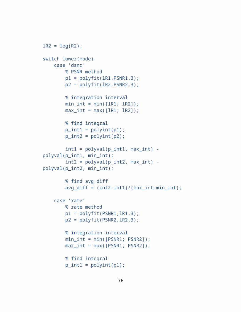
H.264/MPEG-4 PART 10, HEVC, VP6, DIRAC and VC-1 “, Springer , 2014.

35. Y.He , J.Ostermann , M.Domanski , O.C.Au and N.Ling ,"Introduction to the issue on

video coding : HEVC and beyond ", IEEE journal of selected topics in signal processing,

Vol. 7, no. 6 ,Dec 2013.

36. Information about quad tree structure of HEVC

http://codesequoia.wordpress.com/2012/10/28/hevc-ctu-cu-ctb-cb-pb-and-tb/

37. X. Cao, C. Lai and Y.He,“Short distance intra coding scheme for HEVC”, Picture

Coding Symposium, pp. 501-504, 2012.

38. HEVC reference software HM 13.0 [online].

http://hevc.kw.bbc.co.uk/svn/jctvc-a124/branches/

39. X. Li et al, “Rate-Complexity-Distortion evaluation for hybrid video coding”, IEEE

Transactions on Circuits and Systems for Video Technology, vol. 21, pp. 957 - 970, July

2011.

40. HEVC test sequences: ftp://ftp.tnt.uni-hannover.de/testsequences

41. C. Zhaepong, W. Dujuan, J. Guang and W. Chengke, “Octagonal Search Algorithm

with Early Termination for Fast Motion Estimation on H.264”, IAS Fifth International

Conference on Information Assurance and Security, vol. 1, pp. 123-126, 2009

78

42. N. Ling, “High efficiency video coding and its 3D extension: A research

perspective,” ,7th IEEE conference on Industrial Electronics and Applications (ICIEA), pp.

2150-2155, July 2012

43. S. Lui et al, “Video Prediction Block Structure and the Emerging High Efficiency Video

Coding Standard”, IEEE proceedings on Signal & Information Processing Association

Annual Summit and Conference(APSIPA ASC), 2012 Asia-Pacific, pp.1-4, 2012.

44. Basics of video: http://lea.hamradio.si/~s51kq/V-BAS.HTM

45 MPL website: http://www.uta.edu/faculty/krrao/dip/

46. Website for downloading test sequences:

https://media.xiph.org/video/derf/

47. G. J. Sullivan et al, “Standardized extensions of high efficiency video coding (HEVC)”,

IEEE Journal on Selected Topics in Signal Processing, v 7, n 6, p 1001-1016, Dec. 2013.

48 Special issue on emerging research and standards in next generation video coding,

IEEE trans. CSVT, vol. 22, pp. 1646-1909, Dec. 2012.

49. M. T. Pourazad et al,” HEVC: The new gold standard for video compression”, IEEE

CE magazine, vol. 1, issue 3, pp. 36-46, July 2012.

50. HEVC encoded bitstreams:

79

ftp://ftp.kw.bbc.co.uk/hevc/hm-11.0-anchors/bitstreams/

51. V.Sze, M. Budagavi, G.J.Sullivan, “High Efficiency Video Coding:Algorithm and

architectures”, Springer, 2014.

52. G. Bjontegaard, “Calculation of average PSNR differences between RD-curves”,

Q6/SG16,Video Coding Experts Group (VCEG), April 2001.

53. BD metric code [online]. Available.

http://www.mathworks.com/matlabcentral/fileexchange/27798-bjontegaardmetric/

content/bjontegaard.m

54. “Complexity reduction for intra mode selection in HEVC using OpenMP”. This thesis

describes how parallel processing using OpenMP can be used for intra mode selection in

HEVC, M. S. Thesis, EE Dept.,UTA, Arlington, Tx, Dec. 2014

http://www.uta.edu/faculty/krrao/dip/

80

Biographical Information

Jayesh Dubhashi was born in Mumbai, Maharashtra, India in 1990. After

completing his schooling at Parle Tilak Vidyalaya, Mumbai in 2006, he went on to obtain

his Bachelors Degree in Electronics Engineering from Fr. Conceicao Rodrigues College

of Engineering in 2012.

He enrolled at the University of Texas at Arlington to pursue his Master of

Science in Electrical Engineering in the Fall 2012. While at the university he joined the

Multimedia Processing Lab. He worked as an intern in the kinetis MCU Systems and

architecture team for the summer of 2014 and was invited back to coop for the Fall 2014.

81