acomparison of cost structures in japan and the u.s. · acomparison of cost structures in japan and...

Journal of Applied Input-Output Analysis, Vol.2, No.2, 1995

A Comparison of Cost Structures in Japan and the U.S.

Using Input-Output Tables1

By

Kiyoshi Fujikawa*, Hiroshi Izumi* and Carlo Milana**

Abstract

This paper attempts to explain why prices are systematically higher in Japan than in the

U.S. It is aimed at measuring direct and indirect productivity and input-price components

of sectorial costs of production in Japan relative to the U.S. and presenting a methodology

for a bilateral comparison of cost structure by using harmonized input-output tables and

Purchasing Power Parity data. The empirical application reveals new elements that explain

the difference in costs of production between Japan and the U.S. The main finding is

that only in a few industries was the "direct" cost efficiency higher in Japan than in the

U.S. during 1985, but even in these industries the "indirect" productivity component was

significantly lower than that in the U.S.

1. Introduction

International competitiveness and trade disequilibrium between Japan and the United States

have been thoroughly examined by many empirical studies. Among these, the path-breaking

works carried out by Dale W. Jorgenson and his associates have established a methodology which

has become standard in the economic literature aimed at accounting for intercountry differencesin the rates of change and the levels of sectorial costs of production. The methodology was

originated by Jorgenson and Nishimizu (1978), who established a theoretical framework fora bilateral comparison of aggregate economic growth in Japan and the U.S. Jorgenson and

Nishimizu (1981) extended this analysis at the industry level for the first time by measuring therelative sectorial values of production and relative productivity. The most recent studies in thisfield are those made by Jorgenson and Kuroda (1990), Jorgenson, Sakuramoto, Yoshioka, andKuroda (1990), Fuss and Waverman (1991), Nakamura (1991), Jorgenson and Kuroda (1992),and Denny, Bernstein, Fuss, Nakamura, and Waverman (1992)2. These studies compare costsof production by taking into account the direct input cost components.

The unit cost of an industry's output in a country relative to the unit cost of another countryis explained by decomposing it into differences in primary and intermediate input prices andproductivity levels in the same industry of the two countries. The output and input prices,

Manuscript received January 13, 1995. Revised August 8, 1995.* Osaka University of Economics

** ISPE (Institute of Studies for Economic Planning), Italy.

JAn earlier version of this paper has been prepared for the 1994 Conference of the Pan Pacific Association of Input-Output Studies, Tokyo, 12-13 November 1994. We are deeply grateful to Masahiro Kuroda forhaving provided us with the data on Japan-U.S. relative prices of outputs and inputs and to Ichiro Tokutsuand an anonymous referee for their constructive comments. This research has been financially supported bvOsaka University of Economics and the Italian National Research Council (CNR) within the Strategic Project"Technological Change and Industrial Growth".

2See Jorgenson (1988) for an overview of previous analyses. A more descriptive analysis is provided by vanArt and Pilat (1993) and Pilat and van Art (1994). Among other studies that are not concerned directly withthe analysis of relative cost and productivity levels but focus their attention on the international comparison ofinput substitution and technical change, see the recent works made by Boskin and Lau (1992) and Saito andTokutsu (1992)(1993).

2 Journal of Applied Input-Output Analysis, Vol.2, No.2, 1995

relative to those in the reference country, are measured by using sectorial Purchasing Power

Parities (PPP). The intercountry difference in sectorial costs of production is accounted for

with a good degree of approximation by postulating a sufficiently general functional form of

the production or cost function. In the above-mentioned studies this function has a Translog

functional form, which is applied either directly after having been econometrically estimated or

implicitly by using Tornqvist index numbers. Diewert (1976), in fact, showed that, when there

is no variation in technology, there is an exact correspondence between Translog production (or

cost) functions and aggregating Tornqvist index numbers of input quantities (or prices). Vari

ations in productivity may be represented by the "implicit" Tornqvist index number obtained

by the difference between production (or cost) variations and the aggregating Tornqvist index

numbers of differences in input quantities (or prices) 3.

The novelty of this paper is the extension of the above-mentioned methodology to the input-

output framework, which permits us to analyze, not only the direct, but also the indirect input

components of costs of production which are incorporated in the intermediate inputs. More

specifically, whereas the studies mentioned above have left the costs of intermediate inputs

"unexplained," the techniques of input-output analysis permits us to decompose these costs

into indirect input price and technological components. The distinction of the analyses based

on direct costs of production from those based on direct and indirect costs is related, respectively,

to the concepts of "industry" and the so-called "vertically integrated sector". As we shall see,

both concepts are familiar in 1-0 analysis and have always been employed in the economic

literature, although their definition has seldom been explicitly established4.

Moreover, by adopting the approximating Translog functional form of sectorial cost functions,

we are able to consider a modified Leontief price equation system, where the physical input-

output coefficients may vary according to this particular functional form. Since the Translog cost

function includes the Cobb-Douglas cost function as a special case, our input-output equations

represent a generalization of Klein's (1952-53) reformulation of Leontief's input-output system.

The comparative study of cost structure was carried out on the input-output tables for Japan

and the U.S., which were harmonized by adopting the same sectorial classification.

In the following section we present the methodology of decomposing differences in costs of

production in the intertemporal and interspacial comparisons within the input-output frame

work. In section 3, we present the application of the decomposition based on the Translog-

Tornqvist representation of the technology of sectorial price differences between Japan and the

U.S. in the year 1985. Section 4 provides the concluding remarks.

2. Accounting for Cost Differences in the Intertemporal and Interspa

cial Comparisons

The international and interspacial comparisons of cost structure can be based on accounting

methods which are basically the same as those developed for intertemporal comparisons. Let's

start by considering the decomposition of the time-change of an aggregate value as follows:

dVt d dx

where Vt = J2iLi wa 'xit = wt *xt is tne sum of values obtained by multiplying the prices wit bythe quantities xiti for i — 1,..., N, and t means that they are considered as functions of time (wt

3 Denny and Fuss (1983), however, have shown that the direct application of econometrically estimated

Translog production (or cost) functions is not always equivalent to the application of Tornqvist index num

bers. In fact, the Tornqvist index numbers of productivity difference correspond exactly (in Diewert's sense) to

the measure obtained using the underlying Translog functions only if these differ in their "first-order" parameters.

4 See Pasinetti (1973) for an extensive discussion of the concept of vertical integration in economic analysis.

A Comparison of Cost Structures in Japan and the U.S. 3

and xt represent column vectors of prices and quantities at time t, respectively, and ' denotes

transposition). Two main accounting methods for intertemporal comparisons can be devised

starting from equation (1) and following the so-called Bennet (1920) decomposition procedure

and the Divisia (1925) index number approach. Denny and Fuss (1983b) provided a justification

for extending these methods to interspacial comparisons.

2.1. The Bennet decomposition procedure in the I-O accounting for cost changes

Integrating both sides of (1) from period 0 to period 1 yields:

(2)

Bennet (1920; p.457) discrete-time approximations to the two sums of integrals in decomposition (2) are given by

aw = (W; - w;)i(Xl+x0) ~ ft ^xt ■ dt(3)

;i1

Bennet also showed that the sum of the two approximating variables AW and AX is exactly

equal to the difference in the aggregate value in the two periods, that is:

Vi - Vo = AW + AX (4)

This result can be justified also on the ground of Diewert's (1976, p.118) Quadratic lemma. Thisstates that, for any quadratic function y — f{zuz2).".., zr) such that

/(*l, *2, .-, Zr) = a0 + Zln a™Zm + £„ En *mnZmZn ,-.

where am and amn are constants and amn = anm for all m,n, then

Since Vt = wt-xt is a special case of (5), the corresponding accounting equation for costdifferences between period 1 and period 0 can be written as (4).

In the input-output framework, Vt can be assigned the meaning of a sectorial cost of production and wt and xt assume the meaning of vectors of input prices and input quantities,

respectively. Fujikawa, Izumi, and Milana (1993a)(1993b)(1995) applied the decomposition formula (4) to the changes observed in the accounting Leontief price system, which is expressed in"reduced" form as follows:

If, for each ith output price pit, we replace the vector w^ with the row vector of primary inputprices vt = [vltv2t...vMt] of order M, and the vector xt with ith column of the matrix of order

M x N given by F*(I - A*)"1, where the matrices Ft and At are the Leontief's matrices of


direct input-output coefficients at period f, and apply repeatedly at various stages the same

decomposition procedure described above, we have:

(pi - Po) = AFIM1+AFIM2+AFIM3

= AFIM1A+AFIM1B+AFIM2A+AFIM2B+AFIM3A+AFIM3B ^8^

= AFIM1A+AFIM1B+AFIMT1+AFIMT2

where

AFIM1 = (v1-v0)|[F0(I-Ao)"1 +Fi(I-Ai)"1]: Total primary input price component;

AFIM2=|(vi+vo)(Fi-Fo)|[(I-Ao)"1+(I-Ai)-1]: Total primary input technological

component;

AFIM3 =|(vi + vo)^(F1 + F0)[(I - Ai)""1 - (I - Ao)"1]: Total intermediate input tech

nological component.

These can, respectively, be further decomposed as follows:

AFIM1 =AFIM1A+AFIM1B:

AFIM2 =AFIM2A+AFIM2B

AFIM3 =AFIM3A+AFIM3B

where

AFIM1A = (v1-vo)|(Fo + Fi): Direct primary input price component;

AFIM1B = (v1-v0)|[F0A0(I - Ao)"1 + FiAi(I - Ai)"1]: Indirect primary input pricecomponent;

AFIM2A =|(vi + vo)(Fi - Fo): Direct primary input technological component;

AFIM2B =|(vi + vo)(Fi - F0)^[A0(I - Ao)"1 + Ai(I - Ai)"1]: Indirect primary inputtechnological component;

AFIM3A=|(v1+vo)|(F1-f-Fo)|[(I-Ao)"1+(I-A1)-1](A1-Ao): Direct intermediate

input technological component;

AFIM3B =|(vi + vo)|(Fi + F0)|[(I - Aq)"1 + (I - Ai)"1]^ - A0)|(A0 + Ai).I[(I _ Ao)"1 + (I - Ai)"1]: Indirect intermediate input technological component;

and obtaining also

AFIMT1 =AFIM2A + AFIM3A: Direct total input technological component;

AFIMT2 =AFIM2B+AFIM3B: Indirect total input technological component.

It can be noted that the term (AFIM2+AFIM3) can be defined as the difference in the

unit costs of production after accounting for differences in input prices. By normalizing output

and input prices, so that po= [11...1] and vo= [11...1], and redefining consistently the matrices

Fo, Fi, Ao, and Ai, the cost efficiency (defined as cost ratio) of the vertically integrated sectors

in 1 with respect to the same sectors in 0 is given by

7VIS = [L + AFIM2+AFIM3] (9)

where i is the unit vector [1 1 ... 1].

The cost efficiency of industries in 1 with respect to the respective industries in 0 can be

calculated by taking into account the "direct" technological components, that is

1IND = V + AFIM2A+AFIM3A] (10)

The effect on cost efficiency of vertically integrated sectors arising from the relative productivity

incorporated directly and indirectly into intermediate inputs is given by the ratio

7INTP = TVIS ■ llND (11)


where^denotes a transformation of a vector into a diagonal matrix.

The relative total factor productivity of the vertically integrated sectors in 1 with respect to

those in 0 are expressed as

The total factor productivity of industries in 1 relative to that of industries in 0 is given by

wIND = [U...l]-j^D (13)

Therefore, the relative level of total factor productivity of 1 with respect to 0 can be decomposed

as follows:

— kind • ^intp (14)

where 7TINTP = jJ^TP-

A slightly different procedure can be set up starting from the traditional input-output price

system that is expressed in "structural" form as follows:

(15)

Adopting Bennet's discrete-time approximation given by (4) to the decomposition of time-

change of the output prices in each sector yields:

(Pi " Po) = (Pi - PoH(Ao + Ai) -j- (vi - vo)i(Fo + Fi)

(16)

+AT

where AT = |(p0 +pi)(Ai - Ao) + |(v0 +vi)(Fi - Fo) is the industry "direct" technologicalcomponent.

Expressing the system (16) in "reduced" form by solving it with respect to (pi -p0), through

a simple further manipulation, gives:

(Pi - Po) = AV1 + AV2 + AF1 + AF2 + AA1 + AA2

(17)

= AV1 + AV2 + ATI + AT2

where

AV1 =(vi - vo)|(Fo + Fi): Direct primary input price component;

AV2=(Vl -vo)|(Fo + Fi)|(Ao +Ai) [I - §(A0 + Ai)]"1: Indirect primary input pricecomponent;

AF1 =|(vo + vi)(Fi — Fo): Direct primary input technological component;

AF2 =i(v0 + vi)(Fi - Fo)^(Ao + Ai) [I - |(A0 + Ax)]"*: Indirect primary input technological component;

AA1 =^(po +Pi)(Ai — Ao): Direct intermediate input technological component;

AA2=|(p0 + pi)(Ai - A0)^(A0 + Ai) [i - |(A0 -f-Ai)]"1: Indirect intermediate inputtechnological component;

and

ATI =AF1+AA1 = AT: Direct total input technological component;

AT2 =AF2-fAA2: Indirect total input technological component.

We note that the decomposition (17) approximates the decomposition given by (8), since

AV1 =AFIM1A

AV2 ^AFIMIB

AF1 =AFIM2A


AF2

AA1

AA2

and

ATI ÂFIM2A+AFIM3A

AT2 ÂFIM2B+AFIM3BMoreover, the intermediate input price component in (16) can be reconstructed by using

the indirect input price and technological components in (17), that is (pi - po)|(Ao + Ai) =

AV2 + AT2 = AV2 + AF2 + AA2. This can be approximated by using the corresponding

elements in (8), that is (px - po)|(Ao + Ai) ~ AFIM1B + AFIM2B + AFIM3B5.

The two decomposition procedures (8) and (11) are not,,however, equivalent. The decom

position (8) starts from the reduced form of the accounting price equation system given by

(7), whereas the decomposition (17) calculates the reduced form of the decomposition of price

changes after the decomposition procedure has been applied to the "structural" form of the

accounting equation system. Moreover, we note that the decomposition (8) has the advantage

of avoiding the use of the weights |(po + Pi), which are evidently constructed by using the sameprices that are under examination.

Finally, under the normalization of output and input prices, so that po= [11...1] and vo=

[11...1], and consistent definition of the matrices Fo, Fi, Ao, and Ai, relative cost efficiencies

of vertically integrated sectors and industries are, respectively:

jVIS = [i + (AF1+AF2)+(AA1+AA2)]

(18)

= [i + AT1+AT2]

and

jIND = [i + AF1+AA1]

(19)

= [i + ATl]

The relative total factor productivity measures for the vertically integrated sectors and industries

can be calculated, respectively, by using the above cost efficiency measures in the definitions

(12) and (13).

2.2. The Divisia index number approach in the I-O decomposition of cost changes

The second alternative decomposition method can be derived from the Divisia (1925) index

number approach. Starting from (1) and dividing through by Vt we obtain:

dVt 1 _ d\nVt _ y^ dwu 1dt vt ~ dt ~ Z^=i at • wn '

wax it _J_ dx

N_ wjtxjt * î=1 y" wJtxjt xa *J~l J-' (20)

where sa = ~-^™liXu is the cost share of the ith input at time t. Integrating both sides of

(20) from period 0 to period 1 yields:

5 Commenting on the decomposition procedure (8) proposed in a former version of the paper written by

Fujikawa, Izumi, and Milana (1993a) and presented at the 1993 PAPAIOS Annual Conference, Mitsuo Ezaki

suggested an alternative procedure, which consists of calculating components equivalent to (AVI + AV2),

(AF1 + AF2), and (AA1 + AA2).


lnVi-lnVo = H^

= Ef=1 /o **£»■ ■ «« ■ dt + £f=1 jj S^l . Sii. dt (2i)

Good discrete-time approximations to the two sums of integrals in (21) are given by the

Tornqvist indices

A In W = (In wi - In w^)^ + s0) ~ jj ^^ • s, • dt(22)

AlnX = I(sq + si)(lnxi - lnx0) ~ ft st • ^f^ • dt

We note, however, that unlike Bennet's discrete-time approximations these two Tornqvist

indices do not necessarily sum up exactly to the change of the aggregate value, so that in general

(In V\ — In Vq) / A In W + A \nX. Therefore, if we want to guarantee the exact summing up of

the decomposition procedure and we are approximating, for example, the first sum of integrals

referring to the price components with the Tornqvist price index we must approximate the

second integral by using the so-called implicit Tornqvist quantity index6 given by

jo

^sx +s0) ~ / ^ • ^J^ • dt (23)

where the superscript ~ means that the index number is constructed implicitly by deriving

it from the difference in the log-change of the aggregate value direct index number and the

(weighted) log-changes of direct price indices.

Since the "direct" Tornqvist price index and the "implicit" Tornqvist quantity index always

sum up exactly to the change of aggregate value, we can write

In Vi - In Vo = Aln W + Aln~X (24)

In the framework of the 1-0 price model in reduced form given by (7), this approach gives

rise to the following approximating decomposition procedure:

(25)

= A In FIM1A + A In FIM1B + A lnFIMT

where At = ptAjp"1 and Ft = v^F^p^"1 (for 2=0,1) are the Leontief's direct 1-0 matrices,which are expressed in nominal shares valued at current prices and

AlnFIMlA =(lnvi - Invo)|(Fo + Fi): Direct primary input price component;

A In FIM1B =(ln vi - In vo)| [F0A0(I - Aq)"1 + Pi Ai(I - Ai)"1]: Indirect primary input price component;

Aln^IMT = (Inp! - lnp0) - (InVl - lnvo)i[Po(I - Aq)"1 + F^I - Ai)"1]: implicit(direct and indirect) Tornqvist-type technological component.

We note that the term A lnFIMT can be defined as the logarithmic difference in the unit

costs of production of the vertically integrated sectors, after accounting for differences in input

6 See, for example, Allen and Diewert (1981) for the concept of implicit index numbers.


prices. The relative cost efficiency of sectors in 1 with respect to sectors in 0 are defined as the

ratio of costs that would be obtained after correcting for the effects of differing input prices,

that is:

jVIS = exp(A lnFIMT) (26)

where ~ means that this measure is calculated implicitly by using the implicit index A In FIMT.

The levels of relative total factor productivity of the vertically integrated sectors in 1 with respect

to those in 0 are given by:

TTVIS = [11...1] 'JviS_ (27)

= exp(-AlnFIMT)

In the framework of the 1-0 price model in "structural" form given by (15), the same approach

gives rise to the following approximating decomposition procedure:

(lnpi - lnpo) = (lnpi - lnpo)±(Ao + Ai) + (In vi - In vo)±(Fo + Fi)

_ (28)

+AlnY

whereAln Y is the implicit Tornqvist index of (direct) technological component.

Solving (28) with respect to (lnpi — lnp0), through a further manipulation, yields:

(lnpi - lnp0) = (lnvi - lnvo)|(Fo + Pi) [I - |(A0 + Ai)]"1

+Al^Y.[l-i(Ao + A1)]"1 (29)

= A In VI + A In V2 + A hTTl + A lnT2

where

A In VI =(ln vi — In vo)^(Fo -f Fi): Direct primary input price component;

AlnV2 =(lnvi - In vo)|(Fo + Fi)|(A0 + Ax) [I - |(A0 '+ Ai)] : Indirect primary input

price component;

AlnTl= A In Y =(lnpi - lnpo) - (lnpi - lnpo)|(Ao -h Ai)

—(In vi — Invo)|(Fo + Fi): Direct total input technological component;

AlnT2=AlnTl-^(A0 + Ai) [i - |(A0 + Ai)] : Indirect total input technological com

ponent.

We note that the decomposition (29) approximates the decomposition given by (25), since

AlnVl=AlnFIMlA

AlnV2 /AlnFIMlB

A In Tl + A In T2 ^ A In FIMT..

Moreover, the intermediate input price component in (28) can be reconstructedJ>y using the

indirect input price and technological components in (29), that is (lnpi — lnpo)|(Ao + Ai) =

AlnV2 4- AlnT2.

The implicit measures of relative cost efficiencies of vertically integrated sectors and indus

tries are, respectively, redefined as follows:

jVIS = exp (AlnTl + A lnT2) (30)


(31)

and, following definition (12), the implicit measure of technological component of intermediate

input prices is given by

T/iVTP = exp(AtoT2) (32)

The corresponding implicit measure of relative total factor productivity in vertically integrated

sectors and industries can be calculated, respectively, by using the above cost efficiencies. Re

calling definitions (10) and (13), we have:

wVjs = [11...1] -Jvis = exp(-AlnTl - Aln~T2)(33)

= kind • kintp

where

kind = [11-1] -7ind = exp(-AlnTl) (34)

and

= [11...1] -Jintp = exp(-AlnT2) (35)

In order to clarify some aspects of the methodology described above, we recall some theo

retical foundations from which this stems form. By establishing the Quadratic lemma, Diew-

ert(1976) showedthat if the underlying "aggregator" function Vt = V(wt,0) (which is numer

ically equal to w't • xt, since it is assumed that xt = dVt/dwt and Vt — w^ • {dVt/dwt)), with0= [ao»i»2--■<*nJiiJ12--Inn]1 being a vector of parameters which remain constant over time)has a homogeneous Translog functional form, so that

N N N

In V(wt,0) = ao + ]T a{ In wit + - ]T^ jjk In wjtwkt (36)i=l i = lAr=l

then lnKi-ln Vb = (lnwj -In Wq)^(s0-fsi), that is (In Vi -In Vo) can be exactly reconstructed

by an aggregating Tornqvist index number of prices. In the notation of the 1-0 price model

the function (36) can be re-expressed, for each sector, as pi - exp q(lnpt,ln vt\d), where c,-(-)

has the value of the logarithm of a unit cost function. Therefore, if Q does not change over

time, the log-change of output prices can be exactly decomposed as follows: (lnpi - lnp0) =

(lnpi-lnpo)|(Ao + Ai) + (lnvi-In vo)^(Fo + Fi), that is the log-change of output prices canbe accounted for only by a weighted sum of log-change of input prices, since no technological

change has taken place.

Technological changes are reflected by variations over time of the functional form or the

technological parameters of the "true" unknown function ct-t(ln pt In vt; dt). As Denny, Fuss,

and May (1981) have suggested, this function can be approximated by a function q(ln pt, In

vt,t; Q), which is quadratic in all the explanatory variables, including the technology index t.

The function cu(-) is therefore replaced by C{(•), which is characterized by a Translog functional

form with constant parameters Q and the additional explanatory variable t We also note that

onlyjn the case where cit(\n pt,ln vt;0t) is identically equal to cz(ln pt,ln vtit; 0) for all t's, will

AlnT = (lnpi -lnp0) - (lnpi-lnpo)^(Ao + Ai) - (In vx - In vo)^(Fo +Fi) be exactly equal


to the "true" technological component, otherwise it will only approximate this last component7.

However, even if it is only approximating the "true" unknown technological component, this

implicit measure of magnitude always sum up exactly to the log-change of output prices, by

construction, along with the direct measure of the input-price component.

Moreover, since the Translog function includes the Cobb-Douglas function as a special case,

the use of Tornqvist-type formulas in input-output analysis brings about a generalization of

Klein's (1952-53)(1956) and Morishima's (1956)(1957) reformulation of Leontiefs equation sys

tem8. They used, in fact, constant input-output coefficients expressed as unit cost shares valued

at current prices, rather than technical coefficients valued at constant prices or expressed in phys

ical units, as in Leontiefs system. More specifically, the inverse matrix [I - |(A0 + Ai)]"1 isour Tornqvist-type reformulation of Leontiefs and Klein-Morishima's inverse matrices, where

the technology is described by an underlying Translog cost function. This reformulation permits

us to be consistent with recent applications of studies in the field of intertemporal and inter-

spacial comparison of cost structure. As we mentioned above, these studies were all concerned

with the "direct" costs of production at the industry level, whereas we take into account, not

only the industries and their "direct" costs, but also the so-called "vertically integrated sectors,"

with their "direct" and "indirect" costs of production.

The concepts of "industry" corresponds to the 1-0 equation system (15), which is expressed in

"structural" form using only direct 1-0 coefficients, whereas the concept of "vertically integrated

sector" corresponds to the 1-0 equation system (7), which is expressed in "reduced" form using

direct and indirect 1-0 coefficients. A domestic industry can be defined as an aggregate of

"observed" production units which produce homogeneous goods by using primary inputs (human

and non human capital, labor, imported intermediate inputs, land and natural resources) as well

as domestically produced intermediate inputs, which are originated by other industries producing

different types of goods. On the other hand, a "vertically integrated sector" is an accounting

concept defined as an aggregate of "unobservable" production units which produce homogeneous

goods as final output as well as all the necessary domestically originated intermediate inputs

of various kind by using only primary inputs9. Whilst the costs of production in each industry

and the corresponding vertically integrated sector are the same, their inputs are different: the

industry has to buy from other domestic industries some of the inputs of production (the so-

called domestically produced intermediate inputs), whereas the theoretically defined vertically

integrated sector is completely autonomous and therefore produces itself all the intermediate

inputs that are needed directly and indirectly as well as the final output by using all the necessary

primary inputs. Both concepts are useful for a complete accounting analysis qf the structure of

costs of production.

The distinction between industries and vertically integrated sectors also makes clear the

different implications of the alternative formulas (8), (16), (25), and (29). The functional forms

of the underlying production or cost function that are implied by the particular index number

formulas used in the above four alternative cases refer to different technological hypotheses. More

specifically, in (8) and (25) the index number formulas correspond to a particular functional form

of cost functions in the vertically integrated sectors, whereas in (16) and (29) they correspond

to a particular functional form of cost functions in the "observed" industries. These different

7Since Diewert's Quadratic lemma involves derivatives of cost function with respect to its variables, a problem may arise from the discontinuity of the technology index t between the countries examined in interspacial

comparisons. However, Denny and Fuss (1983b) provided a justification for the application of the Quadratic

lemma in this context.

8See Saito (1972), among others, for the empirical application of this reformulation of Leontiefs system.9 The notion of vertically integrated sector is implicit in various definitions of macroeconomic aggregates

and in many analyses of classical and neoclassical economists. Walras (1874,1877), for example, eliminated

intermediate inputs from his theoretical model by adopting the device of vertical integration. In I-O analysis,

Leontief (1953) (1956) applied empirically this concept for the first time by using his inverse 1-0 matrix (which

was previously defined in Leontief, 1941-1951). For an example of more recent applications see Heimler (1991).


hypotheses on sectorial technology give rise to different results in the alternative decomposition

procedures.

Jorgenson and Kuroda (1990), Fuss and Waverman (1991), Nakamura (1991), Kuroda (1992),

and Denny, Bernstein, Fuss, Nakamura, and Waverman (1992) applied a formula equivalent to

(28) to account for sectorial cost differences between Japan and the U.S., by aggregating the

inputs at the so-called KLEMlevel (Capital, Labor, Energy, and Intermediate inputs). They de

composed the sectorial cost differences into direct input price component, which in our notation

is given by (lnpi-lnpo)|(Ao+Ai) + (In vi -In vo)|(Fo+Ji) = (AJn Vl+Aln V2+AlnT2),

and direct technological difference, which is given by AlnTl=AlnY. Our proposed method

based on (29) decomposes the direct intermediate input price component given by (lnpi —

lnpo)|(Ao + Ai) into the incorporated primary input price component, which is given by

AlnV2, and the incorporated total input technological component, which is given by AlnT2.

At the sectorial disaggregation level of the above-mentioned studies, it is important to decom

pose the direct intermediate input price component, as this often amounts to more than 60 per

cent of the unit cost of production.

3. Empirical Results

In the preceding section we proposed four alternative methods which can be used to account for

differences in sectorial costs of production between two countries. These methods are given by

the formulas (8), (17), (25), and (29) which can lead to slightly different empirical results. Since

we intend to compare our results with those obtained by previous studies in the field, which

were based on the analysis of "direct" input costs by using a formula corresponding to (28), we

shall concentrate mainly on formula (29), which can be derived from (28) as its "reduced" form

and can be brought back to "direct" accounting components.

3.1. Data

The Japanese and U.S. 1-0 tables for the year 1985, which were used in the empirical appli

cation, were harmonized according to the same industrial classification. The sectorial output

and primary input prices of Japan are relative to the respective U.S. prices. The output price

ratios are calculated by using Purchasing Power Parity (PPP) data supplied by OECD for 187

commodities for the year 1985. The PPP data were aggregated to be consistent with the indus

trial classification by using the averages of share weights in the final consumption in the U.S.

and Japan. The PPP data were corrected in order to compare producer prices rather than con

sumer prices. Therefore, they were adjusted by excluding transportation costs and commercial

margins per unit of output. The levels of producer prices relative to the corresponding U.S.

prices (with all prices expressed in a common currency) were actually obtained by dividing the

corrected sectorial PPP data by the observed nominal exchange rate of Japanese Yen against 1

U.S. dollar10. The annual average of the nominal exchange rate in 1985 was 238.54 Yen per U.S.

dollar. Moreover, the original OECD PPP data should refer, ideally, to commodities that have

the same characteristics and quality standards, so that by deflating the current-price sectorial

values of production by means of the obtained corresponding producer prices, we would end up

with quantities and input-output coefficients that include quality differences between the two

countries. In practice, however, we cannot control if quality differences are completely netted

out from those computed producer prices and therefore our empirical results could be affected

by some residual errors in the data11. As for the sectorial labor prices, the ratios between the

Japanese hourly wages expressed in Yens and the U.S. hourly wages expressed in U.S. dollars

10 For an analytical description of this calculation of price ratios, see Fujikawa, Izumi, and Milana (1995)11 We are grateful to an anonymous referee for having reminded us about this point.


(which give us implicitly the sectorial PPP for labor prices) were divided by the nominal ex

change rate in order to obtain the Japanese labor prices relative to the corresponding U.S. labor

prices. The ratios between the sectorial Japanese capital prices relative to the corresponding

U.S. capital prices were derived by those used by Jorgenson and Kuroda (1990) and Kuroda

(1992). The Japanese relative prices of outputs and primary inputs in 1985 are shown in Table

1, where the corresponding sectorial U.S. prices are normalized to 1.

Table 1: Japanese Sectoral Price Index Transformed by Purchasing Power Parities, 1985

(United States Price = 1.000)

Industry

01

02

03

04

05

06

07

08

09

10

11

12

13

14

15

16

17

18

19

20

21

22

23

24

25

26

27

Agriculture

Mining

Oil & Natural Gas

Food Products

Textiles &; Clothing

Paper and Wooden Products

Chemical Products

Coal and Petroleum Products

Non-metal Ores &; Products

Primary Metal

Metal Products

General Machinery

Electric Machinery

Automobiles

Transport Equipment

Precision Apparatus

Other Manufactures

Building Sz Construction

Electricity, Gas, & Water

Wholesale Sz Retail Services

Finance and Insurance

Real Estate Services

Transport Services

Communications

Education &; Medical Services

Other Services

Not Elsewhere Classified

Output

Price

1.8586

2.1645

1.1716

1.4856

1.0056

2.5262

0.7413

1.7544

1.9711

0.7891

0.7560

1.3553

1.0615

0.7984

1.0773

1.2866

1.2910

1.3668

1.4482

0.9304

0.9304

1.1867

0.9816

0.5901

1.9840

1.7954

0.7926

Labor

Input

Price

1.0869

0.4289

0.7144

0.3994

0.5181

0.5038

0.5971

0.4732

0.7307

0.5592

0.4833

0.5235

0.4936

0.3840

0.5515

0.4842

0.5731

0.4910

0.6363

0.7300

0.7105

0.7522

0.5421

1.6183

0.8583

0.4906

0.8955

Capital

Input

Price

1.6070

0.7400

0.7400

1.0260

0.6120

0.7590

1.1880

0.9620

0.2480

3.3950

0.8870

1.9710

1.4190

5.0150

2.5910

0.3510

0.9170

0.7690

0.7860

0.8940

0.8000

0.8000

2.3640

2.3640

0.4820

0.6860

0.6860

Source: Output Price: our computations based on OECD PPP data and nominal exchange rates

Labour Input Price: our computations based on national statistics

Capital Input Price: data made available by Masahiro Kuroda

AComparison

ofCost

StructuresinJapanand

theU.S.

13

Relative

CapitalPrice

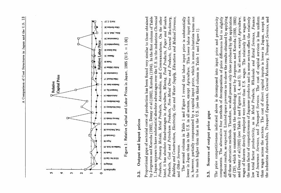
Figure

1:Relative

Capitaland

Labor

Prices

inJapan,

1985

(U.S.=

1.00)

3.2.

Outputandinput

prices

Proportionalgapsofsectorialcostsofproductionhasbeenfound

verysimilartothoseobtained

byJorgensonandKuroda

(1992),Denny

eta/.(1992),

Kuroda(1994).

Inthe

firs

tcolumnofTable

1,JapanappearstohavesubstantialabsoluteadvantagesovertheU.S.in

theindustriesChemical

Products,

Primary

Metals,

Metal

Products,

Automobiles,and

Communications.On

the

other

hand,

ithas

absolutedisadvantages

inAgriculture,

Mining,

Food

Products,Paperand

Wooden

Products,

Coaland

Petroleum

Products,

Non-Metal

Ores

and

Products,

General

Machinery,

Buildingand

Construction,

Elec

tric

ity,

GasandWaterSupply,EducationandMedicalServices,

and

Other

Services.

The

secondcolumn

inTable

1and

Figure

1reveal

that

labor

input

price

issubstantially

lower

inJapanthan

inthe

U.S.

inal

lse

ctor

s,except

Agriculture.

This

lowerlaborinput

price

is,however,

partiallycompensatedby

acapitalinput

pric

e,which

insome

industriesturnsout

tobemuch

higherthan

that

inthe

U.S.

(seethe

thirdcolumn

inTable

1and

Figure

1).

3.3.

Sourcesofoutput

pricegaps

The

price

competitiveness

indicated

above

isdecomposed

into

input

priceand

productivity

components.The

alternativefourmethods

ofdecomposition

ofprice

differences

led

to

slightly

differentresults,

asexpected.

Limitedspacepreventsustoshowtheresultsobtainedbyapplying

allthesealternativemethods.

Therefore,we

shallpresentonlythoseproducedbytheapplication

of

(29),which

isconsistentwiththemethodologyusedbyJorgensonandKuroda

(1990,

1992)

andDenny

eta/.(1992

)(see

Table

2and

Figures

2,4,

and

5).

In

allse

ctor

s,except

Agriculture,

wages

oflaborers

directlyemployedwere

lowerthan

U.S.wages.The

relativelylowwages

are

themain

factorofcompetitivenessofJapaneseproductsand

insome

sectors

offs

etthe

relatively

low

total

factor

productivity,

as

inMetal

Products,

Wholesale

and

Retail

Services,

Finance

and

Insurance

Services,and

Transport

Services.

The

cost

of

capital

services

isle

ssuniform

than

wages

across

the

sectors.

The

cost

of

direct

capital

inputs

islower

inJapan,

except

in

theindustriesAutomobiles,

TransportEquipments,

GeneralMachinery,

Transport

Services,and


Communications, where it is substantially higher, and in Food Products, Primary metals, Metal

Products, and Electric Machinery, where it is approximately at the same level as in the U.S.

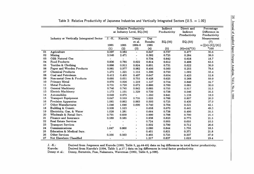
The relative productivity at industry level is similar to that found in the other studies in

almost all sectors (see Table 3 and Figure 3). However, our estimates for Paper and Wooden

Products, Electric Machinery, Transportation Equipment, and Precision Apparatus are rather

different from those of Jorgenson and Kuroda (1990, 1992) and Denny et al. (1992). In general,

according to our results, total factor productivity is lower in Japan than in the U.S. in the

majority of industries, but it is substantially higher in Chemical Products, Automobiles, and

Communications. In the Automobiles industry, however, the relatively high level of productivity

is almost offset by a relatively high cost of capital. The strong competitiveness of Japan in this

industry is therefore mainly due to wages which are lower than that in the U.S.

In almost all sectors, the intermediate input price component is higher in Japan than in

the U.S., thus partially offsetting the primary input price component in many sectors. The

breakdown of the intermediate input price component into primary input price and productivity

components reveals that the productivity incorporated in intermediate inputs used by Japanese

industries is much lower than that in the U.S. In no industry, at the level of aggregation of

our analysis, has this component turned out to be higher in Japan than in the U.S. It is worth

noting that in some industries, like Chemical Products, Primary Metals, Transport Equipment,

and Other Industries (n.e.c), the direct productivity component is higher in Japan than in the

U.S., but is completely offset by the lower indirect productivity component. In Primary Metals

and Transport Equipment the indirect productivity component more than offsets the direct

productivity component, thus leading to an unfavorable total productivity component. In these

cases, the vertically integrated sector presents an overall productivity, which is opposite to the

direct productivity component that is observed superficially at the industry level. Therefore,

with the results reported above, the taxonomy in terms of technological gaps of Japan with

respect to the U.S., as defined at the industrial level by Jorgenson and Kuroda (1992, pp. 44-45,

Table 5), should be revised substantially if we consider it at the level of the so-called "vertically

integrated sectors".

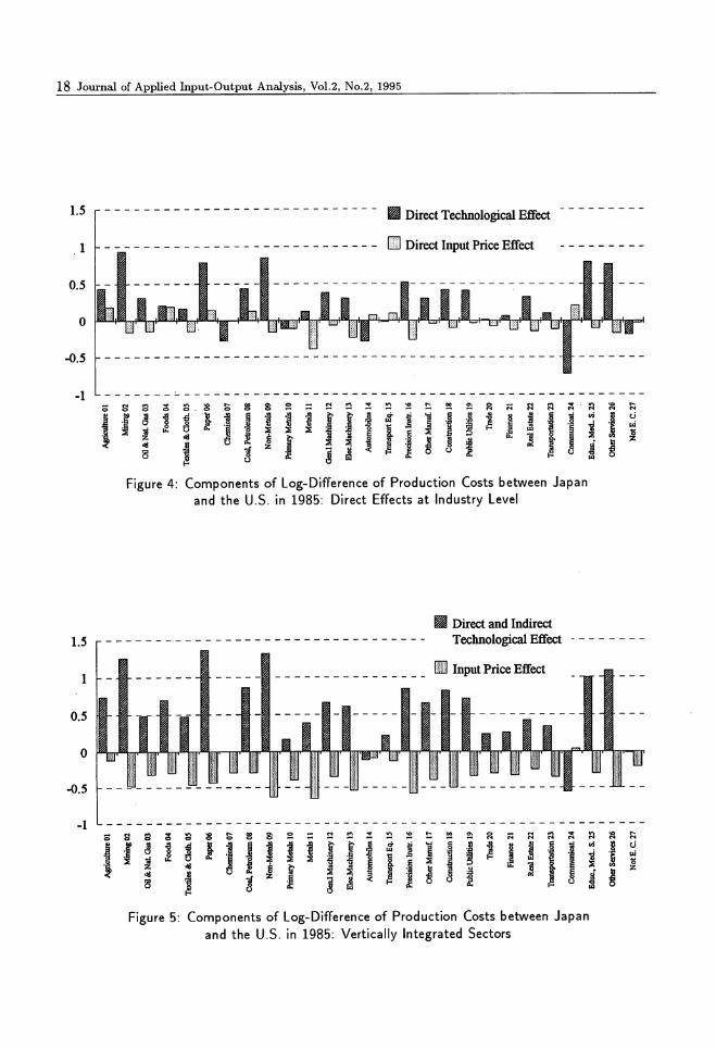
Table 2 as well as Figures 4 and 5 show that the relative cost efficiency of industries is

apparently higher than vertically integrated sectors. Relatively low levels of productivity and

inexpensive primary input prices characterize the production conditions in Japan that are "be

hind the scenes" of the single industries. As Figures 6 and 7 show, productivity in Japan relative

to the U.S. can turn out to be very different if we measure it at the level of vertically integrated

sectors instead of at the industry level. For example, it is 80 per cent higher at the industry

level than at the level of vertically integrated sector in the case of Paper and Wooden Products.

In 17 industries out of 27, relative productivity at the industry level is equal or greater than

30 per cent of productivity measured at level of the corresponding vertically integrated sectors.

This means that international as well as intertemporal comparisons of cost efficiency or relative

productivity levels cannot be complete if they remain confined at the "superficial" analysis of

direct "industrial" costs.

In summary, our results indicate that only in a few manufacturing industries is the "direct"

productivity level higher in Japan than in the U.S. However, in these industries the "indirect"

productivity component is significantly lower than that in the U.S., thus bringing the Japanese

technical performance observed in most sectors during 1985 at a lower level than that in the

U.S.

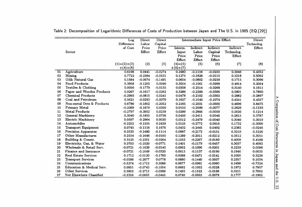
Table 2: Decomposition of Logarithmic Differences of Costs of Production between Japan and The U.S. in 1985 (EQ.(29))

01

02

03

04

05

06

07

08

09

10

11

12

13

14

15

16

17

18

19

20

21

22

23

24

25

26

27

Sector

Agriculture

Mining

Oil& Natural Gas

Food Products

Textiles & Clothing


Chemical Products

Coal and Petroleum

Non-metal Ores & Products

Primary Metal

Metal Products

General Machinery

Electric Machinery

Automobiles

Transport Equipment

Precision Apparatus

Other Manufactures

Building & Constr.


Wholesale & Retail Serv.



Transport Services

Communications

Education & Medical Serv.

Other Services


Log

Difference

of Cost

+(4)+ (8)

0.6198

0.7722

0.1584

0.3958

0.0056

0.9267

-0.2993

0.5621

0.6786

-0.2369

-0.2797

0.3040

0.0597

-0.2252

0.0745

0.2520

0.2554

0.3125

0.3703

-0.0721

-0.0721

0.1712

-0.0186

-0.5274

0.6851

0.5852

-0.2324

Direct

Labor

Price

Effect

(2)

0.0441

-0.2384

-0.0674

-0.1200

-0.1779

-0.1617

-0.0815

-0.0293

-0.1802

-0.1679

-0.3952

-0.1955

-0.2964

-0.1555

-0.1116

-0.2480

-0.1646

-0.2351

-0.1020

-0.1639

-0.1649

-0.0120

-0.2877

-0.1713

-0.0743

-0.2713

-0.0663

Direct

Capital

Price

Effect

(3)

-0.0274

-0.0531

-0.1491

0.0040

-0.0135

-0.0262

0.0241

-0.0070

-0.2052

0.0350

0.0239

0.0758

0.0030

0.2429

0.1676

-0.1114

-0.0100

-0.0264

-0.0771

-0.0140

-0.0320

-0.1783

0.0778

0.3086

-0.1054

-0.0589

-0.0445

Intermediate Input Price

Interm.

Input

Price

Effect

+ (6)+(7)

0.1680

0.1275

0.0654

0.3054

0.0358

0.3286

0.0478

0.1627

0.2165

0.0153

0.0299

0.0450

0.0512

0.0125

0.0432

0.0887

0.1289

0.1553

0.1401

0.0962

0.0613

0.0388

0.0880

0.0677

0.0692

0.1493

0.0746

Indirect

Labor

Price

Effect

(5)

-0.1116

-0.1828

-0.0802

-0.1561

-0.2514

-0.2209

-0.2102

-0.1540

-0.2031

-0.2599

-0.2866

-0.2411

-0.2479

-0.2772

-0.2445

-0.2172

-0.2011

-0.2267

-0.1179

-0.1096

-0.1137

-0.0471

-0.1440

-0.0961

-0.1052

-0.1522

-0.0952

Indirect

Capital

Price

Effect

(6)

-0.0250

-0.0115

-0.0259

-0.0299

-0.0268

-0.0306

-0.0302

-0.1074

-0.0500

-0.0077

-0.0059

0.0046

-0.0040

0.0915

0.0492

-0.0151

-0.0212

-0.0189

-0.0457

-0.0201

-0.0196

-0.0141

-0.0037

-0.0060

-0.0228

-0.0196

-0.0079

Effect

Indirect

Technolog.

Effect

(7)

0.3046

0.3218

0.1715

0.4914

0.3140

0.5801

0.2882

0.4241

0.4696

0.2829

0.2626

0.2815

0.3040

0.1732

0.2385

0.3210

0.3512

0.4009

0.3037

0.2259

0.1946

0.1000

0.2357

0.1698

0.1972

0.3211

0.1777

Direct

Technolog.

Effect

(8)

0.4352

0.9362

0.3096

0.2064

0.1611

0.7860

-0.2897

0.4357

0.8475

-0.1193

0.1214

0.3787

0.3019

-0.3000

-0.0246

0.5226

0.3011

0.4188

0.4092

0.0096

0.0635

0.3226

0.1034

-0.7324

0.7957

0.7662

-0.1962

O

I

o

O

8

W

|

fc

in

01

02

03

04

05

06

07

08

09

10

11

12

13

14

15

16

17

18

19

20

21

22

23

24

25

26

27

Table 3: Relative Productivity of

Industry or Vertically Intergrated Sector

Agriculture

Mining

Oil& Natural Gas

Food Products

Textiles & Clothing


Chemical Products

Coal and Petroleum

Non-metal Ores & Products

Primary Metal

Metal Products

General Machinery

Electric Machinery

Automobiles

Transport Equipment

Precision Apparatus

Other Manufactures

Building & Constr.


Wholesale & Retail Serv.



Transport Services

Communications

Education & Medical Sery.

Other Services


Japanese Industries and

at

J.-K.

1985

(1)0.597

2.540

0.836

0.886

0.981

1.275

0.412

0.695

0.970

0.731

0.746

1.173

0.949

0.647

1.061

1.046

0.508

1.028

0.791

0.589

-

-

1.047

-

0.566

-

Vertically

Relative Productivity

, Industry Level, EQ.(34)

Kuroda

1985

(2)0.582

2.471

_

0.785

0.912

0.977

1.221

0.405

0.651

0.926

0.720

0.745

1.191

0.975

0.559

0.862

1.646

1.523

1.281

0.839

0.585

-

-

0.800

-

0.563

-

Denny

etal.

1984-6

(3)-

-

_

0.622

0.824

0.982

1.115

0.407

0.755

1.219

0.672

0.842

1.329

_

0.735

0.883

0.690

-

-

_

_

-

-

-

-

-

-

Our

Results

1985

(4)0.647

0.392

0.734

0.814

0.851

0.456

1.336

0.647

0.428

1.127

0.886

0.685

0.739

1.350

1.025

0.593

0.740

0.658

0.664

0.990

0.938

0.724

0.902

2.080

0.451

0.465

1.217

Integrated Sectors (U.S. =

Indirect

Productivity

EQ.(35)

(5)0.737

0.725

0.842

0.612

0.731

0.560

0.750

0.654

0.625

0.754

0.769

0.755

0.738

0.841

0.788

0.725

0.704

0.670

0.738

0.798

0.823

0.905

0.790

0.844

0.821

0.725

0.837

Direct and

Indirect

Productivity

EQ.(33)

(6)=(4)*(5)

0.477

0.284

0.618

0.498

0.622

0.255

1.002

0.423

0.268

0.849

0.681

0.517

0.546

1.135

0.807

0.430

0.521

0.441

0.490

0.790

0.773

0.655

0.712

1.755

0.371

0.337

1.019

1.00)

Percentage

Difference in

Productivity

Measurement

(7)= {[(4)-(6)]/(6)}

*100

35.6

38.0

18.7

63.5

36.9

78.6

33.4

52.8

59.9

32.7

30.0

32.5

35.5

18.9

26.9

37.9

42.1

49.3

35.5

25.3

21.5

10.5

26.6

18.5

21.8

37.9

19.4

Oi

c_

O

I-8,

>

liedI1o

I>

I<<CA

to

fJ°

CDCDen

J. -K.: Derived from Jorgenson and Kuroda (1992, Table 5, pp.44-45) data on log differences in total factor productivity.

Kuroda: Derived from Kuroda's (1994, Table 3, p.17 ) data on log differences in total factor productivity.

Denny et al.: Denny, Bernstein, Fuss, Nakamura, Waverman (1992, Table 6, p.599).

A Comparison of Cost Structvires in Japan and the U.S. 17

Relative Difference in

Output Prices ((JP-US)/US)

Direct and Indirect

Productivity in Japan

(US=1.0)

- 6 * ! « ^ 8 »

Figure 2: Difference in Output Prices and Productivity

40 -

30-

20 "

0

-10

II Jorgenson-Kuroda

- □ Denny et al.

H Fujikawa-Izumi-Milana

-30 --

-40-

-50-

-6OL

I

Figure 3: Comparison of Estimations of Relative Difference in Productivity

between Japan and the U.S. ((JP-US)/US)


1.5

1

Direct Technological Effect

Direct Input Price Effect

Figure 4: Components of Log-Difference of Production Costs between Japan

and the U.S. in 1985: Direct Effects at Industry Level

1.5

0.5

0

-0.5

-1

Direct and Indirect

Technological Effect

Input Price Effect

8 2 8 JS

s i22 2 s s a a

Figure 5: Components of Log-Difference of Production Costs between Japan

and the U.S. in 1985: Vertically Integrated Sectors


Figure 6: Relative Direct and Indirect Productivity in Japan, 1985 (U.S. = 1.00)

80

70

60

50

40

30

20

10

0 iis s s s s

I 3 1 * 1I * & o s

§82 = 22222

I

Figure 7: Difference in Measurement of Relative Productivity Levels

between Japan and the U.S. in 1985

(Percentage Difference of Productivity between Industries and Vertically Integrated Sectors)


4. Conclusion

The bilateral comparison between Japan and the United States of relative levels of sectorial

unit production costs and their components has been carried out for the year 1985 by using

harmonized input-output tables and Purchasing Power Parities. The analysis aimed at finding

additional results that would complement those of previous studies in this field. It examined,

not only the direct costs of production at the industry level, but also the indirect costs that

are incorporated in the intermediate inputs. Input-output analysis permits us to decompose

intermediate input costs into primary input price and technological components, thus giving a

further insight into the structure of costs of production. By using an input-output inverse matrix,

which is defined in such a way that it is exactly consistent with the technological assumptions

of the previous studies, we were able to replicate the results of these studies and extend them to

the so-called "vertically integrated sectors". The relative productivity gap between Japan and

the U.S. in 1985 turns out to be much higher if we consider the whole economic system that is

behind the production of the single goods rather than that observable at the industry level.

In particular, Japan seems to have been more competitive than the U.S. in 1985 in few

sectors (Chemicals, Primary Metals, Metals, Automobiles, Trade, Finance, Transport Services,

Communications, and Others not elsewhere classified). This higher competitiveness was mainly

due to lower labor input prices in Japan than in the U.S. This result is more evident in the

analysis carried out on the vertically integrated sectors, where both the input prices and cost

efficiency are much lower that those found at the industry level.

A natural possible extension of this study is in the direction of intertemporal bilateral and

multilateral comparisons of relative cost and productivity levels. The availability of harmonized

input-output tables of Japan, the U.S. and the major European countries for different years

starting from 1970 makes it possible to apply the methodology established in this paper to the

comparison of cost structures of single pairs of countries in different periods of time. Multilateral

comparisons can be made by using appropriate weighted averages of the results obtained in these

bilateral comparisons.

Appendix

Data sources

The list of data sources for the comparison of cost structures in the 1-0 tables of Japan and the

U.S. is the following:

A. Prices by commodity

OECD, "Purchasing Power Parities and Real Expenditures 1985," Paris, (less than 60 items,

aggregates and sub-aggregates);

OECD, PPP data 1985, Paris, on diskettes (187 commodities).

Except the sectors mentioned below, the PPP data were aggregated into the 27 sectors of

the input-output tables by using geometric weighted formulae. Since the PPP data are

purchaser prices, they should be adjusted to the level of producer prices in order to be used

to deflate the input-output table of each country. The data on prices of steal products of

Japan and the U.S. were taken from World Steel Intelligence, 1992 (price of cold-reduced

coil at April 1985). More specifically, for Japan the weighted average of Big Buyer Price

(40% weight) and Dealer Price (60% weight) has been used. PPP data for the whole GDP

were used as proxies for prices of Trade and Finance sectors.


B. Nominal exchange rate between Japan and the U.S. for the year 1985

International Monetary Fund, International Financial Statistics, Washington, D.C.

C. Input-Output tables

USA: Department of Commerce, "Annual Input-Output Accounts of the U.S. Economy," Sur

vey of Current Business, January 1990.

Japan: Management and Coordination Agency, Input-Output Table 1985, Tokyo, 1990.

The sectorial classifications of the Japanese and U.S. 1-0 tables were harmonized according to

the same sectorial classification.

D. Wages by industry

USA: Department of Commerce, "National Income and Product Accounts," Survey of Current

Business, July 1987.

Japan: Management and Coordination Agency, 1985 Input-Output Tables, Tokyo, 1989.

Wages were calculated dividing the value of compensation of employees by the number of

employees.

E. Persons in production activities

Japan: Management and Coordination Agency, Input-Output Tables, 1985 (Employment ta

ble), Tokyo, 1989.

USA: Department of Labor, Time Series Data for Input-Output Industries, Washington, D.C,

1989.

F. Average annual working hours

Japan: (i) Ministry of Labour, Monthly Labour Survey, Tokyo, 1985; (it) Management and Co

ordination Agency, Labour Force Survey, Tokyo, 1985. If the sectorial data were available

in source (i), the average annual working hours of employee were obtained by multiplying

them by 12. Otherwise, the average weekly working hours published in source (it) have

been multiplied by 52.1.

USA: Department of Labor, Time Series Data for Input-Output Industries, Washington, D.C,

1989.

G. Capital input prices

Japan: Capital input prices at the industry level relative to those of the U.S. in 1985 are those

used by Jorgenson and Kuroda (1990) and Kuroda (1994).


References

[1] Allen, R.C. and W.E. Diewert (1981), "Direct Versus Implicit Superlative Index Number Formu

lae," Review of Economics and Statistics 63: 430-435.

[2] Bennet, T. L. (1920), "The Theory of Measurement of Changes in Cost of Living," Journal of the

Royal Statistical Society 83: 455-462.

[3] Boskin, M. J. and L.J. Lau (1992), "International and Intertemporal Comparison of Productive

Efficiency: An Application of the Meta-Production Function Approach to the Group-of-Five Coun

tries," Economic Studies Quarterly 43: 298-312.

[4] Denny, M., J. Bernstein, M. Fuss, S. Nakamura, and L. Waverman (1992), "Productivity in Man

ufacturing Industries, Canada, Japan and the United States, 1953-1986: Was the 'Productivity

Slowdown' Reversed?," Canadian Journal of Economics 25: 584-603.

[5] Denny, M. and M. Fuss (1983a), "A General Approach to International and Interspacial Produc

tivity Comparisons," Journal of Econometrics 23: 315-330.

[6] Denny, M. and M. Fuss (1983b), "The Use of Discrete Variables in Superlative Index Number

Comparisons," International Economic Review 24: 419-421.

[7] Denny, M., M. Fuss, and D. May (1981), "Intertemporal Changes in Regional Productivity in

Canadian Manufacturing," Canadian Journal of Economics 14: 390-408.

[8] Diewert, W.E. (1976), "Exact and Superlative Index Numbers," Journal of Econometrics 4: 115-45.

[9] Divisia, F. (1925), "L'indice monetaire et la theorie de la monnaie," published in three parts in

Revue d'Economie Politique 39: 842-861, 980-1008, and 1121-1151.

[10] Fujikawa, K., H. Izumi, and C. Milana (1993a), "Origin of Price Difference between Japan and

USA," Osaka Keidai Ronshu 43: 231-243 (in Japanese).

[11] Fujikawa, K., H. Izumi, and C. Milana (1993b), "International Comparison of Cost Structure,"

Osaka Keidai Ronshu 44: 211-235 (in Japanese).

[12] Fujikawa, K., H. Izumi, and C. Milana (1995), "Multilateral Comparison of Cost Structures in

the Input-Output Tables of Japan, the U.S. and West Germany," Economic Systems Research

(forthcoming).

[13] Fuss, M. and L. Waverman (1991), Costs and Productivity in Automobile Production: A Compari

son of Canada, Japan and the United States, Cambridge University Press, Cambridge.

[14] Heimler, A. (1991), "Linkages and Vertical Integration in the Chinese Economy," Review of Eco

nomics and Statistics 73: 261-267.

[15] Jorgenson, D.W. (1988), "Productivity and Economic Growth in Japan and the United States,"

American Economic Review 78: 217-22.

[16] Jorgenson, D.W. and M. Kuroda (1990), "Productivity and International Competitiveness in Japan

and the United States, 1960-1985". In C. R. Hulten (ed. by), Productivity Growth in Japan and the

United States, NBER, Studies in Income and Wealth 53, The University of Chicago Press, Chicago,

pp.29-57.

[17] Jorgenson, D.W. and M. Kuroda (1992), "Productivity and International Competitiveness in Japan

and the United States, 1960-1985," Journal of International and Comparative Economics, 1992, 1:

29-54 (reprinted in Economic Studies Quarterly, 1992, 43: 313-325).

[18] Jorgenson, D.W. and M. Nishimizu (1978), "U.S. and Japanese Economic Growth, 1952-1974: An

International Comparison," Economic Journal 88: 707-726.

[19] Jorgenson, D.W. and M. Nishimizu (1981), "International Differences in Levels of Technology:

A Comparison between U.S. and Japanese Industries". In International Roundtable Conference

Proceedings, Institute of Statistical Mathematics, Tokyo.

[20] Jorgenson, D.W., H. Sakuramoto, K. Yoshioka, and M. Kuroda (1990), "Bilateral Models of Pro

duction for Japanese and U.S. Industries," in C. Hulten (ed. by), Productivity Growth in Japan

and the United States, NBER, Studies in Income and Wealth 53, The University of Chicago Press,

Chicago, pp. 59-83.


[21] Klein, L. R. (1952-53), "On the Interpretation of Professor Leontief's System," Review of Economic

Studies 20: 131-136.

[22] Klein, L. R. (1956), "The Interpretation of Leontief's System: A Reply," Review of Economic

Studies 24: 69-70.

[23] Kuroda, M. (1994), "International Competitiveness and Japanese Industries, 1960-1985," Discus

sion Paper, Keio Economic Observatory, Tokyo, Japan.

[24] Leontief, W. (1941), The Structure of American Economy 1919-1929, Cambridge University Press,

Cambridge, Mass. (2nd Edition: The Structure of American Economy 1919-1939, Oxford Univer

sity Press, New York, 1951.)

[25] Leontief, W. (1953), "Domestic Production and Foreign Trade: The American Capital Position Re-

examined," Proceedings of the American Philosophical Society 97: 332-49.(Reprinted in Economia

Internazionale, February 1954, 7: 9-38.)

[26] Leontief, W. (1956), "Factor Proportions and the Structure of American Trade: Further Theoretical

and Empirical Analysis", Review and Economics and Statistics 38: 386-407.

[27] Morishima, M. (1956), "A Comment on Dr. Klein's Interpretation of Leontief's System," Reviewof Economic Studies 24: 65-68.

[28] Morishima, M. (1957), "Dr. Klein's Interpretation of Leontief's System: A Rejoinder," Review ofEconomic Studies 25: 59-61.

[29] Nakamura, S. (1991), "Explaining Cost Differences between Germany, Japan, and the United

States," in W. Peterson (ed. by), Advances in Input-Output Analysis. Technology, Planning, and

Development, Oxford University Press, Oxford, pp. 108-120.

[30] Pasinetti, L. L. (1973), "The Notion of the Vertical Integration in Economic Analysis," Metroeco-nomica 25: 1-29.

[31] Pilat, D. and B. van Art (1994), "Competitiveness in Manufacturing: A Comparison of Germany,

Japan and the United States," Banca Nazionale del Lavoro Quarterly Review 48: 167-86.

[32] Saito, M. (1972), "A General Equilibrium Analysis of Prices and Outputs in Japan, 1953-1965,"

in M. Morishima, Y. Murata, T. Nose, and M. Saito (eds.), The Working of Econometric Models,

Cambridge University Press, Cambridge, U.K., pp. 147-240.

[33] Saito, M. and I. Tokutsu (1992), "An International Comparison of the Multisectorial Production

Structure of the United States, West Germany and Japan," in B. Hickman (ed. by), International

Productivity and Competitiveness, Oxford University Press, New York, pp. 177-202.

[34] Saito, M. and I. Tokutsu (1993), "An International Comparison of the Input-Output Structure:Europe, U.S.A., and East Asia," Working Paper No. 9307F, School of Business Administration,

Kobe University, Rokko Kobe, Japan.

[35] van Art, B. and D. Pilat (1993), "Productivity Levels in Germany, Japan, and the United States:

Differences and Causes," Brookings Papers on Economic Activity: Microeconomics 2: 1-48.

[36] Walras, L. (1874,1877), Elements d'Economie Politique Pure, L. Corbaz, Lausanne (translated by

W.-JafFe: Elements of Pure Economics, Richard D. Irwin, Inc., Homewood, Illinois, 1954).

acomparison of cost structures in japan and the u.s. · acomparison of cost structures in japan and...

Documents