ad-762 721 techniques for efficient monte carlo …

AD-762 721

TECHNIQUES FOR EFFICIENT MONTE CARLO SIMULATION. VOLUME I. SELECTING PROBABILITY DISTRIBUTIONS

E. J. McGrath, et al

Science Applications, Incorporation

Prepared for:

Office of Naval Research

March 1973

DISTRIBUTED BY:

mi] Nitioiitl TBchnicil Infomurtlon Swvtct U. S. DEPARTMENT OF COMMERCE 5285 Port Royal Road. Springfield Va. 22151

■

.

«M Youna Vita/ OBUSUAINU nmoAoi

A ^i Ä. L. BMin

■

■

DBTRIBUTIONB

■ •*>■■.■•,

■

■

R. W. Burton D. C. Irving

8. C Jaquette W. It Setter C. A. Smith

March 1978

.

!

Sponsored by and prepared for the

Office of Natal Reeearch (Code 462) Department of the Nary

Arlington, Virginia 12217

Under Contract NOn014-72-C-02C8

ONR Contract Authority Code 461

< ONR Contract Authorl

T

D D C

JlilSrcfiED ü ^J c

' —

document In whole or in nart ie Government

*■•*w■.■

^M^

* HUPITlViaE • LfJS ANQEtE3.

. /i

SAI-72-590-LJ

TECHNIQUES FOR EFFICIENT MONTE CARLO SIMULATION

VOLUME I

SELECTING PROBABILITY DISTRIBUTIONS

Scientific Officer, Office of Naval Research (Code 462)

J. R. Simpson

Project Principal Imrestigator

E. J. McGrath

Co-Anthors

S. L. Basin R. W. Barton D. C. Irving

S. C. Jaquette W. R. Ketler C. A. Smith

i

\j «it \ -

,' •_<'-*.'

/«{ SCIENCE APPLICATIONS. LA JOLLA. CALIFORNIA ALBUQUERQUE • ANN ARBOR • ARLINGTON • BOSTON • CHICAGO • HUNTSVILLE • LOS ANGELES PALO ALTO • ROCKVILLE • SUNNYVALE • TUCSON

P.O. Box 2351.1290 Pro«p*ct StrMl, La Jo««. California 92037

/

Sjcuiitj^UMWJciMioi^

DOCUMENT CONTROL DATA -R&D (Sttutllf rlmfllltuion »I Uli: bo4y el «»«rmct and InätmlHg imulmllMt mu»l h» iHtft mht» lh» ovmtmll wporf I» clmitllltd)

t OMIOINATINO ACTIVITY fCMparat* auMer;

Science Applications, Inc. 1250 Prospect Street La Jolla. California 92037

I«. DEVOnT tICURITV CkAttiriCATION

UNCLASSIFIED lb. OKOUP

> mtpomr TITLI

Techniques for Efficient Monte Carlo Simulation Volume I: Selecting Probability Distributions

4. 01 I (Trp* el ttpon end Inelintwe dele»)

Final Report s *uTHO"(tJ (Plfl naaw. middle Inlilel, leti nmrn»)

Elgle J. McGrath, Stanley L. Basin, Robert W. Burton, David C. Irving, Stratton C. Jaquette, Warren R. Ketler, Curtis A. Smith

«. mmeomr 5771

March 1973 ?». TOTAL NO. OF PACK«

*•*/// 76. NO. OF MtPt

55 •a. CONTRACT OH ORANT NO.

NO0014-72-C-O293 fc. FROJKCT NO.

NR 364-074/1-5-72 •• Code 462

M. O» <(•! SAI-72-590-LJ

»6. OTMIR memonr HOW (Anr other Uile report)

lumhere 0tml mey be aeel0ted

10. Olt

Reproduction of this document in whole or in part is permitted for any purpose of the United States Government.

il. SUFFLKMINTARV NOTCt I*. tFONtOniNe MILITARV ACTIVITY

Office of Naval Research (Code 462) Department of the Navy Arlington. Virginia, 22217

I». AtlTNACT

This document is the first of three volumes which present techniques and methods for developing efficient Monte Carlo simulation. Each volume presents techniques for reducing computational effort in one of the following areas: Vol. I - Selecting Probability Distributions, Vol. n - Random Number Generation for Selected Probability Distributions, and Vol. m - Variance Reduction. This volume provides a straightforward approach and associated techniques for selecting the most appropriate probability distributions for use in Monte Carlo simulations. Part I, BASIC CONSIDERATIONS, presents the underlying concepts and principles for selecting probability distributions. Part U, SELECTION OF DISTRIBUTIONS, gives the mathematical models representing stochastic processes and presents step-by-step procedures for identification and selection of the appropriate probability distributions based upon the degree of knowledge and available data for the random variable under study.

DD FORM 1473 Security Clatfirication

ABSTRACT

This document is the first of three voliftnes which

present techniques and methods for developing efficient Monte

Carlo simulation: Each volume presents techniques for re-

ducing computational effort in one of the following areas: Vol. I - Selecting Probability Distributions, Vol. H - Random

Number Generation For Selected Probability Distributions,

and Vol. m - Variance Reduction.

This volume provides a straightforward approach and

associated techniques for selecting the most appropriate pro-

bability distributions for use in Monte Carlo simulations. Past

I, BASIC CONSIDERATIONS, presents the underlyätö concepts

and principles for selecting probability distributions. Part II,

SELECTION OF DISTRIBUTIONS, gives the mathemafrcs^models

representing stochastic processes and presents sVep-by-step

procedures for identification and selection of the appropriate

probability distributions based upon the degree of knowledge and

available data for the random variable under study.

iii

CONTENTS

FOREWORD v

1. INTRODUCTION 1

PART I - BASIC CONSIDERATIONS 3

2. FUNDAMENTALS OF DISTRIBUTION SELECTION 5 2.1 Basis for Making Selections 6 2.2 Qualitative Basis for Selection 7 2.3 Quantitative Basis for Selection 9

3. TECHNIQUES USED IN DISTRIBUTION SELECTION 11

3.1 Sensitivity Analysis 11 3.2 Graphical Analysis 12 3.3 Parameter Estimation 13

3.3.1 Simple Parametric Distributions 15 3.3.2 Complex Parametric Distributions 16

3.4 Goodness-of-Fit Tests 17

PART H - SELECTION OF DISTRIBUTIONS II

4. DISTRIBUTION SELECTION PROCEDURES 23

4.1 Procedures for Selecting Distributions 23 4.2 Selection Techniques 31

5. SENSITIVITY ANALYSIS 37

6. GRAPHICAL TECHNIQUES 39 6.1 Using the Empirical Histogram 39 6.2 Using the Empirical Cumulative Distribution

Polygon 40 6.3 Numerical Example 45

7. ANALYTICAL CURVE FITTING 51

8. PARAMETER ESTIMATION 59

8.1 Calculating Sample Statistics 59 8.2 Calculating Parameter Estimates 61

8.2.1 Simple Parametric Distributions 61 8.2.2 Complex Parametric Distributions 61

8.2. 2.1 Weibull 63 8.2.2.2 Johnson Distributions 65 8.2.2.3 Pearson Distributions 71

Preceding pip blank

9. GOODNE8S-OF-FIT TESTS 81 9.1 Chi-Square Ooodness-of-Flt Test 82 9.2 Kolmogarov-Smlrnov Test 85 9.3 W-Test 86 9.4 WE-Test 87 9.5 WE0-Test 88

APPENDIX A - Complex Parametric Distributions A-l APPENDIX B - Probability Tables B-l APPENDIX C - References and Abstracted Bibliography C-l

EXECUTIVE SUMMARY

Monte Carlo simulation is one of the most powerful and commonly used techniques for analyzing complex physical problems. Applications can be found in many diverse areas from radiation transport to river basin modeling. Important Navy applications include: analysis of antisubmarine warfare exercises and operations, prediction of aircraft or sensor performance, tactical analysis, and matrix game solutions where random processes are considered to be of particular importance. The range of applications has been broadening and the size, complexity, and computational effort required have been increasing. However, such developments are expected and desirable since increased realism is concomitant with more complex and extensive problem descriptions.

In recognition of such trends, the requirements for improved simulation technicjues are becoming more pressing. Unfortunately, methods for achieving greater efficiency are frequently overlooked in developing simulations. This can generally be attributed to one or more of the following reasons:

• Analysts usually seek advanced computer systems to perform more complex Bimulation studies by exploit- ing increased speed and/or storage capabilities. This is often achieved at a considerably increased expense.

. e Many efficient simulation methods have evolved for specialized applications. For example, some of the most impressive Monte Carlo techniques have been developed in radiation transport, a discipline that does not overlap into areas where even a small number of simulation analysts are working.

e Known techniques are not developed to the point where they can be easily understood or applied by even a small fraction of the analysts who are performing simulation studies or developing simulation models.

vii

In addition to the above reasons, comprehensive references describing efficient methodologies to improve Monte Carlo simulation are not available. It is the intent of these volumes to help alleviate the above shortcomings in Monte Carlo simulation.

This document is the first of three volumes which present techniques and methods for developing efficient Monte Carb simulations. Each volume is essentially a self-contained discussion of useful techniques which can be applied in reducing computational effort in one of the following three major aspects of Monte Carlo simulation:

e Selecting Probability Distributions - Volume I

• Random Number Generation for Selected Probability Distributions - Volume n

e Variance Reduction - Volume HI

The purpose of these volumes is to provide guidance in developing Monte Carb simulations that accurately reflect the behavior of various characteristics of the system being simulated and are most efficient in terms of computational effort. The basic intent is to provide understanding of the concepts and methods for reducing analysis and computational effort as well as to serve as a practical guide for their application. They have been prepared primarily for the systems analyst and computer programmer who have a basic background and experinece in simulation and elementary statistics. Thus, the material is presented so as to preclude extensive knowledge of statistical techniques or of extensive literature search. How- ever, it is assumed the reader has a grasp of the fundamentals of Monte Carlo methods, simulation modeling, and elementary statistics.

viii

1. INTRODUCTION

The starting point in developing any Monte Carlo simulation is the

construction of mathematical models which describe the stochastic be-

havior of the variables in the process under study. When the underlying

processes are well understood and the functional forms of the variables

are known, development of a model is straightforward. However, in many

applications the exact functional form of the variable is not known, thus re-

quiring selection from among a myriad of possible distributions to find the

one thai: will best represent the process. This volume provides a straight-

forward approach and associated techniques for selecting the most appro-

priate probability distributions for use in Monte Carlo simulations.

Part I of this volume, BASIC CONSIDERATIONS, presents the under-

lying concepts and principles to be used in the selection of probability dis-

tributions. This background information provides the reader with an understanding of the important considerations, tasks, and methods and procedures

involved in dealing with simulation events characterized by random variables.

Following Part I, the reader will find in Part n, SELECTION OF

DISTRIBUTIONS, the mathematical models which will represent the stochastic

behavior of the process as accurately as the data and understanding of the

processes will allow. Part n presents step-by-step procedures for the

identification and selection of appropriate probability distributions. Part n

applies the rationale developed in Part I to the problems of developing dis-

tributions based on varying amounts of data and depth of understanding of

the processes being simulated.

This volume also includes additional information useful in the selec-

tion of probability distributions. Appendix A contains background information

of the complex parametric families of distributions which will be useful

for the reader who has not encountered these distributions before. Appen- dix B contains tables which are needed in making computations involving ,

distribution fitting and testing. Appendix C is an abstracted bibliography

of publications relating to the subjects of probability distribution identifica-

tion and selection.

PARTI

BASIC CONSIDERATIONS

2. FUNDAMENTALS OF DISTRIBUTION SELECTION

Selection of an appropriate probability distribution for a given random variable in a simulation requires gathering and evaluating all the available facts, data, and knowledge concerning each variable. It is also important to know how the particular process which any given variable represents relates to the entire simulation model. For Monte Carlo applications this includes careful investigation of:

• Each individual process or event

• Underlying theory of thr process

• Data representing the variability of the process

• Sensitivity of the process being simulated to probable values of the variable

• Simulation programming considerations

When the variable under consideration is just one among many variables which affect the overall problem or system, the simulation is often not very sensitive to the choice of the distribution. This can be likened to the phenomenon of summing a series of random variables, none of which dominates the sum. In this case the total tends to have a normal distribution irrespective of the individual distributions (see Refs. 7,27). In other cases, the selection of a distribution is more critical to effective simulation. For example, when only a few variables dominate the process or the process is greatly influenced by rare occurrences (e. g., failure of a critical high reliability component) the selection of probability distributions becomes of paramount importance. ^ ♦ '

Choosing the form of probability distributions is often a trade- off between theoretical justification and empirical evidence. Typically, some form of parametric distribution can be justified, such as the

PrURflriinff nairo hhnk 5

normal, uniform, binomial, or Bernoulli distribution. Available data can then be used to estimate its parameters. In the absence of empirical data, one is forced to choose distributions on either theoretical or intui- tive grounds, or often to use several distributions and conduct sensitivity or worst-case analyses. At the other extreme, where empirical data is abundant, either the histogram can be used or more elaborate parametric models can be employed.

The final choice of a particular distribution type is, of course, also dependent on ease of implementation. Computer storage space, computation time, and ease of programming are key considerations in most simulations. Generating random variables from a parametric distribution' requires taking an inverse of the cumulative distribution function or using other random number generation techniques (see Vol- ume IT), For some distributions, such as the exponential or uniform, the inverse operation is a simple computation. For others, such as the normal, relatively simple techniques are available. Histograms are also fairly easy to use in computer simulations. Here, only a list of numbers must be stored (the more variable and detailed the histogram, of course, the longer the list). For many distributions, however, inverse algorithms for generation of random numbers do not exist, and other methods require lengthy computation. In this case, a compromise must be made between ease of computation and simulation accuracy. Making an estimate of how sensitive the total simulation will be to individual probability distribution assumptions is important in determining this compromise.

2.1 BASIS FOR MAKING SELECTIONS

Before proceeding to the techniques of distribution selection and their application in simulation development, it is necessary to un- derstand the underlying concepts for making selections. Basically, the

selection process described in Part n depends on two factors: the

extent of knowledge of the process under study (qualitative) and the amount of data available (quantitative). Knowledge of the process refers

to the level of understanding of its behavior and characteristics. For example, it is possible in some cases to be quite certain that the fre-

quency distribution of a random variable is normal based on familiarity

with the process. At the other extreme, little' or nothing may be known.

Similarly, the amount of data describing a particular variable may range

from extensive to none. Each combination of the state of knowledge and

amount of data poses particular problems in selecting the most appro-

priate distribution.

2.2 QUAUTATIVE BASIS FOR SELECTION

Developing an understanding of some random process involves

analysis to characterize the process. In general, such efforts attempt

to identify the process on the basis of:

• Similarity to some other process whose behavior is known

• Underlying theory

• Certain qualitative aspects.

Often a process can be likened to some other, the behavior of

which is known. In such circumstances, it can be reasonably justi-

fied that this known distribution might apply to the one under study.

For example, consider the simulation of a process involving the

human performance of some manual task. Even though the task may

bear no particular resemblance to one in which the distribution is

known, an assumption of similarity is reasonable. The frequency

distribution of time of performance is likely to be from the same

family of distributions even though the actual process might be quite different.

Many activities for which stochastic models must be developed can, at least generally, be identified by some applicable theory. Con- sider the case in which some repetitive human activity is involved such as in maintenance. Maintainability theory would indicate a strong likelihood that the frequency distribution of time to perform would have a log normal or a gamma distribution. Similarly, if the failure of elec- tronic parts were to be modeled, it could be assumed that an exponential or possibly a Weibull might be applicable (53). Such reasoning is a fundamental part of the task of distribution selection.

There are, of course, many situations in which a theoretical basis for a particular distribution can be established. Consider the shots fired at a target or the velocity of a molecule in a stable solution. Under fairly weak conditions the velocity of the molecule or the deviation of shots (in three-dimensional space) from the bull's eye can be shown to have a Maxwell distribution (27). The component of velocity in any direction or the projection of shots onto any axis through the bull's eye follows the normal distribution. In two dimensions the resulting distribution is the Rayleigh. If the process being modeled involves reliability, the exponential distribution reflects the behavior of an item with a constant failure rate. If the process involves waiting or queueing phenomena, the exponential can be used to depict random arrival and service times. The gamma distribution also has wide application since it is related to the exponential distribution. The number of occurences up to a given point in time has a gamma distribution if the time between occurrences follows an exponential distribution.

In some cases, it will not be possible to relate the process being examined to anything which is known. This may be either because little understanding of the process exists or it simply bears no relation to any process whose behavior can be described on a theoretical basis.

8

However, there still May be some clues which are useful in identifying

an applicable distribution, particularly where some data exist. A num-

ber of qualitative aspects of the process can be helpful. These include,

for example, consideration of whether the variable is discrete or con-

tinuous, bounded, symmetric, or can be described in some other sim-

ilar ways. Such clues, although probably not sufficient for positive

identification above, are useful in making a rational selection of a

distribution.

2.3 QUANTITATIVE BASIS FOR SELECTION

One of the most common problems in simulation is not having,

or not being able to obtain, the data necessary to describe a particular

variable. Collecting it may be too time consuming or expensive. In

some cases it is simply not possible. Consequently, the amount of data

available is one of the major considerations in the selection of prob-

ability distributions.

Where sufficient data are available, an empirical approach

can be used. This means essentially using the data to derive a

model. Combined with the state of knowledge of the process being

modeled, graphical and analytical techniques can be employed to

select the distribution most representative of the data.

In those cases where acquisition of the data is difficult, the

application of the methodology of Part II can be useful in determin-

ing whether such effort is warranted. If a distribution can, in fact,

be selected with little data, there may be no justification for collect-

ing more. If, on the other hand, a distribution cannot be identified

and the simulation results are sensitive to that particular variable,

additional data may be essential for developing a valid model.

9

3. TECHNIQUES USED IN DISTRIBUTION SELECTION

Specific techniques for selecting a particular stochastic model

depend on the information and data available. The situation can range

from having practically nothing to work with to almost certain specifica-

tion of the model based on sound theoretical and empirical evidence.

The development of the theoretical evidence is entirely qualitative.

Development of the empirical evidence requires the use of a number of

quantitative methods. These include:

• Sensitivity analysis

• Graphical analysis

• Parameter estimation

• Goodness-cf-fit-teating.

Each of these is introduced briefly in the following sections.

3.1 SENSITIVITY ANA LYSIS

The purpose of sensitivity analysis is to determine the extent

to which the outcome of an analysis is dependent upon a particular

variable or assumption. It is particularly applicable in simulation

where little or no data is available to characterize some random var-

iables. In such a situation, sensitivity analysis can indicate whether

or not the behavior of the variable must be more accurately known.

If, for instance, the outcome of the simulation Is not sensitive to the

variable, no further effort to characterize it is necessary. However, if it does prove sensitive, an attempt to develop an accurate distribution model is warranted.

The only practical way to perform the sensitivity analysis is

to perform a simulation varying the values or assumptions concerning

the variable in question. Comparison of the results using standard

11 Preceding page blank

I statistical tests can reveal whether significant differences are pro- duced (see Sections 3.4 and 9.). This is not so formidable a task as / it might at first appear. If the simulation is to have any real validity J in the first place, the behavior of most o^ the variables must be knowijK > If only a few variables can be accurately described, a simulation « merely produces a precise but inaccurate result.

3.2 GRAPHICA L ANA LYSIS

One of the topics in elementary applied statistics is the construction of frequency histograms and cumulative frequency polygons. These procedures provide one means for identifying appropriate distribution models under the proper circumstances. Where such techniques are applicable they do offer the advantage of relative simplicity. They are most useful when there is some knowledge of the process and at least minimal data available.

The histogram is constructed from data concerning the variable. It carries with it all the present empirical information available on the variable, nothing more. It does not try to estimate probable behavior. If rare events have not been observed, for instance, it will assign zero probability to their occurrence. Since it uses all data, it also perpetuates the mistakes of erroneous observations and may describe a model that is not valid.

The most common graphical procedure is the construction of the frequency histogram. This is simply a plot of the frequency with which each of various values occurs in the sample data. The histogram is useful in two ways. It provides visual evidence of the shape of the distribution which can be useful in selecting a distribution. It may also be used directly in the simulation as the model of the process.

12

When data is abundant the use of the histogram is often adequate

for many Monte Carlo applications. In using the histogram, care must

always be exercised to remove obvious errors and to consider low

probability events. When only limited data is available the histogram

approach suffers from sampling peculiarities and from lack of observa-

tions in any tails of the distribution. In this case more effective distri-

butions can be developed by taking into consideration other informa-

tion about the behavior of the variable or by obtaining additional infor-

mation from the data, e. g., by estimating higher moments. This information can range from an understanding of the theoretical nature

of the variable to intuition. It might be assumed, for example, that

the underlying real distribution is continuous; then smoothing proce-

dures can be applied to the histogram to obtain a continuous curve.

Another graphical procedure useful in the selection of proba-

bility distributions involves the use of probability paper. As with the

histogram, there is a large element of subjectivity in this procedure.

It involves selection of an appropriate probability paper from those avail-

able and plotting the sample distribution function. Judgment is required

in deciding whether the plot sufficiently approximates a straight line.

The use of graphical procedures in simulation development

is described in Section 6, Part n.

3.3 PARAMETER ESTIMATION

A parametric distribution is defined to be a functional or

analytical representation for a probability distribution which depends on one or more parameters. Although use of such distributions re-

quires that the parameter(s) be estimated, there are a number of reasons for using a parametric distribution function rather than a

13

histogram in developing a mathematical model. In particular, a parame-

tric distribution:

• Provides a convenient means for inclusion of additional information about the variable (such as known upper and lower limits on the data).

• Allows meaningful extrapolation into the tail(s) of the distribution and into regions where no data was available.

• Allows incorporation of the additional information inher- ent in the shape of the distribution if there is a theoretical justification.

• Provides for a reproducible means of representing the data since freehand "fit" to the same data will vary from person to person.

• Provides important summary information about the variable in the form of estimated parameters of the fitted distribution.

• Provides a more compact representation of the random variable usually resulting in less data storage requirements.

• Allows construction of reasonable and convenient models in cases of no data or very limited data.

• Provides for efficient and convenient random number generation in most cases.

• Facilitates analytic (rather than simulation) studies of portions of the process.

• Permits a convenient means whereby analysis of the sensitivity to the shape of the distribution can be accomplished.

To facilitate the presentation of parametric distributions, the individual parametric families have been classified as being either of

a simple or of a complex nature. The difference between these two

14

classifications is mainly the number of parameters necessary to describe the distribution. The simple distributions are characterized by no more than two parameters, the complex by more than two.

The other distinguishing feature is that simple distributions are those which are commonly encountered, relatively easy to recog- nize, and have some theoretical basis for their functional form and application. Thus, simple parametric families of distributions can often be derived from assumptions about the process generating the random variable or from graphical evidence based on the data.

The complex parametric families generally do not have a "nice" physical interpretation or a simple functional form. They can be viewed more as abstract inventions which admit enough shapes to insure a reasonable fit to any set of observations. They also provide greater flexibility than simple distributions in projecting events of the process that would appear in the tails of the distribution.

3.3.1 Simple Parametric Distributions

The simple distributions include, but are not limited to, the normal, gamma, binomial, exponential, and other distributions which can be defined by at most two parameters. For the purposes of selecting an appropriate probability model, a simple distribution will be indicated by the underlying theory of the process or by preliminary selection using graphical procedures referred to previously.

One of the most common and useful of the simple continuous probability functions is the normal distribution. Much of the appeal of this distribution is based on a the central limit theorem. In essence, this states that the sum of independent variables tends to be normally

(27) distributed. ' This assumes, of course, that none of the individual

15

elements of the sum dominates its behavior. Since many variables which are modeled in Monte Carlo simulations are in reality derived from several variables, the assumption of a normal distribution can often be justified.

Since simple parametric distributions are discussed in detail in most elementary textbooks on probability, they are not discussed in detail here. However, a summary of the more common simple parametric distributions is given in Section 4.3.

3.3.2 Complex Parametric Distributions

As used in this volume, complex parametric distributions are defined as the Weibull, Johnson, and Pearson distribution families. The functional form of these distributions is somewhat complicated, and three to five parameters are often required to define the specific distribution. Reverting to the analytic procedures to generate these distributions is most necessary when a simple distribution cannot be justified and the simulation results are dependent upon rare events. Rare events are usually related to the tails of the distribution. For certain events or processes to be simulated sufficient observations to accurately define the tail regions may not exist. In such cases, one usually employs smoothing techniques utilizing parametric functions to extend or infer the behavior of the tail regions from available data.

Using a complex parametric distribution can be viewed as a convenient way of smoothing the raw data and expressing the smoothed data in functional form. These three families admit almost every type of probability distribution, one major exception being composite distributions made up of several distinct populations, e. g., multimodal distributions. In fact most of the simple parametric distributions are special cases of a Weibull, Johnson, or Pearson distribution.

16

If the reader is interested in a further discussion of these dis-

tributions, background information is contained in Appendix A. The

material there is not, however, essential for understanding the prin-

ciples discussed in Part I or the methods described in Part II.

3.4 GOODNESSOF-FIT TESTS

After initial selections of a distribution for a Monte Carlo

application and where sample data are available, it is usually worth-

while to try and validate or substantiate these choices. The validation

step of the selection procedure is especially critical when it has been

determined that the Monte Carlo result will be sensitive to distribution selection. More generally, developing confidence in the distributions

used in any simulation adds to the confidence in the total simulation in

addition to aiding in the overall understanding of the process.

One of the most useful methods used in validation is called

goodness-of-fit-tests. These are statistical procedures for testing whether sample data can reasonably be expected to be representative

of (drawn from) a particular probability distribution. Essentially,

there are two such tests which have found wide application since they

can be applied to any distribution. These are the Chi-Square test and

the Kolmogorov-Smirnov test. A brief description of each of these two

tests is presented below. In addition there are a number of specialized

tests such as the W-test for a normal distribution and the WE-test for an exponential distribution which are useful. Specific details for apply-

ing these tests are contained in Part IT, Section 9.

One word of caution should be noted in using these tests. The

statistical inferences based on these tests rely on asymptotic proper-

ties. Thus a fair amount of data is required to obtain valid interpre-

tations. Where limited data are available or many erroneous data

17

points are believed to be in the sample, the usefulness of these tests

may be questionable.

Chi-Square Test: This common goodness-of-fit-test is made by

subdividing the data into groups or intervals and comparing the num-

ber of actual observations A. in the i interval to the number expected E.

as computed from the assumed distribution. The statistic employed in this method is

2 <?- 'Al - El'2

Under the null hypothesis (observations are from the assumed distribution)

the distribution of this statistic asymptotically approaches a Chi-Square

distribution with n-1 degrees of freedom.

The Chi-Square test has certain obvious shortcomings. In addi-

tion to being sensitive to sample size, this test is also sensitive to data

grouping. Different investigators conducting this test will tend to get

different results. One requirement in using the test is that each cell

or subgroup should have a sufficient number of observations in it.

Some authors (27) feel that a good test requires at least twenty obser-

vations per cell and that there should also be between five and twenty

cells.

Kolmogorov-Smirnov Test:* This goodness-of-fit test is made

by computing the maximum difference between the sample cumulative

distribution function and the assumed distribution function. This dif-

ference, under the null hypothesis, has a known asymptotic distribu-

tion which is available in table form (see Appendix B). The Kolmogorov-

Smirnov is generally considered to be more sensitive than the Chi-Square

18

test and also has the advantage that arbitrary data grouping decisions are not required. Its disadvantages are that it is usually more computationally difficult to apply, and if the hypothesis is rejected, the reason for the rejection is less clear.

19

PARTH

SELECTION OF DISTRIBUTIONS


4. DISTRIBUTION SELECTION PROCEDURES

This section presents a systematic set of procedures for selecting

the most representative model for a random variable in a simulation.

The procedures selected depend on too types of knowledge of the random

variable in question. These are:

1. Empirical Data (Quantitative Observations)

2. Understanding of the Random Process (Qualitative A Priori Knowledge).

Based on the degree of knowledge in each category, a set of procedures

for selecting a distribution has been constructed. By following a particu-

lar procedure the most appropriate probability model can be easily

selected.

The initial discussion in this section is devoted to a discussion of

selecting the appropriate procedure to be used based on the degree of

available knowledge of the random variable in question. Secondly, this

section is devoted to presenting a brief guide to using the remaining sec-

tions of Part IT. This section is concluded with a table listing all the

candidate distributions considered here. This table also summarizes the

characteristics of these distributions. The rest of Part 11 is concerned with

how one performs the specific operations which lead to selection of the

appropriate probability distribution model.

4.1 PROCEDURES FOR SELECTING DISTRIBUTIONS

The particular selection procedure for a probability model is de-

termined by the extent of empirical data and knowledge of the random

process in question. The extent of empirical data can, for convenience,

be broken into three categories: none, some, and ample. This cate- gorization is given in Table 4.1.


TABLE 4.1

Extent of Empirical Data (Observations)

| Category 1 2 3 |

Description none some ample

Number of | Observations

0-5 5-20 over 20

The extent of knowledge of the random process is, for conveni-

ence, broken into four categories: no knowledge, qualitative knowledge, reasonably good ideas, and reasonable certainty. These categories

are described further in Table 4.2. It should be clear that the more

data and the greater the a priori qualitative knowledge available, the

easier the selection process is and the greater the certainty of obtain-

ing a good probability model.

TABLE 4.2

Extent of Qualitative Knowledge of the Random Process

1 Category | 1 2 3 1 4 |

None: Qualitative: Good ideas: Reasonable

Description

certainty:

No Some Reasonably Good basis qualitative knowledge of based for expect- knowledge the random expectations ing the dis- of the process, i.e. that the tribution to random continuity. random be some process range. variable is known

symmetry. one of a few family shape of known distribution. families likely values. etc.

24

A concerted effort should be made to use all a priori knowledge. This means that all the qualitative characteristics listed under Category 2 in Table 4.2 should be written down, if known. This will also help in sketching a probability density or frequency curve. Table 4.3 should also be consulted to determine if Categories 3 or 4 are appropriate. Table 4.3 lists all of the probability distributions considered here. These are arranged in two groups, the simple parametric distributions and the complex parametric distributions. This table also summarizes the characteristics of these distributions. Table 4.3 is very useful as a reference in selecting a probability distribution since almost all of the information needed for selection is presented. To this end, therefore, the columns in Table 4.3 entitled Comments and Justification and Applic- ations may give characteristics that fit the problem at hand. Any distributions that appear appropriate should be listed so that knowledge at a level of Category 3 or 4 can be used.

Once the categories for empirical data and knowledge of the random process have been established from Tables 4.1 and 4.2, a specific selection procedure can be identified from Table 4.4. Table 4.4 is simply a matrix indicating all possible combinations of data and knowledge categories. For each combination, a figure number is indicated. Each figure presents the details of the particular selection procedure that it represents.

A discussion of the selection procedures presented in Figure 4.1- 4.12 and how that material is used is contained in the following section (4.2).

25

i a 03

•iH

Q "• I? ^ 1-1

g I n -8 S &

"8

i a s I

26

I

* k I I

a !f«

Ul II Hi

!l II* ii

!i it II

n JI2

-n. T

Z M MO«

S-i VI A A

-n

111 ill Ifl

n

i Ml» 1 X

II ft* ?«« ill

i!

111

?!

?

HU I

1

? ♦

1

II

I 1

Li,

In!

11111(1

^

T

fl

I! » »

- K K • ■■ b « «

4 lil

27

9

li

I

i

i

8 a»

I

I«

i t 52

r

«38* e ~ w h

Hi IH o 2 i. »• —

2 e » «£

I o

-a- t

I

ft ft 8»

el

8

IPS»

III

-J1

I

I' li

j. • "I

BSat llgi=tll

SUE ■

2 «

'

II S3

li

\

ft 8

II 8=11

tiil

I

I*

If

I

[

a

MM

28

'S s §

5

J I

II ii

a

I

i=

I

.KM ISilS

u I

I Ii

A ill! hhw

m lllllill!

II ir

111 t! Ii., ?Ill' | - i || III: I"

Ihiml I** US

> . - M

5

I

h • :-ir' S ■ \ jt 1

»• » 5

si'?jiisiii*i'i

T "

1"

^

-'S r "W I -r

■ ' VI

ft h

e (5

•MT

M Jr "IT 5 ..* a « -ft-

•W *

29

f

n

3 §

30

TABLE 4.3

Sequence of Activity Selection (By Figure Number)

Knowledge of Random Process Category

ü

w

1 2 3 4 |

iH Figure

4.1 Figure

4.2 Figure

4.3 Figure

4.4

<M Figure 4.5

Figure 4.6

Figure 4.7

Figure 4.8

eo Figure 4.9 |

Figure 4.10

Figure 4.11

Figure 4.12 1

4.2 SELECTION TECHNIQUES

The following list provides a brief description of each selection

technique used in the selection procedures and provides the location of

further detailed discussion.

Sensitivity Analysis - (Sections.)

Graphical Analysis - (Section 6.)

Analytic Curve Fitting (Section?.)

Parameter Estimation (Section 8.)

Involves performing the simulation study using several differ ^nt distributional assumptions or parameters to examine the effect it has on the final results.

Involves plotting a histogram and/or using probability paper to judge what distributions appear likely. This analysis may reject some ideas as inappropriate or suggest several likely distributions. This analysis applies primarily to the simple or common distributions.

Refers to fitting the data to one or more of the complex or uncommon distributions such as the Weibull, Johnson, and Pearson.

Is the task of estimating the values of the parameters of a given distribution family to obtain the best fit with the data.

31

Goodness-of-Fit - (Section 9.)

Histogram - (Section 6.)

Tests are used to determine if the candidate distribution is an adequate representation of the actual random process based on the data available.

K all likely distributions fail the goodness - of-fit tests fail, a histogram should be used.

These techniques can best be applied by referring to the appro-

priate section. After app nation of any technique, refer to the appropriate

figure to determine subsequent selection techniques to employ, if any.

32

Figure 4.1 No Data, No Knowledge

Sensitivity Analysis

Figure 4.2 No Data, Qualitative Knowledge

Graphical Analysis (Table of Shapes)

I Sensitivity Analysis

Figure 4.3 No Data, Good Knowledge

Figure 4.4 No Data, Certain Knowledge

Parameter Estimation (Arbitrary Parameter Selection)


Parameter Estimation (Arbitrary Parameter Selection)


33

Figure 4.5 Some Data, No Knowledge

Figure 4.6 Some Data, Qualitative Knowledge

Graphical Analysis

i Parameter Estimation

I Goodness- of-Fit Test (possibly)

Figure 4.7 Some Data, Good Knowledge

Graphical Analysis

Reject

Distribution

I Parameter Estimations

Accept

Graphical Analysis

I Parameter Estimation

I Goodness- of-Fit Test Accept

Reject Distribution J Re|ec t A11 Distnbutioos

Sensitivity Analysis

Figure 4.8 Some Data, Certain Knowledge

Parameter Estimation

Reject All Distributions

I Goodness- of-Fit

See Figure 4.6

I Accept

Reject

See Figure 4.7

34

Figure 4.9 Ample Data, No Knowledge

Figure 4.10 Ample Data, Qualitative Knowledge

Graphical Analysis

i Parameter Estimation

I Goodness- of-Fit

I Reject

Analytic Curve Fitting


I Goodness- of-Fit Test

I Reject

Use Histogram

Accept

Accept

Graphical Analysis

Yes/ /Insight^

Into Random

N^ Process ^^

V No \ ?

See Figure 4.11

See Figure 4.9

35

Figure 4.11 Ample Data, Good Knowledge

Figure 4.12 Ample Data, Certain Knowledge

Parameter Estimations

Reject a I

Distribution. I

Reject a I

Distribution

Goodness- of-Fit

Accept

ru Reject All Distributions

Analytic Curve Fitting


Accept

Reject All Distributions

Use Histogram

36

Parameter Estimation

I Goodness- of-Fit

I Reject

See Figure 4.11

•Accept

5. SENSITIVITY ANALYSIS

The objective of sensitivity analysis is to determine the extent to which the final results of the simulation study are sensitive to a given probability distribution. To this end two general guidelines can be given.

The first is to attain a determination of sensitivity to the parameters of a distribution. It might be reasonable to vary the parameters to some extent in both directions. Suppose, for example, that a normal distribution with mean 100 and standard deviation 20 is postulated. Then five runs might be made to test sensitivity of the final simulation results to these parameters as follows [(mean, standard deviation)]: (100, 20), (110, 20), (90, 20), (100, 18). (100, 22).

A second sensitivity test that can be performed is one of shape of parametric family: it may be reasonable to make several simulations with different probability distributions, especially if unlikely events are important to the simulation results. In this case the shape of the tail of the distribution is important. Suppose, for example, that a gamma distribution has been chosen; then a lognormal or Weibull might also be tried, since these have similar shapes.

37

6. GRAPHICAL TECHNIQUES

There are two graphical techniques that are applicable here.

The firot deals with the empirical histogram and the second deals

ing with the empirical cumulative distribution polygon. Both tech-

niques can be quite useful in selecting a good functional fit to data.

These graphical techniques are intended primarily for use in select-

ing one of the common or simple distributions. Although graphical

techniques can be helpful in the selection of a complex distribution,

this is discussed as analytical curve fitting in Section 7.

Graphical techniques can often suffice to determine a satis-

factory probability model for a simulation variable. This is especi-

ally true if the simulation results are not sensitive to rare events of

the several random variables. An example is given in Section 6.3 to

illustrate the histogram and cumulative distribution polygon methods.

6.1 USING THE EMPIRICA L HISTOGRAM

The empirical histogram can be used to determine what dis-

tributions are likely to fit a given set of data. This can best be

accomplished by a visual comparison to find curves representing

probability distributions that are similar to the data. The approach

taken in this section is to find such visual fits by examining a series

of figures representing the density function of most of the simple distributions.

The procedure is very straightforward. First plot the histo-

gram from the data available. In some cases it may be helpful to

39

Preceding page blank

sketch a smoothed version of the histogram, especially if the cells of the observation groupings are large or the data are few. Then ex-

amine the shapes given in Figure 6.1 and select those distributions

whose densities are similar to the histogram. (Figure 6.1 does not

include the Weibull, Johnson, or Pearson distributions. For these

distributions, see Section 7.) It is also useful to rank the selections

according to how good the fit is.

6.2 USING THE EMPIRICA L CUMULATIVE DISTRIBUTION POLYGON

An alternate technique is to use the cumulative distribution

polygon in conjunction with probability paper. The horizontal axis of

this paper represents the values of the variable under investigation;

the vertical axis is a probability scale. The spacing on the vertical

axis is constructed for a given probability family so that a cumulative

distribution function belonging to that family will appear as a straight

line on the paper.

The graphical method is quite general and can be applied to

any known distribution; however, the probability paper which is com-

mercially available is limited to the more commonly encountered dis-

tributions such as the normal (see Figure 6.2), lognormal, extreme value, chi-square, gamma, binomial, and Weibull.*

The procedure for using this graphical method is extremely

simple although interpretation of the results is somewhat subjective.

The sample cumulative distribution is plotted on the probability paper

corresponding to the theoretical distribution of interest. If the points

41 See, for example, TEAM Special Purpose Graph Papers, Box 25, Tamworth, N. H. 03886, also K+E papers.

40

in

^ *« I 6

CO £

s C4

41

. C

a

Hi

i

f n

I

MO 00 «O -^ <M © • • • • • « ^^ ^ «-4 o o o o

42

i9

:i

2 55^ o H *4 »4

mt 0%

** N ^ M

M C

I a

+

I

a

a S ö

I

«o ■

in

I CD

«

43

I «-3 9 s > 'S

I >

I >

grti Bs;

M tthni Mi

Strl Htr

a o i 0) ID

■5 'S g

■s

& *

I hi

i

S^--:

iu IK

:üi

n3-:i.:...

-J^l-"-"

an - -iii- är

î 5

tm

4?

fff

i .:

U

iliJ

rf^fen"

,-lz-.

fTTT Llil ml

i.-rr-j:-r

-4-~

n -V- - ~

m^

.-"t: Ê

:r:-H-

ll'i

a^ ;rh-=

v.- IJ

11 •

11

El:

i'i!

•*-r

^^~

_tr^:

■â-TE? itm-r

.j

rrrr

•--T=-~

ir

Mi ill

—f

H^

Ml

-4-

L .

li!l h III s

--.H

.^g

."^Ll

LÊr'

H^fr:

AR

i3

- .7

-j-

ririT. .i..-

---_^

i I i

.-:.in:

T"

±-

1— I : L".

Value of Variable Scale

Fig. 6.2. Normal probability paper

44

fall on a straight line the theoretical distribution is accepted as representative of the data. If the line is badly curved, other distributions can be tried. The nature of the curve often suggests distributions which might be of better fit.

Another useful aspect of the graphical procedure is that estimates of the distribution's parameters can be read directly off the graph. For example, on normal probability paper, the difference in variable value between the . 50 probability point and the . 84 probability point on the fitted line corresponds to one standard deviation.

6.3 NUMERICAL EXAMPLE

An example will illustrate the use of these techniques. The data for the example is given in Table 6.1. Observations ranging from 66.75 to 75.25 have been divided into seventeen equal intervals or cells of 0.50 each. The frequency with which observations fall within each cell has been tabulated and summarized. This data was then plotted in Figure 6.3 to produje what is generally referred to as a histogram.

The histogram serves two purposes. First, it provides visual evidence on which to base preliminary selection of a distribution. Second, in the case of limited data, it may provide as good an estimate of the variability of the process as any other more elaborate approach.

On the basis of its symmetry and bell shape, the histogram of Figure 6.3 appears . ypical of data from a normal distribution. Making an assumption of normality, it is possible to proceed to the application of other quantitative methods to determine its validity.

45

TABLE 6.1

Sample Data

Cumulative Cell Relative Cumulative Relative

Boundaries Frequency Frequency Frequency Frequency

66.75-67.25 2 0.005 2 0.005 67.25-67.75 2 0.005 4 0.011 67.75-68.25 5 0.014 9 0.025 68.25-68.75 6 0.016 15 0.041 63.75-69.25 7 0.019 22 0.060

69.25-69.75 24 0.066 46 0.126 69.75-70.25 36 0.099 82 0.225 70.25-70.75 48 0.132 ISO 0.357 70.75-71.25 64 0.176 194 0.533 71.25-71.75 51 0.140 245 0.673

71.75-72.25 41 0.113 286 0.786 72.25-72.75 32 0.088 318 0.874 72.75-73.25 24 0.066 342 0.940 73.25-73.75 12 0.033 354 0.973 73.75-74.25 5 0.014 359 0.986

74.25-74.75 4 0.011 363 0.997 74.75-75.25 1 0.003 364 1.000

46

70

60

50 to

8 ^ 2 80

20

10

0

T—I—rn—m—i—I i- '—r i—i—r

67 68 69 70 71 72 73 74 75

Value of Random Variable

Fig. 6.3 Frequency Histogram for Data of Table 6.1

47

The data given in Table 6.1 can also be plotted on normal proba-

bility paper. This will verify the assumption of a normal distribution and

also give the appropriate parameters for the distribution if the assumption

of normality is accepted. The cumulative relative frequency (sample

cumulative distribution function) when plotted on normal probability paper,

shown in Fig. 6.4, turns out to be reasonably linear. Thus it can be con-

cluded, at least tentatively, that the data in Table 6.1 has been drawn from

a normal population. For many applications this will suffice to identify a

satisfactory distribution. Note that the mean (JJ) and the standard devia-

tion (p) can also be estimated from the graph.

Rather than go through the process of grouping the data into class

intervals or cells as in Table 6.1 one can plot the data directly onto proba-

bility paper in the following way. The n observations x^x«,..., x are

placed in ascending order (ranked) such that:

x(l) " X(2)- X(3)- —" x(n-l) "%) '

To each x,.* associate the ordinate value y,.* = -—s and plot the

ordered pairs Um» Ym) on the probability paper. This procedure is

extremely fast, with the excepticn of having to rank the n observations.

Therefore, it is probably most useful for sample sizes in the range 1-50,

depending of course on how proficient one is at ranking observations.

Many excellent examples of the use of probability paper for extreme (14) value distributions may be found in Gumbel.v '

This example is concluded with a visual verification of the selection

of a normal distribution to fit the data in Table 6.1. Figure 6.5 gives the

same information as Fig. 6.3 with the addition of the normal density curve

scaled to the frequency polygon.

48

99.9 99.8 99.5

99 98 95

ä 90

70

50

ä 0)

a z i 30 v K

10 5 2 1

0.5 0.2 0.1 0.05 0.01

-1

- •

M»71. 2 • a=l.l J

'

I — — /

/ « 4. * TT T^

*« i /

r

L

-- - IHK < -- — — Ä ( / 1

— ■ - ,_, -- — — ^ 1

1 j

i ^ I

/ I 1 1

1

— -- -- i — — 7( 1

1 1

/ ri

i 1 1

1 1

- ■

> i 1 1

1 ■

/ ̂ I I 1

t- 1

— y I F

Li

:lr •&r

i-H •■H

T3 U

1 i

/ r" f • 1

/ 1 |

/ 1 ' 4 1

- -J <§ 1

1 1 Ll_

68 69 70 71 72 73 74 Value of Random Variable

75

Fig. 6.4 Cumulative polygon on normal probability paper

49

Value of Random Variable

Fig. 6. 5 Comparison of Histogram and Normal Distirbution

50

7. ANALYTICAL CURVE FITTING

Analytical curve fitting encompasses a variety of techniques to

smooth an empirical histogram for use. As discussed in Part I, the

purpose of analytical curve fitting is to obtain a reasonable functional

approximation of the empirical histogram to be used in a simulation.

For the purposes of Part II of this volume, analytical curve fitting

will be restricted to the use of three families of probability distributions.

These are the Weibull, Johnson, and Pearson distributions. The reader

who is unfamiliar with these distributions may wish to refer to Appendix A

to find a background discussion of these three distributions. The Weibull

family is the easiest to work with and the Pearson family is the most dif-

ficult to work with. It is, therefore, recommended that analytical curve

fitting be tried first with the Weibull, then if need be with the Johnson,

and finally if necessary with the Pearson distributions.

The procedure for selecting one or more of these families is based

on Table 7.1. The use of Table 7.1 is facilitated if qualitative information

about the random processes and a sketch of the probability density are avail-

able. Once one or more families have been chosen, the selection procedure

outlined in Section 4 should be followed.

Since using the Weibull, Johnson, or Pearson distribution is tanta-

mount to using a smoothed histogram, some consideration should be given

to using the histogram itself rather than a distribution. This is especially

true if the histogram is drawn from an ample set of data, if the Weibull,

Johnson, and Pearson curves do not give reasonably good fits, or if the histogram is multimodal. In the latter case the underlying population may

51

actually be several distinct populations, and unless the user is prepared to separate that population by techniques not discussed here, using the histogram may be most expedient.

TABLE 7.1

Characteristics of Complex Probability Curves

Family Name Number of

Parameters General

Characteristics Figures for

Shapes of Densities

Weibull 3 Unimodal, finite left bound, tail to right

Figure 7.1

Johnson 4 (plus choice of three functions)

Bounded or unbounded, variety of shapes, mostly unimodal

Figures 7.2-7.3

Pearson up to 4 (plus choice of twelve functions)

Great variety of curves Figure 7.5

52

Fig. 7.1. Weibull Distribution for Various Values of Parameter 17

53

y= o 0.8 * ^ »?= 2

0.6 / \

0.4 / \

7 A

y = i 7 = 2 ^-v

0.6

^ 0.4

- \ 0.2

-=*— I \

Fig. 7.2. Johnson Probability Density Functions for S Ü

54

fix) 1

1.3

1.2

1.1

1.0

0.9

0.8

0.7

0.6

0.5

0.4

0,3

0.2

0.1

0 •• x 1.0 2.0 3.0 4.0 5.0

Fig. 7.3. Johnson Probability Density Functions for S. (( = 0)

55

y • 0; TJ »1/^2

1.0- / \

0.5-

0- / \

y«" 0; 17 - 0.5

y-0.533 T; = 0.5

y «= 0; t; ■ 2

y«i; 77 = 1

3.5

3.0 A y-i

' / \V'2

2.5 / \

2.0 ■ / \

1.5 ■ / \

1.0- / \

0.5- 7 \ 0 / ^

Fig. 7.4. Johnson Protip)ility Density Functions for S_ (<= 0 ; A= 1) B

56

TYPE I TYPE vra

TYPED TYPE IX

TYPEin TYPE X

-a o

TYPE V

TYPE XI

TYPE VI

a

TYPE XII

Note: Types IV and VII are similar to Normal Distributions

Fig. 7.5. Typical Shapes of Pearson Distributions 57

8. PARAMETER ESTIMATION

Once a specific type from a family of probability distributions has been tentatively chosen to model a random variable, specific parameters for the distribution must be chosen. These parameters should be chosen so that the resulting specific distribution will best fit the data and knowledge available. This section is devoted to finding the specific parameter values based on the empirical data (observations) available.

If no data is available, the parameters must be chosen arbitrarily. In this case no estimation procedure exists that is better than the analyst's intuition and judgment. If data is available, the parameters can be estimated based on the sample of data. Estimates, in this case, always begin with calculation of certain sample statistics which are give, i Section 8.1. This section should be used in conjunction with the directions given in Section 8.2. This latter section gives formulas for estimating the specific parameters for all of the distributions considered. Since not all the sample statistics in Section 8.1 are needed for all the distributions and parameters in Section 8.2, Section 8. 2 should be referred to before calculating sample statistics.

8.1 CALCULATING SAMPLE STATISTICS

The sample statistics given in this section include the sample mean, median, variance, skewness, kurtosis, 3rd moment, and 4th moment. To establish some standard notation, we define the following symbols:

n = number of data points

Hi x. = i data point (observation) for i = l, 2,..., n .


The sample statistics are calculated as follows:

Sample Mean (symbol x)

x = it ->■ ■ Sample Media;!

First rank the observations from smallest to largest. If n is odd, the median is given by the value of the [(n+l)/2] observation. If n is

ty% th even the median is given by the mean of the [n/2] and [(n/2) + 1] observations.

Sample Variance (symbol s )

or, more conveniently

it -")'■ i2

Sample m Centralized Moment (symbol Mm)(only U3 aw* M4 needed)

^m lA 1

Sample Skewness (symbol j8j

^1 = M3/83

60

Sample Kurtosis (symbol ß^

i 4

Interpretation of the last two estimators is usually in terms of how well the

data fits the normal distribution. If the skewness is close to zero and the

kurtosis is close to three the normal distribution should provide a good

approximation to the distribution. Figure 8.1 gives an interpretation of

the skewness value. Zero indicates a symmetric distribution, negative

skewness means a long left tail, positive values a long right tail. Figure 8.2

illustrates the kurtosis measure. If the kurtosis is greater than three the

distribution is more peaked than the normal (curve C). If it is less than

three the curve is flatter than the normal (curve A).

8.2 CALCULATING PARAMETER ESTIMATES

This section is divided into two parts. Section 8.2.1 deals with

the simple distributions. This section will be the one more commonly

used. Section 8.2.2 is more complicated and deals with estimating parame-

ters for the complex distributions.

8.2.1 Simple Parametric Distributions

Refer to Table 4.3 to obtain the recommended parameter estimates

for the selected distribution. Use Section 8.1 to obtain the sample statis-

tics required.

8.2.2 Complex Parametric Distributions

As can be seen in Table 4.3, estimating parameters for the Weibull,

Johnson, and Pearson distributions is more involved than for the simple

distributions. The reason for this is that the simple distributions generally

have one or two parameters, whereas the complex distributions have 3 to 5

effective parameters. Background for the material which follows can be

found in Appendix A.

61

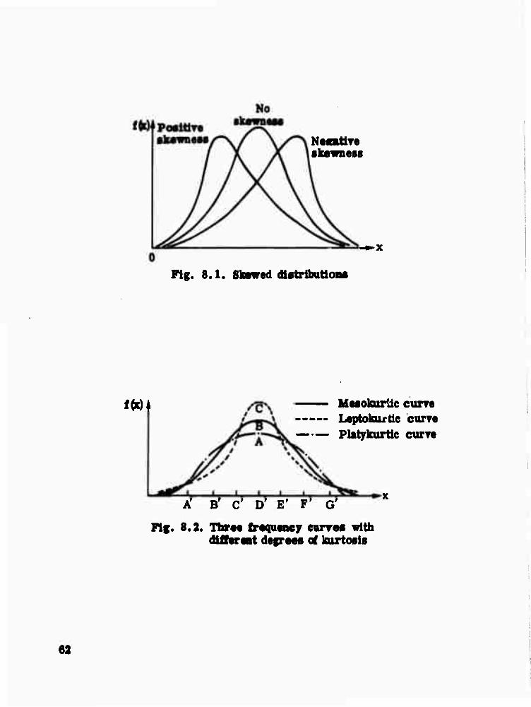
N«nttTe •kewness

»>x

Fig. 8.1. Stowed dtatrlbutton«

f«l — Meiokurüc curre — Laptokuxtic curve Platykurtlc curve

A' B' C' D' E' F' G'

Fig. 8.2. Three frequency eurvee with differ«Bt degrees of kurtosie

62

8.2.2.1 Weibull

The basic three-parameter Weibull distribution has a density given

by:

M-tM'^l-M] , x ^ c

= 0 X< €

where:

f(x) = Weibull probability distribution

f = location parameter

A = scale parameter

n = shape parameter

In most applications the location parameter, c, is known. In

cases where it is not known, it can be estimated from the observations:

c = min[x.] .

(8) Better estimates of c can be obtained using techniques developed by Dubey, ;

however, the improvement is not usually sufficient to warrant the extra

effort involved.

The maximum likelihood estimators for the three-parameter Weibull

distribution result in a set of equations that can be solved by iterative

methods which are very tedious to perform. If the location parameter is

known or estimated, the maximum likelihood equations for X and rj can f51) be solved fairly easilyv ' and are given by:

2yxi ^nXj n

?-" n . ;>xi = 0 (8.1)

§ »i"

63

and

X = (Dtj'/n)1^ (8.2)

where:

TJ ■ Maximum likelihood estimator of rj

X ■ Maximum likelihood estimator of X

Equation 8.1 can be solved by the Newton-Raphson iterative procedure.

1 gj-qP

where: n

S, = 2 ^ xl i=l

sj «g (In x/x^

The estimate f? is biased and should be corrected using the unbiasing fac- A

tors in Table B-lof Appendix B. Then, the estimate for X can be obtained

directly from (8.2). Further improvement can be obtained by using Menon's

estimators.(38)

64

8.2.2.2 Johnson Distributions

As indicated in Table 4.3, there are three Johnson distributions. These

three are generally denoted S., SB, and S.. because these distributions

are related to the normal distribution through a logarithmic transformation

(S.), bounded transformation (SB), and unbounded transformation iS„).

The problem of estimating parameters of the Johnson distribution thus becomes a two-step procedure. First determine which distribution to use, then

estimate the appropriate parameters.

The probability density functions for the three Johnson distributions

are:

SL: fjfr)

SB: f2(x)

Jzn{: -^{-^♦«.(x-ofj ; X2 €

(A

c< x< f+ X

SU: f3(x)

Jto J {*-€)* + X58

exp ..(,.... j(¥).[^..]-"lf -•<x < •

In these distributions TJ and y are shape parameters, X is a scale parameter, and c is a location parameter. These must satisfy:

TJ >0, X>0, -«< y, c < + «

In Section 8.1, expressions are given for the skewness, /L, and

kurtosis, /S,» oi the samPle data. These are used to determine which

65

distribution, S,, SB, or Su to use. This can be accomplished by plotting

the sample ß. and /32 on Fig. 8.3. The location of the sample point 01, /32) indicates the distribution to select. One warning must be given,

however. Figure 8.3 is accurate for categorizing distributions given the

true value of 0. and /S». The values for 0* and 02 derived from the

sample (Section 8.1) are estimates of the true values. Thus if the sample

point falls near the edge of a region in Fig. 8.3, i.e., near the SL line,

then it would be prudent to try all three Johnson distributions or to select

one or more based on possible boundedness of the random variable in ques-

tion. Examining the density functions given above will aid in this

determination.

The parameter estimates for the Johnson distributions are given be-

low. The estimates of the Johnson parameters are not maximum likelihood

estimates, except for the S, (* known) case, however they are the most

practical to use. The approach taken is to use percentile points from the

data. Recall that a 100 a percentile point for the population, xa, is that

value of x for which P[x s xj = a. We assume that the random sample

Xj,...., x has been ordered to give the order statistics W1< ... < W .

Then the kth order statistic will provide an estimate for the 100a percentile of the population, where:

(8.3)

a = k_ n

1 1

This will be required in subsequent application, S. (' known). In this case the estimators for n and y are respectively, t-1/2

V = I£MV<)]2-[I£

i=l

InCXj - c)

i=l

and (8.4)

Att

n

y = -f ^

InCXj - c)

8-

Region for Johnson Su Distribution

J9

2-

Line for student t distribution

Normal Distribution

Line for Johnson S^ Distribution (lognormal)

Region for Johnson S3 Distribution

Impossible Region

f

ßi, SKE^NESS f

Fig. 8.3. Selecting a Johnson Distrit ation from Skewness and Kurtosis

67

Thus, from the sample x.f...fx the parameters 17 and y can be readily A A 1 n

estimated with n and y, respectively.

S, (c unknown)

Again, the maximum likelihood estimators may be obtained but with some

difficulty, and it is perhaps better to use the percentile approach. That is assum«

the percentile points xa , xa , and xa have been estimated. These are

required since there are three parameters *, »j, and y to estimate. If

za is defined as the value of the variable in the normal distribution function corresponding to the cumulative probability a , then.

za3 = y+T] ln(xa3 -c)

Explicit solutions cannot be obtained for €, y , and TJ from these

equations although they can be determined iteratively. However, the following

example will illustrate the use of one simplification.

Suppose a sample size of n = 51 has been obtained. The 6th, 26th, and

46th order statistic from Wj < W« < ... < W51 will be used to estimate the

following percentiles:

^ = x.l = W6

xa2 = x.5 = W26

^3 = x.9 = W46

where aj i = 1,2,3, is obtained using Eq. 8.3. From Table B-2 in Appendix B:

68

z.l = -1.28

z.5 = 0

z.9 - 1.28

From Eq. 8.4:

V = 1 »["fev)] -1

y = rf in

€ = W26-e -y/tJ

The advnntage of selecting a« =1 -a« and a« = «S should be noted.

The percentr jb chosen are, of course, rather arbitrary and, therefore,

many estin utes could be obtained for c, y and 17. In this case, comparisons of . r. «ative goodness-of-fit for each selection may be appropriate.

SB(c,Aknown)

This case implies both end points of the distribution are known. Using

the percentile method, estimators for y and rf may be obtained:

n = z - z «2 «1

In €\f€ + X - X

rX - C\/C + X - X

(8.5)

y = z - T> In X -f

tt2 « + X - x

69

Sg (General Case)

This case implies that none of the parameters are known and requires that the appropriate number of equations of the form

zN = y + 77 In a

x - f a X + c - x a

be solved for the unknown parameters. Generally, this will lead to tran- scendental equations which can be solved numerically. There is one simplification in the case where c is known and the percentiles are selected such thai a =a1 =1 -a» and a« = • 5 (only three equations of the type

A

required for this case). The solution for X for this case is

p. 5- c)(xtt- (Mx ,.- cKx^- 0 ^-«Xx^-,)-] X ' ^ \ (x,-^-(xa-0(^-0 J "•«

Equation 8.5 may then be used to generate estimates for 17 and y since with 8.6 the problem reduces to one with both end points known.

SJJ (General Case)

For general case of the STT system, Johnson has generated tables f22x) that are useful for determining the parameters.v ' These are presented

in Tables B-3 and B-4 of Appendix B. The tables were developed from solutions of equations defining the relationships of the first four moments to the parameters.

Use of the tables first requires that the mean, variance, skewness

and kurtosis be calculated. The values for 7/L and 0« are then U8ed to

obtain the estimates for y and 17 from Tables B-3 and B-4, respectively.

70

The A and c estimators are calculated using:

X= , -____-. „^^ (8>7)

||(w-l)Lc0rtl/i?)4ll \

€ = x + X Jüö sinh (I) (8.8)

where s is the sample standard deviation (see Section 8.1)

To illustrate use of the tables, assume a random sample gave

V^ = • 5 and /L = 6 • From Tables B-3, B-4

y = - .3278 and 77 = 1.672

X and € may now be calculated directly from Eqs. 8.7 and 8.8.

8.2.2.3 Pearson Distributions

There are twelve Pearson distributions. These are generally indicated

by Roman numerals: Type I through Type XII. The problem of estimating

Pearson parameters, like those of the Johnson, becomes a two-step problem.

First determine which Pearson Type to use, then estimate the appropriate

parameters. To determine which Pearson distributions to use, the skewness, 0-,

and kurtosis, ß,» of the sample data (see Section 8.1) are needed. The sample point (0 , /§„) should be plotted on Fig. 8.4. The location of the

sample point indicates what distribution to use. A warning needs to be given

on using this procedure. The point (/L, jL) calculated from the data as in

71

0 0.8

t 6'

0 C 1.8 1 .6 2 4 3 .2 4 .0 4

Skewness ß

.8 5.6 6.

1

4 7 .2 8 .0 8 .8 9 .6 10. i

N,

i.4

R "N^

IMP

"li 1- _ „, 4.d ^ Ns _. — — IV—^

4 ft1 v^5 ^ ^ ^^ \ OSSIBLE

5.6 \ V ̂ 1 .^ S^ ^ AREA

6.4 S A S^ ^ ^

^IX

7.2 \ v >;

J^ i^ K^ L ._

8.0 N

sjv X • ^1 ^"S

8.8 NT lyv V s Xflhs X^

9 6 " N

> ^ \

10.4 i ^ s^

*-«

^ ^J ̂ v N^ tl 2

■ X 1 \7T N V^ ̂

^ V»

r^osis 12.0 02 12.8

13.6

1 \j iV s. N^ ̂

— 1 ^

^

^M ______

>- Vs ^

14.4 \l\ Ix,^ "^ ^ i

^s

15.2 _ — \ N s. \ N ̂ — III _ i—

16 0 ,

V \ \

v % 16.8 i N \

■

17.6 IV \ N 18 4 V N vN

\ s

19.2 \ \

20.0 \ \VI

\ v\ L

'

20 8 i

1 \ \ v :

21 6 v. A \\

22.4 \ \! L

23.2 1 1 \ ^

24.0 \

Fig. 8.4. Selec tion o f Pea rsoni Pypef rom S kewne ss an dKurt tosis

72

Section 8.1 is only an estimate of the true values. Thus if the sample point

falls near a line separating two regions in Fig. 8.4, the Pearson Type in

either region or in the line may fit the data. In this event more than one

Pearson Type should be tried. It should also be clear from examination of

Fig. 8.4 that only Types I, IV, and VI are indicated by regions; therefore,

in practice only these types will be indicated by strict application of this

selection procedure.

Selection of a Pearson Type may also be aided by examining the

Remarks column of Table 8.1. This table lists all twelve Pearson Types and some information on each. The form of the density function should be ob-

tained from Table 8.1.

The parameters for the density functions are given below.

Typel

m1 m« . f(x) = yoH) H) whereR ?) •

Calculate the quantities

r = 6(/S2 - /Jj - l)/(6 + 3^ - 2/32)

t = \ s&J^r + 2)2 + 16(r + 1)]1/2

m. and m« are given by:

1 m = J r - 2 ± r(r + 2) r h ] [^(r + 2)2 + 16(r + 1)J

If fi, is positive, take m« to be the positive root

Sj = t/(m2/m1 + 1)

73

«>

• Q 00 e W 1 ä ä g

•s

•si? 83

h

l«!l ?il^i o a _

fill?

2 e c u 5 c « ■- •s^ = }; e

if

I1 ■

8»,

t? •* ^ >J2

c.

f II

f I II II I 3

a M

§^•8'S

«II S5 Ä

fl

? E

? ♦

►•

'I N If*

f

\X I K0 ►?

«L «u K ►P Ö -O

0

I 1 :•

fe s B > g B B

74

a2 = tAnij/mj + 1)

y« = m1

1 m2 z rCmj + m2 + 2)

o nij + m * ntnij + l)r(m2 + 1) (mj + m2)

Typ611

2'm

f(x) =y0 (l-^

The function parameters are found as follows:

5fl2-9

2 282^2 a = TTjT

v - JL . r(m j. 1.5) yo " ^ ItrnTl)

Type III

f(x) = y0 (1 + x/a)ya e_yx

The function parameters are given by:

75

28l 03 = * 's2

0 a epr(p+l)

Type IV

'(x) = y0 l1 +"2 I exp(-i/tan x


y = 6(^ - ^ -l)/{2ß2-Zß1 -6)

m = |(y + 2)

v =-y (y-2)v'^"Cl6(y-l)-ß1(y-2)2]'1/2

= [i6 (16(y"1)"¥y-2)2)J yo = V[aF(y,w)]

where F(y, t/) is given in Reference 42. TageV

f(x) = yox"p exp(-y/x) (x > 0)


8 + 4 JT+ß* p = 4 ^ !

y = s(p - 2) 1^3)

yn = ^A'Cp - 1)

76

Type VI

q2 ql £(x) = yo(x-a)Zx 1


y - 60^-^ -DAö+Sßj -2ß2)

a ^^{^{y + lf + my+m1/2

q« and -q. are given by:

q =^2±^n2i[ßi/[^(y + 2)2 + 16(y + 1)]]l/2

a 1 z r(ql) yo = rlqj -q2-l)r(q2 + 1)

Type VII rm

'«•yo(>^)


5AJ-9 m = 2ißf3)

- Äj-3

= ^^ rr(m) yo ay^ r[m-0.5]

77

TvoeVIII

f(x) = y0 (1 + x/a)"m


a = ± s (2 - m) 7(3 - m)/(l - m)

yo = (1 - m)/a

where m is the solution of

3,, a . „2 m (4 - /Sj) + mA(9^ - 12) - 24^m + 16^ = 0 0 < m < 1

Type DC

m f(x) = y0(l + x/a)


a = ±s(m + 2) 7m + 3)(m + 1)

yo = (m + l)/a

where m is the solution of

m3^ - 4) + m2(9^1 - 12) + 2imß1 + 16/^ = 0 m >0

TypeX

f(x) = yoexp(-x/s)

The parameter is given by:

y = s

78

Type XI

f(x) = yox -m


yo = hm'1 (m - 1)

b = ±s(m - 2) J{m = 3)/(m - 1)

where m is a solution of

m3(4 - ßj + m2{9ß1 - 12) - 240^ + 16^ = 0

TypeXn

f(x) = v s (V^.y^.x]^3^ s (4 + ßl - Jßj - x

y is given by

where

y0 = r(m + Dltl - m)/b

m = V/Jj/O + ßj)

b = 2s 7(3 + /Sj)

79

9. GOODNESS-OF-FIT TESTS

Goodness-of-fit tests are statistical tests for evaluating whether a

group erf data supports the assumption that the random variable from which

the data are drawn has come from the assumed probability distribution.

These tests are helpful in accepting or rejecting the conclusion that some

random variable follows a tentatively selected probability distribution.

The technique of applying statistical tests of distributional assump-

tions follows three basic steps:

1. A number known as a test Statistic is calculated from the obsenred data.

2. The probability of obtaining the calculated test statistic, assuming the selected distribution is correct, is determined. This can often be done by using precomputed tables of percentiles of the distribution of the test statistic.

3. If the probability of obtaining the calculated test statistic is low, the conclusion is that the assumed distribution does not provide an adequate representation. If the probability associated with the test statistic is not low, then the data provide no evidence that the assumed distribution is inadequate.

It should be clearly understood that although this procedure allows

rejection of a distribution as inadequate, it never proves that the model is

correct. In fact, the outcome of a statistical test depends highly upon the

amount of data available - the more data there are, the better are the chances

of rejecting an inadequate model. If too few data points are available, even

a model that deviates grossly from the assumed model frequently cannot be

established as inadequate.

81

Table 9.1 provides summary information on goodness-of-fit

tests and also indicates on which distributions the tests are applicable.

After a test is selected from this table, instructions on how to perform

the lest can be found in the subsequent sections.

A comment on using goodness-of-fit tests on the complex distributions (Weibull, Johnson, and Pearson) may also be helpful. These dis-

tributions are designed to fit almost any set of data well. It is, therefore,

unlikely that any of them will be rejected by a goodness-of-fit test. Using

goodness of fit tests on any of these distributions will not generally give

the analyst much further information on the form of the true distribution,

and he may elect to accept one of these complex distributions without a

goodness-of-fit test.

This brief background should suffice for practical use of goodness-

of-fit test in simulation modeling. In the following section, a simple selec-

tion procedure is given to determine what goodness-of-fit test to use based

upon the probability distribution tentatively selected to model the random

variable in question. In the following sections these tests are described

and instructions for performing the tests are given. Although there are

numerous statistical tests, these are the most powerful available.

9.1 CHI-SQUARE GOODNESS-OF-FIT TEST

The Chi-square goodness-of-fit test is probably the most widely used

and versatile technique for evaluating distributional assumptions. It can be

applied to test any distributional assumption without having to know the values

of the distribution parameters. Its major drawbacks are its lack of sensitivity

in detecting inadequate models when few observations are available and the

frequent need to arrange the data within arbitrary cells which can affect the outcome of the test.

82

a o

X

S i P.

5

5 I

11 0, Q

ill 11% Uli -"I

Jill

to n o o e

.2 e-n I i £.2 «I

Jlll^l S IB —

1^ = °^

•<

HiS

lea

111 hi ■2 3 5 nub « Si«

> Ü g 0) O 3

ill « u u

I | si

<;3

MM I«

111 .2 ga

||l III

ll MX« ^S gi

ll« HSS

i

4

2 § i 0.2 SfüSTJ

c if.

4>

s 5 _, h «I

z.ZZ£

S LI

41 ill 11] III < x-o

ll B > O V-

s|

S b

ill

c 2 t o - 0

U

si u^

:ÜS

pi i I

I

?g83>

.1 52

11

83

The Chi-square test is used as follows:

Step 1, Estimate each of the unknown parameters of the assumed distribution.

Step 2. Divide the data into k classes or cells and determine the probability of a random value from the assumed model falling within each class. Two methods for this are presented: the first method is applicable if the data arc initially arranged in frequency classes, and the second applies when the data are not initially tabulated in classes.

Method a. The number of cells, k, will be the number of classes of the tabulated data subject to the restriction that the expected number of observations in each cell under the assumed model is at least 5. Let CLj and CUj denote the lower and upper bounds of the ith frequency cell. The distribution of the assumed model (using the estimated parameters) is then used to estimate:

Pr(CL. ^ x < CU.) , i = l,2,...k .

Method b. When the number of observations, n, is large (>200) a good rule is to take k as the integer closest to

k' = 4[0.75(n-t)2]1/5 .

For moderate values of n a good rule is to make k as large as possible but with the restriction k < n/5. The cell boundaries xi,..2> • • «Xj are determined from the cumulative distribution for the assumed model (using the estimated parameters) as the values such that:

Pr(x ^xj) =^,Pr(x ^x2) =|,... Pr(x ^.j) = ^^ .

Step 3. Multiply each of the cell probabilities by the sample size n. This yields the expected number E: of observations for each cell under the assumed model. For Method 2b:

Ej = nA , i = l,2,...k

Step 4. If the data are not initially tabulated, count the number of observed values, m., in each cell. Otherwise, determine m. directly.

84

Step 5. Compute the test statistic

k (m - E )2

2 V^ V i i

i=l 1

For Method 2b this simplifies to

x2 = -i 7 uv. |- n

o Step 6. Compare the computed value x with the tabulated percentiles for a chi-square variate (Table B-5) using k-r-1 dep^ees of freedom, where r i^the number of parameters that were estimated in Step 1. High values of X signify that the observed data contradicts the assumed model. For example, if the above calculated value x exceeds the 0. 95 tabulated value of Chi-square, the chances are less than one in twenty that the data could have come from the assumed distribution.

9.2 KOLMOGOROV-SMIRNOV TEST

This test is used to evalute the assumption that a sample belongs to a

specified known continuous distribution. It is a distribution-free test and is

a good test for small samples. In general, it is a more powerful test than

the Chi-square where it is applicable. Although the test is designed for com-

paring a sample against a specified and known distribution, the test is robust

enough that it may still be applied to distributions whose parameters are

estimated from the sample data. The effect of estimating the parameters of

the distribution from the sample is to reduce the critical level of the d (N)

statistic, i. e., the level erf significance is really higher than the a associated

with the chosen d (N). Hence, if the chosen d (N) statistic value is ft a

85

exceeded in the test, it can be safely concluded that the discrepancy is

significant. Grouping observations into intervals also tends to lower the

value of d. For grouped data, therefore, the appropriate significance

levels for testing should be chosen smaller than the significance levels used

for a complete sample.

The test is used as follows:

Step 1. Rearrange the sample of size n to obtain the ordered sample x^, x0,... x where x1 ^ x« ^.... s x . 1 z n l c n

Step 2. The sample cumulative distribution then takes on values oi 1/rt, 2/n,...., n/n at the points x., x .

Step 3. Calculate the cumulative frequency values for the assumed distribution at the sample values of x1, x0, ... x .

Step 4. Determine the maximum deviation, d, between the sample cumulative distribution and assumed cumulative distribution from Steps 2 and 3.

Step 5. Compare the calculated deviation d with the test statistic d (n^ found from Table B-6 for the desired level of significance. If d exceeds the value d (n) then the assumption that the sample comes from the assumed di^fribution may be rejected at the lOOoro significance level.

9. 3 W-TEST

This test is used to evalute the assumption that a sample has a normal [

distribution. It can be used to test the assumption that a sample fits log-

normal distribution by using the log of the sample values. The W-test has

been shown to be an effective technique for evaluating the assumption of

normality against a wide spectrum of non-normal alternatives, even if only

a relatively small number of observations are: available. It is generally 2 more powerful than the x > especially for small sample sizes.

The W-test is used as follows:

Step 1. Rearrange the sample to obtain the ordered sample x. ,x9. where x1 * x0 *... ,x . 12 n

86

n'

Step 2. Compute

1=1 1=1

.y n

where x is the data mean.

Step 3. If n is even, set k = n/2; if n is odd, set k = (n-l)/.2. Then compute.

b = 7 a . ..(x ., - x.) , tmj n-i+1 n-i+1 r ' i=l

where the values of Zji-i+i for i = 1,... .k are given in Table B-7 for n = 3,..., 50. Note that when n is odd x . does not enter into this computation.

Setp 4. Compute the test statistic

W = b2/S2 .

Step 5. Compare the calculated value of W with the percentiles of the distribution of this test statistic shown in Table B-8. This table gives the minimum values of W that we would obtain with 1,2,5,10, and 50 percent probability as a function of n, if the data actually came from a normal distribution. If the percentile is lower than the selected level of significance, then the hypothesis of normality can be rejected and accepted otherwise.

9.4 WE-TEST

This test is used to evaluate the assumption that a sample has an ex-

ponential distribution with the origin unknown. Percentiles of the WE dis-

tribution have not yet been tabulated for sample sizes other than 7 to 35.

The comments on the W-test are also applicable here.

87

The WE-test is used as follows:

Step 1. Calculate the test statistic:

(x-x.) WE

i=l i=l \ i-1 I1

where x^, 1= 1,... n, are the n observed values, x is the smallest value, and x is the data mean.

Step 2. Compare the computed value WE with the 95 percent and 90 percent ranges given in Table B-9. This test is two-sided in that too-low or too- high values indicate non-exponentiality. Thus, if the computed WE value falls outside the 95 or 90 percent range, then the chances arp less than one m- 20 or one in 10, respectively, that the observed sample was drawn from an exponential distribution.

9.5 WE0-TEST

This test is used to evaluate the assumption that a sample has an expo-

nential distribution with the origin c known. However, percentiles of the distri-

bution WE have not been tabulated for sample sizes other than 7 to 35. The o * comments on the W-test are also applicable here.

The WE -test is used as follows: o

Step 1. Subtract the known location c from each of the sample values x..

Step 2. Calculate the test statistic

88

where x.f 1 = 1,..., n, are the n sample values and x is the sample mean.

Step 3. Determine whether the computed value WE lies outside the tabulated 95 percent and 90 percent ranges shown in Table B-IO as a function of n. This test is two-sided in that too-low or too-high values indicate non-exponentiality. Thus, if the computed value of WE0 falls outside the 95 percent range, the chances are less than one in twenty that the observed sample was drawn from an exponential distribution with the assumed origin.

89

APPENDIX A

COMPLEX PARAMETRIC DISTRIBUTIONS

91


A. 1 INTRODUCTION

Although the reader probably has a good general knowledge

of the simple parametric distributions, he is likely to be unfamiliar

with the complex parametric distributions. The main text of this

volume indicates when and how to use these distributions, but all with-

out requiring a thorough understanding of the complex distributions.

This appendix is intended to give the reader some background informa-

tion on the complex distributions so that he will be better able to under-

stand and use the related material in the main text.

93


A. 2 WEIBULL DISTRIBUTION

The Weibull distribution is best known for its application to reliability

analysis where it is known to fit a large class of life (time to failure) dis-

tributions (53). The basic distribution suggested by Weibull is to define

(p(x), where the cumulative distribution function F is given by

F(x) = P[X< x] = l-e"^^ = JX f(x)dx . -00

One of the simplest forms for (p(x) is

<p(x) = ÖE^ x ^ c

= 0 X< €

in which case

F(x) = 1 - e X x 2 c

= 0 x< c

and

. (x-c)^

f(x) = t?/X(x-€)T7'1e ^^ x^c

= 0 X^ €

The parameter c is called the location parameter in the sense that it

defines the lower limit for the random variable x. For the special case

where f = 0,

f(x) = n/xxn V*

95


and

F(x) = l-e'x /X .

The values of n and X may be selected to provide a large number of shapes some of which are sketched below in Fig. A. 1. For this reason TJ is called a shape parameter and X is called a scale parameter since it scales the value of x.

*~ x

Fig. A. 1. Weibull Distribution lor Various Values of Parameter 77

96

It should be noted from Fig. A. 1 that rj1 ss 1/2 might represent the shape parameter for the early failure region and no = 3 the shape parameter for the wear-out region in a typical reliability application.

■■

97

A. 8 JOHNSON DISTRIBUTIONS

These distributions were proposed by Johnson who used trans- formations of the normalized normal random variable to generate empirical distributions^!^). The main advantages of this approach are that percentiles of the empirical distribution may be obtained using a table of the normal probability distribution, as will become apparent later, and that the approach encompasses a broad class of problems.

To introduce the Johnson distributions, assume that it is desired to obtain a probability density function for the random variable X about which little or no information is available. Then, a general transformation from X to Z is postulated, where Z is a normalized normal random variable, as follows

Z = y + T?T(X) ,

where yand TJ and parameters to be determined.

In most situations, the transformation T(X) will be unknown. However, Johnson proposed three families of distributions, referred to as the S., SB, and S» systems, respectively, defined as follows

SL(Log-normal)r(x) = in (x-c)

SB(Bounded) T(x) = lntj~~~>

SydJnbounded) T(x) = sinh"1^)

The undefined regions for x above imply T(x) ■ 0.

€< X < C + X

-"< X <•

99


Similar to the Weibull distribution, tj and y are shape parameters, X is a scale parameter, and c plays the role of location parameter which shifts the region of relevancy for x. These parameters are subject to the following constraints:

tj>0 ; X >0

-• < y < •

In some cases, these parameters may be identified from a basic understanding of the process. For example, if the random variable x must be non-negative, then e = 0 and the S., or lognormal distribution, might be appropriate. If x is restricted to a finite region, c< x < c +X, then S» (bounded distribution) may be appropriate. An infinite range for x would suggest the S„ (unbounded) distribution.

The probability density function for the distributions are as follows:

.2 SB: f2(x) . J.

exp ■H'-fw-^-n)! -•<x< •

100

The density function for the S. system is a three-parameter distribution commonly called the log-normal distribution. This is known to describe many familiar events such as amount of inheritance, income, particle size from breakage, etc.

As previously mentioned, the class of situations encompassed within these distributions is large. An indication of the flexibility in defining a large number of shapes is evidenced in Figs. A. 2 to A. 4 which illustrate several forms of the S. , S- and Su density functions.

The difference between the three types of Johnson distributions can be characterized by the relationship between the distribution skewness and distribution kurtosis. Section 8 of this volume contains a discussion of skewness and kurtosis; however, a summary definition is that

&l=u$/a (skewness)

and

62 ' Hi* (^rtosis)

To help in the definition of the relative variation in 0* and /J«. Johnson prepared the results as shown in Fig. A. 5. Note that the lognormal distribution is defined by a line given by:

/Jj = (w-1) ((o+2)2 ; > 0 4 3 2 02:=<ti+2(«)+3(o-3 ; > 0

where

is the shape parameter for S. .

101

m i

Y "0; i?«l

•- X

Fig. A. 2. Johnson Probability Density Functions for S. (c = 0) Li

102

y K 0; i; - 0.5

y-0.533 »j »0.5 y •» 0; rj « 2

y-i: n-i

3.5

3.0 A y«i

2.5 / \

2.0 " / \

1.5 ■ / \

1.0- / \

0.5- 7 V 0- / >-

Fig. A. 3. Johnson Probability Density Functions for Sn («= 0 ; A= 1) B

103

Fig. A. 4. Johnson Probability Density Functions for S..

104

8T

M «X

Region for Johnson Su Distribution

Line for student t distribution

Normal Distribution

"(

Extension according to

ßt - (w-1) (« + 2)2

/5a.<l)4+2«s + 3w,-3

Line for Johnson S^ Distribution (lognormal)

Region for Johnson Sg Distribution

Impossible Region

(ß*~ßx <1)

01, SKBWNBSS

Fig. A. 5.. Regions of Definition for Johnson Distributions Based on Skewness and Kurtosis

105

It should be recognised that estimates for/J - and fi- may lead to a wrong conclusion as to the type of distribution to be used. The confidence that this will not occur is related to the accuracy of the estimates. In ease of doubt, a goodness-of-fit test may be used to help in a decision.

106

y

A. 4 PEARSON DISTRIBUTIONS

A general claf s of probability density functions known as the Pearson family" ' ' , is given by solutions of the differential equation:

% b0+blX+b2X

The solutions of this equation were classified by Pearson into twelve families of curves shewn in Table 8.1. These curves are displayed in Fig. A. 6. The Pearson distributions are related to the standard densities frequently discussed. For example: the gamma distributions are Pearson's Type HI curves, the normal is a Type VII, the beta is a Type I while the beta with parameters a = 8 is represented by the Pearson Type U curves.

This system of density functions is very appealing from the standpoint of fitting sample data, the reason being that only the first four moments need be calculated. Pearson's methods of fitting sample data consists of the following steps:

1. Compute the first four moments, n-, ji«» U3» u4 of the sample data.

2. Calculate the numerical value of the parameters 0* andjS*» where:

/J- = skewness,

|5 2 = kurtosis.

107

TYPE I

TYPEH

in« m,

'»-M1+q) C-q)

2 m

TYPE in ifW

-a o

TYPE V

w = yo(1+f) e va -yx

f«=y-pe-y/x

TYPE VI

fW q2 ql

-a

Fig. A.6. Typical shapes of Pearson distributions (Sheet 1 of 2)

108

TYPE vm f«

x=-a o

TYPE IX

x=-a

1«

f«s3r0(l + |) -m

'«=yo(1+ir

TYPEX

f(x) = yoe -x/a

TYPE XI «w f«=y0x -m

TYPE XII f(x) = y>(^J » ^Vy^TTJ

Kote: Type IV and vn appear as normal distributions.

Fig. A.6. Typical shapes of Pearson distributions (Sheet 2 of 2)

100

Skewness ß*

0 o.a

0 0.8 1 .6 2 .4 3 .2 4.0 4 .8 S .6 6. 4 7 .2 8 .0 8 .8 9.6

II—l^r t 6 N, t.4 ̂ \, n-tl ZN ̂ v ̂ 1

•«» 4.0 \ ̂ ^ \ • IMPOSSIBLE

4.81

5.6 .N x*1 aN^ N., | REGION •

\ V V. $53 x^ v. 6.4

N A ^ v_ ^ -IX

7.2 \ Vi ̂ v "^ i^ ̂ K

8.0 \ vs ^ v ^s « ̂ <^! V.

8.8 \ Vv \ 'S C5 1 1 ̂ w

9.6 10.4

>

Vv >

^. jofcs X ^S N. ^ v Ns V?* *% Sfai

■^ v. 11 2 \ v.N \Nl s«f^. ^■R V ^

Kurtosfs 12.0 ß2 12.8

13.6

\ V N^ ff .

V

^ "s. 1

\ \ ^ k*»

V ^ s.

V \ V I "\

14.4 \ \ Xl-ik ^

V (J Shaped) s

15.2 0s s \ N ̂ — m

16 0 \ \ \ N 16.8 \ s s. \ VI ' V 17.6 IV

i

V \ \ \

18 4 HE ITEROTYP] [C \ N

V S 19.2

AR EA , \ \ \

20.0 \ V^

A \\

20 8 \ \ \

21.6 22.4

v. A \\ \ \N k

23.2 v \

24.0 \

Fig. A. 7. Types of Skew Frequency for Values of ß. and for the Pearson System 1

110

These parameters determine the type of Pearson distribution which appropriately matches the sample data.

3. Equate the observed (sample) moments to the moments of the appropriate distribution expressed in terms of its parameters, and

4. Solve the resulting equations for those parameters thereby completely specifying the distribution function.

The relationships between ß* and jS* for a given Pearson distribution have been represented in a convenient graphical form in the so-called /L, /Sg- plane shown in Fig. A. 7. The normal distribution corresponds to the point

0i = 0> 09 = 3 in the ^V^2 ^Bne' TyPe ni distributions are to be chosen when the point ßl,ß2 is on the line 2ß2-3ßl-6 = 0 and Type Vwhen (ß^,ß^

is on the cubic

Bfa + 3)2 = 4(4fl2 - ZßJ {2l>2 - 3^ - 6).

In considering the subtypes under Type I, a biquadratic in 0- and 0« separates the area of the J-shaped curves from the regions of limited range modal curves and the region of the U-shaped curves.

In summary, the curves traced in the (flL,^ J- plane provide a means of selecting the Pearson distribution appropriate to a given collec- tion of sample data. For further details and numerical examples see Elderton(lO) and Kendall(27).

Ill

APPENDIX B

PROBABILITY TABLES

Preceding page llmk 113

/ s

TABLE B-l Unbiasing Factors for the M. L. E. of ty

n S C 7 I > 10 11 12 13 14 IS 1C

B(n) .66» .752 .792 .120 .M2 .8S9 .t72 .883 .893 .901 .908 .914

II 18 20 22 24 2« 28 .tO 12 34 36 38 40

B(n) .923 .931 .938 .943 .947 .»SI .»SS .958 960 .962 .964 .966

n 47 «4 4» 48 50 S2 S4 Sfi 5fl 60 62 64

B(n) .968 .970 .971 .972 .973 .974 .975 .»7« .977 .978 .979 .980

n 66 68 70 72 74 76 78 Dn 8S 90 100 120

*(n) .980 .981 .981 .982 .982 .983 .983 .984 .985 .986 .987 .990

115

Preceding me blink

TABLE B-2

Percentiles of the Normal Distribution

F(x)=JX 7ke -t2/2

-/SF dt

m .00 .01 .02 .03 .04 .03 .00 .07 .OS .09

.0 .5000 .5040 .5080 .5120 .5100 .6190 .5239 .5279 .5319 .5359

.1 .5308 .5I3S .5478 .5517 .5557 .5596 .5636 .5675 .5714 .6753

.3 .5793 .5832 .5X71 .5910 .5948 .5087 .1)026 .0001 .«103 .0141

.S .6170 .0217 .6255 .C2t)3 .6331 .6368 .0406 .0143 .«ISO .6517

.4 .0551 .6591 .6628 .GOU4 .6700 .6736 .0772 .6808 .6344 .6879

.5 .0015 .0050 .6985 .7010 .7054 .7088 .7123 .7157 .7100 .7224

.« .7257 .7291 ".7321 .7357 .7380 .7422 .7151 .7486 .7517 .7519

.7 .7580 .7611 .7642 .7673 ,7704 .7734 .7701 .7701 .7823 .7852 4 .7881 .7910 .7930 .7967 .7995 .8023 .8051 .8078 .8106 .8133 .9 .8159 .8186 .8212 .8238 .8204 .8280 .8316 .8340 .8305 .8389

1.0 .8113 .8138 .8461 .8-185 .8508 .8531 .8554 .8577 .8599 .8621 1.1 ,8613 .8065 .8686 .8708 .8720 .8749 .8770 .8700 .SS10 .8830 J.3 .8819 .8809 .8888 .8007 .8925 .8044 .8062 .SOSO .8997 .9015 l.S .0032 .9049 .000« .0082 .0099 .0115 .0)31 .0147 .9102 .0177 1.4 .9192 .9207 .9222 .0236 .9251 .0205 .0*279 .0202 .9306 .0310

1.5 .0332 .0315 .9357 .0370 .0382 .0304 .9100 .0418 .0429 .0441 i.e .0152 .9 «63 .0474 .9181 .9405 .0505 .0315 .9525 .0535 .0545 1.7 .0554 .9564 .9573 .9582 .0501 .0500 .0008 .0610 .0625 .0633 1.8 .0641 .0610 .0656 .0064 .0671 .9878 .vem .OOO.'l .0690 .0700 1.0 .9713 .0719 .0726 .9732 .0738 .0744 .0750 .0750 .9761 .9767

3.0 .9772 .0778 .0781 .078« .9703 .0708 .0803 .9808 .0812 .0817 3.1 .0821 .0826 .0830 .9S34 .0838 .0842 .9846 .0850 .0854 .0867 3.3 .0801 .9864 .OS»» .9871 .0375 .0878 .0881 .9884 .9S87 .0800 3.S .9893 .0890 .0W»8 .<)«K)1 .0901 .0006 .0000 .SOU .9013 .9016 3.4 .9018 .0920 .9922 .oota .9927 .0029 .0031 .0932 .0034 .9030

3.8 .0038 .0910 .0941 .0013 .9045 .9016 .0048 .9049 .9951 .0053 3.8 .9053 .0955 .0956 .0057 .0050 .9000 .9001 .0902 .0063 .0904 3.7 .0905 .0066 .9067 .1X108 .0069 .0070 .0071 .0072 .00/« .0974 3.8 .0074 .9975 .0976 .0077 .9977 .0078 .0070 .0970 .0080 .9981 3.0 .9981 .0982 .9082 .0083 .0081 .0081 .0085 .0085 .0080 .0986

8.0 .0087 .0987 .0087 .908.8 .9088 , .9989 .0980 .0080 .9990 .9900 3.1 .0000 .0991 .0091 .0091 .0092 .9002 .0002 .000-' .C903 .0093 8.3 .9993 .0903 .9994 .9091 .0094 .9004 .0904 .9005 .00011 .0005 3.3 .0905 .0905 .9005 .9096 .0990 .0006 .0900 .000« .0000 .9007 3.4 .9907 .0097 .0997 .9007 .9997 .0007 .0007 .0007 .0997 .0008

a 1.282 1.045 1.060 2.320 3.576 3.090 3.291 3.S01 4.417

^e) .00 .05 .975 .00 .095 .009 .9995 .CÖ005 .ooooo;»

«i -rw] .30 .10 .05 .02 .01 .002 .001 .0001 .00001

(From A. M. Mood, Introduction to the Theory of Statistics. McGraw-Hill, 1950.) — '

116

TABLE B-3

Tables to Facilitate Fitting Johnson Sv Distribution*

Values of —y

1 •ttl» •ITM •Ittl

0-I1M •10M •MM

•074» M

4-1 4-a 4S 44 4»

4T 4t

■•I 0-OXM »a -0374 53 •(«•!

•CMJ

•06lt

0-0491

■0444 •04t4

»•: 61

»■• »•7 SB M

»•I *■] 43 4-4 45

4-7 44 4* 74

71 M 7« 7-4 7»

74

74* 74

»a • 4 •4 • 8

«•a

•034S •0317

003« 0314 •0307 om 0200

oossa •05176 •0S69 •02M ■0357

00151 ■0346 ■0341 •0S3S •0332

00337 •0333 •0*19 0316 4313

0-0106 4306 •0903 4IM 4196

00190 •01H» •01M) •0175 4171

414

0-7373

-3620 •3904

0-3435 •3103 •1953 •1441 •IMT

0)391 •1374 ■UM •lilt •1044

•4ft'« -oo»a >0R«1 ■Oij,:« ■01(14

00.83 •075? •07! ü •Oil»'' ■o«;t.

C . •1 j." '■ ■usui» OAK)

00;.flS •0&!.3 0540 •0'.;7 •0515

0-0804 •04t:» -04 K3 •M73 •0464

00435 0447

-0439 0431 4434

00417 -0410 ■0404 03«*

■0393

003M 0370 0300

-0351 -0343

»M

1-33« 0-7747

•••174

•364* •t*M

»SIM •IMS •1606 •14M •I5M

frl4M •1431 -IS53 •I3M •1334

OHM -113» •1ÜM -1057 -lOSS

o-o;«» -0V".8 •0V30 wm MM

00(156 ■0ti36 ■0ftl4 -0;95 •0777

0-0760 •0743 4:3» -071? 4«M

0-0686 M7S 4MI 4460 44M

0043» 4614 4«M

»M •IS

1-940 IMS O-SIM 4394

M90

00573 0557

•0543 •0539 4514

■44K7 •3931 •3490 •3150

0-3676 ■3647 •MM •SSM •8153

0-3031 •ISM •ISM •1743 •I6M

01607 ■1534 •1477 ■1424 •1*76

n<l3M ■»2W •I3M •1316 •11*3

Ollfil •1121 ■10(14 •1067 •1043

a 1020 •099H ■0977 •0957 •0938

0032O •0PO3 •Ort87 ■0871 01.66

00843 0839

■0HI6 0802

■0790

00747 014«

■0725 ■0707 ■0484

31*9 1-656 1-133 0M30

■5907 •513* ■4(134 ■4074

O3707 ■3404 31*1

■3937 •37*3

0-2S02 ■2451 •2327 ■2216 •3117

0-202-; ■IMO •1872 •1H04 ■1742

01*84 ■1631 ■IW1. ■1531. •14*3

0I45& ■1415 ■I 380 ■1347 ■1315

omn ■126« ■1231 ■I:CK» •1162

01159 ■1137 •me ■109(1 •1677

0-1059 ■1042 ■1025 ■1009 ■0993

00*44 ■0937 •0912 ■Odltr' ■08*6

430

43** ••477 1M9 Ma

0-9116 •7*8« •Ml* •6723 4113

04029 •4234 •SUV •3932 •9306

0 319? •3014 -3857 •2717 •3592

0 24 DO •:':i78 •23SS •im •3123

020« -I9KG •l*2t. • isr.N •191ft

o-m« •1719 •I67K •1*98 •1596

0 1 (WO • 1*26 •1492 •1461 •1432

01404 •1377 •13i2 •1327 ■1304

o-mi •1360 •1340 •1220 •1201

0115* •1132 •ll«l •1073 •I04C

0*5

»-334 1-446

1IS7 OM*l

41*7 •7177 ■4304

08673 •61 (16 •474) ■4397 ■4100

03844 ■M22 ■342« •3254 304»

03961 -2836 •27?3 -«no •K2(

0243H -23fiS ■■mx int.

•3161

03091 •3035 •1983 ■1933 ■1*87

0-1(43 ■1802 -1753 •1725 •16*0

0165« •1624 •1594 •15*5 •1537

O-IS10 •148* •14*0 •1437 -1414

0-1371 •1333 -1295 •1261 •1339

01199 •1171

4 49

3 484 SIM

1 665 1 238 1038 0S8I4

•7733

0 6902 •4343 ■0708 ■5266 •4H91

04564 4'.'KH 4Ü)H

•1836 ■3648

0 3479 •:.738 •SIV! ■31 .1» ■n**

or"«« ■•.•>(.:

.-■MS

■»W4

02433 -S.360 rsoi

■81«"

«•«IS« ?o:.H

-?043 -1V90 •1M1

0-191« ■ 1KN0 •I84> •1810 •177V

0174« •1716 <ICN7 ■1660 ■1633

O-KM •1537 •1494 •1454 •1417

0-1382 ■134«

• a

8139 1414 1-302 I •096 O-9470

0 0363 •750* 4814 4361 -6780

063ht •5010 474*

-44H4 -4254

04050 •JM56 -ssrn

-»411

or.2'c •sn.;

•:tu7 •?tl7»

0 'I'-'H« ••::nz •26.! 3 •2574 ■3509

0-2448 ■2391 ■2337 ■*?8C •2SS7

0 5190 ■2147 ■3105 ■loos ■2027

0 1991 •1966 •1922 ■1891 ■186U

01 so: •1749 •ir.M • It'.3 •1410

0 1670 •1532

•M

3-167 8-IBS 1467 1 378 1-149

1016 0 903!

■8i:'7 •7407 4» II

06311 •ASK« MfO

■i>-yt. ■4J'2£

0-4074 •4453 ■Viib •4076 •3913

0-Ä7 ■'. •iZ..<i •3M.4 •3''. '.

O-U -3.1 •3".> .{<.■

-2ts4

o-rm -27.i. •;'r4B ■W.t.6 ■2M<i

02476 -2426 -7377 -2331 -2tH;

••SMO ■2i>0« -2167 2131

•8095

O-'Ci.'O -1W6K •iwr.! -IP.V» -IBIO

• 1144 -1721

8 I

117

TABLE B-3 (continued)

Values of — y (continued)

WK

4-1 4-3 4-»

4-7 44 4«

f-l

»» ••4 • »

5-« 57 68

6-1 43 *3 64 6-5

6-6 4-7 <>• 6-9 70

7 1 7-2 7» 7-4 7-5

7-* 7-7 ?•■ 7»

SI 63 B» • 4 M •-4 • 7 • S 8«

»■2 ♦ 4 •4 M

10«

OS«

l-TU 1440

IWI 10»« «■0748

•8802 •8038

»7800

MIO «017 ••478

«•6874 •610« «M8 W6J

•4468

0-4283 •41 SS •1S78 •3840 •8714

0-3698 •3401 ■3390 •3207 •320»

0-3IS3 -3046 297.1

-2904 ■3939

02778 -3719 ■2864 -2611 •2681

02813 •3407 •2423 •2381 •2841

0S303 •226« •2230 •210« •2I«3

02132 -2101 -2072 £044

-201«

0-1964 •1916

3363 2-42« 1-90«

1877 134» 1-182 1064 •-»687

0-870« «034

•7461 -6948 -063«

06170 •6646 •666« •6208 •600«

04SS« -4668 •4491 ■4331 •41*4

0-4048 ■3923 ■380« ■3897 ■3698

03600 ■3410 ■332« ■3247 ■3178

03101 •3034 -29«7 -2907 -2849

0-579» •2742 -2692 -2646 •2600

0-266« -2614 -2473 -}436 2397

03362 -2327 •2294 -2362 •2231

02172 -2117

2621

to* 1-70« 1-460 1-280 urn 1-033 0-9484 •»«9» -8083 -7660

0-7092 6693

-4341 •028 -6748

0649* -6270 -6043 -4(176 -4701

04642 -4396 4268 4131

-4013

03»O3 -3799 -370!!: 3611

-36X4

0-3443 -3366 -3293 -3224 -Sit»

0 309»; -3037 -2»M> -292« •2871

0-2822 •2774 •272» •2666 ■2643

0 2603 •2664 •2626 -2490 -24 6f

>23H» •2328

«7«

410«

28M 2-264 1860 1-66» 1392

1-340 I 121 1-024 0-9428

•8781

08184 •7687 -7262 -686» •6630

00226 •«•03 •670« ■6481 •627»

0-60RR -4916 -4768 -4607 -4470

0-4341 ■4221 -410» -<nc4 -S«I8

0-3812 -3723 •3640 •3661 •348«

0-3416 •3347 -328J -3221 •3I«3

»3100 •3063 •3001 •2962 •29Ü4

•-»86» •2812 •2770 -2730 •26ft

••2617 •»84» -2483 •2428 »366

»71

1-622 1-363 1 221 1114 1426

09609 •8877 •6331 •786« •741»

0-7067 613S

•«437 «168

•»»24

0-6700 •649« •6308 •6134 •4973

• 4K24 •46H4 •4664 -4433 -4318

0 4211 -4110 •4014

-3H38

03767 •Sf.:0 -3(Mi7 •3(137 •3470

0-34(17 •3346 •3283 -3232 •3179

03127 -307« •3031 -29)15 •.•941

0 288H -277R •8708 -::oj9 •1676

• M

1931 I «70 I-4K6 I 333 1 216

1117 H04 09042

•039 •8616

0«»S6 •7«47 •7284 •6942 •••03

o-esxo ••162 -5(129 •«734 •6{.:i&

O-saro •1>I0V •6046 •41-U •4772

MS • 99 • •s : IK

2-602 2167 1864 1«4I l-4«9

I'US 1-S21 1-128 l-OM 0-0826

09243 -h-.3» ■KM -7NSI -7621

0 7197 •«•.•04 •6637 -6392 «160

i t)!<'>:\: 6770

-OSCJ -6427 -6:73

4029 303« 2473 2-100 1-M2

I •29 1-470 1342 1-236 1-147

1-071 1-006 0 9485

-8082 •MS«

0-813« -77«« •7460 -71(11 •fli.92

OfiiUfi 04lt>

-C2U^ •ili.-l -6836

0-4C48 | Or.nO . 0 666« •4681 I 4996 I -6603 ■44/1 AHM I ■6302 ■4318 -474« I •i>t24 •4220 "tOJO I -6094

04127 •4039 -3950 •3870 •3801

03729 -30«0 -3.'>W4 3531 3471

03413 •3?.5« •SMf. -32S3 ■32«>4

0 3111 •30'J.'. •2044 •2KI.H •271'K

04530 •4<?9 •4S34 •42'i4 -4168

0<'I76 :>!)9« 3923

•»8W •3784

0 3719 -3667 3497

•3630 •3484

0330«) •32113 311)3 3101'

■3030

04972 ■4H67 -4747 -4044 454«

»407

»071 11-26 I 036 1-484 1-361

1269 1-172 I09H 1033 OP766

01)263 t.820 841:0

•I».i0 7733

OT.M VIO«

-tii)14

-0470

•••S7» 6087

-:.'J16 •6764 '6J>n3

064ft:i -6i:*8 -.'.?C3 -5084 ■4971

0-446,2 ' 0 «Cei -4364 -4279 -4199 •4122

04048 -307« -3910 -3845 3783

-1703 •4607 •4:.76 -l-tf."

0 4406 -«•.•r. •4?'.H ■417,'. ■UM

U 3A«6 | 0 3(,74 -3658 | -31.5;' 3447 -3739

■33n3 -3631 •3276 -3637

3638

»832 2380 2072 1839 I «67

1 610 I I 390 ' 1-28C

1-203 1-129

10«» I 1008 I 0 9481

913'.' «739

0 83«t ROSS

-7730 7463

•1186. I

0 6962 -6744 -6541 -635» -6176

0C0I0 -5866 -6709 6671

-644»

06309 •5203 •Mm -4087 -4888

0 4793 ■4702 -461« -4533 -4464

«4306 •41 «9 -404» 3928

•381«

118

TABU B-3 (continued)

Vahtes of—y {continued)

»A tm IM IM l-M IM IM IM 148 I4S IM

M »4M 8-848 M t4N t-874

M 1471 8481 §•7 14« 814» M 1447 1481 •4M 8M* M MM 1-741 IM4 8184 M 1487 1-884 14« MM

M 1441 1478 1*08 «4M • a 11« 1-871 14*4 847* «4M 8-110 M 11« 1-8« 1*81 14M «4« 871« M 1444 1410 1487 1-719 Mtt «4M M •4«! 1-148 1M7 14« 18M «•8M

M 04477 1088 148* 14« 1417 «438 »-7 4084 1038 MM 1-8M 147t «IM M 48*4 04867 MM 1418 14« 1424 «-6M S-M» «4 •8988 44M 1478 144« 14*4 177» «46» ««13 *<• •8048 ••068 l-OH MM 1»7* MM «4*8 «7M

11 0-7788 0-870* 0*840 MS4 1308 1444 14M ••4M ra •78« -SSM 4444 1414 1237 M62 1-76« «-•17 7S •7268 40*3 •088 1488 1178 1373 14M «029 T-4 •7084 -7823 •8763 04071 MM 1-301 1-637 1-878 S-4M »MC Tf 48U -7873 -B4M -84*6 1077 1438 1-4M 1-748 «-«0« 3088

7-6 00430 0-73,l 0417* 0-8181 14M 1-182 1-874 I0M «4>4 2706 77 •8448 •718« •7810 -8884 ••»46 1-132 1-807 1840 1-877 «•43« 7* «2711 4*?4 -70» -8M8 •804 MM 124» 1-457 1-78« 2411 7«" 4117 473« -7448 •8878 4MI 1044 1 19« 1434 I-84C «437 Kb 6947 •8568 -78M MM 4M» 1008 1-148 1419 1664 1-MS

• 1 048» 04*.W »7040 077M 08M1 0-870« 1-OM 1-260 147« 1-77« 8-2 6C80 4^7 4887 -76*8 8387 43t.3 1-OM 1-207 1401 146V • » •SMS •um» •8*U 7884 41« -90fiJ l-OTO 1-16* 1437 147« 8< 4*48 •«»so 4821 ■717« -7*M -8806 0-88M Ml* 1479 l«80 «5 •8388 •6618 ■6i«8 »Ml -77« •8848 4M8 1076 14«7 142»

W, 0-bStO OSOM M2M MSM 0-7807 0-8304 0424« 1-03* MM 13«1 ••7 •609* •6r.74 •80M 4MI -7818 -8078 •«n 1-004 MM 1404 • 8 •6018 •6481 •6*M •MIO •7140 •78M -•718 0-972» 14« 1482 M •4*24 -8384 •6831 •8SM ■887« -7867 -M77 •943« 1-OM 1-204 • 0 •4884 -8881 4714 4«M M1S -7460 -8M« ■»IM 1426 1-181

9-1 04748 04184 0-6801 M101 «•<M8 07303 0-8048 049M 04948 11«» »■» •4888 -8000 6494 •8078 48M •713» •7818 -80« -M81 1084 «a •4887 -4071 -6398 •BMI 43M 4077 •7CM 444i -M77 1480 M •4811 ■4886 •8888 4748 42M 4*27 •74M 4334 418« 1-019 «•S •4488 -4803 480« •8*4« »IM -80M •781« •8038 M8« 04892

94 043« 0-4784 0-8118 08*40 0-M18 0464* 0-7164 0-7848 08M7 0-M18 ••7 «30« •4048 •8037 •844« -88M -S4M -7003 -7871 •M48 9359 M •4887 4878 4*46 ■634» 47W 4297 •M40 -7603 ■8246 4117 M •4178 •480* MM ■6200 4«M »IfiO -67114 -734« ■MOM -88M IM •4118 •4438 47*0 4174 »687 •8M7 -0694 -719« -7877 -M7S

IM 0-4001 04811 0 4448 0601» 06418 0-8M7 04362 04910 0-7848 0-8280 l»4 •SKM •4IM •4818 4M« »248 4«M 4131 «««4 -7847 -7827 1*4 47M •4088 •4M* •4723 «OM -»4M -8927 ■0420 4978 •7»M IM •8708 ■3978 4878 '4893 4940 4320 -6738 42V8 ■87«7 -7318 IM •8418 •3681 •41« •4478 •4804 -8187 66«« «007 •MM -70M

na »8838 0478* 0-40*S OUM »■4»7» O6028 08404 048«« MSM O-Mll IM 3466 •3703 •3*68 •4M« •4M* 4881 -8864 -M8S -8098 WS» IM — ■6496 4918 -•3(13 114 — mm — _ mm «_ •8M7 -6748 41»« r -^ •"■ "~ — — "" — -6209 -5393 ■Ml»

119

^

TABLE B-8 (eonünued)

Values of-f (continued)

y 14» I4S 14« 14» in 14* 1«) 14» 14» 34«

1^ ■■ ■ J

t4M S4IS

»1 S-MO SIN »a 1441 S-7M »a 1414 S410 »4 14M »Ml M I4M SlIS

•4 14« 14M 1401 44M »7 IffT I4M 3 3M S4M •« 1-4M MM Mil S4»l »• MM 1447 1-0M 1-71» *• 1M4 14M IMS »•M7

•■t It» I4M tits SSM *■* 1134 I4M 1M7 MM «■S MM 1870 141S I47S «4 MM 131« ISM MM SSM 347» «■• MIS ISM 1-478 1-TM SSM S-147

M 1-CTS MM I4IS 147« S4»t STM «•f I-4M MM ISM IBM 14M SM5 «« 1410 M44 I-3OT 1413 1431 S-SM 94 4-Mai MM 1M1 I4M MM 8173

M« Ml» 147« Ml» 1-4M 14M 8-O30

10-1 •MT4 14M MM 1MI 14»» 1420 io-a 4I4S 1417 MM 1304 141» 1-01» »410 »•47« !••» •MS4 0-M04 UI0 ISM 1-4C7 l^Sl MM »-03« UM 4718 •MM 107» ISM 1402 IMS S42r. »•73« 10-B •Mrs •041» 1060 MM 1-MS IMS 1417 »496

1*4 oissn •••IM 1-Ott M4S 1307 14U 1-fiCO S-3IS 19-7 •rib3 •eoM otSH Ml» I-246 1-401 1^7?4 i 183 1*4 iwn 47M •tl7M 14M MM I-4M 1-«M 203« I0-» •7H7 •MM MM IM7 MM 1-300 1-690 1427 11-0 •7<*6 •Ml« •0374 14M MM 1410 l»?a i-es» »•331 »418

11-1 0-7MI •4SM oaoM 140» MM 1474 I4TS 174» SIM 3131 . 11-3 •74r>3 •MM •M74 »•Mil I4!>» 1434 14M 1473 346» 3»04 114 •727Z •7m •MM •M87 1447 1101 1473 1«06 1450 3 6»6 11-4 •714^ ■TIM •Ml» •NTS 1441 MM 14M 1-644 1886 3417 US •70S4 •7M» •S3M 4174 141» 1137 148» 1-480 M71 S-SM

114 0-MOV 47S01 OBIM OMH 0-MM MM 1-261 14M 149« S4M ti-7 •*:i.« •737S •MM •M01 47M 10M Ml« I-3»! 142» I4M 114 •■j»t.« •7S4S -7»M •MM •MM 10M 1183 1447 1-M8 1-M» 114 •tin» •TIM •774» •MM •»»00 1430 MS2 1-307 1413 1-804 U4 4«M •T0I4 •VMS 4306 ••IIS 1407 1124 1-370 ••Ml 1-78»

ui 04tW>'> 44M4 07447 041M 0-M33 04MI 1408 1436 1414 I4M Ui 43V. 4TM •73M •Mil •»7«1 4M4 1-071 1-202 1470 1898 134 ••Icil 4CM •7SM •T»T» •M»7 •0447 104« M7I 1430 1443 134 4182 46M •71SS •7740 •Ml •MM 1424 1143 I29J 1400 134 •Mit 4M« •70S3 •7»1S 4291 •MU 1002 Ml» MM 144»

134 »MM ••Mil 04MS 0-74»! MU» 4M10 O-MI: 1000 1235 MM 13-7 4MI •MM cut •TS74 4011 4747 4014 1-066 MM MM 134 •810« 4537 471« •TM1 •7»7» •BSM 44J7 1443 M«S l»20 | 134 •1713 4IM ■M»4 •TIM •77»» •»Ml »24« 14S1 MS« 1284 134 4MS 4074 •MM •7047 •7eJo •»2M •M7« 1000 1-113 1251

134 _ _ 0-7400 O-MM 047 f» 0-MU 1M4 MM

13-4 _ ^_ mm .,_ •TIM •77« •MU 430» 1431 MM 134 , , ^m ^_ -MM •7»Äl 41RS 4941 0-»s:2 1-08» 1S-4 __ ^^ mmm _. 4W2 •73M •7945 ««4« 446« 1-046 144 — — — — •IM» •7IM •T7I» 4373 4141 1005

143 _ | ^m fr MM 04M» 0749« 04131 ••»843 »MM

144 _^ ^ Mi M« •Mil 4774 •729» •78M •MM 43M 144 ^^ mm mm ^ 4IM 4«M •710« •7CM •8.710 •MM 144 ^^ *mm MM -_ 4M» •MS« 4»2» •74M 4073 4774 l»4 — mm •^ "" •6M0 430« 47M •7273 •7MI •Ml«

120

Tables to Facilitate Fitting Johnson Distributions

Values of Jj

S tw »u t-M Mf »M *§•

4-1 4J 4» 44 4-i

4-»

H f2 S-S M M

f-7 »4

♦ I

♦•7 4( H> »■•

n 7-3 T> »•4 M 74 »7 7* »•«

»2

•4

4<nt

S4tl

t-l !■<

tM«

»Ml M71 SIM S4M 240»

1-MI l-Ml I-MS I-M3 1US

I-7M ITtf 1-74S 1-711 hwm

I Ml lf).2

1411

1-4SS l(M

IM3

IMS i-rso i-eio

1-4M

i-471

1-4M I-4U

!«• 1-410 I 4M I-4W 1-4M

l»M JU» 1-371 IM» 1-M»

4-m t-MT I-4M »IM

t«7l »MS 2-648 1-411 IMS

SIM I-I7I MIS 2 000 3-010

I-S44 l-MS l-(U(< ISM i-sts

IMS l-TK» 1-740 1-7» «•705

l-W? IMi I4M I«?» ISIS

1-SM ISkJ i«:o IM7 IMS

IMS I-M2 I-Si I I-MI liSl

l-MI 1-471 IMl I 4M i-«M

1-4JS i«3l I-4IS I-410 1400

MM

I-J7S 1-H) ISM

4-OM »Ml s-iw

S-71» M7I S-4M 114»

S-SM S-1M »-1M «0M S-0IS

i-n i-on 1-09« I-85I l-SM

l-MI 1-77» I-7M I-7J7 l-TO."

1-4M l-DM l-«4ti 1431 141*

I4M l-SM 1871 l-M» 1-M7

14M 1414 i-rti leos I-4H

1-481 1474 I-4M I4M 144S

14M 14« 1-4M 1411 I'll

ISM l-SM ISIS l-MI l-Ml

• SM 4-SM 9407 II«

t4N S-7M

S7M SSM

«41»

•417 tS7l

SSM S-S« i-14l

S4N

I4M 144S l-SM l-SM 1-M7

l-SM 1-781 1-75« 1-711 l-TII

14M 1471 14U 1430 141»

I4M l-SM 147« l-SM 14M

l-SM 1417 141» l-SM 14M

147« 1447 1-4M I4M

1-441 141« 1417 141» 1411

ISM l-SM 1-174 l-SM l-SM

S41S «401

»SM SSI» S-1M S-100 9-048

I4M l-SM 141» 14M 1-M7

140» I4M

l-SM l-SM

14M 14W 141» l-SM 14M

14M 147» 1410 I-Ml I 4M

I4M I4S7 14M 14« 141»

l-MI l-SM 1-37(1 ISM l-SM

7-S04 447« »-•7» S407

S1SS s-aao S-707 S-MI S443

| S-S4S S-U3 S-iCO S-J32 3400

S4I» 1471 1-M0 1-003 l-SM

1417 14*» I-7M 1-800 I-7M 1-77* 1-740 l-7*!> 1-71S i«m 14*7 I-V06 14T7 10U 14M l-MO 1441 1-C4S 14M l-MI

1 Cl» l-GOO 14ft6 147» l-M»

1447 i-res 142< I-8 IS 1402

14SS 1-4M 1474 I-4M 1460

l-MS 1440 1433 1-41» 1 41»

1 404 1-391 l-?7» 1-747 ISM

4 »00 SMS

S-711 S4a »4»3

S-M» S-S17 SiM S-OM

1:01 l-MS 1410 147»

IMS 141S l-7f4 1-780 1-717

1-7IB I4M 147« I4M 140«

1433 1407 1-6M 1470 l-SM

14a l-Ml 142» 1418 1-M7

1497 14S7 I47S 14M 1-4M

14SS 1-444 14M 1-42» I4SI

1-407 l-SM IMS 1170 l-SM

l-M» l-SM

441S S-MS

SIM 3-SM 2 701 3U7

S4M 3-140 S-MS 3-1M 3-111

94M 2-018 1470 14M 14M

l-M» I4n l-;x)o 1-77-. 1-740

1-710 1-70.1 14U' 14M l-64f

l-Ml 1416 1400 I-6M »478

1-6M 1-M7 7-638 :-624 1413

14M 14N 1-481 1-474 «-4M

1-487 1448 I 440 1-431 14«

1-411 MM MM MV IMS

1-381 M43

9411 9401

SIM SSM S-«8 SI67

94S7

14M l-SM 141»

l-SM 1-M7 1417 1-7M 1-7M

1-740 1-71» I4n 14« 14M

1441 14« 1410 MM 1M1

1-6M 14M 1441 1811 MM

I4M 14« 14M MM 1471

14M 14M 14M I4M 14«

141» 14M MM 1177 MM

MM MM

44« 9-6« S-184 94SI 9-71»

9-SM 94M SSM 947« 3-102

9-118 947» 941» 14SJ l-Ml

I4M

1147 1-S00 1-781

1-7M 1-73» 1-711 1491 147S

1-0« 1430 14« 14M 14S1

1477 MM l-MI 1-630 14»

1417 14M MM 14»7 1477

14M 14« l-Ml 1-44» 14M

l-Ml 1-407 14M l-MI 1470

l-SM l-SM

«•producod from Post ovaiUbU copy.

121

TABU B4 (continued)

Values ofrj {continued)

K i •■w 1 ** M* M» t-n Mt Mt 1 M> 1 M* l-M

1 w t«H t-TN M •■IM ••Mt

1 ** MM 1-Mt MM IMt

4-1 MN »MO Mit 1 »M 1 <"> tut S-Mt »-»04 1-tM 1 ** $ 4M StM M4I »-7M 1 ** tM« MM MM. »tn 1 *■* ••Mt ••tM MOI MM

1 ** tin MM MM »tM MM •Ml MM S-Mt ♦» ii» a-iw •-»1 MM MM Mil MM S-Mt «* MM t-IOt »It» MM t-Mt »-403 MM 8094 ** •••U ••OH »100 MM »-M7 Ml» Mit a-686

** it?» «•«»7 I'M« MN t-lM »-»»4 . Mit 8 441 ••Mt MN

1 »•| It« IMt »•Ml S-0M •-1M •-1M • Mt 8144 »-478 •Ml M ISM I-M4 1-Mt IMt MM 1 «108 •-17t 8-2tt M71 1-6 » M 1-MO 1-RM Mit 1-M7 'MM 1 »Mt 4-116 2-191 »•»86 1 40t ^ 1-tM l-RM I-M4 1-tU l-Mt «006 •Ml 8-IJt Mil Mit M 1M1 1-624 l-MI 1-»M MM 1-M« 80« »•07t «14» 1-217

1 "* 1-776 1-7M 1 Ml 1-tM l-Mt l-Mt l-Mt 8-011 1-089 MN »•» 1-760 1-770 1-794 MM l-MI IM7 I-Ht lt7t 1-01» ••1 • M I-7M 1-V4« 1-746 1-7M l-Hl 1164 l-MI 1 »3» IN» 1-067 M 1-704 17M 1-744 17« 1-7N I-M4 1-M0 1-M» INI ••ON •« 1-M4 1703 1-7M 17« l-7tt 1-797 l-HO MM It t 1-967

1 *-! I-M7 i-eta 1-701 mi 1-744 1-771 l-Mt 1-837 M7t 1-921 1 *-* 1-Mt 1-6M 16*1 1-700 17» 1-747 l-77t 1-309 1-847 1-89S

*-» 1631 1-M7 1-663 1M1 1-701 1-716 1-78» 1-781 1-816 1160 1 " 1-617 1-030 IMS IMS ■l-Mt 1-7M I-7M 1-768 1-791 1 830

1 * * 1-Mt 1-614 16»» 1-Mt l-Mt 1-M4 1-707 1-716 1-766 l-Mt

1 *♦ 1-667 i-evt 1613 1628 l-Mt 1-tM IMt 1-7 t 1741 1-77« *7 1-M4 1-688 16*1 1613 1-tM 1041 l-Mt l-Mt 1-711 1-76» M IMt 1-671 1-684 1-Mt MM l-Mt M8t 1-174 1-700 I-7N •^ 1-Mt i-est 1-671 1M4 l-Mt Mit l-Mt MM INI 1-701 »■• 1-M7 1-M7 1-6M 1671 1-tM l-MI Mit MM l-Mt l-M»

1 »> IMt 1(46 MM 1-tM its 1-M7 IMt l-Mt l-Mt M70 i " 1-6U 1-624 I (.34 l-Mt M7S l-Mt 1-608 l-Mt MM

T» 1-tM 1-C 3 1-6M I-8M 1M7 1M1 1-676 1-694 1014 1-tM 7-4 1-4M 1-601 1-61» l-Mt l-Mt 1648 1-tM MM l-Mt 1-MO r» 1-4M 1-4M IfiM 181» 1-tM 1-N7 l-MI IM7 MW l-MI

»* 1-476 1-461 KM MM Ml» l-Mt I-6N IHM 1 67« 1-Nl " 1-4M 1-474 1-461 I-4M l-Mt 1816 1-tM IMt 1-66» l-Mt »•• 1-4H 1-«6S 1-47» 1-4M l-Mt 1-804 M17 l-Hl 1-647 MM r-« 1-4M 1-467 1446 1-474 I 4M 1-494 1607 I-Ht MM l-Mt M 1441 1448 1-4M 14M M74 14M l-4t7 1-810 1624 1M1

• i 1-4M 1-440 l-44t 1-4M MM 147t 1-417 IMt 1614 MM *' I-4M MM I-4M 144t 1-417 l-4t7 1-471 MM MM Mit M l-41t I-4M MM 1-440 1 l-Mt 1-46» IMt 1-411 1-494 l-Mt •^ 141« 1-4 t 1-426 14Jt l-MI 1-4M I-M0 1-471 1-484 IMt • 1 1 409 1-411 l-4lt ! I-4M 1-4U 144» 1 «1 MM 1-476 IMt

•* MM l-40t 1-411 l-41t 1 4M 1 416 l-Mt 1-4M 1-417 1-479 • ' 1-IH 1 3M I-4M 1-411 Mit 1-417 1-417 1-M7 1466 1-471 •• 1-Mt 1-Mt MM 1-404 Mit I-4M 1-4M MN 1-460 1-4M •• 1-MO i-t«e l-MI MM 140t Ml» 1-4»» 1-411 1-442 I-4M M 1-174 1-380 MM. 1-M» l-Mt 1-4M 1-416 1-414 1-414 1 444

♦» l-MI M6t 1171 117t l-Mt MN INI MIO I-4M 1-411 M 1-Mt 1-JS7 MM MM M74 l-MI l-M» M97 1-404 14 4 ♦ • — 1 \ 1 367 MM M70 1177 1-188 MM 1-403 M mm, 1 mm, j — 1 1-M7 MM 1-369 MM 1-171 l-MI MN

B« "* 1 ** "~ ' 1-M7 l-Mt l-Mt 1-M6 1-M» M70 M7t

122

TABLE B-4 (continued)

Values off (continued)

IM nt IM l-M IM H» l-U l-M

t-7

t-1 «•a

*••

••7

71 7-a 7» 7-4 7»

7« 7-7 7-« 7-9

• 1 •* • a S-4 •■5

• « ••7 8-8 8«

••I «■a ♦•»

»»

♦•7 • 8

lt-1 !••» 183 IM It-i

1»7

tia IM it-« ii-« ia*

ItM I1M a-iM

MU

1M8 I-8M JM8 IWi 1-843

1-818 1-TM 1-TM 1-740 1-718

I«7» 1641 1-844 l-tt»

1-818 1-MM 1-8M 1-C71 ISM

1-M7 l-M» 1-SM 1-814 1-C04

1*9* 1-4M 1-476 1-M7 I-4SB

1-4W I-4M 1-4« 1-487 1-4M

1-418 1-407 I-<00 l-SM l-IM

i-t8* 1-176 1-171 1-SW 1-SM

ISM IS«» l-M» 1-S40 1-SM

1-SM 1-818

I-4SJ i-8M

1400 a-sii S-tM MM 8-IM

«-0M ton 1-0M 1-688 1-603

1-8M 1-830 1-80S 1-777 1-768

1-781 1-710 i aw 1-071 1-664

1-637 1-622 1007 IM3 1-879

1-6..* 1-SM 1-643 1-C31 1-620

1-610 1-600 1-4V0 1-481 1-472

1-4M 1460 1-447 1-440 14»

I-4» 1-416 1-411 1-404 1-368

1-303 1-3M 1-SM 1-874 1-C60

1-SM 1-SM 1-SU 1-3M 1-348

1-SM 1-SM

ISM s-m ISM

SIM I-8M S-8M 1-8M 1-M1

1-tM I6M 1-8M 1-8» 1-7M

ym 1-7M 17M 1-7M 1-8«

I-6M 16M 1-8M 1-61« 1608

1-6M 1-678 I6M 16M ISM

1-8S7 1-817 1-SM 1-487 1-487

1478 14M 1-M1 1488 1-4M

1487 14M 1-4M 1-416 1-4M

14M 1-SM 1-SM 1-SM 1-S7i

1S7S 1-SM 1-SM 1-367 1-SM

ISM

MM S-HI

1-SM I1M 3-1M »070 S-OM

1-878 1-638 IMS 1-870 1-840

1-811 1-78» 1-761 1-738 1-717

i-867 1-878 1M0 1-644 IMS

1-818 1-608 1686 1-671 1-660

1-S47 ISM 1-82» 1-81« 1804

1-488 1-4U 1-478 1-468 1-460

1-461 1443 l-M» 1488 1-481

1-41« t-406 1-401 1-396 l-MO

ISM 1877 1172 1364 l-Ml

1-M1 1841

ISM S-SM S-1M SIM

8M7 S-011 1-8M 1-9» 1-8M

l-SM IMS 1-8M 1760 1-760

1-7M 1-71» l-«»3 1-67» 1-687

1-8M 1-610 1-6M l-SU

1-6M 1667 1-64» 1-634 l-SIS

1-118 1-8H 1-463 1-4M 1-478

»4M 1-468 I-460 1-44S 1-436

I-4M 1430 1-41« 1-407 1-401

1-SN 1-SM IMS 1-177 1-371

ISM ISM

3-474 8-376 S-391 S-231

t-lW 8-100 8-04« 8-003 1-M2

1-614 1-WO 1-16« 1-6» 1-602

1-776 1-763 1-711 1-710 1-691

1-671 l-OM l-Oi» 1-62» I-6UII

1-194 1-681 i-m lira 1-M4

1-613 1-621 1-613 1-603 1-493

1-464 1-474 1-4M 1-466 1-460

1-443 MS* 1417 1-420 1-411

1-407 1-400 1-1«* 1-388 1-3*2

1-371 1-360

8161 8-064 8-044

1-SM l-M» 1-921 I-M7 l-DM

1-887 1600 1-776 1-761 1-730

1-7M 1-6M 1-671 1-664 1-618

I-618 1-606 1-Mi 1-640 1-6M

I-IK6 l-M* 1-811 1-C1I 1-611

1-6M 1-491 1-483 1-474 1-446

1-468 1-4S0 1-442 1-43S 1-427

1-420 1-414 1-407 1-401 1-394

1-383 1-171

8-281 3-210 8148

2-093 8-043 1-69« 1-968 1*081

1-687 1-fltf 1-824 1-800 1-776

i-vr.2 l-7:i0 1-70» l-t»0 1-672

1-6A5 1-OStf 1-6J1 1-608 1-894

1-8* I 1-»C8 1-6CÜ 1-6*6 1 634

1-823 1-613 1-IÖ3 1 <'J3 1-484

1-47» 1-467 I-4£8 1-460 1-443

1-438 1-428 1-421 1-414 1-408

1-395 I-SKI 1-372 1-341 l-MI

8-046 8-001

1-640 1-92S l-M» 1-868 1-8M

1-803 1-777 1-7M 1-732 1-711

IMS 1-87« 1-M7 l-MO 1-626

1-610 160« 1-883 1-670 1-668

1-M6 168» 1-824 1-614 1-604

I-Me 1-466 1-477 1-468 1-400

1-462 1-444 1-437 1-4^ 1-423

1-409 I-896 I-3H4 1-87J 1-361

S-167 8-102

S-061 S-006 1-960 1-028 1-894

1-M2 1831 1-806 1-761 1-768

1-788 1-716 1-69S 1-677 1-660

1643 1-673 1-611 1-8M 1-8M

1-871 1-6M 1-64» 1-620 1-B87

1-616 1-606 1-497 I-4M 1-478

1-470 1-461 1-464 1-446 1-41»

1-414 1-411 1-S«H 1-18« I-876

123

TABU! B-4 (Continued)

Values qfj {continued)

K iu l-M 14» l-M I'll l-M l-M IM IM SM

•-I »> • 3

»7 M 8»

«-1 «-3 «■3 %A t-8

»•7 M

10-1 10-3 l'>.1 IIV'l IM 106 IC-7 Itt-ß 10-<* 11«

IM 11-3 11-3 11-4 11*

11-6 11-7 11« 119 13-a

13-1 U2 133 Xt-i 13-5

m 13V Uli »3» 13«

133 134 V>* ixn 14«

14 i 1<4 14« 141 IRC

1-M4

IM1

I340 141t

im 1-TM 1-741 1-730 1-7M

IM! 1-M4 l-M« 1-4*3 1-417

1-403 l-M» 1»7« 1444 INI

1-Mt 1-8*0 l>»M IM»

1481 1-44» 1-471 1-4M 1-4M

1-44» 1*441 1-434 1-437 1-4*0

1-413 1-407 1-400 1-3M 13M

13*3 1-377 1-371 1-240 1-J41

1-M1 1-34» 1-341 1-337

«•074

«M« IM« 1-M7 1-»U i-n»

l-«4» 1-UI 1-706 1-771 1-748

1-7J7 1-707 1-4RS 1470 1-6U

1CS7 1-«3S 1408 l-«»4 1-611

i-eo» 1-8&7 I 6<ll Xt.M 1-62»

l-«t3 1-6U. 1-404 1-485 1-470

I-4CS 1-4S0 1-463 1-444 1-437

1-430 I-43S 1-41« 1-400 1-403

1-SC7 INI 1386 1 r» l>74

1-aM I 383 jr«K 1 31,3 1X48

IM« 1M1 IM» 1M1 IM«

1-780 1-747 1-7*6 1-71» IM»

1»78

IM» 1-»14

1687 1-674 l-6«3 1-680

1-«M l-SM 1-61« IM« 1-4M

148» 1481 1-473 1-464 1-46«

1-4« 1-441 14*3 1-4M 1-41»

1-41» I-4M 1400 MM l-SM

1-S8t 1-377 1-371 1-3M 1-381

SOI» im 1M0 IM» 1-874

1-844 1817 l-IH 1-7M 1746

1-716 1 705 1-8M 1-64» 1 64*

•«36 1-611 1-607 1 694 1 681

1-688 1-66« '.-646 1-634 1-634

l-SM \b<A 1-184 1-48S 1-477

14U I <«0 1-lSS 1-4« 1437

1-4*0 1-4SS lill 1-410 1-404

I-3M 1-3M 1-38» ) 380 1 376

1M1 1-»M

1-T»1 1-TM 1-7M 1-71» 1M7

IM» IMS IM» IM» IM«

IMS l-«M I «7« 1664 I-Ht

I-Ml 1-630 l-SM 1610 1500

l-4»l 1-4»» 1-474 1-4M 14M

I-4M I-4M 1-436 143« I-4S1

1-41« 1-4M i4or l-SM 13M

1*7» UM I-IM 1-3« l-SM

l-SM I-Ml ISIS 1-30» l-SM

l»10 1-879

l-M» 1-872 I-7W3 I-77X 1-760

1-729 1-709 i-oei 1-07S 1-866

l-»IO 1-026 l-«ll 1-637 1-684

I-67t 1-880 1-640 I-S38 1-627

1617 1-607 1-408 1-488 1-480

1-471 1-483 1-468 1448 l-MO

1-433 1-438 1-430 1-413 1407

1-3S4 1-383 1372 1-30^ 1-362

1-343 1333 IM« 1-31» l-SOI.

1-7M 1-744 17*8 1-704

l«M 166» 1-6S8 1M7 1-612

l-«0» l-SM 1-6»! I-6M 1-867

1-64« 1-636 1-62« 181« l-SM

14»« 14«7 1-47» 1-470 l-«»S

1464 144« I-4M I-Ut 1-4M

I4lt : 400 1388 1-377 IM«

l-SM l-SM IM7 l-SM M20

1-834 1-800 l-7n i7ni

1-740 1-7*0 1-701 1613 l-M«

1-648 1034 im» 1-004 i-eM

1-680 I8C7 163« 1 84» 1-6*4

1-634 1614 1-MM l-4?5 1-4:1»

1477 1-468 1461 KR» 144»

1-431 1-41» 1406 i-ao» IM3

IS7I 1361 1-361 IMS 1313

I-T17

l«9» 1MI 1««4 IM» 1833

l«IS 1604 INI 1-67» 1M7

l-SM 1844 18*3 16»* 1-»IS

1604 I-4M I4N 1-477 I-4N

1483 1-438 1-42» 141« ISN

IMS 1377 1-3M 1-364 1-34»

I-7N

1-788 1-737 1-717 l-»»( INI

1-664 1-«« l«33 1-818 l-«06

l-«»l 1-670 1-M7 1-868 1-644

1834 1-623 1-SI4 l-SM 1-486

1-47» 1-4»! 1-448 1-432 1-41»

1-408 1-384 1-3U 1-17* ISN

124

£ es

0> et

I 0

IM

"» o

5. 1^4

d

I ö

S et

8 ö

S e>

s ö

8 ö

s

o 5

i

o 5 d

s d

l*J*

MMM«<n IO^«»*© ••«««•« «r» «o»o —esrnf« iot~eft'>o wowo««'»

S<e««>»- w«nO<*rl «nwma*

"ädü s^rfaa ««««si

SriMn-- «»»-t-r« r-.Mi-;~<«

••Jsdri isj^sa »«Ras

***~ü i^tsi« saaAR

3 S S ? - M>—<n»i>> r>,o«r>e •^«•".«s ^22^- 2sfia?j

PSSPS ««o*»»o ««•• — »<» ri •• «^ i^ » dri«V«0 fmiai — ri

3 N 3 S ft <S8er4« «MOMO« ~ «n •* >ft l~" oö oi — ri «n -t « r-- «ö o«

SV5S8 nS«r.« o>o-M« — r«l«W<b r-' •• o>d — rlV»»<rfK

8nvi«m -.«»IO.-. r>«ao>o>- MMm^M <n»vor-r~

mt»M<oo •»•or«<o«« ««>o«»»

o <t «o n « r* fn *r »o r* »n •*» t** fn »n

•er* «•> ^> rt

SS S « n

MM M ° S

<n<e w 0>o d — ri M >r>

« v««er- M

<rfr^ •» •> —

o> <-i ^3 o rt •> d — m -f «■>•»•••■«♦

v> CO ~ •♦ vo vid -4 dd

r; 0> M "^ h; is »*» vi so r^ nrtiA^>r* 00 Q — r 1 »->

*eOm 09> <r! r-' ■» » d "Tt <f f «o

^ r4 «n i- o •-^ «n f' ¥> 1*

- ~ "• «o ••

» d M »n s

ri »-> >• o r-; 0 «-' d d d r< r» pi M ä

o» os o — r4 c» -t d r>I d MM r« MM

00 — -' — ri»»» «t d d M M M M M

« r» o> — m d

«• » o — n — M -t dd

M m -r m <n R" d —' ri d

m »n m m

rt •• f 1 »rt »^ M 8d d d d d

r> r*; o l"! •f •© r-' d ö * 5 d <n « r- 1 ■ o r^

M m •» v 'ä so d Os so » O 9s <rt «rt so r- 3 M

"l ü *t "l 11 Os SA — t- ^i »f « m <o « os ri

— •• wi «•< - "> o' _• i-.-.-: - « * v% Sri so 9< •-

•* t^ f. M M r» •* d ri **> s^s •-

os r■• sn *- os ^

M M rH-> r-> > ' so M 9s so » r-' d os' d — d — d — d d

<o Os r- so«

ÖdridV

d-:-dd

dd-:dd

ilsss dd-:-f<

OMSOOSO odd—-

öö öö —

C** X hA ■* __ s;s3? O M -t v

ddd 06

OööOö

•^ -* »^ i O O M 5 edddd

— MM «»•»

vtvi**^ mfnrtffnft «n«»i^%ffn 3 *J T Q 5 d — ddd ddr~'do> <n<e^«*«> —«..■—— ™ _ _ _—

W»"»^SS MM —— o O Os Os Os «J ddddd old — dd «'dddd

ifAmmm tn«rorn»*j »-> *A m r-s M r%

t M <M M M clnfi^S SS^f???

001- t~ r» so d d d — d — — M M H

so AA sn SA <t f^ — OOsrtM

co so m n M — d»«or> so «r> • et dddr-' «ddd— ddddd

SÖSSS SSS^n Moesr-so d»«»ddd ddodd —dr4d«

I — O os os 00 r-; so so so nosson — — — ri d d d odd •» «9 ö rinn MM <Mfnr»-t«os

fsJcsjd'^V »»«ii~d< m — os r> t d d o — d

*rt M — os ■ri d d d tö

M o as r-, <n d • d d d

eo 1- « m f •0 n es f « os d ri d -• -f r» M »^ '*> 't o sO

> _ os co « «o — ■» 1-00 t idd SBQliStl -1 M r»inv»iio s n M M <n c

Sr~mn« r-n ♦ r~ so sor-os — r>m«t <nfsjMw«M »son — os

— rl d d d <» d d sd r-" K d d o' ö

•f<»«0O"»» MO —mso — so fl — Os n * — 1- M n«e>soM OsVlMOSSO — —ddd d-^mdd ddddd

K ■♦ «rt Os so •)*-"*,d — — — «so wrjsooto o<o-son oetoson d —' — d d ddddd ddddd

sSaSS 8SKf53 2RS3C? dd — — rl ddd'td dd^^K

so «~ •» os o —MM-»*» sar-v>osO

so ro — «e so ♦nost»« so<rts6oo — O; — ri d d d d d so d d H!B B2!f C rt «— •-• s-t ^- «^H«.^»-!*« MMl^MSOI--

mof-t— «so wow sos»t-rosri d •• —' M d d ^»' so o o Q 3 M ri ri •r -^ - . _ .— -^ ■« «t »M *<• «■ r 1 r< n f» v 11 -

os«Äi<os« Mossoroq ,'>M<»!,~;,'i"; d d d d — M r i d • f d " ti d " » .'' M — — •^«-t*^—••« —MiiriM-

Osonimri M«*"» — 00 <'*,~. "J6!'!"! ddddd ^^ddd dg^^.ijj

- M »o ♦ «o so r- ".. os o 2 2 — 2!??! (ist rinn n n n M .<» n 11 "f >■'

55

5

0)

I ►■3

ft

I 0)

w

^3 0)

.1-1

o

%

m

x» TO'

|»H ICO

I

»d '.di

da iß ÄS

125

TABLE B-6 Percentiles of the Maximum Absolute

Difference Between Sample and Population Cumulative Distributions41

Sample i Level of M^niflcanre (a) :=.r="=z=ss

cite (A')

,

0.20 0.15 0.10 0.05 0.01

*.. 0.900 0.925 0.950 0.975 0.995 8 0.084 0.720 0.770 0.842 0.929 3 0.5C5 0.597 0.042 0.708 0.828 4 0.404 0.625 0.501 0.024 0.733 5 0.44C 0.474 0.510 0.505 0.009

6 0.410 0.430 0.470 0.521 0.018 7 0.3S1 0.405 0.438 0.480 0.577 S 0.353 0.3S1 0.411 0.457 0.543 9 0.339 0.3G0 0.3SS 0.432 0.614

10 0.332 0.342 0.30S 0.410 0.490

11 0.307 0.320 0.352 0.391 0.408 12 0.295 0.313 0.33S 0.875 0.450 13 0.284 0.302 0.325 0.301 0.433 14 0.274 0.292 0.314 0.349 0.418 15 0.2CC 0.2S3 0.304 0.338 0.404

16 0.253 0.274 0.205 0.328 0.892 17 0.250 0.2CC 0.2S0 0.318 0.381 IS 0.244 0.259 0.27S 0.300 0.371 10 0.237 0.252 0.272 0.301 0.303 20 0.231 0.240 0.2C4 0.294 0.350

25 0.21 0.22 0.21 0.27 0.33 80 0.19 0.20 0.22 0.24 0.39 35 0.18 0.10 0.21 0.23 0.27

over 35 1.07 1.14 1.22 1.36 1.63

>/ff Vff V? yW yft

Values of da(N) such that P^maxiyx) - F0(x)| >da(N)] =o,

where FQ(x) is the theoretical cumulative distribution ana S^(x) is an observed cumulative distribution for a sample of N observations.

(From F. J. Massey, "The Kolmogorov-Smirnov Test for Goodness of Fit," J. Amer. Stat. Ass. 46; 70 (1951).)

126

TABLE B-7 Table d CoefflclentB [^.^i] Used in the W Test

For Normality

\. 4 s 6 7 1 9 10 II 12 13 14 IS 16 17 18

1 MVHI 0.1.1(72 0.6616 0.64)1 0.6733 0.6052 0.5XSS 0.5739 0.5601 0.5475 0.5359 0.5251 0.5150 0.5056 0.4'i6S 0.4886 • a.K.77 0.2413 0.2K06 0.3031 0.3164 O.J241 0.3291 0.3315 0.)J25 O.J375 0.3318 0.33116 0.32'M 0.3273 0.3253 .1 O.OS75 0.UUI 0 1743 0.1976 0.2141 0.2760 0.2347 0.2412 0.2460 0.2495 0.2521 0,7540 0.2553 4 0.0561 0.0947 0.1224 0.1429 0.15S6 0.1707 0.1802 O.IKVS 0.1939 0.1 y88 0.2027 5 0.0399 0.0695 O.W22 0.1 IN9 0.1240 0.1353 O.IM7 0,1524 0.1587 (. 0.0'03 0.0539 0.077V 0.O88U 0.1005 0.1109 0.1197 7 0.0240 0.0433 0.0593 0.0725 0.0837 * 0.0196 0.0359 0.0496

V 0.0163

x V w 20 21 • 22 23 24 23 26 27 M 29 30 31 22 33 34

1 »UMW 04734 U.4643 0.45VO 0.4542 0.4493 0.4450 0.4407 0.4366 0.4)28 0.4291 0.4754 0.4220 0.4188 0 4156 0.4127 * «.»;.<2 0^211 0.31» 0.3136 0.3126 0.309« 0.306» 0.3043 0.3018 0.2992 0.796S: 0.2*14 0.2921 0.289? Ü.7S76 0.2854 \ U.7M.I 0.2S6S (■ ^78 0.2571 0.256J 0.2554 0.2543 0.2533 0.2522 02510 0.249'» 0,71*7 0.2475 0JM63 0.7.451 0.2439 i «.^•51 U.20CS 0.2119 0.7131 0.2139 0.2145 0.2148 0.2151 0.2152 0.2151 0.2150 02118 0.2115 0.2141 0.2137 0.2132 i 0 IMI ÜU.Kh 0.J7K. 0.1764 0.P(f7 0.1 K07 0.1822 0.1836 0.1848 0.1857 0.1861 0.1 K70 0.1 S74 0.1878 0.1880 0.1887. «• o.in 0.I.1M 0.1399 0.1-143 0.14«) 0.1512 0.1539 0.1563 0.1584 01601 0.1616 0.1630 0.1641 0.)651 0 1660 0.1667 1 ti.tNji O.I oil 0.1092 0.1150 0.1201 0.1245 O.I2S3 0.1316 0.1346 0.1372 0.1395 0.1415 0.1433 0.1449 0.1463 0.1475 * «.••»is «.o-il 0.0KO4 0.0878 0.0541 0.W91 0.1046 0.10S9 O.I12S 0 1162 0.1192 0.1219 0.1743 0.1265 0.1784 0.1301 1 (MIUH «.(M;2 0.0JJ0 O.OMg 0.0606 0.0764 0.0823 0.0876 0.0923 0.096$ 0.1007 0.1036 O.lOc.6 0.1093 0.1118 onto

I« 0.0140 0.0263 0.0J6» 0.0159 0.0539 0.0610 0.0672 0.0728 0.0778 0.OS22 0.0S62 O.OSW 0.0931 00961 0.09SS II 0.0122 0.0228 0.0321 0.0403 0.0476 0.0540 O.059S 0.0650 0.0697 0.0739 0 0''77 0.OKI2 0.0844 1? 0.0107 0.0200 0.0284 0.0358 0.(1474 0.0483 0.0537 0.05S5 0.0639 00669 0.0706 II 0.0094 0.0178 0.0253 0.0320 0.0381 0.0435 0.04HÄ 0.0530 0.0577 14 O.O0K4 0.0159 0.0227 0.02K9 0.0114 0.0395 0.0141 1% 0.0076 0.0144 0.0706 0 (062 0.0314 1'. O.0O68 0 0131 o.oi sv f 0.0062

36 37 3* 39 40 41 42 41 44 45 46 47 48 49 50

1 0.4tN6 0.40;.8 0.4040 0.4015 0.3989 0.1964 0.3940 0.3917 0.3894 0.4872 0.3850 0.3830 0.3808 0.3789 0.4770 0 4751 ^ 0.2834 0 2813 0.2794 0.2774 0.2755 0.2717 0.2719 0.2701 0.2684 0.2667 0.7.651 0.2635 0.2620 0.2604 0.25>9 0.2574 3 0.2427 0.2415 0.2403 0.2391 0.23r.O 0.2368 0.2357 0.2345 0.2334 02323 0.2313 0.2302 0.2291 0.22S1 0 2:71 0.72(.o 4 0.2127 0.2121 0.2116 0.2110 0.2104 0.2098 0.2091 0.2085 0.2078 0.2072 0.2065 0.2058 0.2052 0.20 is 0 7038 0 7ti42 s 4M8K3 0.1883 0.1883 0.1881 0.18S0 0.1878 0.1876 0.1874 0.1871 0.1868 0.1865 0.1862 0.1 S59 0.1855 0.1X51 (».1X47 6 0.1673 0.1678 0.1683 0.16S6 0.16S9 0.1691 0.1693 0.1694 0.1695 0.1695 0.1695 0.1695 0.1695 O.I6'».4 0.1692 «1 16'>l 7 0.1487 0.1496 0.1505 0.1513 0.1520 0.1526 0.1511 0.1545 0.1539 0.1542 0.1545 0.1518 0.1550 0.1551 0.155.4 0.1554 X 0.1317 0.1131 0.1344 0.1356 0.1366 0.1376 0.1384 0.1392 0.1398 0.1405 0.1410 0.1415 0.1420 0.1423 0 1427 0.I4M» 9 0.1160 0.1179 0.1196 0.1211 .0.1225 0.1237 0.1249 0.1259 0.1269 0.1278 0.1286 0.1293 0.1300 0.1306 Ü.I3I2 «4.1.417

10 0.1011 0.1036 0 1056 0.1075 " 0.'l092 0.1108 0.1123 0.1136 0.1119 0.1160 0.1170 0.1180 0.1189 0.1197 0 17«»5 «»i:i7 II «•.OS73 O.IMIO 0.0924 0.0947 0.0967 0.0986 0.1004 0.1020 0.1035 0.1049 0.1062 0.1073 0.1085 0.IIV»5 0.1105 «11114 12 «».«»739 0.0770 0.0798 O.0S24 0.081S 0.0870 0.0891 0.0909 0.0927 0.0943 0.0959 0.0972 0.098f O.om 0 1010 «4 IO.M 14 IMtbIB 0«64$ 0.0677 0.0706 0.0733 0.0759 0.07K2 0.0S04 0.0824 0.0142 0.0860 0.0876 O.OR92 0.0906 0.0919 OOM;

14 «itMS4 00523 0.0559 0.0592 0.0;'.22 0.0051 0.0677 0.0701 0.0724 0.0745 0.0765 0.0783 0.0801 0.0817 0«»S«2 Oil..)'. 15 «»Il4i.| (».«4404 0.0444 0.O4KI 0.0515 0.0546 0.0575 0.0602 0.0678 0.0451 0.0673 0.0694 0.0713 0.0/31 0.0748 «.«»?«. l ll. Utl244 (».«1287 0.0331 0.0372 0.0409 0.0444 0.0476 0.0506 0.0534 OU560 0.05S4 0.0607 0.OS2S 0.O64K «l«ll>67 0«V.K5 17 0.0119 «»«4172 0.0220 0.0264 0.0305 0.0343 0.0379 0.0111 0.044? 0.0471 0.0497 0.0522 0.0546 O.OM.S 005X8 UiW^is

IK 0.4H4S7 0.0110 0.0158 0.0203 0.0244 0.0283 0.03 IS 0.0352 0.0)S3 0.OII7. 0.0439 0.0465 0.«My9 0.0511 (».«53? 14 0.0053 0.0101 0.0146 0.01 SS 0.0727 0.0264 0.0796 0.0328 0.0357 0.0385 «UM 11 0.043« I1HI59 2i> 0.0049 0.0094 0.0136 0.0175 0.0211 0.0245 00277 0.0307 0.0335 0.0»6I 0.04>.(.

21 0.0045 0.0087 0.0126 0.0163 00197 0.0229 0.1»759 0 02!>X 0.0.414 22 0.0012 0.0081 0.0118 0.0153 0.01 S5 00715 UO.MI 24 0.0039 0.0076 0.0111 0.0143 0 017) 24 0.0037 0 0071 «».OHM

25 0.(K)35

(Prom G. J. Hahn and S. S. Shapiro, Statistical Methods in Engineerinc John Wiley 6 Sons, New York, 1967, pp. 33Ö-331.) "

127

TABLE B-8 Percentage Points of the W Statistic

M 1 2 5 10 SO

3 0.753 0.756 0.767 0.7W 0.959

4 0.687 0.707 0.748 0.792 0.935

5 0.6S6 0.715 0.762 0.806 0.927 6 0.713 0.743 0.788 0.826 0.927

7 0.730 0.760 0.803 0.838 0.928 8 0.749 0.778 0.818 0.851 0.932 9 0.764 0.791 0.829 0.859 0.935

10 0.781 0.806 0.842 0.869 0.938

11 0.792 0.S17 0.850 0.876 0.940 12 0.805 0.828 0.859 0.883 0.943

13 0.814 0.837 0.866 0.889 0.945

14 0.825 0.846 0.874 0.895 0.947

15 0.835 0.855 0.881 0.901 0.950

16 0.844 0.863 0.887 0.906 0.952 17 0.851 0.869 0.892 0910 0.954 18 0.858 0.874 0.897 0.9)4 0.956 19 0.863 0.879 0.901 0.9)7 0.957 20 0.868 0.884 0.905 0.920 0.959 21 0.873 0.888 0.908 0.923 0.960 22 0.878 0.892 0.91! 0.926 0.96) 23 0.881 0.895 0.9)4 0.9.-»8 0.962 24 0.884 0.898 0.916 0.930 0.963 25 0.888 0.901 0.918 0.93) 0.9W 26 0.891 0.904 0.920 0.933 0.965 27 O.K94 0.906 0.923 0.935 0.965 28 0.89« 0.908 0.924 0.936 0.966 29 0.898 0.910 0.926 0.937 0.966 30 0.900 0.912 0.927 0.939 0.967 31 0.902 0.914 0.929 0.940 0.967 32 0.904 0.915 0.930 0.941 0.968 33 0.906 0.917 0.931 0.942 0.968 34 0.908 0.919 0.933 0.943 0.969 35 0.910 0.920 0.934 0.944 0.969 36 0.912 0.922 0.935 0.945 0.970 37 0.914 0.924 0.936 0.946 0.970 38 0.916 0.925" 0.938 0.947 0.971 39 0.917 0.927 0.939 0.948 0.971 40 0.919 0.928 0.940 0.949 0.972 41 0.920 0.929 0.941 0.950 0.972 42 0.922 0.930 0.942 0.951 0.972 43 0.923 0.932 0.943 0.951 0.973 44 0.924 0.933 0.944 0.952 0.973 45 0.926 0.934 0.945 0.953 0.973 46 0.927 0.935 0.945 0.953 0.974 47 0.928 0.936 0.946 0.954 0.974 48 0.929 0.937 0.947 0.954 0.974 49 0.929 0.937 0.947 0.955 0.974 50 0.930 0.938 0.947 0.955 0.974

(From G. J. Hahn and S. S. Shapiro, Statistical Methods in Engineering, John Wiley & Sons, New York, 1967, p. 332.)

128

TABLE B-9 Percentage Points For the WE

Statistic

95^. Hange W. Rar.jjc

Lower Upper Lower Upper n Point Point Point Point

7 0.062 0.404 0.071 0.358 8 0.054 0.342 0.062 0.301 9 0.050 0.301 0.058 0.261

13 0.049 0.261 0.056 0.231 11 0.046 0.234 0.052 0.208 12 0.044 0.215 0.050 0.191 13 0.040 0.195 0.046 0.173 14 0.038 0.178 0.043 0.159 15 0.036 0.163 0.040 0.145 16 0.034 0.150 0.038 0.134 17 0.030 0.135 0.034 0.120 18 0.028 0.123 0.031 0.109 19 0.026 0.114 0.029 0.102 20 0.025 0.106 0.028 0.095 21 0.024 0.101 0.027 0.091 22 0.023 0.094 0.026 0.0S4 23 0.022 0.087 0.025 0.078 24 0.021 0.082 0.024 0.074 25 0.021 0.078 0.023 0.070 26 0.020 0.073 0.022 0.066 27 0.020 0.070 0.022 0.063 28 0.019 0.067 0.021 0.061 29 0.019 0.064 0.021 Ü.058 30 0.018 0.060 0.020 0.054 31 0.017 0.057 0.019 0.0S2 32 0.017 0.055 0.019 0.050 33 0.017 0.053 0.0 IS 0.048 34 0.017 0.051 0.018 0.047 35 0.016 0.049 0.018 0.045

(From G. J. Hahn and S. S. Shapiro, Statistical Methods in Engineering. John Wiley & Sons, New York, 1967, p. 335.)

129

TABLE B-10

Percentage Points For the WE Statistic

V5 „ K.inj;c «0 •„ Range

LOWwT LTpcr Lower Upjvr /I Point l\tiiu Point Point

7 0.025 0.260 0.033 0.225 8 0.025 0.230 0.032 0.200 9 0.025 0.205 0.031 0.177

10 0.025 0.184 0.030 0.150 11 0.025 0.166 0.030 0.115 12 0.025 0.153 0.029 0.134 13 0.025 0.140 0.028 0.124 14 0.024 0.128 0.027 0.115 IS 0.024 0.119 0.026 0.10b 16 0.023 0.113 0.025 O.O'^S 17 0.023 0.107 0.024 0.093 18 0.022 0.101 0.024 0.087 19 0.022 0.096 0.023 0.083 20 0.021 O.dOO 0.023 0.077 21 0.020 0.085 0.022 0.074 22 0.020 0.080 0.022 o.or.9 23 0.019 0.075 0.021 0.065 24 0.019 0.069 0.021 0.062 25 0.018 0.065 0.020 0.058 26 0.018 0.062 0.020 0.056 27 0.017 0.058 0.020 0.054 28 0.017 0.056 0.019 0.052 29 0.016 Ü.054 0.019 0.050 30 0.016 0.053 0.019 0.048 31 0.016 0.051 0.018 0.047 32 0.015 0.050 0.018 0.045 33 0.015 0.048 0.018 0.044 34 0.014 0.046 0.017 0.0-13 35 0.014 0.045 0.017 0.041

(From G. J. Hahn and S. S. Shapiro, Statistical Methods in Engineering, John Wiley & Sons, New York, 1967, p. 334.)

130

APPENDIX C

REFERENCES AND ABSTRACTED BIBLIOGRAPHY

131

1. Bain, L. J., and C. E. Antle, "Estimation of Parameters in the Weibull Distribution", Technometrics 9(4):621-627 (1967).

A new method of estimation is used to obtain two simple estimators of the parameters in a Weibull distribution. These estimators are similar to the estimators given by Gumbel, Miller and Freund, and Menon. Monte Carlo methods were used to determine the variances and biases of the estimators for various sample sizes. Comparisons of the estimators can be made and unbiasing factors calculated in some cases.

2. Bhattacharya, P. K., "Efficient Estimation of a Shift Parameter From Grouped Data", Ann. Math. Statist. 38:1770-1787 (1967).

This paper considers two populations having frequency functions f(x) and f(x-0) where the common form f and the shift parameter $ are unknown. A method of estimating 0 when one sample is reduced to a frequency distribution over a given set of class- intervals is suggested by the likelihood principle and the asymptotic efficiency of this estimator relative to the appropriate maximum likelihood estimator based on the complete data is found to be the ratio of the Fisher-information in a grouped observation to the Fisher-information in an ungrouped observation.

3. Birnbaum, Z. W., Probability and Mathematical Statistics, Harper & Brothers, New York (1962).

General theory of tests of statistical hypotheses is presented alottg wich a detailed discussion of the Chi-squared distribution and test. Also distribution free tests are discussed including the Kolmogorov test and Smirnov test. Also included are the likelihood function and likelihood ratio statistics.

4. Brunk, H.D., Mathematical Statistics, Blaisdell Publishing Co., Waltham, Massachusetts (1965).

Basic theory of testing hypotheses is presented including a discussion of testing a simple hypothesis against a simple alternative, choice of null hypothesis, the power function, most powerful tests and consistent tests. Specific tests described

133

Preceding page blank ^v

are Chi-squared test, Kolmogorov-Smirnov test for goodness of it, t-test, F-test, runs test, median test, and likelihood ratio test.

5. Choi, S.C., and R. Wette, "Maximum Likelihood Estimation of the Parameters of the Gamma Distribution and Their Bias", Technometrics ll(4);683-690 (1969).

The maximum likelihood method is recommended for estimating the parameters of a gamma distribution. Numerical techniques for carrying out the calculation are examined. A convenient table is obtained to facilitate the estimation of parameters. The bias of the estimates is investigated by Monte Carlo; the indication is that the bias of both parameter estimates pro- duced by the maximum likelihood method is positive.

6. Cornell, R.G., andJ.A. Speckman, "Estimation for a Simple Exponential Model", Biometrics 23:717-737 (1967).

Graphical, maximum likelihood, least squares, weighted least squares, partial totals, moment, finite differences. Fisher, and Spearman estimation procedures are presented for estimating the parameter A in the exponential model with expectations given by 1 - e"^T for different values of T. The estimators are described, referenced, illustrated, and compared. Tables are cited which make several of the estimation procedures easier computationally. Included in the comparison of the estimators is a review of some Monte Carlo computations. The method of maximum likelihood, which can be used for any spacing of T-values, has very desirable large sample properties. The simple method of partial totals is a possible alternative for small samples of equally spaced T-values while the Fisher and Spearman method are suggested alternatives for T-values whose logarithms are equally spaced.

7. Cramer, H., Mathematical Methods of Statistics, Princeton University Press, Princeton (1945). ~

Chapter 30 of this book describes "goodness of fit" statistical tests. The two tests described in detail are the Chi-squared test and Cr£mer-von Mises test. However, statistics for the Cr&mer ?on Mises test and examples are not presented.

1S4

8. Dubey, S.D., "Oa Some Permissible Estimators of the Location Parameter of the Weibull and Certain Other Distributions*', Technometrics 9(2):293-307 (1967).

An estimator for the location parameter of the Weibull distribution is proposed which is independent of its shape and scale parameters. Several properties of this estimator are established which suggest a proper choice of three ordered sample observations insuring a permissible estimate of the location parameter. This result is valid for every distribution which has the location parameter acting as the origin or threshold parameter. Asymptotic properties of such an estimator of the location parameter of the Weibull distribution is discussed. Finally the paper contains a brief discussion on a percentile estimator of the location parameter of the Weibull distribution and includes some numerical illustrations.

9. Elandt, R.C., "The Folded Normal Distribution: Two Methods of Estimating Parameters From Moments", Technometrics 3(4):551-562 (1961).

The general formula for the r moment of the folded normal distribution is obtained, and formulae for the first four non- central and central moments are calculated explicitly. Two methods, one using first and second moments of the sample and the other using second and fourth moments, of estimating the parameters of the parent distribution are presented and their standard errors calculated. The accuracy of both methods is discussed.

10. Elder ton, W.P., Frequency Curves and Correlation, 4th Ed., Cambridge University Press, Cambridge, (1953).

A thorough covering of the Pearson system. Describes each type of distribution and gives relevant formulae for the type of curve.

11. El-Sayyad, G.M., "Information and Sampling from the Expo- nential Distribution", Technometrics 11(1 ):41-^5 (1969).

Methods of sampling an exponential population in order to obtain a prescribed accuracy in the determination of the unknown parameter are discussed. The concept of information due to Shannon is used and it leads to well-known schemes.

135

..

12. Gnanadesikan, R., R.S. Pinkham, andL.P. Hughes, "Maxi- mum Likelihood Estimation of the Parameters of the Beta Distribution from Smallest Order Statistics", Technometrics 9(4):607-620 (1967).

Numerical methods, useful with high-speed computers are described for obtaining the maximum likelihood estimates of the two parameters of a beta distribution using the smallest M observations, 0 < ui < U2 <...<.. UM, in a random sample of size K (^ M). The maximum likelihood estimates are functions only of the ratio R + M/K, the Mth ordered observation,

M 1/M M uM, and the two statistics, G = [D. -«.] and G« = [11. ,

1/to * (1-u.)] . For the case of the complete sample (R = 1),

however, the estimates are functions only of Gi and G2, and hence, for this case, explicit tables of the estimates are provided.

Some examples are given of the use of the procedures described for fitting beta distributions to sets of data.

13. Govindarajulu, Z., "Certain General Properties of Unbiased Estimates of Location and Scale Parameters Based on Ordered Observations", SIAM J. App. Math. 16(3):533-551 (1968).

Some upper bounds are derived for the variances of least squares estimators based on a subset of the ordered observations in a random sample of (i) location, (ii) scale, and (iii) both location and scale parameters of a distribution.

14. Gumbel, E.J., "Statistical Theory of Extreme Values and Some Practical Applications", National Bureau of Standards, Applied Math Series 33, (Feb. 1954).

15. Hahn, G.J., and S.S. Shapiro, Statistical Models in Engineering, John Wiley and Sons, New York, 1967 (1967).

Discusses many continuous and discrete distributions. Gives functional form, discusses theoretical basis, and mentions applications. In some cases describes parameter estimation

136

techniques. Discusses advantages to fitting data to empirical distributions. Describes Johnson system and displays plot of ßl tßz values« Fitting procedures for Johnson distributions are outlined and examples are given. Describes Pearson system of distributions and displays ßi,ßo plot. Does not attempt to describe Pearson fitting procedures.

Discusses general techniques of goodness of fit tests. Two procedures are discussed: a series of tests developed by Shapiro and Wilk, known as W tests (including the WE test), and the Chi-squared goodness of fit test. The W tests are used to evaluate the assumption of a normal and exponential distribution for a set of data. The procedures for using these techniques are presented in a detailed step-by-step manner.

16. Haight, F. A., Index to Distributions of Mathematical Statistics, J. Res. Natl. Bureau Stand. - B. Math, and Math. Phys 65B (1):2S-ÖÖ (1Ö61).

A fairly complete index of references to results on statistical distributions published before January 1958 is presented. The material given for each distribution is a list of references relating to: (a) functions and constants which characterize the distribution, (b) derived distributions, (c) estimation, (d) testing statistical hypotheses, and (e) miscellaneous. The distributions covered are characterized as normal, type HI, binomial, discrete, distributions over (a,b), distributions over (a,«), distributions over (-<*>,«>), miscellaneous univariate, miscellaneous bivariate, and miscellaneous multivariate. The number of entries varies from one or two for less well- known distributions to several hundred for the normal distribution.

17. Harter, H.L., "Maximum-Likelihood Estimation of the Param- eters of a Four-Parameter Generalized Gamma Population From Complete and Censored Samples", Technometrics 9 (1):159-165 (1967).

The four-parameter generalized gamma distribution includes such distributions as the usual three-parameter gamma, the Weibull, the exponential, and the half normal. For these distributions this paper develops the maximum likelihood equations. Iterative computer techniques are needed to solve these equations. Some results of applying this to various distributions are presented.

137

C>t

18. Harter, H. L., "A New Table of Percentage Points of the Pearson Type m Distribution", Technometrics 11(1):177-187 (1969).

A table of percentage points for the type m Pearson distribution.

19. Hodges, J.L., Jr. and E.L. Lehmann, "A Compact Table For Power of the t-Test", Ann. Math. Statist, 39. No. 5 (1968)

The paper gives a one-page table for t-power which covers any values of the (one-sided) significance level a in the range from 0.005 to 0.1, any value of the second-type error probability /3 in the range from 0.01 to 0.5; and any number of degrees of freedom greater than 2. The table gives reasonably accurate answers without iteration and using only linear interpolation. Eight examples are provided which illustrate a variety of t-power problems.

20. Hogg, R.V. and A.T. Craig, Introduction to Mathematical Statistics, the Mac Millan Company, New York (1965). "~

Includes chapters on order statistics, sufficient statistics, statistical hypotheses and statistical tests. It provides the theoretical basis of the Chi-square tests and Bayesian tests. It also describes Likelihood Ratio tests and the sequential probability ratio test.

21. Johnson, N.L., "Systems of Frequency Curves Generated by Methods of Translation", Biometrika 36:149-176 (1949).

Introduces Johnson system of distributions. Reviews literature on systems of distributions. Provides a theoretical background to Johnson system. Compares Johnson and Pearson systems for skewness and kurtosis values. Gives some numerical examples.

22. Johnson, N. L., 'Tables to Facilitate Fitting STT Frequency Curves", Biometrika 52:547 (1965). u

In fitting empirical data to a distribution from the Johnson family, one usually adjusts the parameters of the Johnson distribution to match the first four moments of the original

138

data. However, given the first four moments it is not a trivial problem to calculate the correct Johnson parameters. This paper provides tables from which the Johnson parameters can be obtained.

23. Johnson, N.L., and S. Katz, Distributions in Statistics: Dis- crete Distributions, Houghton-Mifflin Co., Boston, (1969).

Thorough covering of all known discrete distributions. Gives functional form, moments, and other information and discusses the estimation of parameters for each distribution.

24. Johnson, N.L., and S. Katz, Distributions in Statistics: Con- tinuous Univariate Distributions, Vol. 1 and 2, Houghton-Mifflin Co., Boston,(197(9. '

Thorough covering of all known continuous distributions (except empirical families). Gives functional form, moments, and other information and discusses the estimation of parameters for each distribution.

25. Johnson, N.L., E. Nixon, D. E. Amon, and E. S. Pearson, "Table of Percentage Points of Pearson Curves", for given Jßl and 02, expressed in standard measure", Biometrika 50: 459-49B (1963).

For the general Pearson system of distributions, this paper gives tables of percentiles (or solutions of the inverse equation) as a function of skewness and kurtosis.

26. Kagan, A. M., "Estimation Theory for Families with Location and Scale Parameters and For Exponential Families", Proc. Steklov, Inst. Math. 104:19-87 (1968).

This theoretical paper investigates families of distributions and estimators. The conditions for admissible estimators are discussed.

27. Kendall, M.G., andA.S. Stuart, The Advanced Theory of Statistics, Vol. 1, Distribution Theory, Charles Griffen & Co. (1Ö56).

139

^

28. Kodlin, D., "A New Response Time Distribution", Biometrics 23:227-239 (1967).

A skewed, two-parameter distribution is described which has been found useful in the analysis of human survival time data.

-(ct+Jkt2) The density has the form f(t) = (c+kt)e . This form is integrable and has manageable first and second moments. Since the distribution has non-asero density at the origin, it may be of value in connection with those types of responses which take place even before observation begins. Description of a maximum likelihood technique of estimating the parameters is followed by discussion of damage models that incorporate the distribution.

29. Langton, N.H., "Statistical Distribution", Brit. Chem. Engr. 8:478-484 (1963).

This paper is an elementary article which gives the basic concepts and formulae characterizing probability distributions and sampling. It discusses the binomial, Poisson, and normal distributions and the fitting of empirical data to these distributions using moments method.

30. Malik, H. J., "Estimation of the Parameters of the Pareto Distribution", Metrika 15:126-136 (1970).

In this paper, sufficient estimators for the parameters a and v of the Pareto distribution are obtained. It is shown that Y- = Min (x.,..., a--) is sufficient for a when v is known, tire sample geometric mean g is sufficient for v when a is

N Y known; and (Y-, 1 -tn «-) is a joint set of sufficient statistics

1 1=1 Yl for (a,v) when both are unknown. The exact distribution of the maximum likelihood estimator is derived.

31. Mandel, J., "A Method for Fitting Empirical Surfaces to Physical or Chemical Data", Technometrics ll(3):411-429 (1969).

A method, largely graphical, for fitting a distribution to bivariate data is presented. An example is given. The method does not require prior assumptions as to the form of the

140

distribution to be fit. However, it may not have general applicability and needs further investigation.

32. Marshall, A.W., and I. Olkin, "A Multivariate Exponential Distribution", J. Amer. Stat. Assoc. 62:30-44 (1967).

A number of multivariate exponential distributions are known, but they have not been obtained by methods that shed light on their applicability. This paper presents some meaningful derivations of a multivariate exponential distribution that serves to indicate conditions under which the distribution is appropriate. Two of these derivations are based on "shock models", and one is based on the requirement that residual life is independent of age. It is significant that the derivations all lead to the same distiibution.

For this distribution, the moment generating function is obtained, comparison is made with the case of independence, the distribution of the minimum is discussed, and various other properties are investigated. A multivariate Weibull distribution is obtained through a change of variables.

33. Massey, Frank J., Jr., "The Kolmogorov - Smirnov Test for Goodness of Fit", J. Am. Stat. Assoc., 46 (1951).

The Kolmogorov-Smirnov test which is based on the maximum difference between an empirical and hypothetical cumulative distribution is discussed. Percentage points are tabulated, and a lower bound to the power function is charted. Confidence units for a cumulative distribution are described. Examples are given. Indications that the test is superior to the Chi- square test are cited.

34. Mann, Nancy R., "Point and Interval Estimation Procedures for the Two-Parameter Weibull and Extreme-Value Distributions", Technometics 10(2):231-256 (1968).

Point estimators of parameters of the first asymptotic distributions of smallest (extreme) values, the extreme-value distribution, are surveyed and compared. Since the logarithms of variates having the two-parameter Weibull distribution are variates from the extreme-value distribution, the investigation is applicable to the estimation of Weibull parameters. Those

141

estimators investigated are maximum-likelihood and moment estimators, inefficient estimators based on only a few ordered observations, and various linear estimation methods. A combination of Monte Carlo approximations and exact small-sample and asymptotic results has been used to compare the expected loss (with loss equal to squared error) of these various point estimators. Interval estimation procedures are also discussed.

35. McGrath, E.J., Fundamentals for Operations Research, West Co«\st University, 1970, Chapter 3. """

Discussion of probability distributions and estimators for most basic distributions. Weibull - describes distribution and typical curves and discusses estimators for parameters. Johnson - defines distribution, displays typical curve shapes, and gives skewness - kurtosis diagram for family. Extensive discussion, with examples, of estimation of parameters. Pearson - defines distribution types and gives skewness-kurtosis plot for family. Discussion of X^-test for evaluation of fits.

36. Meier, F.A., "Non-Normal Statistical Distributions and Their Use in Industrial Engineering", Amer. Inst, oflndust. Eng., Tech. Papers, 20 Inst. Conf. and Conv. 71-83 (195^

Both the gamma and Weibull distributions are described with comments on calculational methods and approximations. A thorough review of methods for estimating parameters is given.

37. Mangel, P.R., "Fragility Curve Preparation Methods", unpub- lished memo, 1970.

Presents a methodology for fitting data from failure levels to a lognormal distribution. Theoretical reasons underlying the use of the lognormal for this case are discussed.

38. Menon, M.W., "Estimation of the Shape and Scale Parameters nf the Weibull Distribution", Technometrics 5(2):175-182 (1963).

Estimates c and 6 are proposed for the shape parameter c and the scale parameter b of the Weibull distribution on the assumption that the location parameter is known. First an estimate d of 1/c is found, the c is obtained as 1/d. When b is unknown, d is a consistent and non-negative estimate of

142

d, with a bias which tends to vanish as the sample size increases and with an asymptotic efficiency of about 55%. When b is known, d is an unbiased, non-negative, and consistent estimate of d, and its efficiency is approximately 84%. An estimate in 6 of -Cn b is found with an asymptotic efficiency of 95%. It is proposed that exp (in 6) be used to estimate b.

39. Neave, H.R. and C.W. J. Granger, "A Monte Carlo Study Comparing Various Two-Sample Tests for Differences in Mean", Technometrics, 10 (3) (1968).

A study was conducted on eight tests for differences in means under a variety of simulated experimental situations. Estimates were made of the power of the tests and measures made of the extent to which they gave similar results. In particular the performance of a new quick test developed by Neave was studied.

40. Pearson, K., "Mathematical Contributions to the Theory of Evolution - Supplement to a Memoir on Skew Variation", Trans. Roy. Phil. Soc. London 197:443-459 (1901).

One of the classic papers introducing some of the Pearson system distributions and giving some examples.

41. Pearson, K., "Mathematical Contributions to the Theory of Evolution - Second Supplement to a Memoir on Skew Variation", Trans. Roy. Phil. Soc. London A216:429-457 (1916).

Classical paper setting forth the properties of the Pearson system and the distributions in it.

42. Pearson, E.S., andH.O. Hartley (eds), Biometrika Tables tor Stotisticians, Vol. I, sections 23-24, Cambridge Univ. Press (1958).

The basic functional forms and some properties are given for each distribution in the Pearson system. Some applications showing the fitting to empirical data are discussed.

43. Pickands, J. m, "Efficient Estimation of a Probability Density Punctton", Ann. Math. Statist. 40(3):854-864 (1969).

143

Some theoretical results in using the "kernel method1' to estimate a probability density function are derived.

44. Plait, Alan, "The Weibull Distribution - with Tables", Indus- trial Quality Control i9(5):17-26 (1962).

Describes Weibull distribution and gives extensive tables to aid in curve fitting.

45. Press, S.J., 'The T-Ratio Distribution", J. Amer. Stat. Ass. 64:242-252 (1969).

The distribution of the ratio of correlated student T-variates is of interest in problems in econometrics and ranking and selection. The density of this ratio is derived and computer graphs of the density are given in terms of standardized variates. Fractiles are given for selected parameter values. It is shown that the distribution contains no moments.

46. Schwartz, S. C., "Estimation of a Probability Density by an Orthogonal Series", Ann. Math. Statist. 38:1261-1265 (1967).

The estimation of an unknown probability desnity function from a realized sequence of random numbers is considered. An approximation in terms of a sum of Hermite polynomials is made and equations for the coefficients are derived. Conver- gence to the correct density function is proven and convergence rates are calculated. Comparison to the kernel method is made.

47. Shapiro, S.S. and M.B. Wilk, "An Analysis of Variance Test For Normality (Complete Samples)", Biometrika, 52 (1965). —

A new statistical procedure (W Test) for testing a complete sample for normality is presented. The test statistic is obtained by dividing the square of an appropriate linear combination of the sample order statistics by the usual symmetric estimate of variance. Presented are derivation, properties, and applications of the W test and comparison with other tests.

48. Suzuki, Giitiro, "On Exact Probabilities of Some Generalized Kilmogorov's D-Statistics", Institute on Statistical Mathematics, Annals, Tokyo, 19 (1967).

144

'

x'h. i paper gives a unified computational method for exact probabilities of the most generalized form of the D-statistic proposed by Kolmogorov for non-parametric tests of fit. First, a historical survey of the subject is given and then goodness-of-fit D-tests are stated (based on some general bounds) by constructing general acceptance and confidence regions, sizes of which are calculated in a distribution-free way. The method is also applied to calculation of the exact power of tests for a certain continuous alternative. A computational method for the functional o^...) is presented.

49. Takahasi, K., and K. Wakimoto, "On Unbiased Estimates of the Population Mean Based on the Sample Stratified by Means of Ordering", Ann. Inst. on Stat. Math., Tokyo, 20:1-31 (1968).

In many experimental situations, it is costly and time-consuming to make accurate measurements while at the same time judg- ments as to relative order of size can be made easily. This paper describes techniques for ordering subgroups of a large sample, then picking a smaller sample, using the stratification induced by the ordering. Accurate measurements are made only on the smaller sample. An unbiased estimate of the population mean can be generated from this small sample with much less variance than would be obtained in estimating from a sample of similar size, but randomly chosen. This is basically an example of stratified sampling, but as applied prior to experimental measuring rather than to choices made in simulation.

50. Tarter, M.E., R.L. Holcomb, andR.A. Kronman, "After the Histogram, What? A Description of New Computer Methods for Estimating the Population Density", Proc. ACM 22nd Natl. Conf. P-67;511-519 (1967).

The kernel method for estimating a probability density function from a sequence of random observations is discussed. As an alternative, a Fourier expansion is considered for an estimate of the density. Restrictions on the function and the optimum order of the expansion is derived. Computer implementation of this algorithm is discussed and several applications are displayed.

51. Thoman, D.R., L.J. Bain, and C. E. Antle, "Inferences on the Parameters of the Weibull Distribution", Technometrics ll(3):445-460 (1969).

145

^

The problems of estimation and testing hypotheses regarding the parameters in the Weibull distribution are considered in this paper. The following results are given:

1. Exact confidence intervals for the parameters based on maximum likelihood estimators are presented.

2. A table of unbiasing factors (depending upon sample size) for the maximum likelihood estimator of the shape parameter are given.

3. Test of hypotheses regarding the parameters and the power of the test regarding the shape parameter are developed and presented.

4. Sample sizes at which large sample theory may be useful are presented.

52. Thornber, H., "Finite Sample Monte Carlo Studies: An Auto- regressive Illustration", J. Amer. Stat. Assoc. 62:801-818 (1967). —

In this paper the problem of choosing among point estimators on the basis of their small sample properties is discussed from the sampling point of view. The indeterminacy of most Monte Carlo studies is analyzed and resolved within the frame- work of statistical decision theory. A first order auto-regressive model is worked through in detail both for its own sake and to illustrate how a complete Monte Carlo study might be done.

53. Weibull, W., "A Statistical Distribution Function of Wide Applicability", J. App. Mech. 18(3):293-297 (1951).

Introduces the Weibull distribution and gives several examples of fitting to it.

54. Weiss, L., and J. Wolfowitz, "Maximum Probability Estima- tors", Ann. Inst. Stat. Math. Tokyo 19 193-208 (1967).

A new class of estimators, called maximum probability estimators, is suggested as an alternative to maximum likelihood estimators.

146

55. White, J.8., "The Moments of Log-WeilmU Order Statistics", Tedmometrlce 11:373-886 (1969).

Formulae for the moments of the order statistics of a general dietrlbutlon are derived. Then the log-Welbull distribution is introduced and the moments of its order statistics are calculated. An application showing how this can be applied to the fitting of a Welbull distribution to empirical data is given.

147

ad-762 721 techniques for efficient monte carlo …

Documents