ad-a273 h hi l ii - defense technical information center · al-tr- 1992-0190 ad-a273 h~llid h...
TRANSCRIPT
AL-TR- 1992-0190
AD-A273 067h~llID H 111DIIll II Hi l ~
AR THE DISTRIBUTION OF FLIGHT TRACKS ACROSS
M TAC VFR MILITARY TRAINING ROUTES
S
R ELECTE
0 NOV 2 8 1993 Kenneth D. FramptonKevin A. BradleyG Kenneth J. Plotkin
G -•
WYLE LABORATORIES2001 JEFFERSON DAVIS HIGHWAY
ARLINGTON, VIRGINIA. 22202LAB AUGUST 1992
0RA FINAL REPORT FOR THE PERIOD SEPTEMBER 1990 TO AUGUST 1992
TO 93-28836R _______________________________________C/\ 1•i HI IID I 11 III 11IHII I i III I
Approved for public release; distribution is unlimited.
est Available Copy 93 13 2 4 0 0 6AIR FORCE MATERIEL COMMAND
WRIGHT-PATTERSON AIR FORCE BASE, OHIO 454334573

NOTICE
When US Government drawings, specifications, or other data areused for any purpose other than a definitely related Governmentprocurement operation, the Government thereby incurs noresponsibility nor any obligation whatsoever, and the fact thatthe Government may have formulated, furnished, or in any waysupplied the said drawings, specifications, or other data, isnot to be regarded by implication or otherwise, as in anymanner, licensing the holder or any other person or corporation,or conveying any rights or permission to manufacture, use orsell any patented invention that may in any way be relatedthereto.
Please do not request copies of this report from the ArmstrongLaboratory. Additional copies may be purchased from:
National Technical Information Service5285 Port Royal RoadSpringfield VA 22161
Federal Government agencies and their contractors registered withDefense Technical Information Center should direct requests forcopies of this report to:
Defense Technical Information CenterCameron StationAlexandria VA 22314
TECHNICAL REVIEW AND APPROVALAL-TR-1992-0190
This report has been reviewed by the Office of Public Affairs(PA) and is releasable to the National Technical InformationService (NTIS). At NTIS, it will be available to the generalpublic, including foreign nations.
This tecbnical report has been reviewed and is approved forpublication.
FOR THE COMMANDER
THOMAS J. MOORE, ChiefBiodynamics and Biocommunications DivisionCrew Systems DirectorateArmstrong Laboratory
Form Appoved
REPORT DOCUMENTATION PAGE IOrB Aov7dPublc reportng burden for this collection of information is estimated to average I hour Der response, including the time for reviewing instructions, searching existing data sources.
gathering and maintaining the data needed, and completing and reviewing the collection of information Send comments regarding this burden estimate or any other aspect of thiscollection of intormation. ,ncuding suggestion- for reducing this burden to Washington Headquarters Services. Directorate for information Operations and epornt, 1215 JeflersonDavis Highway, Suite 1204, Arlington, VA 22202-4302, and to the Office of Management and Budget. Paperwork Reduction Project (0704-0188). Washington. DC 20503
1. AGENCY USE ONLY (Leave blank) 2. REPORT DATE 3. REPORT TYPE AND DATES COVERED
August 1992 Final Report September 1990-Ailqu.it 19Q5
4. TITLE AND SUBTITLE S. FUNDING NUMBERS
The Distribution of Flight Tracks Across TAC VFR PE: 62202FMilitary Training Routes PR: 7231
TA: 346. AUTHOR(S) WU: 72313412
Kenneth D. Frampton, Kevin A. Bradley, Kenneth Plotkin
F33615-89-C-0574
7. PERFORMING ORGANIZATION NAME(S) AND ADORESS(ES) B. PERFORMING ORGANIZATION
Wyle Laboratories REPORT NUMBER
2001 Jefferson Davis Highway, Suite 701Arlington, Virginia 22202 WR92-10
9. SPONSORING/ MONITORING AGENCY NAME(S) AND ADDRESS(ES) 10. SPONSORING /MONITORING
Armstrong Laboratory, Directorate AGENCY REPORT NUMBER
Bioenvironmental Engineering Divisioni-uman Systems CenterAir Force Materiel Command AL-TR-1992 -0190Wright-Patterson AFB OH 45433-7901
II. SUPPLEMENTARY NOTES
12a. DISTRIBUTION/ AVAILABILITY STATEMENT 12b. DISTRIBUTION CODE
Approved for public release; distribution is unlimited
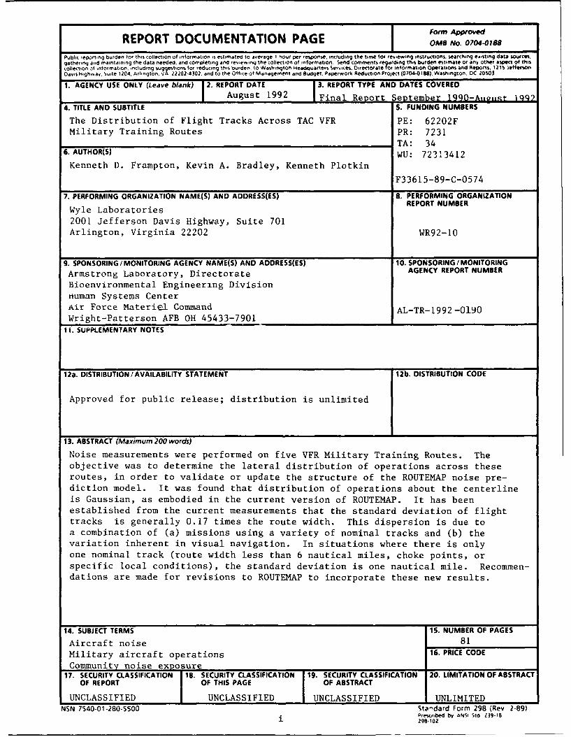
13. ABSTRACT (Maximum 200 words)
Noise measurements were performed on five VFR Military Training Routes. Theobjective was to determine the lateral distribution of operations across theseroutes, in order to validate or update the structure of the ROUTEMAP noise pre-diction model. It was found that distribution of operations about the centerlineis Gaussian, as embodied in the current version of ROUTEMAP. It has beenestablished from the current measurements that the standard deviation of flighttracks is generally 0.17 times the route width. This dispersion is due toa combination of (a) missions using a variety of nominal tracks and (b) thevariation inherent in visual navigation. In situations where there is onlyone nominal track (route width less than 6 nautical miles, choke points, orspecific local conditions), the standard deviation is one nautical mile. Recommen-dations are made for revisions to ROUTEMAP to incorporate these new results.
14. SUBJECT TERMS 15. NUMBER OF PAGES
Aircraft noise 81Military aircraft operations 16. PRICE CODE
Community noise exposure17. SECURITY CLASSIFICATION 18. SECURITY CLASSIFICATION 19. SECURITY CLASSIFICATION 20. LIMITATION OF ABSTRACT
OF REPORT OF THIS PAGE OF ABSTRACT
UNCLASSIFIED UNCLASSIFIED UNCLASSIFIED UNLIMITEDNSN 7540-01-280-5500 Standard Form 298 (Rev 2-89)
Prescribed by ANSI Std Z39-18298-102

THIS PAGE LE~T BLWN INTENTIatPALLY.
ii
TABLE OF CONTENTS
1.0 INTRODUCTION 1
2.0 TAC LOW-LEVEL TRAINING OPERATIONS.. ........ 4
2.1 Routes and Mission Profiles............ . 4
2.2 Operations and Scheduling............. 7
3.0 FIELD PROGRAM ................................ 10
3.1 Site Selection .............................. 10
3.1.1 VR-1220, Arizona ........................ 10
3.1.2 VR-223, Arizona . ........................ 12
3.1.3 VR-087, South Carolina ..................... 14
3.1.4 VR-088, South Carolina ..................... 14
3.1.5 VR-1074, North Carolina .................... 17
3.2 Instrumentation and Field Procedures ................. 17
3.2.1 Automatic Noise Monitors ................... 17
3.2.2 Field Service Procedures .................... 22
4.0 DATA ANALYSIS AND RESULTS ....................... 24
4.1 Data Analysis Procedures ........................ 24
4.2 Schedule Data and Measurement Correlation ............. 27
4.2.1 VR- 1220, Arizona ........................ 27
4.2.2 VR-223, Arizona ......................... 36
4.2.3 VR-087, South Carolina ..................... 37
4.2.4 VR-088. South Carolina ..................... 37
4.2.5 VR-1074, North Carolina .................... 38
4.3 MTR Measurement Results ....................... 38
4.3.1 VR-1220 Measurement Results ................. 43
4.3.2 VR-223 Measurement Results .................. 44
4.3.3 VR-087 Measurement Results .................. 49 D
4.3.4 VR-088 Measurement Results .................. 49 ----------
4.3.5 VR-1074 Measurement Results ................. 56
4.4 Noise Levels and ROUTEMAP Comparison . .............. 56ty Codes
hMvd: and Ioriii Dist S ,,
TABLE OF CONTENTS (Continued)
5.0 CONCLUSIONS ................................. 73
REFERENCES.................... R1
LIST OF FIGURESFig.XQo
1 Low-AltItude TAC Route: VR-223............. 5
2 Route Description of VR-223, From Reference 8.. ....... 6
3 VR-088 Mission Plan................ 8
4 VR-1220 Map . .................................. 11
5 VR-223 Map ................................... 13
6 VR-087 Map............................... .... 15
7 VR-088 Map ................................... 16
8 VR- 1074 Map . .................................. 18
9 Typical Monitor Installation .......................... 20
10 LD-700 and Battery Inside Environmental Case ................ 21
11 Excerpt From Typical Exceedance Report From VR-088 Site 17 25
12 Sound Level Distribution for a Two-Ship Formation ............. 26
13 VR-1220 Event Distribution . .......................... 39
14 VR-1220 Event Cumulative Probability Distribution ............. 40
15 VR- 1220 Total Events at Each Site ....................... 41
16 Distribution of Event Sound Levels, VR- 1220 ................. 42
17 VR-223 Event Distribution ........................... 45
18 VR-223 Event Cumulative Probability Distribution .............. 46
19 VR-223 Total Events at Each Site ........................ 47
20 Distribution of Event Sound Levels, VR-223 .................. 48
21 VR-087 Event Distribution ........................... 50
22 VR-087 Event Cumulative Probability Distribution .............. 51
iv

LIST OF FIGURES (Continued)Fig.
23 VR-087 Total Evc its at Each Site ........................ 52
24 Distribution of Event Sound Levels, VR-087 .................. 53
25 VR-088 Event Distribution ........................... 54
26 VR-088 Event Cumulative Probability Distribution .............. 55
27 VR-088 Total Events at Each Site ........................ 57
28 Distribution of Event Sound Levels. VR-088 .................. 58
29 VR- 1074 Event Distribution . .......................... 59
30 VR-1074 Event Cumulative Probability Distribution ............. 60
31 VR- 1074 Total Events at Each Site ....................... 61
32 Distribution of Event Sound Levels. VR- 1074 ................. 62
33 VR- 1220 Measured and Predicted Ld. ...................... 65
34 VR-223 Measured and Predicted Ld . ...................... 66
35 VR-087 Measured and Predicted Ldn . ...................... 67
36 VR-088 Measured and Predicted Ld . ...................... 68
37 VR- 1074 Measured and Predicted Ldn ...................... 69
LIST OF TABLESTableNo.
1 VR- 1220 Schedule 28
2 VR-223 Schedule . ................................ 30
3 VR-087 Schedule ................................. 31
4 VR-088 Schedule . ................................ 32
5 VR- 1074 Schedule ................................ 33
6 MTR Distribution Summary .......................... 70
v

THIS PAGE LEFT BLANK INTENTICtWILY.
vi

1.0 INTRODUCTION
Low-altitude, high-speed training operations are routinely conducted by all
Air Force flight operation commands. These operations are conducted on
specially designated Military Training Routes (MTRs).* Routes are continually
changed because of the need for variety, changing requirements of weapon
systems and tactics, and encroachment on existing routes. Environmental
assessments are required for new routes. A series of studies on MTR noisel-4 has
led to the ROUTEMAP model5 which is currently used for these assessments. 6
The main objective of this study was to further support the previous measurement
studies and to review (and modify, if necessary) the ROUTEMAP noise model-
ing program.5
Reference 1 contains an overview of MTR operations and identifies both
short- and long-term research which are needed in order to support environ-
mental assessments. Included in the short-term needs were measurements of
noise on two MTRs: one operated by SAC and one by TAC.** the two dominant
route users. SAC operates several dozen routes ranging in length up to 1,000 miles.
TAC operates several hundred routes with lengths typically between 100 and
300 miles. Recommendations were also made for psychoacoustic research needed
to understand the human effects of this type of noise environment, which is
sporadic in nature and different from the urban airport/highway environment
extensively studied for community response to noise.
Reference 2 contains the results of a measurement program on a SAC route.
SAC operations are conducted on Instrument Flight Rule (IFR) routes (denoted IR).
and involve point-to-point navigation using a variety of electronic aids. A key
finding of Reference 2 was that aircraft tend to be near the centerline of the route.
with deviation from the centerline being well described by a Gaussian distribution
with a standard deviation of 0.45 nautical mile.*** The noise levels of individual
MTR operations take place under waivers to FAR 91.117 (Aircraft Speed), which
normally limits speeds to 250 kt indicated airspeed below 10,000 feet MSL.
• * As of 1 July 92, SAC and TAC have been reorganized into Air Combat Command
(ACC).•* * Results of References 2 and 4 were presented in statute miles. This is incon-
sistent with the use of nautical miles for MTR descriptions and has proven tobe a significant inconvenience. In the current study, results are presented interms of nautical miles, and it is recommended that ROUTEMAP be modifiedto adopt this convention.
I
aircraft were found to be in good agreement with predictions from the Air Force's
NOISEFILE data base. Because of the limited variety of aircraft types involved
(almost all B-52 and B-I) and the centralized command and training structure of
SAC operations, it was concluded that these results can be generalized to all SAC
low-level routes. Reference 2 also contains anecdotal observations of residents'
reactions to low-level flight operations.
Reference 4 contains results from a similar measurement program per-
formed on two TAC routes. Most TAC operations are conducted under Visual
Flight Rules (VFR) on VFR routes (denoted VR). Many different mission types are
flown by TAC aircraft including ground attack, basic training, and others. There
were two important findings in Reference 4. First was that when a route section
had a single dominant track which the aircraft followed, the distribution of aircraft
was well defined by a Gaussian distribution of standard deviation 1. 1 nm.* Second,
if multiple tracks occurred within a route section, the distribution of aircraft was
well described by a Gaussian distribution with a standard deviation of about 2.2 nm.**
This report presents the results of similar measurements performed on five
additional TAC routes. The first two routes were located in Arizona and were
scheduled through Luke AFB. These routes were VR- 1220 and VR-223, and both
supported advanced student training operations. The third and fourth routes,
VR-087 and VR-088, were located in South Carolina. These routes supported air-
to-ground mission training for F- 16s out of Shaw AFB. The final route, VR- 1074,
was located in North Carolina. This route supported night-attack missions for
F- 15s from Seymour Johnson AFB.
Noise measurements were taken using from 16 to 30 automatic noise
monitors placed laterally across the route. Each time the noise level exceeded a
preset threshold, the monitors recorded the maximlm A-weighted sound level,
the time and duration of the event, and the sound exposure level. These data
were subsequently analyzed to determine the statistical distributions of maximum
sound levels (and hence aircraft tracks) relative to the route centerline.
* 1.25 statute miles.
* * 2.5 statute miles.
2
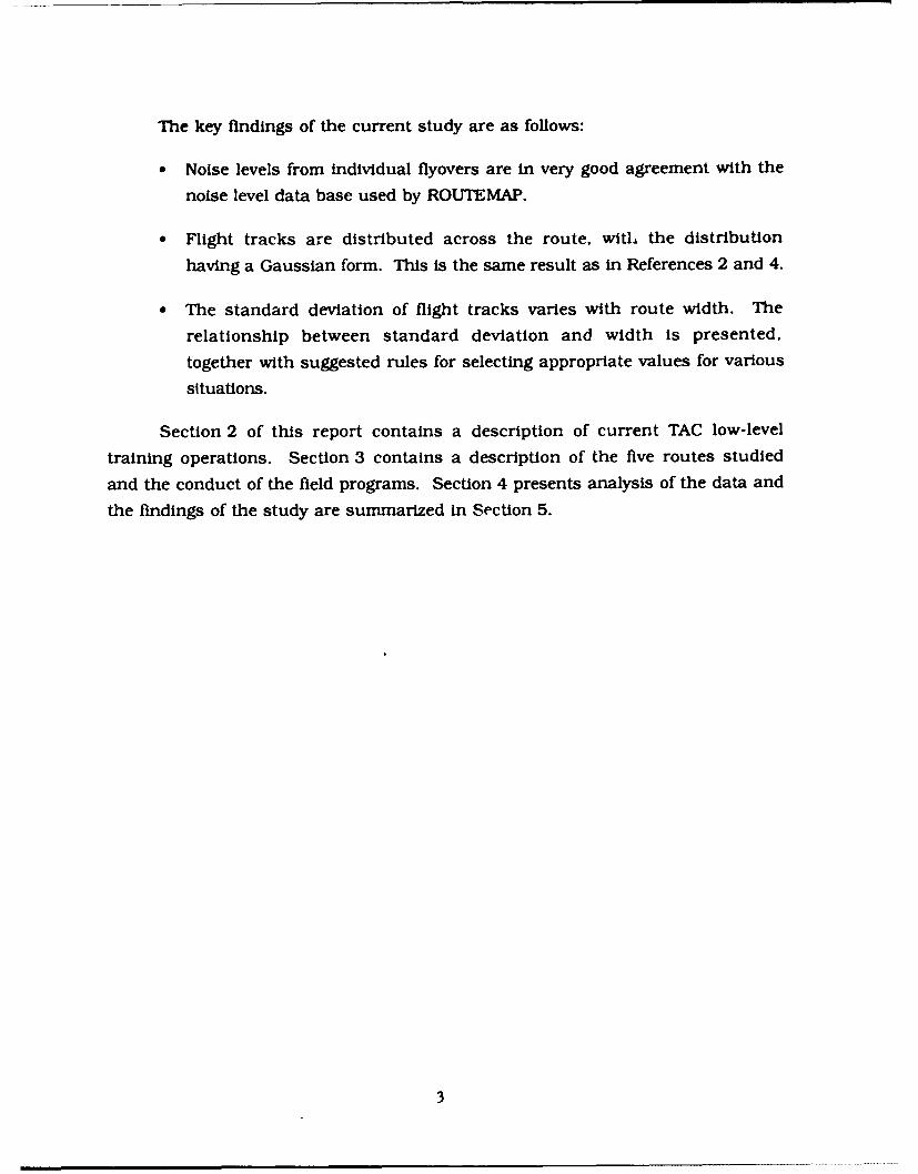
The key findings of the current study are as follows:
"* Noise levels from individual flyovers are in very good agreement with the
noise level data base used by ROUTEMAP.
"* Flight tracks are distributed across the route, with the distribution
having a Gaussian form. This is the same result as in References 2 and 4.
" The standard deviation of flight tracks varies with route width. The
relationship between standard deviation and width is presented,
together with suggested rules for selecting appropriate values for various
situations.
Section 2 of this report contains a description of current TAC low-level
training operations. Section 3 contains a description of the five routes studied
and the conduct of the field programs. Section 4 presents analysis of the data and
the findings of the study are summarized in Section 5.
3

2.0 TAC LOW-LEVEL TRAINING OPERATIONS
2.1 Routes and Mission Profiles
The Tactical Air Command conducts high-speed, low-level training
missions under visual flight rules. The objective of these missions (denoted air-to-
ground) is to practice low-level, point-to-point navigation. Current procedures
call for altitudes as low as 100 feet AGL and air speeds from 420 to 480 knots.
TAC aircraft involved include F-4s, F-15s, and F-16s. Navy, Marine, Air National
Guard, and Reserve units routinely fly similar missions on many of the same or
similar routes. The operations are qualitatively similar to SAC low-level missions
in that the aircraft are navigating to a destination, nominally following a series of
predetermined navigation points. There are inherent differences from SAC
operations due to the prevalence of visual flight rules for these routes: operations
tend to be during daylight hours, and navigation points are not crossed with the
same high degree of precision. Fighter aircraft also operate in multiple-ship
formations, which can be over a mile wide. Most flights have two or four aircraft.
A typical two-ship formation is line abreast, where the aircraft are even with each
other and laterally separated by 6,000 to 8,000 feet. An alternative is for the
second aircraft to fly in trail, 10,000 to 15,000 feet behind the leader. On occa-
sion, two aircraft will fly in a close echelon, separated by a few hundred feet, but
this is relatively uncommon. Four aircraft fly in box formation, consisting of two
lines abreast with the second line following the first by 10,000 to 15,000 feet.
The second line is usually offset about half the line width. Wide formations tend
to change structure, then reform as they negotiate turns, mountain passes,
ridges, etc.
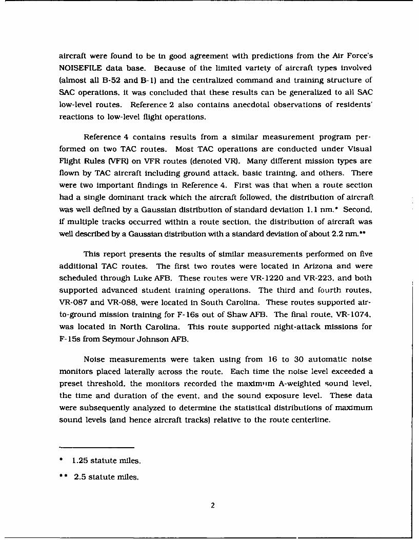
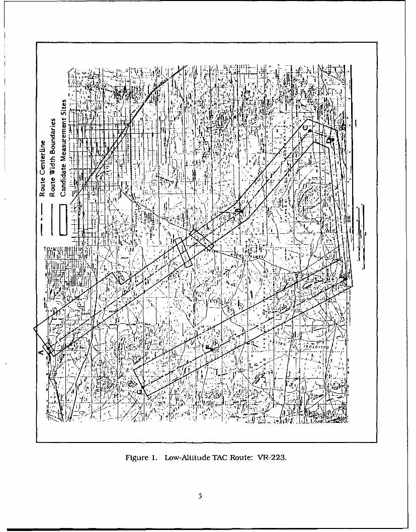
Figure I shows a typical TAC route, VR-223 in southern Arizona. Shown are
the centerline and edge boundaries. Also shown are candidate measurement sites
which had been considered for measurements on this route. 7 Official route
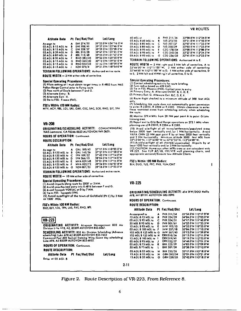
descriptions are published in the AP/ 1B booklet. 8 Figure 2 is the published
description of VR-223 taken from Reference 8. The approach to primary entry
point A is specified as 6,000 feet MSL (about 4,500 feet AGL), with the remainder
clear for 500 feet AGL. Minimum published altitudes are based on obstacle
clearance, and on many routes are 100 feet AGL or surface. Higher limits imposed
by the command supersede these. While the route may be entered or exited at a
number of points, it is typical to use the primary entry and exit. The route width
4
I Jlý ~
T -I I
fV,,4)f _ _L --
.. I iI/ . 4.
Figure~~~~~ 1 o litd A oueV 2
4v5
VR ROUTES
Altitude Data Pt Fac/Rad/t0lst Lat/Long 60 MSI. ot A PHX 211/36 33*00.0'N 11I 2*24.0'W05 AOL 860 MSL to 8 TUS 2)2/55 32*21.O'N I11 *51.0'W
As asgn to A ENi 2.74/50 39-22,0'N 1246 IO'W 05AGL 8 80 MSE to C TIJS 257/37 32*07.0'N I11l'33.0O'W02 AG08 15 AGE to IS ENI 308/41 39*37f'N 123*46.0'W 05 AGL 880MSL to D IUS 250/39 32'02.5N I I1'35.0'W02 AGL 8 15 AGL to C ENI 328!37 3939,0'N 123*28.0'W 05 AGL 8 90 MSL to E CZG 178/54 32*00.0'N I 12*08.0'W02 AGE B30AGL to 0 RBL 210/28 39*47.0'N 122*41.0'W 05 AGI 8 90 MSL to F CZG 210/36 32*27.0'N I I2'24.5'W30 AGE 8 80MSL to E ROIL 112/48 39'35.014 l21 27.0'W 05 AGL 89OmSt to G CZG 236/35 32'41.0'N 112*33.0'W02 AGL 8130 AGL to F RNO 282/45 39*54 O'N 20*30.0OW02 AGL B 15 AGLE to RN0 345/40 40*120ON 119*37.0'W TERRAIN FOLLOWING OPERATIONS: Authorized A to E.02 AGL 8 15 AGL to H RNO 054/33 39542.314 11 t859.0'W ROUTE WIDTH - 2 NM irght and 5 NM left of cienterlins. A to02 AGLS 9 5 AOL to I HZN 073/4 39*31.0'N I 18*54.0-W 32*44'OO"N 1 12'11'00W; 2 NM either aide of centerlineiTERRAIN FOLLOWING OPERATIONS: Authorized entire route. 32*" 04400N 112*1 I'00'W toOD; I NM either side of centerline, D
ROUT WIDH -2 NMeiter sde o ceteflne.to E; 2 NM left and 4 NM rig~it of centerline, E toOG.
Special Operating Procedures: Special Operating Procedures:(1) ilos eitig atI mst btan tagettims i R-403 romNAS IfI Contact scheduling activity for route briefing.(I) ilos eitig a I ustobtin argt tmesin -483 fom AS 21 Turn radius based on 420 KIAS.
Fallon Range Control prior to flying route. (3) Tie in FSS: Phroenix IPHXI. Contact prior to entry.(2) Pass north of Doyle between F and G. (4) Primary Entry: A. Alternate ENTRY: 8, C, 0, E.(3) Alternate Entry: B. (.5) Primary Exit: G. Alternate Exit: BC, 0, E. F.(4) Alternate Exit: H.(5) Tei S:Fen(FT.(6) Route flight checked to a minimum altitude of 500 feet AOL
Tie-n FS: resn (FT).only.FSS' Witin 10 NMRadis:(7) Scheduling this route does not automatically grant permissionFSS' Witin 00 N Radus:to enter R-2301E, R-2304 or R-2305. Obtain clearance to enter
MYV, ACV, R8L, LOL, UIKI, OAK, CEC, SAC, SCK, RNO, Sly, TPH these 'eitricted areas from scheduling activity when schedulingthe route.
(8) Monitor 379.4 MHz from 20 NM post point A to point G-Latntraining area.19) Report exit to Gila Bend Range operations on 272.1 MHz when
VR-208 planning use of R.2301E, R-2304 or R-2305.
ORIGINATINGISCHEDULING ACTIVITY: COMLATWINGPAC (10) Avoid o~erfiight of all to.mns/xettlements/populated areasNAS Lemtoore. CA 93246-0022 AUTOVON 949-3631. below 3000 feet vertically and /or 1 NM horizontally. Avoid
VAYA CHIN 23 NM past point E by at least 3000 feet verticallyHOURS OF OPERATION: Continuous, and 2 NM horizontally. Minimum altitude 5000 feet MSL from
ROUTE DESCRIPTION: 32*13'00'N. I12*1600"W to 32'27'00"N, 1 12*24'00"W.(I1I) Avoid overflight of all charted/ uncontrolled Airports by at
Altitude Data Pt Fac/Rad/Dist Lat/Long least 1500 feet vertically and/or 3 NM horizontally.
As asgn to A CAL 180/45 37-17.0'N 118-03.0:W 112) CAUTION: Numerous other MTRs Cross or ore coincident with02AGL 8 130 MS1 to 8 OAL 142/36 37*27.0'N 117*30.0 W VR-223.I See FLIP AP/IB, IFR/VFR wail planning charts, and02 AOL 8 130 MSL to C IPH 189/22 37-42.0'N 117-14.0-W appropriate sectional/ Enroute Low Altitude Charts.
02 AOL B 130 MSL to D IPH 266/t10 38*04.0'N 117*14.0'W02 AOL 8 100 MSIL to E MVA 039/48 39*01 -ON I11711 I .W FSS's Within 100 NM Radius:02 AGL 8 120 MSIL to F MVA 022/72 39-24.0'N 116*57.0'W 8tH, DUO, TUS, PRC, PHX. YUM.ONT02 AGE 8 120 MSL to G HZN 087/53 39'18.0'N 1 17-53.0'W
TERRAIN FOLLOWING OPERATIONS: Authorized entire route.
ROUTE WIDTH - 10 NM either side of centerline.
Special Operating Procedures:(1) Avoid airports along route by 2000' or 3 NM. VR-225(2) Avcid unauthorized entry into R-4816 between F and G.(3) Avoid Tonopah VORTAC ot D by 7 NM.(4) Tie-in FSS: Tonopahs (TPHI. ORIGINATING/SCHEDULING ACTIVITY: 474 TFW/DOO Nelis(5) Avoid overflight of the town of Goldfield (Pt C) by 3 NM AF8, NV 89191 AUTO VON 682.2090.or 1500' AGL. HOURS OF OPERATION: Continuous.
FSS's Within 100 NM Radius: ROUTE DESCRIPTION:EKo, ELY, LOL, IPH, LAS, FAT, RNO, BFIL Altitude Data Pit Fac/Rad/DIst Lat/ Lang
As asstqned to A PHX 311/34 33*54.0'N 112*17.O'W
1 5 AOL 8 75 MSL to 8 PHX 334/39 34*04.O'N Ii2*03.0'W0523O AOL 8 95 MSL to C PHX 354/51 34x17.O.N 111*45.0'W55MSL S 95 MSL to D PHXO001/61 34*25.0'N I1II133.5'W
ORIGINATING ACTIVITY: Airspace Management 832 Air 15 AGL 8 95 MSL to E INW 193/13 34'52.0'N I I 055.0'WDivislon L"Ire AF8, AZ, 85309 AUTOVON 853-6067. 105AGL 8105 MSL to F INW 257/I8 35*04.0'N I11x10,0'W
SCHEDULING ACTIVITY: 832 Air Division Scheduling (Advance 105 MSL B 125 MSL to G INW 267/43 35*12.0'N I1II139.O'Wscheduling) Luke AFS AZ 85309 AUTOVON 853.7653 105 MSL 8 125 MSL to H DRKOIO/36 35*1 5.0'N 112'1 1.0'WCommand Post 405 Tactical Training Wing (Some day scheduling) 15 AOL B 105 MSL to I DRK319/41 35*19.0'N 11 2*52.0'WLuke AFB, AZ 85309 AUTOVON 853.6022. 05 AOL 8 95 MSIL to J DRK252/27 34*40.(YN I13*01.0'W
HOURS OF OPERATION: Continuous. 05 AOL 8 75 MSL to K BXK 322/39 34*03.0'N I 13*09.0'W55 MSL 8 75 MSIL to L BXK 307/30 33*50.5'N 113*12.0'W
ROUE DSCRPTIN:05 AOL 8 55 MSL to M BXK 233/26 33'17.0'N 1 13*18.0'WAltitude Data Pit Fac/Rad/Dist Lat/ Long 15 AGE 8 55 MSL to N GBN 262/34 33*0l.0'N 113*21.0'W
Enera 0 OL815 AOL 8 35 MSL to 0 GBN 230/35 32*42.0'N 1 13*18.0'W
2-11
Figure 2. Route Description of VR-223, From Reference 8.
6

varies, based on clearance of known obstacles and avoidance of noise-sensitive
areas such as population centers and recreational areas. Typical widths rangefrom 4 to 20 nautical miles; segment D-E of VR-223 is 2 miles wide. There is no
formal lateral constraint except to remain within the route boundaries. At the
speeds involved and with visual navigation, events happen very quickly as the pilot
watches for landmarks several miles ahead, so that the tendency is to remainwithin the center part of the corridor.
Prior to a mission a tentative flight plan is prepared by each pilot. Thisplan is sketched on a map containing the route outlines along with notes on
headings, obstacles, and areas to avoid. Figure 3 shows one such mission plan for
VR-087 in South Carolina. A path is drawn between navigation points within the
boundaries of the MTR These navigation points appear as circles in Figure 3 and
usually correspond to prominent landmarks. In addition, the mission plan hasone navigation point labeled with a square followed by a point labeled with a
triangle. The square navigation point denotes a check point which orients themission towards the simulated target labeled with the triangle.
Not every mission uses a unique flight plan; this depends on particulargoals. For example, in student pilot training, emphasis is on aircraft handling. In
that case, only the instructor pilot leading the flight will have a mission plan, and
that will be a standard chart used repeatedly for that route.
2.2 Operations and Scheduling
The busiest TAC routes are scheduled for 2,000 to 3,000 sorties per year.Based on 200 flying days per year, there will be an average of 10 to 15 sorties(grouped in three to five missions) per day on these busy routes. Minimumheadway between flights is 5 minutes, although the average time between flights is
much greater. The rate of flights is comparable to that on SAC routes (average offive flights per day on the busiest routes2), and is comparably sporadic. Each flight
is essentially an isolated event, so that there is no reason to expect missionprofiles on busy routes to differ from those on lightly used ones. As was done for
the previous route measurements, 2.4 the TAC routes selected for this study were
busy ones for which relatively large amounts of data could be collected in a
reasonable time.
7
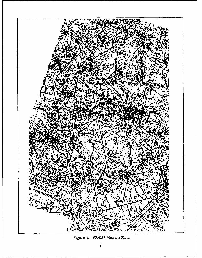
Figure 3. VR-088 Mission Plan.

Scheduled activity for TAC routes is decentralized, with responsibility
handled by the primary route user. Route descriptions in the AP/lB booklet8
identify the scheduling activity plus appropriate military or civil air traffic control.
The purpose of scheduling is to avoid conflicts between users, without uni'eason-
ably restricting the flexibility and initiative implicit to tactical air operations. A
secondary use of schedule information is that these data can be analyzed to assess
the utilization of various routes, and thereby aid in airspace planning. This form of
schedule data is of interest in the current project, but it must be kept in mind
that available data are not collected for that purpose.
Scheduling is performed with various degrees of advance and short-termplanning. Reservation of specific time slots for particular missions generally takes
place the evening before or the morning of a mission. However, same-day
scheduling can occur up to aircraft launch time. At some bases, where local
weather changes rapidly, pilots may only schedule that they are doing a low-level
mission, and select the route based on conditions after launch. Actual route entry
times are usually within 15 minutes of scheduled times. Aircraft can also fly many
routes without advance schedule by obtaining clearance from the appropriate air
traffic control center. The schedule log will not reflect this unscheduled activity,nor will it account for mission cancellations. There are also occasional incidents
of aircraft flying routes without schedule or clearance. Usually, these are aircraft
at slower speeds (below 250 kts) under visual conditions, whose operations fall
within FAR 91.117 (Aircraft Speed), and therefore do not need to schedule special
use airspace.
Schedule data used in this study represents the records kept by the routeoperators. Data were collected after each flying day. They are therefore expected
to include all scheduled missions which flew, and also include missions which
were scheduled but cancelled.
9
3.0 FIELD PROGRAM
3.1 Site Selection
Measurement sites were selected on five MTRs based on the following
criteria:
1. Two routes in a western desert area, and three in an eastern forested
area. Differences in aircraft and/or operations were also desirable.
2. Areas of relatively flat terrain, to measure activity where altitudes would
be lowest and with minimal site-specific constraints.
3. Existence of a reasonably accessible road crossing the route, suitable fordeploying noise monitors.
4. High level of flight activity.
Sites meeting these criteria were found along VR-1220 and VR-223 in Arizona,
VR-087 and VR-088 in South Carolina, and VR- 1074 in North Carolina. Each of
these routes is described in detail in the following sections.
3.1.1 VR-1220. Arizona
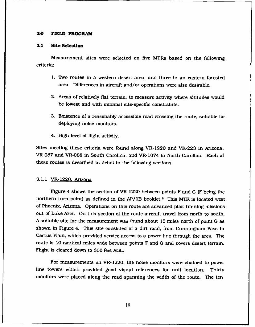
Figure 4 shows the section of VR- 1220 between points F and G (F being the
northern turn point) as defined in the AP/ IB booklet. 8 This MTR is located west
of Phoenix, Arizona. Operations on this route are advanced pilot training missions
out of Luke AFB. On this section of the route aircraft travel from north to south.A suitable site for the measurement was f-)und about 15 miles north of point G as
shown in Figure 4. This site consisted of a dirt road, from Cunningham Pass to
Cactus Plain, which provided service access to a power line through the area. Theroute is 10 nautical miles wide between points F and G and covers desert terrain.
Flight is cleared down to 300 feet AGL.
For measurements on VR- 1220, the noise monitors were chained to power
line towers which provided good visual references for unit location. Thirtymonitors were placed along the road spanning the width of the route. The ten
10
12A
PRES470T
tXý. CAlt;`ý P. ./ý- . ' -A - . . .
7.
e
WWI 42
v
G LA D-6 E- N
NG 00
Y245
24 73 - 35 f 22.9
lodr
00L thn
ent OAS
m
vi 14
so
Figure 4. VR- 1220 Map.
monitors which straddled the route centerline were separated by a one-quarter-mile interval. This interval progressively increased to a maximum of one milebetween the last three monitors at either edge of the route. This intervalarrangement maximized the density of monitors near the route centerline wheremost of the air traffic was expected.
As can be seen in Figure 4. there are several other MTRs which overlapparts of the measurement array. These include VR-245, VR-283, VR-1267,VR-1268, IR-214, and IR-272. The air traffic along these routes could have beenrecorded by the noise monitors. Schedule data for VR-245 was available whichallowed missions on this route to be removed from the data. The other routeswere identified as being lightly used.
Arrangements were made with the 832nd Air Division to obtain scheduleinformation for the measurement period of 3 March 1991 to 31 March 1991 forVR-1220 and VR-245.
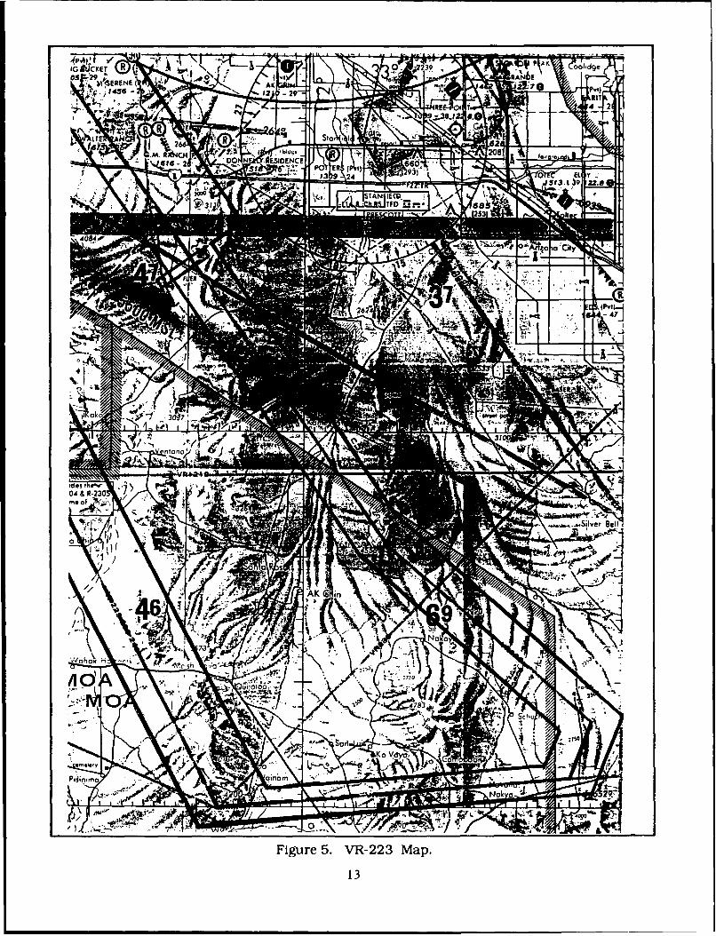
3.1.2 VR-223. Arizona
Figure 5 shows most of VR-223, which is located south of Phoenix, Arizona.Operations on this route are advanced pilot training missions out of Luke AFB. Themeasurement site selected for this route was located between points A and B ofthe route8 as shown in Figure 5. Air traffic travels in a clockwise direction aroundthe MTR. From point A to a point along the route near the measurement site theroute is 7 nautical miles wide: 2 nautical miles left and 5 nautical miles right of thecenterline. After this point the route boundaries are 2 nautical miles either sideof the centerline. Flight is cleared down to 500 feet AGL between points A and B.The terrain below this section of the route was desert.
The measurement site, indicated in Figure 5, was along a dirt road throughthe Vekol Ranch. This is at the point where the route narrows from 7 to 4 nauti-cal miles. The Tabletop Mountains obstruct the eastern quarter of the route, sothis location is a choke point with an effective width of about 3 nautical miles.Sixteen monitors were deployed across this portion of the route, at 0.25 statutemile intervals, from 0.5 mile west of the western boundary to 1.5 miles east of theroute centerline.
12
4P`I`1UcXETV' R P AKIG,1 ge
, fV,-29 0\ E% EREýSERE 70
12 1-29-- J. ?e RIT
CVR 2
E
LT A2"
-Do N RESIDENCE 20
, V
J 313 L ýq .8
S IUD..=TF 68i
1253
y
R
cP_El
4
Wr
I OW -7 30377
Mon
& Olt 't
---- Silver Belli
r
,7
K in
7,3
A _nj0 k
M
Alý'h
Sari
KoV
PI'vnimo 3mom
Nok 2
Lo, JIM6 ý 7-wi, i --ýýIýFigure 5. VR-223 Map.
13

Arrangements were made with the 832nd Air Division to obtain scheduleinformation for this route. No other MTRs were in the vicinity of the measure-ment array.
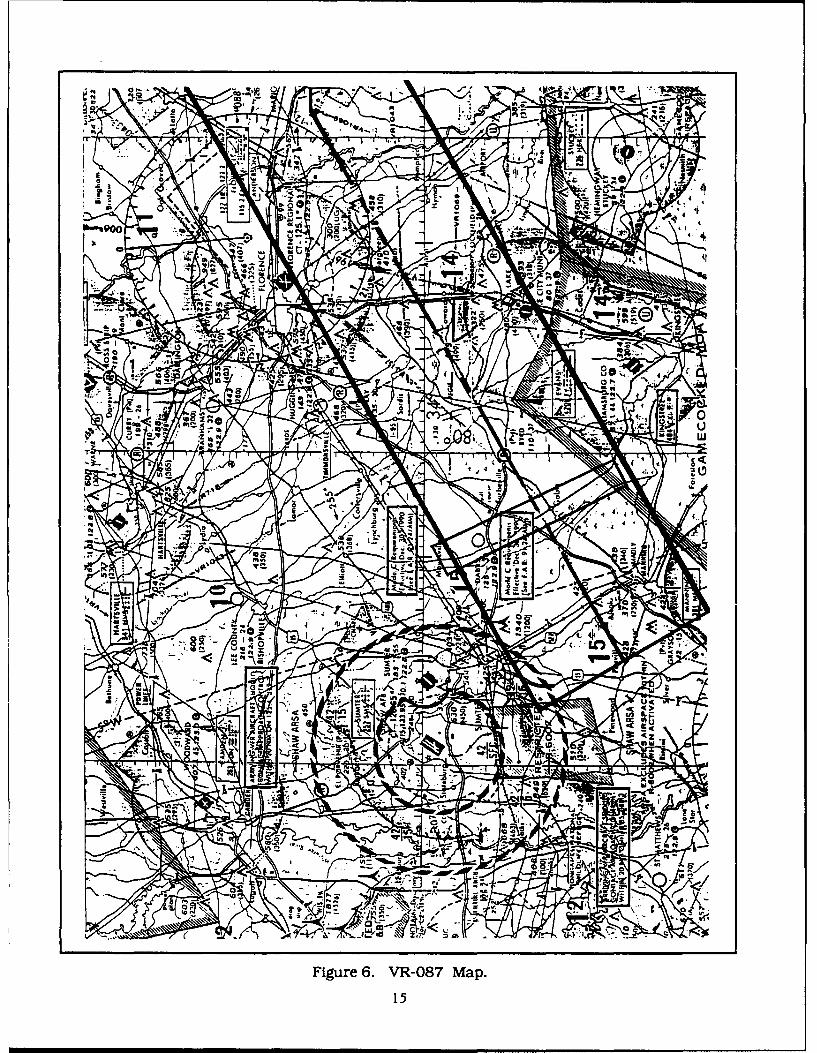
3.1.3 VR-087. South Carolina
This route is located east of Sumter, South Carolina. Operations along thisroute consisted of ground attack readiness training by F-16s stationed at
Shaw AFB. Figure 6 shows the leg of VR-87 between points E and F whereoperations travel west. This segment of the route is 16 nautical miles wide andflight is cleared down to 100 feet AGL. A suitable measurement site was locatedalong a rural highway as depicted in Figure 6. The terrain under this leg of theroute is rural forests and agricultural fields.
The measurement array was located along SC Route 527. Twenty-eightmonitors were placed about 0.7 mile apart along the side of the road and werechained to telephone poles. This arrangement spanned the entire route, althoughthe wide spacing did reduce the resolution of the noise measurements.
Arrangements were made with the 363rd Fighter Wing at Shaw AFB toobtain schedule information for the route.
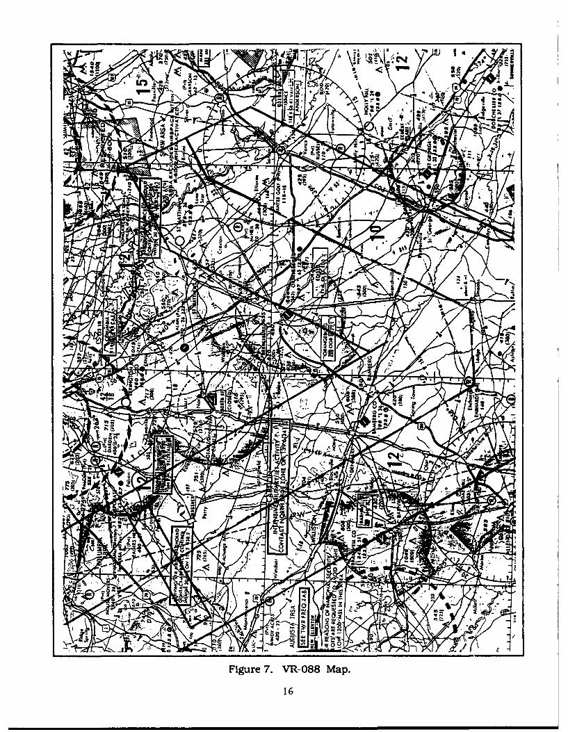
3.1.4 VR-088. South Carolina
Operations along this route consisted mainly of ground attack readinesstraining by F- 16s stationed at Shaw AFB. Figure 7 shows part of VR-88 betweenpoints C and G where operations travel southeast. The measurement site selected,as shown in Figure 7, was located Just east of Aiken, South Carolina. The route
along this leg is 20 nautical miles wide. Flight is cleared down to 300 feet AGL.The terrain under this leg is mostly rural forests and agricultural fields.
The measurement array was located along several rural roads, stretchingfrom 8 miles east of Aiken, SC, through the town of New Holland, SC (under theroute centerline), to the town of Fairview Crossroads, SC. Twenty-seven monitorswere distributed across this route. The monitors within 3 miles of the routecenterline were spaced 0.5 mile apart. Monitors beyond this range were spaced
14
I-L's
crJ
sour E.V -87Mp
15X
C%4
ZN
my
W-Z 0LLK
A
iz
-Pe
so
Nl-
ýr3
17
ivy
Z_-N0 j5
09 In
0In w-
o
Figure 7. VR-088 Map.
16
about 0.6 mile. This spread left about 2.5 miles at either edge of the route without
monitor coverage, but heavy use was not expected at the edges.
Arrangements were made with the 363rd Fighter Wing at Shaw AFB to
obtain schedule information for the route.
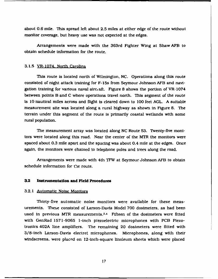
3.1.5 VR-1074. North Carolina
This route is located north of Wilmington, NC. Operations along this route
consisted of night attack training for F- 15s from Seymour Johnson AFB and navi-gation training for various naval airc, aft. Figure 8 shows the portion of VR-1074between points B and C where operations travel north. This segment of the routeis 10 nautical miles across and flight is cleared down to 100 feet AGL. A suitablemeasurement site was located along a rural highway as shown in Figure 8. The
terrain under this segment of the route is primarily coastal wetlands with somerural population.
The measurement array was located along NC Route 53. Twenty-five moni-
tors were located along this road. Near the center of the MTR the monitors werespaced about 0.3 mile apart and the spacing was about 0.4 mile at the edges. Onceagain, the monitors were chained to telephone poles and trees along the road.
Arrangements were made with 4th TFW at Seymour Johnson AFB to obtain
schedule information for the route.
3.2 Instrumentation and Field Procedures
3.2.1 Automatic Noise Monitors
Thirty-five automatic noise monitors were available for these meas-
urements. These consisted of Larson-Davis Model 700 dosimeters. as had been
used in previous MTR measurements. 2.4 Fifteen of the dosimeters were fittedwith GenRad 1571-9065 1-inch piezoelectric microphones with PCB Piezo-
tronics 402A line amplifiers. The remaining 20 dosimeters were fitted with
3/8-inch Larson-Davis electret microphones. Microphones, along with theirwindscreens, were placed on 12-inch-square linoleum sheets which were placed
17

ON 'Co•3 ,e7 1 -r3R
128 A" (43A0551 ELLA
w 3! -ý !ý . D ., v/
Manla 117, CZI I hit
1 1 .5 o
S. .• r.1- 170o,-
Fiur an V3- 1074Ma)
MCSIEWRV

on the ground. Each LD-700, together with a battery, was placed in an environ-mentally sealed container. Figure 9 shows a typical monitor site installation.Figure 10 shows the LD-700 and its battery inside the container. Field calibrationof the monitors was accomplished using a B&K Type 4230 calibrator.
The LD-700 is a microprocessor-based digital integrating sound levelmeter. It can be programmed to record interval, exceedance, and history data.Interval data consists of Leq and percentile exceedance levels. Exceedance dataconsists of records of levels that exceed a preset threshold. History data consistsof time histories of noise. The unit can be programmed to record A- orC-weighted levels, slow or fast detector response, and to integrate with 3. 4. or5 dB/doubling of time tradeoffs, corresponding to Leq, DoD noise dose, and OSHAnoise dose. The primary information collected for this project was the exceed-ance data. The threshold was generally set to 65 dB. It was set higher at siteswith significant extraneous noise, so as to avoid recording excessive spurious data.The highest threshold used was 70 dB.
The LD-700s have a bidirectional computer interface. This port can beused to program the unit Wnd to read data from It. A Toshiba T1200XE laptopcomputer was used for this purpose. The T1200XE is 80286 based, batterypowered, has a 3.5-inch floppy disk drive, and operates under the MS-DOSoperating system. Software developed for previous MTR measurements 4 was usedto initialize and program the LD-700s, and to read data and store them forsubsequent analysis. The initialization routine included setting the LD-700'sinternal clock, so that all monitors were time synchronized.
A maximum of 30 monitors was installed on a given MTR The remainingfive monitors were used as spares when installed units failed. The monitors wereplaced along rural roads and chained to convenient anchors for security (powerline towers, telephone poles, or trees).
The monitors were placed at optimum intervals across the MTRs such thatas many as possible would record an overflight. Therefore, if a particular monitorwas not operating when an overflight occurred, several other monitors wouldcapture the event. This aided in the identification of overflights from the monitordata. Other considerations in the monitor separation intervals were the width ofthe route to be covered and the availability of convenient anchor sites.
19
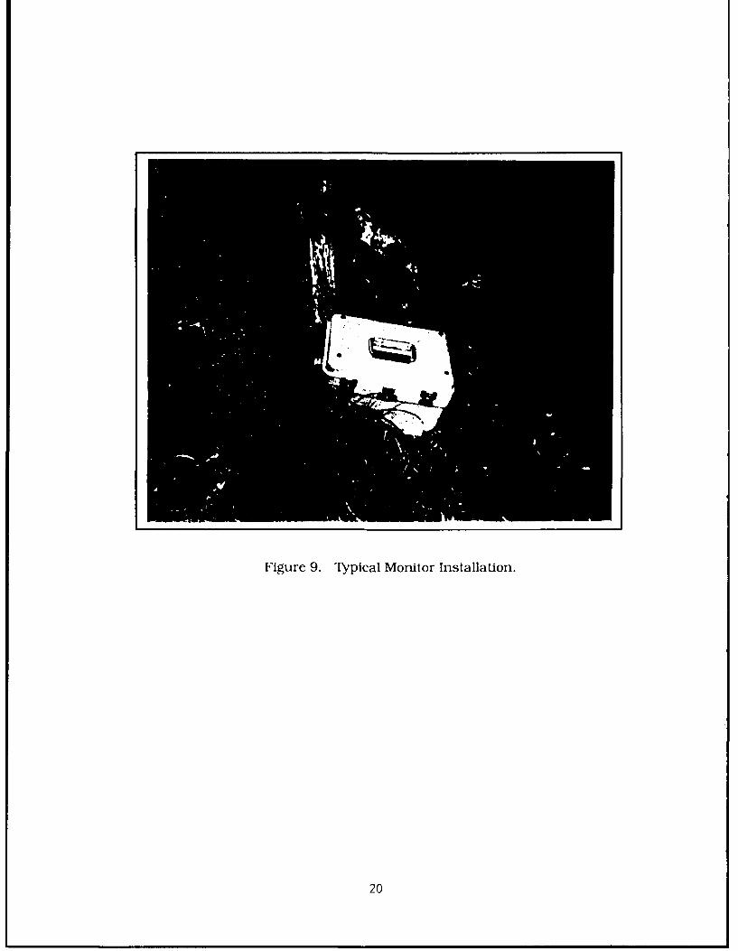
Figure 9. Typical Monitor Installation.
20
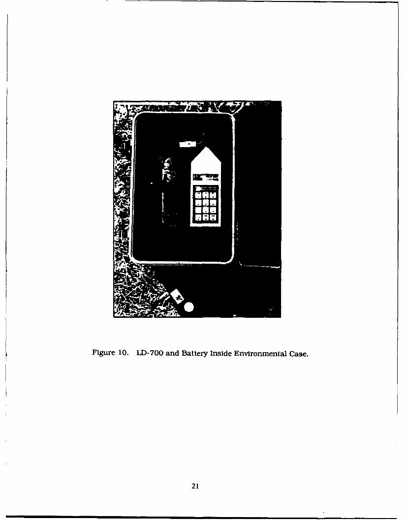
Figure 10. LD-700 and Battery Inside Environmental Case.
21
3.2.2 Field Service Procedures
Following initial installation, the monitors were checked once per day. A
check-up visit would proceed as follows:
1. The unit was approached and a visual inspection made of the site. The
time of day was noted on the daily log.
2. The environmental case was opened. The basic operation of the unit
was checked by observing the unit response to noise events.
3. The memory status of the unit was checked and noted in the daily log.
If a substantial amount of the memory was full. the download/reset
procedure was performed. If only a small portion of the memory was
occupied with data, the site visit was continued with step 7. below.
4. Monitors with a substantially full memory were stopped at this point.
The calibrator was placed on the microphone and the unit restarted.
This ensured that the last exceedance in the memory was the calibration
signal. The measured calibration level was noted in the daily log and the
unit turned off.
5. The unit was removed from the environmental case and interfaced with
the laptop computer. All exceedance histories were downloaded from
the unit and the operation parameters (including the internal clock)
were reset.
6. The unit was then returned to its environmental case and the calibration
signal was again recorded. This ensured that the first exceedance
record was the calibration tone. If necessary at this point, the unit cali-
bration was adjusted. The unit was restarted and the time was recorded
in the daily log.
7. Battery voltages were checked and recorded in the daily log. If
necessary, the battery was replaced with a fresh one. Also, any faulty
components were replaced or repaired.
8. Finally, the environmental case was closed and locked.
22
Depending on the noise environment in which a monitor was located, data
were download, :t most every day and at least every third day. Occasionally the
memory in a unit would be full due to a lost windscreen, livestock or rodent
interference, or other unpredictable events. In this case, the unit would be
inoperable until the next site visit.
If a particular unit was discovered to be dysfunctional, the unit was pulled
from the field and replaced with a spare. The rechargeable batteries usually
lasted 7 to 10 days before replacement was necessary.
23
4.0 DATA ANALYSIS AND RESULTS
4.1 Data Analysis Procedures
Following completion of the field programs, data from the monitors werecollated and correlated with the route schedule and field log. This informationwas compiled into an inventory of events from which statistical and other con-clusions could be drawn. Reduction of the data consisted of the following steps:
1. A composite list of scheduled and observed flights was compiled.
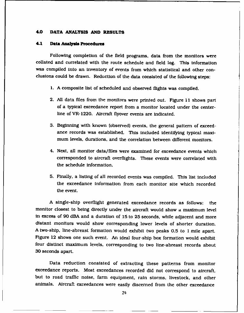
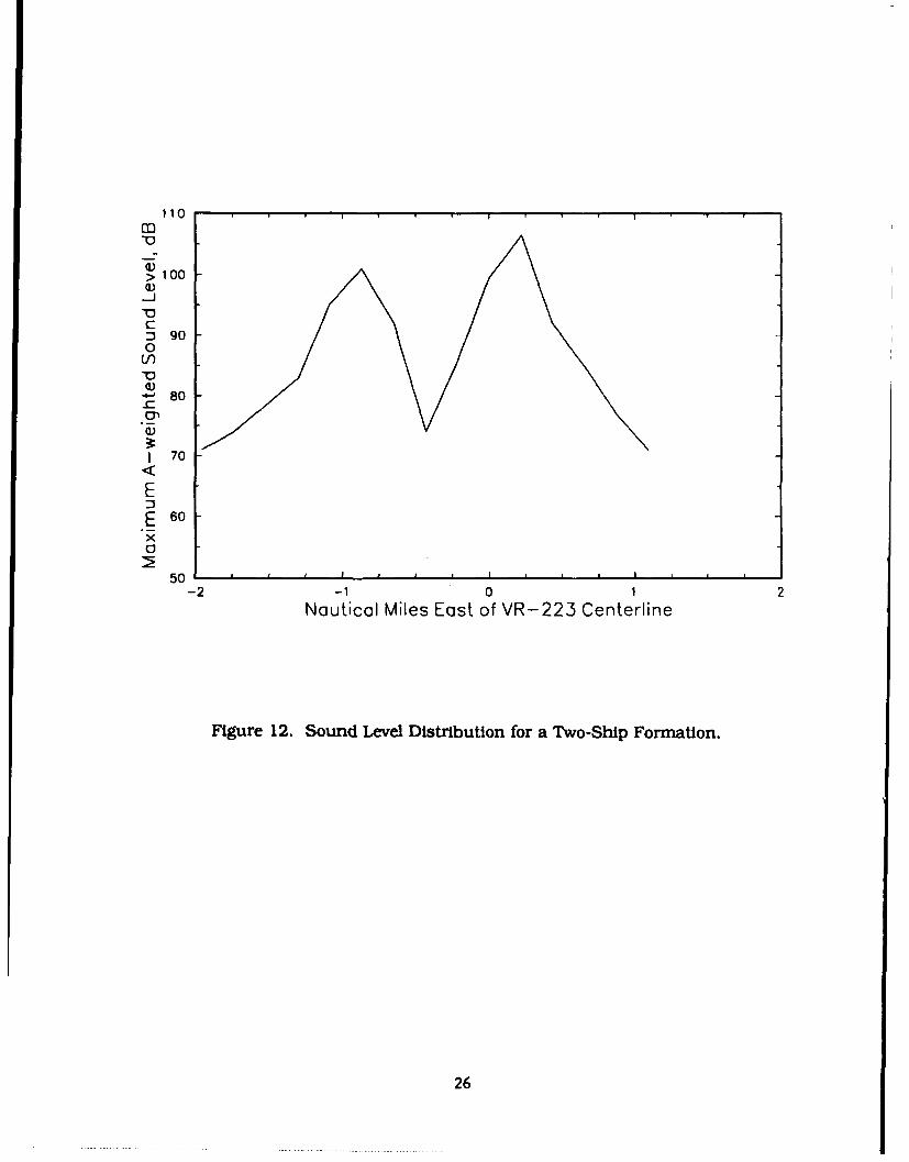
2. All data files from the monitors were printed out. Figure 11 shows part
of a typical exceedance report from a monitor located under the center-
line of VR- 1220. Aircraft flyover events are indicated.
3. Beginning with known (observed) events, the general pattern of exceed-
ance records was established. This included Identifying typical maxi-mum levels, durations, and the correlation between different monitors.
4. Next. all monitor data/files were examined for exceedance events whichcorresponded to aircraft overflights. These events were correlated with
the schedule information.
5. Finally, a listing of all recorded events was compiled. This list included
the exceedance information from each monitor site which recorded
the event.
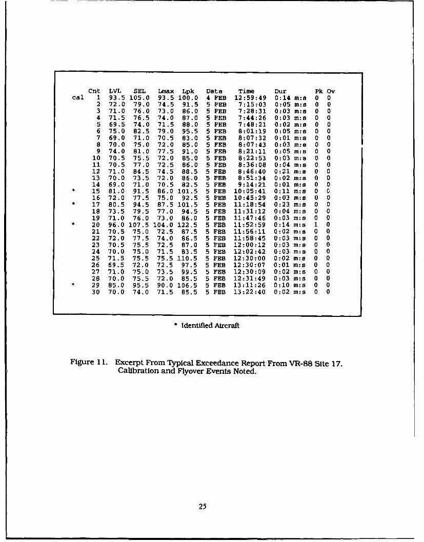
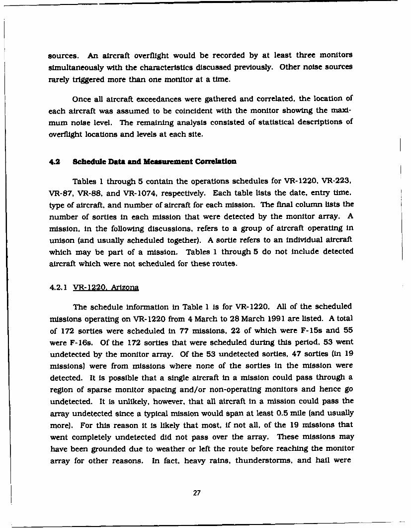
A single-ship overflight generated exceedance records as follows: themonitor closest to being directly under the aircraft would show a maximum level
in excess of 90 dBA and a duration of 15 to 25 seconds, while adjacent and moredistant monitors would show corresponding lower levels of shorter duration.A two-ship, line-abreast formation would exhibit two peaks 0.5 to I mile apart.Figure 12 shows one such event. An ideal four-ship box formation would exhibit
four distinct maximum levels, corresponding to two line-abreast records about
30 seconds apart.
Data reduction consisted of extracting these patterns from monitorexceedance reports. Most exceedances recorded did not correspond to aircraft,
but to road traffic noise, farm equipment, rain storms, livestock, and other
animals. Aircraft exceedances were easily discerned from the other exceedance
24
Cnt LVL SEL Lmax Lpk Date Time Dur Pk Ovcal 1 93.5 105.0 93.5 100.0 4 FEB 12:59:49 0:14 m:s 0 0
2 72.0 79.0 74.5 91.5 5 FEB 7:15:03 0:05 m:s 0 03 71.0 76.0 73.0 86.0 5 FEB 7:28:31 0:03 m:s 0 04 71.5 76.5 74.0 87.0 5 FEB 7:44:26 0:03 m:s 0 05 69.5 74.0 71.5 88.0 5 FEB 7:48:21 0:02 m:s 0 06 75.0 82.5 79.0 95.5 5 FEB 8:01:19 0:05 m:s 0 07 69.0 71.0 70.5 83.0 5 FEB 8:07:32 0:01 m:s 0 08 70.0 75.0 72.0 85.0 5 FEB 8:07:43 0:03 m:s 0 09 74.0 81.0 77.5 91.0 5 FEB 8:21:11 0:05 m:s 0 0
10 70.5 75.5 72.0 85.0 5 FEB 8:22:53 0:03 m:s 0 011 70.5 77.0 72.5 86.0 5 FEB 8:36:08 0:04 m:s 0 012 71.0 84.5 74.5 88.5 5 FEB 8:46:40 0:21 m:s 0 013 70.0 73.5 72.0 86.0 5 FEB 8:51:34 0:02 m:s 0 014 69.0 71.0 70.5 82.5 5 FEB 9:14:21 0:01 m:s 0 0
* 15 81.0 91.5 86.0 101.5 5 FEB 10:05:41 0:11 m:s 0 016 72.0 77.5 75.0 92.5 5 FEB 10:45:29 0:03 m:s 0 0
* 17 80.5 94.5 87.5 101.5 5 FEB 11:18:54 0:23 m:s 0 018 73.5 79.5 77.0 94.5 5 FEB 11:31:12 0:04 m:s 0 019 71.0 76.0 73.0 86.0 5 FEB 11:47:46 0:03 m:s 0 020 96.0 107.5 104.0 122.5 5 FEB 11:52:59 0:14 m:s 1 021 70.5 75.0 72.5 87.5 5 FEB 11:56:11 0:02 m:s 0 022 72.0 77.5 74.0 86.5 5 FEB 11:58:45 0:03 m:s 0 023 70.5 75.5 72.5 87.0 5 FEB 12:00:12 0:03 m:s 0 024 70.0 75.0 71.5 83.5 5 FEB 12:02:42 0:03 m:s 0 025 71.5 75.5 75.5 110.5 5 FEB 12:30:00 0:02 m:s 0 026 69.5 72.0 72.5 97.5 5 FEB 12:30:07 0:01 m:s 0 027 71.0 75.0 73.5 99.5 5 FEB 12:30:09 0:02 m:s 0 028 70.0 75.5 72.0 85.5 5 FEB 12:31:49 0:03 m:s 0 029 85.0 95.5 90.0 106.5 5 FEB 13:11:26 0:10 m:s 0 030 70.0 74.0 71.5 85.5 5 FEB 13:22:40 0:02 m:s 0 0
Identified Aircraft
Figure 11. Excerpt From Typical Exceedance Report From VR-88 Site 17.Calibration and Flyover Events Noted.
25
110CO
> 100_)-J
Cj 900V)"0
-- 80¢-X__
I 70
EE 60x
50 1 I I-2 -1 0 1 2
Nauticol Miles East of VR-223 Centerline
Figure 12. Sound Level Distribution for a Two-Ship Formation.
26
sources. An aircraft overflight would be recorded by at least three monitors
simultaneously with the characteristics discussed previously. Other noise sources
rarely triggered more than one monitor at a time.
Once all aircraft exceedances were gathered and correlated, the location of
each aircraft was assumed to be coincident with the monitor showing the maxi-
mum noise level. The remaining analysis consisted of statistical descriptions of
overflight locations and levels at each site.
4.2 Schedule Data and Measurement Correlation
Tables 1 through 5 contain the operations schedules for VR- 1220, VR-223,
VR-87, VR-88, and VR-1074, respectively. Each table lists the date, entry time,
type of aircraft, and number of aircraft for each mission. The final column lists the
number of sorties in each mission that were detected by the monitor array. A
mission, in the following discussions, refers to a group of aircraft operating in
unison (and usually scheduled together). A sortie refers to an individual aircraft
which may be part of a mission. Tables 1 through 5 do not include detected
aircraft which were not scheduled for these routes.
4.2.1 VR-1220. Arizona
The schedule information in Table 1 is for VR- 1220. All of the scheduled
missions operating on VR- 1220 from 4 March to 28 March 1991 are listed. A total
of 172 sorties were scheduled in 77 missions. 22 of which were F- 15s and 55
were F-16s. Of the 172 sorties that were scheduled during this period, 53 went
undetected by the monitor array. Of the 53 undetected sorties, 47 sorties (in 19
missions) were from missions where none of the sorties in the mission were
detected. It is possible that a single aircraft in a mission could pass through a
region of sparse monitor spacing and/or non-operating monitors and hence go
undetected. It is unlikely, however, that all aircraft in a mission could pass the
array undetected since a typical mission would span at least 0.5 mile (and usually
more). For this reason it Is likely that most, if not all, of the 19 missions that
went completely undetected did not pass over the array. These missions may
have been grounded due to weather or left the route before reaching the monitor
array for other reasons. In fact. heavy rains, thunderstorms, and hail were
27

Table 1
VR- 1220 Schedule
Date Time Aircraft No. of Number
Type Aircraft identified
4 March 1510 F-16 3 21900 F-16 2 21900 F-16 2 21910 F-16 2 21930 F-16 2 21935 F-15 2 2
5 March 1210 F-15 2 01250 F- 15 4 41520 F-16 2 21835 F-15 3 01930 F-16 2 21940 F-16 2 2
6 March 1510 F-16 3 31540 F-16 3 01825 F-15 3 31830 F-15 3 31930 F-16 2 02000 F-16 2 0
7 March 1240 F- 15 2 01240 F-15 2 21830 F-15 3 11850 F-16 2 21930 F-16 2 21930 F-16 2 02000 F-16 2 1
8 March 1105 F-16 2 2
11 March 0935 F-15 2 21015 F-15 2 21600 F-16 1 1
12 March 0925 F-15 2 21905 F-15 2 21945 F-15 2 22025 F- 15 2 2
13 March 1545 F-16 2 2
14 March 1130 F- 16 2 11520 F-16 2 2
18 March 1020 F- 16 1 11050 F-16 3 31500 F-16 2 21905 F-15 3 31935 F-15 2 22005 F- 15 2 2
28

Table I (Concluded)
Date Time Aircraft No. of NumberType Aircraft Identified
19 March* 1020 F- 16 3 01530 F-16 3 31850 F-16 2 21850 F-16 2 21905 F- 15 3 31935 F-15 2 22005 F- 15 2 2
20 March* 1230 F- 16 2 21600 F-16 2 0
21 March 1030 F-16 2 21040 F- 16 2 21100 F-16 2 2
25 March 1140 F- 16 2 21150 F-16 2 21210 F-16 2 21600 F-16 2 21630 F-16 2 21630 F-16 2 2
26 March* 1130 F- 16 2 01200 F-16 4 01600 F-16 2 01610 F-16 2 01630 F-16 2 0
27 March* 1430 F- 16 3 01730 F-16 2 01850 F-16 3 0
28 March 1130 F- 16 4 01140 F-16 2 21605 F-16 2 21625 F- 16 2 2
29 March 1040 F- 16 2 21040 F-16 2 11110 F-16 2 21110 F-16 2 21140 F-16 2 0
TOTALS 77 172 119Missions Sorties Identified
Inclement Weather.
29
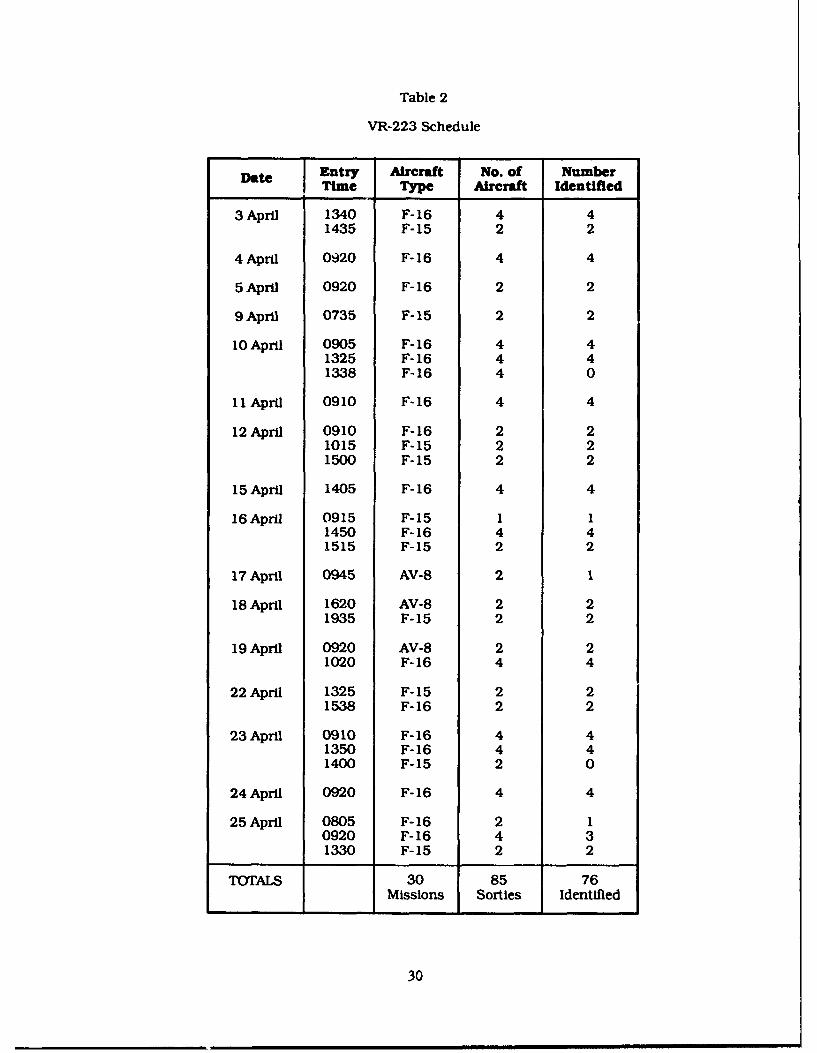
Table 2
VR-223 Schedule
Date Entry Aircraft No. of NumberITime Type Aircraft Identified
3 April 1340 F- 16 4 4
1435 F-15 2 2
4 April 0920 F- 16 4 4
5 April 0920 F- 16 2 2
9 April 0735 F- 15 2 2
10 April 0905 F- 16 4 41325 F- 16 4 41338 F-16 4 0
11 April 0910 F-16 4 4
12 April 0910 F-16 2 21015 F-15 2 21500 F-15 2 2
15 April 1405 F-16 4 4
16 April 0915 F-15 1 11450 F-16 4 41515 F-15 2 2
17 April 0945 AV-8 2 1
18 April 1620 AV-8 2 21935 F-15 2 2
19 April 0920 AV-8 2 21020 F-16 4 4
22 April 1325 F-15 2 21538 F-16 2 2
23 April 0910 F-16 4 41350 F-16 4 41400 F-15 2 0
24 April 0920 F- 16 4 4
25 April 0805 F- 16 2 10920 F- 16 4 31330 F-15 2 2
TOTALS 30 85 76Missions Sorties Identified
30
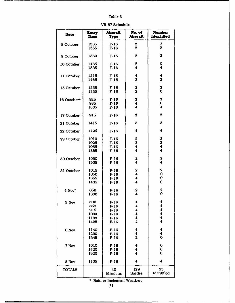
Table 3
VR-87 Schedule
Date Entry Aircraft No. of NumberTim" Type Aircraft Identified
8 October 1335 F-16 2 21555 F-16 2 2
9 October 1530 F-16 2 2
10 October 1435 F- 16 2 01535 F-16 4 4
11 October 1215 F-16 4 41455 F-16 2 2
15 October 1235 F-16 2 21335 F-16 2 0
16 October* 925 F-16 2 2935 F-16 4 01335 F-16 4 4
17 October 915 F-16 2 2
21 October 1415 F-16 3 3
22 October 1725 F-16 4 4
29 October 1010 F-16 2 21025 F-16 2 21055 F-16 4 41355 F-16 4 4
30 October 1050 F-16 2 21535 F-16 4 4
31 October 1015 F-16 2 21050 F-16 4 01355 F-16 4 01435 F-16 4 0
4 Nov* 850 F-16 2 21330 F-16 4 0
5 Nov 800 F-16 4 4853 F-16 4 4915 F-16 4 4
1034 F-16 4 41133 F-16 4 41425 F-16 4 4
6 Nov 1140 F-16 4 41200 F-16 4 41545 F-16 2 0
7 Nov 1010 F-16 4 01420 F-16 4 01520 F-16 4 0
8 Nov 1135 F-16 4 4
TOTALS 40 129 95Missions Sorties Identified
* Rain or Inclement Weather.
31
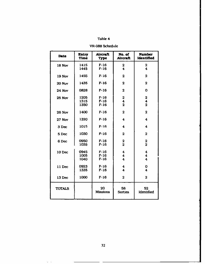
Table 4
VR-088 Schedule
Date Entry Aircraft No. of NumberTime Type Aircraft Identified
18 Nov 1415 F-16 2 21445 F-16 4 4
19 Nov 1455 F- 16 2 2
20 Nov 1435 F- 16 2 2
24 Nov 0828 F- 16 2 0
25 Nov 1205 F- 16 2 21315 F-16 4 41350 F-16 2 2
26 Nov 1400 F- 16 2 2
27 Nov 1320 F- 16 4 4
3 Dec 1015 F-16 4 4
5 Dec 1030 F-16 2 2
6 Dec 0950 F-16 2 21035 F-16 2 2
10 Dec 0945 F- 16 4 41005 F-16 4 41040 F- 16 4 4
11 Dec 0923 F-16 4 01335 F-16 4 4
13 Dec 1000 F- 16 2 2
TOTALS 20 58 52Missions Sorties Identified
32

Table 5
VR- 1074 Schedule
Date Time Aircraft No. of NumberT"e Aircraft Identified
3 February 1025 F- 15 4 40940 AV-8 2 01535 F- 15 2 21645 F- 15 2 2
4 February 0820 AV-8 2 20900 AV-8 2 20925 AV-8 2 21015 A-6 2 21030 AV-8 2 01415 A-6 1 01420 T-38 2 21515 A-6 2 21540 AV-8 2 01610 F- 15 4 41645 A-6 1 1
5 February 0945 AV-8 2 21100 A-6 2 21140 F- 15 2 21250 AV-8 2 21435 F- 15 2 21457 F- 15 2 21502 AV-8 2 21515 AV-8 2 21550 AV-8 2 21605 F- 15 4 4
6 February 0945 A-6 1 11035 F- 15 2 2
7 February 0835 "-8 2 01250 AV-8 1 1
8 February 1500 A-6 2 0
9 February No Schedule
10 February 1755 F- 15 2 21805 F- 15 2 21820 F- 15 2 0
11 February* 0815 F- 15 4 40925 AV-8 2 01135 AV-8 2 21251 F- 15 2 21300 F- 15 2 21725 F- 15 2 21735 F- 15 2 21800 F- 15 3 32037 F- 15 3 32100 F- 15 3 3
33
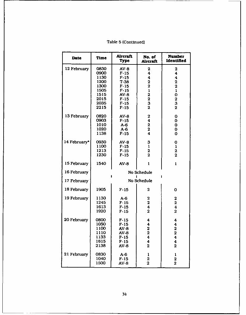
Table 5 (Continued)
Date Time Aircraft No. of NumberType Aircraft Identified
12 February 0830 AV-8 2 20900 F- 15 4 41130 F- 15 4 41200 T-38 2 21300 F- 15 2 21505 F- 15 1 11515 AV-8 2 02015 F-15 2 22035 F- 15 3 32215 F-15 2 2
13 February 0820 AV-8 2 00903 F- 15 4 01010 A-6 2 01020 A-6 2 01138 F-15 4 0
14 February* 0930 AV-8 3 01100 F-15 1 11213 F-15 2 21230 F-15 2 2
15 February 1540 AV-8 1 1
16 February No Schedule
17 February No Schedule
18 February 1905 F- 15 2 0
19 February 1130 A-6 2 21245 F-15 2 21613 F-15 4 41920 F-15 2 2
20 February 0800 F- 15 4 41050 F- 15 4 41100 AV-8 2 21110 AV-8 2 21133 F- 15 4 41615 F-15 4 42138 AV-8 2 2
21 February 0830 A-6 1 11040 F-15 2 21500 AV-8 2 2
34
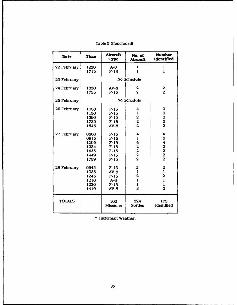
Table 5 (Concluded)
Date Time Aircraft No. of Number
Type Aircraft Identified
22 February 1230 A-6 1 1
1715 F-18 1 1
23 February No Schedule
24 February 1330 AV-8 2 21755 F-15 2 2
25 February No Sch--dule
26 February 1058 F-15 4 01130 F-15 1 01350 F- 15 2 01739 F-15 2 01545 AV-8 2 2
27 February 0800 F- 15 4 40915 F-15 1 01105 F-15 4 41334 F-15 2 21435 F-15 2 21449 F-15 2 21759 F-15 2 2
28 February 0945 F- 15 2 21035 AV-8 1 11245 F-15 2 21210 A-6 1 11220 F-15 1 11419 AV-8 3 0
TOTALS 100 224 175Missions Sorties Identified
Inclement Weather.
35

observed on 26 and 27 March. Notice that none of the eight missions scheduled
for these two days was detected by the monitors. Rain was also noted on the
afternoon of 20 March. A mission of two F- I6s was scheduled but not detected on
this day.
If the 9 missions which were not detected by the monitors and occurred on
days when inclement weather was noted are removed from the schedule, then a
total of 68 missions (150 sorties) were scheduled for the period. Of these. 31
sorties (about 20 percent) went undetected by the monitors. If all 19 missions of
which no sorties were detected are removed from the schedule, a total of 58
missions (127 sorties) were scheduled. Of these, only 6 sorties (about 5 percent)
went undetected.
In addition to the scheduled missions, 34 missions (consisting of 43 sorties)
were recorded by the noise monitors which did not appear on the schedule. Of
these 34 missions, 28 consisted of a single aircraft. Many of these unscheduled
missions were apparently A- 10s which were observed in the area.* The total
number used in the statistical analysis was 162 sorties contained in 83 missions:
the total of all detected scheduled missions, plus the unscheduled A- lOs.
4.2.2 VR-223. Arizona
Table 2 lists the schedule data for VR-223 for the measurement period of
3 April through 25 April 1991. A total of 30 missions were flown during this
period. Of these 30 missions, 17 were F-16s, 10 were F-15s and 3 were AV-8s.
These 30 missions constituted 85 sorties of which 76 sorties (about 90 percent)
were recorded by the monitors. Of the 9 sorties that went undetected, 6 sorties
were from missions where none of the aircraft were detected. As discussed
previously, it is unlikely that all aircraft in a mission could pass the monitors
undetected. It is more likely that these missions either did not fly or left the
route before reaching the measurement array. Another possibility is that the
undetected sorties flew over the eastern portion of the route which contained no
monitors. This part of the route was generally avoided by the aircraft due to the
mountainous terrain, and 'would have involved substantially higher altitude.
* A-10s fly at lower speeds, and therefore do not necessarily have to scheduleroute usage.
36
In addition to the scheduled flights. 26 missions (consisting of 39 sorties)
were measured which did not appear on the schedule. Again, these were
apparently A- Os. Of the 26 unscheduled missions, 17 consisted of a single sortie.
The total number used for the statistical analysis was 115 sorties contained in
56 missions, the total of detected scheduled missions plus detected unscheduled
missions.
4.2.3 VR-087. South Carolina
Table 3 lists the schedule data for VR-087 during the measurement period
of 8 October through 8 November 199 1. A total of 40 missions consisting of
129 sorties were scheduled during this period. All of the scheduled missions
were for F- 16 aircraft. Of the 129 scheduled sorties. 95 (or about 75 percent)
were detected by the noise monitors leaving 34 undetected sorties. All of the
undetected sorties were contained in missions which had no sorties detected. It
is reasonable to assume that most. if not all, of the undetected missions did not
cross the measurement array.
No unscheduled missions were measured by the monitors on this route.
The total sortie count used in the statistical analysis was 95 contained in
40 missions.
4.2.4 VR-088. South Carolina
Table 4 contains the schedule data for VR-088 through the measurement
period of 18 November to 13 December 1991. A total of 20 missions containing
58 sorties of F- 16s were scheduled for the period. Of these 58 scheduled sorties,
52 (about 90 percent) were measured by the monitors. All of the undetected
sorties were from missions with no detected aircraft. These missions were
probably canceled or exited the route before reaching the measurement array.
No unscheduled missions were recorded on this route. The total sortie
count used in the statistical analysis was 52 contained in 18 missions.
37
4.2.5 VR- 1074. North Carolina
Table 5 lists the schedule data for VR- 1074 through the measurement
period of 3 February to 28 February 1992. A total of 100 missions containing 224
sorties were scheduled over the period. Most of these aircraft were F- 15s and
AV-8s. Of the 224 sorties, 175 (about 78 percent) were detected by the monitors.
All of the undetected sorties were scheduled within missions where no aircraft
were detected. These missions probably left the route before reaching the
monitors, flew around the monitors, or were canceled due to weather. Morning
fog was noted in the area on the 11 and 14 February and heavy rain was reported
in the area most of the day on 26 February. These days of inclement weather
account for 11 undetected, scheduled sorties. Removing these from the schedule
makes the detection rate 85 percent.
In addition. 15 missions consisting of 25 sorties were detected which didnot appear on the schedule. The total number used for the statistical analysis was
200 sorties contained in 93 missions.
4.3 MTR Measurement Results
The discussion of the measurement results revolves around several figures
which require some introduction. There are four figures for each of the five routes.
Figures 13 through 16 correspond to VR- 1220, and consist of the following:
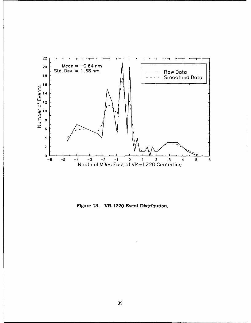
"Figure 13 shows the distribution of sorties recorded by the measure-
ment arrays. The positions of individual sorties were assumed to be over
the monitor site which recorded the maximum level. In each figure a
plot of the raw data and smoothed data are shlown. The smoothed data
was calculated from the weighted average of the site and the two sites
adjacent to it. The site was weighted 50 percent and the two adjacent
sites were weighted 25 percent. Since the total number of events at any
particular site were statistically low, the smoothed distribution is
probably a better representation of the data.
"* Figure 14 shows the cumulative probability distribution of position. In
the case of a perfectly Gaussian distribution this plot would appear as a
38
22
20 Mean = -0.64 nmStd. Dev. = 1.68 nm Raw Data
18 ... - Smoothed Data
164-
(D 14
LU_"-.120
_Q)1
E 8z
6
4
2
0-6 -5 -4 -3 -2 -1 0 1 2 3 4 6
Nautical Miles East of VR-1 220 Centerline
Figure 13. VR- 1220 Event Distribution.
39
ge•
msI
90 A----B'•)* --. ..
80 k . . . . .... .
70
3040
20l-O --
10
0.01 .. ...
•6 -5 4 -3 -2 -1 0 1 2 3 4 5 6
Nautical Mkgs East of VR-1220 Centerline
Figure 14. VR- 1220 Event Cumulative Probability Distribution.
40
110
100
90{/)< 80
0 70
o 60xLLJ 5
50
- 40
E 30
Z 20
10
0 I * I * I I I I * I * I * I *-6 -5 -4 -3 -2 -1 0 1 2 3 4 5 6
Nautical Miles East of VR-1 220 Centerline
Figure 15. VR- 1220 Total Events at Each Site.
41

0m 40 1 F F
Total Avg. =106 dBCD30 Scheduled Avg. = 1 06 dB
Cn Unscheduled Avg. = 1 02 dB
>20Lii
%ý_ Scheduled0 UnscheduledCD 0
Ez 0
80 90 100 110 120Sound Exposure Level, dB
(a) Distribution of Highest SEL for Each Event.
M 0
30 TtaI~g.=l~dB ____Scheduled
CD 3 Scheduled Avg. = 1 04 dBUnceudV) -Unscheduled Avg. =98dB
C
>20LuJ
0
0'10
Ez 0
80 90 100 110 120A-Weighted Sound Level, dB
(b) Distribution of Highest Maximum Level for Each Event.
Figure 16. Distribution of Event Sound Levels, VR- 1220.
42
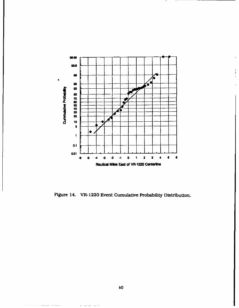
straight line. Each of these plots contains the individual site data points
along with an ideal Gaussian straight line for comparison.
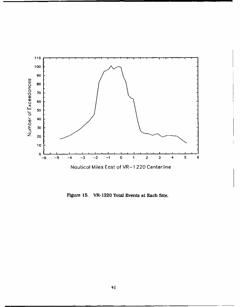
" Figure 15 shows the total number of events recorded at each site. This
represents the number of aircraft which exceeded the monitor
threshold level of 65 to 70 dB during the four-week measurement period.
" Figure 16 shows the distributions of the measured sound exposure level
and maximum level. These are the maximum for each event, and
represent noise levels occurring within half the monitor spacing of the
flight track. In addition, the measured levels are split between
scheduled and unscheduled events.
4.3.1 VR- 1220 Measurement Results
The distribution obtained for VR-1220, shown in Figure 13. has a mean of
-0.64 nautical mile and a standard deviation of 1.68 nautical miles. The offset of
the distribution toward the west may be due to higher terrain east of the route
centerline. The aircraft tended to fly to the west, avoiding this higher terrain.
The cumulative probability distribution for VR- 1220 is shown in Figure 14. If the
data distribution were perfectly Gaussian it would appear as a straight line on the
probability plot. A line has been drawn on Figure 14 corresponding to a Gaussian
distribution having a mean of -0.64 nautical mile and a standard deviation of
1.68 nautical miles. As is evident, the actual data follows the straight line fairly
well with some deviation just east of the route centerline.
The total number of events recorded at each site are shown in Figure 15.
These include all exceedances (i.e., sound levels above the threshold of 65 to
70 dB) associated with aircraft overflights, not just the maximum.
Figure 16(a) shows the distribution of Sound Exposure Levels per 2 dB
increment for each detected sortie. This is a count of the number of events whose
event-center SEL fell within each 2 dB bin. For example, for VR- 1220, 32 of the
measured events had a minimum SEL between i06 dB and 108 dB. The energy-
average sound level for this distribution is 105.6 dB. Given the type of aircraft on
the route and their proportionate number of operations, the average operating
altitude of the aircraft can be estimated. For example. on VR- 1220 about two-
43
altitude of the aircraft can be estimated. For example, on VR- 1220 about two-
thirds of the operations were F- 16s and the remaining one-third were F- 15s. It is
known that an F- 16 flying at 500 feet under typical MTR flight conditions
produces an SEL of 102 dB on the ground. Similarly, an F- 15 produces an SEL of
105 dB. Therefore, if all of the aircraft on VR- 1220 flew at 500 feet they would
produce an energy-average SEL of 103 dB. Since the energy-average SEL for the
VR- 1220 measurements was 105.6 dB, it can be inferred that the aircraft were
operating at an average altitude of about 300 feet.
The distribution in Figure 16(a) is also split between scheduled and
unscheduled events. The energy average was 106 dB for scheduled events and
102 dB for unscheduled events. The significantly lower levels associated with the
unscheduled events are due to A- Os which produce relatively low noise levels.
A similar plot is shown in Figure 16(b) for the maximum level associated
with each event. The energy average maximum level on VR- 1220 was 101.6 dB.
As before, the average level of unscheduled events is significantly lower than for
scheduled events.
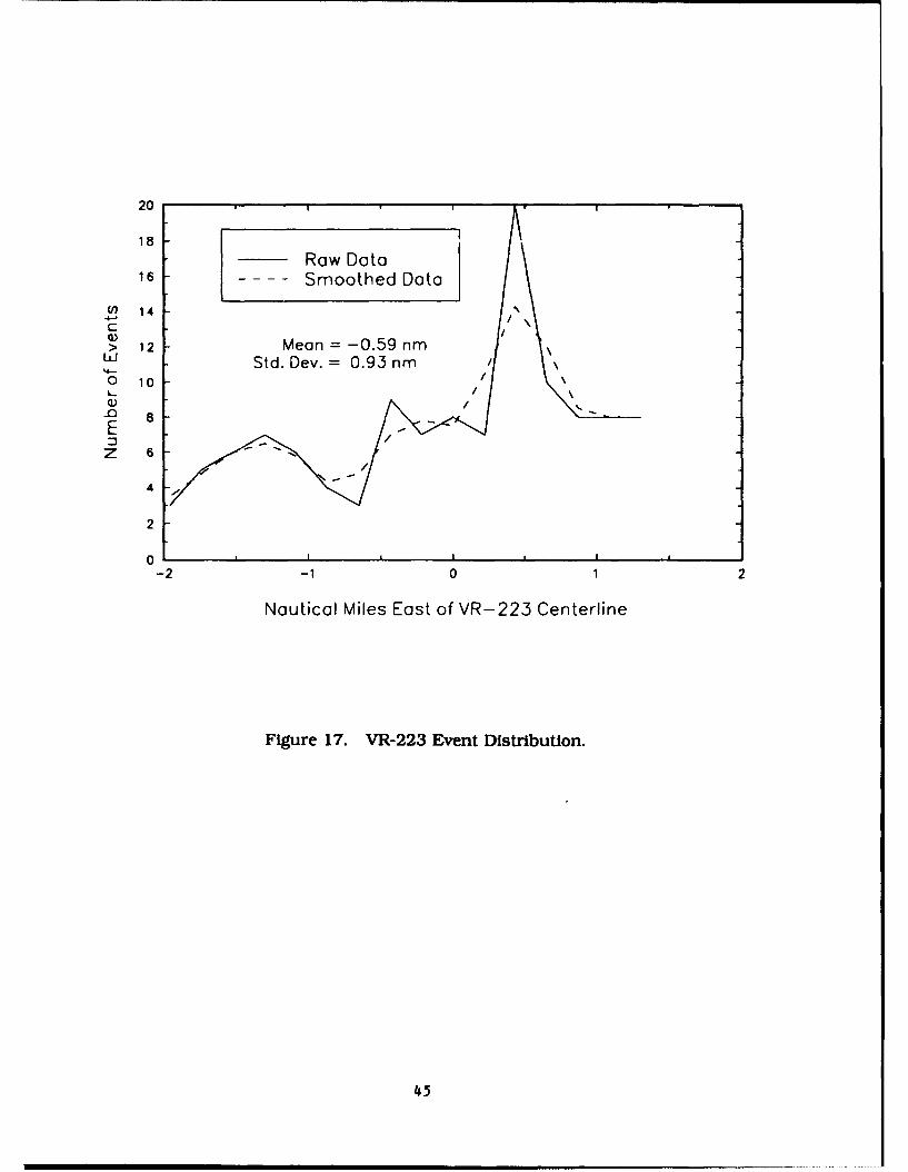
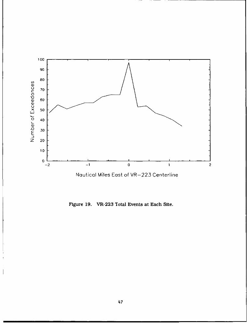
4.3.2 VR-223 Measurement Results
The distribution obtained for VR-223. shown in Figure 17, has a mean of
-0.59 nautical mile and a standard deviation of 0.93 nautical miles. The offset of
the mean is due to Tabletop Mountain under the eastern part of the route, which
the aircraft had to fly around. The cumulative probability distribution for VR-223
is shown in Figure 18. The data obtained follows the straight line of an ideal
normal distribution fairly well. The total exceedances measured at each site are
shown in Figure 19.
Unlike VR-1220. where all operations were well contained within the route
boundaries, operations on VR-223 extended to the western edge. It appears that
the three miles available at this choke point is close to the minimum necessary for
this type of route. The standard deviation is the smallest measured on any
TAC route.
Figure 20(a) shows the distribution of SELs per 2 dB for each measured
event. The energy average associated with these measurements is 105.1 dB. This
44!
20
18
Raw Data16 - Smoothed Data
(n 14C
> 12 Mean = -0.59 nm• Std. Dev. = 0.93 nm 70 10
a)ýO 8E -
z 6
4
2
0-2 -1 0 1
Nautical Miles East of VR-223 Centerline
Figure 17. VR-223 Event Distribution.
45

95
so ---- - --- . -. -.. ...-... .... -... ....-........ -. - .- - - -...-...................
0 . ..... .
30. ...................... ....... ..................... .. ................. .................. ..................... .............. .. ....... . ..
-2 -1 0 1 2
Nautical MHes East of VR-223 Centealine
Figure 18. VR-223 Event Cumulative Probability Distribution.
46
100
90
80(D0 70C,0
-aJ• 60
x 50
0 40
30
EZ 20
10
0-2 -1 0 1 2
Nautical Miles East of VR-223 Centerline
Figure 19. VR-223 Total Events at Each Site.
47

M 4 0 i j u * * i , , , ,
Total Avg. = 105 dB30 Scheduled Avg. = 1 06 dB
(n Unscheduled Avg. = 102 dBC
> 20w%- - Scheduledo Unscheduled
010 _ _ _ _ _ _
Ez 0
80 90 100 110 120Sound Exposure Level, dB
(a) Distribution of Highest SEL for Each Event.
" 40
Total Avg. = 101 dB'D 30 Scheduled Avg. = 1 02 dB _ Scheduled
(n Unscheduled Avg. 98 dB Unscheduled
> 20ILi
0L..
0)10
E
80 90 100 110 120A-Weighted Sound Level, dB
(b) Distribution of Highest Maximum Level for Each Event.
Figure 20. Distribution of Event Sound Levels. VR-223.
48

translates into an average altitude of operation of 400 feet. Figure 20(b) is the
distribution of maximum levels per 2 dB which has an energy average of 101.3 dB.
As with the previous MTR. the average levels for unscheduled events aremuch lower than the scheduled event average. This is once again due to A-10
activity.
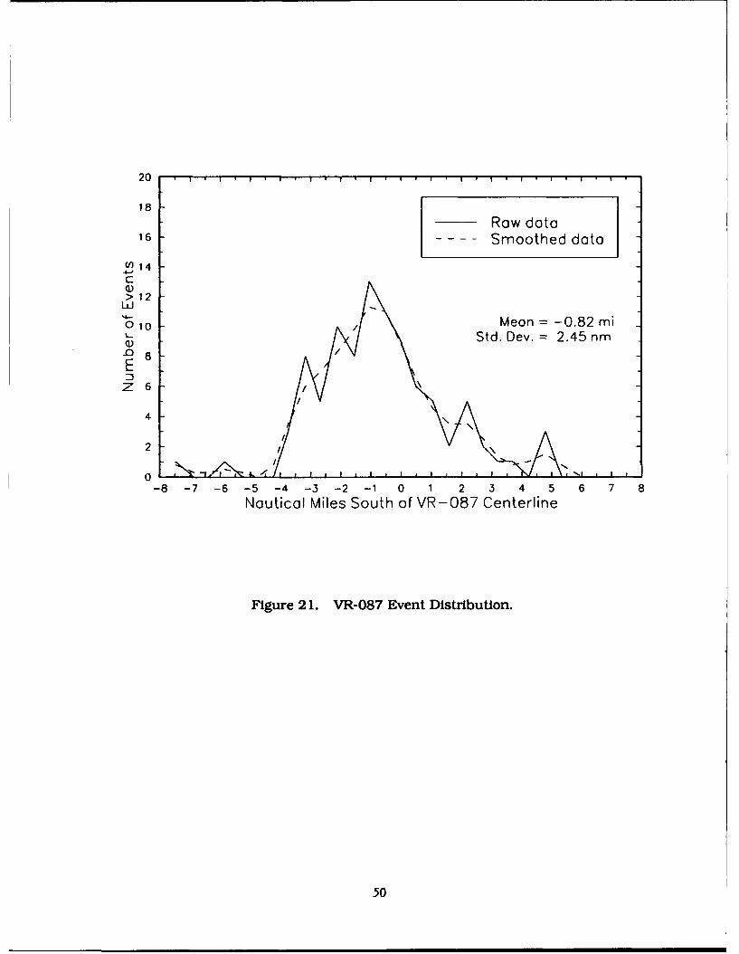
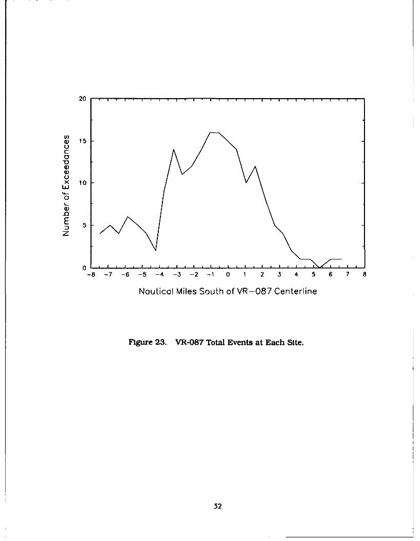
4.3.3 VR-087 Measurement Results
The distribution for VR-087, shown in Figure 2 1. has a mean of -0.82 nauti-
cal mile and a standard deviation of 2.45 nautical miles. The offset of the mean, in
this case. may be due to the location of the 1-95/Route 527 intersection 1.3 nauti-
cal miles north of the centerline. The aircraft operating on the route may use thisas a navigation landmark, thus shifting the center of operations toward it. The
cumulative probability distribution for VR-087 is shown in Figure 22. The data
follows the straight line of the ideal normal distribution fairly well except near thenorth end of the route. The total exceedances measured at each site are show in
Figure 23.
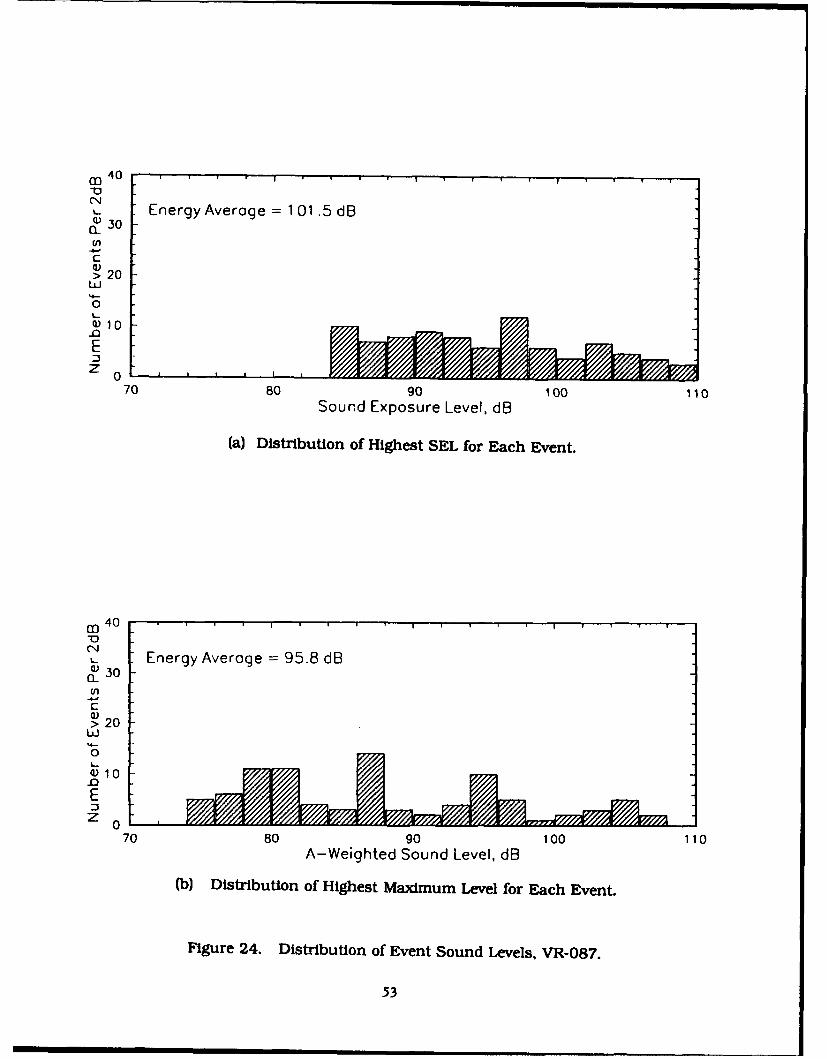
The distribution of sound exposure levels for VR-087 is shown in Fig-ure 24(a). The energy average for this distribution is 101.5 dB which coincideswith an average altitude of operation of 600 feet. The distribution of event
maximum levels per 2 dB is shown In Figure 24(b). The corresponding energy
average is 95.8 dB.
4.3.4 VR-088 Measurement Results
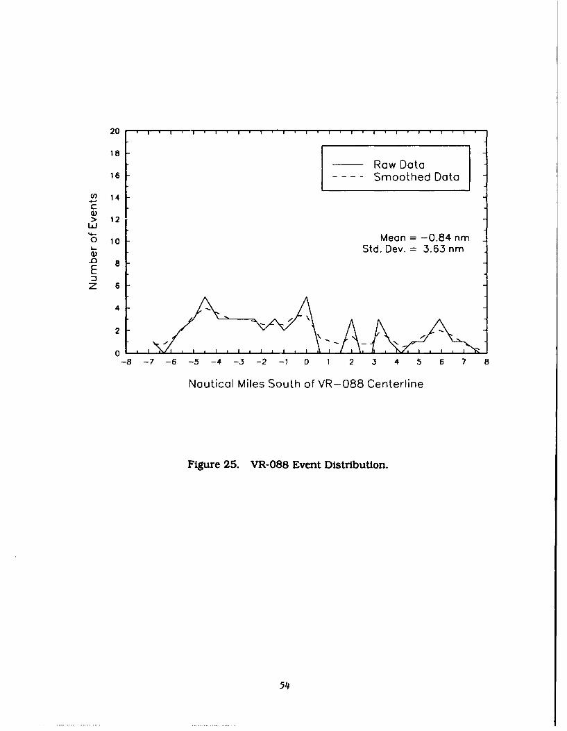
The distribution of events along VR-088, shown in Figure 25, has a mean of-0.84 nautical mile and a standard deviation of 3.63 nautical miles. Notice that thedata in Figure 25 does not appear normal in shape, but appears to be uniform
across the route. This is probably due to the low number of events recorded onthe route, and the reliability of the standard deviation is questionable. The offset
of the mean may be due to the presence of a small town directly under the route
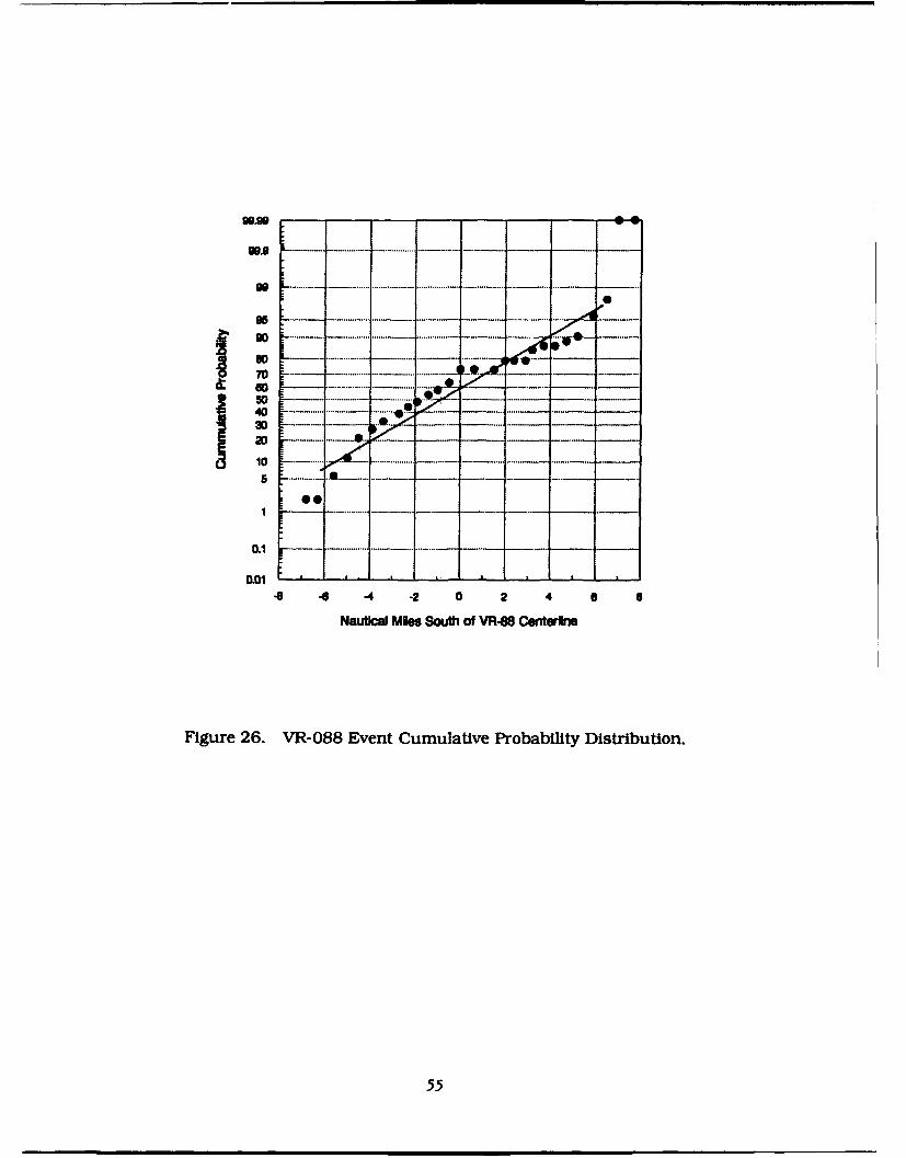
centerline along the measurement array which the aircraft avoided to the north.The cumulative probability distribution for VR-088 is shown in Figure 26. Even
though the event distribution plot in Figure 25 does not appear Gaussian, the data
49
20
18
Raw data16 Smoothed data
4 f)14
>12bJJ
00 oMeon = -0.82 miStd. Dev. = 2.45 nm
_ 8EZ6
4
2/
-8 -7 -6 -5 -4 -3 -2 -1 0 1 2 3 4 5 6 7 8Nautical Miles South of VR-087 Centerline
Figure 21. VR-087 Event Distribution.
50

99.9 - --------- ---------- ------ - -.. ...---
99.9 ...... ... _9o
90
30. . . ... .. ... . . .
-6 - -4 -2 0 2 4 6--
Nautical Mises South of VR-87 Cuiterlins
Figure 22. VR-087 Event Cumulative Probability Distribution.
051
20 . 1 1
S15c
%I)
0
E 5
-o
Z
0
-8 -7 -6 -5 -4 -3 -2 -1 0 o
Nauticol Miles South of VR-087 Centerline
Figure 23. VR-087 Total Events at Each Site.
52
"40
Energy Average = 101 .5 dBS30
> 20lUJ%4.-0L.
Q) 10-oEz 0
70 80 90 100 110Sound Exposure Level, dB
(a) Distribution of Highest SEL for Each Event.
(G 40
30 Energy Average = 95.8 dBS30
C:0f)
> 20
0
Q) 1o
Ez o
70 80 90 100 110A-Weighted Sound Level, dB
(b) Distribution of Highest Maximum Level for Each Event.
Figure 24. Distribution of Event Sound Levels, VR-087.
53
20
18Raw Data
16 - - - - Smoothed Data
4-14
c
> 124-0 10 Mean = -0.84 nm
Std. Dev. = 3.63 nm
_o 8Ez 6
4
2
-8 -7 -6 -5 -4 -3 -2 -7 0 1 2 3 4 5 6 7 8
Nautical Miles South of VR-088 Centerline
Figure 25. VR-088 Event Distribution.
54
S.m. - -. -2- 2 4- --- '
so
955
50 -...----.--. .-
...... ... ......
10. .................
0.01 -- - --- --- L •
-8 -0 -4 -2 0 2 4 a
Nautica Mles South of VR-88 Cerderinm
Figure 26. VR-088 Event Cumulative Probability Distribution.
55
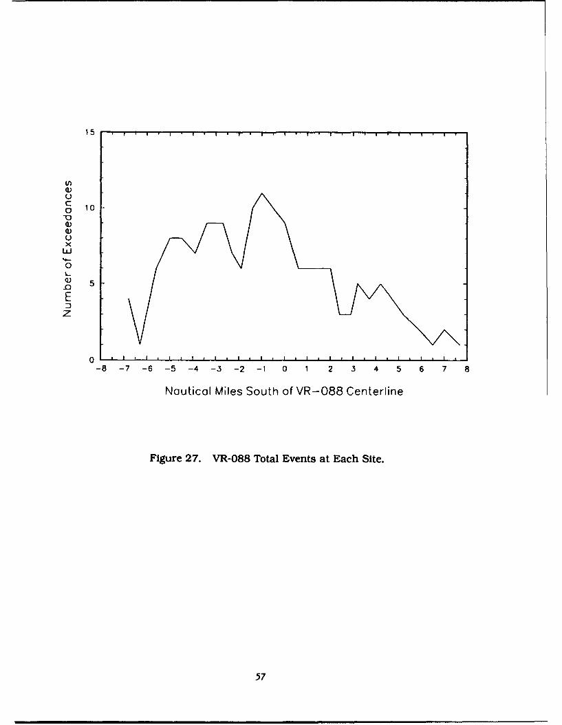
does follow the ideal normal distribution straight line over most of the central partof the route. The total number of exceedances measured at each site is shown inFigure 27.
The distribution of event SEL per 2 dB is shown in Figure 28(a). Thisdistribution has an energy average of 101.9 dB. Since all aircraft operating alongVR-088 were F- 16s, this corresponds to an average altitude of operation of500 feet. Figure 28(b) shows the distribution of event maximum levels per 2 dBincrement. This distribution has an energy average of 97.1 dB.
4.3.5 VR-1074 Measurement Results
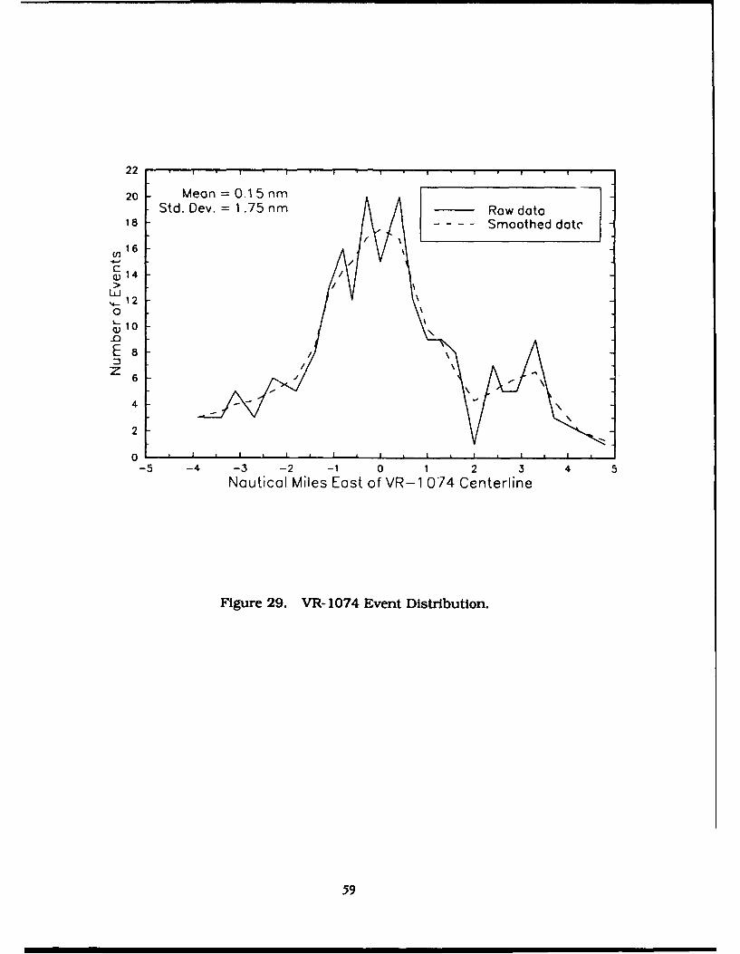
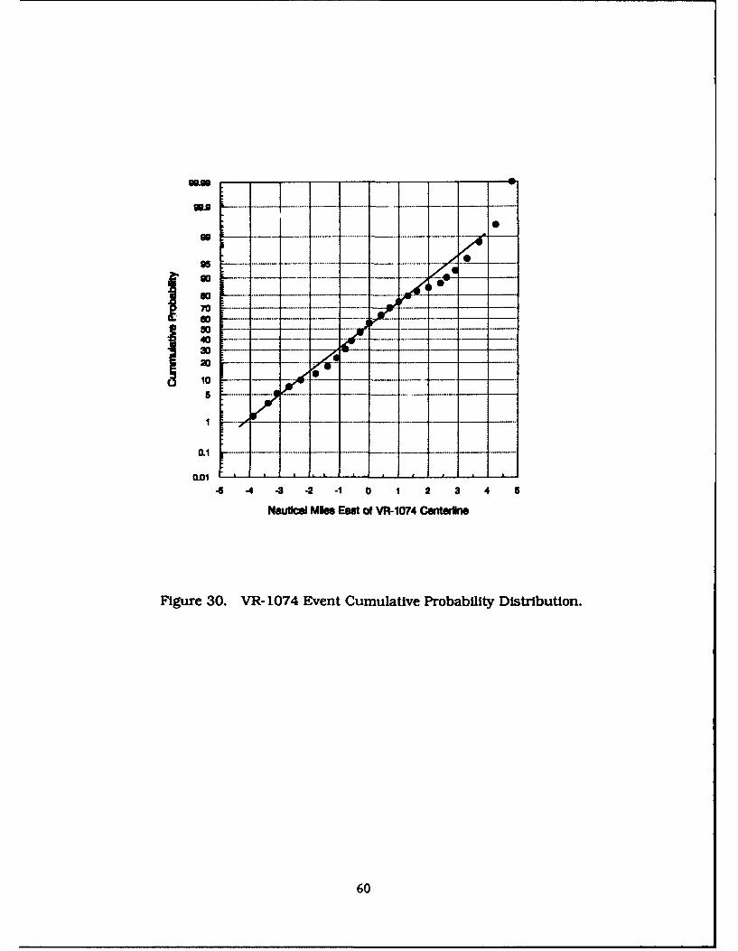
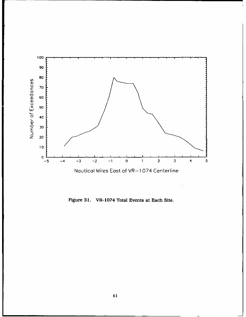
The event distribution on VR- 1074 as shown in Figure 29 has a mean of0.15 nm and a standard deviation of 1.75 nm. Although the offset of the distri-bution mean is small, it is consistent with the description of operations providedby the scheduling officer at Seymore-Johnson AFB. The presence of two radiotowers near the measurement array on the western side of the route forcedoperations east of the route centerline. The cumulative probability distribution forVR- 1074 measurements is shown in Figure 30. The data follows the ideal normaldistribution straight line extremely well. Figure 30 contains the total exceedancesmeasured at each site.
The distribution of event SEL per 2 dB increment is shown in Figure 32(a).This distribution has an energy average of 108.2 dB. This corresponds to anaverage altitude of operation of 500 feet for the proportionate number of F- 15s.AV-8s. and A-6s operating on the route. Figure 32(b) shows the distribution ofevent maximum levels per 2 dB interval. This distribution has an energy averageof 105.2 dB.
The distributions for scheduled and unscheduled events are split inFigures 32(a) and (b). As before, the average levels for unscheduled events arelower than those for scheduled events.
4.4 Noise Levels and ROUTEMAP Comparison
The primary purpose of this study is to verify and/or improve the currentversion of the ROUTEMAP noise modeling program. It has already been
56
15
V)
Co 10
a.)(-)x
LIJ
0
w 5l-0
EZ)z
0 * I * I i ! I . I . I , I * I , I I , I *
-8 -7 -6 -5 -4 -3 -2 -1 0 1 2 3 4 5 6 7 8
Nautical Miles South of VR-088 Centerline
Figure 27. VR-088 Total Events at Each Site.
57

40
30 Energy Averoge = 101 .9 dB•)30
C,C
> 20Li
0L_
0) 10
Ez 0 Rai•,///
70 80 90 100 110Sound Exposure Level, dB
(a) Distribution of Highest SEL for Each Event.
40 . , .
CO%
Energy Averoge = 97.1 dB30
V)
> 20-i,
0
a) 10-0
0 L7 &o .
70 80 90 100 110A-Weighted Sound Level, dB
(b) Distribution of Highest Maximum Level for Each Event.
Figure 28. Distribution of Event Sound Levels. VR-088.
58
22 , I • ,
20 Mean = 0.1 5 nmStd. Dev. = 1.75 nm Row data
18/" / - -Smoothed datc
(n16/
c14
LUJk4-12
0
E o
0 * I I * I * I I I * I
-5 -4 -3 -2 -1 0 1 2 3 4Nauticol Miles East of VR-1 074 Centerline
Figure 29. VR- 1074 Event Distribution.
59
700
10
5
M1.
-5 -4 -3 -2 -1 0 1 2 3 4
Ndutcal Min Eas of VR-1074 C- ter
Figure 30. VR- 1074 Event Cumulative Probability Distribution.
60
100
90
80
cnC,,
0-o• 60
x 50LuI0 40
F 30
Z 20
10
0
-5 -4 -3 -2 -1 0 1 2 3 4 5
Nautical Miles East of VR-1 074 Centerline
Figure 3 1. VR- 1074 Total Events at Each Site.
61

O 40
-oTotol Avg. = 108 dB
30 Scheduled Avg. = 1 09 dBUnscheduled Avg. = 1 05 dB
C20> 20
0-750= Scheduledo Unscheduled
0)10 _ _ _ _ _ _ _ _
Ez o
70 80 90 100 110 120Sound Exposure Level, dB
(a) Distribution of Highest SEL for Each Event.
m 40
Totol Avg. =105 dB _____ Scheduled30 P~•KX•Unscheduled30 Scheduled Avg. = 1 06 dB
E Unscheduled Avg. = 1 02 dBc
> 20w'4-
0
010
Ez o
70 80 90 100 110 120A-Weighted Sound Level, dB
(b) Distribution of Highest Maximum Level for Each Event.
Figure 32. Distribution of Event Sound Levels, VR- 1074.
62
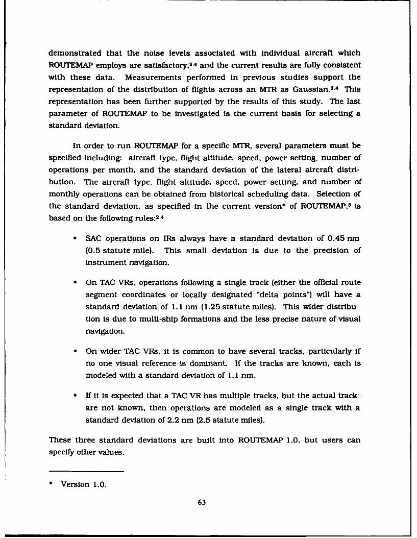
demonstrated that the noise levels associated with individual aircraft which
ROUTEMAP employs are satisfactory.2.4 and the current results are fully consistent
with these data. Measurements performed in previous studies support therepresentation of the distribution of flights across an MTR as Gaussian. 2.4 This
representation has been further supported by the results of this study. The last
parameter of ROUTEMAP to be investigated is the current basis for selecting astandard deviation.
In order to run ROUTEMAP for a specific MTR. several parameters must bespecified including: aircraft type. flight altitude, speed, power setting, number ofoperations per month, and the standard deviation of the lateral aircraft distri-
bution. The aircraft type, flight altitude, speed, power setting. and number ofmonthly operations can be obtained from historical scheduling data. Selection of
the standard deviation, as specified in the current version* of ROUTEMAP, 5 is
based on the following rules:2.4
" SAC operations on IRs always have a standard deviation of 0.45 nm
(0.5 statute mile). This small deviation is due to the precision of
instrument navigation.
" On TAC VRs. operations following a single track (either the official route
segment coordinates or locally designated "delta points") will have a
standard deviation of 1.1 nm (1.25 statute miles). This wider distribu-
tion is due to multi-ship formations and the less precise nature of visual
navigation.
" On wider TAC VRs, it is common to have several tracks, particularly ifno one visual reference is dominant. If the tracks are known, each is
modeled with a standard deviation of 1.1 nm.
" If it Is expected that a TAC VR has multiple tracks, but the actual track,
are not known, then operations are modeled as a single track with a
standard deviation of 2.2 nm (2.5 statute miles).
These three standard deviations are built into ROUTEMAP 1.0, but users can
specify other values.
* Version 1.0.
63
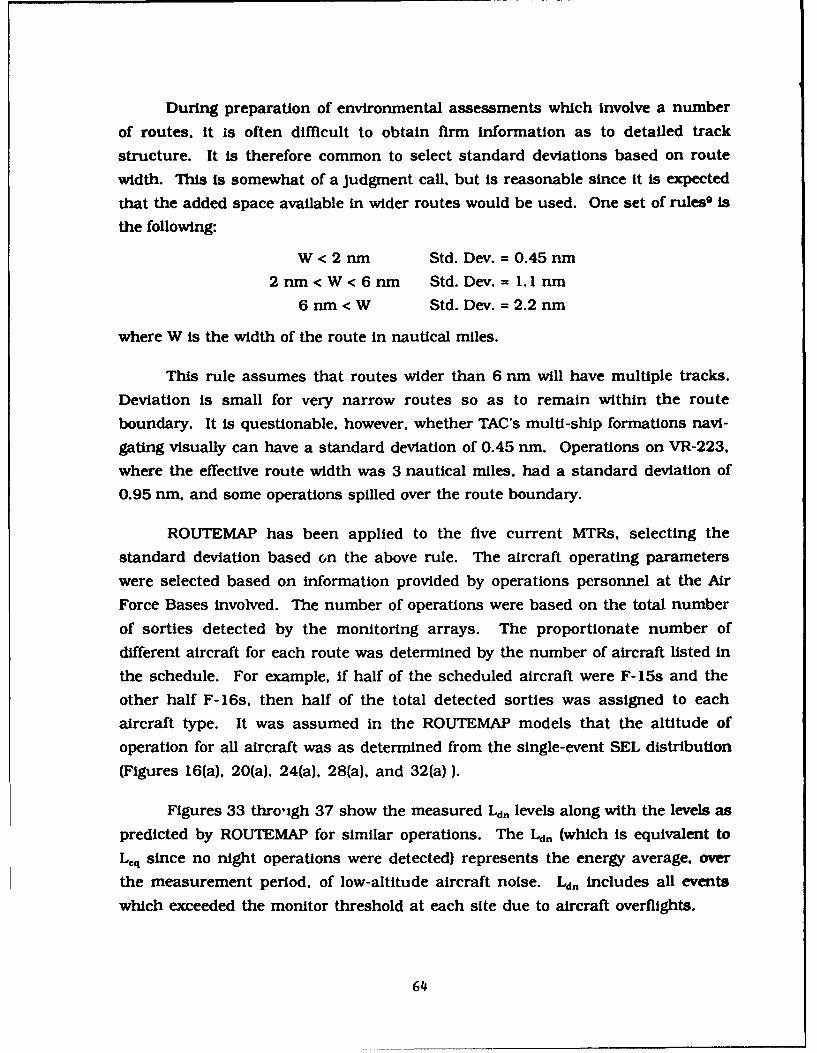
During preparation of environmental assessments which involve a number
of routes, it is often difficult to obtain firm information as to detailed track
structure. It is therefore common to select standard deviations based on route
width. This is somewhat of a judgment call, but is reasonable since it is expected
that the added space available in wider routes would be used. One set of rules9 is
the following:
W < 2 nm Std. Dev. = 0.45 nm
2 nm < W < 6 nm Std. Dev. = 1.1 nm
6 nm < W Std. Dev. = 2.2 nm
where W is the width of the route in nautical miles.
This rule assumes that routes wider than 6 nm will have multiple tracks.
Deviation is small for very narrow routes so as to remain within the route
boundary. It is questionable, however, whether TAC's multi-ship formations navi-
gating visually can have a standard deviation of 0.45 nm. Operations on VR-223.
where the effective route width was 3 nautical miles, had a standard deviation of
0.95 nm, and some operations spilled over the route boundary.
ROUTEMAP has been applied to the five current MTRs, selecting the
standard deviation based on the above rule. The aircraft operating parameters
were selected based on information provided by operations personnel at the Air
Force Bases involved. The number of operations were based on the total number
of sorties detected by the monitoring arrays. The proportionate number of
different aircraft for each route was determined by the number of aircraft listed in
the schedule. For example, if half of the scheduled aircraft were F- 15s and the
other half F- 16s. then half of the total detected sorties was assigned to each
aircraft type. It was assumed in the ROUTEMAP models that the altitude of
operation for all aircraft was as determined from the single-event SEL distribution
(Figures 16(a), 20(a). 24(a). 28(a), and 32(a)).
Figures 33 throuigh 37 show the measured Ldn levels along with the levels as
predicted by ROUTEMAP for similar operations. The Ld, (which is equivalent to
Leq since no night operations were detected) represents the energy average, over
the measurement period, of low-altitude aircraft noise. Ld, includes all events
which exceeded the monitor threshold at each site due to aircraft overflights.
64
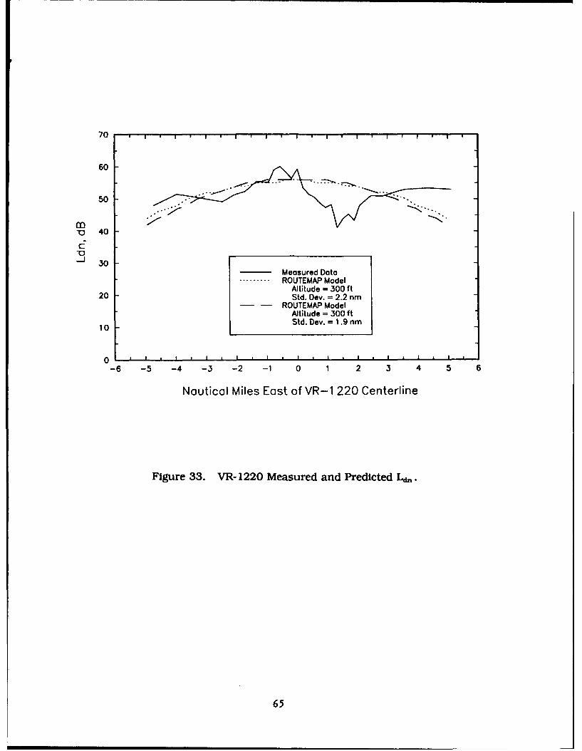
70 I
60
50
"0240
-j 30Measured DataROUTEMAP Model
Altitude = 300 ft20 Std. Dev. = 2.2 nm
ROUTEMAP ModelAltitude = 300 ft
10 Std. Dev. = 1.9 nm
100 * * I . I * I i , I , i * I * I * I *
-6 -5 -4 -3 -2 -1 0 1 2 3 4 5 6
Nautical Miles East of VR-1 220 Centerline
Figure 33. VR- 1220 Measured and Predicted Ld.
65
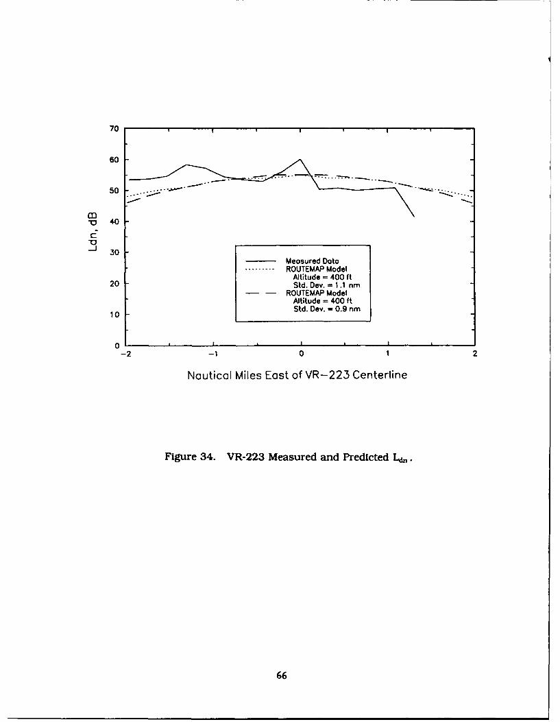
70
60
50
m- 40
-o _ _ _ _ _ _ _ _
J 30Measured DataROUTEMAP Model
Altitude = 400 ft20 Std. Dev. = 1.1 nm
ROUTEMAP ModelAltitude = 400 ft
10 Std. Dev. = 0.9 nm
10
-2 -1 0 1 2
Nautical Miles East of VR-223 Centerline
Figure 34. VR-223 Measured and Predicted Ld.
66
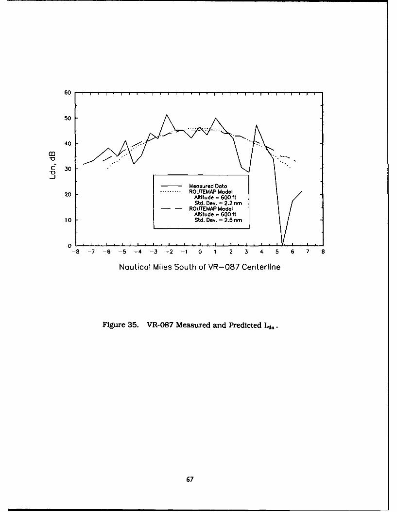
60
50
40
C" 30 .""._J
Measured Data
20 ROUTEMAP ModelAltitude = 600 ftStd. Dev. = 2.2 nm
ROUTEMAP ModelAltitude = 600 ft
10 Std. Dev. - 2.5 nm
0-8 -7 -6 -5 -4 -3 -2 -1 0 1 2 3 4 5 6 7
Nauticol Miles South of VR-087 Centerline
Figure 35. VR-087 Measured and Predicted Ld,.
67
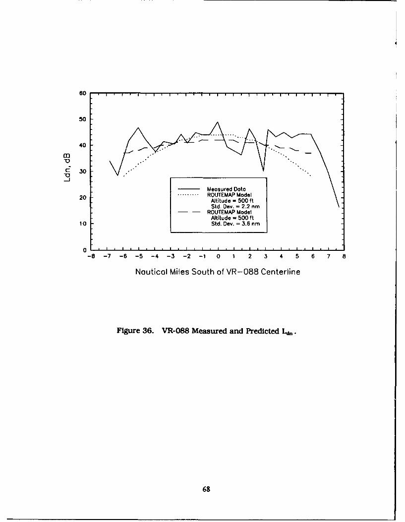
60
50
40
S30._J
Measured Data20......... ROUTEMAP Model
Altitude = 500 ftStd. Dev. = 2.2 nm
ROUTEMAP ModelAltitude = 500 ft
10 Std. Dev. = 3.6 nm
0 * , I , I * I * I * I , I I I i I * I , I * I *
-8 -7 -6 -5 -4 -3 -2 -1 0 1 2 3 4 5 6 7 8
Nouticol Miles South of VR-088 Centerline
Figure 36. VR-088 Measured and Predicted Ld..
68
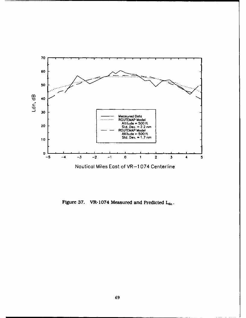
70
60
50 -•"
m- 40
-J 30
Measured DataROUTEMAP Model
Altitude - 500 ft20 Std. Dev. = 2.2 nm
ROUTEMAP ModelAltitude = 500 ft
10 Std. Dev. = 1.7 nm
0 , * I * I * I * I * I * I * I *-5 -4 -3 -2 -1 0 1 2 3 4 5
Nouticol Miles East of VR-1 074 Centerline
Figure 37. VR- 1074 Measured and Predicted Ld,.
69
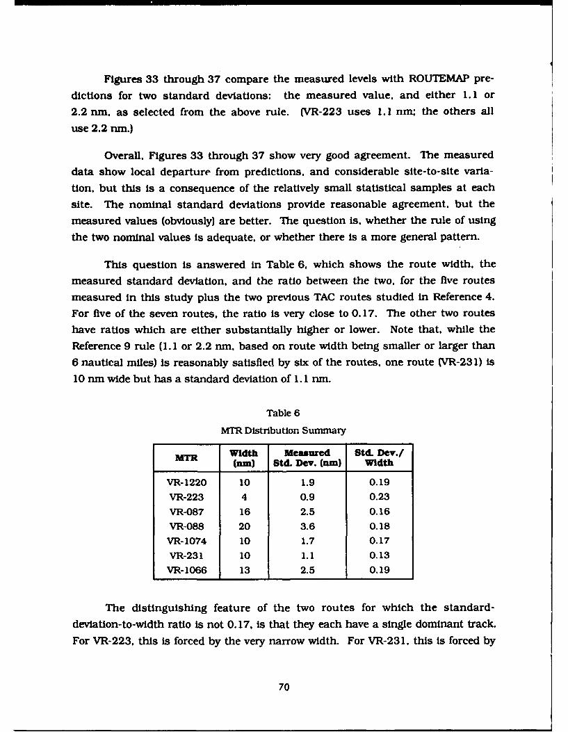
Figures 33 through 37 compare the measured levels with ROUTEMAP pre-
dictions for two standard deviations: the measured value, and either 1. 1 or
2.2 nm. as selected from the above rule. (VR-223 uses 1. 1 nm: the others all
use 2.2 rum.)
Overall. Figures 33 through 37 show very good agreement. The measured
data show local departure from predictions, and considerable site-to-site varia-
tion, but this is a consequence of the relatively small statistical samples at each
site. The nominal standard deviations provide reasonable agreement. but the
measured values (obviously) are better. The question is. whether the rule of using
the two nominal values is adequate. or whether there is a more general pattern.
This question is answered in Table 6. which shows the route width, the
measured standard deviation, and the ratio between the two, for the five routes
measured in this study plus the two previous TAC routes studied in Reference 4.
For five of the seven routes, the ratio is very close to 0.17. The other two routes
have ratios which are either substantially higher or lower. Note that, while the
Reference 9 rule (I. 1 or 2.2 rum, based on route width being smaller or larger than
6 nautical miles) is reasonably satisfied by six of the routes, one route (VR-231) is
10 nm wide but has a standard deviation of 1.1 nm.
Table 6
MTR Distribution Summary
MTR Width Measured Std. Dev./
(nm) Std. Dev. (nm) Width
VR-1220 10 1.9 0.19
VR-223 4 0.9 0.23
VR-087 16 2.5 0.16
VR-088 20 3.6 0.18
VR-1074 10 1.7 0.17
VR-231 10 1.1 0.13VR-1066 13 2.5 0.19
The distinguishing feature of the two routes for which the standard-
deviation-to-width ratio is not 0.17, is that they each have a single dominant track.
For VR-223, this is forced by the very narrow width. For VR-231, this is forced by
70
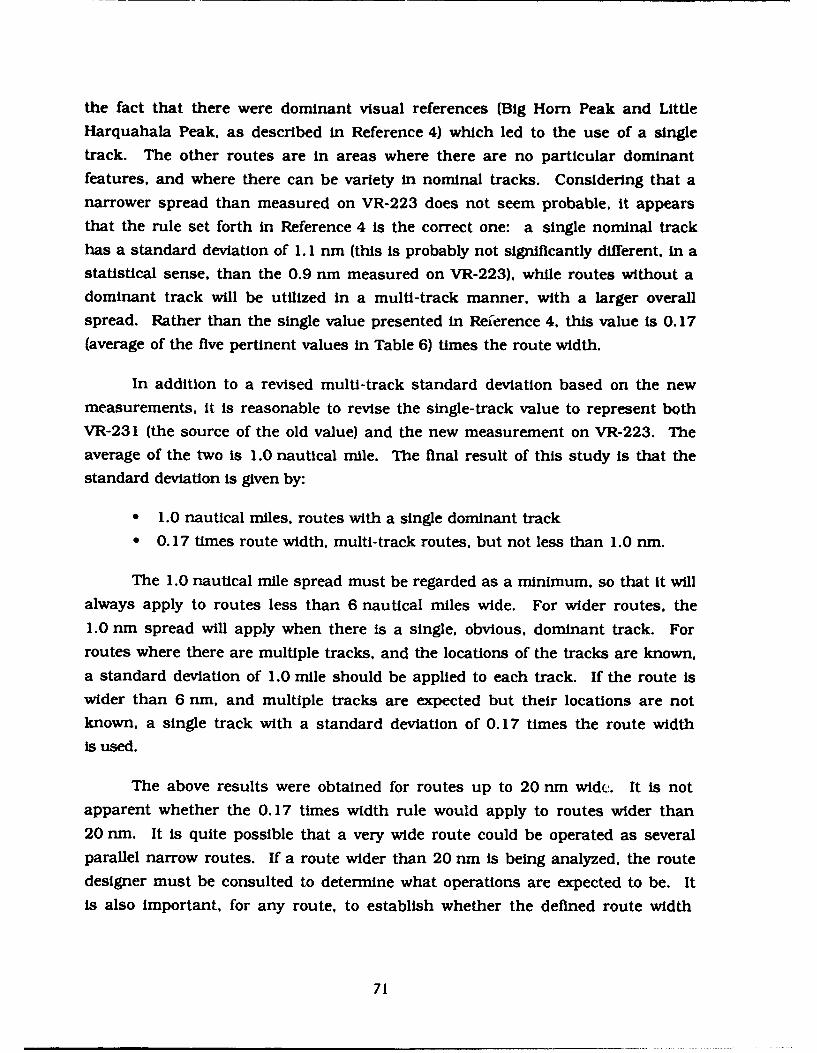
the fact that there were dominant visual references (Big Horn Peak and LittleHarquahala Peak, as described in Reference 4) which led to the use of a singletrack. The other routes are in areas where there are no particular dominant
features, and where there can be variety in nominal tracks. Considering that anarrower spread than measured on VR-223 does not seem probable, it appearsthat the rule set forth in Reference 4 is the correct one: a single nominal trackhas a standard deviation of 1. 1 nm (this is probably not significantly different, in astatistical sense, than the 0.9 nm measured on VR-223), while routes without adominant track will be utilized in a multi-track manner, with a larger overallspread. Rather than the single value presented in Reference 4, this value is 0.17(average of the five pertinent values in Table 6) times the route width.
In addition to a revised multi-track standard deviation based on the newmeasurements, it is reasonable to revise the single-track value to represent bothVR-231 (the source of the old value) and the new measurement on VR-223. Theaverage of the two is 1.0 nautical mile. The final result of this study is that thestandard deviation is given by:
* 1.0 nautical miles. routes with a single dominant track* 0.17 times route width, multi-track routes, but not less than 1.0 nm.
The 1.0 nautical mile spread must be regarded as a minimum, so that it willalways apply to routes less than 6 nautical miles wide. For wider routes, the1.0 rim spread will apply when there is a single, obvious, dominant track. Forroutes where there are multiple tracks, and the locations of the tracks are known,a standard deviation of 1.0 mile should be applied to each track. If the route iswider than 6 nm, and multiple tracks are expected but their locations are notknown, a single track with a standard deviation of 0.17 times the route width
is used.
The above results were obtained for routes up to 20 nm wide. It is not
apparent whether the 0.17 times width rule would apply to routes wider than20 nim. It is quite possible that a very wide route could be operated as severalparallel narrow routes. If a route wider than 20 rim is being analyzed, the routedesigner must be consulted to determine what operations are expected to be. Itis also important, for any route, to establish whether the defined route width
71

represents the actual usable portion of the route. This was the case for all routes
studied here (except for the Tabletop Mountain choke at the VR-223 measure-
ment site), and MTR analysis must be based on the usable route width.
The previous recommendation 4 had been to use a single value of 2.2 nm for
nominal multi-track routes. It is seen in Figures 33, 35. and 37 (which represent
routes 10 to 16 nm wide) that this single value yields centerline noise levels
within I dB of those obtained if the actual standard deviation is used. In the
overall assessment of airspace actions which involve many routes, it is reasonable
to use a single standard deviation of 2.2 run for routes between 10 and 16 nm
wide. It is also reasonable to establish similar average values for other width
ranges. In general. variation of the standard deviation by 25 to 30 percent leads to
sound level differences of no more than about 1 dB. When analyzing the impact
associated with a single specific route, however, the actual standard deviation for
that width should be used.
72
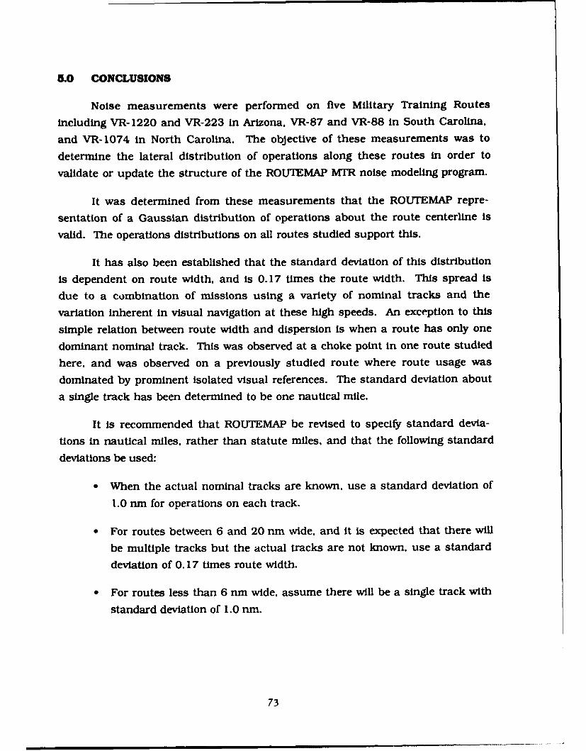
5.0 CONCLUSIONS
Noise measurements were performed on five Military Training Routes
including VR- 1220 and VR-223 in Arizona. VR-87 and VR-88 in South Carolina.
and VR-1074 in North Carolina. The objective of these measurements was to
determine the lateral distribution of operations along these routes in order to
validate or update the structure of the ROUTEMAP MTR noise modeling program.
It was determined from these measurements that the ROUTEMAP repre-
sentation of a Gaussian distribution of operations about the route centerline is
valid. The operations distributions on all routes studied support this.
It has also been established that the standard deviation of this distribution
is dependent on route width, and is 0.17 times the route width. This spread is
due to a combination of missions using a variety of nominal tracks and the
variation inherent in visual navigation at these high speeds. An exception to this
simple relation between route width and dispersion is when a route has only one
dominant nominal track. This was observed at a choke point in one route studied
here, and was observed on a previously studied route where route usage was
dominated by prominent isolated visual references. The standard deviation about
a single track has been determined to be one nautical mile.
It is recommended that ROUTEMAP be revised to specify standard devia-
tions in nautical miles, rather than statute miles, and that the following standard
deviations be used:
"* When the actual nominal tracks are known, use a standard deviation of
1.0 run for operations on each track.
"• For routes between 6 and 20 nm wide, and it is expected that there will
be multiple tracks but the actual tracks are not known, use a standard
deviation of 0.17 times route width.
"* For routes less than 6 nm wide, assume there will be a single track with
standard deviation of 1.0 nm.
73

* For routes wider than 20 nm. it is necessary to establish how the route
is used, then model it as either one wide route (extrapolating the
0. 17-times-width rule) or as a set of narrower routes.
When many routes are being analyzed for overMll assessment of a proposed
action, it is reasonable to use approximate values of the standard deviation, so long
as these are within 25 to 30 percent of the value from the above rules. If a single
route is being analyzed. the above rules should be followed.
74
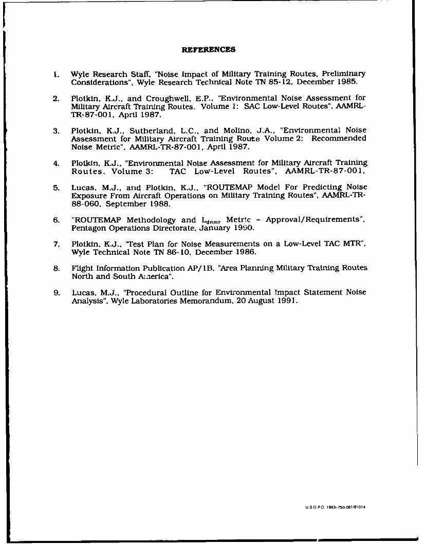
REFERENCES
1. Wyle Research Staff, "Noise Impact of Military Training Routes. PreliminaryConsiderations", Wyle Research Technical Note TN 85-12. December 1985.
2. Plotkin. K.J.. and Croughwell, E.P.. "Environmental Noise Assessment forMilitary Aircraft Training Routes. Volume 1: SAC Low-Level Routes". AAMRL-TR-87-001, April 1987.
3. Plotkin, K.J., Sutherland, L.C., and Molino, J.A., "Environmental NoiseAssessment for Military Aircraft Training Route Volume 2: RecommendedNoise Metric". AAMRL-TR-87-001, April 1987.
4. Plotkin, K.J., "Environmental Noise Assessment for Military Aircraft TrainingRoutes. Volume 3: TAC Low-Level Routes". AAMRL-TR-87-001,
5. Lucas, M.J., and Plotkin, K.J., "ROUTEMAP Model For Predicting NoiseExposure From Aircraft Operations on Military Training Routes", AAMRL-TR-88-060, September 1988.
6. "ROUTEMAP Methodology and Ldmr Metr!c - Approval/Requirements",Pentagon Operations Directorate, January 1990.
7. Plotkin. K.J., "Test Plan for Noise Measurements on a Low-Level TAC MTR".Wyle Technical Note TN 86-10, December 1986.
8. Flight Information Publication AP/ IB, "Area Planning Military Training RoutesNorth and South America".
9. Lucas. M.J.. "Procedural Outline for Environmental Tmpact Statement NoiseAnalysis", Wyle Laboratories Memorandum, 20 August 199 1.
US G PO 1993-750-061/81014