adaptive algorithms

�1

ADAPTIVE ALGORITHMS (EE654)

MIDTERM

-SUBMITTED BY

SAIDURGA SUBRAMANIAN

RED ID:817604600

DATE:12/1/2014

�2

1. An I-Q down converter, which forms I-Q signal components from a real input signal is shown below. The I and Q components are not orthogonal due to gain and phase imbalance as well as DC insertion in the two signal paths. An LMS based adaptive algorithm can remove the DC terms and balance the I-Q components. The model of the imbalance and DC injection is also shown below along with a model of the adaptive processes that repairs the signal.

!

!

A. We form 10000 sample complex sinusoidal input representing a (1.0/12)-KHz signal sampled at 10 KHz to simulate the input terms I(n) and Q(n). We set the phase imbalance and gain imbalance terms to 0.1 and the DC terms to 0.05 and 0.1 respectively and Form the distorted observed I and Q components. We are Plotting the 2048 point spectrum of the distorted and non distorted signal components and the Lissajous pattern (I vrs Q) for the non-distorted and for the distorted components. Pair of DC cancellers are implemented and the trajectory of the DC estimates are plotted for µ=0.01 and for µ =0.001 .Also , phase balancers and gain balancers are implemented

Low Pass

Low Pass

cos( t )ω0

s i n ( t + )ω α0- ( )1+ε

I’(t) I’(n)

Q’(t) Q’(n)

ADC

ADC

I I’

Q Q’

α1+ ε

DC I

DC Q

II’

QQ’

α

1- ε

- ^

^

^

^ αestimate

εestimate

DCCancel

DCCancel

�3

clc; clear all;

t=[0:9999];j=sqrt(-1); E=0.1; %gain dist a=0.1; %phase dist DC1=0.05;DC2=0.1; S=cos(2*pi*t*1/12)+j*(sin(2*pi*t*1/12)); I=cos(2*pi*t*1/12); Q=(sin(2*pi*t*1/12)); I1 =cos(2*pi*t*1/12)+DC1; Q1=((1+E)*(sin((2*pi*t*1/12)+a)))+DC2;

%A. figure(1) subplot(2,1,1) plot((-0.5:1/2048:0.5-1/2048)*12,fftshift(20*log10(abs(fft(I,2048))))) grid on title('Non distorted I component'); subplot(2,1,2) plot((-0.5:1/2048:0.5-1/2048)*12,fftshift(20*log10(abs(fft(Q,2048))))) grid on title('Non distorted Q component'); figure(2) subplot(2,1,1) plot((-0.5:1/2048:0.5-1/2048)*12,fftshift(20*log10(abs(fft(I1,2048))))) grid on title('Distorted I component'); subplot(2,1,2) plot((-0.5:1/2048:0.5-1/2048)*12,fftshift(20*log10(abs(fft(Q1,2048))))) grid on title('Distorted I component'); figure(3) subplot(1,2,1) plot(I,Q); axis('square') grid on title('Lissajous pattern- Non distorted') subplot(1,2,2) plot(I1,Q1); axis('square') grid on title('Lissajous pattern- Non distorted')

�4

figure(18) subplot(1,2,1) plot(I+j*Q,'.','linewidth',2) axis('square') title('Non Distorted I-Q') grid on subplot(1,2,2) plot(I1+j*Q1,'.','linewidth',2) axis('square') title('Distorted I-Q') grid on

%A.2. DC CANCELLER mu=0.01; reg=0;mu=0.01;dci1=0; for n=1:10000; y1=I1(n)-reg; %DC balanced I component i1_sv(n)=y1; reg=reg+mu*y1; dci1_sv(n,:)=reg; %DC estimate for I end

figure(4) plot(dci1_sv) grid on title('Dc trajectory of I component for mu=0.01') reg=0;mu=0.01;dcq1=0; for n=1:10000; y1=Q1(n)-reg; %DC balanced Q component q1_sv(n)=y1; reg=reg+mu*y1; dcq1_sv(n,:)=(reg); %DC estimate for Q end figure(5) plot(dcq1_sv) grid on title('Dc trajectory of Q component for mu=0.01') figure(6) subplot(1,2,1) plot(i1_sv,q1_sv); axis('square') grid on title('Lissajous pattern of I-Q component of DC canceller ,mu=0.01');

�5

subplot(1,2,2) plot(i1_sv+j*q1_sv,'.','linewidth',2) axis('square') title('DC cancelled I-Q'); grid on

%A.2.DC CANCELLER mu=0.001; reg=0;mu=0.001;dci2=0; for n=1:10000; y1=I1(n)-reg; i2_sv(n)=y1; %DC balanced I component reg=reg+mu*y1; dci2_sv(n,:)=reg; %DC estimate for I end figure(7) plot(dci2_sv) grid on

title('Dc trajectory of I component for mu=0.001') reg=0;mu=0.001;dcq2=0; for n=1:10000; y1=Q1(n)-reg; q2_sv(n)=y1; %DC balanced Q component reg=reg+mu*y1; dcq2_sv(n,:)=reg; %DC estimate for Q end figure(8) plot(dcq2_sv) grid on title('Dc trajectory of Q component for mu=0.001') figure(9) subplot(1,2,1) plot(i2_sv,q2_sv); axis('square') grid on title('Lissajous pattern of I-Q component of DC canceller ,mu=0.001'); subplot(1,2,2) plot(i2_sv+j*q2_sv,'.','linewidth',2) axis('square') title('DC cancelled I-Q'); grid on

�6

%B. PHASE BALANCER mu=0.01

reg=0;mu=0.01; for n=1:10000; y1=i1_sv(n); y=q1_sv(n)-(y1*reg); reg=reg+mu*y1*conj(y); qp1_sv(n)=y; %phase balanced q component aest_sv(n,:)=reg; %phase estimate end figure(10) plot(aest_sv) grid on hold off title('Phase estimate for mu=0.01') figure(11) subplot(1,2,1) plot(i1_sv,qp1_sv); axis('square') grid on title('Lissajous pattern of I-Q of phase balanced process ,mu=0.01'); subplot(1,2,2) plot(i1_sv+j*qp1_sv,'.','linewidth',2) axis('square') title('DC cancelled and phase balanced I-Q') grid on

%B. PHASE BALANCER mu=0.001

reg=0;mu=0.001; for n=1:10000; y1=i2_sv(n); y=q2_sv(n)-(y1*reg); reg=reg+mu*y1*conj(y); qp2_sv(n)=y; %phase balanced Q component aest_sv(n,:)=reg; %phase estimate end figure(12) plot(aest_sv) grid on title('Phase estimate for mu=0.001')

�7

figure(13) subplot(1,2,1) plot(i2_sv,qp2_sv); axis('square') grid on title('Lissajous pattern of I-Q of phase balanced process ,mu=0.001'); subplot(1,2,2) plot(i2_sv+j*qp2_sv,'.','linewidth',2) axis('square') title('DC cancelled and phase balanced I-Q') grid on

%C. Gain Balancer ; mu=0.01

reg=0;mu=0.01 for n=1:10000; y1=i1_sv(n); y=qp1_sv(n)-(reg); reg=reg+mu*y1*conj(y); qg1_sv(n)=y; %Gain Balanced Q component Eest_sv(n,:)=reg; %Gain estimate end figure(14) plot(Eest_sv) grid on title('Gain estimate for mu=0.01') figure(15) subplot(1,2,1) plot(i1_sv,qg1_sv); axis('square') grid on title('Lissajous pattern of I-Q of Gain balanced process ,mu=0.01'); subplot(1,2,2) plot(i1_sv+j*qg1_sv,'.','linewidth',2) axis('square') title('DC cancelled, phase and gain balanced I-Q') grid on

�8

%C. Gain Balancer ; mu=0.001

reg=0;mu=0.001;Eest=0; for n=1:10000; y1=i2_sv(n); y=qp2_sv(n)-(reg); reg=reg+mu*y1*conj(y); qg2_sv(n)=y; %Gain Balanced Q component Eest_sv(n,:)=reg; %Gain estimate end figure(16) plot(Eest_sv) grid on

title('Gain estimate for mu=0.001') figure(17) subplot(1,2,1) plot(i2_sv,qg2_sv); grid on title('Lissajous pattern of I-Q of Gain balanced process ,mu=0.001'); axis('square') subplot(1,2,2) plot(i2_sv+j*qg2_sv,'.','linewidth',2) title('DC cancelled and phase balanced I-Q') grid on axis('square')

�16

D. Simulate a 1,000,000 symbol QPSK signal set formed by random antipodal (± 1) I and Q components and have the cancellers with mu =0.00001 correct the imbalance defects with this signal. Plot the signal constellation at each point in the processing chain.

clear all; clc; close all ; x0=((floor(2*rand(1,1000000))-0.5)/0.5)+j*((floor(2*rand(1,1000000))-0.5)/0.5); I1=real(x0)+0.05; Q1=imag(x0)+0.1; %A.2. DC CANCELLER mu=0.00001; reg=0;mu=0.00001;dci1=0; for n=1:1000000; y1=I1(n)-reg; i1_sv(n)=y1; reg=reg+mu*y1; reg_sv(n)=reg; end figure(4) plot(reg_sv) grid on title('Dc trajectory of I component for mu=0.00001') grid on reg=0;mu=0.00001; reg_sv=zeros(1,1000000);

for n=1:1000000; y1=Q1(n)-reg; q1_sv(n)=y1; reg=reg+mu*y1; reg_sv(n)=reg; end figure(5) plot(reg_sv) grid on title('Dc trajectory of Q component for mu=0.00001') x3=i1_sv+j*q1_sv; figure(2) plot(0,0) plot(x3,'r.'); grid on axis('equal')

�18

2. A communication channel is formed by a cascade of four processes as shown below. The matched filter operates with the shaping filter to simultaneously maximize signal to noise ratio (SNR) and minimize inter symbol interference (ISI). The channel induced distortion introduces ISI and the equalizer serves to minimize its effect.

!

The input is 2000 samples of a complex QPSK random data sequence. The conventional shaping filter is a square root Nyquist filter with excess bandwidth α = 0.3 operating at 4-samples per symbol with 10-symbol delay to its peak response. We are going to replace the conventional shaping with a 9-Pole Inverse Chebyshev filter formed in MATLAB by cheby2(9,60,0.33025). This filter has the same 3-dB bandwidth and the same transition bandwidth as the SQRT Nyquist filter. The problem is it does not have linear phase. We want to see how the equalizer handles this problem. The channel impulse response is {1 0 0 0 0 0.2 0 0 j*0.1}, and the noise is complex AWGN with σ2=0.2. The receiver matched filter will be the conventional SQRT Nyquist filter.

Adaptive Control

r(t)s(t) x(t) y(t)Noise

Shaping Filter

Matched FilterChannel Equalizer

d(n)

�19

hh=rcosine(1,4,'sqrt',0.3,10); hh=hh/max(hh); [b,a]=cheby2(9,60,0.33025); h=filter(b,a,[1 zeros(1,100)]); h=h/max(h);

%a impulse and frequency response figure(1) subplot(2,2,1) plot(real(hh)); grid on title('Impulse response of Sqrt Nyquist Filter') subplot(2,2,2) plot(h(1:100)); grid on title('Impulse response of Cheby-2 Filter') subplot(2,2,3) plot((-0.5:1/2000:0.5-1/2000),fftshift(20*log10(abs(fft(hh/3.7,2000))))) grid on title('Frequency response of Sqrt Nyquist Filter') subplot(2,2,4) plot((-0.5:1/2000:0.5-1/2000),fftshift(20*log10(abs(fft(h/4.3,2000))))) grid on title('Frequency response of Cheby2 Filter')

%b pole zero diagram figure(2) subplot(2,1,1) zplane(hh); title('Pole-Zero Diagram of Sqrt Nyquist Filter') [z,p,k]=cheby2(9,60,0.33025); subplot(2,1,2) zplane(z,p); title('Pole-Zero Diagram of Cheby2 Filter')

%c shaping filter

x0=(floor(2*rand(1,2000))-0.5)/0.5+1i*((floor(2*rand(1,2000))-0.5)/0.5); x1=reshape([x0;zeros(3,2000)],1,8000); h=filter(b,a,[1 zeros(1,100)]); h=h/max(h); x2=filter(h,1,x1);

figure(3) subplot(3,1,1) plot(0:1/2:200,real(x2(1:401))); title('Time response by Shaping Filter')

subplot(2,2,3) plot(0,0) for n=3:8:8000-8

�20

hold on plot(-1:1/4:1,x2(n:n+8)); hold off end grid on axis('square') title('Eye diagram by Shaping Filter') subplot(2,2,4) plot(x2(3:4:8000),'r.'); grid on axis('equal') title(' Constellation Diagram by Shaping Filter')

%d channel output

chan=[1 0 0 0 0 0.2 0 0 j*0.1]; x3=filter(chan,1,x2) figure(4) subplot(3,1,1) plot(0:1/2:200,real(x3(1:401))); grid on title('Time response at Channel Output') subplot(2,2,3) plot(0,0) for n=3:8:8000-8 hold on plot(-1:1/4:1,x3(n:n+8)); hold off end grid on axis('square') title('Eye Diagram at Channel output') subplot(2,2,4) plot(x3(3:4:8000),'r.'); grid on axis('equal'); title('Constellation Diagram at Channel output')

%e matched filter output

x4=filter(hh,1,x3)/(hh*hh'); figure(5) subplot(3,1,1) plot(0:1/2:200,real(x4(1:401))); grid on title(' Time respnose at Matched Filter output') subplot(2,2,3) plot(0,0) for n=3:8:8000-8 hold on plot(-1:1/4:1,x4(n:n+8)); hold off end

�21

grid on axis('square') title('Eye Diagram at Matched filter output') subplot(2,2,4) plot(x4(3:4:4000),'r.'); axis('equal'); grid on title('Constellation Diagram at Matched filter output')

%f Equaliser output

m=1 offset=0; % center -position 33 %offset=24; %position 33+24 %offset=-24; %position 33-24 wts=[zeros(1,32+offset) 1 zeros(1,32-offset)]; reg2=zeros(1,65) mu=0.005; err_sv=0;er_sv=0;er1_sv=0; for n=3:4:8000-16 for k=1:4 reg2=[x4(n+k-1) reg2(1:64)]; x5(n+k-1)=reg2*wts'; if rem(n+k-1,4)==3 x6=sign(real(x5(n+k-1)))+j*sign(imag(x5(n+k-1))); err=x6-x5(n+k-1); err_sv(m)=err; wts=wts+mu*reg2*conj(err); m=m+1; er_sv(m)=(err)*(err); er1_sv(m)=abs(err)*abs(err); end end end figure(6)

subplot(2,2,3) plot(0,0) disp(x5) for n=403:8:8000-100 hold on plot(-1:1/4:1,x5(n:n+8)); hold off end grid on axis('square') title('Eye diagram at Equalizer output') subplot(2,2,4) plot(x5(403:4:8000-20),'r.'); grid on axis('equal') title(' Constellation Diagram at Equalizer output') subplot(3,1,1)

�22

plot(0:1/2:200,real(x5(1:401))); grid on title(' Time response at Equalizer output')

figure(7) hold on subplot(2,1,1) plot(abs(er_sv)); grid on title('Learning curve') hold off subplot(2,1,2) plot(20*log10(er1_sv)); grid on

�28

3.The IIR shaping filter is replaced with the SQRT Nyquist shaping filter and otherwise, except for the equalizer, apply the same operating conditions as in previous problem.

a. A 41 tap decision directed LMS equalizer, for this channel without the noise is operated . A short test is conducted to see where the initial unity valued weight should be located for best performance: (1 and 21).

b. A 41 tap FIR filter Goddard blind equalizer algorithm is used to equalize the channel (for p = 1, Sato Algorithm).

!

c. A 41 tap FIR filter Goddard blind equalizer algorithm is used to equalize the channel (for p = 2, CM Algorithm).

!

*

12

1

( 1) ( ) ( ) ( )( ) sgn[ ( )]( | ( ) |)

{| ( ) | }{| ( ) |}

µ+ = +

= −

=

W n W n x n e ne n y n R y n

E x nR

E x n

*

22

4

2 2

( 1) ( ) ( ) ( )( ) ( ) ( | ( ) | )

{| ( ) | }{| ( ) | }

W n W n x n e n

e n y n R y n

E x nR

E x n

µ+ = +

= −

=

�29

clear all; close all; clc; hh=rcosine(1,4,'sqrt',0.3,10); hh=hh/max(hh); %a

% shaping filter

x0=(floor(2*rand(1,2000))-0.5)/0.5+1i*((floor(2*rand(1,2000))-0.5)/0.5); h2=reshape(hh(1:80),4,20) reg=zeros(1,20) m=0; for n=1:2000 reg=[x0(n) reg(1:19)]; for k=1:4 x2(m+k)=reg*h2(k,:)'; end m=m+4; end

% channel output

chan=[1 0 0 0 0 0.2 0 0 j*0.1]; x3=filter(chan,1,x2) % matched filter -input to equaliser

x4=filter(hh,1,x3)/(hh*hh'); figure(1) subplot(3,1,1) plot(0:1/2:200,real(x4(1:401))); title('Time response of Equaliser input') grid on subplot(2,2,3) plot(0,0) for n=1:8:8000-8 hold on plot(-1:1/4:1,x4(n:n+8)); hold off end axis('square') grid on

�30

title('Eye Diagram of Equaliser input') subplot(2,2,4) plot(x4(1:4:4000),'r.'); axis('equal'); grid on title('Constellation Diagram of Equaliser input')

% Equaliser output

m=1 %wts=[1 zeros(1,40)] %1 at 1 wts=[zeros(1,20) 1 zeros(1,20)]; %1 at 21 reg2=zeros(1,41) mu=0.005; for n=1:4:8000 for k=1:4 reg2=[x4(n+k-1) reg2(1:40)]; x5(n+k-1)=reg2*wts'; if k==1 x6=sign(real(x5(n+k-1)))+j*sign(imag(x5(n+k-1))); err=x6-x5(n+k-1); err_sv(m)=err; wts=wts+mu*reg2*conj(err); m=m+1; er_sv(m)=(err)*(err); er1_sv(m)=abs(err)*abs(err); end end end figure(2) subplot(3,1,1) plot(0:1/2:200,real(x5(1:401))); title('Time response of Equaliser output') subplot(2,2,3) plot(0,0) for n=401:8:8000-8 hold on plot(-1:1/4:1,x5(n:n+8)); hold off end grid on

�31

axis('square') title('Eye Diagram of Equaliser output') subplot(2,2,4) plot(x5(401:4:8000),'r.'); grid on axis('equal') title('Constellation Diagram of Equaliser Output')

figure(3) hold on subplot(2,1,1) plot(abs(er_sv)); grid on title('Learning curve') hold off subplot(2,1,2) plot(20*log10(er1_sv)); grid on title('Learning curve with error power in dB')

%b Goddard blind equalizer algorithm to equalize the channel %( p = 1, Sato Algorithm)

m=1 %wts=[1 zeros(1,40)] %1 at 1 wts=[zeros(1,20) 1 zeros(1,20)]; %1 at 21 reg2=zeros(1,41) mu=0.005; err_sv=0;er1_sv=0; for n=1:4:8000 for k=1:4 reg2=[x4(n+k-1) reg2(1:40)]; x5(n+k-1)=reg2*wts'; if k==1 x6=sign(real(x5(n+k-1)))+j*sign(imag(x5(n+k-1))); R1=(abs(reg2).^2)/ (abs(reg2)) ; err=x6*(R1-(abs(x5(n+k-1)))); wts=wts+mu*reg2*conj(err); m=m+1; err_sv(m)=err;

�32

er_sv(m)=(err)*(err); er1_sv(m)=abs(err)*abs(err); end end end figure(4) subplot(3,1,1) plot(0:1/2:200,real(x5(1:401))); title('Time response of Equaliser Output') subplot(2,2,3) plot(0,0) for n=401:8:8000-8 hold on plot(-1:1/4:1,x5(n:n+8)); hold off end grid on axis('square') title('Eye Diagram of Equaliser Output') subplot(2,2,4) plot(x5(401:4:8000),'r.'); grid on axis('equal') title('Constellation Diagram of Equaliser Output')


�33

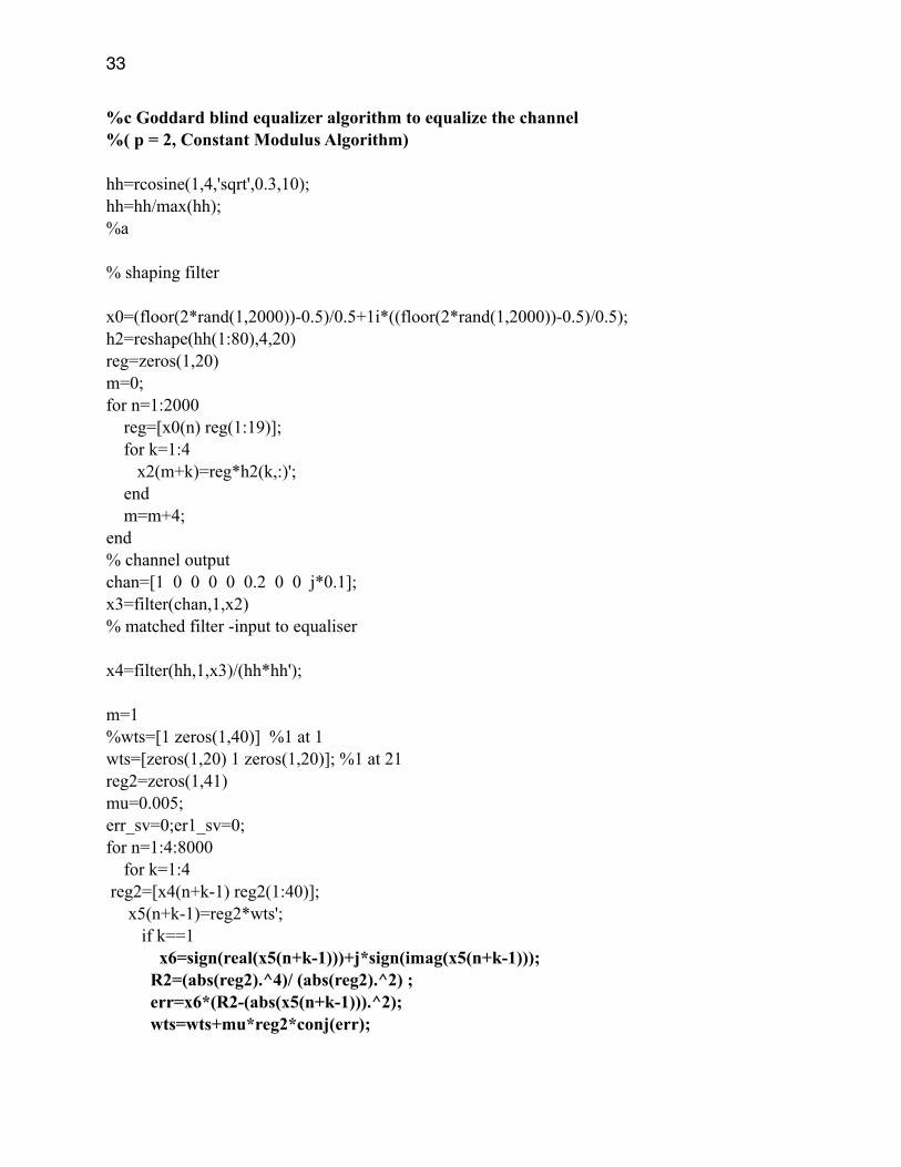
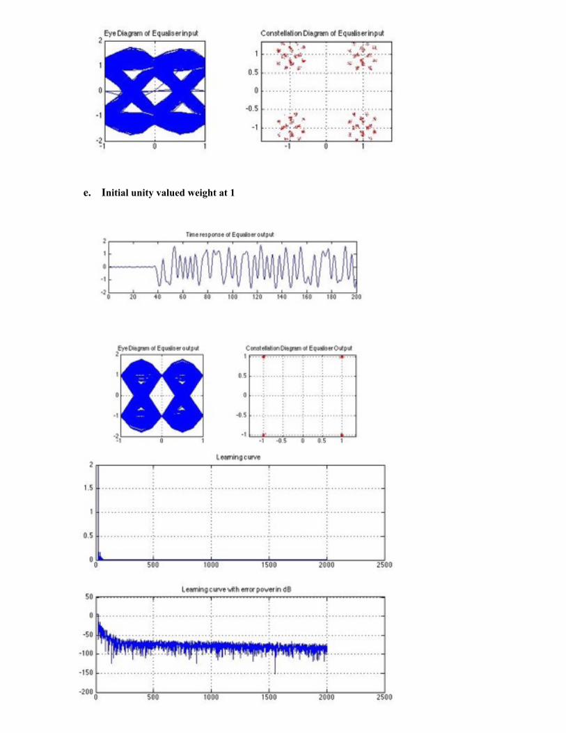
%c Goddard blind equalizer algorithm to equalize the channel %( p = 2, Constant Modulus Algorithm)

hh=rcosine(1,4,'sqrt',0.3,10); hh=hh/max(hh); %a

% shaping filter

x0=(floor(2*rand(1,2000))-0.5)/0.5+1i*((floor(2*rand(1,2000))-0.5)/0.5); h2=reshape(hh(1:80),4,20) reg=zeros(1,20) m=0; for n=1:2000 reg=[x0(n) reg(1:19)]; for k=1:4 x2(m+k)=reg*h2(k,:)'; end m=m+4; end % channel output chan=[1 0 0 0 0 0.2 0 0 j*0.1]; x3=filter(chan,1,x2) % matched filter -input to equaliser

x4=filter(hh,1,x3)/(hh*hh');

m=1 %wts=[1 zeros(1,40)] %1 at 1 wts=[zeros(1,20) 1 zeros(1,20)]; %1 at 21 reg2=zeros(1,41) mu=0.005; err_sv=0;er1_sv=0; for n=1:4:8000 for k=1:4 reg2=[x4(n+k-1) reg2(1:40)]; x5(n+k-1)=reg2*wts'; if k==1 x6=sign(real(x5(n+k-1)))+j*sign(imag(x5(n+k-1))); R2=(abs(reg2).^4)/ (abs(reg2).^2) ; err=x6*(R2-(abs(x5(n+k-1))).^2); wts=wts+mu*reg2*conj(err);

�34

m=m+1; err_sv(m)=err; er_sv(m)=(err)*(err); er1_sv(m)=abs(err)*abs(err); end end end figure(6) subplot(3,1,1) plot(0:1/2:200,real(x5(1:401))); title('Time response of Equaliser Output') subplot(2,2,3) plot(0,0) for n=401:8:8000-8 hold on plot(-1:1/4:1,x5(n:n+8)); hold off end grid on axis('square') title('Eye Diagram of Equaliser Output') subplot(2,2,4) plot(x5(401:4:8000),'r.'); grid on axis('equal') title('Constellation Diagram of Equaliser Output')


d.

�35

e. Initial unity valued weight at 1

�36

f. Initial unity valued weight at 21

�37

g. %b Goddard blind equalizer (Sato algorithm) Initial unity weight at 1

�38

%b Goddard blind equalizer (Sato algorithm) Initial unity weight at 21

�39

%c Goddard blind equalizer (Constant modulus algorithm) Initial unity weight at 1

�40

%c Goddard blind equalizer (Constant Modulus algorithm) Initial unity weight at 21

adaptive algorithms

Documents