albert a. montillo, ph.d. - temple universityhbling/8590.002/montillo_random...upenn & rutgers...

Albert A. Montillo, Ph.D.University of Pennsylvania, RadiologyRutgers University, Computer Science

Guest lecture: Statistical Foundations of Data AnalysisTemple University

4-2-2009

Random Forests

UPenn & Rutgers 2 of 28Albert A. Montillo

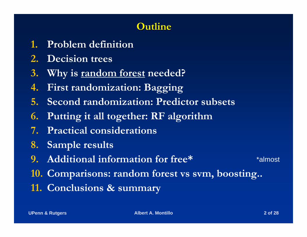
OutlineOutline

1. Problem definition 2. Decision trees 3. Why is random forest needed?4. First randomization: Bagging5. Second randomization: Predictor subsets6. Putting it all together: RF algorithm7. Practical considerations8. Sample results9. Additional information for free*10. Comparisons: random forest vs svm, boosting..11. Conclusions & summary

*almost


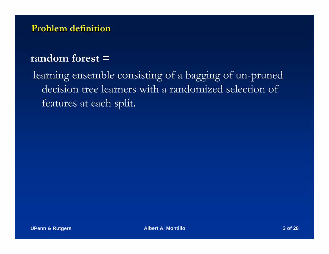
Problem definition Problem definition

random forest =

learning ensemble consisting of a bagging of un-pruned decision tree learners with a randomized selection of features at each split.


Decision treesDecision trees are the individual learners that are combinedare the individual learners that are combined

Decision trees … one of most popular learning methods commonly used for data exploration

One type of decision tree is called CART…classification and regression tree (Breiman 1983)

CART … greedy, top-down binary, recursive partitioning that divides feature space into sets of disjoint rectangular regions.

Regions should be pure wrt response variable.Simple model is fit in each region – majority vote for classification, constant value for regression


Decision treesDecision trees involve greedy, recursive partitioninginvolve greedy, recursive partitioning

Simple dataset with two predictors:

Greedy, recursive partitioning along TI and PE:


Model of underlying functional form sought from datageneral decision trees

Score criterion to judge quality of fit of model

Search strategy to minimize the score criterion

Decision trees:Decision trees: model, score criterion, search strategymodel, score criterion, search strategy

{ }1 2 1: , , ,..., { , }

# #

Ni i ii i ikTraining set D y x x x y

where k predictors and N samples= =

= =

x


Decision trees:Decision trees: AlgorithmAlgorithm

Grow tree until minimum node size (e.g. 5) is reached. Then prune tree using cost-complexity pruning.


Larger the tree, more likely of overfitting training data.

Pruning finds subtree that generalizes beyond training data

Essence is to trading off tree complexity (size) and goodness of fit to the data (node purity).

Efficient split yields pure children: Rl and Rr

Decision trees:Decision trees: avoid avoid overfittingoverfitting through pruningthrough pruning


Regression –simple case; use squared error impurity measure. Let Rm = Rl and Nm denote # samples falling into Rm. Impurity of Rm for subtree T is given by Qm(T):

Classification – squared error not suitable. Instead use: misclassification error, Gini index, or deviance. [see ESL ch 9]

Pruning involves finding the subtree T that minimizes the cost complexity objective function:

For details see [Breiman 1984]

Decision trees:Decision trees: Efficiency of split measured through node purityEfficiency of split measured through node purity


Why RF?Why RF? Decision trees: Decision trees: Advantages and Advantages and limitations limitations

Advantages:

Limitations:Low prediction accuracyHigh variance

Ensemble, to maintain advantages while increasing accuracy !


Random forest: first randomization through Random forest: first randomization through baggingbagging

Bagging = bootstrap aggregation (Breiman 1996)

Bootstrap sample = create new training sets by random sampling the given one N′≤N times with replacement

Bootstrap aggregation … parallel combination of learners, independently trained on distinct bootstrap samples

Final prediction is the mean prediction (regression) or class with maximum votes (classification).

Using squared error loss, bagging alone decreases test error by lowering prediction variance, while leaving bias unchanged.


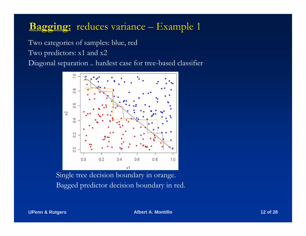
Bagging:Bagging: reduces variance reduces variance –– Example 1Example 1Two categories of samples: blue, redTwo predictors: x1 and x2Diagonal separation .. hardest case for tree-based classifier

Single tree decision boundary in orange. Bagged predictor decision boundary in red.


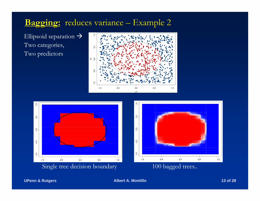
Bagging:Bagging: reduces variance reduces variance –– Example 2Example 2Ellipsoid separation Two categories, Two predictors

Single tree decision boundary 100 bagged trees..


Bagging alone utilizes the same full set of predictors to determine each split.

However random forest applies another judicious injection of randomness: namely by selecting a random subset of the predictors for each split (Breiman 2001)

Number of predictors to try at each split is known as mtry. While this becomes new parameter, typically (classification) or (regression) works quite well. RF is not overly sensitive to mtry

Bagging is a special case of random forest where mtry=k

Random forest: second randomization through Random forest: second randomization through predictor subsetspredictor subsets

trym k=

3try km =


Overall the additional randomness: further reduces variance even on smaller sample set sizes, improving accuracy

however significantly lowering predictor set at each node might lower accuracy, particularly if there are few good predictors among many non-informative “predictors”

Subset of predictors much faster to search than all predictors

Random forest: second randomization through Random forest: second randomization through predictor subsetspredictor subsets


Random forest algorithmRandom forest algorithm

Let Ntrees be the number of trees to buildfor each of Ntrees iterations

1. Select a new bootstrap sample from training set2. Grow an un-pruned tree on this bootstrap. 3. At each internal node, randomly select mtry predictors and

determine the best split using only these predictors.4. Do not perform cost complexity pruning. Save tree as is,

along side those built thus far.

Output overall prediction as the average response (regression) or majority vote (classification) from all individually trained trees


Random forest algorithmRandom forest algorithm (flow chart)(flow chart)

For computer scientists:


Random forest:Random forest: practical considerationspractical considerations

Splits are chosen according to a purity measure: e.g. squared error (regression), Gini index or deviance (classification) [see ESL ch 9]

How to select Ntrees? Build trees until the error no longer decreases

How to select mtry ? Try the recommended defaults, half of them and twice them and pick the best


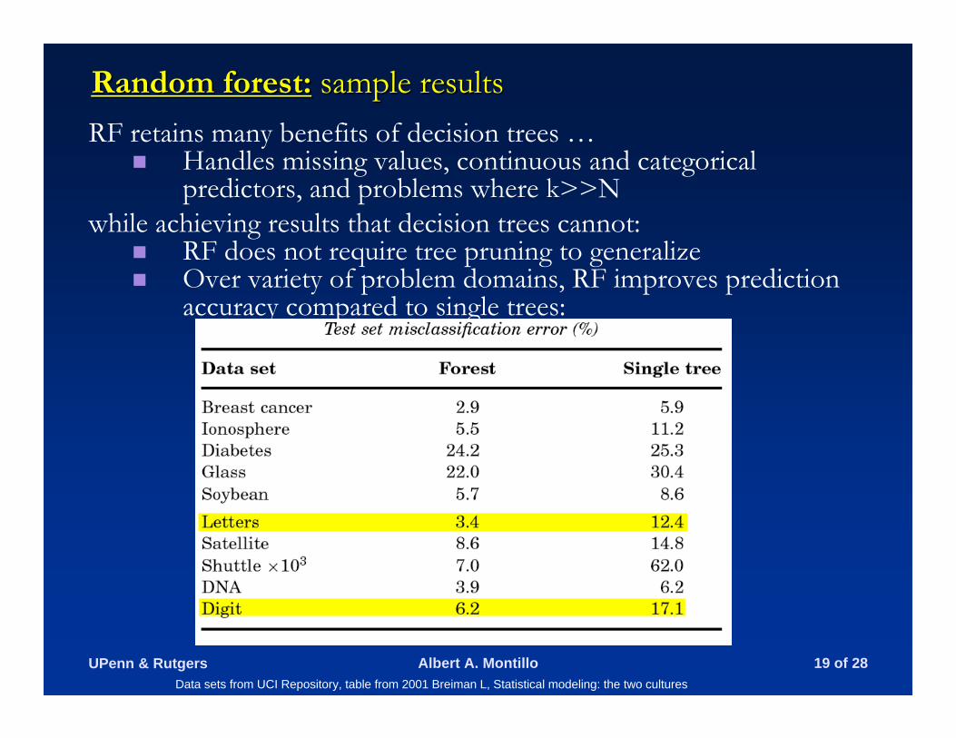
Random forest:Random forest: sample resultssample resultsRF retains many benefits of decision trees …

Handles missing values, continuous and categorical predictors, and problems where k>>N

while achieving results that decision trees cannot:RF does not require tree pruning to generalizeOver variety of problem domains, RF improves prediction accuracy compared to single trees:

Data sets from UCI Repository, table from 2001 Breiman L, Statistical modeling: the two cultures


Random forest:Random forest: Additional information for free* Estimating the test error:

While growing forest, estimate test error from training samples

For each tree grown, 33-36% of samples are not selected in bootstrap, called out of bootstrap (OOB) samples [Breiman 2001]

Using OOB samples as input to the corresponding tree, predictions are made as if they were novel test samples

Through book-keeping, majority vote (classification), average (regression) is computed for all OOB samples from all trees.

Such estimated test error is very accurate in practice, with reasonable Ntrees

*almost free


Random forest:Random forest: Additional information for free*

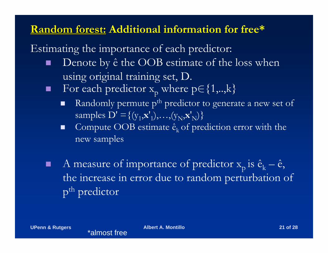
Estimating the importance of each predictor:Denote by ê the OOB estimate of the loss when using original training set, D.For each predictor xp where p∈{1,..,k}

Randomly permute pth predictor to generate a new set of samples D' ={(y1,x'1),…,(yN,x'N)}Compute OOB estimate êk of prediction error with the new samples

A measure of importance of predictor xp is êk – ê, the increase in error due to random perturbation of pth predictor

*almost free


Random forest:Random forest: Additional information for free*

Estimating the similarity of samples:During growth of the forest

Keep track of the number of times, samples xi and xjappear in the same terminal nodeNormalize by NtreesStore all normalized co-occurrences in a matrix, denoted as the proximity matrix.

Proximity matrix can be considered a kind of similarity measure between any two samples xi and xjCan even use a clustering method to perform unsupervised learning from RF. For details see [Liaw A, 2002]

*almost free


Comparisons:Comparisons: random forest random forest vsvs SVMsSVMs, neural networks, neural networksRandom forests have about same accuracy as SVMs and neural networks

RF is more interpretableFeature importance can be estimated during training for little additional computationPlotting of sample proximitiesVisualization of output decision trees

RF readily handles larger numbers of predictors.

Faster to train

Has fewer parameters

Cross validation is unnecessary : It generates an internal unbiased estimate of the generalization error (test error) as the forest building progresses


Comparisons:Comparisons: random forest random forest vsvs boostingboosting

Main similarities:Both derive many benefits from ensembling, with few disadvantagesBoth can be applied to ensembling decision trees.

Main differences:Boosting performs an exhaustive search for best predictor to split on; RF searches only a small subset

Boosting grows trees in series, with later trees dependent on the results of previous trees; RF grows trees in parallel independently of one another.


Comparisons:Comparisons: random forest random forest vsvs boostingboostingWhich one to use and when…

RF has about the same accuracy as boosting for classification, For continuous response, boosting appears to outperform RF

Boosting may be more difficult to model and requires more attention to parameter tuning than RF.

On very large training sets, boosting can become slow with many predictors, while RF which selects only a subset of predictors for each split, can handle significantly larger problems before slowing.

RF will not overfit the data. Boosting can overfit (though means can be implemented to lower the risk of it).

If parallel hardware is available, (e.g. multiple cores), RF embarrassingly parallel with out the need for shared memory as all trees are independent


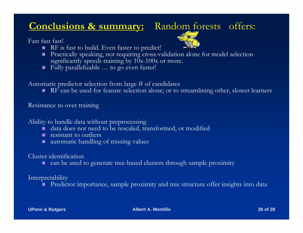
Conclusions & summary:Conclusions & summary: Random forests offers:Fast fast fast!

RF is fast to build. Even faster to predict!Practically speaking, not requiring cross-validation alone for model selection significantly speeds training by 10x-100x or more. Fully parallelizable … to go even faster!

Automatic predictor selection from large # of candidates RF can be used for feature selection alone; or to streamlining other, slower learners

Resistance to over training

Ability to handle data without preprocessing data does not need to be rescaled, transformed, or modified resistant to outliers automatic handling of missing values

Cluster identification can be used to generate tree-based clusters through sample proximity

Interpretability Predictor importance, sample proximity and tree structure offer insights into data


References:References:1984, Breiman L, Friedman J, Olshen R, Stone C, Classification and Regression Trees;

Chapman & Hall; New York

1996, Breiman L, Bagging Predictors. Machine Learning 26, pp 123-140.

2001, Breiman L, Random Forests. Machine Learning, 45 (1), pp 5-32.

2001, Breiman L, Statistical modeling: the two cultures, Statistical Science 2001, Vol. 16, No. 3, 199-231

2001, Hastie T, Tibshirani R, Freidman J, The Elements of Statistical Learning; Springer; New York

2002, Salford Systems; Salford Systems White Paper Series, www.salford-systems.com

2002, Liaw A, Wiener M, Classification and Regression by Random Forest, R News, Vol2/3, Dec

2002, Breiman L, Looking inside the black box, Wald Lecture Series II2005, Cutler, Random Forests, Encyclopedia of Statistics in Behavioral Science, pp 1665–

1667.2006, Sandri M, Zuccolotto P, Variable selection using random forests, Data analysis,

classificaiton and the forward search, Springer, pp. 263-270


Thank youThank you

… Questions?

albert a. montillo, ph.d. - temple universityhbling/8590.002/montillo_random...upenn & rutgers...

Documents