Algorithms for data streams

Camil Demetrescu ∗ Irene Finocchi †

July 26, 2006

Abstract

Data stream processing has gained increasing popularity in the last few years as

an effective paradigm for processing massive data sets. A wide range of applications

in computational sciences generate huge and rapidly changing data streams that need

to be continuously monitored in order to support exploratory analyses and to detect

correlations, rare events, fraud, intrusion, unusual or anomalous activities. Relevant

examples include monitoring network traffic, online auctions, transaction logs, tele-

phone call records, automated bank machine operations, atmospheric and astronomical

events. Due to the high sequential access rates of modern disks, streaming algorithms

can also be effectively deployed for processing massive files on secondary storage, pro-

viding new insights into the solution of several computational problems in external

memory.

Streaming models constrain algorithms to access the input data in one or few se-

quential passes, using only a small amount of working memory and processing each

input item quickly. Solving computational problems under these restrictions poses sev-

eral algorithmic challenges. This chapter is intended as an overview and survey of the

main models and techniques for processing data streams and their applications.

∗Dipartimento di Informatica e Sistemistica, Universita di Roma “La Sapienza”, Roma, Italy. Email:

demetres@dis.uniroma1.it. URL: http://www.dis.uniroma1.it/~demetres.†Dipartimento di Informatica, Universita di Roma “La Sapienza”, Roma, Italy. Email:

finocchi@di.uniroma1.it. URL: http://www.dsi.uniroma1.it/~finocchi.

Contents

1 Introduction 51.1 Applications . . . . . . . . . . . . . . . . . . . . . . . . . . . . . . . . . . . . 5

1.1.1 Network management . . . . . . . . . . . . . . . . . . . . . . . . . . . 61.1.2 Database monitoring . . . . . . . . . . . . . . . . . . . . . . . . . . . 61.1.3 Sequential disk accesses . . . . . . . . . . . . . . . . . . . . . . . . . 7

1.2 Overview to the literature . . . . . . . . . . . . . . . . . . . . . . . . . . . . 71.3 Chapter outline . . . . . . . . . . . . . . . . . . . . . . . . . . . . . . . . . . 8

2 Data stream models 92.1 Classical streaming . . . . . . . . . . . . . . . . . . . . . . . . . . . . . . . . 92.2 Semi-streaming . . . . . . . . . . . . . . . . . . . . . . . . . . . . . . . . . . 92.3 Streaming with a sorting primitive . . . . . . . . . . . . . . . . . . . . . . . 10

3 Algorithm design techniques 103.1 Sampling . . . . . . . . . . . . . . . . . . . . . . . . . . . . . . . . . . . . . . 11

3.1.1 Reservoir sampling . . . . . . . . . . . . . . . . . . . . . . . . . . . . 113.1.2 An application of sampling: frequent items . . . . . . . . . . . . . . . 12

3.2 Sketches . . . . . . . . . . . . . . . . . . . . . . . . . . . . . . . . . . . . . . 143.2.1 Probabilistic counting . . . . . . . . . . . . . . . . . . . . . . . . . . 153.2.2 Randomized linear projections . . . . . . . . . . . . . . . . . . . . . . 17

3.3 Techniques for graph problems . . . . . . . . . . . . . . . . . . . . . . . . . . 183.4 Simulation of PRAM algorithms . . . . . . . . . . . . . . . . . . . . . . . . . 20

4 Lower bounds 224.1 Randomization . . . . . . . . . . . . . . . . . . . . . . . . . . . . . . . . . . 234.2 Approximation . . . . . . . . . . . . . . . . . . . . . . . . . . . . . . . . . . 244.3 Randomization and approximation . . . . . . . . . . . . . . . . . . . . . . . 25

5 Conclusions 26

1 Introduction

Efficient processing over massive data sets has taken an increased importance in the lastyears due to the growing availability of large volumes of data in a variety of applicationsin computational sciences. In particular, monitoring huge and rapidly changing streams ofdata that arrive on-line has emerged as an important data management problem: relevantapplications include analyzing network traffic, online auctions, transaction logs, telephonecall records, automated bank machine operations, atmospheric and astronomical events. Forthese reasons, the streaming model has recently received a lot of attention []. This modeldiffers from computation over traditional stored datasets since algorithms must process theirinput by making one or a small number of passes over it, using only a limited amount ofworking memory. The streaming model applies to settings where the size of the input farexceeds the size of the main memory available and the only feasible access to the data is bymaking one or more passes over it.

Typical streaming algorithms use space at most poly-logarithmic in the length of theinput stream and must have fast update and query times. Using sublinear space motivatesthe design for summary data structures with small memory footprints, also known as syn-opses [31]. Queries are answered using information provided by these synopses, and it maybe therefore impossible to produce an exact answer. The challenge is thus to produce high-quality approximate answers, i.e., answers with confidence bounds on the possible error:accuracy guarantees are typically made in terms of a pair of user-specified parameters, ε andδ, meaning that the error in answering a query is within a factor of ε with probability atleast 1 − δ. The space and update time will consequently depend on these parameters andthe goal is to limit this dependence as much as possible.

Major progress has been achieved in the last ten years in the design of streaming al-gorithms for several fundamental data sketching and statistics problems, for which severaldifferent synopses have been proposed. Examples include number of distinct items, frequencymoments, L1 and L2 norms of vectors, inner products, frequent items, heavy hitters, quan-tiles, histograms, wavelets. Recently, progress has been achieved for other problem classes,including computational geometry (e.g., clustering and minimum spanning trees) and graphs(e.g., triangle counting and spanners). At the same time, there has been a flurry of activityin proving impossibility results, devising interesting lower bound techniques and establishingimportant complementary results.

This chapter is intended as an overview of this rapidly evolving area. The chapter is notmeant to be comprehensive, but rather aims at providing an outline of the main techniquesused for designing algorithms or for proving lower bounds. We refer the interested reader to[7, 31, 51] for an extensive discussion of problems and results not mentioned here.

1.1 Applications

As observed before, the primary application of data stream algorithms is to monitor contin-uously huge and rapidly changing streams of data in order to support exploratory analysesand to detect correlations, rare events, fraud, intrusion, unusual or anomalous activities.

5

Such streams of data may be, e.g., performance measurements in traffic management, all de-tail records in telecommunications, transactions in retail chains, ATM operations in banks,log records generated by Web Servers, or sensor network data. In all these cases, the vol-umes of data are huge (several Terabytes or even Petabytes), and records arrive at a rapidrate. Other relevant applications for data stream processing are related, e.g., to processingmassive files on secondary storage and to monitoring the contents of large databases or datawarehouse environments. In this section we highlight some typical needs that arise in thesecontexts.

1.1.1 Network management

Perhaps the most prominent application is related to network management, that involvesmonitoring and configuring network hardware and software to ensure smooth operations.Consider, e.g., traffic analysis in the Internet. Here, as information on IP packets flowsthrough the routers, we would like to monitor link bandwidth usage, to estimate trafficdemands, to detect faults, congestion, usage patterns. Typical queries that we would be ableto answer are thus the following. How many IP addresses used a given link in a certain periodof time? How many bytes were sent between a pair of IP addresses? Which are the top 100IP addresses in terms of traffic? What is the average duration of an IP session? Whichsessions transmitted more than 1000 bytes? Which IP addresses are involved in more than1000 sessions? All these queries are heavily motivated by traffic analysis, fraud detection,and security.

To get a rough estimate of the amount of data that need to be analyzed to answer onesuch query, consider that each router can forward up to 1 Billion packets per hour, and eachInternet Service Provider may have many hundreds of routers: thus, many Terabytes of dataneed to be processed. This data arrive at a rapid rate, and we therefore need algorithmsto mine patterns, process queries, and compute statistics on such data streams in almostreal-time.

1.1.2 Database monitoring

Many commercial database systems have a query optimizer used for estimating the cost ofcomplex queries. Consider, e.g., a large database that undergoes transactions (includingupdates). Upon the arrival of a complex query q, the optimizer may run some simple queriesin order to decide an optimal query plan for q: in particular, a principled choice of anexecution plan by the optimizer depends heavily on the availability of statistical summariessuch as histograms, the number of distinct values in a column for the tables referenced ina query, or the number of items that satisfy a given predicate. The optimizer uses thisinformation to decide between alternative query plans and to optimize the use of resourcesin multiprocessor environments. The accuracy of the statistical summaries greatly impactsthe ability to generate good plans for complex SQL queries. The summaries, however, mustbe computed quickly: in particular, examining the entire database is typically regarded asprohibitive.

6

1.1.3 Sequential disk accesses

In modern computing platforms, the access times to main memory and disk varies by severalorders of magnitude. Hence, when the data resides on disk, it is much more important tominimize the number of I/Os (i.e., the number of disk accesses) than the CPU computationtime as it is done in traditional algorithms theory. Many ad-hoc algorithmic techniques havebeen proposed in the external memory model for minimizing the number of I/Os during acomputation (see, e.g., [58]).

Due to the high sequential access rates of modern disks, streaming algorithms can alsobe effectively deployed for processing massive files on secondary storage, providing newinsights into the solution of several computational problems in external memory. In manyapplications managing massive data sets, using secondary and tertiary storage devices isindeed a practical and economical way to store and move data: such large and slow externalmemories, however, are best optimized for sequential access, and thus naturally produce hugestreams of data that need to be processed in a small number of sequential passes. Typicalexamples include data access to database systems [36] and analysis of Internet archives storedon tape [40]. The streaming algorithms designed with these applications in mind may havea greater flexibility: indeed, the rate at which data are processed can be adjusted, datacan be processed in chunks, and more powerful processing primitives (e.g., sorting) may beavailable.

1.2 Overview to the literature

The problem of computing in a small number of passes over the data appears already inpapers from the early 80’s. Munro and Paterson [50], for instance, studied the space requiredfor selection when at most P passes over the data can be performed, giving almost matchingupper and lower bounds as a function of P and of the input size. The paper by Alon,Matias and Szegedy [5, 6], awarded with the Godel Prize for outstanding papers in the areaof theoretical computer science in 2005, provided the foundations of the field of streamingand sketching algorithms. This seminal work introduced the novel technique of designingsmall randomized linear projections that allow it to approximate to user-specified precisionthe frequency moments of a data sets and other quantities of interest. The computation offrequency moments is now fully understood, with almost matching upper and lower bounds(up to polylogarithmic factors) [9, 11, 17, 43, 56].

Since 1996, many fundamental data statistics problems have been efficiently solved instreaming models. For instance, the computation of frequent items is particularly relevantin network monitoring applications, and has been addressed, e.g., in [1, 13, 19, 20, 46, 49].A plethora of other problems have been studied in the last years, designing solutions thathinge upon many different and interesting techniques. Among them, we recall sampling,probabilistic counting, combinatorial group testing, core-sets, dimensionality reduction, tree-based methods. We will provide examples of application of some of these techniques inSection 3. An extensive bibliography can be found in [51]. The development of advancedtechniques made it possible to solve progressively more complex problems, including the

7

computation of histograms, quantiles, norms, as well as geometric and graph problems.Histograms capture the distribution of values in a data set by grouping values into buckets

and maintaining suitable summary statistics for each bucket. Different kinds of histogramsexist: e.g., in an equi-depth histogram the number of values falling into each bucket is uniformacross all buckets. The problem of computing these histograms is strictly related to theproblem of maintaining the quantiles for the data set: quantiles represent indeed the bucketboundaries. These problems have been addressed, e.g., in [15, 33, 34, 37, 38, 50, 52, 53].Wavelets are also widely used to provide summarized representations of data: works oncomputing wavelet coefficients in data stream models include [4, 34, 35, 54].

A few fundamental works consider problems related to norm estimation, e.g., dominancenorms and Lp sums [18, 41]. In particular, Indyk pioneered the design of sketches based onrandom variables drawn from stable distributions (which are known to exist) and appliedthis idea to the problem of estimating Lp sums [41].

Geometric problems have been also the subject of much recent research in the streamingmodel [28, 29, 42]. In particular, clustering problems received special attention: given aset of points with a distance function defined on them, the goal is to find a clusteringsolution (a partition into clusters) that optimizes a certain objective function. Classicalobjective functions include minimizing the sum of distances of points to their closest median(k-median) or minimizing the maximum distance of a point to its closest center (k-center).Streaming algorithms for such problem are presented, e.g., in [14, 39].

Differently from most data statistics problems, where O(1) passes and polylogarithmicworking space have been proven to be enough to find approximate solutions, many classicalgraph problems seem to be far from being solved within similar bounds: for many classicalgraph problems linear lower bounds on the space × passes product are indeed known [40].A notable exception is related to counting triangles in graphs, as discussed in [10]. Somerecent papers show that several graph problems can be solved with one or few passes in thesemi-streaming model [23, 24, 25, 48] where the working memory size is O(n · polylog n) foran input graph with n vertices: in other words, akin to semi-external memory models [2, 58]there is enough space to store vertices, but not edges of the graph. Other works, suchas [3, 22, 55], consider the design of streaming algorithms for graph problems when themodel allows more powerful primitives for accessing stream data (e.g., use of intermediatetemporary streams and sorting).

1.3 Chapter outline

This chapter is organized as follows. In Section 2 we describe the most common data streammodels: such models differ in the interpretation of the data on the stream (each item caneither be a value itself or indicate an update to a value) and in the primitives available foraccessing and processing stream items. In Section 3 we focus on techniques for proving upperbounds: we describe some mathematical and algorithmic tools that have proven to be usefulin the construction of synopsis data structures (including randomization, sampling, hashing,probabilistic counting) and we first show how these techniques can be applied to classicaldata statistics problems. We then move to consider graph problems as well as techniques

8

useful in streaming models that provide more powerful primitives for accessing stream datain a non-local fashion (e.g., simulations of parallel algorithms). In Section 4 we address somelower bound techniques for streaming problems, using the computation of the number ofdistinct items in a data stream as a running example: we explore the use of reductions ofproblems in communication complexity to streaming problems, and we discuss the use ofrandomization and approximation in the design of efficient synopses. In Section 5 we sumup, suggesting directions for further research.

2 Data stream models

A variety of models exists for data stream processing: the differences depend on how streamdata should be interpreted and which primitives are available for accessing stream items. Inthis section we overview the main features of the most commonly used models.

2.1 Classical streaming

In classical data streaming [5, 40, 50, 51], input data is accessed sequentially in the formof a data stream Σ = x1, ..., xn, and need to be processed using a working memory thatis small compared to the length n of the stream. The main parameters of the model arethe number p of sequential passes over the data, the size s of the working memory, and theper-item processing time. All of them should be kept small: typically, one strives for 1 passand polylogarithmic space, but this is not a requirement of the model.

There exist at least three variants of classical streaming, dubbed (in increasing order ofgenerality) time series, cash register, and turnstile [51]. Indeed, we can think of stream itemsx1, ..., xn as describing an underlying signal A, i.e., a one dimensional function over the reals.In the time series model each stream item xi represents the i-th value of the underlyingsignal, i.e., xi = A[i]. In the other models each stream item xi represents an update of thesignal: namely, xi can be thought of as a pair (j, Ui), meaning that the j-th value of theunderlying signal must be changed by the quantity Ui, i.e. Ai[j] = Ai−1[j]+Ui. The partiallydynamic scenario in which the signal can be only incremented, i.e., Ui ≥ 0, corresponds tothe cash register model, while the fully dynamic case yields the turnstile model.

2.2 Semi-streaming

Despite the heavy restrictions of classical data streaming, we will see in Section 3 thatmajor success has been achieved for several data sketching and statistics problems, whereO(1) passes and polylogarithmic working space have been proven to be enough to findapproximate solutions. On the other hand, there exist many natural problems (includingmost problems on graphs) for which linear lower bounds on p × s are known, even usingrandomization and approximation: these problems cannot be thus solved within similarpolylogarithmic bounds. Some recent papers [24, 25, 48] have therefore relaxed the polylogspace requirements considering a semi-streaming model, where the working memory size is

9

O(n · polylog n) for an input graph with n vertices: in other words, akin to semi-externalmemory models [2, 58], there is enough space to store vertices, but not edges of the graph. Wewill see in Section 3.3 that some complex graph problems can be solved in semi-streaming,including spanners, matching, and diameter estimation.

2.3 Streaming with a sorting primitive

Motivated by technological factors, some authors have recently started to investigate thecomputational power of even less restrictive streaming models. Today’s computing platformsare equipped with large and inexpensive disks highly optimized for sequential read/writeaccess to data, and among the primitives that can efficiently access data in a non-localfashion, sorting is perhaps the most optimized and well understood. These considerationshave led to introduce the stream-sort model [3, 55]. This model extends classical streamingin two ways: the ability to write intermediate temporary streams and the ability to reorderthem at each pass for free. A stream-sort algorithm alternates streaming and sorting passes:a streaming pass, while reading data from the input stream and processing them in theworking memory, produces items that are sequentially appended to an output stream; asorting pass consists of reordering the input stream according to some (global) partial orderand producing the sorted stream as output. Streams are pipelined in such a way thatthe output stream produced during pass i is used as input stream at pass (i + 1). Wewill see in Section 3.4 that the combined use of intermediate temporary streams and of asorting primitive yields enough power to solve efficiently (within polylogarithmic passes andmemory) a variety of graph problems that cannot be solved in classical streaming. Evenwithout sorting, the model is powerful enough for achieving space-passes tradeoffs [22] forgraph problems for which no sublinear memory algorithm is known in classical streaming.

3 Algorithm design techniques

Since data streams are potentially unbounded in size, when the amount of computationmemory is bounded it may be impossible to produce an exact answer. In this case, the chal-lenge is to produce high-quality approximate answers, i.e., answers with confidence boundson the possible error. The typical approach is to maintain a “lossy” summary of the datastream by building up a synopsis data structure with memory footprint substantially smallerthan the length of the stream. In this section we describe some mathematical and algo-rithmic techniques that have proven to be useful in the construction of such synopsis datastructures. Besides the ones considered in this chapter, many other interesting techniqueshave been proposed: the interested reader can find pointers to relevant works in Section 1.2.

The most natural approach to designing streaming algorithms is perhaps to maintain asmall sample of the data stream: if the sample captures well the essential characteristics ofthe entire data set with respect to a specific problem, evaluating a query over the samplemay provide reliable approximation guarantees for that problem. In Section 3.1 we discusshow to maintain a bounded size sample of a (possibly unbounded) data stream, and describe

10

applications of sampling to the problem of finding frequent items in a data stream.Useful randomized synopses can be also constructed hinging upon hashing techniques. In

Section 3.2 we address the design of hash-based sketches for estimating the number of distinctitems in a data stream. We also discuss the main ideas behind the design of randomizedsketches for the more general problem of estimating the frequency moments of a data set:the seminal paper by Alon, Matias, Szegedy [5] introduced the technique of designing smallrandomized linear projections that summarize large amounts of data and allow frequencymoments and other quantities of interest to be approximated to user-specified precision. Asquoted from the Godel Award Prize ceremony, this paper “set the pattern for a rapidlygrowing body of work, both theoretical and applied, creating the now burgeoning fields ofstreaming and sketching algorithms.”

Section 3.3 and Section 3.4 are mainly devoted to the semi-streaming and stream-sortmodels. In Section 3.3 we focus on techniques that can be applied to solve complex graphproblems in O(1) passes and O(n) space. In Section 3.4, finally, we analyze the use of morepowerful primitives for accessing stream data, showing that sorting yields enough powerto solve efficiently a variety of problems for which efficient solutions in classical streamingcannot be achieved.

3.1 Sampling

A small random sample S of the data often well-represents certain characteristics of theentire data set. If this is the case, the sample can be maintained in memory and queriescan be answered over the sample. In order to use sampling techniques in a data streamcontext, we first need to address the problem of maintaining a sample of a specified size overa possibly unbounded stream of data that arrive on-line. Note that simple coin tossing is notpossible in streaming applications, as the sample size would be unbounded. The standardsolution is to use Vitter’s reservoir sampling [57] that we describe in the following.

3.1.1 Reservoir sampling

This technique dates back to the 80’s [57]. Given a stream Σ of n items that arrive on-line,at any instant of time reservoir sampling guarantees to maintain a uniform random sampleS of fixed size m of the part of stream observed up to that time. Let us first consider thefollowing natural sampling procedure.

At the beginning, add to S the first m items of the stream. Upon seeing thestream item xt at time t, add xt to S with probability m/t. If xt is added, evicta random item from S (other than xt).

It is easy to see that at each time |S| = m as desired. The next theorem proves that, at eachtime, S is actually a uniform random sample of the stream observed so far.

Theorem 1 ([57]) Let S be a sample of size m maintained over a stream Σ = x1, ..., xn bythe algorithm above. Then, at any time t and for each i ≤ t, the probability that xi ∈ S ism/t.

11

Proof. We use induction on t. The base step is trivial. Let us thus assume that the claimis true up to time t, i.e., by inductive hypothesis Pr[xi ∈ S] = m/t for each i ≤ t. Wenow examine how S can change at time t + 1, when item xt+1 is considered for addition.Consider any item xi with i < t+1. If xt+1 is not added to S (this happens with probability1−m/(t+1)), then xi has the same probability of being in S of the previous step (i.e., m/t).If xt+1 is added to S (this happens with probability m/(t + 1)), then xi has a probability ofbeing in S equal to (m/t)(1 − 1/m), since it must have been in S at the previous step andmust not be evicted at the current step. Thus at time t + 1 we have

Pr[xi ∈ S] =(1 − m

t + 1

)m

t+

m

t + 1

[m

t

(1 − 1

m

)]=

m

t + 1

The fact that xt+1 is added to S with probability m/(t + 1) concludes the proof. 2

Instead of flipping a coin for each element (that requires to generate n random values),the reservoir sampling algorithm randomly generates the number of elements to be skippedbefore the next element is added to S. Special care is taken to generate these skip numbers,so as to guarantee the same properties that we discussed in Theorem 1 for the naıf coin-tossing approach. The implementation based on skip numbers has the advantage that thenumber of random values to be generated is the same as the number of updates of the sampleS, and thus optimal. We refer to [57] for details and analysis of this implementation.

We remark that reservoir sampling works well for insert and updates of the incomingdata, but runs into difficulties if the data contains deletions. In many applications, however,the timeliness of data is important, since outdated items expire and should be no longer usedwhen answering queries. Other sampling techniques have been proposed that address thisissue: see, e.g., [8, 32, 47] and the references therein. Another limitation of reservoir samplingderives from the fact that the stream may contain duplicates, and any value occurringfrequently in the sample is a wasteful use of the available space: concise sampling overcomesthis limitation representing elements in the sample by pairs (value, count). As described byGibbons and Matias in [30], this natural idea can be used to compress the samples and allowsit to solve, e.g., the top-k problem, where the k most frequent items need to be identified.

In the rest of this section we provide a concrete example of how sampling can be effectivelyapplied to certain non trivial streaming problems. However, as we will see in Section 4, thereexist also classes of problems for which sampling based approaches are not effective, unlessusing a prohibitive (almost linear) amount of memory.

3.1.2 An application of sampling: frequent items

Following an approach proposed by Manku and Motwani in [46], we will now show how touse sampling to address the problem of identifying frequent items in a data stream, i.e.,items whose frequency exceeds a user-specified threshold. Intuitively, it should be possibleto estimate frequent items by a good sample. The algorithm that we discuss, dubbed stickysampling [46], supports this intuition. The algorithm accepts two user specified thresholds:a frequency threshold ϕ ∈ (0, 1), and an error parameter ε ∈ (0, 1) such that ε << ϕ. Let Σbe a stream of n items x1, ..., xn. The goal is to report:

12

• all the items whose frequency is at least ϕ n (i.e., there must be no false negatives);

• no item with frequency smaller than (ϕ − ε)n.

We will denote by f(x) the true frequency of an item x, and by fe(x) the frequency estimatedby sticky sampling. The algorithm also guarantees small error in individual frequencies, i.e.,the estimated frequency is less than the true frequency by at most ε n. The algorithmis randomized and, in order to meet the two goals with probability at least 1 − δ, for auser-specified probability of failure δ ∈ (0, 1), it maintains a sample with expected size2ε−1 log(ϕ−1δ−1) = 2t. Note that the space is independent of the stream length n.

The sample S is a set of pairs of the form (x, fe(x)). In order to handle potentiallyunbounded streams, the sampling rate r is not fixed, but is adjusted (decreased) as moreand more stream items are considered. Initially, S is empty and r = 1. For each streamitem x, if x ∈ S, then fe(x) is increased by 1. Otherwise, x is sampled with rate r, i.e., withprobability 1/r: if x is sampled, the pair (x, 1) is added to S, otherwise we ignore x andmove to the next stream item.

After sampling with rate r = 1 the first 2t items, the sampling rate decreases geometri-cally as follows: the next 2t items are sampled with rate r = 2, the next 4t items with rater = 4, the next 8t items with rate r = 8, and so on. Whenever the sampling rate changes,the estimated frequencies of sample items are adjusted so as to keep them consistent withthe new sampling rate: for each (x, fe(x)) ∈ S, we repeatedly toss an unbiased coin until thecoin toss is successful, decreasing fe(x) by 1 for each unsuccessful toss. We evict (x, fe(x))from S if fe(x) becomes 0 during this process. Effectively, after each sampling rate doubling,S is transformed to exactly the state it would have been in, if the new rate had been usedfrom the beginning.

Upon a frequency items query, the algorithm returns all sample items whose estimatedfrequency is at least (ϕ − ε)n.

The following technical lemma will be useful in the analysis of sticky sampling.

Lemma 1 Let r ≥ 2 and let n be the number of stream items considered when the samplingrate is r. Then 1/r ≥ t/n, where t = ε−1 log(ϕ−1δ−1).

Proof. It can be easily proved by induction on r that n = rt at the beginning of the phasein which sampling rate r is used. The base step, for r = 2, is trivial: at the beginning Scontains exactly 2t elements by construction. During the phase with sampling rate r, as faras the algorithm works, rt new stream elements are considered: thus, when the samplingrate doubles at the end of the phase, we have n = 2rt, as needed to prove the induction step.This implies that during any phase it must be n ≥ rt, which proves the claim. 2

We can now prove that sticky sampling meets the goals in the definition of the frequentitems problem with probability at least 1 − δ using space independent of n.

Theorem 2 ([46]) For any ε, ϕ, δ ∈ (0, 1), with ε < ϕ, sticky sampling solves the frequentitems problems with probability at least 1 − δ using a sample of expected size 2

εlog(ϕ−1δ−1).

13

Proof. We first note that the estimated frequency of a sample element x is an underestimateof the true frequency, i.e., fe(x) ≤ f(x). Thus, if the true frequency is smaller than (ϕ−ε)n,the algorithm will not return x, since it must be also fe(x) < (ϕ − ε)n.

We now prove that there are no false negatives with probability ≥ 1 − δ. Let k be thenumber of elements with frequency at least ϕ, and let y1, ..., yk be those elements. Clearlyit must be k ≤ 1/ϕ. There are no false negatives if and only if all the elements y1, ..., yk

are returned by the algorithm. We now study the probability of the complementary event,proving that it is upper bounded by δ.

Pr[∃ false negative] ≤k∑

i=1

Pr[yi is not returned] =k∑

i=1

Pr[fe(yi) < (ϕ − ε)n]

Since f(yi) ≥ ϕ n by definition of yi, we have fe(yi) < (ϕ − ε)n if and only if the estimatedfrequency of yi is underestimated by at least ǫ n. Any error in the estimated frequency of anelement corresponds to a sequence of unsuccessful coin tosses during the first occurrences ofthe element. The length of this sequence exceeds ε n with probability

(1 − 1

r

)ε n

≤(1 − t

n

)ε n

≤ e−t ε

where the first inequality follows from Lemma 1. Hence:

Pr[∃ false negative] ≤ k e−t ε ≤ e−t ε

ϕ= δ

by definition of t. This proves that the algorithm is correct with probability ≥ 1 − δ.It remains to discuss the space usage. The number of stream elements considered at

the end of the phase in which sampling rate r is used must be at most 2rt (see the proof ofLemma 1 for details). The algorithm behaves as if each element was sampled with probability1/r: the expected number of sampled elements is therefore 2t. 2

In [46], Manku and Motwani also provide a deterministic algorithm for estimating fre-quent items: this algorithm guarantees no false negatives and returns no false positives withtrue frequency smaller than (ϕ−ε)n. However, the price paid for being deterministic is thatthe space usage increases to O((1/ε) log(ε n)). Other works that describe different techniquesfor tracking frequent items are, e.g., [1, 13, 19, 20, 49].

3.2 Sketches

In this section we exemplify the use of sketches as randomized estimators of the frequencymoments of a data stream. Let Σ = x1, ..., xn be a stream of n values taken from a universeU = 1, 2, ..., u, and let fi, for i ∈ U , be the frequency (number of occurrences) of value iin Σ, i.e., fi = |j : xj = i|. The k-th frequency moment Fk of Σ is defined as

Fk =∑

i∈U

fki

14

Frequency moments represent useful statistical information on a data set and are widely usedin database applications. In particular, F0 and F1 represent the number of distinct valuesin the data stream and the length of the stream, respectively. F2, also known as Gini’sindex, provides valuable information about the skew of the data. F∞, finally, is related tothe maximum frequency element in the data stream, i.e., maxi∈U fi.

3.2.1 Probabilistic counting

We begin our discussion from the estimation of F0. The problem of counting the numberof distinct values in a data set using small space has been studied since the early 80’s byFlajolet and Martin [26, 27], who proposed a hash-based probabilistic counter. We first notethat a naıf approach to compute the exact value of F0 would use a counter c(i) for each valuei of the universe U , and would therefore require O(1) processing time per item, but linearspace. The probabilistic counter of Flajolet and Martin [26, 27] relies on hash functions tofind a good approximation of F0 using only O(log u) bits of memory.

The counter consists of an array C of log u bits. Each stream item is mapped to one ofthe log u bits by means of a hash function h : U → [0, log u], which is drawn from a set ofstrongly 2-universal hash functions. In more details, let t(i), for any integer i, be the numberof trailing zeroes in the binary representation of i. Updates and queries work as follows:

Counter update: upon seeing a value x in the stream, set C[t(h(x))] to 1.

Distinct values query: let R be the position of the rightmost 1 in the counter C,with 1 ≤ R ≤ log u. Return 2R.

Notice that all stream items by the same value will repeatedly set the same counter bit to 1.Intuitively, the fact that h distributes items uniformly over [0, log u] and the use of functiont guarantee that counter bits are selected in accordance with a geometric distribution: i.e.,1/2 of the universe items will be mapped to the first counter bit, 1/4 will be mapped tothe second counter bit, and so on. Thus, it seems reasonable to expect that the first log F0

counter bits will be set to 1 when the stream contains F0 distinct items: this suggests thatR, as defined above, yields a good approximation for F0. We will now give a more formalanalysis. We will denote by Zj the number of distinct stream items that are mapped (by thecomposition of functions t and h) to a position ≥ j. Thus, R is the maximum j such thatZj > 0.

Lemma 2 Let Zj be the number of distinct stream items x for which t(h(x)) ≥ j. ThenE[Zj] = F0/2j and V ar[Zj] < E[Zj].

Proof. Let Wx be an indicator random variable whose value is 1 if and only if t(h(x)) ≥ j.Then, by definition of Zj:

Zj =∑

x∈U∩Σ

Wx (1)

15

Note that |U ∩ Σ| = F0. We now study the probability that Wx = 1. It is not difficult tosee that the number of binary strings of length log u that have exactly j trailing zeroes, for0 ≤ j < log u, is 2log u−(j+1). Thus, the number of strings that have at least j trailing zeroesis 1 +

∑log u−1i=j 2log u−(i+1) = 2log u−j. Since h distributes items uniformly over [0, log u], we

have that

Pr[Wx = 1] = Pr[t(h(x)) ≥ j] =2log u−j

u= 2−j

Hence E[Wx] = 2−j and V ar[Wx] = E[W 2x ] − E[Wx]

2 = 2−j − 2−2j = 2−j(1 − 2−j). We arenow ready to compute E[Zj ] and V ar[Zj]. By (1) and by linearity of expectation we have

E[Zj] = F0 ·(1 · 1

2j+ 0 ·

(1 − 1

2j

))=

F0

2j

Due to pairwise independence (guaranteed by the choice of the hash function h) we haveV ar[Wx + Wy] = V ar[Wx] + V ar[Wy] for any x, y ∈ U ∩ Σ and thus

V ar[Zj] =∑

x∈U∩Σ

V ar[Wx] =F0

2j

(1 − 1

2j

)< F02

j = E[Zj]

This concludes the proof. 2

Theorem 3 ([5, 26, 27]) Let F0 be the exact number of distinct values and let 2R be theoutput of the probabilistic counter to a distinct values query. For any c > 2, the probabilitythat 2R is not between F0/c and c F0 is at most 2/c.

Proof. Let us first study the probability that the algorithm overestimates F0 by a factor ofc. Then, it must exist an index j such that C[j] = 1 and 2j/F0 > c. By definition of Zj, ifC[j] = 1 then Zj ≥ 1. Thus, Pr[ C[j] = 1 and 2j/F0 > c ] ≤ Pr[ Zj ≥ 1 and 2j/F0 > c ] ≤Pr[ Zj ≥ 1 | 2j/F0 > c ]. Let us now estimate the probability that Zj ≥ 1 when 2j/F0 > c.Since Zj takes only non-negative values, we can apply Markov’s inequality and obtain

Pr[Zj ≥ 1] ≤ E[Zj ]

1≤ F0

2j<

1

c

where the last two inequalities are by Lemma 2 and by the assumption 2j/F0 > c, respec-tively. The probability that the algorithm overestimates F0 by a factor of c is therefore atmost 1/c.

Let us now study the probability that the algorithm underestimates F0 by a factor of 1/c.In this case it must exist j such that 2j < F0/c and C[p] = 0 for all positions p ≥ j. Thus,it must be Zj = 0, and, with reasonings similar to the previous case, we come to estimatePr[ Zj = 0 ] when 2j < F0/c. Since Zj takes only non-negative values, we have

Pr[ Zj = 0 ] = Pr[ |Zj − E[Zj ]| ≥ E[Zj ] ] ≤V ar[Zj]

E[Zj]2<

1

E[Zj ]=

2j

F0<

1

c

16

using Chebyshev inequality, Lemma 2, and the assumption 2j < F0/c. Also in this case, theprobability that the algorithm underestimates F0 by a factor of 1/c is at most 1/c.

The upper bounds on the probabilities of overestimates and underestimates imply thatthe probability that 2R is not between F0/c and c F0 is at most 2/c, as needed. 2

The probabilistic counter of Flajolet and Martin [26, 27] assumes the existence of hashfunctions with some ideal random properties. This assumption has been more recentlyrelaxed by Alon, Matias and Szegedy [5], that adapted the algorithm so as to use simplerlinear hash functions.

3.2.2 Randomized linear projections

In order to solve the more general problem of estimating the frequency moments Fk of a dataset, for k ≥ 2, Alon, Matias, and Szegedy [5] introduced a fundamental technique based onthe design of small randomized linear projections that summarize some essential propertiesof the data set.

In mode details, the basic idea of the sketch designed in [5] for estimating Fk is to define arandom variable whose expected value is Fk, and whose variance is relatively small. Namely,the algorithm computes µ random variables Y1, ..., Yµ and outputs their median Y as theestimator for Fk. Each Yi is in turn the average of α independent, identically distributedrandom variables Xij, with 1 ≤ j ≤ α. The parameters µ and α need to be carefully chosen inorder to obtain the desired bounds on space, approximation, and probability of error: suchparameters will depend on the moment index k, the stream length n, the approximationguarantee λ, and the error probability ε .

Each Xij is computed by sampling the stream Σ as follows: an index p = pij is chosenuniformly at random in [1, n] and the number r of occurrences of xp in the stream followingposition p is computed by keeping a counter. Xij is then defined as n(rk − (r − 1)k). Itcan be proved that E[Y ] = Fk and that, thanks to averaging of the Xij, each Yi has smallvariance. Computing Y as the median of the Yi allows it to boost the confidence usingstandard Chernoff bounds. We refer the interested reader to [5] for a detailed proof and forthe extension to the case where the stream length n is not known. We limit here to formalizethe statement of the result proved in [5]:

Theorem 4 ([5]) For every k ≥ 1, λ > 0 and ε > 0, there exists a randomized algorithmthat computes a number Y such that Y deviates from Fk by more than λFk with probabilityat most ε. The algorithm uses

O

(k log(1/ε)

λ2u1−1/k(log u + log n)

)

memory bits and performs only one pass over the data.

Theorem 4 implies that F2 can be estimated using O( (log(1/ε)/λ2)√

u (log u + log n))memory bits. Quite surprisingly, it can be shown that the

√u factor can be avoided and

logarithmic space is indeed sufficient to estimate F2:

17

Theorem 5 ([5]) For every k ≥ 1, λ > 0 and ε > 0, there exists a randomized algorithmthat computes a number Y that deviates from F2 by more than λF2 with probability at mostε. The algorithm uses only

O

(log(1/ε)

λ2(log u + log n)

)

memory bits and performs one pass over the data.

The improved sketch for F2 is based on techniques similar to those used for the generalsketch of Fk, and we refer the interested reader to [5] for the details and the analysis.

3.3 Techniques for graph problems

In this section we focus on techniques that can be applied to solve graph problems in theclassical streaming and semi-streaming models. In Section 3.4 we will consider results ob-tained in less restrictive models that provide more powerful primitives for accessing streamdata in a non-local fashion (e.g., stream-sort). Graph problems appear indeed to be difficultin classical streaming, and only few interesting results have been obtained so far. This is inline with the linear lower bounds on the space × passes product proved in [40], even usingrandomization and approximation.

One problem for which sketches could be successfully designed is counting the number oftriangles: if the graphs have certain properties, the algorithm presented in [10] uses sublinearspace. Recently, Cormode and Muthukrishnan [21] study three fundamental problems onmultigraph degree sequences: estimating frequency moments of degrees, finding the heavyhitter degrees, and computing range sums of degree values. In all cases, their algorithmshave space bounds significantly smaller than storing complete information. Due to thelower bounds in [40], most work has been done in the semi-streaming model, in whichproblems such as distances, spanners, matchings, girth and diameter estimation have beenaddressed [24, 25, 48]. In order to exemplify the techniques used in these works, in the rest ofthis section we focus on one such result, related to computing maximum weight matchings.

Approximating maximum weight matchings. Given an edge weighted, undirectedgraph G(V, E, w), the weighted matching problem is to find a matching M∗ such thatw(M∗) =

∑e∈M∗ w(e) is maximized. We recall that edges in a matching are such that

no two edges have a common endpoint. We now present a 1 pass semi-streaming algorithmthat solves the weighted matching problem with approximation ratio 1/6: i.e., the matchingM returned by the algorithm is such that

w(M∗) ≤ 6 w(M)

The algorithm has been proposed in [24] and is very simple to describe. Algorithms withbetter approximation guarantees are described in [48].

18

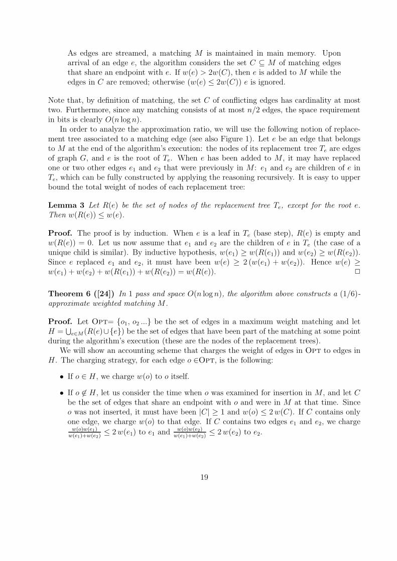
As edges are streamed, a matching M is maintained in main memory. Uponarrival of an edge e, the algorithm considers the set C ⊆ M of matching edgesthat share an endpoint with e. If w(e) > 2w(C), then e is added to M while theedges in C are removed; otherwise (w(e) ≤ 2w(C)) e is ignored.

Note that, by definition of matching, the set C of conflicting edges has cardinality at mosttwo. Furthermore, since any matching consists of at most n/2 edges, the space requirementin bits is clearly O(n logn).

In order to analyze the approximation ratio, we will use the following notion of replace-ment tree associated to a matching edge (see also Figure 1). Let e be an edge that belongsto M at the end of the algorithm’s execution: the nodes of its replacement tree Te are edgesof graph G, and e is the root of Te. When e has been added to M , it may have replacedone or two other edges e1 and e2 that were previously in M : e1 and e2 are children of e inTe, which can be fully constructed by applying the reasoning recursively. It is easy to upperbound the total weight of nodes of each replacement tree:

Lemma 3 Let R(e) be the set of nodes of the replacement tree Te, except for the root e.Then w(R(e)) ≤ w(e).

Proof. The proof is by induction. When e is a leaf in Te (base step), R(e) is empty andw(R(e)) = 0. Let us now assume that e1 and e2 are the children of e in Te (the case of aunique child is similar). By inductive hypothesis, w(e1) ≥ w(R(e1)) and w(e2) ≥ w(R(e2)).Since e replaced e1 and e2, it must have been w(e) ≥ 2 (w(e1) + w(e2)). Hence w(e) ≥w(e1) + w(e2) + w(R(e1)) + w(R(e2)) = w(R(e)). 2

Theorem 6 ([24]) In 1 pass and space O(n log n), the algorithm above constructs a (1/6)-approximate weighted matching M .

Proof. Let Opt= o1, o2 ... be the set of edges in a maximum weight matching and letH =

⋃e∈M(R(e)∪e) be the set of edges that have been part of the matching at some point

during the algorithm’s execution (these are the nodes of the replacement trees).We will show an accounting scheme that charges the weight of edges in Opt to edges in

H . The charging strategy, for each edge o ∈Opt, is the following:

• If o ∈ H , we charge w(o) to o itself.

• If o 6∈ H , let us consider the time when o was examined for insertion in M , and let Cbe the set of edges that share an endpoint with o and were in M at that time. Sinceo was not inserted, it must have been |C| ≥ 1 and w(o) ≤ 2 w(C). If C contains onlyone edge, we charge w(o) to that edge. If C contains two edges e1 and e2, we charge

w(o)w(e1)w(e1)+w(e2)

≤ 2 w(e1) to e1 and w(o)w(e2)w(e1)+w(e2)

≤ 2 w(e2) to e2.

19

(c)

120

130 40

1062 30

2

504

a b c

d fe

g h i

a b c

d fe

g h i

(f)

(a)

120

130 40

1062 30

2

504

a b c

d fe

g h i

(c,f)(b,e)

(e,f)

(d,e)

(d,g) (h,i)

(d)

(c,f,2)(b,e,10)(h,i,4)(e,f,30)(h,f,50)(e,g,40)(d,e,62)(a,d,120)(d,g,130)

(b)

Σ =

a b c

d fe

g h i

(e)

Figure 1: (a) A weighted graph and an optimal matching Opt (bold edges); (b) order inwhich edges are streamed; (c) matching M computed by the algorithm (bold solid edges)and edges in the history H \ M (dashed edges); (d) replacement trees of edges in M ; (e)initial charging of the weights of edges in Opt; (f) charging after the redistribution.

The following two properties hold: (a) the charge of o to any edge e is at most 2 w(e); (b) anyedge of H is charged by at most two edges of Opt, one per endpoint. (See also Figure 1.)

We now redistribute some charges as follows: if an edge o ∈Opt charges an edge e ∈ Hand e gets replaced at some point by an edge e′ ∈ H which also shares an endpoint witho, we transfer the charge of o from e to e′. With this procedure, property (a) remains validsince w(e′) ≥ w(e). Moreover, o will always charge an incident edge, and thus property (b)remains also true. In particular, each edge e ∈ H \ M will be now charged by at most oneedge in Opt: if at some point there are two edges charging e, the charge of one of them willbe transferred to the edge of H that replaced e. Thus, only edges in M can be charged bytwo edges in Opt. By the above discussion we get:

w(Opt) ≤∑

e∈H\M

2w(e) +∑

e∈M

4w(e) =∑

e∈M

2w(R(e)) +∑

e∈M

4w(e) ≤∑

e∈M

6w(e) = 6w(M)

where the first equality is by definition of H and the last inequality is by Lemma 3. 2

3.4 Simulation of PRAM algorithms

In this section we show that a variety of problems for which efficient solutions in classicalstreaming are not known or impossible can be solved very efficiently in the stream-sortmodel discussed in Section 2.3. In particular, we show that parallel algorithms designed in

20

the PRAM model [44] can yield very efficient algorithms in the stream-sort model. Thistechnique is very similar to previous methods developed in the context of external memorymanagement for deriving I/O efficient algorithms (see, e.g., [16]).

Theorem 7 Let A be a PRAM algorithm that uses N processors and runs in time T . ThenA can be simulated in stream-sort in p = O(T ) passes and space s = O(log N).

Proof. Let Σ = (1, val1)(2, val2) · · · (M, valM) be the input stream that represents thememory image given as input to algorithm A, where valj is the value contained at address j,and M = O(N). At each step of algorithm A, processor pi reads one memory cell at addressini, updates its internal state sti, and possibly writes one output cell at address outi. In apreprocessing pass, we append to Σ the N tuples:

(p1, in1, st1, out1) · · · (pN , inN , stN , outN)

where ini and outi are the cells read and written by pi at the first step of algorithm A,respectively, and sti is the initial state of pi. Each step of A can be simulated by performingthe following sorting and scanning passes:

1. We sort the stream so that each (j, valj) is immediately followed by tuples (pi, ini, sti, outi)such that ini = j, i.e., the stream has the form

(1, val1)(pi11 , 1, sti11, outi11)(pi12 , 1, sti12, outi12) · · ·(2, val2)(pi21 , 2, sti21, outi21)(pi22 , 2, sti22, outi22) · · ·. . .(M, valM)(piM1

, M, stiM1, outiM1

)(piM2, M, stiM2

, outiM2) · · ·

This can be done, e.g., by using 2j as sorting key for tuples (j, valj) and 2ini + 1 assorting key for tuples (pi, ini, sti, outi).

2. We scan the stream, performing the following operations:

• If we read (j, valj), we let currval = valj and we write (j, valj ,“old”) to theoutput stream.

• If we read (pi, ini, sti, outi), we simulate the task performed by processor pi, ob-serving that the value valini

that pi would read from cell ini is readily availablein currval. Then we write to the output stream (outi, resi,“new”), where resi isthe value that pi would write at address outi, and we write tuple (pi, in

′i, st

′i, out′i),

where in′i and out′i are the cells to be read and written at the next step of A,

respectively, and st′i is the new state of processor pi.

3. Notice that at this point, for each j we have in the stream a triple of the form(j, valj ,“old”), which contains the value of cell j before the parallel step, and pos-sibly one or more triples (j, resi,“new”), which store the values written by processorsto cell j during that step. If there is no “new” value for cell j, we simply drop the “old”

21

tag from (j, valj ,“old”). Otherwise, we keep for cell j one of the new triples prunedof the “new” tag, and get rid of the other triples. This can be easily done with onesorting pass, which lets triples by the same j be consecutive, followed by one scanningpass, which removes tags and duplicates.

To conclude the proof, we observe that, if A performs T steps, then our stream-sort simulationrequires p = O(T ) passes. Furthermore, the number of bits of working memory required toperform each processor task simulation and to store currval is s = O(log N). 2

Theorem 7 provides a systematic way of constructing streaming algorithms (in the stream-sortmodel) for several fundamental problems. Prominent examples are list ranking, Euler tour,graph connectivity, minimum spanning tree, biconnected components, and maximal inde-pendent set, among others [44], essentially matching the results obtainable in more powerfulcomputational models for massive data sets, such as the parallel disk model [58]. As observedby Aggarwal et al. [3], this suggests that using more powerful, harder to implement modelsmay not always be justified.

4 Lower bounds

An important technique for proving streaming lower bounds is based on communicationcomplexity lower bounds [40]. A crucial restriction in accessing a data stream is that itemsare revealed to the algorithm sequentially. Suppose that the solution of a computationalproblem needs to compare two items directly; one may argue that, if the two items are farapart in the stream, one of them must be kept in main memory for long time by the algorithmuntil the other item is read from the stream. Intuitively, if we have limited space and manydistant pairs of items to be compared, then we cannot hope to solve the problem unless weperform many passes over the data. We formalize this argument by showing reductions ofcommunication problems to streaming problems. This allows us to prove lower bounds instreaming based on communication complexity lower bounds. To illustrate this technique,we prove a lower bound for the element distinctness problem, which clearly implies a lowerbound for the computation of the number or distinct items F0 addressed in Section 3.2.

Theorem 8 Any deterministic or randomized algorithm that decides whether a stream of nitems contains any duplicates requires p = Ω(n/s) passes using s bits of working memory.

Proof. The proof follows from a two-ways communication complexity lower bound for thebit-vector-disjointness problem. In this problem, Alice has an n-bit-vector A and Bob hasan n-bit-vector B. They want to know whether A ·B > 0, i.e., whether there is at least oneindex i ∈ 1, . . . , n such that A[i] = B[i] = 1. By a well known communication complexitylower bound [45], Alice and Bob must communicate Ω(n) bits to solve the problem. Thisresults holds also for randomized protocols: any algorithm that outputs the correct answerwith high probability must communicate Ω(n) bits.

We now show that bit-vector-disjointness can be reduced to the element distinctnessstreaming problem. The reduction works as follows. Alice creates a stream of items SA

22

containing indices i such that A[i] = 1. Bob does the same for B, i.e., he creates a streamof items SB containing indices i such that B[i] = 1. Alice runs a streaming algorithm forelement distinctness on SA, then she sends the content of her working memory to Bob. Bobcontinues to run the same streaming algorithm starting from the memory image receivedfrom Alice, and reading items from the stream SB. When the stream is over, Bob sendshis memory image back to Alice, who starts a second pass on SA, and so on. At each pass,they exchange 2s bits. At the end of the last pass, the streaming algorithm can answerwhether the stream obtained by concatenating SA and SB contains any duplicates; since thisstream contains duplicates if and only if A · B > 0, this gives Alice and Bob a solution tothe problem.

Assume by contradiction that the number of passes performed by Alice and Bob overthe stream is o(n/s). Since at each pass they communicate 2s bits, then the total numberof bits sent between them over all passes is o(n/s) · 2s = o(n), which is a contradiction asthey must communicate Ω(n) bits as noticed above. Thus, any algorithm for the elementdistinctness problem that uses s bits of working memory requires p = Ω(n/s) passes. 2

Lower bounds established in this way are information-theoretic, imposing no restrictions onthe computational power of the algorithms. The general idea of reducing a communicationcomplexity problem to a streaming problem is very powerful, and allows it to prove severalstreaming lower bounds. Those range from computing statistical summary information suchas frequency moments [5], to graph problems such as vertex connectivity [40], and implythat for many fundamental problems there are no one-pass exact algorithms with a workingmemory significantly smaller than the input stream.

A natural question is whether approximation can make a significant difference for thoseproblems, and whether randomization can play any relevant role. An interesting observationis that there are problems such as the computation of frequency moments for which neitherrandomization nor approximation are powerful enough for getting a solution in one pass andsublinear space, unless they are used together.

4.1 Randomization

As we have seen in the proof of Theorem 8, lower bounds based on the communicationcomplexity of the bit-vector-disjointness problem hold also for randomized algorithms, whichyields clear evidence that randomization without approximation may not help. The resultof Theorem 8 can be generalized for all one-pass frequency moments. In particular, it ispossible to prove that any randomized algorithm for computing the frequency moments thatoutputs the correct result with probability higher than 1

2in one pass must use Ω(n) bits of

working memory. The theorem can be proven using communication complexity tools.

Theorem 9 ([6]) For any nonnegative integer k 6= 1, any randomized algorithm that makesone pass over a sequence of at least 2n items drawn from the universe U = 1, 2, . . . , n andcomputes Fk exactly with probability > 1

2must use Ω(n) bits of working memory.

23

4.2 Approximation

Conversely, we can show that any deterministic algorithm for computing the frequency mo-ments that approximates the correct result within a constant factor in one pass must useΩ(n) bits of working memory. Differently from the lower bounds addressed earlier in thissection, we give a direct proof of this result without resorting to communication complexityarguments.

Theorem 10 ([6]) For any nonnegative integer k 6= 1, any deterministic algorithm thatmakes one pass over a sequence of at least n/2 items drawn from the universe U = 1, 2, . . . , nand computes a number Y such that |Y − Fk| ≤ Fk

10must use Ω(n) bits of working memory.

Proof. The idea of the proof is to show that, if the working memory is not large enough,for any deterministic algorithm (which does not use random bits) there exist two subsets S1

and S2 in a suitable collection of subsets of U such that the memory image of the algorithmis the same after reading either S1 or S2, i.e., they are indistinguishable. As a consequence,the algorithm has the same memory image after reading either S1 ·S1 or S2 ·S1, where A ·Bdenotes the stream of items that starts with the items of A and ends with the items of B. IfS1 and S2 have a small intersection, then the two streams S1 ·S1 and S2 ·S1 must have ratherdifferent values of Fk, and the algorithm must necessarily make a large error on estimatingFk on at least one of them.

In more detail, using a standard construction in coding theory, it is possible to build afamily F of 2Ω(n) subsets of U of size n/4 each such that any two of them have at most n/8common items. Fix a deterministic algorithm and let s < Ω(n) be the size of its workingmemory. Since the memory can assume at most 2s different configurations and we have2Ω(n) > 2s possible distinct input sets in F , then by the pigeonhole principle there must betwo input sets S1, S2 ∈ F such that the memory image of the algorithm after reading eitherone of them is the same. Now, if we consider the two streams S1 ·S1 and S2 ·S1, the memoryimage of the algorithm after processing either one of them is the same. Since by constructionof F , S1 and S2 contain n/4 items each, and have at most n/8 items in common, then:

• Each of the n/4 distinct items in S1 · S1 has frequency 2, thus:

F S1·S1

k =n∑

i=1

fki = 2k · n

4.

• There are at least n8

+ n8

= n4

items in S2 · S1 with frequency 1 and at most n8

itemswith frequency 2, thus:

F S2·S1

k =n∑

i=1

fki ≤ n

4+ 2k · n

8.

Notice that the maximum error performed by the algorithm on either input S1 · S1 or inputS2 · S1 is minimized if the returned number Y is half way from F S1·S1

k and F S2·S1

k , i.e.,

24

|Y − F S1·S1

k | = |Y − F S2·S1

k | = |F S1·S1

k − F S2·S1

k |/2. With simple calculations, it is easy tocheck that:

|F S1·S1

k − F S2·S1

k |/2 >1

10· F S1·S1

k and |F S1·S1

k − F S2·S1

k |/2 >1

10· F S2·S1

k .

This implies that, if we use fewer than Ω(n) memory bits, there is an input on which thealgorithm outputs a value Y such that |Y − Fk| > Fk

10, which proves the claim. 2

4.3 Randomization and approximation

A natural approach that combines randomization and approximation would be to use randomsampling to get an estimator of the solution. Unfortunately, this may not always work: asan example, Charikar et al. [12] have shown that estimators based on random sampling donot yield good results for F0.

Theorem 11 ([12]) Let E be a (possibly adaptive and randomized) estimator of F0 thatexamines at most r items in a set of n items and let err = max E

F0

, F0

E be the error or the

estimator. Then for any p > 1er there is a choice of the set of items such that err ≥

√n−r2r

ln 1p

with probability at least p.

The result of Theorem 11 states that no good estimator can be obtained if we only examine afraction of the input. On the other hand, as we have seen in Section 3.2, hashing techniquesthat examine all items in the input allow it to estimate F0 within an arbitrary fixed errorbound with high probability using polylogarithmic working memory space for any given dataset.

We notice that, while the ideal goal of a streaming algorithm is to solve a problem usinga working memory of size polylogarithmic in the size of the input stream, for some problemsthis is impossible even using approximation and randomization, as shown in the followingtheorem from [6].

Theorem 12 ([6]) For any fixed integer k > 5, any randomized algorithm that makes onepass over a sequence of at least n items drawn from the universe U = 1, 2, . . . , n andcomputes an approximate value Y such that |Y − Fk| > Fk

10with probability < 1

2requires at

least Ω(n1−5/k) memory bits.

Theorem 12 holds in a streaming scenario where items are revealed to the algorithm in anon-line manner and no assumptions are made on the input. We finally notice that in thesame scenario there are problems for which approximation and randomization do not helpat all. A prominent example is given by the computation of F∞, the maximum frequency ofany item in the stream.

Theorem 13 ([6]) Any randomized algorithm that makes one pass over a sequence of atleast 2n items drawn from the universe U = 1, 2, . . . , n and computes an approximatevalue Y such that |Y − F∞| ≥ F∞

3with probability < 1

2requires at least Ω(n) memory bits.

25

5 Conclusions

In this chapter we have addressed the emerging field of data stream algorithmics, provid-ing an overview of the main results in the literature and discussing computational models,applications, lower bound techniques and tools for designing efficient algorithms. Severalimportant problems have been proven to be efficiently solvable despite the strong restric-tions on the data access patterns and memory requirements of the algorithms that arise instreaming scenarios. One prominent example is the computation of statistical summariessuch as frequency moments, histograms, and wavelet coefficient, of great importance in avariety of applications including network traffic analysis and database optimization. Otherwidely studied problems include norm estimation, geometric problems such as clustering andfacility location, and graph problems such as connectivity, matching, and distances.

From a technical point of view, we have discussed a number of important tools for de-signing efficient streaming algorithms, including random sampling, probabilistic counting,hashing, and linear projections. We have also addressed techniques for graph problems andwe have shown that extending the streaming paradigm with a sorting primitive yields enoughpower for solving a variety of problems in external memory, essentially matching the resultsobtainable in more powerful computational models for massive data sets.

Finally, we have discussed lower bound techniques, showing that tools from the field ofcommunication complexity can be effectively deployed for proving strong streaming lowerbounds. We have discussed the role of randomization and approximation, showing that forsome problems neither one of them yields enough power, unless they are used together. Wehave also shown that other problems are intrinsically hard in a streaming setting even usingapproximation and randomization, and thus cannot be solved efficiently unless we considerless restrictive computational models.

References

[1] D. Agrawal A. Metwally and A. El Abbadi. Efficient computation of frequent and top-kelements in data stream. In Proceedings ICDT, pages 398–412, 2005.

[2] J. Abello, A. Buchsbaum, and J. R. Westbrook. A functional approach to externalgraph algorithms. Algorithmica, 32(3):437–458, 2002.

[3] G. Aggarwal, M. Datar, S. Rajagopalan, and M. Ruhl. On the streaming model aug-mented with a sorting primitive. In Proceedings of the 45th Annual IEEE Symposiumon Foundations of Computer Science (FOCS), 2004.

[4] N. Alon, P. Gibbons, Y. Matias, and M. Szegedy. Tracking join and self-join sizes inlimited storage. In Proc. ACM PODS, pages 10–20. ACM Press, 1999.

[5] N. Alon, Y. Matias, and M. Szegedy. The space complexity of approximating thefrequency moments. In Proceedings of the 28th annual ACM Symposium on Theory ofComputing (STOC’96), pages 20–29. ACM Press, 1996.

26

[6] N. Alon, Y. Matias, and M. Szegedy. The space complexity of approximating thefrequency moments. Journal of Computer and System Sciences, 58(1):137–147, 1999.

[7] B. Babcock, S. Babu, M. Datar, R. Motwani, and J. Widom. Models and issues in datastream systems. In Proceedings of the 21st ACM Symposium on Principles of DatabaseSystems (PODS), pages 1–16, 2002.

[8] B. Babcock, M. Datar, and R. Motwani. Sampling from a moving window over streamingdata. In SODA, pages 633–634, 2002.

[9] Z. Bar-Yossef, T. Jayram, R. Kumar, and D. Sivakumar. Information statistics approachto data stream and communication complexity. In Proc. IEEE FOCS, 2002.

[10] Z. Bar-Yossef, R. Kumar, and D. Sivakumar. Reductions in streaming algorithms,with an application to counting triangles in graphs. In Proceedings of the thirteenthannual ACM-SIAM symposium on Discrete algorithms (SODA 2002), San Francisco,California, pp. 623-632, 2002.

[11] A. Chakrabarti, S. Khot, and X. Sun. Near-optimal lower bounds on the multi-partycommunication complexity of set disjointness. In Proc. IEEE Conference on Computa-tional Complexity, pages 107–117, 2003.

[12] M. Charikar, S. Chaudhuri, R. Motwani, and V. Narasayya. Towards estimation er-ror guarantees for distinct values. In PODS ’00: Proceedings of the nineteenth ACMSIGMOD-SIGACT-SIGART symposium on Principles of database systems, pages 268–279, New York, NY, USA, 2000. ACM Press.

[13] M. Charikar, K. Chen, and M. Farach-Colton. Finding frequent items in data streams.In Proc. ICALP, pages 693–703, 2002.

[14] M. Charikar, L. O’Callaghan, and R. Panigrahy. Better streaming algorithms for clus-tering problems. In Proc. ACM STOC, 2003.

[15] S. Chaudhuri, R. Motwani, and V. Narasayya. Random sampling for histogram con-struction: How much is enough? In Proc. SIGMOD, pages 436–447, 1998.

[16] Y. Chiang, M.T. Goodrich, E.F. Grove, R. Tamassia, D.E. Vemgroff, and J.S. Vitter.External-memory graph algorithms. In Proc. 6th Annual ACM-SIAM Symposium onDicrete Algorithms (SODA’95), pages 139–149, 1995.

[17] D. Coppersmith and R. Kumar. An improved data stream algorithm for frequencymoments. In Proc. ACM-SIAM SODA, pages 151–156, 2004.

[18] G. Cormode and S. Muthukrishnan. Estimating dominance norms on multiple datastreams. In European Symposium on Algorithms (ESA), pages 148–160, 2003.

27

[19] G. Cormode and S. Muthukrishnan. What is hot and what is not: Tracking mostfrequent items dynamically. In ACM PODS, 2003.

[20] G. Cormode and S. Muthukrishnan. An improved data stream summary: the count-minsketch and its applications. J. Algorithms, 55(1):58–75, 2005.

[21] G. Cormode and S. Muthukrishnan. Space efficient mining of multigraph streams. InACM PODS, 2005.

[22] C. Demetrescu, I. Finocchi, and A. Ribichini. Trading off space for passes in graphstreaming problems. In Proc. 17th ACM-SIAM SODA, pages 714–723, 2006.

[23] M. Elkin and J. Zhang. Efficient algorithms for constructing (1 + ǫ, β)-spanners in thedistributed and streaming models. In Proc. ACM PODC, pages 160–168, 2004.

[24] J. Feigenbaum, S. Kannan, A. McGregor, S. Suri, and J. Zhang. On graph problemsin a semi-streaming model. In Proc. of the International Colloquium on Automata,Languages and Programming (ICALP), 2004.

[25] J. Feigenbaum, S. Kannan, A. McGregor, S. Suri, and J. Zhang. Graph distances in thestreaming model: the value of space. In Proceedings of the 16th ACM/SIAM Symposiumon Discrete Algorithms (SODA), pages 745–754, 2005.

[26] P. Flajolet and G. N. Martin. Probabilistic counting. In Proceedings of the 24th AnnualSymposium on Foundations of Computer Science, 7-9 November 1983, Tucson, Arizona,USA, pages 76–82, 1983.

[27] P. Flajolet and G. N. Martin. Probabilistic counting algorithms for data base applica-tions. J. Comput. Syst. Sci., 31(2):182–209, 1985.

[28] G. Frahling, P. Indyk, and C. Sohler. Sampling in dynamic data streams and applica-tions. In Proc. 21st ACM Symposium on Computational Geometry, pages 79–88, 2005.

[29] G. Frahling and C. Sohler. Coresets in dynamic geometric data streams. In Proc. 37thACM STOC, 2005.

[30] P. B. Gibbons and Y. Matias. New sampling-based summary statistics for improvingapproximate query answers. In Proceedings ACM SIGMOD, 1998.

[31] P. B. Gibbons and Y. Matias. Synopsis data structures for massive data sets. In “Ex-ternal Memory algorithms”, DIMACS series in Discrete Mathematics and TheoreticalComputer Science, 50:39–70, 1999.

[32] P. B. Gibbons, Y. Matias, and V. Poosala. Fast incremental maintenance of approximatehistograms. In Proceedings 23rd VLDB, 1997.

[33] A. Gilbert, Y. Kotidis, S. Muthukrishnan, and M. Strauss. How to summarize theuniverse: Dynamic maintenance of quantiles. In Proc. VLDB, pages 454–465, 2002.

28

[34] A. C. Gilbert, S. Guha, P. Indyk, Y. Kotidis, S. Muthukrishnan, and M. Strauss. Fast,small-space algorithms for approximate histogram maintenance. In Proceedings of the34th ACM Symposium on Theory of Computing (STOC), pages 389–398, 2002.

[35] A. C. Gilbert, Y. Kotidis, S. Muthukrishnan, and M. Strauss. Surfing wavelets onstreams: One-pass summaries for approximate aggregate queries. In Proc. 27th Int.Conf. on Very Large Data Bases (VLDB), pages 79–88, 2001.

[36] L. Golab and M. T. Ozsu. Data stream management issues a survey. Technical report,School of Computer Science, University of Waterloo, TR CS-2003-08, 2003.

[37] S. Guha, P. Indyk, S. Muthukrishnan, and M. Strauss. Histogramming data streamswith fast per-item processing. In Proc. ICALP, pages 681–692, 2002.

[38] S. Guha, N. Koudas, and K. Shim. Data streams and histograms. In Proc. ACM STOC,pages 471–475, 2001.

[39] S. Guha, N. Mishra, R. Motwani, and L. O’Callaghan. Clustering data streams. InProc. IEEE FOCS, pages 359–366, 2000.

[40] M. Henzinger, P. Raghavan, and S. Rajagopalan. Computing on data streams. In “Ex-ternal Memory algorithms”, DIMACS series in Discrete Mathematics and TheoreticalComputer Science, 50:107–118, 1999.

[41] P. Indyk. Stable distributions, pseudorandom generators, embeddings and data streamcomputation. In Proc. 41st IEEE FOCS, pages 189–197, 2000.

[42] P. Indyk. Algorithms for dynamic geometric problems over data streams. In Proc. ACMSTOC, pages 373–380, 2004.

[43] P. Indyk and D. Woodruff. Tight lower bounds for the distinct elements problem. InProc. IEEE FOCS, 2003.

[44] J. Jaja. An introduction to parallel algorithms. Addison-Wesley, 1992.

[45] E. Kushilevitz and N. Nisan. Communication Complexity. Cambridge University Press,1997.

[46] G. S. Manku and R. Motwani. Approximate frequency counts over data streams. InProceedings 28th Int. Conference on Very Large Data Bases (VLDB 2002), pages 346–357. Morgan Kaufmann, 2002.

[47] Y. Matias, J. S. Vitter, and M. Wang. Dynamic maintenance of wavelet-based his-tograms. In Proceedings 26th VLDB, 2000.

[48] A. McGregor. Finding matchings in the streaming model. In Proceedings of the 8thInternational Workshop on Approximation Algorithms for Combinatorial OptimizationProblems (APPROX 2005), LNCS 3624, pages 170–181, 2005.

29

[49] J. Misra and D. Gries. Finding repeated elements. Science of Computer Programming,2:143–152, 1982.

[50] I. Munro and M. Paterson. Selection and sorting with limited storage. TheoreticalComputer Science, 12:315–323, 1980.

[51] S. Muthukrishnan. Data streams: algorithms and applications. Technical report, 2003.Available at http://athos.rutgers.edu/∼muthu/stream-1-1.ps.

[52] S. Muthukrishnan and M. Strauss. Maintenance of multidimensional histograms. InProc. FSTTCS, pages 352–362, 2003.

[53] S. Muthukrishnan and M. Strauss. Rangesum histograms. In Proc. ACM-SIAM SODA,2003.

[54] S. Muthukrishnan and M. Strauss. Approximate histogram and wavelet summaries ofstreaming data. Technical report, 2004. DIMACS TR 2004-52.

[55] M. Ruhl. Efficient Algorithms for New Computational Models. PhD thesis, Departmentof Electrical Engineering and Computer Science, Massachusetts Institute of Technology,2003.

[56] M. Saks and X. Sun. Space lower bounds for distance approximation in the data streammodel. In Proc. ACM STOC, pages 360–369, 2002.

[57] J. S. Vitter. Random sampling with a reservoir. ACM Transactions on MathematicalSoftware, 11(1):37–57, March 1985.

[58] J. S. Vitter. External memory algorithms and data structures: Dealing with massivedata. ACM Computing Surveys, 33(2):209–271, 2001.

30