Larrosa, N. (2017). 'Mind the Gap' in Fitness-For-Service AssessmentProcedures-Review and Summary of a Recent Workshop. InternationalJournal of Pressure Vessels and Piping.https://doi.org/10.1016/j.ijpvp.2017.09.004

Peer reviewed version

Link to published version (if available):10.1016/j.ijpvp.2017.09.004

Link to publication record in Explore Bristol ResearchPDF-document

This is the author accepted manuscript (AAM). The final published version (version of record) is available onlinevia ELSEVIER at http://www.sciencedirect.com/science/article/pii/S0308016117301205. Please refer to anyapplicable terms of use of the publisher.

University of Bristol - Explore Bristol ResearchGeneral rights

This document is made available in accordance with publisher policies. Please cite only the publishedversion using the reference above. Full terms of use are available:http://www.bristol.ac.uk/pure/about/ebr-terms

Accepted Manuscript

‘Mind the gap’ in fitness-for-service assessment procedures-review and summary of arecent workshop

N.O. Larrosa, R.A. Ainsworth, R. Akid, P.J. Budden, C.M. Davies, I. Hadley, D.R.Tice, A. Turnbull, S. Zhou

PII: S0308-0161(17)30120-5

DOI: 10.1016/j.ijpvp.2017.09.004

Reference: IPVP 3649

To appear in: International Journal of Pressure Vessels and Piping

Received Date: 25 March 2017

Revised Date: 26 September 2017

Accepted Date: 30 September 2017

Please cite this article as: Larrosa NO, Ainsworth RA, Akid R, Budden PJ, Davies CM, Hadley I, TiceDR, Turnbull A, Zhou S, ‘Mind the gap’ in fitness-for-service assessment procedures-review andsummary of a recent workshop, International Journal of Pressure Vessels and Piping (2017), doi:10.1016/j.ijpvp.2017.09.004.

This is a PDF file of an unedited manuscript that has been accepted for publication. As a service toour customers we are providing this early version of the manuscript. The manuscript will undergocopyediting, typesetting, and review of the resulting proof before it is published in its final form. Pleasenote that during the production process errors may be discovered which could affect the content, and alllegal disclaimers that apply to the journal pertain.

MANUSCRIP

T

ACCEPTED

ACCEPTED MANUSCRIPT

1 Corresponding author e-mail: nicolas.larrosa@bristol.ac.uk

‘Mind the Gap’ in Fitness-For-Service Assessment Procedures-Review and Summary of a

Recent Workshop.

N.O. Larrosaa,b 1, R.A. Ainsworthc, R. Akida, P.J. Buddend,

C.M. Daviese, I. Hadleyf, D.R. Ticeg, A. Turnbull h and S. Zhou h

a School of Materials, The University of Manchester, Manchester, UK.

b Department of Mechanical Engineering, University of Bristol, Bristol, UK

c School of Mechanical, Aerospace & Civil Engineering, The University of Manchester, Manchester, United Kingdom.

d Assessment Technology Group, EDF Energy Barnwood, Gloucester, UK.

e Department of Mechanical Engineering, Imperial College London, London, UK.

f TWI, Abington Hall, Granta Park, Great Abington, UK

g AMEC Foster Wheeler, Birchwood, Warrington, UK

h National Physical Laboratory (NPL), Hampton Rd., Teddington, Middlesex, UK

Abstract

‘Mind the gap’ in Fitness-for-Service (FFS) assessment procedures was a workshop held at The University of Manchester in June 2015. The goal of the workshop was firstly to identify ‘knowledge gaps’ or areas for improvement in FFS assessment procedures and, secondly, to present methodologies that have been developed to narrow these gaps. It was intended that identification of these ‘gaps’ would allow an understanding of the current development needs for defect tolerance arguments in the FFS assessment procedures. The following questions were addressed: 1) What are the main ‘knowledge gaps’ in current FFS assessment procedures and methodologies? 2) What are the main barriers that need to be overcome in order to narrow these ‘gaps’? 3) What are the current procedures (if any) and why are these not useful, over- or under-conservative and what needs to be improved? 4) What research is currently ongoing in order to narrow the gaps? This paper summarises the presentations and discussions at the workshop on subjects such as environmentally assisted cracking mechanisms, creep, welding residual stresses and fracture mechanics.

Key words: Fitness-for-service, Assessment procedures, Knowledge gaps, Creep, Fracture, Corrosion fatigue, Environmentally assisted fatigue, Welding Residual Stresses

MANUSCRIP

T

ACCEPTED

ACCEPTED MANUSCRIPT

2

1 Introduction

Fitness-For-Service (FFS) assessment procedures provide standardised routes to assess the residual properties of an in-service structure in order to aid decisions regarding whether continued operation is acceptable, or whether repair or replacement is needed. Common FFS assessment procedures include the UK nuclear industry standards for creep and fracture assessment, R5 [1] and R6 [2], respectively, the American Petroleum Institute document API 579/ASME FFS-1 [3], the ASME Boiler and Pressure vessel Code and the British Standards Institution Guide BS 7910 [4]. FFS assessment procedures are based on simplified approaches, which lead to conservative assessments. For example: Part 6 in API 579/ASME FFS-1 and Annex G in BS7910, for assessing corrosion defects are based on local plastic collapse; ASME Sections III and XI provide procedures for fatigue design and fatigue crack growth, respectively. However, these procedures are not intended to cover applications where the component is subject to significant fatigue loading, or brittle fracture is likely to occur (even under static loading). Further, when a component is subject to the combined effects of cyclic loading and corrosion pitting, pits act as stress raisers that may become sites for crack initiation depending on the combination of mechanical and environmental factors. At present it is common to assume a detected pit is a sharp crack, as there is little guidance on how to deal with non-sharp defects from a fracture mechanics point of view. It is well known that assessing pits as cracks might be overly conservative. More generally, methods which account for the complex effects of environment on structural integrity often introduce high levels of conservatism.

It is commonly accepted that defects in most engineering components are subjected to less severe crack tip conditions (lower hydrostatic stresses and maximum principal stresses) than those in standard deeply cracked test specimens used to experimentally obtain the material‘s fracture toughness or to measure crack growth rates by creep, fatigue or stress corrosion cracking. This is done as it would not be possible to measure fracture toughness values specific to every structure (different shapes and sizes), loading and crack size of interest. This leads, however, in many cases to an underestimation of the material‘s capacity to resist fracture and the component's ability to withstand load.

The design and assessment of components operating in harsh environments for very long durations is traditionally based on design codes, such as the ASME Boiler and Pressure Vessel Code, and fitness-for-service approaches such as API 579/ASME FFS-1. These are often used in conjunction with data derived from short-term tests and therefore can involve highly conservative assumptions. API 579/ASME FFS-1, for example, uses simple creep deformation models and enhances creep crack growth rates using a creep damage model even though such damage effects may already be reflected in the measured creep crack growth data.

MANUSCRIP

T

ACCEPTED

ACCEPTED MANUSCRIPT

3

The estimation of welding residual stresses plays a major role in structural integrity assessment of welded structures. FFS assessment procedures use simplified approaches to include these stresses in the analysis and there are some differences between the residual stress profiles proposed in the FFS codes for certain cases. It is recognised that these procedures are not only overconservative in many cases but also underestimate residual stresses in other cases due to either limited measurement data or controlling parameters not clearly identified [5]. These techniques would need to be improved by mechanistic understanding and the implementation of appropriate measurement and modelling techniques.

Against this background, a workshop was organized and sponsored by The University of Manchester and the BP-International Centre for Advanced Materials and was held in Manchester, UK, on 1 June 2015. This paper presents the results of the workshop. The damage mechanisms of fracture, creep and corrosion and the estimation of residual stresses are discussed and research opportunities for the development of advanced procedures to overcome the ‘gaps’ identified are highlighted.

2 Summary of discussions on Fracture Mechanics

2.1 Applications and limitations of Engineering Critical Assessment (ECA) (Dr I. Hadley)

The UK FFS procedure BS 7910 [4] has grown considerably since its origins as the British Standards documents PD 6493:1980 ('Guidance on methods for assessing the acceptability of flaws in fusion welded structures') and PD 6539:1994 (‘Guide to methods for the assessment of the influence of crack growth on the significance of defects in components operating at high temperatures’). PD 6493:1980 was developed primarily as a tool for assessing the acceptability of fabrication flaws in welded structures, i.e. for deciding whether or not repair of a known flaw was required on the basis of fracture mechanics. Typically, this would be a flaw already considered unacceptable by the appropriate fabrication code, but difficult to repair. Consequently, the main requirement was for safety, i.e. the avoidance of failure. Safety margins against failure were known at the time to be both significant and variable, but the advantage of PD 6493 (later superseded by BS 7910) lay mainly in the fact that it allowed analyses to be carried out quickly (using parametric equations or graphical methods) and with limited input data. It therefore played an important role in the nascent UK offshore oil and gas industry, helping to ensure the safety and cost-effective installation and operation of offshore structures and process plant.

MANUSCRIP

T

ACCEPTED

ACCEPTED MANUSCRIPT

4

As confidence in the methods grew, so the procedure evolved to incorporate aspects of other procedures, in particular R6 [2]. This allowed fracture analysis to be presented in terms of a Failure Assessment Diagram (FAD), and the level of analysis to be tuned to the data available. PD 6493 was re-badged as BS 7910, and became increasingly used for purposes such as the assessment of in-service flaws, failure investigation, and for setting NDT flaw acceptance criteria. This last application is sometimes termed as ‘design ECA’, i.e. it is based on the assumption that a flaw that could lead to failure during the life of the structure must be highly detectable.

In view of the increased demand on modern welded structures (due, for example, to the need to accommodate very high or low temperatures, plastic straining, thinner sections, higher-strength materials, sour service) there is now a need for more accurate ECA techniques, preferably incorporating known safety factors so that techniques such as probabilistic fracture mechanics can be used, coupled with risk/reliability concepts. The latest edition of BS 7910 aims to address this need by including new annexes addressing crack-tip constraint, welding residual stress distributions and weld strength mismatch, all of which can be used to improve the accuracy of the analysis of a known flaw, albeit at the cost of generating significant amounts of new input data. Techniques such as finite element analysis can also be used to address geometries and loading conditions not adequately covered by the idealised models in BS 7910. With progressive improvements in input data and assessment procedure, the accuracy of the analysis of known flaws can be improved using BS 7910:2013 in place of earlier editions, as shown by a number of published examples [6], and there is an expectation by industry that the same principles can be applied to ECA at the design stage.

However, when the analysis procedure is ’reverse-engineered’ to set NDT acceptance criteria, i.e. to inform the design of a welded structure, it can be difficult to take advantage of the more advanced features of ECA. One example is the use of ECA to set inspection criteria for defects in the girth welds of offshore pipelines, where the requirements include speed of analysis, adjustment of the results to take account of NDT reliability, and simple acceptance criteria that can be applied on a lay-barge. Inspection is typically carried out using Automated Ultrasonic Testing (AUT), allowing a direct estimate of flaw height.

An example of a typical scenario analysed during pipeline ECA is shown in Fig. 1. Five hypothetical flaws of similar size but in different locations are shown; three are surface-breaking (S1-S3) and two embedded (E1-E2), but with different ligament heights, p1 and p2. A ‘known flaw’ assessment could take account of the microstructure at the crack tip (weld metal, HAZ or parent metal) and the location of the flaw relative to the surface and to stress-concentrating regions such as the weld toe. A more advanced assessment using the latest features of BS 7910:2013 might also be able to account for the residual stress at the crack tip, the difference in tensile properties between weld metal and parent metal and even the crack tip constraint

MANUSCRIP

T

ACCEPTED

ACCEPTED MANUSCRIPT

5

conditions (during installation, pipelines are subjected to loading under predominantly tensile conditions, in contrast with fracture mechanics test specimens, which are usually tested under conditions of in-plane bending). However, detection, sizing, location and analysis of flaws on a case-by-case basis during pipe laying would be an unimaginably slow process. Instead, the pipeline ECA aims to provide a single acceptance criterion for all flaws, based on combining the highest credible driving force with the lowest fracture toughness of the weldment. The result is a single locus of tolerable flaw sizes output from the ECA (see Fig. 2), which is shifted downwards to take account of the limitations of flaw sizing, then simplified to allow rapid sentencing of flaws on the lay-barge.

Figure 1 Example of narrow-gap girth weld showing possible locations of flaws

To summarise, there is certainly scope for improving the ECA of pipeline girth welds, which could in turn lead to a lower repair rate whilst maintaining structural integrity, but project timescales typically preclude this; the final ECA can only be carried out once the pipe has been procured and the weld procedure qualification and fracture toughness tests completed. Moreover, inspection qualification and ECA are intimately linked, so a change in flaw acceptance criteria could lead to a requirement for requalification of the AUT. Improvements will therefore only be achieved through research and development carried out away from the critical path of an offshore pipeline construction project.

MANUSCRIP

T

ACCEPTED

ACCEPTED MANUSCRIPT

6

Figure 2 Output of pipeline ECA. Full yield residual stresses considered relaxing with increasing Lr as allowed for in BS 7910 (clause 7.1.8.2).

A second example of a ‘design ECA’ relates to calculating the defect-tolerance of fatigue-loaded structures that have initially been designed using fatigue design codes such as BS 7608 (‘Guide to fatigue design and assessment of steel products’). BS 7608 presents design rules for fatigue-loaded structures in the form of S-N curves, based on statistical analysis of fatigue test data obtained from tests on welded joints. A straight line relationship between log S and log N is assumed, where S = stress range and N = fatigue life. The resulting curves have the form SmN = A, where m is the slope and A is a constant. The final design curves are set below the mean S-N curves, usually two standard deviations of log N to give approximately 97.5% probability of survival.

For a so-called class E weld (such as a full-penetration butt weld) and a design life of 1 million cycles, the BS 7608 design curve (see Fig. 3) shows that it is safe to apply a stress range of 100MPa. At higher stress ranges and/or under a greater number of stress cycles, there is a risk of fatigue crack growth, typically starting at the weld toe. The design curve method assumes that there are no gross flaws at the weld toe (this is typically confirmed via surface inspection), although in practice there will be very small-scale discontinuities known as non-metallic intrusions which act as initiation points for fatigue crack growth. The exact depth of intrusions depends on the process used, but the range 0.1-0.4mm was established by sectioning of welds [2]. In practice, intrusions are considered to be 0.25mm deep and would not therefore be classified as defects during inspection.

MANUSCRIP

T

ACCEPTED

ACCEPTED MANUSCRIPT

7

Figure 3 Example of fatigue design curves (S-N curves)

For fatigue-critical structures that cannot be inspected during their lifetime (for example, offshore risers), operators may wish to augment the fatigue design calculation with a demonstration of defect-tolerance, i.e. to demonstrate that even if a flaw is missed during the initial pre-service inspection, it will not grow large enough to lead to failure within the design life of the structure. This would entail supplementing the BS 7608 design rules with a fatigue analysis to BS 7910, the latter starting from an initial flaw size that corresponds to a high probability of detection, and using the Paris law to estimate an upper-bound limit to crack growth. Using Annex T of BS 7910 (‘Guidance on the use of NDT with ECA’) and assuming the use of zonal AUT or magnetic particle inspection, the postulated flaw height should then be at least 1.5mm – an order of magnitude higher than the height of the weld toe intrusions.

The implications of this difference are illustrated in Fig. 4. This shows the predicted size of flaws with an initial height, ai, of 0.1mm, 0.25mm and 0.4mm (representing weld toe intrusions) in a 25mm thick plate over time. Final failure is assumed to occur by overload when the flaw height reaches 12.5mm (this size is arbitrary, but in practice makes little difference to the result). An upper bound fatigue crack growth rate in air is assumed (to harmonize with the assumptions made in deriving the

MANUSCRIP

T

ACCEPTED

ACCEPTED MANUSCRIPT

8

design rules), and it can be seen that crack height after the application of a million cycles ranges from negligible (for ai =0.1mm) to substantial (for ai=0.4mm), commensurate with the design rules for this type of joint.

Starting from a 1.5mm high macroscopic flaw under the same load cycle, the flaw reaches a height of 12.5mm (and hence failure) after just 300,000 cycles.

Figure 4 Example of the application of fracture mechanics to fatigue design

There is, of course, no easy solution to the question of how to incorporate ECA concepts at the design stage. A straightforward ‘reverse-engineering’ of an ECA procedure, using upper-bound estimates of stresses and flaw sizes combined with lower-bound estimates of toughness and tensile properties, could lead to the conclusion that the structure has zero defect-tolerance. Conversely, the deliberate choice of less conservative inputs in the ‘design ECA’ could lead to premature failure if, for example, the as-built properties of the structure are below the levels envisaged in the ECA. The important point is that analysts need to be aware of, and work around, the limitations of ECA in design. This might include: carrying out extensive sensitivity studies to investigate the impact of various design scenarios, carrying out a preliminary ECA based on design parameters (followed by a more detailed calculation when the full data are available) or the use of probabilistic techniques. It is intended that future editions of BS 7910 will address the distinction between use of ECA in analysis of a known flaw and use in design more explicitly.

MANUSCRIP

T

ACCEPTED

ACCEPTED MANUSCRIPT

9

2.2 Ductile Fracture: Some Recent Developments and Issues for FFS Procedures. (Prof R.A. Ainsworth)

Some issues in ductile fracture assessment are: allowing for loss of constraint; ductile fracture at blunt notches; and the influence of prior strains on ductile fracture toughness. These three issues are summarized in this section.

There are existing procedures for addressing constraint loss in procedures such as R6 [1], based on the work of Ainsworth and O’Dowd [6]. These procedures involve a number of steps, which are summarized as follows.

1. Measure the high constraint fracture toughness K mat using standard deeply cracked bend fracture specimens.

2. Evaluate the standard R6 parameters Kr and Lr for the defective component. 3. Perform a Failure Assessment Diagram (FAD) assessment using the standard

failure assessment curve, f (Lr ) . 4. Evaluate the structural constraint parameter, β, for the defective component.

Often, the elastic constraint parameter, βT = T /Lrσ yis used, where T is the T-

Stress 5. Using a range of test specimen geometries and crack sizes (e.g. SENT, shallow

cracked SENB), and hence a range of constraint levels, β, measure the low constraint toughness Kmat

c . 6. Fit the data from step 5 with a function, typically of the form

Kmatc = Kmat[1+ α(−βLr )

m].

7. Construct a constraint modified FAD using the failure assessment curve f (Lr )[1+ α(−βLr )

m] and compare the assessment point (Lr, Kr) for the defective component with this modified curve.

Figure 5 The standard FAD (red) and constraint based FAD (blue). The loading line (green) indicates the increased allowable load when using the constraint based FAD.

The process is illustrated in Figure 5 which shows the increased margins against fracture which are possible with the constraint-based method. Although this approach has been formulated for some time, it is not often used and most assessments stop at step 3 above, i.e. stop after performing a standard assessment.

MANUSCRIP

T

ACCEPTED

ACCEPTED MANUSCRIPT

10

One of the difficulties with the approach described above is that a number of different specimens or defect sizes are required at step 5 in order to generate the function of step 6, which is used to construct the constraint modified FAD. More recently, therefore, alternative approaches have been suggested [8, 9], which are targeted at the use of specimens which more closely match the specific constraint level of interest in the component being assessed. The steps in an alternative constraint approach are as follows.

1. Evaluate the standard R6 parameters Kr and Lr for the defective component, using the high constraint toughness, as in step 2 above.

2. Evaluate the structural constraint parameter, β, for the defective component, as in step 4 above.

3. Choose a test specimen geometry (e.g. SENT, SENB) and choose a representative thickness, based on the defective component dimensions.

4. Choose the relative crack size, a/W, in the test specimen so that is the same (or higher constraint) as that evaluated for the component in step 2.

5. Choose the test specimen width, W, so that the ratio (Kr/Lr) is the same (or higher) as that in the component.

6. Then it follows that the loading line on the FAD (i.e. the slope Kr/Lr) is the same in the test specimen and the component and so is the constraint modified FAD. Hence the values of Kr and Lr for the defective component at fracture are the same as in the chosen test specimen.

The application of this alternative constraint approach has been demonstrated in [8], where it has been shown that it can be successful but in some cases can require large test specimens, in which case the constraint based approach using a range of specimens is required.

Despite the existence of constraint based methods, their lack of widespread use means that further work is required to fill gaps to enable their use. Some areas requiring further work are:

• Availability and confidence in the accuracy of constraint parameters for practical cases: o T-stress solutions for complex geometries and loadings; o T-stress solutions for complex secondary stresses (e.g. described by weight

functions); o Q-stress solutions for complex cases and combined loadings for a range of

material strain hardening behaviours. • Availability of materials fracture toughness data and testing standards for low

constraint levels: o More use of low constraint geometries for material testing; o Confidence in ductile damage modelling to simulate data and fill gaps so

that only limited testing is required in step 5 of the first constraint approach above.

• Large-Scale Validation to give confidence in the overall approach. o This is, however, difficult to obtain particularly for combined loadings.

MANUSCRIP

T

ACCEPTED

ACCEPTED MANUSCRIPT

11

The second topic discussed here is the effect of notch root radius on ductile tearing resistance. In this case, some results from ductile damage modelling of CT specimens of four materials were presented [10] showing how the effective fracture toughness, both at initiation and the resistance curve, are increased with increasing notch radius. Some results are shown in Figure 6. More recently, experimental data have been presented, also demonstrating the increase in effective ductile fracture resistance with increasing notch radius [11,12].

Figure 6 Determination of effective initiation toughness as a function of notch radius: (a) API X65, (b) API X70, (c) alloy 617 and (d) SA508 Gr.3.

The increased toughness leads to FAD assessments of the CT specimens that tend towards plastic collapse failure with increasing notch radius, Figure 7.

MANUSCRIP

T

ACCEPTED

ACCEPTED MANUSCRIPT

12

Figure 7 Loci of assessment points with increasing load, for a range of notch radius: (a) API X65, (b) API X70, (c) alloy 617 and (d) SA508 Gr.3.

Both constraint loss and notch bluntness can be described by an increase in effective fracture toughness. Therefore, a pertinent question is whether the effect of notch root radius can be described in terms of a loss of constraint. Some preliminary work has shown that the tearing resistance curve of a blunt notch can be matched to that in a low constraint geometry (see Fig. 8) but further work is required to examine whether this can be generalised. If it can, then it provides an opportunity to treat constrain loss and notch bluntness with a unified approach. As with the work on loss of constraint, there are some gaps which need to be filled before assessments taking advantage of increased effective toughness can be routinely used, some of these are;

• Development of non-destructive techniques so that there is knowledge of notch radius in practical applications;

• Confidence in ductile damage modelling to generate relevant fracture toughness data to minimise testing requirements;

MANUSCRIP

T

ACCEPTED

ACCEPTED MANUSCRIPT

13

• Experimental standards for measuring notch fracture toughness; • Development of step-by-step assessment procedures for codes such as R6; • Experimental validation to convincingly demonstrate that the increased notch

toughness can be used.

Figure 8 Stress triaxiality and predicted J-R curves for notched and standard C(T) specimens in API X70.

The final topic discussed is how the fracture toughness may be influenced by the prior plastic straining, which may be induced by welding or by prior loading (e.g. a proof pressure test) and may occur before or after a crack is formed. Approximately uniform pre-strain may be expected if the prior loading occurs before a crack is formed. However, highly non-uniform pre-strain is likely if a component is already cracked at the time of the prior loading. Both of these may affect the effective fracture toughness. This may be allowed for directly by measuring the fracture toughness of weld metal or uniformly pre-strained material. However, plastic strains in parent metal may be significant adjacent to a weld, presenting testing difficulties. In addition, there may be effects of ageing and irradiation between a prior load and a maximum load experienced in service.

Studies on uniform pre-straining [13] and recent studies on highly non-uniform straining [14], such as occurs if a defect is present during the proof loading for example, have been performed.

A uniform prestrain reduces the remaining ductility and hardens the material, effectively increasing the yield stress and reducing the subsequent hardening. However, experimental evidence and modelling suggests the effects are small [13], with a potential small increase in fracture toughness for small plastic pre-strains and a potential reduction in fracture toughness for large plastic pre-strains.

MANUSCRIP

T

ACCEPTED

ACCEPTED MANUSCRIPT

14

A non-uniform prestrain reduces remaining ductility non-uniformly and is associated with high hydrostatic stresses (low ductility) near the crack tip. Equally, it hardens the material non-uniformly and may lead to some initial ductile crack growth. Therefore, a non-uniform prestrain may significantly complicate the measurement of representative fracture toughness values [14].

To treat these load history effects in assessments requires the following gaps to be filled:

o Development of simplified methods to conservatively address load-history effects, in particular to identify when they are important and when not;

o Generate confidence in ductile damage modelling, to include reverse loading effects on material properties and changes in material properties with time, to minimise testing requirements;

o Experimental data to provide validation for cases representative of those seen in practice.

2.3 R6 vs BS 7910 vs API 579/ASME FFS-1: Comparison and discussion of ECA example problems. (Dr N.O. Larrosa)

Using the Failure Assessment Diagrams (FAD), some similarities and differences in results for candidate problems assessed by the R6 [2], API 579/ASME FFS-1 [3] and BS 7910 [4] procedures are discussed here.

Example problems 9.5 and 9.6 from API 579-FFS2 [15] are used as benchmarks. Example problem 9.5 consists of a crack-like flaw parallel to a longitudinal double V-groove seam weld on the inside surface of a pipe under internal pressure, Fig. 9(a), whereas example problem 9.6 deals with a crack-like flaw in a circumferential seam on the outside surface of a pipe under internal pressure and global bending, Fig. 9(b).

When welding residual stresses are considered in an analysis, a significant impact on the assessment of the crack driving force (through the parameter Kr in the FAD) was observed. In order to account for the effect of welding residual stresses, the residual stress distribution is required as input to perform fitness-for service assessment of a component containing a crack-like flaw at a weld joint. Different levels (Options) of analysis to account for residual stresses are proposed in the standards. A significant dependency on the Option used to account for residual stresses was also observed (Table 1).

MANUSCRIP

T

ACCEPTED

ACCEPTED MANUSCRIPT

15

Figure 9 Geometries considered for the comparison of the FFS assessment procedures: (a) Problem 9.5 [14] 1; (b) Problem 9.6 [15]

Table 1 Assessment results for Problem 9.6[14]. Effect of ‘Level 1’ and ‘Level 2’ residual stress effect in Kr included. Percentage difference with respect to API 579/ASME FFS-1 estimation is shown in parenthesis.

Lr Kr

No Residual Stresses

API 579 0.3991 0.1189

R6 0.3163 (-20.75) 0.1213(1.97)

BS 7910 0.5170 (29.54) 0.0963 (-19.06)

Uniform Residual Stress profile (Level 1)

API 579 0.3991 0.4483

R6 0.3163 (-20.75) 0.3756(-16.23)

BS 7910 0.5170 (29.54) 0.4052 (-9.61)

Non-uniform Residual Stress profile (Level 2)

API 579 0.3991 0.2496

R6 0.3163 (-20.75) 0.1213(-51.40)

BS 7910 0.5170 (29.54) 0.0963 (-61.42)

For example, a Level 1 assessment involves the use of a constant residual stress equal to the material yield stress in all three procedures. However the definition of yield stress can vary between API 579/ASME FFS-1 and R6/BS 7910. API 579 suggests an elevation of the effective yield strength above the specified minimum yield stress to account for the typical elevation of actual properties above minimum requirements, when the actual material yield strength is not available or it is known. On the other hand, both R6 and BS 7910 recommend the use of mean values of yield stress.

MANUSCRIP

T

ACCEPTED

ACCEPTED MANUSCRIPT

16

0.0 0.2 0.4 0.6 0.8 1.0

-100

-50

0

50

100

150

200

250

300

Crack

API 579 R6/BS 7910 - High Heat input R6/BS 7910 - Medium Heat input R6/BS 7910 - Low Heat input

σTR=σY

σT

R

x/B

Figure 10. Transverse residual stress profiles recommended by API 579/ASME FFS-1 (Annex E), BS 7910 (Appendix Q) and R6 (Sec. IV.4 The distance is normalised by the wall thickness B

The lack of availability of the material properties required by each standard may necessitate the use of engineering judgement and assumptions that affect the results of the assessment. For example, if only the minimum specified yield strength value is available, then it would be necessary to make an estimation of the mean 0.2% proof strength of the material in order to use of R6/BS 7910. If the estimate differs from that made by API579, then differences in assessment results are inevitable. However, it is important to note that if the same residual stress profile is used in all three procedures, this reduces these differences in Kr

considerably [16].

Typically, the non-uniform residual stress profiles (Level 2) suggested in API 579/ASME FFS-1 are significantly different to those recommended in R6/BS 7910 as they are based on different databases. The residual stress distributions presented in API 579/ASME FFS-1 were obtained by developing an upper bound solution based on extensive numerical analyses and a literature survey of published results. On the other hand, R6/BS 7910 residual stress profiles are upper-bounds based on experimental data. In example problem 9.6 from API 579-FFS2 [15], the crack lies on the external side of the pipe/cylinder. A compressive residual stress component is given by R6/BS 7910, whereas a tensile residual stress profile is obtained from the distribution suggested by API 579/ASME FFS-1 (See Fig. 10). Of course, this has a significant impact on the assessment results, Table 1, although the equation used in R6 and API 579/ASME FFS-1 to assess SIFs is similar. The crack driving force remains unchanged from the case with no residual stresses when considering the non-uniform residual stress profile as suggested in R6/BS 7910

MANUSCRIP

T

ACCEPTED

ACCEPTED MANUSCRIPT

17

(compressive stresses on the area where the crack lies), whereas an increased severity is obtained when applying the API 579/ASME FFS-1 residual stress profile (tensile stresses on the area where the crack lies). In the former case, the crack driving remains unchanged as benefit is not claimed from compressive welding residual stresses whereas in the latter, the crack driving force is enhanced. Significant differences in Lr solutions (See Table 1) were also found due to the availability of geometry specific limit load solutions in the different codes. Adjusting the pipe dimensions and the value of the applied internal pressure to keep the same applied membrane stress and obtain a radius to thickness ratio that fits within the thick pipe SIF solution range of all codes led to results in good agreement with each other.

The main outcomes of the comparisons [15] were as follows.

• API 579/ASME FFS-1 covers a larger range of dimensions for the cases under analysis.

• Lr results derived by BS 7910 are higher. Differences in Lr solutions arise due to the use of limit load or reference stress solution and the availability of geometry-specific solutions.

• Differences in SIF formulation solutions and the treatment of secondary stresses lead to significant variations in Kr solutions.

• In R6/BS 7910, a ‘Level 1’ treatment of residual stresses requires that the magnitude of welding residual stress is the mean yield strength of the parent material. Therefore some assumptions are required if only the minimum specified yield strength is available.

• API 579/ASME FFS-1 suggests a constant elevation (10 kips=69 MPa) of the effective yield strength above the specified minimum yield strength to account for the typical elevation of actual properties above minimum requirements in a ‘Level 1’ treatment of residual stresses.

• Differences in the distribution and magnitude of the non-uniform residual stress profiles (‘Level 2’) between R6/BS 7910 and API 579/ASME FFS-1 standards were shown. This suggests that the results of a fracture assessment will strongly depend on which standard has been used, when residual stresses are important.

• Both, a stress linearization approach and a polynomial fitting procedure are suggested in R6 and BS 7910 to assess stress intensity factors in flat plates.

MANUSCRIP

T

ACCEPTED

ACCEPTED MANUSCRIPT

18

• BS 7910 SIF solutions were calculated in terms of bending and membrane stress. R6 and API 579/ASME FFS-1 solutions are presented in terms of weight functions, allowing stress intensity factors to be evaluated for ‘arbitrary’ stress fields.

• The stress linearization approach is quick and easy, and provides a satisfactory preliminary solution. It may, however, be extremely pessimistic for very steep stress gradients.

• The polynomial curve fitting approach, used to assess the Kr solution as per R6 and API 579/ASME FFS-1 usually requires fitting the stress field by 4th/5th

order polynomials. For some geometries a-posterior numerical integration for the calculation of the SIF is also needed.

• API 579/ASME FFS-1 is a versatile standard in terms of user-friendliness, number of solutions available and clarity of explanations and recommendations.

• The R6/BS 7910 procedures, in comparison to API 579/ASME FFS-1, require

more user experience/expertise for their correct use as they allow the user more flexibility by presenting a hierarchy of methods.

• A parametric through thickness residual stress profiles has been proposed in the revised API 579/ASME FFS-1 Appendix E, which was not available at the time of comparing the codes. For more details on this work and the comparison of an additional case study from [15], the reader should refer to [16]. The reader can also refer to recent work showing the development of residual stress profiles established based on a sound mechanics-based framework recently for both girth welds and long seam welds [17-20].

2.4 Engineering Fracture Assessment Procedures: progress and future needs. (Dr P.J. Budden)

The most well-established ECA procedures in the UK are R6 [2] and BS7910 [4]. Although originating from methods based on estimating crack driving force J [2] and crack-tip opening displacement, δ [4], they have converged as they have evolved over time and are both now mainly focussed on J-based methods. The basic approaches in both procedures, in common with other international procedures [3,21,22] calculate parameters such as the linear elastic stress intensity factor (K) and the limit load (PL) or reference stress (σref) to estimate J and hence assess the structural integrity significance of crack-like defects. The assessment can be performed either by direct J-estimation or implicitly via the shape of a failure assessment diagram (see Fig. 11).

MANUSCRIP

T

ACCEPTED

ACCEPTED MANUSCRIPT

19

Both R6 and BS7910 contain a number of basic and alternative, more advanced methods for assessing defects. However, as plants age and material properties degrade, arguments based on the simplest assessment approaches may become more difficult to make, or lead to unacceptable reserve factors, for example. The more advanced approaches, such as constraint or weld strength mismatch methods, generally have greater analysis and material data requirements, as noted earlier, but also add strength-in-depth to simpler cases. There has been recent progress in both R6 and BS7910 [23,24] and here the progress on strain-based loadings, defects in welds, limit loads and warm pre-stress arguments are briefly covered in turn.

Figure 11 - The R6 Option 1 FAD. Plotting an assessment point (Lr, Kr) on the FAD is equivalent to estimating J from J = (Kp + V Ks)2/E'f2(Lr)

2.4.1 Strain-Based Loading The conventional approach in most fracture assessment procedures is stress-based. The applied loads, P, are used to calculate K and PL and hence, in R6 and BS7910, estimate J from J=Je/f

2(Lr), where Lr=P/PL, Je is the corresponding linear elastic J-integral and Kr=f(L r) is the equation of the failure assessment curve. Methods for including thermal and welding residual stresses, which are often classified as secondary, and may exhibit little or moderate levels of elastic follow-up, have been developed and incorporated in most codes. Stress classification contains an element of judgement often based on experience and analysis. However, recent developments enable the range from cases of pure secondary, low follow-up, to significant follow-up, primary loading to be

0

0.2

0.4

0.6

0.8

1

1.2

0 0.2 0.4 0.6 0.8 1 1.2 1.4 1.6

L r

Kr

Plastic collapse cut-off"Safe" region

Kr=f(L r)

Fracture-dominated region

Lrmax

MANUSCRIP

T

ACCEPTED

ACCEPTED MANUSCRIPT

20

quantified in R6 [25] provided that an elastic follow-up factor, Z, can be quantified. For example, long-range welding residual stresses may be associated with significant elastic follow-up. However, some loading situations are such that displacement or strain is the natural boundary condition, rather than load-controlled cases with known force, moment or pressure, for example. These cases include laying and reeling of pipelines for off-shore applications [26] and displacement limited expansion for pressure boundary penetrations in nuclear plant [27], for example. The compliance of the component then tends to increase from its un-cracked, elastic limiting value due to both the presence of a crack and of plasticity. The conventional stress-based approach can then, particularly for high-strain applications, over-estimate the corresponding reference stress and lead to overly conservative estimates of margins. Moreover, the stress-based FAD methods were developed largely for cases of moderate plastic strains, σref < σ�, where σ� is the material’s flow stress. Some applications, particularly in the pipeline industry, involve significant plastic strains in excess of this limit. This has led to significant effort on developing strain-based methods in that industry; e.g. [26].

For R6, a new Section III.16 was introduced in 2013 [2] based on a strain-based FAD. The failure assessment curve is given by Kr = f*(D r), where Dr = εref/εy, with εref and εy = σy/E defined as the reference strain and yield strain, respectively [28] and εref is set equal to the uncracked-body elastic-plastic equivalent strain at the location of the crack. Options 1-3 are given for determining f*, including an Option 1 curve described by:

f ∗(D�) = (1 + 0.5D��)��/��0.3 + 0.7exp(−D��)�, 0 < D� < 1

f ∗(D�) = 0.5586D���/�1 < D� < D�!"# This is similar to the Option 1 stress-based curve [2] but with Dr replacing Lr. The ordinate Kr = K/Kmat, as in the stress-based approach, but with K evaluated from the stress, σref, corresponding to εref on the material’s stress – strain curve. Then K scales with εref. Given εref, it is necessary to make an assumption on the through-wall stress variation in order to determine suitable values for the geometry factor F in the expression K=F* σref (πa)1/2. An Option 2 curve is given by

f ∗ = $Eε�'(σ�'( + σ�'()2Eε�'(σ+�,

��/�, 0 < D� < 1

f ∗(D�) = �2ED�ε+/σ�'(���/�, 1 < D� < D�!"# Again, this is similar to the stress-based failure assessment curve but with the reference stress evaluated from the reference strain via the stress-strain curve rather than vice versa. An Option 3 curve is derived from cracked-body finite

MANUSCRIP

T

ACCEPTED

ACCEPTED MANUSCRIPT

21

element analysis. The strain-based curves are cut off in each case at a pragmatic ductility limit, D�!"# = ε(σ�)/ε+. The approach of R6 Section III.16 is currently restricted to defects less than 20% through-wall and for essentially uniform tension or linear bending strains, based on validation for a range of finite element analyses of plates and cylinders with surface cracks under applied tensile and bending strains [28, 29]; see Fig. 12. At present, the effect of the crack on the reference quantities is neglected. The treatment of non-uniform applied strains is also currently based on taking the maximum value in the neighbourhood of the crack as a conservative approximation. However, methods are included for treating secondary strains, such as due to some thermal loads, based on a multiplying interaction factor on the secondary stress intensity factor [30]. The effect of the secondary strains reduces with increasing level of primary strain. The strain-based route offers advantages for strains well in excess of yield; the conventional stress-based route is more appropriate for moderate levels of reference strain below and near yield.

Figure 12 - Comparison of finite element (Option 3) and simplified (Option 1-2) strain-based failure assessment curves for a cylinder with an external, semi-elliptical crack under remote tension loading: wall thickness / mean radius = 0.07, crack depth / wall thickness = 0.2. Results for a range of surface crack lengths, 2c, are plotted

The main challenges to greater use of strain-based methods include:

• Definition of Reference Strain. Development of a definition of reference strain and hence, via the stress-strain curve, the reference stress, for defects larger than those currently allowed by R6 Section III.16 is needed.

0

0.2

0.4

0.6

0.8

1

0 2 4 6 8 10 12

Kr

Dr

FE Data: 2c=100mm)

FE Data (2c=75mm)

FE Data (2c=50mm)

FE Data (2c=25mm)

Option 1

Option 2

MANUSCRIP

T

ACCEPTED

ACCEPTED MANUSCRIPT

22

• Non-Uniform Strain Fields. The treatment of non-uniform imposed strain fields, as may result from welding residual strains, for example, needs further study. It may be over-conservative to use the peak value.

• Low Strain-Hardening Materials. The use for materials with a relatively flat stress-strain curve (low ultimate to yield strength ratio), where the corresponding reference stress is insensitive to the reference strain level, needs further refinement.

• Option 2 Curve. Refinement of the R6 Option 2 strain-based route to alleviate some limited apparent non-conservatism, for deeper flaws and low strain-hardening materials, in particular, is needed.

• Demonstration of Advantages over Stress-Based Approach. Clarification of the advantages, and of situations where it is of benefit to use a strain- rather than stress-based approach as the assessment route, is required.

2.4.2 Defects in Welds Defects in engineering plant are often associated with welds. Simple procedures treat welds, where there is a potential mis-match of material properties across the base, heat-affected zone (HAZ) and weld metal as a homogeneous component comprised of the material with the weakest tensile properties. This approach leads to a potential under-estimate of the limit load and hence of the reserve factor. The fracture toughness is taken as that of the material at the crack tip, that is within the fracture process zone, and, for defects in welds, this requires that test specimens sample the appropriate microstructure and orientation or are otherwise demonstrably conservative. This may be difficult to achieve in practice. The basic assessment approach is used in most practical plant assessments. The other main concern for welds is that of residual stresses, which affect the crack driving force, as well as corresponding to potential changes in local material state and hence fracture toughness. Assessment procedures such as R6 [2], BS7910 [4] and FITNET [22] contain approaches [31] for taking account of mis-match based on the use of a mis-match limit load where different flow strengths are prescribed to the various weld zones. This leads to a limit load which depends on these yield strengths, geometry including the dimensions of the characterised weld zones, load type, and crack size and location. An ‘equivalent material’ is defined [32] which, using the reference stress J-estimation approach, predicts the correct value of J. It is important to note that this ‘equivalent material’ varies between different geometries and loading types even for cases with the same underlying material constituents. The mis-match limit load, for a two-material case, may vary between that of the component consisting purely of the weaker strength material and that of only the higher strength material, again varying with load type, geometry and crack size and location. Mis-match limit loads have been developed for some simple cases of test specimens, plates and cylinders; see [2,22]. Validation has also been published. However, their use is not well established for practical plant assessments.

MANUSCRIP

T

ACCEPTED

ACCEPTED MANUSCRIPT

23

A number of challenges exist for more widespread use of strength mis-match in assessments, both from the crack driving force and fracture toughness perspectives, such as:

• Extension of Mis-Match Limit Load Compendia to More Complex Geometries. These include cases of three or more material zones (e.g. base and weld metals, coarse and refined heat-affected zones). At present, most solutions are for two-material cases, so solutions for more zones must then be conservatively described by two-material approximations.

• Validation. Improved validation of the mis-match limit loads for J-estimation via the reference stress mis-match approach [31,32] and detailed multi-material inelastic cracked-body analyses. New solutions also require validation against experimental data on welded features.

• Proximity to Material Interfaces. Clarification is needed on how far from a material interface a defect should be in order to justify use of the fracture toughness for the (nominally, homogeneous) zone in which the tip lies. This then neglects any interaction with a neighbouring material; e.g. for a crack in the HAZ close to the weld fusion boundary. This distance may be related to the size of the fracture process zone or plastic zone at the crack tip. It is conservative to use the lowest value in the vicinity of the crack tip. Experimental determination via use of fracture toughness test specimens and testing standards requires the crack tip to be carefully inserted in the appropriate location such as to sample the correct microstructure.

• Crack Growth Direction. The use of ductile tearing arguments where the crack may grow such that the crack deviates from its original direction and possibly grow towards a material of lower toughness.

• Through-Wall Self-Balancing Weld Residual Stress. These affect the variation of K and J along the defect front, in particular for a through-wall defect. However, it has been argued [33] that the contribution of the self-balancing stress to fracture is dominated by the component of wavelength comparable with the wall thickness. The first-order cosine variation in Fig. 13, for which there is a K-solution in R6 [2] for a plate can be used to argue that the contribution to fracture of the self-balancing stress is less than if based on its peak surface value. The influence on significant ductile tearing and on final failure needs further research.

2.4.3 Limit Loads The rigid-plastic limit load (PL) for a defective structure is used in procedures such as R6 [2] to assess proximity to both plastic collapse and to fracture. This dual use of the limit load has been well-validated for a range of cases by comparison with finite element calculations. However, some non-conservatism on J may be obtained in particular cases, and an appropriate definition of ‘limit load’ must be adopted. For example, a finite element limit analysis generally leads to a value of ‘global’ limit load corresponding to development of widespread

MANUSCRIP

T

ACCEPTED

ACCEPTED MANUSCRIPT

24

plasticity and a collapse mechanism or plastic hinge in the body. However, plasticity may spread across the un-cracked ligament at a ‘local’ limit load prior to attainment of the ‘global’ value. For simple two-dimensional cases there is no distinction and the definition is unambiguous, at least for cases where collapse is influenced by the flaw. However, for more complex cases of three-dimensional geometries, such as surface cracks and for complex loads, evaluation of an appropriate limit load such that J is conservatively evaluated using the R6 J-estimation scheme is less straightforward. It is conservative to use a ‘local’ limit load in assessments.

Figure 13 - Comparison between the computed self-balancing component of the axial residual stress distribution through a butt-welded pipe and a first-order Fourier cosine fit.

As examples, R6 [2], BS7910 [4], API579 [3] and FITNET [22] contain compendia of limit load or, equivalently, reference stress solutions for simple cases such as plates, cylinders and spheres and, sometimes, more geometrically complex structures. These include both ‘local’ and ‘global’ limit loads Conversely, RSE-M [21] has used detailed finite element analyses to tabulate reference stress solutions for plates, cylinders and pipe bends under diverse applied loads. The recommended limit loads may also be different in many cases as they may be based on different yield criteria or different assumptions when applying the lower bound theorem of limit analysis, for example. Limit load solutions for more complex cases such as biaxial loads on plates and cylinders continue to be developed and validated for use as estimates of J [34,35].

MANUSCRIP

T

ACCEPTED

ACCEPTED MANUSCRIPT

25

However, significant challenges remain for defining limit loads suitable for use in practical flaw assessments. These include developing and validating advice for the following cases.

• Complex Geometries such as Pipe Branches. There are many potential combinations of pipe thicknesses, junction angle, flaw location, in-plane and out-of-plane bend loading with or without internal pressure.

• Complex Loads, Including on Plates and Cylinders, and Biaxial In-Plane and Out-of-Plane Loads. Newly-developed solutions [34,35] enable improved understanding of cases where biaxial loading may be advantageous or detrimental to the limit load but they also require validation for J-estimation, noting that biaxial loading may affect PL and hence Lr but does not affect K or Kr.

• Use of ‘Local’ or ‘Global’ Measures of Limit Load for J-Estimation. The use of a ‘global’ limit load can under-estimate J and multiplication by factors less than unity on PL may be required. Conversely, simple estimates based on local collapse may be overly conservative.

• Validation. Newly-developed or less conservative estimates of limit load require validation against finite element J calculations and, ideally, test data.

2.4.4 Warm Pre-Stress Arguments The fracture toughness for use in a FFS assessment corresponds to the material at the crack tip at the appropriate temperature and material condition at the assessment time. It can be influenced by load history, including the effects of thermal ageing, irradiation, creep and prestrain, as discussed in Section 2.2, for example. A warm pre-stress (WPS) is one example of a load history on a defective ferritic structure, where the fracture toughness experiences a transition from upper-shelf, ductile to lower-shelf brittle fracture with decreasing temperature. The cracked component is loaded on the upper shelf regime and then subject to a history of load or temperature variation followed by re-loading off the upper shelf within the cleavage regime. The potentially beneficial effects of a WPS have been studied theoretically and experimentally for many years. It has been attributed to a compressive residual stress field following unloading and/or cooling and also to crack-tip blunting. Detailed [36] and simplified WPS [37,38] closed-form assessment routes have been developed which predict the apparent fracture toughness at the brittle condition as a function of the baseline toughness in the absence of the pre-load and the load history. The simplified WPS argument, where failure is excluded if the stress intensity factor is constant or decreasing as the K-T trajectory crosses the material fracture toughness curve, has been used, particularly for assessment of pressurised thermal shock loading on pressurised water reactor pressure vessels. There have been few uses of quantitative models which predict the increase in apparent toughness, despite methods, e.g. [36,37], being included in R6 [2] for many years. More

MANUSCRIP

T

ACCEPTED

ACCEPTED MANUSCRIPT

26

recently, quantitative methods [38] have been included in RSE-M [21]. Increased validation of the predictive capability of WPS models has also been obtained [38]. Some of the principal outstanding challenges to the greater use of WPS models for plant assessment include:

• Benefits of WPS. When can the beneficial effects of WPS be degraded [39] For example, to what extent can limited rises in crack driving force be allowed during the cooling transient?

• Fracture Mode. There is some evidence that failure by intergranular brittle fracture, a stress-controlled failure mode, can be predicted by WPS models and this is now permitted by R6 [2]. It may be necessary to obtain further validation.

• Probabilistic Considerations. For example, if a lower-bound toughness is assumed at the re-load temperature, say the 5 percentile value, is the apparent toughness following a WPS always then in excess of that value to a given failure probability? Probabilistic approaches have been applied to WPS predictions [40] based on the detailed model [38].

• Extensive Plasticity. WPS models are based on the small-scale yielding assumption at the pre-load state. The extension of the predictive model of Chell [36] to allow for more significant plasticity suggests that the beneficial effect is degraded with increasing plasticity. Can this be better quantified and validated by numerical and experimental data? (see Section 2.2)

• Welding Residual Stresses. The interaction of weld residual stress and the WPS effect needs better clarification for validation of WPS assessment methods [38,39]. These stresses are generally included in the pre-load stress intensity factor in WPS models based on small-scale yielding approximations.

There remain challenges in the use of alternative, more advanced approaches in practical integrity assessments and some of these have been discussed. There are a number of others, such as:

• Local Approach Models. The calibration and use of local approach models on both the lower and upper shelf, and in particular in the transition range where failure by cleavage can follow ductile tearing, needs further study.

• Leak-Before-Break (LbB). LbB arguments involve both calculation of crack opening and hence leak rate and also crack growth. It was considered important that these are simplified for use in practical plant assessments, particularly at welds where stresses can vary through the wall due to welding residual stresses, and for complex geometries.

• Secondary Stresses. Although there have been significant advances in treating secondary stresses and understanding of the effect of elastic follow-up on J-estimation in particular, further advice on stress

MANUSCRIP

T

ACCEPTED

ACCEPTED MANUSCRIPT

27

classification and quantification of follow-up was considered of importance.

• Load History Effects. Two further areas where load history can affect fracture are: (i) prior plasticity and ductile crack extension, e.g. at a different temperature; and (ii) prior creep damage, both ‘global damage’ prior to initiation of a macro-crack and ‘local damage’ near the crack tip for a defect that has grown by creep or creep-fatigue.

3 Summary of discussions on Creep

3.1 Challenges in high temperature testing and analyses (Dr C. M. Davies)

The creep deformation and crack growth behaviour of high temperature alloys are influenced by the manufacturing processes, which is often not considered. In addition, there are shortcomings in current testing techniques and analysis methods for measuring creep crack initiation (CCI) times.

Manufacturing processes such as bending and welding can introduce significant levels of plastic strain into an alloy, which can significantly alter its creep deformation and failure properties. In addition, accelerated testing often leads to high loads being applied to test samples which can lead to the introduction of significant plasticity in the test sample, which is particularly an issue for stainless steels which have relatively low yield strength at high temperatures.

In order to examine the influence of significant plasticity, the influence of cold compression, by up to 12% pre-strain, on the subsequent loading and creep curve of uniaxial samples for 316H stainless steel at 550°C has been examined. As discussed in [41,42], pre-compression hardens the material, causing its yield strength to increase by 50% and 100% for 8% and 12% pre-strain, respectively. Hence the loading curves of uniaxial creep tests are linear for pre-compressed material. It has been demonstrated that the failure time and creep ductility of the material decrease with the level of pre-strain (introduced through cold pre-compression). The creep ductility for a 4% pre-strain sample is at least half that of an as-received (non-compressed) sample tested at the same stress level. An approximately power-law trend between creep ductility and normalised stress σ/σ0.2 (applied stress normalised by the 0.2% proof stress of the material) for values of σ/σ0.2 close to unity, was shown in [43,44]. Within the extent of data scatter, similar creep strain rate versus stress properties have been shown for the pre-compressed material and as-received material. However, looking at one cast of material alone, there is some indication that pre-compression accelerates the secondary creep strain rate of 316H. It was also demonstrated that pre-compression from 4%-12% pre-strain, caused accelerated creep crack growth

MANUSCRIP

T

ACCEPTED

ACCEPTED MANUSCRIPT

28

rates for a given value of C* relative to as-received material, on average by a factor of around 6. This was explained in terms of higher crack tip constraint present in pre-compressed material due to a limited non-uniform crack tip plastic zone and more so due to the significant reduction in creep ductility in the pre-compressed material [45,46]. It was also noted that the CCG behaviour of weldment samples of 316H showed similar trends to the pre-compressed material, when correlated with the C* parameter [41].

Components operating in the creep regime for long periods of time also need to satisfy safety criteria against ductile deformation and fracture. Therefore the influence of prior creep strain at 500 °C on the tensile deformation properties is an important consideration. Results from room temperature tensile tests from interrupted uniaxial creep tests manufactured from uniformly pre-compressed blocks of 316H stainless steel at room temperature have been obtained. The creep tests were performed at 300 MPa at a temperature of 550 °C. The creep tests were interrupted at the end of the primary regime, in the middle and at the end of the secondary region and well into the tertiary regime [41]. It was evident that the material’s tensile strength increased with the level of creep strain for tests interrupted in the primary and secondary regime. However, due to creep damage development there was some softening for tests interrupted in the tertiary regime, as may be expected.

It was concluded from the above that plasticity has significant influence on the creep failure behaviour of 316H stainless steel at 550 °C, reducing the creep rupture times and creep ductility and accelerating creep crack growth rates. In addition prior creep strain hardens the material in the absence of significant creep damage and reduces tensile ductility. However current testing standards and assessment methodologies do not fully account for the interactive effects between creep and plasticity. In fact, due to significant inaccuracies in the estimate of the plastic load line displacements in creep crack growth tests, which are generally highly overestimated, the contribution of plasticity to the load line displacement is often neglected in the interpretation of creep crack growth test data.

Measuring the creep crack initiation (CCI) times in creep crack growth tests is experimentally challenging and hence there are difficulties in verifying methods for predicting CCI times. Creep crack initiation is defined as the time for the onset of crack extension from a pre-existing defect and can occupy a large fraction of a component’s lifetime. Therefore accurate lifetime estimates rely on accurate predictions of the CCI times. The potential drop (PD) technique is widely used to measure crack growth in high temperature creep crack growth tests. Current testing standards assume that all changes in the PD are due to crack growth, although it is known that the PD is sensitive to deformation in the form of elastic-plastic and creep strain. A method is therefore required to distinguish the

MANUSCRIP

T

ACCEPTED

ACCEPTED MANUSCRIPT

29

influences of strain and crack growth on the PD response. A method has been proposed by Tarnowski et al. [47-50], where the change in PD during the test is plotted against the load-line displacement (LLD) displacement, as illustrated in Fig. 14. It has been observed that after sample loading, there are two distinct regions in the PD against LLD data plots. There is an approximately linear relationship between the PD and LLD data during the CCG test, with a sudden change of slope, as schematically illustrated in Fig. 14. This change of slope is considered to be due to the initiation of creep crack growth and preliminary tests on 316H stainless steel and FE analyses results have confirmed this [47]. Noise in data signals can also pose challenges in resolving the small changes in the PD measurements due to CCI. In the work of Tarnowski et al [47-50] a low-frequency alternating current potential drop (ACPD) system was employed using phase detection techniques to enable low noise PD measurements compared to some direct current PD systems.

Figure 14: Schematic illustration of the relationship between potential drop and the load line displacement during a creep-crack growth test identifying the point of onset of creep crack growth.

It was concluded that a point of inflection on a plot of PD vs. LLD can be used to identify CCI and this appears to correspond to damage ahead of the crack linking up with the pre-crack. It was recommended that testing standards are reviewed to consider these findings.

LLD

PD

Creep Crack Initiation Period Creep Crack Growth Region

MANUSCRIP

T

ACCEPTED

ACCEPTED MANUSCRIPT

30

4 Summary of discussions on environmentally assisted fatigue.

4.1 Environmentally assisted small crack growth - Impact on life prediction (Dr S. Zhou and Dr A. Turnbull).

Life prediction and intelligent plant maintenance scheduling in applications where the environment impacts on structural integrity are often based on long crack growth data. For long cracks, standards are in place for measuring crack growth rates and there is a degree of confidence in their laboratory and engineering application, the latter coupled with advanced NDE techniques. However, in the case of small cracks, there are no standards that guide the measurement process; simply recognition that the growth behaviour may be different, that the rate will be sensitive to near-surface properties, and that the time spent in the small crack regime may have an impact on life assessment codes and inspection intervals. In a previous publication [51], an evaluation was made of the viability of different techniques for measuring small crack size, and thence growth rate, for stress corrosion and corrosion fatigue cracks growing from a corrosion pit in a 12% Cr steam turbine blade steel in simulated steam condensate. Several techniques were investigated including an advanced optical method for surface crack length measurement, surface crack opening displacement determination (using digital image correlation), and direct current potential drop (DCPD). Of these approaches, direct optical measurement in combination with DCPD was considered the most pragmatically useful, with the inherent constraint on optical measurement associated with corrosion product build up. Here a description is given of an extension of that preliminary investigation to generate more extensive data for corrosion fatigue small crack growth rates and to assess the impact of small crack growth on component lifetime. The droplet technique [51] was used to develop a single corrosion pit of the desired depth in a specific location so that DCPD probes and optical microscope could be optimally positioned. The loading frequency was 36 cycles per day using a triangular waveform with a 20 minute rise time (frequency of 4 x 10-4 Hz) and stress ratio R=0.05, simulating two shifting in a steam turbine plant. Two-shifting is increasingly being employed for fossil fuel plants to balance the grid in response to the dynamic variations associated with green technologies such as wind energy. The environment was aerated 300 ppb Cl- + 300 ppb SO4

2- solution at 90 °C, typical of a steam turbine condensate under normal operating conditions but with aeration to reflect the transient retention of oxygen during start-up. In defining the stress intensity factor, K, for a pit with associated crack, the empirical treatment of El Haddad et al. [52], in which the crack depth in the expression for K was replaced by (a+a0) where a0 is a correction factor, was found to give alignment of crack growth data for small, short and long cracks. In this case, the value for a0 was taken from a previous study on a very similar steel in which the fatigue limit was determined as a function of pit depth and the data

MANUSCRIP

T

ACCEPTED

ACCEPTED MANUSCRIPT

31

represented on a Kitagawa-Takahashi plot [53]. In view of the independent source for the value for a0 there is some degree of confidence that the approach adopted in defining K for the crack growth rate measurements is reasonable at this stage. Previously, the corrosion fatigue growth rate of a short crack in a fracture mechanics specimen (short in length but long in the through-thickness direction) was shown to be remarkably enhanced relative to that for long cracks (Fig. 15), which was attributed to the greater ease of electrochemical polarisation of the short crack tip [54]. For these low conductivity solutions, polarisation of the crack-tip is difficult because of potential drop in the solution. For long cracks the similarity of tests in aerated and deaerated solution suggest no crack tip polarisation induced by oxygen reduction on the surface external to the crack is achieved. The corresponding crack-tip potential would be less than -0.6 V SCE. However, for short cracks the total current associated with the crack is much smaller and the potential drop less; hence, a partial shift in potential towards that of the external surface (-0.15 V SCE) would be expected and that explains the response of the crack growth rate.

10 10010-10

10-9

10-8

10-7

10-6

10-5

da/

dN

/ m

/cyc

le

∆K / MPa m1/2

long crack, ai = 20.0 mm, li = 6.0 mm

long crack, ai = 12.1 mm, l i = 2.0 mm

short crack, ai = 0.092 mm, af = 0.976 mmshort crack, ai = 0.098 mm, af = 0.978 mm

air

Figure 15: Enhanced fatigue crack growth rate of short crack in FV566 steel exposed to a simulated steam turbine condensate at 90 °C under normal water chemistry conditions (300 ppb Cl- and 300 ppb SO4

2-). R=0.05 and f = 4×10-4 Hz [54]. In testing of small cracks initiated at corrosion pits, the expectation was that a similar effect would be observed. There was some indication of growth of the small crack below the long crack threshold but at a rate similar to air [55]. There was then a steep transition to an elevated growth rate. However, the crack growth behaviour corresponded more closely with that for the long crack, (Fig. 16). The implication is that there is no crack-tip polarisation at the base of the small crack, in contrast to the behaviour for short cracks. Some accelerated near-surface growth might have been expected but was not observed. The most plausible explanation for the difference between short and small crack growth rate is that the additional current associated with the corrosion pit (just essentially the passive current as pit would not be active) is sufficient to limit polarisation. However, it

MANUSCRIP

T

ACCEPTED

ACCEPTED MANUSCRIPT

32

would be expected that this would change significantly with elevated anion concentration in the bulk solution and that work is ongoing.

10 10010-10

10-9

10-8

10-7

10-6

10-5

da/

dN

/ m

/cyc

le

∆K / MPa m1/2

air

Long crack

Symbol ai

/mm l i

/mm 20.0 6.0 12.1 2.0

Short cracks

Symbol ai

/µm af

/µm 92 976 98 978

Small cracks

Symbol apit

/µm ai

/µm

af

/µm

×××× 56 61 581 151 130 327 149 174 985 50 143 173 + 152 146 176

Figure 16: Fatigue crack growth rate of small crack in FV566 steel exposed to a simulated steam turbine condensate at 90 °C under normal water chemistry conditions (300 ppb Cl- and 300 ppb SO4

2-) showing similarity of growth rates for small and long cracks. R=0.05 and f = 4×10-4 Hz [53]. The different stages of damage development can be integrated to assess the lifetime of a component. The time to develop a sizeable pit is impossible to assess and assumed to be negligible, as an excursion in chemistry could happen early in operating life (although examination of water chemistry records in a plant would be informative). Once pits are initiated in response to an excursion, they may grow quite rapidly for this steel and hence the pit growth period would have no impact on life. The number of cycles for the pit-to-crack transition is inherently very variable and required so many cycles (as determined at high frequency) that in the context of the very low frequency associated with two-shifting in the normal environment the transition would scarcely be achieved in the lifetime of the plant. However, high frequency loading can occur transiently in turbine operation and it may be necessary to assume that a small crack could develop and grow as a corrosion fatigue crack. In that context, it is relevant to integrate the time spent in the two stages of growth: the lower ∆K stage, where the growth rate is very low and similar to air and the region of environment accelerated growth similar to that for long cracks. Putting these data sectors together the conclusion is that two-shifting operation will have only a modest impact on service life if normal water chemistry is sustained through life. Further research is on-going to assess the impact on small crack growth rates of shot peening and of excursions in chloride concentration. 4.2 Understanding the implications of environmentally-enhanced fatigue observed in laboratory tests for light water reactor plant. (Dr D Tice)

MANUSCRIP

T

ACCEPTED

ACCEPTED MANUSCRIPT

33

Environmentally assisted fatigue in light water reactor (LWR) environments is a significant issue. Laboratory studies show that high temperature water environments typical of pressurised and boiling water reactor (PWR and BWR) coolants can significantly reduce the fatigue life of reactor materials relative to air environments. Figure 117(a) shows example data for low alloy steel in air and in oxygenated high temperature water [56], whereas Figure 17(b) compares austenitic stainless steels in oxygenated and deoxygenated environments [57]. It is observed that, for ferritic steels, the environmental effects on fatigue life are greater in oxygenated (BWR) than in deoxygenated (PWR) conditions, whereas the reverse is the case for austenitic stainless steels. This suggests differences in the mechanisms for environmental enhancement for the two classes of materials. Although enhancement mechanisms are the subject of ongoing studies, it is likely that an anodic dissolution/slip rupture mechanism is operative for ferritic steels [58], whereas a mechanism based on hydrogen enhancement of planar slip has been proposed for austenitic stainless steel [59].

a) Low alloy steel data in oxygenated

water and air b) Stainless steel data in oxygenated and

deaerated water Figure 17 S-N data for (a) low alloy steel and (b) austenitic stainless steels in high temperature water environments compared to mean air data. This observed environmental impact on fatigue life has led to the issue of US-NRC Regulatory Guide 1.207 which provides guidelines for including environmental effects in fatigue assessments for new light water reactors. This was supported by a report, NUREG/CR-6909 [60], which describes a procedure for assessment of fatigue in components exposed to reactor coolant environments. This procedure requires the application of an environmental factor (Fen) to fatigue usage factors calculated using existing fatigue design curves for air/inert environments such as those in Section III of the ASME Boiler and Pressure Vessel Code. Fen is defined as the ratio of the number of cycles to failure in room temperature air to the number of cycles in high temperature reactor coolant. ASME Code Case N-792, which utilises a very similar approach, has more recently been issued. It is notable that the environmental enhancement increases with reducing strain rate and increasing temperature, as shown in Fig. 18 which shows calculated values of Fen for austenitic stainless steel in a PWR environment based on NUREG/CR-6909. It should be noted that a revised version of the NUREG document was issued for public comment in 2014 [61] and

Low [O2]

High [O2]

MANUSCRIP

T

ACCEPTED

ACCEPTED MANUSCRIPT

34

provides revised equations which produce somewhat different Fen values: a maximum of 20 in a PWR environment at 325°C, but a minimum value of 1 for low temperatures and high strain rates.

Figure 18 Calculated Fen values for austenitic stainless steels in a PWR environment as a function of strain rate and temperature from NUREG/CR-6909. In addition to the effects of LWR environments on fatigue endurance, crack growth data obtained using pre-cracked compact tension, C(T), specimens show substantially higher crack growth rates in high temperature reactor coolant conditions than in laboratory air, e.g. Figure 19Fig. 19 for austenitic stainless steel [62]. ASME Code Cases have been developed for the effect of PWR environments on fatigue crack growth of ferritic (carbon and low alloy) steels (N-643-2) and austenitic stainless steels (N-809). There appears to be a disparity between the model predictions and plant observations for both fatigue endurance and crack growth, since the predictions would suggest that substantially more fatigue failures of water-wetted components would be expected than have been observed. Most instances of fatigue failure in PWR and BWR plant have been attributed to unanticipated transients such as thermal fatigue or flow-induced vibration rather than an underestimate of the effects of environment. To help identify the issues which need to be resolved, the US Electric Power Research Institute commissioned a review of knowledge gaps, with Dr Tice as lead author; the report was published in 2011 [63] and formed the basis for a roadmap for research [64]. Forty seven knowledge gaps were identified, covering several topic areas:

• Improved knowledge of plant transients and operating experience; • Material test data in environment (S-N and crack growth) covering gaps in

knowledge including effects of surface condition, complex loading cycles, hold times, mean stress effects;

• Plant focussed and component test data including strain gradient effects, non-isothermal and multi-axial loading;

• Improved mechanistic understanding;

Fen v Strain Rate

0123

456789

1011

12131415

1.0E-06 1.0E-05 1.0E-04 1.0E-03 1.0E-02 1.0E-01 1.0E+00

Strain Rate

Fen

150

200

250

300

325

NOTE: If Stress range is less than 390MPa ( i.e. Salt < 195MPa) then Fen = 1.0

Temp °C

Note: draft Rev 1 gives Fen=1 outside threshold conditions

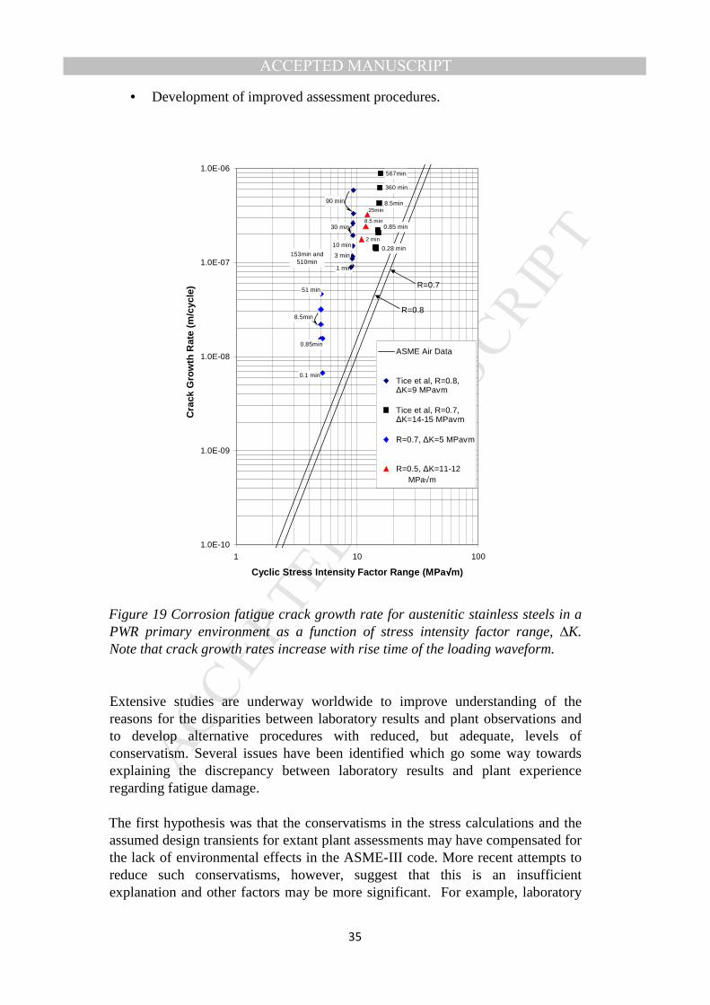
MANUSCRIP

T

ACCEPTED

ACCEPTED MANUSCRIPT

35

• Development of improved assessment procedures.

Figure 19 Corrosion fatigue crack growth rate for austenitic stainless steels in a PWR primary environment as a function of stress intensity factor range, ∆K. Note that crack growth rates increase with rise time of the loading waveform. Extensive studies are underway worldwide to improve understanding of the reasons for the disparities between laboratory results and plant observations and to develop alternative procedures with reduced, but adequate, levels of conservatism. Several issues have been identified which go some way towards explaining the discrepancy between laboratory results and plant experience regarding fatigue damage. The first hypothesis was that the conservatisms in the stress calculations and the assumed design transients for extant plant assessments may have compensated for the lack of environmental effects in the ASME-III code. More recent attempts to reduce such conservatisms, however, suggest that this is an insufficient explanation and other factors may be more significant. For example, laboratory

10 min

90 min

30 min

3 min

1 min

567min

360 min

8.5min

0.85 min

0.28 min

0.85min

8.5min

51 min

153min and 510min

0.1 min

25min

8.5 min

2 min

1.0E-10

1.0E-09

1.0E-08

1.0E-07

1.0E-06

1 10 100

Cyclic Stress Intensity Factor Range (MPa√√√√m)

Cra

ck G

row

th R

ate

(m/c

ycle

)

ASME Air Data

Tice et al, R=0.8,∆K=9 MPavm

Tice et al, R=0.7,∆K=14-15 MPavm

R=0.7, ∆K=5 MPavm

R=0.5, ∆K=11-12MPa?m

R=0.7

R=0.8

MPa√m

�

����

�

�

MANUSCRIP

T

ACCEPTED

ACCEPTED MANUSCRIPT

36

fatigue life (S-N) tests are usually performed on smooth membrane-stressed tensile specimens under strain control using simple triangular waveforms, usually at R=-1, whereas plant transient waveforms are much more complex and strain gradients exist through-wall. Similarly, crack growth tests use triangular, sawtooth or sine wave loading waveforms which are not representative of the complex loading waveforms produced by plant transients. One difficulty in applying the procedures is the need to quantify the rate of change during the complex plant transients, since Fen is dependent on applied strain rate in S-N tests (Fig. 18) and crack growth rate in environment is a function of transient rise time (Fig. 19). Le Duff et al [65] have performed S-N testing with a complex transient simulating a double thermal shock transient for a PWR safety injection system (transient Type A in Fig. 20), as well as using variants of this waveform with the slow and fast portions relocated (Types B, C and D). For the four different transients the experimental Fen values were between 1.7 and 3.7 compared to a value of ~6 predicted by the NUREG/CR-6909 equations. The differences were attributed to the fact that the effect of the environment was greatest when the slow strain rate portion occurred under tensile mean load, whereas the NUREG equations assume a constant environmental effect for the whole transient. Platts et al.[66] have reported somewhat similar effects in crack growth tests (at positive R) in which for two-stage transients (Fig. 20), the environmental enhancement was greatest when the slow rise portion was in the upper ∆K portion of the transient. These observations form the basis of the recently developed weighted K-rate model of Emslie et al [67] which provides a good fit to the experimental data for a range of different waveforms.

Figure 20 Representative loading signal for a thermal transient (Type A) together with modified versions with different parts of the waveform interchanged [64]

MANUSCRIP

T

ACCEPTED

ACCEPTED MANUSCRIPT

37

Another significant difference from most laboratory tests is that many plant tests involve simultaneous variations in both stress and temperature whilst most laboratory tests are isothermal. Since the environmental effect on both fatigue life and crack growth increases with temperature, and the stress and temperature cycles for thermal transients, such as transient A in Figure 20, are typically fairly close to out-of-phase, it might be expected that the environmental enhancement would be reduced for thermal transients. Tests have been carried out using simplified thermal cycling by Seifert et al. for S-N testing [68] and by Platts et al. for crack growth [66], with the observations suggesting that the relevant temperature for predicting the environmental enhancement is best approximated by the temperature at which the load cycle is at its tensile maximum. Other studies are investigating the extent to which the transference factors used to develop the air design curve from the mean air curve in ASME III and NUREG/CR-6909 (12 on cycles or 2 on stress for austenitic steel, whichever is greater) may be over-conservative, especially when multiplied by the Fen factor from NUREG/CR-6909. These transference factors are intended to account for the effects of material variability, data scatter, size effects, surface finish and loading history and are based on observations in an air environment. Métais et al. [64] have argued that the factor of 2 on strain amplitude (or stress), which is applicable in air at relatively numbers of cycles, is excessive for materials relevant to French plant. This was demonstrated using several statistical analysis methods [64]. This approach results in an air curve very similar to the old (pre-2008) ASME XI air curve which was in use for many years before it was modified in line with that in NUREG/CR-6909. Regarding the effect of surface finish, both Le Duff et al. [65] and Platts et al. [66] report smaller differences between fatigue lives for ground and polished specimens in PWR water compared to air, despite the ground surfaces being very different in the two studies. This implies that some of the environmental effects are in effect covered by the transference factor of 12 on cycles and so a lower Fen value than that in NUREG/CR-6909 may be appropriate.

To take account of the above observations that plant-relevant waveforms tend to produce lower environmental enhancement than triangular loading and that surface finish effects are lower in water than in air, EDF introduced a new method for accounting for environmental effects on fatigue which eliminates excessive conservatism [70]. This uses a so-called Fen-integrated which can be used to reduce the value of Fen calculated using the NUREG/CR-6909 Rev. 1 equations. The value of Fen-integrated is taken as 5 for thermal shock transients and 3 for other transients. This approach has recently been accepted as an amendment to the RCC-M design code in France and will be integrated to the code as a “Rule in Probation Phase” (similar to a Code Case in ASME). Finally, it should be noted that several alternative assessment procedures are currently being evaluated by the ASME Section III Working Group on

MANUSCRIP

T

ACCEPTED

ACCEPTED MANUSCRIPT

38

Environmental Fatigue Evaluation Methods. The aim of this group is to evaluate recognised and alternative methods of assessing cyclic life of Class 1 components that are subject to a wetted environment. The life assessment approaches being considered include traditional fatigue usage evaluations, crack growth evaluation methods and other approaches to provide appropriate design margins when a usage factor or an equivalent criterion is determined. Approaches which have been or are being considered include: • Exclusion clauses for cyclic analysis in a water environment; • The use of strain rate dependent water-adjusted fatigue curves. These avoid the unsubstantiated assumption inherent in the Fen approach that the environmental effect is independent of strain rate; • Use of a correction factor to allow for through-thickness strain gradient effects which exist for many thermal plant transients; • The option of a flaw defect approach based on a postulated defect at start of life, in the event that a cumulative usage factor greater than one is calculated when incorporating environmental effects using the standard S-N fatigue design approach; • Development of a Total Life Prediction methodology which accounts for possibly different environmental effects on crack nucleation, microstructurally short, mechanically short and long crack growth, Figure 21. This resembles the UK R5 Code used for high temperature fatigue and creep applications and is being considered in conjunction with the development of a consequence based design factor.

Figure 21 Total Life Prediction approach based on modelling of the different stages

of defect development, from crack nucleation to through-wall leakage

F Ellyin, “Fatigue Damage, Crack Growth and Life Prediction”,1996, Chapman & Hall K Hussain, “Short

Fatigue Crack Behaviour and Analytical Models: A Review”,, Engineering Fracture Mechanics, 58, p.327,1997

M E Fine and Y-W Chung, “Fatigue Failure in Metals”, in ASM Handbook; Volume 19; Fatigue and Fracture”, 1996

MANUSCRIP

T

ACCEPTED

ACCEPTED MANUSCRIPT

39

4.3 Application of a Cellular Automaton and Finite Element (CAFE) model to predict Corrosion Fatigue Damage ( Prof R. Akid)

A promising approach to model the progression of corrosion is via cellular automata modelling. Cellular automata (CA) originally proposed by von Neumann [71], adopts discrete dynamical systems, whilst retaining many properties of continuous dynamical systems. This property makes them a powerful tool for modelling physical, chemical, and biological systems. For example, CAs have recently been exploited to model the progression of corrosion [72-75]. A probabilistic approach is chosen because it enables a convenient simulation of the complex interactions between the chemical reactions in the electrolyte domain and the propagation of the corrosion path in the metal domain. As we are dealing with a mesoscopic description, cells are not to be directly associated with the individual atoms, anions or cations, but to some limit-resolution scale below which we consider the system as unstructured, atomic size effects are thus not accounted for. There are two major stages involved in corrosion fatigue (CF), namely, time dependent corrosion (pitting) and mechanical cycles dependent (fatigue). This need to model both time and mechanics dependent components, significantly limits the use of existing ’pitting’ corrosion fatigue models [76], hence the concept of Cellular Automaton Finite Element (CAFE) modelling has been introduced in an attempt to overcome these limitations. In a CA, the evolution of the state of each cell in the modelling space is determined by the current state of a cell at a discrete time step and that of its neighbourhood cells. All cells have access to the same set of states at any time and can assume only a finite number of states. Based on local transformation rules, which apply to all the cells in the automaton, all cells are updated synchronously. A typical CA mesh is illustrated in Fig. 22a, showing the different types of site involved in the process, which include: • M - metal site in solid state • H - proton site • D - passive film • R - metal site • W - water site • P1- Iron (II) Hydroxide • P2 - Iron (III) Hydroxide In the corrosion process, each cell can assume N possible occupation states (as above),

MANUSCRIP

T

ACCEPTED

ACCEPTED MANUSCRIPT

40

The forward reaction for oxidation of Fe to Fe2+ takes place with a corrosion probability P_corr when at least one acidic site H is in the neighbourhood of a metal site M; the M site will be replaced by a R species. When at least one acidic site H is in the neighbourhood of reactive metal site R, oxidation of Fe2+ to Fe3+ takes place with oxidation probability P_ox; the R site will be replaced by a D species. When at least two of the neighbours of a reactive metal R are neutral sites W, hydrolysis of Fe2+ to Fe(OH)2 takes place with hydrolysis probability P_Hyd1; the R and two W sites are replaced with P1 and two H species respectively. The final reaction involves the hydrolysis of Fe3+ to Fe(OH)3, when at least three neighbours of a D site are neutral sites W. The reaction will take place with hydrolysis probability P_Hyd2 and the D and three W sites will be replaced by P2 and three H species respectively. The CAFE model for the development of stress-assisted pitting in a pipeline steel exposed to a chloride environment has been described in [77]. A typical CA mesh and CAFE output contour plot are shown in Figure 22b below.

(a)

(b)

Figure 22 (a) Typical CA mesh used to represent corrosion in an aqueous environment; (b) typical distribution of equivalent stress around a growing pit (Stress range= 200 MPa, [A – time: 5400 s, maximum pit depth: 126 µm, aspect ratio: 0.47],

MANUSCRIP

T

ACCEPTED

ACCEPTED MANUSCRIPT

41

Here W represents neutral water; H acidic protons; M unreacted metal; R reaction species Fe2+; D reaction species Fe3+; P1 reaction product Fe(OH)2 and P2 reaction product Fe(OH)3. A comparison of the results from pitting experiments with the CA model is given in Figure 23.

Figure 23 Simulation results of maximum pit depth as a function of time, compared to experimental data obtained from pitting tests. Pipeline steel X65, 3.5% NaCl, room temperature, naturally aerated. The role of stress on pit current is introduced via the Gutman equation which relates the anodic current resulting from deformation to the strain at the onset of strain hardening [78]. Critical strain values for the transition between pitting and cracking can be based upon digital image correlation measurements. Strain values at the mouth of a pit have been measured as a function of fatigue cycles, until crack initiation occurred. The strain value at initiation is then taken as the strain for the pit-crack transition.

5 Summary of discussions and conclusions

The workshop provided a platform to discuss knowledge gaps in FFS assessment procedures and life estimation methodologies. Significant progress has been made towards characterizing the role and effect of the different failure mechanisms (fracture, fatigue, creep and/or corrosion, etc.) and their interaction in the structural integrity of engineering materials since the early 20th century. In addition, effort has been made both from academic and industrial players to improve our understanding of the effect of low/high temperatures and/or

MANUSCRIP

T

ACCEPTED

ACCEPTED MANUSCRIPT

42

aggressive environments and how to include their effect in FFS assessment procedures.

By linking the different length scales at which the failure mechanisms evolve, the materials science research community has contributed significantly to reduce the current knowledge gaps and to lead to better understanding of the dependence on local mechanical driving force, local material properties and environment.

In practice, however, simplified assessment methods are required and are usually the first option by the engineering community, as this represents a less cost and time intensive option. Unfortunately, as plants age and get closer to the design life, simplified assessment routes, providing large reserve factors, are unacceptable. During the workshop, the need to make the use of advanced methods more straightforward and to increase their validation, in order to encourage their use in practical plant assessments and their acceptance by regulatory bodies, was stressed. This is an area in which effort is currently focused, to establish more advanced damage tolerance arguments. For example, current numerical modelling capabilities allow stress and strain states within structures and components to be assessed more accurately. The application of constraint-based approaches, ductile/brittle fracture initiation and propagation models and strain-based procedures are now more common and of wide availability. Arguments based on defects due to manufacturing processes, the use of more advanced methods for assessing limit loads and the characterisation of the effect of warm pre-stressing, among others, have been discussed and should allow improvement of current assessment FFS assessment capabilities

It is undeniable that further action is needed to narrow the ‘knowledge gaps’ addressed in the workshop and others gaps not addressed. With this in mind and due to the necessity of most industries to introduce new materials safely or to operate under more challenging conditions (higher pressures, higher temperatures or/and more aggressive environments), adequate (reliable, conservative, accurate, etc.) fitness-for-service assessment approaches will be required and other ‘knowledge gaps’ will undoubtedly arise. A best practice approach of improving the capabilities of each of the standards by incorporating methodologies and recommendations currently available in other procedures should be considered.

Acknowledgments

The authors would like to express their appreciation to the University of Manchester for providing funding (EPS Strategic Fund AA13298) and organizational support for this workshop. Prof R.A. Ainsworth and Dr N.O Larrosa further extend their thanks to the invited speakers for their participation and contribution.

MANUSCRIP

T

ACCEPTED

ACCEPTED MANUSCRIPT

43

REFERENCES REFERENCES [1] R5 Issue 3: Assessment procedure for the high temperature response of

structures, EDF Energy, Gloucester, UK, Revision 002, 2014.

[2] R6 Revision 4, Assessment of the integrity of structures containing defects, EDF Energy, Gloucester, UK, Amendment 11, 2015.

[3] API579-1/ASME FFS-1, Fitness-for-service, American Petroleum Institute/American Society of Mechanical Engineers, Washington DC, USA, 2016.

[4] BS7910:2013+A1:2015, Guide to methods for assessing the acceptability of flaws in metallic structures, British Standards Institution, London, UK, Amendment 1 Corrigendum 2, 2016.

[5] Dong, P., Song, S., Zhang, J., Kim, M.H. On residual stress prescriptions for fitness for service assessment of pipe girth welds. Int J Pres Ves Piping; 123: 19-29, 2014.

[6] Hadley I. Progress towards the Revision of BS 7910. ASME Pres Ves Piping Conference , PVP2011-57307, 2011.

[7] Ainsworth R.A. and O'Dowd N.P. Constraint in the failure assessment diagram approach for fracture assessment. J Pres Ves Tech, Trans ASME, 117 (3), 260-267, 1995.

[8] Gintalas M. and Ainsworth, R.A. Constraint based assessments of large-scale cracked straight pipes and elbows. ASME Pres Ves Piping Conference, PVP2015-45948, 2015.

[9] Ainsworth R.A., Gintalas M., Sahu M.K., Chattopadhyay J. and Dutta B.K. Application of failure assessment diagram methods to cracked straight pipes and elbows. Int J Pres Ves Piping, 148, pp. 26-35, 2016.

[10] Larrosa N.O. and Ainsworth R.A. A transferability approach for reducing excessive conservatism in fracture assessments. Engng Fract Mech, Article in Press, 2016.

[11] Han J-J., Larrosa N.O., Kim Y-J. and Ainsworth R.A. Blunt defect assessment in the framework of the failure assessment diagram. Int J Pres Ves Piping;146: 39–54, 2016.

[12] Kim J., Larrosa N.O., Horn A.J., Kim Y-J. and Ainsworth, R.A. Notch bluntness effects on fracture toughness of a modified S690 steel at 150°C Engng Fract Mech. Under Review, 2017.

[13] Ainsworth R.A. An assessment of the effects of prestrain on upper shelf fracture toughness, J Strain Anal Eng 21, 219-223, 1986.

[14] Ainsworth R.A., Larrosa N.O., Kim J-S., Jeon, J-Y. and Kim J-Y. Prestrain effects on ductile tearing resistance, EDF Energy Report E/REP/BBGB/0198/GEN/16, 2016.

MANUSCRIP

T

ACCEPTED

ACCEPTED MANUSCRIPT

44

[15] API 579-2/ASME FFS-2 2009 Fitness-for-service Example problem manual, API, 2009.

[16] Larrosa N.O., Ainsworth R.A. Comparisons of the solutions of common FFS standard procedures to benchmark problems. Int J Press Vessels Pip, 139-140, pp. 36-46, 2016.

[17] Song S., Dong P., and Zhang P., A Full-Field Residual Stress Estimation Scheme for Fitness-For-Service Assessment of Pipe Girth Welds: Part I: Identification of Key Parameters, International Journal of Pressure Vessels and Piping, 2015; 126- 127:58-70

[18] Song S., Dong P., and Pei X., A Full-Field Residual Stress Estimation Scheme for Fitness-For-Service Assessment of Pipe Girth Welds: Part II: A Full-Field Estimation Scheme, Int J Press Vessels Pip, 128:8-17, 2015

[19] Song S, Dong P, A residual stress profile estimation method for fitness-for-service assessment of pipe seam welds: Part I – Weld region, , Int J Press Vessels Pip, 146:74-86, 2016.

[20] Song S, Dong P, A residual stress profile estimation method for fitness-for-service assessment of pipe seam welds: Part II – Outside of weld region, Int J Press Vessels Pip, 146:65-73, 2016

[21] RSE-M: In-service inspection rules for mechanical components of PWR nuclear islands, 2010 edition, AFCEN, Paris, France, including addenda to No.4, 2015.

[22] Kǫcak M., Webster S., Janosch J.J. and Ainsworth R.A. (editors), Procedure (Volume 1), ISBN 978-3-940923-00-4, Annex (Volume 2), ISBN 978-3-940923-01-1, FITNET Fitness-for-Service (FFS), Revision MK8, GKSS Research Centre, Geesthacht, Germany, 2008.

[23] Budden P.J. and Sharples J.K., The R6 defect assessment procedure: status and key recent developments, Trans. 24th Structural Mechanics in Reactor Technology (SMiRT-24), Manchester, UK, August 2015, IASMiRT.

[24] Budden P.J., Developments in UK defect assessment methods, Proc. 13th Engineering Structural Integrity Assessment (ESIA 13), Manchester, May 2015, EMAS, 2015.

[25] Ainsworth R.A., The treatment of elastic follow-up within R6 for combined primary and secondary stresses, Report E/REP/BBGB/0183/GEN/16, EDF Energy, Gloucester, UK, 2016.

[26] DNV-OS-F101, Submarine pipeline systems, DNV-GL, 2013.

[27] Likens D., Formby C.L. and Ainsworth R.A. A strain-based approach to fracture assessment – example applications, Proc Conf Engng Structural Assessment, Cambridge, EMAS, 2000.

[28] Budden P.J. and Ainsworth R.A. The shape of a strain-based failure assessment diagram, Int J Pres Ves Piping 89, 59-66, 2012.

[29] Budden P.J. and Smith M.C., Numerical validation of a strain-based failure assessment diagram approach to fracture, Paper PVP2009-77377, Proc ASME PVP Conference, Prague, 2009.

MANUSCRIP

T

ACCEPTED

ACCEPTED MANUSCRIPT

45

[30] Ainsworth R.A., Budden P.J., Oh C-Y. and Kim Y-J. The treatment of secondary strains within a strain-based failure assessment diagram, Int J Pres Ves Piping 104, 14-20, 2013.

[31] Lei Y. and Ainsworth R.A., Failure assessment diagrams for cracks in welds with mismatched mechanical properties, Proceedings ASME PVP Conference, Montreal, Canada, ASME PVP Vol 324 Number 2, pp.65-73, 1996.

[32] Lei Y. and Ainsworth R.A., A J estimation method for cracks in welds with mismatched mechanical properties, Int J Pres Ves Piping 70, 237-246, 1997.

[33] Bouchard P.J., Budden P.J. and Withers P.J., Fourier basis for the engineering assessment of cracks in residual stress fields, Engng Fract Mech 91, 37-50, 2012.

[34] Meek C. and Ainsworth R.A., The effects of load biaxiality and plate length on the limit load of a centre-cracked plate, Engng Fract Mech 147, 306-317, 2015.

[35] Lei Y. and Budden P.J., Global limit load solutions for plates with surface cracks under biaxial forces and cross-thickness bending, Int J Pres Ves Pip 132-133, 10-26, 2015.

[36] Chell G.G. and Curry D.A. Mechanics and mechanisms of cleavage fracture, Section 8 ‘Generalised loading’ in ‘Developments in fracture mechanics’, G G Chell (editor), Applied Science, London, 11-177, 1981.

[37] Wallin K., Master Curve implementation of the warm pre-stress effect, Engng Fract Mech 70, 2587-2602, 2003.

[38] Moinereau D., Landron C., Chapuliot S. and Marie S., Validation of ACE analytical criterion in RPV integrity assessment, Proc ASME PVP Conference, Paper PVP2015-45103, Boston, USA, 2015.

[39] Van Gelderen D.G.A, Booker J.D. and Smith D.J., Evaluating the conditions when warm pre-stressing does not produce a benefit in apparent toughness, Materials Today, 2014.

[40] Van Gelderen D.G.A, Rosahl K, Booker J.D. and Smith D.J., Monte Carlo simulations of the effects of warm pre-stress on the scatter in fracture toughness, Engng Frac Mech 134, 124-147, 2015.

[41] Mehmanparast A.N., Davies C.M., Dean D.W. and Nikbin K.M. The influence of cold pre-compression on high temperature deformation and fracture behaviour of 316H stainless steel. International Conference on Engineering Structural Integrity Assessment 24th.

[42] Mehmanparast A.N., Davies C.M., Dean D.W. and Nikbin K.M. The Influence of Inelastic Damage on Tensile Deformation and Creep Crack Growth Behaviour of Type 316H Stainless Steel ASME 2013 Pressure Vessels and Piping Conference, V06AT06A044-V06AT06A044

[43] Mehmanparast A.N., Davies C.M., Nikbin K.M and Webster G.A. Creep Crack Growth Predictions in 316H Steel Over a Wide Range of Stresses and Temperatures. ASME 2014 Pressure Vessels and Piping Conference, V06AT06A041-V06AT06A041

MANUSCRIP

T

ACCEPTED

ACCEPTED MANUSCRIPT

46

[44] Mehmanparast A.N., Davies C.M., Webster G.A. and Nikbin K.M. Creep crack growth rate predictions in 316H steel using stress dependent creep ductility. Materials at High Temperatures 31 (1), 84-94.

[45] Mehmanparast A.N., Davies C.M., Dean D.W. and Nikbin K.M. The influence of pre-compression on the creep deformation and failure behaviour of Type 316H stainless steel. Engineering Fracture Mechanics 110, 52-67

[46] Mehmanparast A.N., Davies C.M., Dean D.W. and Nikbin K.M. Material pre-conditioning effects on the creep behaviour of 316H stainless steel. International journal of pressure vessels and piping 108, 88-93.

[47] Tarnowski K.M., Davies C.M., Dean D.W. and Nikbin, K.M. Measuring Creep Crack Initiation and Growth in Ductile Materials Using the Potential Drop Method. In preparation.

[48] Tarnowski K.M., Davies C.M., Dean D.W. and Nikbin K.M. The Influence of Plasticity on Crack Length Measurements Using the Potential Drop Technique. Evaluation of Existing and New Sensor Technologies for Fatigue, Fracture and Mechanical Testing. Editors: Jidong Kang, David Jablonski, David Dudzinski.

[49] Tarnowski K.M., Davies C.M., Nikbin K.M and Dean D.W. The Influence of Creep Strain on Crack Length Measurements Using the Potential Drop. ASME 2015 Pressure Vessels and Piping Conference, V06AT06A044-V06AT06A044

[50] Tarnowski K.M., Davies C.M., Nikbin K.M and Dean D.W. The influence of strain on crack length measurements using the potential drop technique. 16th International Conference on Experimental Mechanics, 7th to 11th July 2014, University of Cambridge, UK.

[51] Turnbull A., Zhou S. and Lukaszewicz M. An approach to measurement of environmentally assisted small crack growth, Corrosion 2013, NACE International, Paper no, C-2013-0002122.

[52] EI Haddad M.H., Smith K.N. and Topper T.H., Fatigue crack propagation of short cracks, ASME Journal of Engineering Materials and Technology, 101, (1979) 42-46.

[53] Zhou S. and Turnbull A., Influence of pitting on the fatigue life of turbine blade steel, Fatigue Fract. Engng Mater. Struct., 22 (1999) 1083-1093.

[54] Turnbull A. and Zhou S., Electrochemical short crack effects in environment assisted cracking of steam turbine blade steel, Corros. Sci., 58 (2012) 33-40.

[55] Zhou S. and Lukaszewicz M. and Turnbull A., Small and short crack growth and the solution-conductivity dependent electrochemical crack size effect, Corros. Sci., 97 (2015) 25-37.

[56] Chopra O.K. and Shack W.J., Effects of LWR Coolant Environments on Fatigue Design Curves of Carbon and Low-Alloy Steels, NUREG/CR-6583, February 1998

[57] Chopra O.K., Effect of LWR Coolant Environments on Fatigue Design Curves of Austenitic Stainless Steels, NUREG/CR-5704, April 1999

MANUSCRIP

T

ACCEPTED

ACCEPTED MANUSCRIPT

47

[58] Ford F.P., Quantitative Prediction of Environmentally Assisted Cracking, Corrosion 52, pp375-395, 1996

[59] Mills W.J., Accelerated and Retarded Corrosion Fatigue Crack Growth Rates for 304 Stainless Steel in an Elevated Temperate Aqueous Environment, Proc. 16th Int. Conf. on Environmental Degradation in Nuclear Power Systems – Water Reactors, Asheville, NC, USA, August 2013

[60] Chopra O K and Shack W J, Effect of LWR Coolant Environments on the Fatigue Life of Reactor Materials – Final Report, NUREG/CR-6909, February 2007

[61] Chopra O.K. and Stevens G.L., Effect of LWR Coolant Environments on the Fatigue Life of Reactor Materials – Draft Report for Comment, NUREG/CR-6909 Rev. 1, March 2014

[62] Tice D.R., Platts N., Rigby K. and Stairmand J.W., Effect of Temperature and Flow Rate on the Corrosion Fatigue Crack Growth of Austenitic Stainless Steel in a PWR Primary Coolant Environment, Proc. 13th Int. Conf. on Environmental Degradation in Nuclear Power Systems, Whistler, British Columbia, Canada, August 2007

[63] Tice D.R., Green D. and Toft A., Environmentally Assisted Fatigue Gap Analysis and Roadmap for Future Research – Gap Analysis Report, December 2011, EPRI, Palo Alto, CA, USA, 1023012

[64] Tice D.R., Green D. and Toft A. Environmentally Assisted Fatigue Gap Analysis and Roadmap for Future Research: Roadmap, December 2012, EPRI, Palo Alto, CA, USA, 1026724

[65] Le Duff J.A., Lefrançois A, Vernot J.P. and Bossu D., Effect of Loading Signal and of Surface Finish on the Low Cycle Fatigue Behavior of 304L Stainless Steel in PWR Environment, Proc. ASME Pressure Vessel and Piping Conference, Bellevue. WA, USA, July 2010; PVP2010-26027

[66] Platts N, Tice D R, Stairmand J W and Swan D.I., The Effect of Complex Loading Waveforms and Non-Isothermal Conditions on Environmentally Enhanced Fatigue Crack Growth of Austenitic Stainless Steel. Proc. 16th Int. Conf. on Environmental Degradation in Nuclear Power Systems – Water Reactors, Asheville, NC, USA, August 2013

[67] Emslie J., Gill C. and Wright K., Assessment Method to Account for the Rise Time of Complex Waveforms in Stainless Steel Environmental Fatigue Crack Growth Calculations , Proceedings of the ASME 2016 Pressure Vessels and Piping Conference, July 17-21, 2016, Vancouver, British Columbia, Canada, ASME PVP2016-63497

[68] Seifert H.P. and Ritter S., Thermo-Mechanical and Isothermal Low-Cycle Fatigue Behavior of Type 316L Stainless Steel in High-Temperature Water and Air”, Corrosion 69, pp1012-023, 2013

[69] Métais T., Courtin S., Genette P., De Baglion L., Gourdin C. and Le Roux J. Overview of French Proposal of Updated Austenitic SS Fatigue Curves and

MANUSCRIP

T

ACCEPTED

ACCEPTED MANUSCRIPT

48

of a Methodology to Account for EAF. Proc. ASME Pressure Vessel and Piping Conference, Boston, MS, USA, July 2015; PVP2015-45158

[70] Stairmand J.W., Platts N., Tice D.R., Mottershead K., Zhang W, Meldrum J and McLennan A. Effect of Surface Condition on the Fatigue Life of Austenitic Stainless Steels in High Temperature Water Environments. Proc. ASME Pressure Vessel and Piping Conference, Boston, MA, USA, July 2015; PVP2015-45029

[71] von Neumann J, Burks A.W.. Theory of Self-reproducing Automata. University of Illinois Press, Urbana (1966)

[72] Pidaparti R.M. , Palakal M.J., Fang L. . Cellular automata approach to aircraft corrosion growth. Int. J. Artif. Intell. Tools, 14 (2005), pp. 361-369

[73] Meakin P., Jøssang T., Feder J.. Simple passivation and depassivation model for pitting corrosion. Phys. Rev. E, 48 (1993), pp. 2906-2916

[74] Reigada R., Sagus F., Costa JM. A Monte Carlo simulation of localised corrosion. J. Chem. Phys., 101 (1994), pp. 2329-2337

[75] Malki B, Baroucx B.. Computer simulation of corrosion pit growth. Corros. Sci., 47 (2005), pp. 171-182

[76] Larrosa NO., Akid R., Ainsworth RA. Corrosion-fatigue: a review of damage tolerance models, Int Mater Rev, 2017, In Press, DOI: 10.1080/09506608.2017.1375644

[77] Fatoba O., Leiva-Garcia R., Akid R., Lishchuk S.V., Larrosa N.O. Modelling stress-assisted pitting corrosion using a Cellular Automaton Finite Element Approach. Submitted to Corrosion Science, 2017.

[78] Gutman E.M. Mechanochemistry of Materials. Cambridge: Cambridge International Science Publishing, 1998.

MANUSCRIP

T

ACCEPTED

ACCEPTED MANUSCRIPT

Highlights:

Knowledge gaps in defect assessment by using fitness-for-service procedures are highlighted.

Issues related to creep, fracture, corrosion fatigue, environmentally assisted fatigue, Welding Residual Stresses are covered.

Some recent efforts focused in addressing these knowledge gaps are described.