An Adjoint Sensitivity Analysis and 4D-Var Data

Assimilation Study of Texas Air Quality

Lin Zhang, E.M. Constantinescu, A. Sandu Virginia Polytechnic Institute and State University

Y. Tang, T. Chai, G.R. Carmichael University of Iowa

D. Byun University of Houston

E. Olaguer Houston Advanced Research Center

ABSTRACT: In this paper we discuss the theory of adjoint sensitivity analysis and the method of 4D-Var data assimilation in the context of the Sulfur Transport Eulerian Model (STEM). The STEM atmospheric Chemical Transport Model (CTM) is used to perform adjoint sensitivity analysis and data assimilation over the State of Texas.

We first demonstrate the use of adjoint sensitivity analysis for a receptor located at ground level in the Dallas Fort Worth (DFW) area. Simulations are carried out for three 36-hour intervals in July 2004. One set of simulations focuses on a passive tracer, and illustrates the influence of meteorological conditions. The other results show the areas of influence associated with DFW ground level ozone, i.e. the areas where changes in precursors (O3, NO2, and HCHO) have the maximum impact on DFW ozone. Next, we employ data assimilation to optimize initial conditions of chemical fields and ground level emissions. We optimize the initial conditions for two episodes on July 1 and on July 16, 2004. Data assimilation makes use of AirNow ground level observations (for both episodes) and SCHIAMACHY NO2 and HCHO observations from ENVISAT (for the July 16 episode). The re-analyzed chemical fields show considerable improved agreement with AirNow observations for non-initial conditions.

We also perform inverse modeling of ground level emissions using data assimilation under an additional smoothness constraint. The results indicate higher NO2 emission levels than in the current emission inventory in the DFW area, and lower emission levels in eastern Texas. The formaldehyde emissions are found to be larger than reported in a localized area near the Gulf Coast, and about at the reported level elsewhere. While the results obtained with the current state of the art tools can help guide tuning of emission inventories, better constraints on the inverse problem are needed to obtain more rigorous quantitative estimates. Keywords: Chemical Transport Model, Adjoint Sensitivity Analysis, Data Assimilation

1 INTRODUCTION:

Sensitivity analysis is a methodology that computes the change in the solution of a model with respect to the perturbation of model variables such as initial conditions, parameters, etc. Cacuci et al. [1,2] presented the mathematical foundations of sensitivity analysis for nonlinear dynamical systems and various classes of response functionals. Because it is a powerful tool with diverse applications, sensitivity analysis is receiving increased attention in the field of air quality modeling.

Traditional direct sensitivity analysis calculates the rate of change of model solutions with respect to perturbation of input parameters one at a time. The Decoupled Direct Method (DDM) [3] uses this technique to obtain sensitivities of all state variables with respect to a few parameters. However, DDM is infeasible for systems with a large number of parameters. Adjoint sensitivity analysis, on the other hand, has the advantage of efficiently calculating the derivatives of a functional with respect to a large number of parameters. Sandu et al. [4] discussed the mathematical foundations of the adjoint sensitivity method as applied to air quality models, and present computational tools for performing three-dimensional adjoint sensitivity analysis. Henze and Seinfeld [5] illustrated the application of adjoint sensitivity analysis in the GEOS-Chem global model. In this paper, we utilize the adjoint approach in the STEM model to investigate the maximum area of influence within the atmosphere on ozone concentrations in the DFW area.

Data assimilation is the process by which measurements are used to constrain model predictions. The information from measurements can be used to obtain better initial and boundary conditions, enhanced emission estimates, etc. Because of this, data assimilation is an essential component in weather and climate forecasting.

4D-Var data assimilation allows the optimal combination of three sources of information: a priori (“background”) estimate of the state of the atmosphere; knowledge of the interrelationships among the chemical fields that are simulated by the CTM; and observations of some of the state variables. The optimal state is obtained by minimizing an objective function to provide the best fit to all observational data.

The implementation of the 4D-Var data assimilation technique in large-scale atmospheric models relies on adjoint modeling to provide the gradient of the objective function. Mathematical foundations of the adjoint sensitivity technique for nonlinear dynamical systems are presented by Cacuci [1,2] and Marchuk et al. [6,7]. Early applications of 4D-Var to chemical data assimilation were proposed by Fisher and Lary [8]. Both 4D-Var and the Kalman filter method were implemented in a model by Khattatov et al. [9]. Elbern et al. [10] used a tropospheric gas-phase box model to analyze the applicability of 4D-Var to tropospheric chemical data assimilation. In the past few years variational methods have been successfully used in data assimilation for comprehensive three-dimensional atmospheric chemistry models (Elbern and Schmidt [11], Errera and Fonteyn [12]). Wang et al.[13] provide a review of applications of the adjoint methodology and data assimilation to atmospheric chemistry. In [14] Elbern et al. study the skill and limits of 4D-Var techniques in analyzing emission rates of ozone precursors when only ozone observations are available. They also discuss improvements in ozone prediction achieved through the assimilation of observations in [15].

In this paper we summarize simulations of Texas air quality using the STEM chemical transport model and the results of data assimilation for the model initial conditions. Modeling was conducted for the entire state of Texas using two meteorological episodes on July 1 and July 16,

2004. In the first episode, we used only AirNow ground level observations as inputs for data assimilation, whereas in the second, we also used SCHIAMACHY satellite measurements of NO2 and HCHO. The re-analyzed chemical fields show considerable improved agreement with AirNow observations for non-initial conditions (the R2 correlation coefficients increase from about 0.35 to over 0.7). Data assimilation was also used to improve estimates of ground level emissions for different assimilation times. The results of this inverse modeling show consistency with each other and confirm the inversion procedure, though further investigation is needed.

The paper is organized as follows: the second section briefly introduces the STEM chemical transport model. The third section presents the theory of adjoint sensitivity analysis and compares its results to those obtained by direct sensitivity analysis. The fourth section presents the 4D-Var data assimilation technique, as well as optimization results for initial conditions and emissions. Section five presents a summary of conclusions.

2 The STEM Chemical Transport Model The STEM is a regional atmospheric chemical transport model (CTM). Taking emissions, meteorology (wind, temperature, humidity, precipitation etc.) and a set of chemical initial and boundary conditions as input, it simulates the behavior of pollutants in the selected domain. A CTM can be represented as a system of coupled partial differential equations discretized in both time and space:

( ) ( ) FkptyypytMy kkk ,,2,1,,,,, 0011 K=== −− (2.1)

where nky ℜ∈ is the state vector representing the concentration field at time kt , M is a discrete

solution operator of the advection-diffusion-reaction equation, and mp ℜ∈ the vector of model

parameters (e.g., initial conditions, emission rates, etc). Its solution is uniquely determined by the

initial state and the model parameters ),( ptyy = .

STEM-2K3 is a regional chemical transport model developed from STEM-2K1 [16,17] that includes the Statewide Air Pollution Research Center's chemical mechanism (SAPRC-99) gaseous mechanism [18] and an explicit photolysis-rate solver. STEM-2K3 also includes an aerosol thermodynamics module, SCAPE II (Simulating Composition of Atmospheric Particles at Equilibrium) [19,20], for calculating gas-particle equilibrium concentrations among inorganic aerosol ions and their gaseous precursors. Tang et al. [21] described the framework of STEM-2K3 and its performance during the Transport and Chemical Evolution over the Pacific (TRACE-P) experiment and the Asian Pacific Regional Aerosol Characterization Experiment (ACE-Asia). The primary domain for STEM-2K3 covers the U.S. For each domain we ran Fifth-Generation Mesoscale Model (MM5) forecasts initialized by Global Aviation Model (AVN) products to provide the meteorological fields needed by the STEM model. The Model of Ozone and Related Chemical Tracers (MOZART) global forecasts were used to specify lateral boundary conditions for the STEM-2K3 primary domain. STEM was run with a horizontal resolution of 60Km by 60Km, and with 21 vertical levels defined by the Regional Atmospheric Modeling System’s sigma-z coordinate system. The domain

covered the entire State of Texas and parts of the surrounding States, ranging from 92°W to 108°W in longitude and from 28°N to 32°N in latitude. The simulations were for July of 2004, a time period for which much observational data are available for data assimilation. The dynamical time step employed for the simulations was 15 minutes.

3 Sensitivity Analysis Sensitivity analysis is a formal method to assess the rate of change of a model’s solution (2.1) when small perturbations are made to the initial values and/or to the model parameters. The rate of change of the solution with respect to the i-th model parameter (i.e., the sensitivity of the solution with respect to the i-th parameter) is denoted by

.,)()(i

kki

ii p

ySptytS

∂∂

=∂∂

= (3.1)

When the model solution and model parameters have different magnitudes, or different units, it is advantageous to consider scaled sensitivity coefficients

.)(

)()(ˆty

pptytS i

ii ⋅

∂∂

= (3.2)

The scaled sensitivity coefficients are non-dimensional and can be interpreted as the percentage change in the solution when the parameter value is increased by 1%.

3.1 Direct Sensitivity Analysis: A Source-Oriented Approach

The sensitivities of the model solution evolve in time according to the linearized model dynamics:

( ) ( ) .1,,,,,,0

011111 FkpySpyt

pMSpyt

yMS

ii

kk

i

ki

kkki ≤≤

∂∂

=∂∂

+∂∂

= −−−−− (3.3)

Direct sensitivity analysis solves both the model and the sensitivity equation, and advances them forward in time. Note that there are as many sensitivity equations to solve as there are parameters,

mi ≤≤1 . Computational savings are possible by reusing the same linear algebra factorizations in the forward model and in all the sensitivity equations (the direct decoupled method for sensitivity analysis).

To interpret direct sensitivity analysis, consider 0yp = to be the vector of initial

concentrations, and consider a small change ipδ in the concentration of a certain species at the

initial time and at a specific “source” location i (e.g., more NO2 has been released at the initial time at the source location). The changes in the concentration field at later times and at all locations

ii ptSty δδ )()( = , due to the change in the source at the initial time, are obtained at successive

times in the future by solving the sensitivity equation forward in time,

( ) ,0,, 0

0011 Fke

yySSy

yMS i

ii

ki

kki ≤≤=

∂∂

=⋅∂∂

= −− (3.4)

where ie is a vector with all entries equal to zero, except for entry I, which is equal to 1. The

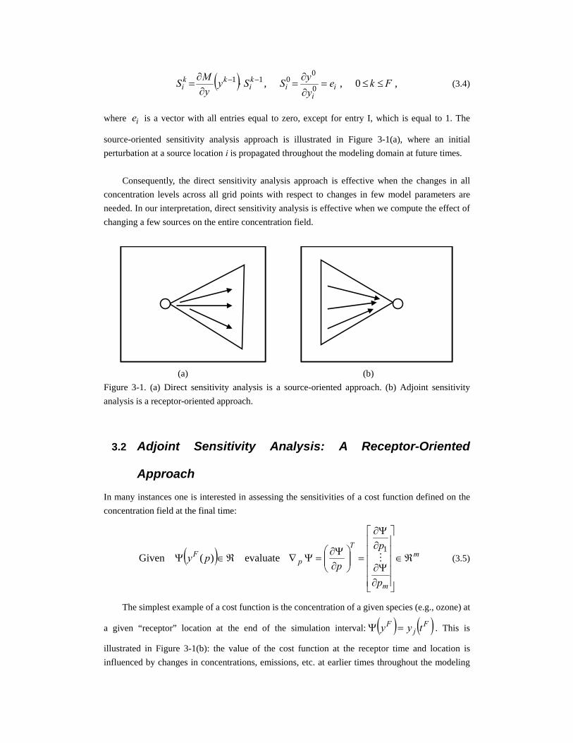
source-oriented sensitivity analysis approach is illustrated in Figure 3-1(a), where an initial perturbation at a source location i is propagated throughout the modeling domain at future times. Consequently, the direct sensitivity analysis approach is effective when the changes in all concentration levels across all grid points with respect to changes in few model parameters are needed. In our interpretation, direct sensitivity analysis is effective when we compute the effect of changing a few sources on the entire concentration field.

00 yy

yy

N

N ∂∂

∂∂

=∂∂ ψψ

00 yy

yy

N

N ∂∂

∂∂

=∂∂ ψψ

00 yy

yy

N

N ∂∂

∂∂

=∂∂ ψψ

(a) (b) Figure 3-1. (a) Direct sensitivity analysis is a source-oriented approach. (b) Adjoint sensitivity analysis is a receptor-oriented approach.

3.2 Adjoint Sensitivity Analysis: A Receptor-Oriented

Approach

In many instances one is interested in assessing the sensitivities of a cost function defined on the concentration field at the final time:

( ) m

m

T

pF

p

p

ppy ℜ∈

⎥⎥⎥⎥⎥

⎦

⎤

⎢⎢⎢⎢⎢

⎣

⎡

∂Ψ∂

∂Ψ∂

=⎟⎟⎠

⎞⎜⎜⎝

⎛∂Ψ∂

=Ψ∇ℜ∈Ψ M1

evaluate)(Given (3.5)

The simplest example of a cost function is the concentration of a given species (e.g., ozone) at

a given “receptor” location at the end of the simulation interval: ( ) ( )Fj

F tyy =Ψ . This is

illustrated in Figure 3-1(b): the value of the cost function at the receptor time and location is influenced by changes in concentrations, emissions, etc. at earlier times throughout the modeling

domain. Using the chain rule, the sensitivity of the cost function with respect to the parameters can be

expressed as:

( ) ( ) FiF

F

i

FS

yy

py

∂Ψ∂

=∂Ψ∂

(3.6)

Consequently, using the direct sensitivity analysis approach, the sensitivity of the concentration at the receptor location can be obtained only after computing the sensitivities of all concentrations at all grid points.

For simplicity, consider again the case where the parameters are the initial conditions 0yp = .

The sensitivity of the cost function with respect to all parameters is given by the chain rule:

( ) ( ) ( )

.1,

,,,

0

111

0

0

1

1

miepy

yty

Myy

py

yy

yy

yy

py

ni

i

nxnkkk

k

iF

F

F

F

i

F

≤≤ℜ∈=∂∂

ℜ∈∂∂

=∂∂

∂∂⋅

∂∂

∂∂

⋅∂Ψ∂

=∂Ψ∂ −−

−− L

(3.7)

Working from right to left for each parameter i=1,…,m the vector ie is multiplied by matrices

),(// 111 −−− ∂∂=∂∂ kkkk ytyMyy for k=1,…,F. Each matrix-vector multiplication corresponds to

solving one step of the sensitivity equations. A more effective computational process is obtained by the transposed chain rule:

( ) ( ) ( ) T

F

FT

F

FTTFF

p yy

yy

yy

pyy ⎟

⎟⎠

⎞⎜⎜⎝

⎛

∂Ψ∂

⋅⎟⎟⎠

⎞⎜⎜⎝

⎛

∂∂

⋅⎟⎟⎠

⎞⎜⎜⎝

⎛

∂∂

=⎟⎟⎠

⎞⎜⎜⎝

⎛

∂Ψ∂

=Ψ∇ −10

1L (3.8)

Working from right to left again the vector Fy∂Ψ∂ / is multiplied successively by matrices

( )Tkk yy 1/ −∂∂ for k = F,…,1. This process needs to be performed only once regardless of the

number of parameters m, and is therefore very efficient. Each matrix-multiplication corresponds to one step of the adjoint model; note that the adjoint steps are taken in reverse order, from F down to

0. Formally if we denote by kλ the adjoint variables and impose the condition that they satisfy the

following adjoint equations:

( ) ( ) ,1,, 111

1 ≥≥⎟⎟⎠

⎞⎜⎜⎝

⎛∂∂

=⎟⎟⎠

⎞⎜⎜⎝

⎛

∂∂

=⎟⎟⎠

⎞⎜⎜⎝

⎛

∂Ψ∂

= −−−

− kFyty

Myy

yy k

Tkkk

T

F

Fk

T

F

FF λλλλ (3.9)

then the adjoint variables are the gradients of the cost function with respect to changes in the state at earlier time:

( ) ( )Fy

T

k

Fk y

yy

kΨ∇=⎟⎟⎠

⎞⎜⎜⎝

⎛

∂Ψ∂

=λ (3.10)

For the general situation the sensitivity of the cost function with respect to model parameters is obtained by a single integration of the adjoint model backwards in time, and the relation:

( ) miytpM

py F

k

kT

kk

i

T

ipi

≤≤⎟⎟⎠

⎞⎜⎜⎝

⎛∂∂

+⎟⎟⎠

⎞⎜⎜⎝

⎛

∂∂

=Ψ∇ ∑=

−− 1,,1

1100

λλ (3.11)

Note that the same adjoint variables are used to obtain the sensitivities with respect to all parameters; a single backward integration of the adjoint model is sufficient. Marchuk [6] presents the computation of adjoint equations for complicated systems.

The adjoint variables (3.11) are also called influence functions. They represent the sensitivity

of the response functional with respect to the variations in the model state at time kt and location

i :

( ) .ki

Fki y

y∂Ψ∂

=λ (3.12)

As in (3.2), it is of interest to consider scaled influence functions, which represent the percentage change in the cost function when the concentration of a certain species at a certain location is changed by 1%,

( )( ).ˆ

F

ki

ki

Fki y

yyy

Ψ⋅

∂Ψ∂

=λ (3.13)

The distributions of the influence functions (adjoint variables) in the three-dimensional computation domain, which are available at any instant, provide the essential information for the sensitivity analysis [4]. For instance, isosurfaces of the ith adjoint variable (x:λi(t,x) = constant) delineate “instantaneous areas of influence”, i.e. locations where perturbations in the concentration of the ith species will produce significant changes in the response function, e.g. the observed PM level at the receptor site and time. Denote time integrals of the adjoint variables over the time period of interest as

∑∑==

==F

k

kF

k

k IorI00

ˆˆ λλ . (3.14)

These are “integrated areas of influence”, i.e. regions where the cumulative effect of concentration changes of the ith species over the interval of interest will affect the target most. In conclusion, we make the following statements.

• Adjoint sensitivity analysis can be used to delineate areas of influence which provide information on the location of major influence factors with respect to a given receptor site and time. This offers a powerful method to characterize source-receptor relationships;

• Areas of influence cannot be computed based solely on inverting meteorological fields, due to the influence of turbulent diffusion and complicated chemical reactions.

3.3 Results

Adjoint sensitivity analysis was performed for a cost function that measures ground level ozone concentration in the DFW receptor area. In order to understand the influence of the meteorological conditions (separately from the chemistry) on the adjoint, the adjoint sensitivities of a passive tracer were also computed. Simulations were carried out for two 36-hour intervals in July 2004; the first interval starts at 9 am July 1st, while the second starts at 9 am July 25th 2004. We also examined the July 16 episode and found that it had a flow pattern somewhat similar to July 25, so the corresponding results are not presented here.

We first consider he scaled adjoint sensitivities of DFW ozone with respect to earlier concentrations of O3, NO2, and HCHO. Specifically, we present the “integrated areas of influence”, i.e. the time integrals of scaled adjoint sensitivities of DFW ozone. The scaled adjoint variables are non-dimensional and can be interpreted as the relative contributions of each perturbation to the observed change in DFW ozone concentrations. The total relative (percent) change in DFW ozone is the sum of the scaled adjoint variable in each grid cell times the relative (percent) perturbation of the precursor concentrations in that grid cell. Since perturbations that appear at any of the earlier times can affect DFW ozone, the adjoint variables are time dependent: the contribution of each grid cell to the DFW ozone changes with the time a perturbation is introduced. To present synthetically all these influences, we “aggregate” the adjoint variables at all times into a single area of influence by performing a time integration. These results are shown next.

For the tracer calculations, the integrated areas of influence for the adjoint sensitivity (without scaling) are shown. These adjoint variables can be interpreted as the relative contributions of the perturbations in each grid cell to ozone concentration in the DFW area. Specifically, the total change in DFW ozone concentration is the sum of the adjoint variable in each grid cell times the perturbation (of ozone or a precursor) in that grid cell.

3.3.1 July 1, 2004

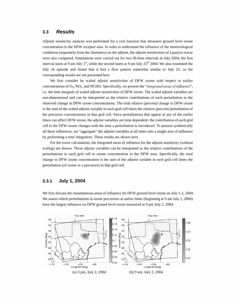
We first discuss the instantaneous areas of influence for DFW ground level ozone on July 1-2, 2004. We assess which perturbations in ozone precursors at earlier times (beginning at 9 am July 1, 2004) have the largest influence on DFW ground level ozone measured at 9 pm July 2, 2004.

(a) 3 pm, July 2, 2004 (b) 9 am, July 2, 2004

(c) 9 pm, July 1, 2004 (d) 9 am, July 1, 2004

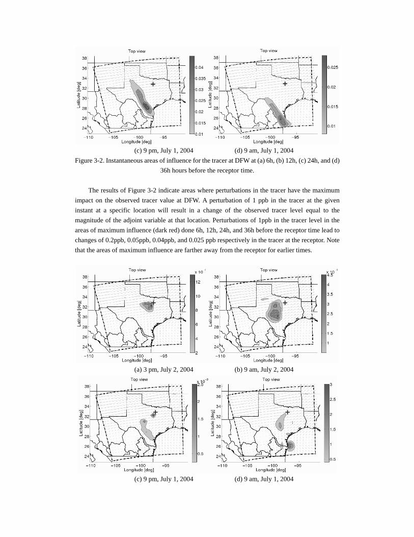
Figure 3-2. Instantaneous areas of influence for the tracer at DFW at (a) 6h, (b) 12h, (c) 24h, and (d) 36h hours before the receptor time.

The results of Figure 3-2 indicate areas where perturbations in the tracer have the maximum

impact on the observed tracer value at DFW. A perturbation of 1 ppb in the tracer at the given instant at a specific location will result in a change of the observed tracer level equal to the magnitude of the adjoint variable at that location. Perturbations of 1ppb in the tracer level in the areas of maximum influence (dark red) done 6h, 12h, 24h, and 36h before the receptor time lead to changes of 0.2ppb, 0.05ppb, 0.04ppb, and 0.025 ppb respectively in the tracer at the receptor. Note that the areas of maximum influence are farther away from the receptor for earlier times.

(a) 3 pm, July 2, 2004 (b) 9 am, July 2, 2004

(c) 9 pm, July 1, 2004 (d) 9 am, July 1, 2004

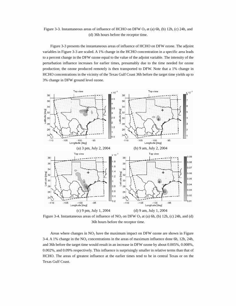
Figure 3-3. Instantaneous areas of influence of HCHO on DFW O3 at (a) 6h, (b) 12h, (c) 24h, and (d) 36h hours before the receptor time.

Figure 3-3 presents the instantaneous areas of influence of HCHO on DFW ozone. The adjoint

variables in Figure 3-3 are scaled. A 1% change in the HCHO concentration in a specific area leads to a percent change in the DFW ozone equal to the value of the adjoint variable. The intensity of the perturbation influence increases for earlier times, presumably due to the time needed for ozone production; the ozone produced remotely is then transported to DFW. Note that a 1% change in HCHO concentrations in the vicinity of the Texas Gulf Coast 36h before the target time yields up to 3% change in DFW ground level ozone.

(a) 3 pm, July 2, 2004 (b) 9 am, July 2, 2004

(c) 9 pm, July 1, 2004 (d) 9 am, July 1, 2004

Figure 3-4. Instantaneous areas of influence of NO2 on DFW O3 at (a) 6h, (b) 12h, (c) 24h, and (d) 36h hours before the receptor time.

Areas where changes in NO2 have the maximum impact on DFW ozone are shown in Figure

3-4. A 1% change in the NO2 concentrations in the areas of maximum influence done 6h, 12h, 24h, and 36h before the target time would result in an increase in DFW ozone by about 0.005%, 0.008%, 0.002%, and 0.09% respectively. This influence is surprisingly smaller in relative terms than that of HCHO. The areas of greatest influence at the earlier times tend to be in central Texas or on the Texas Gulf Coast.

(a) 3 pm, July 2, 2004 (b) 9 am, July 2, 2004

(c) 9 pm, July 1, 2004 (d) 9 am, July 1, 2004

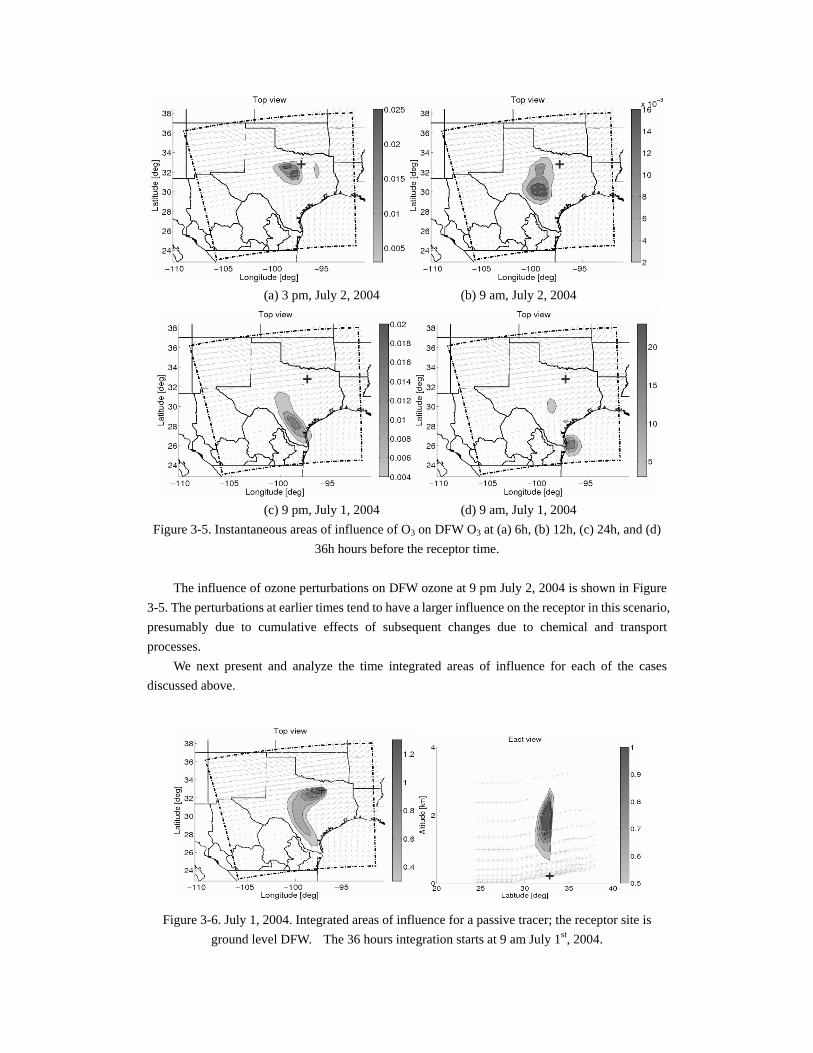
Figure 3-5. Instantaneous areas of influence of O3 on DFW O3 at (a) 6h, (b) 12h, (c) 24h, and (d) 36h hours before the receptor time.

The influence of ozone perturbations on DFW ozone at 9 pm July 2, 2004 is shown in Figure

3-5. The perturbations at earlier times tend to have a larger influence on the receptor in this scenario, presumably due to cumulative effects of subsequent changes due to chemical and transport processes.

We next present and analyze the time integrated areas of influence for each of the cases discussed above.

Figure 3-6. July 1, 2004. Integrated areas of influence for a passive tracer; the receptor site is ground level DFW. The 36 hours integration starts at 9 am July 1st, 2004.

The integrated area of influence for the passive tracer shown in Figure 3-6 reveals the effect of

meteorological conditions on July 1st (independent of the effects of chemistry). The effects trace a corridor going South over central Texas. A tracer perturbation of 1 ppb at a given location (added hourly throughout the simulation interval) would result in a perturbation of the tracer concentration at the receptor equal to the adjoint variable magnitude (gray-coded). Due to vertical mixing and transport the maximum influence region is reported above and slightly west of DFW. Note that this region is near the boundary between the free troposphere and the Planetary Boundary Layer (PBL) at around 2 km, indicating the important role of subsidence.

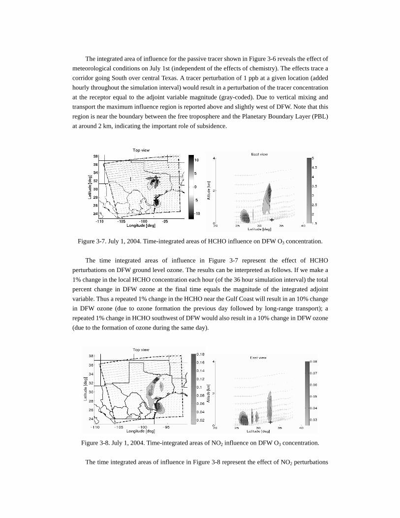
Figure 3-7. July 1, 2004. Time-integrated areas of HCHO influence on DFW O3 concentration.

The time integrated areas of influence in Figure 3-7 represent the effect of HCHO perturbations on DFW ground level ozone. The results can be interpreted as follows. If we make a 1% change in the local HCHO concentration each hour (of the 36 hour simulation interval) the total percent change in DFW ozone at the final time equals the magnitude of the integrated adjoint variable. Thus a repeated 1% change in the HCHO near the Gulf Coast will result in an 10% change in DFW ozone (due to ozone formation the previous day followed by long-range transport); a repeated 1% change in HCHO southwest of DFW would also result in a 10% change in DFW ozone (due to the formation of ozone during the same day).

Figure 3-8. July 1, 2004. Time-integrated areas of NO2 influence on DFW O3 concentration.

The time integrated areas of influence in Figure 3-8 represent the effect of NO2 perturbations

on DFW ground level ozone. There are two areas of maximum influence, where 1% changes in the NO2 concentration introduced every hour result in DFW ozone concentration changes of over 0.15%. One area is near the Gulf Coast; changes in NO2 the previous day result in ozone formation, which is then transported to DFW. The second area is near DFW; local NO2 changes result in O3 changes during the same day.

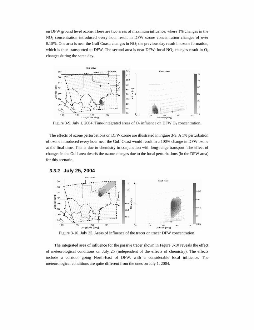
Figure 3-9. July 1, 2004. Time-integrated areas of O3 influence on DFW O3 concentration.

The effects of ozone perturbations on DFW ozone are illustrated in Figure 3-9. A 1% perturbation

of ozone introduced every hour near the Gulf Coast would result in a 100% change in DFW ozone at the final time. This is due to chemistry in conjunction with long-range transport. The effect of changes in the Gulf area dwarfs the ozone changes due to the local perturbations (in the DFW area) for this scenario.

3.3.2 July 25, 2004

Figure 3-10. July 25. Areas of influence of the tracer on tracer DFW concentration.

The integrated area of influence for the passive tracer shown in Figure 3-10 reveals the effect

of meteorological conditions on July 25 (independent of the effects of chemistry). The effects include a corridor going North-East of DFW, with a considerable local influence. The meteorological conditions are quite different from the ones on July 1, 2004.

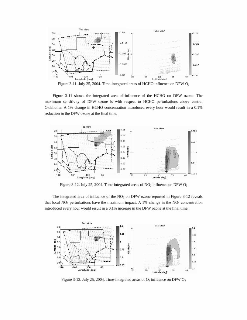
Figure 3-11. July 25, 2004. Time-integrated areas of HCHO influence on DFW O3

Figure 3-11 shows the integrated area of influence of the HCHO on DFW ozone. The

maximum sensitivity of DFW ozone is with respect to HCHO perturbations above central Oklahoma. A 1% change in HCHO concentration introduced every hour would result in a 0.1% reduction in the DFW ozone at the final time.

Figure 3-12. July 25, 2004. Time-integrated areas of NO2 influence on DFW O3

The integrated area of influence of the NO2 on DFW ozone reported in Figure 3-12 reveals that local NO2 perturbations have the maximum impact. A 1% change in the NO2 concentration introduced every hour would result in a 0.1% increase in the DFW ozone at the final time.

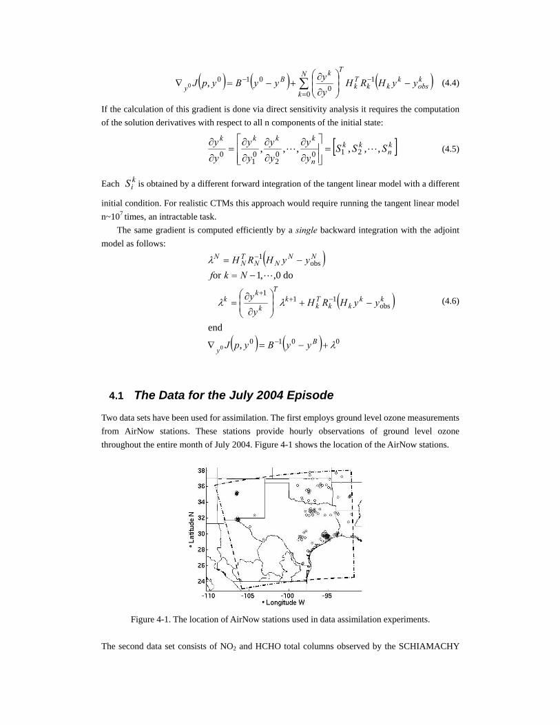
Figure 3-13. July 25, 2004. Time-integrated areas of O3 influence on DFW O3

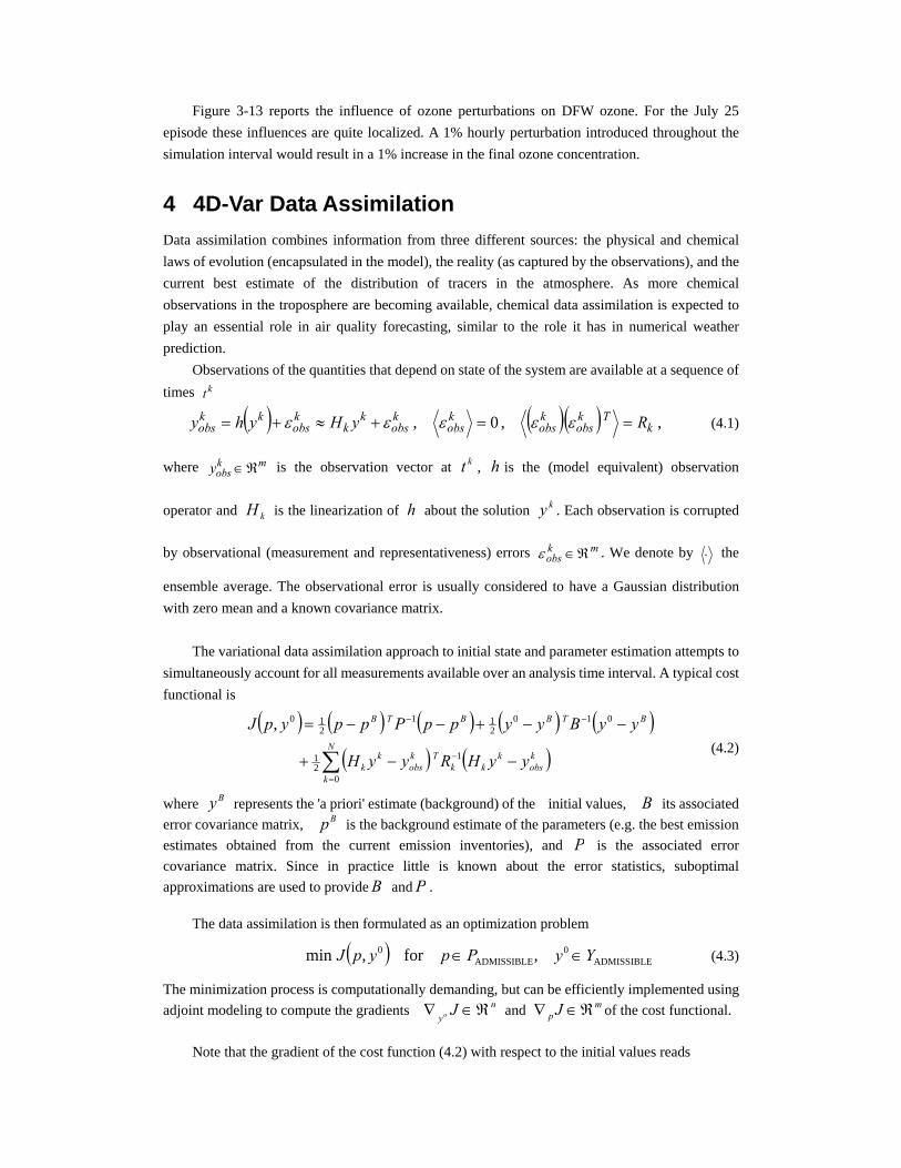
Figure 3-13 reports the influence of ozone perturbations on DFW ozone. For the July 25 episode these influences are quite localized. A 1% hourly perturbation introduced throughout the simulation interval would result in a 1% increase in the final ozone concentration.

4 4D-Var Data Assimilation Data assimilation combines information from three different sources: the physical and chemical laws of evolution (encapsulated in the model), the reality (as captured by the observations), and the current best estimate of the distribution of tracers in the atmosphere. As more chemical observations in the troposphere are becoming available, chemical data assimilation is expected to play an essential role in air quality forecasting, similar to the role it has in numerical weather prediction.

Observations of the quantities that depend on state of the system are available at a sequence of times kt

( ) ( )( ) ,,0, kTk

obskobs

kobs

kobs

kk

kobs

kkobs RyHyhy ==+≈+= εεεεε (4.1)

where mkobsy ℜ∈ is the observation vector at kt , h is the (model equivalent) observation

operator and kH is the linearization of h about the solution ky . Each observation is corrupted

by observational (measurement and representativeness) errors mkobs ℜ∈ε . We denote by ⋅ the

ensemble average. The observational error is usually considered to have a Gaussian distribution with zero mean and a known covariance matrix.

The variational data assimilation approach to initial state and parameter estimation attempts to simultaneously account for all measurements available over an analysis time interval. A typical cost functional is

( ) ( ) ( ) ( ) ( )( ) ( )∑

=

−

−−

−−+

−−+−−=N

k

kobs

kkk

Tkobs

kk

BTBBTB

yyHRyyH

yyByyppPppypJ

0

121

010211

210,

(4.2)

where By represents the 'a priori' estimate (background) of the initial values, B its associated error covariance matrix, Bp is the background estimate of the parameters (e.g. the best emission estimates obtained from the current emission inventories), and P is the associated error covariance matrix. Since in practice little is known about the error statistics, suboptimal approximations are used to provide B and P .

The data assimilation is then formulated as an optimization problem

( ) ADMISSIBLE0

ADMISSIBLE0 ,for,min YyPpypJ ∈∈ (4.3)

The minimization process is computationally demanding, but can be efficiently implemented using adjoint modeling to compute the gradients n

y Jo ℜ∈∇ and mp J ℜ∈∇ of the cost functional.

Note that the gradient of the cost function (4.2) with respect to the initial values reads

( ) ( ) ( )∑=

−− −⎟⎟⎠

⎞⎜⎜⎝

⎛

∂

∂+−=∇

N

k

kobs

kkk

Tk

TkB

y yyHRHyyyyBypJ

0

10

010,0 (4.4)

If the calculation of this gradient is done via direct sensitivity analysis it requires the computation of the solution derivatives with respect to all n components of the initial state:

[ ]kn

kk

n

kkkkSSS

yy

yy

yy

yy ,,,,,, 2100

201

0 LL =⎥⎥⎦

⎤

⎢⎢⎣

⎡

∂

∂

∂

∂

∂

∂=

∂

∂ (4.5)

Each kiS is obtained by a different forward integration of the tangent linear model with a different

initial condition. For realistic CTMs this approach would require running the tangent linear model n~107 times, an intractable task.

The same gradient is computed efficiently by a single backward integration with the adjoint model as follows:

( )

( )

( ) ( ) 0010

obs11

1

obs1

,

end

do0,,1or

0 λ

λλ

λ

+−=∇

−+⎟⎟⎠

⎞⎜⎜⎝

⎛

∂

∂=

−=−=

−

−++

−

By

kkkk

Tk

kT

k

kk

NNNN

TN

N

yyBypJ

yyHRHy

y

NkfyyHRH

L

(4.6)

4.1 The Data for the July 2004 Episode

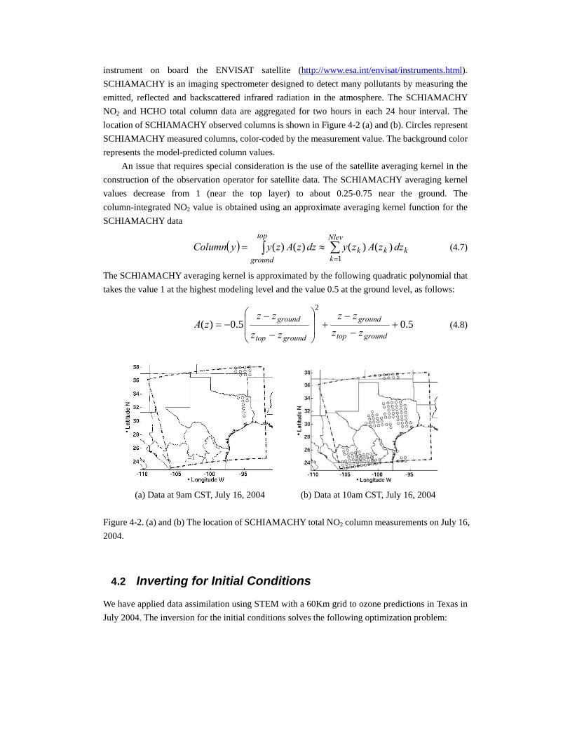
Two data sets have been used for assimilation. The first employs ground level ozone measurements from AirNow stations. These stations provide hourly observations of ground level ozone throughout the entire month of July 2004. Figure 4-1 shows the location of the AirNow stations.

Figure 4-1. The location of AirNow stations used in data assimilation experiments.

The second data set consists of NO2 and HCHO total columns observed by the SCHIAMACHY

instrument on board the ENVISAT satellite (http://www.esa.int/envisat/instruments.html). SCHIAMACHY is an imaging spectrometer designed to detect many pollutants by measuring the emitted, reflected and backscattered infrared radiation in the atmosphere. The SCHIAMACHY NO2 and HCHO total column data are aggregated for two hours in each 24 hour interval. The location of SCHIAMACHY observed columns is shown in Figure 4-2 (a) and (b). Circles represent SCHIAMACHY measured columns, color-coded by the measurement value. The background color represents the model-predicted column values.

An issue that requires special consideration is the use of the satellite averaging kernel in the construction of the observation operator for satellite data. The SCHIAMACHY averaging kernel values decrease from 1 (near the top layer) to about 0.25-0.75 near the ground. The column-integrated NO2 value is obtained using an approximate averaging kernel function for the SCHIAMACHY data

( ) kk

Nlev

kk

top

grounddzzAzydzzAzyyColumn )()()()(

1∑∫=

≈= (4.7)

The SCHIAMACHY averaging kernel is approximated by the following quadratic polynomial that takes the value 1 at the highest modeling level and the value 0.5 at the ground level, as follows:

5.05.0)(

2

+−

−+⎟

⎟

⎠

⎞

⎜⎜

⎝

⎛

−

−−=

groundtop

ground

groundtop

ground

zzzz

zz

zzzA (4.8)

(a) Data at 9am CST, July 16, 2004 (b) Data at 10am CST, July 16, 2004

Figure 4-2. (a) and (b) The location of SCHIAMACHY total NO2 column measurements on July 16, 2004.

4.2 Inverting for Initial Conditions

We have applied data assimilation using STEM with a 60Km grid to ozone predictions in Texas in July 2004. The inversion for the initial conditions solves the following optimization problem:

( ) ( ) ( )( ) ( )∑

=

−

−

−−+

−−=N

k

kobs

kkk

Tkobs

kk

BTB

yyHRyyH

yyByyyJ

0

121

010210min

(4.9)

where the control variables are the initial concentrations of 50 different chemical species.

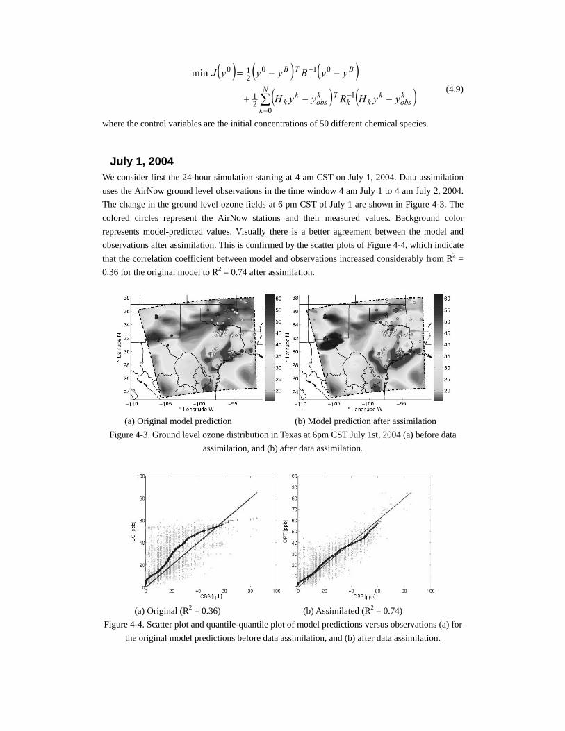
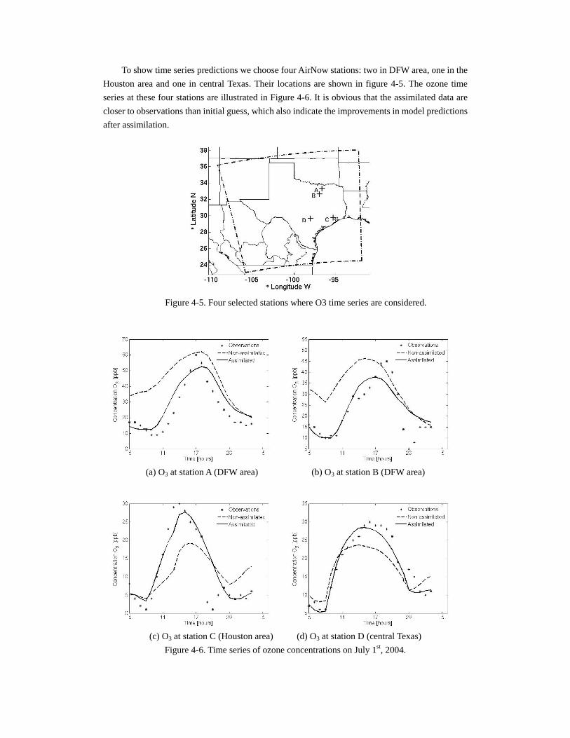
July 1, 2004 We consider first the 24-hour simulation starting at 4 am CST on July 1, 2004. Data assimilation uses the AirNow ground level observations in the time window 4 am July 1 to 4 am July 2, 2004. The change in the ground level ozone fields at 6 pm CST of July 1 are shown in Figure 4-3. The colored circles represent the AirNow stations and their measured values. Background color represents model-predicted values. Visually there is a better agreement between the model and observations after assimilation. This is confirmed by the scatter plots of Figure 4-4, which indicate that the correlation coefficient between model and observations increased considerably from R2 = 0.36 for the original model to R2 = 0.74 after assimilation.

(a) Original model prediction (b) Model prediction after assimilation

Figure 4-3. Ground level ozone distribution in Texas at 6pm CST July 1st, 2004 (a) before data assimilation, and (b) after data assimilation.

(a) Original (R2 = 0.36) (b) Assimilated (R2 = 0.74) Figure 4-4. Scatter plot and quantile-quantile plot of model predictions versus observations (a) for

the original model predictions before data assimilation, and (b) after data assimilation.

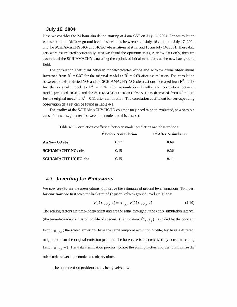
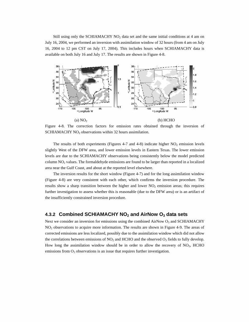
To show time series predictions we choose four AirNow stations: two in DFW area, one in the Houston area and one in central Texas. Their locations are shown in figure 4-5. The ozone time series at these four stations are illustrated in Figure 4-6. It is obvious that the assimilated data are closer to observations than initial guess, which also indicate the improvements in model predictions after assimilation.

Figure 4-5. Four selected stations where O3 time series are considered.

(a) O3 at station A (DFW area) (b) O3 at station B (DFW area)

(c) O3 at station C (Houston area) (d) O3 at station D (central Texas)

Figure 4-6. Time series of ozone concentrations on July 1st, 2004.

July 16, 2004 Next we consider the 24-hour simulation starting at 4 am CST on July 16, 2004. For assimilation we use both the AirNow ground level observations between 4 am July 16 and 4 am July 17, 2004 and the SCHIAMACHY NO2 and HCHO observations at 9 am and 10 am July 16, 2004. These data sets were assimilated sequentially: first we found the optimum using AirNow data only, then we assimilated the SCHIAMACHY data using the optimized initial conditions as the new background field.

The correlation coefficient between model-predicted ozone and AirNow ozone observations increased from R2 = 0.37 for the original model to R2 = 0.69 after assimilation. The correlation between model-predicted NO2 and the SCHIAMACHY NO2 observations increased from R2 = 0.19 for the original model to R2 = 0.36 after assimilation. Finally, the correlation between model-predicted HCHO and the SCHIAMACHY HCHO observations decreased from R2 = 0.19 for the original model to R2 = 0.11 after assimilation. The correlation coefficient for corresponding observation data set can be found in Table 4-1.

The quality of the SCHIAMACHY HCHO columns may need to be re-evaluated, as a possible cause for the disagreement between the model and this data set.

Table 4-1. Correlation coefficient between model prediction and observations

R2 Before Assimilation R2 After Assimilation

AirNow O3 obs 0.37 0.69

SCHIAMACHY NO2 obs 0.19 0.36

SCHIAMACHY HCHO obs 0.19 0.11

4.3 Inverting for Emissions

We now seek to use the observations to improve the estimates of ground level emissions. To invert for emissions we first scale the background (a priori values) ground level emissions:

),,(),,( ,, tyxEtyxE jiBssjijis α= (4.10)

The scaling factors are time-independent and are the same throughout the entire simulation interval

(the time-dependent emission profile of species s at location ),( ji yx is scaled by the constant

factor sji ,,α ; the scaled emissions have the same temporal evolution profile, but have a different

magnitude than the original emission profile). The base case is characterized by constant scaling

factor 1,, =sjiα . The data assimilation process updates the scaling factors in order to minimize the

mismatch between the model and observations.

The minimization problem that is being solved is:

( ) ( ) ( ) ( )( ) ( )

maxmin

0

121

22

121 111min

ααα

αααα γ

≤≤

−−+

−Δ+−−=

∑=

−

−

tosubject

N

k

kobs

kkk

Tkobs

kk

T

yyHRyyH

PJ

(4.11)

The first term is the “background term” in 4D-Var and penalizes the departure of the scaling factors from the “best guess” value of 1. The second term is a regularization term. The Laplacian of the

scaling factor ( 2222 // yx ∂∂+∂∂=Δ ) is large if the scaling factor changes a lot from one location

to another. The introduction of the regularization term in the cost functional will thus favor a smooth spatial profile of the correction factors, by penalizing jumps in the profile value. The strength of the penalty is given by the (adjustable) constantγ . The last term in the cost function measures the mismatch between model predictions and observations. The correction factors are

restricted to an interval ],[ maxmin αα which is predetermined to contain “reasonable” correction

values. All the data assimilation experiments presented in this section use the optimized initial

conditions (previously obtained). The minimization only adjusts the emission rates of selected species (NO2, and HCHO). Thus our approach is to first optimize for initial conditions, and then optimize for emissions.

4.3.1 SCHIAMACHY NO2 data set We first performed an inversion using only the SCHIAMACHY NO2 data set. The assimilation window is 8 hours (4 am to 12 pm CST on July 16, 2004) and includes both hours when SCHIAMACHY data is available on July 16. The initial conditions at 4 am are the ones obtained from the previous optimization. The emission correction coefficients are limited to the range

22.0 ≤≤ α . The results are shown in Figure 4-7, and indicate higher NO2 emissions slightly west of the DFW area and over Oklahoma, and lower emissions in southeast Texas. Higher HCHO emissions are indicated in localized areas.

(a) NO2 (b) HCHO

Figure 4-7. The correction factors for emission rates obtained through the inversion of SCHIAMACHY NO2 observations within 8 hours assimilation.

Still using only the SCHIAMACHY NO2 data set and the same initial conditions at 4 am on

July 16, 2004, we performed an inversion with assimilation window of 32 hours (from 4 am on July 16, 2004 to 12 pm CST on July 17, 2004). This includes hours when SCHIAMACHY data is available on both July 16 and July 17. The results are shown in Figure 4-8.

(a) NO2 (b) HCHO Figure 4-8. The correction factors for emission rates obtained through the inversion of SCHIAMACHY NO2 observations within 32 hours assimilation.

The results of both experiments (Figures 4-7 and 4-8) indicate higher NO2 emission levels slightly West of the DFW area, and lower emission levels in Eastern Texas. The lower emission levels are due to the SCHIAMACHY observations being consistently below the model predicted column NO2 values. The formaldehyde emissions are found to be larger than reported in a localized area near the Gulf Coast, and about at the reported level elsewhere.

The inversion results for the short window (Figure 4-7) and for the long assimilation window (Figure 4-8) are very consistent with each other, which confirms the inversion procedure. The results show a sharp transition between the higher and lower NO2 emission areas; this requires further investigation to assess whether this is reasonable (due to the DFW area) or is an artifact of the insufficiently constrained inversion procedure.

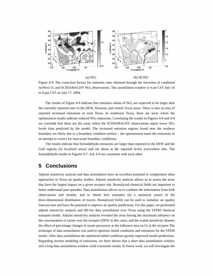
4.3.2 Combined SCHIAMACHY NO2 and AirNow O3 data sets Next we consider an inversion for emissions using the combined AirNow O3 and SCHIAMACHY NO2 observations to acquire more information. The results are shown in Figure 4-9. The areas of corrected emissions are less localized, possibly due to the assimilation window which did not allow the correlations between emissions of NO2 and HCHO and the observed O3 fields to fully develop. How long the assimilation window should be in order to allow the recovery of NO2, HCHO emissions from O3 observations is an issue that requires further investigation.

(a) NO2 (b) HCHO

Figure 4-9. The correction factors for emission rates obtained through the inversion of combined AirNow O3 and SCHIAMACHY NO2 observations. The assimilation window is 4 am CST July 16 to 8 pm CST on July 17, 2004.

The results of Figure 4-9 indicate that emission values of NO2 are expected to be larger than the currently reported ones in the DFW, Houston, and central Texas areas. There is also an area of reported increased emissions in west Texas. In southwest Texas, there are areas where the optimization results indicate reduced NO2 emissions. Correlating the results in Figures 4-8 and 4-9 we conclude that these are the areas where the SCHIAMACHY observations report lower NO2 levels than predicted by the model. The increased emission regions found near the northern boundary are likely due to a boundary condition artifact – the optimization tunes the emissions in an attempt to correct for inaccurate boundary conditions.

The results indicate that formaldehyde emissions are larger than reported in the DFW and the Gulf regions (in localized areas) and are about at the reported levels everywhere else. The formaldehyde results in Figures 4-7, 4-8, 4-9 are consistent with each other.

5 Conclusions Adjoint sensitivity analysis and data assimilation have an excellent potential to complement other approaches in Texas air quality studies. Adjoint sensitivity analysis allows us to assess the areas that have the largest impact on a given receptor site. Reanalyzed chemical fields are important to better understand past episodes. Data assimilation allows us to combine the information from both observations and models, and to obtain best estimates (in a statistical sense) of the three-dimensional distribution of tracers. Reanalyzed fields can be used to initialize air quality forecast runs and have the potential to improve air quality predictions. For this paper, we performed adjoint sensitivity analysis and 4D-Var data assimilation over Texas using the STEM chemical transport model. Adjoint sensitivity analysis revealed the areas having the maximum influence on the concentration of ozone over the receptor (DFW in this case), and the scaled sensitivity denotes the effect of percentage changes in ozone precursors at the influence area on O3 at the receptor The technique of data assimilation was used to optimize initial conditions and emissions for the STEM model. After data assimilation the optimized initial conditions greatly improved model predictions. Regarding inverse modeling of emissions, we have shown that a short data assimilation window and a long data assimilation window yield consistent results. In future work, we will investigate the

assimilation window times required to allow the recovery of NO2 and HCHO emissions from O3 observations, and the reasons for the sharp transition between areas requiring higher adjusted emissions and those requiring lower adjusted emissions. Acknowledgements. This work has been supported by the Houston Advanced Research Council through the award H59/2005. Zhang, Constantinescu, Sandu, Chai, and Carmichael were also supported by NSF through the award NSF ITR 0205198.

6 REFERENCES [1] D.G.Cacuci. Sensitivity theory for nonlinear systems. I. Nonlinear functional analysis approach. J. Math.

Phys., 22:2794-2802, 1981.

[2] D.G.Cacuci. Sensitivity theory for nonlinear systems. II. Extensions to additional classes of responses. J. Math.

Phys., 22:2803-2812, 1981.

[3] A.M. Dunker. The decoupled direct method for calculating sensitivity coefficients in chemical kinetics, J.

Chem. Phy., 81, 2385-2393, 1984.

[4] A. Sandu, D.N. Daescu, G.R. Carmichael, and T. Chai. Adjoint Sensitivity Analysis of Regional Air Quality

Models. Journal of Computational Physics, Vol. 204, p. 222-252, 2005.

[5] D.K. Henze and J.H. Seinfeld. Development of the adjoint of GEOS-Chem. Atomospheric Chemistry and

Physics Discussions., 6, 10591-10648, 2006.

[6] G.I. Marchuk. Adjoint Equations and Analysis of Complex Systems. Kluwer Academic Publishers, 1995.

[7] G.I. Marchuk, P.V. Agoshkow, and I.V. Shutyaev. Adjoint Equations and Perturbation Algorithms in

Nonlinear Problems. CRC Press, 1996.

[8] M. Fisher and D.J. Lary. Lagrangian four-dimensional variational data assimilation of chemical species. Q.J.R.

Meteorology, 121:1681-1704, 1995.

[9] B.V. Khattatov, J.C. Gille, L.V. Lyjak, G.P. Brasseur, V.L. Dvortsov, A.E. Roche, and J. Walters. Assimilation

of photochemically active species and a case analysis of UARS data. Journal of Geophysical Research,

104:18715-18737, 1999.

[10] H.Elbern, H. Schmidt, and A. Ebel. Variational data assimilation for tropospheric chemistry modeling. Journal

of Geophysical Research, 102(D13):15967-15985, 1997.

[11] H. Elbern and H. Schmidt. A 4D-Var chemistry data assimilation scheme for Eulerian chemistry transport

modeling. Journal of Geophysical Research, 104(5):18583-18598, 1999.

[12] Q. Errera and D. Fonteyn. Four-dimensional variational chemical assimilation of CRISTA stratospheric

measurements. Journal of Geophysical Research, 106(D11):12253-12265, 2001.

[13] K.Y. Wang, D.J. Lary, D.E. Shallcross, Hall S.M., and Pyle J.A. A review on the use of the adjoint method in

four-dimensional atmospheric-chemistry data assimilation. Q.J.R. Meteorol. Soc., 127(576(Part

B)):2181-2204, 2001.

[14] H. Elbern and H. Schmidt, O. Talagrand, and A. Ebel. 4D-variational data assimilation with an adjoint air

quality model for emission analysis. Environmental Modeling and Software, 15:539-548, 2000.

[15] H. Elbern and H. Schmidt. Ozone episode analysis by 4D-Var chemistry data assimilation. Journal of

Geophysical Research, 106(D4):3569-3590, 2001.

[16] Y. Tang, et al. (2003a), Impacts of aerosols and clouds on photolysis frequencies and photochemistry during

TRACE-P: 2. Three-dimensional study using a regional chemical transport model. Journal of Geophysical

Research, 108(D21), 8822, doi: 10.1029/2002JD003100

[17] G.R. Carmichael, et al. (2003a), Regional-scale chemical transport modeling in support of the analysis of

observations obtained during the TRACE-P experiment. Journal of Geophysical Research, 108(D21), 8823,

doi:10.1029/2002JD003117.

[18] W.P.L. Carter. Documentation of the SPARC-99 chemical mechanism for VOC reactivity assessment final

report to California Air Resources Board. Technical Report. University of California at Riverside, 2000.

[19] Y.P. Kim, J. H. Seinfeld, and P. Saxena (1993a). Atmospheric gas-aerosol equilibrium. I: Thermodynamic

model, Aerosol Sci. Technol, 19, 151 – 181.

[20] Y.P. Kim, J.H. Seinfeld, and P. Saxena (1993b). Atmospheric gas-aerosol equilibrium. II: Analysis of common

approximations and activity coefficient calculation methods, Aerosol Sci. Technol, 19, 182-198.

[21] Y. Tang, et al. (2004), Three-dimensional simulations of inorganic aerosol distributions in east Asia during

spring 2001, Journal of Geophysical Research, 109, doi: 10.1029/2003JD004201.