direct and adjoint sensitivity analysis ofchemical...

Atmospheric Environment 37 (2003) 5097–5114

ARTICLE IN PRESS

*Correspondin

319-335-3337.

E-mail addre

[email protected]

(G.R. Carmicha

1352-2310/$ - see

doi:10.1016/j.atm

Direct and adjoint sensitivity analysis of chemical kineticsystems with KPP: II—numerical validation and applications

Dacian N. Daescua, Adrian Sandub, Gregory R. Carmichaelc,*a Institute for Mathematics and its Applications, University of Minnesota, 400 Lind Hall 207 Church Street S.E., Minneapolis,

MN 55455, USAbDepartment of Computer Science, Virginia Polytechnic Institute and State University, 660 McBryde Hall, Blacksburg, VA 24061, USA

c Center for Global and Regional Environmental Research, 204 IATL, The University of Iowa, Iowa City, IA 52242-1297, USA

Received 26 January 2003; accepted 7 August 2003

Abstract

The Kinetic PreProcessor KPP was extended to generate the building blocks needed for the direct and adjoint

sensitivity analysis of chemical kinetic systems. An overview of the theoretical aspects of sensitivity calculations and a

discussion of the KPP software tools is presented in the companion paper.

In this work the correctness and efficiency of the KPP generated code for direct and adjoint sensitivity studies are

analyzed through an extensive set of numerical experiments. Direct-decoupled Rosenbrock methods are shown to be

cost-effective for providing sensitivities at low and medium accuracies. A validation of the discrete–adjoint evaluated

gradients is performed against the finite difference estimates. The accuracy of the adjoint gradients is measured using a

reference gradient value obtained with a standard direct-decoupled method. The accuracy is studied for both constant

step size and variable step size integration of the forward/adjoint model and the consistency between the discrete and

continuous adjoint models is analyzed.

Applications of the KPP-1.2 software package to direct and adjoint sensitivity studies, variational data assimilation,

and parameter identification are considered for the comprehensive chemical mechanism SAPRC-99.

r 2003 Elsevier Ltd. All rights reserved.

Keywords: Sensitivity analysis; Data assimilation; Parameter identification; Optimization

1. Introduction

The direct-decoupled method and the adjoint method

are powerful tools for sensitivity analysis. Currently,

several commercial software packages such as SENKIN

(Lutz et al., 1987) and LSENS (Radhakrishnan, 2003)

implement the direct-decoupled method for the sensitiv-

ity analysis of gas-phase chemical reactions. Given a

chemical kinetics system described by a list of chemical

reactions, the Kinetic PreProcessor KPP (Damian-

g author. Tel.: +1-319-335-3333; fax: +1-

sses: [email protected] (D.N. Daescu),

u (A. Sandu), [email protected]

el).

front matter r 2003 Elsevier Ltd. All rights reserve

osenv.2003.08.020

Iordache et al., 2002) generates the FORTRAN 77 or

C code for the forward model integration and sub-

routines that allow direct-decoupled/adjoint sensitivity

analysis with minimal user intervention. The capability

to implement the continuous/discrete adjoint sensitivity

analysis represents a major contribution of the new

release KPP-1.2.

An overview of the theoretical aspects of sensitivity

calculations and a discussion of the KPP software tools

is presented in the companion paper (Sandu et al., 2003).

In this paper, we present an extensive set of numerical

experiments and applications of the KPP software to

sensitivity studies for chemical kinetics systems.

Our tests use the SAPRC-99 atmospheric chemistry

mechanism (Carter, 2000a, b) which considers the

gas-phase atmospheric reactions of volatile organic

d.

ARTICLE IN PRESSD.N. Daescu et al. / Atmospheric Environment 37 (2003) 5097–51145098

compounds (VOCs) and nitrogen oxides ðNOxÞ in urban

and regional settings. The chemical mechanism was

developed at University of California, Riverside by Dr.

W.P.L. Carter for use in airshed models for predicting

the effects of VOC and NOx emissions on tropospheric

secondary pollutants formation such as ozone ðO3Þ and

other oxidants. In our analysis we consider the

condensed fixed-parameter version of the SAPRC-99

mechanism (Carter, 2000a) which is suitable for

implementation into the Models-3 software framework.

This version takes into consideration 211 reactions

among 74 variable chemical species (in addition O2, H2,

CH4, and H2O concentrations are considered fixed),

and is currently incorporated into the three-dimensional

regional-scale model STEM-II (Carmichael et al., 1986).

A list of the variable chemical species in the model is

presented in Table 1.

In Section 2 we present the numerical solvers available

in the KPP library for direct-decoupled and discrete/

continuous adjoint sensitivity calculations. Experimen-

tal settings, the forward model integration, and issues

related to the sparse linear algebra computations are

discussed. Direct sensitivity calculations with respect to

initial conditions and to reaction rate coefficients using

Rosenbrock solvers up to order four are presented in

Section 3. The accuracy and the efficiency of the direct-

decoupled method is analyzed. Section 4 is dedicated to

adjoint sensitivity analysis. Adjoint model validation,

consistency between the discrete and adjoint model, and

accuracy issues are discussed. The computational

expense and the efficiency of the adjoint model are

investigated. Applications are presented for time-depen-

dent sensitivities with respect to the model state, reaction

rate coefficients, and emissions. In Section 5 we present

applications of the adjoint modeling to variational data

assimilation and parameter estimation using the initial

conditions and emission rates as control variables.

Concluding remarks and future research directions are

presented in Section 6.

2. Numerical solvers

The dynamical model associated with the chemical

mechanism is given by a system of nonlinear ordinary

differential equations (ODEs)

dy

dt¼ f ðyÞ þ E; ð1Þ

where yARn is the vector of concentrations, f ðyÞ is the

chemical production/loss function, and EARn represents

the vector of emission rates (Ei ¼ 0 if there are no

emissions of species i). Throughout this paper an upper

index will specify the discrete time moment and a lower

index will specify the vector component. For example, yi

is the concentration vector at time ti and yj denotes the

jth component of the vector y:Due to the wide range of characteristic time scales of

the chemical reactions, the eigenvalues of the Jacobian

matrix J ¼ @f =@y may differ by several orders of

magnitude. Such systems are usually referred to as

being ‘‘stiff’’ (Aiken, 1985). Explicit numerical methods

are usually impractical to integrate stiff systems since

may exhibit a severe restriction of the step size. For this

reason, numerical schemes that are particularly suitable

for integrating stiff ODE systems have been developed

(Aiken, 1985; Hairer and Wanner, 1991).

Rosenbrock methods (Hairer and Wanner, 1991) are

well-suited for atmospheric chemistry applications

(Sandu et al., 1997) due to their optimal stability

properties and conservation of the linear invariants of

the system (e.g. they are mass-conservative). When the

sparsity of the ODE system is carefully exploited,

Rosenbrock methods can efficiently integrate atmo-

spheric chemistry systems. The accuracy requirements in

atmospheric transport-chemistry models are modest

(1%) such that low-order methods are usually em-

ployed. For the numerical experiments we consider the

second-order two-stage L-stable solver ROS2 (Verwer

et al., 1999) and the third-order four-stage stiffly

accurate solver RODAS3 (Sandu et al., 1997). Both

integrators use variable step size for error control and

the forward, discrete, and continuous adjoint model

integrations have been implemented using the KPP

software tools. The derivation of the discrete adjoint

formulae follows our previous work (Daescu et al.,

2000). Two other methods presented by Hairer and

Wanner (1991) are included in the KPP-1.2 numerical

library: the linearly-implicit Euler method (one-stage

Rosenbrock) implemented with constant step size is

available in forward/adjoint mode for testing purposes

only, and the fourth-order four-stage L-stable solver

ROS4 is available for direct-decoupled sensitivity.

2.1. Experimental settings

For the numerical experiments we selected a pollution

scenario with urban VOC and high NOx levels using

input data and reaction rate constants from Carter

(2000a) MD3TEST2, as follows: the model simulation

starts at local noon ðts ¼ 12:00LTÞ with the concentra-

tion of all variable chemical species set to zero.

Emissions are prescribed at constant rates for 30

chemical species in the model as specified in Table 2

ðErefi Þ: We assume a day time interval from 4:30LT

(sunrise) to 19:30LT (sunset) with the photolysis

reaction rates updated every 15 min; and a constant

temperature of 300 K: The system is integrated for 24 h

and the resulting state y0 at t0 ¼ ts þ 24h is taken as the

initial state of the model for a 5 day run ð120 hÞ: The

ARTICLE IN PRESS

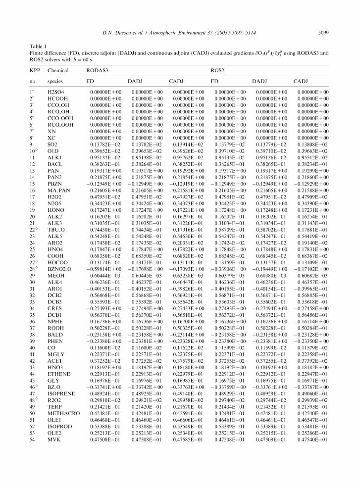
Table 1

Finite difference (FD), discrete adjoint (DADJ) and continuous adjoint (CADJ) evaluated gradients @O3ðtFÞ=@y0i using RODAS3 and

ROS2 solvers with h ¼ 60 s

KPP Chemical RODAS3 ROS2

no. species FD DADJ CADJ FD DADJ CADJ

1w H2SO4 0.00000E+00 0.00000E+00 0.00000E+00 0.00000E+00 0.00000E+00 0.00000E+00

2w HCOOH 0.00000E+00 0.00000E+00 0.00000E+00 0.00000E+00 0.00000E+00 0.00000E+00

3w CCO OH 0.00000E+00 0.00000E+00 0.00000E+00 0.00000E+00 0.00000E+00 0.00000E+00

4w RCO OH 0.00000E+00 0.00000E+00 0.00000E+00 0.00000E+00 0.00000E+00 0.00000E+00

5w CCO OOH 0.00000E+00 0.00000E+00 0.00000E+00 0.00000E+00 0.00000E+00 0.00000E+00

6w RCO OOH 0.00000E+00 0.00000E+00 0.00000E+00 0.00000E+00 0.00000E+00 0.00000E+00

7w XN 0.00000E+00 0.00000E+00 0.00000E+00 0.00000E+00 0.00000E+00 0.00000E+00

8w XC 0.00000E+00 0.00000E+00 0.00000E+00 0.00000E+00 0.00000E+00 0.00000E+00

9 SO2 0.13782E�02 0.13782E�02 0.13914E�02 0.13779E�02 0.13779E�02 0.13808E�02

10} O1D 0.39652E�02 0.39653E�02 0.39626E�02 0.39710E�02 0.39710E�02 0.39663E�02

11 ALK1 0.95137E�02 0.95138E�02 0.95762E�02 0.95135E�02 0.95136E�02 0.95512E�02

12 BACL 0.38263E�01 0.38264E�01 0.38252E�01 0.38265E�01 0.38265E�01 0.38234E�01

13 PAN 0.19317E+00 0.19317E+00 0.19292E+00 0.19317E+00 0.19317E+00 0.19299E+00

14 PAN2 0.21875E+00 0.21875E+00 0.21854E+00 0.21875E+00 0.21875E+00 0.21860E+00

15 PBZN �0.12949E+00 �0.12949E+00 �0.12919E+00 �0.12949E+00 �0.12949E+00 �0.12929E+00

16 MA PAN 0.21605E+00 0.21605E+00 0.21581E+00 0.21605E+00 0.21605E+00 0.21588E+00

17 H2O2 0.47951E�02 0.47951E�02 0.47927E�02 0.47951E�02 0.47951E�02 0.47909E�02

18 N2O5 0.34423E+00 0.34424E+00 0.34373E+00 0.34423E+00 0.34423E+00 0.34390E+00

19 HONO 0.17247E+00 0.17247E+00 0.17221E+00 0.17248E+00 0.17248E+00 0.17231E+00

20 ALK2 0.16202E�01 0.16202E�01 0.16297E�01 0.16202E�01 0.16202E�01 0.16254E�01

21 ALK3 0.31035E�01 0.31035E�01 0.31226E�01 0.31034E�01 0.31034E�01 0.31143E�01

22}� TBU O 0.74430E�01 0.74434E�01 0.17916E�01 0.58709E�01 0.58702E�01 0.17881E�01

23 ALK5 0.54248E�01 0.54248E�01 0.54530E�01 0.54247E�01 0.54247E�01 0.54419E�01

24 ARO2 0.17430E�02 0.17433E�02 0.20331E�02 0.17424E�02 0.17427E�02 0.19140E�02

25 HNO4 0.17847E+00 0.17847E+00 0.17822E+00 0.17848E+00 0.17848E+00 0.17831E+00

26 COOH 0.68350E�02 0.68350E�02 0.68520E�02 0.68345E�02 0.68345E�02 0.68367E�02

27} HOCOO 0.13174E�01 0.13171E�01 0.13111E�01 0.13159E�01 0.13157E�01 0.13109E�01

28}� BZNO2 O �0.59814E+00 �0.17698E+00 �0.17093E+00 �0.33906E+00 �0.19449E+00 �0.17102E+00

29 MEOH 0.60444E�03 0.60445E�03 0.63238E�03 0.60379E�03 0.60380E�03 0.60682E�03

30 ALK4 0.46236E�01 0.46237E�01 0.46447E�01 0.46236E�01 0.46236E�01 0.46357E�01

31 ARO1 �0.40153E�01 �0.40152E�01 �0.39826E�01 �0.40155E�01 �0.40154E�01 �0.39965E�01

32 DCB2 0.56868E�01 0.56868E�01 0.56921E�01 0.56871E�01 0.56871E�01 0.56885E�01

33 DCB3 0.55593E�01 0.55592E�01 0.55642E�01 0.55603E�01 0.55602E�01 0.55618E�01

34 CRES �0.27493E+00 �0.27494E+00 �0.27433E+00 �0.27493E+00 �0.27494E+00 �0.27458E+00

35 DCB1 0.56370E�01 0.56370E�01 0.56510E�01 0.56372E�01 0.56372E�01 0.56456E�01

36 NPHE �0.16736E+00 �0.16736E+00 �0.16700E+00 �0.16736E+00 �0.16736E+00 �0.16714E+00

37 ROOH 0.50228E�01 0.50228E�01 0.50325E�01 0.50228E�01 0.50228E�01 0.50284E�01

38 BALD �0.23158E+00 �0.23158E+00 �0.23114E+00 �0.23158E+00 �0.23158E+00 �0.23128E+00

39 PHEN �0.23380E+00 �0.23381E+00 �0.23328E+00 �0.23380E+00 �0.23381E+00 �0.23350E+00

40 CO 0.11600E�02 0.11600E�02 0.11622E�02 0.11599E�02 0.11599E�02 0.11579E�02

41 MGLY 0.22371E�01 0.22371E�01 0.22375E�01 0.22371E�01 0.22372E�01 0.22358E�01

42 ACET 0.37252E�02 0.37252E�02 0.37579E�02 0.37255E�02 0.37255E�02 0.37392E�02

43 HNO3 0.18192E+00 0.18192E+00 0.18180E+00 0.18192E+00 0.18192E+00 0.18182E+00

44 ETHENE 0.22913E�01 0.22913E�01 0.22979E�01 0.22912E�01 0.22912E�01 0.22947E�01

45 GLY 0.16976E�01 0.16976E�01 0.16985E�01 0.16975E�01 0.16975E�01 0.16971E�01

46} BZ O �0.33741E+00 �0.33742E+00 �0.33763E+00 �0.33759E+00 �0.33761E+00 �0.33787E+00

47 ISOPRENE 0.48924E�01 0.48925E�01 0.49140E�01 0.48929E�01 0.48929E�01 0.49060E�01

48} R2O2 0.29810E�02 0.29821E�02 0.29958E�02 0.29740E�02 0.29744E�02 0.29939E�02

49 TERP 0.21421E�01 0.21420E�01 0.21670E�01 0.21434E�01 0.21432E�01 0.21595E�01

50 METHACRO 0.42481E�01 0.42481E�01 0.42591E�01 0.42481E�01 0.42481E�01 0.42540E�01

51 OLE1 0.46460E�01 0.46460E�01 0.46606E�01 0.46461E�01 0.46461E�01 0.46547E�01

52 ISOPROD 0.53388E�01 0.53388E�01 0.53549E�01 0.53389E�01 0.53389E�01 0.53481E�01

53 OLE2 0.25213E�01 0.25213E�01 0.25340E�01 0.25215E�01 0.25215E�01 0.25286E�01

54 MVK 0.47508E�01 0.47508E�01 0.47585E�01 0.47508E�01 0.47509E�01 0.47540E�01

D.N. Daescu et al. / Atmospheric Environment 37 (2003) 5097–5114 5099

ARTICLE IN PRESS

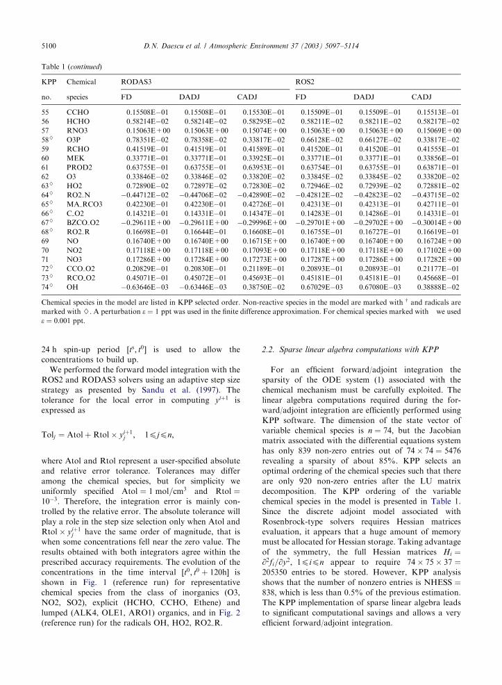
Table 1 (continued)

KPP Chemical RODAS3 ROS2

no. species FD DADJ CADJ FD DADJ CADJ

55 CCHO 0.15508E�01 0.15508E�01 0.15530E�01 0.15509E�01 0.15509E�01 0.15513E�01

56 HCHO 0.58214E�02 0.58214E�02 0.58295E�02 0.58211E�02 0.58211E�02 0.58217E�02

57 RNO3 0.15063E+00 0.15063E+00 0.15074E+00 0.15063E+00 0.15063E+00 0.15069E+00

58}� O3P 0.78351E�02 0.78358E�02 0.33817E�02 0.66128E�02 0.66127E�02 0.33817E�02

59 RCHO 0.41519E�01 0.41519E�01 0.41589E�01 0.41520E�01 0.41520E�01 0.41555E�01

60 MEK 0.33771E�01 0.33771E�01 0.33925E�01 0.33771E�01 0.33771E�01 0.33856E�01

61 PROD2 0.63755E�01 0.63755E�01 0.63953E�01 0.63754E�01 0.63755E�01 0.63871E�01

62 O3 0.33846E�02 0.33846E�02 0.33820E�02 0.33845E�02 0.33845E�02 0.33820E�02

63}� HO2 0.72890E�02 0.72897E�02 0.72830E�02 0.72946E�02 0.72939E�02 0.72881E�02

64}� RO2 N �0.44712E�02 �0.44706E�02 �0.42890E�02 �0.42812E�02 �0.42823E�02 �0.43715E�02

65}� MA RCO3 0.42230E�01 0.42230E�01 0.42726E�01 0.42313E�01 0.42313E�01 0.42711E�01

66} C O2 0.14321E�01 0.14331E�01 0.14347E�01 0.14283E�01 0.14286E�01 0.14331E�01

67}� BZCO O2 �0.29611E+00 �0.29611E+00 �0.29996E+00 �0.29701E+00 �0.29702E+00 �0.30014E+00

68} RO2 R 0.16698E�01 0.16644E�01 0.16608E�01 0.16755E�01 0.16727E�01 0.16619E�01

69 NO 0.16740E+00 0.16740E+00 0.16715E+00 0.16740E+00 0.16740E+00 0.16724E+00

70 NO2 0.17118E+00 0.17118E+00 0.17093E+00 0.17118E+00 0.17118E+00 0.17102E+00

71 NO3 0.17286E+00 0.17284E+00 0.17273E+00 0.17287E+00 0.17286E+00 0.17282E+00

72}� CCO O2 0.20829E�01 0.20830E�01 0.21189E�01 0.20893E�01 0.20893E�01 0.21177E�01

73}� RCO O2 0.45071E�01 0.45072E�01 0.45693E�01 0.45181E�01 0.45181E�01 0.45668E�01

74}� OH �0.63646E�03 �0.63446E�03 0.38750E�02 0.67029E�03 0.67080E�03 0.38888E�02

Chemical species in the model are listed in KPP selected order. Non-reactive species in the model are marked with w and radicals are

marked with }: A perturbation e ¼ 1 ppt was used in the finite difference approximation. For chemical species marked with � we used

e ¼ 0:001 ppt:

D.N. Daescu et al. / Atmospheric Environment 37 (2003) 5097–51145100

24 h spin-up period ½ts; t0� is used to allow the

concentrations to build up.

We performed the forward model integration with the

ROS2 and RODAS3 solvers using an adaptive step size

strategy as presented by Sandu et al. (1997). The

tolerance for the local error in computing yiþ1 is

expressed as

Tolj ¼ Atol þ Rtol � yiþ1j ; 1pjpn;

where Atol and Rtol represent a user-specified absolute

and relative error tolerance. Tolerances may differ

among the chemical species, but for simplicity we

uniformly specified Atol ¼ 1 mol=cm3 and Rtol ¼10�3: Therefore, the integration error is mainly con-

trolled by the relative error. The absolute tolerance will

play a role in the step size selection only when Atol and

Rtol � yiþ1j have the same order of magnitude, that is

when some concentrations fell near the zero value. The

results obtained with both integrators agree within the

prescribed accuracy requirements. The evolution of the

concentrations in the time interval ½t0; t0 þ 120h� is

shown in Fig. 1 (reference run) for representative

chemical species from the class of inorganics (O3,

NO2, SO2), explicit (HCHO, CCHO, Ethene) and

lumped (ALK4, OLE1, ARO1) organics, and in Fig. 2

(reference run) for the radicals OH, HO2, RO2 R.

2.2. Sparse linear algebra computations with KPP

For an efficient forward/adjoint integration the

sparsity of the ODE system (1) associated with the

chemical mechanism must be carefully exploited. The

linear algebra computations required during the for-

ward/adjoint integration are efficiently performed using

KPP software. The dimension of the state vector of

variable chemical species is n ¼ 74; but the Jacobian

matrix associated with the differential equations system

has only 839 non-zero entries out of 74 � 74 ¼ 5476

revealing a sparsity of about 85%. KPP selects an

optimal ordering of the chemical species such that there

are only 920 non-zero entries after the LU matrix

decomposition. The KPP ordering of the variable

chemical species in the model is presented in Table 1.

Since the discrete adjoint model associated with

Rosenbrock-type solvers requires Hessian matrices

evaluation, it appears that a huge amount of memory

must be allocated for Hessian storage. Taking advantage

of the symmetry, the full Hessian matrices Hi ¼@2fi=@y2; 1pipn appear to require 74 � 75 � 37 ¼205350 entries to be stored. However, KPP analysis

shows that the number of nonzero entries is NHESS ¼838; which is less than 0.5% of the previous estimation.

The KPP implementation of sparse linear algebra leads

to significant computational savings and allows a very

efficient forward/adjoint integration.

ARTICLE IN PRESS

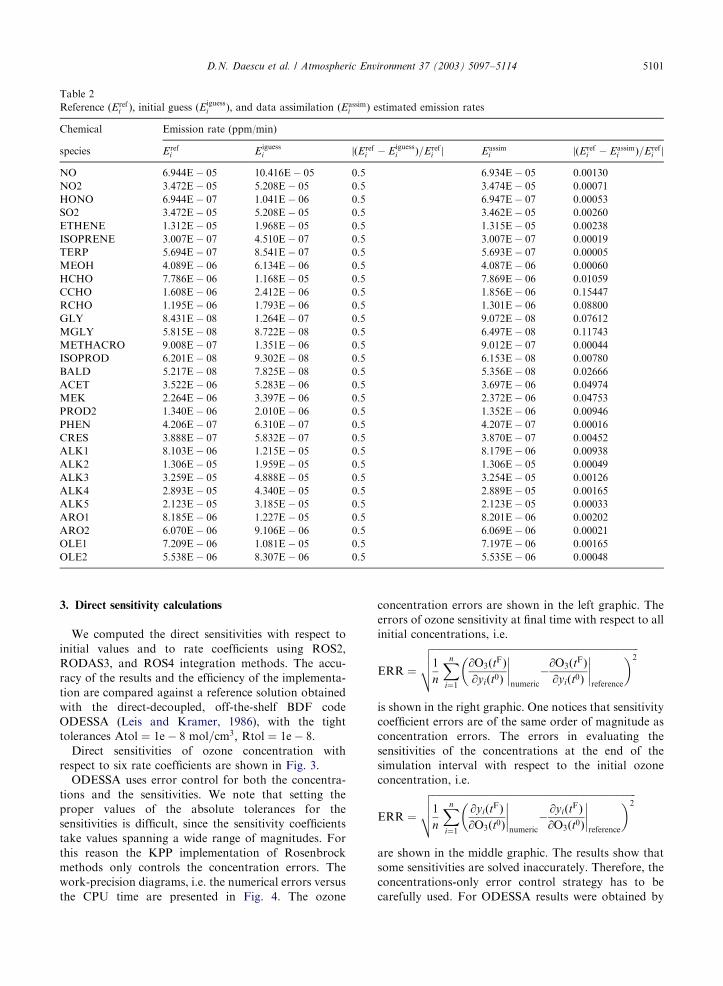
Table 2

Reference ðErefi Þ; initial guess ðEiguess

i Þ; and data assimilation ðEassimi Þ estimated emission rates

Chemical Emission rate (ppm/min)

species Erefi E

iguessi jðEref

i � Eiguessi Þ=Eref

i j Eassimi jðEref

i � Eassimi Þ=Eref

i j

NO 6:944E � 05 10:416E � 05 0.5 6:934E � 05 0.00130

NO2 3:472E � 05 5:208E � 05 0.5 3:474E � 05 0.00071

HONO 6:944E � 07 1:041E � 06 0.5 6:947E � 07 0.00053

SO2 3:472E � 05 5:208E � 05 0.5 3:462E � 05 0.00260

ETHENE 1:312E � 05 1:968E � 05 0.5 1:315E � 05 0.00238

ISOPRENE 3:007E � 07 4:510E � 07 0.5 3:007E � 07 0.00019

TERP 5:694E � 07 8:541E � 07 0.5 5:693E � 07 0.00005

MEOH 4:089E � 06 6:134E � 06 0.5 4:087E � 06 0.00060

HCHO 7:786E � 06 1:168E � 05 0.5 7:869E � 06 0.01059

CCHO 1:608E � 06 2:412E � 06 0.5 1:856E � 06 0.15447

RCHO 1:195E � 06 1:793E � 06 0.5 1:301E � 06 0.08800

GLY 8:431E � 08 1:264E � 07 0.5 9:072E � 08 0.07612

MGLY 5:815E � 08 8:722E � 08 0.5 6:497E � 08 0.11743

METHACRO 9:008E � 07 1:351E � 06 0.5 9:012E � 07 0.00044

ISOPROD 6:201E � 08 9:302E � 08 0.5 6:153E � 08 0.00780

BALD 5:217E � 08 7:825E � 08 0.5 5:356E � 08 0.02666

ACET 3:522E � 06 5:283E � 06 0.5 3:697E � 06 0.04974

MEK 2:264E � 06 3:397E � 06 0.5 2:372E � 06 0.04753

PROD2 1:340E � 06 2:010E � 06 0.5 1:352E � 06 0.00946

PHEN 4:206E � 07 6:310E � 07 0.5 4:207E � 07 0.00016

CRES 3:888E � 07 5:832E � 07 0.5 3:870E � 07 0.00452

ALK1 8:103E � 06 1:215E � 05 0.5 8:179E � 06 0.00938

ALK2 1:306E � 05 1:959E � 05 0.5 1:306E � 05 0.00049

ALK3 3:259E � 05 4:888E � 05 0.5 3:254E � 05 0.00126

ALK4 2:893E � 05 4:340E � 05 0.5 2:889E � 05 0.00165

ALK5 2:123E � 05 3:185E � 05 0.5 2:123E � 05 0.00033

ARO1 8:185E � 06 1:227E � 05 0.5 8:201E � 06 0.00202

ARO2 6:070E � 06 9:106E � 06 0.5 6:069E � 06 0.00021

OLE1 7:209E � 06 1:081E � 05 0.5 7:197E � 06 0.00165

OLE2 5:538E � 06 8:307E � 06 0.5 5:535E � 06 0.00048


3. Direct sensitivity calculations

We computed the direct sensitivities with respect to

initial values and to rate coefficients using ROS2,

RODAS3, and ROS4 integration methods. The accu-

racy of the results and the efficiency of the implementa-

tion are compared against a reference solution obtained

with the direct-decoupled, off-the-shelf BDF code

ODESSA (Leis and Kramer, 1986), with the tight

tolerances Atol ¼ 1e � 8 mol=cm3; Rtol ¼ 1e � 8:Direct sensitivities of ozone concentration with

respect to six rate coefficients are shown in Fig. 3.

ODESSA uses error control for both the concentra-

tions and the sensitivities. We note that setting the

proper values of the absolute tolerances for the

sensitivities is difficult, since the sensitivity coefficients

take values spanning a wide range of magnitudes. For

this reason the KPP implementation of Rosenbrock

methods only controls the concentration errors. The

work-precision diagrams, i.e. the numerical errors versus

the CPU time are presented in Fig. 4. The ozone

concentration errors are shown in the left graphic. The

errors of ozone sensitivity at final time with respect to all

initial concentrations, i.e.

ERR ¼

ffiffiffiffiffiffiffiffiffiffiffiffiffiffiffiffiffiffiffiffiffiffiffiffiffiffiffiffiffiffiffiffiffiffiffiffiffiffiffiffiffiffiffiffiffiffiffiffiffiffiffiffiffiffiffiffiffiffiffiffiffiffiffiffiffiffiffiffiffiffiffiffiffiffiffiffiffiffiffiffiffiffiffi1

n

Xn

i¼1

@O3ðtFÞ@yiðt0Þ

��numeric

�@O3ðtFÞ@yiðt0Þ

��reference

� �2

vuut

is shown in the right graphic. One notices that sensitivity

coefficient errors are of the same order of magnitude as

concentration errors. The errors in evaluating the

sensitivities of the concentrations at the end of the

simulation interval with respect to the initial ozone

concentration, i.e.

ERR ¼

ffiffiffiffiffiffiffiffiffiffiffiffiffiffiffiffiffiffiffiffiffiffiffiffiffiffiffiffiffiffiffiffiffiffiffiffiffiffiffiffiffiffiffiffiffiffiffiffiffiffiffiffiffiffiffiffiffiffiffiffiffiffiffiffiffiffiffiffiffiffiffiffiffiffiffiffiffiffiffiffiffiffi1

n

Xn

i¼1

@yiðtFÞ@O3ðt0Þ

��numeric

�@yiðtFÞ@O3ðt0Þ

��reference

� �2

vuut

are shown in the middle graphic. The results show that

some sensitivities are solved inaccurately. Therefore, the

concentrations-only error control strategy has to be

carefully used. For ODESSA results were obtained by

ARTICLE IN PRESS

0 50 100

0.4

0.6

0.8

1

O3

ppm

0 50 1000.005

0.01

0.015

0.02

0.025

NO2

0 50 1000

0.05

0.1

0.15

0.2

SO2

0 50 100

0.02

0.04

0.06

0.08

0.1

HCHO

ppm

0 50 100

0.02

0.04

0.06

0.08CCHO

0 50 1002

4

6

8

10

12× 10-3

Ethene

0 50 100

0.02

0.04

0.06

0.08

ppm

ALK4

time (h)0 50 100

2

4

6

8

10× 10-4 OLE1

time (h)0 50 100

0

0.005

0.01

0.015

0.02ARO1

time (h)

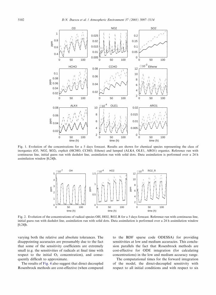
Fig. 1. Evolution of the concentrations for a 5 days forecast. Results are shown for chemical species representing the class of

inorganics (O3, NO2, SO2), explicit (HCHO, CCHO, Ethene) and lumped (ALK4, OLE1, ARO1) organics. Reference run with

continuous line, initial guess run with dashdot line, assimilation run with solid dots. Data assimilation is performed over a 24 h

assimilation window [0,24]h.

0 50 1000

1

2

3

4

5× 10-7 OH

ppm

time (h)0 50 100

0

0.5

1

1.5× 10-4

ppm

time (h)

HO2

0 50 100

2

4

6

8

10

12× 10-5

ppm

time (h)

RO2_R

Fig. 2. Evolution of the concentrations of radical species OH, HO2, RO2 R for a 5 days forecast. Reference run with continuous line,

initial guess run with dashdot line, assimilation run with solid dots. Data assimilation is performed over a 24 h assimilation window

[0,24]h.


varying both the relative and absolute tolerances. The

disappointing accuracies are presumably due to the fact

that some of the sensitivity coefficients are extremely

small (e.g. the sensitivities of radicals at final time with

respect to the initial O3 concentration), and conse-

quently difficult to approximate.

The results of Fig. 4 also suggest that direct decoupled

Rosenbrock methods are cost-effective (when compared

to the BDF sparse code ODESSA) for providing

sensitivities at low and medium accuracies. This conclu-

sion parallels the fact that Rosenbrock methods are

cost-effective for ODE integration (for calculating

concentrations) in the low and medium accuracy range.

The computational times for the forward integration

of the model, the direct-decoupled sensitivity with

respect to all initial conditions and with respect to six

ARTICLE IN PRESS

Table 3

The CPU times (in seconds, on a Pentium III, 1 GHz) for the

integration of the forward model, and the integration of the

direct-decoupled system for sensitivities with respect to all

initial values and with respect to six rate coefficients. Variable

integration time stepping is employed. In parentheses are shown

the ratios of DDM times to model integration times

Method Model DDM init. cond. DDM rate coeff.

ðNVAR ¼ 74Þ ðNCOEFF ¼ 6Þ

Ros2 1.87 73.60 (40) 11.01 (6)

Rodas3 0.66 25.54 (39) 10.36 (15)

Ros4 1.28 78.50 (61) 11.12 (9)

Odessa 2.23 87.82 (40) 21.57 (10)

2 5 10 20 50 10010

-10

10-8

10-6

10-4

10-2

100

Rel

ativ

e E

rror

CPU time [sec.]

O3(tF)

2 5 10 20 50 10010-10

10-8

10-6

10-4

10-2

100

CPU time [sec.]

∂ y(tF) / ∂ O3(t0)

Ros2Ros4Rodas3Odessa

2 5 10 20 50 10010-10

10-8

10-6

10-4

10-2

100

CPU time [sec.]

∂ O3(tF) / ∂ y(t0)

Fig. 4. The numerical errors versus CPU time for: ½O3�ðtFÞ (left), the direct sensitivity @yðtFÞ=@½O3�ðt0Þ (middle), and the direct

sensitivity @½O3�ðtFÞ=@yðt0Þ (right).

0 20 40 60 80 100 120-20

-15

-10

-5

0

5

Time [hours]

k2

O3P + O2 → O3

0 20 40 60 80 100 120-4

-2

0

2× 10-5

Time [hours]

k3

O3P + O3 → 2O2

0 20 40 60 80 100 1200

0.5

1

1.5

2

2.5

Time [hours]

k7

O3 + NO → NO2

0 20 40 60 80 100 120-2

-1.5

-1

-0.5

0

0.5

Time [hours]

k8

O3 + NO2 → NO3

∂

log

O3(

t) /

∂ lo

g k i

0 20 40 60 80 100 120-0.015

-0.01

-0.005

0

0.005

0.01

0.015

0.02

Time [hours]

k30

OH + O3 → HO2

0 20 40 60 80 100 120-0.15

-0.1

-0.05

0

0.05

0.1

0.15

Time [hours]

k36

HO2 + O3 → OH

∂ lo

g O

3(t)

/ ∂

log

k i

Fig. 3. The time evolution of ½O3�ðtÞ direct sensitivity with respect to several rate coefficients.


rate coefficients are shown in Table 3. The ratios of

DDM times to model integration times are sub-linear

(about half the number of sensitivity coefficients) for

sensitivity with respect to initial values. But these ratios

are super-linear for the sensitivities with respect to rate

coefficients. This can be explained by the overheads due

to the analytical calculation of the function and

Jacobian derivatives with respect to the rate coefficients.

4. Adjoint sensitivity analysis

In this section, we use the adjoint method to estimate

the sensitivity of predicted ozone concentration ½O3�ðtFÞ


at tF ¼ t0 þ 120h; first with respect to the initial

conditions y0; then with respect to the model state at

intermediate instants in time t0ptotF; emissions and

reaction rate coefficients. Issues related with validation

of the model linearization, consistency between the

discrete adjoint (DADJ) and continuous adjoint (CADJ)

model, and accuracy of the evaluated gradients are

addressed. A comparative study discrete versus contin-

uous adjoint is presented. The computational expense of

the adjoint model is analyzed in terms of memory

storage requirements and CPU time relative to the

forward model integration.

4.1. Adjoint model validation

The direct and the adjoint sensitivity methods provide

first-order sensitivities that describe the linear response

of the system with respect to variations in the model

parameters. Since chemical reaction systems are non-

linear, the first problem to address is the validity of the

linearization of model (1). For a given objective

functional

gðpÞ ¼ gðyðtF; pÞÞ ð2Þ

we will assume that the model linearization is satisfied

and the evaluated sensitivity (gradient) rgðpÞ ¼@g=@pARm is correct if the finite difference approxima-

tion

gðp þ eieiÞ � gðpÞei

E@gðpÞ@pi

; 1pipm ð3Þ

is satisfactory for ei small enough. In the equation

above, ei ¼ ð0;y; 0; 1; 0y; 0ÞTARm is the unit vector in

the ith direction of Rm:Additional issues must be addressed for the adjoint

model validation. Model (1) is nonlinear such that the

adjoint model depends on the forward state evolution,

which in turn depends on the parameter values. When

variable step size integration is performed, the selected

steps depend on the parameter values. For a valid test

(3) there are two alternatives:

(i)
perform a constant step size integration;
(ii)
perform a variable step size integration to evaluate
gðpÞ and store the sequence of the steps taken. Then

evaluate gðp þ eieiÞ using the same sequence of steps.

Using either (i) or (ii) we may perform a valid test for the

discrete adjoint model which provides the sensitivity of

the numerically evaluated response functional with

respect to the model parameters. Since the forward

model provides only approximate values of the con-

tinuum trajectory, the test (3) for the continuous adjoint

gradients can only lead to an agreement within OðeÞ þOðTolÞ; where Tol represents the accuracy of the

forward integration. We use a constant step size

integration to validate the discrete adjoint model, then

we show the consistency between the discrete and

continuous adjoint models for an accurate variable step

size forward/adjoint model integration.

4.1.1. Discrete adjoint model validation

We consider the ozone concentration at tF ¼ t0 þ120h as the response functional, and the initial condi-

tions as parameters. Therefore, p ¼ y0 and gðy0Þ ¼½O3�ðtF; y0Þ: Sensitivities are evaluated for a constant

step size integration h ¼ 60 s using ROS2 and RODAS3

solvers. For each solver we compare the discrete adjoint

sensitivity against the finite difference approximation

(3). Due to the wide range of concentrations, non-

linearity of the system and roundoff errors, finding an

optimal perturbation e for the finite difference approx-

imation may be a difficult task requiring extensive trial

and error experiments. We consider a perturbation in

the initial conditions of 1 part-per-trillion (ppt) for each

chemical species at a time, and perform 1 þ 74 runs for

the finite difference approximation. For most of the

chemical species an agreement of 4–6 significant digits is

observed between the finite difference and the discrete

adjoint gradients, which indicates that the adjoint

gradients are properly evaluated. Sensitivity values using

finite difference (FD) against discrete adjoint (DADJ)

are presented in Table 1 for all chemical species and each

numerical solver. In addition, the sensitivities obtained

with the continuous adjoint model (CADJ) are also

included in Table 1 for each solver. Note that the first

eight chemical species in Table 1 are non-reactive and

therefore their sensitivity values are zero. For some of

the radical species (marked with � in Table 1), we used a

perturbation of 10�3 ppt to obtain a satisfactory finite

difference approximation. Only for the phenoxy radical

(BZNO2 O) the finite difference approximation failed to

provide reliable results. Since in our model the

concentration of BZNO2 O is about 10�16 ppt; roundoff

errors play a significant role in the finite difference

estimate.

From Table 1 it can be seen that although in general

we obtained close sensitivity values with different

integrators, the accuracy of the forward integration

may have a significant impact on the evaluated

sensitivities. A good agreement between the finite

difference approximation and the discrete adjoint

evaluated sensitivities simply implies that the adjoint

model was properly implemented. No indication is

provided on how accurately we estimated the true

sensitivities given by the exact solution of the forward/

adjoint model. For some of the radical species and in

particular, for the hydroxyl radical (OH) the discrete

adjoint sensitivities we obtained with ROS2 and

RODAS3 are quite different. These results indicate that

the errors in computing the state evolution may be

amplified through the differentiation of the numerical

schemes. On another hand, the continuous adjoint

ARTICLE IN PRESSD.N. Daescu et al. / Atmospheric Environment 37 (2003) 5097–5114 5105

method applied for each solver offered a consistent

sensitivity estimate and we obtained an accurate

sensitivity value @½O3�ðtFÞ=@½OH�ðt0Þ ¼ 0:003891 with

ODESSA package (see also Section 4.2) using the direct

decoupled sensitivity method.

4.2. Accuracy of the adjoint sensitivities

We investigated the accuracy of the sensitivities

evaluated with the continuous and discrete adjoint

models. Reference sensitivity values were obtained by

solving the ODE system (1) and the associated first-

order parametric sensitivity equations using ODESSA

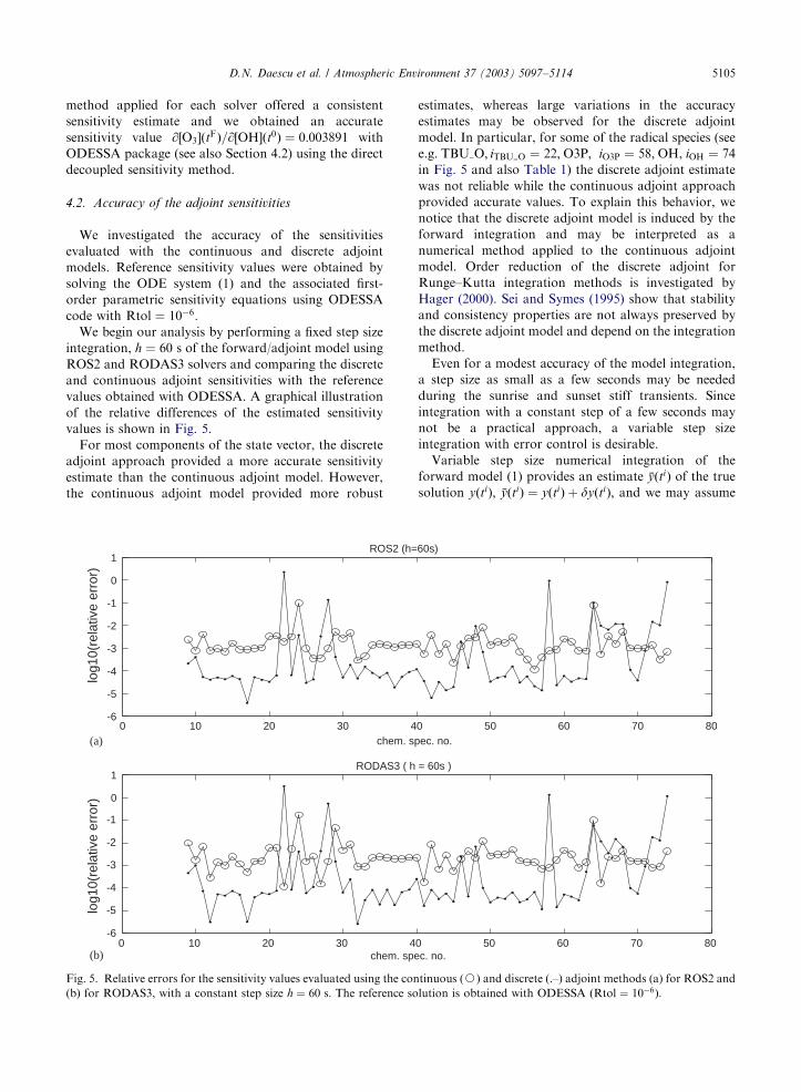
code with Rtol ¼ 10�6:We begin our analysis by performing a fixed step size

integration, h ¼ 60 s of the forward/adjoint model using

ROS2 and RODAS3 solvers and comparing the discrete

and continuous adjoint sensitivities with the reference

values obtained with ODESSA. A graphical illustration

of the relative differences of the estimated sensitivity

values is shown in Fig. 5.

For most components of the state vector, the discrete

adjoint approach provided a more accurate sensitivity

estimate than the continuous adjoint model. However,

the continuous adjoint model provided more robust

0 10 20 30 4-6

-5

-4

-3

-2

-1

0

1ROS2 (h=

chem. s

log1

0(re

lativ

e er

ror)

0 10 20 30 4-6

-5

-4

-3

-2

-1

0

1

chem. spe

log1

0(re

lativ

e er

ror)

RODAS3 ( h

(a)

(b)

Fig. 5. Relative errors for the sensitivity values evaluated using the con

(b) for RODAS3, with a constant step size h ¼ 60 s: The reference so

estimates, whereas large variations in the accuracy

estimates may be observed for the discrete adjoint

model. In particular, for some of the radical species (see

e.g. TBU O; iTBU O ¼ 22; O3P; iO3P ¼ 58; OH, iOH ¼ 74

in Fig. 5 and also Table 1) the discrete adjoint estimate

was not reliable while the continuous adjoint approach

provided accurate values. To explain this behavior, we

notice that the discrete adjoint model is induced by the

forward integration and may be interpreted as a

numerical method applied to the continuous adjoint

model. Order reduction of the discrete adjoint for

Runge–Kutta integration methods is investigated by

Hager (2000). Sei and Symes (1995) show that stability

and consistency properties are not always preserved by

the discrete adjoint model and depend on the integration

method.

Even for a modest accuracy of the model integration,

a step size as small as a few seconds may be needed

during the sunrise and sunset stiff transients. Since

integration with a constant step of a few seconds may

not be a practical approach, a variable step size

integration with error control is desirable.

Variable step size numerical integration of the

forward model (1) provides an estimate %yðtiÞ of the true

solution yðtiÞ; %yðtiÞ ¼ yðtiÞ þ dyðtiÞ; and we may assume

0 50 60 70 80

60s)

pec. no.

0 50 60 70 80c. no.

= 60s )

tinuous (J) and discrete (.–) adjoint methods (a) for ROS2 and

lution is obtained with ODESSA ðRtol ¼ 10�6Þ:


that the accuracy requirements of the forward integra-

tion are such that jjdyðtiÞjjoTol; where Tol is an user

prescribed tolerance.

In the continuous adjoint approach we only have

access to the approximate adjoint model

dldt

¼ �JT ðt; %y; pÞl; ð4Þ

lðtFÞ ¼@g

@yð %yðtFÞÞ; ð5Þ

which we attempt to solve numerically. If a forward

model solution %yðtiÞ such that jjdyðtiÞjjoTol is provided,

by solving Eqs. (4)–(5) we may only obtain an estimate%l ¼ lþ dl with jjdljjoC Tol and the constant bound

may be quite large. A judicious estimate of how the

forward integration errors propagate into the adjoint

model is difficult to obtain and significant insight may be

gained through a second-order sensitivity analysis to

evaluate @l=@y: Such analysis is beyond the goal of this

paper and we will consider a backward integration of the

adjoint model (4)–(5) using the reversed sequence of

steps taken during the forward integration.

The forward model (1) is integrated as in Section 2.1

with the tolerances Atol ¼ 1 mol=cm3; Rtol ¼ 10�3;using the variable step size ROS2 and RODAS3 solvers

and reference sensitivity values are obtained with

ODESSA.

0 10 20 30 4-0.4

-0.3

-0.2

-0.1

0

0.1

0.2

0.3

0.4

∂ O

3(tF

)/∂

y i(t0 )

chem.

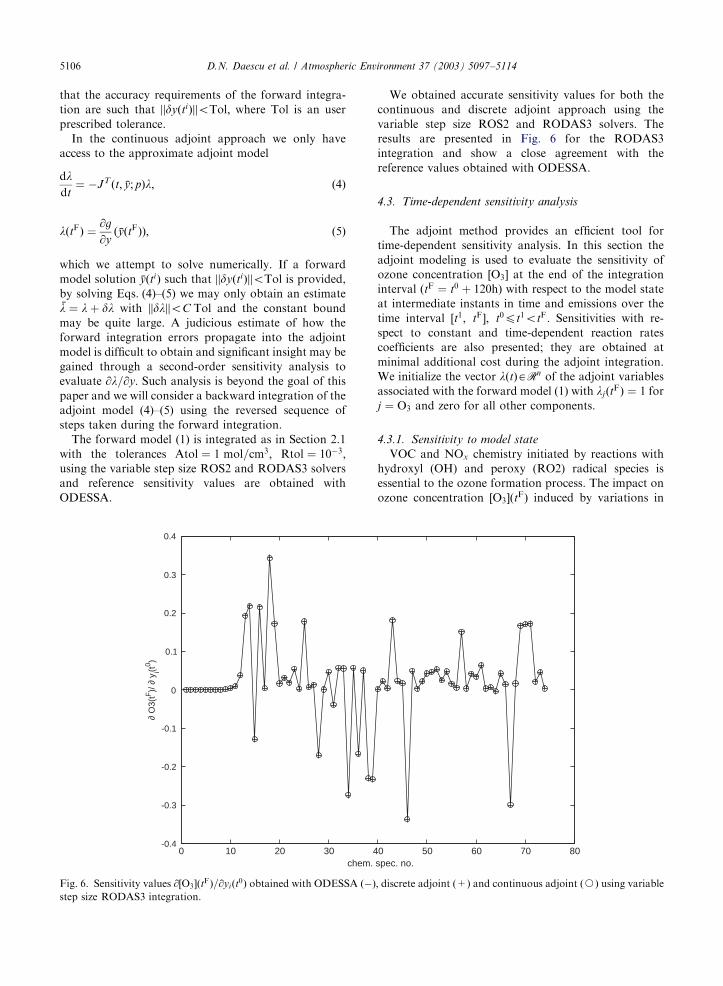
Fig. 6. Sensitivity values @½O3�ðtFÞ=@yiðt0Þ obtained with ODESSA ð�Þstep size RODAS3 integration.

We obtained accurate sensitivity values for both the

continuous and discrete adjoint approach using the

variable step size ROS2 and RODAS3 solvers. The

results are presented in Fig. 6 for the RODAS3

integration and show a close agreement with the

reference values obtained with ODESSA.

4.3. Time-dependent sensitivity analysis

The adjoint method provides an efficient tool for

time-dependent sensitivity analysis. In this section the

adjoint modeling is used to evaluate the sensitivity of

ozone concentration ½O3� at the end of the integration

interval ðtF ¼ t0 þ 120hÞ with respect to the model state

at intermediate instants in time and emissions over the

time interval ½t1; tF�; t0pt1otF: Sensitivities with re-

spect to constant and time-dependent reaction rates

coefficients are also presented; they are obtained at

minimal additional cost during the adjoint integration.

We initialize the vector lðtÞARn of the adjoint variables

associated with the forward model (1) with ljðtFÞ ¼ 1 for

j ¼ O3 and zero for all other components.

4.3.1. Sensitivity to model state

VOC and NOx chemistry initiated by reactions with

hydroxyl (OH) and peroxy (RO2) radical species is

essential to the ozone formation process. The impact on

ozone concentration ½O3�ðtFÞ induced by variations in

0 50 60 70 80spec. no.

; discrete adjoint (+) and continuous adjoint ðJÞ using variable


the concentrations of the chemical species in the model

at intermediate instants in time t0ptotF may be

analyzed by evaluating the time-dependent sensitivities

siðtÞ ¼@½O3�ðtFÞ@yiðtÞ

; 1pipn: ð6Þ

Using the adjoint model properties (Sandu et al., 2003),

we identify siðtÞ ¼ liðtÞ such that during the adjoint

integration to obtain sensitivity with respect to the initial

state lðt0Þ; we obtain at no additional cost the

intermediate sensitivities (6). Due to the wide range of

concentrations in the chemical system, we consider

normalized sensitivity values given by the ratio

s�i ðtÞ ¼@½O3�ðtFÞ@yiðtÞ

yiðtÞ½O3�ðtFÞ

¼yiðtÞ

½O3�ðtFÞliðtÞ; 1pipn; ð7Þ

which may be interpreted as the percentual change in the

concentration ½O3�ðtFÞ due to 1% increase in the

concentration of species i at moment t:The adjoint integration provided the sensitivities of

ozone with respect to all chemical species in the model

and we obtained consistent estimates of s�i ðtÞ; t0ptotF

0 20 40 60 80 100 120

-20

-15

-10

-5

0

time (h)

HCHOCCHORCHO

0 20 40 60 80 100 1200

0.01

0.02

0.03

0.04

0.05

time (h)

∂ [O

3] (

tF)

/ ∂ y

i (t)

(%

/%)

NO2NO*10

× 10-3

∂ [O

3] (

tF)

/ ∂ y

i (t)

(%

/%)

Fig. 7. Normalized ½O3�ðtFÞ sensitivity with respect to concentrations o

radicals OH and HO2 (bottom) at time t; t0ptptF:

within the prescribed accuracy range for both contin-

uous and discrete adjoint approach using a variable step

size integration.

Ozone formation is highly sensitive to the concentra-

tions of NOx species, as shown in Fig. 7. Increasing NO

and NO2 concentrations result in increased ozone

formation and the relative impact is highly dependent

on the time of the day. Small relative sensitivities were

obtained with respect to the radical species OH and

HO2. Among the explicit reactive organic product

species we found that the impact of variations in the

formaldehyde (HCHO) and acetaldehyde (CCHO)

concentrations were significant for the short time

evolution of ozone concentrations. Among the lumped

parameter species, a large relative sensitivity was

obtained for lumped aldehydes (RCHO), alkanes with

high OH reactivity (ALK4, ALK5), and aromatics

(ARO1, ARO2). These results are also displayed in

Fig. 7.

As a general remark, we notice that the sensitivity of

ozone concentration at the end of the integration

interval with respect to the state configuration during

the previous 24 h is relatively large and it rapidly

diminishes as time moves backward. Therefore, small

0 20 40 60 80 100 120

-10

-5

0

5

time (h)

ALK4ALK5ARO1ARO2

∂ [O

3] (

tF)

/ ∂ y

i (t)

(%

/%)

0 20 40 60 80 100 120

-15

-10

-5

0

× 10-6

time (h)

HO2OH*100

× 10-3

∂ [O

3] (

tF)

/ ∂ y

i (t)

(%

/%)

f several explicit and lumped organic species (top), NOx; and the


variations in the concentrations during the first three

days of the integration will have little influence on the

ozone state at the end of the fifth day.

4.3.2. Sensitivity to emissions

The impact of various types of emitted VOC on ozone

formation is given by the ozone reactivities of the VOC.

The ‘‘incremental reactivity’’ (Carter, 1994) is given by

the partial derivative of ozone with respect to the

emissions of the VOC which represents the sensitivity of

ozone to VOCs emissions. In this section we study the

sensitivity of ozone concentration ½O3� at the end of the

integration interval ðtF ¼ t0 þ 120hÞ with respect to NOx

and VOCs emissions over the time interval

½t1; tF�; t0pt1otF: In our model emissions are specified

for 30 chemical species at a constant rate Ei as shown in

Table 2 ðErefi Þ such that the total amount of pollutant i

emitted in the time interval ½t1; tF� is given by

Eiðt1Þ ¼Z tF

t1EiðtÞ dt ¼ ðtF � t1ÞEi: ð8Þ

The sensitivities

siðE; t1Þ ¼@½O3�ðtFÞ@Eiðt1Þ

¼1

tF � t1

Z tF

t1liðtÞ dt ð9Þ

may be evaluated simultaneously for all emission types

using a single backward integration of the adjoint model.

To derive Eq. (9) we used @fj=@Ei ¼ 1 if i ¼ j; @fj=@Ei ¼ 0

if iaj and the results in Section 3.1 in the companion

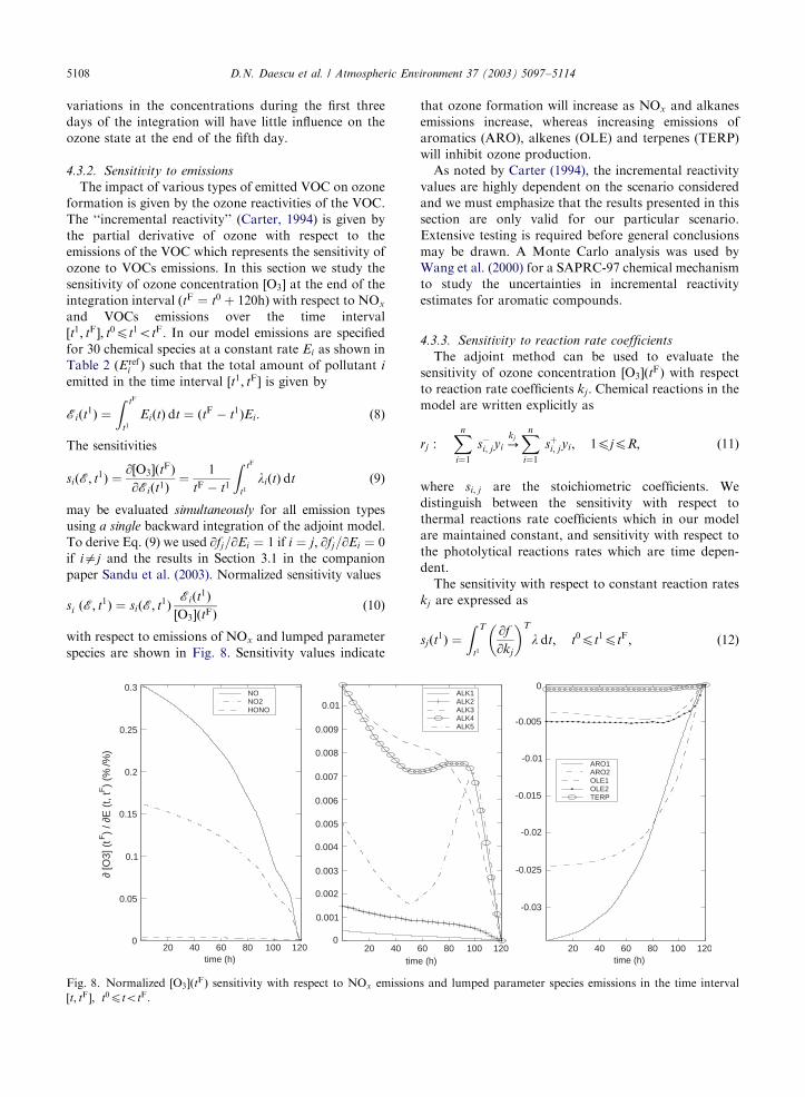
paper Sandu et al. (2003). Normalized sensitivity values

s�i ðE; t1Þ ¼ siðE; t1Þ

Eiðt1Þ½O3�ðtFÞ

ð10Þ

with respect to emissions of NOx and lumped parameter

species are shown in Fig. 8. Sensitivity values indicate

20 40 60 80 100 1200

0.05

0.1

0.15

0.2

0.25

0.3

time (h)

∂ [O

3] (

tF)

/ ∂E

(t,

tF)

(%/%

)

NONO2HONO

20 400

0.001

0.002

0.003

0.004

0.005

0.006

0.007

0.008

0.009

0.01

tim

Fig. 8. Normalized ½O3�ðtFÞ sensitivity with respect to NOx emission

½t; tF�; t0ptotF:

that ozone formation will increase as NOx and alkanes

emissions increase, whereas increasing emissions of

aromatics (ARO), alkenes (OLE) and terpenes (TERP)

will inhibit ozone production.

As noted by Carter (1994), the incremental reactivity

values are highly dependent on the scenario considered

and we must emphasize that the results presented in this

section are only valid for our particular scenario.

Extensive testing is required before general conclusions

may be drawn. A Monte Carlo analysis was used by

Wang et al. (2000) for a SAPRC-97 chemical mechanism

to study the uncertainties in incremental reactivity

estimates for aromatic compounds.

4.3.3. Sensitivity to reaction rate coefficients

The adjoint method can be used to evaluate the

sensitivity of ozone concentration ½O3�ðtFÞ with respect

to reaction rate coefficients kj : Chemical reactions in the

model are written explicitly as

rj :Xn

i¼1

s�i; jyi !kjXn

i¼1

sþi; jyi; 1pjpR; ð11Þ

where si; j are the stoichiometric coefficients. We

distinguish between the sensitivity with respect to

thermal reactions rate coefficients which in our model

are maintained constant, and sensitivity with respect to

the photolytical reactions rates which are time depen-

dent.

The sensitivity with respect to constant reaction rates

kj are expressed as

sjðt1Þ ¼Z T

t1

@f

@kj

� �T

l dt; t0pt1ptF; ð12Þ

60 80 100 120e (h)

ALK1ALK2ALK3ALK4ALK5

20 40 60 80 100 120

-0.03

-0.025

-0.02

-0.015

-0.01

-0.005

0

time (h)

ARO1ARO2OLE1OLE2TERP

s and lumped parameter species emissions in the time interval


where

@fi

@kj

¼ ðsþi; j � s�i; jÞYn

i¼1

ys�i; j

i ð13Þ

and l is the vector of adjoint variables associated with

the state vector y: We used the trapezoidal rule to

evaluate the right-hand side integrals in Eq. (12) and

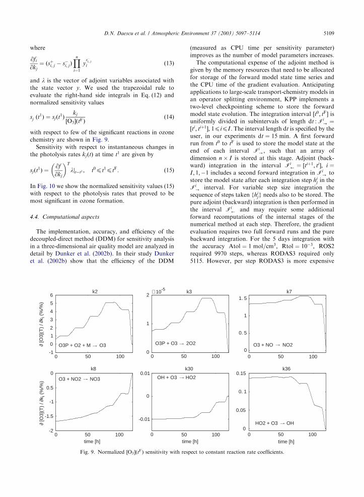
normalized sensitivity values

s�j ðt1Þ ¼ sjðt1Þ

kj

½O3�ðtFÞð14Þ

with respect to few of the significant reactions in ozone

chemistry are shown in Fig. 9.

Sensitivity with respect to instantaneous changes in

the photolysis rates kjðtÞ at time t1 are given by

sjðt1Þ ¼@f

@kj

� �T

ljt¼t1 ; t0pt1ptF: ð15Þ

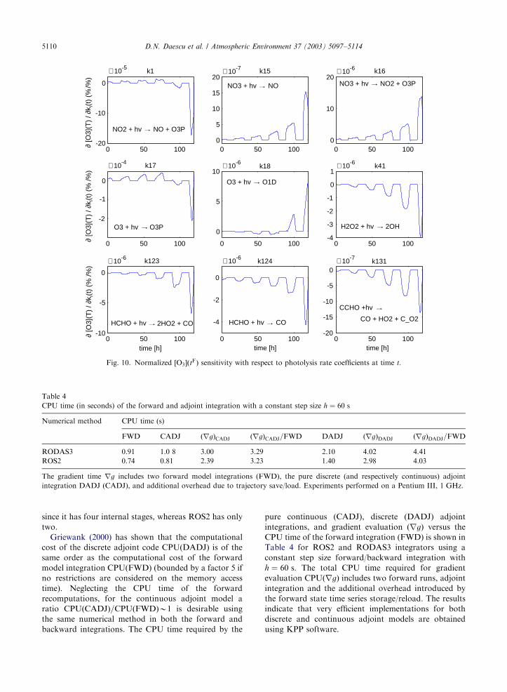
In Fig. 10 we show the normalized sensitivity values (15)

with respect to the photolysis rates that proved to be

most significant in ozone formation.

4.4. Computational aspects

The implementation, accuracy, and efficiency of the

decoupled-direct method (DDM) for sensitivity analysis

in a three-dimensional air quality model are analyzed in

detail by Dunker et al. (2002b). In their study Dunker

et al. (2002b) show that the efficiency of the DDM

0 50 100-1

0

1

2

3

4

5

6k2

O3P + O2 + M O3

0 500

1

2× 10-5 k

O3P + O3 2

0 50 100-2

-1.5

-1

0.5

0k8

O3 + NO2 NO3

time [h] tim

∂ [O

3](T

) / ∂

k i (

%/%

)

0 50

-0.01

0

0.01k3

OH + O3 H

→ →

→→

∂ [O

3](T

) / ∂

k i (

%/%

)

Fig. 9. Normalized ½O3�ðtFÞ sensitivity with resp

(measured as CPU time per sensitivity parameter)

improves as the number of model parameters increases.

The computational expense of the adjoint method is

given by the memory resources that need to be allocated

for storage of the forward model state time series and

the CPU time of the gradient evaluation. Anticipating

applications to large-scale transport-chemistry models in

an operator splitting environment, KPP implements a

two-level checkpointing scheme to store the forward

model state evolution. The integration interval ½t0; tF� is

uniformly divided in subintervals of length dt :Ii- ¼

½ti; tiþ1�; 1pipI : The interval length dt is specified by the

user, in our experiments dt ¼ 15 min: A first forward

run from t0 to tF is used to store the model state at the

end of each interval Ii-; such that an array of

dimension n � I is stored at this stage. Adjoint (back-

ward) integration in the interval Ii’ ¼ ½tiþ1; ti�; i ¼

I ; 1;�1 includes a second forward integration in Ii- to

store the model state after each integration step hij in the

Ii- interval. For variable step size integration the

sequence of steps taken fhijg needs also to be stored. The

pure adjoint (backward) integration is then performed in

the interval Ii’ and may require some additional

forward recomputations of the internal stages of the

numerical method at each step. Therefore, the gradient

evaluation requires two full forward runs and the pure

backward integration. For the 5 days integration with

the accuracy Atol ¼ 1 mol=cm3; Rtol ¼ 10�3; ROS2

required 9970 steps, whereas RODAS3 required only

5115. However, per step RODAS3 is more expensive

100

3

O2

0 50 1000

0. 5

1

1. 5k7

O3 + NO NO2

e [h]100

0

O2

0 50 1000

0.05

0. 1

0.15k36

HO2 + O3 OH

time [h]

→

→

ect to constant reaction rate coefficients.

ARTICLE IN PRESS

0 50 100-20

-10

0

k1

NO2 + hv NO + O3P

0 50 1000

5

10

15

20k15

NO3 + hv NO

0 50 1000

10

20k16

NO3 + hv NO2 + O3P

0 50 100

-2

-1

0

k17

O3 + hv O3P

0 50 100

0

5

10k18

O3 + hv O1D

0 50 100-4

-3

-2

-1

0

1k41

H2O2 + hv 2OH

0 50 100-10

-5

0

× 10-6 k123

HCHO + hv 2HO2 + CO

time [h]

∂ [O

3](T

) / ∂

k i(t

) (%

/%)

∂ [O

3](T

) / ∂

k i(t

) (%

/%)

∂ [O

3](T

) / ∂

k i(t

) (%

/%)

0 50 100

-4

-2

0

k124

HCHO + hv →

→

→

→

→

→

→

CO

time [h]0 50 100

-20

-15

-10

-5

0k131

CCHO +hv

CO + HO2 + C_O2

time [h]

× 10-6 × 10-7

× 10-6× 10-6× 10-4

× 10-5 × 10-7 × 10-6

→→

Fig. 10. Normalized ½O3�ðtFÞ sensitivity with respect to photolysis rate coefficients at time t:

Table 4

CPU time (in seconds) of the forward and adjoint integration with a constant step size h ¼ 60 s

Numerical method CPU time (s)

FWD CADJ ðrgÞCADJ ðrgÞCADJ=FWD DADJ ðrgÞDADJ ðrgÞDADJ=FWD

RODAS3 0.91 1.0 8 3.00 3.29 2.10 4.02 4.41

ROS2 0.74 0.81 2.39 3.23 1.40 2.98 4.03

The gradient time rg includes two forward model integrations (FWD), the pure discrete (and respectively continuous) adjoint

integration DADJ (CADJ), and additional overhead due to trajectory save/load. Experiments performed on a Pentium III, 1 GHz:


since it has four internal stages, whereas ROS2 has only

two.

Griewank (2000) has shown that the computational

cost of the discrete adjoint code CPU(DADJ) is of the

same order as the computational cost of the forward

model integration CPU(FWD) (bounded by a factor 5 if

no restrictions are considered on the memory access

time). Neglecting the CPU time of the forward

recomputations, for the continuous adjoint model a

ratio CPUðCADJÞ=CPUðFWDÞB1 is desirable using

the same numerical method in both the forward and

backward integrations. The CPU time required by the

pure continuous (CADJ), discrete (DADJ) adjoint

integrations, and gradient evaluation ðrgÞ versus the

CPU time of the forward integration (FWD) is shown in

Table 4 for ROS2 and RODAS3 integrators using a

constant step size forward/backward integration with

h ¼ 60 s: The total CPU time required for gradient

evaluation CPUðrgÞ includes two forward runs, adjoint

integration and the additional overhead introduced by

the forward state time series storage/reload. The results

indicate that very efficient implementations for both

discrete and continuous adjoint models are obtained

using KPP software.


4.4.1. On the applicability of the direct and adjoint

sensitivity methods

The integration of the direct and adjoint sensitivity

models provides complementary information. In the

direct approach, the sensitivities of all concentrations

with respect to one parameter, e.g. @yðtFÞ=@yjðt0Þ; may be

obtained by integrating one additional n-dimensional

sensitivity equation. During this integration the deriva-

tives @yðtÞ=@yjðt0Þ; t0ototF of the time-varying concen-

trations are also obtained at no additional cost. In the

adjoint approach, the sensitivity of an objective func-

tional with respect to all model parameters, e.g.

@O3ðtFÞ=@yðt0Þ; may be obtained using a single computa-

tional run of the n-dimensional adjoint model. During

this integration, the derivatives with respect to the time

varying concentrations @O3ðtFÞ=@yðtÞ; t0ototF are also

obtained at no additional cost.

In the direct sensitivity approach the computational

cost increases with the number of parameters, whereas in

the adjoint approach the computational cost increases

with the number of objective functionals. From this

point of view, the adjoint method is particularly suitable

for large-scale variational data assimilation applications

where the sensitivity (gradient) of a scalar cost

functional must be computed. The results presented in

Tables 3 and 4 provide insight on the efficiency of the

direct and adjoint methods for gradient evaluation. One

should notice that while the results for the direct-

decoupled method are presented for a variable step size

integration, the results for the adjoint method are

presented for a constant step size ðh ¼ 60 sÞ integration.

Therefore, the absolute CPU time does not provide a

valid measure for comparison. As a measure of

efficiency, we consider the ratio between the CPU time

to obtain the sensitivities and the CPU time of the

forward model integration. While the ratios obtained

with the direct-decoupled method range from 39 to 61,

the adjoint method provided the gradient at a ratio

between 3 (continuous adjoint) and 4.5 (discrete

adjoint). These results show that the adjoint modeling

is a more efficient approach to evaluate the sensitivity of

a scalar response function with respect to a large number

of input parameters.

Seefeld and Stockwell (1999) showed how the

decoupled direct method (DDM) may be used to

provide sensitivities with respect to time dependent

parameters. For comprehensive three-dimensional air

quality models, the DDM has been successfully applied

by Dunker et al. (2002a, b) to obtain sensitivities of the

model output with respect to a relatively small number

of parameters ðB102Þ: Dominguez and Russell (2000)

use DDM to perform a four-dimensional data assimila-

tion for emissions estimates. The adjoint method has

been proved to be a feasible tool for large-scale (B106

parameters) chemical data assimilation (Elbern and

Schmidt, 1999; Errera and Fonteyn, 2001).

5. Applications to variational data assimilation

Adjoint modeling is an essential tool for large-scale

variational data assimilation applications. The varia-

tional methods have been extensively used in data

assimilation for meteorological and oceanographical

models and show promising results for atmospheric

chemistry applications (Fisher and Lary, 1995; Elbern

and Schmidt, 1999; Errera and Fonteyn, 2001). Four-

dimensional variational data assimilation (4D-Var)

searches for an optimal set of model parameters which

minimizes the discrepancies between the model forecast

and time distributed observational data over the

assimilation window. A practical implementation of

the minimization process requires a fast and accurate

evaluation of the gradient of the cost functional which

may be provided by adjoint modeling.

In meteorological applications variational techniques

are mostly used to find an optimal initial state of the

model ðp ¼ y0Þ: In atmospheric chemistry modeling

uncertainties in various model input parameters (e.g.

emission rates, boundary values) must be also consid-

ered. For an in-depth analysis of the parameter

estimation, identifiability issues and regularization

techniques in the context of inverse modeling we will

refer to Tarantola (1987). A review of the use of the

adjoint method in four-dimensional atmospheric chem-

istry data assimilation is presented by Wang et al.

(2001). In this section we investigate the ability of the

4D-Var technique to retrieve the initial model state and

provide accurate emission estimates using observational

data information. We briefly outline a discrete 4D-Var

problem formulation and we will refer to Jazwinski

(1970) and Daley (1991) for a complete description of

the various assumptions used by the data assimilation

techniques and the probabilistic interpretation. The

numerical experiments are performed using the ROS2

solver with variable step size and a discrete adjoint

model.

5.1. Data assimilation framework

The data assimilation procedure is set using the twin

experiments method as follows:

Reference run: we start a model run at local noon

ts ¼ 12:00LT with the concentration of all variable

chemical species set to zero and the ‘‘reference’’ emission

rates Erefi shown in Table 2. The model state obtained

after a 24 h run at t0 ¼ ts þ 24h is considered as

reference (‘‘true’’) initial state ðy0Þref of the model for a

5 days reference run ½t0; t0 þ 120h�:Initial guess run: the experiment is repeated with

emission rates increased by 50%, Eiguessi ¼ 1:5Eref

i ; as

shown in Table 2. The model state obtained after a 24 h

run at t0 ¼ ts þ 24h is considered as ‘‘initial guess’’


model state for a 5 days forecast run using Eiguessi as

emission rates.

Observations and assimilation window: We consider a

24 h assimilation window ½t0; t0 þ 24h�: No observations

are provided for radical species (marked with } in

Table 1). For all other chemical species in the model

concentrations obtained during the reference run are

provided as hourly observations %yki starting from t0 þ

1h:Parameters: the control parameters are the concentra-

tion of variable chemical species at t0 (dimension 74) and

the emission rates (dimension 30), p ¼ ðy0T ;ET ÞT :Cost functional: We assume that information to the

data assimilation process is provided only by the

‘‘observations’’ such that no background term is

included in the cost functional. To achieve a better

scaling and to eliminate the positivity constraint, we

consider ln p as control variables and the logarithmic

form of the cost functional

Jðln pÞ ¼1

2

X24

k¼1

XiAOk

½ln yki � ln %y

ki �

2; ð16Þ

where Ok represents the set of components of the state

vector observed at tk:Optimization algorithm: Quasi-Newton limited mem-

ory L-BFGS (Byrd et al., 1995). The optimization

proceeds until the cost functional is reduced to 0.01% of

its initial value.

5.2. Numerical results

Using data assimilation we aim to provide an accurate

estimate of the true initial model state ðy0Þref and

emission rates Erefi such that an improved forecast is

obtained for a 5 days model run. In the data assimilation

process information provided by the observations is

propagated to all the variables of the model. Chemical

interactions among the model variables may allow the

assimilation process to provide an improved forecast not

only for the observed components of the state vector,

but also for the chemical species for which observations

are not available. Therefore, we further investigate the

ability of the data assimilation to provide an accurate

estimate of the evolution of the concentrations of radical

species for which no observations were provided.

The reference run, the initial guess forecast, the

assimilation results and the forecast after the assimila-

tion process takes place are shown in Figs. 1 and 2 for

various chemical species. By performing data assimila-

tion, not only we have obtained an accurate representa-

tion of the model state evolution in the assimilation

window [0,24]h, but also an accurate forecast was

obtained for the full five days period. An accurate

evolution of the concentrations of the radical species

was also obtained. Emission rates estimates Eassimi

displayed in Table 2 show that using data assimilation

the true emission rate values were successfully retrieved.

We notice that not all parameters were estimated with

the same accuracy (see e.g., TERP and Isoprene vs.

CCHO and MGLY) which shows that the assimilation

procedure would benefit from a better scaling (weight-

ing) of the cost functional components. Dominguez and

Russell (2000) analyzed the impact of several weighting

schemes in four-dimensional data assimilation to adjust

emissions inventories to observational data.

6. Conclusions and future work

In this paper, we presented an extensive set of

numerical experiments and applications of the new

Kinetic PreProcessor release KPP-1.2 to direct de-

coupled and adjoint sensitivity analysis. Our results

indicate that KPP may be used as a flexible and efficient

tool to generate code for sensitivity studies of the

chemical reactions mechanisms. We illustrated KPP

abilities by selecting a challenging test model, the state-

of-the-science gas-phase chemical mechanism SAPRC-

99. For this comprehensive model implementation of the

direct-decoupled sensitivity method and hand genera-

tion of the adjoint code may be a difficult, time

consuming, and error prone task.

Issues related with model linearization, accuracy,

consistency, and computational expense of the discrete

and continuous adjoint model were addressed. The new

direct-decoupled Rosenbrock methods we proposed

have been shown to be cost-effective for providing

sensitivities at low and medium accuracies. In addition,

particular properties of the Rosenbrock methods may be

exploited for the adjoint modeling (Daescu et al., 2000).

By taking full advantage of the sparsity of the chemical

mechanism, the KPP software generates efficient dis-

crete and continuous adjoint models.

Our comparative study shows that the continuous

adjoint model offers more flexibility, is computationally

less expensive, and may provide more robust results

than the discrete adjoint model. Implementation of a

discrete adjoint model is more suitable for data

assimilation applications since the provided gradient is

exact relatively to the evaluated cost functional.

We should emphasize that the efficiency of the KPP

software relies on its particular design for chemical

kinetics systems and KPP is not a general purpose

adjoint modeling tool as TAMC (Giering and Kaminski,

1998) or Odyss!ee (Rostaing et al., 1993). Generating the

discrete adjoint model associated with sophisticated

numerical integrators is a complex task and an efficient

implementation requires in-depth knowledge of the

numerical scheme and forward mode computations.

For this reason, the use of discrete adjoints in atmo-

spheric chemistry applications has been limited to


explicit or low order linearly implicit numerical meth-

ods. For efficiency, a hand generated discrete adjoint

code was often implemented (Elbern and Schmidt,

1999). Currently, KPP provides discrete adjoint imple-

mentation of the linearly implicit Euler, ROS2, and

RODAS3 solvers, whereas the continuous adjoint model

may be integrated with any user selected numerical

method. As our research advances, new solvers from the

class of Runge–Kutta methods will be included in

discrete adjoint mode.

Adjoint modeling has various applications and few of

them were illustrated in this paper: backward sensitivity

analysis, parameter estimation, and data assimilation.

Model reduction of chemical kinetics is an important

field which we will investigate in our future work using

direct/adjoint sensitivity analysis. By providing efficient

operations involving Hessian matrices, KPP software

may be also used to obtain second order information

which may be applied to sensitivity analysis and data

assimilation (Le Dimet et al., 2002).

An efficient implementation of the chemistry module

into comprehensive 3D air quality models is essential as

computations involving chemical transformations may

require as much as 90% of the total CPU time.

Applications of the adjoint method to atmospheric

chemistry represent a new research direction which is

growing at a fast pace and the KPP software may be

used to facilitate the direct/adjoint model integration.

Acknowledgements

The authors are grateful to NSF support for this work

through the award ITR AP&IM-0205198. The work of

A. Sandu was also supported in part by the NSF

CAREER award ACI-0093139. D.N. Daescu acknowl-

edges the support from the Supercomputing Institute for

Digital Simulation and Advanced Computation of the

University of Minnesota.

References

Aiken, R.C. (Ed.), 1985. Stiff Computation. Oxford University

Press, Oxford.

Byrd, R.H., Lu, P., Nocedal, J., 1995. A limited memory

algorithm for bound constrained optimization. SIAM

Journal on Scientific Computing 16 (5), 1190–1208.

Carmichael, G.R., Peters, L.K., Kitada, T., 1986. A second

generation model for regional-scale transport/chemistry/

deposition. Atmospheric Environment 20, 173–188.

Carter, W.P.L., 1994. Development of ozone reactivity scales

for volatile organic compounds. Journal of the Air and

Waste Management Association 44, 881–899.

Carter, W.P.L., 2000a. Implementation of the SAPRC-99

chemical mechanism into the models-3 framework. Report

to the United States Environmental Protection Agency,

January 2000.

Carter, W.P.L., 2000b. Documentation of the SAPRC-99

chemical mechanism for VOC reactivity assessment. Final

Report to California Air Resources Board Contract No. 92-

329, and 95-308, May 2000.

Daescu, D., Carmichael, G.R., Sandu, A., 2000. Adjoint

implementation of Rosenbrock methods applied to varia-

tional data assimilation problems. Journal of Computa-

tional Physics 165 (2), 496–510.

Daley, R., 1991. Atmospheric Data Analysis. Cambridge

University Press, Cambridge, 457pp.

Damian-Iordache, V., Sandu, A., Damian-Iordache, M.,

Carmichael, G.R., Potra, F.A., 2002. The kinetic prepro-

cessor KPP—a software environment for solving chemical

kinetics. Computers and Chemical Engineering 26 (11),

1567–1579.

Dominguez, A.M., Russell, A.G., 2000. Iterative inverse

modeling and direct sensitivity analysis of a photochemical

air quality model. Environmental Science and Technology

34, 4974–4981.

Dunker, A.M., Yarwood, G., Ortmann, J.P., Wilson, G.M.,

2002a. Comparison of source appointment and source

sensitivity of ozone in a three-dimensional air quality

model. Environmental Science and Technology 36,

2953–2964.

Dunker, A.M., Yarwood, G., Ortmann, J.P., Wilson, G.M.,

2002b. The decoupled direct method for sensitivity analysis

in a three-dimensional air quality model—implementation,

accuracy, and efficiency. Environmental Science and Tech-

nology 36, 2965–2976.

Elbern, H., Schmidt, H., 1999. A four-dimensional variational

chemistry data assimilation scheme for Eulerian chemistry

transport model. Journal of Geophysical Research 104

(D15), 18583–18598.

Errera, Q., Fonteyn, D., 2001. Four-dimensional variational

chemical assimilation of CRISTA stratospheric measure-

ments. Journal of Geophysical Research 106 (D11),

12253–12265.

Fisher, M., Lary, D.J., 1995. Lagrangian four-dimensional

variational data assimilation of chemical species. Quarterly

Journal of the Royal Meteorological Society 121, 1681–1704.

Giering, R., Kaminski, T., 1998. Recipes for adjoint code

construction. ACM Transactions on Mathematical Soft-

ware 24 (4), 437–474.

Griewank, A., 2000. Evaluating derivatives: Principles and

Techniques of Algorithmic Differentiation. Frontiers in

Applied Mathematics, Vol. 19. SIAM, Philadelphia.

Hager, W.W., 2000. Runge–Kutta methods in optimal control

and the transformed adjoint system. Numerische Mathe-

matik 87, 247–282.

Hairer, E., Wanner, G., 1991. Solving Ordinary Differential

Equations II. Stiff and Differential-Algebraic Problems.

Springer, Berlin.

Jazwinski, A.H., 1970. Stochastic Processes and Filtering

Theory. Academic Press, New York, NY.

Le Dimet, F.-X., Navon, I.M., Daescu, D.N., 2002. Second

order information in data assimilation. Monthly Weather

Review 130 (3), 629–648.

Leis, J.R., Kramer, M.A., 1986. ODESSA—an ordinary

differential equation solver with explicit simultaneous

sensitivity analysis. ACM Transactions on Mathematical

Software 14 (1), 61–67.


Lutz, A.E., Kee, R.J., Miller, J.A., 1987. SENKIN: a fortran

program for predicting homogeneous gas phase chemical

kinetics with sensitivity analysis. Sandia Report #SAND87-

8248; Sandia National Laboratories.

Radhakrishnan, K., 2003. LSENS: Multipurpose kinetics and

sensitivity analysis code for homogeneous gas-phase reac-

tions. AIAA Journal 41 (5), 848–855.

Rostaing, N., Dalmas, S., Galligo, A., 1993. Automatic

differentiation in Odyss!ee. Tellus 45, 558–568.

Sandu, A., Blom, J.G., Spee, E., Verwer, J.G., Potra, F.A.,

Carmichael, G.R., 1997. Benchmarking stiff ODE solvers

for atmospheric chemistry equations II—Rosenbrock Sol-

vers. Atmospheric Environment 31, 3459–3472.

Sandu, A., Daescu, D.N., Carmichael, G.R., 2003. Direct and

adjoint sensitivity analysis of chemical kinetic systems with

KPP: I—theory and software tools. Atmospheric Environ-

ment, this issue, doi:10.1016/j.atmosenv.2003.08.019

Seefeld, S., Stockwell, W.R., 1999. First-order sensitivity

analysis of models with time-dependent parameters: an

application to PAN and ozone. Atmospheric Environment

33, 2941–2953.

Sei, A., Symes, W.W., 1995. A note on consistency and

adjointness for numerical schemes. Technical Report 95527,

Department of Computational and Applied Mathematics,

Rice University, Houston, TX.

Tarantola, A., 1987. Inverse Problem Theory: Methods for

Data Fitting and Model Parameter Estimation. Elsevier

Science Publishers, New York, NY.

Verwer, J.G., Spee, E., Blom, J.G., Hunsdorfer, W., 1999. A

second order Rosenbrock method applied to photochemical

dispersion problems. SIAM Journal on Scientific Comput-

ing 20, 1456–1480.

Wang, L., Milford, J.B., Carter, W.P.L., 2000. Reactivity

estimates for aromatic compounds. Part 2. Uncertainty in

incremental reactivities. Atmospheric Environment 34,

4349–4360.

Wang, K.Y., Lary, D.J., Shallcross, D.E., Hall,

S.M., Pyle, J.A., 2001. A review on the use of the

adjoint method in four-dimensional atmospheric-

chemistry data assimilation. Quarterly Journal of

the Royal Meteorological Society 127 (576 (Part B))

2181–2204.

10.1016/j.atmosenv.2003.080019

direct and adjoint sensitivity analysis ofchemical...

Documents