an analysis of benefits from use of geographic information ... · an analysis of benefits from use...

AN ANALYSIS OF BENEFITS FROM USE OF GEOGRAPHIC INFORMATION SYSTEMS BY

KING COUNTY, WASHINGTON

RICHARD ZERBE AND ASSOCIATES

Gregory Babinski Dani Fumia

Travis Reynolds Pradeep Singh

Tyler Scott Richard Zerbe

March 2012

1 | P a g e

AN ANALYSIS OF BENEFITS FROM USE OF GEOGRAPHIC INFORMATION SYSTEMS BY KING COUNTY WASHINGTON1

RICHARD ZERBE AND ASSOCIATES 939 21ST AVE EAST SEATTLE WA, 98112

[email protected] Gregory Babinski

Dani Fumia Travis Reynolds Pradeep Singh Tyler Scott

Richard Zerbe

March 2012

1 This study was supported by a grant from the King County GIS Center, Seattle, Washington (partially funded by the State of Oregon), 2010-‐2011

2 | P a g e

(This Page Intentionally Left Blank)

1 | P a g e

Executive Summary1 3-‐2-‐12

AN ANALYSIS OF BENEFITS FROM USE OF GEOGRAPHIC INFORMATION SYSTEMS BY KING COUNTY WASHINGTON

Task: The analysis team of Richard Zerbe and Associates has been contracted by the King County Geographic Information Systems (GIS) Center to conduct a return on investment (ROI) study concerning the development and use of GIS within County agencies.

Methods: We utilize a with-‐and-‐without survey methodology to assess how GIS has altered agency output and effort levels, estimating benefits associated with efficiency gains (reduction in full time effort (FTEs) required to produce same level of agency output) and production capabilities (increased output relative to pre-‐GIS output level). This is compared to the annual cost to the County of funding GIS technology and implementation. We utilize a three-‐stage analysis, first interviewing various employees and agency heads to gauge the role of GIS in agency activity and the types of tasks performed using GIS. These results were then used to build an employee survey, which was administered via email to employees and managers in the various county agencies that use GIS technology. Survey respondents recorded their current production of various outputs and effort levels corresponding to these various outputs with the use of GIS technology as well as their old pre-‐GIS production and effort levels. These estimates were then compiled by output type and agency to build an aggregate estimate of agency production with and without GIS technology. These changes were then monetized using agency salary figures and FTE statistics to estimate benefits in terms of what it would cost county agencies to replicate their pre-‐GIS level of output with GIS technology (i.e. old production at new production rate), as well as what it would cost county agencies to replicate their current GIS-‐aided production level without GIS technology (i.e. new production at old production rate).

Results: We find that GIS technology appears to be an efficient, highly beneficial investment for King County. The full report presents various figures, but the most conservative estimate presented finds that the use of GIS has produced approximately $775 million in net benefits over the eighteen year period from 1992 to 2010.

Report Contents: Along with a fuller description of methods and findings, the report also speaks to the relative strengths and weaknesses of the assessment method, providing guidance for future applications. Appendices provide tables of more detailed analysis results and figures, as well as a detailed description of the survey instrument. 1 RICHARD ZERBE AND ASSOCIATES, 939 21ST AVE EAST, SEATTLE WA, 98112 Gregory Babinski, Dani Fumia, Travis Reynolds, Pradeep Singh, Tyler Scott , Richard Zerbe Contact via email at [email protected]

3 | P a g e

Table of Contents

Summary…………………………………………………………………………………………………………………...6

Survey Response Rate………………………………………………………………………………………….…….7

Methodology………………………………………………………………………………………………………….…..8

Results……………………………………………………………………………………………………………….……..10

Conclusion……………………………………………………………………………………………………….………..12

References…………………………………………………………………………………………………….…………..13

Appendices…………………………………………………………………………………………………….…………..14

A. Pertinent Survey Questions B. Cost Calculations Per Year C. Benefit Calculations at Different Labor Rates D. Benefits by Department at Different Labor Rates E. Benefits By Department F. Discussion of Anomalies in Department/Usage Calculations G. Percentage Change in Productivity and Inputs H. King County GIS Center/State of Oregon Project Team

4 | P a g e

Summary

We have been asked by a King County GIS Center (KCGIS) solicitation to perform a return on investment (ROI) study of the development and use of geographic information systems (GIS) within King County. Dr. Richard Zerbe and the Benefit-‐Cost Analysis team at Richard Zerbe and Associates implemented a multiple-‐phase methodology to assess what KCGIS got for its money. A survey questionnaire was designed based on feedback from qualitative interviews conducted in the earlier phase.

King County Washington covers an area of 2130 square miles and a population in 2010 of 1,931,000, making it the 13th most populous county in the U.S. The subject of this study is the use of GIS within King County by county agencies. King County has approximately 14,000 employees and in 2010 its annual budget was over $4 billion. The King County GIS Center with 28 professional GIS staff provides GIS services to all county agencies. Approximately 20 additional GIS professional staff work directly in county agencies. As many as 1000 county employees use GIS data and applications in their daily work.

It is clear that the use of GIS by the County has been hugely beneficial. An analysis of the survey responses indicate that overall the use of GIS – compared to not having the GIS technology -‐-‐ had a net benefit of approximately $180 million for the year 2010 alone. This estimate assumes that the quality and usefulness of GIS reports remains at the same level as pre-‐GIS. In reality, we expect that the value of GIS-‐produced outputs is almost certainly higher than comparable outputs the County produced in years prior to the implementation of GIS technology. Nevertheless, on the assumption that the marginal value of output has decreased (a linear, downward sloping demand curve) we find a lower bound estimate of net benefits of $87 million per year in 2010.2 The benefits were broken down into benefits received from: (1) cost-‐savings due to more efficient production of original output; and (2) benefits generated from increased productivity beyond the original production level.

With regards to return on investment by department in 2010, using the more conservative estimates, the Department of Natural Resources and Parks (DNRP) is estimated to benefit $87.44 million per year from having GIS technology; the Wastewater Treatment Division

2 A downward sloping demand curve assumes that there is a diminishing marginal value of output; that is, it assumes that the original outputs generated by King County prior to GIS implementation are of the highest value, since these tasks were deemed valuable even at the old, higher cost-‐per-‐output level. Theoretically, the County could have devoted more resources and achieved the same level of GIS-‐enabled output without GIS technology; the fact that this did not happen indicates that the additional outputs are likely of less value to the County. In any case, the assumption of a downward sloping demand curve simply lowers the lower-‐bound estimate of GIS benefits; if the “true” demand curve is in fact horizontal (i.e. constant marginal demand for output) or even upward-‐sloping (i.e. increasing marginal demand for output, for instance due to a synergistic effect), then the true benefit level will be even greater than estimated in this report. However, we feel it most plausible that the County at least implicitly prioritizes tasks such that those funded or undertaken first are the most important (i.e. valuable), thus necessitating a downward-‐sloping demand curve.

5 | P a g e

(WTD) and the Department of Transportation (DOT) had an estimated benefit of $54.45 million and $18.76 million respectively (thus, all references to DNRP do not include WTD, which is reported separately). The results indicate that the Department of Assessment had an overall loss of $2.7 million – this statistic is surprising, and seems to be driven by reduction in benefits from cost savings. The reduction in benefits from cost savings is most likely driven by an increase in the number of full-‐time workers producing output; that less output is produced per unit with GIS is also theoretically possible, although it is highly unlikely. It is also worth noting that the aggregate benefits estimate does not fully capture all GIS-‐related benefits due to missing data in the survey responses. Thus, our survey estimates are again likely to be lower-‐bound estimates, since we have complete cost data and incomplete benefit data (due to incomplete surveys). Conversely, we also recognize the potential that benefits attributed to GIS are conflated with other technological advancements, resulting in an overestimate of productivity gains. Given these competing forces, we expect that true net benefits are likely less than estimated here, but not a great deal so given the partial capture of benefits.

In the following section, we provide a brief discussion of the response rate, specific methodological calculations used to arrive at the results, and a discussion of the results. The appendix contains statistics on benefits by department and use, calculations based on different rates at which outputs are produced, pertinent questions from the survey, as well as average percentage change in productivity and cost-‐saving by use.

Survey Response-‐Rate

A total of 175 GIS professionals and GIS users either completely or partially responded to the survey. Five major agencies constituted 84.1% of the all responses: WTD (9%), DNRP (28.8%), Department of Assessment (DOA) (19.2%), Facilities Management Division (FMD) (3.4%), and the DOT (23.7%). Data on some other smaller agencies responding to the survey were sparse; e.g. the Department of Elections, King County Council, and Enhanced 911 program.

Methodology

In order to develop a formal model, we first conducted 30 qualitative interviews with employees and managers in county agencies that utilize GIS. The interviews were used to develop a conceptual model of how GIS is used by King County, particularly regarding agency-‐specific usage patterns and output type(s). These preliminary results indicated that much of the impact of GIS on agency function is felt in terms of time-‐savings and

6 | P a g e

increased output. Interview data regarding agency-‐specific usage and output types were thus utilized to build the online survey, which presented a battery of questions associated with: (1) agency output type; (2) pre-‐GIS output level; (3) with-‐GIS output level; (4) pre-‐GIS resource input; and (5) with-‐GIS resource input (see Appendix A for a more detailed synopsis of the online survey). This survey was administered via an email to county employees, which requested participation, provided some background information about the intent of the survey, and provided a clickable hyperlink leading directly to the survey.

The survey questionnaire was designed on a ‘with-‐versus-‐without’ research design, wherein the goal is to gauge the change in productivity associated with GIS technology. In the survey, respondents identified tasks that they used GIS for, represented by various outputs (e.g. maps). They then provided estimates related to their current output level and time spent producing said output, as well as estimates of their pre-‐GIS output and effort levels. The benefits accrued from having GIS technology were broken down into two components: (1) benefits from cost-‐savings in producing the pre-‐GIS level of output; and (2) benefits from increased productivity that capture the value of the increase in output produced as a result of using GIS.

The GIS users who responded to the survey were both managers, who answered questions on behalf of their division, and individual workers within the division, who gave answers specific to their own tasks. Responses from managers on behalf of their division were used as the primary source for aggregating the benefits accrued from GIS (since this provides a more comprehensive picture of GIS work conducted by the county). In general the managers’ estimates of work performed were lower than the sum of the individuals work estimates. We expect that this is likely because the manager estimates account for possible overlap of individual outputs within an agency or workgroup; also, managers have less possible incentive to inflate estimates. In any event we use the more conservative managerial estimates.

The GIS managers were asked to provide how many units of output per unit of time (day, week, month, or year) they produce. We provided various time-‐unit options so as to facilitate accurate estimation by respondents; the first step in the analysis then was to convert the various time units provided into a common yearly metric. Managers were also asked to provide the number of Full Time Employees (FTE’s) who were working on producing the output both pre-‐ and post-‐GIS, based on the average annual salary (in 2011) of KCGIS staff of $94,423 (plus 34.8% added benefits and 32.9% indirect costs). These totals (number of FTEs multiplied by annual cost of one FTE) were then used to estimate the total cost of producing the estimated yearly output (both pre-‐GIS and post-‐GIS). Dividing the total cost per year by the output produced per year in both pre-‐ and post-‐GIS scenarios, we were able to generate the change in cost per unit of production (∆$/unit). The quantity produced before and after the introduction of GIS was also calculated. These

7 | P a g e

figures are represented graphically in Figure 2: The original cost per unit of production is P1, which represents the pre-‐GIS constant marginal output cost (i.e. each additional unit costs the same amount). This “price” of output can be multiplied by the quantity of output (Q1) to reflect the original pre-‐GIS total output cost (areas B + C). Likewise, P2 represents the with-‐GIS cost per unit of production, shown as a constant marginal cost. We can then multiply this new “price” by the new output level (Q2) to reflect the new total cost (areas C + E). The change in cost of per-‐unit production (P1-‐P2) was multiplied by the pre-‐GIS output (Q1) to capture the benefits from cost saving (area B). In essence, GIS technology allows the county to produce the 1992 output level for a cost equal to area C, whereas without GIS technology this same level of production engenders a cost equal to areas B + C.

Figure 2 shows the theoretical basis on which benefits and costs were calculated3:

Figure 2: Areas to be calculated by Use and by Department

The net benefits of county production (of specified outputs) prior to GIS implementation are reflected by area A, in orange. This area reflects the theorized benefit of specified outputs in excess of production costs (again, areas B + C). While we cannot calculate the original net benefit of these outputs to the county (and the figure is not relevant in any

3 The cost figures are not literally areas C and E, as we received the cost data directly from KCGIS.

8 | P a g e

case, since this analysis concerns the net benefit of GIS use, not of the output itself), this area is a theoretical product of the demand curve, since we assume that the county funds additional output (of maps and other products) to the point where the additional unit of output does not provide benefit in excess of the cost of producing that output (i.e. where marginal benefit equals marginal cost). Without GIS, this point occurred at the intersection of P1 and Q1; with GIS, it is not at the intersection of P2 and Q2. Given the prior assumption of a downward sloping demand curve, this means that outputs 1 to Q1 (or 1 to Q2) each serve to benefit the county more than the corresponding cost of producing that unit of output (that is, the County’s willingness-‐to-‐pay for the unit exceeds the cost of the unit). The sum of this net benefit of production is represented by area A.

The net benefits of production to the County with GIS technology are reflected by areas A + B + D + F. This might not seem intuitive, as area F is actually above the demand curve. However, note that the price decrease of output is caused by the increased production efficiency facilitated by GIS technology. That is, equivalently, we assume that the demand curve moves to the right over time as the quality of output is at least equally valuable as the pre-‐GIS output. Thus, it is appropriate to calculate the net benefit of GIS implementation using the without-‐GIS world as the null comparison. Prior to GIS, each unit of output cost the county P1; producing the new, increased amount of output enabled by GIS (Q2) without the use of GIS would thus require an expenditure of P1*Q2, as represented by the sum of areas B + C + D + E + F. Thus the change in net benefits from pre-‐GIS to post-‐GIS is shown by the net benefits with GIS, minus the net benefits prior to GIS implementation. This is the sum of areas B + D + F.

This first calculation assumes that the value of every GIS-‐produced output is as great as the value of the fewer number of outputs produced prior to GIS implementation. It might not be realistic, however, to value all GIS-‐produced outputs at the same value ascribed to the original pre-‐GIS outputs, since one might assume that many are not “worth” the old output price (P1). If there is not, in fact, an outward shift of the demand curve (i.e. an increased demand for outputs due to increased quality and usefulness), the relevant area for the gain in net benefits is just areas B + D, since the additional outputs produced using GIS (Q2 – Q1) can only be valued as the area above the new price and below the original demand curve. This calculation provides a second, more conservative lower-‐bound benefit estimate. The darker shaded area, area F, thus represents the difference between the two estimates.

The values for these figures are first calculated by use and by department. These values are then summed to estimate aggregate benefits. The areas to be calculated are shown in Table 1:

9 | P a g e

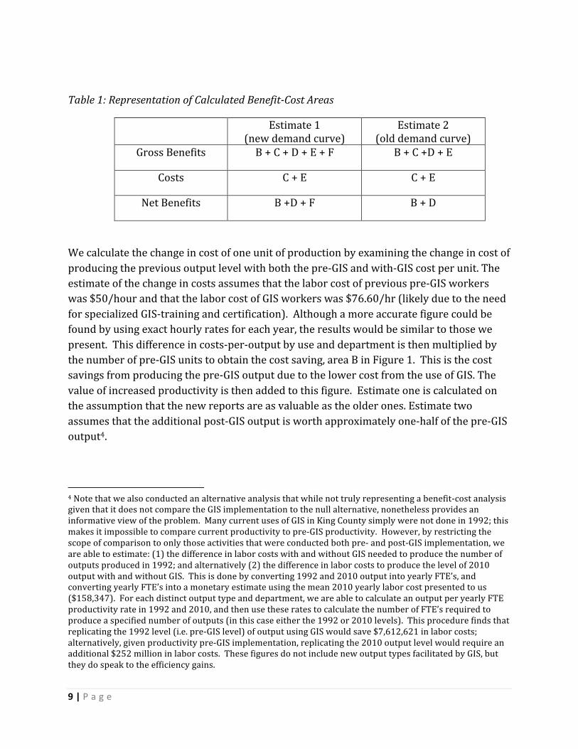
Table 1: Representation of Calculated Benefit-‐Cost Areas

Estimate 1 (new demand curve)

Estimate 2 (old demand curve)

Gross Benefits B + C + D + E + F B + C +D + E

Costs C + E C + E

Net Benefits B +D + F B + D

We calculate the change in cost of one unit of production by examining the change in cost of producing the previous output level with both the pre-‐GIS and with-‐GIS cost per unit. The estimate of the change in costs assumes that the labor cost of previous pre-‐GIS workers was $50/hour and that the labor cost of GIS workers was $76.60/hr (likely due to the need for specialized GIS-‐training and certification). Although a more accurate figure could be found by using exact hourly rates for each year, the results would be similar to those we present. This difference in costs-‐per-‐output by use and department is then multiplied by the number of pre-‐GIS units to obtain the cost saving, area B in Figure 1. This is the cost savings from producing the pre-‐GIS output due to the lower cost from the use of GIS. The value of increased productivity is then added to this figure. Estimate one is calculated on the assumption that the new reports are as valuable as the older ones. Estimate two assumes that the additional post-‐GIS output is worth approximately one-‐half of the pre-‐GIS output4.

4 Note that we also conducted an alternative analysis that while not truly representing a benefit-‐cost analysis given that it does not compare the GIS implementation to the null alternative, nonetheless provides an informative view of the problem. Many current uses of GIS in King County simply were not done in 1992; this makes it impossible to compare current productivity to pre-‐GIS productivity. However, by restricting the scope of comparison to only those activities that were conducted both pre-‐ and post-‐GIS implementation, we are able to estimate: (1) the difference in labor costs with and without GIS needed to produce the number of outputs produced in 1992; and alternatively (2) the difference in labor costs to produce the level of 2010 output with and without GIS. This is done by converting 1992 and 2010 output into yearly FTE’s, and converting yearly FTE’s into a monetary estimate using the mean 2010 yearly labor cost presented to us ($158,347). For each distinct output type and department, we are able to calculate an output per yearly FTE productivity rate in 1992 and 2010, and then use these rates to calculate the number of FTE’s required to produce a specified number of outputs (in this case either the 1992 or 2010 levels). This procedure finds that replicating the 1992 level (i.e. pre-‐GIS level) of output using GIS would save $7,612,621 in labor costs; alternatively, given productivity pre-‐GIS implementation, replicating the 2010 output level would require an additional $252 million in labor costs. These figures do not include new output types facilitated by GIS, but they do speak to the efficiency gains.

10 | P a g e

Results

Table 2 shows the Net Benefits for the year 2010 for the use of GIS. The first estimate assumes no diminution in value; the second assumes the value of additional outputs falls linearly from 1993.

Table 2: Summary of Net Benefit for Year 20105

Assumes Equal Output Value to Pre-‐Gis Production

Assumes Lower Value then Pre-‐Gis Production

Gross Benefits Estimate

$195,640,898 $102,250,606

Costs $14,641,647 $14,641,647 Net Benefits $180,999,251 $87,608,959

These are net benefits for just one recent year.6 Table 3 shows the benefit-‐cost ratio and the project rate of return, two financial summary metrics of project efficiency. The benefit-‐cost ratio is simply the ratio of project benefits over project costs (thus, projects with positive net benefits have a B/C ratio greater than one). Note that the benefit-‐cost ratio is useful for determining whether a project is efficient (as is the goal of this analysis), but cannot be used to compare the benefit of different GIS programs, for instance, when all are found to have positive net benefits. This is because the B/C ratio is scale invariant, such that a project that costs $1 but produces $10 in benefits will have a higher B/C ratio than a project that costs $1 million but produces $10 million in benefits, even though the latter project produces $9 million of net benefit while the former produces only $9.

Table 3: Benefit-‐Cost Ratios for Figures in Table 2.

Estimation Technique B/C Ratio

5 The Cost Calculations for the year 2006 to 2011 are generated from the KCGIS Operations and Management (O&M) Plan. To calculate the effective labor costs, the total labor costs is multiplied with the average percentage of time the staff spend on GIS –related work. Hardware, Software, Training, and other direct non-‐labor costs are then added to the effective Labor Cost to get the Total Cost spent on GIS per year. 6 This Table shows the net benefits under the assumption that all costs apply to 2010 and that benefits are just for 2010.

11 | P a g e

Output of Equal Value 13.36 Output of Lower Value 6.98

The above results strongly suggest that GIS technology is clearly a sound investment for King County. As an exploratory exercise, however, we also extrapolate these results, in conjunction with yearly cost figures provided by the County, to estimate total net benefits accrued over the entire 18-‐year period in which the County has been utilizing GIS technology.

It would not be reasonable to assume that the 2010 benefit figure directly applies for all other years, since: (1) GIS funding has increased significantly over time (from $210,000 in 1992 to about $14 million in 2010), and given the return on investment the 2010 figures speak to, we would expect this increased level of funding to increase the level of benefits; (2) GIS technological capabilities have increased over the time period; and (3) the benefits associated with GIS have likely increased due to network externalities and synergistic effects, as more organizations utilize GIS and more data become available. Thus, we employ two methods of estimating benefits in years prior to 2010, first by linking benefits to the 2010 B/C ratio, and second by linearly extrapolating benefits between 2010 and 1992, assuming $0 benefits in 1992.

Table 4 shows yearly benefit figures estimated using actual cost data and the estimated 2010 B/C ratio. The first two columns of benefits correspond to the prior estimated B/C ratios for 2010 outputs of declining marginal value and constant marginal value. The third column of benefits addresses the issues of network externalities and synergistic effects raised above by reducing the B/C ratio by 10% each year. This 10% figure is obviously an arbitrary parameter, but it at least allows us to examine what the benefit estimates are if we assume that the return to investment in GIS technology has increased as GIS has become more prominently used and the underlying technology has improved.

Table 4: Yearly Benefit Estimates Using B/C Ratio Extrapolation

Year Costs

Benefits (Outputs of Declining Value)

Benefits (Outputs of Constant Value

Benefits (B/C Ratio Increases 10%/yr, declining marginal output value)

1992 $210,000 $1,466,544.53 $2,806,008.68 $263,770.92

1993 $839,667 $5,863,852.58 $11,219,585.20 $1,160,131.97

1994 $2,989,667 $20,878,475.11 $39,947,769.31 $4,543,764.50 1995 $4,672,667 $32,631,781.96 $62,435,924.60 $7,811,789.16

1996 $4,485,000 $31,321,200.95 $59,928,328.26 $8,247,851.13

12 | P a g e

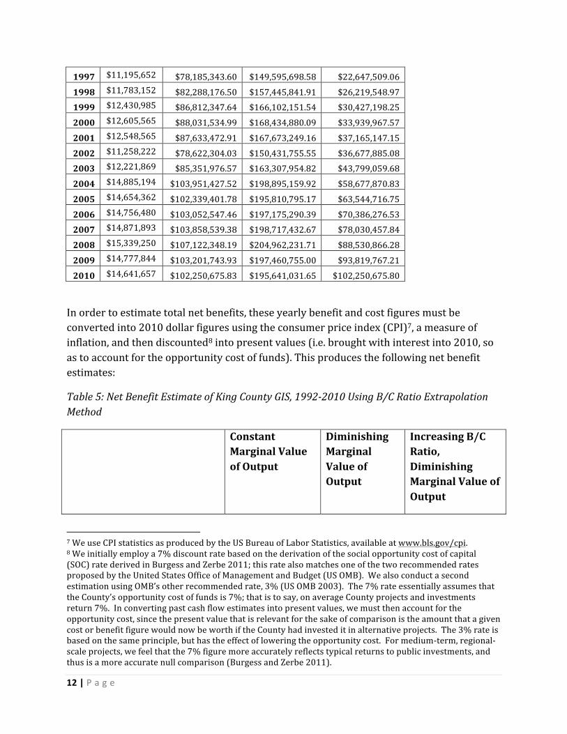
1997 $11,195,652 $78,185,343.60 $149,595,698.58 $22,647,509.06

1998 $11,783,152 $82,288,176.50 $157,445,841.91 $26,219,548.97 1999 $12,430,985 $86,812,347.64 $166,102,151.54 $30,427,198.25

2000 $12,605,565 $88,031,534.99 $168,434,880.09 $33,939,967.57

2001 $12,548,565 $87,633,472.91 $167,673,249.16 $37,165,147.15

2002 $11,258,222 $78,622,304.03 $150,431,755.55 $36,677,885.08 2003 $12,221,869 $85,351,976.57 $163,307,954.82 $43,799,059.68

2004 $14,885,194 $103,951,427.52 $198,895,159.92 $58,677,870.83

2005 $14,654,362 $102,339,401.78 $195,810,795.17 $63,544,716.75

2006 $14,756,480 $103,052,547.46 $197,175,290.39 $70,386,276.53 2007 $14,871,893 $103,858,539.38 $198,717,432.67 $78,030,457.84

2008 $15,339,250 $107,122,348.19 $204,962,231.71 $88,530,866.28

2009 $14,777,844 $103,201,743.93 $197,460,755.00 $93,819,767.21

2010 $14,641,657 $102,250,675.83 $195,641,031.65 $102,250,675.80

In order to estimate total net benefits, these yearly benefit and cost figures must be converted into 2010 dollar figures using the consumer price index (CPI)7, a measure of inflation, and then discounted8 into present values (i.e. brought with interest into 2010, so as to account for the opportunity cost of funds). This produces the following net benefit estimates:

Table 5: Net Benefit Estimate of King County GIS, 1992-‐2010 Using B/C Ratio Extrapolation Method

Constant Marginal Value of Output

Diminishing Marginal Value of Output

Increasing B/C Ratio, Diminishing Marginal Value of Output

7 We use CPI statistics as produced by the US Bureau of Labor Statistics, available at www.bls.gov/cpi. 8 We initially employ a 7% discount rate based on the derivation of the social opportunity cost of capital (SOC) rate derived in Burgess and Zerbe 2011; this rate also matches one of the two recommended rates proposed by the United States Office of Management and Budget (US OMB). We also conduct a second estimation using OMB’s other recommended rate, 3% (US OMB 2003). The 7% rate essentially assumes that the County’s opportunity cost of funds is 7%; that is to say, on average County projects and investments return 7%. In converting past cash flow estimates into present values, we must then account for the opportunity cost, since the present value that is relevant for the sake of comparison is the amount that a given cost or benefit figure would now be worth if the County had invested it in alternative projects. The 3% rate is based on the same principle, but has the effect of lowering the opportunity cost. For medium-‐term, regional-‐scale projects, we feel that the 7% figure more accurately reflects typical returns to public investments, and thus is a more accurate null comparison (Burgess and Zerbe 2011).

13 | P a g e

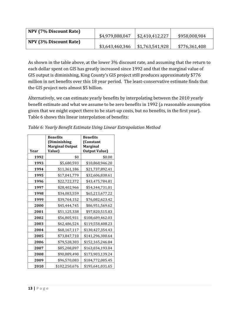
NPV (7% Discount Rate) $4,979,888,047 $2,410,412,227 $958,008,984

NPV (3% Discount Rate) $3,643,460,346 $1,763,541,928 $776,361,408

As shown in the table above, at the lower 3% discount rate, and assuming that the return to each dollar spent on GIS has greatly increased since 1992 and that the marginal value of GIS output is diminishing, King County’s GIS project still produces approximately $776 million in net benefits over this 18 year period. The least-‐conservative estimate finds that the GIS project nets almost $5 billion.

Alternatively, we can estimate yearly benefits by interpolating between the 2010 yearly benefit estimate and what we assume to be zero benefits in 1992 (a reasonable assumption given that we might expect there to be start-‐up costs, but no benefits, in the first year). Table 6 shows this linear interpolation of benefits:

Table 6: Yearly Benefit Estimate Using Linear Extrapolation Method

Year

Benefits (Diminishing Marginal Output Value)

Benefits (Constant Marginal Output Value)

1992 $0 $0.00 1993 $5,680,593 $10,868,946.20 1994 $11,361,186 $21,737,892.41 1995 $17,041,779 $32,606,838.61 1996 $22,722,372 $43,475,784.81 1997 $28,402,966 $54,344,731.01 1998 $34,083,559 $65,213,677.22 1999 $39,764,152 $76,082,623.42 2000 $45,444,745 $86,951,569.62 2001 $51,125,338 $97,820,515.83 2002 $56,805,931 $108,689,462.03 2003 $62,486,524 $119,558,408.23 2004 $68,167,117 $130,427,354.43 2005 $73,847,710 $141,296,300.64 2006 $79,528,303 $152,165,246.84 2007 $85,208,897 $163,034,193.04 2008 $90,889,490 $173,903,139.24 2009 $96,570,083 $184,772,085.45 2010 $102,250,676 $195,641,031.65

14 | P a g e

Using these estimates, first subtracting yearly costs and then converting into 2010 dollars (using the CPI), and finally bringing “forward” into present value (using the discount rate), we get the following net benefit estimates:

Table 7: Net Benefit Estimate of King County GIS, 1992-‐2010 Using Linear Interpolation Method

Constant Marginal Value of Output

Diminishing Marginal Value of Output

NPV (7% Discount Rate) $2,975,060,281 $1,362,600,363

NPV (3% Discount Rate) $2,275,897,398 $1,048,792,908

ROI (7% Discount Rate) 13.8% 9.7%

ROI (3% Discount Rate) 13.8% 9.9%

Thus, the linear interpolation method also estimates that King County’s GIS project has produced significant net benefits, at least $1 billion even in the most conservative estimate (since each yearly cash flow is positive, the lower discount rate serves to reduce the overall benefit level). Similarly, the Return on Investment (ROI) figure demonstrates that the GIS project is beneficial as well, since the return rate is greater than the discount rate (either 3% or 7%) in both cases.9 Thus, we again estimate that King County’s GIS program returns greater net benefits than might be received were the same funds applied to an average project or investment. As discussed previously, Burgess and Zerbe (2011) find that from a societal perspective, the Social Opportunity Cost of Funds (SOC) is about 7%. Thus the GIS investment appears beneficial not only to King County from an organizational perspective, but also to society at large.

9 The rate of return on investment is calculated as ROI = [(Future Value Benefits)/Present Value Costs](1/years)-‐1. This formula is derived in Zerbe and Dively (1994). It is similar to the Internal Rate of Return but without the same defects. Essentially, what the ROI figure demonstrates is the interest rate an alternative investment would have to receive in order to provide net benefits equal to the project in question. Thus, if the appropriate discount rate is less than the ROI, a project is a good investment, since it yields a greater return than alternative policy investments.

15 | P a g e

Conclusion

Using any of our estimation methods, our survey and resultant analysis indicates that King County’s GIS program is an excellent policy investment. Even by our most conservative estimate (in which we discount past cash flows at 3%, assume a diminished value for outputs in excess of 1992 levels, and interpolate past benefits using a B/C ratio that decreases by 10% per year), King County’s GIS program is estimated to have earned $776,361,408 in net benefits from 1992 to 2010. It is important to note, however, that this figure is estimated in comparison to the output of county agencies without GIS technology. For any future policy decision-‐making, an analysis would need to consider not only the null comparison of not funding any GIS technology, but also various levels of GIS funding and different types of GIS technology, since this is the true rubric against which any future GIS policy should be compared.

The estimated net benefit figures are extremely high, likely much higher than the “true” level of benefits. One difficulty in the survey method was the inability to disentangle efficiency gains facilitated from technological advance more broadly and GIS-‐specific benefits. For instance, advancement in computational ability, productivity software, and connectivity are inextricably linked to the use (and benefits) of GIS. Thus, our estimates of the net benefits of GIS technology are expected to be at least partially conflated with efficiency gains facilitated by these other technological advances. In essence, the efficiency gains are likely overestimated, since our survey was unable to avoid an implicit comparison between not only agency output with and without GIS, but also agency output in 1992 and 2010. However, this should not detract from the fact that King County’s investment in GIS technology has been sound. The net benefits estimates are so resoundingly high that we are certain that GIS technology has engendered positive net benefits for the County in any case.

Moreover, our analysis accounts for all costs (since these are tabulated directly), but only a subset of benefits. The survey technique compared only efficiency gains related to the production of outputs; that is, we account for the fact that GIS enables the County to produce the same geospatial outputs it produced without GIS but with less effort (FTE savings) and the fact that GIS enables the County to produce new, beneficial geospatial outputs that are enabled by the presence of GIS (gains in increased production). For instance, a significant benefit of GIS technology is the usefulness of GIS data and geospatial presentation capabilities. Using the production with-‐and-‐without survey methodology, we are unable to capture benefits such as the ability to access geospatial data via a mobile device, benefits associated with new types of outputs (since there is no prior comparison),

16 | P a g e

and increased modeling, analytical, and research capabilities made possible by GIS technology. Thus, the overestimation of benefits associated with the estimated efficiency and output gains is likely tempered in part by the exclusion of these additional benefit categories.

Lastly, the results of this analysis have significant implications for conducting similar analyses in the future. Given resource constraints and public demands for accountability, it is important for government agencies to be able to monitor the performance of policy projects. Such analyses can guide future policy decision-‐making, evidence the effectiveness of current efficient policies, and identify inefficient government investments that detract from social welfare. In refining the with-‐and-‐without survey design suing the ROI model, we identify several key points:

This technique is better applicable to some types of policies and projects than others.

a. Projects well suited to this methodology involve: i. Well-‐defined job descriptions ii. Discrete, well-‐delineated employee tasks iii. Discrete, aggregatable outputs iv. Good data regarding project costs v. A discrete divide between before and after states

b. Projects poorly suited for this methodology involve: i. Continuous, poorly-‐delineated tasks ii. Poorly aggregatable outputs iii. Qualitative output improvements

Applying this rubric to the analysis of King County’s GIS initiative, we can readily see areas in which this project was well-‐suited for this methodology, and others in which aspects of the project made analysis very difficult. Since the GIS project was funded via a top down model through King County’s GIS Center, cost data was easily attainable. In this case, we can be completely confident in the figures on the cost side of the ledger, whereas cost data would have been much more difficult to tease out had resources been allocated at lower levels within County agencies or had GIS costs not been separately delineated within the budget.

One of the primary GIS outputs incorporated into this analysis, maps, is well-‐suited in some respects for this technique, and poorly suited in others. This might not at first appear to be the case, since while maps are often a discrete output, GIS technology also allows maps to build on one another and continuously be updated and revised. However, while there is a significant difference between a completely new map that must be generated first by geocoding new points of interest or analyzing geospatial data and a map that is quickly produced by layering on features already coded into the database, the with-‐and-‐without

17 | P a g e

design largely accounts for this discrepancy by also asking about the change in FTEs required to produce said outputs. Thus, we can control for heterogeneous output characteristics using the effort required to produce said output. However, this method is highly dependent on the way in which the survey respondent defines the unit of output. A “map” might mean very different things to different employees, thus hindering our ability to aggregate an increase in map production across these individuals.

Given that GIS technology is utilized by trained professionals, often with special certification in the use of GIS, job descriptions and employee tasks are largely discrete and well-‐defined. If GIS technology was utilized as a small component of every agency employee’s job, rather than being utilized as a significant component by a specialized subset of employees, estimation would have been much more difficult, since the diversity of tasks and outputs within an agency would have made estimation by survey respondents much more difficult and also greatly hindered output aggregation.

The clearly delineated implementation point of GIS is key to the success of this analysis, since respondents must be able to clearly delineate between their production before and after project implementation. Note that there are certain tradeoffs associated with the “bandwidth” used for the before-‐and-‐after comparison. Immediately following GIS implementation (in this case in 1993), respondents would have been able to very accurately assess their change in production level and job behavior. Moreover, as discussed previously, as the comparison periods grow further apart, estimates can become conflated with other technological advancements. However, there is most certainly a learning period and ramp-‐up effect to GIS as employees become more familiar with its use and better integrate the technology into daily operations. Thus, asking respondents to compare their pre-‐GIS output in 1992 with their current GIS-‐facilitated output more accurately captures the true benefits associated with GIS, that were likely not as apparent shortly after implementation.

Lastly, one aspect of GIS technology that is poorly suited for this methodology is the qualitative improvement of GIS-‐produced outputs relative to pre-‐GIS outputs. We assume that the GIS outputs are simply more useful and allow the County to utilize geospatial data in new and more efficient ways. The with-‐and-‐without design cannot account for this, since it assesses the quantitative change in outputs under the assumption that outputs created before and after implementation are otherwise homogenous.

18 | P a g e

References

Textual References Burgess, David F., and Richard O Zerbe. 2011. "Calculating the Social Opportunity Cost

Discount Rate". Journal of Benefit-‐Cost Analysis. 2(3). US OMB (Office of Management and Budget). 2003. Informing Regulatory Decisions: 2003

Report to Congress on the Costs and Benefits of Federal Regulations and Unfunded Mandates on State, Local, and Tribal Entities. Washington, D.C.: US Government Printing Office.

Zerbe, Richard O., and Dwight Dively. 1994. Benefit-‐cost analysis in theory and practice. New York: HarperCollins College Publishers.

Zerbe, R.O., T.B. Davis, N.S. Garland, and T.S. Scott. 2010. Towards Principles and Standards

in the Use of Benefit-‐Cost Analysis: A Summary of Work, and a Starting Place. MacArthur Foundation Power of Measuring Social Benefits Initiative. Seattle, WA: Benefit-‐Cost Analysis Center, University of Washington.

PlanGraphics Inc., Studies for 1992 King County GIS Plan:

Croswell, P., Metcalf, A. Smith, C. & Hiday, A. King County GIS Needs Assessment/Applications Working Paper. Frankfort, KY: Plangraphics, Inc. 1992.

Croswell, P., Metcalf, A. Smith, C. Anderson, J. & Schlosser, J. King County GIS Conceptual Design. Frankfort, KY: Plangraphics, Inc. 1992.

Croswell, P., Metcalf, A. & Ahner, A. King County GIS Benefit/Cost Report, Frankfort, KY: Plangraphics, Inc. 1992.

Croswell, P., Metcalf, A. & Schlosser, J. King County GIS Implementation and Funding Plan, Frankfort, KY: Plangraphics, Inc. 1992.

King County internal documentation:

Babinski, Greg. King County GIS Technical Committee Issue #4 Report: Status of Original GIS Capital Project Work Tasks, August 26, 2003

King County Coordinated GIS Scoping Project. August 1993.

19 | P a g e

King County GIS Technical Committee: King County GIS Annual O&M Plans 1997, 2002-‐2010.

Metro 1993 GIS Alternatives Analysis and Recommendation, 1993

GIS References

Croswell, Peter L. The GIS Management Handbook. Frankfort, KY: Kessey Dewitt Publications, 2009.

Lerner, Nancy, Ancel, Susan, Stewart, Mary Ann, and DiSera. Dave. Building a Business Case for Geospatial Technology: A Practitioner’s Guide to Financial and Strategic Analysis. Geospatial Information Technology Association and AWWA Research Foundation, 2007.

Maguire, David, Kouyoumjian, and Smith, Ross. The Business Benefits of GIS: An ROI Approach. Redlands: ESRI Press, 2008.

Thomas, Christopher and Ospina, Milton. Measuring Up: The Business Case for GIS. Redlands: ESRI Press, 2004.

20 | P a g e

Appendices

A. PERTINENT SURVEY QUESTIONS

Please estimate the number of each output you currently produce (in 2010), being clear about the time frame (per day, per year, etc.). Also state the total number of outputs from your agency (if known), and the number of employees and full-‐time employees (FTEs) currently working on producing this output. If you answered that you did not produce a given output in the previous section, you may skip the personal production questions.

• How many units of this output do you personally produce? Choose # of units: • How many units of this output do you personally produce Per Unit of Time: • What percent of your time do you spend producing each output now? (%) • What percent of your time do you spend producing each output now: Per Unit

of Time: • Number of Employees in your workgroup (including you) currently producing

this output: • Total FTEs in your workgroup (including you) currently producing this output:

Again, the outputs commonly produced by your agency are listed below in the first column. If you were not present when the output was produced without GIS, please answer No to the first question but provide your best estimate for the remaining questions. For each output, please indicate how having GIS has impacted labor productivity for you personally and for your agency overall.

• Did you personally produce this output without GIS? • How many units of this output did you personally produce prior to GIS? Choose # of

units: • How many units of this output did you personally produce Per Unit of Time prior to

GIS: • What percent of your time did you spend producing each output prior to GIS? (%) • What percent of your time did you spend producing each output Prior to GIS: Per

Unit of Time: • Number of Employees in your workgroup (including you) producing this output

prior to GIS:

Total FTEs in your workgroup (including you) producing this output prior to GIS:

21 | P a g e

B. Cost Calculations per Year

Table 8: Yearly GIS Costs as Provided by King County GIS Center

Year Cost

1992 $210,000

1993 $839,667

1994 $2,989,667

1995 $4,672,667

1996 $4,485,000

1997 $11,195,652

1998 $11,783,152

1999 $12,430,985

2000 $12,605,565

2001 $12,548,565

2002 $11,258,222

2003 $12,221,869

2004 $14,885,194

2005 $14,654,362

2006 $14,756,480

2007 $14,871,893

2008 $15,339,250

2009 $14,777,844

2010 $14,641,657

Total: $201,167,690

22 | P a g e

C. Benefit Calculations at Different Rates

Adjustment for lower salaries for pre-‐GIS Table 6 below shows net benefits under alternative assumptions. We assume alternatively the lower pre-‐GIS labor costs for workers – $50/hour and the alternate of $76.60/hour used in the initial analysis – to compute the aggregate benefits. This results in lower estimates in the total aggregate benefits as compared with the original analysis.

Table 9: Summary Net Benefits for 2010

Benefits at Different Wage Rates in the Pre-‐GIS era

Gross Benefits per year from cost savings

Benefits per year from increased productivity

Total Gross Benefits per year assuming diminution in quality of output

Total Benefits Assuming no diminution in quality of GIS products

Aggregate Benefits at $76.60/hour for post GIS $11,125,727 $148,832,675 $159,958,402

$308,791,077

Aggregate Benefits at $50/hour for pre-‐GIS $3,985,667

$93,390,293 $97,375,961

$190,766,253

23 | P a g e

D. Benefits by department at different labor rates

Benefits by Use for 2010

Table 10: Benefits from the Use of GIS: Aggregate Benefits at $76.60/hour for Post-‐GIS Output

Output

Benefits from cost savings of producing pre-‐GIS output with GIS technology =

Benefits from Productivity Increases Assuming Quality Remains the Same as Pre-‐GIS Quality

Benefits from increased productivity Assuming Quality Falls

Total Benefits with Quality Constant

Total benefits Assuming Quality Falls = Benefits from cost savings + Benefits from increased outputs

Qpre-‐GIS * Δ$/unit

= (1/2)*ΔQ* Δ$/unit

DATA

COLLECTION AND DATA MANAGEMENT

-‐5,701,747 51,763,374 25,881,687 46,061,627 20,179,940

MAPPING 7,664,566 34,295,466 17,147,733 41,960,032 24,812,299 SPATIAL

ANALYSIS 2,936,612 51,599,782 25,799,891 54,536,394 28,736,503

MAPS OR SPATIAL ANALYSIS IN SUPPORT OF PUBLIC RELATIONS, COMMUNICATIONS OR WEBSITE

2,434,981 23,110,264 11,555,132 25,545,245 13,990,113

ACTVITIES & ASSET MONITORING

1,263,477 * 6,,949,124 * 8,212,601

PLANNING * 1,063,300 531,650 * 531,650 CUSTOM DATA,

MAPPING & APPLICATION

-‐175,941 28,691,370 14,345,685 28,515,429 14,169,744

24 | P a g e

REQUESTS ENVIRONMENTAL MONITORING 1,288,553 84,998,970 42,499,485 86,287,523 43,788,038

PERMITTING 1,256,879 3,770,638 1,885,319 5,027,517 3,142,198 LEVY &

ANNEXATION 0 158,346 79,173 158,346 79,173

APPRAISALS 0 316,694 158,347 316,694 158,347 OTHER 158,347 3,998,896 1,999,448 4,157,243 2,157,795 TOTAL NET

BENEFITS PER YEAR

$11,125,727

297,665,350

$148,832,675

308,791,077

$159,958,402

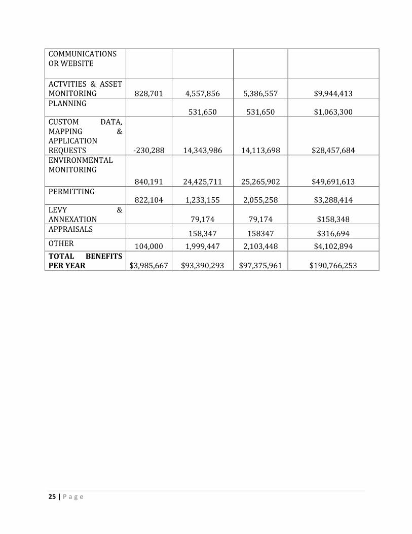
Table 11: Benefits from use of GIS – Aggregate Results by Output at $50 per hour cost for Pre-‐GIS Output

Output Benefits from cost savings =

Qpre-‐GIS * Δ$/unit

Benefits from increased productivity

= (1/2)*ΔQ* Δ$/unit

Total benefits assuming Quality falls = Benefits from cost savings + Benefits from increased outputs

Best Estimate Benefits Assuming Quality Remains Same = Benefits from Cost Saving + Benefits from increased output (*ΔQ* Δ$/unit)

DATA COLLECTION AND DATA MANAGEMENT -‐6,197,664 13,452,087 7,254,423 $20,706,510 MAPPING

4,822,975 10,568,953 15,391,928 $25,968,081 SPATIAL ANALYSIS

1,672,989 15,395,389 17,068,378 $35,613,753 MAPS OR SPATIAL ANALYSIS IN SUPPORT OF PUBLIC RELATIONS, 1,322,660 6,644,538 7,967,198 $7,967,198

25 | P a g e

COMMUNICATIONS OR WEBSITE

ACTVITIES & ASSET MONITORING 828,701 4,557,856 5,386,557 $9,944,413 PLANNING

531,650 531,650 $1,063,300 CUSTOM DATA, MAPPING & APPLICATION REQUESTS -‐230,288 14,343,986 14,113,698 $28,457,684 ENVIRONMENTAL MONITORING

840,191 24,425,711 25,265,902 $49,691,613 PERMITTING

822,104 1,233,155 2,055,258 $3,288,414 LEVY & ANNEXATION 79,174 79,174 $158,348 APPRAISALS 158,347 158347 $316,694 OTHER 104,000 1,999,447 2,103,448 $4,102,894 TOTAL BENEFITS PER YEAR $3,985,667 $93,390,293 $97,375,961 $190,766,253

26 | P a g e

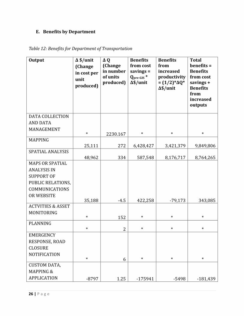
E. Benefits by Department

Table 12: Benefits for Department of Transportation Output ∆ $/unit

(Change in cost per unit produced)

∆ Q (Change in number of units produced)

Benefits from cost savings = Qpre-‐GIS * Δ$/unit

Benefits from increased productivity = (1/2)*ΔQ* Δ$/unit

Total benefits = Benefits from cost savings + Benefits from increased outputs

DATA COLLECTION AND DATA MANAGEMENT

* 2230.167 * * * MAPPING

25,111 272 6,428,427 3,421,379 9,849,806 SPATIAL ANALYSIS

48,962 334 587,548 8,176,717 8,764,265 MAPS OR SPATIAL ANALYSIS IN SUPPORT OF PUBLIC RELATIONS, COMMUNICATIONS OR WEBSITE

35,188 -‐4.5 422,258 -‐79,173 343,085 ACTVITIES & ASSET MONITORING

* 152 * * * PLANNING

* 2 * * * EMERGENCY RESPONSE, ROAD CLOSURE NOTIFICATION

* 6 * * * CUSTOM DATA, MAPPING & APPLICATION -‐8797 1.25 -‐175941 -‐5498 -‐181,439

27 | P a g e

REQUESTS

OTHER * 0 * * *

TOTAL BENEFITS FOR DOT/ YEAR

$7,262,292

$11,513,425

$18,775,718

Table 12: Benefits for Department of Natural Resources and Parks (Except Wastewater)

Output ∆ $/unit (Change in cost per unit produced)






26,521 1,853 13,260 24,577,214 24,590,475 MAPPING

* 664 * * * SPATIAL ANALYSIS

22932 463 11,466 5,312,686 5,324,152 MAPS OR SPATIAL ANALYSIS IN SUPPORT OF PUBLIC RELATIONS, COMMUNICATIONS OR WEBSITE

* 201 * * * ACTVITIES & ASSET MONITORING

* * * * * ENVIRONMENTAL MONITORING

31,674 2,564 31,674 40,614,166 40,645,840 PLANNING

* 34 * 531,650 531,650

28 | P a g e

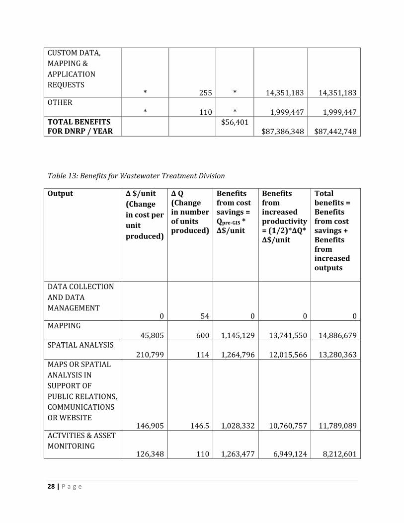
CUSTOM DATA, MAPPING & APPLICATION REQUESTS

* 255 * 14,351,183 14,351,183 OTHER

* 110 * 1,999,447 1,999,447 TOTAL BENEFITS FOR DNRP / YEAR

$56,401 $87,386,348 $87,442,748

Table 13: Benefits for Wastewater Treatment Division







0 54 0 0 0 MAPPING

45,805 600 1,145,129 13,741,550 14,886,679 SPATIAL ANALYSIS

210,799 114 1,264,796 12,015,566 13,280,363 MAPS OR SPATIAL ANALYSIS IN SUPPORT OF PUBLIC RELATIONS, COMMUNICATIONS OR WEBSITE

146,905 146.5 1,028,332 10,760,757 11,789,089 ACTVITIES & ASSET MONITORING

126,348 110 1,263,477 6,949,124 8,212,601

29 | P a g e

PLANNING * -‐3 * * *

ENVIRONMENTAL MONITORING

83,792 45 1,256,879 1,885,319 3,142,198 PERMITTING

139,653 27 1,256,879 1,885,319 3,142,198 OTHER

-‐164.945 * * * * TOTAL BENEFITS FROM WASTEWATER PER YEAR

$7,215,493

$47,237,636

$54,453,130

Table 14: Benefits for Department of Assessment







-‐414 -‐6,680 -‐6,031,702 1,383,646 -‐4,648,056 MAPPING

-‐48 3070 -‐265,271 -‐74,577 -‐339,848 SPATIAL ANALYSIS

7,917 80 158,347 316,694 475,041 MAPS OR SPATIAL ANALYSIS IN SUPPORT OF PUBLIC RELATIONS, COMMUNICATIONS OR WEBSITE

138 9,100 752,148 626,790 1,378,939 LEVY &

7,917 20 0 79,173 79,173

30 | P a g e

ANNEXATIONS

APPRAISALS 15,835 20 0 158,347 158,347

OTHER

3,045 0 158,347 0 158,347

TOTAL BENEFIT FROM ASSESSMENT PER YEAR

$-‐5,228,130

$2,490,074

$ -‐2,738,057

Table 15: Other Departments







7,917 -‐20 316,694 -‐79,173 237,520 MAPPING

4,750 25 356,280 59,380 415,660 SPATIAL ANALYSIS

17,418 -‐2.5 914,453 -‐21,772 892,681 MAPS OR SPATIAL ANALYSIS IN SUPPORT OF PUBLIC RELATIONS, COMMUNICATIONS OR WEBSITE

7257.571 68 232,242 246,757 478,999 TOTAL BENEFIT FROM OTHER PER YEAR

$1,819,670 $205,191 $2,024,862

31 | P a g e

F. Discussion of Anomalies In Department/Usage Calculations

Departments and Uses

There are two negative results for particular GIS uses within the Department of Assessment and one within the Department of Transportation. For the Department of Assessment these are for Data Collection and Data Management and also for the Custom Data, Mapping, and Application requests. While the former result is driven by both a significant decrease in total output produced as well as an increase in cost per unit production from the pre to the post GIS period in the Department of Assessment, the latter result is specifically driven by an increase in cost per unit of production from the pre to post period.

We can only speculate about the reasons for these results. A closer look at the number of Full Time Employees (FTE’s) working at the Department of Assessment shows that the number has decreased during the post-‐GIS period. This could put additional burden on the existing labor force thereby increasing their cost of labor per unit of production. Furthermore, the capabilities of GIS could possibly stretch the labor force in new directions by making Data Collection and Data Management a more resource intensive procedure than it was before – therefore, although the quantity of output might not change, the quality could have in terms of producing outputs with a higher information content, which is not captured in our analysis.

32 | P a g e

G. PERCENTAGE CHANGE IN PRODUCTIVITY & INPUTS

Table 16 Percentage Change in Productivity Associated with GIS – Aggregate Results

Output % Change in OUTPUT with fixed Labor

% Change in OUTPUT with fixed Time

% Change in OUTPUT with fixed Computer Equipment and Supplies

% Change in OUTPUT with fixed Office/Print Equipment & Supplies


68.65% 52.26% 44% 36.66%

MAPPING 81.65% 70.26% 49.31% 36.25%

SPATIAL ANALYSIS 107.5% 83.3% 43.16% 50%

MAPS OR SPATIAL ANALYSIS IN SUPPORT OF PUBLIC RELATIONS, COMMUNICATIONS OR WEBSITE 62.66% 70.75% 50% 75%


50% 55% * 10%

PLANNING 40% 21.66% 30% 15%

CUSTOM DATA, MAPPING & APPLICATION REQUESTS

62.50% 50% 30% 40%


47.5% 27.5% 5% *

OTHER 5% 27.5% 10% *

33 | P a g e

Table 17: Percentage Change in Input Associated with GIS – Aggregate Results

Output % Change in LABOR with fixed output

% Change in TIME with fixed output

% Change in COMPUTER EQUIPMENT and SUPPLIES with fixed output

% Change in OFFICE/PRINT EQUIPMENT & SUPPLIES with fixed output

DATA COLLECTION AND DATA MANAGEMENT -‐40% -‐39.5% 71% 19.75%

MAPPING -‐37.35% -‐45.85% 39.6% 27%

SPATIAL ANALYSIS -‐55% -‐62.5% 72.5% 40%

MAPS OR SPATIAL ANALYSIS IN SUPPORT OF PUBLIC RELATIONS, COMMUNICATIONS OR WEBSITE

-‐38.2% -‐43.5% 56.6% 48.25%


-‐17.5% -‐17.5% -‐5% -‐10%

PLANNING -‐17.5% -‐10.8% 3.5% -‐20%

CUSTOM DATA, MAPPING & APPLICATION REQUESTS -‐36.25% -‐40% 27.5% 8.75%


-‐20% -‐20% * -‐20%

OTHER -‐30% -‐35% 10% -‐10%

34 | P a g e

H. King County GIS Center/State of Oregon Project Team

King County GIS Center Project Manager:

-‐Greg Babinski

State of Oregon Project Lead

-‐Cy Smith, GISP, State of Oregon GIO

King County GIS Center Interview Team: -‐-‐-‐George Horning, KCGIS Center Manager -‐-‐-‐Greg Stought, Enterprise Services Manager -‐-‐-‐Dennis Higgins, GISP, Client Services Manager -‐-‐-‐Debbie Bull, GIS DBA -‐-‐-‐Greg Babinski, GISP, Finance & Marketing Manager

an analysis of benefits from use of geographic information ... · an analysis of benefits from use...

Documents