An Energy Management Controller to Optimally Trade Off FuelEconomy and Drivability for Hybrid Vehicles

Daniel F. Opila, Xiaoyong Wang, Ryan McGee, R. Brent Gillespie, Jeffrey A. Cook, and J.W. Grizzle

Abstract—Hybrid Vehicle fuel economy performance is highlysensitive to the energy management strategy used to regulatepower flow among the various energy sources and sinks. Optimalnon-causal solutions are easy to determine if the drive cycleis known a priori. It is very challenging to design causalcontrollers that yield good fuel economy for a range of possibledriver behavior. Additional challenges come in the form ofconstraints on powertrain activity, such as shifting and startingthe engine, which are commonly called “drivability” metricsand can adversely affect fuel economy. In this paper, drivabilityrestrictions are included in a Shortest Path Stochastic DynamicProgramming (SP-SDP) formulation of the real-time energymanagement problem for a prototype vehicle, where the drivecycle is modeled as a stationary, finite-state Markov chain. Whenthe SP-SDP controllers are evaluated with a high-fidelity vehiclesimulator over standard government drive cycles, and comparedto a baseline industrial controller, they are shown to improvefuel economy more than 11% for equivalent levels of drivability.In addition, the explicit tradeoff between fuel economy anddrivability is quantified for the SP-SDP controllers.

I. INTRODUCTION

Hybrid vehicles have become increasingly popular in theautomotive marketplace in the past decade. The most commontype is the electric hybrid, which consists of an internalcombustion engine (ICE), a battery, and at least one electricmachine (EM). Hybrids are built in several configurationsincluding series, parallel, and the series-parallel configurationconsidered here. Hybrid vehicles are characterized by multipleenergy sources; the strategy to control the energy flow amongthese multiple sources is termed “energy management” and iscrucial for good fuel economy. An excellent overview of thisarea is available in [4].

The energy management problem has been studied exten-sively in academic circles. Various control design methods areused, including rule-based [5], [6], [7], [8], neural networks[9], game theory [10], and fuzzy logic [11]. There are manyproposed methods available for both the non-causal (cycleknown in advance) and causal (cycle unknown in advance)cases [12], [13], [14], as well as those with partial futureinformation [15], [16]. The most commonly used optimizationstrategies are the Equivalent Consumption Minimization Strat-egy (ECMS) [17], [18], [19], [20], [21], [22] and Stochastic

This material is based upon work supported under a National ScienceFoundation Graduate Research Fellowship. D.F. Opila is supported by NDSEGand NSF-GRFP fellowships. D.F. Opila, J.A. Cook, and J.W. Grizzle weresupported by a grant from Ford Motor Company. Portions of this work haveappeared in [1], [2], [3].

Daniel Opila and Brent Gillespie are with the Dept. of Mechanical En-gineering, University of Michigan.{dopila,brentg}@umich.eduXiaoyong Wang and Ryan McGee are with Ford Motor Company,Dearborn, MI. Jeffrey Cook and Jessy Grizzle are with the Dept. ofElectrical Engineering and Computer Science, University of Michigan.{jeffcook,grizzle}@umich.edu

or Deterministic Dynamic Programming [23], [24], [25], [26].The majority of existing work focuses on controllers thatseek to minimize fuel consumption, while ignoring otherattributes that affect the smoothness and responsiveness ofvehicle acceleration, which are commonly referred to as“drivability.” In practice, fuel-optimal controllers can lead toexcessive gear shifting and engine starting/stopping [27], [28],[29], [30], and hence poor drivability. Previous research hasaddressed drivability in a suboptimal manner by incorporatingpenalties on engine starts in an ECMS formulation [18]. Thereference [31] addressed engine starts indirectly by includinga hysteresis term “to avoid a too frequent switch on - switchoff of the [internal combustion] engine, which would cause anadditional energy use and wearout.”

In this paper, drivability restrictions are directly incor-porated in a causal, optimal controller design method forthe energy management system of a Hybrid Electric Vehicle(HEV). The focus is on drivability with respect to engine start-stop and gear shifts; a host of other drivability issues, suchas low-frequency longitudinal vibration and other attributeswhich are typically mitigated by hardware design or low-levelcontrol actions, are not considered. The main optimizationtool is Shortest Path Stochastic Dynamic Programming (SP-SDP), which, as explained in [32], [33], [34], [26], is a specificformulation of Stochastic Dynamic Programming (SDP) thatallows infinite horizon optimization problems to be addressedwithout the use of discounting (a discount factor in the costfunction assures convergence by weighting future costs expo-nentially less than current costs). In the energy managementproblem, the power requested by the driver as a function oftime is modeled as a stationary, finite-state Markov chain [23].The state space of the Markov chain is constructed to includea terminal state corresponding to key-off [26]. The terminalstate is designed to be absorbing (that is, it is reached in finitetime with probability one, and there is zero probability oftransitioning out of it). If zero cost is incurred in the absorbingterminal state, then the expected value of the cost function isfinite, even without the discount factor often used in hybridvehicle applications of SDP [33], [34].

The controllers generated through SP-SDP are causal statefeedbacks and hence are directly implementable in a real-timecontrol architecture. The controllers are provably optimal if thedriving behavior matches the assumed Markov chain model.In this paper, the Markov chains representing driver behaviorare modeled on standard government test cycles, as in [23],[26]. It is also possible to build the Markov chains on the basisof real-world driving data, as reported in [35].

In addition to generating a class of optimal controllers,the SP-SDP method allows direct study of the tradeoffsbetween different performance goals, here, drivability and

1

fuel economy. The ability to easily generate Pareto tradeoffcurves is perhaps just as interesting as a specific fuel economybenefit. The designer can generate both the maximum attain-able performance curve and causal controllers that generatethe computed performance. Drivability is emphasized in thispaper, but one could also study the fuel economy tradeoffwith other attributes such as emissions, battery wear, or enginenoise characteristics.

One place where SP-SDP can have a major impact isin controller design for new vehicles. Significant effort isrequired to develop a controller for a new drivetrain, especiallywith a completely new architecture. The SP-SDP method canautomatically generate a provably optimal controller for agiven vehicle architecture and component sizing much fasterthan a person could do it manually.

The work reported here is a collaborative effort between theUniversity of Michigan and Ford Motor Company. The vehiclestudied is a modified Volvo S-80 prototype and does not matchany vehicle currently on the market. As a benchmark, Fordprovided a controller developed for this prototype vehicle.This industrial controller was described in [2] and is termedhereafter the “baseline” controller. In addition, a high-fidelityvehicle simulation model calibrated for the prototype vehiclewas provided; this is the same simulation model used byFord to develop HEV control algorithms and to evaluate fueleconomy and drivability for production vehicles [36].

The remainder of the paper is organized as follows. Sec-tion II presents the vehicle architecture and two dynamicmodels; one is a simplified vehicle model for controller designand the second is the high-fidelity model mentioned above.The drivability metrics used in the optimization problem arepresented in Section III. The particular form of infinite-horizonstochastic optimal control used here, SP-SDP, is presented inSection IV, and a key result that greatly enhances off-linecomputational speed is presented in Section V. The procedurefor sweeping out the Pareto tradeoff surface is presentedin Section VI; this involves computing a large family ofcontrollers based on the simplified control-oriented modeland evaluating each controller’s performance with the high-fidelity model, which will more closely approximate the actualperformance on the prototype vehicle. The main results ofthe work are presented in Sections VII and VIII. Concludingremarks are given in Section IX. The Appendix providesadditional information on enhancing off-line computationalspeed for SP-SDP and points out a relation between SP-SDPand ECMS.

II. VEHICLE

A. Vehicle Architecture

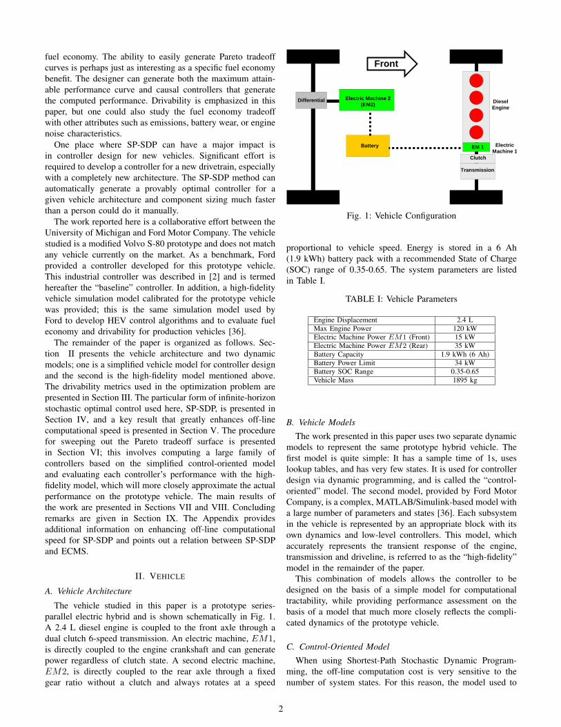
The vehicle studied in this paper is a prototype series-parallel electric hybrid and is shown schematically in Fig. 1.A 2.4 L diesel engine is coupled to the front axle through adual clutch 6-speed transmission. An electric machine, EM1,is directly coupled to the engine crankshaft and can generatepower regardless of clutch state. A second electric machine,EM2, is directly coupled to the rear axle through a fixedgear ratio without a clutch and always rotates at a speed

tex t

tex t

Differential

Battery

Electric Machine 2(EM2)

t etex t

Transmission

EM 1

Clutch

Front

Electric Machine 1

Diesel Engine

Fig. 1: Vehicle Configuration

proportional to vehicle speed. Energy is stored in a 6 Ah(1.9 kWh) battery pack with a recommended State of Charge(SOC) range of 0.35-0.65. The system parameters are listedin Table I.

TABLE I: Vehicle Parameters

Engine Displacement 2.4 LMax Engine Power 120 kWElectric Machine Power EM1 (Front) 15 kWElectric Machine Power EM2 (Rear) 35 kWBattery Capacity 1.9 kWh (6 Ah)Battery Power Limit 34 kWBattery SOC Range 0.35-0.65Vehicle Mass 1895 kg

B. Vehicle Models

The work presented in this paper uses two separate dynamicmodels to represent the same prototype hybrid vehicle. Thefirst model is quite simple: It has a sample time of 1s, useslookup tables, and has very few states. It is used for controllerdesign via dynamic programming, and is called the “control-oriented” model. The second model, provided by Ford MotorCompany, is a complex, MATLAB/Simulink-based model witha large number of parameters and states [36]. Each subsystemin the vehicle is represented by an appropriate block with itsown dynamics and low-level controllers. This model, whichaccurately represents the transient response of the engine,transmission and driveline, is referred to as the “high-fidelity”model in the remainder of the paper.

This combination of models allows the controller to bedesigned on the basis of a simple model for computationaltractability, while providing performance assessment on thebasis of a model that much more closely reflects the compli-cated dynamics of the prototype vehicle.

C. Control-Oriented Model

When using Shortest-Path Stochastic Dynamic Program-ming, the off-line computation cost is very sensitive to thenumber of system states. For this reason, the model used to

2

develop the controller must be as simple as possible. Thevehicle model used here contains the minimum functionalityrequired to model the vehicle behavior of interest on a second-by-second basis. Dynamics much faster than the sample timeof 1s are ignored. Long-term transients that only weaklyaffect performance are also ignored; coolant temperature isone example.

The vehicle hardware allows three main operating condi-tions:

1) Parallel Mode-The engine is on and the clutch isengaged.

2) Series Mode-The engine is on and the clutch is disen-gaged. The only torque to the wheels is through EM2.

3) Electric Mode-The engine is off and the clutch isdisengaged; again the only torque to the wheels isthrough EM2.

The model does not restrict the direction of power flow. Theelectric machines can be either motors or generators in allmodes.

The dynamics of the internal combustion engine are ig-nored; it is assumed that the engine torque exactly matchesvalid commands and the fuel consumption is a function onlyof speed, ωICE , and torque, TICE . The fuel consumption mf

is derived from a lookup table based on dynamometer testing,

mf = F (ωICE , TICE).

The dual clutch transmission has discrete gears and notorque converter. The transmission is modeled with a constantmechanical efficiency ηtrans. Gear shifts are allowed everytime step and transmission dynamics are assumed negligible.While the physical configuration of the transmission allowsarbitrary shifting, the low-level transmission controller en-forces sequential up/down shifting and the model respects thisassumption. This technique is advantageous in hardware be-cause shifts execute by smoothly transitioning between the twoclutches and continually transmitting torque. One transmissionshaft holds the even gears and the other the odd gears. Anarbitrary gear may be selected when the clutch is disengaged.When the clutch is engaged, the vehicle is in parallel modeand the engine speed is assumed directly proportional to wheelspeed based on the current gear ratio Rg ,

ωICE = Rgωwheel.

The electric machine EM1 is directly coupled to thecrankshaft, and thus rotates at the engine speed ωICE ,

ωEM1 = ωICE .

In parallel mode, when providing power to the wheels, thetorques TICE and TEM1 are proportional to wheel torquebased on the current gear ratio Rg and ηtrans; during re-generative braking, for example, when absorbing power fromthe wheels1, the torques are proportional based on Rg and1/ηtrans. Similarly, the rear electric machine torque TEM2

is proportional to the machine’s gear ratio REM2 and reardifferential efficiency ηdiff when providing power, and is

1Note that the model accounts for power loss in both directions.

proportional to REM2 and 1/ηdiff when absorbing power.The total wheel torque Twheel from both axles is thus the sumof the ICE and EM1 torques to the wheel and the rear electricmachine EM2 torque to the wheel, namely

Rgτtrans(TICE + TEM1) +REM2τdiff (TEM2) = Twheel,(1)

where

τtrans(T ) =

{ηtransT if T ≥ 0Tη trans

otherwise,

and similarly for τdiff .The clutch can be disengaged at any time, and power is

delivered to the road through the rear electric machine EM2.This condition is treated as the neutral gear 0, which combineswith the 6 standard gears for a total of 7 gear states. If theengine is on with the clutch disengaged, the vehicle is in seriesmode. The engine-EM1 combination acts as a generator andcan operate at an arbitrary torque and speed. If the engine isoff while the clutch is disengaged, the vehicle is in electricmode. The clutch is never engaged with the engine off, sothis mode is undefined and not used.

The battery system is similarly reduced to table lookupform. The electrical dynamics due to the motor, battery, andpower electronics are assumed sufficiently fast to be ignored.The energy losses and efficiencies in these components canbe grouped together such that the change in battery SOC isa function κ of electric machine speeds ωEM1 and ωEM2,torques TEM1 and TEM2, and battery SOC at the current timestep,

SOCk+1 = κ(SOCk, ωEM1k, ωEM2k

, TEM1k, TEM2k

). (2)

In this simplest configuration, assuming a known vehiclespeed, the only state variable required for the vehicle modelis the battery SOC. Changes in battery performance due totemperature, age, and wear are ignored. Additional states arerequired to represent the stochastic drive cycle and to trackdrivability metrics.

During operation, the desired wheel torque is defined by thedriver. If we assume the vehicle must meet the torque demandperfectly, then the sum of the ICE and EM contributions towheel torque (1) must equal the demanded torque Tdemand,

Twheel = Tdemand.

This adds a constraint to the control optimization, reducing the4 control inputs to a 3 degree-of-freedom problem. In parallelmode, the control inputs are Engine Torque, EM1 Torque, andGear. In series mode, the electric machine command becomesEM1 Speed.

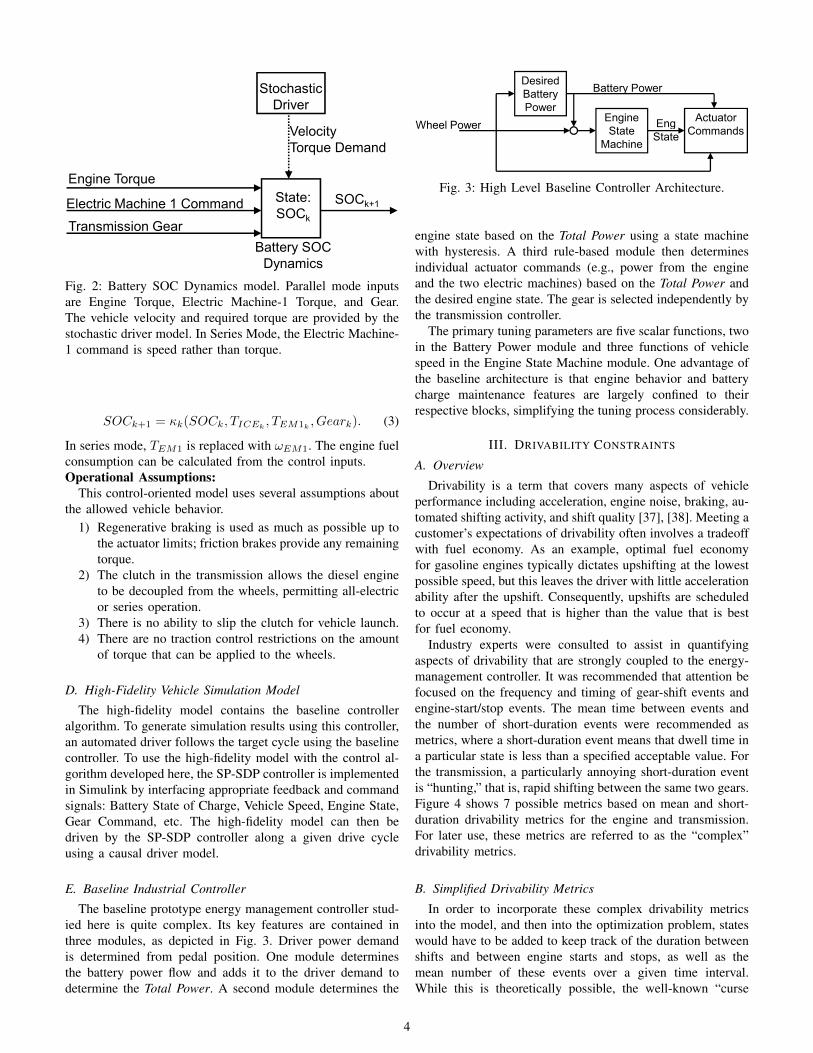
Optimization using the control-oriented model assumes aperfect driver during the design process; specifically, thedesired road power is calculated as the exact power requiredto drive the cycle at that time. A PID controller based onvelocity feedback is used to represent a causal driver duringsimulation of the high-fidelity model. Now, given vehiclespeed, demanded road power and this choice of control inputs,the dynamics become an explicit function κk of the stateBattery SOC and the three control choices shown in Fig. 2,

3

Stochastic

State:

SOCk

Velocity

Torque Demand

Battery SOC

Dynamics

Engine Torque

SOCk+1

Stochastic

Driver

Electric Machine 1 Command

Transmission Gear

Fig. 2: Battery SOC Dynamics model. Parallel mode inputsare Engine Torque, Electric Machine-1 Torque, and Gear.The vehicle velocity and required torque are provided by thestochastic driver model. In Series Mode, the Electric Machine-1 command is speed rather than torque.

SOCk+1 = κk(SOCk, TICEk, TEM1k

, Geark). (3)

In series mode, TEM1 is replaced with ωEM1. The engine fuelconsumption can be calculated from the control inputs.Operational Assumptions:

This control-oriented model uses several assumptions aboutthe allowed vehicle behavior.

1) Regenerative braking is used as much as possible up tothe actuator limits; friction brakes provide any remainingtorque.

2) The clutch in the transmission allows the diesel engineto be decoupled from the wheels, permitting all-electricor series operation.

3) There is no ability to slip the clutch for vehicle launch.4) There are no traction control restrictions on the amount

of torque that can be applied to the wheels.

D. High-Fidelity Vehicle Simulation Model

The high-fidelity model contains the baseline controlleralgorithm. To generate simulation results using this controller,an automated driver follows the target cycle using the baselinecontroller. To use the high-fidelity model with the control al-gorithm developed here, the SP-SDP controller is implementedin Simulink by interfacing appropriate feedback and commandsignals: Battery State of Charge, Vehicle Speed, Engine State,Gear Command, etc. The high-fidelity model can then bedriven by the SP-SDP controller along a given drive cycleusing a causal driver model.

E. Baseline Industrial Controller

The baseline prototype energy management controller stud-ied here is quite complex. Its key features are contained inthree modules, as depicted in Fig. 3. Driver power demandis determined from pedal position. One module determinesthe battery power flow and adds it to the driver demand todetermine the Total Power. A second module determines the

Desired

Battery

PowerEngine

State

Actuator

CommandsWheel Power

Battery Power

Eng State

Machine

CommandsWheel Power Eng

State

Fig. 3: High Level Baseline Controller Architecture.

engine state based on the Total Power using a state machinewith hysteresis. A third rule-based module then determinesindividual actuator commands (e.g., power from the engineand the two electric machines) based on the Total Power andthe desired engine state. The gear is selected independently bythe transmission controller.

The primary tuning parameters are five scalar functions, twoin the Battery Power module and three functions of vehiclespeed in the Engine State Machine module. One advantage ofthe baseline architecture is that engine behavior and batterycharge maintenance features are largely confined to theirrespective blocks, simplifying the tuning process considerably.

III. DRIVABILITY CONSTRAINTS

A. Overview

Drivability is a term that covers many aspects of vehicleperformance including acceleration, engine noise, braking, au-tomated shifting activity, and shift quality [37], [38]. Meeting acustomer’s expectations of drivability often involves a tradeoffwith fuel economy. As an example, optimal fuel economyfor gasoline engines typically dictates upshifting at the lowestpossible speed, but this leaves the driver with little accelerationability after the upshift. Consequently, upshifts are scheduledto occur at a speed that is higher than the value that is bestfor fuel economy.

Industry experts were consulted to assist in quantifyingaspects of drivability that are strongly coupled to the energy-management controller. It was recommended that attention befocused on the frequency and timing of gear-shift events andengine-start/stop events. The mean time between events andthe number of short-duration events were recommended asmetrics, where a short-duration event means that dwell time ina particular state is less than a specified acceptable value. Forthe transmission, a particularly annoying short-duration eventis “hunting,” that is, rapid shifting between the same two gears.Figure 4 shows 7 possible metrics based on mean and short-duration drivability metrics for the engine and transmission.For later use, these metrics are referred to as the “complex”drivability metrics.

B. Simplified Drivability Metrics

In order to incorporate these complex drivability metricsinto the model, and then into the optimization problem, stateswould have to be added to keep track of the duration betweenshifts and between engine starts and stops, as well as themean number of these events over a given time interval.While this is theoretically possible, the well-known “curse

4

Gear Hunting EventsEngine Off Dwell Time <X seconds

Gear Dwell Time < X secondsEngine On Dwell Time < X secondsShort Duration Events

Mean Engine Off Time

Mean Time in GearMean Engine On TimeMean Dwell Times

Transmission BehaviorEngine Behavior

Gear EventsEngine EventsSimplified Metrics

Fig. 4: Drivability Metric Reduction. The seven complexengine and transmission metrics are divided into two cat-egories, mean dwell times and short-duration dwell times.These metrics are then reduced to the two simplified metrics.

of dimensionality” would render the associated stochasticoptimization problem computationally intractable. Even if theoptimization problem could be solved, the designer would befaced with the difficult job of assigning relative weights toeach of the metrics when performing a tradeoff analysis.

We chose therefore to simplify these complex metrics intotwo measures of drivability that can be more easily used. Thefirst drivability metric is termed gear events, and is defined tobe the total number of shift events on a given trip. The seconddrivability metric is termed engine events, and is defined to bethe total number of engine start and stop events on a trip. Bydefinition, engine starts and stops are each counted as an event.Each shift with the clutch engaged is counted as a gear event,whereas engaging or disengaging the clutch is not counted asa gear event, regardless of the gear before or after the event.

Figure 5 shows that the complex and simple metrics arestrongly correlated; specifically, the figure shows that reducingthe total number of engine on-off events over a drive cyclereduces the occurrence of events where the engine is on forless than 3, 5, 10 or 30 seconds. The data are shown alongwith a straight-line least-squares fit. The other complex metricslisted in Fig. 4 show similar correlations, being approximatelymonotone functions of the simple metrics. The data in Fig.5 were obtained by simulating the SP-SDP controllers of theensuing sections on the high-fidelity model. The results arepresented here in order to motivate the use of the simplifiedmetrics in the rest of the paper.

C. Inclusion of Drivability Constraints in the Cost Function

The first step in the design of a controller with acceptabledrivability properties is to pose a cost function that permitsa compromise between fuel economy and drivability. This isachieved by the use of penalties. Specifically, the cost functionover a particular drive cycle (suppressing the summing index)is

J =

T∑0

mf + α

T∑0

IGE(x, u) + β

T∑0

IEE(x, u),

where I(x, u) are indicator functions and thus equal one whena state and control combination produces a gear event (GE)or engine event (EE) as defined in Section III-B, and are zerootherwise. T is the total trip time, from key-on to key-off. Thedrivability behavior is not incorporated as a direct constraint,

0 20 40 60 80 100 1200

10

20

30

40

50

60

70

Engine Events

Occ

uren

ces

≤ 3 s≤ 5 s≤ 10 s≤ 30 s

Fig. 5: Engine on durations less than some number of secondscompared to the simplified engine events metric. Data areshown for cutoffs of 3, 5, 10, and 30 seconds.

so the search for the weighting factors α and β involvessome trial and error because the mapping from penalty tooutcome is not known a priori. Note that setting α and β tozero corresponds to solving for optimal fuel economy withoutregard to drivability.

Controllers based only on fuel economy and drivabilitycompletely drain the battery as they seek to minimize fuel. Anadditional cost is added to ensure that the vehicle is chargesustaining over the cycle. This SOC-based cost only occurs atthe terminal state, xT (that is, at the end of the trip at key-off),and is represented as a function φSOC(xT ). The performanceindex for a particular drive cycle is then

J =

T∑0

mf+α

T∑0

IGE(x, u)+β

T∑0

IEE(x, u)+φSOC(xT ).

(4)

IV. SHORTEST PATH STOCHASTIC DYNAMICPROGRAMMING

A. Problem FormulationAs the cycle is not known exactly in advance, this opti-

mization is conducted in the stochastic sense by minimizingthe expected sum of a running cost function c(xk, uk, wk),where xk is the state, uk is a particular control choice in theset of allowable controls U(xk), and wk is a random variablearising from the unknown drive cycle. The expectation over therandom process w is denoted Ew. The optimization problemis

minEw∞∑k=0

c(xk, uk, wk) (5)

subject to the system dynamics,xk+1 = f(xk, uk, wk) (6)

with uk ∈ U(xk), where

U(xk) = {uk | g1(xk, uk) ≤ 0, g2(xk, uk) = 0 }.

5

Actuator limits, torque delivery requirements, and other systemrequirements are incorporated in the constraints g1 and g2,which are enforced at each time step, in contrast to drivabilitygoals, which involve performance over the whole cycle.

To implement the optimization goal (5), the running costfunction is prescribed to represent (4),

c(x, u, w) = mf (x, u)+αIGE(x, u)+βIEE(x, u)+φSOC(x,w).(7)

The SOC-based cost φSOC(x,w) applies only at the endof the trip, when the key-off event occurs. As explained inSection IV-D, the transition to key-off is captured by thestochastic drive-cycle model in the random process w. Thecost φSOC(x,w) at the key-off event replaces the terminal-time cost φSOC(xT ) in (4).

B. Bellman Equation

To determine the optimal control strategy for this vehi-cle, the SP-SDP algorithm is used [25], [26], [33], [34].This method directly generates a causal, time-invariant, state-feedback controller. Characteristics of future driving behaviorare specified via a finite-state Markov chain rather than exactfuture knowledge. Given the system model (6), the optimalcost V ∗(x) over an infinite horizon is a function of the statex and satisfies

V ∗(x) = minu∈U(x)

Ew[c(x, u, w) + V ∗(f(x, u, w))], (8)

where c(x, u, w) is the instantaneous cost as a function of stateand control; (7) is a typical example. This equation representsa compromise between minimizing the current cost c(x, u, w)and the expected future cost V (f(x, u, w)). The control uis selected based on the expectation over w, rather than adeterministic cost, because the future can only be estimatedbased on the probability distribution of w. Note that the costV (x) is a function of the state only. This cost is finite for allx if every point in the state space has a positive probabilityof eventually transitioning to an absorbing state that incurszero cost from that time onward. Here, the absorbing state iskey-off, the end of the drive cycle.

The optimal control u∗ is any control that achieves theminimum cost V ∗(x)

u∗(x) = argminu∈U(x)

Ew[c(x, u, w) + V ∗(f(x, u, w))]. (9)

Remark: At each time step k, random variable wk in (8) and(9) may be conditioned on the state and control input,

P (wk|xk, uk). (10)

C. Stochastic Drive-Cycle Model

The drive cycle is modeled as a Markov chain. The drivecycle is assigned two states: current velocity vk and currentacceleration ak, which are included in the full system state xk.The random variable wk in (8) is the acceleration at the nexttime step. Specifying the drive cycle is equivalent to assigninga probability distribution to w, that is, specifying

P (ak+1|vk, ak) (11)

for pairs vk, ak. Following [25], the transition probabilities(11) are estimated from known drive cycles that representtypical behavior, referred to as “design cycles.” The variablesvk, ak, and ak+1 are discretized to form a grid. For eachdiscrete state [vk,ak] there are a variety of outcomes ak+1.The probability of each outcome ak+1 is estimated basedon its frequency of occurrence during the design cycle, andis clearly a function of the state as in (10); see [25], [26]for more detail. Specific design cycles include the standardcycles used to establish “window sticker” fuel economy suchas the Federal Test Procedure (FTP). As mentioned previously,design cycles might also include measured driving behaviorover “real world” vehicle use.

Bringing this all together, the full system state vector xcontains five components: one state for the vehicle (BatterySOC), two states for the stochastic driver (vk, ak), and twostates to study drivability (Gear and Engine State). Thisformulation is termed the “SP-SDP-Drivability” controller. Asummary of system states is shown in Table II.

TABLE II: Vehicle and Driver Model States, SP-SDP Driv-ability Controller

State UnitsBattery Charge (SOC) unitless

Vehicle Speed m/sVehicle Acceleration m/s2

Gear Integer 0-6Engine State On or Off

The inputs to the model are engine torque, gear number, andthe powers or torques of the two electric machines. Lookingahead, Section V shows how an off-line optimization step canbe used to replace the two electric machines by a single inputrepresenting total electric machine power, thereby reducingthe inputs for the optimization problem to engine torque, gearnumber, and total electric machine power. The power balanceto meet driver demand given in (1) then allows the eliminationof one more input. The final control input u that will be used inthe optimization problem consists therefore of Engine Torqueand Gear.Remarks: (a) The form of the Bellman equation (8) associatedwith any dynamic programming problem allows an analyticalcomparison with ECMS and is discussed in Section D ofthe Appendix. (b) As demands on controller functionalitygrow, so also must the complexity of the design model. Forexample, to study fuel economy using deterministic dynamicprogramming, the only state required is the battery state ofcharge; the control inputs are Engine Torque and Gear. Twomore states are required to study the stochastic version, and thesimplified drivability model used here requires two additionalstates.

D. Terminal State

As mentioned in Section IV-B, the dynamics of the systemmust contain an absorbing state. For this case, the absorbingstate represents key-off, when the driver has finished the trip,

6

0.35 0.4 0.45 0.5 0.55 0.6 0.65200

400

600

800

1000

1200

1400

1600

SOC

Val

ue F

unct

ion

Velocity = 0 m/sVelocity = 8.6 m/sVelocity = 12.7 m/sVelocity = 25.3 m/s

Stopped

Highway Speed

Fig. 6: Value Function V (x) for several velocities and fixedacceleration. The quadratic penalty on SOC strongly affectsthe value function at low speeds when the driver is more likelyto turn the key off and end the trip.

shut down the vehicle, and removed the key. Once the key-off event occurs, there are no further costs incurred, the tripis over, and the vehicle cannot be restarted. The probabilityof transitioning to this state is zero unless the vehicle iscompletely stopped (vk, ak = 0). The probability of a tripending once the vehicle is stopped is calculated based onthe design cycles. This probability is less than one because astopped vehicle could represent a traffic light or other typicaldriving event that does not correspond to the end of a trip.

For fuel economy certification, the battery final SOC mustbe close to the initial SOC. To include this in the SP-SDPformulation, a cost is imposed when the vehicle transitionsinto the key-off state and the SOC is less than the initial SOC.This penalty accrues only once, so the absorbing state has zerocost from then onwards. Here we add a quadratic penalty inSOC if the final SOC is less than the initial SOC. No penaltyis assigned if the final SOC is higher than the initial SOC.

The effects of this key-off penalty are clearly visible inthe value function V (x). For the fuel-only case, the valuefunction depends on the current acceleration, velocity, andSOC. Fig. 6 shows V (x) as a function of SOC for oneparticular acceleration and several velocities, with target finalSOC equal to 0.5. Notice that at low velocities, the valuefunction has a pronounced quadratic shape for SOC under0.5, but it flattens out at higher speeds. The SOC penalty onlyoccurs at key-off, which can only occur at zero speed. Thusthe SOC key-off penalty strongly affects the value function atlow speeds, when there is a higher probability of key-off inthe near future. At higher speeds, there is little chance of key-off anytime soon, so the SOC penalty only weakly affects thevalue function. Moreover, there will be a deceleration phasebefore reaching zero speed and thus an opportunity to rechargethe battery.

E. Implementable Constraints

Stochastic Dynamic Programming is inherently computa-tionally intensive and can quickly become intractable. Thecomputational burden is exponential in the number of systemstates; thus the cost function (7) should depend on a minimalnumber of states.

For optimization, at each time step a penalty is assignedif either a shift or engine event occurs. The two additionalstates required to implement this cost function are the currentgear and the engine state. Thus, including drivability in theoptimization imposes roughly a factor of ten increase incomputation over the fuel-only case.

In contrast, suppose the metric of interest were based on amoving window in time. The number of required grid pointsscales with the number of time steps used to specify themetric. For the 1 second update time studied here, penalizingengine events of 5 seconds duration or less (rather than thesimple on/off used here) would require 5 grid points forthe time history, increasing the size of the state-space by acorresponding factor of 5 over the on/off case.

V. COMPUTATION REDUCTION

A. Theory

Proposition: (Minimization Decomposition)Consider a Bellman equation of the form

V ∗(x) = minu∈U(x),u∈U(x,u)

Ew[c(x, u, u, w) + V ∗(f(x, u, w))],

(12)and define

c(x, u) = minu∈U(x,u)

Ew[c(x, u, u, w)]. (13)

Then V ∗(x) satisfies (12) if, and only if, it satisfies

V ∗(x) = minu∈U(x)

Ew[c(x, u) + V ∗(f(x, u, w))].� (14)

The proof and more detail are available in the Appendix.This result allows a significant reduction in computationalcomplexity for problems that have the specific structure (12).The reduced Bellman equation (14) may be solved using onlythe reduced control space U(x). This structure appears quiteoften in energy management problems (see Appendix).

The above decomposition has been exploited in previouswork without explicit theoretical justification [16], [39]. Atypical example is the power-split HEV configuration whichuses engine power and speed as inputs without an enginespeed state [39]. The fuel-minimizing engine speed (u) foreach engine power (u) is precomputed and stored as a table(see Appendix).

The following subsection details the physical explanation ofthe structure (12) for the vehicle considered in this work andhow the decomposition is implemented.

B. Super Electric Machine

In comparison to previous work in [1], the addition ofa second electric machine makes the computation of a SP-SDP solution more complex by forcing the algorithm to

7

consider an additional dimension in the control space. If theadditional control variable is discretized with say N = 10points, the size of the minimization operation in (8) over pairs(x, u) increases by a factor of ten. Exploiting the structurerepresented by (12) and using Minimization Decompositionreduces the computational cost to that of a vehicle with asingle electric machine, i.e., a 90% reduction. The addition ofthe second electric machine is then approximately free in termsof computing an off-line solution to the SP-SDP problem.

Intuitively, Minimization Decomposition lumps the twoelectric machines into a single “Super Electric Machine.”This device is a black box that takes a desired wheel-torquecommand as an input and uses the vehicle velocity, enginetorque, and gear to achieve the desired torque with minimalelectric power, as shown in Fig. 7. The required minimizationis static, and in an off-line setting such as SP-SDP, can be doneonce and reused. Once the static optimization is performed,the Super Electric Machine appears as a single power sourcefor the SP-SDP optimization. Internally, however, the SuperElectric Machine optimizes between the two (or possiblymore) electric machines and issues appropriate commands.

A more technical justification follows. The torque balance(1) allows a tradeoff between the two electric machine torques.The system dynamics are only affected by the net change inSOC

u : δSOC (15)

and not by the split of the electric machine torques, which canbe defined by one command

u : TEM2. (16)

For a given TEM2, velocity, and gear, TEM1 is exactlydetermined by δSOC. Since the power-split optimization isstatic (i.e., independent of the dynamic states of the model,including SOC), it takes the form (12) and can be computeda priori using (13) without loss of optimality. This reducesthe dimension of the control space by one. The fundamentalassumption that allows this to work is that the electric machinebehaviors depend only on the current values of the EM torquecommands, current gear, and velocity, and in particular, do notdepend on their past values. For any control command underconsideration, the knowledge of current gear, velocity, TEM2,δSOC, and the required wheel torque uniquely determinesall the terms in the torque balance (1). An optimal u canthen be selected as in (13). The required engine torque isdetermined from the torque balance, accounting for for thedirection-dependent efficiency losses in the transmission.

The physical control inputs to the system are engine torque,gear, EM1 torque and EM2 torque. The constraint to matchdriver demand torque removes one degree-of-freedom. Byreplacing the two electric machine commands with a singleelectric wheel torque command, the SP-SDP algorithm hasonly 2 control inputs.

VI. SIMULATION PROCEDURE

SP-SDP-based controllers are compared to a baseline in-dustrial controller. SP-SDP controllers are designed using thecontrol-oriented model and evaluated using the high-fidelity

Gear

Total Wheel TorqueElectric Wheel

Torque Command

Super Electric Machine

EM-S

Mechanical Analog:

Internal Function:

Optimize

EM1

Gear

Velocity

Engine Torque

EM2

Super Electric Machine

Electric Wheel

Torque Command

+

+

Total Wheel Torque

Fig. 7: Schematic diagram of a conceptual “Super ElectricMachine” that optimizes the mix between the two electricmachines. This allows one degree of freedom of the controloptimization to be carried out off-line while maintaining theoptimality of the solution.

0 200 400 600 800 1000 1200 1400 1600 1800 20000

10

20

30

40

50

60FTP

time (s)

Spe

ed (

mph

)

0 200 400 600 800 1000 12000

20

40

60

80

time (s)

Spe

ed (

mph

)

NEDC

Fig. 8: Federal Test Procedure (FTP) and New European DriveCycle (NEDC).

vehicle simulation model of Section II-D. This demonstratessome robustness by using two models of the same vehicle,differing in the level of detail in their dynamics. Strictlyspeaking, the optimality guarantees are no longer valid be-cause the test model is different from the design model. Forpractical purposes, a strictly optimal model-based controlleris unattainable in hardware because a model will always havesome mismatch with a real vehicle. Demonstrating excellentperformance on the (exact) design model is only marginallyuseful as it presents no model uncertainty. By designing thecontroller on a simple model and testing on a (not perfectlymatched) complex model, we more closely approximate theprocess of designing on the basis of a model and testing onhardware.

8

Both SP-SDP and the baseline controllers are simulated ontwo government test cycles, the US Federal Test Procedure andthe New European Drive Cycle (NEDC), which are shown inFig. 8. Procedurally, this is conducted as follows:

1) A family of SP-SDP controllers is designed accordingto the methods of Section IV. A family is generated byfixing the model driving statistics and sweeping the 2drivability penalties α and β in (7).

2) Each controller in the family is simulated on the high-fidelity model using a causal driver, thus accountingfor all the dynamics and real vehicle characteristicsneglected in the optimization.

3) The fuel economy and drivability metrics are recorded.Fuel economy is computed in units of MPG (Milesdriven Per Gallon of fuel consumed), and hence largernumbers mean better fuel economy.

In the end, each family contains a few hundred individualcontrollers which have each been simulated on the cycle inquestion. Each simulation yields a data point with associatedfuel economy and drivability metrics. Each controller in thefamily has different drivability and fuel economy characteris-tics because of the varying drivability penalties.

Because the simulations on the high-fidelity model use acausal driver model, the final SOC is not guaranteed to exactlymatch the starting SOC. This could yield false fuel economyresults, so all fuel economy estimates are corrected based onthe final SOC of the drive cycle. This is done by estimatingthe additional fuel required to charge the battery to its initialSOC, or the potential fuel savings shown by a final SOC thatis higher than the starting level. This correction is appliedaccording to

∆mf = CBatt∆SOCBSFCmin

ηRegenmax

(17)

where ∆mf is the adjustment to the fuel used, CBatt isthe battery capacity, ∆SOC is the difference between thestarting and ending SOC, BSFCmin is the best Brake SpecificFuel Consumption for the engine, and ηRegenmax is the bestcharging efficiency of the electric system. This correction is areasonable approximation but not exact; the exact correctiondepends on the controller and the particular cycle. For theFTP cycle, the mean fuel economy correction for the SOCdeviations presented in Fig. 9e is 1.6%, with a 1.3% standarddeviation. Hence, using this simple correction does not changethe conclusions of the presented results in any substantial way.

Fuel economy numbers in this paper always include theSOC correction. The fuel economy of the baseline controllerrunning the FTP cycle is used as the nominal value fornormalization. Therefore the normalized fuel economy of thebaseline controller on FTP is one.

VII. RESULTS: PERFORMANCE TRENDS

A. Fuel Economy Results

The three metrics of interest in this paper are the numbersof gear and engine events, and the total fuel consumptioncorrected for SOC. The family of controllers generated as

described in Section VI yields the results shown in Fig. 9for the FTP cycle and the NEDC.

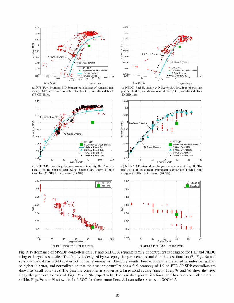
Figs. 9a and 9b show 3-D scatter plots of fuel economyversus gear and engine events for the two cycles. Each pointrepresents a single controller driven on the cycle in question.The total numbers of gear events and engine events areshown on the horizontal axes, while fuel economy is shownon the vertical axis as normalized MPG2. The combinationof these points form a surface in 3-D space depicting thetradeoff surface of various operating conditions. Figure 9ashows a family of controllers designed using FTP statisticsrunning the FTP cycle. Fuel economy data presented in thispaper are normalized to the fuel economy of the baselinecontroller on FTP, shown as a large solid square. Hence, afuel economy greater than one means more miles would betraveled using the same fuel as consumed by the baselinecontroller, or equivalently, less fuel would be consumed forthe same distance traveled. A polynomial surface is fit to theraw data and used to generate isoclines of constant number ofgear events, shown as solid and dashed lines.

Fig. 9c is a 2-D view of Fig. 9a looking along the gear eventsaxis. Each line in the plot represents a constant number of gearevents, while the horizontal and vertical axes show the numberof engine events and normalized fuel economy respectively.This particular vehicle is relatively insensitive to the number ofgear events, so most of the results concentrate on the tradeoffbetween engine activity and fuel economy. The final SOC forthese simulations is shown in Fig. 9e. All simulations start at0.5 SOC.

Similarly, a family of controllers is designed and simulatedon the NEDC. Fuel economy results are again shown in 3-Dand 2-D in Figs. 9b and 9d, while the final SOC is shownin Fig. 9f. Again, fuel economy is normalized to the baselinecontroller performance on FTP, so the baseline controller isslightly less fuel efficient on NEDC (0.99) than FTP (1.00).

B. Discussion

The frontiers of the 2-D and 3-D point clouds in Fig. 9clearly demonstrate the tradeoff between fuel economy anddrivability. The plot of final SOC for the FTP cycle (Fig. 9e)shows a distinct downward trend for large numbers of engineevents. The target final SOC is 0.5, which the controllers comevery close to achieving when engine events are unrestricted(low penalties). The final SOC penalty φSOC(x,w) in (7) usedin the control design process is only applied if the final SOC isbelow this target. For final SOCs above the target, the only costis the fuel spent charging the battery. With smaller numbersof engine events, the controller has less freedom to turn theengine on and charge the battery. In effect, the controllersbecome more conservative and maintain higher SOCs to avoideither additional engine starts or a final SOC that is too low.

An interesting phenomenon occurs when the engine eventspenalty is very high. In this case, to avoid engine shut-down,the only option is to disengage the clutch and enter series

2Recall that more miles per gallon means better fuel economy, while theinverse would hold if units of liters per 100 kilometers were used.

9

0 20 40 60 80 100 120

0100

2003000.75

0.8

0.85

0.9

0.95

1

1.05

1.1

1.15

Engine EventsGear Events

Nor

mal

ized

MP

G

SP−SDPBaseline− 93 Gear Events25 Gear Events75 Gear Events

25 Gear Events

75 Gear Events

(a) FTP: Fuel Economy 3-D Scatterplot. Isoclines of constant gearevents (GE) are shown as solid blue (25 GE) and dashed black(75 GE) lines.

0 10 20 30

050

1000.75

0.8

0.85

0.9

0.95

1

1.05

1.1

1.15

Engine EventsGear Events

Nor

mal

ized

MP

G

SP−SDPBaseline− 19 Gear Events5 Gear Events20 Gear Events

20 Gear Events

5 Gear Events

(b) NEDC: Fuel Economy 3-D Scatterplot. Isoclines of constantgear events (GE) are shown as solid blue (5 GE) and dashed black(20 GE) lines.

0 20 40 60 80 100 1200.75

0.8

0.85

0.9

0.95

1

1.05

1.1

1.15

Engine Events

Nor

mal

ized

MP

G

SP−SDPBaseline− 93 Gear Events25 Gear Event Fit25 Gear Event Data75 Gear Event Fit75 Gear Event Data

75 Gear Events

25 Gear Events

(c) FTP: 2-D view along the gear events axis of Fig. 9a. The dataused to fit the constant gear events isoclines are shown as bluetriangles (25 GE) black squares (75 GE).

0 5 10 15 20 25 300.75

0.8

0.85

0.9

0.95

1

1.05

1.1

1.15

Engine Events

Nor

mal

ized

MP

G

SP−SDPBaseline− 19 Gear Events5 Gear Event Fit5 Gear Event Data20 Gear Event Fit20 Gear Event Data

20 Gear Events

5 Gear Events

(d) NEDC: 2-D view along the gear events axis of Fig. 9b. Thedata used to fit the constant gear event isoclines are shown as bluetriangles (5 GE) black squares (20 GE).

0 20 40 60 80 100 1200.48

0.5

0.52

0.54

0.56

0.58

0.6

0.62

Engine Events

SO

C

SP−SDPBaseline

(e) FTP: Final SOC for the cycle.

0 5 10 15 20 25 300.48

0.5

0.52

0.54

0.56

0.58

0.6

0.62

Engine Events

SO

C

SP−SDPBaseline

(f) NEDC: Final SOC for the cycle.

Fig. 9: Performance of SP-SDP controllers on FTP and NEDC. A separate family of controllers is designed for FTP and NEDCusing each cycle’s statistics. The family is designed by sweeping the parameters α and β in the cost function (7). Figs. 9a and9b show the data as a 3-D scatterplot of fuel economy vs. drivablity events. Fuel economy is presented in miles per gallon,so higher is better, and normalized so that the baseline controller has a fuel economy of 1.0 on FTP. SP-SDP controllers areshown as small dots (red). The baseline controller is shown as a large solid square (green). Figs. 9c and 9d show the viewalong the gear events axes of Figs. 9a and 9b respectively. The raw data points, isoclines, and baseline controller are stillvisible. Figs. 9e and 9f show the final SOC for these controllers. All controllers start with SOC=0.5.

10

mode. With this artifice, it is possible to have a cycle with noother engine events than the initial start and final stop.

The results show some unexpected trends. Figs. 9c and 9dshow a slight decrease in fuel economy for large numbers ofengine events. In some cases on FTP, decreasing the numberof gear events actually increases fuel economy (9c). There aretwo issues here: The optimization is with respect to expectedvalue and not a single sample path as in the plot, and the plotdepicts controller performance on the high-fidelity model andnot the control-oriented design model. To determine whichof these two explanations is the correct one, simulations ofcontroller performance for the FTP cycle were conducted onthe simplified vehicle model (i.e., the control design model)in order to eliminate the issue of model mismatch. Thesesimulations show the same trends discussed above, implyingthat model mismatch is not causing these phenomena. Largenumbers of cycles were then simulated [35] to check theperformance in the expected sense rather than for a singlecycle. This second set of simulations show fuel economy ismonotonic in both gear and engine events as one would expect.

The SP-SDP results show significant (11%) performanceimprovements over the baseline controller for the metricsconsidered here. Production controllers incorporate many ad-ditional attributes, such as noise, harshness, durability, safety,accessory loading, diagnostics, etc. These attributes may de-crease the performance margin when fully incorporated. Oneobvious example is emissions, which was not considered ineither the baseline or SP-SDP controllers. For previous workon NOx emissions, see [40], [23], [41].

VIII. RESULTS: DETAILED PERFORMANCE

A. Results

Several controllers are studied in greater detail on the FTPcycle, which generally yields more interesting behavior thanthe NEDC. The performance of the baseline controller iscompared to 3 SP-SDP controllers in Table III, all runningthe FTP cycle. The SP-SDP controllers are designed usingFTP statistics and are selected from those shown in Figs. 9a,9c, and 9e. SP-SDP #1 is the controller with the best correctedfuel economy without regard to drivability. The peak of thefuel economy surface (Fig. 9a) is very close to the baselinecontroller operating point in terms of drivability. SP-SDP #2has the closest drivability metrics to the baseline controller,and is closely related to SP-SDP #1. SP-SDP #3 is selected byfinding a controller with similar fuel economy to the baselinecontroller and about half the number of drivability events.Essentially, we are presenting two possible design choices:improved fuel economy with similar drivability (SP-SDP#2),or similar fuel economy with reduced drivetrain activity (SP-SDP#3). The designer may also select some compromisebetween the two.

Time histories of the baseline and SP-SDP #1 controllersare presented for the first 500 seconds of the FTP cycle inFig. 10. The engine torque/speed operating points for thesetwo controllers on the full FTP cycle are shown in Fig. 11.

Summary metrics are shown for the baseline and SP-SDPcontrollers in Table IV. The Forward Wheel Energy is the

0 50 100 150 200 250 300 350 400 450 5000

10

20

30

Vel

ocity

(m

/s)

0 50 100 150 200 250 300 350 400 450 5000

100

200

Eng

ine

Tor

que

(Nm

)

0 50 100 150 200 250 300 350 400 450 5000.420.440.460.48

0.50.52

SO

C

0 50 100 150 200 250 300 350 400 450 5000

0.5

1

Eng

ine

Sta

te

time (s)

BaselineSP−SDP

Fig. 10: Time traces of selected simulation parameters. Thebaseline controller is shown as a solid (red) line, and oneparticular SP-SDP controller that yields the best overall fueleconomy is shown as a dashed (black) line; this is SP-SDP #1in Table III.

integral of all motoring (output) wheel power, the EngineOutput Energy is the total energy delivered at the engineoutput shaft, Engine Brake Specific Fuel Consumption (BSFC)(g/kWh) is the total fuel consumed divided by the total engineoutput energy, and Friction Braking Energy is the energydissipated by the friction brakes.

For the electrical propulsion system, the Electro-MechanicalCharge Energy is the total mechanical energy absorbed bythe electric machines, and the Electro-Mechanical DischargeEnergy is the forward mechanical energy provided by theelectric machines. The Electro-Mechanical Losses are thedifference between the two minus the change in battery energy(due to final SOC) and represent all losses in the electricalsystem including accessory loads. The Round-Trip ElectricalEfficiency is the Discharge Energy plus any net change in SOCdivided by the Charge Energy.

B. Discussion

Figs. 10 and 11 and Table IV lend some insight into theperformance differences between the SP-SDP and baselinecontroller. Table IV shows the SP-SDP controller is moreefficient in its use of the diesel engine. The engine primarilyoperates near a high efficiency point or completely off, andyields a lower average BSFC as shown in Fig. 11. Thehigh-torque operating points are also visible in Fig. 10. Theelectric machines are used more extensively by the SP-SDPcontroller, which allows more efficient ICE utilization andmore efficient overall electrical propulsion. Friction brakingis also minimized by the SP-SDP controller.

IX. CONCLUSIONS

An energy management controller for a prototype parallel-series hybrid electric vehicle has been developed using Short-

11

TABLE III: Selected SP-SDP controller performance

Controller Description Fuel Economy (Corrected) Engine Events Gear Events Final SOC Fuel Economy (Uncorr.)Baseline Controller 1.000 88 93 0.505 0.997

SP-SDP #1-Best Fuel Economy 1.119 88 106 0.504 1.117SP-SDP #2-Similar Drivetrain Activity 1.114 88 93 0.506 1.110

SP-SDP #3-Similar Fuel Economy 1.010 34 36 0.561 0.977

TABLE IV: Selected SP-SDP controller performance

Baseline Controller SP-SDP #1 SP-SDP #2 SP-SDP #3Forward (Motoring) Wheel Energy (kJ) 8731 8580 8578 8579

Engine Output Energy (kJ) 11939 11917 11990 12856Friction Braking Energy (kJ) 254.7 5.5 5.5 5.9

Electro-Mechanical Charge Energy (kJ) 5525 7059 7196 9616Electro-Mechanical Discharge Energy (kJ) 2514 3831 3926 5302

Electro-Mechanical Losses (kJ) 2978 3199 3233 4042Round-Trip Electrical Efficiency (%) 46.1 54.7 55.1 58.0

Engine BSFC (g/kWh) 264.8 237.0 236.9 251.6

219

219 219 21

9

230

230

230

230230

240

240240

240

240240

257

257

257

257

257257

274

274

274274

274

343 343

343

Engine Speed (rpm)

Eng

ine

Tor

que

(Nm

)

0 1000 2000 3000 4000 5000 60000

50

100

150

200

250

300

Fig. 11: Engine Torque-Speed operating points on the FTPcycle. The solid black line represents an operational restriction,which both the SP-SDP and baseline controllers respect. Base-line controller operating points are shown as circles (blue) andSP-SDP controller operating points are shown as diamonds(red). The SP-SDP controller is SP-SDP #1 in Table III andalso shown in Fig. 10. The isoclines show constant brakespecific fuel consumption in g/kWh.

est Path Stochastic Dynamic Programming to optimally per-form the inherent tradeoff between fuel efficiency and driv-ability. The SP-SDP-based controllers minimize the expectedvalue of a cost function, using a statistical description ofexpected driving behavior. Here, the cost was a weighted sumof consumed fuel and drivability penalties based on shift eventsand engine on-off events. By varying the weights, the Paretotradeoff surface of fuel economy versus drivability for the SP-SDP-based controllers was evaluated on a high-fidelity vehiclesimulation model.

The performance of the SP-SDP-based controllers wascompared against an industrial baseline controller. For the

same level of drivability, the SP-SDP-based controllers were11% more fuel efficient than the baseline controller on the FTPcycle and the New European Drive Cycle. The SP-SDP-basedcontrollers were designed for the driving statistics of each ofthe two cycles.

In general, dynamic programming is well known to sufferfrom the “curse of dimensionality,” referring to the exponentialexplosion of problem size with the number of state and controlvariables. The system model addressed here had three powersources, namely, an internal combustion engine and two elec-tric machines. A two-step off-line optimization strategy waspresented that preserved optimality while presenting the SP-SDP algorithm with an equivalent system model that containeda single “super” electric machine. Ultimately, this allowed theSD-SDP algorithm to be run on a desktop PC. A similartwo-step optimization strategy is applicable to other vehicleconfigurations that have multiple actuator degrees of freedom.

While the excellent fuel economy of the SP-SDP controllersis very interesting, we feel a more important observation isthat the SP-SDP design method produces causal controllersthat respect constraints and perform well on (and off [35])standard test cycles. SP-SDP-based controllers can be directlyimplemented in a realistic control environment with littlemanual tuning, as demonstrated on an industrial vehicle modelwhich includes detailed subsystem models, dynamics, delays,and limits.

APPENDIX

A. Proof of Minimization DecompositionEquation (12) may be written as

V ∗(x) = minu∈U(x)

minu∈U(x,u)

Ew[c(x, u, u, w) + V ∗(f(x, u, w))],

(18)and by the linearity of expectation

V ∗(x)

= minu∈U(x)

minu∈U(x,u)

(Ew[c(x, u, u, w)]+Ew[V ∗(f(x, u, w))]).

(19)

12

The expectation of the value function is independent of uyielding

V ∗(x)

= minu∈U(x)

( minu∈U(x,u)

Ew[c(x, u, u, w)]+Ew[V ∗(f(x, u, w))]).

(20)

Using the definition (13), (20) becomes (12). �

B. Related Comments on Minimization Decomposition

To implement the controller developed using MinimizationDecomposition, u must still be determined. It may be precom-puted and stored when calculating (13),

u∗(x, u) = argminu∈U(x,u)

c(x, u, u), (21)

and

c(x, u) = c(x, u, u∗(x, u)) = minu∈U(x,u)

c(x, u, u). (22)

This process reduces the space of control actions by U .The computation scales linearly with the number of possiblecontrol actions, and can be significantly reduced depending onthe problem structure and the size of u.

Minimization Decomposition may also be used when solv-ing for non-stationary value functions by appropriately replac-ing V (x) with a time-dependent Vk(x), for either deterministicor stochastic cases [16].

Remark: (Functional Form to use Minimization Decom-position) Suppose a system has dynamics f(x, u, u, w) thatare independent of some control component u and can bereformulated into a function f , such that

f(x, u, w) = f(x, u, u, w) (23)

with probability 1 (w.p. 1). Then the Bellman equation satisfies(12) and the Minimization Decomposition may be used.

While the property (23) seems quite restrictive, it occurssurprisingly often in the energy management problem. It islikely to occur if the number of control inputs M exceeds thedimension of the state space N , leaving a null control directionas used in [38].

Remark: (State Decomposition) In this energy managementproblem (as in most formulations) the dynamics may clearlybe broken down into two parts

f(x, u, w) =

[fu(x, u)fw(x,w)

](24)

where the deterministic states are the known vehicle dynamicsand the stochastic driver dynamics are independent of thecontrol input.

This allows the control inputs to be studied without theeffect of w, simplifying the verification of condition (23).Whenever the number of actuators exceeds the dimension offu, (23) is likely to hold.

The main point is this: if the number of control inputsexceeds the number of states, the required computation canoften be drastically reduced. Even with discrete states (e.g.gear number) the same techniques may often be used.

C. Power-Split Example

Consider for example the “Power-Split” architecture of theToyota Prius and Ford Escape, with a cost function thatpenalizes fuel use and SOC deviations from nominal to attaincharge sustenance. If one assumes that the dynamics of enginespeed changes are negligible at the timescales for energymanagement, the only vehicle state is SOC, as velocity andacceleration are assigned by the driver (stochastically whenusing SP-SDP). Assuming the vehicle matches driver demandtorque, the system is defined by two inputs. By using specificdefinitions of the system variables, the optimization reduces totwo one-degree-of-freedom problems. A common method is totreat the two control inputs as engine speed and engine power.Suppose instead we choose engine speed ωICE and electricalpower Pelec, a slightly different definition. This allows amajor decoupling of the system dynamics. The evolution ofSOC is now only dependent on Pelec = u and completelyindependent of ωICE = u. The engine speed that results inminimum fuel use for a given Pelec can be calculated off-linebecause it is independent of SOC. This results in engine fuelconsumption as a 1-D function of power c(x, u) = c(x, Pelec),rather than the standard 2-D functions of power and speedc(x, u, u) = c(x, Pelec, ωICE).

D. Comparison of SP-SDP to ECMS for Fuel-only Optimiza-tion

One of the most well known optimization methods forenergy management in HEVs is the “Equivalent ConsumptionMinimization Strategy” (ECMS) [19], [42]. This method op-timizes for fuel economy only, which is equivalent to takingthe running cost in (8) as fuel flow rate, that is, c = mf .ECMS is popular among academics because it requires littlecomputation and seems easy to implement. At each time step,the controller minimizes a function that trades off batteryusage vs. fuel,

u∗k(x) = argminu∈U

[mf (x, u) + λk∆SOC(x, u)]. (25)

The design parameter is the weighting factor λk, whichrepresents the relative value of battery charge in terms of fuel.In actual practice, a real difficulty arises because, unless λkis carefully chosen, the vehicle will not be charge sustaining.The required values for λk are highly cycle dependent andtypically require on-line estimation.

It is now shown for the fuel only case that (8) and (9)of the SP-SDP algorithm yield a form very similar to (25)for the computation of the optimal control, with the addedbenefit that the SP-SDP algorithm automatically adjusts theweighting function. First, note that the state can be takenas x = [SOC, x]′, where x consists of vehicle velocity andacceleration. x is independent of the control input u becausevehicle acceleration is defined by the stochastic driver. Themodel (6) can thus be expressed in the form[

SOCk+1

xk+1

]=

[SOCk + ∆SOC(SOCk, xk, uk)f(xk, wk)

].

(26)

13

Next, let V ∗ be the optimal cost to go function in theBellman equation (8), and define

Q(σ, x) = Ew[V ∗(

[σ

f(x, w)

])]

for an arbitrary SOC σ. Substituting the SOC dynamics (26)for σ, the Bellman equation (8) becomes

V ∗(SOC, x) = minu∈U

[mf (SOC, x, u)+

Q(SOC + ∆SOC(SOC, x, u), x)] . (27)

The running cost c = mf in (8) is not a function of therandom variable w and can be removed from the expectation.From this, the expression for the optimal control becomes

u∗(SOC, x) = argminu∈U

[mf (SOC, x, u)+

Q(SOC + ∆SOC(SOC, x, u), x)] . (28)

Doing a first-order Taylor expansion of Q then yields

u∗(SOC, x) ≈ argminu∈U

[mf (SOC, x, u)+

Q(SOC, x) +∂Q(SOC, x)

∂SOC∆SOC(SOC, x, u)

]. (29)

Recognizing that Q(SOC, x), being independent of u, doesnot affect the minimization, and substituting x = [SOC, x]′

into (29), then yields

u∗(x) ≈ argminu∈U

[mf (x, u) +

∂Q(x)

∂SOC∆SOC(x, u)

]. (30)

It follows that ∂Q(x)∂SOC is equivalent to the weighting factor λ

in (25). The SP-SDP algorithm has the same structure as theECMS method, but the weighting factor is a function of thestate variables, and is automatically updated on-line. There isa variant of ECMS method called Adaptive ECMS (A-ECMS)in which the weighting factor is also allowed to change overtime based on the current driving conditions [19]. A-ECMSis even more similar to the SP-SDP algorithm in that bothmethods have a weighting factor that is updated on-line as afunction of the state.

This relationship is illustrated by again studying the valuefunction V (x) as a function of SOC for fixed accelerationand velocity shown in Fig. 6. The local slope of V (x) in thefigure is closely related to the weighting factor in (30), which,once again, is analogous to λ in (25). Fundamentally, all fuel-minimizing control algorithms must estimate the value of bat-tery charge in terms of fuel and thus have some equivalent tothe weighting factor. It may appear linearly and explicitly as inECMS, or nonlinearly and implicitly as in SP-SDP. All knowninformation is incorporated in the weighting factor: currentstate, plant dynamics, and expected future driver demands.Once this weighting factor is determined, the control problemis a simple static optimization.

A basic difference of the algorithms lies in how theyestimate the value of battery charge in terms of fuel: ECMSuses a value assigned by the designer; A-ECMS estimates avalue based on battery charge and recent history; Deterministic

Dynamic Programming uses exact future knowledge; and SP-SDP uses estimates of cycle statistics. A benefit of dynamicprogramming methods, such as SP-SDP, is that they canoptimally accommodate more complicated objectives, such asthe fuel and drivability metrics studied here.

ACKNOWLEDGMENT

The authors would like to thank the reviewers for their help-ful suggestions to clarify the explanation of the MinimizationDecomposition.

REFERENCES

[1] D. Opila, D. Aswani, R. McGee, J. Cook, and J. Grizzle, “Incorporatingdrivability metrics into optimal energy management strategies for hybridvehicles,” in Proc. IEEE Conference on Decision and Control, 2008, pp.4382–4389.

[2] D. Opila, X. Wang, R. McGee, J. Cook, and J. Grizzle, “Performancecomparison of hybrid vehicle energy management controllers on real-world drive cycle data,” in Proc. American Control Conference, 2009,pp. 4618–4625.

[3] ——, “Fundamental structural limitations of an industrial energy man-agement controller architecture for hybrid vehicles,” in Proc. ASMEDynamic Systems and Control Conference, 2009, pp. 213 –221.

[4] A. Sciarretta and L. Guzzella, “Control of hybrid electric vehicles,” IEEEControl Systems Magazine, vol. 27, no. 2, pp. 60–70, 2007.

[5] S. Barsali, M. Ceraolo, and A. Possenti, “Techniques to control theelectricity generation in a series hybrid electrical vehicle,” IEEE Trans.Energy Convers., vol. 17, no. 2, pp. 260–266, 2002.

[6] S. Barsali, C. Miulli, and A. Possenti, “A control strategy to minimizefuel consumption of series hybrid electric vehicles,” IEEE Trans. EnergyConvers., vol. 19, no. 1, pp. 187–195, 2004.

[7] J.-S. Won, R. Langari, and M. Ehsani, “An energy management andcharge sustaining strategy for a parallel hybrid vehicle with CVT,” IEEETrans. Control Syst. Technol., vol. 13, no. 2, pp. 313–320, 2005.

[8] M. Gokasan, S. Bogosyan, and D. J. Goering, “Sliding mode basedpowertrain control for efficiency improvement in series hybrid-electricvehicles,” IEEE Trans. Power Electron., vol. 21, no. 3, pp. 779–790,2006.

[9] D. Prokhorov, “Training recurrent neurocontrollers for real-time appli-cations,” IEEE Trans. Neural Netw., vol. 18, no. 4, pp. 1003–1015, July2007.

[10] C. Dextreit, F. Assadian, I. Kolmanovsky, J. Mahtani, and K. Burnham,“Hybrid vehicle energy management using game theory,” in Proc., SAEWorld Conference, 2008, Paper no. 2008-01-1317.

[11] R. Langari and J.-S. Won, “Integrated drive cycle analysis for fuzzylogic based energy management in hybrid vehicles,” in Proc. 12th IEEEInternational Conference on Fuzzy Systems, vol. 1, 2003, pp. 290–295.

[12] L. Perez, G. Bossio, D. Moitre, and G. Garcia, “Supervisory control ofan HEV using an inventory control approach,” Latin American AppliedResearch, vol. 36, no. 2, pp. 93–100, 2006.

[13] L. Perez and E. Pilotta, “Optimal power split in a hybrid electric vehicleusing direct transcription of an optimal control problem,” Mathematicsand Computers in Simulation, vol. 79, no. 6, pp. 1959–1970, 2009.

[14] S. Kermani, S. Delprat, T. M. Guerra, and R. Trigui, “Predictive controlfor HEV energy management: experimental results,” in Proc. IEEEVehicle Power and Propulsion Conference, 2009, pp. 364–369.

[15] Q. Gong, Y. Li, and Z.-R. Peng, “Trip-based optimal power managementof plug-in hybrid electric vehicles,” IEEE Trans. Veh. Technol., vol. 57,no. 6, pp. 3393–3401, 2008.

[16] L. Johannesson, M. Asbogard, and B. Egardt, “Assessing the potentialof predictive control for hybrid vehicle powertrains using stochasticdynamic programming,” IEEE Trans. Intell. Transp. Syst., vol. 8, no. 1,pp. 71–83, 2007.

[17] G. Paganelli, S. Delprat, T. Guerra, J. Rimaux, and J. Santin, “Equivalentconsumption minimization strategy for parallel hybrid powertrains,” inProc. IEEE 55th Vehicular Technology Conference, vol. 4, 2002, pp.2076–2081.

[18] A. Sciarretta, M. Back, and L. Guzzella, “Optimal control of parallelhybrid electric vehicles,” IEEE Trans. Control Syst. Technol., vol. 12,no. 3, pp. 352–363, 2004.

14

[19] C. Musardo, G. Rizzoni, and B. Staccia, “A-ECMS: An adaptivealgorithm for hybrid electric vehicle energy management,” in Proc. IEEEConference on Decision and Control, 2005, pp. 1816–1823.

[20] C. Musardo, B. Staccia, S. Midlam-Mohler, Y. Guezennec, and G. Riz-zoni, “Supervisory control for NOx reduction of an HEV with a mixed-mode HCCI/CIDI engine,” in Proc. American Control Conference,vol. 6, 2005, pp. 3877–3881.

[21] S. Delprat, T. M. Guerra, and J. Rimaux, “Optimal control of a parallelpowertrain: from global optimization to real time control strategy,” inProc. IEEE 55th Vehicular Technology Conference, vol. 4, 2002, pp.2082–2088.

[22] S. Delprat, J. Lauber, T. M. Guerra, and J. Rimaux, “Control of a parallelhybrid powertrain: optimal control,” IEEE Trans. Veh. Technol., vol. 53,no. 3, pp. 872–881, 2004.

[23] C.-C. Lin, H. Peng, J. Grizzle, and J.-M. Kang, “Power managementstrategy for a parallel hybrid electric truck,” IEEE Transactions onControl Systems Technology, vol. 11, no. 6, pp. 839–849, 2003.

[24] B. Wu, C.-C. Lin, Z. Filipi, H. Peng, and D. Assanis, “Optimal powermanagement for a hydraulic hybrid delivery truck,” Vehicle SystemDynamics, vol. 42, no. 1-2, pp. 23–40, 2004.

[25] C.-C. Lin, H. Peng, and J. Grizzle, “A stochastic control strategy forhybrid electric vehicles,” in Proc. of the American Control Conference,2004, pp. 4710 – 4715.

[26] E. Tate, J. Grizzle, and H. Peng, “Shortest path stochastic control forhybrid electric vehicles,” International Journal of Robust and NonlinearControl, vol. 18, pp. 1409–1429, 2008.

[27] S. Delprat, T. M. Guerra, and J. Rimaux, “Control strategies for hybridvehicles: optimal control,” in Proc. Vehicular Technology Conference,vol. 3, 2002, pp. 1681–1685.

[28] ——, “Control strategies for hybrid vehicles: synthesis and evaluation,”in Proc. Vehicular Technology Conference, vol. 5, 2003, pp. 3246–3250.

[29] G. Paganelli, T. M. Guerra, S. Delprat, J.-J. Santin, M. Delhom, andE. Combes, “Simulation and assessment of power control strategies fora parallel hybrid car,” Proc. of the Institution of Mechanical Engineers,Part D: Journal of Automobile Engineering, vol. 214, pp. 705–717,2000.

[30] S. Kermani, S. Delprat, R. Trigui, and T. M. Guerra, “Predictive energymanagement of hybrid vehicle,” in Proc. IEEE Vehicle Power andPropulsion Conference, 2008, pp. 1–6.

[31] A. Kleimaier and D. Schroder, “An approach for the online optimizedcontrol of a hybrid powertrain,” in Proc. 7th Int Advanced MotionControl Workshop, 2002, pp. 215–220.

[32] D. P. Bertsekas and J. N. Tsitsiklis, Neuro-Dynamic Programming.Athena Scientific, 1996.

[33] D. Bertsekas, Dynamic Programming and Optimal Control. AthenaScientific, 2005, vol. 1.

[34] ——, Dynamic Programming and Optimal Control. Athena Scientific,2005, vol. 2.

[35] D. Opila, “Incorporating drivability metrics into optimal energy man-agement strategies for hybrid vehicles,” Ph.D. dissertation, Universityof Michigan, 2010.

[36] C. Belton, P. Bennett, P. Burchill, D. Copp, N. Darnton, K. Butts, J. Che,B. Hieb, M. Jennings, and T. Mortimer, “A vehicle model architecturefor vehicle system control design,” in Proc. SAE World Congress &Exhibition, 2003, Paper no. 2003-01-0092.

[37] X. Wei, “Dynamic modeling of a hybrid electric drivetrain for fueleconomy, performance and driveability evaluations,” American Societyof Mechanical Engineers, Dynamic Systems and Control Division (Pub-lication) DSC, vol. 72, no. 1, pp. 443–450, 2003.

[38] P. Pisu, K. Koprubasi, and G. Rizzoni, “Energy management anddrivability control problems for hybrid electric vehicles,” in Proc. IEEEConference on Decision and Control, 2005, pp. 1824–1830.

[39] J. Liu and H. Peng, “Modeling and control of a power-split hybridvehicle,” IEEE Trans. Control Syst. Technol., vol. 16, no. 6, pp. 1242–1251, 2008.

[40] E. D. Tate, J. W. Grizzle, and H. Peng, “SP-SDP for fuel consumptionand tailpipe emissions minimization in an EVT hybrid,” IEEE Trans.Control Syst. Technol., vol. 18, no. 3, pp. 673–687, 2010.

[41] C.-C. Lin, H. Peng, J. Grizzle, J. Liu, and M. Busdiecker, “Controlsystem development for an advanced-technology medium-duty hybridelectric truck,” in Proceedings of the International Truck & Bus Meeting& Exhibition, Ft. Worth, TX, USA, 2003.

[42] G. Paganelli, M. Tateno, A. Brahma, G. Rizzoni, and Y. Guezennec,“Control development for a hybrid-electric sport-utility vehicle: strat-egy, implementation and field test results,” in Proc. American ControlConference, 2001, pp. 5064–5069.

Daniel F. Opila (M ’08) received BS and MSdegrees from the Massachusetts Institute of Technol-ogy, Cambridge, Massachusetts, in 2002 and 2003respectively, and the Ph.D. degree from the Univer-sity of Michigan, Ann Arbor, Michigan, in 2010.

He is a Senior Research and Development En-gineer at Converteam Naval Systems in Pittsburgh,a division of GE Energy Management. Previouslyhe was a Visiting Scholar at Ford Motor Company,a Senior Engineer at Orbital Sciences Corporation,and a Mechanical Engineer at Bose Corporation. He

specializes in optimal control of energy systems, including hybrid vehicles,naval power systems, power converters, and renewables.

Dr. Opila is a member of ASME.

Xiaoyong Wang received the B.S. and M.E. degreesfrom Tsinghua University, Beijing, China, in 1998and 2001, respectively, and the Ph.D. degree fromthe University of California at Los Angeles in 2008.

He is a research engineer with Ford Motor Com-pany, Dearborn, Michigan. His main research in-terests include hybrid vehicle control, powertraincontrol and vehicle electrification technologies.

Dr. Wang is a member of ASME and SAE.

Ryan McGee (M ’11) received the B.S.E.E. andM.Eng E.E. degrees from Cornell University, Ithaca,New York, in 1997 and 1998, respectively, and theM.B.A. degree from the University of Michigan,Ann Arbor, Michigan, in 2004.

He is a Technical Expert in Electrification Re-search and Advanced Engineering at Ford MotorCompany. His research focus is on optimal andintelligent control systems applied to electrified pow-ertrains.

Mr. McGee is a member of SAE.

R. Brent Gillespie received the B.S. degree inmechanical engineering from the University of Cal-ifornia, Davis, in 1986, the M.M. degree in pianoperformance from the San Francisco Conservatoryof Music in 1989, and the M.S. and Ph.D. degrees inmechanical engineering from Stanford University in1992 and 1996, respectively. He is currently with theDepartment of Mechanical Engineering, Universityof Michigan, Ann Arbor. His current research inter-ests include haptic interface and teleoperator control,human motor control, prosthetics, and robot-assisted

rehabilitation after neurological injury.

15

Jeffrey A. Cook (M’84–SM’98–F’02) received theB.S.M.E. degree from The Ohio State University,Columbus, Ohio, in 1973 and the M.S. degreein electronic and computer control systems fromWayne State University, Detroit, Michigan, in 1985.

He is an Adjunct Research Professor and Inter-mittent Lecturer in Electrical Engineering and Com-puter Science, and Intermittent Lecturer in NavalArchitecture and Marine Engineering at the Univer-sity of Michigan, Ann Arbor. From 1976 to 2007he worked at the Ford Motor Company, Scientific

Research Laboratory where he held technical and management positions in theUnited States and Europe. His research interests are in the area of embeddedcontrol systems and software.

Mr. Cook is a member of the ASME. In 2009 he led the IEEE ControlSystems Society Committee on Outreach Curriculum Development Project.

Jessy W. Grizzle (S78M79SM90F97) received theB.S.E.E. degree from Oklahoma State University,Stillwater, in 1979 and the M.S.E. and Ph.D. degreesfrom the University of Texas at Austin, in 1980 and1983, respectively.

He is currently the Jerry W. and Carol L. LevinProfessor of Engineering and a Professor of Elec-trical Engineering and Computer Science at theUniversity of Michigan, Ann Arbor. His research in-terests span theoretical nonlinear control, automotivesystems, biomedical systems, and robotics.

Prof. Grizzle is currently a Senior Editor for the IEEE TRANSACTIONSON AUTOMATIC CONTROL.

16