an enhanced craig–bampton method - cmss laboratorycmss.kaist.ac.kr/cmss/papers/2015 an enhanced...

INTERNATIONAL JOURNAL FOR NUMERICAL METHODS IN ENGINEERINGInt. J. Numer. Meth. Engng 2015; 103:79–93Published online 26 March 2015 in Wiley Online Library (wileyonlinelibrary.com). DOI: 10.1002/nme.4880

An enhanced Craig–Bampton method

Jin-Gyun Kim1 and Phill-Seung Lee2,*,†

1Mechanical Systems Safety Research Division, Korea Institute of Machinery and Materials, 156 Gajeongbuk-ro,Yuseong-gu, Daejeon 305-343, Korea

2Division of Ocean Systems Engineering, Korea Advanced Institute of Science and Technology, 291 Daehak-ro,Yuseong-gu, Daejeon 305-701, Korea

SUMMARY

In this paper, we propose a new component mode synthesis method by enhancing the Craig–Bampton (CB)method. To develop the enhanced CB method, the transformation matrix of the CB method is enhancedconsidering the effect of residual substructural modes and the unknown eigenvalue in the enhanced transfor-mation matrix is approximated by using O’Callahan’s approach in Guyan reduction. Using the newly definedtransformation matrix, original finite element models can be more accurately approximated by reduced mod-els. For this reason, the accuracy of the reduced models is significantly improved with a low additionalcomputational cost. We here present the formulation details of the enhanced CB method and demonstrate itsperformance through several numerical examples. Copyright © 2015 John Wiley & Sons, Ltd.

Received 21 March 2014; Revised 13 November 2014; Accepted 22 December 2014

KEY WORDS: structural dynamics; finite element method; model reduction; component mode synthesis;Craig–Bampton method; dynamic substructuring

1. INTRODUCTION

Reduced-order modeling of large finite element (FE) models is essential in many engineering fieldssuch as ocean, mechanical, and aerospace engineering. Component mode synthesis (CMS) meth-ods have been widely used for FE model reductions in structural dynamics. In the CMS methods,the original large structural FE model is partitioned into smaller substructural FE models con-nected at interface boundary. A small proportion of substructural modes (dominant substructuralmodes) and interface constraint conditions are used to reduce the original structural model. Because,instead of the original large structural model, we handle the reduced model constructed using thesmall substructural models, CMS methods can dramatically reduce the computational cost. Theaccurately approximated reduced models are valuable indeed in structural systems design, systemidentification, and experimentally verified model development.

In the 1960s, based on Hurty and Guyan’s idea [1, 2], Craig and Bampton proposed a CMSmethod referred to as the Craig–Bampton (CB) method [3]. Since then, various related studies havebeen performed to develop robust CMS methods [4–11]. However, the CB method is still the mostpopular and widely used CMS method because of its simplicity and reliability. Reviews of the CMSmethods can be found in [12–14].

Using the localized Lagrange multipliers at free interface boundary, Park and Park developedthe flexibility-based CMS (F-CMS) method [9], in which the accuracy of reduced models isimproved by effectively retaining the contribution of residual substructural modes. The conceptualidea has been employed to construct an enhanced transformation matrix used for estimating relative

*Correspondence to: Phill-Seung Lee, Division of Ocean Systems Engineering, Korea Advanced Institute of Science andTechnology, 291 Daehak-ro, Yuseong-gu, Daejeon 305-701, Korea.

†E-mail: [email protected]

Copyright © 2015 John Wiley & Sons, Ltd.

80 J. G. KIM AND P. S. LEE

eigenvalue errors in the CB method [15]. However, the enhanced transformation matrix contains anunknown eigenvalue, and thus, it is not possible to use the transformation matrix in its present formfor the improvement of the original CB method.

In order to overcome this difficulty, we borrow O’Callahan’s idea, which was originally pro-posed to improve Guyan reduction [16]. That is, the unknown eigenvalue is approximated usingO’Callahan’s approach. As a result, a new enhanced transformation matrix is obtained and, usingit, the enhanced CB method is developed. Compared with the original CB method, the enhancedCB method can provide significantly improved reduced-order models with a low additionalcomputational cost.

In the following sections, we briefly review the original CB method, derive the enhanced CBmethod, and present the performance of the enhanced CB method through various numerical exam-ples: rectangular plate, hyperboloid shell, stiffened plate, and solid ring problems. The numericalresults of the enhanced CB method are compared with the original CB and F-CMS methods.

2. CRAIG–BAMPTON METHOD

In the CB method, global (original) structure is partitioned by Ns substructures as in Figure 1(b).The substructures are connected with a fixed interface at the interface boundary � (Figure 1(c)). Thelinear dynamics equations can be expressed by

Mg Rug CKgug D fg ;

Mg D

�Ms Mc

MTc Mb

�; Kg D

�Ks Kc

KTc Kb

�;

ug D�

usub

�; fg D

�fsfb

�;

(1)

where Mg and Kg are the global mass and stiffness matrices, and ug and fg are global displacementand force vectors. The subscript g denotes the global structure and .R/ D d2. /=dt2 with thetime variable t . The subscripts s; b, and c denote substructures, boundary interface, and couplingmatrices, respectively. Note that Ms and Ks are the block diagonal mass and stiffness matricesof substructures.

The global eigenvalue problem is

Kg.�g/i D �iMg.�g/i ; i D 1; 2; : : : ; Ng ; (2)

where �i and .�g/i are the eigenvalue and eigenvector calculated in the global structure, respec-tively, and Ng is the number of DOFs in the global structure. Note that �i and .�g/i are the squareof the i-th natural frequency .!2i / and the corresponding mode in structural dynamics, respectively.

Using the eigenvectors obtained from Equation (2), the global displacement vector ug isrepresented by

ug D ˆgqg ; (3)

where ˆg and qg are the global eigenvector matrix and its generalized coordinate vector,respectively.

In the CB method, the global displacement vector ug can be defined by

ug D�

usub

�D T0

�qsub

�; T0 D

�ˆs �K�1s Kc

0 Ib

�; (4)

Copyright © 2015 John Wiley & Sons, Ltd. Int. J. Numer. Meth. Engng 2015; 103:79–93DOI: 10.1002/nme

AN ENHANCED CRAIG–BAMPTON METHOD 81

Figure 1. Global and partitioned structural models and interface handling in the Craig–Bampton method. (a)Global (non-partitioned) structure �, (b) substructures �i .i D 1; 2; � � � ; Ns/ and interface boundary � (Ns

denotes the number of substructure and Ns D 2 in this figure), and (c) interface boundary treatment.

in which qs is the generalized coordinate vector for the substructural modes, T0 is the transfor-mation matrix, Ib is an identity matrix for the interface boundary, and ˆs is a block diagonaleigenvector matrix calculated by the substructural eigenvalue problems

hK.k/s � �

.k/i M.k/

s

i.�.k//i D 0; i D 1; 2; : : : ; N .k/

q ; for k D 1; 2; : : : ; Ns; (5)

where N .k/q is the number of deformable modes in the k-th substructure, and �.k/i and .�.k//i are

the substructural eigenvalue and eigenvector, respectively.The substructural displacement vector us can be decomposed into the dominant and residual

modes

us D ˆsqs �K�1s Kcub D�ˆd ˆr

� � qdqr

��K�1s Kcub; (6)



where ˆd and ˆr are the dominant and residual substructural eigenvector matrices, respectively,and qd and qr are the corresponding generalized coordinate vectors. The subscripts d and r denotethe dominant and residual terms, respectively. In general, a small number of the dominant modes isused to reduce the global structure. That is, Nd � Nr , in which Nd and Nr are the numbers of thedominant and residual modes, respectively.

Neglecting the residual modes in Equation (6), the global displacement vector ug is approximatedby the dominant substructural modes

ug � Nug D NT0

�qdub

�; NT0 D

�ˆd �K�1s Kc

0 Ib

�; (7)

where NT0 is the reduced transformation matrix. Using NT0 in Equation (1), we can obtain the reducedequations of motion for the partitioned structure

NMpRNup C NKp Nup D Nfp;

NMp D NTT0 MgNT0; NKp D NTT0 Kg

NT0;

Nup D�

qdub

�; Nfp DNTT0

�fsfb

�;

(8)

where NMp and NKp are the reduced mass and stiffness matrices, respectively, and Nup and Nfp are theapproximated displacement and force vectors, respectively. The subscript p denotes the partitionedstructure and an overbar .N/ denotes the approximated quantities.

From Equation (8), the reduced eigenvalue problem is obtained

NKp. N�p/i DN�i NMp. N�p/i ; i D 1; 2; : : : ; NNp; (9)

in which N�i and . N�p/i are the eigenvalue and eigenvector calculated in the reduced model,respectively, and NNp is the number of DOFs in the reduced model.

Using the eigenvectors obtained from Equation (9), the approximated displacement vector Nup isrepresented by

Nup D N̂ p Nqp; (10)

where N̂ p and Nqp are the eigenvector matrix in the reduced model and the corresponding generalizedcoordinate vector, respectively.

3. ENHANCED CRAIG–BAMPTON METHOD

In the original CB method, to construct the reduced transformation matrix NT0 in Equation (7), theresidual substructural modes are simply truncated without any consideration. However, when theresidual substructural modes are properly considered, the transformation matrix can be constructedmore accurately.

Using Equation (6) in Equation (4), ug can be rewritten as

ug D�

usub

�D T0

24 qd

qrub

35 ; T0 D

�ˆd ˆr �K�1s Kc

0 0 Ib

�: (11)



Using Equation (11) in Equation (1), we obtain the equations of motion for the partitionedstructure �

d2

dt2Mp CKp

�up D fp; (12a)

Mp DTT0 MgT0; Kp D TT0 KgT0; (12b)

d2

dt2Mp CKp D

264Oƒd 0 d2

dt2NMc

0T Oƒrd2

dt2D

d2

dt2NMTc

d2

dt2DT OKb C

d2

dt2OMb

375 ; (12c)

up D

24 qd

qrub

35 ; fp D TT0

�fsfb

�; (12d)

where the component matrices are defined by

Oƒd D ƒd Cd2

dt2Id ; ƒd D ˆ

Td Ksˆd ; Id D ˆ

Td Msˆd ; (13a)

NMc D ˆTd

�Mc �MsK�1s Kc

�; (13b)

Oƒr D ƒr Cd2

dt2Ir ; ƒr D ˆTr Ksˆr ; Ir D ˆTr Msˆr ; (13c)

D D ˆTr��MsK�1s Kc CMc

�; (13d)

OMb DMb CKTc K�1s MsK�1s Kc �MT

c K�1s Kc �KTc K�1s Mc ; (13e)

OKb D Kb �KTc K�1s Kc : (13f)

Note that Equation (12) is the original equations of motion that contain all the substructural modes.Substituting Equation (12c) into Equation (12a) with fp D 0 and considering the second row in

the resulting matrix equation, we obtain

qr D � Oƒ�1

r

�d2

dt2Dub

�: (14)

Substituting Equation (14) into Equation (11), us can be represented by

us D ˆdqd �K�1s Kcub �d2

dt2OFr��MsK�1s Kc CMc

�ub; (15)

Table I. Comparison between the CB and enhanced CB methods.

CB Enhanced CB

Transformation matrix NT0 NT0 C NTr

Reduced mass matrix NMp

NMp C NTTr MgNT0

CNTT0 MgNTr C NTTr Mg

NTr

Reduced stiffness matrix NKpNKp C NTTr Kg NT0CNTT0 Kg NTr C NTTr Kg NTr

Size of the reduced matrices NNp NNp



with

OFr D ˆr Oƒ�1

r ˆTr D ˆr

�ƒr C

d2

dt2Ir

��1ˆTr ; (16)

where OFr represents the residual flexibility of the substructures.We here invoke harmonic response .d2=dt2 D ��/, and then OFr can be approximated as

OFr D ˆr Œƒr � �Ir ��1ˆTr

� ˆrƒ�1r ˆ

Tr C �ˆrƒ

�2r ˆ

Tr D Frs C �Frm;

(17)

where Frs and Frm are the static and dynamic parts of the residual flexibility, respectively.Using Equation (17) in Equation (15) and truncating terms higher than the order of �;us can be

approximated as

us � Nus D ˆdqd �K�1s Kcub C �Frs��MsK�1s Kc CMc

�ub; (18)

in which Frs is indirectly calculated by subtracting the dominant flexibility matrix from the fullflexibility matrix as

Frs D K�1s �ˆdƒ�1d ˆ

Td : (19)

Using Nus defined in Equation (18) instead of us in Equation (4), we finally obtain

ug � Nug D NT1 Nup; NT1 D NT0 C NTr ; (20)

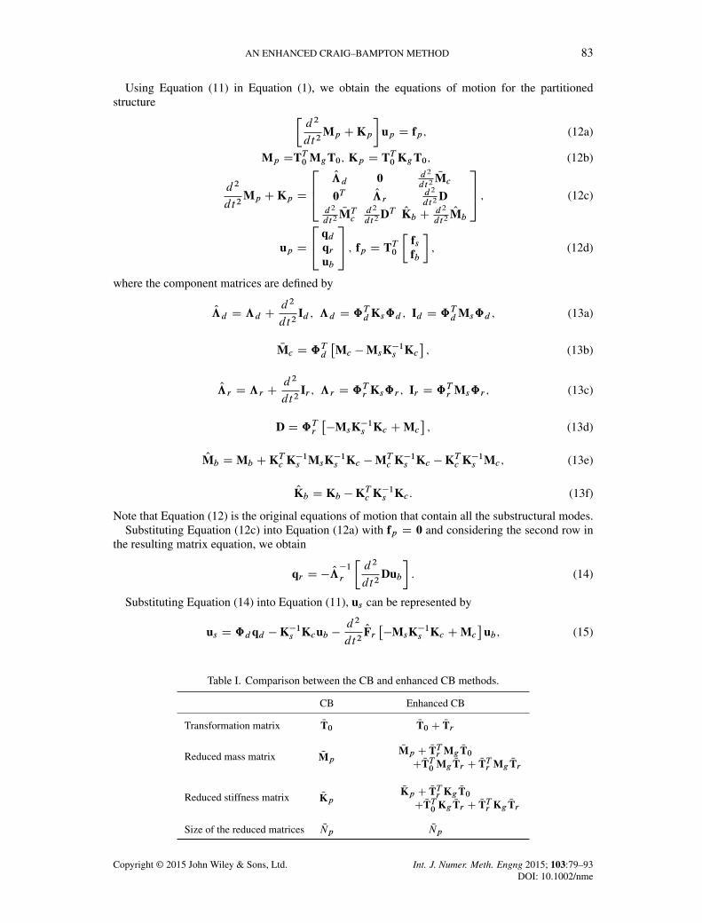
Figure 2. Rectangular plate problem.

Table II. Retained substructural mode numbers N .k/d

in the rectangular plate problem.

CMS Case N.1/d

N.2/d

Nd

CB and enhanced CB 1 7 3 102 13 7 203 26 14 404 52 28 80

F-CMS 1 7 3 102 13 7 203 25 15 404 50 30 80



with

NTr D�

0 �Frs��MsK�1s Kc CMc

�0 0

�; (21)

where NT1 is the transformation matrix enhanced by NTr . Note that, because NTr contains the eigen-value �, it is regarded as a transformation matrix related to the dynamic effect. In the previous study[15], the enhanced transformation matrix NT1 in Equation (20) is employed to develop an accurateerror estimator for the CB method.

Here, a difficulty arises. Because the eigenvalue � in NTr is unknown, the enhanced transformationmatrix NT1 cannot be used to improve the original CB method in its present form. To handle theunknown eigenvalue � in NTr , we employ O’Callahan’s approach, which was proposed to improve

Figure 3. Relative eigenvalue errors in the rectangular plate problem. (a) Nd D 10 and (b) Nd D 20.



Guyan reduction [16]. The excellent performance of O’Callahan’s approach in Guyan reduction hasbeen well known [17, 18]. From Equation (8) with Nfp D 0 and RNup D �� Nup , the following relationis obtained:

� Nup D NM�1p NKp Nup: (22)

Using Equation (22) in Equation (20), NTr is newly defined by

NTr D�

0 Frs��MsK�1s Kc CMc

�0 0

�NM�1p NKp: (23)

Using the redefined NTr in Equation (20), NT1 can be expressed without the unknown eigenvalue�. Using the enhanced transformation matrix NT1 redefined by NTr in Equation (20), the new reducedmass and stiffness matrices denoted by tilde .Q/ are defined

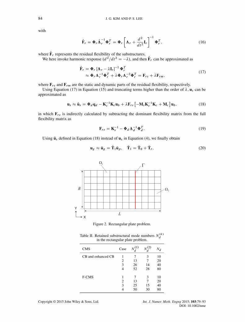
Figure 4. Relative eigenvalue errors in the rectangular plate problem. (c) Nd D 40 and (d) Nd D 80.



QMp D NTT1 MgNT1 D NMp C NTTr Mg

NT0 C NTT0 MgNTr C NTTr Mg

NTr ; (24a)QKp D NTT1 Kg

NT1 D NKp C NTTr KgNT0 C NTT0 Kg

NTr C NTTr KgNTr : (24b)

Because of the compensation of the residual substructural modes in NT1, the reduced mass andstiffness matrices in Equation (24) are more precisely constructed than the original reduced matricesin Equation (8). For this reason, when the newly defined QMp and QKp are used in Equation (9), thesolution accuracy of the reduced eigenvalue problem can be improved.

Table I shows the comparison of the original and enhanced CB methods. It is important to notethat both methods (original and enhanced) produce reduced models of the same size. Comparedwith the original CB method, the residual flexibility Frs and the inverse of the reduced mass matrixNM�1p are additionally computed to construct the enhanced transformation matrix NT1 in the enhanced

CB method.However, Frs can be simply calculated by reusing K�1s in Equation (4) and the dominant sub-

structural eigensolutions in Equation (7) (Equation (19)). Also, the size of the reduced mass matrixNMp is small because it consists of a small number of dominant substructural modes and interface

DOFs. For these reasons, we can easily identify the fact that the additional computational cost ofthe enhanced CB method is not high.

Note that the concept of the residual flexibility OFr in Equation (16) is essential for CMS methodswith free interface boundary [9–11, 19], but the concept has not been employed for the improve-ment of CMS methods with fixed interface boundary (like the CB and Automated Multi-LevelSubstructuring (AMLS) methods) [3, 8].

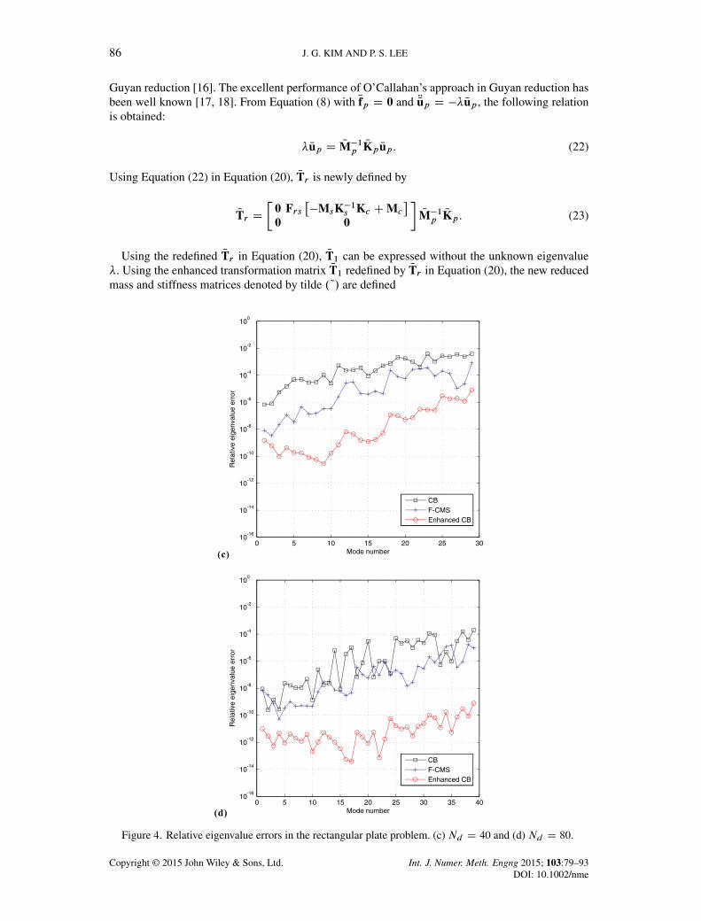
Figure 5. Hyperboloid shell problem.



4. NUMERICAL EXAMPLES

In this section, we test the performance of the enhanced CB method compared with the original CBand F-CMS methods. It should be noted that, because of the use of localized Lagrange multipliers[9, 19], the F-CMS method generally requires more DOFs in reduced models (larger size of reducedmatrices) than the original and enhanced CB methods for the same number of retained dominantsubstructural modes.

Four different structural problems are considered: rectangular plate, hyperboloid shell, stiffenedplate, and solid ring problems. These are modeled by four-node Mixed Interpolation of TensorialComponents (MITC) shell (e.g., [20–23]) and eight-node brick elements. We here use the frequencycutoff mode selection method [24] to select the dominant substructural modes.

Table III. Retained substructural mode numbers N .k/d

in the hyper-boloid shell problem.

CMS Case N.1/d

N.2/d

N.3/d

N.4/d

Nd

CB and enhanced CB 1 17 3 17 3 402 33 7 33 7 80

F-CMS 1 15 5 15 5 402 29 11 29 11 80

Figure 6. Relative eigenvalue errors in the hyperboloid shell problem. (a) Nd D 40 and (b) Nd D 80.



The following relative eigenvalue error is used to evaluate the performance of the enhancedCB method:

�i DN�i � �i

�i; (25)

in which �i denotes the relative eigenvalue error for the i-th mode, and �i and N�i are the exact andapproximated eigenvalues, respectively. These eigenvalues are calculated from the global (original)and reduced eigenvalue problems (Equations (2) and (9)).

4.1. Rectangular plate problem

Let us consider a rectangular plate with free boundary as shown in Figure 2. Length L is 0.6096 m,width B is 0.3048 m, and thickness h is 3:175 � 10�3 m. Young’s modulus E is 72G Pa, Poisson’sratio � is 0.33, and density �s is 2796 kg/m3. The plate is modeled by a 12�6mesh of the four-nodeMITC shell FEs, and the structural model is partitioned into two substructures .Ns D 2/.

We consider four numerical cases with 10, 20, 40, and 80 dominant substructural modes selected.The numbers of retained substructural modes N .k/

dare listed in Table II. Figures 3 and 4 present

the relative eigenvalue errors obtained by the original CB, F-CMS, and enhanced CB methods. Theresults show that the enhanced CB method outperforms the other two methods regardless of thenumber of retained substructural modes.

Figure 7. Stiffened plate problem.



Table IV. Retained substructural mode numbers N .k/d

in the stiffened plate problem.

CMS Case N.1/d

N.2/d

N.3/d

N.4/d

N.5/d

N.6/d

Nd

CB and enhanced CB 1 20 8 3 3 8 8 502 29 17 6 6 11 11 80

F-CMS 1 11 11 7 7 7 7 502 18 18 11 11 11 11 80

Figure 8. Relative eigenvalue errors in the stiffened plate problem. (a) Nd D 50 and (b) Nd D 80.

4.2. Hyperboloid shell problem

We here consider a hyperboloid shell structure of height H D 4:0 m and thickness h D 0:05 m.Young’s modulus E is 69 GPa, Poisson’s ratio � is 0.35, and density �s is 2700 kg/m3. The mid-surface of this shell structure is described by

x2 C y2 D 2C ´2I ´ 2 Œ�2; 2�: (26)

We use a mesh of 20 (axial) � 40 (circumferential) MITC4 shell elements (Figure 5). The FEmodel of the hyperboloid shell is partitioned into four substructures .Ns D 4/.



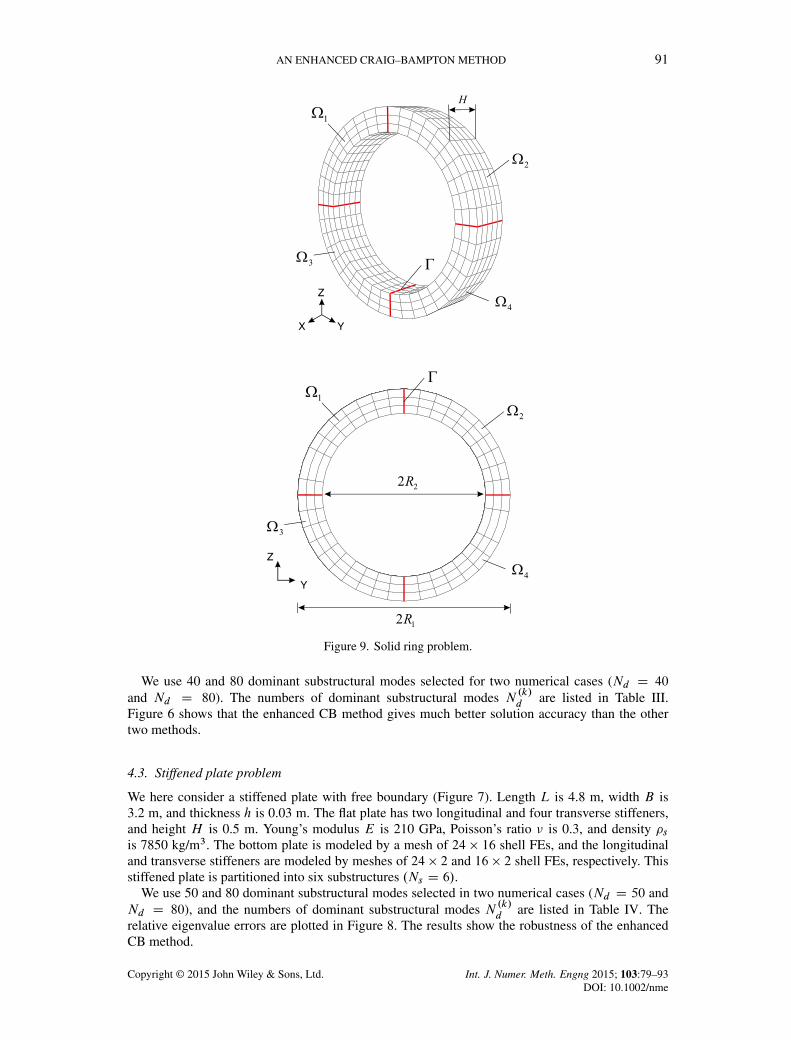
Figure 9. Solid ring problem.

We use 40 and 80 dominant substructural modes selected for two numerical cases (Nd D 40

and Nd D 80). The numbers of dominant substructural modes N .k/

dare listed in Table III.

Figure 6 shows that the enhanced CB method gives much better solution accuracy than the othertwo methods.

4.3. Stiffened plate problem

We here consider a stiffened plate with free boundary (Figure 7). Length L is 4.8 m, width B is3.2 m, and thickness h is 0.03 m. The flat plate has two longitudinal and four transverse stiffeners,and height H is 0.5 m. Young’s modulus E is 210 GPa, Poisson’s ratio � is 0.3, and density �sis 7850 kg/m3. The bottom plate is modeled by a mesh of 24 � 16 shell FEs, and the longitudinaland transverse stiffeners are modeled by meshes of 24 � 2 and 16 � 2 shell FEs, respectively. Thisstiffened plate is partitioned into six substructures .Ns D 6/.

We use 50 and 80 dominant substructural modes selected in two numerical cases (Nd D 50 andNd D 80), and the numbers of dominant substructural modes N .k/

dare listed in Table IV. The

relative eigenvalue errors are plotted in Figure 8. The results show the robustness of the enhancedCB method.



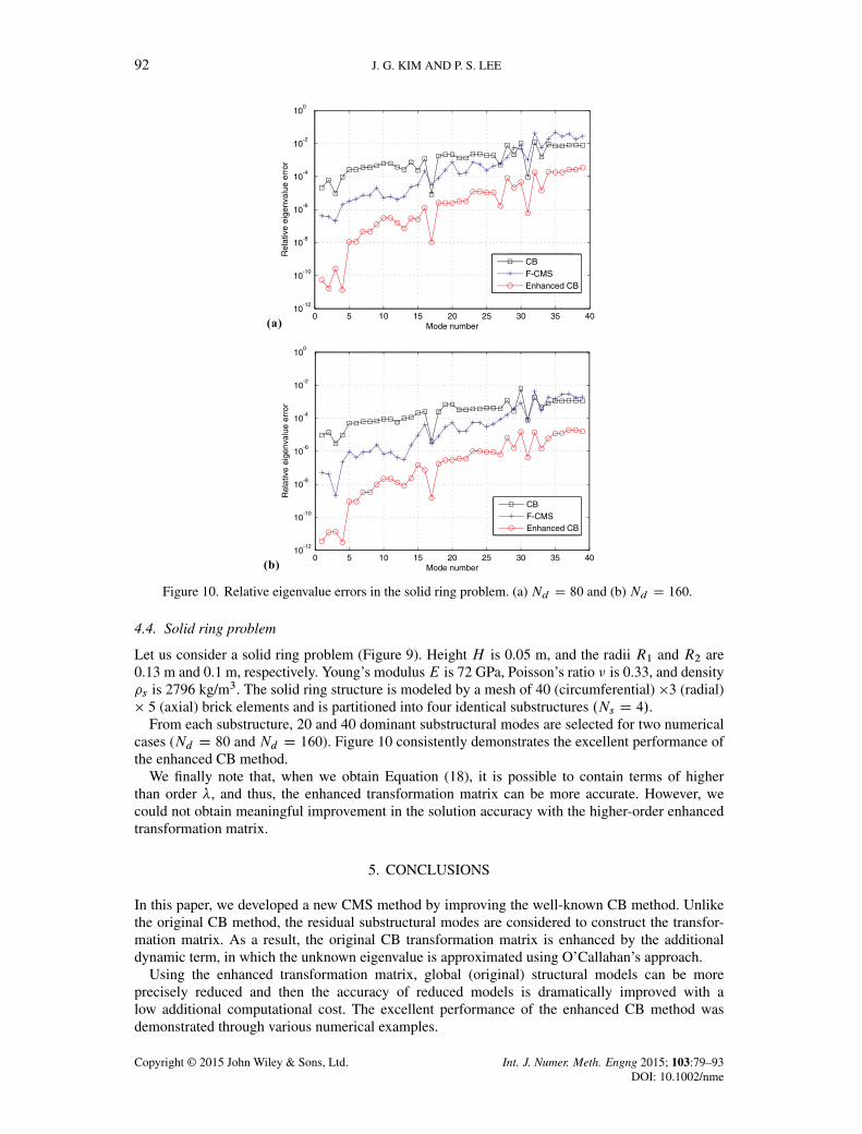
Figure 10. Relative eigenvalue errors in the solid ring problem. (a) Nd D 80 and (b) Nd D 160.

4.4. Solid ring problem

Let us consider a solid ring problem (Figure 9). Height H is 0.05 m, and the radii R1 and R2 are0.13 m and 0.1 m, respectively. Young’s modulus E is 72 GPa, Poisson’s ratio � is 0.33, and density�s is 2796 kg/m3. The solid ring structure is modeled by a mesh of 40 (circumferential) �3 (radial)� 5 (axial) brick elements and is partitioned into four identical substructures .Ns D 4/.

From each substructure, 20 and 40 dominant substructural modes are selected for two numericalcases (Nd D 80 and Nd D 160). Figure 10 consistently demonstrates the excellent performance ofthe enhanced CB method.

We finally note that, when we obtain Equation (18), it is possible to contain terms of higherthan order �, and thus, the enhanced transformation matrix can be more accurate. However, wecould not obtain meaningful improvement in the solution accuracy with the higher-order enhancedtransformation matrix.

5. CONCLUSIONS

In this paper, we developed a new CMS method by improving the well-known CB method. Unlikethe original CB method, the residual substructural modes are considered to construct the transfor-mation matrix. As a result, the original CB transformation matrix is enhanced by the additionaldynamic term, in which the unknown eigenvalue is approximated using O’Callahan’s approach.

Using the enhanced transformation matrix, global (original) structural models can be moreprecisely reduced and then the accuracy of reduced models is dramatically improved with alow additional computational cost. The excellent performance of the enhanced CB method wasdemonstrated through various numerical examples.



To practically use the enhanced CB method, mode selection and error estimation techniques areessential [15, 19, 25], and also, the conceptual idea of the enhanced CB method would be used toimprove other CMS methods.

ACKNOWLEDGEMENTS

This work was supported by the Basic Science Research Program through the National ResearchFoundation of Korea (NRF) funded by the Ministry of Education, Science and Technology(No.2014R1A1A1A05007219), and the grant NEMA-NH-2012-69 from the Natural Hazard MitigationResearch Group, National Emergency Management Agency of Korea.

REFERENCES

1. Hurty W. Dynamic analysis of structural systems using component modes. AIAA Journal 1965; 3(4):678–685.2. Guyan R. Reduction of stiffness and mass matrices. AIAA Journal 1965; 3(2):380.3. Craig RR, Bampton MCC. Coupling of substructures for dynamic analysis. AIAA Journal 1968; 6(7):1313–1319.4. MacNeal RH. Hybrid method of component mode synthesis. Computers & Structures 1971; 1(4):581–601.5. Benfield WA, Hruda RF. Vibration analysis of structures by component mode substitution. AIAA Journal 1971;

9:1255–1261.6. Rubin S. Improved component-mode representation for structural dynamic analysis. AIAA Journal 1975; 13(8):

995–1006.7. Hintz RM. Analytical methods in component modal synthesis. AIAA Journal 1975; 13(8):1007–1016.8. Bennighof JK, Lehoucq RB. An automated multilevel substructuring method for eigenspace computation in linear

elastodynamics. SIAM Journal on Scientific Computing 2004; 25(6):2084–2106.9. Park KC, Park YH. Partitioned component mode synthesis via a flexibility approach. AIAA Journal 2004;

42(6):1236–1245.10. Rixen DJ. A dual Craig-Bampton method for dynamic substructuring. Journal of Computational and Applied

Mathematics 2004; 168(1-2):383–391.11. Markovic D, Park KC, Ibrahimbegovic A. Reduction of substructural interface degrees of freedom in flexibility-based

component mode synthesis. International Journal of Numerical Methods in Engineering 2007; 70:163–180.12. Craig RR. Coupling of substructures for dynamic analyses: an overview. in: Proceeding 41th

AIAA/ASME/ASCE/AHS/ASC Structures, Structural Dynamics, and Materials Conference, Atlanta, USA, 2000;AIAA 2000–1573.

13. Craig RR, Kurdila AJ. Fundamentals of Structural Dynamics. Wiley: New York, 2006.14. Klerk DD, Rixen DJ, Voormeeren SN. General framework for dynamic substructuring: history, review, and

classification of techniques. AIAA Journal 2008; 46(5):1169–1181.15. Kim JG, Lee KH, Lee PS. Estimating relative eigenvalue errors in the Craig-Bampton method. Computers &

Structures 2014; 139:54–64.16. O’Callahan J. A procedure for an improved reduced system (IRS) model. Proceeding the 7th International Modal

Analysis Conference, CT, Bethel, 1989; 17–21.17. Friswll MI, Garvey SD, Penny JET. Model reduction using dynamic and iterated IRS techniques. Journal of Sound

and Vibration 1995; 186:311–323.18. Xia Y, Lin R. A new iterative order reduction (IOR) method for eigensolutions of large structures. International

Journal for Numerical Methods in Engineering 2004; 59(1):153–172.19. Park KC, Kim JG, Lee PS. A mode selection criterion based on flexibility approach in component mode synthesis.

Proceeding 53th AIAA/ASME/ASCE/AHS/ASC Structures, Structural Dynamics, and Materials Conference, Hawaii,USA, 2012; AIAA 2012–1883.

20. Dvorkin EN, Bathe KJ. A continuum mechanics based four-node shell element for general nonlinear analysis.Engineering Computations 1984; 1(1):77–88.

21. Bathe KJ, Dvorkin EN. A formulation of general shell elements-the use of mixed interpolation of tensorialcomponents. International Journal for Numerical Methods in Engineering 1986; 22(3):697–722.

22. Lee Y, Lee PS, Bathe KJ. The MITC3+ shell finite element and its performance. Computers & Structures 2014;138:12–23.

23. Jeon HM, Lee PS, Bathe KJ. The MITC3 shell finite element enriched by interpolation covers. Computers &Structures 2014; 134:128–142.

24. Hurty W. A criterion for selecting realistic natural modes of a structure. Technical Memorandum, Jet PropulsionLaboratory, Pasadena, CA, 1967; 33–364.

25. Kim JG, Lee PS. An accurate error estimator for Guyan reduction. Computer Methods in Applied Mechanics andEngineering 2014; 279:1–19.


an enhanced craig–bampton method - cmss laboratorycmss.kaist.ac.kr/cmss/papers/2015 an enhanced...

Documents