an evaluation of structural loop analysis on …...university of southampton an evaluation of...
TRANSCRIPT

UNIVERSITY OF SOUTHAMPTON
An Evaluation of Structural Loop
Analysis on Dynamic Models of
Ecological and Socio-Ecological Systems
by
Joseph J. Abram
A thesis submitted in partial fulfillment for the
degree of Doctor of Philosophy
in the
Faculty of Social, Human and Mathematical Sciences
Geography and Environment
October 2018


UNIVERSITY OF SOUTHAMPTON
ABSTRACT
FACULTY OF SOCIAL, HUMAN AND MATHEMATICAL SCIENCES
GEOGRAPHY AND ENVIRONMENT
Doctor of Philosophy
by Joseph J. Abram

iv
Abstract
This thesis evaluates a modelling analysis technique known as Loop Eigenvalue Elas-
ticity Analysis for its utility and application to system dynamic models of ecological
and socio-ecological systems. The technique acts as a structural analysis of the inter-
actions within the system and is capable of identifying feedback loops as structural
drivers of dynamic behaviour. With adverse behaviours of many ecological systems
known to be driven by feedback mechanisms, Structural Loop Analysis could become
an important method for increasing our understanding and control over the systems
on which we so greatly depend. Within this thesis, a detailed account of the method-
ology and application of structural loop analysis to ecological dynamic models is un-
dertaken. The focus of the thesis is an assessment of the technique for its ability to
improve model design, to increase understanding of system behaviour and ultimately
to evaluate if it could be used for the design and implementation of policy surrounding
complex ecological and socio-ecological systems.
Dynamic system models are predominantly used for exploring the interactions which
occur within and between systems. Dynamic system models are used across a wealth
of academic fields and, much like the purpose of other models, allow the user to ex-
plore and manipulate a system where tests on its real-world equivalent would be im-
practical or unethical to carry out. Through the exploration of components interac-
tions it is possible to learn about, observe and simulate endogenous drivers of systems
as causes of dynamic behaviour and change. While the development and simulation
of a dynamic system model can provide a wealth of information over a target system,
model output alone can often generate more questions than were initially being asked.
Converting a real world system to model format can often lead to black box models,
where the combination of multiple system components and interactions between them
generate unexpected dynamics, even when interactions at a local level are well under-
stood. The complexity that is inherent to our worldly systems can often translate into
the models used to represent them.
Within the fields of ecology and socio-ecology, the occurrence of black box models is
common and seldom a surprise to the multi-disciplinary approach to system under-
standing. Ecological and socio-ecological systems are highly complex, naturally incor-
porating social aspects of human activity and decision making with the natural world,
generating an array of human-environment interactions and forming multiple feedback
mechanisms between the two spheres. Models of these systems can quickly become
just as difficult to interpret as the real world systems, limiting our ability to run and
understand sensitivity analysis, conduct meaningful scenario testing or use these mod-
els to reflect on policy implementation. Maintaining ecological systems in desirable
states is key to developing a growing economy, alleviating poverty and achieving a sus-
tainable future. While the driving forces of an environmental system are often well

v
known, the dynamics impacting these drivers can be hidden within a complex struc-
ture of causal chains and feedback loops.
It is important that we are always on the lookout for new modelling methods, devel-
oping and learning new ways to represent the dynamics and behaviours capable by our
target system. Modelling analysis tools are an important step in the modelling pro-
cess, able to extract additional information of a target system that is often unavailable
from model output alone. Exploring analysis tools can bring new techniques and new
understanding to our model systems which translates to a greater knowledge and un-
derstanding of the target system.
This work was supported by an EPSRC Doctoral Training Centre grant (EP/G03690X/1)

vi

Contents
1 Introduction 1
1.1 Research Questions and Motivations . . . . . . . . . . . . . . . . . . . . . 3
1.2 The Immediate Audience . . . . . . . . . . . . . . . . . . . . . . . . . . . 3
1.3 Outline of Thesis . . . . . . . . . . . . . . . . . . . . . . . . . . . . . . . . 5
1.4 Concepts and Considerations . . . . . . . . . . . . . . . . . . . . . . . . . 8
1.4.1 In Need of a Second Planet . . . . . . . . . . . . . . . . . . . . . . 8
1.4.2 All models are wrong, but some are useful . . . . . . . . . . . . . . . 10
1.4.3 Current System Dynamic Models in Ecology and Socio-Ecology . . 11
1.4.4 The Ambiguity of Model output . . . . . . . . . . . . . . . . . . . 12
1.4.5 Working towards a solution: A Metamodeling approach . . . . . . 13
1.4.6 Loop Eigenvalue Elasticity Analysis (LEEA): A Structural Anal-ysis Technique to be Tested on Ecological models . . . . . . . . . . 13
1.4.7 Socio-Ecology vs Social-Ecology: a note from the author . . . . . . 15
2 Literature Review 17
2.1 System Dynamics: A Modelling Tool Appropriate For Dynamic SystemsModelling . . . . . . . . . . . . . . . . . . . . . . . . . . . . . . . . . . . . 17
2.1.1 What is System Dynamics? . . . . . . . . . . . . . . . . . . . . . . 17
2.1.2 The Origin and Development of System Dynamics . . . . . . . . . 20
2.1.3 Construction of a System Dynamic Model . . . . . . . . . . . . . . 21
2.1.4 Issues associated with system dynamics and alternative methods . 22
2.1.5 Why Study System Structure? . . . . . . . . . . . . . . . . . . . . 24
2.1.6 Complexity within systems . . . . . . . . . . . . . . . . . . . . . . 25
2.1.7 Delays in feedback systems . . . . . . . . . . . . . . . . . . . . . . 26
2.1.8 System Dynamics and Policy . . . . . . . . . . . . . . . . . . . . . 26
2.1.9 The role of System Dynamics to Ecological and Socio-EcologicalSystems . . . . . . . . . . . . . . . . . . . . . . . . . . . . . . . . . 27
2.1.10 The role of Feedback Loops in System Dynamics . . . . . . . . . . 29
2.2 Ecological and Socio-Ecological Systems: An Overview . . . . . . . . . . . 30
2.2.1 Why Study Ecological and Socio-Ecological Systems? . . . . . . . 31
2.2.2 Dynamic Behaviors of Ecosystems . . . . . . . . . . . . . . . . . . 32
2.2.3 Current practices for investigating ecological and socio-ecologicalsystems . . . . . . . . . . . . . . . . . . . . . . . . . . . . . . . . . 36
2.2.4 Modelling of Ecological systems . . . . . . . . . . . . . . . . . . . . 37
2.3 Analytical Techniques . . . . . . . . . . . . . . . . . . . . . . . . . . . . . 39
2.3.1 Traditional Control Theory . . . . . . . . . . . . . . . . . . . . . . 40
2.3.2 Causal Loop Diagrams and System Archetypes . . . . . . . . . . . 41
vii

viii CONTENTS
2.3.3 Ford’s Behavioural Approach . . . . . . . . . . . . . . . . . . . . . 42
2.3.4 Pathway Participation Metrics (PPM) . . . . . . . . . . . . . . . . 42
2.3.5 Eigenvalue Elasticity Analysis (EEA) . . . . . . . . . . . . . . . . 43
2.3.6 Loop Eigenvalue Elasticity Analysis (LEEA) . . . . . . . . . . . . 44
2.3.7 Eigenvector Approach (EVA) & Dynamic Decomposition WeightsAnalysis (DDWA) . . . . . . . . . . . . . . . . . . . . . . . . . . . 44
2.3.8 An Analysis Best Suited for Structural Analysis of Dynamic Sys-tems . . . . . . . . . . . . . . . . . . . . . . . . . . . . . . . . . . . 50
2.3.9 Comments & Reflections . . . . . . . . . . . . . . . . . . . . . . . . 50
2.3.10 Personal communications with Prof. C. E. Kampmann (2015) . . . 51
2.4 Model and Analysis Validation . . . . . . . . . . . . . . . . . . . . . . . . 54
2.4.1 Validation of LEEA and its outputs . . . . . . . . . . . . . . . . . 55
3 Methodology 57
3.1 Loop Eigenvalue Elasticity Analysis (LEEA) . . . . . . . . . . . . . . . . 57
3.1.1 Constructing Differential Equations . . . . . . . . . . . . . . . . . 59
3.1.2 The Jacobian Matrix . . . . . . . . . . . . . . . . . . . . . . . . . . 60
3.1.3 Calculating Eigenvalues . . . . . . . . . . . . . . . . . . . . . . . . 61
3.1.4 Identifying the feedback loops in the Shortest Independent LoopSet (SILS) . . . . . . . . . . . . . . . . . . . . . . . . . . . . . . . . 66
3.1.5 Loop Gains . . . . . . . . . . . . . . . . . . . . . . . . . . . . . . . 67
3.1.6 Loop Eigenvalue Elasticity . . . . . . . . . . . . . . . . . . . . . . 67
3.1.7 Loop Influence . . . . . . . . . . . . . . . . . . . . . . . . . . . . . 69
3.2 A Worked Example: Forming the Jacobian Matrix and its connectionsto Feedback Loops . . . . . . . . . . . . . . . . . . . . . . . . . . . . . . . 71
3.3 Interpretation of Outputs . . . . . . . . . . . . . . . . . . . . . . . . . . . 73
3.4 Regarding Error in LEEA . . . . . . . . . . . . . . . . . . . . . . . . . . . 78
3.5 When to use and when not to use LEEA . . . . . . . . . . . . . . . . . . . 79
3.6 Regarding LEEA’s ability to analyse system’s structure inside vs. out-side a loop. . . . . . . . . . . . . . . . . . . . . . . . . . . . . . . . . . . . 80
4 Structural Loop Analysis of Complex Ecological Systems 83
4.1 Abstract . . . . . . . . . . . . . . . . . . . . . . . . . . . . . . . . . . . . . 83
4.2 Introduction . . . . . . . . . . . . . . . . . . . . . . . . . . . . . . . . . . . 84
4.3 Background . . . . . . . . . . . . . . . . . . . . . . . . . . . . . . . . . . . 86
4.4 Methodology . . . . . . . . . . . . . . . . . . . . . . . . . . . . . . . . . . 88
4.5 Results . . . . . . . . . . . . . . . . . . . . . . . . . . . . . . . . . . . . . . 90
4.6 Discussion . . . . . . . . . . . . . . . . . . . . . . . . . . . . . . . . . . . . 101
4.7 Conclusion . . . . . . . . . . . . . . . . . . . . . . . . . . . . . . . . . . . 105
5 PLUM Model Extensions 109
5.1 Abstract . . . . . . . . . . . . . . . . . . . . . . . . . . . . . . . . . . . . . 109
5.2 Introduction . . . . . . . . . . . . . . . . . . . . . . . . . . . . . . . . . . . 111
5.3 Background . . . . . . . . . . . . . . . . . . . . . . . . . . . . . . . . . . . 112
5.4 Methodology . . . . . . . . . . . . . . . . . . . . . . . . . . . . . . . . . . 114
5.5 PLUMGov Model . . . . . . . . . . . . . . . . . . . . . . . . . . . . . . . . 115
5.6 PLUMGov Results . . . . . . . . . . . . . . . . . . . . . . . . . . . . . . . 117
5.7 PLUMPlus Model . . . . . . . . . . . . . . . . . . . . . . . . . . . . . . . 122

CONTENTS ix
5.8 PLUMPlus Results . . . . . . . . . . . . . . . . . . . . . . . . . . . . . . . 126
5.9 Yulin City Model . . . . . . . . . . . . . . . . . . . . . . . . . . . . . . . . 131
5.10 Discussion . . . . . . . . . . . . . . . . . . . . . . . . . . . . . . . . . . . . 133
5.11 Concluding Statements . . . . . . . . . . . . . . . . . . . . . . . . . . . . . 136
6 Accessing LEEA’s Niche: An Analysis Comparison in the Context of Lever-age Points 139
6.1 Abstract . . . . . . . . . . . . . . . . . . . . . . . . . . . . . . . . . . . . . 139
6.2 Introduction . . . . . . . . . . . . . . . . . . . . . . . . . . . . . . . . . . . 141
6.3 Background . . . . . . . . . . . . . . . . . . . . . . . . . . . . . . . . . . . 142
6.4 Methodology . . . . . . . . . . . . . . . . . . . . . . . . . . . . . . . . . . 146
6.5 Results . . . . . . . . . . . . . . . . . . . . . . . . . . . . . . . . . . . . . . 151
6.6 Discussion . . . . . . . . . . . . . . . . . . . . . . . . . . . . . . . . . . . . 163
6.7 Conclusion . . . . . . . . . . . . . . . . . . . . . . . . . . . . . . . . . . . 167
7 LEEA’s Application to a Coral Reef System Capable of Alternative States- Multiple Feedback Analysis 169
7.1 Abstract . . . . . . . . . . . . . . . . . . . . . . . . . . . . . . . . . . . . . 169
7.2 Introduction . . . . . . . . . . . . . . . . . . . . . . . . . . . . . . . . . . . 171
7.3 Background . . . . . . . . . . . . . . . . . . . . . . . . . . . . . . . . . . . 173
7.4 Methodology . . . . . . . . . . . . . . . . . . . . . . . . . . . . . . . . . . 177
7.5 Results . . . . . . . . . . . . . . . . . . . . . . . . . . . . . . . . . . . . . . 184
7.6 Discussion . . . . . . . . . . . . . . . . . . . . . . . . . . . . . . . . . . . . 187
7.7 Conclusion . . . . . . . . . . . . . . . . . . . . . . . . . . . . . . . . . . . 190
8 Discussion 191
8.1 A summary of the studies within this thesis . . . . . . . . . . . . . . . . . 192
8.1.1 Chapter 4: The PLUM model . . . . . . . . . . . . . . . . . . . . . 192
8.1.2 Chapter 5: Investigating LEEA’s limitations . . . . . . . . . . . . 192
8.1.3 Chapter 6: LEEA, DDWA and Sensitivity Analysis . . . . . . . . . 192
8.1.4 Chapter 7: Coral reef model . . . . . . . . . . . . . . . . . . . . . . 193
8.2 A review of the research questions and motivations of the thesis . . . . . . 193
8.3 The Implementation of LEEA as a Standard Analytical Tool . . . . . . . 197
8.3.1 Where LEEA sits among current techniques . . . . . . . . . . . . . 197
8.3.2 Implementing LEEA into Standard practices . . . . . . . . . . . . 197
8.3.3 Model Design and Construction: Participatory Complexity Science 201
8.3.4 LEEA and model adaptability . . . . . . . . . . . . . . . . . . . . 203
8.3.5 Using LEEA for System Maintenance . . . . . . . . . . . . . . . . 204
8.4 Levarage points, Policy and LEEA . . . . . . . . . . . . . . . . . . . . . . 205
8.4.1 A review of ecological modelling and policy . . . . . . . . . . . . . 205
8.4.2 Identifying System Leverage Points . . . . . . . . . . . . . . . . . . 208
8.4.3 The application of LEEA to policy design and implementation . . 209
8.4.4 Acknowledging LEEA’s limitations in the context of ecologicalmodelling and policy making . . . . . . . . . . . . . . . . . . . . . 210
8.5 Exploring LEEA’s limitations . . . . . . . . . . . . . . . . . . . . . . . . . 211
8.6 LEEA in Qualitative Modelling . . . . . . . . . . . . . . . . . . . . . . . . 213
8.6.1 Early Model Design and consequences to LEEA: A Case Study . . 213

x CONTENTS
8.6.2 Is There A Place For Qualitative Modelling Within System Dy-namics? . . . . . . . . . . . . . . . . . . . . . . . . . . . . . . . . . 218
8.7 The future for LEEA - Steering Complex Systems . . . . . . . . . . . . . 221
8.8 Future Work - What Next? . . . . . . . . . . . . . . . . . . . . . . . . . . 222
8.9 Importance of Accessibility: A Review of LEEA Implementation andSubject Terminology . . . . . . . . . . . . . . . . . . . . . . . . . . . . . . 223
8.9.1 Improving LEEA Accessibility . . . . . . . . . . . . . . . . . . . . 223
8.9.2 Accessibility of system dynamic modelling to the public and pol-icy makers . . . . . . . . . . . . . . . . . . . . . . . . . . . . . . . . 225
8.9.3 Discussion on the terms positive and negative feedback: . . . . . . 225
9 Conclusions 229
9.1 Supplementary Information 2: LEEA Processing Details . . . . . . . . . . 236
Bibliography 237

List of Figures
2.1 An example of a system dynamic model using a classic Lokta-Volterrasystem. The diagram shows examples of stocks, flows, auxiliary vari-ables, sources, sinks, and links which carry information between systemcomponents. . . . . . . . . . . . . . . . . . . . . . . . . . . . . . . . . . . . 19
2.2 Extracted from Wolstenholme (2003) displaying the basic form of a sys-tem archetype. . . . . . . . . . . . . . . . . . . . . . . . . . . . . . . . . . 41
2.3 Extracted from Kampmann and Oliva (2008) showing a visual repre-sentation of procedures and order of operations to carry out LEEA andDDWA . . . . . . . . . . . . . . . . . . . . . . . . . . . . . . . . . . . . . . 45
3.1 A visual respresentation of a stock variable (black box), its flows (dou-ble lined black arrows), sources and sinks (cloud shapes). The image isextracted from a Vensim model and translates to the following dynami-cal equation: δIS
δt = newindustries− demolition . . . . . . . . . . . . . . 59
3.2 An eigenvalue plot produced from LEEA of a seven stock system. Eachline represents a different eigenvalue of the system as it changes throughthe simulation. . . . . . . . . . . . . . . . . . . . . . . . . . . . . . . . . . 64
3.3 An eigenvalue plot of a seven stock system sectioned into managableparts fo analysis. . . . . . . . . . . . . . . . . . . . . . . . . . . . . . . . . 64
3.4 The system dynamic form of the predador- prey equations. This dia-gram is an example of how one might find an system dynamic model,with variables labelled as opposed to their equation equivalents. . . . . . 71
3.5 The system dynamic form of the predador- prey equations. This dia-gram shows how all of the equations of Lokta-Volterra fit into systemdynamic model form. . . . . . . . . . . . . . . . . . . . . . . . . . . . . . . 72
3.6 Data series from an eigenvalue calculation (real part) showing 21 timesteps from 60-80. Columns 2-4 represent eigenvalues 1 2 and 3 of thesystem. . . . . . . . . . . . . . . . . . . . . . . . . . . . . . . . . . . . . . 74
3.7 Data series from an eigenvalue calculation (imaginary part) showing 21time steps from 60-80. Columns 2-4 represent eigenvalues 1 2 and 3 ofthe system. . . . . . . . . . . . . . . . . . . . . . . . . . . . . . . . . . . . 74
3.8 Real and Imaginary eigenvalues presented in graphical form. The x axisis the real part and y axis the imaginary part. Eigenvalues are repre-sented with blue dots. This graphical form shows just one time step inthe data series. . . . . . . . . . . . . . . . . . . . . . . . . . . . . . . . . . 74
3.9 Real Eigenvalues plotted through time, each line represents the changein one eigenvalue and the red box highlights timesteps 60 to 80. . . . . . . 75
xi

xii LIST OF FIGURES
3.10 Real and Imaginary results of feedback Loop influence plotted throughtime in graphical form, where each line represents a separate feedbackstructure of the system. . . . . . . . . . . . . . . . . . . . . . . . . . . . . 76
3.11 Feedback loop influence showing subsection of the real part with a spec-ified shorter range for closer interpretation of results. . . . . . . . . . . . . 77
3.12 Feedback loop influence showing absolute values. . . . . . . . . . . . . . . 77
3.13 A) Feedback loop influence values of seven loop structures for a singlepoint in time of a simulation. The values are displayed as absolute val-ues and their real part. B) Feedback loop influence values plotted ingraphical form . . . . . . . . . . . . . . . . . . . . . . . . . . . . . . . . . 78
3.14 Example of a chain and loop structure connected to form part of alarger model structure. Letters a to f represent non specified auxillaryvariables within a causal chain leading into the feedback structure. . . . . 81
4.1 a. The PLUM model a structural representation of Carpenter’s phos-phorus equations (Carpenter 2005) containing the stocks (black boxes)water phosphorus density (P), soil phosphorus density (U) and sedi-ment phosphorus density (M). The figure also contains system flows(black double arrows) going into and out of each stock, sources andsinks (cloud shapes) and component interactions (blue arrows). . Therecreation of Scenario 1 can be seen in figure b. The extension to theCarpenter simulation, to invoke a reverse critical transition in the sys-tem can be seen in c. . . . . . . . . . . . . . . . . . . . . . . . . . . . . . . 94
4.2 a) Shows the forward critical transition from years 250-999 from Sce-nario 1 of Carpenter (2005). b) Loop Gain values for the forward criti-cal transition between years 435-460. c) The system’s three eigenvaluescalculated and plotted through time for the forward critical transition.The red box shows a zoom of the eigenvalues changing to positive po-larity. d) Loop influence values within Eigenvalue 1 for years 435-460.Plots b,c and d are generated from Naumov & Oliva (2017) online ma-terial. . . . . . . . . . . . . . . . . . . . . . . . . . . . . . . . . . . . . . . 96
4.3 a) Shows the reverse critical transition from years 1000-2500 from theextension to Scenario 1 of Carpenter (2005). b) Loop Gain values forthe reverse critical transition between years 2040 and 2065. c) The sys-tem’s three eigenvalues calculated and plotted through time for the re-verse critical transition. d) Loop influence values within Eigenvalue 1for years 2040 to 2065. e) Loop influence values within Eigenvalue 2 foryears 2040 to 2065. Plots b, c, d and e are generated from Naumov &Oliva (2017) online material. . . . . . . . . . . . . . . . . . . . . . . . . . 99
4.4 A) Shows Loop 5, the positive feedback loop shown from LEEA to gen-erate instability within the system leading up to the critical transitions.B) Shows Loop 2, a negative feedback loop responsible for most of thestability within the system. . . . . . . . . . . . . . . . . . . . . . . . . . . 101
5.1 The PLUMGov Model. An extension of the PLUM model by inclusionof Government intervention which activates when the phosphorus levelsget too high. . . . . . . . . . . . . . . . . . . . . . . . . . . . . . . . . . . 116
5.2 Water phosphorus output of the PLUMGov model showing forward andreverse critical transitions across a 1000 year time period. . . . . . . . . . 117

LIST OF FIGURES xiii
5.3 Eigenvalues from PLUMGov. 2a shows real values.2b shows imaginaryvalues. . . . . . . . . . . . . . . . . . . . . . . . . . . . . . . . . . . . . . . 118
5.4 Loop gain values of PLUMGov . . . . . . . . . . . . . . . . . . . . . . . . 119
5.5 PLUMGov eigenvalue 1 loop influence values (real part). Each line onthe plots represents 1 of the 7 loops within the system. . . . . . . . . . . . 119
5.6 Loop Influnece values of eigenvalue 3 in the PLUM model leading up tothe forward critical transition. . . . . . . . . . . . . . . . . . . . . . . . . . 120
5.7 Loop Influnece values of eigenvalue 3 in the PLUMGov model leadingup to the forward critical transition. . . . . . . . . . . . . . . . . . . . . . 120
5.8 The system dynamic model of PLUMPlus. An extension to the PLUMmodel by the addition of a local government influence, a local popula-tion, migration into and out of the area and predator prey interactionsbetween Lake Biota and Blue Green Algae. . . . . . . . . . . . . . . . . . 124
5.9 PLUMPlus Stock Outputs. . . . . . . . . . . . . . . . . . . . . . . . . . . 125
5.10 Seven behavioural modes from PLUMPlus. a shows real values, b showsimaginary values. . . . . . . . . . . . . . . . . . . . . . . . . . . . . . . . . 127
5.11 Loop gains of PLUMPlus including 17 loop total. . . . . . . . . . . . . . . 129
5.12 LEEA output for the PLUMPLus model, showing Loop influence out-put from eigenvalue 3. The output includes 17 structural feedback loops,each of which is represented by a single line within the plot. The plot isone of fourteen which would have to be compared in order to determinethe dominant loop structures of the system. . . . . . . . . . . . . . . . . . 129
5.13 Showing how the results of Loop Elasticity can differ so much acrosseigenvalues. . . . . . . . . . . . . . . . . . . . . . . . . . . . . . . . . . . . 130
5.14 Showing the difference between Loop Elasticity Results and Loop Influ-ence results. . . . . . . . . . . . . . . . . . . . . . . . . . . . . . . . . . . . 130
5.15 Structural representation of the Yulin city model adapted from Wanget al. (2011) . . . . . . . . . . . . . . . . . . . . . . . . . . . . . . . . . . . 131
5.16 Loop Gain output from the Yulin City Model giving a first impressionof the dynamics and dominance of the 25 loop structures present withinthe system prior to calculation of loop influence. . . . . . . . . . . . . . . 132
6.1 Eigenvalues weights from DDWA of the PLUM model at t=250 . . . . . . 152
6.2 The PLUM model in system dynamic form . . . . . . . . . . . . . . . . . 153
6.3 An example of how elastcity values from DDWA reflect back on modeloutput, represented using variables m and r. Variable m has a highelasticity value which is negative so a 10% change can makes large dif-ferences to the output, while variable r has a low elasticity, which ispositive so a 10% change makes a relatively small difference to modeloutput. . . . . . . . . . . . . . . . . . . . . . . . . . . . . . . . . . . . . . 155
6.4 Sensitivity outputs for variables W,F,H, c and q. Black line plots onthe left hand side show each of the 200 runs and coloured plots on theright hand side show the range of values within the 50, 75, 95 and 100percentiles. . . . . . . . . . . . . . . . . . . . . . . . . . . . . . . . . . . . 157
6.5 Sensitivity outputs for variables r,m, h, s and b. Black line plots on theleft hand side show each of the 200 runs and coloured plots on the righthand side show the range of values within the 50, 75, 95 and 100 per-centiles. . . . . . . . . . . . . . . . . . . . . . . . . . . . . . . . . . . . . . 158

xiv LIST OF FIGURES
7.1 A replication of ‘All feedbacks’ scenario from Van de Leemput et al.(2016). The red line represents cover by coral. The green line representscover by macroalgae. The blue line represents abundance of herbivores.The bistable zone occurs between 33% and 51% fishing. . . . . . . . . . . 182
7.2 Cyclic diagram of Van de Leemput et al. (2016) scenario ‘All feedbacks’containing all eight loops from the base scenario, labelled 1-8 and thethree extensions which collectively form two new structural loops 9 &10. Any interactions contained within the base scenario are representedwith blue arrows and any interactions from the extension scenarios arerepresented with red arrows. Loops formed by the implementation ofeach scenario have their arrows adapted in the following manner: Sce-nario ii) Herbivory-escape - dashed arrows, Scenario iii) Competition -dotted arrows, Scenario iv) Coral-Herbivore - bold arrows. Interactionswhich are involved in more than one scenario are represented by thescenario which they first appear in. . . . . . . . . . . . . . . . . . . . . . . 183
8.1 The process of participatory complexity science. Adapted from Dr Alexan-dra Penn, 2017 - guest lecturer at Geography and Environment, Southamp-ton University. Originated from ‘Steering Complex Human Systems’(Penn 2017). . . . . . . . . . . . . . . . . . . . . . . . . . . . . . . . . . . 203
8.2 Cyclic diagram of factors affecting the success of a population of Lox-odes rex . . . . . . . . . . . . . . . . . . . . . . . . . . . . . . . . . . . . . 215
8.3 System dynamics diagram of the system drivers and interactions affect-ing Loxodes rex within its local freshwater environment. . . . . . . . . . . 216
8.4 a) adjacency matrix of the variables within the Loxodes rex system dy-namics model. 4 b) reachability matrix of the variables within the Lox-odes rex system dynamics model. Axis represent the number of vari-ables in the model and nz is the number of connections found withinthe structure.. . . . . . . . . . . . . . . . . . . . . . . . . . . . . . . . . . . 217
8.5 Positive Loop Structures . . . . . . . . . . . . . . . . . . . . . . . . . . . . 226
8.6 Negative Loop Structures . . . . . . . . . . . . . . . . . . . . . . . . . . . 226

List of Tables
2.1 Terms associated with ecosystem dynamics and clarification of theirmeaning when used within the context of structural analysis. . . . . . . . 37
4.1 Modified from Carpenter (2005). Model parameters, nominal values andunits used to implement PLUM. . . . . . . . . . . . . . . . . . . . . . . . 92
4.2 Modified from Carpenter (2005). Changes to phosphorus input levelswithin the PLUM model for the first scenario, 0 to 1000 years. . . . . . . 92
4.3 Loop numbers, structures and loop type within the PLUM model. . . . . 94
6.1 DDWA elasticity values for each variable within the PLUM model ofChapter 4, for the Pwater stock (phosphorous density in lake water) . . . 154
6.2 Outputs of variable sensitivity within the PLUM model calculated rel-ative to each system stock. Values highlighted in red register above asensitivity of 1 and are therefore deemed the most sensitive componentsto the system. . . . . . . . . . . . . . . . . . . . . . . . . . . . . . . . . . . 156
6.3 The critical transition, eigenvalue plot and loop influence output ofeigenvalue 1 from the original PLUM model. . . . . . . . . . . . . . . . . 159
6.4 The model output of the Pwater stock, eigenvalue plot and loop influ-ence output of scenario 1: H increase with critical transition. . . . . . . . 160
6.5 The model output of the Pwater stock, eigenvalue plot and loop influ-ence output of scenario 2: H increase without critical transition. . . . . . 161
6.6 The model output of the Pwater stock, eigenvalue plot and loop influ-ence output of scenario 3: Maximum phosphorus output. . . . . . . . . . . 161
6.7 The model output of the Pwater stock, eigenvalue plot and loop influ-ence output of scenario 4: Purposeful reduction in loop influence. . . . . . 162
7.1 Lists the eight loop structures within Van de Leemput et al. (2016) basescenario coral reef system . . . . . . . . . . . . . . . . . . . . . . . . . . . 178
7.2 Lists the feedback loop structures within Van de Leemput et al. (2016)additional scenarios . . . . . . . . . . . . . . . . . . . . . . . . . . . . . . . 180
7.3 Adapted from Van de Leemput et al. (2016). Expresses the symbols,names and values attributed to construct each of the scenarios . . . . . . 181
xv


LIST OF TABLES xvii
Acknowledgements
A great thanks to my supervisor Dr. James Dyke who has always shown interest in
the subject material and given great advice in every meeting while letting me pursue
my own interests within the field. I always came out of a supervisory meeting feel-
ing more positive than when I went in and I cannot thank him enough for his support
during difficult periods. His teaching throughout the years has really helped me to be-
come a better academic and I thank him for truly making my PhD an enjoyable and
unforgettable experience.
Thanks to my co-supervisor Professor John Dearing, whose expert knowledge in the
field provided some great insight into each of my projects and whose suggestions through-
out my time as a PhD student were invaluable. I felt so lucky to have someone with
such an amazing knowledge of the material and thank him for his time, effort and pa-
tience during all of our meetings.
I would like to thank the EPSRC and the Institute for Complex System Simulation
(ICSS) for the funding and opportunity they provided that allowed me to conduct my
PhD. The ability to build my own project with the support and training provided by
the EPSRC and ICSS was the best start to a PhD I could have hoped for. The staff
and fellow PhD students of the Complexity Doctoral Training Centre made my experi-
ence second to none and it was an absolute pleasure to be a part of.
A huge thanks to the Geography and Environment Department who have given amaz-
ing support throughout the years of my PhD and provided a healthy work environ-
ment for me to thrive. I thank them for all of the opportunities to present and im-
prove my work and I wish them all the best with their future PhD students.
My thanks also go to Prof. C. E Kampmann for his advice and help during early stages
of the thesis. His enthusiam for my project and ideas of how to use LEEA gave me a
great deal of confidence while I was planning my thesis and exploring multiple ideas.
To the members of Harbor Branch Oceanographic Institute (HBOI) at Florida Alt-
lantic University, I cannot thank them enough for their hospitatity and the oppor-
tunity that they gave me to not only conduct work abroad but also in an unfamiliar
field, while still feeling like a valuable member of their team. I wish them all the best
for their future endeavours and fully intend to keep in touch throughout my career.
A massive thanks to my family for all of their support. They always made sure that
further education was a top priority and never out of reach, for which I am eternally
grateful. I would like to thank my mum for her endless enthusiasm to read my work
and my dad for his incredible ability to fit an entire flat’s worth of belongings into a
single car each time I moved. I would also like to thank my big sister for being a true

xviii LIST OF TABLES
inspiration to me for the hard work and dedication that she puts into everything she
does.
Finally I would like to thank my friends for keeping me sane throughout my PhD with
a healthy work-life balance and always being there for me when I needed them most.

Chapter 1
Introduction
This work takes interest in human interaction with ecological systems, focusing on the
underlying structural drivers of system behaviour. The work takes a prime interest
in our ability to understand complex system dynamic models. The system dynamic
method has become a popular and resilient modelling technique to capture system
complexity and dynamics (Forrester 2007a; Ford 1999b; Forrester 1994). The system
dynamic method provides a unique perspective regarding system structure and in-
teractions for the discussion of modern society concerns i.e. population growth and
global resource management (Meadows 2008; Meadows et al. 1972).
Ecological and socio-ecological systems (SESs), sometimes referred to as social-environmental
systems, are complex and dynamic whose coupled interactions and exogenous drivers
we may never fully understand. As a society, we are an integrated part of these sys-
tems and are often a keystone species in multiple systems from local to global scale.
Neglect of SESs can lead to a loss of ecosystem services, creating pressure on economic
development and poverty alleviation (Carpenter et al. 2009). Examples include in-
dustrial waste contributing to coral bleaching, reducing tourism and driving away fish
stocks and biodiversity loss driven by deforestation, impacting food security and heav-
ily reducing the monetary value of an ecosystem’s goods and services.
System dynamics, a modelling technique initially developed in the 1950s, has seen a
wide use across ecological systems research. System dynamics is used to simulate po-
tential non-linear behaviour, express multiple interactions and reveal emergent feed-
back structures of complex systems which can prove difficult to understand. In SESs,
it has often been used to understand the interaction between human development and
the environment. System dynamic models may prove to be as intractable as the real
world system they seek to simulate. This work aims to gain insights into the struc-
tural processes and mechanisms underlying the behaviour of the model and the real
world systems they represent. Identifying influential feedback structures of a system
1

2 Chapter 1 Introduction
could have profound implications for the way that we approach model simulation, de-
cision making and policy analysis.
This thesis takes seriously the eight problem areas in system dynamics posed by Richard-
son (1996). Through the exploration of a system dynamic analysis technique, this
work takes direction from three of those problem areas for researchers of ecological
systems: ‘understanding model behaviour’, ‘making models accessible’ and ‘widening
the base’.
‘Understanding model behaviour’: This accounts for how a model’s output is gener-
ated by the system and what system components internally or externally drive its
changes. Through the introduction of structural analysis techniques to a ecological
context, this work investigates bridging the gap between our understanding and abil-
ity to learn from small and large system models. Small system models often contain
drivers which are easy to identify, but contain dynamics and interactions which are
relatively simple representations of real world complexity. On the other hand, large
system models may feature more interactions and dynamics with the assumption that
those elements are necessary to reproduce the behaviour of the system, but the iden-
tification of system drivers gets lost in a giant network of interactions causing the
model’s output to appear as if it had been pulled from a ‘black box’.
‘Making models accessible’: Ecological and socio-ecological systems often express be-
haviour which quickly become global concerns. It is important to increase policy en-
gagement with the modelling process in order for policy makers and governance to
have a better understanding of ecological and socio-ecological systems through a greater
understanding of the models which represent them. The study of ecological and socio-
ecological systems is key to managing our social stability, but the techniques used
to understand them are not straight forward and take time to understand. Through
working on visual portrayal of system dynamics, clarity of modelling techniques within
the context of ecological systems and suggestions on how to improve subject termi-
nology, this work hopes to make system dynamic models easier for an experienced re-
searcher to explain while simultaneously making the models easier to understand for
impact relevance.
‘Widening the base’: This involves taking techniques which already exist, but perhaps
have not been realised to their full potential and applying them to new systems and
concepts with great effect. This work will show the benefits which a system dynamics
approach can offer a study of ecological systems and the implications which this style
of work can have on the way we generate policy and manage our systems.
The methods explored within this report have been selected for their ability to track
the influential structures of system behaviour through time and rank this influence
relative to other structures. The methods are used to highlight influential mechanisms
at times of system instability and critical transitions between stable states.

Chapter 1 Introduction 3
1.1 Research Questions and Motivations
Each of the following questions help to structure discussion within the case studies of
the thesis, but specific answers to each are held until the final discussion section at the
end of the thesis. Each question is based on a drive to gain a greater understanding
from our model systems for the effort that is put into building them. The questions
take into account general weaknesses or failures of current modelling practices.
1. To what extent can the structure of a dynamic system model provide serviceable
information about the behaviour of its output and therefore a real world system?
The term ‘serviceable information’ has been created by the author to mean any
information that the analysis generates which is both original (in that it can-
not be gained, or is difficult to gain through other analytical means) and useful
(that the output of the information can be used to enhance our ability to make
informed policies, decision making and model scenario testing). Whether the
output is original can be gained by comparison of structural output with poten-
tial output from alternative methods, but whether it is useful is at the discretion
of the user and the questions relevant to the field of study.
2. Complex models (high order systems, with numerous interactions) of dynamic
systems can be computationally demanding, as well as time consuming for model
creation and validation. Can an intermediate level of analysis be conducted along-
side the running of a simulation, which would provide insight into the behaviour
of the model, thus increasing model efficiency?
3. Can anything be generalised across system dynamic models which may aid the
understanding of model behaviour when a new model is produced or an old one
is reconstructed?
1.2 The Immediate Audience
The content within this thesis is naturally multi-disciplinary, taking analysis tools
from business and economics, which use principles founded in mathematics and at-
tempting to apply them to ecological models to see if they have any utility for policy
and societal needs. To that end, the overall approach and content of the thesis is pri-
marily intended for an audience of model users and academics interested in ecological
modelling. The material should have particular interest to model users who wish to
understand how their model produces its behaviour and what internal mechanisms are
driving it as it changes through time.
Each discussion section and the overall message of the thesis is tailored to help show
the possibilities which the analysis has when used within the field of ecological and

4 Chapter 1 Introduction
socio-ecological modelling. Upon reading some, if not all of the thesis material, eco-
logical model users should be able to see how the analysis could benefit and enhance
their own projects, while being able to determine if the analysis is appropriate for
their model.
The case studies within each chapter are written assuming a general background knowl-
edge in ecological phenomena, with more mathematically heavy material explained in
a detailed manner for those not familiar with concepts such as Jacobian Matrices and
Eigenvalues. Alternative sources for seeking information are referenced throughout
the thesis whenever a deeper understanding of the mathematics is available, but is not
necessary to understand the material within the thesis.
Model users interested in this study would benefit from prior knowledge of ecological
systems, system dynamics, feedback loops and a general understanding of eigenvalues,
but none of this is necessary as all concepts required to understand the material are
laid out within the thesis.
Ecological vs. Socio-Ecological System Modelling
The models explored within this thesis are primarily ecological with relevance to soci-
etal interests such as social needs and policy. None of the models explored are strictly
socio-ecological (that is that they incorporate aspects of social choice and decision
making into theirinternal structure) nor have they been used in policy, but the work is
still applicable and has significant potential within these fields, as discussed through-
out the thesis.
It is important to distinguish between what makes a model an ecological systems model
and what makes it a socio-ecological systems model. In the context of this thesis and
the models which it explores there are two main distinctions: 1) Model structure and
2) Aspects of social choice. An ecological model refers to a model whose primary vari-
ables, interactions and dynamics are derived from natural phenomena. While ecolog-
ical models may have social variables as part of their structure, they are often sep-
arated from the ecological variables and are not integrated as part of the ecological
feedback structures. The models within this thesis do not incorporate aspects of hu-
man choice, decision making or agency of an individual, which are all features one
would expect to find within a socio-ecological model.
As mentioned above, the models explored within this thesis primarily sit within the
category of ecological models, but which have relevance to societal concerns such as
pollution, overpopulation, overfishing and coral reef degradation. Discussions within
the thesis surrounding why we should model, why we should care and utility of the
analysis’ explored are therefore relevant to the fields of both ecological and socio-
ecological systems.

Chapter 1 Introduction 5
1.3 Outline of Thesis
1. Introduction
2. Literature Review
3. Methodology
4. The PLUM model
5. PLUM extension models
6. Sensitivity Analysis
7. Coral reef model
8. Discussion
9. Conclusion
1. Introduction: This introduction looks at the current practice of modelling eco-
logical and socio-ecological systems (SES) and asks why we need to model in
the context of current environmental concerns. The benefits of ecological and
socio-ecological modelling are discussed alongside current issues which can be
faced when attempting to relate societal needs to environmental thresholds. A
technique known as Loop Eigenvalue Elasticity Analysis (LEEA) is introduced
within this section as an analysis tool with the potential to greatly increase the
information and control we are able to obtain from our dynamic models, but
which has seen infrequent use in the field of ecology. The introduction concludes
with a note on language terms and term consistency throughout the thesis.
2. Literature Review: Socio-ecology is a multi-disciplinary field of study, even prior
to discussion of any modelling practices or analysis techniques. For this reason
the literature review is subdivided into three main sections:
• A review on the field of socio-ecology looking at current issues, concerns
and interests among the scientific community.
• A review of system dynamics, a tool commonly used in studies of SES which
is used throughout this thesis as a modelling technique. System dynamics
greatly compliments the study of system structure and the analysis tools
investigated within this study. The review explores the origins of system
dynamics, why it is important to study system structure and how system
dynamics is well suited for the field of socio-ecology. System dynamics is
also reviewed for its limitations in the context of other available modelling
techniques.

6 Chapter 1 Introduction
• A review on current structural analysis techniques available to a system
modeller. This sections acts as a compilation of the analysis techniques
whose techniques focus on extracting information from system structure.
Each analysis is reviewed for its benefits and limitations from the accessi-
bility of its approach to the breadth of information it is able to provide the
user. The section identifies why LEEA, among all other structural analy-
sis techniques is pursued in the modelling works of this study and for its
potential utility in the field of socio-ecology.
The literature review concludes with notes taken during a conversation with one
of the lead authors of structural loop analysis, Associate Professor Christian
Erik Kampmann of Copenhagen Business School. The conversation, conducted
at early stages of the thesis showed great promise for the technique being appro-
priate to the structural properties and dynamic behaviours commonly found in
SES, despite seeing little use in the field.
3. Methodology: LEEA is used to varying extents throughout each study of the
thesis. While some chapters are able to act as standalone studies and thus in-
clude the basic concepts of LEEA, it is important that the overall methodology
is uniformly available for each study. To account for this, the methodology sec-
tion includes a step by step guide to carrying out LEEA and obtaining final out-
puts.
The methodology section also demonstrates the conversion of dynamic equations
to system dynamic format and vice versa. This practice is an important step in
model construction for LEEA and understanding of how model structure takes
shape from dynamic properties of a system.
Finally the methodology section covers how to interpret information extracted
from LEEA at each stage of the analysis as well as examples of common outputs
of loop influence and elasticity plots and how to interpret each.
4. The PLUM model: The PLUM model chapter acts as a primary introduction
to Loop Eigenvalue Elasticity Analysis when conducted on a three stock system
dynamics model. The chapter focuses on how LEEA is conducted and what the
output looks like, and how it can be interpreted. The chapter also doubles as an
introductory paper for anyone unfamiliar with the technique.
The PLUM model is based on the dynamics which can be observed in a shallow
lake model being subject to high nutrient intake and undergoing eutrophication.
The model was chosen to evaluate LEEA’s utility and ability to produce servi-
cable information on a relatively simple model where the dynamics of forward
and reverse critical transitions of eutrophic lakes are relatively well known and
observed in the real world.

Chapter 1 Introduction 7
Alongside acting as a primary introduction to LEEA, the study is used to inves-
tigate whether serviceable information can be gained from LEEA analysis of an
SES model.
5. PLUM extension models: The PLUM extension chapter expands on the work
and findings of the PLUM model. The study critically evaluates LEEA’s appli-
cation to larger and more complex models.
The PLUM extensions subject the PLUM model to two expansions of its struc-
ture and internal dynamics, each extension acting as a development on the last
with a final comparison of the three order PLUM model (three stock model
based on three dynamic equations) with the seven order PLUMPlus model (seven
stock model based on 7 dynamic equations). The extension models are used
to explore the evolving difficulty of conducting and interpreting LEEA output
with evolving model complexity. The chapter’s discussion highlights both advan-
tages and disadvantages of using LEEA with higher order models and discusses
some of LEEA’s limitations regarding computational cost and the high volume
of graphical ouput it generates.
6. Sensitivity Analysis of Loop structures: Sensitivity analysis is a method used to
investigate how a system will react to exploration of the parameter space. This
study is not simply interested in manipulation of the parameter space, but also
the structural sensitivity of dominant feedbacks when we try to manipulate en-
tire feedback loops. Little work has been conducted on how loop dominance will
react to such changes.
This chapter acts as a meta-analysis conducted on LEEA, assessing how much
a system’s sensitive components must be altered in order to affect the loop in-
fluence outputs of LEEA. The work conducts Dynamic Decomposition Weights
Analysis (DDWA), an extension of LEEA, used to link parameter values to their
impact on individual model variables. DDWA is compared and contrasted to
sensitivity analysis (SA) conducted on the same model system, seeking the most
sensitive parameters of the system on which to base the meta-analysis of LEEA.
With the results of DDWA, SA and the sensitivity of LEEA, the analyses are
considered in the context of identifying system leverage points and thus the ap-
plication to policy design, adaption and implementation.
7. Coral Reef Model: The coral reef chapter was initialised on the grounds of show-
ing LEEA being used on an entirely separate system from the shallow lakes
model of PLUM. The coral reef chapter not only acts as a secondary example
of LEEA being utilised and showing promise within an SES context, it also pro-
vides a level of insight and understanding of the model system which the original
study was unable to do. The study serves to strengthen the application and rele-
vance of structural analysis to SES theory and modelling.

8 Chapter 1 Introduction
The coral reef model chapter works as a good example for the importance of ac-
knowledging and understanding the presence of feedback loop interplay.
8. Discussion: In the discussion section the information gained from the main stud-
ies of the thesis are brought together, overviewing LEEA’s potential as an anal-
ysis tool in the field of socio-ecology. LEEA’s outputs, results, novelty and limi-
tations are all discussed in the wider context of SES modelling, reflecting on the
aims and motivations set out in the thesis introduction.
It is then considered whether there is merit in using LEEA in the context of
qualitative research, model design, policy implementation and system mainte-
nance. Each of these topics make up key parts of SES research and are part of
strong project design and direction. The discussion considers the extent to which
LEEA could benefit each of these topic areas as an integrated part of a dynamic
systems modelling approach.
The discussion concludes by regarding the importance of accessibility and gen-
eral terminology used across LEEA and general SES modelling. The importance
for SES research and modelling tools to be accessible to the general public and a
political audience is stressed.
9. Concluding statements: Concluding statements primarily cover the aims and
objectives set out in the introduction. The conclusion highlights key findings of
the thesis, overviewing what LEEA and the associated structural analysis tools
could bring to past and future studies of SES. The conclusion ends with recom-
mendations for the future development and use of LEEA, both as an analysis
tool and those considering the analysis for future projects, primarily directed at
those associated with socio-ecology.
10. References
11. Supplementary Information: Contains material from the main projects of the
thesis which was not included within the main write-ups.
1.4 Concepts and Considerations
1.4.1 In Need of a Second Planet
Our world is a complex place and the human race is neither an exogenous driver, nor
a catalyst which is unaffected by the reactions taking place. The human race is an in-
tegrated part of the Earth system and it is important that our way of thinking, our
models and our policies reflect that fact. Viewing the Earth and all its inhabitants
as a single entity is not a novel concept. Spanning from early concepts of Gaia, the
Biosphere and the Nooshpere Vernadsky (1967), it has long been recognised that the

Chapter 1 Introduction 9
actions of the human race cannot be detached from the reactions that we see from the
Earth system. Instead humans and the environment form a network of dynamic inter-
actions which are all connected and feedback into one another.
In recent decades, there has been a growing awareness of the increasing impact that
human action is creating on the environment. Human pressures on environmental sys-
tems occur at different scales, from local ecosystems to global climate and over many
temporal scales, from immediate effects of deforestation to habitat and biodiversity
loss (Brooks et al. 2002) to pollution of the upper atmosphere (Seinfeld and Pandis
2016).
Arguably starting at the rise of human civilisation, the development of agricultural
practices and reinforced at the beginning of the industrial revolution, our impact on
the world around us has only been increasing. Growing economies and populations
worldwide demand quick and easy solutions from industry and agriculture, often in
the form of non-renewable energy sources and short term policies which can be im-
plemented quickly and take little consideration for long term sustainability (Costanza
1987).
Understanding our impacts on the environment is key to ensuring a sustainable, just
and safe future for the inhabitants of the planet, but awareness of the issues alone will
not solve our problems (Beddington 2009). It is important for us to learn not just that
we are affecting the planet, but how, where and to what extent. What issues need im-
mediate attention and what is the best course of action to tackle these issues? How do
the challenges that we face connect to each other? For example, can we truly expect
to be able to tackle water, energy and food security without having any impact on en-
ergy security? Can we begin to tackle energy security while expecting no impact on
Biodiversity loss?
There are many challenges for the future of the human race existing on a global scale
(Biodiversity, Climate change, Energy Security, Food security, Governance, Health/Dis-
ease and Population) and we are at risk of transgressing many of the Planetary Bound-
aries (Climate change, Biodiversity loss, Biochemical, Ocean acidification, Land use,
Freshwater, Ozone depletion, Atmospheric aerosols and Chemical Pollution (Rock-
strom et al. 2009). It is unfortunate that no-one has yet created an alternate world
for us to experiment with (at least not to the knowledge of the author) and that hu-
man impact, while predictable has not ever been seen at our current levels before.
That is to say, the future is uncertain, but not uncertain enough for us to be able to
go through life with blind ignorance. We must always explore ways in which we can
monitor and improve our impact on the environment which we are such an integral
part of and depend upon for our everyday lives.

10 Chapter 1 Introduction
1.4.2 All models are wrong, but some are useful . . .
We live in a world where homosapiens have become a keystone species to the environ-
mental systems that it inhabits. It is important that our numerical methods to learn
about human impacts reflect the interconnected nature of the socio-ecological systems
which we intend to model. Socio-ecological refers to the interactions held between
society and the environment, where each should be viewed as an integrated compo-
nent of the other, neither being able to impact the other without imposing feedback
responses on themselves.
One approach to studying complex ecological dynamics is by building mechanistic,
process based models which allow us to simulate and experiment with human-environment
interactions in a controlled systematic manner. These models come in many forms,
from agent based models, to network and graph theory, global climate models and
time series plotting to GIS mapping. All are created to help us understand the ex-
tent of change that is occurring to the environment and what mechanisms are at play
creating the change.
While modelling is not perfect and it is often inadvisable to model a socio-ecological
system in its entirety, it is certainly better than experimenting on the real thing, which
can be detrimental to all involved if not impractical. Process based models in partic-
ular allow the user to simulate behavioural trends in ecosystems and attempt to learn
ways in which we might hope to control them.
Socio-ecological systems are capable of expressing numerous behavioural trends, many
of which we may never truly understand. Examples include exponential growth and
decay, dampening and levelling out, oscillations, sigmoidal behaviour, regime shifts,
critical transitions and tipping events between stable states. While many other types
of systems are capable of expressing these outputs, it is the social aspect of decision
making, judgement, policy implementation and human perception that exists within
the Anthropocene that makes socio-ecological behaviour trends so difficult to predict
and model accurately.
Using regime shifts as one example: regime shifts occur within systems that are ca-
pable of abrupt transitions between contrasting stable states. Examples include the
eutrophication of a shallow lake, or a forest transitioning into a scrub land. While in-
ducing a regime shift in the real world can create negative impacts on both social and
environmental factors alike, they can also be difficult to reverse. Modelling of such
events instead allows us to investigate mechanistic drivers of the system with no risk
to the real world and with enough model accuracy, improving our ability to reverse
such events or prevent them in the future.
There are reasons to believe that many socio-ecological systems which we depend on
exhibit critical transitions between stable states (Scheffer and Carpenter 2003, Steffen

Chapter 1 Introduction 11
et al. 2015). Maintaining socio-ecological systems in desirable states, understanding
why their behaviours change and how their trajectories are affected through time is
fundamental for economic growth, poverty alleviation and general wellbeing. One ap-
proach to understanding these systems is through system dynamics; a technique which
concentrates how a system’s structure of interactions, feedback loops and causal chains
can control a system’s behaviour.
System dynamics is a methodology designed to help simulate such behaviours. This
study uses system dynamics as a numerical integration scheme for representing a sys-
tem’s structure and generating simulation models. It is grounded on the basis that
complex behaviour is generated endogenously from the interactions between its com-
ponents and internal structure. It helps to show how phenomena such as non-linearity,
emergence and self-organisation can arise purely as a consequence of internal feedback
mechanisms, with no influence from exogenous drivers. System dynamics is therefore
suitable for investigating ecological and socio-ecological systems, if a whole system’s
perspective is desirable. While reductionism has its uses it often focuses on just one
part of a system at any one time and is unable to reflect the more complex dynamics
and interactions that take place within a system in the same way that system dynam-
ics can. While system dynamics uses a unique language of stocks and flows to model
a system, the basic principles are the same, investigating changes within a system and
the mechanisms which generate that change.
1.4.3 Current System Dynamic Models in Ecology and Socio-Ecology
A wealth of system dynamic models for environmental and ecological systems can be
found throughout the academic literature. Some attempts have been made to cata-
logue these models, e.g. metasd.com (MetaSD 2016) but have not been kept up to
date, or the material is no longer available. A catalogue of readily available system
dynamic models can be found at forio.com/simulate (Forio 2016). The library holds a
range of models based around system dynamic theory including: predator-prey inter-
actions, population, fish stocks, the U.S. health system and even J. Forrester’s original
Urban Dynamics model (Forrester 1970). The models come in an array of sizes and
complexity and provide a glimpse of the vast applications that system dynamics pro-
vides to socio-ecological studies.
Uses of system dynamics for environmental modelling have been documented by El-
Sawah et al. (2012). These include modelling land use and population dynamics in
Germany, a MedAction policy support, Groundwater decision support in Central Texas,
communication of water resource management in Australia, Modular ecosystem mod-
elling and a decision support tool for groundwater management in Western Australia.
The report concludes that system dynamics strengthens the modelling process for
both the modeller and the end user and provides concepts of stocks and flows which

12 Chapter 1 Introduction
are highly transferable to other applications, giving system dynamics a unique selling
point against other modelling practices.
Other examples from the literature include Guo et al. (2001) who presents a highly
complex model for the study of Lake Erhai in China: a lake known to have undergone
eutrophication. The model consists of seven sections: population, water resources, in-
dustry, pollution, agriculture, tourism, water-quality, each with between three to seven
subsections and a system dynamic model to represent each and around 144 variables
which must be validated separately. On a model of this scale, it can quickly become
difficult to understand which drivers are perturbing the system.
While system dynamics is used across a wide range of socio-ecological models, there
are still many opportunities and projects where it sees limited to no use. There is a
distinct lack of system dynamics at an educational level and the field has seen no in-
troduction to curriculum at secondary school, or university level. This leads to a sim-
ple lack of awareness of system dynamic theory, despite the potential it shows to im-
prove many projects on both a qualitative level through systems thinking and quanti-
tative level through simulation.
1.4.4 The Ambiguity of Model output
System dynamics builds models of coupled partial differential equations allowing users
to construct highly complex models of socio-ecological systems through the mapping
of their internal structure and dynamics. While this toolset has allowed for great ad-
vancements in the field of socio-ecological modelling, it has also lead to many models
which are equally as complex as the systems they are trying to represent. These ‘black
box’ models are capable of generating output via simulation, but what that output
means, how it is generated and how to relate it to practical solutions is often unclear.
This disparity between results and applications arises as sets of differential equations
within system dynamics do not have to be solved analytically, but rather use compu-
tational methods. The only limitations of model complexity become computational re-
sources. This ‘black box’ outcome is especially true in the field of socio-ecology, where
social aspects such as choice and perception impose qualitative data on what would
ideally be a fully quantitative model.
Given the complexity of socio-ecological systems in the real world, models of ecologi-
cal and socio-ecological systems can quickly become complex and difficult to interpret,
limiting our ability to run sensitivity analysis and understand causal drivers of unde-
sirable behaviour.
While system dynamic models can be simplified to only include components where
there is reliable data available, this can eliminate essential dynamics to the system
Chapter 1 Introduction 13
and quickly become unrepresentative of the real world, requiring sufficient model com-
plexity to explicitly represent the dynamics of the target system. Conversely, trying
to build a model which includes every piece of empirical data able to be collected
can quickly generate models where the essential drivers of system behaviour are lost
among a spaghetti-like network of un-impactful connections and components. Simple
models can assume away key dynamics, while including them generates a level of com-
plexity which makes system output hard to interpret. Which leads to the question:
How can we achieve tractable analysis from system dynamic models? This is a ques-
tion that applies to all model building activities, so arguably science itself: what is the
appropriate representation of the phenomena we are trying to understand?
1.4.5 Working towards a solution: A Metamodeling approach
There is a need for an intermediate level of analysis which is capable of highlighting
behavioural drivers from a system model, regardless of model size or complexity, al-
lowing the user to focus on the important dynamics with respect to the research ques-
tions of the system without concern for whether the size and complexity of the model
will restrict the user’s ability to gain serviceable information from it.
This work investigates modelling analysis techniques that are not traditionally con-
sidered within the fields of ecology and socio-ecology, but that could have profound
impacts for the way that we view causality, and address policy making and scenario
testing for ecological system models.
This study structurally analyses system dynamic models to determine whether ser-
viceable information can be extracted from changes of structural feedback loop domi-
nance in conjunction with model output. The technique explored in this initial study
is known as Loop Eigenvalue Elasticity Analysis (LEEA).
1.4.6 Loop Eigenvalue Elasticity Analysis (LEEA): A Structural Anal-
ysis Technique to be Tested on Ecological models
Within this thesis, a structural model analysis technique known as Loop Eigenvalue
Elasticity Analysis (LEEA) is tested for its viability and utility within the field of
ecological systems modelling. Primarily the study focuses on models that are used to
represent complex ecological real world counterparts, analysing feedback loops within
their system for their structural and dynamic properties.
Structurally models are analysed for the number of feedback loops they contain and
the polarity of the loops (whether they are positive or negative feedbacks). Dynami-
cally the analysis establishes a hierarchy of influencial feedback loops and what domi-
nance they have over the system’s behaviour and how this changes over time.
14 Chapter 1 Introduction
The thesis contains four main studies; two studies, the first and fourth, apply LEEA
to dynamic models from the ecological field, first of a eutrophic lake system under-
going critical transitions found in Chapter 4 and second a coral reef model looking
at mono vs. bistability in Chapter 7, in order to evaluate the technique’s utility and
potential. The second study found in Chapter 5, investigates limitations of the tech-
nique. While the model studies of Chapter 4, 5 and 7 investigate the application pro-
cess, interpretation and limitations of LEEA, the third study of Chapter 6 assesses the
sensitivity of LEEA’s output, investigating the extent to which LEEA’s results can
change with perturbations to the model system and its potential for identifying system
leverage points.
The models within this thesis were selected because their topics of lake eutrophication
and coral reef regime shift and their dynamics concerning critical transitions and hys-
teresis are relevant to many modern studies and concerns surrounding socio-ecological
systems. The models chosen are relatively simple and are easily repeatable. The data
and values assigned to each variable were readily available in order to recreate the au-
thors’ original results. Recreating the original models allowed the results of LEEA
to be compared against a well-established discussion which was important for identi-
fying whether LEEA was capable of adding anything new to the existing knowledge
surrounding these models. The authors and co-authors of the models have many pub-
lished works on critical transitions in ecological transitions, either theoretical studies
or ones backed by empirical data. The point being that the models and dynamics ex-
plored within this study have been designed with a high level of existing knowledge
over the target system and their dynamic behaviours. Overall this thesis evaluates
models which were deemed by the author to have interesting dynamics to explore
using LEEA, but that were easy to follow. It was important that the results of the
model outputs, the results of LEEA and the motivations for introducing LEEA into
the field of socio-ecology were easily understood by the wider scientific community and
not just the user.
The thesis also presents minor studies to aid discussion. These studies apply LEEA to
models of varying sizes and complexity, addressing the relevance of the technique. The
first found within Chapter 5, known as the Yulin City model which discusses model
scenarios where LEEA may not be so useful. The second minor study is incorperated
into the final discussion of the thesis, based on work conducted by the author in the
U.S. in association with Florida University’s Harbor Branch Oceanographic Institute
which discusses the applications of qualitative research in light of model conceptualisa-
tion and building.
Each model within this study is directly taken from or stems from the published lit-
erature in the field of socio-ecology. Save the model designed for the Harbor Branch
project, each model presented within this study originates from peer reviewed models,
the dynamic properties of which are well established within the field. This allowed the

Chapter 1 Introduction 15
focus of the thesis to remain fixed on the utility and application of LEEA, and meant
that each study could concentrate on the analysis, rather than the validation and jus-
tification for the models. This also ensured that there was no bias held when inter-
preting the analysis results caused by having built the models. LEEA could be con-
ducted and interpreted from an outsider’s perspective of the model system, meaning
that no interpretation was made from an advanced knowledge over the target system’s
design.
With the potential for LEEA to increase the tools and analysis available to researchers
of socio-ecology, extending existing knowledge surrounding model structure and be-
havioural drivers, LEEA may be utilised to understand more about how to influence
the real world systems behind our models.
Alongside the thesis’ main discussion, smaller discussion points which are deemed rel-
evant to the fields of both ecological and socio-ecological modelling and analysis are
included. These sections include the uses of qualitative research during model concep-
tualisation and construction and an insight into the language surrounding feedback
loops and how it may not be providing the transparent, easy to understand rhetoric
that the field requires in order to be accessible to the public and policy makers alike.
1.4.7 Socio-Ecology vs Social-Ecology: a note from the author
Throughout the literature of human-environmental systems, two phrases are com-
monly used to describe the field of human-environment interactions and are used al-
most interchangeably. These terms are socio-ecological systems and social-ecological
systems. While some authors insist on one being correct over the other, the two have
never been used consistently through time and which one is used seems to only fluctu-
ate by which is popular at the time, or used by a more popular author.
It is the understanding of the author that the terms socio-ecological and social-ecological
can in effect be used interchangeably. However, there is a key difference between simi-
lar terms of socio-ecology and social-ecology:
Socio-ecology is a field of study which focuses on the biophysical and social interac-
tions held between humans and the environment. These systems are both complex
and adaptive. Further definitions can be found in Redman et al. (2004).
Social-ecology refers to the critique of current social, political and anti-ecological trends,
namely problems which arise as a result of hierarchical social-organisation.
While it is understandable that these two terms could easily be misplaced as the field
of human-environment interactions is often concerned with policy implementation,

16 Chapter 1 Introduction
this work will try to remain consistent by only using the term socio-ecology or socio-
ecological models when referring to the models created for the purpose of investigating
human-environment interactions and feedback.

Chapter 2
Literature Review
Reviewing structural analysis within the context of dynamic system model and eco-
logical systems requires knowledge to be extracted from multiple disciplines in order
to understand and justify the context with which the analysis is being examined. This
literature review acts as a vital platform with which the integrated studies, practical
approaches, aims and discussions of the thesis are based. The following review is an
in depth critique of modelling practices, analytical techniques, and concerns known to
exist within the fields of ecology and socio-ecology. The literature stems from basic
numerical principles in graphical and model theory and dynamic properties of environ-
mental habitats to the causality of social policy and the complexity of system interac-
tions.
The review is split into three main subject areas:
• System Dynamics: A Modelling Tool Appropriate For Dynamic Systems Mod-
elling
• Complex Ecological and Socio-Ecological Systems: An overview
• Analytical Techniques
2.1 System Dynamics: A Modelling Tool Appropriate
For Dynamic Systems Modelling
2.1.1 What is System Dynamics?
System dynamic models are structural representations of dynamic real world systems.
They can be conceptual, using qualitative data and mind models to better understand
properties of a system such as feedback structure and internal connectedness. They
17

18 Chapter 2 Literature Review
can also be built upon sets of partial differential equations (PDEs), using empirical
data to run simulations and gain insights into system behavioural trends.
System dynamics combats an open loop (linear) way of thinking; that taking action
on a problem will give a result and nothing more will need to be done. The open-loop
concept is one in which most discussions are debated in the press, business and gov-
ernment (Forrester 2009). The term ’open loop’ refers to the user taking no account
for feedback mechanisms that are inherent to the system’s internal structure.
Jay Wright Forrester, born 1918 and the founder of system dynamics stated that sys-
tem dynamic modelling can:
”. . . organize the descriptive information, retain the richness of the real processes,
build on the experiential knowledge of managers, and reveal the variety of dynamic
behaviours that follow from different choices of policies.” (Forrester 1995).
System dynamics is a method for enhancing our understanding of complex systems
and improve our ability to design effective policies. System dynamics is a fundamen-
tally interdisciplinary approach, drawing together social practice, economics, social
psychology, organisation theory and natural fluctuations in the environment. Generic
structures within system dynamics often apply to a multitude of different scenarios
and models. Understanding basic structures which are part of one dynamic system
can help to quickly gain a basic framework necessary for another. Forrester (2009)
uses the concepts of generic structures to compare the oscillations of a swinging pen-
dulum to that of inventory and employment in a business.
System dynamic models take a resource based view of the world, characterising a sys-
tem through a set of stocks and flows in order to represent its structure: a system’s
structure in turn, being what controls system behaviour. Stocks are usually, but not
restricted to, material goods, and flows are pathways of material between stocks.
Stocks represent physical or imaginary parts of a system that can be measured - “An
accumulation of material or information that has built up in a system over time.”
Meadows (2008). Examples include fish in a lake, patients in a hospital, happiness of
children at school, content of clients of a business and predator or prey populations.
Stocks are the main building blocks which make up a system and are represented in
system dynamic model diagrams with square boxes.
Flows are what control the amount of material within a stock - “Material or infor-
mation that enters or leaves a stock over a period of time.” Meadows (2008). Often,
flows are determined by a statement which reflects on the value of a stock in relation
to a goal. Examples include birth or death rates in a population, inflow and outflow
of water from a lake system, new employees entering a business. Flows are represented
with large double lined arrows (often black) entering or leaving a stock and are often

Chapter 2 Literature Review 19
visualised with tap symbols to represent that the flow is capable of changing intensity
and not set at a static rate.
System dynamic models also consist of auxiliary variables, constants, sources and
sinks. Auxiliary variables are variables of the stock which are subject to change through
time, often given their own space on a system dynamics diagram and sometimes, but
not always, represented within circles. Sources and sinks are places outside the scope
of the model where the material for a stock flows from and to respectively. Sources
and sinks are represented with cloud symbols. Constants are values which do not
change throughout a simulation, which are usually integral parts of dyamic equations
acting as scalar values. As constants do not change throughout simulation, they can
either be incorporated into the algebra of other variables or given their own space on
the model. Whether constants are represented visually usually depends on visual sim-
plicity and visual clarity required by the user.
A simple example of a system dynamic model can be seen in Figure 2.1.
Figure 2.1: An example of a system dynamic model using a classic Lokta-Volterrasystem. The diagram shows examples of stocks, flows, auxiliary variables, sources,
sinks, and links which carry information between system components.
While the output and drivers of simple system dynamic models are often easy to in-
terpret, models of real world systems become increasingly complex when multiple
stocks and flows are linked together to form extensive flow chains and multiple feed-
back loops.
The diagram in Figure 2.1 shows a second-order, nonlinear dynamic system as it is
derived from two stocks and therefore two differential equations. Increasing order of
a system is determined by the number of stocks it contains and gives a rough idea of

20 Chapter 2 Literature Review
the complexity of the system, as a higher order system will generally contain more
variables, links and feedback loops. While simple loop models are easy to navigate,
they often do not represent the complexity of the system they are based on leading to
misleading results and teaching the wrong lessons (Forrester 2009).
In order to understand the value of system dynamics through the basis of its method-
ology and way of thinking, it is important to learn its origins and early development.
2.1.2 The Origin and Development of System Dynamics
System dynamics was first developed in the 1950s-60s when Jay W. Forrester began
to investigate employment fluctuations at a General Electric plant in Kentucky. Using
initial conditions and policy implemented for the company’s inventory, backlogs, em-
ployees, orders and production rate, Forrester developed a system whereby each line of
the model was computed from the preceding line. It became apparent that the system
was unstable and able to undergo oscillatory trends generated purely from internal
dynamics without any external forces (Forrester 2007a). Other early contributors to
the field of system dynamics included Richard Bennett, J. L. Enos, Willard Fey and
Edward Roberts.
Forrester’s research and therefore the foundation of system dynamics developed from
a background in feedback systems. At Massachusetts Institute of Technology (MIT),
Forrester studied under the supervision of Gordon S. Brown, a pioneer in feedback
Control Systems. This is perhaps why the main emphasis of system dynamics is how
internal structures of a system can generate emergent, non-linear behaviour.
The development of system dynamics has not come without its opposition. Jay For-
rester’s early works using system dynamics involved the development of Urban Dy-
namics (Forrester 1970) which was written to study major urban policies in the United
States which were shown to present neutral to highly detrimental properties on the
city. Among the results, Forrester was able to show that the construction of low-cost
housing within the city was a process generating high levels of poverty. Forrester (1970)
explained how low-cost housing was being created in places where jobs could have
been established, but instead was bringing in more people who needed them. Oppo-
sition to this highly controversial statement included a professor of social sciences at
MIT who Forrester recalls anonymously, saying “I don’t care whether you are right or
wrong, the results are unacceptable.” (Forrester 2007a). Forrester (2007b) explains
how system dynamics has often been used to generate results to appease a client,
rather than show the true dynamics of a system, of which the results can be both un-
wise and impossible to achieve. Despite its opposition and misguided uses, Urban Dy-
namics became the foundation for projects including World Dynamics (Forrester 1971)
and Limits to Growth (Meadows et al. 1972).

Chapter 2 Literature Review 21
While system dynamics can produce interesting results, increasing the understand-
ing of a system much further than a mental model, its methods have not been open
to public use. The components of system dynamic models must be defined and thus
each model is constructed from a multitude of differential equations. In addition, the
interesting messages which system dynamics can offer the user are almost always out-
put in graphical format which are not always easy to interpret. Despite this, Forrester
recounts that his first publication which received major public attention was World
Dynamics (Forrester 1971), which saw reviews from The London Observer, Wall Street
Journal, Christian Science Monitor and even a full length article in Playboy (Forrester
2007a).
The biggest step for system dynamics came in the 1980s with the development of sys-
tem dynamic user friendly software including STELLA, Vensim and Powersim. These
software packages provide an advanced user interface which visualise and compute
the dynamic structure of system dynamic models. These programmes are still widely
used today and are tied to a wealth of helpful introductory tutorials and user support
groups.
Despite recent advancements in computational power and the creation of modelling
tools for system dynamics, which are assumed to be beneficial for the field of system
dynamics, Coyle (1998) speculates an alternative reasoning. By creating machines
that are able to run and process information much faster than when system dynam-
ics was first developed, it could mean that model developers do not have to spend as
much time with rigorous inspection of their models and parameters before a model is
sent to run (Coyle 1998). On the other hand, more computational power allows mod-
ellers to run many more iterations and scenarios over a short time period.
2.1.3 Construction of a System Dynamic Model
System dynamic models are often built from mental models, an image of a system
built from the users pre-existing knowledge. Mental models are good at knowing what
information is available, what variables to connect to each other and what the end
goals are of each participant of the system. However, the human mind is unable to re-
liably determine the complex behavioural dynamic changes that would be generated
when all of these factors are merged together in one system.
The transition from a mental model to a system dynamic model is not always simple
and certain factors must be considered during the transition from one to the other.
The following factors were detailed in J. W. Forrester’s explanation of working with
computer models (Forrester 2009):
22 Chapter 2 Literature Review
1. All variables within a system dynamic model must be defined. All stocks must
be associated with an unambiguous equation which explains how that stock ac-
cumulates.
2. System dynamic models are capable of generating unrealistic results such as neg-
ative water in a bath or millions of degrees of heat within a kettle. These results
arise when sections of the model are not expanded to reflect their true nature, at
which point that section of the model must be redesigned.
3. System dynamic models are capable of generating surprising behaviour purely
as a result of endogenous dynamics. These dynamics may include a job training
programme in a city leading to more unemployment or a company growing so
rapidly that it leads to its own collapse (Forrester 2009). More often than not
these results do not mean the model is wrong, but instead the internal dynam-
ics of a system have generated a behaviour unable to be forecast from a mental
model.
Forrester (2007a) explains that it is from simulations of system dynamic models that
inconsistencies within our mental models are revealed. Mental models become incon-
sistent both in one’s own thoughts and between individuals. System dynamics pro-
vides a platform for models to have a consistent and structured framework, which ev-
eryone can work from.
2.1.4 Issues associated with system dynamics and alternative meth-
ods
Issues with System Dynamic modelling reportedly occur when it is used to try to solve
issues for which it was not designed (Barlas 2007; Forrester 2007b). System Dynam-
ics’ primary function is to explore “problematic behavior patterns caused primarily by
the feedback structure of the setting” (Barlas 2007). System dynamics excels at sim-
ulating endogenous drivers of complex behaviour, while it has been criticised for con-
fidence levels in model validation through the use of historical data, taking a reduc-
tionist perspective and for the way it addresses plurality and social ethics (Featherston
et al. 2012).
A main criticism of system dynamics occurs when it is used to explore a problem
which is fundamentally exogenous to the system. This can create problems of model
size and complexity as the model user attempts to incorporate an exogenous driver
into the internal feedback structure of a system (Forrester 2007b). There are very few
examples of this practice within the literature, as many of the models fail to make
publication.

Chapter 2 Literature Review 23
A second criticism of system dynamics is an inability to mimic reality for the purpose
of prediction (Hayden 2006). This criticism reflects that system dynamics is rarely
used for producing specific values for any given time. While this limitation makes sys-
tem dynamics limited at short term predictions, its ability to portray behavioural pat-
terns have been shown to maintain accuracy to the system on much longer timescales
(Meadows et al. 2004). Despite its long term appeal, this particular limitation does
hinder system dynamics when it comes to model validation and use in policy, both of
which often require specific values in order to cross reference with empirical data, or
produce accurate predictions for policy briefs.
Another critique of system dynamic modelling includes its inability to deal with ‘social
messes’, referring to it as a reductionist method because of its focus on the interac-
tions between system parts, rather than the actions of individual agents (Keys 1990).
This criticism also links to the idea of Pluralism which has two separate parts: 1) that
different perspectives may be held regarding the system’s complex problems and 2)
that individuals may behave differently within a system. Finally, system dynamics
has been critiqued for its general dehumanisation of people within a system. Jackson
(1992) likens system dynamics treatment of humanity to mere ‘cogs in a system’, tak-
ing a deterministic view of a system and removing free will which dehumanises any
topic which it is used to model. Again, these criticisms must be taken into considera-
tion when using system dynamics for ecology, social-ecology and policy as the outputs
and solutions which are produced from a system dynamic model may not take ethical,
moral or environmental principles into account, unless they are specifically incorpo-
rated within the model.
Coyle (1998) explores two reasons why there can be drawbacks to investigating sys-
tems in terms of their feedback loops: 1) The smallest models can contain thousands
of loops, 2) experimentation of these structures can never be completed because there
is always something else that could be tested.
It is possible for the construction of system dynamic models to get out of hand, when
the expansion of a model from its mental counterpart is never constrained or ques-
tioned. This can result in models which are initialised as simple representations of a
system behaviour, but end up containing dozens to hundreds of uneccessary compo-
nents. Regarding concern 1: Coyle (1998) recounts a time when he was shown a model
with 20 000 variables, requiring 199 pages to print fully, which he noted unsurprisingly
was found to have technical errors in its equations.
An alternative approach to system dynamics which addresses similar questions of be-
havioural causality is Field Anomaly Relaxation (FAR). FAR constructs system trees,
where each branch of the tree leads to a possible future. The trees are based on bifur-
cations of dynamic transitions between states.

24 Chapter 2 Literature Review
A further alternative method to system dynamics which has recently been used to in-
vestigate socio-ecological systems is Generalized Modelling. The method has seen rel-
ative success and provides a promising alternative to stock and flow modelling tech-
niques. Generalised Modelling is a type of dynamic modelling, similar to stock and
flow diagrams. Lade and Niiranen (2017) use Generalized Modelling to study a Baltic
Cod fishery. The main advantage of Generalized modelling is that it functions well
with qualitative dynamics, such as regime shifts and attractors, which are a promi-
nent feature in many socio-ecological studies. The approach provides a mathematical
approach to systems where empirical data is not available for all components and ex-
tensive knowledge is limited.
Generalized modelling is used to bridge the gap between specific case models where
all data is available and theoretical models whereby data may not be so easy to ac-
quire, if it is used at all. It is traditionally used to investigate the sensitivity of fixed
points, but in a socio-ecological context can be used to study the sensitivity of a basin
of attraction, in which a system may reside. Similar to stock and flow diagrams, many
structural analysis techniques can be conducted on a generalized model. Upon con-
ducting structural feedback loop anaysis, Lade et al. state: “Meaningful results were
obtained in the ecological and socio-ecological analysis, but the results for the social
system were harder to interpret due to the model’s structure” Despite this, Lade and
Niiranen (2017) still refer to feedback loop analysis as a promising tool for the study
of qualitative dynamics in SESs.
Advantages of Generalized Modelling include:
• Able to be used on empirical systems which still contain knowledge gaps.
• Able to be used alongside a variety of model analysis techniques, including many
structural analysis techniques.
• A solid method for SESs, which often express qualitative dynamics.
While Disadvantages include:
• Similar to ‘Stock and Flow’ diagrams, large model structures still pose a poten-
tial problem to interpretation of dominant drivers.
• Relatively time consuming: makes use of Jacobian matrix, which must be de-
rived manually with limited automation.
2.1.5 Why Study System Structure?
System dynamic model analysis has developed over the last three decades in an at-
tempt to create a governing strategy for investigating system behaviour. The premise

Chapter 2 Literature Review 25
behind structural analysis techniques is that structural features are the root cause of
behavioural outputs. Several methods have been developed and tested for structural
analysis, but none have yet seen common practice within the system dynamics method
and fewer tested within the realm of socio-ecological systems.
Investigating system structure can produce important information of a target system
including heavily connected variables, pathways and feedback loop structures, much
of which can be attained from Graph Theory (West et al. 2001). Despite the benefits
the application of Graph Theory can bring to system understanding, Kampmann and
Oliva (2008) state:“We will never be able to tell the behaviour that a model will pro-
duce simply by investigating its structure”.
To purely study system structure is to remove the time variation between elements
and thus neglect the dynamic interactions between them. However, identifying struc-
tural dominance change through time in conjunction with running the model simu-
lation has proven to be an effective method for identifying structural drivers on ob-
served behavioural output (Kampmann and Oliva 2006). Feedback loops create rein-
forcing and balancing behaviour, but can often be unpredictable due to their intercon-
nected nature, which we observe within system dynamic models. Feedback loops are
therefore seen as the key to understanding system behaviour.
2.1.6 Complexity within systems
Complexity in systems takes on different forms: 1) Complexity in terms of number of
components 2) Combinatorial complexity - finding the best solution through an in-
finite number of possible approaches, 3) Dynamic complexity - counterintuitive be-
haviour that arises in systems through time.
Sterman (2001) describes ten reasons why dynamic, complex behaviour can occur
within systems: constantly changing, tightly coupled, governed by feedback, nonlinear,
history-dependent, self-organising, adaptive, characterized by trade-offs, counterintu-
itive, policy resistant.
Most of these factors are self-explanatory. Characterised by trade-offs refers to delays
within systems which inhibit our ability to test hypothesis and learn as they alter re-
sponse time of system components.
Just because a model is a simplified version of a real system, does not mean that the
model itself is simple. Complexity and size of system dynamic models does not just

26 Chapter 2 Literature Review
depend on a model’s order (the number of differential equations which define its dy-
namics). A system with only two stocks (for example) can have hundreds of auxil-
iary variables which determine the state of the stocks. These auxiliary variables con-
tribute to feedback loops of their own and a much more complex web of interactions
than those held between stocks.
2.1.7 Delays in feedback systems
Kampmann (2012) highlights the issues with simply running multiple model simula-
tions by misinterpreting important structures. Despite reinforcing loops and balancing
loops having specific behaviours that they generate (exponential growth/decay and
oscillations/dampening respectively), behavioural output of systems is also heavily de-
pendent on system delays.
Delays within feedback loops can form from lack of information between two stocks, a
slow reaction time for a natural process or from a criteria that must be met before the
material/information is passed on known as ‘conditional elements’. Delays can be re-
sponsible for oscillations and overshoots of system trajectories. They can cause a bal-
ancing loop to act as a reinforcing loop and vice versa. Delays between system stocks
create an extra level of dynamics within these systems. Delays are a prime reason why
investigating structural behaviour is not a simple process.
2.1.8 System Dynamics and Policy
When the results of well-intentioned decisions do not produce the intended outcome,
produce no results at all, or in fact have the reverse intended effect, it is known as pol-
icy resistance. A definition of policy resistance is as follows:
”the tendency for interventions to be defeated by the response of a system to the in-
tervention itself.” Sterman (2001). That is to say that you cannot alert one part of a
system and expect a linear response to a desired outcome without affecting multiple
components along the way.
Sterman (2001) provides several examples of policy resistance, a few of which include:
• Lowering the nicotine within cigarettes, intended to help people cut down on
their addiction actually causing people to smoke more cigarettes in order to sat-
isfy their craving.
• A U.S. policy to reduce forest fires leading to larger, more severe fires. As sup-
pression of small frequent fires lead to a build-up of deadwood allowing fires to
become hotter and more intense.

Chapter 2 Literature Review 27
• The development of widely available and cheap antibiotics leading to the evolu-
tion of drug resistant pathogens.
The power inherent in system dynamics comes from its ability to connect policy to dy-
namic behavioural changes. It is able to show how low-leverage policies are doomed to
fail and that the most strongly defended policies are often the ones causing the great-
est issues. System dynamics allows for the identification of what Forrester (2007b)
calls better-before-worse policies: policies which have short term benefits, but fail to
solve long term issues; policies which are arguably an ingrained part of many estab-
lished governing systems.
Many models, especially those concerned with modelling environmental systems are
created for the purpose of forecasting by predicting future events and behaviour (i.e.
Rodrıguez et al. 2007; Ross et al. 2000). A common approach to forecasting is through
curve fitting a model’s output to past data (Motulsky and Christopoulos 2004). The
closer the model curve fits to the empirical data, the more reliable the model is as-
sumed to be at predicting a system’s behaviour. Issues occur in model parameterisa-
tion and forecasting when a model is over fitted to a data set. Overfitting occurs when
the model output is manipulated to match data to such a degree as to be detrimen-
tal to the practice of model construction. Issues include unnecessary parameterisa-
tion within the model and a loss of model generalisation as the model’s purpose moves
away from modelling behaviour trends and towards matching an individual scenario.
System dynamics should not be used for forecasting; at least, not in the form of curve
fitting past events to infer future scenarios. Forrester (2007b) explains that the rea-
sons forecasting of this nature fail are intrinsic to the nature of the systems in ques-
tion. While curve fitting may impress a client, a model with enough parameters can
be manipulated in such a way as to have a multitude of scenarios which match the
data, often many of which demand unrealistic values from system variables. The type
of forecasting that system dynamics is capable of involves the simulation of different
system behaviour, based on policy decisions.
2.1.9 The role of System Dynamics to Ecological and Socio-Ecological
Systems
Ecological and socio-ecological systems frequently change through time, known to ex-
press non-linear, emergent and self-organising behaviour (Young 2012). System dy-
namic modelling has developed into a powerful tool for helping to illustrate the com-
plexity of such systems as they recreate behavioural trends through time.
The scientific approach has often taken to reductionism, breaking down complex prob-
lems into small, manageable and experimental components. This approach has proven

28 Chapter 2 Literature Review
sufficient time and time again. However, the development of complex systems science
showed that systems must be considered in their entirety in order to understand the
nature of system interactions when acting as a single interconnected body. Whereas
reductionism attempts to break down a system into parts, system thinking looks at
systems as a whole, allowing emergent behaviour to occur purely as a result of internal
system properties.
“Systems thinking keeps people in touch with the wholeness of our existence.It helps to
keep in mind that human thought is not capable of knowing the whole, but it is capable
of knowing that we don’t know.” Flood (2010).
Dating back to the mid-20th century, system thinking was first applied in a socio-
ecological systems context by The Tavistock Institute of Human Relations (Trist and
Bamforth 1951) who were attempting to understand new social techniques within the
coal mining industry leading to a more positive workforce environment. Trist and
Bamforth (1951) found that it was not the attitude of the workers, nor the work itself
that needed to be revised, but the structure of the system that could be manipulated
in order to avoid bad practice and unrest in the mining community.
The complex network of connections and feedback mechanisms which are often ex-
pressed in SESs are too difficult to solve analytically, particularly as the behavioural
dominance of the structures is as dynamic as the systems themselves. System dynam-
ics has proven to be an effective way to visualise a system in its entirety, while still
accounting for the unique properties of system variables. Many applications of system
dynamic models to socio-ecological systems can be found in Ford’s ’Modelling the En-
vironment’(Ford 1999b and Ford 2010).
The system dynamics technique promotes scenario and strategy testing, otherwise
known as ‘what if’ modelling. For example, increasing the fish stock of a lake does not
just have to be done by the addition of more fish. It could be done by the restriction
of fishing, the promotion of juvenile fish sanctuaries and the improvement of water
quality to ensure that more fish survive to adulthood. This reflects on the multiple
interactions which occur simultaneously to real world systems.
System dynamic models have been used as a decision support system (Chang et al.
2008) where they have helped to develop management strategies for coral reef sys-
tems. Examples where system dynamics has been used to explore ecological and socio-
ecological issues include: Alternative Energy sources, Epidemics (Cholera and Mexican
Flu), Population Collapse of Easter Island, Eutrophication of lakes, Fish stocks rise
and decline, Food vs. Energy, Predator-Prey interactions, Populations dynamics (from
societal ageing to muskrat plagues), Flooding and sickness through weather forecast-
ing and most famously Urban Dynamics by J. Forrester (Forrester 1970). Replicas
of many of these models can be found at http://Forio.com (Forio 2016) and there
are many more that exist in the literature: Eutrophication of Lake Erhai (Guo et al.

Chapter 2 Literature Review 29
2001), Waste Generation in Urban Regions (Dyson and Chang 2005), Environmen-
tal sustainability in agriculture (Saysel et al. 2002) and civilisation collapse among
the Maya population (Hosler et al. 1977). An overarching report on the capabilities of
System dynamics in relation to SES can also be found in ElSawah et al. (2012).
2.1.10 The role of Feedback Loops in System Dynamics
Dynamics within a system arise from two loop structures: positive (reinforcing) or
negative (stabilizing). Behaviour of a system depends on what loops are incorporated,
how many there are, how the loops are connected and which are dominating at a par-
ticular point in time. If positive feedback loops dominate then the system will tend to
experience runaway behaviour either into exponential growth or exponential decline.
If negative feedback loops dominate, the system will tend to oscillate around a stable
position or head towards a state of equilibrium.
Positive loops amplify current system behaviour, while negative loops counteract or
oppose change (Sterman 2001). Positive feedback loops may be referred to as rein-
forcing or run-away loops, and negative feedback loops can also be referred to as bal-
ancing or stabilizing loops. A reinforcing loop drives the system to alternative states,
while balancing feedback always attempts to maintain a system at a constant state.
The impact with which a feedback loop acts on a system can be subtle or highly ex-
pressive. They come in the form of reinforcing and balancing mechanisms capable of
generating multiple system behaviours, including exponential growth, decay, oscil-
lation, overshoots and dampening. These behaviours have been shown to be at the
source of system traps (Wolstenholme 2003, Meadows 2008) and can be the dominant
features seen during system critical transitions and regime shifts (Scheffer 2009).
While feedback loops occur naturally within ecological and socio-ecological systems,
they can arise as coincidental structures during model construction, having rarely
been implemented on purpose. Despite their often unintended creation, feedback mech-
anisms become main drivers for emergent system behaviour (Ford 2010, Kampmann
2012). Feedback loops are capable of creating reinforcing and balancing behaviour
within a system, but it is their interconnected nature which makes the behaviour they
generate unpredictable. Phenomena including rising magnitude of fluctuations in a
system, system shocks or a decrease in system resilience are often associated with
a weakening of stabilizing feedback structures (Carpenter and Brock 2006, Scheffer
2009).
In system dynamic diagrams, feedback types are identified by the polarity of the links
between stocks and variables. Symbols ‘+’ and ‘-’ are used to represent the flow within
these links. A ‘+’ symbol means that there is a positive relationship between two
variables and whatever happens to one, will also happen to the other. An increase in

30 Chapter 2 Literature Review
value of one variable will cause an increase in value of the second. A decrease in value
of one variable will cause a decrease in value of the second. Likewise, a ‘-’ means that
there is a negative relationship between two variables and whatever happens to one
will create the opposite effect on the other. An increase in value of the first variable
will cause a decrease in value of the second, while a decrease in the first will cause an
increase in the second.
Often we attribute detrimental behaviour to faults of an individual or group, rather
than the structure of the system which they are part of. This is so common that there
is even a phrase for it in psychology, ‘fundamental attribution error’ (Ross 1977).
2.2 Ecological and Socio-Ecological Systems: An Overview
Ecological and Socio-ecological systems (SESs) encompass the dynamic interactions
between human and environmental components of our planet. SESs are found at all
planetary scales from small lakes, fishing ports and forests to oceans and the Earth’s
climate, all interconnecting to form a global scale living system. With the stability
and resilience of our planet being vital to economic development, poverty alleviation
and sustainable living (UN Millennium Goals 2016), it is within our best interests to
understand as much about our planet’s socio-ecological systems as possible.
Socio-ecological systems are complex, naturally requiring a multi-disciplinary approach
to understand the social and environmental components and the multitude of interac-
tions within and between them. The social aspect of socio-ecological systems causes
uncertainty, particularly causing difficulty in predictive modelling as human behaviour
can often be unpredictable and assumptions or generalisations of human activity can
generate bias in a systems model. The extent to which human activity plays a role
within socio-ecological systems is often uncertain (Walker et al. 2012) as these are ef-
fectively open systems; human influence can occur at a local (direct interaction), re-
gional (within the same catchment) or global scale (i.e. through climate change im-
pacts).
The study of resilience, vulnerability and stability has moved away from quantitative
methods and towards a more descriptive and dynamic analysis of a system’s interact-
ing components (Young et al. 2006). The need for a more flexible approach was iden-
tified by Zadeh (1973), who described the relationships between system components
using ’fuzzy conditional statements’, showing that a purely analytical approach to sys-
tem analysis was not sufficient to portray their complex behaviour.
In 2009, Ostrom developed a general framework to represent the vast range of socio-
ecological systems, taking into account the users, governance, resources and interac-
tions which collectively generate the outcomes we see from our ecosystems (Ostrom

Chapter 2 Literature Review 31
2009). Today, the principles behind this framework are used to represent every socio-
ecological system and help to justify the simulations behind each model scenario.
While many environmental studies model a natural system with human action as an
external driver to a problem, social science models prioritise human behaviour and
choice, with their environment considered as an external factor; socio-ecological sys-
tems view humans as a keystone species to any ecological system which has an in-
tegrated role within its environment. Human activity increases in dominance within
ecosystems in both space and time (O’Neill and Kahn 2000) and should not be consid-
ered as separate entities from these systems.
2.2.1 Why Study Ecological and Socio-Ecological Systems?
Socio-ecological systems have developed from human integration into a biophysical
world through their short term adaptability generating profound impacts on system
resilience, robustness, vulnerability and adaptability (Young et al. 2006). Ecosystems
are known to express unpredictable behaviour created by structural complexity, the
unpredictable nature of the environment and ever changing impacts of human activity
governed by local policy (Ostrom 2009).
The stochastic nature of ecosystems are exaggerated as systems are able to undergo
regime shifts (the change of a system from one stable state to another), tipping points
(sudden moments of state change) and express hysteresis (the ability for a system to
be stable in more than one stable state under the same environmental conditions in
the same space at a different time) (Scheffer 2009, Scheffer and Carpenter 2003). The
driving forces behind these changes are often hidden beneath a complex network of
social-environmental interconnections and feedback loops.
It can be argued that unpredictable behaviour only forms when there is a distinct
lack of understanding in how these systems operate. However, despite a determin-
istic nature, ecosystems are far from predictable. Ecosystems by nature occur at all
scales and interlink to form countless components of our living planet. By accepting
the Earth as a global system, made up of countless regional systems with instabilities,
limitations of resource and planetary boundaries (Rockstrom et al. 2009, Steffen et al.
2015), we can gain a greater understanding for ecological stability.
While much is understood about our planet’s ecosystems, there is a need to find and
develop more ways to communicate the complex behaviour of these systems in order
to make the risk and uncertainty associated with the change and collapse of them
more transparent for both the public and policy makers alike (Dearing et al. 2012).
Some tools fail to capture the relevant complexities of the real world, falling short
on either an observational, modelling or communication level. Modelling approaches
which fail to acknowledge system feedbacks, are unable to facilitate system tipping

32 Chapter 2 Literature Review
points, or link ecosystem services to human wellbeing are likely to result in dangerous
policy recommendations (Nicholson et al. 2009, Dearing et al. 2012).
While the scientific method often entails breaking a system down into smaller, more
observable components, there is a risk of losing much of the complexity of a system
which stems from the interactions between components. Scientists can also be under
pressure to use their models for predictive simulation, mistaking system models for
sources of fact (Dearing et al. 2012). Models of socio-ecological systems are difficult to
use for prediction without solid evidence of what impact social choices will generate
on the system and what drivers will be dominating the ecological processes. Instead,
system models of socio-ecological systems are best used to explore the potential capa-
bilities of a system under a set of given conditions, using high computer power to run
multiple scenarios in a short timescale, on which the best course of action to take can
be inferred and informed political decisions can be based.
While scenario testing provides a systematic, logical means to view potential futures
of a system, it has one major flaw; systems run under the same scenario are subject to
the same base set of rules, and dynamics. Scenario testing rarely accounts for emer-
gent properties in the system which arise from complex system interactions generating
unpredictable dynamics (Dearing et al. 2012). The inability to account for emergent
system properties produces a knowledge gap between the capabilities of scenario test-
ing and the needs of effective policy making. To account for this, users should first
and foremost stay open-minded and upfront about the capabilities of their models.
Understanding the capabilities or lack thereof within a model can often be attained
by undergoing multiple iterations of model building/adaption, testing, analysis and
scrutiny.
2.2.2 Dynamic Behaviors of Ecosystems
Dynamic behaviours which occur in ecological and socio-ecological systems include:
non-linearity, emergence (the ability for a behaviour, pattern, or regularity to arise
within a system as a consequence of component interactions, despite none of the com-
ponents being able to display this behaviour themselves and with no external input),
scale (not only local to global, but also through multiple layers of interconnected sys-
tems) and self-organisation (the tendency to fall back to stable states, but not neces-
sarily desirable ones), see basins of attraction, Scheffer (2009).
Complex, nonlinear behaviour can arise endogenously within systems (Guneralp 2006)
i.e. arising purely as a consequence of internal dynamic properties without pressure
from external drivers. These behaviours occur when social demands meet ecological
limits (Scheffer 2009). Stable states and behavioural trajectories can appear stochas-
tic in nature (Meadows 2008) and therefore appear difficult to manage. Examples

Chapter 2 Literature Review 33
include lake eutrophication (Vezjak et al. 1998, van den Berg et al. 1998,Carpenter
2005), coral reef bleaching (Hoegh-Guldberg et al. 2007, Nystrom et al. 2012), desert
formation (Zhu et al. 2015; Ackland et al. 2003), and arctic ice retreat (Winton 2006,
Serreze 2011): all of which have been observed either undergoing sudden regime shifts
or driven into alternative states.
Dynamics within real world systems often favour the social sphere over the environ-
mental sphere due to human needs. Oftentimes this can be in the form of economic
growth and poverty alleviation, but at the expense of a loss of ecological resilience (i.e.
Raudsepp-Hearne et al. 2010). This resilience loss can often lead to system collapse or
the system undergoing a tipping point to a less desirable regime whereby the human
wellbeing is improved short term, but suffers on longer timescales which is usually dif-
ficult to recover from due to the hysteresis effects of the natural system.
A series of evidence can be used to investigate systems expected to have undergone or
becoming close to experiencing a tipping point (Lenton 2011). Four lines of evidence
include: long term trends in ecosystem service degradation; changes in connections
between system elements; increased system sensitivity to drivers and policy that main-
tains long term relationships between drivers and responses. All four of these lines of
evidence can be linked to feedback loops. 1) Long term degradation can be caused by
dominating positive feedbacks which continually reinforce detrimental behaviours. 2)
connection changes can result in the loss or creation of new feedback loops, the rela-
tionship of which (no. of links to no. of feedback loops) is far from linear (Kampmann
2012). 3) increased system sensitivity can be caused by feedback loops switching dom-
inance within the system where the sensitive variable is now more prevalent and 4)
policy maintaining long term relationships implies a direct link of policy application to
endogenous connections within a system.
Current practices for the identification of tipping points include identifying a signal of
instability leading up to the transition. This signal is known as an early warning sig-
nal to the tipping event and is based on critical slowing down, whereby the ability for
a system to recover from a disturbance slows down as it nears a tipping point or flick-
ering theories, which are based on increased variance occurring at the tipping point
(Dakos et al. 2012; Dakos et al. 2010; Scheffer et al. 2009). Policy must be based on
social and ecological interactions which are inherent to the evolutionary policy making
put forward by Ostrom (2009).
As the scale and patterns of human activities change, the structure and dynamics of
the system are affected (Zurlini et al. 2006). SES behaviour is complex and can be
easier to conceptualise than what can be understood from empirical data (Young et al.
2006). The complexity of SES arises in part due to human behaviour being reflexive;
it is able to observe the system in which it resides and adapt its behaviour. The self-
awareness; ability to learn; individual response to risk; ability to communicate and

34 Chapter 2 Literature Review
ability to influence over long distances are all aspects of how the social side of SES
make system modelling and predictability a challenging process. Human action, how-
ever, is not completely unpredictable as it is often constrained by ideologies; large po-
litical economies, assigning values to natural resources and development of institutions
whose sole task is to address persistent or novel problems (Redman et al. 2004).
Complexity from ecological systems stems from stochastic variation, adaptive change
on long term and short term cycles, and a highly integrated network of internal and
external interactions and knock on effects.
Change within SES should not be assumed continuous or chaotic, but occur as a con-
sequence of the interactions between fast and slow acting system variables (Redman
et al. 2004).
The ecological side of the systems are often measured through primary production,
populations representing trophic structures, organic matter accumulation, movement
of inorganic inputs and frequency and patterns of site disturbances. The social side
is often determined by demography of the human population, technological advances,
economic growth, political agendas, culture, existing knowledge and information ex-
change (Redman et al. 2004).
SESs are used to explain concepts of both macro and micro scale interactions within
the social community such as governance over a region (macro) and individual be-
haviour (micro) (Binder et al. 2013), with a continual influence of macro processes
governing the micro decisions and micro processes changing the macro structure. SESs
then take this macro-micro approach and conceptualise them within the context of
social - environmental interactions. This SES approach considers both how anthro-
pogenic activity can drive behaviour of ecological systems, but also how ecological re-
sponses can reflect back on human lifestyle and wellbeing, ultimately focusing on the
feedback loops which are inherent to SES system structures.
How to approach the study of a socio-ecological system and which framework to use
can be determined by the relationship that exists between the social and environmen-
tal components and whether the internal processes are uni or bidirectional (Binder
et al. 2013). A framework in this context is defined as a domain specific language
based on a set of assumptions, concepts, values and practices whose purpose is to fa-
cilitate discussion within that domain in a clear and unambiguous manner. Research
approaches are determined by the motivations for the research and whether they stem
from an anthropogenic or economic perspective of the ecosystem with the end goal be-
ing either action or analysis orientated (Binder et al. 2013).
Frameworks which are analysis-orientated seek to develop research questions from a
platform of greater understanding for the system, while action-orientated frameworks
are designed with the end-goal of manipulating the real-world SES.

Chapter 2 Literature Review 35
The modelling techniques, analysis and theory pursued within this study are applica-
ble to many of these frameworks with the intention to help facilitate the clear and un-
ambiguous discussion which these frameworks are designed for. The frameworks with
which this study can be relevant to include Driver, Pressure, State, Impact, Response
(DPSIR), Ecosystem Services (ES), Human Environmental Systems (HES), Material
and Energy Flow Analysis (MEFA) and Social-Ecological Systems Framework (SESF)
(Binder et al. 2013 and references therein). Of these frameworks, the socio-ecological
systems and their associated models within this study are best suited to the SESF
as described within Ostrom (2007) and Ostrom (2009) which organises system vari-
ables by relevance to a problem or question, able to incorporate interactions on both
a macro and micro scale and bilaterally across the social and environmental spheres,
with a primary focus on systems at a local or regional level.
Applying the motivation behind these frameworks to the structural based modelling
technique, system dynamics, we see that both an analysis-orientated and action-orientated
framework can be developed. The action of building a system’s structure, studying
the system’s interactions and implementing the stocks and flows of a system, even
with limited empirical data can help to develop a greater understanding of a SES and
therefore be a useful step in analysis-orientated research. Likewise these structural
techniques can be a crucial step in an action-orientated framework, as they can help in
the policy management and planning of an SES system through the process of model
building, data collection and scenario testing. Analysis techniques, used to further the
information gained from the output of the models, such as structural loop analysis,
sensitivity analysis and graph theory, can help to improve action-orientated frame-
works by analysing the drivers of system behaviour and through the identification of
leverage points (Ostrom 2009) which can be used to manipulate the real world system.
The role of feedback loops play across all scales of SES, from local to regional to global
systems. Rockstrom et al. (2009) discuss that much of the uncertainty associated with
planetary boundaries exists due to our lack of knowledge regarding the feedback mech-
anisms that play a role in the biophysical processes and control variables of the Earth
processes. The understanding and knowledge gained from the study of feedback mech-
anisms is not limited to a subset of SES, with much to be gained from studying feed-
back loops across all levels of the Earth system. Feedback loops exist regardless of
whether we acknowledge them or not and are inherent in almost every SES.
While the planetary boundaries act on a global scale, human action, social norms and
policy does not and while some planetary boundaries may be in a safe space globally,
i.e. ocean acidification Rockstrom et al. (2009), this may not be the case regionally.
A path to start addressing our planetary boundaries may be from a bottom up ap-
proach, influencing systems at a regional scale by learning about their feedback loops
and drivers in order to generate change at scales which society naturally operates.

36 Chapter 2 Literature Review
2.2.3 Current practices for investigating ecological and socio-ecological
systems
Ecosystem modelling benefits greatly from interdisciplinary research as the field nat-
urally demands scientists from ecological, biophysical and social science backgrounds,
while many of the techniques used to analyse the field stem from mathematic, eco-
nomics and network science. Using a variety of tools and data based techniques in-
cluding Geographic Informations Systems (GIS), remotely sensed data and concentrat-
ing research on specific regions, is believed to bring researchers together and promote
interdisciplinary research as reviewed in Redman et al. (2004). Modelling techniques
and graphical approaches aid in interdisciplinary research when the subject area re-
quires understanding of the system on multiple scales and the real-world counterpart
cannot be subject to experimentation without consequences. Zurlini et al. (2006) in-
vestigate socio-ecological system disturbance patterns through pixel mapping. This
approach is another practice which addresses the complexity which human action cre-
ates on ecosystems across multiple scales, both temporally and spatially.
Young et al. (2006) were concerned with the effect that globalism has on properties of
socio-ecological systems: resilience, vulnerability and adaptability. These three proper-
ties were analysed for different effects which globalism may have on a system including
increased connectedness, speed, spatial stretching and declining diversity. Among their
findings was that positive feedbacks played a large role in intensifying the effects of
globalisation.
The language which we use to describe a system is important for our understanding
of exactly what state the system is in and where its strengths and weaknesses reside.
Young et al. (2006) offers a collection of key terms and definitions, including: adap-
tion, adaptedness, adaptability, robustness, resilience and vulnerability. Many of these
terms refer to the structural properties or dynamics of an ecosystem and are therefore
connected to properties of feedback structures of the system. It is therefore deemed
important to clarify their meaning within this study should they be relevant to the
topic of feedback mechanics 2.1. The terms can be seen listed with their definition as
highlighted from Young et al. (2006) and any references where these terms were de-
fined.
Within the field of SES, and when conducting interdisciplinary research, often involv-
ing a varying range of knowledge and skill base, there are several factors which are
implicit to SES which must be recognised. The following list is adapted from Red-
man et al. (2004) in their discussion on multiple scale approaches: 1) Scale and reso-
lution of the target system will differ determined by the motivations of the research.
2) Timelags, non-linearity, and multiple responses to a perturbation across both the
ecological and social spheres are inherent in SESs. 3) Boundary and threshold condi-
tions play an important role in the behaviour of SESs. 4) SESs are subject to large

Chapter 2 Literature Review 37
Key−term Definition References
Adaption “The process of structural change in re-sponse to external circumstances.”
White (1949) andSteward (1972)
Adaptedness “The extent to which a particular dy-namic structure is effective in dealingwith its environment.”
White (1949) andSteward (1972)
Adaptability “The capacity to adapt to future changesin the environment of the system con-cerned.”
White (1949) andSteward (1972)
Robustness “Structural and other properties of a sys-tem that allow it to withstand the influ-ence of disturbances without changingstructure or dynamics.”
Anderies et al.(2004)
Resilience “The capacity of a system to absorb andutilize or even benefit from perturbationsand changes that attain it, and so per-sist without a qualitative change in thesystem’s structure.”
Holling (1973)
Vulnerability “Situations in which neither robustnessnor resilience enables a system to survivewithout structural changes. The systemeither has to adapt structurally or it isdriven to extinction.”
Young et al.(2006)
Table 2.1: Terms associated with ecosystem dynamics and clarification of theirmeaning when used within the context of structural analysis.
and small scale processes, driven by fast and slow drivers, all of which can make large
impacts on a system’s stable state. Both large and small scale data sets can be used
to identify varying scales of behavioural phenomena, but dynamical properties of sys-
tems can be difficult to determine from data alone without further analysis.
2.2.4 Modelling of Ecological systems
Our ability to design accurate models of ecological systems can run into difficulties by
trying to represent an open real world system within a closed system model. In the
construction of an ecosystem model, there is a risk of continually integrating new com-
ponents and interactions in an attempt to incorporate every factor capable of influenc-
ing and driving the system.
To overcome this, modelling construction must be a well-designed and iterative pro-
cess, with a clear goal of the dynamics which are to be investigated within the model.
Models must be designed with a clear focus shared across every individual within the
modelling team in order to reduce confusion and unnecessary model complexity.

38 Chapter 2 Literature Review
Many system models simply start as an idea, or a concept which translates to a men-
tal model of the system. Every individual’s mental model of the same system will be
different (Carpenter 2005) determined by their background knowledge and experi-
ences, which is why it is so important to have a focal point within a modelling team.
In system models, the dynamics are determined by the state variables (the stocks) and
the interactions which occur between these variables (Walker et al. 2012). In socio-
ecological systems this equates to the endogenous interactions between variables, whose
scope of potential dynamic behaviour is increased by the interactions joining together
to form causal chains or feedback loops of reinforcing or stabilising behaviour.
Deciding which variables are outside the scope of a model system can also become
a challenge. Walker et al. (2012) describe a scenario within an agricultural model
where water availability may be considered as an external factor supplied by a local
authority, or an internal variable determined by the needs of the farmers. In dynam-
ical terms, this could mean the difference between inputting water availability as a
constant value which acts as a linear input, or as an auxiliary variable, integrated into
a feedback loop of agricultural output and individual decision making and needs. The
difference between these two model scenarios could mean a massive difference to the
output of the model and perceived success of the system.
A main distinction to make between external and internal system variables is deter-
mined by their connection to feedback structures. Feedback loops play a heavy role in
the behaviour of a system and there are no feedbacks to external drivers in a model
(Walker et al. (2012)).
Constructing ecological systems as dynamic models is not an easy task. Models of
ecosystems are capable of taking multiple structures because they are not closed sys-
tems. There is never an overriding model structure which will represent a system be-
cause multiple structures could reflect the properties of the system given ample evi-
dence (Cariboni et al. 2007; Konikow and Bredehoeft 1992; Oreskes et al. 1994; Aron-
ica et al. 1998). The structure of an ecosystem model is also determined by the knowl-
edge of the user, the goal of the model and the resources which the user pulls to con-
struct the model.
Sometimes during model construction the parameters deemed to be necessary in order
to accurately reflect the real world counterpart can get out of hand where hundreds of
variables are introduced to the model, many of which make little or no difference to
the model dynamics or output. Bigger models are not always better models; increas-
ing the amount of information input into a model does not make it more relevant to
the task the model is built to serve. The more variables within a model, the more de-
grees of freedom that model is capable of having and therefore any desired behaviour
can be extracted from the model given enough manipulation and this can often be

Chapter 2 Literature Review 39
backed up with plausible evidence and parameter values which sit within the range
of what would occur in the natural system (Hornberger and Spear 1981).
2.3 Analytical Techniques
As the role of system dynamic models has developed over the last 50 years, so too
have analytical techniques attempting to determine the root cause of a system’s out-
put. Each technique has been developed assuming that the study of system structure,
can help us to understand system behaviour. The integrated nature of feedback loops,
causal links and causal chains create the behaviours that we see in model output.
Within this thesis, the model systems being examined take the form of system dy-
namic models concerning the stock and flow diagrams. Specifically we are interested
in analyses which can increase our understanding of dynamic behaviour in ecological
system models and have the potential to benefit current questions and concerns within
the fields of ecology and socio-ecology. With that in mind, it is important that the
analysis is able to have utility and application to a wide range of system behaviours,
with a methodology that is centred around the numerous interactions which occur
within and between society and the environment.
The following section reviews seven analytical techniques, which have been selected
for their ability to analyse model structure and identify them as drivers of model be-
haviour. Each technique is capable of being used, but is not limited to the structural
analysis of system dynamic models. Each analysis is reviewed for the theory which it
is based upon and the technique which it uses to identify influential structures within
a system. Each technique is then summarised listing its advantages and disadvantages,
focusing on: applicability (The ability to be used across a wide range of systems and
dynamic behaviours); novelty (The ability to provide novel information about sys-
tem behaviour that cannot be gained through observation of model output or during
model construction) and utility (The extent to which the analysis can benefit a study
and effort required from the user).
Through the comparison of each technique, it is possible to identify the analysis best
suited and most likely to benefit the study of an SES dynamic system model. The sec-
tion concludes with general comments by authors who have stressed the importance
of being able to correctly identify dominant structures of system behaviour. A short
example is provided of how misunderstanding a system’s main drivers can lead to inef-
fective policy and escalate detrimental system behaviour.
Techniques used to investigate the role of a dynamic system’s structure include:
1. Traditional Control theory (Graham 1977)

40 Chapter 2 Literature Review
2. Causal Loop Diagrams and System Archetypes (Wolstenholme and Coyle 1983)
3. Ford’s Behavioural Approach (Ford 1999a)
4. Pathway Participation Metrics (PPM) (Mojtahedzadeh 1997)
5. Eigenvalue Elasticity Analysis (EEA) (Forrester 1982)
6. Loop Eigenvalue Elasticity Analysis (LEEA) (Forrester 1983)
7. Eigenvector Approach (EVA) & Dynamic Decomposition Weights Analysis (DDWA)
(Saleh et al. 2010, Saleh et al. 2010)
Each technique has been successful to an extent, but none have yet become common
practice as part of the system dynamics method. This is, in part, due to the limita-
tions of each technique preventing them from being applicable to all dynamic systems
models.
Guneralp (2006) notes that the established practice for system dynamic simulation
does not involve structure-behaviour analysis: build model, verify model and run mul-
tiple simulations under different scenarios. Not only would structure-behaviour anal-
ysis aid output interpretation, it would also be well suited for scenario testing and in
policy analysis by identifying key areas to concentrate research and decision making
(Kampmann and Oliva 2008).
This review will address each technique, highlighting advantages and disadvantages of
each with an extended section on the development of Loop Eigenvalue Elasticity Anal-
ysis. This review acts as a descriptive base for each method, but does not intricately
analyse the mathematics behind each approach. Other breakdowns of these meth-
ods and more analytical descriptions of each method can be found in Kampmann and
Oliva (2008), Guneralp (2006) and Richardson (1986).
2.3.1 Traditional Control Theory
The first method worked on by Graham (1977), examines the amplification, damp-
ening and delays imposed on a disturbance as it travels around a loop set. Graham
suggested calculating the gain of a loop. A gain value greater than 1 infers exponen-
tial growth, while a gain of less than 1 infers exponential decay or dampening, as ex-
plained in Kampmann and Oliva (2008). This method demonstrates how behaviour
can emerge from within the system, without any external drivers.
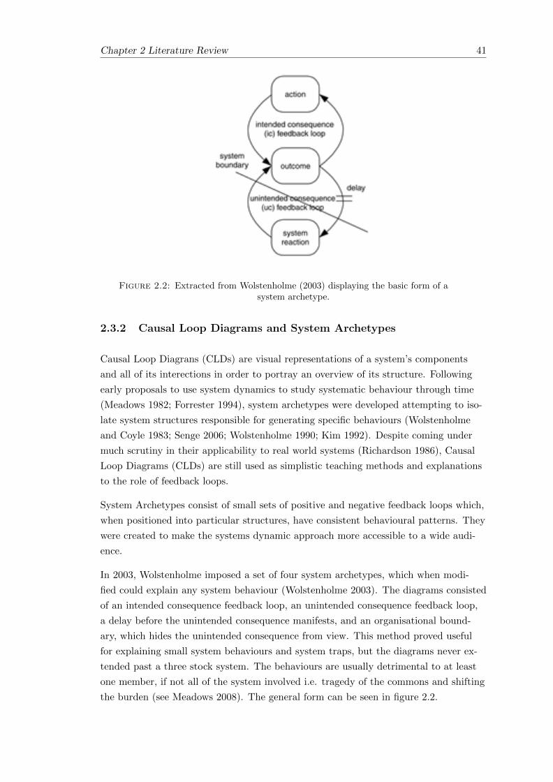
Chapter 2 Literature Review 41
Figure 2.2: Extracted from Wolstenholme (2003) displaying the basic form of asystem archetype.
2.3.2 Causal Loop Diagrams and System Archetypes
Causal Loop Diagrans (CLDs) are visual representations of a system’s components
and all of its interections in order to portray an overview of its structure. Following
early proposals to use system dynamics to study systematic behaviour through time
(Meadows 1982; Forrester 1994), system archetypes were developed attempting to iso-
late system structures responsible for generating specific behaviours (Wolstenholme
and Coyle 1983; Senge 2006; Wolstenholme 1990; Kim 1992). Despite coming under
much scrutiny in their applicability to real world systems (Richardson 1986), Causal
Loop Diagrams (CLDs) are still used as simplistic teaching methods and explanations
to the role of feedback loops.
System Archetypes consist of small sets of positive and negative feedback loops which,
when positioned into particular structures, have consistent behavioural patterns. They
were created to make the systems dynamic approach more accessible to a wide audi-
ence.
In 2003, Wolstenholme imposed a set of four system archetypes, which when modi-
fied could explain any system behaviour (Wolstenholme 2003). The diagrams consisted
of an intended consequence feedback loop, an unintended consequence feedback loop,
a delay before the unintended consequence manifests, and an organisational bound-
ary, which hides the unintended consequence from view. This method proved useful
for explaining small system behaviours and system traps, but the diagrams never ex-
tended past a three stock system. The behaviours are usually detrimental to at least
one member, if not all of the system involved i.e. tragedy of the commons and shifting
the burden (see Meadows 2008). The general form can be seen in figure 2.2.

42 Chapter 2 Literature Review
Generally causal loop diagrams are used for visual and structural data only (i.e. con-
nectedness or no. of feedbacks) while the shortfall of system archetypes is that the
small diagrams cannot guarantee to produce similar behaviour when built as part of
much larger systems. This happens because their connections to other loop systems
create interference with the associated behaviour.
2.3.3 Ford’s Behavioural Approach
Ford’s Behavioural Approach (Ford 1999b) is a systematic method which involves
the removal of individual loop structures at key stages of a system’s behaviour i.e.
around a behavioural change from exponential growth to decay. The more dramatic
the change of behaviour after the removal of a loop, the greater impact that loop is
assumed to hold at that point in time.
Ford’s loop deactivation method is tested by Keijser et al. (2012), concluding that it
requires further development on medium to large size models as the method quickly
becomes exponentially inefficient with model size.
2.3.4 Pathway Participation Metrics (PPM)
Pathway Participation Metrics was developed in 1996 by Mojtahedzadeh (Mojta-
hedzadeh 1997) and extended by Mojtahedzadeh in 2004 (Mojtahedzadeh et al. 2004).
The method is based on the works of Richardson (1984), identifying the significance of
loop polarity and loop dominance within dynamic systems.
Loop polarity works on the premise that a positive feedback loop represents a posi-
tive polarity and a negative feedback loop, a negative polarity. When multiple loops
interconnect, the system polarity is chosen by whichever loop holds dominance. As a
system changes through time, loop systems can undergo a change in dominance and
therefore, are capable of switching polarity.
Pathway Participation Metrics can be used to express whether a system’s behaviour
is dominated by positive or negative loops. PPM identifies dominant causal chains or
pathways within a system’s structure until it encounters a pathway which has already
been counted, in which case, it identifies a loop.
Unlike previous methods, PPM is able to follow a single variable through time, rather
than operating in the frequency domain. It also only identifies a single path of dom-
inance at any one time, therefore the PPM method does not account for model-wide
dynamics (Guneralp 2006).
Chapter 2 Literature Review 43
2.3.5 Eigenvalue Elasticity Analysis (EEA)
Eigenvalue Elasticity Analysis was first developed by Forrester (1982) for uses in eco-
nomic stabilisation policy. It is based on the idea that at any given time along a time
series, a system’s behaviour can be described through eigenvalues and eigenvectors,
once the model has been linearised. It has been developed from tools of modern linear
systems theory. EEA represents system models by converting them into matrix form
in a similar way to methods used in graph theory.
Eigenvalues represent behavioural modes (possible states of the system at a given
time), reflecting any changes which occur to the system. Perturbations of variables
which occur within the system’s structure which generate large changes in an eigen-
value have a high influence on the current behaviour. Perturbations which produce
small changes reflect a small change in eigenvalues and have little to no influence on
the current behaviour.
Guneralp (2006) describes how EEA can be used to reduce complex models to simpler
versions by eliminating structures which, while introduced during model construction,
make little or no contribution to behavioural output.
The elasticity of an eigenvalue λ is measured with respect to a gain parameter g, which
represents the strength of a connection, or link between two variables, in the form:
ε =∂λ
∂g.g
λ(2.1)
where g = the gain of each link and = the eigenvalues. The partial derivative ∂λ∂g
can be calculated algebraically using Mathematica as generally it handles the partial
derivative much better than Matlab.
This expresses the fractional change in the eigenvalue relative to the fractional change
of the link (Kampmann and Oliva 2008). Alternatively the influence of the parameter
can be measured with a dimension of 1/time and is therefore dependent on the time
scale units:
µ =∂λ
∂g.g (2.2)
Measuring the influence, rather than the elasticity is considered easier to interpret and
does not run into difficulties at low values of eigenvalue.
The Eigenvalue Elasticity method has been developed into multiple forms of use (EEA-
/LEEA/EVA). This means that the method can be determined by the projects re-
quirements and each method can overcome some of the downfalls posed by the others.
44 Chapter 2 Literature Review
2.3.6 Loop Eigenvalue Elasticity Analysis (LEEA)
Loop Eigenvalue Elasticity Analysis (LEEA) is a structural analysis technique which
identifies the influence of independent loop structures with respect to a system’s be-
haviour at any point in time. LEEA was developed by Kampmann (2012), who ex-
tended the work of EEA to monitor the influence of entire feedback structures. Using
the elements of a matrix J to store information, the strength, or ‘gain’ of any feed-
back loop in the model can be calculated as the sum of all link gain that connected
together to form that loop. A methodical breakdown of implementing LEEA can be
found in Guneralp (2006). Similar to EEA, interpretation of LEEA’s results must be
undertaken with care as eigenvalues do not relate to the observed behaviour of indi-
vidual variables.
A full explanation of the limitations of the LEEA technique, along with many solu-
tions to these limitations have been addressed by Guneralp (2006).
2.3.7 Eigenvector Approach (EVA) & Dynamic Decomposition Weights
Analysis (DDWA)
The eigenvector approach is an extension of the EEA/LEEA method and is the most
recent approach to be developed. DDWA improves on LEEA by considering how much
a change within an eigenvalue is weighted to an individual variable of the system.
As shown in Figure 2.3, extracted from Kampmann and Oliva (2008), it is the combi-
nation of eigenvalues and eigenvectors, which express the weighting of a behavioural
mode with respect to state variables.
In this combined method, eigenvalues show the behavioural modes and eigenvector
analysis provides the weights.
DDWA’s method involves a state element (a stock of the system) being assigned weights
coinciding with the extent to which it is affected by each eigenvalue. The sum of the
weights produces a weighted measure of that element’s overall significance (Guneralp
2006) as shown in Equation 2.3:
x(t0) = ω1λ1 + · · ·+ ωnλn (2.3)
Where x(t0) is the element’s significance, ωn is the weight of the behavioural mode
and λn is the behaviour mode. Guneralp (2006) extended this method by normalising
elasticity values of system elements to vary between -1 and +1. However, whether this
normalisation adds anything to the clarity of the method is questionable (Kampmann
and Oliva 2008).
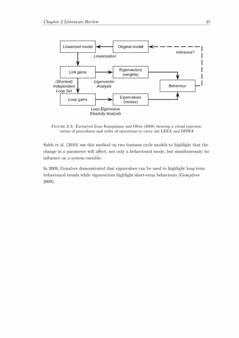
Chapter 2 Literature Review 45
Figure 2.3: Extracted from Kampmann and Oliva (2008) showing a visual represen-tation of procedures and order of operations to carry out LEEA and DDWA
Saleh et al. (2010) use this method on two business cycle models to highlight that the
change in a parameter will affect, not only a behavioural mode, but simultaneously its
influence on a system variable.
In 2009, Gonalves demonstrated that eigenvalues can be used to highlight long-term
behavioural trends while eigenvectors highlight short-term behaviours (Goncalves
2009).

46 Chapter 2 Literature Review
An
aly
tical
Tech
niq
ues
of
Syst
em
Dyn
am
ics
Ad
vanta
ges
Dis
ad
vanta
ges
2.3
.1T
rad
itio
nal
Contr
ol
Th
eory
•S
imp
leto
carr
you
t.
•E
asy
tote
ach
beg
inn
ers
ofsy
stem
sth
eory
.
•A
pp
lica
ble
only
tosi
mp
lesy
stem
sw
ith
very
few
vari
able
s.
2.3
.2C
au
sal
Loop
Dia
gra
ms
an
dS
yst
em
Arc
hety
pes
•E
ssen
tial
syst
emco
mp
onen
tsan
din
tera
ctio
ns
can
be
qu
ickly
rep
re-
sente
d.
•S
imp
le,
ofte
nuse
dfo
rco
nce
pt
bu
ild
ing.
•E
asil
yap
pli
cab
leto
teac
hin
gan
dex
pla
nat
ion
•C
LD
obsc
ure
sth
e′ s
tock
an
dfl
ow′
stru
ctu
reth
at
isco
mm
on
pra
ctic
ein
syst
emd
yn
am
ics
(Ric
hard
son
1986
).
•S
yst
emar
chet
yp
ed
iagra
ms
can
not
guar
ante
eto
pro
du
cesi
mil
ar
be-
hav
iou
rw
hen
inte
gra
ted
as
part
of
larg
ersy
stem
s.
•T
he
role
ofac
cum
ula
tion
inst
ock
sis
lost
asfe
edb
ack
stru
ctu
res
are
focu
sed
on.
•M
akes
no
dis
tin
ctio
nb
etw
een
info
r-m
atio
nli
nks
an
dra
te-t
o-l
evel
lin
ks,
crea
tin
gfa
lse
chara
cter
isati
on
of
pol
arit
ies
(Ric
hard
son
(1986))
.
•T
he
pos
itio
nof
org
an
isati
on
al
bou
nd
arie
san
dd
elay
sin
mu
chla
rger
syst
ems
are
hard
erto
de-
term
ine.
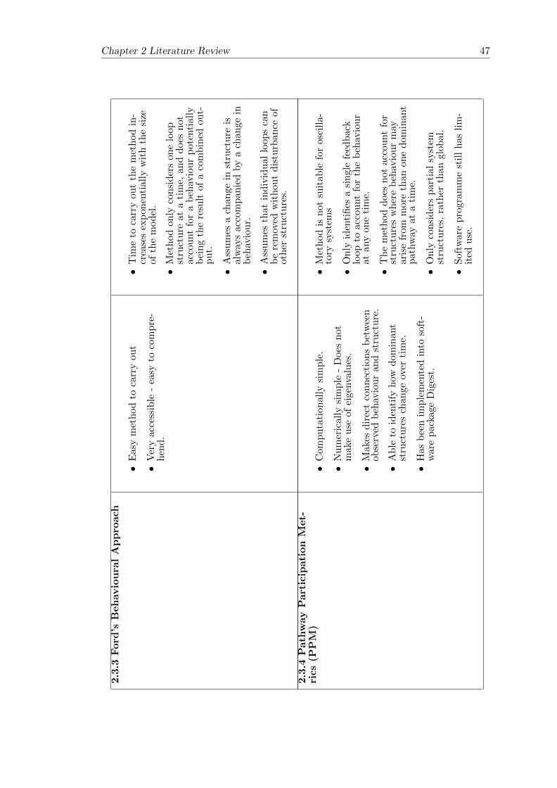
Chapter 2 Literature Review 47
2.3
.3Ford
’sB
eh
avio
ura
lA
pp
roach
•E
asy
met
hod
toca
rry
out
•V
ery
acce
ssib
le-
easy
toco
mp
re-
hen
d.
•T
ime
toca
rry
ou
tth
em
eth
od
in-
crea
ses
exp
on
enti
all
yw
ith
the
size
ofth
em
od
el.
•M
eth
od
on
lyco
nsi
der
son
elo
op
stru
ctu
reat
ati
me,
an
dd
oes
not
acco
unt
for
ab
ehav
iou
rp
ote
nti
all
yb
ein
gth
ere
sult
of
aco
mb
ined
ou
t-p
ut.
•A
ssu
mes
ach
an
ge
inst
ruct
ure
isal
way
sacc
om
pan
ied
by
ach
an
ge
inb
ehav
iou
r.
•A
ssu
mes
that
ind
ivid
ual
loop
sca
nb
ere
mov
edw
ith
ou
td
istu
rban
ceof
oth
erst
ruct
ure
s.
2.3
.4P
ath
way
Part
icip
ati
on
Met-
rics
(PP
M)
•C
omp
uta
tion
ally
sim
ple
.
•N
um
eric
ally
sim
ple
-D
oes
not
mak
eu
seof
eige
nva
lues
.
•M
akes
dir
ect
con
nec
tion
sb
etw
een
obse
rved
beh
avio
ur
and
stru
ctu
re.
•A
ble
toid
enti
fyh
owdom
inan
tst
ruct
ure
sch
ange
over
tim
e.
•H
asb
een
imp
lem
ente
din
toso
ft-
war
ep
acka
geD
iges
t.
•M
eth
od
isn
ot
suit
ab
lefo
rosc
illa
-to
rysy
stem
s
•O
nly
iden
tifi
esa
sin
gle
feed
back
loop
toacc
ou
nt
for
the
beh
avio
ur
atan
yon
eti
me.
•T
he
met
hod
does
not
acc
ou
nt
for
stru
ctu
res
wh
ere
beh
avio
ur
may
aris
efr
om
more
than
on
ed
om
inant
pat
hw
ayat
ati
me.
•O
nly
con
sid
ers
part
ial
syst
emst
ruct
ure
s,ra
ther
than
glo
bal.
•S
oftw
are
pro
gra
mm
est
ill
has
lim
-it
edu
se.
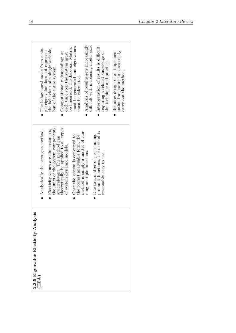
48 Chapter 2 Literature Review
2.3
.5E
igenvalu
eE
last
icit
yA
naly
sis
(EE
A)
•A
nal
yti
call
yth
est
ron
gest
met
hod
.
•E
last
icit
yva
lues
are
dim
ensi
onle
ss,
the
un
its
ofth
esy
stem
com
pon
ents
are
irre
leva
nt.
Th
em
eth
od
can
theo
reti
call
yb
eap
pli
edto
all
typ
esof
syst
emd
yn
amic
mod
els.
•O
nce
the
syst
emis
conve
rted
toth
eco
rrec
tan
alysa
ble
form
,th
em
eth
od
issi
mp
lya
mat
ter
ofru
n-
nin
gm
ult
iple
fun
ctio
ns.
•D
ue
toa
mat
ter
ofju
stru
nn
ing
pre
-bu
ilt
fun
ctio
ns,
the
met
hod
isre
ason
ably
easy
tou
se.
•T
he
beh
avio
ura
lm
od
efr
om
asi
n-
gle
eige
nva
lue
does
not
rep
rese
nt
the
beh
avio
ur
of
asi
ngle
vari
ab
le,
bu
tof
the
enti
resy
stem
.
•C
omp
uta
tion
all
yd
eman
din
g:
at
each
tim
est
epth
esy
stem
mu
stb
eli
nea
rise
d,
the
Jaco
bia
nM
atr
ixm
ust
be
gen
erate
dan
dei
gen
valu
esm
ust
be
calc
ula
ted
.
•A
nal
ysi
sof
resu
lts
get
sin
crea
sin
gly
diffi
cult
wit
hin
crea
sin
gm
od
elsi
ze.
•In
terp
reta
tion
of
resu
lts
isd
ifficu
ltre
qu
irin
ga
refin
edkn
owle
dge
of
the
tech
niq
ue
an
dp
ract
ice.
•R
equ
ires
des
ign
of
an
imp
lem
en-
tati
onfr
amew
ork
toco
nsi
sten
tly
carr
you
tth
em
eth
od
.

Chapter 2 Literature Review 49
2.3
.6L
oop
Eig
envalu
eE
last
icit
yA
naly
sis
(LE
EA
)•
Vis
ual
isat
ion
oflo
opin
flu
ence
over
tim
ep
rod
uce
das
a(s
emi-
)con
tinu
ous
grap
h.
•E
nco
mp
asse
sth
een
tire
feed
bac
kst
ruct
ure
aton
cean
dac
cou
nts
for
all
syst
emei
genva
lues
.
•S
hor
test
Ind
epen
den
tL
oop
Set
(SIL
S)
pre
sents
opti
mis
tic
grou
nd
sfo
rru
nn
ing
LE
EA
onla
rge
syst
emm
od
els.
•S
ame
adva
nta
ges
asE
EA
(Sec
tion
2.3.
5)
•U
seof
ab
stra
ctm
ath
emati
cal
ter-
min
olo
gy
(eig
enva
lues
&ei
gen
vec-
tors
).
•T
he
inab
ilit
yto
iden
tify
stru
ctu
ral
infl
uen
ceon
ind
ivid
ual
state
vari
-ab
les.
•E
igen
valu
esca
nex
pre
sssi
mil
ar
lev-
els
ofd
om
inan
cesi
mu
ltan
eou
sly,
red
uci
ng
on
e’s
ab
ilit
yto
spec
ify
an
ind
ivid
ual
beh
avio
ura
ld
rive
r.
•T
he
ab
ilit
yto
inte
rpre
tre
sult
sb
e-co
mes
diffi
cult
as
agre
ate
rnu
m-
ber
of
vari
ab
les
are
ad
ded
toth
em
od
el.
2.3
.7E
igenvecto
rA
pp
roach
(EV
A)
&D
yn
am
icD
ecom
posi
tion
Weig
hts
An
aly
sis
(DD
WA
)•
Wh
enco
mbin
edw
ith
LE
EA
,D
DW
Ais
cap
able
ofre
lati
ng
the
infl
uen
ceof
loop
stru
ctu
res
toin
di-
vid
ual
vari
able
s.
•M
ajo
rity
ofth
ew
ork
isac
hie
ved
thro
ugh
fun
ctio
ns.
•E
igen
vect
ors
can
not
pro
vid
ea
stan
-d
alon
em
eth
od
for
loop
dom
inan
ceas
they
are
not
calc
ula
ted
as
afu
nct
ion
of
loop
gain
s.
•G
ener
al
EV
Am
eth
od
enco
unte
rsis
sues
wit
hosc
illa
tion
s,si
mil
ar
toP
PM
(sec
tion
2.3
.4).
•R
equ
ires
the
syst
emto
be
lin
-ea
rize
dat
each
tim
est
ep.

50 Chapter 2 Literature Review
2.3.8 An Analysis Best Suited for Structural Analysis of Dynamic
Systems
Each technique reviewed within this section has the capability to increase the knowl-
edge and understanding gained from a system’s model. However, the extent to which
novel information can be gained and the potential of the application can vary heav-
ily between techniques depending on the properties of the model system and what the
project requires.
From the seven analysis techniques listed above, Causal Loop Diagrams (CLD), Loop
Eigenvalue Elasticity Analysis (LEEA) and Dynamic Decomposition Weights Analysis
(DDWA) have been selected as three techniques to pursue and assess for the advance-
ment of SES models. The most recently developed technique is a combination of Loop
Eigenvalue Elasticity Analysis (LEEA) and the Eigenvector Approach (EVA) (Kamp-
mann and Oliva 2006, Kampmann and Oliva 2008). Collectively these techniques fo-
cus on feedback loops as endogenous drivers of system behaviour and allow the user
to investigate the influence of loop structures on individual state variables (stocks) as
they change through time.
Among all of the structural analysis techniques reviewed, LEEA removes the ‘trial and
error’ component to identify influencial loops which are used by many of the other
techniques. This means LEEA is efficient, especially when the system structure changes
between design iterations or between simulations.
With the primary focus on LEEA, this work will conduct a meta-analysis of structural
loop analysis across all stages of model design, implementation, output and applica-
tion to policy. LEEA will be explored in the context of model construction alongside
causal loop diagrams (CLDs) and in the context of policy design and implementation
alongside DDWA.
2.3.9 Comments & Reflections
Kampmann and Oliva (2008) state that for policy analysis, both the eigenvalue and
eigenvector approach will need to be used. Kampmann and Oliva (2008) states that
we will “always have to rely on simulation to discover the dynamics implied by a struc-
ture.” However, we can aim for the identification of dominant structures within mod-
els to focus our efforts, such as key feedback loops and links.
Saleh et al. (2010) describes the danger of falsely allocating behaviours to the wrong
feedback mechanisms. Intervention of a system after the misinterpretation of a feed-
back mechanism could create no impact at all, wasting valuable time and resources, or
worse, drive a system to collapse at a faster rate.

Chapter 2 Literature Review 51
The following example illustrates the dangers of misunderstanding the mechanisms at
play within a system:
In the Yunnan Province, China, regional agriculture was increased to support the de-
veloping population and migration into the area requiring a greater amount of food.
To increase output, farmers occupied more land for agriculture and were allowed to
use more fertilizer. Misunderstanding the feedback mechanisms at play within the
nearby lake, the excess nutrients, applied over a series of decades, caused the local
lake to turn eutrophic, crippling the fishing and tourist industry of the region and ul-
timately leading to mass human migration away from the area. The critical transition
which occurred was investigated by Wang et al. (2012).
LEEA, and other structural analysis techniques have only been used on small ecolog-
ical models to act as examples of the technique’s progression or to investigate small
agricultural practices (Bueno 2012, Bueno 2013). Despite being shown as highly ap-
plicable to socio-ecological systems, structural analysis techniques have yet to be used
extensively or see common practice within the field. Many behaviours known to act in
SESs (i.e. tipping points, overshoots, oscillations, flickering, and critical slowing down,
as shown in Scheffer (2009) & Wang et al. (2012)) have not been explored using struc-
tural analysis, despite acknowledging the multitude of feedback mechanisms at play.
In 2012, N. P. Bueno contributed to bridging this gap, aiming to find a common prac-
tice of measuring degrees of resilience through system dynamics and dominant loop
polarity investigation. Bueno (2012) states that if the behaviour of a low resilience
system is dominated by a feedback loop, then small changes in the strength of that
loop can lead to large changes in the system’s behaviour and therefore stability.
2.3.10 Personal communications with Prof. C. E. Kampmann (2015)
Professor. C. E Kampmann is one of the early developers and testers of Loop Eigen-
value Elasticity Analysis along with its multiple counterparts, EEA & DDWA. In the
early stages of applying LEEA to ecological system models, a conversation was held
with Professor Kampmann to discuss the technique’s capabilities and whether there
was any merit to applying LEEA to other worldly systems, other than the industrial
and business models which it had been applied to previously. This section highlights
extracts from that conversation and the initial afterthoughts. The content within this
section is based on the opinions and experiences of Prof. Kampmann. This section has
been separated from the main content of the literature review as the points made have
not been established from peer review material, despite this, the experience of Prof.
Kampmann is considered a valuable asset when determining the applicability of LEEA
to the socio-ecological field.
Discussion point 1: Concerning dynamic behaviours

52 Chapter 2 Literature Review
In Kampmann and Oliva (2008), three system models of varying sizes and dynamics
were analysed using LEEA in order to access the application of structural loop anal-
ysis to varying business models. To lead on from the information gained from that
study, one of the initial questions posed during personal communications with Prof.
Kampmann was what models and system dynamics he found LEEA analysis most
applicable to in terms of information gained and understanding of the system. Prof.
Kampmann’s response has been summarised:
“. . . where the analysis really shines is where the system has some kind of oscillatory
mode going on, or systems where there is a single transient.”
Prof. Kampmann then gave Limits to Growth by Meadows et al. (1972) as an exam-
ple of a system which is capable of experiencing an overshoot, a collapse or a tran-
sition between states. This part of the conversation gave great promise to the appli-
cation of LEEA to socio-ecological systems. Without prompt or mention of socio-
ecological systems, Prof. Kampmann mentioned multiple dynamic behaviours that
elicit large topics of discussion within the SES community. Many systems of SES are
speculated for their ability to experience multiple stable states, with overshoots and
collapses being common dynamics in population growth and ecosystem services.
With this in mind, the prospects of using LEEA in conjunction with SESs seemed
positive. The question which naturally follows is what utility or additional value can
the technique bring to systems which experience these behavioural dynamics? Lim-
its to Growth is a reasonably simple model to understand as the properties of the
model which cause it to undergo collapse and overshoots are well known. For LEEA
to be considered as an appropriate analysis tool to SESs, it must be capable of adding
to our existing knowledge of the systems dynamics within a socio-ecological context.
From this section of the conversation one of the main aims of the thesis was formu-
lated: Is LEEA able to provide us with novel information about our system’s dynamic
behaviours through the analysis of system structure?
Discussion point 2: Models where LEEA may be inapproariate
Prof. Kampmann expressed that in his experience the utility of the method (mean-
ing LEEA) depends on the kind of system that you are dealing with. Systems which
express chaotic behaviour will show little information in the output of the analysis as
the analysis output will be just as complex to understand as the output of the model
itself.
It must be accepted that this analysis will not always be appropriate for every sys-
tem. The utility and information the analysis is able to provide will largely depend on
the complexity, size and internal dynamics of the model. On the reverse side of model
complexity, if the model system is relatively simple and well known, then loop anal-
ysis may not offer any new insight. Systems which are relatively simple, for example
Chapter 2 Literature Review 53
only carrying two stocks with very few feedback mechanisms can often be investigated
using simple graph theory or using system archetypes. Other systems where this tech-
nique will not be appropriate are those whose stocks variables are not included as part
of multiple loops as their dynamics will not be accounted for within the Jacobian ma-
trix, where each cell represents an interaction between two stocks. Models which in-
clude stock-less feedback loops may have to be reconfigured structurally, or the in-
fluence and elasticity outputs of the analysis may not accurately represent the entire
loop set, therefore highlighting a disadvantage of this technique.
Discussion point 3: Future development of the method
The third section of the discussion overviewed the general accessibility of LEEA, where
it currently stands in development and limitations of the technique which Prof. Kamp-
mann was particularly aware of. The accessibility of LEEA was of high concern when
attempting to introduce LEEA to an entirely new field of research. Current socio-
ecological studies do not utilise LEEA: not only is the analysis tool an unfamiliar
one to the field of SES, but SES research does not inherently involve system dynamic
modelling or involve in depth knowledge of feedback loops and their ability to drive
system behaviour.
Prof Kampman’s response on this issue stressed that LEEA as an analysis tool is still
within its infancy and is still undeveloped as a method. In order to be capable of car-
rying out LEEA and fully appreciate the results, there is base level of mathematical
foundation required. To get the most out of LEEA, it is helpful to have at least a
basic understanding of system dynamic models and how to manipulate/extract data
from them, linear stability theory, graph theory and feedback loop behaviour. While
this may seem like a daunting process to a new user, Naumov & Oliva (2017) have de-
veloped online tools and software packages to help streamline the process. While some
manual data manipulation and basic understanding of Jacobian matrices and eigen-
values is required in order to understand the information LEEA outputs, many of the
calculation steps are taken care of within packages run through Mathematica and are
in open access, available online.
Regarding analysis development and what was known of the technique, Prof. Kamp-
mann inferred that there were still unsettled questions surrounding LEEA’s capabil-
ities and what niche it could occupy with future development. It is known that one
of the main limitations of LEEA is its ability to be applied to large complex models,
as the data produced by the analysis becomes increasingly as large and convoluted
to interpret. The extent to which LEEA’s application is still considered practical and
useful is unknown. At the current stage in LEEA’s development, the best method for
discovering its uses and its limitations is just to try it and test it.
To a new user wishing to explore and utilise LEEA as part of their research there is
an inherent risk of using pre-developed software for an analysis which is in its relative

54 Chapter 2 Literature Review
infancy. Attempting to use Naumov and Oliva’s software packages without first learn-
ing the basic theory and steps involved in carrying out LEEA risks treating the cal-
culations as A) gospel and B) ‘black box’ and thus losing a lot of information. Infor-
mation gained from LEEA is obtained from multiple sections throughout the analysis
process and is not all concentrated as a single output, although this could be a direc-
tion to take LEEA in order to make the processing more streamline and accessible.
Afterthoughts
LEEA has already been used successfully and shown to provide novel information to
system models surrounding business and industry. With LEEA’s strengths and most
noteworthy application to systems which are prone to oscillations, critical transitions
and collapses, there is also a great deal of potential for LEEA to help us understand
more about our human-environment interactions which are recorded to experience
these dynamic behaviours all the time. LEEA could bring an alternative way to study
structural drivers of our socio-ecological models. In order to find its niche amongst
current analysis tools, if it has a place at all, it must first be tried and tested in a va-
riety of system models, which cover a wide range of sizes, dynamics and represent a
multitude of real-world systems. While this requirement and amount of testing is too
great a feat to achieve in one thesis, one can, for want of a better phrase, get the ball
rolling. In light of this, this thesis takes an initial look at LEEA in the context of SES
models. An overview of LEEA’s methodology and how to carry it out is provided as-
suming little to no prior knowledge of system dynamics or structural analysis. LEEA
is critiqued for its current accessibility, utility, limitations and what it could bring to
an SES study.
2.4 Model and Analysis Validation
Validation in the context of ecological modelling refers to the extent that a model
is fit for purpose to the job and initial goals for which it was designed. In order to
achieve model validation, the user must first have decided upon: 1) the purpose of the
model, 2) the performance criteria and 3) the context of the model (Rykiel Jr 1996).
Validation is then split into operation, theory and data, where validation can be un-
dertaken to the operation and data parts of a model and simulation, but not on the
theory (Rykiel Jr 1996).
Rykiel Jr (1996) emphasises that the most common downfall of ecological model val-
idation occurs with failure to state what the validation criteria are to be. Stating the
validation criteria of a model is critical as there are no universal standards when it
comes to modelling the environment. The most common validation criterion chosen is
to be able to match simulation output with observed data, otherwise known as the
’goodness of fit’. Richardson and Pugh III (1981) enforce the idea that validation

Chapter 2 Literature Review 55
should be a continuous effort to build confidence within the model and not simply a
task that must be undertaken as a stepping stone between model completion and pol-
icy analysis.
The ‘goodness-of-fit’ approach is a validation technique used as a correlation based
measurement between simulation and data and has been applied to multiple ecological
models, notably for hydrologic and hydroclimatic modelling with limited use (Legates
and McCabe Jr 1999). Alternative approaches include coefficient of efficiency and in-
dex of agreement which are reportedly able to cover many of the limitations found
when conducting correlation based measurements (Legates and McCabe Jr 1999).
The original goodness of fit approach is called the Coefficient of Determination. This
describes the proportion of variance within the real-world data set which can be ex-
plained by the model. The Coefficient of Efficiency and Index of Agreement both make
use of a parameter known as the ratio of mean square error, where higher values indi-
cate a better agreement between the model and observed data variance (Wilcox et al.
1990; Willmott 1981).
The ‘goodness-of-fit’ approaches provide model validation to an extent, but their abil-
ity to estimate and calibrate model performance does not guarantee a models abil-
ity to predict future events (Power 1993). If the purpose of a model is to be used for
prediction then it can be compared and contrasted against other models built for the
same purpose for statistical adequacy. Statistical adequacy stems from econometric
and statistical forecasting literature and involves the use of a statistical checklist to
rank the properties of a model (Power 1993).
Another form of model validation stems from a statistical comparison of a model’s
multiple predictions against measurements of a system’s real world behaviour. This
uses the hypothesis of ‘no difference’; a null-hypothesis that the model is acceptable
(Robinson and Froese 2004). A null-hypothesis is a statistical test with the hypothesis
that there is no significant difference between a model’s output and the observed data
set with any variations being due to sampling or experimental error alone. Robinson
and Froese (2004) work on an empirical forest growth model and use an approach
known as the hypothesis of dissimilarity, a null hypothesis that the model is unaccept-
able, arguing that it is a more robust measurement of model validation.
2.4.1 Validation of LEEA and its outputs
In the context of validating LEEA, system dynamic models are used less for prediction
purposes and more for simulation and scenario comparison, leaning on the strengths of
system dynamic modelling which focus on system structure and behavioural trends,
rather than specific output values. Validation can come in the form of an iterative

56 Chapter 2 Literature Review
process comparing model simulation to observable data, much like ‘goodness-of-fit’ ap-
proaches. However, this is for validation of the model, but not of the outputs of LEEA
analysis itself.
Validation of LEEA’s outputs comes in two parts, an internal validation and an ex-
ternal validation. The internal validation is a reflection of LEEA being a purely ana-
lytical technique with a set procedure to follow, meaning that its output is completely
reliant on the structure, dynamics and values assigned to a model. LEEA’s internal
validation is therefore only as good as the validity of the model it is being used on.
External validation takes into account whether the information LEEA produced re-
garding feedback loop dominance is reflected in real world feedback mechanisms. This
would require the ability to manipulate leverage points and feedback loops within the
real world system to see if LEEA’s outputs are reliable. If LEEA identifies a highly
influential loop structure within the model, but upon manipulation of the real world
system, nothing changes, it could mean there is a disconnect between the real world
system and the structure or dynamics of the model LEEA is being used to analyse.

Chapter 3
Methodology
3.1 Loop Eigenvalue Elasticity Analysis (LEEA)
Loop Eigenvalue Elastcity Analysis is used throughout and is integral to the material
within each chapter of this thesis. The following chapter is a breakdown of LEEA’s
methodology. Almost all calculations regarding LEEA and generating its output have
been automated (Naumov & Oliva 2017), yet it is important that at each step of the
methodology, what is being calculated and why, is understood, in order to make in-
formed interpretations of the results.
Loop Eigenvalue Elasticity Analysis (LEEA) was developed in 1996 by Kampmann
(2012) who extended the works of Forrester (1982) regarding Eigenvalue Elasticity
Analysis (EEA) from 1982-1983. While the premise of using system eigenvalues to de-
scribe the behaviour of a linear system was well established in classical control theory,
N.B. Forrester was the first to use this method on system dynamic models to develop
notions of eigenvalue elasticity and link them to model parameters ( Forrester 1983,
Forrester 1982). Eigenvalue elasticity was a way to measure the relative change occur-
ring to a system eigenvalue with respect to a relative change to a system parameter.
Forrester used this technique primarily in economic stabilization policy. Kampmann
(2012) extended the theory behind EEA, allowing for entire feedback loop structures
to be compared against the system’s eigenvalues and thus formed the basis for LEEA.
EEA and LEEA were initially very manually intensive, taking a lot of preparation
time before any computer simulations could be run. LEEA was later extended and
made to be more automated (Kampmann 2012, Guneralp 2006, Kampmann and Oliva
2006), with the entire process being made much simpler, more automated and user
friendly in recent years (Naumov & Oliva 2017, Oliva 2015). Structural Loop analy-
sis has been used extensively on economic and industry modelling as well as to simply
expand the capabilities and accessibility of the technique (Saleh et al. 2010, Guneralp
2006, Kampmann and Oliva 2006, Guneralp et al. 2005).
57

58 Chapter 3 Methodology
Loop Eigenvalue Elasticity Analysis uses system dynamic theory (Forrester 1971),
where a system can be represented as a series of stocks and flows, based on the idea
that a system’s behaviour is driven by properties of its internal structure (Forrester
2007a). LEEA identifies a set of feedback loops within a system’s structure known as
the Shortest Independent Loop Set or SILS (Kampmann 2012, Goncalves 2009, Oliva
2004), which are collectively responsible for driving the system’s behaviour. LEEA
then structurally analyses the loop set, identifying which feedback loops are dominat-
ing the system’s behaviour at any point in time.
LEEA is based on the ability to describe a system’s behaviour through a set of eigen-
values at any point along that system’s time series and link them to the driving be-
haviour of feedback loops of the system’s internal structure. The approach is taken
from linear theory and is applied to non-linear systems by linearizing the system at
every point in time (Goncalves 2009). Each eigenvalue of the system represents a sin-
gle behavioural mode which reflect the behaviour patterns of the system. Perturba-
tions which occur within the system’s structure (i.e. the system’s feedback loops) are
able to generate changes within the eigenvalues. Perturbations from feedback loops,
which create large changes to an eigenvalue indicate high influence on the current be-
haviour, while perturbations which produce small changes to an eigevalue indicate lit-
tle to no influence on the current behaviour. LEEA is able to identify how much an
individual feedback loop is dominating the current system behaviour, thus allowing
the user to identify a hierarchy of loop dominance at any point in time.
Despite multiple sources expressing the benefits that the LEEA technique can bring
to an understanding of system behaviour (Guneralp et al. 2005, Kampmann and Oliva
2008, Kampmann 2012) and several attempts to make the technique more accessible,
(Naumov & Oliva 2017, Oliva 2015, Guneralp 2006) the method has only seen lim-
ited use in the field of socio-ecological systems (Lade and Niiranen 2017, Bueno 2012,
Bueno 2013). The purpose of this initial study is to assess the benefits and limitations
which LEEA can bring to the field of socio-ecological and complex ecological mod-
elling, with a focus on, but not limited to, systems able to undergo rapid regime shifts
between stable states.
Calculating Loop Elasticities and Influence values is a step process to which the fol-
lowing must be calculated:
1. Constructing Differential Equations (3.1.1)
2. Jacobian Matrix of the system dynamic model (3.1.2)
3. Eigenvalues of the Jacobian matrix (Behavioural modes) (3.1.3)
4. Identifying the feedback loops in the Shortest Independent Loop Set (SILS)
(3.1.4)

Chapter 3 Methodology 59
5. Loop gains (3.1.5)
6. Loop Eigenvalue Elasticity (3.1.6)
7. Loop Influence (3.1.7)
3.1.1 Constructing Differential Equations
A key step in the process of determining system eigenvalues, required for LEEA and
the comparison to system feedback loops is the generation of a system’s Jacobian ma-
trix. The Jacobian matrix requires the system to be described as a set of differential
equations. In order to produce analytical differential equations, all variables must be
in analytical form.
System models developed using system dynamics are often created using a set of pre-
determined differential equations which describe the behaviours expressed by the sys-
tem. This can often be the case in ecology and socio-ecology where dynamic behaviours
i.e. populations growth or system collapse, have well establised analytical formulae
associated with them. In many other cases, system dynamic models are not created
using predetermined formula and are built from a foundation of model components
and simple interactions, built up through multiple model iterations. In either circum-
stance, it is possible to use the form of a system dynamic model to gain a set of differ-
ential equations which describe the system.
In order to construct differential equations from a system dynamic model (sometimes
referred to as a stock and flow model), the components of the model must first be
categorised into its stocks, flows, auxiliary variables and constants. Each stock vari-
able represents a separate differential equation used to describe the model system,
i.e. three model stocks infers that the system can be described using three differential
equations. From this, each stock variable is expanded to represent its inputs and out-
puts. Below is a very simple example of equating a system dynamic model stock to a
differential equation. Any input of a stock corresponds to an addition (+) in its differ-
ential equation form and any outputs of a stock represent a subtraction (-). Examples
can be seen below in figure 3.1.
Figure 3.1: A visual respresentation of a stock variable (black box), its flows(double lined black arrows), sources and sinks (cloud shapes). The image is ex-tracted from a Vensim model and translates to the following dynamical equation:
δISδt = newindustries− demolition

60 Chapter 3 Methodology
3.1.2 The Jacobian Matrix
The structure of any linear system model can be represented within a square, ‘nxn’
matrix (Saleh et al. 2005). The Jacobian matrix or ‘Gain Matrix’ is a representation
of all the links between every stock in a system in their most compact form (Guner-
alp et al. 2005). The Jacobian is equivalent to writing down each differential equation
of a system and taking the partial derivatve of each with respect to each stock of the
system while all other variables are treated as constants. Each partial derivative gen-
erated equates to one entry or one coefficient of the Jacobian Matrix. Each element of
the matrix represents how one stock affects another’s trajectory (i.e. how it changes
over time), when all other stocks are kept constant.
The Jacobian Matrix can also be referred to as the Gain Matrix because its entries
are made up of the ’gains’ of the links that exist between stocks. The concept of link
gains and loop gains are expanded upon in section 3.1.5 entitles ’Loop Gains’.
To calculate the Jacobian Matrix, the differential equations for each stock of the sys-
tem must be known. A Jacobian Matrix takes the generalised form:
J =
∣∣∣∣∣∣∣∣∂x1∂x1
. . . ∂x1∂xn
.... . .
...∂xn∂x1
. . . ∂xn∂xn
∣∣∣∣∣∣∣∣ . (3.1)
Where x represent stocks, x represents the rate of change of that stock or δxδt and n
represents the number of stocks. So x2 refers to the second stock of the model. Note it
does not matter which number is assigned to which stock so long as the order is kept
consistent. Each entry of the Jacobian, i.e. ∂xi∂xj
represents the change in net rate of
stock variable i as a response to an infintesimal change in the value of stock variable j
(Saleh et al. 2005).
The calculation of a Jacobian matrix requires the system to be linearised. By calculat-
ing the entries of the matrix at any point in time, all non-linear inputs can be taken
as constants and the model can be linearised at that individual point in time (Kamp-
mann 2012; Guneralp 2006; Forrester 1983). If the model is to be linearised at each
time step, then the time steps or changes in the system between time steps, must be
very small to assume linearity. “... the dynamics of the original model can be approxi-
mated through time by the behaviours of a series of linear models with varying entries
in their gain matrix” (Guneralp et al. 2005, Guneralp 2006).
While the Jacobian Matrix can be calculated by hand, it can often get extremely com-
plex, especially as systems get larger and stock number increases. Key functions in
Matlab or Mathematica for this procedure include ’jacobian ([f(x),f(y)],[x,y])’, eig(J)
and subs(e) for the creation of the Jacobian matrix, its eigenvalues and substitution

Chapter 3 Methodology 61
of data into those eigenvalues. The calculation of the Jacobian Matrix is done auto-
matically within LEEA’s online support material (Naumov & Oliva 2017), but it is
calculated in the background code and is not seen by the user.
3.1.3 Calculating Eigenvalues
Eigenvalues are calculated from a system’s Jacobian matrix and are an integral part of
interpreting LEEA’s output and the calculation of loop eiegnvalue elasticity. Since the
Jacobian is an nxn matrix, were n is equal to the number of stocks in the model, the
number of eigenvalues of a system is equal to the number of stocks in that system.
Eigenvalues are a set of scalars associated with the linear system equations and pro-
vide valuable insight into the properties of the Jacbian matrix. Eigenvalues have mul-
tiple uses across different fields (i.e. mechanical engineering, image processing, physics),
but they are used in linear systems as they have a common application for stability
analysis. Generally eigenvalues are able to characterise the underlying linear transfor-
mations of a system’s behaviour in a much simpler manner than n2 entries of a square
matrix (Saleh et al. 2010).
Eigenvalues (λ) are calculated for an nxn matrix (J) by satisfying the equation: det(J−λI) = 0, where I is an nxn identity matrix. From linear stability theory, eigenvalues
can be used to determine if a system at a fixed point is stable or unstable (Glendin-
ning 1994). Eigenvalues are capable of being real, or complex numbers with a real and
imaginary part. If the real part of all eigenvalues are negative, then the fixed point is
stable. If the real parts of any of the eigenvalues positive, then the fixed point is un-
stable. The properties of these eigenvalues tell us a lot about what kind of behaviour
the system will be expressing:
• If λ = Positive and real: system is expressing exponential growth.
• If λ = Negative and real: system is expressing exponential decay.
• If λ = complex conjugate (has a real and imaginary part) with a positive real
part: system is expressing oscillations which are expanding.
• If λ = complex conjugate with negative real part: system is expressing oscilla-
tions which are dampening.
Like the majority of steps required for LEEA, many of the calculations are automated
within Naumov & Oliva (2017). Otherwise, the calculation of eigenvalues can largely
be achieved through pre-existing functions available in software such as Matlab or
Mathematica. Using eig(J) Matlab can calculate the eigenvalues for a matrix J . The

62 Chapter 3 Methodology
software is capable of calculating eigenvalue with algebraic symbols which can then be
substituted for time-series data.
Prioritising Eigenvalues
Eigenvalues are prioritised during the interpretation of LEEA in order to filter out
much of the enormous amount of data it is capable of producing which is not relevant
to the questions and goals of a project. Since the choosing of eigenvalues and interpre-
tation of loop influence plots is not an automated procedure and must be conducted
by the user, it is the part of the analysis which can be the most time consuming. The
following provides a short guide on how to choose eigenvalues that should be focused
on during LEEA. An example has been provided to help illustrate this procedure.
The eigenvalues which should be focused on are based on three properties which should
be prioritised in the following order:
1. Are any eigenvalues positive?
Positive eigenvalues are associated with runaway, exponential and destabilizing
behaviour. They indicate that a system is unstable, capable of transitioning
away from their current state with only a small perturbation. Feedback loops
dominating in positive eigenvalues can therefore represent long term behavioural
trends in a system such as exponential growth or decay that takes time to build
up. To that end, positive eigenvalues which hold relatively small magnitudes can
be as, if not more important to focus on than negative eigenvalues with rela-
tively large magnitudes.
2. Which eigenvalues hold the highest magnitudes?
Eigenvalues which hold high magnitudes relative to other eigenvalues are seen
as having more representation over the system’s current behaviour. High mag-
nitude, negative eigenvalues represent a steeper and faster pull of a system back
to a stable state compared to low magnitude, negative eigenvalues. High mag-
nitude, positive eigenvalues represent a steeper, faster pull away from a stable
state compared to small magnitude, positive eigenvalues.
Eigenvalues which hold relatively similar magnitudes must be compared against
each other simultaneously in order to determine highly influential loops. The
loop influences values associated with two different eigenvalues can often differ
greatly, even when the eigenvalues hold a similar magnitude and the same polar-
ity. When this occurs, dominant feedback loops within both eigenvalues should
not be ignored, remembering that eigenvalues represent different long term and
short term behaviours of a system. The dominant feedback loops across the dif-
fering eigenvalues will be representing alternate behaviours across potentially dif-
ferent timescales. The user should primarily go back to the variables, values and
Chapter 3 Methodology 63
the equations of the interactions within those feedback loops in order to work
out why the feedbacks are simultaneously registering as highly influential, but
for different short term/ long term behaviours.
3. How are the eigenvalues changing through time?
While the priority for choosing eigenvalues should consider the polarity and
magnitude at individual points in time because that is how the analysis lin-
earizes the model, the user should not completely ignore the trajectory of an
eigenvalue as it changes through time. Eigenvalues which become progressively
less negative may be indicative of behaviour within the system generating a de-
creasing amount of stability. Eigenvalues which sit at zero or are primarily neg-
ative may transition into positive values, where they must now be prioritised for
information regarding the system’s long term behaviours.
The best scenario is if a user is able to keep track on loop influence values associated
with every eigenvalue of a system. However, this is often not practical if there are a
high volume of eigenvalues and feedback loops and often not necessary if many of the
eigenvalues hold relatively low magnitudes for the entire simulation.
If an eigenvalue is a complex number with real and imaginary parts, separate the two
into different plots. Primarily use the real part to determine which eigenvalues to
prioritise, but use the imaginary part to identify complex conjugate pairs and to ac-
knowledge when the system is expressing oscillatory behaviour, rather than exponen-
tial or dampening behaviours.
When eigenvalue plots begin to look complicated, usually due to a high number of
stocks being present in the system and some interesting dynamic behaviours occur-
ring, the best thing to do is to break the output down into sections. An example has
been selected to showcase how a user might go about interpreting an eigenvalue plot:
First things to note: 1) The system has seven eigenvalues. 2) The eigenvalues are com-
plex numbers (this example will focus on the real part). 3) The system appears to
undergo some cyclic behaviour shown by the periodic spiking of eigenvalue 1. 4) The
eigenvalues change constantly throughout the time line, choosing which to prioritise is
not a trivial process.
Since there is no clear eigenvalue to focus on, the user’s best option is to break the
plot into sections (Figure 3.3).
Now examine each section separately. While this may be a time consuming process,
it will ensure the most understanding about the system across each point within the
simulation. If the sections are inspected in the order in which they occur it may be
easier to explain transitions and changes between sections which reflect in the system’s
overall behaviour.

64 Chapter 3 Methodology
Figure 3.2: An eigenvalue plot produced from LEEA of a seven stock system.Each line represents a different eigenvalue of the system as it changes through the
simulation.
Figure 3.3: An eigenvalue plot of a seven stock system sectioned into managableparts fo analysis.
Section A:
• Section A appears not to follow the cyclic behaviour of the rest of the model
simulation and so might be a remnant of model spin-up, largely being able to
be ignored, otherwise
• Eigenvalue 3 holds the highest magnitude positive value which should be priori-
tised as a reflection of instability within the system, while eigenvalues 2 and 1
should be inspected for sources generating stability.

Chapter 3 Methodology 65
• Note that despite loop 3 holding a high positive value relative to loops 4-7 which
are sitting closer to zero, the value of eigenvalues 2 and 1 still hold higher nega-
tive magnitudes so should not be ignored.
Sections B, D and F:
• These sections are the most complex of the time series.
• Each holds a relatively high negative eigenvalue which should be inspected for
feedback loops generating stability within the system.
• Multiple eigenvalues appear to cross into positive values, but their trajectories
change a lot within the section. Here the best thing to do for each of these sec-
tions is to plot each time section separately, potentially not plotting eigenvalue 1
so that a closer inspection of dynamics around zero can be achieved.
• The eigenvalues around zero all appear to hold relatively similar influences, so
any which cross into positive values should be inspected for sources of instability.
• Feedback loops generating instability within these sections should be compared
against those in eigenvalue 1, especially in the knowledge that eigenvalue 1 is
about to spike into high positive values.
Sections C, E and G:
• These sections are much simpler to process. Eigenvalue 1 dominates these sec-
tions with relatively high spikes in positive values and so can be prioritised for
inspection over all others.
• Note Feedback loops responsible for the exponential build up from the previous
sections of these spikes.
• Be sure to actively compare loop influences within this eigenvalue against the
spike. Do the loop influences spike at the same time and do some drop in magni-
tude in respect to the spike?
The interpretation of eigenvalues and feedback loop influences will always bring new
challenges for interpretation of LEEA with each new model it is used upon. The best
practice is to follow a structured guide such as the three steps mentioned above in or-
der to maintain consistency and to acknowledge that careful interpretations can take
time, but are often worth the extra understanding that is gained over the systems dy-
namics and behaviour.

66 Chapter 3 Methodology
3.1.4 Identifying the feedback loops in the Shortest Independent
Loop Set (SILS)
LEEA requires all individual feedback loops of the model in question to be identified
for analysis. As complexity of the model increases (increased by a greater number of
components added to the model bringing more interactions) the task of identifying
every feedback loop becomes increasingly difficult. The basic principles of LEEA, in
calculating eigenavlue elasticity also require every loop to be treated as an individual
structure which can be isolated for its influence over the system. However, it often oc-
curs within system dynamic models that many interactions (also referred to as links,
edges or connections) are part of the structure of more than one loop. This means
that a change which occurs within a link would affect more than one loop simultae-
nously. To combat this problem, Kampmann (2012) devised a way of identifying a set
of loops known as an Independent Loop Set (ILS), which were capable of describing
the full structure of the system, without needing to include every possible feedback
loop within the system. “The ILS, while not unique, is a complete description of the
feedback complexity of a graph” (Oliva 2004). The ILS gave meaning to the relative
importance of a loop within the context of that specific loop set. The issue then be-
came that the ILS could take on many different forms to describe the same system.
In order to ensure that the feedback loops within the loop set would be consistent be-
tween users, Oliva (2004) proposed the Shortest Independent Loop Set (SILS), which
ensured that the loops idenitified for LEEA would be the same between users.
To identify the SILS of a system, the first step requires all causal links and pathways
between stocks to be identified. The difference between the two is that a causal link
occurs from one system component to another (direct neighbours), while pathways are
a series of causal links which always start and end at a stock (it can be the same stock
where the pathway starts and ends). Connections linking constants are not counted in
the identification of causal links. This step is necessary as the causal links are used in
calculating the SILS and pathways are used to calculate the elasticity eigenvalues of
loop structures.
Oliva (2004) then created an algorithm with which to form the loop stucture of any
model using the list of causal links and pathways in a consistent manner. In his de-
scription of the algorithm created to identify the SILS, Oliva (2004) states that the
SILS is only capable of identifying the same loop set, even if others do exist. This
means that the algorithm will be consistent for the same model structure, unlike ILS.
It also ensures that every causal link is included in the list allowing for a full cycle
partition to be recreated from the loop list. A cycle partition is a strongly connected
graph with a directed path from each node to every other node. Oliva (2004) elabo-
rates “The main advantage of a cycle partition is that it identifies the set of strongly
connected elements that contain all the feedback complexity of a model structure.”

Chapter 3 Methodology 67
Cycle partitions are visually similar to system dynamic models, but include no dynam-
ical properties of the stocks and each component is represented in the same way rather
than specifying stocks, auxilary variables and constants.
3.1.5 Loop Gains
Loop gain is required to compare perturbations within the system’s SILS feedback
loops against the system’s eigenvalues. Gain can be thought of as the strength of a
flow around a feedback loop or through a link. The gain of a feedback loop or a link
is a measure of the relative change caused to an output with respect to a change of its
input. In order to calculate the gain of a loop, the gain of each causal link within that
loop must first be determined. A causal link refers to the link (edge) between a pre-
decessor, or input variable and its successor, or output variable. From any successor
variable in the model, the gain of the link from its predecessor variable can be calcu-
lated. The gain of a causal link (a) is calculated by the partial derivative of a succes-
sor variable v1 with respect to a predecessor variable v2:
av1v2 =∂successor
∂predecessor=∂v1∂v2
(3.2)
The gain of a loop (g) is then calculated through the product of all causal link gains
which join together to form that loop (Kampmann 2012):
g = av1v2 .av2v3 .av3v4 . . . . avnv1 =∂v1∂v2
.∂v2∂v3
.∂v3∂v4
. . . .∂vn∂v1
(3.3)
where v1,2,3,4n represent individual variables which link together to form a feedback
loop.
3.1.6 Loop Eigenvalue Elasticity
Loop Eigenvalue Elasticity is a measure of the fractional change in a system eigen-
value relative to a fractional change in the gain of a feedback loop (Kampmann and
Oliva 2008, Kampmann and Oliva 2006). It is calculated as the partial derivative
of the eigenvalue with respect to the loop gain, normalised for the size of the loop
gain and size of the eigenvalue in order to isolate the effect of changes in size (value)
(Goncalves 2009). Thus loop eigenvalue elasticity indicates how much a loop con-
tributes to changes within an eigenvalue. Loop Elasticity , is defined with respect to
the loops gain parameter, g, in the form:
ε =∂λ
∂g.g
λ(3.4)

68 Chapter 3 Methodology
where λ is an eigenvalue of the Jacobian matrix and g the gain of the current loop in
question.
If the eigenvalue is a complex number:
λ = reiθ (3.5)
where r = |λ| is the absolute value of the eigenvalue and is known as the natural fre-
quency, i is the imaginary value and cosθ is known as the dampening ratio, then the
loop eigenvalue elasticity will also be complex, holding real and imaginary parts:
Re{ε} =dr
dg.g
r(3.6)
Im{ε} =dθ
dg.g (3.7)
It is possible to measure the real and imaginary parts of elasticity separately as shown
in Kampmann (2012):
ε1 =dRe{λ}dg
.g
|λ|(3.8)
ε2 =dIm{λ}dg
.g
|λ|(3.9)
These calculations are possible because the eigenvalues and loop gains of a system are
inherently connected via the system’s characteristic polynomial (P (λ)). The character-
istic polynomial of a system takes the form:
P (λ) = |λI − J | (3.10)
Where I is an identity matrix, λ is the system eigenvalues and J the system’s Jaco-
bian Matrix. Eigenvalues of a system are determined as the roots of the characteristic
polynomial and as it turns out, the coefficients of the characteristic polynomial can
be expressed in terms of the feedback loop gains. Kampmann (2012) provides an ex-
ample and helpful breakdown of this within Theorem 2 of his article ‘Feedback loop
gains and system behaviour (1996)’. This direct link between the eigenvalues as roots
of the characteristic polynomial and loop gains as the coefficients of the characteris-
tic polynomial allows one to attribute the change in eigenvalues directly to changes in
individual feedback loops by implicit differentiation of the equation; P (λ, gi) = 0, i.e.
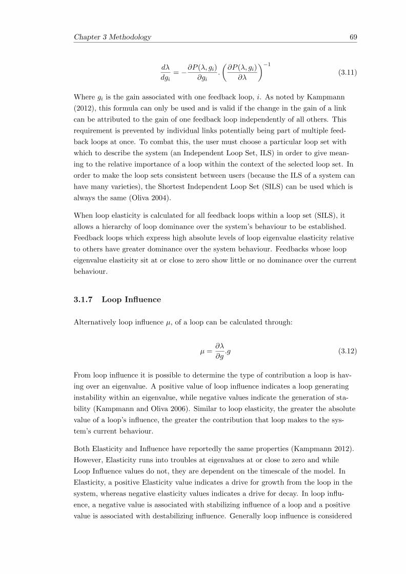
Chapter 3 Methodology 69
dλ
dgi= −∂P (λ, gi)
∂gi.
(∂P (λ, gi)
∂λ
)−1(3.11)
Where gi is the gain associated with one feedback loop, i. As noted by Kampmann
(2012), this formula can only be used and is valid if the change in the gain of a link
can be attributed to the gain of one feedback loop independently of all others. This
requirement is prevented by individual links potentially being part of multiple feed-
back loops at once. To combat this, the user must choose a particular loop set with
which to describe the system (an Independent Loop Set, ILS) in order to give mean-
ing to the relative importance of a loop within the context of the selected loop set. In
order to make the loop sets consistent between users (because the ILS of a system can
have many varieties), the Shortest Independent Loop Set (SILS) can be used which is
always the same (Oliva 2004).
When loop elasticity is calculated for all feedback loops within a loop set (SILS), it
allows a hierarchy of loop dominance over the system’s behaviour to be established.
Feedback loops which express high absolute levels of loop eigenvalue elasticity relative
to others have greater dominance over the system behaviour. Feedbacks whose loop
eigenvalue elasticity sit at or close to zero show little or no dominance over the current
behaviour.
3.1.7 Loop Influence
Alternatively loop influence µ, of a loop can be calculated through:
µ =∂λ
∂g.g (3.12)
From loop influence it is possible to determine the type of contribution a loop is hav-
ing over an eigenvalue. A positive value of loop influence indicates a loop generating
instability within an eigenvalue, while negative values indicate the generation of sta-
bility (Kampmann and Oliva 2006). Similar to loop elasticity, the greater the absolute
value of a loop’s influence, the greater the contribution that loop makes to the sys-
tem’s current behaviour.
Both Elasticity and Influence have reportedly the same properties (Kampmann 2012).
However, Elasticity runs into troubles at eigenvalues at or close to zero and while
Loop Influence values do not, they are dependent on the timescale of the model. In
Elasticity, a positive Elasticity value indicates a drive for growth from the loop in the
system, whereas negative elasticity values indicates a drive for decay. In loop influ-
ence, a negative value is associated with stabilizing influence of a loop and a positive
value is associated with destabilizing influence. Generally loop influence is considered
70 Chapter 3 Methodology
easier to interpret and its time dependency is seen only as a minor drawback (Saleh
et al. 2010). A methodical breakdown of implementing LEEA can be found in Guner-
alp et al. (2005) and Guneralp (2006).
Determining which eigenvalues to focus on:
In EEA (Forrester 1982), in order to determine dominant structures within a model,
the general approach was to select a dominant eigenvalue with which to focus analy-
sis as this inherently would hold the most influential structures of system behaviour
(Guneralp 2006). Eigenvalues are used in an extensive number of fields for a variety
of reasons (i.e. mechanical engineering, physics, image processing, linear systems) and
generally across all fields a dominant eigenvalue from a set is the one which holds the
highest absolute value.
As an example, considering five eigenvalues with the values -10, -4, 0, 2 and 9, the
eigenvalue holding -10 would be dominant. Intuitively this would mean that for loop
dominance analysis the -10 eigenvalue would be prioritised for its influential loop struc-
tures in order to monitor which loops are influencing the behaviour expressed by the
most dominant eigenvalue.
However, in linear systems and particularly in matters of system stability and ex-
ponential growth/decay, this concept of a dominant eigenvalue only works while all
eigenvalues are negative. If any eigenvalue within a linear system holds a positive
value, no matter how small its magnitude, it will eventually dominate the system’s
behaviour (Guneralp 2004; Franklin et al. 1994).
In the context of influential feedback structures, a shift in eigenvalue polarity often
infers a change has occurred to which feedback loop is dominating within that eigen-
value. Changing from a dominant negative feedback to a dominant positive feedback
can lead to a reinforcing or runaway behaviour, which eventually destabilizes the sys-
tem. With regards to system stability, eigenvalues which sit at or close to zero and
eigenvalues which hold large real positive magnitudes can be seen as more important
than eigenvalues with larger negative magnitudes.
The eigenvalue of most interest regarding system stability and therefore the one whose
loop dominance properties should be focused on, is determined by which holds the
highest positive real value at any point in time, even if there are negative eigenvalues
with greater absolute values. If all eigenvalues are negative then the dominant eigen-
value is taken to be the one whose real part holds the largest absolute value. The real
part of the eigenvalue is used to determine eigenvalue dominance regardless of whether
it is a complex number or not. Loop eigenvalue elasticity and loop influence in the
dominant eigenvalue represent the most dominant structural drivers of the system. If
more than one eigenvalue shows high dominance, then behavioural drivers must be
determined from a comparison of loop dynamics across those eigenvalues.

Chapter 3 Methodology 71
3.2 A Worked Example: Forming the Jacobian Matrix
and its connections to Feedback Loops
The following example uses Lokta-Volterra equations to showcase how the first princi-
ples used in LEEA work.
Lokta-Volterra or the predator-prey interactions take the following equations:
dx
dt= αx− βxy (3.13)
and
dy
dt= δxy − γy (3.14)
where dxdt is ho the population od pref x changes over time, dy
dt is how the population
of predators y changes over time, α is the birth rate of prey, β is the rate of preda-
tion of the predators on the prey, δ is the growth rate factor of the predators, with the
growth rate of predators, δxy, reliant on the population of prey and γ is the natural
death rate of predators.
In system dynamic form, these two equations form figure 3.4:
Figure 3.4: The system dynamic form of the predador- prey equations. This dia-gram is an example of how one might find an system dynamic model, with variables
labelled as opposed to their equation equivalents.

72 Chapter 3 Methodology
This next image shows the same diagram with all variables written out for each com-
ponent, and all causal links which are part of feedback loops assigned their link gain
in algebraic form (figure 3.5):
Figure 3.5: The system dynamic form of the predador- prey equations. This dia-gram shows how all of the equations of Lokta-Volterra fit into system dynamic model
form.
Now the Jacobian Matrix for the lokta-volterra equations takes the general form:
J =
∣∣∣∣∣ ∂x∂x
∂x∂y
∂y∂x
∂y∂y
∣∣∣∣∣ . (3.15)
We get:
J =
∣∣∣∣∣ α− βy −βxδy δx− γ
∣∣∣∣∣ . (3.16)
The Jacobian Matrix is a representation of all of the interactions that occur between
the stocks (in this case, between the predators and prey) within the system. Note
that each component of the Jacobian Matrix can be made using the gains of the links
within the system dynamic diagram. The components of the Jacobian Matrix, which
is used to calculate the system’s eigenvalues, is made up of the link gains of the sys-
tem. Intuitively, the gain of a feedback loop of the system can also be calculated as
the product of the links that form their structure.
Thus, the gain of the balancing feedback loop which connects the predator and prey
populations, labelled ‘B’ in the diagram structurally is formed of the link from prey

Chapter 3 Methodology 73
population to predator births which holds the link gain δy and from predator popu-
lation to prey deaths which holds the link gain −βx. So the balancing feedback loop
holds a loop gain of −βδxy.
When a change occurs within the system, it will cause one if not more of the variables
to change in value. This value change gets reflected in the gain of any loop which con-
tained that variable as well as changing the values within the systems Jacobian Matrix
and therefore its eigenvalues. It is because of this that any changes which occur within
the eigenvalues of the system’s eigenvalues can be linked to the changes which are oc-
curring within the feedback loops, and the relative influence of each feedback loop on
the system can be calculated within LEEA.
3.3 Interpretation of Outputs
The following section overviews a series of typical outputs which a user might expect
to gain from conducting LEEA on a system model. The outputs are largely extracts
from the Naumov & Oliva (2017) online support material and software package for
running LEEA. However, to aid understanding of what happens at every step, this
section also provides examples of what outputs look like, which are calculated in the
background of the online software and helps to explain how to interpret them.
Outputs of the system dynamic model, eigenvalues, loop gains, loop eigenvalue elastic-
ities and loop influence values are all output within the online software package (Nau-
mov & Oliva 2017. Their outputs are predominantly graphical, but eigenvalues and
loop gains can also be output in table format, displaying specific values. The eigen-
value and loop gain data series can be used to acquire specific values for each time
step in a system’s model output. These time steps correspond 1 to 1 with the time
steps of the system dynamic model.
Figure 3.6 shows a section of the data series of 21 time steps from the eigenvalue cal-
culation of the LEEA code. The first column shows time steps and the following columns
show the values of each eigenvalue of the system. This particular system had three
stocks and therefore three eigenvalues, so three columns of data were produced. As
eigenvalues can take the form of complex numbers, figure 3.6 shows the values of the
real numbers and figure 3.7 shows the imaginary values across this section. As shown
in figure 3.7, eigenvalues 1 & 2 express imaginary values for 3 timesteps showing that
the system experiences oscillatory dynamics at this point in time.
Each time step of these data series can then be plotted in graphical form, where each
eigenvalue is shown for its real vs. imaginary values. The following plot shows time
step 78 of the above data (Figure 3.8).

74 Chapter 3 Methodology
Figure 3.6: Data series from an eigenvalue calculation (real part) showing 21 timesteps from 60-80. Columns 2-4 represent eigenvalues 1 2 and 3 of the system.
Figure 3.7: Data series from an eigenvalue calculation (imaginary part) showing 21time steps from 60-80. Columns 2-4 represent eigenvalues 1 2 and 3 of the system.
Figure 3.8: Real and Imaginary eigenvalues presented in graphical form. The x axisis the real part and y axis the imaginary part. Eigenvalues are represented with blue
dots. This graphical form shows just one time step in the data series.
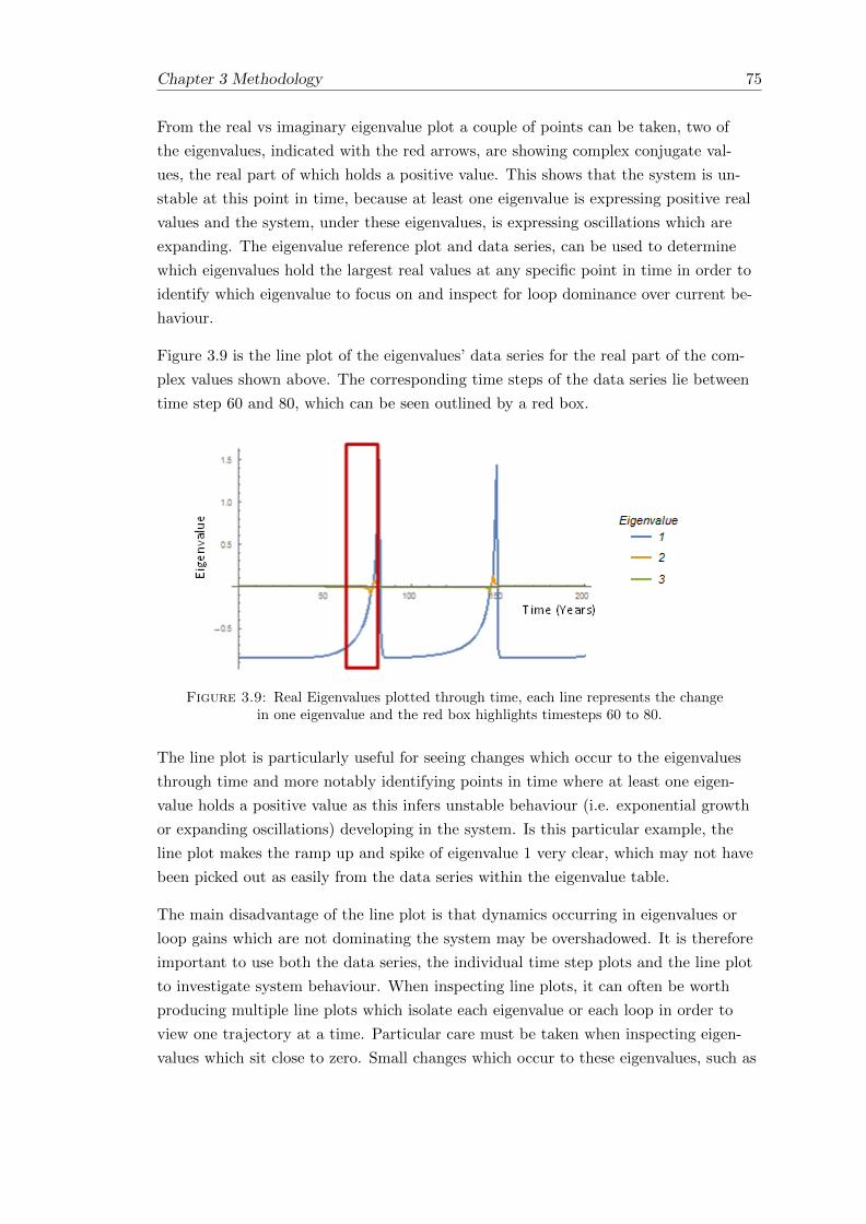
Chapter 3 Methodology 75
From the real vs imaginary eigenvalue plot a couple of points can be taken, two of
the eigenvalues, indicated with the red arrows, are showing complex conjugate val-
ues, the real part of which holds a positive value. This shows that the system is un-
stable at this point in time, because at least one eigenvalue is expressing positive real
values and the system, under these eigenvalues, is expressing oscillations which are
expanding. The eigenvalue reference plot and data series, can be used to determine
which eigenvalues hold the largest real values at any specific point in time in order to
identify which eigenvalue to focus on and inspect for loop dominance over current be-
haviour.
Figure 3.9 is the line plot of the eigenvalues’ data series for the real part of the com-
plex values shown above. The corresponding time steps of the data series lie between
time step 60 and 80, which can be seen outlined by a red box.
Figure 3.9: Real Eigenvalues plotted through time, each line represents the changein one eigenvalue and the red box highlights timesteps 60 to 80.
The line plot is particularly useful for seeing changes which occur to the eigenvalues
through time and more notably identifying points in time where at least one eigen-
value holds a positive value as this infers unstable behaviour (i.e. exponential growth
or expanding oscillations) developing in the system. Is this particular example, the
line plot makes the ramp up and spike of eigenvalue 1 very clear, which may not have
been picked out as easily from the data series within the eigenvalue table.
The main disadvantage of the line plot is that dynamics occurring in eigenvalues or
loop gains which are not dominating the system may be overshadowed. It is therefore
important to use both the data series, the individual time step plots and the line plot
to investigate system behaviour. When inspecting line plots, it can often be worth
producing multiple line plots which isolate each eigenvalue or each loop in order to
view one trajectory at a time. Particular care must be taken when inspecting eigen-
values which sit close to zero. Small changes which occur to these eigenvalues, such as
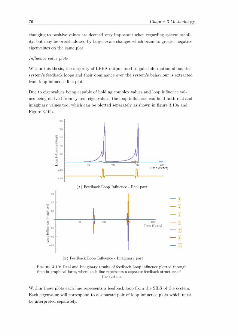
76 Chapter 3 Methodology
changing to positive values are deemed very important when regarding system stabil-
ity, but may be overshadowed by larger scale changes which occur to greater negative
eigenvalues on the same plot.
Influence value plots
Within this thesis, the majority of LEEA output used to gain information about the
system’s feedback loops and their dominance over the system’s behaviour is extracted
from loop influence line plots.
Due to eigenvalues being capable of holding complex values and loop influence val-
ues being derived from system eigenvalues, the loop influences can hold both real and
imaginary values too, which can be plotted separately as shown in figure 3.10a and
Figure 3.10b.
(a) Feedback Loop Influence - Real part
(b) Feedback Loop Influence - Imaginary part
Figure 3.10: Real and Imaginary results of feedback Loop influence plotted throughtime in graphical form, where each line represents a separate feedback structure of
the system.
Within these plots each line represents a feedback loop from the SILS of the system.
Each eigenvalue will correspond to a separate pair of loop influence plots which must
be interpreted separately.

Chapter 3 Methodology 77
From these plots, the lines which hold the highest values correspond to the feedback
loops which hold the highest influence over the eigenvalue and these are often the
feedback loops which are paid most attention when concerned with the leading causes
of system behaviour. As noted from the Eigenvalue Line plot (figure 3.9), the dynam-
ics occurring in some of the loop influence values can be overshadowed by feedback
loops expressing much higher values. To compensate for this, the graphs can either
be plotted with logarithmic scales, the feedback influence values can be plotted sepa-
rately, or the plot range can be altered as shown in figure 3.11.
Figure 3.11: Feedback loop influence showing subsection of the real part with aspecified shorter range for closer interpretation of results.
To identify the most influential loop structures in comparison to one another, absolute
values may also be plotted, figure 3.12.
Figure 3.12: Feedback loop influence showing absolute values.
In figure 3.12 we see feedback loop 2, (orange line) dominating the system with all
other loops sitting at or close to zero, appart from two spikes of feedback loop 5 (pur-
ple line) which can be seen building influence exponentially over time until it over-
takes the influence of loop 2, only to quickly settle back down to zero.

78 Chapter 3 Methodology
If an individual time step for loop influences needs to be isolated, a graphical output
similar to that available for the Eigenvalue data can be plotted, as shown in Figure
3.13.
(a)
(b)
Figure 3.13: A) Feedback loop influence values of seven loop structures for a singlepoint in time of a simulation. The values are displayed as absolute values and their
real part. B) Feedback loop influence values plotted in graphical form
Figure 3.13 shows time step 78, chosen here to show the loop influence output at the
same time step as that chosen for the eigenvalue plot in figure 3.9. In the loop influ-
ence time step plots, each dot represents a feedback loop within the system. Unlike
the eigenvalue plot, the y axis now represents the real part of the complex pair and
the x axis represents the absolute values of the real and imaginary parts combined.
The main purpose of this plot is to easily identify the order of hierarchy which the
loops hold over the system at that point in time.
3.4 Regarding Error in LEEA
In order to make use of the Jacobian Matrix and its Eigenvalues, LEEA requires the
system to be linearized at each point in time. LEEA therefore treats each time step
as an isolated point in time and any points between the chosen time steps when eigen-
values or loop influence plots are plotted through time are subject to error because
the plotting process simply assumes a linear trend between points. The extent of this
error will depend on the model being analysed and the time step in question. The
more complex the model’s dynamics, the more frequent the models dynamics, and the
larger the time step between points calculated by LEEA, the more likely the output of

Chapter 3 Methodology 79
LEEA is to be misinterpreted. There are two simple solutions to reduce this potential
misinterpretation:
1. Reduce the time steps within the model simulation at which LEEA is calculated
(i.e. from 1 to 0.125).
2. At times where there are lots of dynamics occurring within the systems output
only refer to LEEAs outputs at individual time steps, prioritising individual time
plots, over plots which hold the entire time series.
3.5 When to use and when not to use LEEA
When deciding whether or not to use LEEA on a prebuilt model system, there are
a few properties of the models structure which the analyst should look for. Here is
a quick guide to provide a model user with a rough idea as to whether LEEA is an
appropriate analysis for a model. This guide assumes that the user has a system dy-
namic model in front of them and will help to determine LEEAs applicability from
structural properties of the model alone.
1. Proportion of the model included within feedback structures (Are all the stocks
connected through feedback loops?)
LEEA is optimised when all stocks are connected in some way through feedback
loops. The more stocks that are connected in this way, the more LEEA will be
able to analyse behaviours occurring across the entire system. While this will
not always be the case as many systems, particularly in socio-ecology, are key
topics of research and not functioning as intended due to lack of feedback be-
tween key areas.
2. Number of stocks (user should be wary if stock no. is >13)
One of the limitations of LEEA discussed within this thesis is the vast amounts
of data that LEEA produces which is not needed to determine key drivers of
the system. The number of eigenvalues needed to be interpreted within a sys-
tem increases at a 1:1 ratio with the number of stocks. As the stock number
increases, data output increases and interpretation takes more time. Currently
the largest model where LEEA was still comfortably interpreted and had utility
held 13 stocks (Oliva 2016). While LEEA will still comfortably analyse anything
with >13 stocks, it is up to the user how much time and effort they are willing
to spend interpreting all the data.
3. Number of loops (the greater the ratio of loop no. to stock no. the better, within
reason)

80 Chapter 3 Methodology
The number of feedback loops within a system can vary dramatically for a rel-
atively small number of stocks, purely based on the number of interactions held
between them. There is no general rule for the number of feedback loops a user
of LEEA should look for in a model. However, generally speaking, the more
feedback loops there are compared to the number of stocks, the more use an an-
alyst will get out of LEEA, while the closer the ratio of loops to stock number
is to 1:1, the less information LEEA will provide. The benefit of having a high
ratio of feedback loops to stock no. will, of course, have an upper limit, where a
model with too many feedback loops compared to its stock number may be in-
appropriate for the task it was intended for. The user is advised to use common
sense and good modelling practice when considering LEEA, whereby often the
best model is the simplest one.
If there were to be a ‘sweet spot’ for models where LEEA would have the most util-
ity it would be on models with up to 13 stocks (as shown so far by Oliva (2016)),
where the loop to stock ratio sits somewhere between 2:1 and 3:1 (of the ratios ex-
plored within this thesis) and where each stock of the system is connected to at least
one other stock by a minimum of one feedback loop.
As models get larger, the best approach is initially to determine which data LEEA
produces is going to be appropriate for the questions being asked. This can be achieved
by taking the time to carefully inspect the eigenvalue and loop influence plots of the
system, breaking it down into sections if necessary and producing new plots where the
dynamics become complex.
3.6 Regarding LEEA’s ability to analyse system’s struc-
ture inside vs. outside a loop.
In LEEA’s analysis of a system, it is only able to account for structures that are in-
herently part of feedback loop structures. While LEEA successfully identifies which
feedback loops are driving system behaviour, it does not directly identify which parts
of a system are driving and/or kick starting those dominant loops.
The example in figure 3.14 shows a simplified version of processes involved in lake eu-
trophication. This structure would be part of a larger model, with many more feed-
back processes. The important thing to note structurally is that there is a long causal
chain (multiple causal links connected together) leading up to what can be assumed to
be one of the lake system’s most dominant feedback loops. Here, LEEA would pick up
on the dominant reinforcing feedback loop on the system (labelled R), giving rise to
the conclusion that this loop is driving system behaviour and must become the focus
of an operation if the behaviour of this system is to be changed. However, LEEA is

Chapter 3 Methodology 81
not able to account for the causal chain leading into this feedback loop, because it it-
self is not part of a feedback structure. There is a long line of events and system com-
ponents represented here by letters a to f, which feed into the loop’s structure. In this
particular example, we know that crop fertilizer has a large influence on and would
be a likely leverage point for this system taking into account practical and economic
viability.
Figure 3.14: Example of a chain and loop structure connected to form part ofa larger model structure. Letters a to f represent non specified auxillary variables
within a causal chain leading into the feedback structure.
The point is that it is important to use the information gained from LEEA as a means
to further explore and understand the system and not just take the most dominant
loop structures as the be all and end all of system control and manipulation. When
we are considering system leverage points, the best way to influence a dominant loop
structure might not lie within the loop itself, but within the system components and
causal links leading into that loop.

82 Chapter 3 Methodology
Chapter 4: Chapter Preface
Chapter 4 initiates a series of case studies used to examine and access Loop Eigen-
value Elasticity Analysis (LEEA). The assessments primarily focus on feedback loop
dominance within complex ecological and socio-ecological systems, investigating LEEA’s
ability to provide novel information surrounding model structure and system behaviour
that cannot be gained from model conception or output alone. Each chapter from 4
to 7 represents a separate case study, with chapters 4-6 primarily based on dynamics
found within lake ecology and chapter 7 based on coral reef ecology. Chapters 4, 6 and
7 are capable of acting as stand-alone case studies, each of which investigates LEEA
in a separate context, with chapter 5 acting as an extension to the findings of chapter
4. Collectively the chapters act as an assessment of LEEA’s application, novelty and
utility, extending and reinforcing the knowledge gained in each previous chapter.
Chapter 4 begins with LEEA’s application to a small system dynamic model based
around a shallow lake system which undergoes eutrophication. It has previously been
expressed and shown by the developers of LEEA that the technique excels at analysing
collapsing or regime shifting behaviour within systems. In Chapter 4, a small eutrophic
lake model is chosen to explore the capabilities of LEEA in order to show how it per-
forms at analysing dynamic behaviours that are well known within the field of lake
ecology. While LEEA’s ability to analyse different dynamic behaviours is well estab-
lished within the literature, it is the context of its application to complex ecological
and socio-ecological models and the implications that the success of the technique
could have for system understanding, modelling practices and policy design that makes
this application of LEEA so important.

Chapter 4
Structural Loop Analysis of
Complex Ecological Systems
4.1 Abstract
Ecosystems are complex systems that can be challenging to understand. We urgently
need to assess human impacts on ecosystems which cause changes in structural feed-
backs producing large, hard to reverse changes in state and functioning. System dy-
namics has proven to be a useful and versatile methodology for modelling complex
systems given the comparative ease with which feedback loops can be modelled. How-
ever, a common issue arises when models become too large and structurally complex
to understand the causal drivers of system behaviour. There is a need for an interme-
diate level of analysis capable of identifying causal driving structures and dynamics,
regardless of model complexity. This study investigates Loop Eigenvalue Elasticity
Analysis, a structural analysis technique commonly used in business and economic sys-
tem dynamics models, and evaluates its utility for identifying feedback loop structures
responsible for behavioural changes in complex ecological systems. The approach is
demonstrated by analysing a simple lake system model that has been extensively stud-
ied in the past for its capacity to undertake critical transitions between alternative
stable states. We show how the dominance of feedback loops can be tracked through
time building influence over the system’s behaviour decades prior to the actual col-
lapse in the system. We discuss our findings in the context of the study of complex
ecosystems, and socio-ecological systems.
Keywords: Complexity, Ecosystem, Socio-Ecology, Structural Analysis, Feedback
Loop, Critical Transition, Modelling.
83

84 Chapter 4 Structural Loop Analysis of Complex Ecological Systems
4.2 Introduction
Socio-ecological system models represent the interconnected nature of society and the
environment. These systems are complex, able to exhibit emergence and self-organisation,
with behaviours arising endogenously through non-linear dynamics (Guneralp 2006).
A defining characteristic of socio-ecological systems is multiple feedback loops which
collectively form the internal structure of the system (Meadows 2008), but disentan-
gling and prioritising those feedbacks in order to understand system behaviour and
develop effective policy is no simple task. Indeed, a necessary condition for labelling
a system a socio-ecological system is that of a feedback loop operating between social
and ecological elements. It is such feedback loops that are often the primary drivers
of emergent system behaviour (Sterman 2001). Here use of the term ‘driver’, in the
context of structural feedback loops, means the main endogenous cause of a system’s
behaviour. Systems may exhibit strong non-linear dynamics which are explored with
the concepts of critical transitions between alternative stable states, regime shifts,
and tipping points with potentially hard or effectively impossible to reverse changes
in state due to properties of hysteresis (Scheffer 2009; Carpenter 2005). Consequently
socio-ecological systems are hard to understand, hard to predict and difficult to man-
age (Meadows 2008). Maintaining socio-ecological systems in desirable states and un-
derstanding why their behaviours change through time is fundamental for economic
growth, poverty alleviation and general wellbeing (United Nations 2015 2015; Scheffer
2009).
Process based, mechanistic, bottom up modelling has been used to understand socio-
ecological systems (Verburg et al. 2016). System dynamics is one methodology that
can be used to increase our understanding of such systems. System dynamics models
are structural representations of dynamic real world systems. They take a resource
based view of the world, characterising a system through a set of stocks and flows in
order to represent its structure. Stocks are often, but not only, material goods, and
flows are pathways of material between stocks (Ford 2010).
System dynamics has an established track record of being applied to ecological and
socio-ecological modelling (e.g. Ford 2010; Meadows 2008; Dyson and Chang 2005;
Saysel et al. 2002; Vezjak et al. 1998). Powerful and intuitive software packages such
as Vensim (Ventana Systems Inc. 2006) and STELLA (isee systems 2016) and the ex-
change of established models and modelling libraries allows potentially very complex
systems to be represented with models that produce output via computationally effi-
cient numerical integration schemes. Whilst this has allowed a wide range of system
dynamic models to be developed, it has, at times, produced models that are difficult
to assess with regards to their overall utility in increasing our understanding of the
real world systems. Such models can be challenging to parameterise, validate and in-
terpret (Voinov and Shugart 2013). The risk is that some system dynamics models are

Chapter 4 Structural Loop Analysis of Complex Ecological Systems 85
essentially black box representations of the target system making them effectively as
hard to interpret (Voinov and Shugart 2013).
In this study, we investigate a methodology that could increase our understanding,
and potentially prediction, of large changes in system structure and functioning through
a quantitative analysis of feedback loops as endogenous drivers of system behaviour.
Rather than searching system-level properties and variables for statistical properties of
impending critical transitions (Scheffer 2009; Scheffer and Carpenter 2003), we instead
focus on the structural properties of the system which drives such behaviour.
We are motivated to understand how these sub-processes function collectively in pro-
ducing system behaviour. One analogy is that if the system dynamics model is an or-
ganism that we can observe via its output, then we seek to understand the processes
that drive such behaviour by peering within the model in order to identify ‘organs’
and ‘physiological processes’. This analysis can be used in conjunction with evaluation
of the system output, its stability, and identification of the most important individual
components with respect to specific behaviours. In this study we investigate the mech-
anisms responsible for generating stability and instability within a system, how these
change through time, whether stability or instability is dominated by an individual
driver or generated by several, and how these drivers change in dominance as a system
undergoes a phase shift, or transitions between stable and unstable states.
The technique explored within this study is known as Loop Eigenvalue Elasticity Anal-
ysis (LEEA). LEEA expands on the knowledge gained from linear stability analy-
sis and graph theory, identifying a set of feedback loops within a system’s structure
known as the Shortest Independent Loop Set or SILS (Oliva 2015; Oliva 2004), which
are collectively responsible for generating stability and instability within the system.
A description of SILS, what it does and why it is necessary can be found within the
Supplementary Information section 1 of this paper, under ‘Loop Eigenvalue Elastic-
ity’. LEEA then structurally analyses the loop set, identifying which feedback loops
are dominating the system’s behaviour at any point in time, generating a hierarchy of
the influential feedback loops of the system.
Exploring ecosystem dynamics through the study of feedback loops has already shown
potential to improve our mechanistic understanding of critical transitions and stabil-
ity within lake systems (Kuiper et al. 2015). While the methodology of Kuiper et al.
(2015) focusses primarily on food webs, their motivations of finding feedback loops
within a lake ecosystem in order to determine stability and critical transitions between
two regimes is similar to this study.
Previous research has demonstrated that LEEA can increase understanding of system
behaviour and causal drivers across a range of model systems (Oliva 2015; Kampmann
2012; Goncalves 2009; Kampmann and Oliva 2008; Guneralp 2006; Guneralp et al.
2005). Thus far the method has only seen limited use in the field of socio-ecology in

86 Chapter 4 Structural Loop Analysis of Complex Ecological Systems
the context of agriculture (Bueno 2013; Bueno 2012) and the Baltic cod fishery as a
potential practice to be undertaken after conducting generalized modelling (Lade and
Niiranen 2017). Here we extend this work and evaluate LEEA in the context of crit-
ical transitions and regime shifts, implementing loop analysis of a small lake model
which can undergo critical transitions between clear and turbid states as a conse-
quence of human drivers.
A full explanation of the limitations of the LEEA technique, along with many solu-
tions to these limitations have been addressed by Guneralp (2006). Efforts to make
the technique more automated have been conducted by Sergey Naumov and Rogelio
Oliva and can be found online (Naumov & Oliva 2017).
The model
The model chosen to demonstrate the application of LEEA has been developed from
Carpenter (2005) which formulated a simple model of a shallow lake, Lake Mendota
in Wisconsin, USA, using empirical data for soil, lake and sediment phosphorus levels.
The model was bistable as increasing phosphorus input in the lake produced a critical
transition with a sudden shift from a clear to a turbid state. Shallow lakes are classic
examples of bistable systems, capable of discrete transitions from clear to eutrophic
conditions (Wang et al. 2012) and their properties are relatively well known (Carpen-
ter et al. 2011; Carpenter 2005; Scheffer 2004; Ludwig et al. 2003; Scheffer and Car-
penter 2003) with current theories attributing many eutrophic tipping events to large
influxes of phosphorus through anthropogenic activity such as fertiliser runoff from
farms in the lake catchment area. The model has been chosen for two principle rea-
sons: 1) The main focus of the model’s dynamic behaviour is a regime shift, allowing
for an investigation of feedback loop behaviour around the point of a critical transi-
tion. 2) The model is relatively simple, allowing for a quantitative account of LEEA
to be presented, and assessment of LEEA’s utility for the analysis of such systems.
4.3 Background
Lake Eutrophication
Lake Mendota is a shallow freshwater lake surrounded by agricultural fields which re-
ceive ample supplies of phosphorus fertiliser. Soil erosion leads to excess phosphorus
from the fertiliser, not taken up by vegetation, to be washed into surrounding streams
and rivers, eventually leading to the lake. This process concentrates phosphorus runoff
from the lake’s catchment area into lake water where the excess of nutrients causes al-
gal blooms to form. The formation of these blooms leads to plant death by blocking
sunlight, fish death through generating anoxic conditions and phosphorus recycling
from the lake sediment, which reinforces the high levels of phosphorus in the system

Chapter 4 Structural Loop Analysis of Complex Ecological Systems 87
(Scheffer 2009; Scheffer 2004; Scheffer and Carpenter 2003). Combined, these events
can cause a lake to undergo a critical transition from a nutrient poor, high biodiver-
sity, clear water state to a nutrient rich, low biodiversity, eutrophic state.
Lake eutrophication is not only detrimental for the lake biota and biodiversity, it can
have adverse effects on the system’s provision of ecosystem services. Provisioning ser-
vices are impacted primarily through the collapse of fisheries. Cultural services such
as recreation and tourism can be affected (Dodds et al. 2008; Scheffer 2009). Attempts
to return a eutrophic lake to its previous clear conditions require the levels of phos-
phorus in the lake to be reduced but these systems can have large hysteresis loops,
making them challenging to recover (Carpenter et al. 1999b). If nutrient levels are re-
duced sufficiently, the lake becomes capable of undergoing a reverse critical transition,
returning to its former low nutrient, clear state, however such a reverse in conditions
may take many years (McCrackin et al. 2017; Wang et al. 2012).
Feedback Loops
Feedback loops can emerge in systems as coincidental structures when multiple in-
teractions form between components that link an output back to its original source.
Feedback loops are capable of existing in one of two forms, positive or negative. Posi-
tive feedback loops are known for generating reinforcing behaviour in a system and are
associated with exponential growth or collapse, and are often found to be the causes
of system instability. Negative feedback loops generate balancing behaviour within a
system; they are associated with oscillatory trends or dampening and are often found
to be the cause of system stability (Ford 2010). While the premise of positive and neg-
ative feedback can be easily understood, it is the interconnected nature of multiple
feedback structures together that makes the behaviour they generate difficult to pre-
dict.
Feedback loops can be represented in models by constructing connections between
any two system variables that interact with each other, where multiple connections
join together to form a loop. These can be represented as coupled ordinary equations.
Here we focus on the structural properties of the model system and the feedback loops
which drive their behaviour. In 1982, Forrester (1982) first used concepts established
within classical control theory, using eigenvalues to describe the behaviour of linear
systems, to decompose the behaviour of linearized system dynamic models into simple
reference modes. Forrester (1983) & Forrester (1982) then used this method to de-
velop the concept of eigenvalue elasticity to model parameters which became known
as Eigenvalue Elasticity Analysis (EEA). Loop Eigenvalue Elasticity Analysis (LEEA)
was introduced in 1996, by Kampmann (2012) who extended the work of EEA, for-
mally linking the strength of individual feedback loop structures to system eigenval-
ues. LEEA has since been applied to economic and industry modelling, with method-
ological refinements being made over this period (Saleh et al. 2010; Guneralp 2006;

88 Chapter 4 Structural Loop Analysis of Complex Ecological Systems
Kampmann and Oliva 2006). LEEA is based on the ability to describe a system’s be-
haviour through a set of eigenvalues at any moment of time and relate changes in out-
put to influential feedback loop structures within the system.
The strength and sometimes even sign of feedback loops can alter in response to exter-
nal driving. Changes which occur to a system can generate changes to the strengths
(i.e. the change in output from a change in input) of individual links (the structural
connection held between two system variables). Changes to the strength of individual
links consequently change the strength of feedback loops, which as a result are able to
generate changes to the system’s eigenvalues. The ‘strength’ of a link may be referred
to as the link gain and likewise the ‘strength’ of a feedback loop may be referred to
as the loop gain, further explained in the methodology section (see below) (Guneralp
2006). Changes in feedback loop gain which create large changes to eigenvalues indi-
cate high influence of that feedback loop on the current behaviour, while changes in
loop gain which produce small changes to eigenvalues indicate little to no influence of
that feedback loop on the current behaviour. LEEA is therefore able to identify how
much an individual feedback loop has dominance over the current system behaviour,
allowing the user to identify a hierarchy of loop influence.
4.4 Methodology
The following section gives a high level overview of the steps required to undertake
LEEA. The formalism and expansions on the following steps can be found in the Sup-
plementary Information section 1.
Calculation of loop eigenvalues and loop influence values is conducted via the follow-
ing process:
1. The Jacobian Matrix of the linearized dynamical system model
2. Eigenvalues of the Jacobian matrix
3. Loop Gain
4. Loop Elasticity & Loop Influence
1. The Jacobian Matrix is an nxn square matrix where each element of the matrix
is a partial differential equation that represents how one stock affects another
stock’s derivative, when all other stocks are kept constant. The matrix therefore
represents the links that exist between stocks (Goncalves 2009).

Chapter 4 Structural Loop Analysis of Complex Ecological Systems 89
2. Eigenvalues are calculated from a system’s Jacobian matrix and therefore the
number of eigenvalues of a system is equal to the number of stocks in that sys-
tem. From linear stability theory, eigenvalues can be used to determine if a sys-
tem at a fixed point is stable or unstable (Glendinning 1994). Eigenvalues are
capable of being real, or complex numbers with a real and imaginary part. An
eigenvalue with a real, negative value is associated with the system converg-
ing towards a fixed point. If the real part of all eigenvalues are negative, then
the fixed point is stable. An eigenvalue with a real, positive value is associated
with the system diverging away from a fixed point. Therefore, if the real parts
of any of the eigenvalues are positive, then the fixed point is unstable. Eigenval-
ues which are complex are associated with oscillatory behaviour and mean the
system will express either sustained oscillations, expanding oscillations or damp-
ening oscillations if the real part of the complex eigenvalue is zero, positive or
negative respectively.
Eigenvalues which sit at or close to zero play a vital role in determining the sys-
tem’s state of stability. A system is determined to be unstable for any given
time period while at least one eigenvalue holds a real positive value. This means
that large changes in negative eigenvalues which remain negative, portray less
information about a system’s state of stability than small changes which happen
to eigenvalues at or around zero.
When interpreting output from LEEA, it is possible to gain a different hierarchy
of loop dominance from each eigenvalue within a system as different elements
will be responsible for generating each eigenvalue (Oliva 2016). This can lead to
multiple outputs with apparent contrasting results as different feedback loops
are capable of expressing dominance across different eigenvalues. To reduce con-
fusion, eigenvalues holding the largest real positive values may be prioritised first
for interpretation. The greater value of an eigenvalue, the more it determines the
system’s current behaviour. While this allows the elasticity and influence plots
of some eigenvalues to be prioritised and others largely ignored, attention must
be paid to eigenvalues switching dominance and to eigenvalues at or close to zero
as this would change which eigenvalues must be prioritised.
3. Loop Gain reflects the overall strength of a feedback loop and is the product of
the link gains whose associated links join together to form a loop. Link gains
reflect the strength of influence of one variable upon another. An increase in an
output with a fixed input infers an increase of gain within that link. Loop Gain
is required to compare changes within the system’s feedback loops against the
system’s eigenvalues.
4. Loop Elasticity is the change in eigenvalue relative to change in loop gain (Kamp-
mann and Oliva 2008; Kampmann and Oliva 2006). Thus loop elasticity indi-
cates how much a loop contributes to changes within an eigenvalue. Loops with
90 Chapter 4 Structural Loop Analysis of Complex Ecological Systems
high absolute values of elasticity contribute the most to changes within an eigen-
value.
Loop Elasticity derives from an inherent connection that exists between system
eigenvalues and loop gain through a system’s characteristic polynomial (P (λ))
(Kampmann 2012). A characteristic polynomial takes the form P (λ) = |λI − J |,where I is an Identity Matrix and J, the system’s Jacobian Matrix. Loop gains
make up the coefficients of the characteristic polynomial, while eigenvalues are
determined as its roots. This connection between the two means that changes
which occur in the gain of a loop can have a direct impact on the system’s eigen-
values and the extent of this impact can be measured in the form of Loop Elas-
ticity.
Loop Influence values determine the type of contribution a loop is having over
an eigenvalue. A positive value of loop influence indicates a loop generating in-
stability within an eigenvalue, while negative values indicate the generation of
stability (Kampmann and Oliva 2006). Similar to loop elasticity, the greater the
absolute value of a loop’s influence, the greater the contribution that loop makes
to the system’s current behaviour.
4.5 Results
The PLUM model
Carpenter’s study of Lake Mendota (Carpenter 2005) is represented using system dy-
namic terms in the form of the PLUM model ((P)Phosphorus (L)Loops in (U)Soil and
(M)Sediment) (Figure 4.1).
System dynamic modelling is carried out using Vensim, which effectively numerically
integrates Carpenter’s series of ordinary differential equations. The model allows the
user to visualise the number, polarity, position and interaction of the system’s feed-
back loops alongside providing the ability to easily implement and manipulate the sys-
tem’s structure and dynamics. While representing the system’s internal structure in
this manner is not necessary for LEEA as it can be computed purely numerically; it
is easy to do the computation in a software such as Vensim, so it is worth the effort
of building a system dynamic model. Vensim is not necessary for this analysis, but
it allows for easy manipulation of loop structures and numerical solutions, which fa-
cilitates model construction. Vensim also compliments the online materials Naumov
& Oliva (2017), which have been designed to streamline the analysis process, includ-
ing the ability to extract time series data from each simulation quickly and effectively.
The packages used to calculate the results within this article were from the 2017 on-
line material and require Vensim and Mathematica to reproduce, a link to the PLUM

Chapter 4 Structural Loop Analysis of Complex Ecological Systems 91
model and Mathematica codes used to generate the results can be found in the Sup-
plementary Information, section 2.
The Carpenter (2005) study describes dynamic properties of phosphorus levels within
a lake system as a set of coupled differential equations. This simple model, which
is typically parameterised to empirical data, relates changes in the concentration of
phosphorus in the water as phosphorus input into the lake increases over time. These
equations model changes of phosphorus within the soil of the land (U), the water of
the lake (P) and the lake sediment (M). A table listing all terms, units and descrip-
tions is given in Table 4.1. The change of soil phosphorus over time if defined thus:
dU
dt= W + F −H − cU (4.1)
with the runoff parameter c being important in driving the dynamics of concentrations
of phosphorus in the water:
dP
dt= cU − (s+ h)P + rM
P q
mq + P q(4.2)
Phosphorus can be stored or released in the lake sediment thus:
dM
dt= sP − bM − rM P q
mq + P q(4.3)
Derivation of these values can be found in Carpenter (2005). The equations them-
selves have been developed from previous studies of lake dynamics (Carpenter et al.
2003; Ludwig et al. 2003; Carpenter et al. 1999b).
Phosphorus recycling involves stored phosphorus, which has been accumulating in
the lake sediment over year to decadal timescales, being released back into lake wa-
ter as a consequence of chemical reactions driven by anoxic conditions at the bottom
of the lake. The anoxic conditions are generated by populations of bacteria, which
deplete oxygen during their decomposing of organic matter. The increase in organic
matter, and so bacterial decomposition and bottom water anoxia, is a consequence of
increased populations of algae and other lake biota taking advantage of the increasing
levels of phosphorus in the lake water (Scheffer 2009; Carpenter 2005; Scheffer 2004;
Ludwig et al. 2003). The sigmoidal function, the last term of equation 4.2 and 4.3 rep-
resents high levels of phosphorus being reintroduced to the system from the sediment
through phosphorus recycling, as phosphorus levels in the water column become en-
riched from agricultural and non-agricultural sources.
Numerical solutions for the model were computed for 1000 years to recreate Scenario 1
from Carpenter’s model (Carpenter 2005). Scenario 1 undergoes the following changes:

92 Chapter 4 Structural Loop Analysis of Complex Ecological Systems
Symbol Definition Units NominalValue
b Permanent burial rate of sediment P y−1 0.001c P runoff coefficient y−1 0.00115F Annual agricultural import of P to the
watershed per unit lake areag.m−2.y−1 31.6
h Outflow rate of P y−1 0.15H Annual export of P from the watershed
in farm products, per unit lake areag.m−2.y−1
m P density in the lake when recycling is0.5 r
g.m−2 2.4
r Maximum recycling rate of P g.m−2.y−1 0.019q Parameter for steepness of f(P) near m Unitless 8s Sedimentation rate of P g.m−2.y−1 0.7W Nonagricultural inputs of P to the water-
shed prior to disturbance, per unit lakearea
g.m−2.y−1 0.147
WD Nonagricultural inputs of P to the wa-tershed after disturbance, per unit lakearea
g.m−2.y−1 1.55
Table 4.1: Modified from Carpenter (2005). Model parameters, nominal values andunits used to implement PLUM.
0-100 years presettlement conditions, F = H = 0 and W is set toundisturbed conditions.
100-200 years advent of agriculture, W changes to its disturbedvalue (WD).
200-250 years intensive industrialized agriculture, F > H, valuesshown in table 1.
250-1000 years management to balance phosphorus budget of agri-culture, F = H and W maintained at WD.
Table 4.2: Modified from Carpenter (2005). Changes to phosphorus input levelswithin the PLUM model for the first scenario, 0 to 1000 years.
The system has a single steady state value of lake phosphorus concentrations provid-
ing that non-agricultural inputs lie between W and WD and agricultural inputs do not
exceed the annual export of phosphorus through farming products (F = H). Beyond
this regime, the system becomes bistable, having two stable equilibrium between an
unstable equilibrium, with a single steady state value of much higher lake water phos-
phorus concentrations being found when F is 1.7 times greater than H. Analytical
solutions and graphical representation of the system’s bistability can be found in Car-
penter (2005).
Assuming a constant input of additional phosphorus over time, the lake system under-
goes a critical transition at 450 years. Critical transition theory and resilience research

Chapter 4 Structural Loop Analysis of Complex Ecological Systems 93
often associate a change in system states with a shift in dominant feedback loops,
where positive feedbacks drive a system into an alternative state through reinforcing
behaviour, but due to the often complex dynamics involved, little has been done to
actively show this happening (Scheffer 2009; Scheffer and Carpenter 2003). The mech-
anism driving the critical transition within this system is phosphorus recycling, which
reinforces the amount of phosphorus within the lake water and is capable of causing
large influxes of phosphorus to enter the water column long after attempts to control
phosphorus input through the soil have been in place (Scheffer 2009).
Carpenter (2005) provides analytical solutions showing that the system is bistable,
caused as a consequence of phosphorus recycling from the sediment. It is within its
bistable state that the lake is capable of transitioning from its clear-water to turbid-
water attractors following a perturbation. The bistable state also allows for a reverse
transition from turbid-water to clear-water conditions to be possible but this recov-
ery is slowed by the steady release of phosphorus from the lake’s sediments. Carpen-
ter notes that in order to induce a transition back to a clear-water attractor, either
a stochastic event or deliberate management of phosphorus sediment recycling would
have to take place.
A reverse transition was achieved within the model system by maintaining F = H and
converting W back to its undisturbed conditions at 1000 years. Overall, this reduces
the amount of phosphorus entering the lake water, creating a net output of phospho-
rus from the system over time. The reductions in phosphorus within the lake water
undergo a linear decrease through time. However, a critical transition back to a clear
water state does not occur until much later, around year 2050, when phosphorus levels
have reduced well below levels of the original forward tip. The disparity between the
point at which the forward and reverse critical transition occurs is known as hystere-
sis. In shallow lakes the hysteresis effect is often a result of different levels of nutrient
loading (Scheffer 2009) i.e. how much phosphorus is able to enter the system within a
given period of time. Results of the reverse critical transition are shown in figure 4.1
c. LEEA was then used to investigate which loop structures were generating stability
and instability prior to, at and post these critical transitions
The model’s three stocks U, P and M, shown as black boxes within figure 4.1a, relate
to differential equations 1, 2 and 3 of the system. Each stock has an inflow and out-
flow (i.e. Uinput or Uoutput) shown by black double lined arrows which determine
the level of material within the stock, which in this case is phosphorus density. Cloud
shapes within the figure represent sources and sinks of the phosphorus, the specific
locations of which are determined to be outside the scope of the model. Finally, blue
arrows represent the interactions held between all model components which link to-
gether to form the feedback loops that occur between stocks. The model holds a total
of seven feedback loop structures, six of which have been identified by the Shortest In-
dependent Loop Set (SILS) and are labelled in figure 4.1a. The seventh loop is formed

94 Chapter 4 Structural Loop Analysis of Complex Ecological Systems
Figure 4.1: a. The PLUM model a structural representation of Carpenter’s phos-phorus equations (Carpenter 2005) containing the stocks (black boxes) water phos-phorus density (P), soil phosphorus density (U) and sediment phosphorus density(M). The figure also contains system flows (black double arrows) going into and outof each stock, sources and sinks (cloud shapes) and component interactions (bluearrows). . The recreation of Scenario 1 can be seen in figure b. The extension to theCarpenter simulation, to invoke a reverse critical transition in the system can be seen
in c.
from loops 4 and 5 connecting together. The seventh loop is not included within the
SILS as its structure is fully accounted for within the loop set when loops 4 and 5 are
calculated. A breakdown of the components within each of the SILS loops can be seen
in table 4.3.
LoopNo.
Structure Feedback Type
1 M → Moutput → M Negative2 P → Poutput → P Negative3 U → Uoutput → U Negative4 M → phosequ → Moutput − > M Negative5 P → phosequ → Pinput Positive6 M → phosequ → Pinput → P → Minput
→ MPositive
Table 4.3: Loop numbers, structures and loop type within the PLUM model.

Chapter 4 Structural Loop Analysis of Complex Ecological Systems 95
Eigenvalues, loop gains and loop influences were calculated once per year. For the for-
ward critical transition, LEEA was calculated from the years 250-999 and for the re-
verse critical transition, LEEA was calculated from years 1000-2250. Outputs for the
forward critical transition are shown in figure 4.2 a, b, c & d and reverse critical tran-
sition outputs are shown in figure 4.3 a, b, c, d & e.
In the forward and reverse transition of the PLUM model, we are concerned with the
feedback loops responsible for maintaining the system’s stable behaviour before and
after the critical transition, while also understanding what changes occur to dominant
feedback loops which lead to the change of state. It is therefore important that all
three eigenvalues are considered throughout the time series, for those dominating at
times of stability and those changing polarity leading up to and during critical transi-
tion of the system.

96 Chapter 4 Structural Loop Analysis of Complex Ecological Systems
Forward critical transition
Figure 4.2: a) Shows the forward critical transition from years 250-999 from Sce-nario 1 of Carpenter (2005). b) Loop Gain values for the forward critical transitionbetween years 435-460. c) The system’s three eigenvalues calculated and plottedthrough time for the forward critical transition. The red box shows a zoom of theeigenvalues changing to positive polarity. d) Loop influence values within Eigenvalue1 for years 435-460. Plots b,c and d are generated from Naumov & Oliva (2017)
online material.
Figure 4.2a shows the lake system after 250 years, whereby sufficient phosphorus has
been added to the system to produce a regime shift from a clear to turbid water. The
transition is sharp and represented by a sudden increase of phosphorus density within
the lake water at 450 years. After the transition has occurred, there is nothing within
the system to reduce phosphorus input so the lake remains in a turbid state for the

Chapter 4 Structural Loop Analysis of Complex Ecological Systems 97
remainder of the simulation. As seen in figure 4.2a, there is little indication from the
data that this transition is about to occur until a very narrow time window prior to
the transition.
System loop gains for the six feedback loops of the forward critical transition between
the years 435 to 460 can be seen in figure 4.2b. Loop gain values can give an initial
impression of how the loop structures may influence the behaviour of the system, but
cannot be used to directly infer drivers of system behaviour without first linking them
to the system’s eigenvalues.
In the forward critical transition, the real part of Eigenvalue 1 can be seen holding the
highest negative real value for the first 192 years (t = 250 − 442) with the real part
of eigenvalue 2 and eigenvalue 3 sitting just below zero at -0.00427 and -0.00115 re-
spectively. The imaginary parts for all three eigenvalues sit at zero. In this time, the
feedback loops producing the most influence within each eigenvalue are loop 2 (phos-
phorus water output) in eigenvalue 1, loop 3 (phosphorus soil output) in eigenvalue 2
and loop 1 (phosphorus sediment output) in eigenvalue 3. Loops 2, 3 and 1 all repre-
sent negative feedback loops within the system and express the highest values of loop
influence which are all negative between 250-442 years, showing that these loops are
generating stability within the system at this time. Note that during this time, the
value of the real part of eigenvalue 1 has been getting less negative, exponentially in-
creasing towards zero, with the influence of feedback loop 5 exponentially increasing in
positive values, indicating an increasing level of instability building from this feedback
structure.
At year 442, eigenvalue 1 switches to positive values, with eigenvalues 2 and 3 switch-
ing to positive values between years 442-443 and 444-445 respectively, as shown in fig-
ure 4.2c. This switch indicates all eigenvalues now representing exponential growth
within the system, but note that this is still roughly 10 time steps prior to the criti-
cal transition being expressed within the water phosphorus of the system beginning
around year 453.
The dominant loops within all three eigenvlaues, while they hold positive values within
the system, are consistently loop 5 (phosphorus recycling linked to phosphorus levels
in the water) and loop 2 (phosphorus water output). Loop 5 always holds positive in-
fluence values showing it is generating instability within the system and loop 2 always
holding negative values showing it is acting to keep the system stable. Note that the
positive values held by eigenvalues 2 and 3 are only brief and are lower in real posi-
tive value in comparison to eigenvalue 1 (figure 4.2c, red outline). The values of eigen-
vlaues 2 and 3 also drop back below zero to negative values at years 444 and 445 re-
spectively, before the critical transition, while eigenvalue 1 remains positive until year
454, right up to the critical transition of the system. The build-up to and the forward
critical transition of the system is therefore largely represented by eigenvalue 1, with

98 Chapter 4 Structural Loop Analysis of Complex Ecological Systems
feedback loop 5 being a dominant influence over the system’s instability across all
eigenvalues leading up to the transition and loop 2 attempting to act as a counterbal-
ance during this time (figure 4.2d). As the system reaches its critical transition, Loop
5 can be seen spiking in positive values, thus becoming the most dominant feedback
structure within the system at the point of transition.
During the critical transition (years 445 458) and post the transition (458 999) we
see all eigenvalues dropping to negative values as the system stabilises into its new eu-
trophic state. In this new state, eigenvalue 1 falls to the largest negative values of the
three eigenvalues once more, being dominated by feedback loop 2 with all other feed-
back influence values sitting at or close to zero showing little to no influence within
this mode. Eigenvalue 2 shows some instability generated from loop 6, but not enough
to override the stabilizing influence from loops 4 and 2, which are both negative feed-
backs. Eigenvalue 3 becomes solely dominated by the stabilizing influence of negative
feedback loop 3 with all other feedbacks sitting at or close to zero.
Reverse critical transition
Figure 4.3a shows how an overall decline in phosphorus levels into the water over time
eventually leads to a reverse critical transition, which can be seen occurring at 2050
years. Similar to the forward critical transition, there is little indication that the re-
verse critical transition is going to take place from the simulated data up until a small
time window beforehand. Once the reverse critical transition occurs, the system re-
mains in its new clear state for the remainder of the simulation as phosphorus levels
in the water continue to decrease. System loop gains for the six feedback loops of the
reverse critical transition between years 2040 to 2065 can be seen in figure 4.3b.
The reverse transition tells a similar story in terms of the feedback loops which are
influencing the transition. In the reverse transition, the critical transition back to a
clear water state occurs just after year 2050, despite phosphorus input being cut from
the system back in year 1000. The loop influence of eigenvalue 1 between years 1000-
2049 is dominated by loop 2 with all other loops sitting at or near zero, eigenvalue 2
has high influence from loop 6 holding positive values, but being dominated by loops
2 and 4 with negative values and eigenvalue 3 has only loop 3 influencing it holding
a constant negative value. At year 2049 eigenvalues 1 and 2 first show a positive real
value (figure 4.3c), prior to this only negative feedback loops dominate the system.
Between years 2049 and 2052 both eigenvalues 1 and 2 transition into positive values
holding the same value and therefore their loop influences must be looked at simulta-
neously to determine dominant structural drivers. In this period, similar to the for-
ward transition, eigenvalue 1 is dominated by a stabilising influence of loop 2 and a
growing destabilising influence of loop 5 (figure 4.3d). At the same time, eigenvalue 2
is also being dominated by loop 2 and loop 5 (figure 4.3e). At year 2052, the positive

Chapter 4 Structural Loop Analysis of Complex Ecological Systems 99
Figure 4.3: a) Shows the reverse critical transition from years 1000-2500 from theextension to Scenario 1 of Carpenter (2005). b) Loop Gain values for the reversecritical transition between years 2040 and 2065. c) The system’s three eigenvaluescalculated and plotted through time for the reverse critical transition. d) Loop in-fluence values within Eigenvalue 1 for years 2040 to 2065. e) Loop influence valueswithin Eigenvalue 2 for years 2040 to 2065. Plots b, c, d and e are generated from
Naumov & Oliva (2017) online material.
value of eigenvalue 1 begins to increase, while eigenvalue 2 falls back to negative val-
ues and eigenvalue 3 only takes on positive values at year 2059, when eigenvalue 1’s
real value is already much greater. Eigenvalue 1 can therefore be concentrated on for
the remainder of the reverse transition as it continues to be the dominant eigenvalue
within the system. The growing influence of feedback loop 5 continues in eigenvalue 1
until year 2061, just at the start of the transition of the system back into a clear water
state, whereby its influence then falls down to zero upon the system stabilizing into its
new state.

100 Chapter 4 Structural Loop Analysis of Complex Ecological Systems
From years 2061 onwards all eigenvalues drop back into negative values with eigen-
value 1 holding the highest negative value. From 2061 to the end of the simulation,
eigenvalue 1 is dominated by loop 2, eigenvalue 2 is dominated by loop 3 and eigen-
value 3 is dominated by loop 1 all of which hold constant negative values throughout
the clear state.
Overview:
Overall across both the forward and reverse transitions of the system, the behaviour
of the system leading up to and during the transitions can largely be seen expressed
by eigenvalue 1, which is primarily dominated by the stabilizing influence of negative
feedback loop 2 (phosphorus output from the water). However, leading up to both
critical transitions, positive feedback loop 5 can be seen growing in influence, overtak-
ing the stabilizing influence of loop 2 years prior to both critical transition events. In
both scenarios, once the critical transition has started its relatively sudden shift into
the alternative state, the influence of loop 5 undergoes dramatic decline back to zero,
whereby feedback loop 2 begins to dominate the system once again as it settles into its
alternative state.
These results show that while the system is in either of its stable states it is largely
dominated by the stabilizing influence of negative feedback loops. However as the sys-
tem nears either its forward or reverse transition, the stabilizing influences become
overtaken by the destabilizing behaviour of a positive feedback loop. The instability
being generated by the positive feedback loop eventually spikes, at which point the
system undergoes a sudden shift into its alternate state and the influence of the posi-
tive feedback loop drops.
Loop connectedness
Within the Loop influence plots of both the forward and reverse transitions (figures
4.2d, 4.3d and 4.3e), loops 2 and 5 can sometimes be seen having equal, but opposite
values. The output appears to suggest that the two loops are linked somehow and are
acting to counterbalance each others impact. This may be what Kampmann and Oliva
(2006) refer to as ‘ghost loop’ phenomena, where the seemingly high dominance of a
feedback loop is counteracted by an equal yet opposite feedback loop which arises as
an artifact of model design as the two loops share similar dynamics. Feedback loops 2
and 5 are both connected to the Pwater stock and so will innately share similar com-
ponents within the Jacobian Matrix. Although they are linked in this way the other
dynamics within their loops structures still make a simple, yet fundamental difference
to how they react to changes within the Pwater stock: Loop 5 is a positive feedback
loop, meaning changes within Pwater get reinforced, while Loop 2 is a negative feed-
back loop, meaning changes get opposed. This may give some explanation as to why
the two loops can be seen showing equal yet opposite dynamics within the loop influ-
ence plots.

Chapter 4 Structural Loop Analysis of Complex Ecological Systems 101
All eigenvalues and loop influence plots can be recreated using Naumov & Oliva (2017)
online material using the PLUM forward and reverse transition Vensim models, the lo-
cations of which can be found in Supplementary Information section 2.
4.6 Discussion
Overall the results of LEEA between the forward and reverse critical transition present
similar results. The instability that is seen building up in the system years prior to
the critical transition events can largely be attributed to Loop 5, a positive feedback
loop (figure 4.4a) containing phosphorus recycling, while stability in the system is
maintained by Loop 2, a negative feedback loop (figure 4.4b) responsible for the out-
flow of phosphorus from the lake.
Figure 4.4: A) Shows Loop 5, the positive feedback loop shown from LEEA togenerate instability within the system leading up to the critical transitions. B) ShowsLoop 2, a negative feedback loop responsible for most of the stability within the
system.
In this study, LEEA has been shown to reinforce existing knowledge about phosphorus
recycling as a key driver of critical transitions during system bistability through the
analysis of a shallow lake model from Carpenter (2005). The analysis is able to show
instability being generated within the system years prior to any indication of a criti-
cal transition from the simulated data, shown in figures 4.2c and 4.3c. Of particular
interest was the ability to track the influence and dominance of the phosphorus recy-
cling loop (Loop 5) through time as the system nears its forward and reverse critical
transition. While instability within this system and its change of state are known to
be driven by phosphorus recycling activating from the lake sediment, LEEA allowed
the observation of the growing influence of this key feedback loop through time, with

102 Chapter 4 Structural Loop Analysis of Complex Ecological Systems
respect to all other feedback mechanisms in the model. Loop 5 represents a latent self-
reinforcing mechanism which always exists within the system, but only becomes dom-
inant within the system near its transition. Using LEEA, the dominance of the phos-
phorus recycling loop can be tracked simultaneously with the output of the model,
showing the exact point in time at which phosphorus recycling becomes the dominant
mechanism within the system overriding the stability generated through phosphorus
outflow.
Here we have shown LEEA to work on a relatively simple lake model, but the tech-
nique could help us to understand many other ecosystems and socio-ecological sys-
tems. Some examples of classic models where LEEA could be applied include Wonder-
land (Milik et al. 1996) and subsections of WORLD3 (Meadows et al. 2004), alongside
Early Warnings of Catastrophe (Boerlijst et al. 2013). LEEA could be used to inves-
tigate structural drivers in systems which experience alternative stable states, sudden
phase shifts or oscillations, or be used on stable systems to identify the mechanisms
responsible for maintaining the system’s stability. LEEA is capable of being used in
parallel with monitoring efforts of real world systems, allowing for field monitoring
of highly influential system components to be prioritised and policy interventions to
be designed around a greater understanding of system drivers. While LEEA is good
at showing the user how a system is changing and what is driving that change, it is
not able to show what a specific change will lead to and cannot therefore be used as
an early warning system. LEEA would be best used alongside early warning signals
to promote when they should be used and help determine control mechanisms of an
evolving system.
In alternative studies, LEEA has also shown high potential for use in system manage-
ment and policy implementation through the identification of system leverage points
using an extension to the base analysis known as Dynamic Decomposition Weights
Analysis (DDWA) (Oliva 2015; Saleh et al. 2010). Identifying leverage points is thought
to be a key practice in order to control the behaviour of ecological systems (Meadows
2008) and is of particular interest when concerned with economic development and
ecological sustainability. Future exploration of socio-ecological dynamics using both
LEEA and DDWA for the purpose of quantitative identification of leverage points will
be a natural and justified progression to the work presented within this study.
A strength of LEEA is that it can be used across a range of existing approaches. Con-
sider the following scenarios:
Scenario 1: Ordinary or partial derivative equations that fully describe the system
are known and solutions can be found analytically (i.e. Carpenter 2005). Scenario 2:
There is initially no mathematical representation of the system. Systems dynamics
software such as Vensim is used to produce graphical functions that represent system
variables and their interactions. Ordinary and partial differential equations can then

Chapter 4 Structural Loop Analysis of Complex Ecological Systems 103
be derived from these graphical functions. Scenario 3: Ordinary or partial derivative
equations that fully describe the system are known but analytical solutions cannot be
found. Numerical computation is used to determine solutions.
For all three scenarios, LEEA proceeds on the basis of computing eigenvalues and loop
gain, dominance, and elasticity using these equations.
From Scenario 1, key system components and how they interact with each other are
well known. LEEA can be used to understand which feedback mechanisms within the
system are contributing most to system output and driving dynamic behaviours at
any given time. This information cannot be understood from only viewing the sys-
tem’s equations or finding solutions. That is, identification of feedback loops may be
possible via inspection with relatively simple models, but the influence or dominance
that these loops have on system behaviour is not trivial. Scenario 1 is ideal for exe-
cuting steps 1-4 of LEEA. Having a system’s dynamic behaviour described through
a series of differential equations means that the system’s feedback loops are already
described mathematically through the interactions within and between the system
stocks. Using this information, a model can be built to immediately visualise the feed-
back loops and system eigenvalues and loop gains can be calculated.
In Scenario 2, the user may be less concerned with system output and more concerned
with which model components to consider and the interactions between them. In this
scenario, the functional forms of the system are not specified and so the model may
start as a simple structural skeleton of variables and interactions, containing no for-
mulae. Steps 1-4 of LEEA cannot be calculated until each system interaction has been
described mathematically. Once this has been achieved, LEEA can be used to explore
which structures within the model are generating the most influence over the system,
but also identify structures within the model producing little to no impact. The user
can use this knowledge to increase model efficiency prioritising model development on
the structures generating the most influence over the system output.
In Scenario 3, the benefits of using LEEA come from the combined benefits of scenar-
ios 1 & 2. With the system being relatively well known but system components and
interactions still being explored, in order to reach a simple, yet accurate representa-
tion of the target system, LEEA can be used to both increase model efficiency and
used to increase understanding of mechanisms driving key behaviours within the sys-
tem output.

104 Chapter 4 Structural Loop Analysis of Complex Ecological Systems
A breakdown of LEEA Benefits and Limitations
Benefits Limitations
• Tracks a system’s behaviouraldrivers through time, with poten-tial to inform policy implementa-tion, scenario testing and overallcontrol of the system.
• Increases structural understandingof model through identification offeedback loops, loop lengths, loca-tions and components.
• Can be used with empirical datainput into the system dynamicmodel to track system change inparallel with a model’s real worldcounterpart.
• Alongside identifying key struc-tures, LEEA is able to identifystructures not contributing to sys-tem behaviour, with potential toimprove model efficiency by iden-tifying unnecessary model compo-nents and structures.
• Able to show changes in be-havioural drivers prior to a tip-ping point when no changes areexpressed in model output.
• Technique can be applied to bothwhole system models and simplemodels alike as it is not affected bysubject matter.
• Computationally demanding: Ateach time step the system mustbe linearized, the Jacobian Matrixmust be generated and eigenvaluesmust be calculated.
• Analysis of results gets increasinglydifficult with increasing model sizeas eigenvalue number increases 1:1with model stock number (Kamp-mann and Oliva 2006).
• A lack of automation or availabilityas part of a software programme.This is being improved with eachiteration of LEEA’s associatedalgorithms (see Analysis of morecomplex models below).
• Eigenvalues can express similar lev-els of dominance simultaneously,reducing one’s ability to specifyindividual behavioural drivers.
LEEA’s primary utility is its ability to identify dominant loop structures driving a
system’s behaviour. Unfortunately, LEEA’s main limitation is that its output be-
comes harder to interpret with increasing model complexity (Oliva 2016; Kampmann
and Oliva 2006). This occurs as the number of eigenvalues that the system possesses
increases in direct proportion to the number of stocks in the model. In turn this in-
creases the potential number of eigenvalues that must be compared when interpreting
loop elasticity and loop influence. This raises potential issues with models of socio-
ecological systems such as Zhu et al. (2015) and Guan et al. (2011), as these models
hold a greater number of stocks (6-8 stocks) and dozens more auxiliary variables per

Chapter 4 Structural Loop Analysis of Complex Ecological Systems 105
stock than the PLUM model explored in this study. Following on from a considera-
tion of Scenario 2 above, LEEA can be used in conjunction with incremental increases
in model complexity or as a technique to evaluate alternative models. For example,
if adding further stocks and interactions to an existing model do not affect loop dom-
inance, then there may be limited utility in including such elements into an existing
model. Only where there are changes to the feedback structures, should additional
model components and interactions justify the additional computation costs.
Analysis of more complex models
In the early stages of LEEA’s development, analysis automation was low and output
generation time was a serious limitation of the technique. Algorithms specifically de-
signed to help with LEEA’s automation greatly improved the techniques accessibil-
ity (Oliva 2015), but the computational power and run time, particularly concerning
large, complex models (>10 stocks), limited the LEEA’s utility to an extensive range
of system models. In recent years, advancements made to the algorithms associated
with LEEA and its companion technique, DDWA, have made vast improvements to
the speed of execution (Naumov & Oliva 2017). Development of better heuristics and
display formatting have also been introduced to support the interpretation of the out-
put, with recent studies showing the techniques successfully being executed and inter-
preted on models of 13 and 10 stocks (Oliva 2016; Oliva 2015).
4.7 Conclusion
This study has shown how a structural loop analysis technique known as Loop Eigen-
value Elasticity Analysis (LEEA) can be applied to analyse the dynamics of a simple
model of a shallow lake system that undergoes critical transitions between clear and
turbid states. Analysing a system which contains feedback loops can help reveal sig-
nificant loop structures operating within a system’s behaviour: a non-trivial problem
even with apparently simple systems. LEEA is able to show how feedback loops can
be identified and classified in terms of their dominance, stabilising, and destabilising
contributions. The results of this particular study show how growing levels of instabil-
ity within the system can be largely attributed to an individual feedback loop, where
the instability began to grow years prior to a critical transition. There is global sig-
nificance for model scenario testing, policy implementation and ecological conserva-
tion to enhancing our understanding of socio-ecological systems, and the mechanisms
for which they can be managed. LEEA was shown to be capable of providing bene-
fits across multiple levels of prior system knowledge, allowing the user to identify key
structural drivers of system stability and dynamic behaviour. Careful interpretation
of LEEA output is required for more complex models. This can be regarded as a lim-
itation of the technique, or alternatively a more robust and effective methodology for

106 Chapter 4 Structural Loop Analysis of Complex Ecological Systems
the analysis of complex models given that there are often no simple explanations for
system’s behaviour under such situations.

Chapter 4 Structural Loop Analysis of Complex Ecological Systems 107
Chapter 5: Chapter Preface
In the thesis so far, Loop Eigenvalue Elasticity Analysis (LEEA) has been selected
against multiple alternative structural analysis techniques as having the greatest po-
tential to be utilised and improve our understanding of socio-ecological dynamic mod-
els. In chapter four, LEEA was carried out on a small (three stock) system dynamic
model of a shallow lake system capable of expressing hysteresis. LEEA was not only
shown to be compatible with the model’s dynamics, but able to expand on the struc-
tural information gained from the model as feedback loops were analysed for their in-
fluence over system behaviour. Chapter 4 evaluated LEEA’s applicability to analyse a
complex ecological system model, not just in ability to provide novel information, but
showing that LEEA’s methodology was well suited to exploring the critical transitions
of an ecological system.
Alongside exploring LEEA’s potential benefits, the limitations of the analysis were
also accessed with a focus drawn to LEEA’s ability to perform and be interpreted on
larger, more complex models. In this chapter, the limitations which are inherent to
LEEA are explored further. When examining the full extent of LEEA’s applicability,
novelty and utility, it is important to understand the extent to which its strengths and
weaknesses may affect choices made by the model user. Choices surrounding LEEA
may include whether it is the right analysis tool to use for the dynamics of the sys-
tem in question. Chapter 5 explores the limitations which a model user of LEEA may
come across and discusses the extent to which LEEA is applicable to all dynamic
models of complex ecological and socio-ecological systems.


Chapter 5
PLUM Model Extensions
5.1 Abstract
Loop Eigenvalue Elasticity Analysis (LEEA), has shown to both support and be tan-
gible with a small, yet complex ecological model and provide novel information regard-
ing dynamic system drivers. While LEEA is still in its relative infancy, the identifica-
tion, tracking and quantification of feedback loops as drivers of complex behaviour has
shown great promise, but the application of LEEA to the field of socio-ecology is rare.
Now that structural loop analysis has shown utility within a small ecological model,
it is important to explore the performance of the analysis when applied to models of
increasing size and complexity. Models within the realm of ecology and socio-ecology
take many different forms, complexity and sizes which are largely determined by the
goals of the project, the environment they represent and social interaction known to
take place within the system. It is important to investigate the utility and limitations
of LEEA with increasing model size and dynamic complexity for it to be considered
within the wider context of socio-ecological systems.
Among the known limitations of Loop Eigenvalue Elasticity Analysis, its ability to be
applied to large dynamic models and the user’s ability to interpret its output is known
to become increasingly difficult with model size. There have only been a few studies
which investigate this limitation, all of which cross compare entirely separate systems
and none of which investigate models within an ecological or socio-ecological context.
This study acts as an extension to the modelling and analysis work conducted on the
PLUM model in Chapter 4. LEEA’s limitations, when used on larger models, is in-
vestigated by incrementally increasing the complexity of the PLUM model through
the addition of stock variables and feedback mechanisms on the base structure, which
leads to a cross comparison of LEEA outputs for the effort required to run and inter-
pret the analysis’ output. The work concludes that while it is physically possible to
run LEEA on any system dynamic model, the practical application will not always
109

110 Chapter 5 PLUM Model Extensions
provide useful information. In its current stage of development, LEEA works best
when used on small (>3 stock) to medium (10-13 stock) models. Conducting LEEA
on much larger (>13 stock) models will result in greater time spent on preparation,
computer simulation and code runs. More effort and time will also be required for
user interpretation of analysis output, which may be just as complex if not more so
to understand than the original system.

Chapter 5 PLUM Model Extensions 111
5.2 Introduction
Socio-ecological systems are complex by nature, connecting social structure to natural
habitats and expressing dynamic behaviours determined by an interconnected network
of feedback mechanisms. Simulating these complex dynamics through modelling tech-
niques helps us to understand and explain the properties of our worldly systems at a
level where they can be tried and tested with no detriment to their real world counter-
parts. It is important to keep exploring and developing new techniques to gain greater
understanding over our models and model outputs to ensure that we are in the best
position possible to translate model simulation back to real world action and decision
making.
As part of the meta-analysis of Loop Eigenvalue Elasticity Analysis (LEEA) and its
application to ecological and socio-ecological dynamic models, it is important to ac-
knowledge and explore its limitations. The limitations associated with a technique can
determine whether it is worth pursuing for a specific model or project aim and largely
determine whether it has value within the wider context of resilience, sustainability
and conservation.
This work directly follows modelling and structural loop analysis of the PLUM (Phos-
phorus Loops in lake water, soil(U) and sediment(M)) model, originating from the
works of Carpenter (2005) and built upon within Chapter 4. The PLUM model was
generated in order to test the practicality and applicability of LEEA on a small, yet
complex ecological model. The application of LEEA to the PLUM model was achieved
with relative success, with results showing how the dominance of feedback structures
could be tracked leading up to a critical transition of the system, which had not been
done before. Despite the technique showing potential to be explored in a wider con-
text of ecological dynamics, it has also been noted that the results of LEEA become
increasingly difficult to interpret with increasing system size, particularly for users un-
familiar with the technique (Kampmann and Oliva 2006; Kampmann 2012).
To explore how model size and complexity can impact a user’s ability to make use of
LEEA’s output, the PLUM model has been extended, generating two further model
iterations, PLUMGov and PLUMPlus. Here model size is determined by the number
of variables (including stock, auxillary and constants) and model complexity is deter-
mined by the dynamic properties of the variables and amount of interactions held be-
tween all the variables. Overall, each model represents a greater number of feedback
loops capable of driving the system’s behaviour than the last. Feedback structure,
model size and dynamic behaviours have all been increased from the original PLUM
model in order to compare and contrast analysis output across a range of developing
complexity.

112 Chapter 5 PLUM Model Extensions
The extensions of the PLUM model maintain critical transitions as their primary dy-
namic of interest within the system. By running LEEA on all three iterations of the
PLUM model, it will be possible to compare these critical transition events in terms
of loop influence and speculate whether drivers of the transition are as easy to inter-
pret within the PLUM model as the number of model components, feedback loops and
overall model complexity increases.
The main difference between the PLUM model and its extensions is that structurally,
the PLUM model is classified as an ecological system as all social driving pressures act
unilaterally into environmental variables and all feedbacks are internal to the environ-
mental side of the model. Alternatively, the structures of the two extension models are
much closer representations of socio-ecological models as they also incorporate feed-
backs from the environmental components back to the social components.
In addition to the three PLUM models, LEEA is also carried out on the ‘Yulin City
Model’, originally developed by Wang et al. (2011). The Yulin city model is not con-
nected to the PLUM model, but is analysed as it represents a set of much larger sys-
tem dynamic models which hold a relatively low number of feedback loops for the
number of stocks. Exploring LEEA across a range of model systems helps to deter-
mine where LEEA can be used to great effect, why its application can be limited and
where its methodology would be preferred over other structural analysis techniques.
All versions of the PLUM model simulate the concentration of phosphorus in lake
water, containing endogenous system variables which directly and indirectly impact
phosphorus density. Each model is a development on the last, simulating critical tran-
sitions between clear and eutrophic states. Therefore each model, ordered PLUM,
PLUMGov and finally PLUMPlus, encompasses more system variables and interac-
tions than the last and generates a greater number of feedback loops in the process.
PLUMPlus and the Yulin city model also incorporates a greater number of model
stock variables, (7 stock and 19 stock respectively) than the original PLUM model.
The study looks at LEEA’s output when used on a dynamic behaviour (a critical
transition) that remains consistent between models, but exists around varying levels
of complexity. The aim is to investigate how effective LEEA is at identiying a key be-
haviour among multiple dynamics and an increasing number of feedback mechanisms.
5.3 Background
It has long been acknowledged that system structure is capable of driving system be-
haviour through feedback loops and causal links, without the need for exogenous driv-
ing pressures (Richardson 1996). However, it has also been made clear that there is
a distinct lack of tools with which to explore and analyse system structure in system

Chapter 5 PLUM Model Extensions 113
dynamic applications (Guneralp 2006), particularly when it comes to the field of socio-
ecology (Lade and Niiranen 2017).
Kampmann (2012) explores how feedback loops are key drivers behind system be-
haviour and how they are not independent structures from one another. While there
are no general formula for how many feedback loops a system of certain size should
contain, Kampmann explores that within a maximally connected system, the number
of feedback loops in a system with n state variables and p auxiliary variables should
increase by (n − 1)!(n + 1)p (Kampmann 2012). Simply put, the number of feedback
loops in a system increases at a faster rate than any new links or variables that are
introduced. A single new link could lead to multiple new feedback loops being gener-
ated. With this in mind a relatively high number of feedback loops, and therefore high
levels of complexity may be established in models without introducing an excessive
amount of new variables and variable interactions.
In their review of LEEA on three separate models, Kampmann and Oliva (2006) state
that the utility of LEEA results, and therefore our ability to acquire serviceable infor-
mation from LEEA, is dependent on the nature of the system’s dynamics (Kampmann
and Oliva 2006). They also state that LEEA results can become increasingly difficult
to interpret with model complexity. The PLUMGov and PLUMPlus models have been
designed to introduce both more dynamics and higher levels of complexity into the
PLUM model. While the output of these models is abstract compared to the PLUM
model, they are used to explore the difficulties which could be encountered while run-
ning LEEA analysis.
LEEA’s limitations associated with larger models is not primarily a limitation of the
ability to carry out the technique or generate results. The technique’s algorithms have
been improved in recent years to cope with model compatibility, run speed and data
visualisation (Naumov & Oliva 2017). The prime limitation comes from the user’s
ability to interpret the results.
Previous accounts of using LEEA have shown the method to be successful in complex
models of stock size up to and including 10 and 13 stocks (Oliva 2016, Oliva 2015)
and automation and algorithms surrounding LEEA have been improved within the
last decade (Naumov & Oliva 2017). To build on from these findings and from that
of the previous chapter, we situate our approach by applying LEEA to two extensions
of the PLUM model, originated from Carpenter (2005) and the Yulin city model from
Wang et al. (2011), each progressively larger and more complex than the last. Not
only does this allow for the application of LEEA to be examined on a larger model,
but on three models of comparable dynamics and evolving complexity, an exercise
which has not been conducted in previous studies.

114 Chapter 5 PLUM Model Extensions
5.4 Methodology
Two system dynamic models, PLUMGov and PLUMPlus have been created in or-
der to explore some of the main limitations of Loop Eigenvalue Elasticity Analysis
(LEEA). The models have been constructed using Vensim software (Ventana Systems
Inc. 2006) and are extensions of the PLUM model, based of equations from Carpen-
ter (2005). The method for carrying out LEEA is exactly the same as described in the
methodology section and Chapter 4 of this thesis alongside Kampmann (2012) where
the main calculations are Loop Elasticity ∂λ∂g
gλ and Loop Influence ∂λ
∂g .g, where λ is the
eigenvalue and g the loop gain.
The PLUM model is a construct of three differential equations describing phosphorus
levels in the water of the lake, soil of the land and sediment of the lake bed developed
within Carpenter (2005).
In order to test LEEA on a model set with increasing complexity, the base PLUM
model could be taken in countless directions with the addition of extra auxiliary vari-
ables, constants, parameter interactions, feedback loops, causal chains and stocks. In-
creasing the complexity of the original PLUM model has been approached by main-
taining the critical transition of the system as the main focus of dynamic behaviour.
The dynamics which are implemented to increase the model’s complexity are cho-
sen primarily as drivers which act upon or are influenced by the level of phosphorus
within the system, which is known to be a key driver of lake algal blooms and critical
transitions (Carpenter 2005, Scheffer 2009).
While the PLUM model used dynamics and empirical data specific to Lake Mendota,
Wisconsin USA (Carpenter 2005), the dynamics implemented within the PLUMGov
model and PLUMPlus model are not based on a specific real world system, or existing
models. PLUMGov and PLUMPlus are designed purely for the exploration of LEEA’s
limitations, making use of generic dynamic functions associated with lake systems and
arbitrary values for their variables. Variables and dynamics incorporated to extend
the PLUM model are based on social and ecological components known to affect lakes
at a local to regional level, including a local growing human population, migration and
organisms present in a typical shallow lake food web. The dynamics of these proper-
ties have been implemented based on dynamic equations able to reflect a behaviour of
that parameter i.e. the human population is implemented to experience exponential
growth, while the organisms of the lake express Lokta-Volterra (predator prey interac-
tions).
For the purpose of model construction, model simulation and results, the running of
LEEA and analysis evaluation, PLUMGov and PLUMPlus have been separated into
two sections.

Chapter 5 PLUM Model Extensions 115
5.5 PLUMGov Model
The PLUMGov model has been designed to simulate both a forward critical transi-
tion and a reverse critical transition in lake water phosphorus levels as in the PLUM
model. The structure includes seven loops in total and addresses the lack of feed-
back between the lake water phosphorus levels (P ) and human activity driving the
soil phosphorus levels (U).
PLUMGov represents a relatively small increase in complexity from the original PLUM
model with the addition of a single variable and two new interactions, but no new
stocks. As a consequence of the new features, the PLUMGov model holds one addi-
tional feedback loop from the original six within the PLUM model. More importantly,
the stock ‘U ’, which represents the levels of phosphorus within the soil of the lake
catchment, becomes an intergrated part of the model’s interconnected feedback struc-
tures. With no stock variables being added, the PLUMGov model still only has an
order of three, meaning that it is based on three dynamic equations. The new compo-
nent added to the PLUMGov model acts as a governmental influence, able to respond
to rising levels of phosphorus within the lake system internally. Government influence
over the system’s phosphorus levels is implemented as a relatively simple sigmoidal
function, whose role is to reduce agricultural phosphorus input when the lake water
phosphorus levels become too high.
In the original PLUM model, the reverse critical transition was implemented with a
STEP function which reduced the non-agricultural phosphorus in the system suddenly
and at a set time at the discretion of the model user. In the PLUMGov model, the
reduction of phosphorus is now controlled by a feedback loop, where a governing body
responds when phosphorus levels exceed a threshold. It is the structural differences
between these two models, which are capable of expressing the same model output
that will be of interest when accessing LEEA.
Government influence takes the form 1(1+xP y) , where x represents the extent of govern-
ment interaction determined by the amount of phosphorus and y represents the slope
of the sigmoidal curve and therefore the speed at which the government action would
take place. These values were chosen to directly counteract to the sigmoidal curve of
phosphorus recycling and are implemented between phosphorus levels in the lake wa-
ter (P ) and agricultural input of phosphorus (F ), thus generating the system’s seventh
feedback loop identified by the Shortest Independent Feedback Loop algorithm (SILS)
and connecting the stock of Usoil to the current network of loops (Figure 5.1). The
output of the first 200 years of this system can be seen in Figure 5.1.

116 Chapter 5 PLUM Model Extensions
Figure 5.1: The PLUMGov Model. An extension of the PLUM model by inclusionof Government intervention which activates when the phosphorus levels get too high.
The addition of local government action creates a balancing feedback within the sys-
tem, preventing runoff from the soil from being a simple linear input. While the out-
put of the PLUMGov model is a coarse approach, the non-linearity of Usoil and in-
clusion of a Usoil feedback loop are aspects which were lacking in the PLUM model
for Usoil to be considered as a non-linear endogenous driver. In the PLUM model, the
stock Usoil only had a linear influence over the phosphorus in the water and therefore
could technically be represented as a external input and discounted as a key compo-
nent of the system. In PLUMGov, every stock is an integral part of the system’s loop
structure and is therefore taken into account during structural loop analysis.
Note that before hierarchy of loop dominance is considered, the introduction of gov-
ernment intervention has driven this system into a cyclic trajectory. This is because
at high levels of phosphorus, the government intervenes to reduce phosphorus allowed
to enter the system, but there is nothing in place to maintain the low levels of phos-
phorus input once a reverse transition occurs. The sigmoidal dynamics applied by the
government influence variable therefore resets back to inactive levels; once the system
is restored to low levels of phosphorus and the agricultural input increases to its origi-
nal level, the cycle starts again (Figure 5.2).

Chapter 5 PLUM Model Extensions 117
Figure 5.2: Water phosphorus output of the PLUMGov model showing forward andreverse critical transitions across a 1000 year time period.
Conducting LEEA on the PLUMGov model, it is possible to see how much the addi-
tion of one feedback loop has on the analysis outputs. It is of interest whether the hi-
erarchy and dominance of loop structures surrounding the forward and reverse transi-
tion within the system will have changed, if at all, now that reductions in phosphorus
after the forward tip are controlled by an internal sigmoidal dynamic as opposed to a
user implemented STEP function. Arguably one of the most unique outputs from the
PLUM model analysis was the ability to see loop influence building within the system
prior to the forward and reverse critical transitions and that these phenomena were
largely controlled by only one loop. In the analysis of PLUMGov, a comparison can be
made to see if the same qualities arise from the loop influence plots now that Usoil is
integrated into the feedback system.
5.6 PLUMGov Results
PLUMGov holds three eigenvalues and can be seen in figure 5.3. At the beginning
of the simulation, all eigenvalues are negative, with eigenvalue 1 holding the largest
magnitude, therefore having the most contribution to the system’s current behaviour.
Eigenvalue 1 is therefore inspected for its loop influence, but similar to the PLUM
model particular attention must be paid to all three eigenvalues transitioning from
negative to positive as the system nears its critical transition. In PLUMGov complex
numbers have arisen in the eigenvalue 2 and 3 between critical transitions. Although
the PLUM model’s eigenvalues also held complex numbers, they only occurred mo-
mentarily at the points of critical transitions. In the PLUMGov model, we see that
the addition of the 7th loop, formed to regulate phosphorus levels endogenously within
the system, has generated oscillatory dynamics which means complex eigenvalues will
occur throughout the simulation inferring that loop eigenvalue elastcitiy and loop in-
fluence values will also hold complex numbers. The eigenvalues have been separated

118 Chapter 5 PLUM Model Extensions
into their real and imaginary pairs as shown in figure 5.3 a and b respectively. Deter-
mining which eigenvalues are most important to understand the system’s current be-
haviour is done through an inspection and comparison of their real part, even if they
hold complex values. However, during interpretation the presence of imaginary val-
ues changes the behaviour being expressed (i.e. oscillations rather than exponential
growth/decay).
Figure 5.3: Eigenvalues from PLUMGov. 2a shows real values.2b shows imaginaryvalues.
Output for PLUMGov’s loop gains can be seen in figure 5.4. These give an initial in-
dication into which loops may be dominating the system, before loop elasticity or loop
influence is calculated. The PLUMGov model has been designed to largely express the
same dynamics and a similar trajectory as the PLUM model, it is therefore no suprise
that the loops with the strongest gain (loop 5 and loop 2) are the same across both
models.
The interpretation of complex pairs in structural loop anlaysis is as follows: The pos-
itive and negative real part of the complex number indicate rate of expansion and
contraction of oscillations respectively, while the variation in the imaginary part con-
trol the frequency of those oscillations (Forrester 1982, Kampmann and Oliva 2006,

Chapter 5 PLUM Model Extensions 119
Figure 5.4: Loop gain values of PLUMGov
Guneralp 2006). Note that the oscillatory behaviour of the system’s loops is concen-
trated specifically during and between the critical transitions.
Impact from the additional dynamics: The addition of the seventh loop does not ap-
pear to have a massive effect on the order of loop dominance throughout the simula-
tion. The most noticeable change in the system which the dynamics in the 7th loop
cause is the cyclic nature that the system now undergoes between forward and re-
verse tipping events as government influence switches between high and low values.
While the presence of a seventh loop has made little impact on the large scale dynam-
ics within eigenvalue 1 (figure 5.5) a huge change can be seen in the loop influences
impacting eigenvalue 3. Figures 5.6 and 5.7 show the loop influence outputs of eigen-
value 3 in the build up to and during the critical transition in the PLUM model and
the PLUMGov model respectively.
Figure 5.5: PLUMGov eigenvalue 1 loop influence values (real part). Each line onthe plots represents 1 of the 7 loops within the system.

120 Chapter 5 PLUM Model Extensions
Figure 5.6: Loop Influnece values of eigenvalue 3 in the PLUM model leading up tothe forward critical transition.
Figure 5.7: Loop Influnece values of eigenvalue 3 in the PLUMGov model leadingup to the forward critical transition.
The results of the loop influence graph for eigenvalue 1, figure 5.5, express similar re-
sults to that of the PLUM model: The critical transitions of both the forward and re-
verse events are largely controlled by a single loop (loop 5) which undergoes a build-
up of influence prior to the actual transition. As in the PLUM model, loop 2 refers
to the outflow of water from the lake and is therefore partially responsible for remov-
ing phosphorus from the lake waters and therefore a stabilizing influence on eutroph-
ication. Loop 5 relates to the phosphorus recycling loop, which is a main source of
dynamic phosphorus input and therefore a driver of eutrophication, and instability
within the system.
Unlike eigenvalue 1, the change in loop influences within eigenvalue 3 has undergone
dramatic changes, expecially leading up to and during the forward and reverse critical
transition events. Focusing primarily on the forward transition of the system to pro-
vide an example: eigenvalue 3 in the PLUM model holds positive values for a short
window prior to the forward transition, around 1 year (444-445 years), while in the

Chapter 5 PLUM Model Extensions 121
PLUMGov model, eiegnvalue 3 never holds positive values and instead gains greater
negative values leading up to the transition. The main influencial loops of eigenvalue
3 also change between models prior to the forward transition. Eigenvalue 3 of the
PLUM model shows loops 2 and 5 to hold the most influence leading up to the for-
ward critical transition (figure 5.6), while eigenvalue 3 of the PLUMGov model shows
loops 4, 5 and 6 to hold the highest influence leading up to the forward critical tran-
sition, with loops 4 and 6 maintaining relative high influence levels during the transi-
tion.
It can be seen with a comparison between models that the simple addition of an addi-
tional feedback loop has completely changed how one of the eigenvalues of the system
is to be interpreted, even across two system models where the rest of the model struc-
ture, initial conditions and overarching dynamic has been kept the same.
From observing loop elasticity and influence plots from eigenvalues 2 and 3, it is clear
that the loops which appear to dominate the system’s behaviour within these modes
and the number of loops contributing to that behaviour, heavily depend on which
eigenvalue is being analysed. The results across the eigenvalues now differ dramati-
cally, which emphasises the need to identify which eigenvalue is contributing the most
to current behaviour at an early stage in the analysis process. Even though from the
Eigenvalue plot in figure 5.3, the real parts of eigenvalues 2 and 3 make little contri-
bution to the system’s behaviour, there are clearly still some active and interesting
dynamics going on between the loops in these modes (figure 5.7).
In some of the results, notably the influence plot of eigenvalue 3, between years 85-
100, loops 4 and 6 may be expressing a phenomena which Kampmann and Oliva (2006)
refer to as ‘artificial loops’ or ‘ghost loops’ (figure 5.7). These artificial loops occur
when the output of LEEA shows the two loops expressing high levels of dominance in
the system, but in reality their dynamics act to counteract each other’s contribution
as their values are equal, but take opposite polarities.
Despite the changes in interpretation which the additional loop has created on the re-
sults of the system, the outputs of LEEA are still useful. LEEA may even be consid-
ered more valuable on PLUMGov than it was on PLUM as the stock of Usoil becomes
an integrated part of the system’s loop structures, making PLUMGov more difficult to
understand with current analysis tools such as stability analysis or principle compo-
nent analysis.
In order to investigate structural loop analysis even further, the PLUM model was
extended once more to create PLUMPlus, incorporating more stocks into the system
in order to determine how difficult the analysis might become to interpret when the
system is associated with even more eigenvalues.

122 Chapter 5 PLUM Model Extensions
5.7 PLUMPlus Model
The PLUMPlus model represents an even greater increase of complexity to the orig-
inal PLUM model. The PLUMPlus model supports four new stock variables, mean-
ing there are now a total of seven stocks, therefore seven differential equations which
represent this system’s dynamics and seven eigenvalues to interpret during LEEA.
In addition, these stocks bring with them 23 new variables and 32 new interactions
from the PLUM model. In total, the PLUMPlus model contains 17 feedback struc-
tures, an additional 11 feedbacks from the original 6. The four stocks introduced to
the PLUMPlus model take the form of a human population, human migration, lake
algae and lake biota.
The PLUMPlus model includes actions of a local government as per PLUMGov, along-
side a growing population, migration and predator - prey interactions between lake
biota and algae; all of which can be seen in system dynamic form in figure 5.8. The
output for phosphorus levels in the soil of the land, water of the lake and sediment of
the lake can all be seen below in figure 5.9. The extended model output is abstract
and has been generated for the purpose of demonstrating how LEEA analysis becomes
more complex with larger models. The extended model combines bistable phospho-
rus dynamics with exponential growth of a local population and oscillatory trends of a
predator-prey relationship within the lake. The local population creates pressures on
the agricultural and non-agricultural uses of phosphorus, and the predator-prey rela-
tionship creates an additional feedback between levels of nutrients (phosphorus) in the
water and levels of phosphorus recycling from the sediment by generating anoxic con-
ditions (Scheffer 2009). These additional elements make explicit some of the social and
biogeochemical processes implicit in the Carpenter (2005) model.
The human population represents the population which live within the lake catchment
and depend on the agricultural and non-agricultural practices within the region. To
represent this in the model, the human population is set to grow at a steady exponen-
tial rate and is linked to the original model by determining the productivity demanded
by both the agricultural and non-agricultural variables of the model. As population
increases, the demands on these practices also increases, causing a greater in-balance
between phosphorus levels entering vs. leaving the system.
Migration is implemented as a control variable to the region’s amassing population,
but is also capable of reinforcing the population’s effect. Migration acts as a linear
feed which adds to or detracts from the population within the area at each time step.
Migration is set to naturally feed into the population, but changes depending on the
water quality of the region. The water quality is an arbitrary factor determined by
the amount of phosphorus found within the lake water. As phosphorus concentration
increases within the lake water, the water quality decreases and causes more people to
migrate away from the region.

Chapter 5 PLUM Model Extensions 123
Lake algae and Lake biota are implemented to represent two sets of organisms which
reside in the lake. The two are implemented as having a predator-prey relationship,
causing oscillatory behaviour to be implemented into the model. The stocks and flows
for lake algae and lake biota are a simplified representation for an enormous food web
of the lake system. The connection of lake algae and lake biota to the PLUM model
acts as an extension to the phosphorus recycling feedback loop, which is an important
component of self-reinforcing phosphorus levels in a eutrophic lake (Carpenter 2005,
Scheffer 2009). Lake algae are fed by the phosphorus within the lake water and con-
nect to the birth rate of lake biota which is dependent on the number of algae within
the system. As the lake biota die off they contribute to the anoxia levels building up
within the lake system. In turn, the increased anoxia levels within the hypolimnion
layer (the bottom waters) causes trapped phosphorus within the sediment to be re-
leased via phosphorus recycling. Overall these processes cause a positive feedback loop
between phosphorus build-up within the lake waters and productivity of the lake biota
as well as multiple feedbacks which are present within the predator-prey interactions.
Against a real world lake system, the stocks of lake algae and lake biota represent a
simplified version of the dynamic behaviour of lake organisms within the system. How-
ever, for the purposes of investigating LEEA under increasingly complex models, the
stocks serve an important purpose, adding complexity to the system both structurally,
and through the dynamics which they impose on an already dominant part of the sys-
tem’s behaviour.

124 Chapter 5 PLUM Model Extensions
Figure5.8:
Th
esy
stem
dyn
amic
mod
elof
PL
UM
Plu
s.A
nex
ten
sion
toth
eP
LU
Mm
od
elby
the
ad
dit
ion
of
alo
cal
gov
ern
men
tin
flu
ence
,a
loca
lp
opu
lati
on,
mig
rati
onin
toan
dou
tof
the
are
aan
dp
red
ato
rp
rey
inte
ract
ion
sb
etw
een
Lake
Bio
taan
dB
lue
Gre
enA
lgae.

Chapter 5 PLUM Model Extensions 125
Figure 5.9: PLUMPlus Stock Outputs.
The four new stocks take the following forms:
Human Population (HP):
dHPdt = HPbirthrate.HP +MigInput−HPdeathrate.HP +MigOutput
where HPbrithrate and HPdeathrate are constants which determine the growth or
decay of the human population overtime. When HPbirthrate is higher than HPdeathrate,
the populations experiences exponential growth as is set in the model at 0.02 and 0.01
respectively. MigInput and MigOutput represent migration in and out of the lake
catchments population, affecting the Population stock linearly.
Migration (Mig):
dMigdt = MigInput− TolerenceofPopulation.WaterQuality
In migration, the migration into the lake catchment (MigInput) is set at a constant
rate, but the migration out of the lake catchment is determined by the water quality
lake and the tolerance of the population set by the user.
Algae(Alg):
dAlgdt = Algbirthrate.Alg −Algdeathrate.PredPreyInteraction
Algbirthrate = 0.2 + d ∗ Poutput
The birthrate of the algae population is largely controlled by the current algae popu-
lation and birthrate of the algae which fluctuates determined by an uptake factor, d,
the levels of phosphorus in the lake water. The deathrate of Algae is subject to an in-
teraction parameter with lake biota which predate on the algae. It is the death rate of
algae that contributes to the levels of anoxia and therefore the amount of phosphorus
recycling occurring in the lake sediments.
Lake Biota(LB):
dLBdt = LBbirthrate.PredPreyInteraction− LB.LBDeathrate
The numbers of Lake Biota is determined by the number of interactions they have
with the population of algae in order to support their growth and constant set death
rate which scales with the population of Lake Biota. Together with the population of

126 Chapter 5 PLUM Model Extensions
algae, it is the predator-prey interaction which generates the Lokta-Volterra dynamics
expressed by these two stocks.
While PLUM and PLUMGov hold only three stocks, with a total of six and seven
loops found within their respective Shortest Independent Loop Sets (SILS), PLUMPlus
holds seven stocks, with a total of 17 loops formed by the interactions between the
new stocks and auxiliary variables of the system. An increased number of stocks within
the system means that it has a larger Jacobian matrix to describe the interactions be-
tween components. In turn this leads to a greater number of eigenvalues generated for
the system which could at any point in time be steering the system’s behaviour.
Similar to the PLUM model, in the first 60 years of the model output there is nothing
but linear trends. However, there are many dynamics occurring within the system’s
structural drivers which there is no indication of from simple model output. Unlike
the PLUM model, the results are much harder to interpret: not only do more eigen-
values need to be taken into account, but also more feedback loops potentially driving
the system’s behaviour.
Impact from the additional dynamics: In PLUMPlus, while a forward and reverse crit-
ical transition are still simulated, both events occur in shorter time periods than in
the previous models. This is due to the introduction of a human population applying
pressure on agricultural and industrial inputs causing their values to change through-
out the simulation, rather than remain constant. As the living demands from the pop-
ulation increases, the forward transition of the system takes less time to occur and the
less time it takes for reverse transition to occur thereafter following government inter-
vention. If the population is allowed to get too high, or is initially set too high, then
a reverse transition is never able to occur in the system despite government influence
and phosphorus levels begin to grow exponentially to match the population growth.
In between the forward and reverse transition events there is oscillation of the phos-
phorus levels within the lake water, caused by the oscillatory dynamics incorporated
into the Predator-Prey interactions having knock-on effects to the phosphorus recy-
cling of the system. Algal death rates of the system have been linked to the amount of
phosphorus recycling, based on the anoxia levels which their activity and death events
create in the lake. Anoxia levels in turn feed back into the death rates of lake biota as
higher anoxia levels generate harsh living conditions for species that inhabit the lake
(Carpenter 2005).
5.8 PLUMPlus Results
Seven eigenvalues were generated from PLUMPlus as seen in figure 5.10. The plots
shown in this results section have been chosen specifically to highlight certain features

Chapter 5 PLUM Model Extensions 127
of LEEA. Note that Eigenavalue 7 has not been plotted as its eigenvalues were zero
throughout its time series and therefore did not express any loop dominance.
Similar to PLUMGov, the eigenvalues of PLUMPlus come in the form of complex
numbers and therefore can be plotted in terms of their real and imaginary parts.
Figure 5.10: Seven behavioural modes from PLUMPlus. a shows real values, bshows imaginary values.
Straight away it can be seen that selecting dominant eigenvalues with which to focus
on in the eigenvalues real part (figure 5.10 a) has increased in difficulty. Eigenvalue
dominance remains somewhat constant throughout the simulation, with eigenvalue 1
usually holding the greatest absolute values at any point in time, but the stability of
the system and polarity of eigenvalues constantly changes throughout the simulation,
especially between critical transition events of the system. Of note, the system can
no longer be considered to be governed by stabilizing behaviours in between critical
transition events as at least one eigenvalue holds a positive value, but exactly which
one and to what extend changes depending on the time step of interest.
Alongside the extra level of complexity in the real parts, the strong oscillatory dynam-
ics within the model are also reflected by the eigenvalues holding complex values, the
imaginary part of which is just as complex to interpret as the real part, if not more so

128 Chapter 5 PLUM Model Extensions
around critical transition events, where many eigenvalues appear to spike simultane-
ously (figure 5.10 b).
Model spin-up
The PLUMPlus model undergoes cyclic behaviour, through a series of forward and re-
verse critical transitions. The cycle resets roughly every 120 years after each reverse
transition upon the phosphorus water density reaching 0.6 g/m2 (figure 5.10 a. This
cyclic behaviour can also be seen in eigenvalue plot, signposted by the spikes of eigen-
value 1. The model does however undergo model spin-up in its first 30 years, which
is not part of the cyclic behaviour. This has implications for the eigenvalue plot and
therefore dominant loops registering with high values in the loop influence plots. A
model user of LEEA must be conscious of the presence of model spin-up within their
system as LEEA will not be able to distinguish it from the rest of the simulation.
Feedback loops dominating the model’s behaviour are likely to be different during
model spin-up as the system takes time to reach a steady state from its initial con-
ditions. Feedback loops which primarily control a systems steady state may not be the
same as the loops which were dominating to drive it there. This is not a huge prob-
lem, but definitely something to keep in mind when starting a loop analysis interpre-
tation.
PLUMPlus loop gain plot
The plot for PLUMPlus’ loop gains can be seen in figure 5.11. The system holds 17
loops in total and loop gain will give the first impression of where loop dominance is
stemming from. What is interesting from the loop gain plot is that despite there being
17 loops within the system, only 7 of them are showing high levels of strength within
the system. The rest all sit around zero inferring that they will likely make little con-
tribution to the behaviour of the system over this time period. Whether this is true
of the real world lake system would require an accurate model to be created and anal-
ysed in order for the results to be justified.
Critical transitions which occur within the PLUMPlus model are still indicated by
LEEA, shown by the peaks within figure 5.12 at time steps 75, 150, 195 and 270, but
overall output is much more complex and identification of key behavioural drivers has
become harder to interpret than within PLUM. Additionally, Figure 5.12 shows the
real part of loops influence outputs from eigenvalue 3, only one of fourteen loop influ-
ence outputs which must be compared and contrasted across 7 different eigenvalues
from the analysis. In some respects this represents a limitation of LEEA as output re-
quires careful interpretation. However, the dynamics operating are complex, and con-
sequently a simple, low dimensional representation of these dynamics is not a robust
or reliable indicator of what is driving behaviour.
Observations and comments from LEEA results:

Chapter 5 PLUM Model Extensions 129
Figure 5.11: Loop gains of PLUMPlus including 17 loop total.
Figure 5.12: LEEA output for the PLUMPLus model, showing Loop influenceoutput from eigenvalue 3. The output includes 17 structural feedback loops, eachof which is represented by a single line within the plot. The plot is one of fourteenwhich would have to be compared in order to determine the dominant loop structures
of the system.
As a more complex model than PLUM and PLUMGov, LEEA results of PLUMPlus
have become even more difficult to interpret. Not only are there more eigenvalues to
consider due to the addition of four new system stocks, but there is no longer an obvi-
ous single behavioural mode which all system behaviour can be attributed to. Similar
to the PLUMGov model, the eigenvalues have formed complex pairs and so results
have to be split into their real and imaginary parts.
From the real Elasticity values of eigenvalues 1, 3 and 6, it can easily be seen that
there are dramatic differences in loop dominance depending on which eigenvalue is
being analysed (figure 5.13).
Comparisons between Loop Elasticity and Loop Influence must be undertaken with
care as shown in eigenvalue 3 in figure 5.14. Around critical transitions in both Elas-
ticity and Influence values, loops 6 (brown) and 11 (red) both show higher dominance,

130 Chapter 5 PLUM Model Extensions
Figure 5.13: Showing how the results of Loop Elasticity can differ so much acrosseigenvalues.
but their polarities are switched between plots (Figure 5.14). This is fine as Elasticity
values and Influence values mean different things, but care must be taken not to get
the two mixed up during analysis.
Figure 5.14: Showing the difference between Loop Elasticity Results and LoopInfluence results.
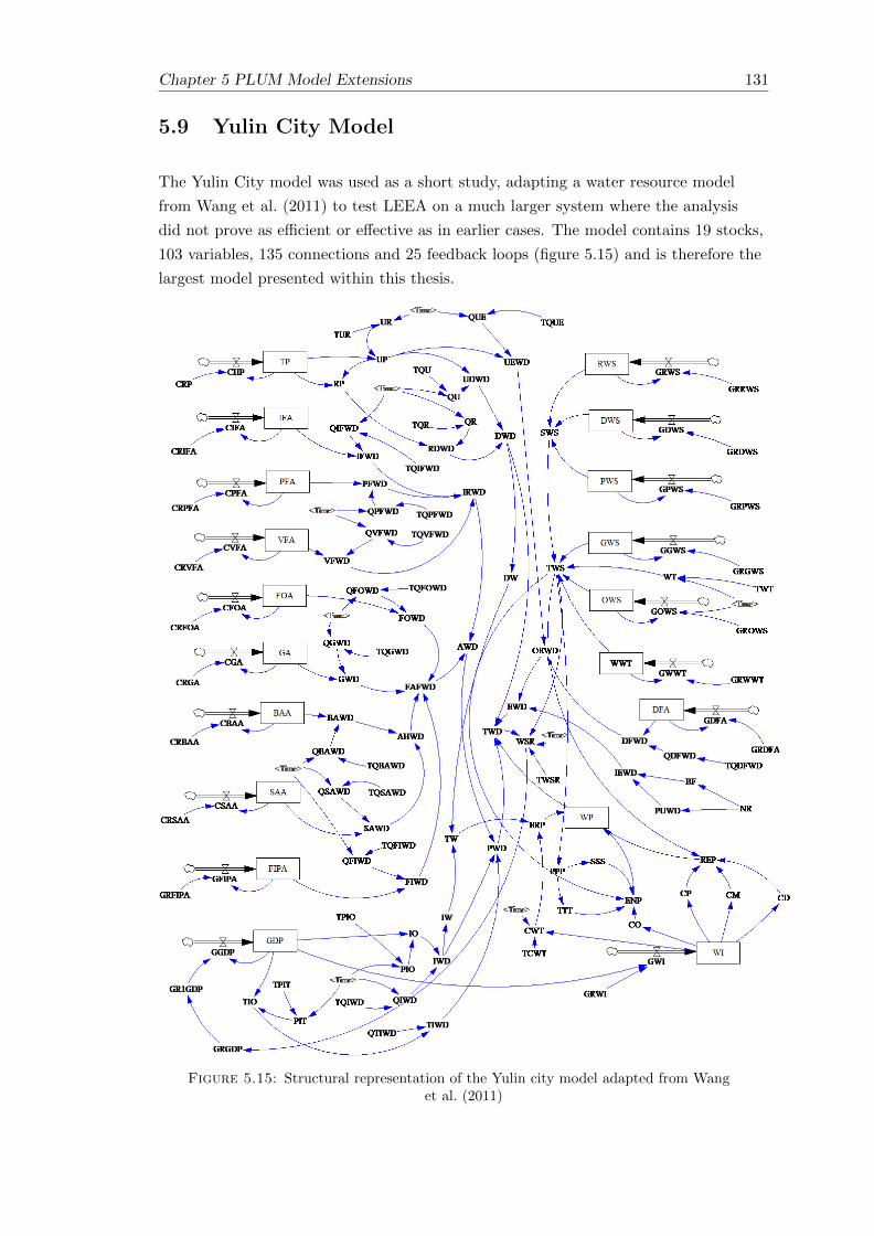
Chapter 5 PLUM Model Extensions 131
5.9 Yulin City Model
The Yulin City model was used as a short study, adapting a water resource model
from Wang et al. (2011) to test LEEA on a much larger system where the analysis
did not prove as efficient or effective as in earlier cases. The model contains 19 stocks,
103 variables, 135 connections and 25 feedback loops (figure 5.15) and is therefore the
largest model presented within this thesis.
Figure 5.15: Structural representation of the Yulin city model adapted from Wanget al. (2011)

132 Chapter 5 PLUM Model Extensions
LEEA was difficult to implement as many dynamical functions, including ‘IF THEN
ELSE’ statements within the model were incompatible with LEEA’s automated soft-
ware and had to be rewritten using graphical alternatives. Some of the Yulin model’s
structure had to be redesigned with the addition of interations to compensate for the
alternative functions. Alongside the effort required to make LEEA and the Yulin City
model compatible, the results showed limited use.
After processing, the graphical analysis section of LEEA identified that the loop to
stock ratio, 25:19, was low compared to other models were LEEA has proven success-
ful. Within the Yulin City model 16 out of 19 stocks were not linked through any kind
of feedback to the rest of the system, effectively making them linear inputs to a much
smaller set of feedbacks. As shown from the loop gain plot in figure 5.16, only one of
the 25 loop structures showed some form of spiking dynamic during the first seven
years of the simulation, with little changing in the rest feedback loops for the remain-
der of the time series.
LEEA can only account for the dynamics of a model which are taking place within
feedback loop structures. Since only three stocks of the model were intergral parts of
the main body of feedback structures, the information gained from LEEA could only
be attributed to the behaviour of 3 of the 19 stock variables. The output of the anal-
ysis therefore did not reflect the dynamics within the majority of stocks within the
model.
Figure 5.16: Loop Gain output from the Yulin City Model giving a first impressionof the dynamics and dominance of the 25 loop structures present within the system
prior to calculation of loop influence.
It is important to consider the volume of graphical output LEEA would produce for
the Yulin City model, despite only representing dyamics in 3 of the 19 model stocks.
Since there is a direct relationship of model stock number and eigenvalues calculated
for the analysis, the Yulin City model would have at the very least, 40 graphical out-
puts (1 eigenvalue plot, 1 loog gain plot, 19 loop elasticity plots and 19 loop influence
plots) needing to be prioritised for interpretation. This is a high volume of data con-
sidering it does not account for roughly 80% of the model’s stocks.

Chapter 5 PLUM Model Extensions 133
LEEA does have the potential to be used on models of high order, size and complex-
ity, but if such a model is not being built with LEEA in mind, then the user must be
ready to partially rewrite the model in order to run the analysis. The size of the Yulin
City model means that LEEA produces a large volume of graphical output, meaning
interpretation of the analysis could be time consuming for the amount information
gained. The low loop to stock ratio of the model means that the output of LEEA
would likely be as much of a ’black box’ to understand as the inner workings of the
model itself.
5.10 Discussion
Findings from the analysis of PLUMGov, PLUMPlus and Yulin models
The purpose of constructing and analysing the two extensions to the PLUM model
and of the analysis of the Yulin model was to investigate how interpretation of LEEA’s
output may become more complex with larger model size. The following discussion
points therefore concentrate on the interpretation of the analysis outputs more than
the specific dynamics expressed within the plots.
The PLUMGov model was created to show how the simple addition of an extra feed-
back loop could affect the interpretation of LEEA. While results remained relatively
simple to interpret with one dominant eigenvalue containing only two influential loop
structures, the addition of a balancing loop to counteract the system’s primary mech-
anism of instability generated oscillatory trends across the simulation and therefore
created complex numbers within the eigenvalues at and between the forward and re-
verse critical transitions which were not prominent within the original PLUM model.
The difference was dependent on whether reductions of phosphorus after the forward
critical transition were controlled by the active input of a user via a step fucntion at a
selected time step (as in the PLUM model) or by a reactive endogenous feedback loop
which contained a sigmoidal function (as in the PLUMGov model).
The PLUMPlus model was constructed in order to introduce a variety of new stocks
to the system alongside several new dynamics which added to and manipulated feed-
back loops currently operating within the PLUM model. Overall interpretation of the
results was still manageable, but addition of new stocks to the model brought with
them a multitude of new graphical outputs to be examined. In the original PLUM
model, three stocks meant that at most, 8 plots would have to be examined (1 eigen-
value plot, 1 loop gains plot, 3 loop elasticity plots & 3 loop influence plots), each
with 6 feedback loops with which to identify dominant drivers of system behaviour. In
comparison, the PLUMPlus model had seven stocks and its oscillatory trends meant
that a total of 31 plots would have been examined (1 Eigenvalue plot [real part], 1

134 Chapter 5 PLUM Model Extensions
eigenvalue plot [imaginary part], 1 loop gains plot, 7 elasticity plots [real part], 7 elas-
ticity plots [imaginary part], 7 influence plots [real part] & 7 influence plots [imaginary
part]), each with 17 different feedback loops with which to identify dominant drivers
of system behaviour.
An issue that might arise from a high number of system eigenvalues can be seen in
figure 5.13, where different dominant eigenvalues expressing completely different feed-
back loops are seen influencing the system’s behaviour. Both the PLUMGov outputs
and PLUMPlus outputs also show signs of ‘artificial loops’ or ‘ghost loops’, where
seemingly high influential loop structures are actually being counteracted by the dy-
namics of another loop and therefore are not contributing to the current behaviour of
the system.
The Yulin city model was the third example used within this study to evaluate a model
where LEEA may not be so appropriate. The Yulin city model’s structure is largely
designed around unidirectional connections between stocks which form a relatively low
number of feedback loops for the high number of stocks that it contains. This means
that any analysis obtained from LEEA would only be representative of a small sec-
tion of the model. In this case other analysis methods such as sensitivity analysis may
be more appropriate to identify key variables. The Yulin city model also took a long
time to adapt manually in order to carry out LEEA as many of the functions were not
compatible with the algorithms used to perform loop analysis. If LEEA is to be used
successfully on models of this size (19 stocks) it may save time for the model to be de-
signed with the application of LEEA in mind, though this is not usually the order in
which model construction and analysis tools are considered.
Physical limitations of the technique
One aspect of socio-ecological systems and the models which represent them is an as-
pect of choice and decision making that exists within the social side of the models.
Generally speaking, the idea of choice, or individuals within a system being able to
make their own, sometimes irrational, decisions is an integral part of an accurate and
justifiable SES model. In terms of running LEEA on such models, the analysis output
could still prove useful, helping to examine which feedback loops drive certain deci-
sions or sway a deciding vote. However, attention must be paid to the way that the
aspect of choice has been implemented within the equations of a model as this could
impact the extent to which LEEA could be utilised, or impact the manual labour time
required to adapt the model to be compatible with LEEA. As an example, IF and IF
THEN ELSE statements are often used to segregate a population between alternative
decisions, but these statements are not compatible with current versions of the LEEA
online utility algorithms (Naumov & Oliva 2017).

Chapter 5 PLUM Model Extensions 135
In order to address the lack of automation of the technique, Naumov & Oliva pro-
vide a worksheet in Mathematica to help users through the main steps on the analy-
sis (Naumov & Oliva 2017). This has greatly streamlined the mechanical running of
LEEA. However work must still go into preparing a system’s model and its data out-
put in order to use the worksheet and the code must be manipulated in order to gain
Elasticity and Influence output plots.
Validation of results
As stated previously within this case study, values for system components of the PLUM-
Gov and PLUMPlus models either stem from the original Carpenter model, or have
been chosen arbitrarily for the purpose of analysis exploration. When working with a
real system and in order to get the most out of loop analysis, all system components
must be validated empirical data if any comparisons are to be made back to the real
world system from which the model derives. However, the validation of system compo-
nents and its output is a universal issue, with the field of ecology being no exception.
Data collection for key system components can be impractical or economically unvi-
able to acquire, making validation fitting techniques difficult to achieve. Validation of
model outputs may also be impractical as they require manipulation of the real world
system in order to test results, which may not be feasible.
Interpretation error
The dynamics within PLUMGov and PLUMPlus are interesting for their loop influ-
ence plots because the behaviour, system mechanisms and build-up to each critical
transition can be observed changing through time leading up to each event. Observing
how the trajectories of eigenvalue and loop influences changes through time is an im-
portant part of the analysis process as it can give clues as to the change of an eigen-
values polarity or the dominance a loop structure might gain further along the time
series. However, there is an interpretation error associated with eigenvalue and loop
influence line plots which increases as the time step between the points calculated for
LEEA increases. The linearization process for calculating the system’s Jacobian Ma-
trix treats each point in time as a completely separate event so making interpretations
between these points can lead to inaccuracies in interpretation. To overcome this,
when possible, the time steps taken for LEEA can be reduced, decreasing the time
between calculations and increasing the number of individual events calculated within
the analysis. The user can also inspect each point in time on eigenvalue and loop in-
fluence plots individually, which is more time consuming, but completely removes this
type of interpretation error.
Regarding safe and just operating space
Working within a safe and just operating space is a primary concern within the fields
of sustainability, resilience, conservation and recovery, where many ecological and

136 Chapter 5 PLUM Model Extensions
socio-ecological models stem from. LEEA is purely based on numerical techniques and
mechanical responses; it therefore has no regard for operating within a socially accep-
tible and economically viable space, unless these concepts are integrated as part of
the analysed model. It would therefore be discouraged to base policy changes and lo-
cal decisions on structural analysis alone as its output should be considered alongside
what is safe and just for the system and its inhabitants.
Future work
While LEEA has proven to be a promising technique for understanding socio-ecological
dynamics, more experimentation needs to be conducted on it in order to understand
its capabilities. By utilising structural loop analysis, sensitivity analysis could be run
to investigate changes in loop magnitude, loop polarity and the order of loop domi-
nance. This would not only identify which system components are having the great-
est impact on behaviour, but also which mechanisms present in the model are allow-
ing them to do so. This would mean measuring complexity not just by the number of
variables, but the loops that they create. Using SILS to analyse loop structures would
allow for the presence and abundance of feedback loops to be considered as a quantifi-
able level of complexity within system dynamic models in a similar way to how cen-
trality, node connectedness and clustering are all concepts of complexity in network
modelling (Costa et al. 2007; Dunne et al. 2002). Making loop analysis techniques a
common practice through further development and automation, could have profound
implications for the way that we approach model simulation, while also increasing
model efficiency and understanding.
5.11 Concluding Statements
LEEA, in its current stage of design, is not an appropriate method for all dynamic
system models. Its main limitations prevent it from lifting the black box away from
large system models, outputting results which can be just as incomprehensible as the
system which it is attempting to analyse. While the technique and methodology be-
hind LEEA may improve with future iteration of the technique, its design is based
around the analysis of feedback structures, meaning that there will be some system
models where its practical application will never provide the user with novel informa-
tion about the target system.
While feedback loops act as key driving mechanisms in practically every known sys-
tem, models do not have to be designed in a way to best express dynamics via feed-
back structures, thus limiting LEEA’s ability to analyse the link between system struc-
ture and system behaviour. With regards to model size, LEEA is physically capable of
being carried out on any system model it has been presented with, but it is the user’s
ability to interpret LEEA’s results that can run into difficulty. Using LEEA on large,

Chapter 5 PLUM Model Extensions 137
highly complex models becomes less of a pragmatic problem, if the user is 1) familiar
with the outputs of LEEA and how to interpret them, 2) familiar with the target sys-
tem, able to apply LEEA’s outputs back to the model, 3) has time available to review
all of the output LEEA is able to produce from a single simulation.

138 Chapter 5 PLUM Model Extensions
Chapter 6: Chapter Preface
Loop Eigenvalue Elasticity Analysis (LEEA) has been shown to have utility on a small
dynamic lake model as well as being effective at analysing structural feedback loops
driving critical transitions. Alongside investigating limitations of LEEA it is impor-
tant to gain a greater understanding of how model properties (dynamics, structure
and values) relate to LEEA output and vice versa. Determining the most dominant
feedback loops in a system is a valuable asset to a model analysis, but understanding
how sensitive a loop’s dominance is to changes in model parameters can also be valu-
able when attempting to maintain or manipulate a behaviour or outcome.
Within this chapter, the meta-analysis of LEEA is continued to examine LEEA in
the context of analysis sensitivity. Here, the extent to which a model parameter’s
value must be changed in order to cause change within the loop dominance outputs of
LEEA is assessed. Conducting sensitivity analysis, not just on a model system, but on
the analysis outputs allows a greater connection between model properties and LEEA
results to be understood. Investigating a system’s sensitive parameters in the context
of dominant loop structures gives a greater understanding of potential leverage points
within the system, which allows a connection to be drawn between LEEA implementa-
tion and policy design based on structural drivers of system behaviour.
Chapter 6
Accessing LEEA’s Niche: An
Analysis Comparison in the
Context of Leverage Points
6.1 Abstract
System dynamic models are not commonly used for their predictive capabilities, nor
to output exact values of given parameters. Instead, their strengths lie in simulating
trends in model behaviour and can be used as a base with which to test the imple-
mentation of new policies, before they are implemented on a real ecosystem. Com-
bined with the methodology from Loop Eiganvalue Elasticity Analysis (LEEA), sys-
tem dynamic models could be used to identify leverage points of a system, identifying
structures, or variables with the greatest ability to induce change to a system’s be-
haviour when perturbed. The identification of leverage points is considered a valuable
output of model analysis in light of environmental conservation, control and recovery.
Structural loop analysis of dynamic socio-ecological models has been shown to be a
unique tool for quantifying a feedback loop’s influence over a system’s behaviour. The
output of LEEA allows the user to identify dominant loop structures, controlling the
system’s current behaviour and rank their influence against other feedback structures
within the model. Identifying dominant structures of model behaviour is a valuable
tool for testing and designing model scenarios, but LEEA also has potential for use
in policy design and implementation when used alongside its partnering analysis Dy-
namic Decomposition Weights Analysis (DDWA).
This study discusses the ability for structural loop analysis to aid in the identification
of leverage points within a dynamic model system. As part of the discussion, LEEA
139

140Chapter 6 Accessing LEEA’s Niche: An Analysis Comparison in the Context of
Leverage Points
is assessed for its sensitivity to changes in model parameters and as part of a meta-
analysis of LEEA, we test how liable the leverage points of a system are to change
with different parameter starting values and trajectories through time. The discussion
considers whether LEEA can be an appropriate method to help guide policy as an in-
dividual technique or as part of a toolset combined with other analytical methods.
The results show the application of structural loop analysis to leverage point iden-
tification will question our ability to manipulate system variables over our ability to
manipulate entire feedback structures within socio-ecological systems.

Chapter 6 Accessing LEEA’s Niche: An Analysis Comparison in the Context ofLeverage Points 141
6.2 Introduction
The use of system dynamic models to portray ecological and socio-ecological systems
(SES) alongside the results of Loop Eigenvalue Elasticity Analysis (LEEA) allow us
to explore and understand a system’s internal structures as drivers of endogenous dy-
namics, forming a cognitive link between system structure and system-wide behaviour.
In order to further utilise these techniques in the context of modern requirements,
such as system maintenance or system recovery, we must be able to utilise the anal-
ysis results in a way that is able to enhance and inform environmental policy.
A natural step in the process of understanding a socio-ecological system is how we can
use knowledge over the system to adapt current policy and future legislation. By uti-
lizing LEEA, whose analysis gives us greater information about behavioural influences
and system drivers, there is great opportunity to design policy based on targeting spe-
cific feedback mechanisms with the intent of having the greatest impact for the time
and effort put in.
The purpose of this chapter is to continue the meta-analysis of LEEA from previous
chapters with an extension known as Decomposition Weights Analysis (DDWA) (Oliva
2015; Saleh et al. 2010) and combine the two techniques with that of a commonly used
analysis tool within system dynamics and socio-ecological systems, Sensitivity Analy-
sis (SA). While the analysis tools have similar purposes; to identify and rank impor-
tant features within a system, they go about it in different ways. Sensitivity Analysis
considers system parameters as individual sights for system sensitivity, while LEEA
and DDWA focus on the interactions between components.
The theory and application of all three methods, LEEA, DDWA and SA, is used to
bridge the gap between sensitive model components, structural drivers and policy im-
plementation. By a comparison which takes into account all three analysis techniques,
this study opens up a discussion as to how such techniques can be used to identify
leverage points over a system’s behaviour. It is speculated whether it is possible to
gain a deeper understanding of system drivers and a stronger ability to manipulate a
system in an effective way when these techniques are combined together, as opposed
to viewing them as separate choices in model analysis.
In this study LEEA, DDWA and SA are carried out on the same model system. Each
analysis is connected by their ability to identify and rank the influence or sensitivity
of system components, be they in the form of individual variables or loop structures.
LEEA and DDWA are linked further as they both stem from the same line of graph
and linear analysis theory. LEEA can be used to identify loop structures driving the
overarching behaviour of a system, while DDWA links parameter change to individ-
ual system stocks. Sensitivity analysis is a more commonly known technique, used to

142Chapter 6 Accessing LEEA’s Niche: An Analysis Comparison in the Context of
Leverage Points
identify parameters of a system which the output is most sensitive to and can be ap-
plied at a local (one parameter at a time) or regional (multiple parameters simultane-
ously) scale. The techniques are compared and contrasted for the components which
they identify as the most important to a system’s behaviour.
This experiment has multiple purposes:
1. To investigate whether there is a link between sensitive variables identified within
SA and influential loop structures identified within LEEA. Do the analysis tech-
niques agree or complement each other and would it be beneficial to use both of
these techniques during model analysis of future modelling practices?
2. Do variables which are contained within the most influential loop structures out-
put as highly influential variables when analysed at an individual level?
3. Sensitivity degrees of system parameters reflect on the parameter’s influence on
the overall system’s or a stock’s output, but will changes to parameters with
high sensitivity degrees also reflect a high impact on loop dominance within the
system?
4. Bridging the gap between model analysis and policy implementation: what does
LEEA provide within the context of current analysis techniques and how appli-
cable is it to reflecting on real world systems, identification of leverage points
and policy implementation over these systems? Does LEEA perform well within
a niche that is currently lacking within the ecological modelling process?
Using the three techniques in tandem, on the same model system and comparing re-
sults will allow us to test which parameters and loop structures within the system
individual stocks are most sensitive to. Identifying which parameters each technique
outputs as a key driver of model behaviour will allow for a critical analysis of LEEA
against other techniques. The study will also provide a base with which to test the
sensitivity of LEEA’s outputs and a platform with which to discuss the identification
of system leverage points and incorporate LEEA as part of a policy design process.
6.3 Background
The following section breaks down current knowledge and practices surrounding sensi-
tivity analysis and system leverage points.
System Leverage points
Within this study, LEEA is examined for its potential use in policy. In order to bridge
the gap between the graphical outputs of LEEA and the practice of making effective

Chapter 6 Accessing LEEA’s Niche: An Analysis Comparison in the Context ofLeverage Points 143
policy, LEEA’s output is justified in the context of system leverage points. Mead-
ows (2008) states that the applications of model output and analysis to inform policy
should be conducted through the discussion and identification of leverage points.
Leverage points are defined as “Places within a complex system(a corporation, an
economy, a living body, a city, an ecosystem) where a small shift in one thing can pro-
duce big changes in everything.” (Meadows 1999). Leverage points are often linked to
feedback loops generating behaviour and can be sought after to address detrimental
system behaviour. Meadows talks about using leverage points to influence our policies
and LEEA could provide a method to identify a system’s most influential components.
Leverage points are not a recent or novel idea and have been embedded into folklore
and legends for centuries as the single hero, villain or one defining act that turns an
entire story on its head. In the context of complex and dynamic systems, leverage
points come in multiple forms, all of which are identified as a means to generate sig-
nificant change in the target system. Meadows (1999) identifies twelve possible areas
within a complex system which can be identified as leverage points. Two of those
twelve are directly related to system feedback loops and our ability to manipulate
them:
Leverage point no. 8; “The strength of negative feedback loops relative to the impacts
they are trying to correct against.” (Meadows 1999)
Leverage point no. 7; “The gain around driving positive feedback loops.” (Meadows
1999)
Despite it being known for decades that feedback loops are one of the key components
for manipulating and controlling system behaviour, the identification of the loop struc-
tures within systems and the significance of each loop has been difficult to ascertain,
until now. LEEA has the potential to idenitfy feedback loops which, in the context of
Meadow’s points 7 and 8, could be leverage points to the system.
Caution must be taken when identifying leverage points as they cannot be considered
the be all and end all of informed political decisions. Leverage points may not always
be accessible, even if they are known and we are informed enough to know which way
to push them (Meadows 1999). Leverage points must be identified for their effective-
ness and efficiency at manipulating the desired system or a desired parameter as po-
tentially all parts of a system could be regarded as a point of leverage. Some will be
more effective than others.
The identification of leverage points in a system should be of high importance to any
model analysis where the end goal of the user is to manipulate the system. While
leverage points within a model system could mean the deliberate change to a param-
eter’s value, they may also come in the form of an entire feedback structure which

144Chapter 6 Accessing LEEA’s Niche: An Analysis Comparison in the Context of
Leverage Points
holds dominance over the system. While LEEA allows us to identify dominant feed-
back loops within a system structure, it is limited in its ability to offer knowledge of
how to best manipulate and lever those loop structures.
The multiple uses of sensitivity analsyis:
Sensitivity analysis, when used within an ecological context, can determine the rela-
tive importance of parameter input values on the output of the model. Cariboni et al.
(2007) discuss a range of questions which sensitivity analysis can be used to answer. A
breakdown of Cariboni et al.’s discussion on the uses and capabilities of SA are listed
below:
• For determining the influence of uncertain variables where the evidence sur-
rounding them may not be strong.
• Identify variables which the system is highly sensitive to while also identify-
ing highly uninfluential variables. It is therefore possible to use SA at various
steps along the modelling process. It can help to determine inputs which could
be eliminated as they contribute little to no input to the variance of the model
output, simplifying model structure.
• Identify areas of the model which may wish to be expanded upon, if the analysis
identifies a variable which the model is particularly sensitive to, it could indicate
some key dynamics/ variables missing from that part of the model.
• Able to identify if there are ranges of values which a variable can be changed
within without affecting the model results.
• Able to identify input combinations which could be classified as high risk within
the output parameter space.
• Used to identify interactions between variables.
• Help determine specific goals of research.
• As a method to measure whether the model accurately reflects observations and
data from their real-world ecosystems.
One particular use of sensitivity analysis, known as factor prioritisation, is performed
post model construction, once the model has been validated and all values are as-
sumed to be true or lie in a range that reflects the system of the real world ecosystem.
The outcome of SA in this context allows the user to identify the most influential fac-
tors corresponding to the model’s output. In factor prioritisation, factors are identified
and ranked in order of most deserving to re-measure in order to reduce model variance
(the spread of a set of data from its average) (Cariboni et al. 2007).

Chapter 6 Accessing LEEA’s Niche: An Analysis Comparison in the Context ofLeverage Points 145
A second, or rather continuation of factor prioritisation allows for the identification
of highly uninfluential factors. Cariboni et al. (2007) relay uninfluential factors of a
model as ones who can be given any fixed value within their domain without having
any impact on the model output i.e. without contributing to a reduction in model
variance.
From the above examples, it is easy to draw similarities between SA and LEEA. Both
SA and LEEA can take on similar roles in the identification of highly influential and
non-influential model components. Both techniques are also able to rank the influence
of their corresponding findings in order to produce a priority list for system parame-
ters. The ranking system produced from either method can also be used to increase
the efficiency of carrying out model simulation, or re-building by identifying low influ-
ence factors which can largely be ignored, or should be considered to remove from the
model in order to reduce model size, and increase efficiency.
The main difference between SA and LEEA is what they identify and class as influ-
ential. SA mainly concentrates on factors at an individual level or multiple factors
together that don’t necessarily contain a link between them, while LEEA is designed
to only focus on feedback loop structures. SA can be run on every variable within a
model to test its input vs the sensitivity of model output, while LEEA will only con-
sider a particular variable if it is an integral part of a feedback loop. Both analyses
have their respective advantages and disadvantages. SA, when performed at a local
level (one-at-a-time) does not take into account any dynamics within a model as it
solely focuses on the input of an individual variable. At a global level in SA, when
multiple factors are tested simultaneously, links between variables can be inferred,
hinting at some dynamics properties of the model, but this does not equate to the
identification of entire feedback structures, which LEEA specialises at analysing. How-
ever, LEEA is incapable of measuring the impact of variables which act exogenously
to the dynamics of a system’s feedback structure.
It is within these similarities and differences between LEEA and SA that the study
will cross compare the technique outputs. As SA is already an established method
within the field of socio-ecological studies (Kioutsioukis et al. 2004; EPA 2003; Zal-
divar and Campolongo 2000) it is seen as a beneficial exercise to compare LEEA re-
sults in order to show its relevance to the field and ground it with context against a
well-known and well used method.
Examples of SA being used within the field of socio-ecological systems include Chap-
man and Darby (2016) and Zhang et al. (2008), who use sensitivity analysis to test
their system’s response to changes in variable input values. Chapman and Darby (2016)
use sensitivity analysis on five system parameters whose attributed values are “no-
tably weak evidence based”, meaning that the sources of their values were not as re-
liable or validated to the same extent as others within the model. Chapmann and

146Chapter 6 Accessing LEEA’s Niche: An Analysis Comparison in the Context of
Leverage Points
Darby used sensitivity analysis to explore the system’s sensitivity to these five param-
eters and in doing so evaluate their confidence in the model.
6.4 Methodology
The methods section covers the analysis techniques, DDWA and SA, to be used and
compared alongside LEEA.
Dynamic Decomposition Weights Analysis (DDWA)
Associated with LEEA is a technique known as Dynamic Decomposition Weights
Analysis (DDWA) (Saleh et al. 2010), which has been designed to increase the rel-
evance of LEEA’s output to policy. While LEEA provides a method with which to
develop an understanding of system behaviour which is based on endogenous system
drivers, DDWA has been developed for more policy-orientated requirements (Oliva
2016). From linear systems theory, the behaviour of a given stock can be expressed as
the sum of each eigenvalue within the system, each carrying a different weight which
they have over that stock at any point in time (Saleh et al. 2010). A higher weight in-
fers a greater expression of the eigenvalue’s output within the behaviour of the system
stock of interest. DDWA analyses what happens to the weights of eigenvalues when
parameter values within the models change through time. Unlike LEEA, the weights
within DDWA are specific to each stock and help to gain an idea of which parameters
are holding the greatest impact on the system at specific points in time. The results of
DDWA will also be conducted within this study and discussed alongside the results of
SA and LEEA.
The main role of both LEEA and DDWA is to assess the role of endogenous drivers of
a system. DDWA acts as an extension to the methodology conducted within LEEA.
Where LEEA analyses the influences which feedback loops have on the entire system,
DDWA is able to relate the influences on stock variables to individual parameter val-
ues. In doing so, DDWA allows system drivers to be identified at a parameter based
level, a level on which policy discussion and implementaion is usually based. Along-
side LEEA, the output from DDWA allows not only for highly influential loop struc-
tures to be identified, but determines which parameters within those loop structures
are best to target if the behaviour of a desired stock is to be changed.
A system dynamic model can be translated to a pure mathematical form as a set of
nonlinear differential equations. LEEA and DDWA both rely on the system they are
analysing to be linearized, but it is rare to find a model system, particularly in the

Chapter 6 Accessing LEEA’s Niche: An Analysis Comparison in the Context ofLeverage Points 147
field of SES, that can simulate the behaviour of its target system without using non-
linear equations. In order to accommodate for this, a model’s behaviour may be ap-
proximated around any one point in time as a set of time-invariant linear differential
equations as described in Saleh et al. (2010).
The weights within DDWA are calculated as a function of the system’s eigenvectors.
Dynamic Decomposition Weight Analysis (DDWA) was originated within Saleh et al.
(2010) developed from the works of Goncalves (2009), who extended the eigenvalue
elasticity approach to focus on the trajectory of individual stocks. When focusing
solely on the endogenous dynamics within the system, the exogenous variables can be
set to zero or constant. With no exogenous drivers influencing system behaviour, the
resulting output of each stock can be written as a weighted sum of all the behaviour
modes (eigenvalues) within that system:
xi(t) = wi,0 + wi,1eλ1t + · · ·+ wi,ne
λnt (6.1)
Where xi(t) is the resulting behaviour of the state variable, w are the weights associ-
ated with each eigenvalue which are constants dependent on the eigenvectors and the
initial conditions of the system and λ are the eigenvalues of the Jacobian matrix (see
Saleh et al. 2010 for the derivation). DDWA is concerned with the weights w, of the
above equation as the system changes through time. Similar to the output of LEEA,
the relationship between the changes made to individual elements, a, of the system
matrix and the weights, w, can be calculated either as elasticity measurements εw, or
as influence uw.
εw =∂w
∂a.a
wand uw =
∂w
∂a.a (6.2)
A major difference between LEEA and DDWA is that LEEA only takes into account
parameters and connections that form part of loop structures, while DDWA analyses
all links within a system’s structure as every link has potential relevance.
The weight of an eigenvalue to any given stock is not static and is able to vary with
changes which occur in other parameters of the model. The connection between a
changing parameter and the elasticity of an eigenvalue’s weight can be assigned a
value. The magnitude of the value (as an absolute number) reflects the level of im-
pact that the parameter will have on the weight of an eigenvalue and by knowing this,
it is possible to link parameter change with eigenvalue weight and therefore parame-
ter change with stock behaviour. The polarity of the elasticity indicates whether the
parameter will increase or decrease the weight of the mode for that stock. If the elas-
ticity value is positive then an increase in the parameter corresponds to an increase in

148Chapter 6 Accessing LEEA’s Niche: An Analysis Comparison in the Context of
Leverage Points
the weight. If the elasticity value is negative then an increase in the parameter corre-
sponds to a decrease in weight.
Saleh et al. (2010) point out that DDWA allows for the user to rank the influence of
each parameter within the model in the search for potential leverage points, with-
out the need for multiple scenario testing. This makes the DDWA efficient, especially
when used on larger models where scenario testing and model runs can be time con-
suming.
Sensitivity Analysis
System dynamic models are made of four components, stocks, flow rates, auxiliary
variables and constants. Of those, stocks are determined by input and output flow
rates and rates are determined by auxiliary variables and constants. Constants and
auxiliary variables in the model can be run under sensitivity analysis. The values as-
sociated with these variables are common places where uncertainty can occur and are
areas for potential error within a model. Sensitivity analysis on these variables can
be used to test how sensitive a model output, or an individual model parameter (i.e.
a system stock) will be to a change in these variables. Sensitivity analysis can not
only be used to identify how sensitive an individual parameter is, but also the whole
model’s output. This sensitivity associated with each variable is given a number called
its sensitivity degree.
A parameter’s sensitivity degree can be calculated manually, through dynamic mod-
elling software STELLA or Vensim PLE Plus. Vensim PLE Plus requires a license,
but whose cost is reduced if being used for academic purposes. Any variable with a
sensitivity degree of > 0.1 is seen as a highly sensitive variable. Using sensitivity anal-
ysis the user is able to identify ‘system sensitive parts’ (Zhang et al. 2008) i.e. com-
ponents of the system whose output is affected the most by the change of a variable’s
input.
A common way to quantify sensitivity analysis within system dynamic models is by
calculating the sensitivity degree associated with each variable. The sensitivity degree
is how sensitive a parameter (stock) or the system as a whole is to that variable. Sen-
sitivity degree (SQ) takes the following form:
SQ = |∆Q(t)
Q(t).X(t)
∆X(t)| (6.3)
where t is time; Q(t) is the model output of a stock at time t; X(t) is the input of the
variable being tested for sensitivity at time t.
When a sensitivity degree can be gained for each stock in the system, an average of
these degrees taken across all stocks will give the general sensitivity degree. The gen-
eral sensitivity degree of a variable shows how sensitive all system stocks are combined

Chapter 6 Accessing LEEA’s Niche: An Analysis Comparison in the Context ofLeverage Points 149
to that variable which is another way of saying how sensitive is the system as a whole
to that variable. For n system stocks, (Q(1), Q(2), Q(3) . . . Q(n)), the general sensitivity
degree of a variable is calculated by the following:
S =1
n.n∑i=1
SQi (6.4)
Where S is the general sensitivity degree of n stocks to the variable being tested; S(Qi)
is the sensitivity degree of the variable being tested to stock Q(i) as seen in equation
6.3.
Meta Analysis Breakdown:
1. DDWA is run on the PLUM model to identify which parameters each stock is
influenced by the most throughout the simulation.
2. Sensitivity analysis is run on each individual variable within the PLUM model
system to identify which register as highly sensitive or critically sensitive vari-
ables via their sensitivity degree.
3. Results are compared to that of LEEA from previous chapters to see if the vari-
ables picked out by the sensitivity analysis are the same variables that are part
of the most influential loop structures from structural loop analysis (LEEA).
• If the same variables appear sensitive as the variables involved within the
influential loops of LEEA then a comparison can be drawn as to whether
the analysis methods complement one another.
• If results are different, it is possible that local SA is not able to pick out
the interactions between variables and therefore is not representing the dy-
namic properties that are present within the model.
4. A set of variables are determined based on the results of SA and DDWA. The
results are used to design multiple scenarios, testing changes within model vari-
ables against the output of LEEA and the influential loop structures. Scenarios
which then produce results of particular interest are selected to evaluate within
the results. Questions during scenario testing include: Is there any way of caus-
ing the hierarchy of loop dominance to change regarding a key behavioural dy-
namic such as a critical transition? Will the change required to force a change
in a dominant feedback sit within a realistic spectrum of natural phenomena or
human ability?
The goal is to investigate how much impact on the model’s most sensitive variables is
required to change the influence of loops within the system and investigate whether

150Chapter 6 Accessing LEEA’s Niche: An Analysis Comparison in the Context of
Leverage Points
there is a link between sensitive variables and dominant loop structures. In order to
achieve this, an individually sensitive or multiple sensitive variables are selected from
SA and changed by orders of 10-40% to generate different starting conditions for the
PLUM model system. Variables which are not selected to be changed are kept at their
values from the base scenario. Each new set of starting conditions will generate differ-
ent scenarios and model outputs. Each of these scenarios is then analysed using LEEA
in order to calculate the influence of loop structures within the new scenario. This
process will also be tested on variables which were identified as uninfluential or having
a low sensitivity degree. The outputs of LEEA will be used to compare and contrast
any changes which occur from the original scenario of the PLUM models forward crit-
ical transition, as explored within chapter 4. This experiment investigates how much
the initial conditions of the PLUM model must be manipulated to start seeing a dif-
ference in output plots of loop influence, giving some indication on the relationship
between parameter starting values and the consistency of the outputs we might expect
from LEEA.
Local SA for PLUM model
Sensitivity analysis has been conducted on the PLUM model. An initial sensitivity
analysis of the PLUM model was conducted over the region of 250-1000 years. Start-
ing at 250 years, each parameter within the model that acts as either a constant or an
auxiliary variable was set to vary by 10% by the end of the simulation. The analysis
was conducted at 250 time steps to avoid any changes which were introduced to the
system regarding agricultural and non-agricultural changes prior to the critical transi-
tion, avoiding the manually implemented step function within the dynamics as this is
incompatible and poses a physical limitation of the online software of Naumov & Oliva
(2017).
Time steps for calculating a variable’s sensitivity degree are chosen relative to the to-
tal number of time steps i.e. 750 time steps between 250 and the end of the simula-
tion at 1000 is broken into points at 250, 400, 550, 700, 850 and 1000. Between each
section (i.e. 250 to 400) the value of one parameter of the system increased by a set
amount, 2%. For each section after, the same parameter is increased by a further 2%
from the last to create a linear increase of the parameter through time, up to a total
of 10% increase from the original.
A sensitivity degree was then recorded for each value at a 150 time step interval for
both the system’s manually changing input parameter X and the affected output stock
parameters Q, (equ. 6.3). This calculates the relative change in parameter Q in re-
sponse to changes in X. A sensitivity degree value can then be calculated from each
time section through equation 6.3. A general sensitivity degree can then be calculated
as an average across all time sections.
Chapter 6 Accessing LEEA’s Niche: An Analysis Comparison in the Context ofLeverage Points 151
6.5 Results
The results section breaks down the meta-analysis into three sections;
The first concerns DDWA conducted on the PLUM model, investigating which system
variables are identified as highly influential to the stock concerning phosphorus den-
sity within the lake water (P ). The stock P is focused on as this is where the system’s
critical transition occurs within the model.
The second section shows SA conducted on the PLUM model, primarily at a local
level, identifying which variables of the model have a high sensitivity degree. In both
sections, once each of the system variables have been assigned a value representing its
influence, or sensitivity degree, the levels of importance are cross compared with the
most influential loop structures identified with LEEA.
The third section invokes changes to the base PLUM model’s forward critical tran-
sition, where the system is manipulated based on the influential or sensitivity results
gained from DDWA and SA. Each new version of the model is then run through LEEA
in order to test the sensitivity of LEEA’s outputs to changes in the model system.
The outputs of LEEA on the new model simulations are displayed in graphical form.
The changes which are highlighted from each output are based on the most important
information which LEEA can provide to a user about their system, namely:
1. How many Loops display as influential and therefore hold some form of control
over the system’s behaviour.
2. How many loops are generating stability and how many are generating instabil-
ity, which loops are they and how do they compare across all model scenarios?
3. Which loops generate the highest absolute values of system influence and are
therefore deemed as the ones with the most contribution to the system’s be-
haviour? Are the highest influential loops consistent regardless of the system’s
initial conditions provided it always expresses the same dynamics?
Results: Dynamic Decomposition Weights Analysis (DDWA)
DDWA is able to weight each eigenvalue to a specific stock within the system. From
the PLUM model each stock can be plotted regarding the order which eigenvalues
influence that stock. DDWA is conducted at individual points along a time series to
identify which parameter values are most influential to a stock at that point in time.
In the PLUM model, the main concern of the system is the critical transition which
it undergoes into undesirable eutrophic conditions. DDWA has been conducted prior
to the forward critical transition of the system in order to assess which parameters
are most influential on the stock ’Pwater’ before the system undergoes a change of

152Chapter 6 Accessing LEEA’s Niche: An Analysis Comparison in the Context of
Leverage Points
state. The stock ’Pwater’ is chosen as the stock of interest as it represents the levels of
phosphorus within the water level, which are tied to the eutrophic transition and have
been shown to be part of the most influential positive feedback loop within the sys-
tem from chapter 4. The following plot (6.1) shows the weightings of each eigenvalue
through time as a projection of the system’s conditions from t=250 which correspond
to the stocks Usoil, Pwater and Msediment. The relative influence of each eigenvalue
have been normalised against a constant term (shown by the blue dashed line) in or-
der to make the influences comparable.
Figure 6.1: Eigenvalues weights from DDWA of the PLUM model at t=250

Chapter 6 Accessing LEEA’s Niche: An Analysis Comparison in the Context ofLeverage Points 153
In each plot above, the relative influence of each eigenvalue on each individual stock
can be seen through time by its associated absolute value. Unlike the entire system,
whose overall behaviour was largely described within eigenvalue 1 (dotted orange line),
we see that the behaviour of the ’Pwater’ stock at this point in time is largely gov-
erned by eigenvalue 3 (solid orange). From LEEA, we see that at this point in time,
eigenvalue 3 is dominanted by the stabilizing influence of loop 1, concerning the burial
rate of phosphorus (see figure 6.2). It is therefore no suprise that the most impactful
parameter at this point in time is parameter b, the permanent burial rate of sediment
phosphorus (years−1) (see table 6.1). It is using this information, that a deeper con-
nection between individual model parameters and stocks can be established.
The elasticity of DDWA weight values can be calculated for each system parameter.
The following table (6.1) expresses the estimated effect which each system parameter
has on the elasticity of eigenvalue 3 for Pwater at time t=250. The parameters are
ordered in descending order of elasticity. The values reflect the extent and manner
which a change in the parameter will generate a change in the associated stock.
Figure 6.2: The PLUM model in system dynamic form
To highlight what DDWA is able to show us figure 6.3, below, shows what the elas-
ticity values assigned to each variable mean when they are related back to a model

154Chapter 6 Accessing LEEA’s Niche: An Analysis Comparison in the Context of
Leverage Points
Table 6.1: DDWA elasticity values for each variable within the PLUM model ofChapter 4, for the Pwater stock (phosphorous density in lake water)
stock. In the Plot, parameter m (2nd highest elasticity, negative polarity parameter)
has been compared against parameter r (4th ranked elasticity, positive polarity) whose
elasticity is a magnitude lower. The absolute value of the elasticity shows the relative
impact of that parameter. As can be seen on the plot, increasing or decreasing m by
10% causes a much greater impact to the occurrence and level of the critical transi-
tion in stock P than increasing or decreasing r by 10%. The polarity of m is negative,
meaning that an increase in the parameter should decrease the weight of the eigen-
value, in this case , meaning the critical transition occurs much later in the time se-
ries. On the reverse, r has a positive polarity, meaning that an increase to r will in-
crease the effective weight of the behaviour mode, which in Pwater causes the critical
transition to occur much sooner.
As the system gets closer and closer to the forward critical transition, the weights of
the eigenvalues and their projections change, depending on the desired time chosen.
The critical transition of the system occurs between t=450 and t=460. At timestep
400, weights of the eigenvalues and their projections of stock Pwater have changed.
At t=400, the weight of eigenvalue 2 on the Pwater stock has increased to positive
values and is impacted purely by parameter c carrying an elasticity value of 1, while
the order of impact from parameters in eigenvalue 3, which still holds a large nega-
tive weight ranks in the following order (descending impact): m (-1.8262), b (0.8874),
q (-0.7971), r (0.2380), s (-0.1957), h (0.0709) and W,H,F and c (0). If this is the
desired time of interest, both eigenvalues 2 and 3 should be considered for their pa-
rameter elasticity values as they are weighted roughly the same. This exercise can be
conducted as any point along the time series, which in reality, would largely be deter-
mined when requirements of manipulating the system with use of policy change would
first be realised.

Chapter 6 Accessing LEEA’s Niche: An Analysis Comparison in the Context ofLeverage Points 155
Figure 6.3: An example of how elastcity values from DDWA reflect back on modeloutput, represented using variables m and r. Variable m has a high elasticity valuewhich is negative so a 10% change can makes large differences to the output, whilevariable r has a low elasticity, which is positive so a 10% change makes a relatively
small difference to model output.
LEEA allows for important loop structures to be idenitified from a structural model,
while DDWA allows the user to identify which parameters within those loop struc-
tures are generating the greatest impact to a corresponding stock. In the analysis of
the PLUM model, we know from LEEA that loop 5 (the phosphorus recycling loop)
was a key loop in the critical transition of this system. DDWA shows that as the pa-
rameters directly connected to that loop structure change and the system nears its
critical transition, the influence of each paramter can be determined by the absolute
value and polarity assigned to their elasticity. For parameters directly connected to
the phsophorus recycling loop (loop 5), parameters m, c and q usually correspond to
a negative polarity and r corresponds to a positive polarity. This information can be
used to infer which parameters of a dominating loop structure are most to least capa-
ble of generating change to any given stock.
SA Results
Calculating the sensitivity of a model to each of its parameters often requires a base
case which the effect of increasing or decreasing a parameter value can be compared
against. The PLUM model as explored within Chapter 4, using values from Carpenter
(2005) is used as a base scenario with which to calculate the sensitivity of each param-
eter.
The results of calculating local sensitivity degrees are displayed in table 6.2 below.
Each value was calculated by increasing the parameter’s base value by 10% across 750
timesteps.

156Chapter 6 Accessing LEEA’s Niche: An Analysis Comparison in the Context of
Leverage Points
Table 6.2: Outputs of variable sensitivity within the PLUM model calculated rela-tive to each system stock. Values highlighted in red register above a sensitivity of 1
and are therefore deemed the most sensitive components to the system.
As shown from table 6.2, the highest sensitivity degree of any parameter within the
model is held between F and H. The sensitivity degrees of F and H vary from 2-26
and are much greater than any other parameter within the system. The huge differ-
ence between their degrees is determined by whether the degree is calculated with
+10% or -10%. A 10% decrease in F or a 10% increase in H causes the system to sta-
bilise throughout the time series and not undertake a critical transition. This causes
the change in stock parameter P from the original system to be huge and therefore
gain a large value for sensitivity. This shows that the system is more sensitive to in-
creases in H than it is to decreases in H, whereas changes in the parameter b, for ex-
ample, it is equally sensitive to positive or negative changes.
Note that every parameter, with the exception of parameter b holds a sensitivity de-
gree which is > 0.1 meaning they are classed as ‘highly sensitive’ to the system. Changes
to any parameter within a 10% range will generate significant changes to the model’s
output. This is most likely due to the system being a small enclosed system, where
the stocks are closely linked and each parameter acts as an integral part of a stock, or
dominant feedback loop.
The effect of local sensitivity, changing each parameter by 10% while maintaining all
other parameters at their value within the base scenario, can be seen in the following
sensitivity plots. Each plot was calculated using the system dynamic modelling soft-
ware VENSIM PLE Plus (Ventana Systems Inc. 2006). Each parameter was set +/-
10% of its base value and simulated for 200 runs. Each parameter has 2 associated
plots, 1) the output of the 200 runs and 2) the distribution of runs as 50, 75, 95 and
100 percentiles. For H, F and W , the first 250 years has been cut to avoid the STEP
functions interfering with the sensitivity analysis software package as the STEP fucn-
tion occurred within the stock parameter U, which they were all directly linked to.

Chapter 6 Accessing LEEA’s Niche: An Analysis Comparison in the Context ofLeverage Points 157
Figure 6.4: Sensitivity outputs for variables W,F,H, c and q. Black line plots onthe left hand side show each of the 200 runs and coloured plots on the right hand side
show the range of values within the 50, 75, 95 and 100 percentiles.

158Chapter 6 Accessing LEEA’s Niche: An Analysis Comparison in the Context of
Leverage Points
Figure 6.5: Sensitivity outputs for variables r,m, h, s and b. Black line plots on theleft hand side show each of the 200 runs and coloured plots on the right hand side
show the range of values within the 50, 75, 95 and 100 percentiles.
From the sensitivity degree calculations and simulation runs it would appear that the
model is most sensitive to parameters F and H as the fluctuation of these paramaters
within a +/- 10% margin can determine if the system even undergoes a tipping point

Chapter 6 Accessing LEEA’s Niche: An Analysis Comparison in the Context ofLeverage Points 159
or not. The interesting result is that these parameters are not directly linked to the
feedback loops which LEEA identifies as the most influecial loops within the system.
Could it be that the failing of local sensitivity analysis to account for the dynamics in
the model and the inability of LEEA to account for variables outside of feedback loop
structures is making the results of influential system components across analysis tools
so different?
Manipulation of loop influence
Taking the results of both DDWA and SA into account, the properties of the base
PLUM model were manipulated to explore the extent to which loop influence sur-
rounding the critical transition could be affected by changes in value of sensitive pa-
rameters.
Multiple scenarios were tested and ran through LEEA of which four have been se-
lected and presented for their novel insight within the meta-analysis. The four sce-
narios presented include 1) increasing parameter H, delaying the critical transition,
2) increasing parameter H, preventing the critical transition, 3) increasing multiple
parameters within realistic boundaries to achieve maximum phosphorus input to lake
water, 4) Changing multiple parameters identified from DDWA to achieve a purpose-
ful reduction in PLUM’s most dominant loop structure (feedback loop 5).
The outputs have been arranged in a grid structure displaying the output of the wa-
ter phosphorus stock (P) in each new scenario, the eigenvalues of the system and the
output of the most dominant eigenvalue with regards to the whole system (figure 6.3).
Each scenario is compared against the forward critical transition within PLUM (Table
6.3):
Water phosphorus density Eigenvalue Loop Influence (Eigevalue 1)
Table 6.3: The critical transition, eigenvalue plot and loop influence output ofeigenvalue 1 from the original PLUM model.
1) H increase with critical transition
This scenario explores the smallest change from the base model. Parameter H has
been identified by SA as having one of the highest sensitivity degrees within the sys-
tem. H represents phosphorus uptake by vegetation within the soil of the catchment,
so increasing H means that less phosphorus is capable of run off into the lake waters.
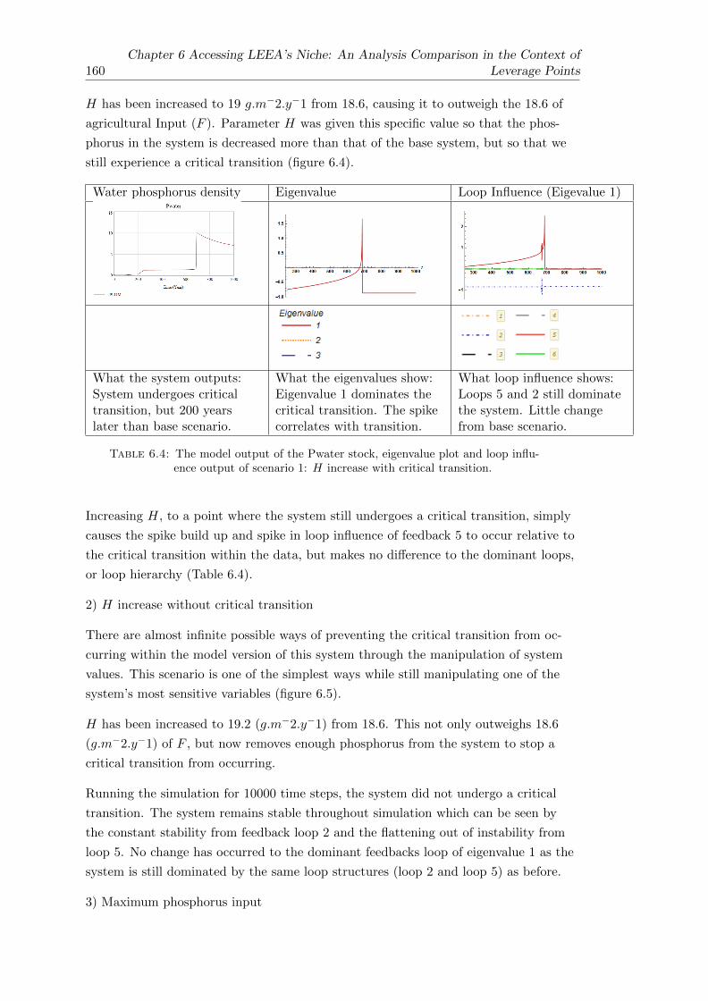
160Chapter 6 Accessing LEEA’s Niche: An Analysis Comparison in the Context of
Leverage Points
H has been increased to 19 g.m−2.y−1 from 18.6, causing it to outweigh the 18.6 of
agricultural Input (F ). Parameter H was given this specific value so that the phos-
phorus in the system is decreased more than that of the base system, but so that we
still experience a critical transition (figure 6.4).
Water phosphorus density Eigenvalue Loop Influence (Eigevalue 1)
What the system outputs:System undergoes criticaltransition, but 200 yearslater than base scenario.
What the eigenvalues show:Eigenvalue 1 dominates thecritical transition. The spikecorrelates with transition.
What loop influence shows:Loops 5 and 2 still dominatethe system. Little changefrom base scenario.
Table 6.4: The model output of the Pwater stock, eigenvalue plot and loop influ-ence output of scenario 1: H increase with critical transition.
Increasing H, to a point where the system still undergoes a critical transition, simply
causes the spike build up and spike in loop influence of feedback 5 to occur relative to
the critical transition within the data, but makes no difference to the dominant loops,
or loop hierarchy (Table 6.4).
2) H increase without critical transition
There are almost infinite possible ways of preventing the critical transition from oc-
curring within the model version of this system through the manipulation of system
values. This scenario is one of the simplest ways while still manipulating one of the
system’s most sensitive variables (figure 6.5).
H has been increased to 19.2 (g.m−2.y−1) from 18.6. This not only outweighs 18.6
(g.m−2.y−1) of F , but now removes enough phosphorus from the system to stop a
critical transition from occurring.
Running the simulation for 10000 time steps, the system did not undergo a critical
transition. The system remains stable throughout simulation which can be seen by
the constant stability from feedback loop 2 and the flattening out of instability from
loop 5. No change has occurred to the dominant feedbacks loop of eigenvalue 1 as the
system is still dominated by the same loop structures (loop 2 and loop 5) as before.
3) Maximum phosphorus input

Chapter 6 Accessing LEEA’s Niche: An Analysis Comparison in the Context ofLeverage Points 161
Water phosphorus density Eigenvalue Loop Influence (Eigevalue 1)
System no longer undergoesa critical transition.
All eigenvalues either 0 ornegative showing a stablesystem, Eigenvalue 1 domi-nates.
Loops 5 and 2 still dominatethe system. Relative influ-ence values of the loops heav-ily decreased with respect toother loops.
Table 6.5: The model output of the Pwater stock, eigenvalue plot and loop influ-ence output of scenario 2: H increase without critical transition.
This scenario consisted of decreasing parameter H and increasing F to provoke an
early critical transition and to maximise phosphorus input to the system (figure 6.6).
H and F were identfied by SA as two parameters in the system with the highest de-
grees of general sensitivity. Phosphorus input was increased to its maximum possible
within the system, while maintaining within the values of Carpenter (2005) by increas-
ing F to 31.6, and reducing H to 0.
Water phosphorus density Eigenvalue Loop Influence (Eigevalue 1)
System undergoes a criticaltransition early then rapidlyincreases with time.
Eig. 1 dominates, spike cor-relates with transition.
Loop 5 dominates the tip,loop 2 dominates the sta-bility within the system inalternative state.
Table 6.6: The model output of the Pwater stock, eigenvalue plot and loop influ-ence output of scenario 3: Maximum phosphorus output.
The simulation makes the critical transition of the lake happen almost immediately,
but makes no change to the loop hierarchy (Table 6.6). It appears that so long as a
critical transition occurs within the system, loop 5 will always dominate the system in
accordance to this transition.
4) Purposeful reduction in loop influence
This scenario manipulates five of the most impactful factors identified within DDWA
leading up to the forward critical transition. Three of the parameters chosen (m, r

162Chapter 6 Accessing LEEA’s Niche: An Analysis Comparison in the Context of
Leverage Points
and q) are directly connected to the system’s most impactful positive feedback loop
(loop 5, concerning phosphorus recycling of the lake sediment). Parameter values of
m, c, q, b and r have been manipulated in a direct attempt to change the loop hierar-
chy within the system’s dominant eigenvalue (see table 6.7). The scenario was imple-
mented by reducing parameters directly linked to loop 5 and increasing parameter b,
which is linked to two stabilizing (negative feedback) loops, 1 and 4.
Water phosphorus density Eigenvalue Loop Influence (Eigevalue 1)
System initially overshoots,reduces then recovers.
Eig 1 still the dominanteigenvalue but heavily re-duced with respect to othereigenvalues.
Loops 5 and 2 still domi-nate this behaviour mode,but their influence is heavilyreduced compared to otherloops.
Table 6.7: The model output of the Pwater stock, eigenvalue plot and loop influ-ence output of scenario 4: Purposeful reduction in loop influence.
With this change all eigenvalues are negative showing that the system is heavily damp-
ened. Of note, eigenvalue 1 is not as prevalent within the system as in other scenarios,
but still holds dominance over the system.
From loop influence plot within Eigenvalue 1 (table 6.7) we can see that despite the
change shown within the loop gain plot, there has been little change in the loop order
of loop influence within the dominant eigenvalue. The influence of loops 2 and 5 have
decreased with respect to the other loops, but they still dominate the stability and
instability generated within this mode.
This scenario has been partially successful in reducing the influence of loops 2 and 5
within the system. The reduction in loop influence was achieved through the manipu-
lation of their directly connected parameters. However, to achieve this outcome, vari-
ables in question had to be manipulated to an unrealistic extent, where values associ-
ated within the most influential loops were dropped to only 10% of their base model
values which is unrealistic for the real world system. The difference made with regard
to influential loop structures and influence hierarchy is minimal as the most influential
loops within the dominant mode remain to be loops 2 and 5.
Despite this deliberate attempt to manipulate the hierarchy of feedback loop influence
within the system, loops 2 and 5 still dominate over the system in all four scenarios.
The main difference between each scenario is how dominant the loops appear with
respect to other loops and whether their influence increases or decreases over time.

Chapter 6 Accessing LEEA’s Niche: An Analysis Comparison in the Context ofLeverage Points 163
While the results of this test cannot be extrapolated to infer anything of other ecosys-
tem models, it has shown within this model how prevalent the influential dynamics are
within the system and how they continue to dominate as key dynamical mechanisms,
despite deliberate parameter manipulation.
6.6 Discussion
Reflecting on the analysis techniques
Parameters H and F are identified by SA which the system was most sensitive to, yet
they are not directly connected to the most influential loops in the system. This infers
that there is a disconnect between the most influential loop structures and individual
parameters the system is most senistive to. This disconnect between the two analy-
sis techniques has occurred for the following two reasons 1) Local sensitivity analysis
(one-at-a-time approach) is not able to account for the dynamics that occur within the
model. 2) Loop analysis is unable to account for sections of the model which are not
defined by loop structures.
Despite their different results, these methods are not necessarily in disagreement as
to the most important and influential parts of the system. It is important to distin-
guish the difference between parameters which the system is highly sensitive to and
the dynamics which are most influential over the system’s behaviour because these
two things are evidently different.
Feedback loops are responsible for the behaviour that we see in the model. So dom-
inant feedback within the system determines which behaviours we can expect to get
out of the system. Parameters which the system is the most sensitive to determine the
extent to which we see that behaviour being expressed and at what point in time we
see it occurring within the data.
In the PLUM model the presence and dominance of loop 5 is associated with the crit-
ical transition within the system. That is to say that whenever Loop 5 becomes dom-
inant, the system experiences a critical transition as that is the dynamic behaviour
associated with the dominance of that loop. When and if loop 5 becomes dominant is
heavily determined by the initial conditions of the system.
Reflecting on the system’s dominant loop structures
Regarding the four scenarios explored by conducting sensitivity tests on LEEA’s out-
put, it would appear that no matter how much the system’s most sensitive variables
are tweaked to avoid the critical transition dynamic or impede the dominance of the
main two loops, the same two loops remain as highly influential structures regardless.

164Chapter 6 Accessing LEEA’s Niche: An Analysis Comparison in the Context of
Leverage Points
This raises interesting questions regarding the relationship between critical transition
dynamics and feedback structures.
When H is adjusted so that the critical transition no longer occurs, the system re-
mains stable in its original state and the same stabilising loop (loop 2) dominates
throughout the entire simulation. No amount of changing this highly sensitive param-
eter within the bounds of +/-10% affects the hierarchy of loops which dominate the
system’s dynamics.
It seems that so long as the critical transition occurs at some point within the simu-
lation, loop 5 will spike relative to that transition, otherwise loop 2 keeps the system
stable. In scenarios generated where the critical transition is unable to occur, regard-
less of parameter manipulation, loop 2 will always dominate the system’s stability. It
could be that within this model, there are simply not enough dynamics to compete
with the influence of loop 2’s negative feedback or loop 5’s positive feedback during a
transition.
A major question therefore is, does it take an entirely new behavioural dynamic within
the system to be expressed before different loops come into play? Intuitively the an-
swer is yes, so long as the same loops always dominate, the same dynamics will always
be expressed within the system. However, we can see from scenario 2 that this is not
inherently true, as feedback loop 5 is the second most dominant feedback loop within
the system, but its influence plateaus, rather than grows exponentially, meaning that
the system never experiences a critical transition. This means that not only the build-
up of influence is important to recognise within these systems, but the trajectory by
which it does so. In the case of PLUM, exponential build-up of loop 5’s influence leads
to a critical transition within the system, but a plateauing trajectory means the condi-
tions for a critical transition are never achieved because the instability of loop 5, never
overtakes the stability of feedback loop 2.
One of the advantages that LEEA holds over Sensitivity Analysis is its ability to dis-
play the change of loop influence through time. When interpreting a loop influence
plot from LEEA, any point may be chosen along a time series and a hierarchy of loop
influence may be determined. Sensitivity analysis, particularly local SA, tends to at-
tribute a single value to each tested variable, its sensitivity degree, which represents
the system’s sensitivity to that variable for the whole simulation meaning the impor-
tance of a variable is assumed to be uniform across an entire simulation. This occurs
because the interactions between the variables (and therefore the dynamic properties)
within the system are not accounted for at a local level.
LEEA allows the user to provide good explanations of system-wide behaviour, with
DDWA allowing the user to infer the causes of stock behaviour from individual links
and parameters contained within loop systems. However, the interpretation of poten-
tial leverage points in this manner can run into difficulties. Suppose a scenario where

Chapter 6 Accessing LEEA’s Niche: An Analysis Comparison in the Context ofLeverage Points 165
LEEA has identified two highly influential loops within a system, one generating high
instability in the system and one high stability. Now suppose that these two loops
share a link as part of their chains. LEEA may allow you to conclude that this link
is a major factor in the behaviour of this system, but it is undermined by the extent
to which inducing a change within this link will impact either loop. This scenario can
be seen occurring within a model system from Saleh et al. (2010).
Implications for leverage point identification and connection to policy
With a dominant driving structure over a system’s behaviour known, it is valuable
to understand what control is held over that structure for conservation, manipulation
and recovery purposes. Extrapolating this knowledge to possibilities for manipulating
a target system via manipulation of its feedback loops, it might be tempting to con-
clude that manipulation of the most dominant feedback loop is the answer to steering
the target system. There are however, multiple caveats within this line of thought;
1. The interconnected nature at which feedback loops occur means that feedback
loops are seldom capable of changing independently and the manipulation of one
will cause change to others (luckily this is why we have model simulation.)
2. When a loop displays as dominant over a target system, it is not easy to de-
termine through LEEA alone, how sensitive the dominance of that loop is to
changes within the individual parameters of the system. This is important with
regards to loop manipulation.
3. With the resources and physical ability to influence the system, it must be ap-
preciated that it may not always be possible to affect any of the components
that are integrated within the most dominant feedback loop. Solutions for in-
voking change on the target system would therefore have to be achieved by con-
sidering alternative feedback loops or variables with less dominant influences.
4. It is possible that the manipulation of a system’s dominant feedback loop would
never result in the desired change to the system’s behaviour because the dy-
namics inherent in that feedback prevent the desired behaviour from ever being
achieved within our physical or economic capabilities. It may be that the only
way to generate positive and effective change within a system is to totally re-
move that feedback loop from the system.
It is false to assume that we could strengthen or weaken the impact of a specific loop
by altering the parameter values directly linked to those loops. This has profound
implications regarding leverage point identification and feedback loop manipulation;
namely finding the system’s most dominant feedback loop does not go hand in hand
with the identification of a system’s most effective leverage points.

166Chapter 6 Accessing LEEA’s Niche: An Analysis Comparison in the Context of
Leverage Points
Relating this to policy, suppose that the goal of system management is making sure
that that critical transition never happens on another lake system, similar to the one
simulated within PLUM. Leverage points from this system can come from two angles
A) focus on the parameters which the system is most sensitive to (i.e. in this case in-
creasing H or reducing F ) or B) focus on altering the system in such a way that an-
other, stabilizing feedback loop becomes dominant.
A) Assumes that the dominance and hierarchy of feedback loops and therefore dy-
namic properties of the system are inevitable or too difficult to change. B) Assumes
that changing the most sensitive parameters in the systems is not going to make any
difference because the system will inevitably undergo the behaviour anyway. A) Is
theoretically easier to do because you are only having to affect one parameter B) May
take more work, but in the end will yield a much better result as you have prevented
the dynamics responsible for the undesirable behaviour from dominating within the
system.
An example of this difference can be explained using real life examples of attempts to
recover lake systems from eutrophic states back to clear conditions.
In Lake Erhai China, (Guo et al. 2001) one of the practices imposed to try and restore
the lake from its eutrophic transition was to restrict the amount of runoff nutrients
entering the water system. This is equivalent to policy scenario A and reducing pa-
rameter F within the system.
In Lake Trehrningen, Sweden (Annadotter et al. 1999; Ryding 1982) the practice im-
posed was to dredge the lake of all of its high phosphorus sediment, thus removing the
mechanism of phosphorus recycling from the lake and stopping the dynamics main-
taining high levels of phosphorus in the system. This is equivalent to policy scenario B
and changing the hierarchy of feedback loops so that the loop 5 would no longer domi-
nate the system.
In order to control a system, an important step is to identify which parts of the sys-
tem you can physically impact with regards to physical, ethical and economic con-
straints. This first step can largely be achieved through qualitative research at the
beginning of a project, bringing together agents from all aspects on the system from
those who use it for business, those who rely on it for wellbeing, those who exploit it
for resources etc.
It is also important to acknowledge what the goal of the policy is i.e. what is the be-
haviour/component of the system that you wish to influence. Once these have been
established a comparison can then be made of which parts you are knowingly able to
impact and those that the analysis identifies as influential system components.
If both the influential components of the system and the parts of the system able to
be affected by human intervention are the same, then policies can be built around

Chapter 6 Accessing LEEA’s Niche: An Analysis Comparison in the Context ofLeverage Points 167
the ability to directly affect an influential structure within the system. If the two are
different, then a discussion must arise; can a knock on effect be implemented within
the system whose end goal is to impact an influential structure which is otherwise un-
changeable.
The propagation of error
The sensitivity analysis within this chapter can give some idea of how error associated
with a variable within a system might propagate through the model output and im-
pact the results of LEEA. As this chapter has already shown, a change of +/- 10% of
a variable’s initial conditions can have profound effects on system behaviour. If the
error associated with a variable happened to be a key component of a dominant feed-
back loop, this would filter down through the Jacobian Matrix, into the eigenvalues
and could completely change where a feedback loop registers within the influence plot.
Although not directly addressed within this thesis, a useful study would be to investi-
gate how error associated with model variables could propagate through the analysis
process.
6.7 Conclusion
This study examines Loop Eigenvalue Elasticity Analysis (LEEA) in the context of
identifying system leverage points and questions whether LEEA on its own is substan-
tial enough to identify system leverage points to the extent where policy decision mak-
ing and implementation can be based of the results. LEEA is also compared along-
side sensitivity analysis, a technique commonly used to identify key drivers of system
behaviour. The results highlight the importance of considering our ability to manip-
ulate different parts of a system. The manipulation of a dominant feedback loop may
prove more of a challenge than a single variable within that loop. The results of the
chapter also highlight that analyses can produce different outputs of which variables
are considered the key drivers, depending on whether they are analysed as individual
variables or as part of feedback structures and this has consequences for the way we
might address which parts of a system to target in policy. Loop Eigenvalue Elasticity
Analysis might be exactly the right tool needed for the identification of leverage points
within complex dynamic systems.

168Chapter 6 Accessing LEEA’s Niche: An Analysis Comparison in the Context of
Leverage Points
Chapter 7: Chapter Preface
LEEA has now been successfully applied and tested on a model system of a shallow
lake, alongside exploring its limitations and potential utility in identifying system
leverage points. While the application of LEEA has proved it can be applicable to dy-
namics of lake hysteresis, it is important to explore the analysis in other socio-ecological
contexts, if for no other reason than to show this analysis is not just applicable to lake
ecology.
In the next chapter, LEEA is applied to an alternative socio-ecological system con-
cerning the mono vs. bistability of coral reef systems. Not only does this chapter eval-
uate LEEA on an entirely different model system, it shows that LEEA can be used
to great effect with an entirely different agenda of the model. In the PLUM model,
LEEA was used to explore which feedback loops are dominating a critical transition,
but in this chapter, LEEA is used to investigate the difference in the role of feedback
loops in a monostable coral reef vs. a bistable coral reef.

Chapter 7
LEEA’s Application to a Coral
Reef System Capable of
Alternative States - Multiple
Feedback Analysis
7.1 Abstract
Coral reef degradation caused by anthropogenic activities is a major issue to coral
reef biodiversity and ecosystem services worldwide. Major species of the reef includ-
ing coral, macroalgae and herbivores are influenced by feedback mechanisms that act
within and between the ecological and social spheres. Understanding these feedbacks,
how and where they operate and the extent to which they drive and control the state
of the reef has an important role in controlling and preventing ecosystem collapse,
while reinforcing recovery. It is unconfirmed through empirical evidence whether hys-
teresis and alternative stable states exist within coral reef systems (as they have been
proven to in shallow lakes), but it is important that we study and understand these
phenomena within reef systems, as they have implications on reef restoration and ma-
rine conservation.
This study develops the analysis of a theoretical coral reef model. The model was
originally created to explore how hysteresis might be generated in a reef system as
a consequence of multiple feedback mechanisms reinforcing one another’s behaviour.
The extension conducts structural analysis on the model system, quantifying the influ-
ence which each feedback loop has over the system’s behaviour at times of mono and
bistability. The purpose is to explore how the study of feedback loops within ecosys-
tems may be extended and used on reef models in the future to help us understand
169

170Chapter 7 LEEA’s Application to a Coral Reef System Capable of Alternative States -
Multiple Feedback Analysis
endogenous system drivers and interpret their impact on system behaviour. The re-
sults of this study show that the feedback structures responsible for generating hys-
teresis within the system do not have a high level of impact directly to the system’s
behaviour, but instead amplify the contribution which every other feedback loop in
the system produces. System hysteresis is shown to be generated through the amplifi-
cation of every feedback loop within the system, rather than a small set of loops which
dominate the system’s behaviour.

Chapter 7 LEEA’s Application to a Coral Reef System Capable of Alternative States -Multiple Feedback Analysis 171
7.2 Introduction
Coral reef degradation has become a large threat to the biodiversity and ecosystem
services which coral reefs are able to provide. Pollution, nutrient loading, overfishing
and poor boating practices are just some of the anthropogenic drivers which act to
harm the reef ecosystem (Zaneveld et al. 2016). The practice of coral reef conservation
is concerned with large system drivers on both short (nutrient and sediment loads)
and long (climate change) timescales. Coral reefs can come under threat from multiple
sources simultaneously, where system recovery can become impossible as previous sta-
ble attractors cease to exist and fast adaption into new niches becomes the only hope.
In order to protect, conserve and restore coral reefs, it is important for us to know the
extent to which human activities can drive these systems away from coral rich states
and how we can focus our efforts should the reefs undergo undesirable regime shifts to
conditions where the corals and fish species are not able to thrive.
A major concern for reef systems is whether they are capable of hysteresis, undergo-
ing critical transitions between coral-dominanted and macro-dominanted stable states.
Despite a lack of empirical evidence for alternative stable states being present within
reef systems, alternative stable states have been observed within other ecosystems
(Hughes et al. 2003, Scheffer and Carpenter 2003, Scheffer and Jeppesen 1998) and
their potential presence has profound implications for coral reef restoration. Investi-
gating the potential existence of alternative stable states has importance, not only for
current theories of coral reef states, reef maintenance and recovery, but also on the
capabilities of future models. We cannot predict a future transition within a model
simulation, if the dynamics are not present in the model to allow it to happen.
Van de Leemput et al. (2016) investigates how hysteresis and therefore alternative sta-
ble states can be generated within a model coral reef system when feedback mecha-
nisms, which individually hold negligible effect over the system, combine to reinforce
each other’s behaviour. Whether real world coral reefs are capable of hysteresis is vital
to understand with regards to system stability, system recovery and species conser-
vation (Scheffer 2009, Knowlton and Jackson 2008). Feedback loops play a vital role
within system stability where negative feedbacks act to maintain a system within a
stable equilibrium and positive feedbacks act to drive systems out of stable equilibri-
ums.
Van de Leemput et al. (2016) model dynamics within a generalised coral reef system
to investigate potential causes or drivers of alternative stable states being present.
The dynamics within their model focus on three main community groups which act
upon the reef: corals, macroalgae and herbivores. The dynamics present the co-operation
and competition that occurs between the three groups. Alternative stable states are
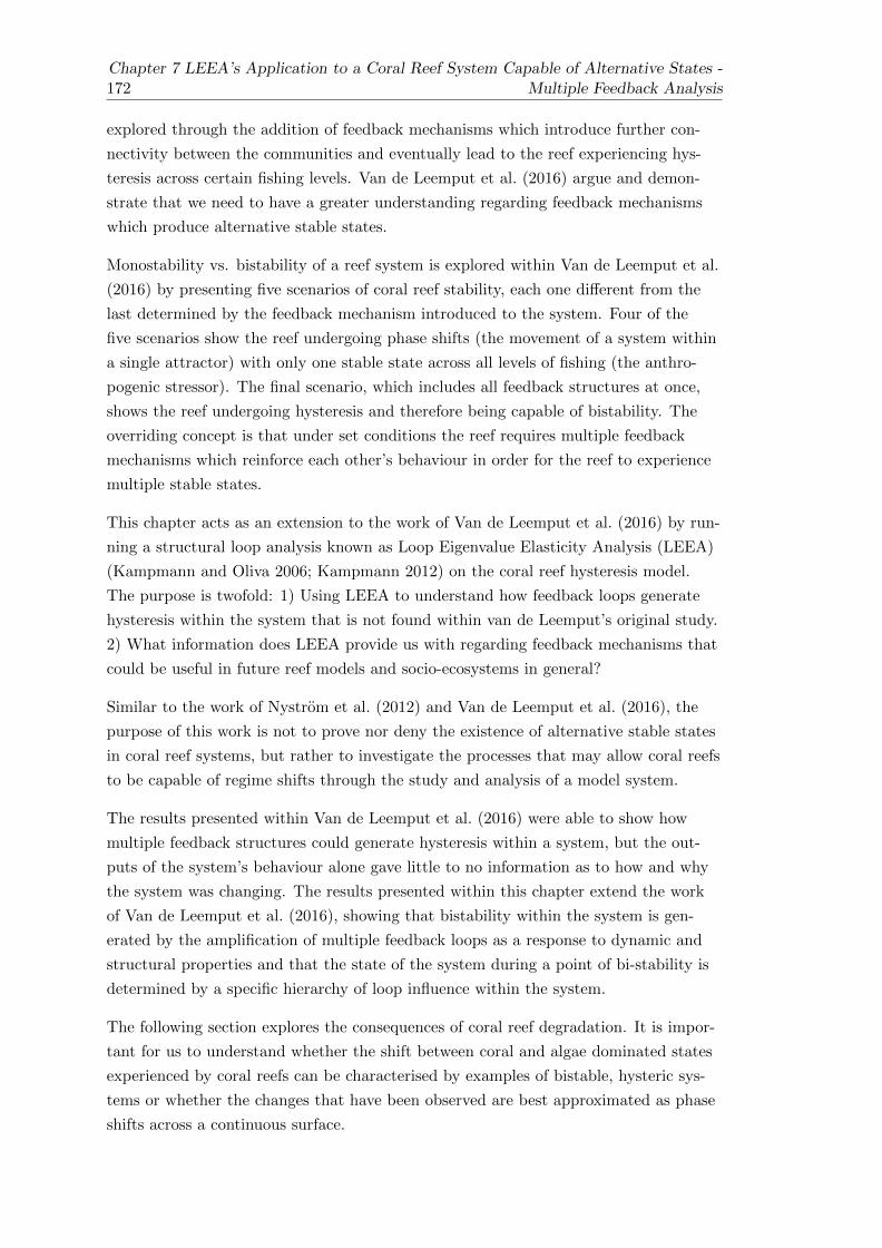
172Chapter 7 LEEA’s Application to a Coral Reef System Capable of Alternative States -
Multiple Feedback Analysis
explored through the addition of feedback mechanisms which introduce further con-
nectivity between the communities and eventually lead to the reef experiencing hys-
teresis across certain fishing levels. Van de Leemput et al. (2016) argue and demon-
strate that we need to have a greater understanding regarding feedback mechanisms
which produce alternative stable states.
Monostability vs. bistability of a reef system is explored within Van de Leemput et al.
(2016) by presenting five scenarios of coral reef stability, each one different from the
last determined by the feedback mechanism introduced to the system. Four of the
five scenarios show the reef undergoing phase shifts (the movement of a system within
a single attractor) with only one stable state across all levels of fishing (the anthro-
pogenic stressor). The final scenario, which includes all feedback structures at once,
shows the reef undergoing hysteresis and therefore being capable of bistability. The
overriding concept is that under set conditions the reef requires multiple feedback
mechanisms which reinforce each other’s behaviour in order for the reef to experience
multiple stable states.
This chapter acts as an extension to the work of Van de Leemput et al. (2016) by run-
ning a structural loop analysis known as Loop Eigenvalue Elasticity Analysis (LEEA)
(Kampmann and Oliva 2006; Kampmann 2012) on the coral reef hysteresis model.
The purpose is twofold: 1) Using LEEA to understand how feedback loops generate
hysteresis within the system that is not found within van de Leemput’s original study.
2) What information does LEEA provide us with regarding feedback mechanisms that
could be useful in future reef models and socio-ecosystems in general?
Similar to the work of Nystrom et al. (2012) and Van de Leemput et al. (2016), the
purpose of this work is not to prove nor deny the existence of alternative stable states
in coral reef systems, but rather to investigate the processes that may allow coral reefs
to be capable of regime shifts through the study and analysis of a model system.
The results presented within Van de Leemput et al. (2016) were able to show how
multiple feedback structures could generate hysteresis within a system, but the out-
puts of the system’s behaviour alone gave little to no information as to how and why
the system was changing. The results presented within this chapter extend the work
of Van de Leemput et al. (2016), showing that bistability within the system is gen-
erated by the amplification of multiple feedback loops as a response to dynamic and
structural properties and that the state of the system during a point of bi-stability is
determined by a specific hierarchy of loop influence within the system.
The following section explores the consequences of coral reef degradation. It is impor-
tant for us to understand whether the shift between coral and algae dominated states
experienced by coral reefs can be characterised by examples of bistable, hysteric sys-
tems or whether the changes that have been observed are best approximated as phase
shifts across a continuous surface.

Chapter 7 LEEA’s Application to a Coral Reef System Capable of Alternative States -Multiple Feedback Analysis 173
Ecosystems which have previously been recorded degrading due to anthropogenic ac-
tivity have been shown capable of transitioning between alternative stable states (ex-
pressing hysteresis), driven by positive feedback loops. The clearest examples of this
from both empirical data and dynamic modelling practices can be seen within shal-
low lake systems (Carpenter et al. 2003; Carpenter 2005; Scheffer 2009). It is debated
across the scientific community, whether the same principles of alternate stable states
exist within coral reef systems, or whether they are single state systems, capable of
dramatic phase shifts away from their single stable state (Knowlton 2004; Norstrom
et al. 2009; Fung et al. 2011).
While it is difficult to determine whether real-world socio-ecosystems are capable of
transitioning between alternative stable states, understanding the potential dynam-
ics is of upmost importance affecting system management. Systems which transition
between alternative stable states are difficult to reverse due to the nature of hysteresis.
7.3 Background
Coral reef degradation
Coral reefs provide goods and services to societies worldwide through seafood, re-
source consumption, recreational activity, tourism, culture and coastal protection (Pauly
et al. 2005; Daily 1997). While they only occupy roughly 0.1-0.5% of the sea floor,
they account for one third on the ocean’s fish species (Moberg and Folke 1999), mak-
ing them a key support mechanism for marine biodiversity.
Ecosystem degradation has been shown in coral reefs (Nystrom et al. 2012), grass-
lands (Ravi et al. 2010) and shallow lakes (Scheffer 2009). Ecosystem degradation is
the deterioration of the environment through depletion of resources, the destruction of
ecosystems, habitat, extinction of wildlife and pollution (Johnson et al. 1997). When a
coral reef is degraded, its ecosystem services are reduced (Nystrom et al. 2012).
“Coral reefs are major reservoirs of biodiversity and render goods and services that
support the livelihoods of millions of people worldwide, but are being degraded rapidly.”
(Fung et al. 2011).
Globally it has been near impossible to find a reef that has been and remains unaf-
fected by human activity (Hughes et al. 2003, Halpern et al. 2008). As anthropogenic
activity surrounding the reefs increase, knock on effects occur to the quality and quan-
tity of the reef’s good and services (Moberg and Folke 1999). Examples of coral reef
net worth include coastal protection, valued between $820-1 000 000 per km coastline
in Indonesia (Cesar 1996), waste assimilation services at $58 per hectare per year in
the Galapagos (De Groot et al. 1992) and the financial value of tourism estimated at
$8 900 000 000 in the 1990s over the Caribbean (Dixon et al. 1993). Overfishing, coral

174Chapter 7 LEEA’s Application to a Coral Reef System Capable of Alternative States -
Multiple Feedback Analysis
bleaching, runoff of nutrients and sediment from industrial activity, pollution, disease,
dynamite fishing, cyanide fishing, use of coral as building materials and climate change
have all been observed having adverse effects on the wellbeing of a reef (Wagner 1997;
Jones and Hoegh-Guldberg 1999; Knowlton 2001; Hughes et al. 2003; Syvitski et al.
2005; Hoegh-Guldberg et al. 2007). These factors have all been shown to degrade the
system causing decline in the species abundance, resilience and habitat structure.
Hysteresis and feedback dynamics
Hughes et al. (2010) express that while scientific effort surrounding coral reefs has
concentrated on shifts into degraded states, less focus has been directed to the mecha-
nisms (incl. feedback dynamics) which cause them and prevent or impair their recov-
ery. The role of feedback loops as driving mechanisms within ecosystems should be a
key subject of study regardless of whether coral reefs are capable of alternative stable
states or not. Positive feedback loops not only drive transitions between states, but
also retard the recovery of systems driven out of single stable states, both of which
are costly to social and ecological spheres (Knowlton 2004). Studies of coral reefs
which concentrate on the role of feedback dynamics have also seen use in decision sup-
port systems concerning coastal management programmes and practices (Chang et al.
2008).
The debate of alternative states vs. phase shifts has importance from a system re-
covery perspective and within the context of marine conservation biology (Knowl-
ton 2004). Degradation of coral reefs generally lead them to becoming algal domi-
nated; if alternative stable states exist within the system, then our ability to restore
the reefs to coral dominance is hindered by the properties of hysteresis (lags in recov-
ery) caused by ecological feedbacks which reinforce the algae dominant state (Nystrom
et al. 2012).
“Reversal of environmental conditions to levels close to that which precipitated a de-
graded stable state will not lead to a recovery, these circumstances pose a particular
challenge for managers” (Fung et al. 2011).
Nystrom et al. (2012) suggest that it may be a shift in driving ecological processes
that lock a system into an alternative degraded state. In theory, a phase shift is easier
to reverse (Beisner et al. 2003). However, even phase shifts can be difficult to reverse
if they are driven by large, persistent environmental changes such as toxic chemical
spills (Mumby 2009, Dudgeon et al. 2010).
It is much better to avoid undesirable state transitions as they can be difficult to re-
verse with increasing difficulty as the system degrades (Suding et al. 2004, Suding and
Hobbs 2009)
How can understanding feedback loops help us with hysteresis?

Chapter 7 LEEA’s Application to a Coral Reef System Capable of Alternative States -Multiple Feedback Analysis 175
In their study of feedbacks within degraded marine ecosystems, Nystrom et al. (2012)
introduce three concepts of feedbacks which we need to understand better in order to
seek successful management of marine ecosystems:
1. The way human actions influence the strength and direction of feedbacks.
2. How different feedbacks interact.
3. The scales at which feedbacks operate.
Nystrom et al. (2012) approach these concepts by investigating the extent to which
critical feedbacks are represented within current management practices of degraded
marine systems. Their work involves description and illustration of complex feedback
synergies, real world examples and speculation on how to conduct feedback breaking
through policy and management, but the analysis of the feedback mechanisms is taken
no further. In this study, the work from Van de Leemput et al. (2016) is extended to
show how LEEA, may help us to qualitatively and quantitatively gain a greater un-
derstanding of how feedback mechanisms hold influence within a coral reef model and
in doing so, better understand points 1, 2 and potentially 3 of Nystrom’s introductory
requirements for successful management practices.
While there are many different approaches to investigating and testing Nystrom’s
three points, this study approaches them through the following: 1) is investigated by
the manipulation of the major social variable within the model (fishing) to see how
feedback mechanisms within the system are affected over its range of values. 2) is in-
vestigated by analysing how feedback loops are affected by the presence or absence
of other loops. 3) is more difficult to investigate within this study as we only investi-
gate one model where the feedbacks are set to act only within and between three main
species of the reef.
Nystrom et al. (2012) states that the purpose of studying these three points is to un-
derstand how and when we can influence these feedback mechanisms (What window of
opportunity do we have?) in order to reduce the resilience of a degraded system. Ex-
panding on this, better understanding of critical feedback processes may also allow us
to increase and/or maintain the resilience of a preferred system state.
Alternative stable states in coral reef systems
Van de Leemput et al. (2016) investigate feedback loops within a reef system able to
experience hysteresis (Scheffer et al. 2001) and therefore containing alternative sta-
ble states. This stems from an ongoing debate within the academic community as to
whether or not coral reefs are capable of alternative stable states.
Coral reefs are capable of being dominated by either coral cover, or algae cover as the
two compete for space on the reef. The debate is whether transitions between these

176Chapter 7 LEEA’s Application to a Coral Reef System Capable of Alternative States -
Multiple Feedback Analysis
two conditions occur as phase shifts within a system which has only one stable attrac-
tor, or as alternative stable states within a system that contains two (or more) stable
attractors.
It is important to study and test alternative stable states numerically within system
models as they can be difficult to test for in the real-world (Scheffer and Carpenter
2003). Mumby et al. (2013) discuss three reasons why alternative states can be diffi-
cult to test for within a real-world reef system: 1) In coral reef systems, the dynamics
associated with corals occur slowly over year to decade timescales (Adjeroud et al.
2009; Halford et al. 2004). 2) Stable states are difficult to observe naturally as the
reefs are frequently disturbed by stochastic perturbations i.e. cyclones (Hughes and
Connell 1999). 3) Manipulation of reefs for the purpose of study would be largely pro-
hibited, mainly due to the amount of anthropogenic impact already present across
many reef systems (Petraitis and Dudgeon 2004). Some authors use the second point
to argue against alternative attractors, finding that corals or macroalgal dominant
states rarely exist in the real world (Bruno et al. 2009).
While a coral reef maintaining a non-coral dominant species may be indicative of a
transition into an alternative state, the success of the new species could also be caused
by the imprint of a catastrophic disturbance persisting within the system, changing
and maintaining the ecological community without shifting it into an alternative state
(Dudgeon et al. 2010). Alongside this, some reefs are naturally algal dominated: Vroom
et al. (2006) explore 94 algal dominated reefs in the Central Pacific that are largely
undisturbed by humans. Overall, the frequency of naturally algal dominated reefs
worldwide is unclear (Fung et al. 2011).
Evidence for coral reefs experiencing multiple attractors is discussed within Scheffer
and Carpenter (2003) and Mumby et al. (2013) with the use of field data, statisti-
cal models driven by field data and mechanistic ecological models. As Mumby et al.
(2013) notes, one advantage of simulation models is that a system’s ecology does not
have to be simplified to achieve analytical tractability and alternative attractors can
become emergent properties without conscious implementation.
Fung et al. (2011) found that in their model, critical transitions only occurred when
parameters were set to the extremes of their empirically determined values. Fung
et al. (2011) also discussed that even if reefs were capable of critical transitions, smooth
phase shifts were much more likely within realistic model parameter ranges of reef sys-
tems.
Alternative studies of coral reef transitions focus on stressors that alone or in combi-
nation generate phase shifts or critical transitions between coral and algal dominance
(Van de Leemput et al. 2016; Fung et al. 2011). Fung et al. (2011) discuss how it is
usually difficult to separate the effects of each individual stressor in order to determine
their impact on a phase shift.

Chapter 7 LEEA’s Application to a Coral Reef System Capable of Alternative States -Multiple Feedback Analysis 177
These stressors often include anthropogenic factors which affect the reef, including
overfishing, the aquarium trade, nutrification and sedimentation, as these external
factors bring stresses to the reef that are often the cause of top-down changes from
coral to macroalgae dominated systems (Norstrom et al. 2009). The anthropogenic
factors are also stressors which policy and reef management practices could poten-
tially have the most impact over, as they are largely driven by societal and economic
pressures. In modelling practices, anthropogenic parameters are usually modelled in-
directly through their effects on the ecological processes of the reef, i.e. Fung et al.
(2011) model fishing as a decrease in herbivore biomass.
For their approach, Van de Leemput et al. (2016) construct a mechanistic model to
explore a reef’s ability to contain alternative stable states and the role of feedback
mechanisms in the transitions between those states. Van de Leemput et al. (2016) fo-
cus on fishing as a controlling parameter for their simulation as this has a direct im-
pact on the herbivore population, in turn creating knock-on effects to the death rate
of the algal and coral communities.
7.4 Methodology
Van de Leemput’s Five Coral Reef Scenarios
Van de Leemput et al. (2016) explore the potential for coral reef hysteresis through
the manipulation of system structure and the change in fishing pressures upon the
reef across a series of five scenarios. The five scenarios which they generate can be
identified by the feedback mechanisms that are included within the model structure.
Van de Leemput et al. (2016) show that at any level of fishing pressure, the first four
scenarios of the system are only able to express monostability, having one stable state.
However, under the same initial conditions as set in the first four scenarios, the feed-
back mechanisms within the fifth scenario when combined, are able to reinforce one
another’s dynamics, generating hysteresis and therefore bistability within the system.
The first scenario (scenario i) constitutes the base model which all scenarios stem
from, portraying basic dynamic mechanisms known to operate within reef systems
including competition for space between coral and macro-algae, predation of macro-
algae by herbivores and fishing of herbivores as an anthropogenic pressure on the sys-
tem. Van de Leemput et al. (2016) then present three new feedback mechanisms which
when implemented individually to the base scenario, provide negligible driving pres-
sures on the system. The three feedbacks are named 1) Herbivory-escape 2) Compe-
tition and 3) Coral-herbivore. When all three feedback mechanisms are included at
once, their combined dynamics cause the system to experience hysteresis, meaning the
system becomes bistable at certain levels of fishing.

178Chapter 7 LEEA’s Application to a Coral Reef System Capable of Alternative States -
Multiple Feedback Analysis
Each scenario is defined through a set of equations determining which feedback mech-
anisms are present. Equations of scenario i, which included unoccupied space on the
reef (S), reef covered by coral (C), reef covered by macroalgae (M) and herbivore abun-
dance (H) take the following form:
S = 1− C −M (7.1)
dM
dt= (iM + bMM)S − gHM (7.2)
dC
dt= (ic + bCC)S − dCC (7.3)
dH
dt= rH(1−H)− fH (7.4)
Despite Van de Leemput et al. (2016) coining the base model the ‘No Feedbacks’ sce-
nario, there are eight feedback loops which are generated by these dynamics and are
responsible for the behaviour that is expressed within the first model system (table
7.1).
Loop No. Parameters and Sequance Feedback type
1 Cover by Coral → Coral Inflow → Cover byCoral
Positive
2 Cover by Coral → Coral Outflow → Cover byCoral
Negative
3 Cover by Macroalgae → Macroalgae Inflow →Cover by Macroalgae
Positive
4 Cover by Macroalgae → Macroalgae Outflow→ Cover by Macroalgae
Negative
5 Herbivore Abundance → Herbivore Inflow →Herbivore Abundance
Positive
6 Herbivore Abundance → Herbivore Outflow →Herbivore Abundance
Negative
7 Cover by Coral → Available space on reef →Coral Inflow → Cover by Coral
Negative
8 Cover by Macroalgae → Available spaceon reef → Macroalgae Inflow → Cover byMacroalgae
Negative
Table 7.1: Lists the eight loop structures within Van de Leemput et al. (2016) basescenario coral reef system
The additional feedback mechanisms introduced within scenarios ii-iv, named Herbivory-
escape feedback, Competition feedback and Coral-herbivore feedback respectively were

Chapter 7 LEEA’s Application to a Coral Reef System Capable of Alternative States -Multiple Feedback Analysis 179
developed by Van de Leemput et al. (2016) based on 20 of the best documented posi-
tive feedbacks known to exist within coral reef systems having been qualitatively dis-
cussed in 60 papers (Van de Leemput et al. 2016 and references therein). Many of
the dynamics of these 60 feedbacks were analysed within Mumby and Steneck (2008),
Mumby (2009) and Nystrom et al. (2012).
Feedback loop from scenario ii) Herbivory-escape
Feedback between macroalgae cover and herbivory rate - a scenario where consump-
tion by herbivores saturates when algae are more abundant. This feedback does not
form a structural loop, but generates a direct influence to the death rate of macroal-
gae). The herbivore-escape feedback affects the system when fishing levels are high as
it decreases the herbivore population to the point where algae consumption saturates.
At low fishing levels, when herbivore population is high, the feedback has little effect
on the system.
Feedback loop from scenario iii) Competition (Interspecific)
The competition feedback generates a negative effect of macroalgae population on
coral recruitment. The feedback causes a direct link to form between macroalgae and
coral, where their interaction is no longer purely intraspecific from competing for space.
Intraspecific competition is where: “species are indirectly affected by each other through
space available” Van de Leemput et al. (2016). Interspecific competition: “proportion
of macroalgae directly inhibits coral growth” Van de Leemput et al. (2016).
Feedback loop from scenario iv) Coral-herbivore
The coral-herbivore feedback introduces a direct reinforcing connection from coral
cover to herbivore births, generating a feedback loop to coral through herbivore graz-
ing of macroalgae. Corals promote herbivore growth through habitat and shelter. The
loop structure connects coral cover to herbivore carrying capacity. By doing so it links
the impact of herbivore population to the rest of the system as part of a feedback, in-
stead of a simple linear input to macroalgae death.
The feedbacks present within scenario ii, iii and iv are manipulations of equations 7.2,
7.3 and 7.4 respectively and take the following dynamical form:
Herbivory-escape feedback:
dM
dt= (iM + bMM)S − gHM
gηM + 1(7.5)
Competition feedback:
dC
dt= (ic + bCC)S(1− αM)− dCC (7.6)

180Chapter 7 LEEA’s Application to a Coral Reef System Capable of Alternative States -
Multiple Feedback Analysis
Coral-herbivore feedback:
dH
dt= rH(1− H
(1− σ) + σC)− fH (7.7)
Scenario v makes use of equations 7.1, 7.5, 7.6 and 7.7, the structures of which can be
seen in table 7.2.
Scenario LoopNo.
Parameters and Sequance Feedback type
Herbivory-escape 4+ Cover by Macroalgae → Macroal-gae Outflow → Cover by Macroal-gae
Negative
Competition 9 Cover by Macroalgae → Coral In-flow → Cover by Coral → Unoccu-pied Space → Macroalgae Birth →Cover by Macroalgae
Positive
Coral-Herbivore 10 Cover by Coral → HerbivoreBirth → Herbivore Abundance→ Macroalgae Death → Cover byMacroalgae → Unoccupied Space→ Coral Birth → Cover by Coral
Negative
All Feedbacks 4+, 9& 10
N/A Mixed
Table 7.2: Lists the feedback loop structures within Van de Leemput et al. (2016)additional scenarios
The meanings and values associated with equations 7.1-7.7 can be seen in table 7.3.
Van de Leemput et al. (2016) show how the feedback mechanisms added to the base
scenarios within scenarios ii-iv appear to generate little change in the ecosystem as
the system always remains monostable across all levels of fishing. Van de Leemput
et al. (2016) then use scenario v, which combines all previous feedback mechanisms
together, to show how these feedback loops must not be dismissed as unimportant as
their collective influence generates hysteresis within the system and therefore generate
profound changes in state potential.
Symbols of the model equations and their corresponding values have all been repli-
cated from Van de Leemput et al. (2016) in order to recreate their model scenarios.
The values for each parameter to determine the stable and unstable system states
were calculated by Van de Leemput et al. (2016) using parameter analyses in Mat-
lab. The values for the base model ( scenario i), were based on two assumptions of the
reef: 1) Coral growth rate is always exceeded by macroalgal growth rate. 2) With fish-
ing set to zero, and therefore herbivore population being at maximum capacity, the
macroalgae consumption rate will always exceed the natural death rate of the corals.

Chapter 7 LEEA’s Application to a Coral Reef System Capable of Alternative States -Multiple Feedback Analysis 181
Symbol Name Value
C Cover by Coral 0-1
M Cover by Macroalgae 0-1
H Herbivore Abundance 0-1
S Unoccupied space 0-1
t Time 0-1
f Fishing pressure 0-1
bC Local expansion of existing adults of coral 0.3
bM Local expansion of existing adults of macroal-gae
0.8
iC External import of propagules of coral 0.05
iM External import of propagules of macroalgae 0.05
dC Mortality of corals 0.1
r Growth rate of herbivores 1
g Grazing rate of herbivores 1
η Macroalgae handling time of herbivores 1
α Proportion of macroalgae involved in directinhibition of corals
0.5
σ Relationship strength between coral cover andherbivore carrying capacity
0.6
Table 7.3: Adapted from Van de Leemput et al. (2016). Expresses the symbols,names and values attributed to construct each of the scenarios
Replication of results from Van de Leemput’s ‘All feedbacks’ Scenario (scenario v),
can be seen in figure 7.1. The parameter space where the system becomes capable
of alternative stable states due to multiple feedbacks generating hysteresis occurs be-
tween 33-51% fishing.
Within each scenario, the level of fishing is able to be set anywhere between 0 and
1. 0 fishing indicates that no fishing takes place and therefore no fish are removed
from the system via fishing within the catchment and 1 refers to 100% of the fish are
caught and therefore removed from the catchment. It is through the fishing variable
that the mono-bistability of scenario v, ‘All feedbacks’, is expressed. In order for a
comparison of LEEA results across the different scenarios, one fishing level must be
chosen.
For the analysis of Van de Leemput’s model scenarios, fishing is set to a constant
value of 0.51, or 51% fishing. This value was chosen from the parameter space as it
is one of the final values within scenario v that lies within the bistable region, meaning
that both the coral dominated and macroalgae dominated states could be compared
against all other scenarios, while also making the system close to the point at which
it transitions to a monostable, macroalgae dominated regime at 52% fishing. At 0.51
fishing, all monostable scenarios, i-iv are coral dominated. In total six scenarios are
presented for feedback analysis and comparison. Of the six scenarios, five are coral
182Chapter 7 LEEA’s Application to a Coral Reef System Capable of Alternative States -
Multiple Feedback Analysis
Figure 7.1: A replication of ‘All feedbacks’ scenario from Van de Leemput et al.(2016). The red line represents cover by coral. The green line represents cover bymacroalgae. The blue line represents abundance of herbivores. The bistable zone
occurs between 33% and 51% fishing.
dominated (scenarios i-v at fishing=51%) and one algae dominated (scenario v alter-
native state at fishing =51%).
Extentions of the five scenarios using LEEA
The work of Van de Leemput has been expanded using Loop Eigenvalue Elasticity
Analysis (LEEA), a method developed to identify the influence which individual feed-
back loops hold over a system’s behaviour (Kampmann and Oliva 2006; Kampmann
2012). LEEA is capable of identifying the most dominant loop mechanisms within a
system. By analysing the loop dominance within Van de Leemput’s coral reef system,
the influence of each loop can be plotted relative to every other loop, effectively quan-
tifying the significance of the mechanisms known to generate hysteresis within the sys-
tem. LEEA is able to identify the impact which each feedback loop has on the system
across its range of stable states.
Subjecting the five scenarios to structural loop analysis, a focus is drawn to the three
feedback mechanisms of scenarios ii, iii and iv to compare the influence of these loops

Chapter 7 LEEA’s Application to a Coral Reef System Capable of Alternative States -Multiple Feedback Analysis 183
when analysed separately with respect to when they are comined in scenario v. The
base scenario was analysed to act as a control for comparison across the other scenar-
ios. When all feedback loops are built into one model they are shown to reinforce each
other’s behaviour. LEEA is used to evaluate how the reinforcing behaviours translate
in terms of feedback influence to the system. e.g. Do the feedback loops reinforce each
other equally, or cause one to become dominant?
Each of the 5 scenarios from Van de Leemput et al. (2016) have been built as a sep-
arate model and analysed under the same conditions, the only variation between sce-
narios is the structural addition of the new feedback loop and its associated variables.
The structure of scenario v, which contains all eight original feedback loops and the
three scenario extensions can be seen in figure 7.2. The additional connections formed
by the new dynamics within equations 7.5, 7.6 and 7.7 are highlighted in red. The
feedback loops created by these new dynamics are changed to dashed lines for scenario
ii, dotted lines for scenario iii and bold lines for scenario iv.
Figure 7.2: Cyclic diagram of Van de Leemput et al. (2016) scenario ‘All feed-backs’ containing all eight loops from the base scenario, labelled 1-8 and the threeextensions which collectively form two new structural loops 9 & 10. Any interactionscontained within the base scenario are represented with blue arrows and any inter-actions from the extension scenarios are represented with red arrows. Loops formedby the implementation of each scenario have their arrows adapted in the followingmanner: Scenario ii) Herbivory-escape - dashed arrows, Scenario iii) Competition -dotted arrows, Scenario iv) Coral-Herbivore - bold arrows. Interactions which areinvolved in more than one scenario are represented by the scenario which they first
appear in.
184Chapter 7 LEEA’s Application to a Coral Reef System Capable of Alternative States -
Multiple Feedback Analysis
The scenarios have been subjected to model spin-up, allowing each simulation to move
towards its stable state at 51% fishing before conducting LEEA. The systems have
been plotted in stable state conditions in order to concentrate on the influence of loop
structures which are maintaining the stable state, and exclude any movement towards
these states which were deemed unnecessary for the comparison. From each scenario,
a hierarchy of feedback loop influence can be calculated. The difference between these
hierarchies can then be compared as different feedback mechanisms are added to the
dynamics of the reef across scenarios i to v.
Each scenario has been modelled to 1800 time steps to show how the stability of the
coral, macroalgae and herbivores remains constant throughout time. While the model
was run for a much longer time (around 10000 time steps), 1800 proved sufficient as a
check as almost all critical transitions occurred within this time period if they were
going to occur at all. Results have been displayed in Figures 7.3a, 7.3b, 7.3c, 7.4a,
7.4b and 7.4c. Loop influence for Eigenvalues 1 and 2 have been displayed as these
consistently show the highest contribution to system stability, by having higher abso-
lute values than eigenvalue 3 while all eigenvalues remain negative throughout each
simulation.
7.5 Results
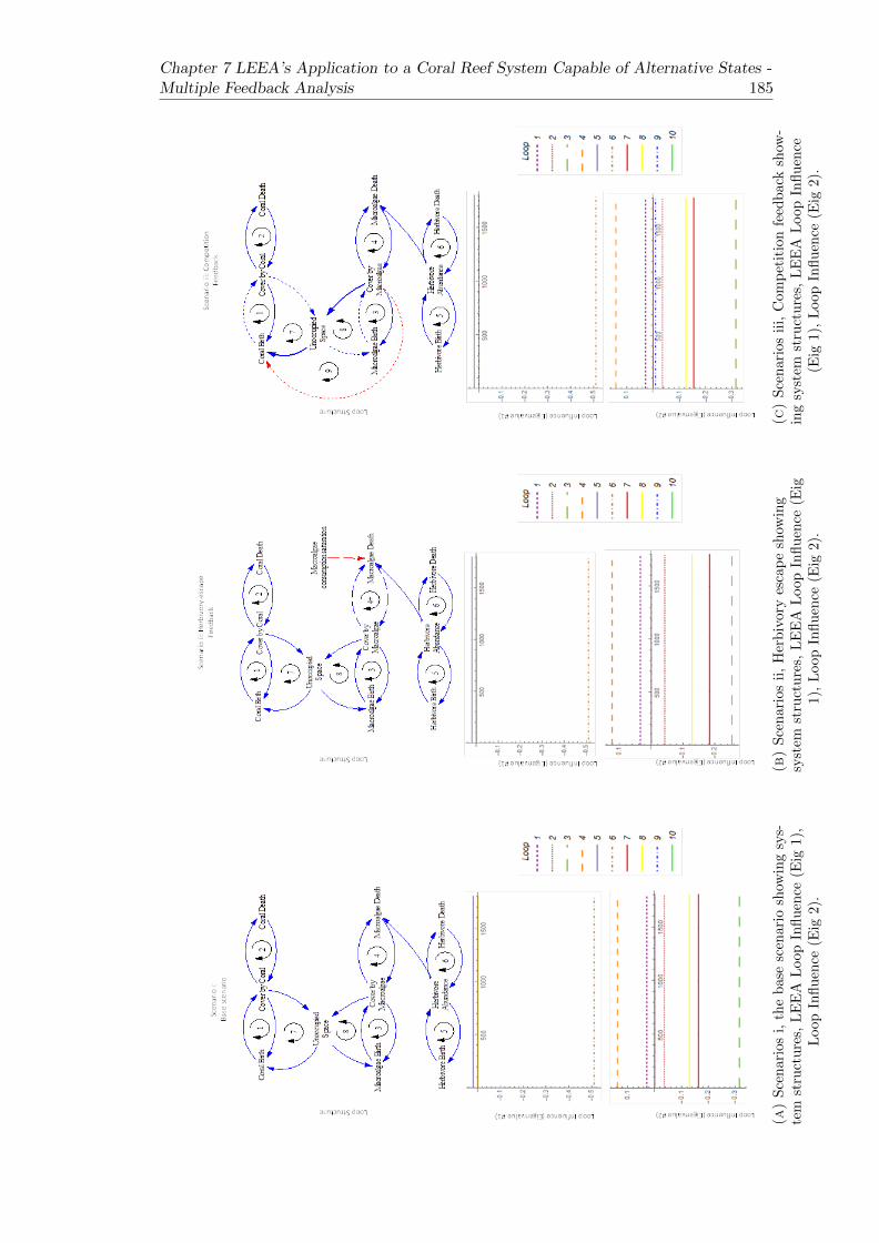
Chapter 7 LEEA’s Application to a Coral Reef System Capable of Alternative States -Multiple Feedback Analysis 185
(a)
Sce
nar
ios
i,th
eb
ase
scen
ario
show
ing
sys-
tem
stru
ctu
res,
LE
EA
Loop
Infl
uen
ce(E
ig1)
,L
oop
Infl
uen
ce(E
ig2)
.
(b)
Sce
nari
os
ii,
Her
biv
ory
esca
pe
show
ing
syst
emst
ruct
ure
s,L
EE
AL
oop
Infl
uen
ce(E
ig1),
Loop
Infl
uen
ce(E
ig2).
(c)
Sce
nari
os
iii,
Com
pet
itio
nfe
edb
ack
show
-in
gsy
stem
stru
ctu
res,
LE
EA
Loop
Infl
uen
ce(E
ig1),
Loop
Infl
uen
ce(E
ig2).

186Chapter 7 LEEA’s Application to a Coral Reef System Capable of Alternative States -
Multiple Feedback Analysis
(a)
Sce
nar
ios
vi,
Cor
al-h
erb
ivor
efe
edb
ack
show
ing
syst
emst
ruct
ure
s,L
EE
AL
oop
Infl
u-
ence
(Eig
1),
Loop
Infl
uen
ce(E
ig2)
.
(b)
Sce
nari
os
v,
All
feed
back
s:co
ral
dom
i-n
ated
show
ing
syst
emst
ruct
ure
s,L
EE
AL
oop
Infl
uen
ce(E
ig1),
Loop
Infl
uen
ce(E
ig2).
(c)
Sce
nari
os
v,
All
feed
back
s:alg
ae
dom
i-n
ate
dsh
owin
gsy
stem
stru
ctu
res,
LE
EA
Loop
Infl
uen
ce(E
ig1),
Loop
Infl
uen
ce(E
ig2).

Chapter 7 LEEA’s Application to a Coral Reef System Capable of Alternative States -Multiple Feedback Analysis 187
The results are displayed in grid format with each column representing a separate
model scenario and each row containing the model structure and loop influence for
eigenvalues 1 and 2. Each of the first four scenarios has one column attributed to it,
while scenario v, ‘All feedbacks’ has two separate states which are analysed separately.
LEEA is calculated where cover by coral, macroalgae and herbivore abundance are
stable with respect to the initial conditions of the auxiliary variables. The stable states
mean that LEEA plots as continuous horizontal lines as the hierarchy of feedback
dominance does not shift when a system rests at equilibrium in this manner.
Structurally, scenario ii, ‘herbivory-escape’ feedback does not generate an extra feed-
back loop within the system, it only acts to reinforce one that is already present which
is why the herbivory-escape feedback is not picked up as a separate structure which
LEEA can identify. In scenario iii, ‘Competition feedback’, the loop structure that
forms is represented by loop 9 (blue dotted line within the models) and in scenario iv,
‘coral-herbivore’, the new feedback mechanism is represented by loop 10 (solid bold
line within the model). Scenario v, ‘All feedbacks contains all the structures com-
bined.
Between sceanrios i-iii, there is not much contrast between the loop influence values.
All systems are dominated by loop 6, which provides stability to the system as its
most dominant negative feedback loop. In terms of populations, in Herbivore-escape
scenario ii, we can already start to see the effect of the 3rd positive feedback mech-
anism creating a decrease in herbivore abundance past the level of fishing which is
occurring in the area. The stable level of herbivore abundance in the three previous
models occurs at 0.49, which reflects that 51% of the fish are removed, leaving 49% to
remain. However, the introduction of the Coral-herbivore loop acts to decrease herbi-
vore levels even further.
From Eigenvalue 1: The presence of the coral-herbivore feedback loop (Loop 10, sce-
nario iv) causes the influence of almost all feedback loops to increase while lowering
the relative influence of loop 6 (herbivore death rate). The impact of fishing has been
reduced relative to other feedback mechanisms.
Structurally, the difference between Coral-Herbivore feedback and All-feedback is the
addition of one feedback loop (loop 9), despite it being the combination of three feed-
back mechanisms. The presence of loop 9 and 10 causes the loop hierarchy of loops 8,
7 and 3 to switch. However, the consequence of these changes is the difference between
the absence and presence of hysteresis within the system.
7.6 Discussion
Detecting the cause of hysteresis

188Chapter 7 LEEA’s Application to a Coral Reef System Capable of Alternative States -
Multiple Feedback Analysis
By analysing each scenario using structural loop analysis through LEEA, the contribu-
tion which each loop has over the system’s behaviour could be compared to each other
loop structure. Thus, whenever a feedback loop was added, generating a new scenario
within the model, LEEA was able to show us exactly how much impact that loop was
generating within the system.
Within each scenario, the individual feedback loops which were added specific to that
scenario showed little to no impact to the system’s output and stability. Across sce-
narios ii to iv, the lack of behavioural change within the system correlates to the low
influence values detected through LEEA. When the addition of a feedback mecha-
nism does not produce a high influence over the system, it may be assumed that the
system’s behaviour would not be affected by the presence of that loop. However, this
study has shown this not to be the case as can be seen and explained through scenario
V: ‘All feedbacks’.
In the results of LEEA for scenario v, the additional feedback structures which are
introduced to the system produce low levels of influence on the system’s behaviour, in-
ferring that these loops have little or no contribution to the system’s output. However,
we know from Van de Leemput et al. (2016) results that it is the addition of these
loops which allow hysteresis within the system to be possible, so what has happened?
While the new feedback mechanisms have little influence over the system’s behaviour
in scenario v, they have profound effects on the other feedback loops present in the
model. This can be seen by comparing the base Scenario i to Scenario v. The main
trigger for the feedback influence hierarchy to change is the coral-herbivore feedback,
producing the greatest change to the base scenario shown by the comparison with Sce-
nario iv. Comparing across loop influence results for Eigenvalue 1, Scenarios i, ii and
iii show only one dominant loop within the system (loop six: herbivore abundance -
herbivore outflow) maintaining the system’s stability. As soon as coral-herbivore feed-
back is introduced within scenario iv, all of the original eight feedback loops increase
to higher levels of influence relative to their influence within the base scenario.
We know from Van de Leemput et al. (2016) that the coral-herbivore feedback alone
is not enough to cause hysteresis under this set of conditions. However, it has shown
to generate the greatest change in loop influence values across all loops in compari-
son to the herbivory escape and competition feedbacks. This change which the coral-
herbivore feedback causes (increasing the influence of every feedback within the sys-
tem) is due to the loop’s structure forming a feedback which encompasses all three
colonies of the system, linking Herbivore abundance (H) within a feedback structure
to coral population (C) and macro-algae population (M), rather than simply being a
linear driving pressure of macroalgae deaths.

Chapter 7 LEEA’s Application to a Coral Reef System Capable of Alternative States -Multiple Feedback Analysis 189
Van de Leemput et al. (2016) identify the conditions to which the presence of hystere-
sis is satisfied, but the extension work conducted within this chapter identifies the in-
teractions between feedback loops which produce hysteresis. LEEA has also allowed us
to identify that the key loops required for hysteresis actually maintain little influence
directly to the system’s behaviour themselves.
While the system is capable of residing in either a coral-dominated or macroalgae-
dominated state within its bistable region, the states are determined by the feedback
loops that are dominating as shown in results scenarios 5 and 6. The stability of a
coral dominated state (shown in scenario 5) is largely stabilised by loop 6 - the nega-
tive feedback loop associated with herbivore population and death rate with stabilis-
ing influences also arising from loops 7, 8 and 3 concerning the competition for space
on the reef between corals and macroalgae. However, under the same environmental
conditions, the macroalgae dominanted state, shown in scenario 6, is heavily domi-
nated by loop 8 providing a stabilizing influence and loop 6 now having a much lower
impact and contributing to system instability. How dominant loop 6 will be across
these two regimes depends on the level of fishing within the system.
What does this imply in terms of model and feedback structure? The results from
conducting LEEA on the coral reef study infer that a loop does not have to express
high impact directly to the system to generate high impact on the system’s behaviour.
Feedback loops are capable of affecting a system’s output by influencing and in this
case reinforcing other loop structures.
This can be viewed as a downside of LEEA as the analysis is only able to show you a
loop’s impact on the system’s behaviour, but not its impact on other loop structures.
The additional loops to the base scenario appear to be hidden meta loops as their in-
fluence goes undetected in LEEA’s output, but their presence causes change across all
feedback structures within the system and are impactful enough to generate system
bistability. The only way to see this is by removing the loop from the system and see-
ing how much this changes the output of both the system and of LEEA in a similar
manner to Ford’s Behavioural Approach (Ford 1999a).
This study shows us that influential loops over the system may not actually be picked
up within LEEA if their presence affects the other loops, but have low impact as an
individual structure. This has implications for the way that we may be able to influ-
ence these ecosystems and find leverage points (Meadows 2008). There may be mul-
tiple ways for us to influence the behaviour of a system, either targeting the most in-
fluential feedbacks, or targeting ones which the high impact feedbacks are being rein-
forced by.
Error within a feedback loop

190Chapter 7 LEEA’s Application to a Coral Reef System Capable of Alternative States -
Multiple Feedback Analysis
The results from the coral reef chapter raise an interesting discussion about system
error associated within feedback loops. The coral reef study is a perfect example of
how feedback mechanics can reinforce each others dominance within the system and
interact to form distinct system behaviours. With this in mind, the concept of how a
single error might be able to propagate throughout a system model via its feedback
loop interactions becomes an interesting topic for study.
7.7 Conclusion
This work set out to investigate feedback mechanisms within a coral reef model sys-
tem, testing if a structural loop analysis known as Loop Eigenvalue Elastsicity Anal-
ysis (LEEA) can help to expand understanding of causal drivers of system mono vs
bistability. LEEA was conducted on a generic model coral reef system in order to in-
vestigate its effectiveness when used on a socio-ecological system and its usefulness in
regards to improving future models.
This study has shown that LEEA can be used as a valuable tool for further explo-
ration and explanation of the potential causes of hysteresis within coral reef systems.
Using LEEA, we have been able to identify the loop structures responsible for gener-
ating reinforcing behaviour within other loops of the system, despite providing limited
behavioural changes directly to the system’s output themselves. The results within
this study have implications for future modelling practices concerning the role of feed-
back loops within socio-ecological systems and the way hysteresis may be generated
within coral reef systems.

Chapter 8
Discussion
This thesis investigates whether a structural analysis technique known as Loop Eigen-
value Elasticity Analysis (LEEA) which was developed in the fields of business, in-
dustry and economics could be utilised within the field of socio-ecological systems
(SES). Four main studies have been conducted assessing LEEA on grounds of its util-
ity. Within this discussion LEEA is considered for its ability to provide serviceable
information to systems whose dynamics are already well known in the field of SES and
whether it has application to model systems outside the scope of this study. It is dis-
cussed whether LEEA has potential to be used to aid model scenario design and gov-
ernmental policy implementation and whether it can be justified to introduce LEEA
as part of a standard modelling practice.
The meta-analysis of LEEA and its application to policy as well as socio-ecology nat-
urally invites multiple different avenues of discussion. To adhere to both the practical
uses of LEEA which have been demonstrated within this thesis, as well as the specula-
tive applications and future potential of the analysis, the discussion takes the following
format:
• A summary of the studies within this thesis.
• A review of the research questions and motivations of the thesis.
• The implementation of LEEA as a standard analytical tool.
• Levarage points, Policy and LEEA.
• Exploring LEEA’s limitations.
• LEEA in qualitative modelling.
• Future Work.
• Importance of accessibility - Terminology.
191

192 Chapter 8 Discussion
8.1 A summary of the studies within this thesis
8.1.1 Chapter 4: The PLUM model
The first study of this thesis applies LEEA to a small, but complex ecological sys-
tem which simulates a shallow lake undergoing eutrophication. The study provides
an introduction to loop analysis, acting both as a review and worked example of the
methodology and interpretation. The model used is first developed into system dy-
namic form using dynamic equations from Carpenter (2005). The study presents LEEA
so that its application, model context and utility of its outputs are accessible to a
wide audience while focusing on a critical transition within an ecological system. The
study highlights the benefits of using LEEA to gain information regarding dynamic
changes which occur within the structures of a model system prior to a critical transi-
tion, when no behavioural change can be seen within the model’s output.
8.1.2 Chapter 5: Investigating LEEA’s limitations
LEEA has proven within the first study to have potential use in the context of ecolog-
ical dynamics and concerns regarding SESs. One of LEEA’s main limitations as dis-
cussed in Kampmann and Oliva (2006) is that the ability to run and interpret LEEA
becomes increasingly difficult as model complexity and size increases. To explore this,
the second study of this thesis takes the PLUM model from Chapter 4 and over a two
stage iterative process, increases its complexity to investigate how the output of LEEA
changes with model size while the dynamic behaviour of interest, a critical transition,
remains the primary focus. The aim of this study was to inform on how small changes
made to model structure and size could change the time and effort required to inter-
pret analysis results. The study showed that LEEA still produced useful output when
it was subjected to increasing model complexity, but it came at the cost of having to
deal with a multitude of output which may not be so useful to the user. The dynamics
introduced by simple additions to model structure could cause LEEA outputs to heav-
ily differ between eigenvalues, and in some cases mask the critical transition dynamic,
while making dominant feedback loops difficult to track consistently through the sim-
ulation. The chapter also discusses and provides an example of a model system where
LEEA showed limited utility as its output was unrepresentative of the whole system.
8.1.3 Chapter 6: LEEA, DDWA and Sensitivity Analysis
With the successful application of LEEA to a shallow lake system’s model and insight
into its limitations, the third study analyses the outputs of LEEA itself. The relation-
ship of model properties to LEEA output is assessed, conducting a form of sensitivity

Chapter 8 Discussion 193
analysis on LEEA’s output. With a focus on the loop influence hierarchy calculated
during LEEA, it is asked to what extent the original values of the model have to be
manipulated in order to affect the influence levels and dominant loops of the system.
This is achieved by the execution and comparison of two alternative analysis tech-
niques Dynamic Decomposition Weights Analysis (DDWA) and Sensitivity Analysis
(SA) in order to identify highly influencial and sensitive variables within the model
system. These variables were then manipulated in order to generate change within the
outputs of LEEA. The techniques were chosen for their ability to identify key parame-
ters regarding the system’s sensitivity to change, using them to explore the connection
of parameter dominance to dominance of entire loop structures. The study continues
through a discussion on leverage points, considering LEEA’s applicability to policy
implementation if used alone or in conjunction with other techniques.
8.1.4 Chapter 7: Coral reef model
The application of LEEA to the shallow lake eutrophication model (PLUM model)
demonstrated LEEA’s utility and ability to provide serviceable information to an SES
model. It was important to show that LEEA could be utilised by a wide range of
socio-ecological model users, with the potential to be used across alternative SES model
scenarios. To show this, the fourth main study of this thesis applied LEEA to an en-
tirely different system; a coral reef where stability and coral growth are explored over
a range of fishing levels. This study not only provided a second successful example of
LEEA being used within an SES context, but it produced new insights into the mech-
anisms that the original study first analysed. The results showed how feedback loops
may act collectively to achieve a dynamic behaviour and stresses the importance of
understanding the interconnectvity and reinforcing behaviour of feedback structures.
8.2 A review of the research questions and motivations
of the thesis
At the beginning of this thesis three problem areas were specified common to system
dynamic research which were identified from Richardson (1996) and are still relevant
today. The three areas consisted of ‘Understanding model behaviour’, ‘Making models
accessible’ and ‘Widening the base’. These concepts acted to form the initial direction
with which the thesis was taken and helped to shape the motivations and constraints
of the research.
The following section reviews the research questions and motivations as set out in the
introduction of the thesis. Each research question is addressed individually, reflecting
on whether the motivations behind each question remained relevant throughout the

194 Chapter 8 Discussion
study. It is then considered whether each question was successfully addressed and if
answers to specific questions were found within the case studies of the thesis.
1) To what extent can the structure of a dynamic system model provide serviceable in-
formation about the behaviour of its output and therefore a real world system?
This question was initially created to steer the examination of modelling techniques
and analysis tools towards system structure. Prior to this thesis study and its litera-
ture review, it was known that feedback loops, causal chains, connection delays etc.
played important roles as endogenous drivers of system behaviour, but to what extent
we are able to quantify this was a key interest. The focus of the thesis has remained
on system structure, with particular interest in feedback loops and their intercon-
nected nature.
System structure alone can only provide limited information on a system’s behaviour.
With use of graph theory and structural identifiers, a model user is able to determine
the number of feedback loops within a complex system and more importantly how
many positive loops there are vs. negative loops. Graph theory can also be used to
assess reachability between components, build causal loop diagrams and identify sys-
tem components which are highly connected (West et al. (2001)). The identification of
feedback loops and their polarity is important for determining potential sights of re-
inforcing or stabilising behaviour, but the identification alone give little insight into a
system’s behavioural drivers (Kampmann and Oliva 2008). The interconnected nature
that feedback loops are often found in prevents causal drivers of system behaviour
from being easily identified.
The proposed question progressed when LEEA was used to rank feedback loops for
their dominance over a system behaviour. A key strength of LEEA is that it is capa-
ble of displaying loop dominance ranking through time alongside changes in system
behaviour. Using LEEA, it was possible to identify changes in influence of feedback
structures when there is no sign of system change in the model’s output data.
Using structural analysis techniques, serviceable information (refering to analysis data
that is both original and useful for making informed decisions) could be gained con-
necting system structure to model behaviour. The best demonstration of serviceable
information being obtained from using LEEA can be found in chapters 4 and 7, in
the lake and coral reef model studies respectively, where LEEA was originally used to
test and evaluate the methodology, but also provided additional insight into the be-
haviours of the original models. In chapter 4, LEEA was used to show how loop dom-
inance drives an increase in system instability prior to a critical transition. In chapter
7, LEEA was able to show how feedback loops are able to reinforce one another’s be-
haviour to generate bistability in an otherwise mono-stable system, while generating
little influence on the system directly.

Chapter 8 Discussion 195
2) Complex models (high order systems, with numerous interactions) of dynamic sys-
tems can be computationally demanding, as well as time consuming for model creation
and validation. Can an intermediate level of analysis be conducted alongside the run-
ning of a simulation, which would provide insight into the behaviour of the model, thus
increasing model efficiency?
All model analysis methods, are designed to increase the information that can be gained
from a model system. The analysis tools compared within the literature review are all
good examples of this, so whether analysis tools are able to increase model insight and
efficiency is not the question here. The key term is an intermediate level of analysis,
this refers to an analysis tool capable of bridging the gap between high levels of un-
derstanding on small simple models and low levels of understanding alongside simple
acceptance of model output on much larger, high order models. With this in mind,
can we count LEEA as an intermediate analysis tool and can its use increase model
construction and simulation efficiency?
LEEA has been shown to contain limitations to its utility of large, complex models,
notably on anything >13 stocks (Oliva 2016), the interpretation of its output begins
to get difficult. The limitation of physically running LEEA on large models has largely
been addressed with the creation of an updated online algorithm (Naumov & Oliva
2017). LEEA’s ability to identify structural drivers of system behaviour and rank
them through time could truly bridge the gap to our understanding of behavioural
drivers in large system models. However, it is the outputs of LEEA itself that become
increasingly numerous and harder to interpret with model size and complexity and
may be the analysis’ main downfall.
In terms of efficiency, having an initial grasp of behavioural drivers would allow the
planning and construction of model scenarios to have a focus and LEEA could be
used to identify structures most likely to induce change in the system when manip-
ulated. Identifying dominant structures as well as structures generating little to no
impact could heavily cut down, not only the planning time for scenario testing, but
the number of scenarios run in total by specialising each scenario based on previous
iterations and results of LEEA. A discussion on using LEEA to inform on policy lever-
age points and policy scenario testing can be found in chapter 6. Chapter 6 also looks
into a user’s ability to manually alter loop dominance through variable maniulation,
which has implications for policy design and scenario testing where the goal is to in-
duce change within a system.
3) Can anything be generalised across system dynamic models which may aid the un-
derstanding of model capability when a new model is produced or an old one is recon-
structed?
Question three refers to the topic of model knowledge cross-over, allowing what has
been learned from previous models to improve future models, or using knowledge from

196 Chapter 8 Discussion
one model to inform on the output of another. It is important that what is learned
from each modelling project does not become isolated and bound to that specific model,
only to be forgotten about when building a new one.
In the context of feedback loop influence and its relationship to the dynamics which
a system expresses, it is important to question whether the knowledge gained from
implementing structural loop analysis on one model can be generalised across multiple
models.
Using LEEA to investigate loop dominance hierarchy and change, in relation to a spe-
cific dynamic, (i.e. a critical transition) provides insight into how feedback loops are
capable of causing that interaction. As an example, the relationship between feedback
dominance and system behaviour in the PLUM model of chapter 4 may provide in-
sight into the behaviours of other lake models, or at the very least inform a model
user which dynamics need to be included in their lake model in order to simulate a
transition. It should not however be assumed that a critical transition in one lake
model is caused by the same structural properties. The PLUM model of chapter 4
shows a single positive feedback loop gaining influence and causing instability to build
within the system prior to a critical transition. It should not be assumed that the
build up to a critical transition will always be as easily identifiable, as shown within
the model iterations of chapter 5, nor that it will always be the result of a change
within a single dominant loop. It has already been shown in Chapter 7 that feedback
loops are able to reinforce one another’s behaviour, building on the capabilities of an
individual feedback structure.
The role which feedback loops play on a specific system behaviour may change be-
tween model systems. In order to utilise LEEA to its fullest extent and truly appre-
ciate the role which feedback loops play on system behaviour, feedback loop influence
output in each system should be recorded. Collecting together the results of LEEA
across multiple systems, would allow a catalogue to be constructed for cross compari-
son of loop influence over specific model behaviours. Model users could use this cata-
logue as a reference to find all the possible ways feedback loops have generated a spe-
cific behaviour (i.e. a critical transition) in previous models. In this way, it would be
possible to form generalisations of feedback influences across an array of model sys-
tems.

Chapter 8 Discussion 197
8.3 The Implementation of LEEA as a Standard Analyti-
cal Tool
8.3.1 Where LEEA sits among current techniques
At the beginning of this study, LEEA was reviewed for its place among existing ana-
lytical techniques. While LEEA could provide useful information on a system model,
there would be little to gain in adopting and utilizing its methodology if the informa-
tion it provided could already be achieved within existing analysis techniques.
The theory on which LEEA is based largely stems from Graph Theory and Linear
Stability Theory. Respectively, Graph Theory allows the user to gain a great deal
of information about their system’s structure, its connectivity and potential critical
components, while Linear Stability Theory can provide insight into when a system is
deemed to be stable or unstable and liable of transitioning into alternative regimes.
When combined, the application of these techniques allow LEEA to identify critical
structures of a system responsible for generating strength and stability or reinforcing
weakness within a model system. While there are alternative techniques which can
be used to identify critical structures in a system, or identify variables within a sys-
tem which it is most susceptible to changes of, i.e. Ford’s Behavioural Approach (Ford
1999b) and Pathway Participation Metrics (Mojtahedzadeh et al. 2004), none of them
focus on the role of feedback loops within a system to the extent to which LEEA is
able. The ability to identify a hierarchy of feedback loop dominance over system be-
haviour, show how it changes through time and how this reflects back on changes oc-
curring within the system is valuable to SES research and analysis and appears to be
unparalleled by any other current structural analysis technique.
While the outputs of LEEA explored within this thesis and the possible uses it could
have on future modelling projects shows great promise for the technique being utilised
on a broader scale in the SES field, it does not come without its limitations. Among
these an inefficiency when used on models not driven by feedback loops and an in-
creased level of complexity to the output when used on large models (13+ stock) ap-
pear to be the most prevalent. While these limitations can be largely addressed with
further development of the technique and practice interpreting the outputs, they result
in LEEA not being best suited to all modelling projects.
8.3.2 Implementing LEEA into Standard practices
The outputs of LEEA as a stand alone analysis have been shown to provide useful
output to ecological dynamics, but have even greater potential when combined with
the information gained through other analysis techniques, such as sensitivity analysis

198 Chapter 8 Discussion
and its partnering analysis tool DDWA as shown in chapter 6. A user should not limit
themselves to the output of a single technique, just because it works. Combining anal-
ysis results and not restricting oneself to the output and interpretation of a single one
can lead to simulations and policies designed from a position of greater understanding
over a system’s dynamics and structural properties. The benefit of these techniques is
that collectively they can be run within a relatively short space of time (a few days to
a week), but provide valuable information when compared and contrasted that could
save time and money down the line.
The following explores a step guide of how LEEA can be implemented within an ecosys-
tem model, from early stages within the construction process to the application of
LEEA to real world systems with the promotion of good practices throughout. The
following order is taken from the author’s own personal experience, through various
projects, conversations and presentations of other modellers. The specific order will
vary between users but the purpose behind each section remains constant between
model projects. Of a 12 step modelling process, LEEA is applicable to: Step 5, con-
cerning model construction; Steps 7, 8 and 9, regarding model behaviour testing and
revisions; Step 11, concerning scenario testing and finally step 12 regarding policy de-
sign and implementation.
1) Model conceptualisation: Qualitative research with multiple organisations to gener-
ate a conceptual model.
System models simply start as an idea or a concept which translates to a mental model
of the system. Every individual’s mental model of the same system will be different
(Carpenter et al. 2005) determined by their background knowledge and experiences.
When first conceptualising a model it is important to have a focal point within a mod-
elling team so that each individual’s idea of what the model should contain and por-
tray is represented in the concept model. At this early stage it can be important to
discuss what the main aims, questions and motivations of the study are, in order to
restrict the multitude of directions that a socio-ecological system model could be di-
rected in.
2) Converting model into cyclic diagram.
A cyclic diagram is primarily a visual representation of the system’s components and
interactions. As interactions are added, the diagram will give an initial impression of
the system’s structure, allowing the user to gain a rough idea of the number of feed-
back loops and high connectivity nodes which the model may contain. At this stage
in design, dynamic properties associated with stocks, i.e. differential equations of the
system, can be used to aid the identification of system interactions, but they are not
necessary to generate an initial diagram. In some cases specific equations are best left
for a later stage in development so that focus stays on the model as a whole and does
not become tied down to a specific dynamic.

Chapter 8 Discussion 199
3) Discussion of interactions.
Everyone involved in the design process of converting a real world system into a model
will have different perceptions of which components interact together and where inter-
actions should be held within a model. Disagreements may infer that the model is too
basic, unable to represent multiple aspects of the system correctly. A priority must
be that the model does not become unnecessarily complex, constraining the model’s
dynamics to specific questions and motivations of the study.
4) Conversion of cyclic diagram into system dynamic format.
Conversion of a cyclic diagram into a system dynamic model can be a relatively simple
process as structurally the two model formats will remain the same. The conversion
involves taking the variables and interactions of the cyclic diagram and converting
them into a series of stocks, flows, auxillary variables, constants, sources and sinks.
Finding dynamics to input into the system dynamic model can prove slightly challeng-
ing and can be generated as part of the modelling process using local knowledge of
the specific interactions between components to build up the dynamic properties of a
stock.
5) Data collection of inputs.
Collection of empirical data to be input into the model is important for both valida-
tion and accuracy of the model. Without quantifiable data, the outputs of the model
and of the analysis will be unable to accurately reflect what is happening in the real
world system. Data collection also provides an important base to be established for
the value of each model component, which is important for designing and testing sce-
narios. Data collection is potentially one of the most time consuming parts of this
process and is most susceptible to the time constraints and funding available to the
project. Up to this point, LEEA has little use within a model project as it’s strengths
come from analysing the dynamics of a system. While an early use of LEEA using
abstract parameter values may allow the user to identify which dynamic behaviours
are associated with which feedback loops, LEEA requires the model to have empirical
data input to it in order for the analysis to have any meaning in a real world context.
6) Running of model for output.
Running the model for output allows the users to reflect on the dynamics occurring
within the model, how accurately they are reflecting empirical data and gain an initial
output with which to base other scenarios.
7) Sensitivity analysis and Principle Component Analysis (PCA) for unsure parame-
ters & identification of highly sensitive / unresponsive parts of model and strength of
connections within the model using LEEA and DDWA.

200 Chapter 8 Discussion
Sensitivity analysis and PCA are useful analysis tools to help identify variables within
the model to which the output is particularly sensitive (Cariboni et al. 2007) or to
identify the principle components of a model output, the variables associated with the
most variance within the output data (Abdi and Williams 2010; Wold et al. 1987). If
the model is unable to express the dynamics required or cannot reflect the empirical
data closely, then sensitivity analysis and PCA can help to identify parts of the model
which may need expanding. At this stage, LEEA and DDWA could also be utilised
to fill a similar niche within the modelling process identifying highly influencial vs.
highly uninfluencial structures within the system.
8) Carry out LEEA, DDWA: analysis and discussion of results.
LEEA and DDWA can act as valuable analysis tools once a model and multiple sce-
narios have been established. The dominant, influencial structures which these tech-
niques are designed to identify allow an additional comparison to be achieved to model
dynamics and between simulations.
9) Discussions with organisations of preliminary results (may not always be possible).
Discussion of preliminary results ideally involves bringing back together all of the orig-
inal organisations affiliated with the project to discuss the model output. Discussions
may include whether the model reflects the aims and objectives during the construc-
tion of the cyclic diagram and whether the dynamics are represented properly. Using
results from LEEA, DDWA and SA together, discussions may extend to structures
and parameters within the model identified as primary drivers of system behaviour,
vs. the sections of the system which each organisation feels they are able to easily ma-
nipulate. This part of the discussion is revisited in step 12.
10) Model revisions and back to step 6.
Model revisions occur as a result of steps 7 and 8. It is important for model construc-
tion and output to be an iterative process in order to achieve a structure which best
reflects the real world system and to ensure the dynamic properties of the model are
able to reflect the aims and objectives of the project. It is highly unlikely that the
first generation of the model will be the best reflection of the project’s requirements
and opening the model reconstruction before further analysis is an important learning
process in model development and understanding of the core system.
11) Scenario testing.
System dynamic models are not often used as predictive models. Their role is best
suited for scenario and hypothetical policy testing, allowing the user to observe a mul-
titude of potential futures given an initial set of conditions. Scenario testing can be
conducted once a base model has been established and finalised in order to have a

Chapter 8 Discussion 201
platform with which to edit system structure and parameter values to reflect the im-
plementation of policy. Each scenario could be run and analysed using LEEA to in-
vestigate how dominant loop structures change with different initial conditions. In
this step LEEA could be used as a reflexive and integrated tool as part of the test-
ing process, meaning its analysis could be used to learn from and build new scenarios
between iterations, rather than simply acting as an overarching analysis to prebuilt
scenarios.
12) Discussion with original organisations to focus on leverage points and application
to policy.
With the identification of key driving structures within the system, parameters and
feedback mechanisms can be established as potential leverage points with which to fo-
cus policy and direct positive change or stability within the system. Discussion with
the original corporations is once again a valuable part of the process as it is important
to establish leverage points determined within the model by LEEA, DDWA and SA,
vs. sections of the model which are the easiest (physically, economically and ethically)
to manipulate. This information could then be used to start looking at alternative
methods for manipulating dominant feedback structures if they are difficult to directly
change in the real world. This may involve an attempt to completely remove the dy-
namics of a feedback loop as dicussed in chapter 6 or identifying an alternative set of
feedback loops which are reinforcing a dominant loop’s behaviour as discussed in chap-
ter 7.
8.3.3 Model Design and Construction: Participatory Complexity Sci-
ence
The process with which system models are constructed, validated and applied to un-
derstand their real world counterparts can heavily determine whether they are useful
to aid policy development. The utility of a model can depend on how accurate the
model is and how many dynamics of the real world it is able to simulate. Part of this
thesis’ discussion addresses where structural analysis techniques fit within the mod-
elling development process. The following section explores where LEEA and DDWA
fit into SES model design and development, starting with the importance of a struc-
tured and multi-disciplined approach to model design.
In order to effectively use LEEA and be able to apply the outputs of loop influence
plots to achieve greater understanding of the target system and its controlling dynam-
ics, the model which LEEA is applied to must be an accurate representation of the
target system. This is because the techniques used within LEEA are purely analyti-
cal and so the outcome heavily relies on the dynamics, structure and initial conditions
within the model. The output of LEEA is only as good as the model it is used on. To

202 Chapter 8 Discussion
that end, it is important to ensure that each step taken in constructing a model sys-
tem is designed to achieve the most accurate model ( in this case meaning low mea-
surement error of parameters and structural fidelity) possible.
The first step to achieving this goal is through competent model design. When a model
is designed by a single author, there is risk of bias. Models can be designed, some-
times unintentionally, capable of simulating a desired system behaviour, but not be
representative of the real world system. This bias can be caused by the limitations
of the user’s knowledge and the desire for a model to verify a hypothesis or satisfy a
client without the dynamics or structure of the model ever being questioned by an-
other person. To avoid this, a technique known as participatory complexity science
can be adopted, which is specifically designed to promote good practices during model
conceptualisation and construction.
Dr. Alex Penn from the University of Surrey, England, describes Participatory Com-
plexity Science as an approach to build models using the existing knowledge of local
companies and authority figures when their combined knowledge and goals of the tar-
get system are brought together. The modelling technique refers to the construction
of ‘Fuzzy Cognitive Maps’ (FCM) (Penn et al. 2017; Penn et al. 2013), a full descrip-
tion, methodology and advice regarding the technique can be found on their website
(Cctool.herokuapp.com). The approach requires a great deal of of groundwork and in-
terviews to bring different companies and research facilities together, making sure that
everyone is on the same level in terms of a common goal. The model created is formed
with nodes and connections with polarity, similar to the early stages of a system dy-
namic model: the network of a causal loop diagram, but the dynamics are purposely
not discussed during early stages of development. Dynamics are left out of discus-
sions at this early stage to avoid the group getting stuck on individual sections of the
model, when the goal is to achieve an overall design and understanding of the system’s
structure. The model is analysed using graph theory to identify potential high influen-
tial levers within the system in the form of nodes with high connectivity. A variety of
different agencies (i.e. local authority or industry) are then asked to rate the nodes in
the model which they believe they have most vs. least control over. Often the aspects
of the model that the different agencies believe are easy to control are different across
companies.
Identifying which sections of a model different industries believe they have the most
control over is important, both in terms of policy design, but also when interpreting
the outputs of LEEA. LEEA can help us to understand where to focus our interest
in controlling the system. However, there is a huge difference between the most in-
fluential component of a system (identified using LEEA) and the parts of the system
that the community and local authorities actually have the power to change. Different
agencies will have different perceptions of what they are capable of controlling within
the system. A leverage point which is impossible to change for one company, may be

Chapter 8 Discussion 203
Figure 8.1: The process of participatory complexity science. Adapted from DrAlexandra Penn, 2017 - guest lecturer at Geography and Environment, Southampton
University. Originated from ‘Steering Complex Human Systems’ (Penn 2017).
easily manipulated by another, in which case the restriction lies within the knowledge
and information flows between agencies.
The overall process of model design, under Participatory Complexity Science, can be
seen visualised in figure 8.1.
The advantages of this approach stem from being able to draw from multiple areas of
expertise over the target system. The main disadvantages are that assembling mem-
bers from each company in the same space, at the same time can require a great deal
of effort and discussions may easily go off track if not properly structured.
Participatory complexity science compliments the application of LEEA, because the
early stages of design already format the model, as well as the mind-set of the partic-
ipants in terms of the system’s structural form. Structure and model dynamics being
the main features of the model which LEEA analyses.
8.3.4 LEEA and model adaptability
As social norms and environmental habitats change through time, so too do the struc-
tural frameworks with which a system’s behaviour is determined. In the real world
this could equate to the introduction of a new policy, or a new species integrating it-
self into the local food web. Numerically this means an adaption of the local dynamics

204 Chapter 8 Discussion
which are used to describe the system and in turn, a change to the feedback structure
of the system. With this in mind, it is important to speculate on the utility of LEEA
in the context of ever changing model structure.
In chapter 5, we see a simple model system of a shallow lake (PLUM) being adapted
through multiple iterations as the complexity of the system represented within the
model progressively increases. For this purpose, LEEA was used to compare changes
in structural behaviours across model structures and therefore provide valuable insight
as multiple stocks and feedback structures were added to the model.
However, in a scenario where a model’s structure changed with time during model
simulation, the current technique of executing LEEA could not keep up. Currently
model structure and output is not automatically linked to LEEA calculation and out-
put, requiring many manual steps and respective computational run time to gain anal-
ysis data. As the methodology and technique behind executing LEEA develops, con-
necting model simulation to an automated output of LEEA could bridge the gap be-
tween dynamic structural change and the speed at which feedback dominance infor-
mation could be gained. While theoretically plausible, one would also have to compen-
sate for the multitude of outputs that LEEA produces at each time step, as change
within a model’s structure (even small) could cause dramatic changes to the number
of feedback loops, and dominant eigenvalues within the system.
8.3.5 Using LEEA for System Maintenance
Much of the discussion surrounding the use of LEEA and its potential uses in pol-
icy are based on the need to change a system in order to reverse or dampen an un-
wanted feedback mechanism which is dominating the current system. However, re-
versal and control of adverse system properties are not the only uses for recognising
system drivers as LEEA could be used to identify feedback loops which are keeping a
system in a desirable state. Not only this but due to LEEA’s ability to analyse sys-
tems across a time series, it could indicate a beneficial feedback loop losing influence
within a system and lead to the promotion of artificial intervention and reinforcement
of that loop in order to maintain the system in a desirable state. An example of this
from the field of socio-ecology is an agricultural field.
In order to promote the growth of a harvest and ensure the biggest yield possible from
a field, farmers must keep the soil of their land maintained through ploughing, fertil-
izer and pesticides. While these practices keep the land clear and competition free for
the crops, they keep the land out of its natural state of stability. That is to say that
if the farming practices were to stop, the field would naturally diversify and become a
grassy field full of natural plantation and wildlife over time. The maintenance of this
unstable state can come at a cost to the nutrition in the land as constant turning of

Chapter 8 Discussion 205
the soil and runoff can lead to the natural minerals in the soil being lost, eventually
making the soil unsuitable for the desired crop, or requiring more and more nutrient
supplements at the expense of the farmer.
By collecting data from the field on a regular basis and feeding that data into a live
model of the system, LEEA could be used to identify changes which occur to the sys-
tem’s feedbacks. By conducting this analysis in parallel to the data collection on the
farm, any changes which occur in the system’s drivers could be observed and gained as
instant feedback on the state and stability of the field. While this is an idealised sit-
uation in which to use LEEA, it could forewarn of unwanted system changes such as
the build-up of a reinforcing feedback loop or the loss of influence from a favourable
negative feedback.
8.4 Levarage points, Policy and LEEA
8.4.1 A review of ecological modelling and policy
The following section overviews a general application of ecological models and system
dynamic modelling to policy implementation. Examples are used from the literature
to explore good vs. bad practices in pragmatic model design, that is, models which
have been designed for the purpose of policy implementation. The section following
considers LEEA specifically, highlighting some of the limitations which the analysis
has when used for ecological modelling and policy design in the real world, rather than
idealistic scenarios.
Ecological models are used in conjunction with policy design, decision making and
implementation because they allow the user to explore the consequences of alternative
policies and management scenarios (Schmolke et al. 2010) without any disruption or
economic requirement to the real world system. Policy makers are frequently asked to
assess the social and economic impact which their strategies will have, particularly in
regards to sustainable development (Boulanger and Brechet 2005; Costanza 1992).
Good model practices are a necessity to link models to policy, but are reportedly lack-
ing in many modern projects. These include a scrutinised iterative process during
model design and involvement of decision makers from an early stage in the mod-
elling process (Penn et al. 2013; Schmolke et al. 2010). On the reverse side of good
modelling practice, some argue that science has frequently been used to push a pre-
established political agenda, rather than designing policy based on the science.
“science has become a commodity rather than a standard. Too many groups can go out
and buy science, and then use science to reaffirm a political decision” (Dietrich 1995).

206 Chapter 8 Discussion
Ecological models have long been used for building understanding of complex pro-
cesses. Often models which have the most impact upon policy are the simplest ones.
Toy models can have profound impacts, bringing together a diverse range of under-
standing on a subject matter, particularly cross-disciplinary between model user and
policy maker, e.g. Carpenter et al. (1999a). However, policy geared towards specific
targets or accounting for particular behaviours within the system, which require data-
rich assessments demand much more in-depth, intricate models to be developed, e.g.
Janssen et al. (2000).
Examples where ecological models have successfully been used to influence stakehold-
ers include running fish stock simulations in the form of short computer games (Wal-
ters 1994). Understanding that social choice is also a vital part of accurate policy de-
sign is also becoming a key feature of many socio-ecological models (Janssen 1998).
An example where policy, guided by an ecological model could go wrong is discussed
within Carpenter and Gunderson (2001) in terms of implementing fixed vs. adaptive
policy. Their model involves a fish stock within a lake system, the level of fishing of
which can be determined by the policy maker. As the fish level changes away from a
desired state, the model infers a level of fishing which must be implemented in order
to return the system to its optimal state. If a fixed policy is introduced, the policy
ensures short term success in restoring the system, but in the long term causes the
system’s fish stock to oscillate wildly caused by non-linearities which change in inten-
sity as the system evolves through time. Policies willing to adapt alongside the system
prove more successful, using the model as a continuous point of reference, rather than
a one-time solution to a goal.
Pindyck (2017) argues that what often differentiates between models which are some-
what useful to close to useless for policy implementation is the way a model user han-
dles uncertainties. While the body of Pindyck’s argument is based on Integrated As-
sessment Models of climate change, many of his points can be applied across all model
scenarios. Namely, that pressure for models to be used for system forecasting and
quantitative policy analysis often lead to parameter values that have no empirical or
even theoretical grounding (Pindyck 2017). Pindyck also points out that many mod-
eler’s automatic response to uncertainty is to assign probability distributions to pa-
rameters and running Monte Carlo simulations, which he argues does not help mat-
ters.
Despite potential modelling drawbacks as explained above, the design of new policy
can sometimes require precise predictions of future values within a model output,
where an exact time and size of an event is needed. If this is the case, then LEEA
may not be appropriate, or at least would have to be used alongside other methods.
This is because the modelling platform which the analysis is often run on, system dy-
namic modelling, is often not used as a prediction tool. System Dynamics does have a

Chapter 8 Discussion 207
use in policy design, but it performs best when used to teach the policy implications
of uncertainty (Ford 2010). That is to say that instead of producing specific predic-
tion values in its output, it can be used to run multiple scenarios side by side to view
a range of potential outcomes i.e. the ‘polluter pays principle’ where the extent of en-
vironmental harm caused by an economic solution is unknown (Ford 2010).
An example where system dynamic modelling has been used with relative success was
to explore renewable energy policy and energy dependence in Finland (Aslani et al.
2014). They used causal loop diagrams and system dynamic diagrams to explore en-
couragement packages, dependency, and energy demand, stating that one of the main
advantages of using system dynamics was that their model could be easily adapted
for other countries. Other examples where system dynamics has been used for policy
making include urban health (Newell and Siri 2016) and High Nature value farming
(Ribeiro et al. 2014). In both cases, they were able to suggest general implications of
policy over their respective systems, but stayed away from specific value predictions,
which may be seen as a requirement from other pragmatic models.
Policy Briefs
Policy Briefs are used to address particular issues and are used to outline the ratio-
nale behind specific policy choices. They are used to convey a concise summary of
the problems and recommend options in order to deal with them. It is through pol-
icy briefs that computational modelling may first be recognised as a necessary step to
fully understanding and solving a problem.
Reviewing a selection of policy briefs used within the ecological field, computer mod-
els are either not mentioned within the policy brief at all (CONCORD 2017; OECD
2001), or the briefs mention very specific models which are built to simulate a spe-
cific set of data (Defra 2018). System Dynamic modelling and loop analysis may not
fit into a conventional structure of a policy brief because despite being able to han-
dle specific data sets, they are more suited for scenario testing and policy exploration
within a system, than predicting specific data values, which are usually required for
policy briefs (Forrester 2009). However, loop analysis may still have a use as a think-
ing tool with which to explore a system and build a narrative of the issue and possi-
ble solutions. Using LEEA to identify system leverage points alongside basic concepts
within system dynamics which emphasise system structure and variable interactions
could benefit the storytelling of ecological issues; stories which are used to bridge the
narrative gap between ecologists and policy makers. Concepts of dominant feedback
loops could help to draw attention to causes of key problem areas within a system
and set up a platform to discuss solutions, whilst maintaining the concise and clear
rhetoric that are required by policy briefs.

208 Chapter 8 Discussion
8.4.2 Identifying System Leverage Points
One of the most important questions of investigating LEEA is how can it help us to
improve our control over real world systems? The simplest way of assessing this is
whether it is capable of improving our ability to identify control levers of a target sys-
tem. Identifying system levers allows policy to target system drivers, achieving the
most control over a target system’s behaviour in order to achieve a desired change,
while manipulating as few system components as possible (Meadows 1999).
In identifying system leverage points, we are interested in levers which, when manip-
ulated, are most likely to generate the desired system behaviour with minimal change
applied. Such levers are known as effective levers (Meadows 1999). The key difference
between a lever and an effective lever being that structures which control a system’s
behaviour (a lever) can be found all over a system, but effective ones will depend on
the goal that is sought.
LEEA does not tell us how to control a system, but is able to identify where we should
be looking in order to control it. Through the identification of influential feedback
structures, LEEA helps us to pinpoint structures of the system which can be used as
effective leverage points. The next step in the process is to identify levers within these
feedback structures which would allow us to best manipulate the feedback loops in or-
der to fully influence the system’s dynamic properties which can be achieved by using
DDWA.
System levers may come in many forms, identified as a single variable, or in the form
of an entire feedback loop which dominates a dynamic process. Individual variables
may serve as effective system levers if dominant feedback processes are highly sensitive
to relatively small changes in that variable’s input, thus having the greatest impact
over the system’s dominant drivers with the least amount of change to the system’s
variables. Note that variables which feedback loops are most sensitive to might not be
the ones directly connected to their structure as explored within chapter 6.
While effective levers are the best parts of a system to achieve desirable change, ef-
fective levers must also be addressed with an air of caution. As much as an effective
lever can be manipulated in the interest of the user, they can also be a system’s most
vulnerable point and by their nature this could mean that the same lever is also the
easiest part of a system to achieve undesirable change. If a lever can affect a system to
an extent where you are able to change the current behaviour then there is potential
for the lever to act against you as much as for.
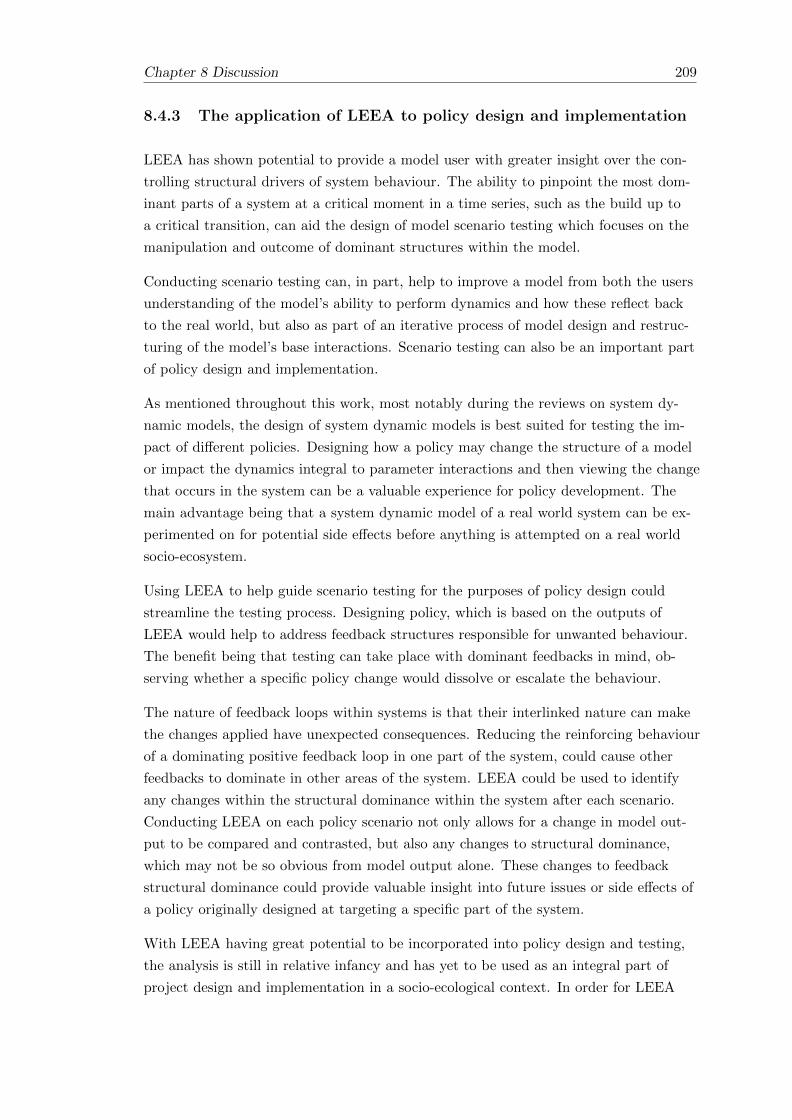
Chapter 8 Discussion 209
8.4.3 The application of LEEA to policy design and implementation
LEEA has shown potential to provide a model user with greater insight over the con-
trolling structural drivers of system behaviour. The ability to pinpoint the most dom-
inant parts of a system at a critical moment in a time series, such as the build up to
a critical transition, can aid the design of model scenario testing which focuses on the
manipulation and outcome of dominant structures within the model.
Conducting scenario testing can, in part, help to improve a model from both the users
understanding of the model’s ability to perform dynamics and how these reflect back
to the real world, but also as part of an iterative process of model design and restruc-
turing of the model’s base interactions. Scenario testing can also be an important part
of policy design and implementation.
As mentioned throughout this work, most notably during the reviews on system dy-
namic models, the design of system dynamic models is best suited for testing the im-
pact of different policies. Designing how a policy may change the structure of a model
or impact the dynamics integral to parameter interactions and then viewing the change
that occurs in the system can be a valuable experience for policy development. The
main advantage being that a system dynamic model of a real world system can be ex-
perimented on for potential side effects before anything is attempted on a real world
socio-ecosystem.
Using LEEA to help guide scenario testing for the purposes of policy design could
streamline the testing process. Designing policy, which is based on the outputs of
LEEA would help to address feedback structures responsible for unwanted behaviour.
The benefit being that testing can take place with dominant feedbacks in mind, ob-
serving whether a specific policy change would dissolve or escalate the behaviour.
The nature of feedback loops within systems is that their interlinked nature can make
the changes applied have unexpected consequences. Reducing the reinforcing behaviour
of a dominating positive feedback loop in one part of the system, could cause other
feedbacks to dominate in other areas of the system. LEEA could be used to identify
any changes within the structural dominance within the system after each scenario.
Conducting LEEA on each policy scenario not only allows for a change in model out-
put to be compared and contrasted, but also any changes to structural dominance,
which may not be so obvious from model output alone. These changes to feedback
structural dominance could provide valuable insight into future issues or side effects of
a policy originally designed at targeting a specific part of the system.
With LEEA having great potential to be incorporated into policy design and testing,
the analysis is still in relative infancy and has yet to be used as an integral part of
project design and implementation in a socio-ecological context. In order for LEEA

210 Chapter 8 Discussion
to reach a greater potential where it can benefit policy design in such a manner as de-
scribed above, it must become better known within the academic field, and its output
must be portrayed in terms of what is useful for a policy design team.
Being able to show what the driving influential structures within a system model are
may be interesting to a policy maker, but not useful without the context of how that
information can be used to change the system as required. In light of this, showing
what feedback loops are dominating a system may not prove useful without first con-
ducting further research in how to interact and change those feedbacks in the model’s
real world counterparts. Local knowledge of the system and capabilities of local in-
dustries becomes necessary to link model theory to practical change. This is where
DDWA, LEEA’s sibling analysis comes in, providing the ability to identify high influ-
encial parameters inside of feedback loops.
8.4.4 Acknowledging LEEA’s limitations in the context of ecological
modelling and policy making
From its most basic stand point, the purpose of a model is to help to bring assump-
tion and biases on the target system together (Holling and Chambers 1973). So, in
the first instance would LEEA help or hinder this process? Would a general under-
standing of how feedback loops interact and control a system aid or complicate the
dialogue that must occur across disciplines and especially between ecologists, policy
makers and local companies. As shown within this thesis, there is no doubt that un-
derstanding feedback loops within a system model through LEEA can greatly increase
the understanding of how a target system works. However, is the language used in
LEEA and the outputs it creates (eigenvalue plots, loop influence plots, loop influence
point plots) transferable in the context of policy design and implementation?
Policy makers and local businesses may not have the time to learn how to interpret
LEEA and what its outputs mean. With an overall understanding between parties
that models can be complex and analysis outputs take time to interpret, it would be
put upon the ecological modeller to convey the information from the analysis (in this
case the outputs of LEEA) quickly and clearly. With that in mind, pointing at a series
of lines from multiple line plots which LEEA produces may not be the best solution to
convey important information regarding the system’s feedback loops. Instead, convey-
ing the information from LEEA’s loop influence plots back into cyclic diagram form,
which all parties may have been involved in building at early stages of the modelling
process and where loop structures are easy to see, would greatly improve speed and
understanding for delivering key information from the analysis.
In real policy and decision making contexts data for every variable in the system is
often unobtainable, or limited at best, which presents a distinct limitation for using

Chapter 8 Discussion 211
LEEA. In situations where qualitative interactions are crucial or actors are strategic
and adaptive, LEEA would not be able to account for the actions of these players,
unless they were inherently described within the system’s dynamics. This presents a
common modelling problem of how to quantify concepts such as free choice or spon-
taneity within a model system.
LEEA fills an important niche as a model analysis tool which specialises in feedback
loops, but it is limited by its requirement of the whole system model having associated
dynamics and data. With all this in mind, LEEA’s practical application to policy and
decision making may best serve as an illustrative and critical thinking tool used best
in conjunction with other modelling forms. It might be in the best interest of deci-
sion makers to apply their strategies to an appropriate mix of models, not all of which
LEEA may be applicable to.
8.5 Exploring LEEA’s limitations
The limitations affecting LEEA include limited application to low feedback models,
practical limitations of the LEEA algorithms to system dynamic functions (i.e. STEP,
IF, etc.), but increasing complexity and number of results with larger models is the
most prevalent limitation restricting LEEA’s utility across multiple model scales (Oliva
2016; Kampmann and Oliva 2006). To explore this limitation further and gain first
hand understanding of interpreting results from increasingly complex models, PLUM-
Gov and PLUMPlus were generated as extensions to the PLUM model within chapter
5.
The PLUMGov and PLUMPlus models explored how incorporating multiple endoge-
nous dynamics into the PLUM model would affect the output gained from LEEA
and our ability to recognise a critical transition dynamic from the original PLUM
model. During analysis, it was observed how much of a difference if any, the addi-
tional features made to the output of PLUM. During LEEA analysis of PLUMGov
and PLUMPlus, three features were expressed in the analysis output which had been
identified as potential complications:
1) LEEA produces a lot of graphical data: Both Elasticity and Influence are generated
as part of LEEA output and can both be used to infer structural drivers of system
behaviour, but their output can differ greatly and must be interpreted separately as
they do not mean the same thing. Throughout this thesis the main focus has been on
interpreting loop influence values as these are generally considered to be the easiest to
understand. Loop influence plots are also considered the most accessible to an outside
reader and the outputs are not affected by eigenvalues which sit close to zero.

212 Chapter 8 Discussion
The PLUMPlus model showed how simple additions to model size and structure could
make profound changes to a model’s number of interactions, number of feedback loops
and therefore analysis results. One of the most important discussions contained within
the PLUMPlus study was interpretation of LEEA results became more challenging
when multiple eigenvalues had to be interpreted simultaneously.
One feature of LEEA is that it outputs a multitude of data regarding a system’s feed-
back loops corresponding to different eigenvalues. A large amount of analysis data to
interpret can be seen as having both a positive and negative side. While more data to
interpret and understand the system can be a good thing, the output of LEEA must
be filtered in order to identify the most prominent drivers. This is largely achieved by
identifying the eigenvalue expressing the greatest magnitude as this reflects the sys-
tem’s most dominant mode. However, when multiple eigenvalues express high values
at the same time, their elasticity and influence values must be interpreted simultane-
ously. If the outputs from these multiple sources contradict each other, i.e. showing
different loops dominating the system’s behaviour at the same time, then interpreta-
tion and reflection back on the real world system can be difficult.
2) Our ability to interpret LEEA’s outputs: Eigenvalues will contain complex numbers
when the system is expressing oscillatory behaviour. This in turn affects the elasticity
values and influence values output by LEEA, which also have complex values. Con-
taining complex values means that there is both a real and imaginary part which must
be interpreted in order to understand the feedback loop’s impact on the system.
Alongside having to deal with complex numbers, loop plots of both elasticity and in-
fluence can be difficult to interpret purely based on the number of feedback loops in
the system. Chapter 5 showed the PLUMPlus model which had a total of 17 feedback
loops, each of which had their own trajectory to be interpreted for a given behaviour
of the system and whose values could easily differ drastically between eigenvalues as
well as between elasticity and influence plots of the same eigenvalue.
Outputs of loop elasticity and influnece plots can sometimes appear counterintuative.
As an example, on loop influence plots, a negative feedback loop could display positive
real values inferring that it is generating instability within a system or vice versa with
a positive feedback loop displaying negative real values. While negative feedback loops
are usually associated with stabilizing behaviour and positive feedbacks with desta-
bilizing behaviour, the interaction and reinforcing behaviour held between feedbacks
on top of properties internal to feedback structures, like a delay in an interaction, can
cause feedbacks to express unexpected and sometimes opposite behaviours.
3) Artificial ‘Ghost’ loops: Ghost loops occur when the elasticity or influence value of
a loop is reflected by another loop in the opposite polarity, effectively counteracting
each other’s influence. The presence of ghost loops can mean that a loop appearing

Chapter 8 Discussion 213
to express a high level of influence over the system is being countered by the dynam-
ics within another loop. Sometimes this counter-action occurs across only a section of
a time series and the two loops no longer mirror each other when the system changes
behaviour. When a model contains artificial loops it can infer a problem with the dy-
namics and structure of the model, not reflecting the real world system correctly.
Limitations in validating LEEA and its outputs
As pointed out from the literature review alongside a discussion within chapter 5 of
the PLUMPlus model, validation of LEEA and its outputs take the form of an inter-
nal and an external validation. The internal validation links to validation of the model
LEEA is analysing, whilst external validation requires data collection and compari-
son to the real world. Data collection alongside model and output validation can, at
the best of times, be difficult to achieve due to impracticalities or economic feasibility.
Data validation is a universal issue across all models and a user would benefit to bear
this in mind when thinking of using LEEA for a project.
8.6 LEEA in Qualitative Modelling
8.6.1 Early Model Design and consequences to LEEA: A Case Study
Qualitative research can play an important role in the early stages of model design
and development, which ultimately determine the structural representation and dy-
namic properties of a system model. In turn these perceptions of the target system
have great impacts on the outputs gained from loop analysis. The following section
discusses a project conducted by the author in January of 2016 alongside a research
group at the Harbour Branch Oceanographic Institute, at the University of Florida.
The project investigated a prominent microbial species of freshwater lakes, Loxodes
Rex (Hines et al. 2016), and its effects on surrounding freshwater lake systems using
specialist knowledge of micro-biological systems, socio-ecology and local food webs.
Initial intentions of the project were to construct a system dynamic model of the local
ecosystem and use LEEA to investigate the feedback loops which the newly discovered
species Loxodes Rex could be influencing. Unfortunately due to limitations of avail-
able data and time constraints set for the project, a model accurate enough to reflect
the target lake system could not be developed. Despite this, through the practices
adopted by participatory complexity science, qualitative data and local knowledge of
the system were enough to construct a structural representation of the target system.
The cyclic diagrams produced proved to be an invaluable talking point with which to
focus the remainder of the study, investigating methods of dispersal of Loxodes rex

214 Chapter 8 Discussion
from local to regional scales, and could be used as a platform on which to build an ef-
fective system dynamic representation of the system in the future. Some outputs of
this project can be seen below.
Loxodes Rex. Local vs Regional interactions
An organism’s ability to populate a large region is controlled by properties of the lo-
cal habitat alongside regional processes which facilitate dispersal (Havel and Shurin
2004). While studies of local habitat properties investigate controlling factors of popu-
lation growth rates i.e. temperature, salinity, predator population and food availability
(Finlay et al. 1986, Finlay and Berninger 1984), regional studies of dispersal tend to
concentrate on the physical mechanisms by which the organisms spread (Wilkinson
et al. 2012, Green and Figuerola 2005, Havel and Shurin 2004).
The bulk of the case study focused on network properties at regional scales which af-
fect the species dispersal capabilities. To aid discussion, a cyclic diagram was con-
structed at the beginning of the project and subjected to an iterative process of de-
sign, discussion and redesign to visualise the complex nature of interactions and feed-
back processes which affect the local capability of Loxodes rex to populate its environ-
ment as shown in figure 8.2. This figure was used as a reference point throughout the
project, particularly concerning the ecological contribution Loxodes rex makes towards
its local ecosystem.
The project began by using system dynamics to investigate the freshwater bodies of
Florida and building a structural representation of the drivers which affect the sur-
vival of Loxodes rex. The project then moved onto studying the ability for the Lox-
odes rex to successfully colonise a single water body and finally, investigating proper-
ties of a system which would allow the species to successfully spread across the entire
State of Florida.
Building a Cyclic Diagram and System Dynamic Model
Constructing a cyclic diagram at the early stages of the project proved a valuable as-
set to the research group as it allowed discussion points to be made from a common
level of understanding about the target system. This also kept the discussion cen-
tralised around the concepts of parameter interactions and vital vs. unnecessary com-
ponents, which in turn made the transition from initial discussions to system dynamic
model much smoother as the entire team working on the project could see how the
model had been developed and justify its structure and components. Overall the cyclic
diagram provided the group with a visual output of system interactions, consolidating
all of their knowledge of the system into one simple diagram. It provided an excellent
base and reference point to return to during any discussion within the project that
could be easily adapted and adjusted as the project developed.

Chapter 8 Discussion 215
Figure 8.2: Cyclic diagram of factors affecting the success of a population of Lox-odes rex
While limited data was available to begin running model scenarios specific enough to
reflect the target system, the cyclic diagrams were converted into a system dynamics
format (figure 8.3) in order to gain information regarding the structural properties of
the system. This model had significance not only in investigating the system’s feed-
back mechanisms present, but was designed to be able to conduct LEEA and sensi-
tivity analysis on the system drivers pending more data at a later stage. LEEA was
discussed as a tool with the potential to identify dominant structures of the ecosystem
at critical times during the growth and colonization by Loxodes rex.

216 Chapter 8 Discussion
Figure8.3:
Syst
emd
yn
amic
sd
iagr
amof
the
syst
emd
rive
rsan
din
tera
ctio
ns
aff
ecti
ng
Lox
od
esre
xw
ith
init
slo
cal
fres
hw
ate
ren
vir
on
men
t.
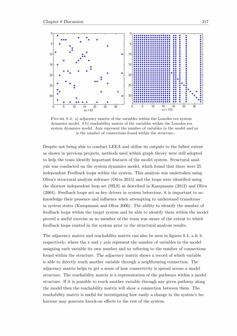
Chapter 8 Discussion 217
Figure 8.4: a) adjacency matrix of the variables within the Loxodes rex systemdynamics model. 4 b) reachability matrix of the variables within the Loxodes rexsystem dynamics model. Axis represent the number of variables in the model and nz
is the number of connections found within the structure..
Despite not being able to conduct LEEA and utilise its outputs to the fullest extent
as shown in previous projects, methods used within graph theory were still adopted
to help the team identify important features of the model system. Structural anal-
ysis was conducted on the system dynamics model, which found that there were 25
independent Feedback loops within the system. This analysis was undertaken using
Oliva’s structural analysis software (Oliva 2015) and the loops were identified using
the shortest independent loop set (SILS) as described in Kampmann (2012) and Oliva
(2004). Feedback loops act as key drivers in system behaviour, it is important to ac-
knowledge their presence and influence when attempting to understand transitions
in system states (Kampmann and Oliva 2006). The ability to identify the number of
feedback loops within the target system and be able to identify them within the model
proved a useful exercise as no member of the team was aware of the extent to which
feedback loops existed in the system prior to the structural analysis results.
The adjacency matrix and reachability matrix can also be seen in figures 8.4, a & b
respectively, where the x and y axis represent the number of variables in the model
assigning each variable its own number and nz referring to the number of connections
found within the structure. The adjacency matrix shows a record of which variable
is able to directly reach another variable through a neighbouring connection. The
adjacency matrix helps to get a sense of how connectivity is spread across a model
structure. The reachability matrix is a representation of the pathways within a model
structure. If it is possible to reach another variable through any given pathway along
the model then the reachability matrix will show a connection between them. The
reachability matrix is useful for investigating how easily a change in the system’s be-
haviour may generate knock-on effects to the rest of the system.

218 Chapter 8 Discussion
Despite this section of the project stretching little beyond the capabilities of quali-
tative research, the team found that the system dynamics approach provided a new
perspective for thinking about the systems main properties and interactions. Overall
it was found that the initial methodology of systems thinking, visualising systems in
terms of their interactions of components and being able to go through an iterative
process of model design as a team benefitted the project greatly. Iterations of causal
loop diagrams aided group discussion and gave the project a platform with which to
find common ground as well as a focus with which to forward the project. The initial
stages of this project lead to more confidence in the model structure and dynamics im-
posed on the interactions which would have the knock on effect of interpreting LEEA’s
results from a platform of confidence about the system model and understanding of
the natural system when interpreting the output of influential loop structures.
8.6.2 Is There A Place For Qualitative Modelling Within System
Dynamics?
As in the model construction of the Loxodes Rex. project, it can become apparent
that there is not enough data or information in order to input quantitative data into
every part of the system in order to run an accurate system dynamic model. Qualita-
tive modelling in the field of system dynamics is a process of formulizing and analysing
feedback loops without the process of simulating numerical output. Qualitative mod-
elling of a system is otherwise known as soft Operational Research (OR) and occurs
when quantitative modelling is either not possible or is undesirable (Coyle 1998). In
OR, the structure of the model itself becomes a platform for discussion and learning.
A recurring question within the literature of system dynamics seems to be whether
qualitative modelling has a place in the technique, or whether only quantitative meth-
ods leading to simulation hold a place in system dynamics. The phrase “When to map
and when to model?” was coined by Richardson (1996) concerning the uses of qualita-
tive vs quantitative system dynamic modelling.
It is generally accepted across the field of system dynamics, as discussed in Luna-
Reyes and Andersen (2003) and first illustrated in Forrester (1994), that the amount
of information available about a system decreases sharply as you go from a mental
model (observations and experience) to a written data base, to a numerical data base.
Starting from qualitative information and trying to provide quantitative data for every
variable can be challenging.
System dynamic models are mathematical representations of problems and policy al-
ternatives where often most of the information available to the modeller is not numeri-
cal in nature (Luna-Reyes and Andersen 2003).

Chapter 8 Discussion 219
While using quantitative data, there is the question of how much weight can be at-
tributed to it: Who sourced the data? Was it from the client of the modelling process
or the consultant? Might the collector of the data have had any bias towards the out-
put? The validity of the simulation has to be questioned when there is so much uncer-
tainty in the parameters of the model.
Data collected on a variable can differ depending on the individual doing the record-
ing. For example, if a person were to record the temperature in a room, you could put
24C or ‘hot vs cold’. Modellers do not always have the privilege of asking how they
require data to be collected or have the ability to go back to record data themselves.
In the context of LEEA, the analysis cannot be run unless there is data with which
to simulate the model. This would suggest that only a quantitative approach where
differential equations and empirical data is available is important for LEEA. However,
the outputs and interpretations of LEEA are so heavily reliant on a model’s structure,
that the qualitative stage of model design, interatively building a system’s internal
structure with a system’s thinking approach (i.e. first representing the system with a
causal loop diagram), should not be overlooked.
The following sections discuss qualitative modelling in the context of system dynamic
modelling:
For:
In system dynamics, the importance of studying behavioural patterns has always been
stressed, especially when the data is limited. But this is not wise when a client (for
whom you are creating the model) believes that they are retrieving precise data from
the model’s output. “Omitting structures or variables known to be important because
numerical data are unavailable is actually less scientific and less accurate than using
your best judgement to estimate their values” (Sterman 2000).
Nuthmann (1994) coins the phrase ‘plausible nonsense in our models’ referring to the
practice of quantifying a model without fully being able to validate the data going in
and therefore producing output which seems correct, but in fact does not reflect the
real world.
System dynamic models and causal loop diagrams are often capable of producing pol-
icy insights before any form of simulation is conducted because of how they map out
system structure in a highly visual manner and are capable of showing large amounts
of information in a single diagram. Coyle (1998) recounts of how a system about in-
stability in Africa which was described over a series of 50 written pages was able to be
represented by a causal loop diagram containing 57 variables and 200 links. While this
diagram was far from simple, it did allow for all of the information about the system’s
structure to be visualised on a single page.

220 Chapter 8 Discussion
An example of qualitative data having practical uses is demonstrated in Coyle et al.
(1999) who shows how new insights can be gained from a qualitative diagram of the
treatment of psychogeriatric patients. Coyle shows how policy insights may be mapped
onto an existing qualitative diagram. The diagram is capable of showing where infor-
mation flows may be lacking or blocked from getting to the right people (in this case
the medical staff of the facility) and this is purely determined by examining the sys-
tem’s structure, prior to or foregoing any simulation.
An example of the difficulties which arise when attempting to quantify data can often
be seen when trying to model human choice or perception, a topic which is relevant
to the field of soico-ecology. System dynamic models can be difficult to quantify more
often than not when social components are required to be incorporated into the struc-
ture. For example tourist satisfaction at a resort may be represented on a scale of 1 to
5, but scales such as this can differ between each individual so it is difficult to quantify
what 100% satisfaction is if compared to 50%. Likewise, when it comes to quantifica-
tion of a variable with two potential outcomes (i.e. more likely to vote for party X or
party Y) it is often tempting to enforce a multiplier from 0 to 1 which represents two
extreme views of the choice, but this type of quantification runs into trouble when the
value reaches 0.5 as it is uncertain what this would represent.
Coyle et al. (1999) points out that while you cannot infer dynamic behaviour simply
from a complex diagram, being able to describe a system and visualise its structure
has a use in itself. Coyle summarises the uses of influence diagrams (those which do
not undergo simulation):
• They can condense multiple pages of description onto a single diagram.
• They are able to form a type of agenda and be useful at discussion meetings
about the system.
• Identifying key structures in the system i.e. feedback loops can give insight into
possible system behaviour.
• Studying the diagram may reveal the wider contexts of the modelling task.
• Finally they are the basis with which to start an informed quantified model.
Luna-Reyes and Andersen (2003) recount benefits of qualitative modelling which in-
clude: understanding of the modelling process, facilitate communication among mod-
ellers and clients and set up methodological framework to promote constructive dis-
cussion around the merits of qualitative versus quantitative modelling.
Against:
Chapter 8 Discussion 221
It is often accepted that in order for a system dynamic model to be applicable to guid-
ance and policy, it must be possible to fully quantify (attribute equations and data to)
its components.
Common forms in which qualitative data is collected include: interviews, oral history,
focus groups, delphi groups (an extension of focus groups making use of survey and
interview analysis), observation, participant observation and experimental approaches.
An explanation of all of these may be found in Luna-Reyes and Andersen (2003). The
main cost of collecting qualitative data in this manner is that it is time consuming
and labour intensive, often having to go through an ethics check system as much of
the data gathered can involve the public.
Despite the growing popularity of system dynamics and its growing use across multi-
ple disciplines, (Lane 1999, Guo et al. 2001, Saleh et al. 2010) Forrester expresses how
a lack of system dynamics in the education system and a lack of training at the indi-
vidual level has created a rift between the practice of system dynamics (a quantitative
approach) and the practice of System Thinking (a qualitative approach). Forrester
(2007a) explains how System Thinking often tries to dumb down the concepts intro-
duced in system dynamics, often through causal loop diagrams or management games
which focus on decision making. However, the true power in system dynamics lies be-
hind how policy design influences those decisions.
“ Making system dynamics simple is a losing game. System dynamics is not simple.
The problems of complex feedback systems are not simple.” (Forrester 2007a)
While Forrester expresses how the origin of system dynamics focused on tackling ma-
jor issues in the outside world, he criticises how much of the real world relevance has
been lost to its use in academic papers (Forrester 2007b). Forrester (2007b) explains
that system dynamics as a field has not taken the necessary steps that would give it a
place in important issues including: trade deficits, the future of social security, immi-
gration and political promises in the healthcare sector. Instead system dynamics has
been misrepresented through a lack of proper training at both an individual and insti-
tutional level as well as a drive for academic paper publication rather than real world
issues.
8.7 The future for LEEA - Steering Complex Systems
Given LEEA’s strengths for identifying driving structures within a system and its
ability to identify system leverage points, while also accounting for the limitations
which a user of LEEA would face in terms of data collection and utility to a policy
maker, it is important to consider its utility for the future. As it stands, LEEA’s method-
ology is best suited as a key component of a ‘steering complex systems’ approach. As

222 Chapter 8 Discussion
shown from the case study within chapter 6 of this thesis, LEEA is an extremely use-
ful and informative method when used on its own, but the knowledge gained from its
output becomes even more valuable when used alongside other techniques which to-
gether uncover and/or detect key and dominant parts of a system.
LEEA’s role in future projects lies in the exploitation or mitigation of system feed-
backs as effective levers. LEEA would provide a significant benefit alongside projects
which prioritised system structure and component interaction as key focus points dur-
ing model construction. LEEA’s outputs would provide more utility to projects in
which local authorities and local companies were involved to help differentiate between
dominant system levers identified within LEEA and effective system levers which were
physically, ethically and economically viable to manipulate. Finally, LEEA would ben-
efit projects which used an array of analysis tools in order to gain the model knowl-
edge out of their model. LEEA is built to provide a wealth of information regard-
ing the feedback loops within a complex, dynamic system and in comparison to all
other methodologies identified within this thesis, is almost unparalleled in its ability to
do so, but its methodology has limited utility outside the scope of system feedbacks.
Used in conjunction with other analysis techniques, LEEA has considerable potential
for a future in ‘steering complex systems’, having great utility in its niche for identify-
ing and analysing system feedback loops.
8.8 Future Work - What Next?
LEEA needs to be utilised on a wider range of model subjects in order to continually
test its utility to a range of SES dynamics. The more dynamic behaviours and sys-
tems which LEEA is used to analyse, the greater idea we get of its applicability to all
system dynamic models. In this thesis, LEEA has been shown to provide novel insight
into key questions and concerns surrounding lake systems and coral reef ecosystems,
but this does not mean that LEEA has a place in all studies of lake or coral reef mod-
els. LEEA will not be appropriate for all system dynamic models as demonstrated
within Chapter 5 of this thesis, which explored the limitations of LEEA, but it will
certainly have a greater application to critical transitions, or determination of bistabil-
ity than that which is explored within this thesis.
The next logical step would be to use LEEA within a research site (such as a coral
reef environmental centre or fishery research centre) where the model can be designed
based on variables and interactions specific to that location where the data for the
model is readily available. The analysis would be used to gain information of the sys-
tem drivers which can then be compared and used alongside existing knowledge of
the researchers and, testing its applicability to real world system in real time (i.e.

Chapter 8 Discussion 223
a week by week basis of data collection to model analysis output). The system dy-
namic model of the project can be designed with conducting structural loop analysis
in mind, even utilising LEEA’s ability to identify the extent of dominance within the
system as part of the model testing and validation.
Improvements can be made to LEEA’s automation. The most recent update to its
online capabilities occurred in Sept 2017. It is important that the analysis and its de-
velopment is live and is active, i.e. is still ongoing as this means that the utility of the
technique is still improving. As mentioned previously within this discusson, the ability
to gain analysis output simultaniously with model runs would greatly streamline the
process of conducting LEEA and have many benefits with regards to instant feedback
on changes to model structure made during scenario testing. This process would not
come without its limitations, as the multitude of data LEEA outputs and the user’s
ability to select relevant data would still be an issue.
Design and creation of a common ground with which to explore and share the mod-
els and dynamic behaviours that LEEA has been used to analyse, could provide a
database for the successes and failures of the technique across a range of disciplines.
An online platform with which to search for specific dynamic behaviours or find other
models of similar target systems where LEEA has already been used to great effect
could greatly benefit the wider modelling community, as well as improve the accessibil-
ity and effectiveness of LEEA.
From personal observations and searches conducted by the author, there are many
system dynamic models used within the SES community, but they are not always
made readily available for further analysis. Sometimes, papers will display their sys-
tem dynamic model, but not fully disclose the dynamic equations associated with that
model. Often reproducing a model and its results is not possible as values used within
the model are not stated or included within additional information sections. Often
system dynamic models in SES appear to be used to generate an output and then
not used any further which reduces the potential information gained from the model
and prevents analysis like LEEA being easily run on the system. These types of infor-
mation blocks need to be challenged alongside looking for new and alterative analysis
techniques as one cannot be used to its full potential without the other.
8.9 Importance of Accessibility: A Review of LEEA Im-
plementation and Subject Terminology
8.9.1 Improving LEEA Accessibility
With greater testing and implementation over a wider variety of systems, LEEA has
potential to be a useful analysis tool across a wide range of socio-ecological projects

224 Chapter 8 Discussion
and find itself as a mainstream analysis. However, for it to first be considered by the
wider academic community and be justifiable as a tool for policy manipulation, its
accessibility to academic, public and political audiences must be addressed.
Socio-ecology is by definition, a multidisciplinary field joining together social sciences,
with environmental science, ideally capable of integrating all of the techniques used
therein, capable of producing more accurate and realistic models. Model users within
the SES field will approach LEEA with varying levels of knowledge, particularly sur-
rounding their numerical and modelling background. For LEEA to be available to
academics of multiple disciplines, it must have a standardised format from which to
learn about and implement the technique. Implementing LEEA requires understand-
ing of several concepts which are not all found within the same line of research e.g.
knowledge surrounding feedback loops, eigenvalues, graphy theory and linear stability
theory are all required in understanding LEEA, but their theory does not go hand in
hand. A user must search multiple different areas/disciplines of research in order to
gain full understanding of each step that LEEA undertakes. This is currently a great
deal of extra work and effort required on the user’s part and with little prior knowl-
edge, the learning curve to understand Jacobian matrices, eigenvalues, system dynam-
ics, Mathematica coding etc. can be steep. The current requirement to learn LEEA
may be unwelcomed as much of the theory which the user comes across may be irrel-
evant in order to understand LEEA. A single place where the information required to
learn and implement LEEA is consolidated and standardised would greatly improve
LEEA’s accessibility for a wide academic audience.
Naumov and Olivas online materials (Naumov & Oliva 2017) provide a great platform
to implement LEEA, automating many of the required calculations: the Jacobian ma-
trix, eigenvlaues, loop gains, loop elasticities and loop influence values. R. Oliva even
provides a package to convert Vensim diagrams (a software for constructing system
dynamic models) into a format mathematica can use.
The code can be prone to minor errors, which can be difficult to find the source of if
the user is unfamiliar with the code. An error which occurred frequently was due to
model variable names being the same as variables used to run the code, i.e. shortening
a variable of rainfall to ‘r’ would overlap with a coding variable and cause the LEEA
package to stop working.
The code currently contains each step of LEEA in a separate section which helps to
translate the required steps of LEEA into the order in which the package carries out
calculations. To improve accessibility, the introduction of each section and the nota-
tion within could be extended to better explain how the code processes each calcula-
tion. This would increase user understanding of code function and aid the identifica-
tion of errors.

Chapter 8 Discussion 225
Finally a common, open access place in the form of website or forum could be ini-
tialised for users of the analysis to share findings, uses and errors of the analysis and
associated software. Having a common place with which to share experience would
benefit individual users seeking advice and feedback, as well as improving the overall
analysis by identifying errors in the base code and providing extensions which individ-
ual users have built for specific projects.
8.9.2 Accessibility of system dynamic modelling to the public and
policy makers
Making system dynamic models accessible is important, not just for outreach pur-
poses, but also for the ability to communicate with businesses and industries which
could be major players in a restoration or conservation project.
As it currently stands, system dynamics is accessible to a public audience as a vi-
sual method of modelling, which can be understood with some basic understanding
of stocks and flows. Causal flow diagrams can also be used as a more simplified ver-
sion of a system dynamic model so that dynamics do not need to be considered and a
focus can be drawn to the components and interactions of the system.
However, system dynamic models are not trivial. Before any analysis is conducted,
models naturally begin to get complicated as they grow in size; the ability to follow an
individual chain becomes harder; the links between stocks become more complex and
the ability to pick out feedback structures becomes more difficult.
8.9.3 Discussion on the terms positive and negative feedback:
Positive and negative feedback have long been terms used to describe the two states
which feedback loops can form. Understanding how they form, what they look like
and what behaviours they are capable of generating is fundamental within the study
of system dynamics and structural loop analysis. This section reflects on the terms
positive and negative in terms of system dynamic feedback and explains how both
are inappropriate and misleading and calls for an appropriate alternative to be intro-
duced/ maintained within the field of system dynamics.
The very first time that we are introduced to the terms of positive and negative feed-
back is within the education system of primary and secondary school. From this envi-
ronment we learn that positive feedback is something useful and encouraging, overall
being a good thing, while negative feedback is seen as unhelpful and at times harsh,
often viewed as something that would not be of any benefit. Unfortunately, in terms
of system dynamics, these preconceptions can create a skewed and often false view
of what positive and negative feedback loops mean for a system. Positive feedback in
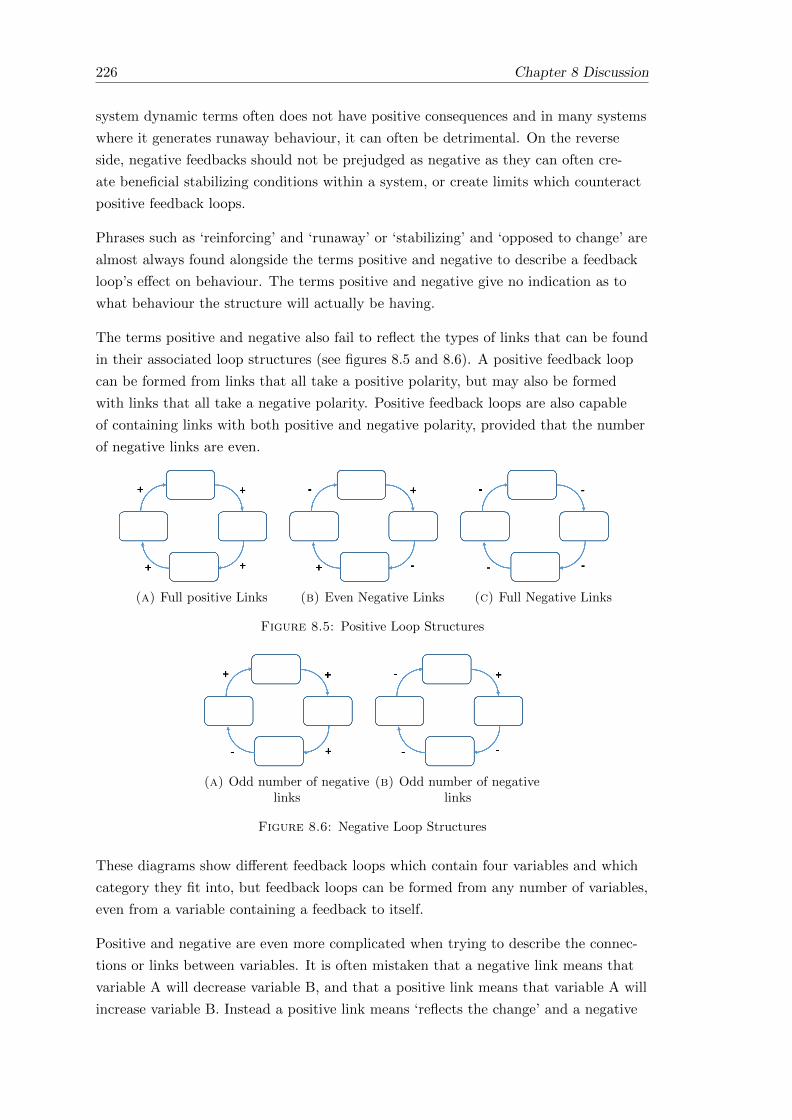
226 Chapter 8 Discussion
system dynamic terms often does not have positive consequences and in many systems
where it generates runaway behaviour, it can often be detrimental. On the reverse
side, negative feedbacks should not be prejudged as negative as they can often cre-
ate beneficial stabilizing conditions within a system, or create limits which counteract
positive feedback loops.
Phrases such as ‘reinforcing’ and ‘runaway’ or ‘stabilizing’ and ‘opposed to change’ are
almost always found alongside the terms positive and negative to describe a feedback
loop’s effect on behaviour. The terms positive and negative give no indication as to
what behaviour the structure will actually be having.
The terms positive and negative also fail to reflect the types of links that can be found
in their associated loop structures (see figures 8.5 and 8.6). A positive feedback loop
can be formed from links that all take a positive polarity, but may also be formed
with links that all take a negative polarity. Positive feedback loops are also capable
of containing links with both positive and negative polarity, provided that the number
of negative links are even.
(a) Full positive Links (b) Even Negative Links (c) Full Negative Links
Figure 8.5: Positive Loop Structures
(a) Odd number of negativelinks
(b) Odd number of negativelinks
Figure 8.6: Negative Loop Structures
These diagrams show different feedback loops which contain four variables and which
category they fit into, but feedback loops can be formed from any number of variables,
even from a variable containing a feedback to itself.
Positive and negative are even more complicated when trying to describe the connec-
tions or links between variables. It is often mistaken that a negative link means that
variable A will decrease variable B, and that a positive link means that variable A will
increase variable B. Instead a positive link means ‘reflects the change’ and a negative

Chapter 8 Discussion 227
link means ‘opposes the change’. To this end, even the symbols that are commonly
used to visualise these structures ‘+’ and ‘-’ are misleading.
Overall the terms negative and positive when discussing system dynamic structures
are counterintuitive to making the field accessible to a wider audience. The terms nei-
ther describe the system structures in terms of their internal links, the output they
produce, nor their potential benefit/detriment to the system. New names for these
terms could increase clarity and accessibility to public audiences and educational plat-
forms. The terms ‘reinforcing’ and ‘stabilizing’ for feedback loops and ‘reflects change’
and ‘opposes change’ for causal links may not be appropriate for all scenarios, but are
an example of four terms which give a better indication of the structure’s capabilities.


Chapter 9
Conclusions
Loop Eigenvalue Elasticity Analysis (LEEA), a structural loop analysis tool for sys-
tem dynamic models has been shown to have great potential for use in ecological and
soico-ecological study. The principles on which it is based; identifying system struc-
tures as drivers of dynamic behaviour and attributing behavioural shifts to changes in
feedback loop dominance are complimentary to evidence and theory surrounding many
processes within socio-ecological systems. LEEA has been found to be an important
tool to consider in a socio-ecological project, not for its ability to determine system
stability, nor for its ability to attribute system behaviour to feedback loops as these
are important features, but are already well known. The power gained from LEEA’s
utility lies in the ability to disentangle and prioritise feedback loops within a system
from the ‘black box’ models on which our simulations rely. LEEA provides greater un-
derstanding and therefore control over our model systems.
LEEA’s utility naturally matches and is able to compliment key dynamics which are
hot topics within the conservation, sustainability and resilience communities. It excels
at analysing and shedding light on non-linear processes including oscillations, system
collapse, exponential growth and decay and has been shown within this thesis to have
a practical use in studies of critical transitions, hysteresis and mono vs. bistability.
Despite its great potential, LEEA like many techniques of its kind does not come
without practical limitations. A user’s ability to interpret LEEA becomes increasingly
difficult with model size and complexity. While this may not be such a problem for
experienced users of the technique, one of the aims of this thesis is to introduce LEEA
analysis and its way of thinking about complex system drivers to a new audience of
socio-ecologists and therefore it is important to highlight this limitation to new users.
The utility of LEEA hits a plateau when its output becomes just as complicated to
interpret, if not more so than the complex model that is being analysed.
229

230 Chapter 9 Conclusions
One main interest of the meta analysis of LEEA was to see if it could have a use in
the design and implementation of environmental and conservation policy. To investi-
gate this, LEEA was examined within the context of system leverage points, accessing
whether the identification and quantification of dominant feedback loops could be jus-
tified as system leverage points and if so could they aid in the design of well informed,
efficient and effective environmental policy.
For the purposes of gaining a greater understanding over a model system and its drivers,
LEEA works well as a stand alone analysis and can provide the user with a wealth of
information which is not attainable from simple data output or from other analysis
techniques. However, when it comes to the identification of leverage points and its po-
tential use in policy, it would be ill advised to use LEEA as the sole justification for
policy design. LEEA’s output is purely numerical based on the dynamics internal to
the target system. LEEA does not therefore take into account concepts of a safe or
just operating space and its output does not take into account the practicality, eco-
nomic cost or ethics of manipulating dominant system structures unless these concepts
are integrated into a model’s structure and design.
LEEA has been shown within a lake system and coral reef system model. The empha-
sis within this thesis was exploring the breadth of LEEA’s utility, but many more sys-
tems where LEEA is effective could be explored. This cannot be achieved within one
thesis and needs to happen on a much wider scale across multiple different systems
world wide. Implementing an online platform where LEEA results could be shared
and discussed between model users would result in a common space with which to ex-
plore and understand dynamic behaviours and the interplay of feedback loops across a
multitude of complex systems.
The next step would be to use LEEA within a socio-ecological project where the sys-
tem’s dynamics were not already well known. There would be nothing to compare
the results of LEEA to and this would therefore give a new perspective on how use-
ful LEEA was and the extent that its results could be relied upon and utilised as the
main analysis tool of a project.
Supplementary Information
Supplementary Information 1: LEEA Methodology
The following calculations are required for LEEA analysis. A full breakdown of the
formula required for LEEA analysis can be found in Kampmann (2012) with the orig-
inal theory found within Forrester (1983) and Forrester (1982). A more detailed 10
step guide with model examples can be found in Guneralp (2006). Online material to
help streamline the analysis and avoid manual calculations (i.e. of the Jacobian matrix
and eigenvalues) can be found from Oliva (2015).
Calculation of loop eigenvalues and loop influence values is conducted via the follow-
ing process:
1. The Jacobian Matrix of the dynamical system model.
2. Eigenvalues of the Jacobian matrix.
3. Loop Gains.
4. Loop Eigenvalue Elasticity & Loop Influence.
1) The Jacobian Matrix The original model to be analysed must first be converted
into a series of partial differential equations (PDEs) and thus be cast as a dynam-
ical system in order to calculate its Jacobian matrix. The model may already exist
as a dynamical system (a set of differential equations) or as a system dynamic model
(SDM), which has to be interpreted as a dynamical system. The Jacobian Matrix is
an nxn square matrix and represents the links held between system stocks in their
most compact form (Goncalves 2009). Where each element of the matrix is equiva-
lent to taking the partial derivative of one stock with respect to another system stock
is a partial differential equation that represents how one stock affects another stock’s
derivative, when all other stocks are kept constant. The matrix therefore represents
the links between two stocks (Goncalves 2009). To calculate it, the differential equa-
tions for each stock of the system must be known. A Jacobian Matrix takes the gener-
alised form:
231

232 Chapter 9 Conclusions
J =
∣∣∣∣∣∣∣∣∂x1∂x1
. . . ∂x1∂xn
.... . .
...∂xn∂x1
. . . ∂xn∂xn
∣∣∣∣∣∣∣∣ . (9.1)
Where J is the Jacobian Matrix of the system and ∂x1∂xn
represents the change in net
rate of stock variable x1 in response to an infinitesimal change in the value of stock
variable xn. (Saleh 2005). The calculation of a Jacobian matrix requires the system
to be linearised. By calculating the entries of the matrix at any single point in time,
all non-linear inputs can be taken as constants and the model can be linearised at
that individual point in time (Kampmann 2012; Guneralp 2006; Forrester 1983). If
the model is to be linearised at each time step, then the time steps or changes in the
system between time steps, must be very small to assume linearity.
2) Eigenvalues of the Jacobian - Eigenvalues are calculated from a system’s Jacobian
matrix and therefore the number of eigenvalues of a system is equal to the number of
stocks in that system. Eigenvalues (λ) are calculated for an nxn matrix (A) by satis-
fying the equation: det(A − λI) = 0, where I is an nxn identity matrix. From linear
stability theory, eigenvalues can be used to determine if a system at a fixed point is
stable or unstable (Glendinning 1994). Eigenvalues are capable of being real, or com-
plex numbers with a real and imaginary part. If the real parts of all eigenvalues are
negative, then the fixed point is stable. If the real parts of any of the eigenvalues posi-
tive, then the fixed point is unstable.
In linear systems and particularly in matters of system stability and exponential growth/de-
cay, the dominant eigenvalue (i.e. the one with the greatest absolute value) should not
always be taken as the one most important to understanding the system’s behaviour.
If the real part of any eigenvalue within a linear system holds a positive value, no
matter how small its magnitude, it will eventually dominate the system’s behaviour
(Guneralp 2004; Emami-Naeini et al. 2002).
Changes in values to eigenvalues which sit at or close to zero are more likely to cause
shifts in polarity than highly negative eigenvalues. When concerned with system sta-
bility, eigenvalues changing polarity is an extremely important phenomenon to be
aware of, particularly when working with systems capable of experiencing critical tran-
sitions, regime shifts or system collapse. In the context of influential feedback struc-
tures, a shift in eigenvalue polarity often infers a change has occurred to which feed-
back loop is dominating within that eigenvalue. Changing from a dominant negative
feedback to a dominant positive feedback can lead to a reinforcing or runaway be-
haviour, which eventually destabilizes the system. With regards to system stability,
eigenvalues which sit at or close to zero and eigenvalues which hold large real positive
magnitudes can be seen as more important than eigenvalues with larger negative mag-
nitudes.
Chapter 9 Conclusions 233
In determining which eigenvalues are important to focus on, it is also important that
the user takes into account the changes that occur within an eigenvalue through time.
The build-up to an eigenvalue gaining dominance or changing polarity within a system
can be just as important for identifying feedback loops which are driving change than
taking eigenvalues at isolated points in time.
3) Loop Gains - Loop gain is required to compare perturbations within the system’s
feedback loops against the system’s eigenvalues. In order to calculate loop gain, the
gain of each causal link within that loop must first be determined. A causal link refers
to the link (edge) between two variables where a connection stems from a predecessor
variable and leads to a successor variable. The strength of a link, or ‘link gain’ refers
to the amount of influence a predecessor variable produces on a successor variable.
The gain of a causal link (a) is the partial derivative of a successor variable v1 with
respect to a predecessor variable v2:
av1v2 =∂successor
∂predecessor=∂v1∂v2
(9.2)
The gain of a loop (g) is then calculated through the product of all causal link gains
which join together to form that loop (Kampmann 2012):
g = av1v2 .av2v3 .av3v4 . . . . avnv1 =∂v1∂v2
.∂v2∂v3
.∂v3∂v4
. . . .∂vn∂v1
(9.3)
where v1,2,3,4n represent individual variables which link together to form a feedback
loop.
4) Loop Eigenvalue Elasticity is a measure of the importance of a loop on the system’s
current behaviour and is defined as the partial derivative of the eigenvalue with re-
spect to the gain of the loop, normalised to isolate the effect of changes in size (values)
of the eigenvalues and link gains (Goncalves 2009). It represents a relative change in a
system eigenvalue (λ) with respect to a relative change in the gain of a feedback loop
(Kampmann and Oliva 2008; Kampmann and Oliva 2006). One can attribute the im-
portance of a feedback loop to the absolute value of its loop eigenvalue elasticity. Loop
eigenvalue elasticity , is defined with respect to the loop’s gain parameter, in the form:
ε =∂λ
∂g.g
λ(9.4)
where λ is an eigenvalue of the Jacobian matrixsystem chosen by the user and g the
gain of a feedback loop as defined above. If the eigenvalue is a complex number:
λ = reiθ (9.5)

234 Chapter 9 Conclusions
where r = |λ| is the absolute value of the eigenvalue and is known as the “natural
frequency”, i is the imaginary value and cosθ is known as the “dampening ratio”, then
the loop eigenvalue elasticity will also be complex, holding real and imaginary parts:
R{ε} =dr
dg.g
r(9.6)
Im{ε} =dθ
dg.g (9.7)
It is possible to measure the real and imaginary parts of elasticity separately as shown
in Kampmann (2012):
ε1 =dRe{λ}dg
.g
|λ|(9.8)
ε2 =dIm{λ}dg
.g
|λ|(9.9)
These calculations are possible because the eigenvalues and loop gains of a system are
inherently connected via the system’s characteristic polynomial (P (λ)). The character-
istic polynomial of a system takes the form:
P (λ) = |λI − J | (9.10)
Where I is an identity matrix, λ is the system eigenvalues and J the system’s Jaco-
bian Matrix. Eigenvalues of a system are determined as the roots of the characteristic
polynomial and as it turns out, the coefficients of the characteristic polynomial can
be expressed in terms of the feedback loop gains. Kampmann (2012) provides an ex-
ample and helpful breakdown of this within Theorem 2 of his article ‘Feedback loop
gains and system behaviour (1996)’. This direct link between the eigenvalues as roots
of the characteristic polynomial and loop gains as the coefficients of the characteris-
tic polynomial allows one to attribute the change in eigenvalues directly to changes in
individual feedback loops by implicit differentiation of the equation; P (λ, gi) = 0, i.e.
dλ
dgi=∂P (λ, gi)
∂gi.(∂P (λ, gi)
∂λ)−1 (9.11)
Where gi is the gain associated with one feedback loop, i. As noted by Kampmann
(2012), this formulism can only be used and is valid if the change in the gain of a link
can be attributed to the gain of one feedback loop independently of all others. This

Chapter 9 Conclusions 235
requirement is prevented by individual links potentially being part of multiple feed-
back loops at once. To combat this, the user must choose a particular loop set with
which to describe the system (an Independent Loop Set (ILS) (Kampmann 2012) or
Shortest Independent Loop Set (SILS) (Oliva 2004)) in order to give meaning to the
relative importance of a loop within the context of the selected loop set.
A hierarchy of loop dominance over an eigenvalue can be established through the ab-
solute values of loop elasticity. Loops with high absolute values of elasticity contribute
the most to changes within an eigenvalue.
In Forrester’s original work (Forrester 1983; Forrester 1982) it was suggested that par-
tial differential equation for elasticity be determined by calculating the system’s Ja-
cobian matrix before and after a small change in loop gain (0.1%). The algorithm
developed by Naumov & Oliva (2017) was built to maintain all calculations regard-
ing Loop Elasticity in algebraic form, evaluating the exact derivatives at each point
in time when the system is linearized. Only at the last minute are the values of the
stocks introduced to obtain a numerical estimation of the analysis. Links to all the
papers, models, and Mathematica code regarding the LEEA software toolset can be
found in Supplementary information section 2.
Loop Influence Alternatively to Loop Elasticity, Loop Influence µ, of a loop can be
calculated and is defined thus:
µ =∂λ
∂g.g (9.12)
From loop influence it is possible to determine the type of contribution a loop is hav-
ing over an eigenvalue. A positive value of loop influence indicates a loop generating
instability within an eigenvalue, while negative values indicate the generation of sta-
bility (Kampmann and Oliva 2006). Similar to loop elasticity, the greater the absolute
value of a loop’s influence, the greater the contribution that loop makes to the sys-
tem’s current behaviour.
ILS and SILS:
Forming an ILS is a necessary part of LEEA as it is often the case that links that
exist between variables will be part of multiple feedback loop structures. A change
occurring within a link can therefore impact multiple feedbacks simultaneously. By
forming an ILS, changes which occur within the links are given context within their
loop set. An ILS is made up of a maximum number of loops which encompass the
feedback complexity of the model, but whose links are linearly independent. Calcu-
lation of an ILS derives from concepts established within graph theory, involving the
identification of shortest paths from the system’s reachability matrix and finding a

236 Chapter 9 Conclusions
maximum number of independent feedback loops, within a cycle partition of the sys-
tem, where the maximum independent loop number is equal to E − V + 1, where E
= edges (links) and V = vertices within the cycle partition (Kampmann 2012). A full
breakdown of this process, including pseudo-code for each step, can be found in Oliva
(2004). The main issue was that the algorithm created to generate an ILS did not ac-
count for the complex structure which the loops could take within the set and perhaps
more importantly, it did not consistently produce the same unique set. This meant
that an ILS could change between users, even for the same model system. In order to
make the loop sets consistent, the Shortest Independent Loop Set (SILS) was devel-
oped by Oliva (2004). The SILS is made up of the shortest loops considered for ILS
by always making the smallest addition of edges to the loop set as possible.
9.1 Supplementary Information 2: LEEA Processing De-
tails
The PLUM model and following results can all be reproduced using the tools and soft-
ware packages found in the following links:
Naumov & Oliva (2017) Online LEEA toolset:
http://iops.tamu.edu/faculty/roliva/research/sd/sda/
PLUM forward and reverse Vensim Models via the Open Science Framework:
https://osf.io/h3g92/

Bibliography
Herve Abdi and Lynne J Williams. Principal component analysis. Wiley interdisci-
plinary reviews: computational statistics, 2(4):433–459, 2010.
Graeme J Ackland, Michael A Clark, and Timothy M Lenton. Catastrophic desert
formation in Daisyworld. Journal of theoretical biology, 223(1):39–44, 2003.
Mehdi Adjeroud, F Michonneau, PJ Edmunds, Y Chancerelle, T Lison De Loma,
L Penin, Loıc Thibaut, J Vidal-Dupiol, B Salvat, and R Galzin. Recurrent distur-
bances, recovery trajectories, and resilience of coral assemblages on a South Central
Pacific reef. Coral Reefs, 28(3):775–780, 2009.
John Anderies, Marco Janssen, and Elinor Ostrom. A framework to analyze the ro-
bustness of social-ecological systems from an institutional perspective. Ecology and
society, 9(1), 2004.
Helene Annadotter, Gertrud Cronberg, Richard Aagren, Bejron Lundstedt, Per-ke
Nilsson, and Sven Strobeck. Multiple techniques for lake restoration. In The Ecolog-
ical Bases for Lake and Reservoir Management, pages 77–85. Springer, 1999.
G Aronica, B Hankin, and K Beven. Uncertainty and equifinality in calibrating dis-
tributed roughness coefficients in a flood propagation model with limited data. Ad-
vances in water resources, 22(4):349–365, 1998.
Alireza Aslani, Petri Helo, and Marja Naaranoja. Role of renewable energy policies
in energy dependency in finland: System dynamics approach. Applied Energy, 113:
758–765, 2014.
Yaman Barlas. Leverage points to march upward from the aimless plateau. System
Dynamics Review, 23(4):469–473, 2007.
John Beddington. Food, energy, water and the climate: a perfect storm of global
events. In Lecture to Sustainable Development UK 09 Conference, volume 19, 2009.
Beatrix E Beisner, Daniel T Haydon, and Kim Cuddington. Alternative stable states
in ecology. Frontiers in Ecology and the Environment, 1(7):376–382, 2003.
237

238 BIBLIOGRAPHY
Claudia Binder, Jochen Hinkel, Pieter Bots, and Claudia Pahl-Wostl. Comparison of
frameworks for analyzing social-ecological systems. Ecology and Society, 18(4), 2013.
Maarten C Boerlijst, Thomas Oudman, and Andre M de Roos. Catastrophic collapse
can occur without early warning: examples of silent catastrophes in structured eco-
logical models. PloS one, 8(4):e62033, 2013.
Paul-Marie Boulanger and Thierry Brechet. Models for policy-making in sustainable
development: The state of the art and perspectives for research. Ecological eco-
nomics, 55(3):337–350, 2005.
Thomas M Brooks, Russell A Mittermeier, Cristina G Mittermeier, Gustavo AB
Da Fonseca, Anthony B Rylands, William R Konstant, Penny Flick, John Pilgrim,
Sara Oldfield, Georgina Magin, et al. Habitat loss and extinction in the hotspots of
biodiversity. Conservation biology, 16(4):909–923, 2002.
John F Bruno, Hugh Sweatman, William F Precht, Elizabeth R Selig, and Vir-
ginia GW Schutte. Assessing evidence of phase shifts from coral to macroalgal dom-
inance on coral reefs. Ecology, 90(6):1478–1484, 2009.
Newton Paulo Bueno. Assessing the resilience of small socio-ecological systems based
on the dominant polarity of their feedback structure. System Dynamics Review, 28
(4):351–360, 2012.
Newton Paulo Bueno. A Codified Procedure to Assess Resilience in Irrigation Systems
Based on Loop Polarity Analysis. 2013.
J Cariboni, D Gatelli, R Liska, and A Saltelli. The role of sensitivity analysis in eco-
logical modelling. Ecological modelling, 203(1):167–182, 2007.
SR Carpenter and WA Brock. Rising variance: a leading indicator of ecological transi-
tion. Ecology letters, 9(3):311–318, 2006.
Stephen Carpenter, William Brock, and Paul Hanson. Ecological and social dynamics
in simple models of ecosystem management. Conservation Ecology, 3(2), 1999a.
Stephen R Carpenter. Eutrophication of aquatic ecosystems: bistability and soil phos-
phorus. Proceedings of the National Academy of Sciences of the United States of
America, 102(29):10002–10005, 2005.
Stephen R Carpenter, Jonathan J Cole, Michael L Pace, Ryan Batt, WA Brock, Tim-
mothy Cline, Jim Coloso, James R Hodgson, Jim F Kitchell, David A Seekell, et al.
Early warnings of regime shifts: a whole-ecosystem experiment. Science, 332(6033):
1079–1082, 2011.
Stephen R Carpenter and Lance H Gunderson. Coping with collapse: Ecological and
social dynamics in ecosystem management: Like flight simulators that train would-
be aviators, simple models can be used to evoke people’s adaptive, forward-thinking

BIBLIOGRAPHY 239
behavior, aimed in this instance at sustainability of human–natural systems. AIBS
Bulletin, 51(6):451–457, 2001.
Stephen R Carpenter, Otto Kinne, and Wolfgang Wieser. Regime shifts in lake ecosys-
tems: pattern and variation, volume 15. International Ecology Institute Oldendor-
f/Luhe, 2003.
Stephen R Carpenter, Donald Ludwig, and William A Brock. Management of eutroph-
ication for lakes subject to potentially irreversible change. Ecological applications, 9
(3):751–771, 1999b.
Stephen R Carpenter, Harold A Mooney, John Agard, Doris Capistrano, Ruth S De-
Fries, Sandra Dıaz, Thomas Dietz, Anantha K Duraiappah, Alfred Oteng-Yeboah,
Henrique Miguel Pereira, et al. Science for managing ecosystem services: Beyond
the millennium ecosystem assessment. Proceedings of the National Academy of Sci-
ences, 106(5):1305–1312, 2009.
Stephen R Carpenter, Frances Westley, and Monica G Turner. Surrogates for re-
silience of social-ecological systems. Ecosystems, 8(8):941–944, 2005.
Herman Cesar. Economic analysis of Indonesian coral reefs. Environmentally Sustain-
able Development Vice Presidency, World Bank, 1996.
YC Chang, FW Hong, and MT Lee. A system dynamic based DSS for sustainable
coral reef management in Kenting coastal zone, Taiwan. Ecological Modelling, 211
(1):153–168, 2008.
Alexander Chapman and Stephen Darby. Evaluating sustainable adaptation strategies
for vulnerable mega-deltas using system dynamics modelling: Rice agriculture in the
Mekong Delta’s an Giang Province, Vietnam. Science of the Total Environment,
559:326–338, 2016.
CONCORD. CONCORD Policy Brief Agro-ecology to strengthen resilience, 2017.
L da F Costa, Francisco A Rodrigues, Gonzalo Travieso, and Paulino Ribeiro Vil-
las Boas. Characterization of complex networks: A survey of measurements. Ad-
vances in physics, 56(1):167–242, 2007.
Robert Costanza. Social traps and environmental policy. BioScience, 37(6):407–412,
1987.
Robert Costanza. Ecological economics: the science and management of sustainability.
Columbia University Press, 1992.
Geoff Coyle. The practice of system dynamics: milestones, lessons and ideas from 30
year’s experience. System Dynamics Review, 14(4):343–365, 1998.

240 BIBLIOGRAPHY
Geoff Coyle et al. Qualitative modelling in system dynamics. Wellington, New
Zealand, 1999.
Gretchen Daily. Nature’s services: societal dependence on natural ecosystems. Island
Press, 1997.
Vasilis Dakos, Stephen R Carpenter, William A Brock, Aaron M Ellison, Vishwesha
Guttal, Anthony R Ives, Sonia Kefi, Valerie Livina, David A Seekell, Egbert H van
Nes, et al. Methods for detecting early warnings of critical transitions in time series
illustrated using simulated ecological data. PloS one, 7(7):e41010, 2012.
Vasilis Dakos, Egbert H van Nes, Raul Donangelo, Hugo Fort, and Marten Scheffer.
Spatial correlation as leading indicator of catastrophic shifts. Theoretical Ecology, 3
(3):163–174, 2010.
Rudolf S De Groot et al. Functions of nature: evaluation of nature in environmental
planning, management and decision making. Wolters-Noordhoff BV, 1992.
John A Dearing, Seth Bullock, Robert Costanza, Terry P Dawson, Mary E Edwards,
Guy M Poppy, and Graham M Smith. Navigating the perfect storm: research
strategies for socialecological systems in a rapidly evolving world. Environmental
management, 49(4):767–775, 2012.
Defra. A Green Future: Our 25 Year Plan to Improve the Environment, 2018.
William Dietrich. Northwest Passage. Seattle: University of Washington Press, 1995.
John A Dixon, L Fallon Scura, and Tom van’t Hof. Meeting ecological and economic
goals: marine parks in the Caribbean. Ambio (Sweden), 1993.
Walter K Dodds, Wes W Bouska, Jeffrey L Eitzmann, Tyler J Pilger, Kristen L Pitts,
Alyssa J Riley, Joshua T Schloesser, and Darren J Thornbrugh. Eutrophication of
US freshwaters: analysis of potential economic damages, 2008.
Steve R Dudgeon, Richard B Aronson, John F Bruno, and William F Precht. Phase
shifts and stable states on coral reefs. Marine Ecology Progress Series, 413:201–216,
2010.
Jennifer A Dunne, Richard J Williams, and Neo D Martinez. Network structure and
biodiversity loss in food webs: robustness increases with connectance. Ecology let-
ters, 5(4):558–567, 2002.
Brian Dyson and Ni-Bin Chang. Forecasting municipal solid waste generation in a
fast-growing urban region with system dynamics modeling. Waste management, 25
(7):669–679, 2005.

BIBLIOGRAPHY 241
Sondoss ElSawah, Dagmar Haase, Hedwig Van Delden, Suzanne Pierce, Amgad
ElMahdi, Alexey A Voinov, and Anthony J Jakeman. Using system dynamics for
environmental modelling: Lessons learnt from six case studies. 2012.
Abbas Emami-Naeini, Gene F Franklin, and J David Powell. Feedback control of dy-
namic systems, 2002.
EPA. EPA, November 2003. CREM Draft Guidance for Environmental Models. Coun-
cil for Regulatory Environmental Modelling (CREM)., 2003.
Charles R Featherston, Matthew Doolan, et al. A critical review of the criticisms of
system dynamics. In Proceedings of the 30th International Conference of the System
Dynamics Society, St. Gallen, Switzerland, pages 22–26, 2012.
BJ Finlay and U-G Berninger. Coexistence of congeneric ciliates (Karyorelictida: Lox-
odes) in relation to food resources in two freshwater lakes. The Journal of Animal
Ecology, pages 929–943, 1984.
BJ Finlay, T Fenchel, and S Gardener. Oxygen perception and O2 toxicity in the
freshwater ciliated protozoon Loxodes. Journal of Eukaryotic Microbiology, 33(2):
157–165, 1986.
Robert Louis Flood. The relationship of ‘systems thinking’ to action research. Sys-
temic Practice and Action Research, 23(4):269–284, 2010.
David N Ford. A behavioral approach to feedback loop dominance analysis. System
Dynamics Review, 15(1):3, 1999a.
Frederick Andrew Ford. Modeling the environment: an introduction to system dynam-
ics models of environmental systems. Island Press, 1999b.
Frederick Andrew Ford. Modeling the environment: Second Edition. Island Press,
2010.
Forio. forio.com. https://forio.com/simulate/showcase/
#orderbyperiodruncount=desc&staffPick=true, 2016. Accessed:2016.
Jay W Forrester. Urban dynamics. IMR; Industrial Management Review (pre-1986),
11(3):67, 1970.
Jay W Forrester. World dynamics. Wright-Allen Press, 1971.
Jay W Forrester. System dynamics, systems thinking, and soft OR. System dynamics
review, 10(2-3):245–256, 1994.
Jay W Forrester. The beginning of system dynamics. McKinsey Quarterly, pages 4–
17, 1995.

242 BIBLIOGRAPHY
Jay W Forrester. System dynamics - a personal view of the first fifty years. System
Dynamics Review, 23(2-3):345–358, 2007a.
Jay W Forrester. System dynamics - the next fifty years. System Dynamics Review, 23
(2-3):359–370, 2007b.
Jay W Forrester. Some basic concepts in System Dynamics. Sloan School of
Management–MIT, 2009.
Nathan Forrester. Eigenvalue analysis of dominant feedback loops. In 1st International
Conference of the System Dynamics Society, Chestnut Hill, United States, 1983.
Nathan Blair Forrester. A dynamic synthesis of basic macroeconomic theory: implica-
tions for stabilization policy analysis. PhD thesis, Massachusetts Institute of Tech-
nology, 1982.
Gene F Franklin, J David Powell, Abbas Emami-Naeini, and J David Powell. Feedback
control of dynamic systems, volume 3. Addison-Wesley Reading, MA, 1994.
Tak Fung, Robert M Seymour, and Craig R Johnson. Alternative stable states and
phase shifts in coral reefs under anthropogenic stress. Ecology, 92(4):967–982, 2011.
Paul Glendinning. Stability, instability and chaos: an introduction to the theory of
nonlinear differential equations, volume 11. Cambridge university press, 1994.
Paulo Goncalves. Behavior modes, pathways and overall trajectories: eigenvector and
eigenvalue analysis of dynamic systems. System Dynamics Review, 25(1):35–62,
2009.
Alan Karl Graham. Principles on the relationship between structure and behavior of
dynamic systems. PhD thesis, Massachusetts Institute of Technology, 1977.
Andy J Green and Jordi Figuerola. Recent advances in the study of long-distance
dispersal of aquatic invertebrates via birds. Diversity and Distributions, 11(2):149–
156, 2005.
Dongjie Guan, Weijun Gao, Weici Su, Haifeng Li, and Kazunori Hokao. Modeling and
dynamic assessment of urban economy-resource-environment system with a coupled
system dynamics–geographic information system model. Ecological Indicators, 11(5):
1333–1344, 2011.
B Guneralp. Exploring Structure-Behaviour Relations: Eigenvalues and Eigenvectors
versus Loop Polarities. In. In Proceedings of the 22nd International Conference of
the Systems Dynamics Society, 2004.
B Guneralp, JD Sterman, NP Repenning, RS Langer, JI Rowe, and JM Yanni.
Progress in eigenvalue elasticity analysis as a coherent loop dominance analysis tool.
In The 23rd International Conference of The System Dynamics Society, 2005.

BIBLIOGRAPHY 243
Burak Guneralp. Towards coherent loop dominance analysis: progress in eigenvalue
elasticity analysis. System Dynamics Review, 22(3):263–289, 2006.
HC Guo, Lei Liu, GH Huang, GA Fuller, R Zou, and YY Yin. A system dynamics ap-
proach for regional environmental planning and management: a study for the Lake
Erhai Basin. Journal of Environmental Management, 61(1):93–111, 2001.
A Halford, AJ Cheal, D Ryan, and D McB Williams. Resilience to large-scale distur-
bance in coral and fish assemblages on the great barrier reef. Ecology, 85(7):1892–
1905, 2004.
Benjamin S Halpern, Shaun Walbridge, Kimberly A Selkoe, Carrie V Kappel,
Fiorenza Micheli, Caterina D’agrosa, John F Bruno, Kenneth S Casey, Colin Ebert,
Helen E Fox, et al. A global map of human impact on marine ecosystems. Science,
319(5865):948–952, 2008.
John E Havel and Jonathan B Shurin. Mechanisms, effects, and scales of dispersal in
freshwater zooplankton. Limnology and Oceanography, 49(4part2):1229–1238, 2004.
F Gregory Hayden. The inadequacy of forrester system dynamics computer programs
for institutional principles of hierarchy, feedback, and openness. Journal of Eco-
nomic Issues, 40(2):527–535, 2006.
Hunter N Hines, Peter J McCarthy, and Genoveva F Esteban. The first record for the
americas of loxodes rex, a flagship ciliate with an alleged restricted biogeography.
Microbial ecology, 71(1):5–8, 2016.
Ove Hoegh-Guldberg, Peter J Mumby, Anthony J Hooten, Robert S Steneck, Paul
Greenfield, Edgardo Gomez, C Drew Harvell, Peter F Sale, Alasdair J Edwards,
Ken Caldeira, et al. Coral reefs under rapid climate change and ocean acidification.
science, 318(5857):1737–1742, 2007.
Crawford S Holling. Resilience and stability of ecological systems. Annual review of
ecology and systematics, 4(1):1–23, 1973.
CS Holling and ANDA D Chambers. Resource science: the nurture of an infant. Bio-
Science, pages 13–20, 1973.
George M Hornberger and Robert C Spear. Approach to the preliminary analysis of
environmental systems. J. Environ. Mgmt., 12(1):7–18, 1981.
Dorothy Hosler, Jeremy A Sabloff, and Dale Runge. Simulation model development:
a case study of the Classic Maya collapse. Social Process in Maya Prehistory, Aca-
demic Press, New York, pages 553–584, 1977.
Terry P Hughes, Andrew H Baird, David R Bellwood, Margaret Card, Sean R Con-
nolly, Carl Folke, Richard Grosberg, Ove Hoegh-Guldberg, Jeremy BC Jackson,

244 BIBLIOGRAPHY
Janice Kleypas, et al. Climate change, human impacts, and the resilience of coral
reefs. science, 301(5635):929–933, 2003.
Terry P Hughes, Nicholas AJ Graham, Jeremy BC Jackson, Peter J Mumby, and
Robert S Steneck. Rising to the challenge of sustaining coral reef resilience. Trends
in ecology & evolution, 25(11):633–642, 2010.
TP Hughes and JH Connell. Multiple stressors on coral reefs: A long-term perspec-
tive. Limnology and oceanography, 44(3part2):932–940, 1999.
isee systems. isee systems, inc. isee systems the world leader in systems thinking soft-
ware., 2016.
Michael Jackson. Systems methodology for the management sciences. Springer Science
& Business Media, 1992.
Marco A Janssen. Modelling global change: The art of integrated assessment mod-
elling. 1998.
Marco A Janssen, Brian H Walker, Jenny Langridge, and Nick Abel. An adaptive
agent model for analysing co-evolution of management and policies in a complex
rangeland system. Ecological Modelling, 131(2-3):249–268, 2000.
Donald L Johnson, Stanley H Ambrose, Thomas J Bassett, Merle L Bowen, Don-
ald E Crummey, Jeffry S Isaacson, Daniel N Johnson, Peter Lamb, Mahir Saul, and
Alex E Winter-Nelson. Meanings of environmental terms. Journal of environmental
quality, 26(3):581–589, 1997.
Ross J Jones and Ove Hoegh-Guldberg. Effects of cyanide on coral photosynthesis:
implications for identifying the cause of coral bleaching and for assessing the envi-
ronmental effects of cyanide fishing. Marine Ecology Progress Series, pages 83–91,
1999.
Christian Erik Kampmann. Feedback loop gains and system behavior. In Proceedings
of the 1996 International System Dynamics Conference, pages 21–25, 2012.
Christian Erik Kampmann and Rogelio Oliva. Loop eigenvalue elasticity analysis:
three case studies. System Dynamics Review, 22(2):141–162, 2006.
Christian Erik Kampmann and Rogelio Oliva. Structural dominance analysis and the-
ory building in system dynamics. Systems Research and Behavioral Science, 25(4):
505–519, 2008.
Bas MJ Keijser, Jan H Kwakkel, and Erik Pruyt. How to explore and manage the
future? formal model analysis for complex issues under deep uncertainty. In Pro-
ceedings of the 30th International Conference of the System Dynamics Society, St.
Gallen, Switzerland, 22-26 July 2012. System Dynamics Society, 2012.

BIBLIOGRAPHY 245
Paul Keys. System dynamics as a systems-based problem-solving methodology. Sys-
tems practice, 3(5):479–493, 1990.
DH Kim. Systems archetypes. Pegasus Communications. Inc., Cambridge, 1992.
Ioannis Kioutsioukis, Stefano Tarantola, Andrea Saltelli, and Debora Gatelli. Uncer-
tainty and global sensitivity analysis of road transport emission estimates. Atmo-
spheric Environment, 38(38):6609–6620, 2004.
Nancy Knowlton. The future of coral reefs. Proceedings of the National Academy of
Sciences, 98(10):5419–5425, 2001.
Nancy Knowlton. Multiple stable states and the conservation of marine ecosystems.
Progress in Oceanography, 60(2):387–396, 2004.
Nancy Knowlton and Jeremy BC Jackson. Shifting baselines, local impacts, and global
change on coral reefs. PLoS biology, 6(2):e54, 2008.
Leonard F Konikow and John D Bredehoeft. Ground-water models cannot be vali-
dated. Advances in water resources, 15(1):75–83, 1992.
Jan J Kuiper, Cassandra Van Altena, Peter C De Ruiter, Luuk PA Van Gerven,
Jan H Janse, and Wolf M Mooij. Food-web stability signals critical transitions in
temperate shallow lakes. Nature communications, 6:7727, 2015.
Steven J Lade and Susa Niiranen. Generalized modeling of empirical social-ecological
systems. Natural Resource Modeling, 30(3), 2017.
David C Lane. Social theory and system dynamics practice. European Journal of
Operational Research, 113(3):501–527, 1999.
David R Legates and Gregory J McCabe Jr. Evaluating the use of goodness-of-fit
measures in hydrologic and hydroclimatic model validation. Water resources re-
search, 35(1):233–241, 1999.
Timothy M Lenton. Early warning of climate tipping points. Nature climate change, 1
(4):201, 2011.
Donald Ludwig, Steve Carpenter, and William Brock. Optimal phosphorus loading for
a potentially eutrophic lake. Ecological applications, 13(4):1135–1152, 2003.
Luis Felipe Luna-Reyes and Deborah Lines Andersen. Collecting and analyzing qual-
itative data for system dynamics: methods and models. System Dynamics Review,
19(4):271–296, 2003.
Michelle L McCrackin, Holly P Jones, Peter C Jones, and David Moreno-Mateos. Re-
covery of lakes and coastal marine ecosystems from eutrophication: A global meta-
analysis. Limnology and Oceanography, 62(2):507–518, 2017.

246 BIBLIOGRAPHY
Donella Meadows. Leverage points. Places to Intervene in a System, 1999.
Donella Meadows, Jorgen Randers, and Dennis Meadows. Limits to growth: The 30-
year update. Chelsea Green Publishing, 2004.
Donella H Meadows. Whole earth models and systems. Co-Evolution Quarterly, pages
98–108, 1982.
Donella H Meadows. Thinking in systems: A primer. chelsea green publishing, 2008.
Donella H Meadows, Dennis L Meadows, Jorgen Randers, and William W Behrens.
The limits to growth. New York, 102:27, 1972.
MetaSD. metasd.com. http://metasd.com/, 2016. Accessed: 01-08-2016.
Alexandra Milik, Alexia Prskawetz, Gustav Feichtinger, and Warren C Sanderson.
Slow-fast dynamics in Wonderland. Environmental Modeling and Assessment, 1
(1):3–17, 1996.
Fredrik Moberg and Carl Folke. Ecological goods and services of coral reef ecosystems.
Ecological economics, 29(2):215–233, 1999.
Mohammad Mojtahedzadeh, David Andersen, and George P Richardson. Using Di-
gest to implement the pathway participation method for detecting influential system
structure. System Dynamics Review, 20(1):1–20, 2004.
Mohammad Taghi Mojtahedzadeh. A path taken: computer-assisted heuristics for
understanding dynamic systems. 1997.
Harvey Motulsky and Arthur Christopoulos. Fitting models to biological data using
linear and nonlinear regression: a practical guide to curve fitting. Oxford University
Press, 2004.
Peter J Mumby. Phase shifts and the stability of macroalgal communities on
Caribbean coral reefs. Coral Reefs, 28(3):761–773, 2009.
Peter J Mumby and Robert S Steneck. Coral reef management and conservation in
light of rapidly evolving ecological paradigms. Trends in ecology & evolution, 23(10):
555–563, 2008.
Peter J Mumby, Robert S Steneck, and Alan Hastings. Evidence for and against the
existence of alternate attractors on coral reefs. Oikos, 122(4):481–491, 2013.
Naumov & Oliva. Structural dominance analysis toolset. http://iops.tamu.edu/
faculty/roliva/research/sd/sda/, 2017. Accessed:2017.
Barry Newell and Jose Siri. A role for low-order system dynamics models in urban
health policy making. Environment international, 95:93–97, 2016.

BIBLIOGRAPHY 247
Emily Nicholson, Georgina M Mace, Paul R Armsworth, Giles Atkinson, Simon
Buckle, Tom Clements, Robert M Ewers, John E Fa, Toby A Gardner, James Gib-
bons, et al. Priority research areas for ecosystem services in a changing world. Jour-
nal of Applied Ecology, 46(6):1139–1144, 2009.
Albert V Norstrom, Magnus Nystrom, Jerker Lokrantz, and Carl Folke. Alternative
states on coral reefs: beyond coral–macroalgal phase shifts. Marine ecology progress
series, 376:295–306, 2009.
Conrad Nuthmann. Using human judgment in system dynamics models of social sys-
tems. System Dynamics Review, 10(1):1–27, 1994.
Magnus Nystrom, Albert V Norstrom, Thorsten Blenckner, Maricela de la Torre-
Castro, Johan S Eklof, Carl Folke, Henrik Osterblom, Robert S Steneck, Matilda
Thyresson, and Max Troell. Confronting feedbacks of degraded marine ecosystems.
Ecosystems, 15(5):695–710, 2012.
OECD. A New Strategy for the Environment, 2001.
Oliva. Olivaonline. http://iops.tamu.edu/faculty/roliva/research/sd/, 2015.
Accessed:2015.
Rogelio Oliva. Model structure analysis through graph theory: partition heuristics and
feedback structure decomposition. System Dynamics Review, 20(4):313–336, 2004.
Rogelio Oliva. Linking structure to behaviour using eigenvalue elasticity analysis. An-
alytical Methods for Dynamic Modelers, Rahmandad H, Oliva R. Osgood ND (eds).
MIT Press: Cambridge, MA, pages 207–239, 2015.
Rogelio Oliva. Structural dominance analysis of large and stochastic models. System
dynamics review, 32(1):26–51, 2016.
Robert V O’Neill and James R Kahn. Homo economus as a keystone species. Bio-
Science, 50(4):333–337, 2000.
Naomi Oreskes, Kristin Shrader-Frechette, Kenneth Belitz, et al. Verification, vali-
dation, and confirmation of numerical models in the earth sciences. Science, 263
(5147):641–646, 1994.
Elinor Ostrom. A diagnostic approach for going beyond panaceas. Proceedings of the
national Academy of sciences, 104(39):15181–15187, 2007.
Elinor Ostrom. A general framework for analyzing sustainability of social-ecological
systems. Science, 325(5939):419–422, 2009.
Daniel Pauly, Reg Watson, and Jackie Alder. Global trends in world fisheries: impacts
on marine ecosystems and food security. Philosophical Transactions of the Royal
Society of London B: Biological Sciences, 360(1453):5–12, 2005.

248 BIBLIOGRAPHY
Alexandra S Penn. Steering Complex Human Systems. https://www.southampton.
ac.uk/geography/news/seminars/2017/03/penn.page?, 2017. Accessed:2017.
Alexandra S Penn, Christopher JK Knight, Georgios Chalkias, Anne PM Velenturf,
and David JB Lloyd. Extending participatory fuzzy cognitive mapping with a con-
trol nodes methodology: A case study of the development of a bio-based economy in
the humber region, UK. In Environmental Modeling with Stakeholders, pages 171–
188. Springer, 2017.
Alexandra S Penn, Christopher JK Knight, David JB Lloyd, Daniele Avitabile,
Kasper Kok, Frank Schiller, Amy Woodward, Angela Druckman, and Lauren Bas-
son. Participatory development and analysis of a fuzzy cognitive map of the estab-
lishment of a bio-based economy in the Humber region. PloS one, 8(11):e78319,
2013.
Peter S Petraitis and Steve R Dudgeon. Detection of alternative stable states in ma-
rine communities. Journal of Experimental Marine Biology and Ecology, 300(1):
343–371, 2004.
Robert S Pindyck. The use and misuse of models for climate policy. Review of Envi-
ronmental Economics and Policy, 11(1):100–114, 2017.
M Power. The predictive validation of ecological and environmental models. Ecological
modelling, 68(1-2):33–50, 1993.
Ciara Raudsepp-Hearne, Garry D Peterson, Maria Tengo, Elena M Bennett, Tim Hol-
land, Karina Benessaiah, Graham K MacDonald, and Laura Pfeifer. Untangling
the environmentalist’s paradox: Why is human well-being increasing as ecosystem
services degrade? BioScience, 60(8):576–589, 2010.
Sujith Ravi, David D Breshears, Travis E Huxman, and Paolo D’Odorico. Land degra-
dation in drylands: Interactions among hydrologic–aeolian erosion and vegetation
dynamics. Geomorphology, 116(3):236–245, 2010.
Charles L Redman, J Morgan Grove, and Lauren H Kuby. Integrating social science
into the long-term ecological research (LTER) network: social dimensions of ecolog-
ical change and ecological dimensions of social change. Ecosystems, 7(2):161–171,
2004.
Paulo Flores Ribeiro, Jose Lima Santos, Miguel N Bugalho, Joana Santana, Luıs
Reino, Pedro Beja, and Francisco Moreira. Modelling farming system dynamics in
high nature value farmland under policy change. Agriculture, ecosystems & environ-
ment, 183:138–144, 2014.
George P Richardson. Dominant structure. System Dynamics Review, 2(1):68–75,
1986.

BIBLIOGRAPHY 249
George P Richardson. Problems for the future of system dynamics. System Dynamics
Review, 12(2):141–157, 1996.
George P Richardson and Alexander I Pugh III. Introduction to system dynamics
modeling with DYNAMO. Productivity Press Inc., 1981.
GP Richardson. Loop dominance, loop polarity, and the concept of dominant polar-
ity. In Proceedings of the 1984 International Conference of the System Dynamics
Society. Oslo, Norway, pages 156–74, 1984.
Andrew P Robinson and Robert E Froese. Model validation using equivalence tests.
Ecological Modelling, 176(3-4):349–358, 2004.
Johan Rockstrom, Will Steffen, Kevin Noone, Asa Persson, F Stuart Chapin, Eric F
Lambin, Timothy M Lenton, Marten Scheffer, Carl Folke, Hans Joachim Schellnhu-
ber, et al. A safe operating space for humanity. nature, 461(7263):472–475, 2009.
Jon Paul Rodrıguez, Lluıs Brotons, Javier Bustamante, and Javier Seoane. The ap-
plication of predictive modelling of species distribution to biodiversity conservation.
Diversity and Distributions, 13(3):243–251, 2007.
Lee Ross. The intuitive psychologist and his shortcomings: Distortions in the attribu-
tion process. Advances in experimental social psychology, 10:173–220, 1977.
Tom Ross, Paw Dalgaard, and Suwunna Tienungoon. Predictive modelling of the
growth and survival of Listeria in fishery products. International Journal of Food
Microbiology, 62(3):231–245, 2000.
Sven-Olof Ryding. Lake Trehorningen restoration project. Changes in water qual-
ity after sediment dredging. In Sediment/Freshwater Interaction, pages 549–558.
Springer, 1982.
Edward J Rykiel Jr. Testing ecological models: the meaning of validation. Ecological
modelling, 90(3):229–244, 1996.
Mohamed Saleh, Pal Davidsen, and Khaled Bayoumi. A comprehensive eigenvalue
analysis of system dynamics models. In Proceedings of the Int. System Dynamics
Conference, The System Dynamics Society, Boston, page 130. Citeseer, 2005.
Mohamed Saleh, Rogelio Oliva, Christian Erik Kampmann, and Pal I Davidsen. A
comprehensive analytical approach for policy analysis of system dynamics models.
European journal of operational research, 203(3):673–683, 2010.
Ali Kerem Saysel, Yaman Barlas, and Orhan Yenigun. Environmental sustainability
in an agricultural development project: a system dynamics approach. Journal of
environmental management, 64(3):247–260, 2002.
Marten Scheffer. Ecology of shallow lakes. Springer Science & Business Media, 2004.

250 BIBLIOGRAPHY
Marten Scheffer. Critical transitions in nature and society. Princeton University Press,
2009.
Marten Scheffer, Jordi Bascompte, William A Brock, Victor Brovkin, Stephen R Car-
penter, Vasilis Dakos, Hermann Held, Egbert H Van Nes, Max Rietkerk, and George
Sugihara. Early-warning signals for critical transitions. Nature, 461(7260):53, 2009.
Marten Scheffer and Stephen R Carpenter. Catastrophic regime shifts in ecosystems:
linking theory to observation. Trends in ecology & evolution, 18(12):648–656, 2003.
Marten Scheffer, Steve Carpenter, Jonathan A Foley, Carl Folke, and Brian Walker.
Catastrophic shifts in ecosystems. Nature, 413(6856):591–596, 2001.
Marten Scheffer and Erik Jeppesen. Alternative stable states. In The structuring role
of submerged macrophytes in lakes, pages 397–406. Springer, 1998.
Amelie Schmolke, Pernille Thorbek, Donald L DeAngelis, and Volker Grimm. Eco-
logical models supporting environmental decision making: a strategy for the future.
Trends in ecology & evolution, 25(8):479–486, 2010.
John H Seinfeld and Spyros N Pandis. Atmospheric chemistry and physics: from air
pollution to climate change. John Wiley & Sons, 2016.
Peter M Senge. The fifth discipline: The art and practice of the learning organization.
Broadway Business, 2006.
Mark C Serreze. Climate change: Rethinking the sea-ice tipping point. Nature, 471
(7336):47–48, 2011.
Will Steffen, Katherine Richardson, Johan Rockstrom, Sarah E Cornell, Ingo Fetzer,
Elena M Bennett, Reinette Biggs, Stephen R Carpenter, Wim de Vries, Cynthia A
de Wit, et al. Planetary boundaries: Guiding human development on a changing
planet. Science, 347(6223):1259855, 2015.
John D Sterman. Business dynamics: systems thinking and modeling for a complex
world. Number HD30. 2 S7835 2000. 2000.
John D Sterman. System dynamics modeling: tools for learning in a complex world.
California management review, 43(4):8–25, 2001.
Julian Haynes Steward. Theory of culture change: The methodology of multilinear
evolution. University of Illinois Press, 1972.
Katharine N Suding, Katherine L Gross, and Gregory R Houseman. Alternative states
and positive feedbacks in restoration ecology. Trends in Ecology & Evolution, 19(1):
46–53, 2004.

BIBLIOGRAPHY 251
Katharine N Suding and Richard J Hobbs. Models of ecosystem dynamics as frame-
works for restoration ecology. New models for ecosystem dynamics and restoration,
pages 3–22, 2009.
James PM Syvitski, Charles J Vorosmarty, Albert J Kettner, and Pamela Green. Im-
pact of humans on the flux of terrestrial sediment to the global coastal ocean. Sci-
ence, 308(5720):376–380, 2005.
Eric L Trist and Ken W Bamforth. Some social and psychological consequences of
the longwall method of coal-getting: An examination of the psychological situation
and defences of a work group in relation to the social structure and technological
content of the work system. Human relations, 4(1):3–38, 1951.
UN Millennium Goals. millenniumgoals. http://www.un.org/millenniumgoals/,
2016. Accessed:2016.
United Nations 2015. United Nations 2015. Transforming our world: the 2030 Agenda
for sustainable development. General Assembly. A/RES/70/1., 2015.
Ingrid A Van de Leemput, Terry P Hughes, Egbert H van Nes, and Marten Scheffer.
Multiple feedbacks and the prevalence of alternate stable states on coral reefs. Coral
Reefs, 35(3):857–865, 2016.
Marcel S van den Berg, Marten Scheffer, Hugo Coops, and Jan Simons. The role of
characean algae in the management of eutrophic shallow lakes. Journal of Phycol-
ogy, 34(5):750–756, 1998.
Ventana Systems Inc. Ventana systems inc. 2006. vensim ple software, 2006. Ac-
cessed:2016.
Peter H Verburg, John A Dearing, James G Dyke, Sander van der Leeuw, Sybil
Seitzinger, Will Steffen, and James Syvitski. Methods and approaches to modelling
the Anthropocene. Global Environmental Change, 39:328–340, 2016.
Vladimir Vernadsky. Geochemistry and the biosphere: essays by Vladimir I. Vernad-
sky. First English translation from the, 1967.
Marjan Vezjak, Tomaz Savsek, and EA Stuhler. System dynamics of euthrophication
processes in lakes. European Journal of Operational Research, 109(2):442–451, 1998.
Alexey Voinov and Herman H Shugart. integronsters, integral and integrated model-
ing. Environmental Modelling & Software, 39:149–158, 2013.
Peter S Vroom, Kimberly N Page, Kimberly A Peyton, and J Kanekoa Kukea-Shultz.
Marine algae of French Frigate Shoals, northwestern Hawaiian islands: species list
and biogeographic comparisons. Pacific Science, 60(1):81–95, 2006.

252 BIBLIOGRAPHY
GM Wagner. Impact of fishing (including dynamite fishing) on coral reefs. In Proc
Nat Conf Coral Reefs (Johnstone RW, Francis J, Muhando CA, eds.) pp, pages 38–
44, 1997.
Brian Walker, Stephen Carpenter, Johan Rockstrom, Anne-Sophie Crepin, and Garry
Peterson. Drivers,” slow” variables,” fast” variables, shocks, and resilience. Ecology
and Society, 17(3), 2012.
Carl Walters. Use of gaming procedures in evaluation of management experiments.
Canadian Journal of Fisheries and Aquatic Sciences, 51(12):2705–2714, 1994.
Rong Wang, John A Dearing, Peter G Langdon, Enlou Zhang, Xiangdong Yang,
Vasilis Dakos, and Marten Scheffer. Flickering gives early warning signals of a criti-
cal transition to a eutrophic lake state. Nature, 492(7429):419, 2012.
Xiao-jun Wang, Jian-yun Zhang, Jiu-fu Liu, Guo-qing Wang, Rui-min He, Amgad
Elmahdi, and Sondoss Elsawah. Water resources planning and management based
on system dynamics: a case study of Yulin city. Environment, development and sus-
tainability, 13(2):331–351, 2011.
Douglas Brent West et al. Introduction to graph theory, volume 2. Prentice hall Upper
Saddle River, 2001.
Leslie A White. The science of culture, a study of man and civilization. 1949.
Bradford P Wilcox, WJ Rawls, DL Brakensiek, and J Ross Wight. Predicting runoff
from rangeland catchments: a comparison of two models. Water Resources Re-
search, 26(10):2401–2410, 1990.
David M Wilkinson, Symeon Koumoutsaris, Edward AD Mitchell, and Isabelle Bey.
Modelling the effect of size on the aerial dispersal of microorganisms. Journal of
Biogeography, 39(1):89–97, 2012.
Cort J Willmott. On the validation of models. Physical geography, 2(2):184–194, 1981.
Michael Winton. Does the arctic sea ice have a tipping point? Geophysical Research
Letters, 33(23), 2006.
Svante Wold, Kim Esbensen, and Paul Geladi. Principal component analysis. Chemo-
metrics and intelligent laboratory systems, 2(1-3):37–52, 1987.
Eric F Wolstenholme. System enquiry: a system dynamics approach. John Wiley &
Sons, Inc., 1990.
Eric F Wolstenholme. Towards the definition and use of a core set of archetypal struc-
tures in system dynamics. System Dynamics Review, 19(1):7–26, 2003.

BIBLIOGRAPHY 253
Eric F Wolstenholme and R Geoffrey Coyle. The development of system dynamics
as a methodology for system description and qualitative analysis. Journal of the
Operational Research Society, 34(7):569–581, 1983.
Oran Young. Navigating the sustainability transition. Governing complex and dy-
namic socio-ecological systems. Global environmental commons: Analytical and po-
litical challenges in building governance mechanisms, pages 80–104, 2012.
Oran R Young, Frans Berkhout, Gilberto C Gallopin, Marco A Janssen, Elinor Os-
trom, and Sander Van der Leeuw. The globalization of socio-ecological systems: an
agenda for scientific research. Global Environmental Change, 16(3):304–316, 2006.
Lotfi A Zadeh. Outline of a new approach to the analysis of complex systems and
decision processes. IEEE Transactions on systems, Man, and Cybernetics, (1):28–
44, 1973.
JM Zaldivar and F Campolongo. An application of sensitivity analysis to fish popula-
tion dynamics. Saltelli et al., editors. Sensitivity analysis. New York: Wiley, pages
367–83, 2000.
Jesse R Zaneveld, Deron E Burkepile, Andrew A Shantz, Catharine E Pritchard, Ryan
McMinds, Jerome P Payet, Rory Welsh, Adrienne MS Correa, Nathan P Lemoine,
Stephanie Rosales, et al. Overfishing and nutrient pollution interact with temper-
ature to disrupt coral reefs down to microbial scales. Nature communications, 7:
11833, 2016.
XH Zhang, HW Zhang, Bo Chen, GQ Chen, and XH Zhao. Water resources planning
based on complex : a case study of Tianjin city. Communications in Nonlinear Sci-
ence and Numerical Simulation, 13(10):2328–2336, 2008.
Jie Zhu, Xuan Wang, Lixiao Zhang, Hongguang Cheng, and Zhifeng Yang. System
dynamics modeling of the influence of the TN/TP concentrations in socioeconomic
water on NDVI in shallow lakes. Ecological Engineering, 76:27–35, 2015.
G Zurlini, K Riitters, N Zaccarelli, I Petrosillo, KB Jones, and L Rossi. Disturbance
patterns in a socio-ecological system at multiple scales. ecological complexity, 3(2):
119–128, 2006.