an information-theoretic analysis of thompson...

Journal of Machine Learning Research (2015) Submitted ; Published

An Information-Theoretic Analysis of Thompson Sampling

Daniel Russo [email protected] of Management Science and EngineeringStanford UniversityStanford, California 94305

Benjamin Van Roy [email protected]

Departments of Management Science and Engineering and Electrical Engineering

Stanford University

Stanford, California 94305

Editor: Peter Auer

Abstract

We provide an information-theoretic analysis of Thompson sampling that applies across abroad range of online optimization problems in which a decision-maker must learn frompartial feedback. This analysis inherits the simplicity and elegance of information theoryand leads to regret bounds that scale with the entropy of the optimal-action distribution.This strengthens preexisting results and yields new insight into how information improvesperformance.

Keywords: Thompson sampling, online optimization, mutli–armed bandit, informationtheory, regret bounds

1. Introduction

This paper considers the problem of repeated decision making in the presence of modeluncertainty. A decision-maker repeatedly chooses among a set of possible actions, observesan outcome, and receives a reward representing the utility derived from this outcome. Thedecision-maker is uncertain about the underlying system and is therefore initially unsure ofwhich action is best. However, as outcomes are observed, she is able to learn over time tomake increasingly effective decisions. Her objective is to choose actions sequentially so asto maximize the expected cumulative reward.

We focus on settings with partial feedback, under which the decision-maker does notgenerally observe what the reward would have been had she selected a different action. Thisfeedback structure leads to an inherent tradeoff between exploration and exploitation: byexperimenting with poorly understood actions one can learn to make more effective decisionsin the future, but focusing on better understood actions may lead to higher rewards in theshort term. The classical multi–armed bandit problem is an important special case of thisformulation. In such problems, the decision–maker only observes rewards she receives, andrewards from one action provide no information about the reward that can be attainedby selecting other actions. We are interested here primarily in models and algorithmsthat accommodate cases where the number of actions is very large and there is a richer

c©2015 Daniel Russo and Benjamin Van Roy.

Russo and Van Roy

information structure relating actions and observations. This category of problems is oftenreferred to as online optimization with partial feedback.

A large and growing literature treats the design and analysis of algorithms for such prob-lems. An online optimization algorithm typically starts with two forms of prior knowledge.The first – hard knowledge – posits that the mapping from action to outcome distributionlies within a particular family of mappings. The second – soft knowledge – concerns whichof these mappings are more or less likely to match reality. Soft knowledge evolves with ob-servations and is typically represented in terms of a probability distribution or a confidenceset.

Much recent work concerning online optimization algorithms focuses on establishingperformance guarantees in the form of regret bounds. Surprisingly, virtually all of theseregret bounds depend on hard knowledge but not soft knowledge, a notable exception beingthe bounds of Srinivas et al. (2012) which we discuss further in Section 1.2. Regret boundsthat depend on hard knowledge yield insight into how an algorithm’s performance scaleswith the complexity of the family of mappings and are useful for delineating algorithmson that basis, but if a regret bound does not depend on soft knowledge, it does not havemuch to say about how future performance should improve as data is collected. The lattersort of insight should be valuable for designing better ways of trading off between explo-ration and exploitation, since it is soft knowledge that is refined as a decision-maker learns.Another important benefit to understanding how performance depends on soft knowledgearises in practical applications: when designing an online learning algorithm, one may haveaccess to historical data and want to understand how this prior information benefits futureperformance.

In this paper, we establish regret bounds that depend on both hard and soft knowledgefor a simple online learning algorithm alternately known as Thompson sampling, posteriorsampling, or probability matching. The bounds strengthen results from prior work not onlywith respect to Thompson sampling but relative to regret bounds for any online optimizationalgorithm. Further, the bounds offer new insight into how regret depends on soft knowledge.Indeed, forthcoming work of ours leverages this to produce an algorithm that outperformsThompson sampling.

We found information theory to provide tools ideally suited for deriving our new regretbounds, and our analysis inherits the simplicity and elegance enjoyed by work in that field.Our formulation encompasses a broad family of information structures, including as specialcases multi–armed bandit problems with independent arms, online optimization problemswith full information, linear bandit problems, and problems with combinatorial action setsand “semi–bandit” feedback. We leverage information theory to provide a unified analysisthat applies to each of those special cases.

A novel feature of our bounds is their dependence on the entropy of the optimal-actiondistribution. To our knowledge, these are the first bounds on the expected regret of anyalgorithm that depend on the magnitude of the agent’s uncertainty about which actionis optimal. The fact that our bounds only depend on uncertainties relevant to optimizingperformance highlights the manner in which Thompson sampling naturally exploits complexinformation structures. Further, in practical contexts, a decision-maker may begin with anunderstanding that some actions are more likely to be optimal than others. For example,when dealing with a shortest path problem, one might expect paths that traverse fewer

2


edges to generally incur less cost. Our bounds are the first to formalize the performancebenefits afforded by such an understanding.

1.1 Preview of Results

Our analysis is based on a general probabilistic, or Bayesian, formulation in which uncertainquantities are modeled as random variables. In principle, the optimal strategy for such aproblem could be calculated via dynamic programing, but for problem classes of practicalinterest this would be computationally intractable. Thompson sampling serves as a simpleand elegant heuristic strategy. In this section, we provide a somewhat informal problemstatement, and a preview of our main results about Thompson sampling. In the nextsubsection we discuss how these results relate to the existing literature.

A decision maker repeatedly chooses among a finite set of possible actions A and upontaking action a ∈ A at time t ∈ N she observes a random outcome Yt,a ∈ Y. She associatesa reward with each outcome as specified by a reward function R : Y → R. The outcomes(Yt,a)t∈N are drawn independently over time from a fixed probability distribution p∗a overY. The decision maker is uncertain about the distribution of outcomes p∗ = (p∗a)a∈A, whichis itself distributed according to a prior distribution over a family P of such distributions.However, she is able to learn about p∗ as the outcomes of past decisions are observed, andthis allows her to learn over time to attain improved performance.

We first present a special case of our main result that applies to online linear optimiza-tion problems under bandit feedback. This result applies when each action is associatedwith a d–dimensional feature vector and the mean reward of each action is the inner prod-uct between an unknown parameter vector and the action’s known feature vector. Moreprecisely, suppose A ⊂ Rd and that for every p ∈ P there is a vector θp ∈ Rd such that

Ey∼pa

[R(y)] = aT θp (1)

for all a ∈ A. When an action is sampled, a random reward in [0, 1] is received, where themean reward is given by (1). Then, our analysis establishes that the expected cumulativeregret of Thompson sampling up to time T is bounded by√

Entropy(A∗)dT

2, (2)

where A∗ ∈ arg maxa∈A

E [R(Yt,a)|p∗] denotes the optimal action. This bound depends on the

time horizon, the entropy of the of the prior distribution of the optimal action A∗, and thedimension d of the linear model.

Because the entropy of A∗ is always less than log |A|, (2) yields a bound of order√log(|A|)dT , and this scaling cannot be improved in general (see Section 6.5). The bound

(2) is stronger than this worst–case bound, since the entropy of A∗ can be much smallerthan log(|A|).

Thompson sampling incorporates prior knowledge in a flexible and coherent way, andthe benefits of this are reflected in two distinct ways by the above bound. First, as in pastwork (see e.g. Dani et al., 2008; Rusmevichientong and Tsitsiklis, 2010), the bound dependson the dimension of the linear model instead of the number of actions. This reflects that the

3

Russo and Van Roy

algorithm is able to learn more rapidly by exploiting the known model, since observationsfrom selecting one action provide information about rewards that would have been generatedby other actions. Second, the bound depends on the entropy of the prior distribution of A∗

instead of a worst case measure like the logarithm of the number of actions. This highlightsthe benefit of prior knowledge that some actions are more likely to be optimal than others.In particular, this bound exhibits the natural property that as the entropy of the priordistribution of A∗ goes to zero, expected regret does as well.

Our main result extends beyond the class of linear bandit problems. Instead of de-pending on the linear dimension of the model, it depends on a more general measure ofthe problem’s information complexity: what we call the problem’s information ratio. Bybounding the information ratio in specific settings, we recover the bound (2) as a specialcase, along with bounds for problems with full feedback and problems with combinatorialaction sets and “semi–bandit” feedback.

1.2 Related Work

Though Thompson sampling was first proposed in 1933 (Thompson, 1933), until recently itwas largely ignored in the academic literature. Interest in the algorithm grew after empiricalstudies (Scott, 2010; Chapelle and Li, 2011) demonstrated performance exceeding state ofthe art. Over the past several years, it has also been adopted in industry.1 This hasprompted a surge of interest in providing theoretical guarantees for Thompson sampling.

One of the first theoretical guarantees for Thompson sampling was provided by May et al.(2012), but they showed only that the algorithm converges asymptotically to optimality.Agrawal and Goyal (2012); Kauffmann et al. (2012); Agrawal and Goyal (2013a) and Kordaet al. (2013) studied on the classical multi-armed bandit problem, where sampling one actionprovides no information about other actions. They provided frequentist regret bounds forThompson sampling that are asymptotically optimal in the sense defined by Lai and Robbins(1985). To attain these bounds, the authors fixed a specific uninformative prior distribution,and studied the algorithm’s performance assuming this prior is used.

Our interest in Thompson sampling is motivated by its ability to incorporate rich formsof prior knowledge about the actions and the relationship among them. Accordingly, westudy the algorithm in a very general framework, allowing for an arbitrary prior distributionover the true outcome distributions p∗ = (p∗a)a∈A. To accommodate this level of generalitywhile still focusing on finite–time performance, we study the algorithm’s expected regretunder the prior distribution. This measure is sometimes called Bayes risk or Bayesianregret.

Our recent work (Russo and Van Roy, 2014) provided the first results in this setting.That work leverages a close connection between Thompson sampling and upper confidencebound (UCB) algorithms, as well as existing analyses of several UCB algorithms. Thisconfidence bound analysis was then extended to a more general setting, leading to a generalregret bound stated in terms of a new notion of model complexity – what we call the eluderdimension. While the connection with UCB algorithms may be of independent interest,

1. Microsoft (Graepel et al., 2010), Google analytics (Scott, 2014) and Linkedin (Tang et al., 2013) haveused Thompson sampling.

4


it’s desirable to have a simple, self–contained, analysis that does not rely on the–oftencomplicated–construction of confidence bounds.

Agrawal and Goyal (2013a) provided the first “distribution independent” bound forThompson sampling. They showed that when Thompson sampling is executed with anindependent uniform prior and rewards are binary the algorithm satisfies a frequentist regretbound2 of order

√|A|T log(T ). Russo and Van Roy (2014) showed that, for an arbitrary

prior over bounded reward distributions, the expected regret of Thompson sampling underthis prior is bounded by a term of order

√|A|T log(T ). Bubeck and Liu (2013) showed

that this second bound can be improved to one of order√|A|T using more sophisticated

confidence bound analysis, and also studied a problem setting where the regret of Thompsonsampling is bounded uniformly over time. In this paper, we are interested mostly in resultsthat replace the explicit

√|A| dependence on the number of actions with a more general

measure of the problem’s information complexity. For example, as discussed in the lastsection, for the problem of linear optimization under bandit feedback one can provide boundsthat depend on the dimension of the linear model instead of the number of actions.

To our knowledge, Agrawal and Goyal (2013b) are the only other authors to have studiedthe application of Thompson sampling to linear bandit problems. They showed that, whenthe algorithm is applied with an uncorrelated Gaussian prior over θp∗ , it satisfies frequentist

regret bounds of order d2

ε

√T 1+ε(log(Td). Here ε is a parameter used by the algorithm to

control how quickly the posterior concentrates. Russo and Van Roy (2014) allowed for anarbitrary prior distribution, and provided a bound on expected regret (under this prior) oforder d log(T )

√T . Unlike the bound (2), these results hold whenever A is a compact subset

of Rd, but we show in Appendix D.1 that through discretization argument the bound (2)also yields a similar bound whenever A is compact. In the worst case, that bound is oforder d

√T log(T ).

Other very recent work (Gopalan et al., 2014) provided a general asymptotic guaranteefor Thompson sampling. They studied the growth rate of the cumulative number of times asuboptimal action is chosen as the time horizon T tends to infinity. One of their asymptoticresults applies to the problem of online linear optimization under “semi–bandit” feedback,which we study in Section 6.6.

An important aspect of our regret bound is its dependence on soft knowledge throughthe entropy of the optimal-action distribution. One of the only other regret bounds that de-pends on soft–knowledge was provided very recently by Li (2013). Inspired by a connectionbetween Thompson sampling and exponential weighting schemes, that paper introduced afamily of Thompson sampling like algorithms and studied their application to contextualbandit problems. While our analysis does not currently treat contextual bandit problems,we improve upon their regret bound in several other respects. First, their bound dependson the entropy of the prior distribution of mean rewards, which is never smaller, and canbe much larger, than the entropy of the distribution of the optimal action. In addition,their bound has an order T 2/3 dependence on the problem’s time horizon, and, in orderto guarantee each action is explored sufficiently often, requires that actions are frequentlyselected uniformly at random. In contrast, our focus is on settings where the number ofactions is large and the goal is to learning without sampling each one.

2. They bound regret conditional on the true reward distribution: E[Regret(T, πTS)|p∗

].

5

Russo and Van Roy

Another regret bound that to some extent captures dependence on soft knowledge isthat of Srinivas et al. (2012). This excellent work focuses on extending algorithms andexpanding theory to address multi-armed bandit problems with arbitrary reward functionsand possibly an infinite number of actions. In a sense, there is no hard knowledge while softknowledge is represented in terms of a Gaussian process over a possibly infinite dimensionalfamily of functions. An upper-confidence-bound algorithm is proposed and analyzed. Ourearlier work (Russo and Van Roy, 2014) showed similar bounds also apply to Thompsonsampling. Though our results here do not treat infinite action spaces, it should be possibleto extend the analysis in that direction. One substantive difference is that our results applyto a much broader class of models: distributions are not restricted to Gaussian and morecomplex information structures are allowed. Further, the results of Srinivas et al. (2012)do not capture the benefits of soft knowledge to the extent that ours do. For example,their regret bounds do not depend on the mean of the reward function distribution, eventhough mean rewards heavily influence the chances that each action is optimal. Our regretbounds, in contrast, establish that regret vanishes as the probability that a particular actionis optimal grows.

Our review has discussed the recent literature on Thompson sampling as well as twopapers that have established regret bounds that depend on soft knowledge. There is ofcourse an immense body of work on alternative approaches to efficient exploration, includingwork on the Gittins index approach (Gittins et al., 2011), Knowledge Gradient strategies(Ryzhov et al., 2012), and upper-confidence bound strategies (Lai and Robbins, 1985; Aueret al., 2002). In an adversarial framework, authors often study exponential-weighting shemesor, more generally, strategies based on online stochastic mirror descent. Bubeck and Cesa-Bianchi (2012) provided a general review of upper–confidence strategies and algorithms forthe adversarial multi-armed bandit problem.

2. Problem Formulation

The decision–maker sequentially chooses actions (At)t∈N from the action set A and observesthe corresponding outcomes (Yt,At)t∈N. To avoid measure-theoretic subtleties, we assumethe space of possible outcomes Y is a subset of a finite dimensional Euclidean space. There isa random outcome Yt,a ∈ Y associated with each a ∈ A and time t ∈ N. Let Yt ≡ (Yt,a)a∈Abe the vector of outcomes at time t ∈ N. The “true outcome distribution” p∗ is a distributionover Y |A| that is itself randomly drawn from the family of distributions P. We assume that,conditioned on p∗, (Yt)t∈N is an iid sequence with each element Yt distributed according top∗. Let p∗a be the marginal distribution corresponding to Yt,a.

The agent associates a reward R(y) with each outcome y ∈ Y, where the reward functionR : Y → R is fixed and known. Uncertainty about p∗ induces uncertainty about the trueoptimal action, which we denote by A∗ ∈ arg max

a∈AE [R(Yt,a)|p∗]. The T period regret of the

sequence of actions A1, .., AT is the random variable,

Regret(T ) :=

T∑t=1

[R(Yt,A∗)−R(Yt,At)] , (3)

6


which measures the cumulative difference between the reward earned by an algorithm thatalways chooses the optimal action, and actual accumulated reward up to time T . In thispaper we study expected regret

E [Regret(T )] = E

[T∑t=1

[R(Yt,A∗)−R(Yt,At)]

], (4)

where the expectation is taken over the randomness in the actions At and the outcomes Yt,and over the prior distribution over p∗. This measure of performance is commonly calledBayesian regret or Bayes risk.

Filtrations and randomized policies: We define all random variables with respect to a proba-bility space (Ω,F ,P). Actions are chosen based on the history of past observations and pos-sibly some external source of randomness. To represent this external source of randomnessmore formally, we introduce a sequence of random variables (Ut)t∈N, where for each i ∈ N, Uiis jointly independent of Utt6=i, the outcomes Yt,at∈N,a∈A, and p∗. We fix the filtration

(Ft)t∈N where Ft ⊂ F is the sigma–algebra generated by(A1, Y1,A1 , ..., At−1, Yt−1,At−1)

).

The action At is measurable with respect to the sigma–algebra generated by (Ft, Ut). Thatis, given the history of past observations, At is random only through its dependence on Ut.

The objective is to choose actions in a manner that minimizes expected regret. Forthis purpose, it’s useful to think of the actions as being chosen by a randomized policyπ, which is an Ft–adapted sequence (πt)t∈N. An action is chosen at time t by randomiz-ing according to πt(·) = P(At ∈ ·|Ft), which specifies a probability distribution over A.We explicitly display the dependence of regret on the policy π, letting E [Regret(T, π)] de-note the expected value given by (4) when the actions (A1, .., AT ) are chosen according to π.

Further Assumptions: To simplify the exposition, our main results will be stated undertwo further assumptions. The first requires that rewards are uniformly bounded, effectivelycontrolling the worst-case variance of the reward distribution. In particular, this assump-tion is used only in proving Fact 9. In the technical appendix, we show that Fact 9 can beextended to the case where reward distributions are sub-Gaussian, which yields results inthat more general setting.

Assumption 1 supy∈Y

R(y)− infy∈Y

R(y) ≤ 1.

Our next assumption requires that the action set is finite. In the technical appendix weshow that some cases where A is infinite can be addressed through discretization arguments.

Assumption 2 A is finite.

Because the Thompson sampling algorithm only chooses actions from the support of A∗,all of our results hold when the finite set A denotes only the actions in the support of A∗.This difference can be meaningful. For example, when A is a polytope and the objectivefunction is linear, the support of A∗ contains only extreme points of the polytope: a finiteset.

7

Russo and Van Roy

3. Basic Measures and Relations in Information Theory

Before proceeding, we will define several common information measures – entropy, mutualinformation, and Kullback-Leibler divergence — and state several facts about these mea-sures that will be referenced in our analysis. When all random variables are discrete, eachof these facts is shown in chapter 2 of Cover and Thomas (2012). A treatment that appliesto general random variables is provided in chapter 5 of Gray (2011).

Before proceeding, we will define some simple shorthand notation. Let P (X) = P(X ∈ ·)denote the distribution function of random variable X. Similarly, define P (X|Y ) = P(X ∈·|Y ) and P (X|Y = y) = P(X ∈ ·|Y = y).

Throughout this section, we will fix random variables X, Y , and Z that are defined ona joint probability space. We will allow Y and Z to be general random variables, but willrestrict X to be supported on a finite set X . This is sufficient for our purposes, as we willtypically apply these relations when X is A∗, and is useful, in part, because the entropy ofa general random variable can be infinite.

The Shannon entropy of X is defined as

H(X) = −∑x∈X

P(X = x) logP(X = x).

The first fact establishes uniform bounds on the entropy of a probability distribution.

Fact 1 0 ≤ H(X) ≤ log(|X |).

If Y is a discrete random variable, the entropy of X conditional on Y = y is

H(X|Y = y) =∑x∈X

P (X = x|Y = y) logP(X = x|Y = y)

and the conditional entropy is of X given Y is

H(X|Y ) =∑y

H(X|Y = y)P(Y = y).

For a general random variable Y , the conditional entropy of X given Y is,

H(X|Y ) = EY

[−∑x∈X

P (X = x|Y ) logP(X = x|Y )

],

where this expectation is taken over the marginal distribution of Y . For two probabilitymeasures P and Q, if P is absolutely continuous with respect to Q, the Kullback–Leiblerdivergence between them is

D(P ||Q) =

∫log

(dP

dQ

)dP (5)

where dPdQ is the Radon–Nikodym derivative of P with respect to Q. This is the expected

value under P of the log-likelihood ratio between P and Q, and is a measure of how differentP and Q are. The next fact establishes the non-negativity of Kullback–Leibler divergence.

8


Fact 2 (Gibbs’ inequality) For any probability distributions P and Q such that P is ab-solutely continuous with respect to Q, D (P ||Q) ≥ 0 with equality if and only if P = QP–almost everywhere.

The mutual information between X and Y

I(X;Y ) = D (P (X,Y ) ||P (X)P (Y )) (6)

is the Kullback–Leibler divergence between the joint distribution of X and Y and the prod-uct of the marginal distributions. From the definition, it’s clear that I(X;Y ) = I(Y ;X),and Gibbs’ inequality implies that I(X;Y ) ≥ 0 and I(X;Y ) = 0 when X and Y areindependent.

The next fact, which is Lemma 5.5.6 of Gray (2011), states that the mutual informationbetween X and Y is the expected reduction in the entropy of the posterior distribution ofX due to observing Y .

Fact 3 (Entropy reduction form of mutual information)

I (X;Y ) = H(X)−H(X|Y )

The mutual information between X and Y , conditional on a third random variable Z is

I(X;Y |Z) = H(X|Z)−H(X|Y,Z),

the expected additional reduction in entropy due to observing Y given that Z is also ob-served. This definition is also a natural generalization of the one given in (6), since

I(X;Y |Z) = EZ [D (P ((X,Y )|Z) ||P (X|Z)P (Y |Z))] .

The next fact shows that conditioning on a random variable Z that is independent of Xand Y does not affect mutual information.

Fact 4 If Z is jointly independent of X and Y , then I(X;Y |Z) = I(X;Y ).

The mutual information between a random variable X and a collection of random variables(Z1, ..., ZT ) can be expressed elegantly using the following “chain rule.”

Fact 5 (Chain Rule of Mutual Information)

I(X; (Z1, ...ZT )) = I (X;Z1) + I (X;Z2|Z1) + ...+ I (X;ZT |Z1, ..., ZT−1) .

We provide some details related to the derivation of Fact 6 in the appendix.

Fact 6 (KL divergence form of mutual information)

I (X;Y ) = EX [D (P (Y |X) || P (Y ))]

=∑x∈X

P(X = x)D (P (Y |X = x) ||P (Y ))

9

Russo and Van Roy

While Facts 1 and 6, are standard properties of mutual information, it’s worth highlightingtheir surprising power. It’s useful to think of X as being A∗, the optimal action, andY as being Yt,a, the observation when selecting some action a. Then, combining theseproperties, we see that the next observation Y is expected to greatly reduce uncertaintyabout the optimal action A∗ if and only if the distribution of Y varies greatly depending onthe realization of A∗, in the sense that D (P (Y |A∗ = a∗) ||P (Y )) is large on average. Thisfact is crucial to our analysis.

One implication of the next fact is that the expected reduction in entropy from observingthe outcome Yt,a is always at least as large as that from observing the reward R(Yt,a).

Fact 7 (Weak Version of the Data Processing Inequality) If Z = f(Y ) for a deterministicfunction f , then I(X;Y ) ≥ I(X;Z). If f is invertible, so Y is also a deterministic functionof Z, then I(X;Y ) = I(X;Z).

We close this section by stating a fact that guarantees D (P (Y |X = x) ||P (Y )) is welldefined. It follows from a general property of conditional probability: for any randomvariable Z and event E ⊂ Ω, if P (E) = 0 then P (E|Z) = 0 almost surely.

Fact 8 For any x ∈ X with P(X = x) > 0, P (Y |X = x) is absolutely continuous withrespect to P (Y ).

3.1 Notation Under Posterior Distributions

As shorthand, we let

Pt(·) = P(·|Ft) = P(·|A1, Y1,A1 , ..., At−1, Yt−1,At−1)

and Et [·] = E[·|Ft]. As before, we will define some simple shorthand notation for thedistribution function of a random variable under Pt. Let Pt(X) = Pt(X ∈ ·), Pt(X|Y ) =Pt(X ∈ ·|Y ) and Pt(X|Y = y) = Pt(X ∈ ·|Y = y).

The definitions of entropy and mutual information implicitly depend on some base mea-sure over the sample space Ω. We will define special notation to denote entropy and mutualinformation under the posterior measure Pt(·). Define

Ht(X) = −∑x∈X

Pt(X = x) logPt(X = x)

Ht(X|Y ) = Et

[−∑x∈X

Pt(X = x|Y ) logPt(X = x|Y )

]It(X;Y ) = Ht(X)−Ht(X|Y ).

Because these quantities depend on the realizations of A1, Y1,A1 , ..., At−1, Yt−1,At−1 , theyare random variables. By taking their expectation, we recover the standard definition ofconditional entropy and conditional mutual information:

E[Ht(X)] = H(X|A1, Y1,A1 , ..., At−1, Yt−1,At−1)

E[It(X;Y )] = I(X;Y |A1, Y1,A1 , ..., At−1, Yt−1,At−1

).

10


4. Thompson Sampling

The Thompson sampling algorithm simply samples actions according to the posterior prob-ability they are optimal. In particular, actions are chosen randomly at time t accordingto the sampling distribution πTS

t = P(A∗ = ·|Ft). By definition, this means that for eacha ∈ A, P(At = a|Ft) = P(A∗ = a|Ft). This algorithm is sometimes called probability match-ing because the action selection distribution is matched to the posterior distribution of theoptimal action.

This conceptually elegant probability matching scheme often admits a surprisingly sim-ple and efficient implementation. Consider the case where P = pθθ∈Θ is some parametricfamily of distributions. The true outcome distribution p∗ corresponds to a particular ran-dom index θ∗ ∈ Θ in the sense that p∗ = pθ∗ almost surely. Practical implementationsof Thompson sampling typically use two simple steps at each time t to randomly gener-ate an action from the distribution αt. First, an index θt ∼ P (θ∗ ∈ ·|Ft) is sampled fromthe posterior distribution of the true index θ∗. Then, the algorithm selects the action

At ∈ arg maxa∈A

E[R(Yt,a)|θ∗ = θt

]that would be optimal if the sampled parameter were ac-

tually the true parameter. We next provide an example of a Thompson sampling algorithmdesigned to address the problem of online linear optimization under bandit feedback.

4.1 Example of Thompson Sampling

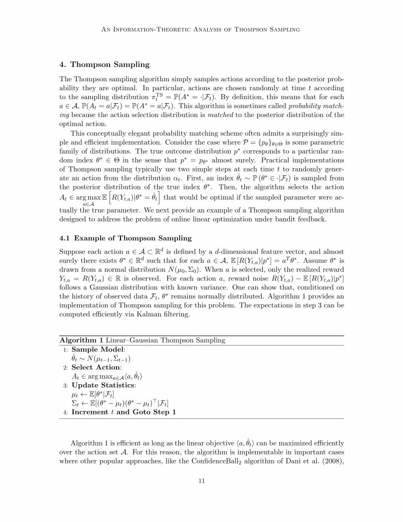
Suppose each action a ∈ A ⊂ Rd is defined by a d-dimensional feature vector, and almostsurely there exists θ∗ ∈ Rd such that for each a ∈ A, E [R(Yt,a)|p∗] = aT θ∗. Assume θ∗ isdrawn from a normal distribution N(µ0,Σ0). When a is selected, only the realized rewardYt,a = R(Yt,a) ∈ R is observed. For each action a, reward noise R(Yt,a) − E [R(Yt,a)|p∗]follows a Gaussian distribution with known variance. One can show that, conditioned onthe history of observed data Ft, θ∗ remains normally distributed. Algorithm 1 provides animplementation of Thompson sampling for this problem. The expectations in step 3 can becomputed efficiently via Kalman filtering.

Algorithm 1 Linear–Gaussian Thompson Sampling

1: Sample Model:θt ∼ N(µt−1,Σt−1)

2: Select Action:At ∈ arg maxa∈A〈a, θt〉

3: Update Statistics:µt ← E[θ∗|Ft]Σt ← E[(θ∗ − µt)(θ∗ − µt)>|Ft]

4: Increment t and Goto Step 1

Algorithm 1 is efficient as long as the linear objective 〈a, θt〉 can be maximized efficientlyover the action set A. For this reason, the algorithm is implementable in important caseswhere other popular approaches, like the ConfidenceBall2 algorithm of Dani et al. (2008),

11

Russo and Van Roy

are computationally intractable. Because the posterior distribution of θ∗ has a closed form,Algorithm 1 is particularly efficient. Even when the posterior distribution is complex, how-ever, one can often generate samples from this distribution using Markov chain Monte Carloalgorithms, enabling efficient implementations of Thompson sampling. A more detailed dis-cussion of the strengths and potential advantages of Thompson sampling can be found inearlier work (Scott, 2010; Chapelle and Li, 2011; Russo and Van Roy, 2014; Gopalan et al.,2014).

5. The Information Ratio and a General Regret Bound

Our analysis will relate the expected regret of Thompson sampling to its expected informa-tion gain: the expected reduction in the entropy of the posterior distribution of A∗. Therelationship between these quantities is characterized by what we call the information ratio,

Γt :=Et [R(Yt,A∗)−R(Yt,At)]

2

It (A∗; (At, Yt,At))

which is the ratio between the square of expected regret and information gain in period t.Recall that, as described in Subsection 3.1, the subscript t on Et and It indicates that thesequantities are evaluated under the posterior measure Pt(·) = P(·|Ft).

Notice that if the information ratio is small, Thompson sampling can only incur largeregret when it is expected to gain a lot of information about which action is optimal. Thissuggests its expected regret is bounded in terms of the maximum amount of informationany algorithm could expect to acquire, which is at most the entropy of the prior distributionof the optimal action. Our next result shows this formally. We provide a general upperbound on the expected regret of Thompson sampling that depends on the time horizon T ,the entropy of the prior distribution of A∗, H(A∗), and any worst–case upper bound on theinformation ratio Γt. In the next section, we will provide bounds on Γt for some of the mostwidely studied classes of online optimization problems.

Proposition 1 For any T ∈ N, if Γt ≤ Γ almost surely for each t ∈ 1, .., T,

E[Regret(T, πTS)

]≤√

ΓH(A∗)T .

Proof Recall that Et[·] = E[·|Ft] and we use It to denote mutual information evaluatedunder the base measure Pt(·) = P(·|Ft). Then,

E[Regret(T, πTS)

] (a)= E

T∑t=1

Et [R(Yt,A∗)−R(Yt,At)] = ET∑t=1

√ΓtIt (A∗; (At, Yt,At))

≤√

Γ

(E

T∑t=1

√It (A∗; (At, Yt,At))

)(b)

≤

√√√√ΓTET∑t=1

It (A∗; (At, Yt,At)),

12


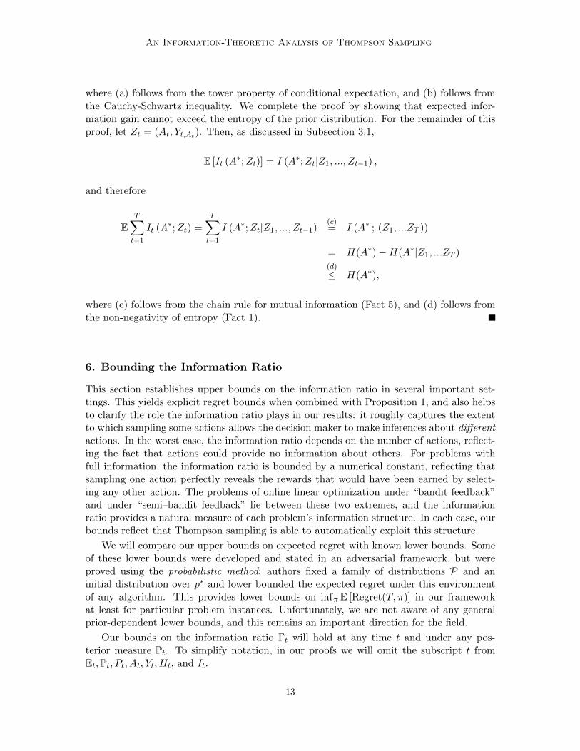
where (a) follows from the tower property of conditional expectation, and (b) follows fromthe Cauchy-Schwartz inequality. We complete the proof by showing that expected infor-mation gain cannot exceed the entropy of the prior distribution. For the remainder of thisproof, let Zt = (At, Yt,At). Then, as discussed in Subsection 3.1,

E [It (A∗;Zt)] = I (A∗;Zt|Z1, ..., Zt−1) ,

and therefore

ET∑t=1

It (A∗;Zt) =

T∑t=1

I (A∗;Zt|Z1, ..., Zt−1)(c)= I (A∗ ; (Z1, ...ZT ))

= H(A∗)−H(A∗|Z1, ...ZT )

(d)

≤ H(A∗),

where (c) follows from the chain rule for mutual information (Fact 5), and (d) follows fromthe non-negativity of entropy (Fact 1).

6. Bounding the Information Ratio

This section establishes upper bounds on the information ratio in several important set-tings. This yields explicit regret bounds when combined with Proposition 1, and also helpsto clarify the role the information ratio plays in our results: it roughly captures the extentto which sampling some actions allows the decision maker to make inferences about differentactions. In the worst case, the information ratio depends on the number of actions, reflect-ing the fact that actions could provide no information about others. For problems withfull information, the information ratio is bounded by a numerical constant, reflecting thatsampling one action perfectly reveals the rewards that would have been earned by select-ing any other action. The problems of online linear optimization under “bandit feedback”and under “semi–bandit feedback” lie between these two extremes, and the informationratio provides a natural measure of each problem’s information structure. In each case, ourbounds reflect that Thompson sampling is able to automatically exploit this structure.

We will compare our upper bounds on expected regret with known lower bounds. Someof these lower bounds were developed and stated in an adversarial framework, but wereproved using the probabilistic method; authors fixed a family of distributions P and aninitial distribution over p∗ and lower bounded the expected regret under this environmentof any algorithm. This provides lower bounds on infπ E [Regret(T, π)] in our frameworkat least for particular problem instances. Unfortunately, we are not aware of any generalprior-dependent lower bounds, and this remains an important direction for the field.

Our bounds on the information ratio Γt will hold at any time t and under any pos-terior measure Pt. To simplify notation, in our proofs we will omit the subscript t fromEt,Pt, Pt, At, Yt, Ht, and It.

13

Russo and Van Roy

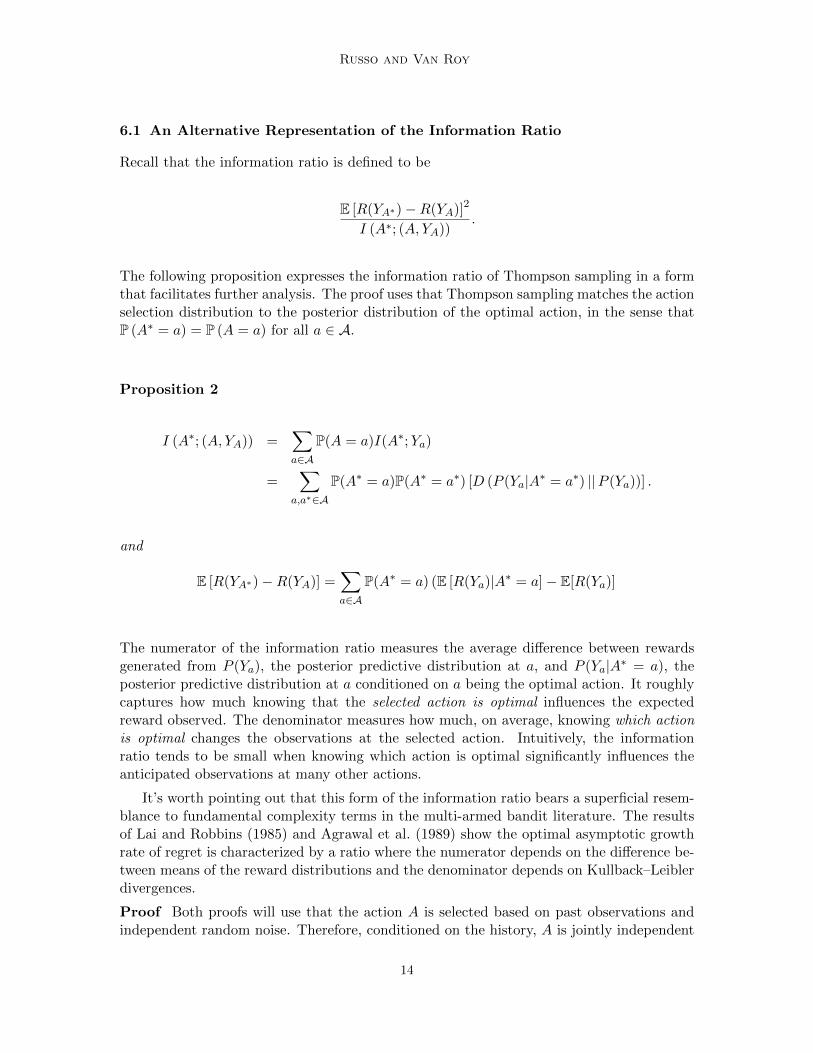
6.1 An Alternative Representation of the Information Ratio

Recall that the information ratio is defined to be

E [R(YA∗)−R(YA)]2

I (A∗; (A, YA)).

The following proposition expresses the information ratio of Thompson sampling in a formthat facilitates further analysis. The proof uses that Thompson sampling matches the actionselection distribution to the posterior distribution of the optimal action, in the sense thatP (A∗ = a) = P (A = a) for all a ∈ A.

Proposition 2

I (A∗; (A, YA)) =∑a∈A

P(A = a)I(A∗;Ya)

=∑

a,a∗∈AP(A∗ = a)P(A∗ = a∗) [D (P (Ya|A∗ = a∗) ||P (Ya))] .

and

E [R(YA∗)−R(YA)] =∑a∈A

P(A∗ = a) (E [R(Ya)|A∗ = a]− E[R(Ya)]

The numerator of the information ratio measures the average difference between rewardsgenerated from P (Ya), the posterior predictive distribution at a, and P (Ya|A∗ = a), theposterior predictive distribution at a conditioned on a being the optimal action. It roughlycaptures how much knowing that the selected action is optimal influences the expectedreward observed. The denominator measures how much, on average, knowing which actionis optimal changes the observations at the selected action. Intuitively, the informationratio tends to be small when knowing which action is optimal significantly influences theanticipated observations at many other actions.

It’s worth pointing out that this form of the information ratio bears a superficial resem-blance to fundamental complexity terms in the multi-armed bandit literature. The resultsof Lai and Robbins (1985) and Agrawal et al. (1989) show the optimal asymptotic growthrate of regret is characterized by a ratio where the numerator depends on the difference be-tween means of the reward distributions and the denominator depends on Kullback–Leiblerdivergences.

Proof Both proofs will use that the action A is selected based on past observations andindependent random noise. Therefore, conditioned on the history, A is jointly independent

14


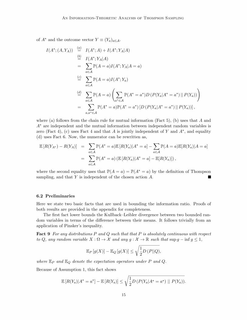
of A∗ and the outcome vector Y ≡ (Ya)a∈A.

I(A∗; (A, YA))(a)= I(A∗;A) + I(A∗;YA|A)

(b)= I(A∗;YA|A)

=∑a∈A

P(A = a)I(A∗;YA|A = a)

(c)=

∑a∈A

P(A = a)I(A∗;Ya)

(d)=

∑a∈A

P(A = a)

(∑a∗∈A

P(A∗ = a∗)D (P (Ya|A∗ = a∗) ||P (Ya))

)=

∑a,a∗∈A

P(A∗ = a)P(A∗ = a∗) [D (P (Ya|A∗ = a∗) ||P (Ya))] ,

where (a) follows from the chain rule for mutual information (Fact 5), (b) uses that A andA∗ are independent and the mutual information between independent random variables iszero (Fact 4), (c) uses Fact 4 and that A is jointly independent of Y and A∗, and equality(d) uses Fact 6. Now, the numerator can be rewritten as,

E [R(YA∗)−R(YA)] =∑a∈A

P(A∗ = a)E [R(Ya)|A∗ = a]−∑a∈A

P(A = a)E[R(Ya)|A = a]

=∑a∈A

P(A∗ = a) (E [R(Ya)|A∗ = a]− E[R(Ya)]) ,

where the second equality uses that P(A = a) = P(A∗ = a) by the definition of Thompsonsampling, and that Y is independent of the chosen action A.

6.2 Preliminaries

Here we state two basic facts that are used in bounding the information ratio. Proofs ofboth results are provided in the appendix for completeness.

The first fact lower bounds the Kullback–Leibler divergence between two bounded ran-dom variables in terms of the difference between their means. It follows trivially from anapplication of Pinsker’s inequality.

Fact 9 For any distributions P and Q such that that P is absolutely continuous with respectto Q, any random variable X : Ω→ X and any g : X → R such that sup g − inf g ≤ 1,

EP [g(X)]− EQ [g(X)] ≤√

1

2D (P ||Q),

where EP and EQ denote the expectation operators under P and Q.

Because of Assumption 1, this fact shows

E [R(Ya)|A∗ = a∗]− E [R(Ya)] ≤√

1

2D (P (Ya|A∗ = a∗) || P (Ya)).

15

Russo and Van Roy

By the Cauchy–Schwartz inequality, for any vector x ∈ Rn,∑

i xi ≤√n‖x‖2. The next

fact provides an analogous result for matrices. For any rank r matrix M ∈ Rn×n withsingular values σ1, ..., σr, let

‖M‖∗ :=r∑i=1

σi, ‖M‖F :=√∑m

k=1

∑nj=1M

2i,j =

√∑ri=1 σ

2i , Trace(M) :=

n∑i=1

Mii,

denote respectively the Nuclear norm, Frobenius norm and trace of M .

Fact 10 For any matrix M ∈ Rk×k,

Trace (M) ≤√

Rank(M)‖M‖F.

6.3 Worst Case Bound

The next proposition provides a bound on the information ratio that holds whenever rewardsare bounded, but that has an explicit dependence on the number of actions. This scalingcannot be improved in general, but we go on to show tighter bounds are possible for problemswith different information structures.

Proposition 3 For any t ∈ N, Γt ≤ |A|/2 almost surely.

Proof We bound the numerator of the information ratio by |A|/2 times its denominator:

E [R(YA∗)−R(YA)]2(a)=

(∑a∈A

P(A∗ = a) (E [R(Ya)|A∗ = a]− E[R(Ya)])

)2

(b)

≤ |A|∑a∈A

P(A∗ = a)2 (E [R(Ya)|A∗ = a]− E[R(Ya)])2

≤ |A|∑

a,a∗∈AP(A∗ = a)P(A∗ = a∗) (E [R(Ya)|A∗ = a∗]− E[R(Ya)])

2

(c)

≤ |A|2

∑a,a∗∈A

P(A∗ = a)P(A∗ = a∗)D (P (Ya|A∗ = a∗) || P (Ya))

(d)=|A|I(A∗; (A, Y ))

2

where (b) follows from the Cauchy–Schwarz inequality, (c) follows from Fact 9, and (a) and(d) follow from Proposition 2.

Combining Proposition 3 with Proposition 1 shows that E[Regret(T, πTS)

]≤√

12 |A|H(A∗)T .

Bubeck and Liu (2013) show E[Regret(T, πTS)

]≤ 14

√|A|T and that this bound is order

optimal, in the sense that for any time horizon T and number of actions |A| there exists aprior distribution over p∗ such that infπ E [Regret(T, π)] ≥ 1

20

√|A|T .

16


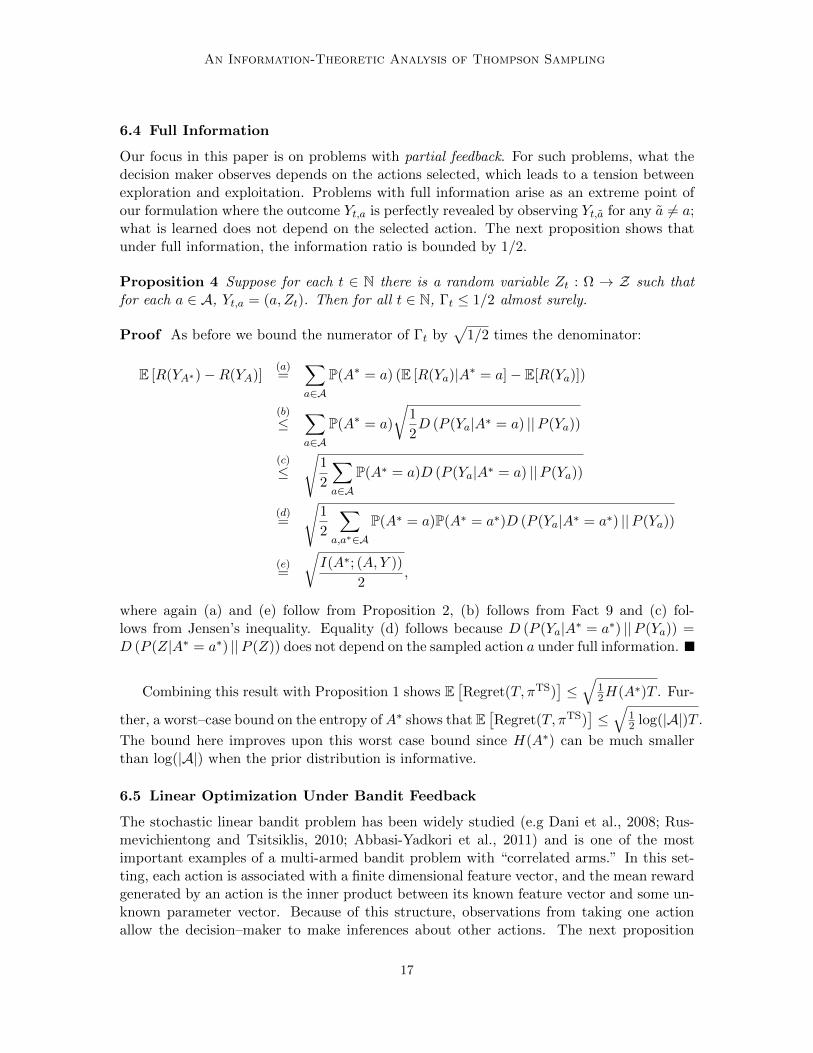
6.4 Full Information

Our focus in this paper is on problems with partial feedback. For such problems, what thedecision maker observes depends on the actions selected, which leads to a tension betweenexploration and exploitation. Problems with full information arise as an extreme point ofour formulation where the outcome Yt,a is perfectly revealed by observing Yt,a for any a 6= a;what is learned does not depend on the selected action. The next proposition shows thatunder full information, the information ratio is bounded by 1/2.

Proposition 4 Suppose for each t ∈ N there is a random variable Zt : Ω → Z such thatfor each a ∈ A, Yt,a = (a, Zt). Then for all t ∈ N, Γt ≤ 1/2 almost surely.

Proof As before we bound the numerator of Γt by√

1/2 times the denominator:

E [R(YA∗)−R(YA)](a)=

∑a∈A

P(A∗ = a) (E [R(Ya)|A∗ = a]− E[R(Ya)])

(b)

≤∑a∈A

P(A∗ = a)

√1

2D (P (Ya|A∗ = a) ||P (Ya))

(c)

≤√

1

2

∑a∈A

P(A∗ = a)D (P (Ya|A∗ = a) ||P (Ya))

(d)=

√1

2

∑a,a∗∈A

P(A∗ = a)P(A∗ = a∗)D (P (Ya|A∗ = a∗) ||P (Ya))

(e)=

√I(A∗; (A, Y ))

2,

where again (a) and (e) follow from Proposition 2, (b) follows from Fact 9 and (c) fol-lows from Jensen’s inequality. Equality (d) follows because D (P (Ya|A∗ = a∗) ||P (Ya)) =D (P (Z|A∗ = a∗) ||P (Z)) does not depend on the sampled action a under full information.

Combining this result with Proposition 1 shows E[Regret(T, πTS)

]≤√

12H(A∗)T . Fur-

ther, a worst–case bound on the entropy ofA∗ shows that E[Regret(T, πTS)

]≤√

12 log(|A|)T .

The bound here improves upon this worst case bound since H(A∗) can be much smallerthan log(|A|) when the prior distribution is informative.

6.5 Linear Optimization Under Bandit Feedback

The stochastic linear bandit problem has been widely studied (e.g Dani et al., 2008; Rus-mevichientong and Tsitsiklis, 2010; Abbasi-Yadkori et al., 2011) and is one of the mostimportant examples of a multi-armed bandit problem with “correlated arms.” In this set-ting, each action is associated with a finite dimensional feature vector, and the mean rewardgenerated by an action is the inner product between its known feature vector and some un-known parameter vector. Because of this structure, observations from taking one actionallow the decision–maker to make inferences about other actions. The next proposition

17

Russo and Van Roy

bounds the information ratio for such problems. Its proof is essentially a generalization ofthe proof of Proposition 3.

Proposition 5 If A ⊂ Rd and for each p ∈ P there exists θp ∈ Rd such that for all a ∈ A

Ey∼pa

[R(y)] = aT θp,

then for all t ∈ N, Γt ≤ d/2 almost surely.

Proof Write A = a1, ..., aK and, to reduce notation, for the remainder of this proof letαi = P(A∗ = ai). Define M ∈ RK×K by

Mi,j =√αiαj (E[R(Yai)|A∗ = aj ]− E[R(Yai)]) ,

for all i, j ∈ 1, ..,K. Then, by Proposition 2,

E [R(YA∗)−R(YA)] =

K∑i=1

αi (E[R(Yai)|A∗ = ai]− E[R(Yai)]) = Trace(M).

Similarly, by Proposition 2,

I(A∗; (A, YA)) =∑i,j

αiαjD (P (Yai |A∗ = aj) ||P (Yai))

(a)

≥ 2∑i,j

αiαj (E[R(Yai)|A∗ = aj ]− E[R(Yai)])2

= 2‖M‖2F,

where inequality (a) uses Fact 9. This shows, by Fact 10, that

E [R(YA∗)−R(YA)]2

I(A∗; (A, YA))≤ Trace(M)2

2‖M‖2F≤ Rank(M)

2.

We now show Rank(M) ≤ d. Define

µ = E [θp∗ ] µj = E [θp∗ |A∗ = aj ] .

Then, by the linearity of the expectation operator,

Mi,j =√αiαj((µ

j − µ)Tai)

and therefore

M =

√α1

(µ1 − µ

)T......√

αK)(µk − µ

)T

[ √α1a1 · · · · · · √αKaK].

18


This shows M is the product of a K by d matrix and a d by K matrix, and hence has rankat most d.

This result shows that E[Regret(T, πTS)

]≤√

12H(A∗)dT ≤

√12 log(|A|)dT for linear ban-

dit problems. Dani et al. (2007) show this bound is order optimal, in the sense that forany time horizon T and dimension d if the actions set is A = 0, 1d, there exists a priordistribution over p∗ such that infπ E [Regret(T, π)] ≥ c0

√log(|A|)dT where c0 is a constant

the is independent of d and T . The bound here improves upon this worst case bound sinceH(A∗) can be much smaller than log(|A|) when the prior distribution is informative.

6.6 Combinatorial Action Sets and “Semi–Bandit” Feedback

To motivate the information structure studied here, consider a simple resource allocationproblem. There are d possible projects, but the decision–maker can allocate resources to atmost m ≤ d of them at a time. At time t, project i ∈ 1, .., d yields a random reward θt,i,and the reward from selecting a subset of projects a ∈ A ⊂ a′ ⊂ 0, 1, ..., d : |a′| ≤ m ism−1

∑i∈A θt,i. In the linear bandit formulation of this problem, upon choosing a subset of

projects a the agent would only observe the overall reward m−1∑

i∈a θt,i. It may be naturalinstead to assume that the outcome of each selected project (θt,i : i ∈ a) is observed. Thistype of observation structure is sometimes called “semi–bandit” feedback (Audibert et al.,2013).

A naive application of Proposition 5 to address this problem would show Γt ≤ d/2. Thenext proposition shows that since the entire parameter vector (θt,i : i ∈ a) is observed uponselecting action a, we can provide an improved bound on the information ratio. The proofof the proposition is provided in the appendix.

Proposition 6 Suppose A ⊂ a ⊂ 0, 1, ..., d : |a| ≤ m, and that there are random vari-ables (θt,i : t ∈ N, i ∈ 1, ..., d) such that

Yt,a = (θt,i : i ∈ a) and R (Yt,a) =1

m

∑i∈a

θt,i.

Assume that the random variables θt,i : i ∈ 1, ..., d are independent conditioned on Ftand θt,i ∈ [−1

2 ,12 ] almost surely for each (t, i). Then for all t ∈ N, Γt ≤ d

2m2 almost surely.

In this problem, there are as many as(dm

)actions, but because Thompson sampling ex-

ploits the structure relating actions to one another, its regret is only polynomial in m andd. In particular, combining Proposition 6 with Proposition 1 shows E

[Regret(T, πTS)

]≤

1m

√dH(A∗)T . Since H(A∗) ≤ log |A| = O(m log( dm)) this also yields a bound of order√

dm log

(dm

)T . As shown by Audibert et al. (2013), the lower bound for this problem is

of order√

dmT , so our bound is order optimal up to a

√log( dm) factor.3 It’s also worth

3. In their formulation, the reward from selecting action a is∑i∈a θt,i, which is m times larger than in our

formulation. The lower bound stated in their paper is therefore of order√mdT . They don’t provide

a complete proof of their result, but note that it follows from standard lower bounds in the banditliterature. In the proof of Theorem 5 in that paper, they construct an example in which the decision

19

Russo and Van Roy

pointing that, although there may be as many as(dm

)actions, the action selection step

of Thompson sampling is computationally efficient whenever the offline decision problemmaxa∈A θ

Ta can be solved efficiently.

7. Conclusion

This paper has provided a new analysis of Thompson sampling based on tools from infor-mation theory. As such, our analysis inherits the simplicity and elegance enjoyed by workin that field. Further, our results apply to a much broader range of information structuresthan those studied in prior work on Thompson sampling. Our analysis leads to regretbounds that highlight the benefits of soft knowledge, quantified in terms of the entropy ofthe optimal-action distribution. Such regret bounds yield insight into how future perfor-mance depends on past observations. This is key to assessing the benefits of exploration,and as such, to the design of more effective schemes that trade off between exploration andexploitation. In forthcoming work, we leverage this insight to produce an algorithm thatoutperforms Thompson sampling.

While our focus has been on providing theoretical guarantees for Thompson sampling,we believe the techniques and quantities used in the analysis may be of broader interest. Ourformulation and notation may be complex, but the proofs themselves essentially follow fromcombining known relations in information theory with the tower property of conditionalexpectation, Jensen’s inequality, and the Cauchy–Schwartz inequality. In addition, theinformation theoretic view taken in this paper may provide a fresh perspective on this classof problems.

Acknowledgments

Daniel Russo is supported by a Burt and Deedee McMurty Stanford Graduate Fellow-ship. This work was supported, in part, by the National Science Foundation under GrantCMMI-0968707. The authors would like to thank the anonymous reviewers for their helpfulcomments.

Appendix A. Proof of Basic Facts

A.1 Proof of Fact 9

This result is a consequence of Pinsker’s inequality, (see Lemma 5.2.8 of Gray (2011)) whichstates that √

1

2D(P ||Q) ≥ ‖P −Q‖TV (7)

maker plays m bandit games in parallel, each with d/m actions. Using that example, and the standardbandit lower bound (see Theorem 3.5 of Bubeck and Cesa-Bianchi (2012)), the agent’s regret from each

component must be at least√

dmT , and hence her overall expected regret is lower bounded by a term of

order m√

dmT =

√mdT .

20


where ‖P −Q‖TV is the total variation distance between P and Q. When Ω is countable,‖P−Q‖TV = 1

2

∑ω |P (ω)−Q(ω)|. More generally, if P andQ are both absolutely continuous

with respect to some base measure µ, then ‖P −Q‖TV = 12

∫Ω |

dPdµ −

dQdµ |dµ, where dP

dµ anddQdµ are the Radon–Nikodym derivatives of P and Q with respect to µ. We now prove Fact9.Proof Choose a base measure µ so that P and Q are absolutely continuous with respect toµ. This is always possible: since P is absolutely continuous with respect to Q by hypothesis,one could always choose this base measure to be Q. Let f(ω) = g(X(ω))− infω′ g(X(ω′))−1/2 so that f : Ω→ [−1/2, 1/2] and f and g(X) differ only by a constant. Then,√

1

2D(P ||Q) ≥ 1

2

∫ ∣∣∣∣dPdµ − dQ

dµ

∣∣∣∣ dµ ≥ 1

2

∫ ∣∣∣∣2(dPdµ − dQ

dµ

)f

∣∣∣∣ dµ≥

∫ (dP

dµ− dQ

dµ

)fdµ

=

∫fdP −

∫fdQ

= EP [g(X)]− EQ[g(X)],

where the first inequality is Pinsker’s inequality.

A.2 Proof of Fact 10

Proof Fix a rank r matrix M ∈ Rk×k with singular values σ1 ≥ ... ≥ σr. By the CauchyShwartz inequality,

‖M‖∗Def=

r∑i=1

σi ≤√r

√√√√ r∑i=1

σ2i

Def=√r‖M‖F . (8)

Now, we show

Trace(M) = Trace

(1

2M +

1

2MT

)(a)

≤∥∥∥∥1

2M +

1

2MT

∥∥∥∥∗

(b)

≤ 1

2‖M‖∗ +

1

2

∥∥MT∥∥∗

(c)= ‖M‖∗

(d)

≤√r‖M‖F .

Here (b) follows from the triangle inequality and the fact that norms are homogeneous ofdegree one. Inequality (c) uses that the singular values of M and MT are the same, andinequality (d) follows from equation (8).

To justify inequality (a), we show that for any symmetric matrix W , Trace(W ) ≤ ‖W‖∗.To see this, let W be a rank r matrix and let σ1 ≥ ... ≥ σr denote its singular val-ues. Since W is symmetric, it has r nonzero real valued eigenvalues λ1, .., λr. If theseare sorted so that |λ1| ≥ ... ≥ |λr| then σi = |λi| for each i ∈ 1, .., r.4 This showsTrace(M) =

∑ri=1 λi ≤

∑ri=1 σi = ‖M‖∗.

4. This fact is stated, for example, in Appendix A.5 of Boyd and Vandenberghe (2004).

21

Russo and Van Roy

Appendix B. Proof of Proposition 6

The proof relies on the following lemma, which lower bounds the information gain due toselecting an action a. The proof is provided below, and relies on the chain–rule of Kullback–Leibler divergence.

Lemma 1 Under the conditions of Proposition 6, for any a ∈ A,

I(A∗;Ya) ≥ 2∑i∈a

P(i ∈ A∗) (E [θi|i ∈ A∗]− E [θi])2

Proof In the proof of this lemma, for any i ∈ a we let θ<i = (θj : j < i, j ∈ a). Sincea ∈ A is fixed throughout this proof, we do not display the dependence of θ<i on a. Recallthat by Fact 6,

I(A∗;Ya) =∑a∗∈A

P(A∗ = a∗)D (P (Ya|A∗ = a∗) ||P (Ya)) .

where here,

D (P (Ya|A∗ = a∗) ||P (Ya)) = D (P ((θi : i ∈ a)|A∗ = a∗) || P ((θi : i ∈ a)))

(a)=

∑i∈a

E[D (P (θi|A∗ = a∗, θ<i) || P (θi|θ<i))

∣∣∣∣A∗ = a∗]

(b)

≥ 2∑i∈a

E[(E [θi|A∗ = a∗, θ<i]− E [θi|θ<i])2

∣∣∣∣A∗ = a∗]

(c)= 2

∑i∈a

E[(E [θi|A∗ = a∗, θ<i]− E [θi])

2

∣∣∣∣A∗ = a∗]

(d)

≥ 2∑i∈a

(E [θi|A∗ = a∗]− E [θi])2 .

Equality (a) follows from the chain rule of Kullback–Leibler divergence, (b) follows fromFact 9, (c) follows from the assumption that (θi : 1 ≤ i ≤ d) are independent conditioned onany history of observations, and (d) follows from Jensen’s inequality and the tower property

22


of conditional expectation. Now, we can show

I(A∗;Ya) ≥ 2∑i∈a

∑a∗∈A

P(A∗ = a∗) (E [θi|A∗ = a∗]− E [θi])2

= 2∑i∈a

P(i ∈ A∗)∑a∗∈A

P(A∗ = a∗)

P(i ∈ A∗)(E [θi|A∗ = a∗]− E [θi])

2

≥ 2∑i∈a

P(i ∈ A∗)∑

a∗:i∈a∗

P(A∗ = a∗)

P(i ∈ A∗)(E [θi|A∗ = a∗]− E [θi])

2

= 2∑i∈a

P(i ∈ A∗)∑

a∗:i∈a∗P(A∗ = a∗|i ∈ A∗) (E [θi|A∗ = a∗]− E [θi])

2

(e)

≥ 2∑i∈a

P(i ∈ A∗)

( ∑a∗:i∈a∗

P(A∗ = a∗|i ∈ A∗) (E [θi|A∗ = a∗]− E [θi])

)2

(f)= 2

∑i∈a

P(i ∈ A∗) (E [θi|i ∈ A∗]− E [θi])2 ,

where (e) and (f) follow from Jensen’s inequality and the tower property of conditionalexpectation, respectively.

Lemma 2 Under the conditions of Proposition 6,

I(A∗; (A, YA)) ≥ 2d∑i=1

P(i ∈ A∗)2 (E [θi|i ∈ A∗]− E [θi])2 .

Proof By Lemma 1 and the tower property of conditional expectation,

I(A∗; (A;YA)) = P(A∗ = a)I(A∗;Ya)

≥ 2∑a∈A

P(A∗ = a)

[∑i∈a

P(i ∈ A∗) (E [θi|i ∈ A∗]− E [θi])2

]

= 2d∑i=1

∑a:i∈a

P(A∗ = a)(P(i ∈ A∗) (E [θi|i ∈ A∗]− E [θi])

2)

= 2

d∑i=1

P(i ∈ A∗)2 (E [θi|i ∈ A∗]− E [θi])2 .

Now, we complete the proof of Proposition 6.

23

Russo and Van Roy

Proof The proof establishes that the numerator of the information ratio is less than d/2m2

times its denominator:

mE[R(YA∗)−R(YA)] = E∑i∈A∗

θi − E∑i∈A

θi

=d∑i=1

P(i ∈ A∗)E[θi|i ∈ A∗]−d∑i=1

P(i ∈ A)E[θi|i ∈ A]

=

d∑i=1

P(i ∈ A∗) (E[θi|i ∈ A∗]− E[θi])

≤√d

√√√√ d∑i=1

P(i ∈ A∗)2 (E[θi|i ∈ A∗]− E[θi])2

≤√dI(A∗; (A, YA))

2.

Appendix C. Proof of Fact 6

We could not find a reference that proves Fact 6 in a general setting, and will thereforeprovide a proof here.

Consider random variables X : Ω → X and Y : Ω → Y where X is assumed to be afinite set but Y is a general random variable. We show

I(X;Y ) =∑x∈X

P (X = x)D (P (Y ∈ ·|X = x) ||P (Y ∈ ·)) .

When Y has finite support this result follows easily by using that P(X = x, Y = y) =P(X = x)P(Y = y|X = x). For an extension to general random variables Y we followchapter 5 of Gray (2011).

The extension follows by considering quantized versions of the random variable Y . Fora finite partition Q = Qi ⊂ Yi∈I , we denote by YQ the quantization of Y defined so thatYQ(ω) = i if and only if Y (ω) ∈ Qi. As shown in Gray (2011), for two probability measuresP1 and P2 on (Ω,F),

D (P1(Y ∈ ·)||P2(Y ∈ ·)) = supQD (P1(YQ ∈ ·)||P2(YQ ∈ ·)) , (9)

where the supremum is taken over all finite partitions of Y, and whenever Q is a refinementof Q,

D(P1(YQ ∈ ·)||P2(YQ ∈ ·)

)≥ D (P1(YQ ∈ ·)||P2(YQ ∈ ·)) . (10)

Since I(X;Y ) = D (P(X ∈ ·, Y ∈ ·) ||P(X ∈ ·)P(Y ∈ ·)) these properties also apply to I(X;YQ).Now, for each x ∈ X we can introduce a sequence of successively refined partitions (Qxn)n∈N

24


so that

D (P (Y ∈ ·|X = x) ||P (Y ∈ ·)) = limn→∞

D(P(YQxn ∈ ·|X = x

)||P(YQxn ∈ ·

))= sup

QD (P (YQ ∈ ·|X = x) ||P (YQ ∈ ·)) .

Let the finite partition Qn denote the refinement of the partitions Qxnx∈X . That is, foreach x, every set in Qxn can be written as the union of sets in Qn. Then,

I(X;Y ) ≥ limn→∞

I(X;YQn)

= limn→∞

∑x∈X

P (X = x)D (P (YQn ∈ ·|X = x) ||P (YQn ∈ ·))

≥ limn→∞

∑x∈X

P (X = x)D(P(YQxn ∈ ·|X = x

)||P(YQxn ∈ ·

))=

∑x∈X

P (X = x)D (P (Y ∈ ·|X = x) ||P (Y ∈ ·))

=∑x∈X

P (X = x) supQx

D (P (YQx ∈ ·|X = x) ||P (YQx ∈ ·))

≥ supQ

∑x∈X

P (X = x)D (P (YQ ∈ ·|X = x) ||P (YQ ∈ ·))

= supQI(X;YQ) = I(X;Y ),

hence the inequalities above are equalities and our claim is established.

Appendix D. Technical Extensions

D.1 Infinite Action Spaces

In this section, we discuss how to extend our results to problems where the action spaceis infinite. For concreteness, we will focus on linear optimization problems. Specifically,throughout this section our focus is on problems where A ⊂ Rd and for each p ∈ P there issome θp ∈ Θ ⊂ Rd such that for all a ∈ A

Ey∼pa

[R(y)] = aT θp.

We assume further that there is a fixed constant c ∈ R such that supa∈A ‖a‖2 ≤ c andsupθ∈Θ ‖θ‖2 ≤ c. Because A is compact, it can be extremely well approximated by a finiteset. In particular, we can choose a finite cover Aε ⊂ A with log |Aε| = O(d log(dc/ε) suchthat for every a ∈ A, mina∈Aε ‖a− a‖2 ≤ ε. By the Cauchy-Schwartz inequality, this impliesthat | (a− a)T θP | ≤ cε for every θP .

We introduce a quantization A∗Q of the random variable A∗. A∗Q is supported only onthe set Aε, but satisfies ‖A∗(ω)−A∗Q(ω)‖2 ≤ ε for each ω ∈ Ω.

25

Russo and Van Roy

Consider a variant of Thompson sampling that randomizes according to the distribution

of A∗Q. That is, for each a ∈ Aε, P (At = a|Ft) = P(A∗Q = a|Ft

). Then, our analysis shows,

ET∑t=1

[R(Yt,A∗)−R(Yt,At)] = ET∑t=1

[R(Yt,A∗)−R(Yt,A∗Q)

]+ E

T∑t=1

[R(Yt,A∗Q)−R(Yt,At)

]≤ εT +

√dTH

(A∗Q

).

This new bound depends on the time horizon T , the dimension d of the linear model, theentropy of the prior distribution of the quantized random variable A∗Q and the discretization

error εT . Since H(A∗Q) ≤ log (|Aε|), by choosing ε = (cT )−1 and choosing a finite cover

with log (|Aε|) = O(d log(dcT )) we attain a regret bound of order d√T log(dcT ). Note that

for d ≤ T , this bound is of order d√T log(cT ), but for d > T ≥ 1, we have a trivial regret

bound of T <√dT .

Here, for simplicity, we have considered a variant of Thompson sampling that randomizesaccording to the posterior distribution of the quantized random variable A∗Q. However, witha somewhat more careful analysis, one can provide a similar result for an algorithm thatrandomizes according to the posterior distribution of A∗.

D.2 Unbounded Noise

In this section we relax Assumption 1, which requires that reward distributions are uniformlybounded. This assumption is required for Fact 9 to hold, but otherwise was never used inour analysis. Here, we show that an analogue to Fact 9 holds in the more general settingwhere reward distributions are sub–Gaussian. This yields more general regret bounds.

A random variable is sub–Gaussian if its moment generating function is dominated bythat of a Gaussian random variable. Gaussian random variables are sub–Gaussian, as arereal-valued random varaibles with bounded support.

Definition 1 Fix a deterministic constant σ ∈ R. A real–valued random variable X is σsub–Gaussian if for all λ ∈ R

E [expλX] ≤ expλ2σ2/2.

More generally X is σ sub–Gaussian conditional on a sigma-algebra G ⊂ F if for all λ ∈ R,

E [expλX|G] ≤ expλ2σ2/2

almost surely.

The next lemma extends Fact 9 to sub-Gaussian random variables.

Lemma 3 Suppose there is a Ft measurable random variable σ such that for each a ∈ A,R(Yt,a)) is σ sub-Gaussian conditional on Ft. Then for every a, a∗ ∈ A

Et[R(Yt,a)|A∗ = a∗]− Et[R(Yt,a)] ≤ σ√

2D (Pt(Yt,a|A∗ = a∗) ||Pt(Yt,a)),

almost surely.

26


Using this Lemma in place of Fact 9 in our analysis leads to the following corollary.

Corollary 1 Fix a deterministic constant σ ∈ R. Suppose that conditioned on Ft, R(Yt,a)−E [R(Yt,a|Ft] is σ sub–Gaussian. Then

Γt ≤ 2|A|σ2

almost surely for each t ∈ N. Furthermore, Γt ≤ 2σ2 under the conditions of Proposition4, Γt ≤ 2dσ2 under the conditions of Proposition 5, and Γt ≤ 2dσ2

m2 under the conditions ofProposition 6.

It’s worth highlighting two cases under which the conditions of Corollary 1 are satisfied.The first is a setting with a Gaussian prior and Guassian reward noise. The second case iswhen under any model p ∈ P expected rewards lie in a bounded interval and reward noiseis sub–Gaussian.

1. Suppose that for each a ∈ A, R(Yt,a) follows a Guassian distribution with vari-ance less than σ2, Yt,a = R(Yt,a) and, reward noise R(Yt,a) − E[R(Yt,a)|p∗] is Gaus-sian with known variance. Then, the posterior predictive distribution of R(Yt,a),P (R(Yt,a) ∈ ·|Ft) is Gaussian with variance less than σ2 for each a ∈ A and t ∈ N.

2. Fix constants C ∈ R and σ ∈ R. Suppose that almost surely E [R(Yt,a)|p∗] ∈[−C

2 , C2]

and reward noise is R(Yt,a)− E [R(Yt,a)|p∗] is σ sub–Gaussian. Then, conditioned onthe history, R(Yt,a)− E [R(Yt,a)|Ft] is

√C2 + σ2 sub-Gaussian almost surely.

The first case relies on the fact that E[R(Yt,a)|p∗] is C–sub-Gaussain, as well as the followingfact about sub-Gaussian random variables.

Fact 11 Consider random variables (X1, ..., XK). If for each Xi there is a deterministic

σi such that Xi is σi sub–Gaussian conditional on X1, .., Xi−1, then∑K

i=1Xi is√∑K

i=1 σ2i

sub-Gaussian.

Proof For any λ ∈ R,

E

[expλ

K∑i=1

Xi

]= E

[K∏i=1

expλXi

]= E

[K∏i=1

E[expλXi

∣∣∣∣X1, ..Xi−1

]]

≤K∏i=1

exp

λ2σ2

i

2

= exp

λ2(∑

i σ2i )

2

.

The proof of Lemma 3 relies on the following property of Kullback–Leibler divergence.

Fact 12 (Variational form of KL–Divergence given in Theorem 5.2.1 of Gray (2011)) Fixtwo probability distributions P and Q such that P is absolutely continuous with respect toQ. Then,

D(P ||Q) = supXEP [X]− logEQ [expX] ,

where EP and EQ denote the expectation operator under P and Q respectively, and thesupremum is taken over all real valued random variables X such that EP [X] is well definedand EQ [expX] <∞.

27

Russo and Van Roy

We now show that Lemma 3 follows from the variational form of KL–Divergence.Proof Define the random variable X = R (Yt,a) − Et [R (Yt,a)]. Then, for abitrary λ ∈ R,applying Fact 12 to λX yields

D (Pt (Yt,a|A∗ = a∗) ||Pt(Yt,a)) ≥ λEt [X|A∗ = a∗]− logEt [expλX]= λ (Et[R (Yt,a) |A∗ = a∗]− Et [R (Yt,a)])− logE [expλX|Ft]≥ λ (Et[R (Yt,a) |A∗ = a∗]− Et [R (Yt,a)])− (λ2σ2/2).

Maximizing over λ yields the result.

References

Y. Abbasi-Yadkori, D. Pal, and C. Szepesvari. Improved algorithms for linear stochasticbandits. Advances in Neural Information Processing Systems, 24, 2011.

R. Agrawal, D. Teneketzis, and V. Anantharam. Asymptotically efficient adaptive allocationschemes for controlled iid processes: Finite parameter space. IEEE Transactions onAutomatic Control, 34(3), 1989.

S. Agrawal and N. Goyal. Analysis of Thompson sampling for the multi-armed banditproblem. In Proceedings of the 21st Annual Conference on Learning Theory, 2012.

S. Agrawal and N. Goyal. Further optimal regret bounds for thompson sampling. In Pro-ceedings of the Sixteenth International Conference on Artificial Intelligence and Statistics,pages 99–107, 2013a.

S. Agrawal and N. Goyal. Thompson sampling for contextual bandits with linear payoffs. InProceedings of the 30th International Conference on Machine Learning, pages 127–135,2013b.

J.-Y. Audibert, S. Bubeck, and G. Lugosi. Regret in online combinatorial optimization.Mathematics of Operations Research, 39(1):31–45, 2013.

P. Auer, N. Cesa-Bianchi, and P. Fischer. Finite-time analysis of the multiarmed banditproblem. Machine learning, 47(2):235–256, 2002.

S.P. Boyd and L. Vandenberghe. Convex optimization. Cambridge university press, 2004.

S. Bubeck and N. Cesa-Bianchi. Regret analysis of stochastic and nonstochastic multi-armedbandit problems. Foundations and trends in machine learning, 5(1):1–122, 2012.

S. Bubeck and C.-Y. Liu. Prior-free and prior-dependent regret bounds for Thompsonsampling. In Advances in Neural Information Processing Systems, 2013.

O. Chapelle and L. Li. An empirical evaluation of Thompson sampling. In Neural Infor-mation Processing Systems (NIPS), 2011.

T.M. Cover and J.A. Thomas. Elements of information theory. John Wiley & Sons, 2012.

28


V. Dani, S.M. Kakade, and T.P. Hayes. The price of bandit information for online opti-mization. In Advances in Neural Information Processing Systems, pages 345–352, 2007.

V. Dani, T.P. Hayes, and S.M. Kakade. Stochastic linear optimization under bandit feed-back. In Proceedings of the 21st Annual Conference on Learning Theory, pages 355–366,2008.

J. Gittins, K. Glazebrook, and R. Weber. Multi-armed bandit allocation indices. John Wiley& Sons, Ltd, 2011. ISBN 9780470980033.

A. Gopalan, S. Mannor, and Y. Mansour. Thompson sampling for complex online problems.In Proceedings of the 31st International Conference on Machine Learning, pages 100–108,2014.

T. Graepel, J.Q. Candela, T. Borchert, and R. Herbrich. Web-scale Bayesian click-throughrate prediction for sponsored search advertising in Microsoft’s Bing search engine. InProceedings of the 27th International Conference on Machine Learning, pages 13–20,2010.

R.M. Gray. Entropy and information theory. Springer, 2011.

E. Kauffmann, N. Korda, and R. Munos. Thompson sampling: an asymptotically optimalfinite time analysis. In International Conference on Algorithmic Learning Theory, 2012.

N. Korda, E. Kaufmann, and R. Munos. Thompson sampling for one-dimensional exponen-tial family bandits. In Advances in Neural Information Processing Systems, 2013.

T.L. Lai and H. Robbins. Asymptotically efficient adaptive allocation rules. Advances inapplied mathematics, 6(1):4–22, 1985.

L. Li. Generalized Thompson sampling for contextual bandits. arXiv preprintarXiv:1310.7163, 2013.

B.C. May, N. Korda, A. Lee, and D.S. Leslie. Optimistic Bayesian sampling in contextual-bandit problems. The Journal of Machine Learning Research, 98888:2069–2106, 2012.

P. Rusmevichientong and J.N. Tsitsiklis. Linearly parameterized bandits. Mathematics ofOperations Research, 35(2):395–411, 2010.

D. Russo and B. Van Roy. Learning to optimize via posterior sampling. Mathematics ofOperations Research, 2014. URL http://dx.doi.org/10.1287/moor.2014.0650.

I.O. Ryzhov, W.B. Powell, and P.I. Frazier. The knowledge gradient algorithm for a generalclass of online learning problems. Operations Research, 60(1):180–195, 2012.

S.L. Scott. A modern Bayesian look at the multi-armed bandit. Applied Stochastic Modelsin Business and Industry, 26(6):639–658, 2010.

S.L. Scott. Overview of content experiments: Multi-armed bandit experiments, 2014. URLhttps://support.google.com/analytics/answer/2844870?hl=en. [Online; accessed9-February-2014].

29

Russo and Van Roy

N. Srinivas, A. Krause, S.M. Kakade, and M. Seeger. Information-theoretic regret bounds forGaussian process optimization in the bandit setting. IEEE Transactions on InformationTheory, 58(5):3250 –3265, 2012.

L. Tang, R. Rosales, A. Singh, and D. Agarwal. Automatic ad format selection via contex-tual bandits. In Proceedings of the 22nd ACM international conference on Conference oninformation & knowledge management, pages 1587–1594. ACM, 2013.

W.R. Thompson. On the likelihood that one unknown probability exceeds another in viewof the evidence of two samples. Biometrika, 25(3/4):285–294, 1933.

30

an information-theoretic analysis of thompson...

Documents