an inverse modelling approach to estimate the hygric...
TRANSCRIPT

Accepted Manuscript
An inverse modelling approach to estimate the hygric parameters of clay-basedmasonry during a moisture buffer value test
Samuel Dubois, F.R.I.A Grant holder, Ph.D Student Fionn McGregor, BRE CICM,Ph.D Student Frédéric Lebeau, Professor Arnaud Evrard, PhD Andrew Heath,Associate Professor
PII: S0360-1323(14)00210-8
DOI: 10.1016/j.buildenv.2014.06.018
Reference: BAE 3750
To appear in: Building and Environment
Received Date: 17 February 2014
Revised Date: 20 June 2014
Accepted Date: 21 June 2014
Please cite this article as: Dubois S, McGregor F, Lebeau F, Evrard A, Heath A, An inverse modellingapproach to estimate the hygric parameters of clay-based masonry during a moisture buffer value test,Building and Environment (2014), doi: 10.1016/j.buildenv.2014.06.018.
This is a PDF file of an unedited manuscript that has been accepted for publication. As a service toour customers we are providing this early version of the manuscript. The manuscript will undergocopyediting, typesetting, and review of the resulting proof before it is published in its final form. Pleasenote that during the production process errors may be discovered which could affect the content, and alllegal disclaimers that apply to the journal pertain.

MANUSCRIP
T
ACCEPTED
ACCEPTED MANUSCRIPTHighlights
• The hygric behaviour of two clay samples is modelled with finite-element method • Moisture transfer parameters are estimated with an inverse modelling approach • Estimated parameters are compared to their equivalents measured in steady-state • The MBV test allows to retrieve several parameters values • The inverse modelling offers a more realistic description of parameters

MANUSCRIP
T
ACCEPTED
ACCEPTED MANUSCRIPT
An inverse modelling approach to estimate the hygric parameters of clay-based masonry during a moisture buffer value test Samuel DUBOIS* Ph.D Student, F.R.I.A Grant holder, Dept. of environmental sciences and technologies, Gembloux Agro-Bio Tech, University of Liege, Belgium [email protected] Fionn McGregor PhD Student, BRE CICM, Dept. of Architecture and Civil engineering, University of Bath, UK [email protected] Frédéric LEBEAU Professor, Dept. of environmental sciences and technologies, Gembloux Agro-Bio Tech, University of Liege, Belgium [email protected] Arnaud EVRARD PhD, Architecture et Climat, Université Catholique de Louvain, Belgium [email protected] Andrew HEATH Associate Professor, Dept. of Architecture and Civil engineering, University of Bath, UK [email protected] *Corresponding author Address: Dept. of environmental sciences and technologies, Gembloux Agro-Bio Tech, 2 Passage des déportés, 5030 Gembloux, Belgium Tel: +32 496 96 52 84
ABSTRACT:
This paper presents an inverse modelling approach for parameter estimation of a model dedicated to the description of moisture mass transfer in porous hygroscopic building materials. The hygric behaviour of unfired clay-based masonry samples is specifically studied here and the Moisture Buffer Value (MBV) protocol is proposed as a data source from which it is possible to estimate several parameters at once. Those include materials properties and experimental parameters. For this purpose, the mass of two clay samples with different compositions is continuously monitored during several consecutive humidity cycles in isothermal conditions. Independently of these dynamic experimental tests, their moisture storage and transport parameters are measured with standard steady-state methods.
A simple moisture transfer model developed in COMSOL Multiphysics is used to predict the moisture uptake/release behaviour during the MBV tests. The set of model parameters values that minimizes the difference between simulated and experimental results is then automatically estimated using an inverse modelling algorithm based on Bayesian techniques. For materials properties, the optimized parameters values are compared to values that were experimentally measured in steady state. And because a precise understanding of parameters is needed to assess the confidence in the inverse modelling results, a sensitivity analysis of the model is also provided.
Keywords: Moisture Buffer Value, Clay, HAM Modelling, Parameter estimation, MCMC, DREAM

MANUSCRIP
T
ACCEPTED
ACCEPTED MANUSCRIPT1. INTRODUCTION
Clay has been used as a construction material since man has started building. In 2012 UNESCO released
an inventory of Earth construction heritage sites [1]. It shows the immense legacy of earth construction
and earth architecture around the world. These sites demonstrate how durable this material can be. In
modern times earth has to compete with materials such as concrete and due to its natural variability, earth
is often considered as a primitive material not fit for modern construction. However, earth based masonry
and renders have many qualities that are becoming more and more important in the context of global
climate change and the challenge to reduce carbon emissions. The choice of using earth as a construction
material varies depending on the economical situation of a country. In developing countries earth is a
cheap material that can often be sourced close to the building site making it the first choice for economical
reasons. In richer industrialised countries, earth is chosen for its sustainable, highly hygroscopic and
aesthetic qualities [2].
Clay-based materials show high moisture storage capacity through surface adsorption and capillary
condensation effects in the hygroscopic domain. Such phenomena coupled with moisture transport inside
the porous structure are stated to offer a regulation capacity of the indoor air humidity [3], improving
comfort for occupants [4-6]. One way to quantify this regulation behaviour is to evaluate the moisture
buffer capacity, i.e. the moisture exchange capacity under a dynamic exposure to ambient relative
humidity (RH) cycle. The relative humidity variations can be caused either by temperature change of the
ambient air or through changing the amount of moisture in it.
The NORDTEST project [7] has been one of the first attempts to find a consensus for an experimental
protocol able to adequately characterize the buffer capacity through the definition of a global parameter
called the Moisture Buffer Value (MBV). Beside the direct humidity regulation that is evaluated by the
MBV at material scale, the buffer performance of hygroscopic materials also causes latent heat effects
whose impact on energy balance is only partially assessed [8].
Along with the will to characterize porous hygroscopic and capillary materials experimentally, the
modelling of their behaviour has progressed substantially in the last decades [9-12]. Indeed, Heat Air and
Moisture (HAM) models which deal with detailed hygrothermal analysis of porous materials have
MANUSCRIP
T
ACCEPTED
ACCEPTED MANUSCRIPTimproved in accuracy through the development of computer power and a better knowledge of the involved
phenomena. Many HAM computer models and associated software have been developed for building
applications and some have been commercialized [13, 14]. The main difference between the models is in
the description of the moisture flows that can have several levels of complexity, ranging from diffusivity
models using moisture content as driving potential to conductivity models using the actual thermodynamic
driving potential and separated liquid and vapour flows [15]. All these models rely on material and
boundary condition parameters, most of them being time consuming to obtain.
The computation of temperature and moisture content fields in building materials, from the known
parameters and boundary conditions forms a direct HAM problem [16]. This approach is the most common
in Building Physics, where the aim is often to predict the behaviour of material assemblies under various
climatic solicitations. The validity of such approaches relies on the quality of characterization for the
hygrothermal properties of the material. In contrast to direct modelling process, there exist several
methods that allow parameter estimation from temperature and moisture content field measurements,
which establishes a new kind of inverse HAM problem. Among inverse modelling methods, the Bayesian
approaches are becoming more and more popular in environmental models. In Bayesian optimization,
parameters are not unknowns with a single value to determine, but stochastic variables whose distributions
have to be specified. The distribution given before estimation is called 'a priori' and the distribution given
after integration of the experimental data is called 'a posteriori'. Historically, the emergence of the Markov
Chain Monte Carlo (MCMC) simulations with the Random Walk Metropolis algorithm as first widely
used approach [17] have greatly simplified the estimation of posterior distribution of parameters. Recently,
Ter Braak [18] developed the Differential Evolution-Markov Chain (DE-MC) method, able to run several
Markov chains in parallel with a so called 'genetic' algorithm for the sampling process, improving the
parameter space exploration efficiency. The Differential Evolution Adaptive Metropolis (DREAM)
algorithm [19, 20] is an evolution of the DE-MC, able to automatically tune the scale and orientation of
the proposed parameter distributions (i.e. self-adaptive randomized subspace sampling) during the
evolution towards posterior distribution. A good review about Bayesian approaches and inverse modelling
algorithms evolution can be found in [21].
The goal of this paper is to illustrate the use of a MCMC sampler to estimate the parameters of a HAM
MANUSCRIP
T
ACCEPTED
ACCEPTED MANUSCRIPTmodel in an inverse modelling problem. For this purpose, we propose to study the applicability of the
MBV protocol as the source of experimental data to estimate hygric properties of porous construction
materials. Specifically, the mass variation of different clay-based samples is measured experimentally
during a MBV test. In parallel, their moisture storage and transport properties are measured in steady-state
conditions. The DREAM algorithm is then coupled to a simplified moisture transfer model which
simulates the moisture exchange of samples. The parameters sampling process consists in automatically
tuning the HAM model in order to match experimental mass variation by testing various combinations of
parameters values and evaluating the resulting model efficiency. Eventually, the inverse modelling
approach can propose a 'best parameters set' which minimizes the difference between the simulated and
the measured moisture uptake/release of sample. Four parameters are estimated in this paper; two are
directly related to the material and two others linked to experimental conditions. For the first category, the
best estimated parameters resulting from the inverse modelling approach can be compared to their
corresponding value measured in steady-state.
The questions arising from this study are: (1) how the different model parameters interact during the MBV
cycle, with possible correlations; (2) is it reliable to use this single dynamic experiment to retrieve several
parameters at once with the inverse modelling method; (3) do the dynamic conditions of the MBV test
offer a more 'realistic' configuration for material properties assessment?
2. THE MOISTURE BUFFER VALUE
The need for a standardized parameter to characterize the moisture buffering capacity of materials led to
the definition of the Moisture Buffer Value (MBV) during the NORDTEST project [4] together with the
proposal of a dynamic experimental protocol for materials classification. The practical MBV is defined as
:‘‘the amount of water that is transported in or out of a material per open surface area, during a certain
period of time, when it is subjected to variations in relative humidity of the surrounding air’’ [7].
Concretely, the samples are subjected to cyclic step changes in relative humidity (RH) at a constant
temperature of 23°� and are weighted regularly. The cycle is composed by moisture uptake during 8
hours at high RH followed by moisture release 16 hours at low RH and is repeated until constant mass
MANUSCRIP
T
ACCEPTED
ACCEPTED MANUSCRIPTvariation between 2 consecutive cycles is reached. The practical MBV in ��/( ∙ % �) is then given
by Eq.1.
������������ = ∆� ∙ ∆ � (1)
where ∆ is the mass variation during the 8 hours absorption phase or the 16 hours desorption phase in
one complete cycle, �() is the total exchange surface and ∆ � is the difference between the high and
low relative humidity of the cycle. This experimental value is a direct measurement of the amount of
moisture transported to and from the material for the given exposure cycle. In the original protocol, the
cycle is fixed to a 75/33%RH scheme.
A theoretical value of the MBV, called ��������, can be computed analytically using semi-infinite solid
theory and Fourier series without transfer resistance at exchange surface. There is always a disagreement
between measured and analytically calculated due to the dynamic nature of the experimental protocol, the
film resistance on specimen exchange surface and deviations from the typical step transitions . However is
has been shown in McGregor et al. [22] that a good agreement can be found between measured and
calculated MBV when reducing the film resistance in the dynamic test and improving the precision of the
steady state measured properties.
3. MATERIALS AND METHODS
3.1 Samples
Two different soils were used for the experimental measurement. The Gr soil is a natural soil extracted
from the Wealden clay group in the UK. The natural soil had high clay content, so 50% by weight of fine
builders sand was added. The final particle size distribution consisted of 18% of clay, 24% of silt and 58%
of sand. The Mt is a manufactured soil; it was prepared with 10% of a commercial bentonite, 15% of
kaolin clay, 20% of silt and 55% of sand.
The tested sample blocs have all three a cylindrical shape and a nominal height of 3cm, which is stated
sufficient given the theoretical moisture penetration depth during the MBV experiment. Lateral and back
faces are sealed from water exchange with aluminium tape providing one-dimensional conditions. Table 1
gives the general physical properties of the samples including their volume, true exchange surface area

MANUSCRIP
T
ACCEPTED
ACCEPTED MANUSCRIPTand dry density.
Table 1 Properties of the tested samples
Volume of sample Exchange surface area Dry density � ³ ² !"/ ³
Gr8 21.92 0.0078 2010 Mt9 24.06 0.008 1860
The vapour resistance factors of the two samples were determined by the wet cup method described by the
ISO 12572 Standard. Samples are sealed on the top of a cup containing potassium nitrate solution. The cup
is placed in a chamber at 50%HR and 23°C, giving typically 94±0.60%HR in the air layer above the salt
solution. The processed results give a value of $ = 8.8 for Gr8 sample and 8.3 for Mt9 sample.
The moisture storage curves were determined by a Dynamic Vapour Sorption (DVS) system. The DVS
equipment precisely records the mass of a sample of up to 4g in varying RH conditions. The sorption
isotherms were precisely recorded up to 95%RH within 10 days. Above 95%RH the samples need much
longer to reach Equilibrium Moisture Content (EMC) and therefore the equilibrium was not expected to be
reached at these levels but this is not considered a limitation for this study as 95%RH is above the RH
level from all tests. Once the adsorption curve measurement is finished, the DVS apparatus initiates the
reverse cycle to obtain the experimental points of the desorption curve. All equilibrium moisture content
values are expressed as variable %(�� ∙ ��&'). Fig. 1 shows the DVS curves for the two tested materials.
Fig.1 Moisture storage curves
It can be observed that absorption curves only start to rise steeply from around 80% due to the increase of
MANUSCRIP
T
ACCEPTED
ACCEPTED MANUSCRIPTcapillary condensation effects. As a consequence, it is assumed that hysteresis phenomena are negligible
during the MBV experiments performed later and only absorption curves will be considered. Indeed, the
chosen relative humidity cycle imposed on samples is 16hrs at 50% and 8hrs at 85%. A relative humidity
superior to 80% is thus not expected to be found during a prolonged period in the material. . For each
material, a continuous moisture storage function %(() is then fitted on absorption experimental points by
minimizing the sum of least squared errors. The Smith [23] model was selected for its easy handling and
the good description in the range of humidity considered:
%(() = �' + � ln(1 − () (2)
where �' and �' are empirical parameters. Table 2 shows the optimized values for both materials. A major
advantage of using Smith function is an expression of the moisture capacity . = /0/1 dependant only on one
constant parameter:
.(() = �( − 1
(3)
This is particularly interesting in the inverse modelling approach that we introduce in this paper as it will
limit the number of parameters needed to characterize the behaviour of the sample during the MBV
experiment. Moreover, the data in Table 2 shows that Mt9 material has a greater moisture capacity in
comparison to Gr8 and is thus expected to show a greater practical MBV as its vapour resistance factor is
also smaller. Fig. 2 shows the fitted Smith functions and experimental points on the 50-90% range for both
samples as well as obtained moisture capacities functions.
Table 2: Smith model empirical parameters fitted on the 50-90%RH range for absorption curves
Parameters Gr8 Abs Mt9 Abs 23 0.0036 0.0029 24 -0.0083 -0.0124

MANUSCRIP
T
ACCEPTED
ACCEPTED MANUSCRIPT
Fig.2 Fitting the Smith model on experimental data (left) and moisture capacities calculated from
Smith model (right)
3.2 MBV Test platform
The MBV was recorded in a climatic chamber (TAS) offering a stability of +/- 0.3 to 1.0°C and +/- 3.0 %
of RH. As previously said, the test chamber was set to produce cycles of 85%RH during 8 hours and
50%RH during 16 hours with a constant temperature of 23°C. The values used where consistently used at
the University of Bath and are better representations of the climate in the UK than the values used for the
NORDTEST protocol. The weight of the samples were continuously logged with a reading every minute
on a scale (Ohaus) with a precision of 0.01g. The scale and the sample were covered with a wind shield to
maintain an air velocity as close as possible to 0.1m/s which was recommended by the NORDTEST and is
typical of the interior air velocity in a building. The samples were conditioned at 19°C and 55%RH in an
environmental controlled room. The tests run for at least 7 consecutive cycles so the behaviour over a
longer period can be observed. Relative humidity and temperature sensors (Tinytag) recoded the internal
conditions above the specimens for control. Fig. 3 shows the complete experimental set-up.

MANUSCRIP
T
ACCEPTED
ACCEPTED MANUSCRIPT
Fig.3 Experimental set-up
Fig. 4 presents the measured ambient relative humidity and temperature in the chamber during a typical
24hrs cycle. The relative humidity transitions are close to perfect steps with times of 12min for low to high
RH transitions and 14min for high to low RH. The control sensors put in the chamber indicate a mean
measurement of 85.9%RH during adsorption phase and 49.6%RH during desorption phase. The measured
dynamic humidity cycle is used as input for boundary conditions during the modelling phase instead of
ideal step transitions with chamber set points. Concerning the temperature, a mean value of 23.21°C was
measured during the whole cycle and this constant value was used to determine vapour saturation pressure
when needed.
Fig.4 Ambient conditions in the chamber

MANUSCRIP
T
ACCEPTED
ACCEPTED MANUSCRIPT3.3. Description of the moisture transfer model
3.3.1 Moisture balance equation
Modelling the hygric behaviour of the clay-based samples during the MBV determination experiment is
considered as a tool for parameter estimation through an inverse modelling approach. The moisture
transfer model was developed in COMSOL Multiphysics and is interoperable with the parameter sampling
algorithm that is encoded in Matlab and presented in the next section.
The following hypotheses were taken for the mathematical description of mass transfer:
(1) The soil sample is non-deformable and isotropic; (2) the fluid phases do not chemically react with the
solid matrix; (3) The dry air pressure is constant (no air advection) and the total gas pressure gradients are
considered negligible; (4) no liquid transport is considered and vapour pressure is the only driving
potential for moisture movement; (5) there is a local thermodynamic equilibrium between the different
phases; (6) there is no thermal diffusion (Soret effect); (7) no hysteresis phenomena is present as explained
before.
The dependent variable chosen for this problem is the relative humidity (and which was solved in 1D.
Since the experiment was conducted under isothermal conditions, the heat balance equation was not
considered here, even if some latent effects near the surface of the material might happen. For a material
having an ideal MBV similar to the clay samples considered here, Dubois et al. [24] showed that, during a
MBV test with 33/75%RH cycles, the amplitude of temperature variation at sample surface was very low
(less than 3°C). In consequence, it can be assumed here that temperature does not have a significant
impact on the moisture exchange behaviour.
The mass conservation equation was formulated with relative humidity ( as main dependent variable:
56 ∙ .(() ∙ 7(78 =9�:;��$ ∙ 7²(7<²
(5)
where .(�� ∙ ��&') is the isothermal moisture capacity considered constant for the given RH interval and
:;�� (=>) is vapour saturation pressure considered constant during the simulation and calculated from
mean temperature in the chamber during the test (Fig. 4). The vapour permeability of the sample is

MANUSCRIP
T
ACCEPTED
ACCEPTED MANUSCRIPT
expressed here in terms of vapour resistance factor $ = ?@?A (−) where 9� (�� ∙ =>&' ∙ &' ∙ B&') is the
vapour permeability of dry air.
3.3.2 Boundary conditions
Fig.5 1D representation of sample bloc with boundary layer
Referring to Fig. 5, we can write the following boundary and initial conditions for moisture transport:
("C) ∙ <D = :;��((∞ −(;)E; < = 0 (6)
("C) ∙ <D = 0 < = G (7)
((<, 86) = (6 0 < < < G (8)
where "C(�� ∙ & ∙ B) is the moisture flux density, (∞ and (; are the ambient relative humidity and the
relative humidity at the exchange surface respectively, E;(=> ∙ ��&' ∙ & ∙ B&') the surface resistance,
86(B) the initial time and (6 the initial relative humidity in the sample. The input data (∞ for the ambient
air condition used as a boundary in the model were the measured RH from the experimental cycles (Fig.
4).
The surface resistance characterizes the moisture transfer resistance that exists on the material surface and
slows down the moisture exchange. Its value is generally fixed at 5K7=>/(�� ∙ ∙ B) which is the
usually accepted value for environments with an ambient air velocity around 0.1/B [7]. It's similar to a
value of E;,N = 360B/ when the surface flux density is written in terms of absolute humidity:
("C) ∙ <D = (P∞ − P;)E;,N (9)
To calculate QN(8), the accumulated moisture in the sample at time 8, the following integration is

MANUSCRIP
T
ACCEPTED
ACCEPTED MANUSCRIPTperformed on material surface:
QN(8) = R"CS8�
6 (10)
After that, experimental and simulated data is easily compared through the relative weight variation of the
sample:
(8) − 6TUUVUUW�X����Y�Z���
= QN(8)TVWY[���
∗ � (11)
where (8)(��) is the measured weight of the sample at time 8, 6(��) is the measured initial weight
of the sample and �() is its exchange surface area (Table 1).
3.4. Inverse modelling approach
3.4.1. Parameter sampling and optimization algorithm
The recently developed DREAM algorithm [19] was used in order to estimate parameters of the moisture
transfer model based on the observed moisture uptake/release data sets for both samples during the MBV
cycles. In the process, the COMSOL model was run continuously together with the parameter sampling
algorithm offered by DREAM until a convergence criterion was respected. It is an optimization process as
the parameters set is automatically optimized to reduce the error between simulated and observed mass
variation of samples.
First, initial values of parameters were randomly generated in the prior parameter space which consists for
each parameter of an uniform distribution limited by chosen probable values. Here, because multiple
Markov chains run simultaneously for global parameter space exploration, an initial set of parameters
values was assigned to each chain. Then, a so-called likelihood function quantified the model output
closeness to experimental data for the initial parameter combination in each chain, using a classical sum of
squared residuals (SSR). Only the four last experimental cycles were used to perform this quantitative
comparison, although the starting point for the simulation was located at the beginning of cycle number 1.
From initial values of parameters, the differential evolution algorithm generates a new set of parameters
for each chain, called a child set, as a combination of current parameters stored in all chains, called a

MANUSCRIP
T
ACCEPTED
ACCEPTED MANUSCRIPTparent set. All chains are thus updated conditionally on other chains. Based on the comparison of resulting
likelihood function score between parent and child parameters, children parameters are either accepted or
rejected, in which case the parent parameters are kept in the concerned chain for the next iteration step.
The acceptance/reject criterion is based on the Metropolis ratio [25]. The process is then repeated until a
convergence criterion is respected, i.e. a Gelman-Rubin convergence diagnostic value of 1.2 [26]. This
chain updating scheme, specific to DREAM, improves greatly the efficiency of the MCMC sampling
process compared to more traditional MCMC methods [20].
The output of the algorithm is a posterior distribution for each parameter, i.e. the probability distribution
function of its value after statistical convergence of the MCMC sampler or in other terms, the marginal
uncertainty on parameter value given the experimental observations. When the convergence diagnostic is
achieved, the posterior distribution is stationary. Afterwards, the resulting possibility of analyzing the
uncertainty of parameters and models outputs is one great advantage of the DREAM algorithm. An
extensive study including such discussion is found in [21]. Fig. 6 illustrates the operation of the inverse
modelling algorithm. It should be noted that experimental data quality plays a crucial role in parametric
optimization because measurements intervene both as inputs of the model and the likelihood function. In
consequence, a good confidence in the sensors gathering that information is essential.
Fig.6 Operation of the parameter sampling and optimization algorithm
3.4.2. Parameters estimates
On the basis of the posterior distribution of model parameters, one can determine parameter estimates or,
in other words, 'best values' of parameters to explain experimental data. This can be done either by taking

MANUSCRIP
T
ACCEPTED
ACCEPTED MANUSCRIPTthe parameter combination offering the optimal response in terms of model performance or by computing
averaged values among chains which includes information about the marginal distribution.
For the first technique, referring to Dubois, Evrard [24], the Nash-Sutcliffe efficiency coefficient was used
as the objective function to optimize:
]^K = 1 − ∑ `a� − ab�(c, d)e²g�h'∑ (a� − ai�)²g�h'
(12)
where ab� is a element of the ] × 1 vector of model outputs, c = (c', c, … , c�) is an ] × l matrix of
input values, d = (d', d, … , d�) is the S parameter vector, a� is a element of the ] × 1 vector of
measurements and ai� is the mean of all experimental observations. A NSE coefficient of 1 means a perfect
fit of the model to experimental data. If the indicator falls below zero that would imply that the residual
variance is larger than data variance and thereby the mean value of observed data would be a better
predictor that the model. The parameter set that minimizes the NSE is written d[�� and can stem from any
of the Markov chains.
When it is better to summarize information about the posterior distribution in the estimates, the following
mean parameter set can be computed:
dY��Z = 1� ∗ 8n n d�,o
p�
qo
(13)
where dY��Z is called posterior mean estimate, � is the number of last elements used in each chains to
perform the averaging process and d�,o is a single parameter combination in one chain r. The number of
elements to use in each chain was fixed here to �=500.
3.4.3 Parameters assumptions
For each observed mass variation data set corresponding to one clay-based material, two types of
parameters are optimized. First, materials hygric properties linked to their porous structure, namely the
vapour resistance factor of the sample $ and the parameter � for moisture storage function model. The
latter determines the moisture capacity function .(() on the interest relative humidity range as shown in
Eq. 3. In addition to this first category, the surface resistance factor E; and the initial relative humidity (6 constitute boundary and initial conditions parameters whose posterior distributions are also estimated

MANUSCRIP
T
ACCEPTED
ACCEPTED MANUSCRIPTthrough the DREAM sampling process. Those two experimental parameters are very difficult to measure
and the inverse modelling method potentially offers an efficient way to determine them.
All four parameters to optimize constitute the vector d = ($, �, E;, (6). Table 3 summarizes their prior
distribution of probability, i.e. a priori knowledge of parameters typical values. It consists of uniform
distributions in our case, also called noninformative priors. The boundaries are defined from "realistic
values" knowing previous studies on clay and experimental conditions though the range were kept wide
enough to analyze the efficiency of the parameter sampling convergence with a somewhat overdispersed
parameter space.
Here, one objective is to compare the estimates of $ and � with values measured experimentally in
steady-state conditions, for each clay-based sample. The inverse modelling approach potentially offers a
more realistic assessment of moisture transfer parameters as they are assessed from a dynamic experiment
consisting of a realistic humidity cycle. Of course, such conclusions cannot be inferred if a significant
doubt persists concerning the uniqueness of the solution of the optimization process.
Table 3 Prior uniform distribution of parameters
Parameter Prior distribution Unit $ [4 − 25] / � [-0.05 − 0] / E; [1E6 − 1E8] =>/(�� ∙ ∙ B) (6 [0.50 − 0.65] /
6. RESULTS AND DISCUSSIONS
6.1 Experimental observations
The relative mass variations of both samples during the MBV characterization test, for the first seven
cycles, are shown on Fig. 7. The last four cycles, used to perform the parameters optimization, are
indicated clearly on the figure. The difference between the two materials in terms of moisture exchange
capacity is directly observable. According to the measured steady-state hygrothermal properties, we know
that Mt9 material shows both higher vapour permeability and moisture capacity, resulting in a higher
theoretical MBV, which is confirmed here. Fig. 8 provides the analysis of these data sets in terms of
practical MBV (Eq. 1). Two values are provided for each cycle and each material, one for the absorption

MANUSCRIP
T
ACCEPTED
ACCEPTED MANUSCRIPTphase and one for the desorption phase. We recall here that the cycle used is of type 50/85%RH, which
must be taken into account when comparing these values with other materials tested according to the
33/75%RH protocol. It should also be observed that after seven cycle repetitions a stable moisture
exchange scheme is still not achieved. Indeed, if that were the case, the absorption and desorption
practical MBV value would be almost identical. The speed of convergence towards equilibrium cycle is
determined mainly by the initial humidity condition in the sample. Cycles stability was not required in this
work because the inverse modelling approach allows to work on any dynamic data set and no comparison
to ideal MBV values was attended.
Fig.7 Relative mass evolution of the samples during the seven first cycles
Fig.8 MBVpractical 50-85 results for the experimental data sets
6.2 Optimization of model parameters
MANUSCRIP
T
ACCEPTED
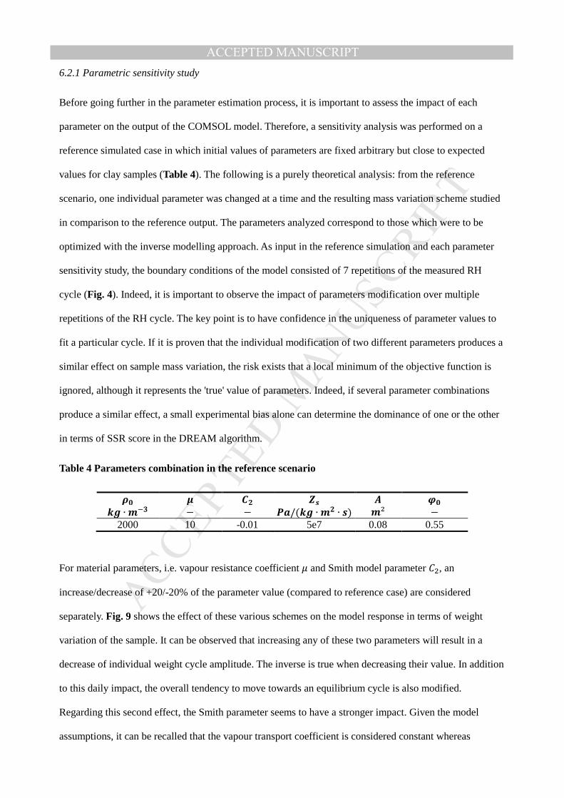
ACCEPTED MANUSCRIPT6.2.1 Parametric sensitivity study
Before going further in the parameter estimation process, it is important to assess the impact of each
parameter on the output of the COMSOL model. Therefore, a sensitivity analysis was performed on a
reference simulated case in which initial values of parameters are fixed arbitrary but close to expected
values for clay samples (Table 4). The following is a purely theoretical analysis: from the reference
scenario, one individual parameter was changed at a time and the resulting mass variation scheme studied
in comparison to the reference output. The parameters analyzed correspond to those which were to be
optimized with the inverse modelling approach. As input in the reference simulation and each parameter
sensitivity study, the boundary conditions of the model consisted of 7 repetitions of the measured RH
cycle (Fig. 4). Indeed, it is important to observe the impact of parameters modification over multiple
repetitions of the RH cycle. The key point is to have confidence in the uniqueness of parameter values to
fit a particular cycle. If it is proven that the individual modification of two different parameters produces a
similar effect on sample mass variation, the risk exists that a local minimum of the objective function is
ignored, although it represents the 'true' value of parameters. Indeed, if several parameter combinations
produce a similar effect, a small experimental bias alone can determine the dominance of one or the other
in terms of SSR score in the DREAM algorithm.
Table 4 Parameters combination in the reference scenario
st u 24 vw x yt !" ∙ &z − − {|/(!" ∙ 4 ∙ w) ² −
2000 10 -0.01 5e7 0.08 0.55
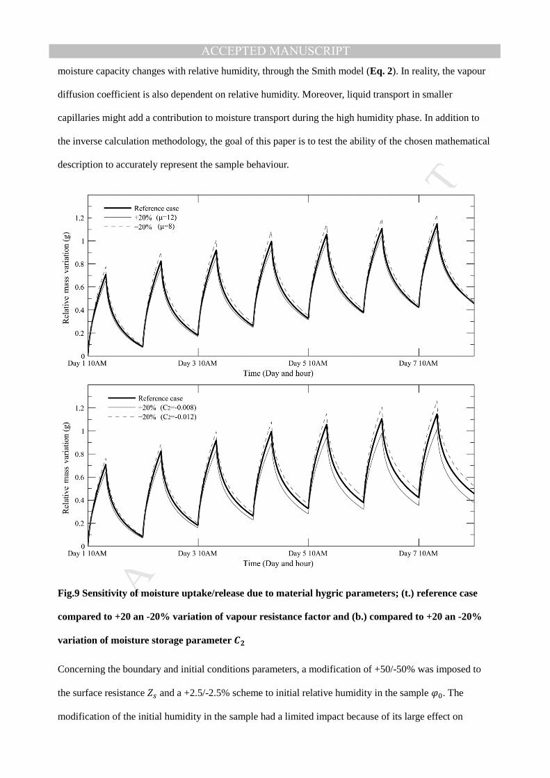
For material parameters, i.e. vapour resistance coefficient $ and Smith model parameter �, an
increase/decrease of +20/-20% of the parameter value (compared to reference case) are considered
separately. Fig. 9 shows the effect of these various schemes on the model response in terms of weight
variation of the sample. It can be observed that increasing any of these two parameters will result in a
decrease of individual weight cycle amplitude. The inverse is true when decreasing their value. In addition
to this daily impact, the overall tendency to move towards an equilibrium cycle is also modified.
Regarding this second effect, the Smith parameter seems to have a stronger impact. Given the model
assumptions, it can be recalled that the vapour transport coefficient is considered constant whereas
MANUSCRIP
T
ACCEPTED
ACCEPTED MANUSCRIPTmoisture capacity changes with relative humidity, through the Smith model (Eq. 2). In reality, the vapour
diffusion coefficient is also dependent on relative humidity. Moreover, liquid transport in smaller
capillaries might add a contribution to moisture transport during the high humidity phase. In addition to
the inverse calculation methodology, the goal of this paper is to test the ability of the chosen mathematical
description to accurately represent the sample behaviour.
Fig.9 Sensitivity of moisture uptake/release due to material hygric parameters; (t.) reference case
compared to +20 an -20% variation of vapour resistance factor and (b.) compared to +20 an -20%
variation of moisture storage parameter 24
Concerning the boundary and initial conditions parameters, a modification of +50/-50% was imposed to
the surface resistance E; and a +2.5/-2.5% scheme to initial relative humidity in the sample (6. The
modification of the initial humidity in the sample had a limited impact because of its large effect on

MANUSCRIP
T
ACCEPTED
ACCEPTED MANUSCRIPTresulting mass variation of the sample. Similarly, surface resistance was modified with +50 and -50% of
its value in order to have a noticeable impact on model output. Fig. 10 presents the simulated relative
weight variation of the reference sample with each of these parameters varied individually, similarly to
Fig. 9. The effect of surface resistance appears to be restricted to daily cycles. The major modification in
comparison to reference cycle occurs at the transition from high to low humidity in the chamber. The
initial RH in the sample has a clear impact on the transition towards equilibrium cycle. It can be explained
easily: if the initial RH corresponds to the average of humidity during the entire day, the cycle would be in
perfect equilibrium from the start. We note that the impact on daily cycle is difficult to assess but is
supposed to be negligible.
Fig.10 Sensitivity of moisture uptake/release due to boundary and initial conditions parameters; (t.)
reference case compared to +50 an -50% variation of surface resistance factor and (b.) compared to

MANUSCRIP
T
ACCEPTED
ACCEPTED MANUSCRIPT+2.5 an -2.5% variation of initial relative humidity in the sample
In order to get a more precise overview about model output sensitivity on parameters modifications,
results of the study can be expressed in terms of sensitivity residuals, defined as:
}� = ~ab�`c, d���e − ab�(c, d′)� (14)
where d��� is the parameter set with reference values (Table 4) and d′ is identical to the reference set with
the modification of one parameter. Fig. 11 shows the sensitivity residuals for all scenarios with increased
values of an individual parameter. Such an approach allows precise identification of the impact on long
term equilibrium and daily cycles of each individual parameter in a highly visual and easily comparable
form. The specific impact of each parameter on the resulting output is clear.
Fig.11 Sensitivity residuals for parameters increase scenarios
The initial relative humidity (6 plays preferentially on long term evolution, with a moderate impact on
daily cycles whereas the exchange surface resistance shows precisely the opposite behaviour. Material
parameters denote a more complex combination of effects. Both impact daily cycles in a similar way but
the � parameter seems able to modify long term evolution in a more noticeable manner. Also, the long
term impact of increasing this moisture storage property appears to be very similar to an increase of initial
humidity in the sample. Given these observations, a combination of +20% on $ value and +1% on (6
value is illustrated to check if the same effect as an increase of � alone can be produced and results are

MANUSCRIP
T
ACCEPTED
ACCEPTED MANUSCRIPTshown on Fig. 12. It seems that producing exactly the same residuals is not possible which gives
confidence for the subsequent optimization task.
Fig.12 Sensitivity residuals for materials parameters
With the results of the sensitivity analysis, we can already draw some conclusions regarding the inverse
modelling approach. First, the model assumptions, and in particular the definition of moisture storage and
transport functions, will determine the ability of the optimization algorithm to extricate a relevant
description of the material. In our case, the inclusion of a RH-dependent moisture capacity potentially
reduces the number of local minima in the ^^ (d'…�) space. It can be assumed that the global best score
in terms of SSR is far from the score of the closest local minima. To take a contradictory example, if
moisture capacity was considered constant in Eq. 5, the DREAM tool would probably have difficulty in
converging towards a single best parameter combination. Of course, the mass variation of a sample during
a MBV experiment does not provide enough information to determine both complex transport and storage
functions. This would probably require the definition of a new non-isothermal cycle in order to create
various vapour pressure and relative humidity gradients in the material.
A second short remark is specific to the use of MBV cycles for parameter evaluation. It appears that the
optimization process should not be performed over one unique mass variation cycle because some
parameter effects only develop over the repetition of RH cycles.
6.2.2 DREAM algorithm outputs
MANUSCRIP
T
ACCEPTED
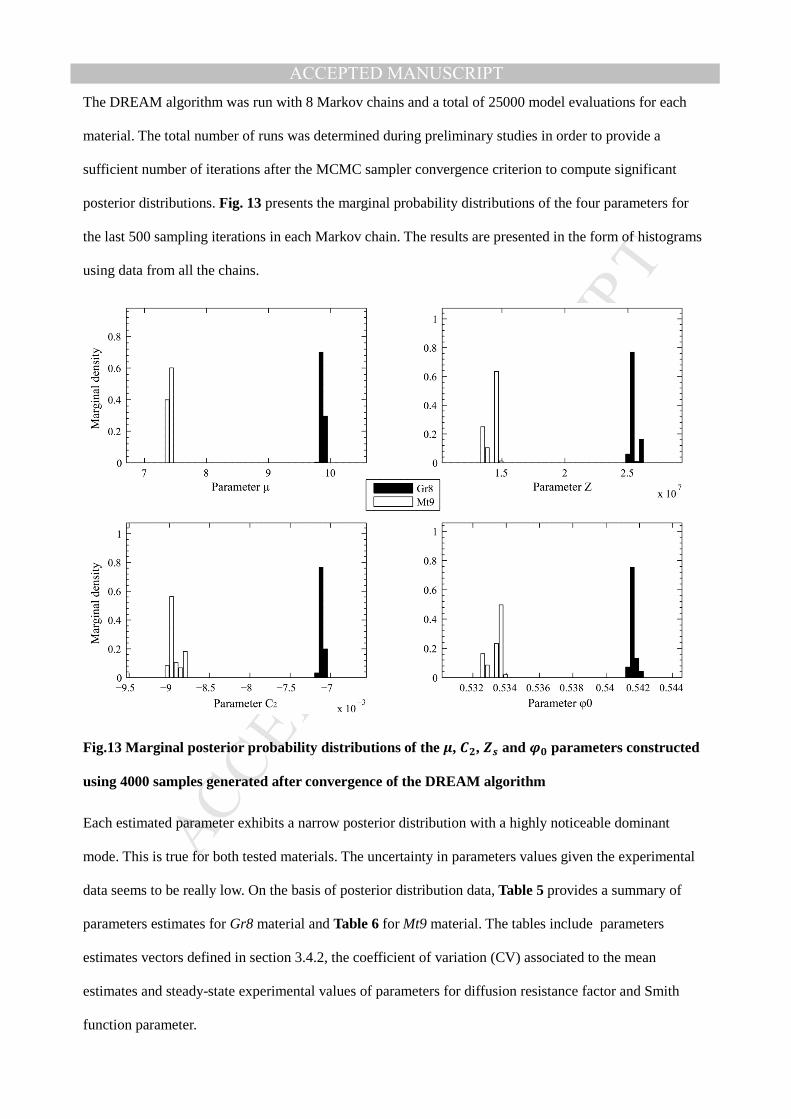
ACCEPTED MANUSCRIPTThe DREAM algorithm was run with 8 Markov chains and a total of 25000 model evaluations for each
material. The total number of runs was determined during preliminary studies in order to provide a
sufficient number of iterations after the MCMC sampler convergence criterion to compute significant
posterior distributions. Fig. 13 presents the marginal probability distributions of the four parameters for
the last 500 sampling iterations in each Markov chain. The results are presented in the form of histograms
using data from all the chains.
Fig.13 Marginal posterior probability distributions of the u, 24, vw and yt parameters constructed
using 4000 samples generated after convergence of the DREAM algorithm
Each estimated parameter exhibits a narrow posterior distribution with a highly noticeable dominant
mode. This is true for both tested materials. The uncertainty in parameters values given the experimental
data seems to be really low. On the basis of posterior distribution data, Table 5 provides a summary of
parameters estimates for Gr8 material and Table 6 for Mt9 material. The tables include parameters
estimates vectors defined in section 3.4.2, the coefficient of variation (CV) associated to the mean
estimates and steady-state experimental values of parameters for diffusion resistance factor and Smith
function parameter.
MANUSCRIP
T
ACCEPTED
ACCEPTED MANUSCRIPT
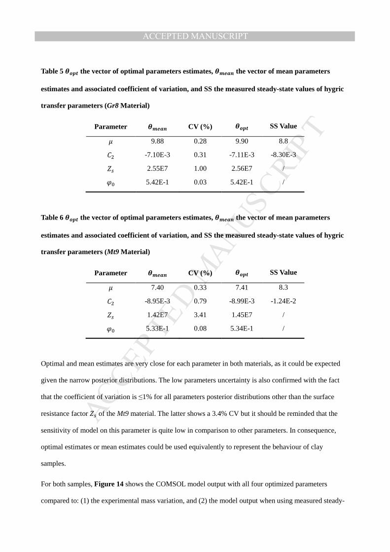
Table 5 ���� the vector of optimal parameters estimates, � �|� the vector of mean parameters
estimates and associated coefficient of variation, and SS the measured steady-state values of hygric
transfer parameters (Gr8 Material)
Parameter � �|� CV (%) ���� SS Value
$ 9.88 0.28 9.90 8.8
� -7.10E-3 0.31 -7.11E-3 -8.30E-3
E; 2.55E7 1.00 2.56E7 /
(6 5.42E-1 0.03 5.42E-1 /
Table 6 ���� the vector of optimal parameters estimates, � �|� the vector of mean parameters
estimates and associated coefficient of variation, and SS the measured steady-state values of hygric
transfer parameters (Mt9 Material)
Parameter � �|� CV (%) ���� SS Value
$ 7.40 0.33 7.41 8.3
� -8.95E-3 0.79 -8.99E-3 -1.24E-2
E; 1.42E7 3.41 1.45E7 /
(6 5.33E-1 0.08 5.34E-1 /
Optimal and mean estimates are very close for each parameter in both materials, as it could be expected
given the narrow posterior distributions. The low parameters uncertainty is also confirmed with the fact
that the coefficient of variation is ≤1% for all parameters posterior distributions other than the surface
resistance factor E; of the Mt9 material. The latter shows a 3.4% CV but it should be reminded that the
sensitivity of model on this parameter is quite low in comparison to other parameters. In consequence,
optimal estimates or mean estimates could be used equivalently to represent the behaviour of clay
samples.
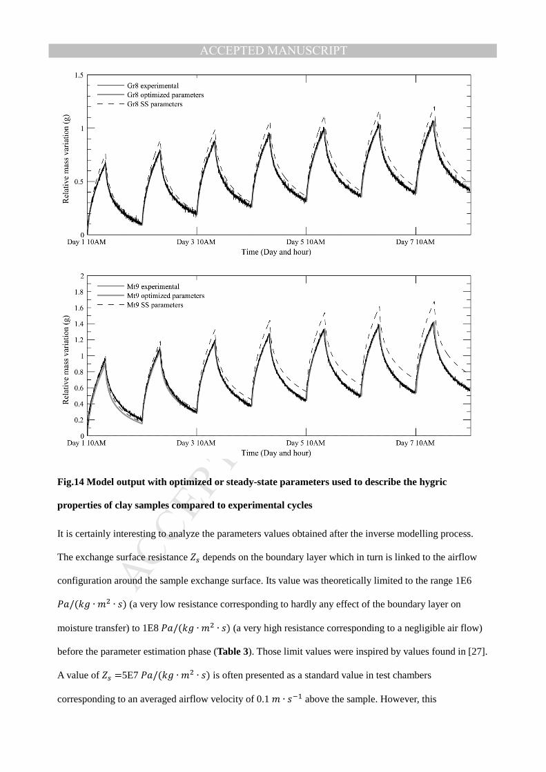
For both samples, Figure 14 shows the COMSOL model output with all four optimized parameters
compared to: (1) the experimental mass variation, and (2) the model output when using measured steady-
MANUSCRIP
T
ACCEPTED
ACCEPTED MANUSCRIPTstate values to describe the vapour permeability and the sorption isotherm of the clay and optimized values
for surface resistance and initial relative humidity in the sample. In consequence, the two model outputs
illustrated only differ in the values of hygric properties for Gr8 and Mt9 samples. The optimal parameter
set results in a ]^K of 0.997 for Gr8 material and a ]^Kof 0.996 for Mt9 material reflecting a very high
efficiency of the model in the description of clay samples mass variation after the optimization process. In
contrast, the measured steady-state properties result in a NSE of 0.875 for Gr8 material and 0.7513 for Mt9
material. The efficiency found for Gr8 sample is very similar to the one found in a previous direct MBV
modelling approach [24] and can already be considered as a good modelling efficiency. Globally, the
optimization process can improve further the fitting to experimental data and potentially reduce the
uncertainty on material and experimental parameters. In particular, when dealing with complex
hygrothermal models, it can be used as a precious tool for reducing the experimental uncertainty linked to
material characterization. As improving the precision in experimental material characterizing can be
expensive and time-consuming, the inverse modelling techniques offers an alternative to consider.
MANUSCRIP
T
ACCEPTED
ACCEPTED MANUSCRIPT
Fig.14 Model output with optimized or steady-state parameters used to describe the hygric
properties of clay samples compared to experimental cycles
It is certainly interesting to analyze the parameters values obtained after the inverse modelling process.
The exchange surface resistance E; depends on the boundary layer which in turn is linked to the airflow
configuration around the sample exchange surface. Its value was theoretically limited to the range 1E6
=>/(�� ∙ ∙ B) (a very low resistance corresponding to hardly any effect of the boundary layer on
moisture transfer) to 1E8 =>/(�� ∙ ∙ B) (a very high resistance corresponding to a negligible air flow)
before the parameter estimation phase (Table 3). Those limit values were inspired by values found in [27].
A value of E; =5E7 =>/(�� ∙ ∙ B) is often presented as a standard value in test chambers
corresponding to an averaged airflow velocity of 0.1 ∙ B&' above the sample. However, this

MANUSCRIP
T
ACCEPTED
ACCEPTED MANUSCRIPTexperimental parameter is often poorly controllable in climate chamber experiments and it seems that
there is still no accurate way to determine it. Inverse modelling estimation can thus provide a solution to
this issue although the quality of the estimation should be confirmed in complementary studies. Here, the
estimated values for surface resistance are close to the reference value but differ between the two
experimental tests. It is difficult to assess the origin of this difference although it can supposedly be caused
by airflow variations from one test to the other, which could result from small difference of sample
location in the chamber. Especially when one knows that the mass variation sensitivity on that parameter
is low around 1E7 =>/(�� ∙ ∙ B) according to [27].
Concerning the initial relative humidity (6 in the material, although its value is supposed to be identical
for both clay samples, the difference is so small it could be imputed to sample manipulation before the
test. The estimated values are close to expected provided the sample conditioning before the test.
The most interesting part in results analysis is of course to discuss the values estimated for the hygric
properties of the materials. Compared to values measured in steady-state, the optimal estimate of vapour
resistance factor $ is 12.5% higher for Gr8 material and 11% lower for Mt9 material. The difference
between the two clay materials is thus more pronounced under the inverse modelling results. Whereas the
steady-state$ parameter is assessed on the basis of a constant mean relative humidity of 72%RH (wet-cup
test), the estimated parameter represents in fact the vapour transport in the active depth of the material,
averaged over various RH conditions met during the 24 hours cycle. Resulting identical values for the two
methods would be particularly astonishing as they not characterize exactly the same behaviour. Still, it is
confirmed that Gr8 material has a higher resistance to vapour transport. For moisture storage parameter
�, characterizing the moisture capacity evolution with relative humidity, the estimated value is
respectively 14% higher for Gr8 material and 28% higher for Mt9 material compared to steady-state
measurement. It corresponds to less moisture storage capacity for both materials (Eq. 3). The higher
moisture storage capacity observed with the DVS method for Mt9 material compared to Gr8 is confirmed
by the inverse modelling approach but less pronounced. Again, the dynamic nature of inverse modelling
estimation must be highlighted. The DVS provides equilibrium sorption isotherms whereas the values
obtained from posterior distributions characterize a dynamic behaviour where equilibrium values are not
perfectly representative. Indeed, a lower moisture capacity for both materials (compared to DVS results)

MANUSCRIP
T
ACCEPTED
ACCEPTED MANUSCRIPTcan mean a kind of 'latency' in moisture sorption.
7. CONCLUSION
An inverse modelling method based on Bayesian techniques and MCMC simulations was tested for
parameter estimation for a moisture transfer model applied to the study of construction materials. The
MBV protocol, dedicated originally to assess the moisture exchange capacity of hygroscopic materials,
was proposed here as an experimental data source from which it is possible to infer information
concerning the moisture storage function and the vapour transport coefficient. But the approach can be
applied theoretically to all kind of HAM models and case studies as long as the HAM model can be
combined numerically to a parameter optimization algorithm.
Two different clay masonry materials were first subjected to repeated 50/85%HR cycles in a 16hrs/8hrs
scheme, similar to the NORDTEST protocol. The monitoring of their weight during this test constitutes
the measurement data intended to be compared with the output of a hygric model. Relevant material
properties involved in moisture uptake/release behaviour were also measured precisely for both samples.
This step included a wet-cup test for vapour permeability determination and a DVS test to assess their
moisture storage at different RH levels.
The numerical model used to describe the moisture transfer in the clay samples during the MBV cycles
was developed in COMSOL and uses a simplified mass balance equation, without liquid transport. Four
parameters were chosen to be optimized in order to fit experimental data. They form two categories: (1)
The materials properties which include the vapour resistance factor and a coefficient characterizing the
evolution of moisture capacity with relative humidity in the porous structure; (2) Experimental parameters
composed of the surface resistance and initial humidity in the sample. A sensitivity analysis showed that
each parameter had a different impact on simulated moisture exchange giving confidence in the
optimization process. The latter was performed with the recently developed DREAM algorithm combined
with the hygric model in the Matlab environment. Compared to other inverse modelling tools, DREAM
offers the advantages of Bayesian techniques and MCMC sampling, i.e. the determination of parameters
posterior distribution with a possible evaluation of the uncertainty of parameters values and model outputs
MANUSCRIP
T
ACCEPTED
ACCEPTED MANUSCRIPTgiven the experimental data.
This study showed that the MBV test provides a relevant ground for the estimation of moisture transfer
properties, in the analysis of highly hygroscopic clay-based material in dynamic conditions. This
experimental protocol provides important information about the material behaviour which can be extracted
with an inverse modelling approach. Inverse modelling is still not very common in Building Physics but
can be very powerful provided the model accurately represents the hygrothermal behaviour. The DREAM
MCMC sampler converged and provided very little dispersed posterior distributions for all parameters. On
this basis, the computed estimates for vapour transport and moisture storage parameters were compared to
their values measured under steady-state conditions. Based on the sensitivity analysis of model output,
there is good confidence in optimized values of parameters and in their representativeness under dynamic
moisture exchange conditions. There is no reason to believe that steady-state parameters provide a 'better'
description of the material behaviour. The differences between steady-state and estimated values could be
partly explained by the dynamic nature of the MBV test which causes complex interactions between
moisture storage and transport phenomena. The estimated parameters through inverse modelling are
potentially more representative of the actual conditions met in a building where steady-state conditions
almost never happen.
Despite these interesting results, the inverse modelling approach requires some precautions as indicated
throughout in the text. First, the experimental acquisition system should be highly reliable as the observed
data uncertainty plays a major role in the optimization process and final parameter estimates. Moreover, a
precise understanding of the model parameters and their effect on model output is required and will help to
determine the ideal number of measurement points to use in the MCMC sampler, in order to maximize
posterior distribution quality and minimize computational time. When appropriate, the model itself has to
be modified through definition of new parameters whose effects on model output can be clearly
distinguished. Nevertheless, if these conditions are respected, the technique is very promising. Numerous
new test protocols could be created to highlight various behaviours of construction materials and continue
the improvement of mathematical models. The inverse modelling approach could also be applied to larger
scale studies where having experimental data for all needed parameters can be tricky or at least a time-
consuming task.

MANUSCRIP
T
ACCEPTED
ACCEPTED MANUSCRIPTREFERENCES
[1] Gandreau D, Delboy L. Inventory of earthen architecture. UNESCO;2012. [2] Minke G. Building with Earth: Design and Technology of a Sustainable Architecture. Basel: Birkhäuser; 2006. [3] Padfield T. The role of absorbent building materials in moderating changes of relative humidity [PhD Thesis]. [Lyngby (DK)]: Technical Univ. of Denmark; 1998. [4] Toftum J, Fanger PO. Air humidity requirements for human comfort. ASHRAE Transactions. 1999;99. [5] Fang L, Clausen G, Fanger PO. Impact of temperature and humidity on the perception of indoor air quality. Indoor Air. 1998;8:80-90. [6] Simonson CJ, Salonvaara M, Ojanen T. The effect of structures on indoor humidity–possibility to improve comfort and perceived air quality. Indoor Air. 2002;12:243-51. [7] Peuhkuri RH, Mortensen LH, Hansen KK, Time B, Gustavsen A, Ojanen T, et al. Moisture Buffering of Building Materials. Lyngby (DK): Technical Univ. of Denmark; 2005 Dec. 78p. Report No: BYG·DTU R-126. [8] Osanyintola OF, Simonson CJ. Moisture buffering capacity of hygroscopic building materials: Experimental facilities and energy impact. Energy and Buildings. 2006;38:1270-82. [9] Künzel HM, Kiessl K. Calculation of heat and moisture transfer in exposed building components. International Journal of Heat and Mass Transfer. 1996;40:159-67. [10] Häupl P, Grunewald J, Fechner H, Stopp H. Coupled heat air and moisture transfer in building structures. International Journal of Heat and Mass Transfer. 1997;40:1633-42. [11] Rode Pedersen C. Combined heat and moisture transfer in building constructions [PhD Thesis]. [Lyngby (DK)]: Technical Univ. of Denmark; 1990. [12] Dos Santos GH, Mendes N. Combined Heat, Air and Moisture (HAM) Transfer Model for Porous Building Materials. Journal of Building Physics. 2009;32:203-20. [13] Hagentoft C-E, Kalagasidis AS, Adl-Zarrabi B, Roels S, Carmeliet J, Hens H, et al. Assessment Method of Numerical Prediction Models for Combined Heat, Air and Moisture Transfer in Building Components: Benchmarks for One-dimensional Cases. Journal of Thermal Envelope and Building Science. 2004;27:327-52. [14] Janssens A, Woloszyn M, Rode C, Sasic-Kalagasidis A, De Paepe M. From EMPD to CFD–overview of different approaches for Heat Air and Moisture modeling in IEA Annex 41. IEA ECBS Annex 41 Closing seminar; 2008 Jun 19; Lyngby, Denmark. [15] Scheffler GA, Plagge R. A whole range hygric material model: Modelling liquid and vapour transport properties in porous media. International Journal of Heat and Mass Transfer. 2010;53:286-96. [16] Dantas L, Orlande H, Cotta R. An inverse problem of parameter estimation for heat and mass transfer in capillary porous media. International Journal of Heat and Mass Transfer. 2003;46:1587-98. [17] Metropolis N, Rosenbluth AW, Rosenbluth MN, Teller AH, Teller E. Equation of state calculations by fast computing machines. The journal of chemical physics. 1953;21:1087. [18] Ter Braak CJ. A Markov Chain Monte Carlo version of the genetic algorithm Differential Evolution: easy Bayesian computing for real parameter spaces. Statistics and Computing. 2006;16:239-49. [19] Vrugt JA, Ter Braak C, Diks C, Robinson BA, Hyman JM, Higdon D. Accelerating Markov chain Monte Carlo simulation by differential evolution with self-adaptive randomized subspace sampling. International Journal of Nonlinear Sciences and Numerical Simulation. 2009;10:273-90. [20] Vrugt JA, Ter Braak CJ, Clark MP, Hyman JM, Robinson BA. Treatment of input uncertainty in hydrologic modeling: Doing hydrology backward with Markov chain Monte Carlo simulation. Water Resources Research. 2008;44. [21] Dumont B, Leemans V, Mansouri M, Bodson B, Destain J-P, Destain M-F. Parameter identification of the STICS crop model, using an accelerated formal MCMC approach. Environmental Modelling & Software. 2014;52:121-35. [22] McGregor F, Heath A, Fodde E, Shea A. Conditions affecting the moisture buffering measurement performed on Compressed Earth Blocks. Building and Environment. 2014. [23] Smith SE. The sorption of water vapor by high polymers. Journal of the American Chemical Society. 1947;69:646-51. [24] Dubois S, Evrard A, Lebeau F. Modeling the hygrothermal behavior of biobased construction materials. Journal of Building Physics. 2013. [25] Chib S, Greenberg E. Understanding the metropolis-hastings algorithm. The American Statistician. 1995;49:327-35. [26] Gelman A, Rubin DB. Inference from iterative simulation using multiple sequences. Statistical science. 1992:457-72. [27] Roels, S, Janssen, H. Is the moisture buffer value a reliable material property to characterize the hygric buffering capacities of building materials. Working paper A41-T2-B-05-7 for IEA Annex 41 project. 2005