analysis of packet loss probing in packet...
TRANSCRIPT

1
Analysis of Packet Loss Probing
in Packet Networks
By
Maheen Hasib
SUBMITTED FOR THE DEGREE OF DOCTOR OF
PHILOSOPHY
Supervised by Dr. John Schormans
Department of Electronic Engineering
Queen Mary, University of London
June 2006

2
To my parents

3
Authorship Declaration
This is to certify that
i. the work presented in this thesis is the author’s own.
ii. due acknowledgement has been made in the text to all other material
used
iii. the thesis is less than 100,000 words in length (including footnotes),
exclusive of tables, maps, bibliographies and appendices.
Maheen Hasib
Department of Electronic Engineering
Queen Mary, University of London
June 2006
4
Abstract
Performance measurement of managed IP packet networks is focused on
monitoring network performance, including availability, packet loss and
packet delay statistics. Performance monitoring is a vital element in the
commercial future of broadband packet networking and the ability to
guarantee quality of service in such networks is implicit in Service Level
Agreements. Network performance can involve many different aspects, but
this thesis focuses on what are often called the quality of service metrics:
packet loss and delay, and most specifically loss. Network operators and
service providers should be aiming to keep within the limits prescribed by
standards for both delays (in particular the mean delay) and packet loss
ratio.
A number of technological approaches have been proposed for packet level
measurement and monitoring, but all are essentially schemes based on
sampling. Furthermore, the growing need to operate over global-scale
networks means that sampling techniques based on packet probing are
likely to be of increasing significance in the near future. These probing
techniques all rely on inferring the loss and delay statistics seen by users
from a necessarily limited number of samples of the network performance.

5
The main contribution of this thesis is the development of an analytical
technique, based on the variance of the inter-packet loss distribution, which
provides an accurate assessment of how many samples will be required to
accurately estimate packet loss probabilities via sampling. From the key
observation, based on extensive prior work, that the stochastic process
representing the queue backlog in packet buffers is a highly bursty process,
this thesis develops analytical techniques to bound the performance of any
packet level sampling scheme. The analysis has been tried under various
traffic scenarios, including well accepted Markovian and Power-law traffic
models, and has been validated by comparison with simulations.
It is anticipated that the findings of this thesis has the potential to be of great
value to network operators and service providers.

6
Acknowledgements I would like to first thank God for giving me the strength to complete this
thesis. I am deeply indebted to my supervisor, Dr. John Schormans whose
help, stimulating suggestions and encouragement helped me during my
research and writing of this thesis. John, thank you ever so much for your
constant support, advice, constructive comments and guidance without
which it would not have been possible to complete this thesis.
I would like to thank everybody in the Department of Electronic
Engineering at Queen Mary, University of London for creating such a
friendly working environment. My special thanks go to Prof. Laurie
Cuthbert, Prof Jonathan Pitts, Dr. Chris Phillips, Dr. Raul Mondragon, Sue
Taylor, Lynda Rolfe, Kay Parmer, Michele Pringle, Theresa Willis, Phil
Wilson and Kok Ho Huen. I would also like to thank my ns2 buddies ☺
Vindya, Rupert and Touseef. Long Live “Room 402”. I will miss all the nice
chats we had.
I would like to thank my four pillars of strength my parents, Jolly-
Maa and my brother Ishaque for their constant love and prayers.
Finally, I would like to show my deepest gratitude towards Sharifah
and Ali for their constant encouragement and help towards building my
confidence. I would like to thank them for always motivating me and
providing me with their endless friendship, love and support.

7
Table of Contents Authorship Declaration ........................................................................................... 3
Abstract ...................................................................................................................... 4
Acknowledgements ................................................................................................. 6
Table of Contents...................................................................................................... 7
List of Figures.......................................................................................................... 10
List of Tables ........................................................................................................... 12
Glossary ................................................................................................................... 13
List of Mathematical Symbols .............................................................................. 16
1 Introduction..................................................................................................... 18
1.1 Research Motivation ...............................................................................18 1.2 Aim and Objective of the Thesis ...........................................................24 1.3 Novelty and Contribution towards the Research...............................25 1.4 Thesis Layout ...........................................................................................25
2 Network Measurement of Packet Networks.............................................. 29
2.1 Why Network Measurement? ...............................................................29 2.1.1 Service Level Agreements..............................................................31
2.2 Network Management ............................................................................34 2.2.1 Simple Network Management Protocol.......................................36 2.2.2 Management Information Base.....................................................37
2.3 Network Measurement Techniques .....................................................38 2.3.1 Passive Measurements....................................................................39
2.3.1.1 Hardware-based Passive Measurement...................................40 2.3.1.2 Software-based Passive Measurement (Tcpdump) ................41 2.3.1.3 Polling MIB...................................................................................42
2.3.2 Active Measurement.......................................................................43 2.3.2.1 PING..............................................................................................45 2.3.2.2 Traceroute.....................................................................................48 2.3.2.3 One-Way Active Measurement Protocol .................................49
2.4 Organizations Standardising Network Measurements.....................50 2.4.1 Internet Engineering Task Force (IETF) .......................................51

8
2.4.2 Cooperative Association for Internet Data Analysis (CAIDA) 54 2.4.3 National Laboratory for Applied Network Research (NLANR) 56
2.5 Applications of Network Measurements.............................................59 2.5.1 Network Tomography....................................................................60 2.5.2 Measurement-based Admission Control .....................................61 2.5.3 Available Bandwidth Estimation..................................................62
2.6 Summary ..................................................................................................65 3 End-to-End Packet Loss Issues..................................................................... 67
3.1 Why is Loss Important?..........................................................................67 3.1.1 UDP and TCP based applications.................................................67
3.2 Causes of Packet Loss .............................................................................70 3.3 Traffic Models ..........................................................................................71
3.3.1 Short-Range Dependent Traffic Models ......................................72 3.3.2 Long-Range Dependent Traffic Models.......................................75
3.4 Why On/Off Models? .............................................................................75 3.5 Queueing Behaviour for a FIFO Buffer Multiplexing Markovian Traffic 77 3.6 Summary ..................................................................................................78
4 Overflow Analysis for Single Buffered Links ............................................ 80
4.1 The Loss Model for a Buffered Link.....................................................80 4.2 Loss Cycle Time Analysis ......................................................................82 4.3 Analysing the interaction between the probe stream and the buffer overflows..............................................................................................................87 4.4 The Loss Model for an End-to-End Network......................................91 4.5 Loss Cycle Time Analysis for n queues in series................................93 4.6 Numerical Examples using the analysis..............................................94 4.7 Summary ..................................................................................................98
5 Sampling Theoretic Bounds on the Accuracy of Probing ........................ 99
5.1 Variability of the distribution of the number of packets between lost packets for a buffered link .................................................................................99 5.2 Measuring an end-to-end path across a realistic network ..............108 5.3 Numerical Examples.............................................................................111
5.3.1 Measurement (Simulation) Time ................................................111 5.3.2 Results.............................................................................................112 5.3.3 Effect on the Probes and on the Number of Busy Hours Required for Sampling .................................................................................117
5.4 Summary ................................................................................................122 6 Measuring Power Law Traffic using Active Probing ............................. 124

9
6.1 Self-Similarity and Long Range Dependence...................................124 6.2 Simulation Model ..................................................................................129
6.2.1 Verification of ExPareto traffic source (using Geo/Pareto/1)130 6.2.2 Parameters used for the Simulation ...........................................133
6.3 Buffer Length Analysis and its Limitations.......................................134 6.4 Simulation Results.................................................................................138 6.5 Effect on the probes and on the number of busy hours required for sampling.............................................................................................................140 6.6 Effect of the shape parameter on the number of samples ...............140 6.7 An Issue of Measurement (Simulation) Time ...................................144
7 Conclusion and Future Work ..................................................................... 146
7.1 Conclusion ..............................................................................................146 7.2 Future Work...........................................................................................152
8 Appendices.................................................................................................... 155
Appendix A: Queue Length Distribution for Markovian Traffic ...............155 Packet-Scale Queueing .................................................................................155 Burst-Scale Queueing....................................................................................156
Appendix B: Comparison of T(ON) with Expected Overflow Duration E(OF) ..................................................................................................159 Appendix C: Calculation of the steady state probability, s(k)....................160 Appendix D: Design Rules for Buffering Overlapping Pareto Sources ................................................................................................................163
9 Author’s Publications.................................................................................. 167
10 References .................................................................................................. 168
10
List of Figures Figure 2-1 Network Measurement Metrics [51] ................................................. 31 Figure 2-2 Network management functional grouping [62] ............................ 35 Figure 2-3 SNMP Network Model ....................................................................... 37 Figure 2-4 Passive Measurement (packet sniffing) ............................................ 40 Figure 2-5 One-way and Two-way Active Measurement ................................ 44 Figure 2-6 ICMP PING implementation............................................................. 46 Figure 2-7 A PING example.................................................................................. 47 Figure 2-8 A Traceroute example ......................................................................... 48 Figure 2-9 IPPM One Way Active Measurement .............................................. 49 Figure 2-10 The PGM for estimating available bandwidth [108] .................... 64 Figure 3-1 IPP model.............................................................................................. 73 Figure 3-2 Superposition of N voice sources...................................................... 73 Figure 3-3 ON/OFF model .................................................................................. 74 Figure 3-4 Queueing Behaviour for a FIFO multiplexing Markovian Traffic 77 Figure 4-1 Loss Model ........................................................................................... 81 Figure 4-2 State space reduction method [44] .................................................... 83 Figure 4-3 Sojourn time in aggregate ON state .................................................. 85 Figure 4-4 Lower bound for the mean cycle time.............................................. 87 Figure 4-5 Effect on the probe stream.................................................................. 88 Figure 4-6 Schematic representation ................................................................... 88 Figure 4-7 End-to-end network model ................................................................ 93 Figure 4-8 Time for the probes to encounter an overflowing buffer.............. 97 Figure 4-9 Effect of different probe rates ............................................................ 97 Figure 5-1 Schematic Representation of the overflow / non-overflow periods
......................................................................................................................... 101 Figure 5-2 Schematic representation of “q” ...................................................... 103 Figure 5-3 A generic model for an end-to-end network scenario ................. 109 Figure 5-4 Simplified topology for a “generic” network................................ 110 Figure 5-5 PLP plot over simulation time ......................................................... 112 Figure 5-6 Schematic representation of the overflow periods for a load of
65%.................................................................................................................. 115 Figure 5-7 Schematic representation of the overflow periods for a load of
85%.................................................................................................................. 115 Figure 5-8 Comparing the number of samples required single buffer and
end-to-end network ..................................................................................... 116 Figure 5-9 Number of busy hours required by probes for PLP of 10-4 ......... 121 Figure 5-10 BT MPLS Weekly Customer Network Performance Summary
Report ............................................................................................................. 122 Figure 6-1 Comparison of Exponential and Pareto Distributions ................. 127 Figure 6-2 Comparison of Exponential and Pareto Distributions, with
Logarithmic Scale for x ................................................................................ 128

11
Figure 6-3 Comparison of Exponential and Power-law On times ................ 129 Figure 6-4 ExPareto On/Off Model................................................................... 130 Figure 6-5 Model of Arriving Batches of Packets ............................................ 131 Figure 6-6 Verification of ExPareto Source....................................................... 133 Figure 6-7 Relationship between the load and the buffer length using
Equation 6-3 .................................................................................................. 135 Figure 6-8 Comparison of Simulation with Equation 6-9............................... 136 Figure 6-9 PLP with varied loads and buffer length ....................................... 138 Figure 6-10 Calculation of the number of samples.......................................... 139 Figure 6-11 Number of busy hours required by the probes to achieve a PLP
of 10-4 .............................................................................................................. 140 Figure 6-12 Effect of different shape parameters on the PLP for a load of 0.1
......................................................................................................................... 141 Figure 6-13 Effect of different shape parameters on the PLP for a load of 0.2
......................................................................................................................... 142 Figure 6-14 Number of samples required for load of 0.1 .............................. 143 Figure 6-15 Number of samples required for load of 0.2 .............................. 144 Figure 6-16 Running sample mean for exponential distribution with rate
1/60 [172] ....................................................................................................... 145 Figure 6-17 Running sample mean for Pareto distribution with a=1.2 and
k=10 [172]....................................................................................................... 145 Figure 7-1 Queue State Probability for Load = 69.5%..................................... 147 Figure 7-2 Queue State Probability for Load = 79.9%..................................... 148 Figure 7-3 Queue State Probability for Load = 84.5%..................................... 148 Figure 7-4 Queue State Probability for Load = 87.9%..................................... 148 Figure 7-5 diagrammatic representation of the minimising effect on traffic
burstiness of higher bandwidth ................................................................. 151 Figure C-8-1 How to reach state 0 at the end of a time slot ........................... 160 Figure C-8-2 How to reach state 1 at the end of a time slot ........................... 161

12
List of Tables Table 2-1 An example of QoS parameters per class of service defined in a
SLA (quoted from Quasimodo Project: http://www.eurescom.de/public/projects/P900-series/P906/default.asp)............................................................................... 33
Table 3-1 Classes of Service (CoS) [48] ................................................................ 70 Table 4-1 Calculation of the buffer length for single access and end-to-end
networks .......................................................................................................... 96 Table 5-1 Calculation of the number of not lost packets between losses ..... 100 Table 5-2 Comparing variance for a single buffer by simulation and analysis
......................................................................................................................... 113 Table 5-3 Comparing variance for an end-to-end network by simulation and
analysis........................................................................................................... 114 Table 5-4 Number of busy hours required by the probes for a PLP of 10-4 . 117 Table 5-5 Number of busy hours required by the probes for a PLP of 10-4 . 118 Table 5-6 Number of busy hours required by the probes for a PLP of 10-4 . 118 Table 5-7 Number of busy hours required by the probes for a PLP of 10-3 . 119 Table 5-8 Number of busy hours required by the probes for a PLP of 10-3 . 120 Table 5-9 Number of busy hours required by the probes for a PLP of 10-3 . 120 Table 6-1 Calculation of the buffer length ........................................................ 135 Table 6-2 Calculation of the buffer length from simulation for a load of 10%
......................................................................................................................... 136 Table 6-3 Calculation of the buffer length from simulation for a load of 20%
......................................................................................................................... 137 Table 6-4 Calculation of the buffer length from simulation for a load of 30%
......................................................................................................................... 137 Table 6-5 Calculation of the buffer length from simulation for a load of 59.2%
......................................................................................................................... 137 Table 6-6 Calculation of the buffer length from simulation for a load of 67.6%
......................................................................................................................... 137 Table 6-7 Calculation of the buffer length from simulation for a load of 78.7%
......................................................................................................................... 137 Table 6-8 Calculation of the buffer length from simulation for a load of 94.1%
......................................................................................................................... 138 Table 6-9 Calculation of the variance by simulation....................................... 138

13
Glossary AMP Active Management Project
AMT Active Monitoring Tools
ASN Abstract Syntax Notation
ATM Asynchronous Transfer Mode
CAC Connection Admission Control
CAIDA Cooperative Association for Internet Data Analysis
CMIP Common Management Internet Protocol
CoS Class of Service
CPN Corporate Premises Network
DAST Distributed Applications Support Team
DiffServ Differentiated Services
DNS Domain Name System
FIFO First In First Out
FTP File Transfer Protocol
2.5G 2.5 Generation
3G 3 Generation
HPC High Performance Connection
ICMP Internet Control Message Protocol
IETF Internet Engineering Task Force
IGMP Internet Group Management Protocol

14
IP Internet Protocol
IPPM Internet Protocol Performance Metrics
ISO International Organization for Standardization
ITU-T Internet Telecommunication Unit - Telecommunication
LAN Local Area Network
LRD Long Range Dependent
MBAC Measurement Based Admission Control
MIB Management Information Base
MMPP Markov Modulated Poisson Process
MNA Measurement and Network Analysis
MPLS Multi Protocol Label Switching
MTBF Mean Time Between Failure
MTTR Mean Time To Repair
NAI Network Analysis Infrastructure
NLANR Network Laboratory for applied Network Research
NOC Network Operations Centre
NP Network Performance
NS Network Simulator
NSF National Science Foundation
NSP Network Service Provider
OWAMP One Way Active Measurement Protocol

15
PLP Packet Loss Probability
PMA Passive Measurement and Analysis
QoS Quality of Service
RED Random Early Discard
RFC Requests for Comments
RMON Remote Monitoring
RTD Round Trip Delay
RTT Round Trip Time
SAA Service Assurance Agent
SLA Service Level Agreement
SNMP Simple Network Management Protocol
SRD Short Range Dependent
TMN Telecommunication Management Network
TTL Time To Live
TWAMP Two Way Active Measurement Protocol
UDP User Datagram Protocol
VoIP Voice over Internet Protocol
VPN Virtual Private Network
WG Working Group
WRED Weighted Random Early Discard

16
List of Mathematical Symbols C Output capacity of the buffer (link capacity)
Ton Mean ON time (seconds) for an individual ON/OFF source
Toff Mean OFF time (seconds) for an individual ON/OFF
source
h ON rate of an individual ON/OFF source
Ron Mean rate in the ON state
Roff Mean rate in the OFF state
Ap Mean packet arrival rate to the buffer in packets per second
No Maximum number of packet flows that can be served
simultaneously
T(ON) Mean time the aggregate process spends in the ON state
T(OFF) Mean time the aggregate process spends in the OFF state
E(OF) Mean duration of buffer overflow period
µp Expected number of packets lost per overflow period
Tcycle Mean duration of a cycle’s overflow and non-overflow
period
µt Mean time until a probe encounters an overflow (in hours)
Np/cycle Mean number of packets in one cycle
Pr{pof} Probability of the probes hitting an overflow period
Tp Time between probes
P(miss) Probability of the probes missing an overflow period
?m Mean of the Geometric distribution for the number of
probes missing an overflow period
IPLP Individual Packet Loss Probability
TPLP Total Packet Loss Probability
n Number of end-to-end buffers
E[Y] Mean number of not-lost packets between lost packets (=
PLP-1)

17
NOF Mean number of not-lost packets between consecutive lost packets during overflow periods
NNOF Mean number of packets in non-overflow periods
q Prob(an inter-packet-loss period is contained within
overflow period)
1/p Mean of the Geometric distribution
2
1p
p− Variance of the Geometric Distribution
2
2
2
211p
ppp
p −=
+−
Mean square for the Geometric Distribution
EOF[Y2] Mean square number of packets between lost packets given we are considering the first 1−pµ out of pµ lost packets
ENOF[Y2] Mean square number of packets between lost packets given
we are considering the last one of the pµ lost packets Var(Y) Total variance of the distribution of the number of not-lost
packets between lost packets N Number of measurements required
tN-1, 1-α/2 Student t-distribution value for N-1 degrees of freedom
δ Chosen value of absolute error in the measurements
SN Standard deviation of the distribution
S2N Variance of the distribution
? Load

18
1 Introduction
1.1 Research Motivation Until recently, Internet Protocol (IP) networks supported only a best effort
service, which worked very well with conventional Internet applications like
file transfer, Electronic mail (email) and Web Browsing, because of their
ability to cope with packet losses and varying packet delays [1][2][3].
However, best effort does not satisfy the needs of many new applications
like audio and video streaming, which demand high data throughput
(bandwidth) and have low-latency requirements [1][4][5]. Thus, managed IP
networks are coming to dominate the way information is brought to users on
a worldwide basis and is typically accomplished by isolating the routers,
links etc used to provide the IP service to a particular user and using these
resources for that user alone. In some cases, the routers and links are still
shared, but only among the users that have contracted for managed IP
services [6]. That is why Differentiated Services (DiffServ) and Multi
Protocol Label Switching (MPLS) are emerging technologies, which are
being used to provide the managed IP services in many organisations like
Global Crossing, Cisco, MCI, British Telecoms, Lucent technologies and
Juniper networks [7] [8] [9] [10] [11] [12]. For example, Global Crossing has a
versatile and fully managed IP Virtual Private Network (VPN) solution [7],
which provides end-to-end managed services environment where data,

19
voice, video and multimedia applications are supported on a single IP-based
platform. It is clear that the commercial importance of managed IP
networking solutions is set to grow over time. In conjunction with this, the
number of users and the range and heterogeneity of applications has both
increased, and therefore so has the demand for guaranteed Quality of
Service (QoS) [13]. Network Performance (NP) means loss and delay, and
the ability of networks to guarantee and maintain certain performance levels
for each application according to the specified needs of each user, critically
affects what the user sees as “QoS”. In response to this, Network and Service
Providers (NSPs) are aiming to provide Service Level Agreements (SLAs)
[14] [15]: a service contract between a NSP and a subscriber that aims to
quantify the strictly user experience by tightly bounding the NP (typically
mean delay, delay jitter and packet loss probability (PLP)) that will be
guaranteed to each class of traffic and therefore, each user/application
within that class.
Network performance measurement is the key to the provision and
maintenance of such agreements. The two main approaches that are used to
measure the QoS performance are called Passive and Active monitoring [16]
[17] [18] [19] [20]. The former non-intrusively monitors the traffic by using
access to the routers directly, where available, while the latter injects probes
(empty packets) into the network and therefore can be used across network

20
boundaries. It also provides global reach to support globally significant new
services at 3G and beyond.
Passive monitoring is a means of tracking the performance and behaviour of
packet streams by measuring the user traffic without creating new traffic or
modifying existing traffic. It is implemented by incorporating additional
intelligence into network devices to enable them to identify and record the
characteristics and quantity of the packets that flow through them. The level
of detail provided by the performance statistics is dependent on the network
metrics of interest, how the metrics are processed, and the volume of traffic
passing through the monitored devices. Examples of the types of
information that can be obtained using passive monitoring are [17] [21] [22]:
• Bit or packet rates
• Packet timing / inter-arrival timing
• Queue levels in buffers (which can be used as indicators of packet loss
and delay)
• Traffic / protocol mixes
Recently published work has shown that passive monitoring can be
extremely accurate [21] [23] [24] [25] [26] [27]. Unfortunately the cost of
using this method can be high due to increasing data-storage requirements,
and a critically limiting consideration is that access across administrative

21
domains may not be possible [18]. The main drawback of passive monitoring
is that it requires full access to network resources (e.g. routers, perhaps via
Simple Network Management Protocol (SNMP) ) otherwise it is impossible
to combine into an end-to-end QoS over a number of separately owned and
operated networks. This drawback is likely to be very common in an era of
growing globalisation of business opportunities: access to all the relevant
equipment's internal measurements is not possible. With the increasing
number of organisations like Global Crossing and British Telecom, wanting
to give customers global access, Active Probing is becoming the default
means of network measurement [19], and a considerable amount of recent
work has concentrated on developing these techniques [28] [29] [30] [31] [32]
[33].
Active monitoring works by injecting extra test packets (probes) into the
network, irrespective of the details of the probing technology itself. The best
known example is the Cisco IOS Service Assurance Agent (SAA) [34].
Cooperative Association for Internet Data Analysis (Caida) and National
Laboratory for Applied Network Research (NLANR) [33] [35] [36] report the
use of active probing to measure network health, perform network
assessment, assist with network troubleshooting and plan network
infrastructure.

22
There are many variations of the basic probing scheme: single packet probes,
packets pairs, triples etc, and variations in the pattern of probe delivery -
Poisson probing, deterministic etc [37].
Measurement of the PLP is likely to be more challenging than measuring
mean packet delay, as it naturally involves quantifying tail probabilities,
rather than just average values. Furthermore, measuring the packet loss
episodes caused by buffer overflows is complicated by overflow events
being randomly distributed over time and have rare occurrence [19] [32] (it
is not the intention in this thesis to study the effect on measurements of
packet losses due to link failures) hence making it more difficult to measure.
[38] measured the Round trip time (RTT) delays of User Datagram Protocol
(UDP) probe packets sent at regular time intervals to analyse the end-to-end
loss behaviour in the Internet. [38] has also shown that the loss probability
increases when the inter-probe arrival becomes very small because the
contribution of the probe packets to the buffer queue length was non-
negligible. In [39] queueing analysis has been used to show that, for a tail-
drop queue, probes would need to be of very similar length to the packet
traffic whose loss probability is being measured, else the measured loss
probabilities could easily be in error by many orders of magnitude.
Therefore, if probes are small packets, they will not necessarily be lost when

23
the large packets are and hence small probe packets cannot accurately be
used to measure the PLP for larger packets.
Some research has been published that aims to bound the accuracy
achievable when probing mean delay and loss [40] [41] [42] . The general
conclusion of these papers is that measurement accuracy obtained, when
probing, may be prone to considerable error. However, while probe tools are
commonly reported as being widely used to measure packet loss, there has
been very little published work on analysis of the accuracy of these tools and
the limitations of probing in packet networks. This motivates this research
work to study the limitation of active probing for PLP measurement. In this
thesis, an analytical approach is developed to show that probing for PLP is
limited by the mean time until a probe is lost, which can be very long (in
hours). Hence it is imperative that NSPs are aware of the time required for
data collection when monitoring the SLAs for different loads.
It is known from sampling theory that the greater the variability of the
sampled data the more samples are needed for accurate estimation [41] [43].
In the case of actively probing packet networks the variability is dependent
on two main factors: the load on the network, and the type of traffic being
carried. Highly bursty packet network traffic results in very large variances
associated with the queue backlog. This is critically important, as using

24
packet networks to carry bursty traffic implies that a very large number of
probes may be needed to achieve the required levels of accuracy [39].
Research to date [37] [16] [39] [40] [41] [43] has used sampling theory to
show that a perfect probing scheme will not necessarily evaluate even just
the mean delay to the required degree of accuracy. The burstier the traffic,
the more variable the queueing/delay distributions and hence more probes
needed to accurately estimate the mean delay. This further motivates this
research work to develop an enhanced form of the previous analysis which
calculated the variance of the number of not-lost packets between packet
losses. This allowed the predictions of the number of samples, and hence
time required, to accurately measure the PLP across a networked path
within predefined measurement error.
1.2 Aim and Objective of the Thesis The overall aim is to investigate the accuracy of probing for PLP.
The objectives of this research are:
• To develop an analytical approach to show that probing for PLP is
limited by the mean time until a probe is lost, which can be very long
(in hours).
• To further develop an enhanced analytical approach for Markovian
traffic to calculate the variance of the inter-packet loss distribution,

25
and thereby find the number of samples needed for a desired level of
accuracy.
• To validate analysis against simulations.
• To extend the study to include power law model e.g. for data traffic.
1.3 Novelty and Contribution towards the Research
In this research work, a novel analytical approach was developed to bound
the accuracy of packet loss probing. This analysis provides a method for:
• Finding the mean time required by the probes to encounter the first
overflow period. This work has been published in Electronic Letters
[19].
• Finding the number of samples required to measure a PLP with the
required degree of accuracy. This is very significant for NSP, as they
need these results for appropriate data collection for SLA monitoring
as discussed in chapter 5. This work has been submitted to the IEE
Communications Proceedings.
1.4 Thesis Layout This thesis comprises of four parts: background of the research, proposed
method, evaluation and applications. It is organised as follows:

26
Chapter 2 revisits the motivation for network measurement in more detail.
Network measurement is an essential process found in the normal network
operations. Network management and its tools: SNMP and Management
Information Base, MIB are reviewed. The two basic measurement schemes:
Active and Passive Measurement and their variants found in the industry
are studied and the features, merits and the shortcomings of these two
schemes are discussed. This chapter also discusses the three organizations
involved in Network Measurements: Internet Engineering Task Force (IETF),
NLANR and CAIDA. Finally, the applications of Network Measurements
are reviewed.
Chapter 3 discusses end-to-end packet loss issues. The two causes of packet
losses, link failures and buffer overflows, are also discussed. The two major
classes of traffic model: Short-Range Dependent SRD traffic and Long-Range
Dependent LRD traffic are reviewed. SRD traffic (e.g. Markovian traffic) has
been long used to model voice traffic. However, recent publications show
that the Markovian traffic model fail to represent data traffic, which may
have Long-Range Dependent properties. This chapter also highlights the
choice of model used in this research: the On/Off model.

27
Chapter 4 develops the analytical approach for evaluating the mean time for
the probes to encounter an overflowing buffer, concentrating on access links
and Markovian traffic.
Chapter 5 presents an enhanced form of the analysis which calculates the
variance of the inter-packet loss distribution (which itself accounts for the
inherent burstiness of the buffer overflow process, and hence the packet loss
events) of the Markovian traffic. The analysis works by capturing the
variance of the number of not-lost packets between losses, and then using it
to estimate the number of samples (probes) required to accurately measure
the PLP across a networked path, within a predefined measurement error.
The analysis is validated by comparison with simulation studies.
Chapter 6 measures the variance of the number of not-lost packets between
losses for self-similar traffic models. Self-similar traffic is vastly different
from traditional voice and data traffic models, and this chapter discusses the
variability of such traffic and the extremely long packet-trains that are
encountered. It shows that the measurability of the packet loss probability
worsens when the network traffic becomes burstier, as it will do when the
data traffic is driven by Power law distributions.

28
Chapter 7 consists of discussions and summary of the research work. In
addition, future work related to this research is addressed.

29
2 Network Measurement of Packet Networks This chapter discusses the motivation of packet network measurement in
detail.
2.1 Why Network Measurement? Network measurement becomes an essential tool to collect information for
the following purposes:
• Network performance evaluation – e.g. throughput, QoS performance
metrics, testing of new technologies and applications.
• Study network properties – e.g. traffic, path, link characteristics.
• Report generation – Service Level Agreement (SLA) validation [34].
• Assisting the network operations – e.g. dimensioning, capacity
planning, network monitoring and fault identification [44].
• Input for decision-making schemes – e.g. MPLS traffic engineering,
routing, Connection Admission Control (CAC).
The need for measurement of performance parameters to support
operations, management and planning of networks has increased in recent
years. One reason is that managed IP networks are coming to dominate the
way information is brought to users on a worldwide basis. They are no
longer limited to transferring data but are also the carrier for multi service

30
communications, and many of the new applications demand high data
throughput (bandwidth) with strict performance requirements [1] [4] [5]
[45]. Hence, without measurements, there will be no objective record or
benchmark of how a network behaves. Measurements show whether
changes improve or degrade the network’s performance, and by how much
[46]. When service performance degradation occurs, these are the common
questions asked by the network administrator or user [47]:
• Why is the application so slow?
• Why there is loss of data?
• What can be done to improve performance?
• Will additional bandwidth help?
Information must be collected by measurements in order to provide answers
to these questions. For example, measurement for capacity planning
provides the information for network operators to calculate necessary
capacity, in order to avoid congestion in the network. The degradation of
performance may cause long packet delay time, jitter or larger packet loss
ratio. For Voice over IP (VoIP), the voice quality is not acceptable if the
packet loss probability is less than 10-3 [48] [49] [50] otherwise it becomes
subject to audible interference, e.g. in the form of clicks. Network
measurement is necessary to monitor the network performance and to
analyse and identify any faults.

31
Figure 2-1 Network Measurement Metrics [51]
Figure 2-1 depicts the common network measurement metrics. These factors
are availability, packet loss, delay and throughput. Network measurement
may be performed in order to assess all of them. With reference Figure 2-1,
the loss metrics can be end-to-end (one-way) loss and round trip loss.
2.1.1 Service Level Agreements
SLAs constitute a service contract between a service provider and a
subscriber that aims to quantify the strictly user experience by tightly
bounding the Network Performance (typically mean delay, delay jitter and
PLP) that will be guaranteed to each class of traffic. Network performance
measurement is the key to the provision and maintenance of such

32
agreements. An SLA typically contains the following information [15] [52]
[53] [54]:
• A description of the nature of the service to be provided.
• The expected performance level of the service, specifically its
reliability and responsiveness.
• The procedure for reporting problems with the service.
• The time frame for response and problem resolution.
• The process for monitoring and reporting the service level.
• The consequences for the service provider not meeting its obligations.
• Escape clauses and constraints.
The following are the performance metrics that are commonly specified in a
SLA [55]:
• Availability – the likelihood of the service is available to the customer
• MTTR – (Mean time to repair) the average time required to fix the
problem or failure
• MTBF – (Mean time between failure) the average time between two
consecutive failures to happen.
• QoS parameters – Latency, Jitter, Loss.

33
Table 2-1 An example of QoS parameters per class of service defined in a SLA (quoted from Quasimodo Project: http://www.eurescom.de/public/projects/P900-
series/P906/default.asp)
Table 2-1 illustrates an example of the QoS parameters per class of service in
DiffServ enable domain [56]. With reference to the table, and taking Gold
Service as an example, in this SLA, the customer is guaranteed that packet
loss probability is between 10-6 – 10-8 with the 99.95% certainty level. The key
finding of the work reported in this thesis is that PLPs at this level could not
be practically measured.
More and more business-critical and real-time applications rely on
guaranteed minimum network performance levels [57]. For example, the
SAA component of Cisco routers [58] offers an inherent advantage: located
at network access points, these devices are readily available for gathering (by
injecting probe packets) the ongoing measurements required for SLA
monitoring and verification. Thus, the service-level performance is
measured from the customer's perspective, where the customer interacts
with the network. This is significant as the customer wants SLA guarantees
Service Class Delay (ms) Jitter (ms) Packet Loss Guarantee
Gold 50 10 10-6-10-8 99.95%
Silver 500 200 10-6-10-8 98%
Bronze 1000 500 10-2-10-3 95%

34
so that they can ensure the level of performance they pay for, and be
compensated for the lack thereof.
Recent technologies, such as the DiffServ and MPLS have been developed to
support QoS [59] [60] and provide a variety of end-to-end services across
separately administrated domains as already mentioned in chapter 1.
However, the NSPs are still having difficulties in employing measurement to
guarantee SLAs across multiple NSP end-to-end networks [34] which are
addressed in § 2.3.
2.2 Network Management Network Performance Measurement is one of the classic areas in network
management. This section presents an overview of Network Management.
The International Organization for Standardization (ISO) [61] has defined
five key areas of Network Management. These are: fault management,
configuration management, security management, performance
management and accounting management. There are three different
management groups to perform the above tasks: 1. Network Provisioning 2.
Network Operations and 3. Network Maintenance.

35
Figure 2-2 depicts a top-down view of network management functions. The
role of network operations is to perform the normal daily operations which
involve duties such as network measurement/performance management to
ensure that the network is operating efficiently, and that the QoS is
maintained in a cost -effective manner. The functions of network operations
are administered by a Network Operations Centre (NOC). NOC is
responsible for gathering statistics (e.g. data on traffic, network availability
and network loss), to generate reports for management, system support, and
users, as well as to tune the network for optimum performance.
Figure 2-2 Network management functional grouping [62]
To facilitate the network management operations, network management
tools were developed. Currently, the prevailing network management tools
Network Management
Network Provisioning
Network Operations
Fault Management/Service Restoration Configuration Management Performance Management/Traffic Management Security Management Accounting Management Reports Management Inventory Management Data Gathering and Analyses
Planning Design
Network Maintenance
Fault Management Trouble Ticket Administration Network Installation Network Repairs Facilities Installation & Maintenance Routine Network Tests

36
are based on Simple Network Management Protocol (SNMP), which has a
major impact on how monitoring and control of networks and services are
performed [24], whereas Common Management Information Protocol
(CMIP) [62] and Telecommunications Management Network (TMN) have
not been widely implemented as SNMP [24].
2.2.1 Simple Network Management Protocol
To use networks effectively, it is necessary to have a set of rules by which all
the networks should abide. The set of rules is called a protocol. SNMP is one
among the various protocols that defines messages related to network
management. SNMP has become the dominant standardised network
management scheme in use today because of its simplicity. It is used in the
transfer of network management information between two or more network
entities or nodes (routers, servers, measurement devices). All the nodes run
an application called the SNMP agent. An agent is a software module in a
managed device responsible for maintaining management information and
delivering that information to a manager via the SNMP. The agent listens on
port 161 and 162 and waits for requests from an SNMP manager. A manager
is a software module responsible for managing a part or the entire
configuration on behalf of the network management applications and users
e.g NOC, and is used for obtaining managing information e.g. measurement
data. The machine on which the manager runs is called the management

37
station. The manager and the agent communicate with each other using the
SNMP protocol [63] [64]. Figure 2-3 depicts the network model for SNMP.
Network
Manager
Agent
Agent
SNMPManagementStation
Managed Node
Managed Node
Figure 2-3 SNMP Network Model
2.2.2 Management Information Base
As mentioned in § 2.2.1, the network manager makes virtual connections to
the SNMP agent which executes on a remote network device and sends
information to the manager regarding the device’s status. A database
describing the applications’ parameters is created in the agent and is then
used by the manager to retrieve the management information (e.g.
measurement data). This database is referred to as the SNMP Management
Information base, MIB. MIBs are a collection of objects or definitions that
define the properties of the managed objects. An object describes an attribute
variable or a set of attributes that would be useful for the purpose of the
network management.
38
MIBs are defined using a language called ASN.1, or Abstract Syntax
Notation. ASN.1 defines how to store and transport generic information.
The object description for each attribute variable typically consists of a
unique name for the attribute, its syntax (whether it is an integer or a string,
and so on), and how it is encoded for transport over the network.
Unfortunately the cost of using this method can be high due to increasing
data-storage requirements, and a critically limiting consideration is that
SNMP access across administrative domains may not be possible [18]. That
is why in this research active measurement has been used as it does not
require full access to network resources. (e.g. routers) and is therefore easier
to combine into an end-to-end network.
2.3 Network Measurement Techniques § 2.2 briefly explains the role of network management. Network
measurement is part of the responsibilities of the network management
system and hence how the management information is stored in the agents
and retrieved by the manager has already been illustrated in the previous
section. When referring to measurement, the agent corresponds to the
measurement device. This can be the router itself or additional measurement
equipment. The manager will be the NOC which collects the data for
analysis. This research does not cover the management tools Remote

39
Monitoring (RMON) [62] in which the data may be analysed in the local
agent as well.
As discussed in chapter 1, Active and Passive measurements are the two
main approaches that are used to measure the QoS network performance.
These will now be discussed in more detail.
2.3.1 Passive Measurements
Passive monitoring is a means of tracking the performance and behaviour of
packet streams by measuring the user traffic without creating new traffic or
modifying existing traffic. It is implemented by incorporating additional
intelligence into network devices to enable them to identify and record the
characteristics and quantity of the packets that flow through them. Examples
of the types of information that can be obtained using passive monitoring
are [17] [21] [22]:
• Bit or packet rates
• Packet timing / inter-arrival timing
• Queue levels in buffers
• Traffic / protocol mixes
The traffic / protocol mix can be used to analyse the usage of different traffic
types or protocols across a link. Accurate bit or packet rates analyses of the
40
link utilization and the packet timing / inter-arrival timing gives
information about inter-packet arrival timing across the link. The queue
levels in the buffers can be used as an indicator of packet loss and delay. The
measurements are based on capturing the packets passing through the link.
This can be hardware based/software based and can use MIB polling.
As already stated in chapter 1 , that recently published work has shown that
passive monitoring can be extremely accurate [21] [23] [24] [25] [26] [27].
Unfortunately the cost of using this method can be high due to increasing
data-storage requirements [18] and combining the individual node
measurements to give end-to-end performance may not be possible.
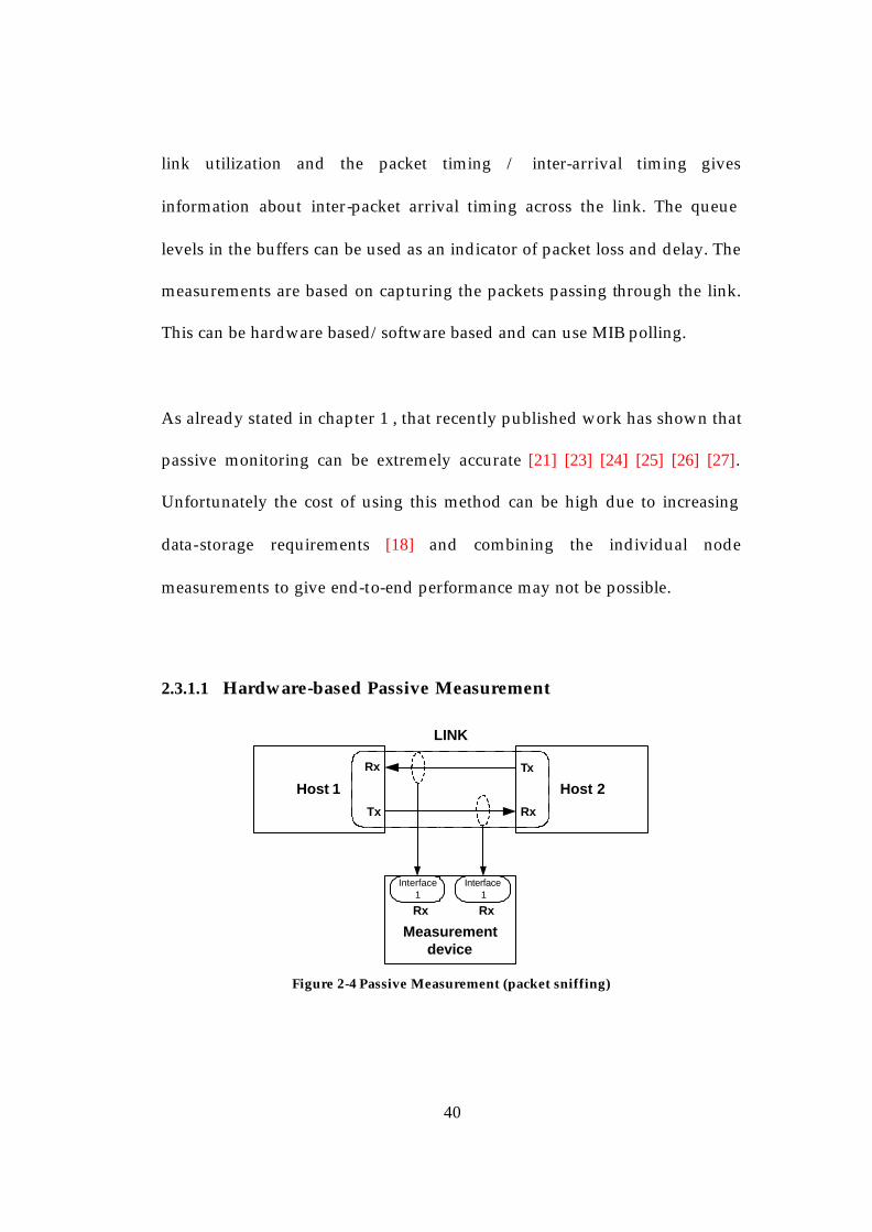
2.3.1.1 Hardware-based Passive Measurement
Host 1 Host 2
Rx
RxTx
Tx
Interface1
Interface1
LINK
Rx Rx
Measurementdevice
Figure 2-4 Passive Measurement (packet sniffing)

41
Figure 2-4 depicts the setup of an external Passive Measurement system for
packet monitoring. A part of the signal in the link passes to the
measurement device. This can be achieved by using an optical splitter for
fibre-optic network or a resistor network for copper media. The packets
passing through the link are captured by this measurement device, and used
to provide the set of information previously discussed.
2.3.1.2 Software-based Passive M easurement (Tcpdump) Tcpdump is a software-based monitoring application, which is supported
under most Unix systems. This program resides in the local node. It listens
on a specified network interface, and captures all traffic seen on that link. It
will dump all data sourced from and destined for that interface, as well as
any other traffic seen on that section of the network, and is not restricted to
TCP. Tcpdump can run in two modes:
• Capturing traffic to a file
• Displaying text information about every packet on the screen
However, without a special interface to the network, Tcpdump would be
unable to capture any packets that were destined for other machines or other
applications on the monitor. This would mean that passive measurement
would not be possible in such cases.

42
2.3.1.3 Polling MIB Measurement tasks can be performed in the local node e.g. queue length
monitoring [65]. Queue length monitoring has already been adopted in
schemes like Random Early Detection (RED) [66], in which the queue length
is monitored for every arriving packet and an Exponentially Weighted
Moving Average1 (EWMA) updated and this determines whether the
incoming packet should be dropped in order to avoid congestion.
Statistics like packet loss at the node/interface can be stored in management
objects like MIB. The MIB information is retrievable to the NOC with
management tools like SNMP as already discussed earlier. This process is
well known as MIB polling [67]. Taking Junpiter’s router’s MIB definition as
an example, the following MIB objects can be found [68]:
• Queued packet/byte statistics
o The total number of packets of specified forwarding class
queued at the output on the given interface
• Transmitted packet/byte statistics
o Number of packets of specified forwarding class transmitted
on the given interface
1 The average queue size is calculated using an EWMA of the queue size. At each arrival,i, the average queue size,qi, is updated by applying a weight,w, to the current queue size, ki.So, qi=wki + (1-w)qi-1
43
• Tail-dropped packet statistics
o The total number of packets of specified forwarding class
dropped due to tail dropping at the output on the given
interface
• RED-dropped packet statistics
o Total number of packets belonging to the specified forwarding
class dropped due to RED (Random Early Detection) at the
output on the given interface
2.3.2 Active Measurement
The main drawback of passive monitoring is that it requires full access to
network resources (e.g. routers, SNMP utilization) otherwise it is impossible
to combine into end-to-end QoS measures. For this reason Active Probing is
becoming the default means of network measurement, and a considerable
amount of recent work has concentrated on developing techniques for active
probing [28] [29] [30] [31] [32] [33].
Active measurement by probing is a means by which testing packets
(probes) are sent into the network. An example technology is the Cisco IOS
Service Assurance Agent (SAA) [58], which uses probe packets to provide
insight into the way customers’ network traffic is treated within the network.
Similarly, Caida and NLANR [35], [36] use probing to measure network
44
health, perform network assessment, assist with network troubleshooting
and plan network infrastructure. This is explained in detail in § 2.4.
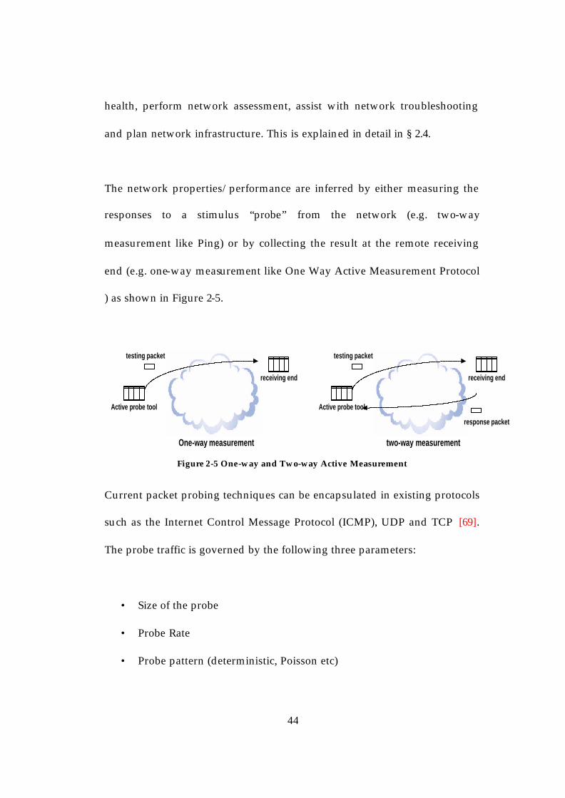
The network properties/performance are inferred by either measuring the
responses to a stimulus “probe” from the network (e.g. two-way
measurement like Ping) or by collecting the result at the remote receiving
end (e.g. one-way measurement like One Way Active Measurement Protocol
) as shown in Figure 2-5.
Active probe tool
receiving end
testing packet
Active probe tool
receiving end
testing packet
response packet
One-way measurement two-way measurement
Figure 2-5 One-way and Two-way Active Measurement
Current packet probing techniques can be encapsulated in existing protocols
such as the Internet Control Message Protocol (ICMP), UDP and TCP [69].
The probe traffic is governed by the following three parameters:
• Size of the probe
• Probe Rate
• Probe pattern (deterministic, Poisson etc)

45
A further consideration is that it is imperative that the measurements are
carried out over valid periods when the customers are active. Otherwise, the
performance statistics would be averaged over virtually unloaded periods
and would not then reflect an accurate picture [46].
Some typical Active Measurement tools are highlighted in the following
section.
2.3.2.1 PING The most widely used method to investigate e.g. network delay is for a
measurement host to construct and transmit an ICMP echo request packet to
an echo host. As the packet is sent, the sender starts the timer. The target
system simply reverses the ICMP headers and sends the packet back to the
sender as an ICMP echo reply. When the packet arrives at the original
sender’s system, the timer is halted and the elapsed time noted, i.e. the RTT
is calculated by the difference between the time the echo request is sent and
the time a matching response is received by the PING application [70]. Thus,
the end-to-end delay may be approximated by half of the time elapsed
between the testing packet sending time and the acknowledge packet
receiving time. This approach is being used in some ATM switches and some
IP network performance testing projects [70]. Figure 2-6 illustrates an ICMP
PING implementation.

46
Ping packet
Echo Packet
Ping packet
Echo Packet
Asymmetric Path Symmetric Path
Forward Path Forward Path
Return Path
Return Path
Figure 2-6 ICMP PING implementation
The basic applications of PING are as follows:
• To test the availability of a path between the source and destination
end
• To measure the RTT
Availability may be tested by the source “PINGing” the destination by
sending an ICMP’s echo request packet. If the destination is not reachable, a
Time Out will occur to indicate this event.
47
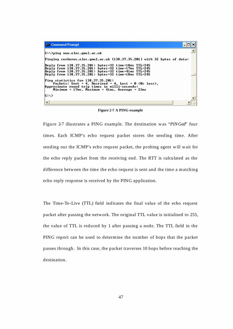
Figure 2-7 A PING example
Figure 2-7 illustrates a PING example. The destination was “PINGed” four
times. Each ICMP’s echo request packet stores the sending time. After
sending out the ICMP’s echo request packet, the probing agent will wait for
the echo reply packet from the receiving end. The RTT is calculated as the
difference between the time the echo request is sent and the time a matching
echo reply response is received by the PING application.
The Time-To-Live (TTL) field indicates the final value of the echo request
packet after passing the network. The original TTL value is initialised to 255,
the value of TTL is reduced by 1 after passing a node. The TTL field in the
PING report can be used to determine the number of hops that the packet
passes through. In this case, the packet traverses 10 hops before reaching the
destination.

48
2.3.2.2 Traceroute The Traceroute technique allows a measurement host to deduce the forward
path to the destination. Traceroute makes use of the TTL field in the IP
packet (which allows the maximum number of router hops the packet can
pass through before being dropped or returned) and ICMP control
messages. When the packet is dropped due to the expired TTL, the
information from the intermediate node will be returned to the
measurement host. A Traceroute example is illustrated in Figure 2-8.
Figure 2-8 A Traceroute example
Initially, the Traceroute application sends out three ICMP Traceroute
packets (with type number = 30) and TTL value = 1. After traversing the first
hop, the TTL value is decreased by 1 and so these Traceroute packets will be
dropped. The first node sends back the Time Exceeded Message back to the
measurement host with the node’s information. Therefore, the first node is
resolved. Then, another three ICMP’s Traceroute packets are sent out, but
the TTL value is increased to 2. For the same reason, these three ICMP

49
Traceroute packets will be dropped in the second hop, and the measurement
host will obtain the second node’s information based on the Time Exceeded
Message from this node. The TTL value of the Traceroute packets are
gradually increased until the full path is identified.
2.3.2.3 One-Way Active Measurement Protocol Recently, the Internet Engineering Task Force’s (IETF) Internet Protocol
Performance Metrics (IPPM) group proposed a new measurement protocol
called One-Way Active Measurement Protocol (OWAMP) [71] [29]. The
Active Monitoring tools (AMT) are intentionally placed at two measuring
points: sending and receiving ends. The AMT at the sending end generates
and injects the testing packets (probes) into the network, while the AMT at
the receiving end collects these probes for analysis.
Figure 2-9 IPPM One Way Active Measurement

50
Figure 2-9 shows the OWAMP architecture. There are two messages defined
in this protocol: OWAMP-Control and OWAMP-Test message. It is assumed
that both end-points are time synchronized. The client initiates a testing
session by sending an OWAMP-Control message to the server. In the
OWAMP-Control message, the length of the measuring period and the
sampling frequency are specified. The AMT then generates the time-
stamped testing packets (probes), and sends them to the remote reference
point. At the remote point, the probes are collected and the measurement
results sent back to the server. Finally the client fetches the result for
analysis from the server. The difference between ICMP-based Active
Measurement (PING and Traceroute) and OWAMP is that the latter targets
one-way measurement (i.e. measuring the forward path), whereas, in the
ICMP-based Active Measurement, both forward and return paths are
involved. In this thesis, the analysis of measurement is based on sampling of
queue overflow. The queues are assumed to be actively monitored to infer
the packet loss probability and this is fully explained in chapter 4.
2.4 Organizations Standardising Network Measurements
There are three broad organizations that are working on setting up
standards. These are described in the following section.
51
2.4.1 Internet Engineering Task Force (IETF)
The IETF [72] is a standardization body focused on the development of
protocols used in IP networks. The IETF consists of many working groups
but this thesis considers only the IPPM group as it is responsible for the
development of standard metrics like one-way loss and delay, [73] to
facilitate the communication of metrics to existing network management
systems. An Internet Standard document commences as an Internet Draft
which can be submitted by any individual or Working Group, WG by
simply following a guideline and sending any document to the Internet
Draft Editor, which will be available as an Internet Draft under the Internet
Draft directory (ftp://ftp.ietf.org/internet -drafts/) within several days.
However, Internet Drafts are not considered published documents and will
be automatically removed after six months. Standards are expressed in the
form of Requests for Comments (RFC). An RFC is a formal document
showing the result of the committee and reviews by parties. The final
version of the RFC becomes the Standard with no further comments or
changes permitted. Though the IETF issue their own documents in the form
of an RFC, many of the documents are taken by the Internet
Telecommunications Unit – Telecommunications sector (ITU-T) for issue as
their Recommendations too. The ITU-T is the only international body

52
responsible for the telecommunications Standards. The ITU-T Y.1541 [48]
and G.711 [74] Recommendations have been used as references in this
research.
The IETF’s IPPM Working Group has the aim of developing a set of
Standard metrics for quantitative measurement of performance of Internet
data delivery services. These metrics will be designed such that they can be
performed by network operators, end users or independent testing groups.
The metrics already completed and published are connectivity, one-way
delay and loss, delay variation, loss patterns, packet reordering, bulk
transport capacity and link bandwidth capacity. Each of the documents
defines the metrics and the procedures to actually measure it. Another goal
of this IPPM Working Group is to produce documents that describe how the
above mentioned metrics characterise features that are important to different
service classes. Each document will discuss the performance characteristics
such as loss, delay, connectivity etc that are pertinent to a specified service
class identifying the set of metrics that describe them and the methodologies
necessary to collect them [73].
Current work of the IPPM reporting MIB focuses on the production of a MIB
to retrieve the results of IPPM metrics to facilitate the communication of
metrics to existing network management systems, and on the definition of a

53
protocol to enable communication among the test equipment that will
implement the one-way metrics [73].
The following are the Internet Drafts and the RFCs produced by this IPPM
Working Group:
• Internet Drafts:
1. A One-Way Active Measurement protocol (OWAMP)
2. Packet Reordering Metric for IPPM
3. Overview of Implementation reports relating to IETF work on IP
Performance Measurements (IPPM, RFC 2678 -2681)
4. Defining Network Capacity
5. A Two-Way Active Measurement Protocol (TWAMP)
6. IP Performance metrics (IPPM) for spatial and multicast
• Requests for Comments RFC:
1. Framework for IP Performance Metrics (RFC 2330)
2. IPPM Metrics for Measuring Connectivity (RFC 2678)
3. A One-Way Delay metric for IPPM (RFC 2679)
4. A One-Way Packet Loss Metric for IPPM (RFC 2680)
5. A Round-trip Delay Metric for IPPM (RFC 2681)
6. A Framework for Defining Empirical Bulk transfer Capacity metrics
(RFC 3148)

54
7. One-Way Loss Pattern Sample Metrics (RFC 3357)
8. IP Packet Delay Variation Metric for IPPM (RFC 3393)
9. Network Performance Measurement for periodic streams (RFC 3432)
10. A One-Way Active Measurement Protocol Requirements (RFC 3763)
11. IP Performance metrics (IPPM) metrics registry (RFC 4148)
2.4.2 Cooperative Association for Internet Data Analysis
(CAIDA)
CAIDA is located at UCSD (San Diego) and is collaboratively undertaking
among organizations in the commercial, government, and research sectors
aimed at promoting greater cooperation in the engineering and maintenance
of a robust, scalable global Internet infrastructure. As a part of CAIDA’s
mission to promote cooperative measurement and analysis of Internet traffic
and performance, collection of data for scientific analysis of network
function is one of CAIDA’s core objectives. CAIDA collects several different
data types at geographically and topologically diverse locations, and makes
this data available to the research community to the extent possible while
preserving the privacy of individuals and organisations who donate data or
network access. CAIDA collects information on availability of the Internet
and TCP/IP measurement tools as well as network visualization resources.
Its main goals are as follows [35]:

55
• Encourages the creation of Internet traffic metrics (in collaboration
with IETF/IPPM and other organizations)
• Works with industry, consumer, regulatory and other representatives
to assure their utility and universal acceptance.
• Creates a collaborative research and analytic environment in which
various forms of traffic data can be acquired, analyzed and (as
appropriate) shared.
• Promotes the development of advanced methodologies and
techniques for traffic performance and flow characterization,
simulation, analysis and visualization. Specific areas of future impact
include real-time routing instability, diagnosis and evolution for next
generation measurement and routing protocols (multicast and
unicast).
CAIDA also offers several tools for actively or passively measuring Internet
traffic and flow patterns such as [35]:
• Autofocus
• Beluga
• Cflowd
• Coral Reef
• Iffinder
• Mantra
56
• NetraMet
• RTG
• Scamper
• Skitter
Caida's Active Measurement Project includes real-time data reports
showing, among other things, packet loss rates between pairs of nodes. The
nodes concerned are in the US, largely at NLANR’s National Science
Foundation (NSF) supported High Performance Computing (HPC) sites
which are discussed in detail in the next section.
2.4.3 National Laboratory for Applied Network Research
(NLANR)
The U.S NLANR funded by the U.S NSF provides engineering, traffic
analysis, and technical end-user support for NSF HPC sites and high-
performance network service providers such as the vBNS and Abilene
networks.
NLANR is a distributed organization with three parts:
1. Application/User Support:
The Distributed Applications Support Team (DAST) offers support for
researchers working with high-performance network applications and

57
assists in the development of distributed applications and tools. Networking
assistance to campus network engineers, gigapop operators, and other high-
performance networking professionals is provided by NLANR's Engineering
Services staff [36].
2. Engineering Services:
The Engineering Services team provides in-depth information and
technical support for connecting to and effectively using high-
performance wide-area networks to campus network engineers,
operators and other high-performance networking professionals [36].
3. Measurement and Analysis:
The Measurement and Network Analysis (MNA) group of NLANR
assesses the performance of the next-generation computer networks,
measuring the flow of message traffic, analyzing performance issues, and
making all the data, analysis and tools available to the community so that
they can be tuned for maximum end-to-end performance [36].

58
NLANR/MNA research has two main components: Passive
Measurement and Analysis (PMA) project and the Active Measurement
Project (AMP). The PMA project uses information collec ted from
observing network traffic, without interacting with the networks
themselves. On the other hand, the AMP performs site-to-site active
measurements and analysis, which enable network researchers and
engineers to track problems and changes in network performance, by
inserting test messages into the networks and studying and observing
their progress through the systems [36]. AMP makes two-way
measurements using the ICMP PING facility and Traceroute which
includes RTT, packet loss, throughput and route information. The former
PINGs each other machine, once per minute and all the packet’s RTT and
losses are recorded. The latter occurs between all the host’s machines to
route from each machine to every other. Due to the asymmetric nature of
the Internet, measurement results using two-way measurement may
reduce the measurement accuracy as discussed earlier. That is why
NLANR has proposed a new protocol Internet Protocol Measurement
Protocol (IPMP) which was standardised by the IETF. IPMP allows
Internet devices to insert time stamps into data as it moves through the
network and therefore provides router-support for one-way delay
measurements. This approach improves the accuracy of the final time

59
stamp and hence the delay measurement, but the packet loss is hard to
measure accurately using PING.
The NLANR/MNA is developing a Network Analysis Infrastructure
(NAI) that is intended to provide both engineering and research support
for the High Performance Connection (HPC) community. Specifically, the
goal of the NAI project is to create an infrastructure that will support
measurements and analysis through the collection and publication of raw
data, visualisation and analysis of network measurement [75]. Currently
the main focus is on:
• Passive collection of header traces
• Active Measurement
• SNMP derived data
• BGP router based data
• Presenting the results of analysis to the HPC community
2.5 Applications of Network Measurements In the previous sections, network measurement methods and their
application from the industry’s point of view, has been discussed. This
section is organised according to the “technology” that the measurements
are applied to.
60
2.5.1 Network Tomography
The end systems can have problems in accessing the internal network
characteristics when the internal network element is owned by other
network providers or in an inter-network domain. To address this problem,
end-to-end measurements are performed and used to infer the internal
network elements’ characteristics, such as the loss characteristic [76] [77] or
the delay distribution in an intermediate node [78] [79] using a technique
called Network Tomography.
[80] addresses network tomography methods, based on end-to-end
measurements using active, multicast probing to gather packet correlation
statistics. The tomography is then used to infer internal network
characteristics. However, these probing methods require special support
from the network in terms of multicast capability (which most networks do
not currently support). Moreover, multicast-based methods may not provide
an accurate characterization of the network behavior, because routers treat
multicast packets differently to unicast packets. In contrast to multicast
techniques, unicast network tomography is easily carried out on most
networks and is scalable. Unicast methods [81] will also provide more
accurate estimates of network behavior, since the traffic in most networks is

61
predominantly unicast in nature. Tomography needs accurate
measurements, it does not provide them.
2.5.2 Measurement-based Admission Control
The role of an admission control algorithm is to ensure that the admission of
a new connection into a resource constrained network does not violate
service commitments made by the network to the admitted flows, whilst
maintaining good network utilization. One of the approaches to admission
control is known as parameter-based, which computes the amount of
network resources required to support a set of flows given a priori flow
characteristics. The new connection will not be accepted if the network
resource is not sufficient. The main problem of parameter-based admission
control is the difficulty of a priori flow characteristic estimation [82]. It is
difficult to accurately estimate the traffic parameters when a flow is yet to be
established. Inaccurate assumption of the traffic information may result in
service degradation for other, existing, flows. Guaranteed QoS performance
can certainly be ensured by using worst -case traffic characteristics (e.g. using
the peak rate), but this will surely lead to the network’s under-utilization
[83].

62
Much research work has been carried out to study an approach called
Measurement-based Admission Control (MBAC) which avoids the problem
faced by the parameter-based algorithm, by shifting the task of traffic
specification from the application to the network, so that admission
decisions are based on traffic measurements instead of explicit specification.
Different end-to-end schemes [84] [85] [86] [87] [88] [89] [90] [91] [92] [93]
[94] [95] [96] [97] [98] [99] have been proposed to support QoS for
applications (e.g VoIP) [100] [101]. Thus, MBAC can achieve much higher
network utilization than parameter-based algorithm while still providing
acceptable SLAs.
[102] proposed an end-to-end MBAC mechanism for VoIP networks. In
[102], active measurement is used for call admission control to maintain
packet loss rate for voice flows below a pre-determined value under various
network conditions. This method, unlike Passive measurement, is very
useful when using in large-scale VPN networks where the VPN is carried
over a heterogeneous mixture of packet networks, not owned by any single
organization.
2.5.3 Available Bandwidth Estimation
The available bandwidth of a network path is the maximum throughput that
the path can provide for a new flow without significantly reducing the

63
throughput of the cross traffic along the path [103]. Available bandwidth is
of great importance for various network applications and hence knowledge
of the available bandwidth on an end-to-end path can improve end-to-end
admission control [103], congestion control [104] as well as service level
agreement verification [105]. Customers should be able to verify, with their
own measurements, that they indeed get the bandwidth that they pay for.
Measurement tools that can measure the path’s available bandwidth are of
major importance for NSPs.
Obtaining useful estimates of the available bandwidth from routers is often
not possible due to various technical and privacy issues or due to an
insufficient level of measurement resolution or accuracy. Thus, it becomes
necessary to infer the required information from the network edge via
Active measurement.
Current schemes for available bandwidth estimation fall into two broad
classes. The first class of schemes is based on statistical cross-traffic models,
also known as Probe Gap Model (PGM) such as Delphi [106] and Initial Gap
Increasing (IGI) [107]. PGM exploits the information in the time gap between
the arrivals of two successive probes at the receiver. A probe pair is sent
with a time gap in∆ , and reaches the receiver with a time gap out∆ .
Assuming a single bottleneck and that the queue does not become empty
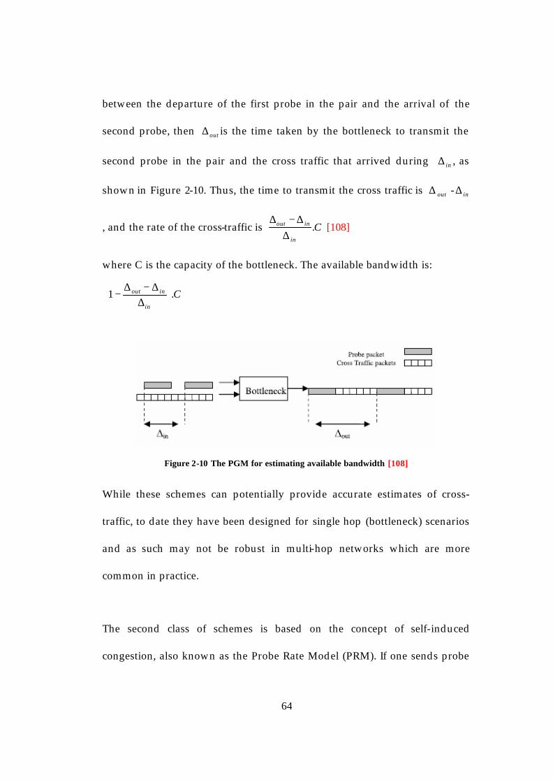
64
between the departure of the first probe in the pair and the arrival of the
second probe, then out∆ is the time taken by the bottleneck to transmit the
second probe in the pair and the cross traffic that arrived during in∆ , as
shown in Figure 2-10. Thus, the time to transmit the cross traffic is out∆ - in∆
, and the rate of the cross-traffic is Cin
inout .∆
∆−∆ [108]
where C is the capacity of the bottleneck. The available bandwidth is:
Cin
inout .1
∆
∆−∆−
Figure 2-10 The PGM for estimating available bandwidth [108]
While these schemes can potentially provide accurate estimates of cross-
traffic, to date they have been designed for single hop (bottleneck) scenarios
and as such may not be robust in multi-hop networks which are more
common in practice.
The second class of schemes is based on the concept of self-induced
congestion, also known as the Probe Rate Model (PRM). If one sends probe
65
traffic at a rate lower than the available bandwidth along the path, then the
arrival rate of probe traffic at the receiver will match their rate at the sender.
In contrast, if the probe traffic is sent at a rate higher than the available
bandwidth, then queues will build up inside the network and the probe
traffic will be delayed. As a result, the probes' rate at the receiver will be less
than their sending rate. Thus, one can measure the available bandwidth by
searching for the turning point at which the probe sending and receiving
rates start matching. Examples of the self-induced congestion approach are
pathload [108], pathChirp [109] and TOPP [110]. This is not the best method
as it is congesting the network to try to measure the available bandwidth
which is then affected by the process of measurement.
2.6 Summary This chapter has reviewed network measurement techniques from different
aspects: the motivation, different measurement approaches, features of the
measurement methods and their applications. It has also highlighted
research which is network measurement based. The motivation for network
measurement comes from the need for network performance assessment or
monitoring. Performing network measurements allow the operator to collect
the useful data for analysis or assessment. A variety of network
measurement based techniques have been proposed and developed, but
they can be classified into two broad classes: Active Measurement and

66
Passive Measurement. Examples of Active Measurement tools are Ping,
Traceroute or OWAMP, whereas packet sniffing, tcpdump and polling MIB
are typical examples of Passive Measurement tools.
67
3 End-to-End Packet Loss Issues
This chapter focuses on the importance of end-to-end packet loss, its effect
on applications like VoIP and describes the analyt ical model.
3.1 Why is Loss Important? IP and MPLS packet networks are now carrying a heterogeneous mix of
traffic, with widely differing QoS requirements. The service model of
emerging multi-service packet networks, including the packet backbones for
2.5Generation (G) and 3G mobile networks, is based on the network’s ability
to guarantee QoS to user applications [38]. End-to-end packet loss is one of
the most significant QoS performance metrics available in SLAs because for
many applications e.g. VoIP, the performance drops drastically if the end-to-
end loss exceeds a certain limit, and will become unusable under excessive
loss.
3.1.1 UDP and TCP based applications
The network layer is responsible for delivering packets to any destination
node within the network, and consequently the routing of packets is one of
the tasks of its protocols. IP is used by the two main protocols of the
transport layer, UDP and TCP, both providing packet flows between two
hosts for application layer protocols. There is a significant difference
between these two protocols. While TCP provides a reliable flow of packets,

68
the much simpler UDP only transmits packets but does not guarantee their
delivery. UDP is used for example by applications like the Simple Network
Management Protocol (SNMP) and the Network Time Protocol (NTP), while
TCP is used by the File Transfer Protocol (FTP) and Simple Mail Transfer
Protocol (SMTP).
Loss can have a significant impact on the performance of both TCP and UDP
based applications. Email for example, may involve text and still images and
the performance degradation caused by losses can be corrected by
retransmitting the packets with the help of TCP. But re-transmissions
gradually increases the load, so increasing the loss and hence the number of
re-transmissions [50]. However, for UDP based applications, like VoIP,
timely packet delivery and packet ordering is important. Packets must reach
the destination within a bounded time period [50]. VoIP has the advantage
of not requiring a completely reliable transport level, although it does need
real-time delivery. The loss of a packet or a single bit error will often only
introduce a “click” or a minor break in the voice output.
Some applications already possess internal probing like Real-Time Control
Protocol/ Real-Time Protocol (RTCP/RTP), where RTCP is used in VoIP
signalling and RTP is used to send and receive the voice signal. However, as
IP networks may route packets via different pathways to their destination,

69
RTP packets may arrive out-of-order, or be delayed or lost. That is why
RTCP is not widely implemented [111] and is not considered in this thesis.
Many businesses are dependent on distributed, networked computing
systems and are beginning to rely on high-speed communications for
multimedia interactions and Web-based services. Users are now requiring
access to these services while travelling. In addition, new multimedia
applications are emerging for Web enabled telephones and mobile
computers with integrated communications. Multimedia applications
require more sophisticated management of these system components, which
affect the QoS delivered to users. This means that customers will require
SLAs that are genuine, monitored and enforceable guarantees.
Thus, NSPs should be able to differentiate these different applications (TCP,
UDP) into classes so that their QoS needs can be managed. The ITU-T
proposes grouping IP telecommunications transactions into six classes
defined according to the desired performance objectives. According to this
recommendation, ‘a packet flow is the traffic associated with a given
connection or connectionless stream having the same source host,
destination host, and class of service and session identification.
Recommendation Y.1574, summarized in Table 3-1 [48], specifies a PLP of
less than 10-3 (where a PLP is specified).

70
Table 3-1 Classes of Service (CoS) [48]
3.2 Causes of Packet Loss There are two major causes of packet loss in IP networks. One is congestion,
where the network routers/switches are temporarily sent more packets than
their buffers can accommodate. The other is due to link failure, when all the
bits currently in transit on that link will be lost. Further packets that are also
transmitted down the broken link will be lost until the Synchronous Digital
Hierarchy (SDH) layer reconfigures a new route around the failed link. Link
71
failure is not considered in this thesis.
The effect of packet loss on the user depends mainly on the following three
factors:
• Packet Loss Rate
• Packet Loss Distribution
• Packet Size ( larger packets contain more information)
Packet loss due to congestion is a fundamental problem in managed IP
networks. A queue forms in a buffer until the router is able to transmit them
on their way. In this thesis, it is considered that buffer overflow takes place
when a queue exceeds its buffer limit i.e tail-drop queues. Random Early
Discard (RED) mechanisms cause packet drop before the buffer is full. These
mechanisms are not considered in the main part of the research reported in
this thesis. However, it is discussed in § 7.2.
3.3 Traffic Models
Queueing behaviour in a buffer is powerfully affected by the ‘arrival’
process. Traffic models have long been used to mimic the real network
traffic. This section highlights some of the most useful traffic models and
discusses their use for mimicking real queueing behaviour. An accurate
traffic model can assist the network performance analysis either through
72
analytical techniques or computer simulations. A good traffic model should
be able to capture the key characteristics of the actual traffic in as
parsimonious a fashion as possible. If the traffic models do not accurately
represent actual traffic closely enough, one may overestimate or
underestimate the network performance. In this section, we review some of
the well-recognized traffic models [84], ultimately focusing on the On/Off
traffic model as most appropriate for use in the research reported in this
thesis.
Traffic models may be divided into many different classification schemes
like Fractional Gaussian Motion and Fractional Brownian Motion but in this
thesis the focus is on the exponential On/Off model for short-range
dependent (SRD), and a similar On/Off model with Pareto distributed
sojourn times to feature long range dependent (LRD). These are discussed in
the next section.
3.3.1 Short-Range Dependent Traffic Models
The first performance models for telecommunication systems were based on
the assumption that packet arrival processes follow a Poisson process [44]
[113] [114]. Subsequently, Markov Modulated processes have been
introduced representing a variety of traffic scenarios. In this section, we
review their variants.

73
3.4.1.1 Interrupted Poisson Process (IPP) Models
Figure 3-1 IPP model
Figure 3-1 depicts an IPP traffic model. IPP is also a two-state model with
two states: ON and OFF. The time spent in ON and OFF states is
exponentially distributed with mean 1/α and 1/β respectively. Arrivals only
occur in the ON state, and do so according to a Poisson distribution with
rate, λ.
3.4.1.2 Markov modulated Poisson process (MMPP)
Figure 3-2 Superposition of N voice sources
Figure 3-2 depicts an MMPP model for multiplexed voice. This process is
extensively used to model aggregate network traffic [115] [116]. This process
ON OFF
α
β
λ
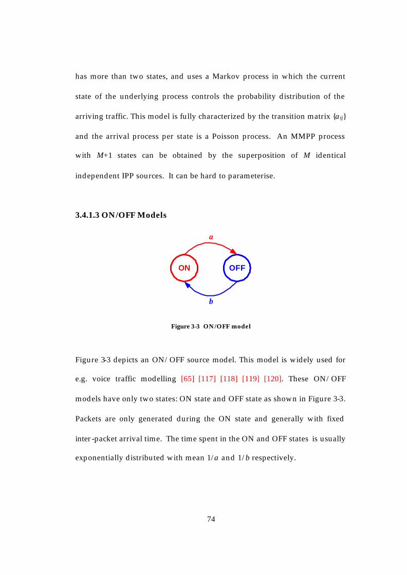
74
has more than two states, and uses a Markov process in which the current
state of the underlying process controls the probability distribution of the
arriving traffic. This model is fully characterized by the transition matrix {αij}
and the arrival process per state is a Poisson process. An MMPP process
with M+1 states can be obtained by the superposition of M identical
independent IPP sources. It can be hard to parameterise.
3.4.1.3 ON/OFF Models
ON OFF
α
β
Figure 3-3 ON/OFF model
Figure 3-3 depicts an ON/OFF source model. This model is widely used for
e.g. voice traffic modelling [65] [117] [118] [119] [120]. These ON/OFF
models have only two states: ON state and OFF state as shown in Figure 3-3.
Packets are only generated during the ON state and generally with fixed
inter-packet arrival time. The time spent in the ON and OFF states is usually
exponentially distributed with mean 1/α and 1/β respectively.
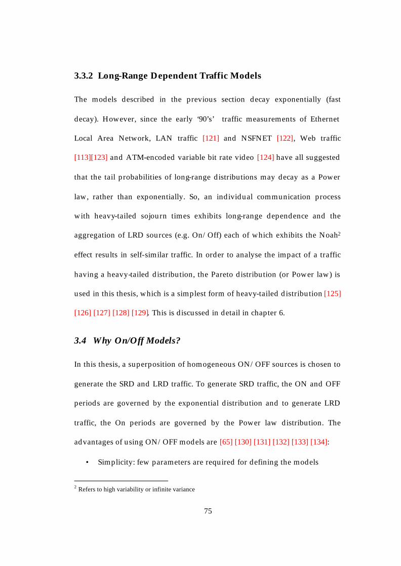
75
3.3.2 Long-Range Dependent Traffic Models
The models described in the previous section decay exponentially (fast
decay). However, since the early ‘90’s’ traffic measurements of Ethernet
Local Area Network, LAN traffic [121] and NSFNET [122], Web traffic
[113][123] and ATM-encoded variable bit rate video [124] have all suggested
that the tail probabilities of long-range distributions may decay as a Power
law, rather than exponentially. So, an individual communication process
with heavy-tailed sojourn times exhibits long-range dependence and the
aggregation of LRD sources (e.g. On/Off) each of which exhibits the Noah2
effect results in self-similar traffic. In order to analyse the impact of a traffic
having a heavy-tailed distribution, the Pareto distribution (or Power law) is
used in this thesis, which is a simplest form of heavy-tailed distribution [125]
[126] [127] [128] [129]. This is discussed in detail in chapter 6.
3.4 Why On/Off Models?
In this thesis, a superposition of homogeneous ON/OFF sources is chosen to
generate the SRD and LRD traffic. To generate SRD traffic, the ON and OFF
periods are governed by the exponential distribution and to generate LRD
traffic, the On periods are governed by the Power law distribution. The
advantages of using ON/OFF models are [65] [130] [131] [132] [133] [134]:
• Simplicity: few parameters are required for defining the models
2 Refers to high variability or infinite variance
76
• A basic prototype for a bursty traffic source
• An effective model used for mimicking packet traffic
• Known parameters for VoIP
To model traffic by using aggregate ON/OFF source, only a few parameters
are needed compared with other traffic models like the MMPP. The
parameters needed for ON/Off sources include the number of the aggregate
sources, the packet transmission rate in the ON period and the parameters
defined in the distributions for the ON and OFF periods. If exponential
distributions are employed for the ON/OFF periods, then the mean ON time
and mean OFF time are sufficient.
ON/OFF behaviour is the basic nature of packet traffic. For example, with
voice traffic, packets are generated when the user is in an active state (ON),
whereas, in the silent state (OFF), a small number of packets, or no packets,
are generated, and the process alternates between ON and OFF state.
Another example of ON/OFF type behaviour can be found in Web traffic.
Users download the web-page information which is equivalent to the ON
state, and then the model can switched to an OFF state while the user is
browsing this web-page. An ON/OFF source is the basic prototype for a
bursty source and has been used extensively in traffic modelling [130] [135]
[136] [137] [138] [139].

77
3.5 Queueing Behaviour for a FIFO Buffer Multiplexing
Markovian Traffic
A variety of detailed studies have been performed on packet queue
behaviour under various traffic and load conditions. These studies have
taken place over many years [65] [44] [140] [141], and have concluded that a
reliable model exists for the buffering of the packets under general
“Markovian” conditions.
Figure 3-4 Queueing Behaviour for a FIFO multiplexing Markovian Traffic
Figure 3-4 depicts the typical queue length distribution “shape” for a FIFO
queue multiplexing Markovian traffic. With reference to Figure 3-4, the
queue length distribution consists of two regions, often referred to as packet-
scale region and burst-scale region [65] [44]. The queue length distribution
starts with the packet scale component with a steeper slope. The
distribution then gradually changes to a second branch with a flatter slope,

78
the burst scale component. The intersection of the tangents to both branches
is often designated as the “knee” point. The qualitative explanation of this
behaviour is given in Appendix A of this thesis.
For a FIFO queue multiplexing Markovian traffic, the important feature of
the burst-scale queuing and the packet-scale queuing components are their
exponential decay, i.e. they approximately follow a straight line in log-linear
scale [65]. This widely accepted and understood model is the key to the
analysis developed in this thesis for the accuracy of packet loss monitoring.
This thesis concentrates mainly on VoIP traffic [50] [74] [142] [143] [144] [145]
[146] as:
• It is very common
• It has tight and well understood loss and delay requirements
• It has a well accepted traffic model, an On/Off source, with agreed
parameters, making studies by analysis and simulation acceptable.
The VoIP multiplexing model is discussed in more details in chapter 4.
3.6 Summary
This chapter discussed the causes of packet loss: link failure and buffer
overflow. It also discusses the different types of traffic models relevant to

79
this research: short range dependent traffic and long range dependent traffic.
It discussed the choice of model used in this research: the On/Off model.
Finally, it highlighted the queueing behaviour for a FIFO buffer multiplexing
Markovian traffic where the queue length distribution consists of two
regions, often referred to as packet-scale region and burst-scale region.

80
4 Overflow Analysis for Single Buffered Links
This chapter reviews the basic queue model adopted in this research, and
applying results from simulation and analysis, examines the effectiveness of
probing for packet loss probability through a buffered access link. Access
link utilization during busy hours has been found often be in the 70%-80%
load range [16] [19]. It is well known, that, currently, access links are the
network bottleneck.
4.1 The Loss Model for a Buffered Link
The model consists of N On/Off sources that are multiplexed through a
buffer with a single output link of bandwidth, C, as depicted in Figure 4-1a.
The On/Off Traffic Model was described in chapter 3. The aggregated input
rate for a period, must be greater than the shared output link rate, C, in
order for a queue to grow, and ultimately loss to take place.
Figure 4-1b is an illustration of how the occupancy of a buffer in a router
might evolve over time. Congestion occurs when the aggregate sending rate
of the N On/Off sources exceeds the capacity of the shared output link for a
sufficient period of time. This is illustrated as a positive slope in the queue
length graph. The rate of increase of the queue length depends both on the
number of active On/Off sources and on the sending rate of each source. A

81
loss episode begins when the aggregate sending rate has exceeded C for a
period of time sufficient to fill the buffer (e.g. at times a and c in Figure 4-1b).
A loss episode ends when the aggregate sending rate drops below C and the
buffer begins a consistent drain down (e.g. at times b and d in Figure 4-1b).
A loss period is defined as the difference between start and end times (i.e. ‘b-
a’ and‘d-c’). A buffer will go through a number of cycles where each cycle is
defined as having a mean duration of Tcycle and consisting of an overflow
period of mean duration A secs followed by a non-overflow period of mean
duration A’ secs [19] [29].
Figure 4-1 Loss Model

82
It is a critical aspect that drives the work presented in this thesis that the loss
periods that result from multiplexing On/Off sources are themselves bursty.
This means that loss episodes are comparatively rare, but when they do
occur, they may see a very large number of packets lost, virtually
consecutively [19] [44].
VoIP traffic for example reinforces the intuition about the importance of the
packet loss pattern. When lost packets occur together, in a burst, the audio
effect for the users is significantly worse than when packets are lost one at a
time. This is because bursty packet loss results in a larger segment of speech
being lost or distorted, causing impairment that is much more noticeable to
users. Furthermore, the larger the segment lost, the harder it is to cover up
or conceal [50].
4.2 Loss Cycle Time Analysis
The analysis focuses on a homogeneous mix of N Markovian ON-OFF traffic
sources multiplexed into a single packet buffer as discussed in § 4.4. As in
many previous analyses [19] [44] [147], a form of analysis is used here that
was designed specifically for multiplexing N On/Off sources. This technique
[44] simplifies the N ON/OFF sources to a single aggregate ON/OFF source,
reducing the state space from 2N possible states to just 2, and simplifying the
analysis while retaining accuracy as illustrated in Figure 4-2.
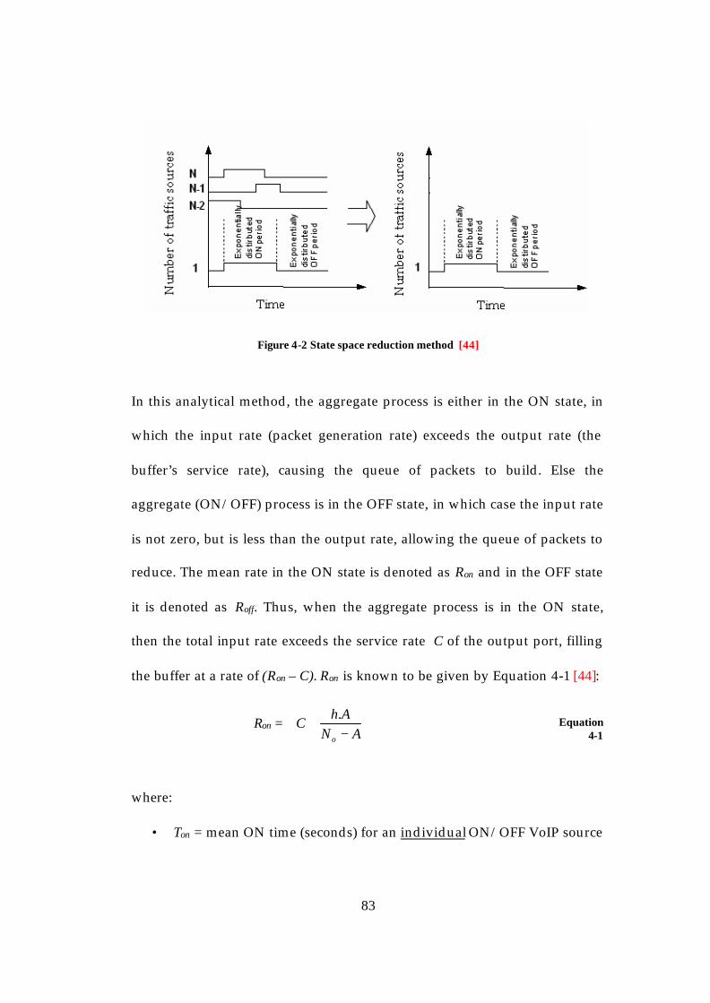
83
Figure 4-2 State space reduction method [44]
In this analytical method, the aggregate process is either in the ON state, in
which the input rate (packet generation rate) exceeds the output rate (the
buffer’s service rate), causing the queue of packets to build. Else the
aggregate (ON/OFF) process is in the OFF state, in which case the input rate
is not zero, but is less than the output rate, allowing the queue of packets to
reduce. The mean rate in the ON state is denoted as Ron and in the OFF state
it is denoted as Roff. Thus, when the aggregate process is in the ON state,
then the total input rate exceeds the service rate C of the output port, filling
the buffer at a rate of (Ron – C). Ron is known to be given by Equation 4-1 [44]:
Ron =
−
+AN
AhC
o
. Equation
4-1
where:
• Ton = mean ON time (seconds) for an individual ON/OFF VoIP source

84
• C = the output capacity of the buffer (link capacity), in packets per
second
• h = ON rate of an individual ON/OFF VoIP source
• Ap = mean packet arrival rate to the buffer in packets per second.
A is the total offered traffic in terms of packet flows
= h
AA p Equation
4-2
No is the maximum number of packet flows that can be served
simultaneously
( )hCN o = Equation
4-3
The ON rate in the ON state is [44]:
Ron =
−+
p
p
AC
AhC
. Equation
4-4
The mean time the aggregate process spends in the ON state is denoted as
T(ON), and this is given by Equation 4-5. This can [19] [44] be used as a very
accurate estimator for the mean duration of a buffer overflow period, E(OF):
E(OF) ˜ T(ON) =
− p
on
ACTh. Equation
4-5

85
This is because sojourn time in aggregate On state is modeled as an
exponential distribution as illustrated in Figure 4-2 and therefore the mean
in ‘a’ , T(ON) is the same as ‘b’, E(OF) due to the “Memoryless” property of
the exponential distribution. This has been published in [19] and further
details are in Appendix B.
Figure 4-3 Sojourn time in aggregate ON state
Since the aggregate On period is exponentially distributed and the aggregate
arrival rate is fixed to Ron, there is a Geometrically distributed number of
packet arrivals during an aggregate ON period. From this observation, it can
be seen that the mean number of excess-rate packets in an ON period is the
product of the mean duration in the ON state, T (ON) and the excess rate,
(Ron-C). Thus, the expected number of packets lost per overflow period, pµ ,
for a single buffered link is given by
( ) )(. ONTCRonp −=µ Equation 4-6

86
( )2
2 ..
p
ponp AC
ATh
−=µ Equation
4-7
This section develops an analytical technique to approximate the mean time
to lose a probe, µt, accounting for the burstiness of the overflow (loss)
process. The main contributor to this time period is that a queue in a buffer
will go through a number of cycles, where each cycle has a mean duration of
Tcycle and consists of an overflow period of mean duration A secs followed by
a non-overflow period of mean duration A’ secs [29] as already mentioned in
§ 4.2. The probe stream may have to go through a series of these cycles
before encountering an overflow period that will lead to a loss. It can be seen
that
p
cyclepcycle A
NT /= Equation
4-8
where Np/cycle is the mean number of packets in one cycle.
Since cyclep
p
NPLP
/
µ=
It can be seen that
( )2
2
..
p
oncycle ACPLP
ThT
−= Equation
4-9

87
Tcycle can be used as a lower bound on the time to encounter (with a probe)
an overflowing buffer as shown in Figure 4-4.
Figure 4-4 Lower bound for the mean cycle time
4.3 Analysing the interaction between the probe stream and the
buffer overflows
In reality, probing is complicated by the fact that the stream of probes may
miss an overflow period completely, as illustrated in Figure 4-5. This
occurrence is most likely when T(ON) is noticeably smaller than the inter-
probe time. Further to this, as the duration of the overflow periods are
random, this can still happen even when the mean overflow period is long
w.r.t. the inter-probe time.
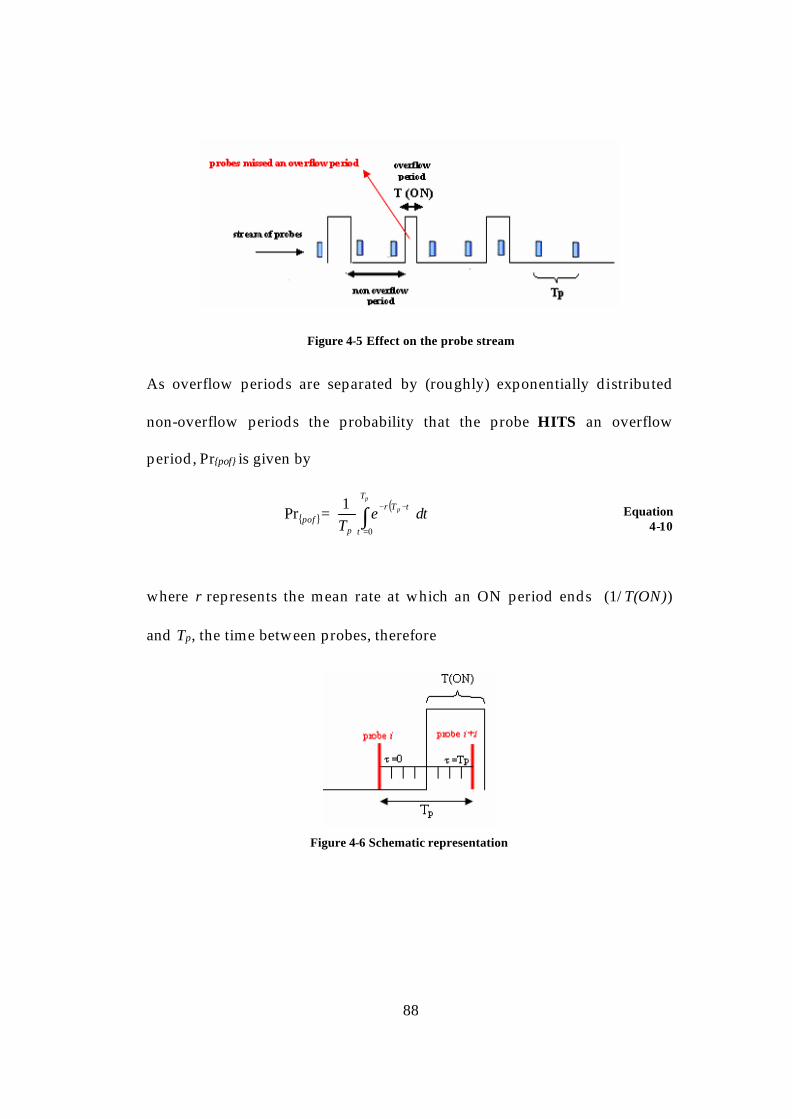
88
Figure 4-5 Effect on the probe stream
As overflow periods are separated by (roughly) exponentially distributed
non-overflow periods the probability that the probe HITS an overflow
period, Pr{pof} is given by
{ }pofPr = ( ) ττ
τ deT
p
p
TTr
p∫=
−−
0
1 Equation
4-10
where r represents the mean rate at which an ON period ends (1/T(ON))
and Tp, the time between probes, therefore
Figure 4-6 Schematic representation

89
( )τ−− pTre is used because exponential follows the format te λ− where λ is the
arrival rate and t is the time. Likewise, r is the overflow period completion
rate:
(1/T(ON) ) = 1/(E(OF)) where E(OF) is the mean overflow period duration,
and ( )τ−pT is the time. Since, the aim is to find the probability that a probe
hits an overflow period, the time a probe hits an overflow period is divided
by the total inter-probe time, pT (Figure 4-6).
{ }
( ) ( )
( )
p
p
T
TONT
ppof
ONT
eT
0
.1
11Pr
=
−−
−=
τ
τ
Equation
4-11
{ }( ) ( ) ( ) ( ) ( ) ( )
−−
−=−
−−
−ppp TT
ONT
p
TONT
ppof e
TONTe
TONT
10
1
Pr Equation
4-12
{ }( ) ( ) ( )
−−
−=
−
1Pr xTONTe
TONT
p
ONT
T
ppof
p
Equation
4-13
{ }( ) ( )
−=
−
ONT
T
ppof
p
eTONT 1Pr
Equation 4-14
{ }
( ) ( )
( )
p
p
T
TONT
ppof
ONT
eT
0
.1
11Pr
=
−−
−=
τ
τ
Equation
4-15

90
Since ( )
−=
p
on
ACTh
ONT. so substituting T(ON) into Equation 4-16 gives:
( )
−
−=
−−
on
pp
Th
TAC
p
on
p
eAC
ThT
.
.
{pof} 1.1
Pr Equation
4-16
So, the probability for the probes to MISS an overflow period will be (1-
Pr{pof})
P(miss) = 1 - ( )
−
−
−−
on
pp
Th
TAC
p
on
p
eAC
ThT
.
.
1.1 Equation
4-17
The mean of the Geometric distribution for the number of probes missing an
overflow period, mγ is 1/P(miss) as shown below:
( )
−
−−
=−−
on
pp
Th
TAC
p
on
p
m
eAC
ThT
.
.
1.1
1
1γ Equation
4-18
The expected time until a probe encounters an overflowing buffer is
calculated from the mean number of “attempts” (probes) until a probe
“succeeds” in being lost due to buffer overflow, which is by definition the
mean number of cycles until this occurs. Therefore Equation 4-19 shows the

91
full derived expression for the mean time until a probe is lost (µt) due to an
overflowing buffer.
cyclemt T.γµ = = ( )
−
−−
−−
on
pp
Th
TAC
p
on
p
eAC
ThT
.
.
1.1
1
1 . ( )2
2
.
.
p
on
ACPLP
Th
− Equation
4-19
4.4 The Loss Model for an End-to-End Network
§ 4.2 investigated the potential effectiveness of using probes over bandwidth
limited access links where the overall PLP of 10-4 was realized through a
single buffer with varying buffer length. This section moves on to show that
for an end-to-end network, a PLP of 10-4 is governed by more than one
buffer. The individual PLP at each buffer is a fraction of the overall PLP. As
a result, the individual buffer lengths have to be increased with increasing
load (compared to the single buffer link) leading to the observed increase in
µt.
Figure 4-7 depicts the end to end network loss model. The traffic is divided
into Foreground Traffic (FT) and Background Traffic (BT). This approach has
been previously used [65] [119] [148] [149] [150] [151] for Markovian traffic,
and has proven to be a reliable modelling method. The FT is the traffic flow
of interest which traverses through every node in the network. BT from

92
independent sources typically multiplexes with the FT at independent nodes
to reflect the ambient traffic. As soon as the background traffic passes
through the designated node, it is then routed elsewhere in the network.
As illustrated in Figure 4-7, the packets in an end-to-end network traverse n
identical nodes (queues) where the individual PLP (IPLP) at each node will
be
TPLP = ( )ini IPLP−∏− = 11 1
ini IPLP∏≈ =1 for small PLPi
IPLPn.≈ if all PLPi are exactly the same
where
• IPLP = individual PLP
• TPLP = total PLP (i.e. our target PLP 10-4)
• n = number of end-to-end buffers
Hence in the model, each node has a PLP of 3.33x10⁻⁵ with an overall PLP of
10-4.
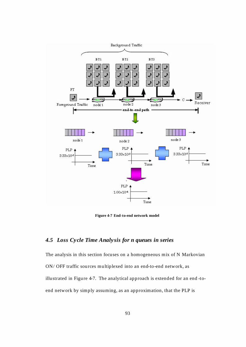
93
Figure 4-7 End-to-end network model
4.5 Loss Cycle Time Analysis for n queues in series
The analysis in this section focuses on a homogeneous mix of N Markovian
ON/OFF traffic sources multiplexed into an end-to-end network, as
illustrated in Figure 4-7. The analytical approach is extended for an end-to-
end network by simply assuming, as an approximation, that the PLP is
94
divided equally among all the queues in series (with same link rates). So
IPLP = TPLP/n, and therefore
( )2
2
.
..
p
oncycle
ACTPLP
nThT
−= Equation
4-20
In this case, the mean time until the probe is lost for an end-to-end network
is given by:
cyclemt T.γµ = = ( )
−
−−
−−
on
pp
Th
TAC
p
on
p
eAC
ThT
.
.
1.1
1
1 . ( )2
2
.
..
p
on
ACTPLP
nTh
− Equation
4-21
4.6 Numerical Examples using the analysis
This section applies the previous analysis and investigates the mean time
taken for the probes to encounter an overflow period across buffered access
links and across ‘n’ queues (where n=3) with the same link rates throughout,
using numerical examples. The standard VoIP model was used with the
following parameter values to generate all the numerical results:
• VoIP traffic sources: Ton = 0.96 seconds, Toff = 1.69 seconds, ON rate of
the codec, h = 64kbps (170 packets/sec)
• Packet size = 47 bytes
• Buffer output rate is set for low rate access speeds, i.e. 512 kbps or
2Mbps

95
• PLP = 10-4
• Load is varied about the key operating point of 80% [16] [26]
• Buffer size is adjusted to keep the PLP at 10-4 (to maintain the target
PLP as the load increases the buffer length is re-calculated and
adjusted accordingly)
• Number of VoIP sources multiplexed is adjusted to set the load to the
desired value
The VoIP specific parameter settings are widely used as representative of
VoIP traffic sources [50] [74], and particularly the behaviour of G.711 (PCM)
which is a high-bit-rate ITU standard codec, operating at 64 kbps.
Recommendation Y.1541 [48], (already discussed in chapter 3) specifies a
PLP of less than 10-3, and so in all the following numerical results a target a
PLP of 10-4 has been used [48] [49] [50].
To maintain a target PLP of 10-4, an increase in the traffic load requires an
increase in the buffer length. This is due to the fact that for the purposes of
fair comparison, the service rate, which represents the link bandwidth, has
to be kept constant. There is known to be a log-linear relationship between
the PLP and the buffer length, x as shown in Equation 4-22. The full
derivation of Equation 4-22 is in Appendix B. Equation 4-22 has been used

96
for the calculation of the buffer length for the VoIP based simulation
experiments reported in this section:
1
.. +
−=
x
p sa
ACDh
PLP [44] Equation 4-22
Table 4-1 shows the buffer length and the number of sources for the varying
loads (˜60%-90%) for both buffered access links and end-to-end networks.
Table 4-1 Calculation of the buffer length for single access and end-to-end networks
Figure 4-8 shows the results for both a single access and an end-to-end
scenario over different link rates, and over load values ranging from
between 0.5 and 0.9. It can be seen from the results in Figure 4-8 that the
time required for a probe to be lost (due to encountering an overflowing
buffer) can be very large. Even the VoIP traffic, smooth by Internet
standards, is actually significantly bursty when buffered over a low rate
access link (e.g. 256-512 kbps).

97
Ton=0.96s, Toff=1.69s, PLP=1E-4, h=64kbpsANALYSIS
1.E-02
1.E-01
1.E+00
1.E+01
1.E+02
1.E+03
0.6 0.7 0.8 0.9
Load
256K: single access
256K: end-to-end
512K: single access
512K: end-to-end
2M: single access
2M: end-to-end
Figure 4-8 Time for the probes to encounter an overflowing buffer
For the higher link rates (e.g. 2M), tµ is significantly lower than the lower
link rates (e.g. 512K). The length of the buffer required for a 2M link to
achieve a PLP of 10-4 is smaller because of its higher service rate and hence
the time taken for a probe to encounter an overflow also reduces.
Figure 4-9 Effect of different probe rates
Tim
e fo
r pr
obes
to s
ee
an o
verf
low
(in
hour
s)
98
In Figure 4-9 the mean time required by the probes to encounter an overflow
is plotted against time and the effect observed for different probe rates. The
expected time for a probe to encounter an overflow decreases because the
value of Tp has been increased. As the streams of probes are coming more
frequently than before, it thereby decrea ses the time taken for a probe to see
an overflow. However, simply increasing the probe rate may introduce large
measurement inaccuracies due to the additional load imposed by the probe
packets [32].
4.7 Summary
In this chapter, an analysis for the mean time for a probe to encounter an
overflowing buffer was presented. However, this analysis is limited because
it finds the mean time until a probe first sees an overflowing buffer. This
does not use any measure of the variance of the overflow process. The next
chapter develops an enhanced form of analysis using, the variance of the
number of packets between lost packets, and shows how this can be applied
to find the number of samples required to measure the PLP within a given
level of required accuracy.
99
5 Sampling Theoretic Bounds on the Accuracy of Probing
Extending the work of chapter 4, this chapter develops bounds, based on
Sampling Theory [152] [153], on the accuracy of PLP measurements. This
analytical approach accounts for the inherent burstiness of the buffer
overflow process, and hence the packet loss events. This approach allows the
prediction of the number of samples, and hence time required, to accurately
measure the PLP across a network path, within a predefined measurement
error.
5.1 Variability of the distribution of the number of packets
between lost packets for a buffered link
The analysis focuses on the effect of overflowing buffers on the loss of
packets, and in particular the variance of the inter-packet loss distribution
since the reciprocal of the number of not lost packets between lost packets
gives the PLP. The expected number of packets lost per overflow period in
Equation 4-7 derived in chapter 4 is also used in this analysis.
( )2
2 ..
p
ponp
AC
ATh
−=µ Equation
5-1
During buffer overflow periods the time between packet losses is
approximately:

100
(Ron – C)-1 =
− p
p
AC
Ah. -1 Equation
5-2
Such a high loss rate to service rate ratio is indicative that, during the
overflow periods, packets will be lost virtually consecutively. A more
substantial evaluation of this is given in Table 5-1 where for e.g. 50% load,
170 packets are lost with a mean of 3.23 x 101 numbers of not lost packets
between the lost packets during the overflow period. This small value of the
inter-loss period indicates that packets are lost almost consecutively.
Load Ron (packet/sec) C (packet/sec) (Ron - C) 1/ (Ron -
C) Mean number of not lost packets
between lost packets
0.1 5338 5319 18.88 5.30E-02 2.83E+02 0.2 5362 5319 42.5 2.35E-02 1.26E+02 0.3 5392 5319 72.86 1.37E-02 7.39E+01 0.4 5433 5319 113.3 8.83E-03 4.80E+01 0.5 5489 5319 170 5.88E-03 3.23E+01 0.6 5574 5319 255 3.92E-03 2.19E+01 0.7 5716 5319 396 2.53E-03 1.45E+01 0.8 5999 5319 680 1.47E-03 8.82E+00 0.9 6849 5319 1530 6.54E-04 4.48E+00
Table 5-1 Calculation of the number of not lost packets between losses
However, during the non-overflow part of the cycle, the time and the
number of not-lost packets between lost packets will be much larger, and
much more randomly distributed, as illustrated in Figure 5-1. During non-
overflow periods there are no packet losses, and these periods provide the
major contribution to the variance of the distribution of the number of not-
lost packets between lost packets.
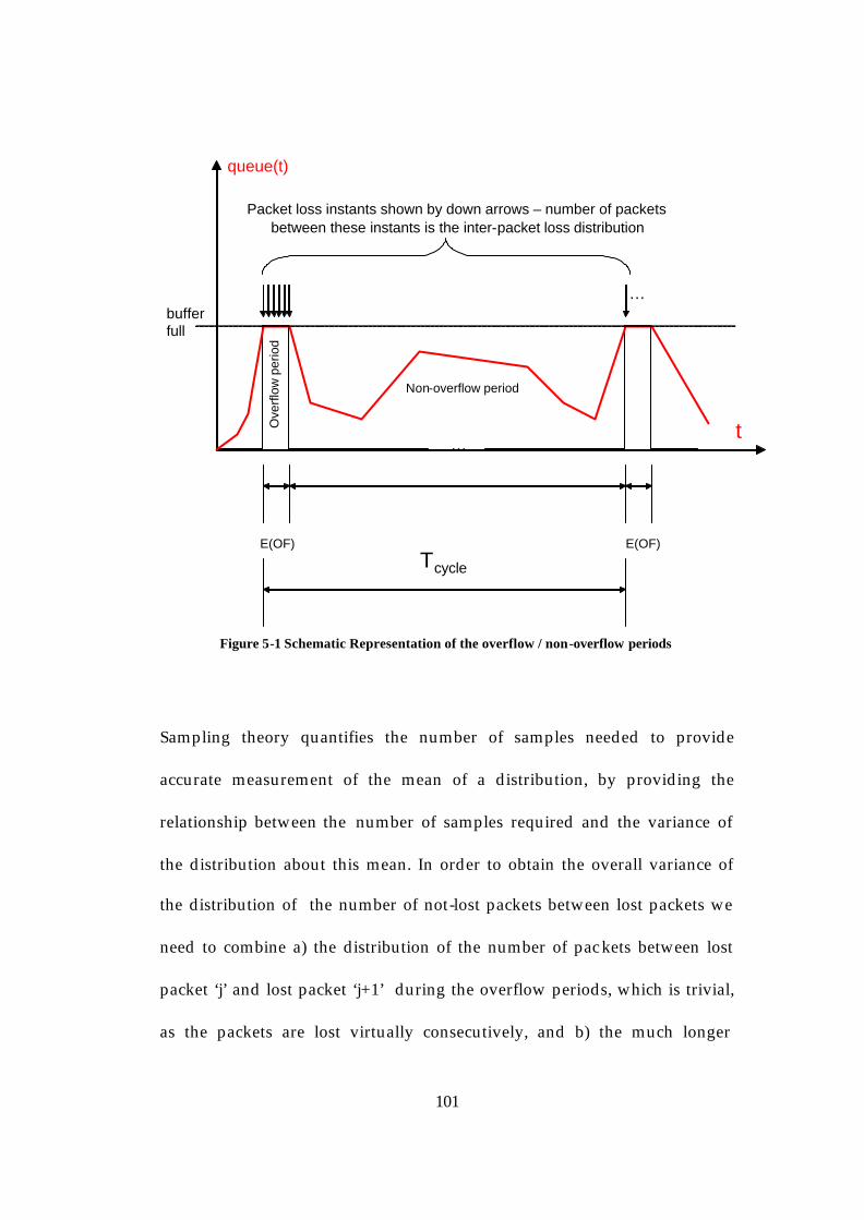
101
…
E(OF) E(OF)
Tcycle
…
Packet loss instants shown by down arrows – number of packets between these instants is the inter-packet loss distribution
Ove
rflo
w p
erio
d
Non-overflow period
queue(t)
t
buffer full
Figure 5-1 Schematic Representation of the overflow / non-overflow periods
Sampling theory quantifies the number of samples needed to provide
accurate measurement of the mean of a distribution, by providing the
relationship between the number of samples required and the variance of
the distribution about this mean. In order to obtain the overall variance of
the distribution of the number of not-lost packets between lost packets we
need to combine a) the distribution of the number of packets between lost
packet ‘j’ and lost packet ‘j+1’ during the overflow periods, which is trivial,
as the packets are lost virtually consecutively, and b) the much longer

102
“random” period between lost packet ‘j’ and lost packet ‘j+1’ when ‘j’ is the
last packet lost in an overflow period, and so the ‘j+1’th loss occurs after the
next non-overflow period.
To find the overall variance of the distribution of the number of packets
between losses, we can combine the overflow and non-overflow periods
through their 2nd moments, as done previously in [19] [50]. Using Y to
denote the R.V. representing the number of (not-lost) packets between lost
packet ‘j’ and lost packet ‘j+1’ E[Y] can be defined as:
E[Y] = the mean number of not -lost packets between lost packets (= PLP-1)
NOF = mean number of not-lost packets between consecutive lost packets
during overflow periods
NNOF = mean number of packets in non-overflow periods (i.e. the number of
not-lost packets when ‘j+1’ is the first lost packet in a new overflow
period)
q = Prob(an inter-packet-loss period is contained within an overflow period)
This is because, on average, 1−pµ out of pµ inter-loss-periods are contained
within the overflow period (the last of the pµ is the non-overflow period) so
(Figure 5 -2):

103
p
pqµ
µ 1−= Equation
5-3
Figure 5-2 Schematic representation of “ q”
( ) NOFOF NqNqYE .1.][ −+= Equation 5-4
where 0≈OFN as the packets are lost virtually consecutively in the overflow
period. A numerical evaluation of this was shown in Table 5-1.
As already used in chapter 4, an accurate model is that non -overflow periods
are approximated by a geometrically distributed number of packets. For any
geometric distribution:
Mean of the Geometric distribution = p1 Equation
5-5
Variance of the Geometric Distribution = 2
1p
p− Equation 5-6

104
Mean square for the Geometric Distribution 2
2
2
211p
ppp
p −=
+
−
Equation 5-7
where ‘p’ is the parameter of the Geometric distribution.
In this chapter, p is found from the overall mean number of packets between
lost packet ‘j’ and lost packet ‘j+1’. This overall mean is the reciprocal of the
PLP, but it may also be constructed from the conditional means, during the
overflow period, POF, and during the non-overflow period, PNOF:
For the first 1−pµ out of pµ inter-loss-periods:
OF
OF Np
1= Equation
5-8
and for the last of the µp inter-loss-periods:
NOF
NOF Np
1= Equation
5-9

105
Using the average number of packets lost in an overflow period the
conditional expectations are defined as:
EOF[Y2] = mean square number of packets between lost packets given we are
considering the first 1−pµ out of pµ lost packets , i.e. those lost in
the overflow period.
ENOF[Y2] = mean square number of packets between lost packets given we
are considering the last one of the pµ lost packets, i.e. the one
followed by the non-overflow period.
As already noted, the loss rate is extremely high during overflow periods, so
during overflow periods packets are being lost virtually consecutively, and
with a virtually fixed time between losses (i.e. virtually constant loss rate):
EOF[Y2] ˜ 0
Thus, when considering the number of lost packets between the final lost
packet in the overflow period, and the next lost packet, by definition at the
start of the next overflow period, it was observed that:
2
2
22 211][
pp
ppp
YENOF
−=
+
−= = ( )
−
NOFNOF NN 12.2 Equation
5-10
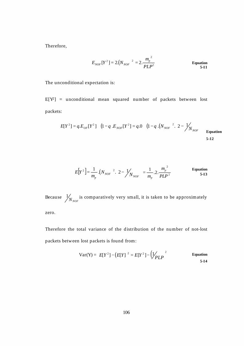
106
Therefore,
( )2
222 .2.2][
PLPNYE p
NOFNOF
µ== Equation
5-11
The unconditional expectation is:
E[Y2] = unconditional mean squared number of packets between lost
packets:
( ) ( ) ( )
−−+=−+=
NOFNOFNOFOF NNqqYEqYEqYE 12..10.][.1][.][ 2222
Equation
5-12
[ ]p
YEµ12 = ( )
−
NOFNOF NN 12.. 2
2
2
.2.1
PLPp
p
µ
µ=
Equation 5-13
Because NOFN
1 is comparatively very small, it is taken to be approximately
zero.
Therefore the total variance of the distribution of the number of not-lost
packets between lost packets is found from:
Var(Y) = ( ) ( )2222 1][][][ PLPYEYEYE −=− Equation
5-14

107
Therefore Equation 5-15 gives the expression for the unconditional Variance
of the distribution of the number of packets between successive packet
losses:
( ) =YVar ( ) 222
2
22
1
.
...21.2
PLPPLPAC
ATh
PLPPLP p
ponp −−
=−µ
( )
−
−= 1
...212
2
2p
pon
AC
ATh
PLP Equation
5-15
To investigate how many samples of the distribution (of packets between
loss packets) would be needed to achieve the required level of accuracy
using sampling theory, define:
N = the number of measurements required
tN-1, 1-α/2 = the Student t-distribution value for N-1 degrees of freedom (i.e.
sample size = N), and (100-a)% confidence interval for the
estimate of the mean number of lost packets between lost packet ‘j’
and lost packet ‘j+1’
δ = the chosen value of absolute error in the measurements
SN = standard deviation of the distribution
S2N = variance of the distribution
For the measured (sampled) mean to be within the error ±δ of the true
mean, N must be such that:
NS
t 2
2N
21,1N
≤
δ⋅α
−−
2
Equation
5-16
108
Since, ( )YVarSN =2 , (5-15) and (5-16) can be used to discover how many
samples would be needed to measure the packet loss probability with a
given absolute measurement error.
5.2 Measuring an end-to-end path across a realistic network Figure 5-3 shows a generic model for a typical end-to-end networking
scenario consisting of the heavily loaded edge routers being connected via
their respective local access networks and the lightly loaded core routers.
The edge router is likely to be around 2Mbps while the backbone network is
likely to have link rates at 16STM.

109
Figure 5-3 A generic model for an end-to-end network scenario
Figure 5-4 depicts a slightly thinned-out version of a typical end-to-end
network. It has been thinned to remove most of the link replication (this
replication exists purely to offset the effects of link failure and thereby to
provide “5 9’s” level of availability).
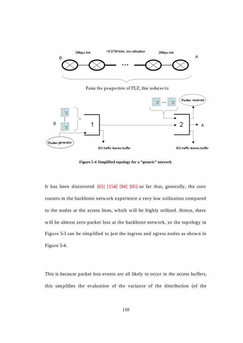
110
Figure 5-4 Simplified topology for a “generic” network
It has been discovered [65] [154] [84] [85] so far that, generally, the core
routers in the backbone network experience a very low utilization compared
to the nodes at the access lines, which will be highly utilized. Hence, there
will be almost zero packet loss at the backbone network, so the topology in
Figure 5-3 can be simplified to just the ingress and egress nodes as shown in
Figure 5-4.
This is because packet loss events are all likely to occur in the access buffers,
this simplifies the evaluation of the variance of the distribution (of the

111
number of packets between lost packets) by limiting the number of link-
buffer pairs that need be considered. Variances across independent links will
roughly be additive, so the total variance for a path can be evaluated by
applying Equation 5-15 to each path and summing to give the total.
( ) =YVar ee2( )YVar
N
nn∑
=1 Equation
5-17
where n is the number of queues.
and from Equation 5-17 the number of samples of the distribution is:
ee
N
NNn
St 22
22
21,1
.. ≤
−− δα
Equation
5-18
5.3 Numerical Examples
The purpose of this section is twofold: 1) validation of Equation 5-15 and 2)
to investigate the likely number of samples needed for a single buffered
access link.
5.3.1 Measurement (Simulation) Time
A simulation is said to be in steady state, not when the performance
measurements become constant but when the distribution of the
measurements becomes (close to being) invariant with time. In order to
measure the PLP, it is important for the system to reach steady state to be
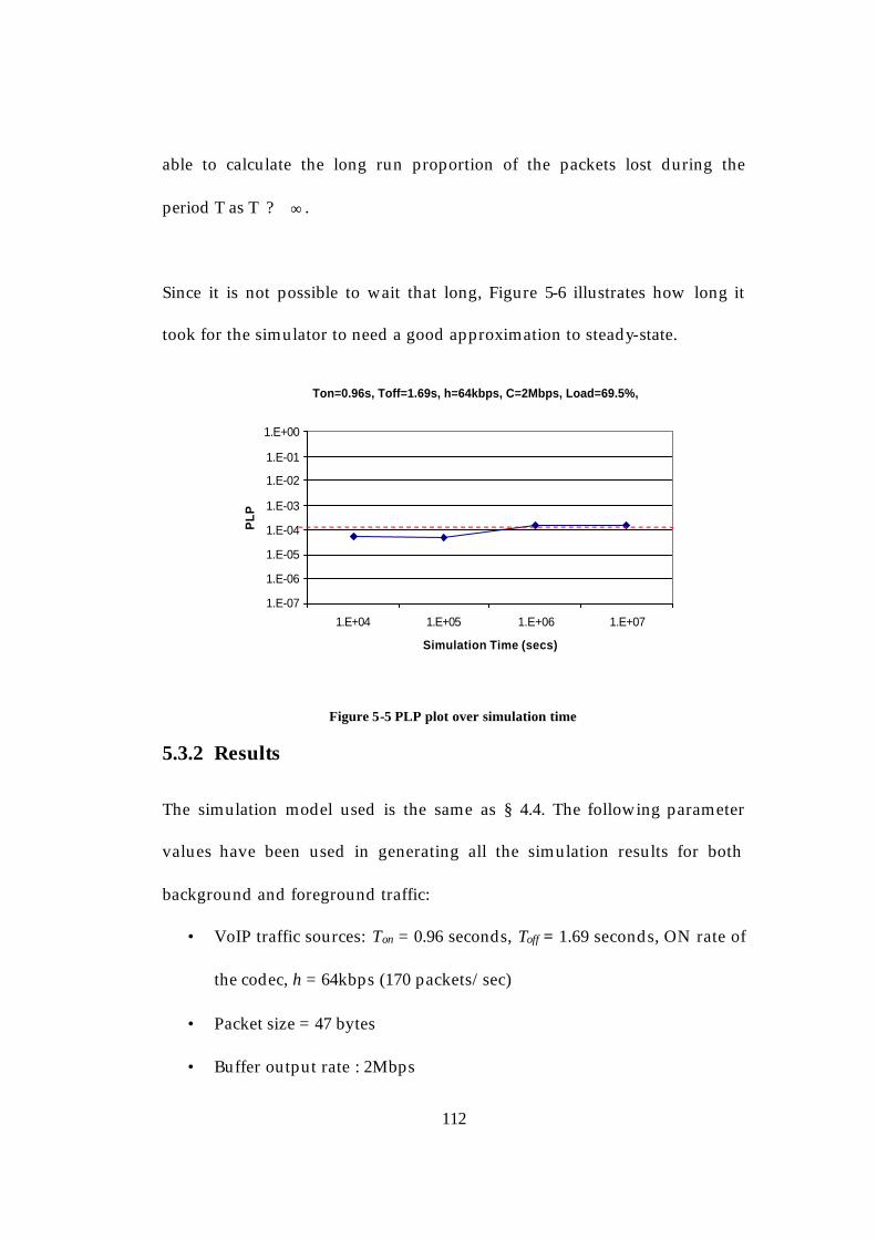
112
able to calculate the long run proportion of the packets lost during the
period T as T ? ∞ .
Since it is not possible to wait that long, Figure 5-6 illustrates how long it
took for the simulator to need a good approximation to steady-state.
Figure 5-5 PLP plot over simulation time
5.3.2 Results
The simulation model used is the same as § 4.4. The following parameter
values have been used in generating all the simulation results for both
background and foreground traffic:
• VoIP traffic sources: Ton = 0.96 seconds, Toff = 1.69 seconds, ON rate of
the codec, h = 64kbps (170 packets/sec)
• Packet size = 47 bytes
• Buffer output rate : 2Mbps
Ton=0.96s, Toff=1.69s, h=64kbps, C=2Mbps, Load=69.5%,
1.E-07
1.E-06
1.E-05
1.E-04
1.E-03
1.E-02
1.E-01
1.E+00
1.E+04 1.E+05 1.E+06 1.E+07
Simulation Time (secs)
PL
P

113
• PLP = 10-4
• Load is varied about the key operating point of 80%
• Buffer size is adjusted to keep the PLP at 10-4 (to maintain the target
PLP as the load increases the buffer length is re-calculated and
adjusted accordingly)
• Number of VoIP sources multiplexed is adjusted to set the load to the
desired value
The simulation results are concerned with the upper end of the potential
range of busy hours’ utilisation values for a single access link. The load is set
by adjusting the number of VoIP sources, and then the buffer length set
appropriate to the desired loss probability using Equation 4-22 from § 4.6.
Tables 5-2 and 5-3 compare the analysis with simulation, for ingress/egress
link speed of 2Mbps. It can be seen that there is good agreement between the
analysis and the simulation results to give confidence that the analysis is
broadly accurate enough to provide an engineering estimate of the Variance
and hence the number of samples required.
Load Variance by simulation
Variance by analysis
0.695 7.76E+09 7.69E+09 0.799 2.82E+10 2.05E+10 0.845 6.17E+10 3.67E+10 0.879 1.02E+11 1.04E+15
Table 5-2 Comparing variance for a single buffer by simulation and analysis

114
Table 5-3 Comparing variance for an end-to-end network by simulation and analysis
Table 5-3 shows the variance of the number of not-lost packets between
losses for an end-to-end network. It can be seen that the value of Var(Y) is
shown to be two times for an end-to-end network when compared to a
single access buffer. This agrees with intuition, as the variance for an end-to-
end network must be greater than the individual variances for single
buffered links.
It can be observed from Figure 5-6 and Figure 5-7 that as the load increases,
the length of the non-overflow period becomes longer as the queue becomes
more variable due to the increase in the buffer length.
Load Variance by simulation
Variance by analysis
0.695 3.07E+10 3.00E+10 0.799 1.26E+11 8.21E+10 0.845 3.80E+12 1.46E+11 0.998 1.02E+16 1.04E+15

115
Figure 5-6 Schematic representation of the overflow periods for a load of 65%
Figure 5-7 Schematic representation of the overflow periods for a load of 85%

116
1.E+00
1.E+01
1.E+02
1.E+03
1.E+04
1.E+05
1.E+06
0.695 0.799 0.845 0.879
Load
Nu
mb
er o
f s
amp
les
req
uir
ed
for 10% error end to end
for 50% error end to end
for 100% error end to end
for 10% error single access
for 50% error single access
for 100% error single access
Figure 5-8 Comparing the number of samples required single buffer and end-to-end network
Figure 5-8 shows the number of samples required for the variance of the
number of not lost packets between the lost packets. From these figures it
can be observed that:
• The analysis provides a simple and effective means of accurately
estimating the variance of the number of packets between losses for
all higher levels of load.
• The number of samples increases with increasing load and as
sampling theory states that the greater the variability of the sampled
data, the more samples are needed for accurate estimation as the load
increases.

117
5.3.3 Effect on the Probes and on the Number of Busy Hours
Required for Sampling
When probing, on average every 10,000th (for PLP=10-4) probe provides a
sample of the distribution of the number of not lost probes between lost
probes. Thus, for a PLP of 10-4 as only 1 probe in 10,000 ‘samples’ of the
distribution will be lost on average, it means that for every N samples,
N*10,000 probes will be required.
The effect of this can be observed in Table 5-4 for a link rate of 2M, where
for a load value of 80%, an excessive number of probes (̃ 10,000*1400 =
14M) will be required even to evaluate the PLP with an accuracy of 100%
error over a single link only. 14M probes will take approximately 4000 busy
hours at the SAA default rate of one probe per second, which is clearly too
long.
Table 5-4 Number of busy hours required by the probes for a PLP of 10-4

118
Table 5-5 Number of busy hours required by the probes for a PLP of 10-4
Table 5-6 Number of busy hours required by the probes for a PLP of 10-4
Two possible solutions to the problem of excessive sampling are:
i) Increase the probing rate: to reduce the number of
busy hours required (for probing) down by a factor
of 100 would require an increase in the probing rate
by the same factor, which is not practical.

119
ii) Reduce the specified level of accuracy: a 100% error
actually corresponds to an estimate which is within
the bound of 5e-5 < PLP < 2e-4, which is actually
quite tight for a sampled measure. Therefore, for a
PLP of 2e-4, it will take about 900 busy hours which
is too long unless the probing rate is also increased
10 times.
Table 5-7 shows that an increased PLP (to 10-3) and the same load value and
link rate will require about 4 busy hours with an accuracy of 100% error for a
single link.
Table 5-7 Number of busy hours required by the probes for a PLP of 10-3

120
Table 5-8 Number of busy hours required by the probes for a PLP of 10-3
Table 5-9 Number of busy hours required by the probes for a PLP of 10-3
Figure 5-9 depicts the number of busy hours required by the probes for a
PLP of 10-4 with different link rates.
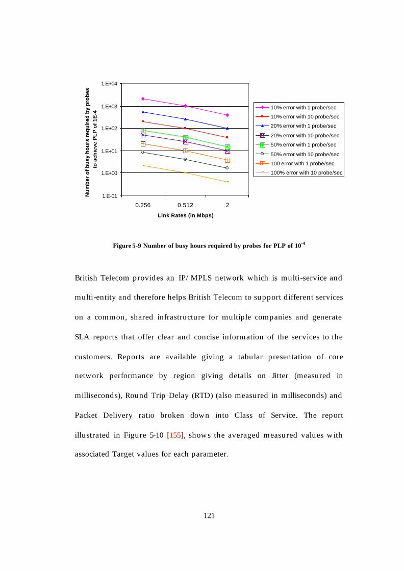
121
1.E-01
1.E+00
1.E+01
1.E+02
1.E+03
1.E+04
0.256 0.512 2
Link Rates (in Mbps)
Nu
mb
er o
f b
usy
ho
urs
req
uir
ed b
y p
rob
es
to a
chie
ve P
LP
of
1E-4
10% error with 1 probe/sec
10% error with 10 probe/sec
20% error with 1 probe/sec
20% error with 10 probe/sec
50% error with 1 probe/sec
50% error with 10 probe/sec
100 error with 1 probe/sec
100% error with 10 probe/sec
Figure 5-9 Number of busy hours required by probes for PLP of 10-4
British Telecom provides an IP/MPLS network which is multi-service and
multi-entity and therefore helps British Telecom to support different services
on a common, shared infrastructure for multiple companies and generate
SLA reports that offer clear and concise information of the services to the
customers. Reports are available giving a tabular presentation of core
network performance by region giving details on Jitter (measured in
milliseconds), Round Trip Delay (RTD) (also measured in milliseconds) and
Packet Delivery ratio broken down into Class of Service. The report
illustrated in Figure 5-10 [155], shows the averaged measured values with
associated Target values for each parameter.

122
94.79% Packet Delivery Ratio
Figure 5-10 BT MPLS Weekly Customer Network Performance Summary Report
It can be seen from Figure 5-10 that the average Packet Delivery Ratio is
94.79% from Core-AM-AM-COS1 with a PLP of approximately 5x10⁻², which
is still quite high for real-time applications like VoIP [74] [142] [143] [144]
[145] [146].
5.4 Summary
This chapter develops sampling bounds for probing PLP across single
buffered links and end-to-end networks. The variance of the inter-packet

123
loss distribution for the single access was lower than the end-to-end
networks. It also showed the effect of the probes on the number of busy
hours and concluded that increasing the PLP to 10-3 made measurement
easier compared to the target PLP of 10-4. This chapter studied VoIP traffic,
which is not very bursty. Thus, much burstier “data” traffic could give rise
to significantly larger variances; hence chapter 6 applies the analysis to
“data” traffic.

124
6 Measuring Power Law Traffic using Active Probing This chapter discusses the concept of self similarity, its impact and contrast
with Markovian traffic, including highlighting the background to self-
similarity in networks and related issues in the context of traffic
measurement. Numerical results obtained from simulations are presented,
and they show how difficult it can be to measure loss performance
accurately in the presence of Power Law traffic.
6.1 Self-Similarity and Long Range Dependence The Markovian traffic models discussed in § 3.3.1 have been widely used for
traffic modeling in the past few decades [44] [113] [114]. With the
convergence of voice and data, the traditional Markovian models may be
inadequate to capture the behaviour of the future multi-service network [2]
as the Markovian model creates traffic that is bursty over fine time scale but
smooth over large timescale. Thus, new traffic models have been developed
[121] using self-similar process [121], such that the network performance can
be accurately predicted, and eventually, service delivered with the expected
quality. This self-similar process is in stark contrast to the traditional
Markovian traffic, in the sense that the traffic burstiness remains the same
regardless the degree of resolution [121] [113].
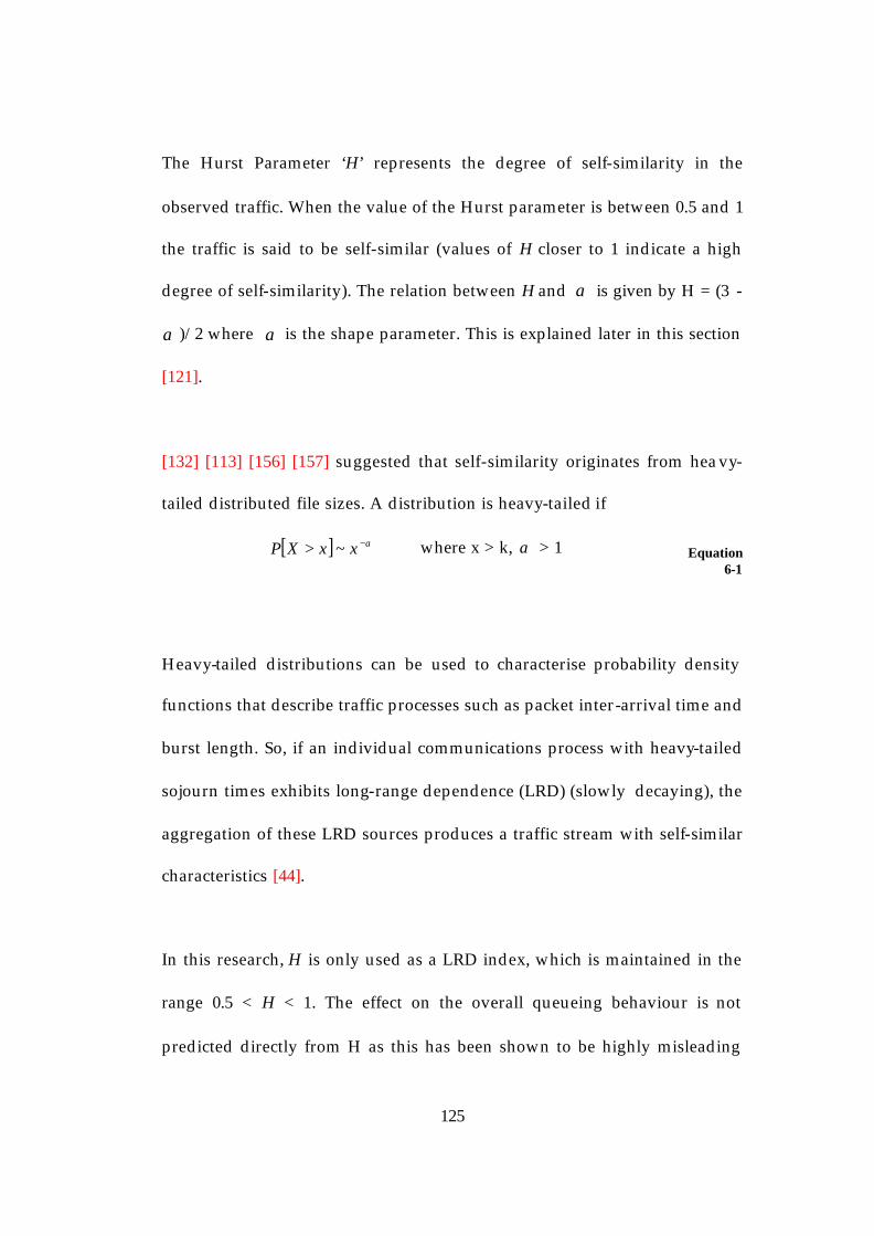
125
The Hurst Parameter ‘H’ represents the degree of self-similarity in the
observed traffic. When the value of the Hurst parameter is between 0.5 and 1
the traffic is said to be self-similar (values of H closer to 1 indicate a high
degree of self-similarity). The relation between H and α is given by H = (3 -
α )/2 where α is the shape parameter. This is explained later in this section
[121].
[132] [113] [156] [157] suggested that self-similarity originates from heavy-
tailed distributed file sizes. A distribution is heavy-tailed if
[ ] α−> xxXP ~ where x > k, α > 1 Equation 6-1
Heavy-tailed distributions can be used to characterise probability density
functions that describe traffic processes such as packet inter-arrival time and
burst length. So, if an individual communications process with heavy-tailed
sojourn times exhibits long-range dependence (LRD) (slowly decaying), the
aggregation of these LRD sources produces a traffic stream with self-similar
characteristics [44].
In this research, H is only used as a LRD index, which is maintained in the
range 0.5 < H < 1. The effect on the overall queueing behaviour is not
predicted directly from H as this has been shown to be highly misleading

126
and potentially incorrect [158] [164]. In fact, studies in [159] [160] have
discovered that the characteristics of the On period and often more
important than H for teletraffic engineering in terms of overall queueing
behaviour. This is important as the work reported in this thesis is focused on
the impact of the On period on the overall PLP.
The Pareto distribution (or Power Law distribution) is the simplest form of a
heavy-tailed distribution. This distribution can have high or even infinite
variance and possibly infinite mean also. It has been used in this thesis
because of its simplicity and its widely accepted [44] [156] [119]. Its
probability distribution and density function are given by:
( )α
−=
xkxF 1 where x > k, α > 1 Equation
6-2
( )1
.+
=
ααxk
kxf where x > k, α > 1
Equation 6-3
where ‘k’ is the scaling parameter which defines the minimum value that
the distribution can accommodate, and α is the shape parameter which
determines the characteristic ‘decay’ of the distribution. If 2≤α , the
distribution has infinite variance. As α decreases, a larger proportion of the
generated random variables lie in the tail of the distribution. The
distribution has a mean equal to

127
( ) kxE .1
−=
αα Equation
6-4
It should be noted that for Equation 6-4 to be correct α > 1 otherwise the
Pareto distribution has an infinite mean.
Figure 6-1 gives a simple pictorial comparison between Pareto and
exponential distribution. There is a significant difference between the ways
in which their probability masses are located. The exponential distribution
has the logarithm of the probability decaying linearly as x increases while
the Pareto distribution falls gradually with a large portion of random
variables in the tail. For that reason, the possibility of getting extremely large
values cannot be ignored when the traffic models use the Pareto distribution.
Figure 6-1 Comparison of Exponential and Pareto Distributions
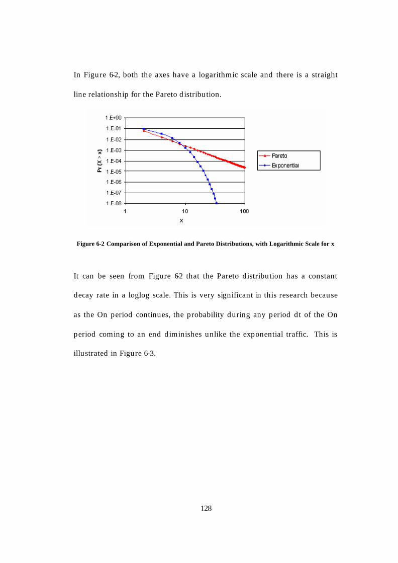
128
In Figure 6-2, both the axes have a logarithmic scale and there is a straight
line relationship for the Pareto distribution.
Figure 6-2 Comparison of Exponential and Pareto Distributions, with Logarithmic Scale for x
It can be seen from Figure 6-2 that the Pareto distribution has a constant
decay rate in a loglog scale. This is very significant in this research because
as the On period continues, the probability during any period dt of the On
period coming to an end diminishes unlike the exponential traffic. This is
illustrated in Figure 6-3.

129
Figure 6-3 Comparison of Exponential and Power-law On times
6.2 Simulation Model
For the purpose of fair comparison, the On/Off model chosen is the same as
for Markovian (chapter 5), but with Pareto distributed On times [161]. Figure
6-4 depicts the simulation model used which is implemented using Network
Simulator 2 (NS2). The code for NS2’s Pareto On/Off source is modified
such that the Off period uses an exponential distribution and is renamed as
ExPareto. The On period is unaltered (i.e. left as Pareto distributed). The

130
Geo/Pareto/1 can be used for the verification of the ExPareto model. This is
discussed in § 6.2.1.
Figure 6-4 ExPareto On/Off Model
6.2.1 Verification of ExPareto traffic source (using
Geo/Pareto/1)
The Geo/Pareto model can be used as a verification of the ExPareto model
because the number of packets in a batch for the Geo/Pareto/1 is discrete
version of the Pareto distribution and the number of time slots between the
batches is Geometrically distributed [44]. This is analogous with the
continuous Pareto distributed On times and exponentially distributed Off
times for the ExPareto model. This is illustrated in Figure 6 -5.
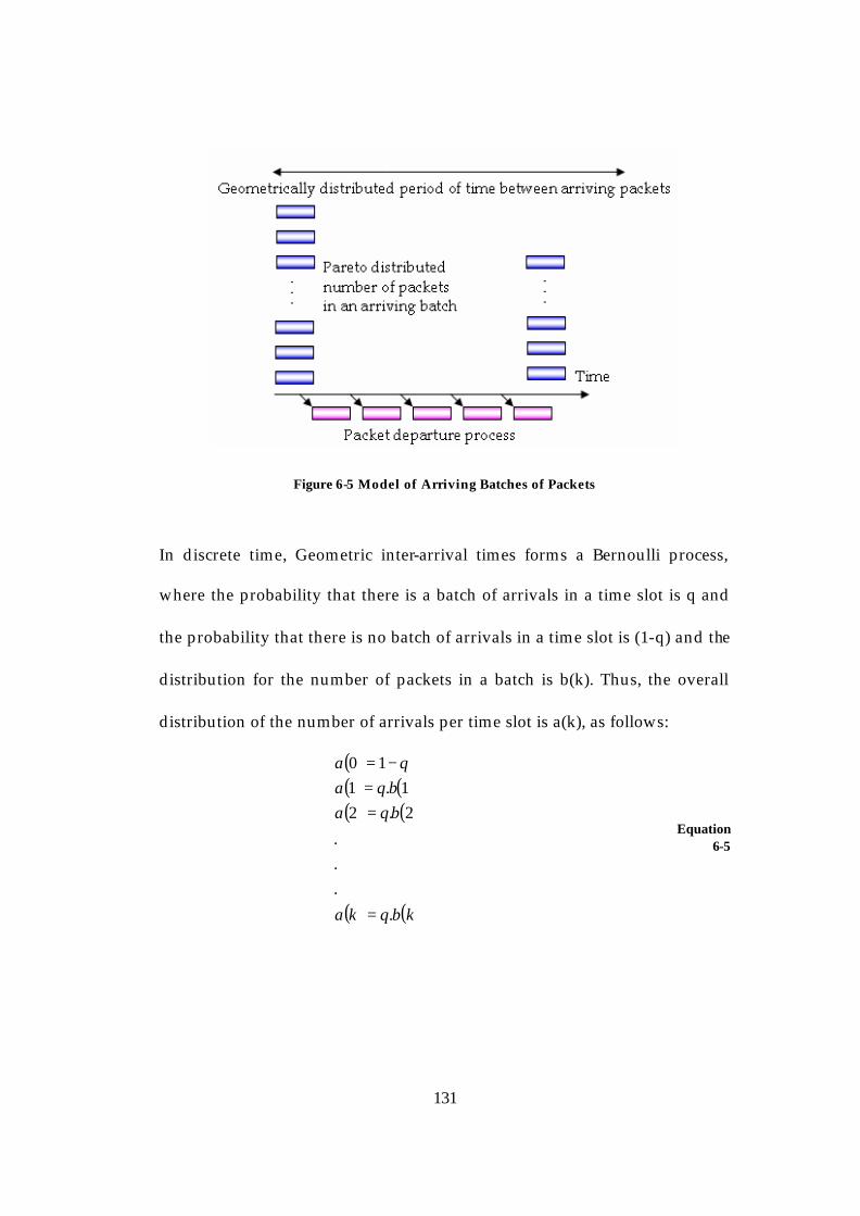
131
Figure 6-5 Model of Arriving Batches of Packets
In discrete time, Geometric inter-arrival times forms a Bernoulli process,
where the probability that there is a batch of arrivals in a time slot is q and
the probability that there is no batch of arrivals in a time slot is (1-q) and the
distribution for the number of packets in a batch is b(k). Thus, the overall
distribution of the number of arrivals per time slot is a(k), as follows:
( )( ) ( )( ) ( )
( ) ( )kbqka
bqabqa
qa
.
.
.
.
2.21.1
10
=
==
−=
Equation 6-5

132
where q (Equation 6-6) is derived from the load, ρ and the shape parameter,
α
1−
==α
αρρ
Bq Equation
6-6
and b(k) (Equation 6-7) is derived from a discrete version of the Pareto
distribution by taking the interval [k-0.5, k+0.5] on the continuous Pareto
distribution from Equation 6-2 [44].
( ) ( ) ( )αα
+−
−=+−−=
5.01
5.01
5.05.0kk
xFxFkb Equation
6-7
So, b(k) is the conditional probability distribution for the number of packets
arriving in a time slot, given that there is a batch and a(k) is the
unconditional probability distribution for the number of packets arriving in
a time slot, whether there is an arriving batch or not.
For this queueing model, s(k), or the probability there are k in the system at
the end of any time unit is given as:
s(k) = )0(
)().()1().0()1(1
1
a
ikaiskasksk
i∑
−
=
−−−−− Equation
6-8
The derivation of this is in Appendix C.
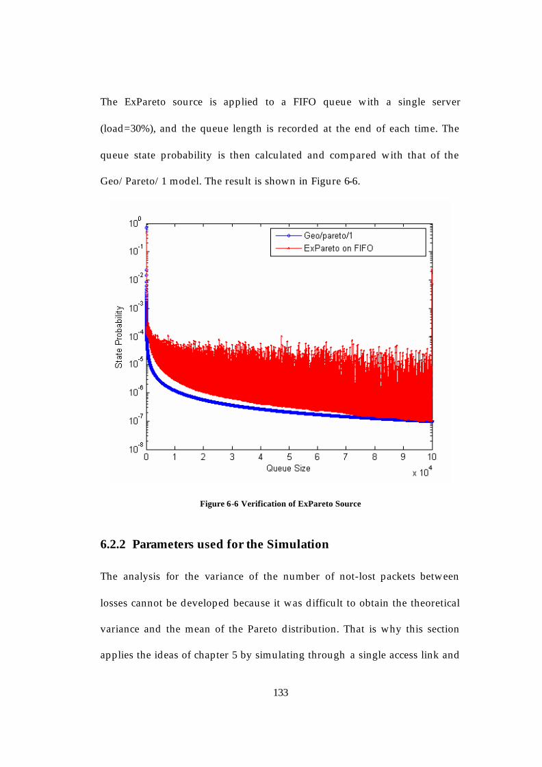
133
The ExPareto source is applied to a FIFO queue with a single server
(load=30%), and the queue length is recorded at the end of each time. The
queue state probability is then calculated and compared with that of the
Geo/Pareto/1 model. The result is shown in Figure 6-6.
Figure 6-6 Verification of ExPareto Source
6.2.2 Parameters used for the Simulation
The analysis for the variance of the number of not-lost packets between
losses cannot be developed because it was difficult to obtain the theoretical
variance and the mean of the Pareto distribution. That is why this section
applies the ideas of chapter 5 by simulating through a single access link and

134
further investigating the variance of the inter-packet loss distribution from
the simulation results. The Pareto model used is 10 times as bursty as the
Markovian model in chapter 5 and the following parameter values are used
to generate all the simulation results:
• Traffic sources: Ton = 9.6 seconds, h = 2Mbps (250 packets/sec)
• Packet size = 1000 bytes
• PLP = 10-4
• Buffer size is adjusted to keep the PLP at 10-4 (to maintain the target
PLP as the load increases the buffer length is re-calculated and
adjusted accordingly)
• Number of data sources multiplexed is set at a constant value of 50
• Toff is adjusted accordingly to set the load
h is used equal to the link rate as [162] and N was used as 50 because lower
number of sources gave very low loads.
6.3 Buffer Length Analysis and its Limitations The buffer length as in chapter 5 has to be adjusted accordingly in order to
maintain the desired PLP. There is a relationship between the PLP and the
buffer length, x as shown in Equation 6-9 [163]. The full derivation of
Equation 6-9 is given in Appendix D:
PLP = ρ.X[log2(1 – (1/ρ - 1)(exp(((C-Ap)2)/(Ton.h2.C)) - 1))
Equation
6-9

135
Table 6-1 shows the buffer length, and Toff for the varying loads for buffered
access link calculated from Equation 6-3 and Figure 6-7 depicts the buffer
length with varying loads for Ton=9.6sec, h = 2M,C=2M and N = 50.
Load Buffer length Toff 0.1 0.6841 4790 0.2 1.4611 2390 0.3 17.071 1590 0.4 1.29E+03 1190
0.592 8.74E+08 800 0.676 4.84E+13 700 0.787 5.60E+25 600 0.941 1.06E+118 500
Table 6-1 Calculation of the buffer length
1.E-101.E+001.E+101.E+201.E+301.E+401.E+501.E+601.E+701.E+801.E+90
1.E+1001.E+1101.E+120
0.1 0.2 0.3 0.4 0.592 0.676 0.787 0.941
Load
Buf
fer
Leng
th
ExPareto
Figure 6-7 Relationship between the load and the buffer length using Equation 6-3
Equation 6-9 was compared with the simulation results and the results did
not match, as illustrated in Figure 6-8.
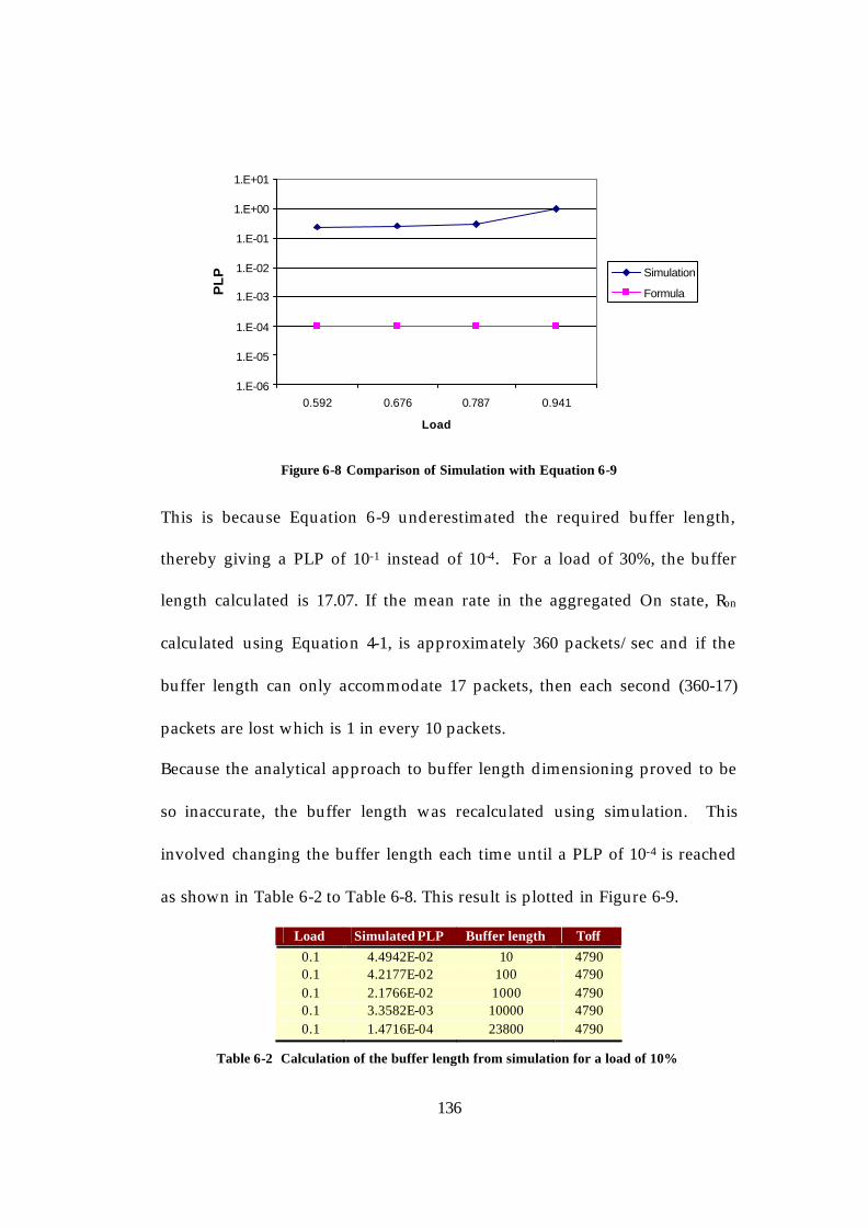
136
1.E-06
1.E-05
1.E-04
1.E-03
1.E-02
1.E-01
1.E+00
1.E+01
0.592 0.676 0.787 0.941
Load
PL
P Simulation
Formula
Figure 6-8 Comparison of Simulation with Equation 6-9
This is because Equation 6-9 underestimated the required buffer length,
thereby giving a PLP of 10-1 instead of 10-4. For a load of 30%, the buffer
length calculated is 17.07. If the mean rate in the aggregated On state, Ron
calculated using Equation 4-1, is approximately 360 packets/sec and if the
buffer length can only accommodate 17 packets, then each second (360-17)
packets are lost which is 1 in every 10 packets.
Because the analytical approach to buffer length dimensioning proved to be
so inaccurate, the buffer length was recalculated using simulation. This
involved changing the buffer length each time until a PLP of 10-4 is reached
as shown in Table 6-2 to Table 6-8. This result is plotted in Figure 6-9.
Load Simulated PLP Buffer length Toff 0.1 4.4942E-02 10 4790 0.1 4.2177E-02 100 4790 0.1 2.1766E-02 1000 4790 0.1 3.3582E-03 10000 4790 0.1 1.4716E-04 23800 4790
Table 6-2 Calculation of the buffer length from simulation for a load of 10%
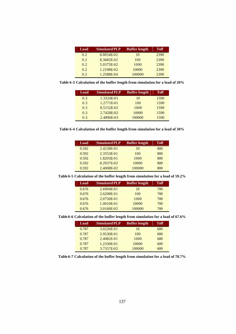
137
Load Simulated PLP Buffer length Toff
0.2 8.8054E-02 10 2390 0.2 8.3682E-02 100 2390 0.2 5.0375E-02 1000 2390 0.2 1.2198E-02 10000 2390 0.2 1.2588E-04 100000 2390
Table 6-3 Calculation of the buffer length from simulation for a load of 20%
Table 6-4 Calculation of the buffer length from simulation for a load of 30%
Load Simulated PLP Buffer length Toff 0.592 2.4238E-01 10 800 0.592 2.3553E-01 100 800 0.592 1.8203E-01 1000 800 0.592 8.2937E-02 10000 800 0.592 2.4008E-02 100000 800
Table 6-5 Calculation of the buffer length from simulation for a load of 59.2%
Load Simulated PLP Buffer length Toff
0.676 2.6904E-01 10 700 0.676 2.6208E-01 100 700 0.676 2.0750E-01 1000 700 0.676 1.0010E-01 10000 700 0.676 3.0160E-02 100000 700
Table 6-6 Calculation of the buffer length from simulation for a load of 67.6%
Load Simulated PLP Buffer length Toff 0.787 3.0226E-01 10 600 0.787 2.9530E-01 100 600 0.787 2.4082E-01 1000 600 0.787 1.2330E-01 10000 600 0.787 3.7357E-02 100000 600
Table 6-7 Calculation of the buffer length from simulation for a load of 78.7%
Load Simulated PLP Buffer length Toff
0.3 1.3324E-01 10 1590 0.3 1.2771E-01 100 1590 0.3 8.5152E-02 1000 1590 0.3 2.7428E-02 10000 1590 0.3 2.4890E-03 100000 1590
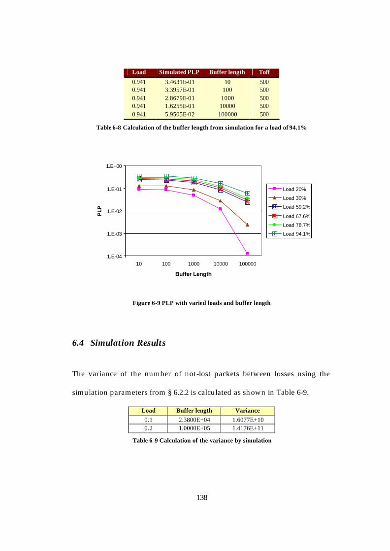
138
Load Simulated PLP Buffer length Toff
0.941 3.4631E-01 10 500 0.941 3.3957E-01 100 500 0.941 2.8679E-01 1000 500 0.941 1.6255E-01 10000 500 0.941 5.9505E-02 100000 500
Table 6-8 Calculation of the buffer length from simulation for a load of 94.1%
1.E-04
1.E-03
1.E-02
1.E-01
1.E+00
10 100 1000 10000 100000
Buffer Length
PL
P
Load 20%
Load 30%
Load 59.2%
Load 67.6%
Load 78.7%
Load 94.1%
Figure 6-9 PLP with varied loads and buffer length
6.4 Simulation Results
The variance of the number of not-lost packets between losses using the
simulation parameters from § 6.2.2 is calculated as shown in Table 6-9.
Load Buffer length Variance 0.1 2.3800E+04 1.6077E+10 0.2 1.0000E+05 1.4176E+11
Table 6-9 Calculation of the variance by simulation
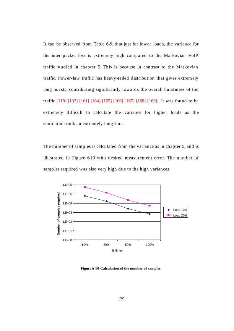
139
It can be observed from Table 6-9, that just for lower loads, the variance for
the inter-packet loss is extremely high compared to the Markovian VoIP
traffic studied in chapter 5. This is because in contrast to the Markovian
traffic, Power-law traffic has heavy-tailed distribution that gives extremely
long bursts, contributing significantly towards the overall burstiness of the
traffic [119] [132] [161] [164] [165] [166] [167] [168] [169]. It was found to be
extremely difficult to calculate the variance for higher loads as the
simulation took an extremely long time.
The number of samples is calculated from the variance as in chapter 5, and is
illustrated in Figure 6-10 with desired measurement error. The number of
samples required was also very high due to the high variances.
1.E+00
1.E+01
1.E+02
1.E+03
1.E+04
1.E+05
1.E+06
10% 20% 50% 100%
% Error
Nu
mb
er o
f sa
mp
les
req
uir
ed
Load 10%
Load 20%
Figure 6-10 Calculation of the number of samples
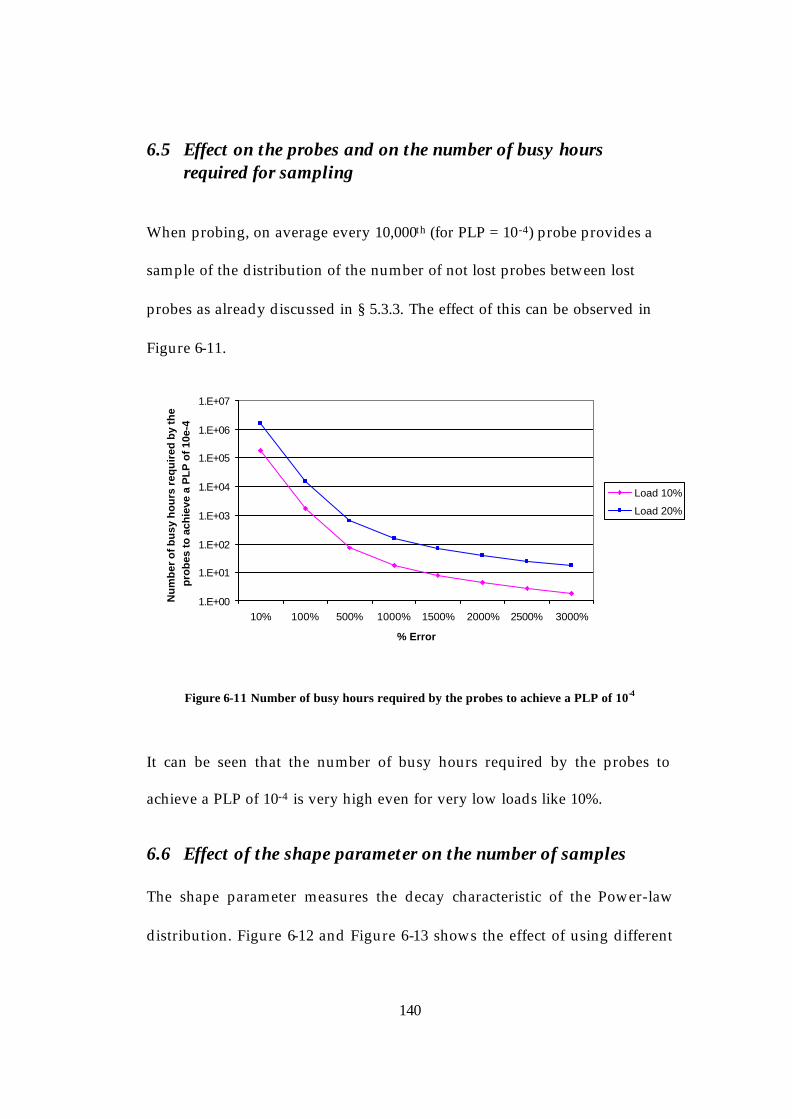
140
6.5 Effect on the probes and on the number of busy hours required for sampling
When probing, on average every 10,000th (for PLP = 10-4) probe provides a
sample of the distribution of the number of not lost probes between lost
probes as already discussed in § 5.3.3. The effect of this can be observed in
Figure 6-11.
1.E+00
1.E+01
1.E+02
1.E+03
1.E+04
1.E+05
1.E+06
1.E+07
10% 100% 500% 1000% 1500% 2000% 2500% 3000%
% Error
Nu
mb
er o
f bu
sy h
ou
rs r
equ
ired
by
the
pro
bes
to a
chie
ve a
PL
P o
f 10e
-4
Load 10%
Load 20%
Figure 6-11 Number of busy hours required by the probes to achieve a PLP of 10-4
It can be seen that the number of busy hours required by the probes to
achieve a PLP of 10-4 is very high even for very low loads like 10%.
6.6 Effect of the shape parameter on the number of samples The shape parameter measures the decay characteristic of the Power-law
distribution. Figure 6-12 and Figure 6-13 shows the effect of using different

141
shape parameters. For a load of 0.1, the buffer length required to get a PLP of
10-4 decreased with increasing shape parameter. This is because the mean
duration of the ON period has decreased with increasing shape parameter.
0 0.5 1 1.5 2 2.5
x 104
10-4
10-3
10-2
10-1
Buffer Limit
PLP
Load 0.1 with shape parameter 1.11Load 0.1 with shape parameter 1.5Load 0.1 with shape parameter 1.7
Figure 6-12 Effect of different shape parameters on the PLP for a load of 0.1

142
0 1 2 3 4 5 6 7 8 9 10
x 104
10-4
10-3
10-2
10-1
Buffer Limit
PLP
Load 0.2 with shape parameter 1.11Load 0.2 with shape parameter 1.5Load 0.2 with shape parameter 1.7
Figure 6-13 Effect of different shape parameters on the PLP for a load of 0.2
Thus, the number of samples required to get a PLP of 10-4 within predefined
measurement error decreases as the shape parameter increases, as illustrated
in Figure 6-14 and 6-15.

143
10 20 30 40 50 60 70 80 90 10010
2
103
104
105
106
% Error
Num
ber
of s
ampl
es r
equi
red
Load 0.1 with shape parameter 1.11Load 0.1 with shape parameter 1.5Load 0.1 with shape parameter 1.7
Figure 6-14 Number of samples required for load of 0.1
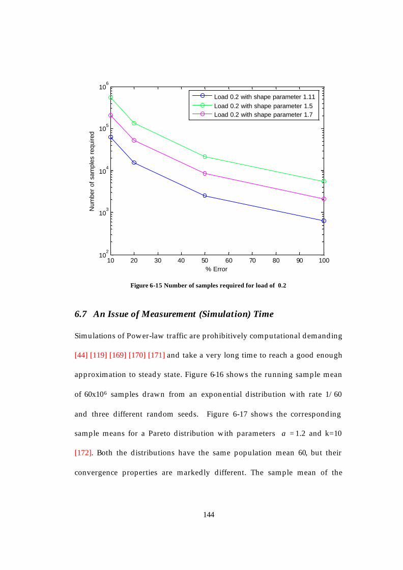
144
10 20 30 40 50 60 70 80 90 10010
2
103
104
105
106
% Error
Num
ber
of s
ampl
es r
equi
red
Load 0.2 with shape parameter 1.11Load 0.2 with shape parameter 1.5Load 0.2 with shape parameter 1.7
Figure 6-15 Number of samples required for load of 0.2
6.7 An Issue of Measurement (Simulation) Time Simulations of Power-law traffic are prohibitively computational demanding
[44] [119] [169] [170] [171] and take a very long time to reach a good enough
approximation to steady state. Figure 6-16 shows the running sample mean
of 60x106 samples drawn from an exponential distribution with rate 1/60
and three different random seeds. Figure 6-17 shows the corresponding
sample means for a Pareto distribution with parameters 2.1=α and k=10
[172]. Both the distributions have the same population mean 60, but their
convergence properties are markedly different. The sample mean of the

145
exponential distribution converges rapidly towards the population mean
after 6000 samples. On the other hand, the sample mean of the Pareto
distribution requires at least 30 million samples to approximate the
population mean. The polynomial tail amplifies the contribution of the large
values to the expectation, and its realisation requires polynomially many
observations and that is why it led to the difficulties of measuring the
variance of the number of not-lost packets between losses for a PLP of 10-4
and for loads greater than about 20%.
Figure 6-16 Running sample mean for exponential distribution with rate 1/60 [172]
Figure 6-17 Running sample mean for Pareto distribution with a=1.2 and k=10 [172]

146
7 Conclusion and Future Work
7.1 Conclusion A novel analytical method was introduced which allowed the prediction of
the number of samples, and hence time required, to accurately measure the
PLP across a networked path, within predefined measured error. This
method was applied to both Markovian and Power-law traffic using FIFO
queue.
The detailed objectives of this research were to develop a novel approach to
discover how probing for PLP across buffered access links is limited, in the
case of both SRD and LRD traffic. The resulting analysis was applied to the
traffic parameters representing a G.711 voice codec. Throughout the thesis,
the buffer length was adjusted accordingly to maintain the target PLP of 10-4.
It was observed that the time for the probes to see an overflowing buffer
increased with increasing load. The mean time taken for the probes to
encounter an overflow was worse for an end-to-end network compared to
buffered access links as the former was traversed across n queues. However,
this analysis is limited because it finds the mean time until a probe first sees
an overflowing buffer. This does not give any measure of the variance of the
overflow process. In chapter 5 an enhanced form of the analysis was

147
developed using the variance of the number of not lost packets between lost
packets was applied to Markovian (VoIP) traffic.
This improved form of the analysis accounted for the inter-packet loss
distribution and hence quantified the number of samples required to
measure the PLP within desired error limits. This is significant as
commercial organizations were legally obliged to monitor the accuracy for
SLA validation. It was shown that the variance of the inter-packet loss
increases with increasing load. This is because the traffic gets burstier w.r.t
the line rate and the queueing gets ‘severe’ as illustrated from Figure 7-1 to
Figure 7-4. It can be seen that as the load increases along with the number of
sources, the knee moves upward, reducing the packet-scale queuing
component and the burst -scale component becomes flatter for Markovian
(VoIP) traffic.
Figure 7-1 Queue State Probability for Load = 69.5%

148
Figure 7-2 Queue State Probability for Load = 79.9%
Figure 7-3 Queue State Probability for Load = 84.5%
Figure 7-4 Queue State Probability for Load = 87.9%
149
Further, it was also shown that the variance of the number of not lost
packets between losses was larger for an end-to-end network when
compared to a single access buffer. Sampling theory stated that the greater
the variability of the sampled data, the more samples was needed for
accurate estimation. Hence the number of samples was increased with
increasing load. An accurate assessment of the measured PLP would need to
account for the statistical requirement to have had N samples of the
distribution being studied. In the case of sampling the distribution of the
number of packets between lost packets, the relation between the values of
N samples of the distribution to the number of probes was investigated. The
number of busy hours calculated using the target PLP 0f 10-4 was very high
and hence made probe based SLA monitoring very difficult for NSPs.
Increasing the PLP allowed to 10-3 had a powerful effect on the burstiness of
the overflow process, and hence its measurability even with lower
bandwidth access links. The key implications for network and service
providers that result from this research are:
• Long periods, i.e. many busy hours, should be allocated to the
collection of packet loss statistics. SLAs should be written on the basis
that “measured PLP” means PLPs averaged over a relatively large
number of busy hours. Further, no guarantees on single busy hours
should be written into legal contracts.

150
• Inaccuracy (measured by increasing number of samples) was highly
load dependent, so network hotspots should be avoided. This implied
that no network node should be allowed, if possible, to experience an
abnormally high level of load as this would tend to both a) create loss
and b) make loss harder to measure.
• The time taken to reach steady state loss statistics was strongly
bandwidth dependent and hence where possible low bandwidth
links, even for access, should be avoided, especially if these low
bandwidth links would tend to be heavily utilized during busy
periods.
It is likely that, particularly mobile and wireless networks, will suffer from
bandwidth bottlenecks even when fixed-wire networks do not. That is why
“buying more bandwidth” is a possible effective solution as more
bandwidth diminishes the unfortunate effects of traffic burstiness. And very
bursty traffic has been found, experimentally, on the current Internet, which
degrades measurement accuracy. This aspect of the problem is indicated
diagrammatically in Figure 7-5: the greater the individual traffic source
burstiness with respect to the channel capacity, the worse the effect on the
measurement accuracy.

151
low speed (access) link, e.g. 256kbps...
12
Nsmall
.
.
.High speed link, e.g. 150Mbps
.
.
.
12
Nlarge
Figure 7-5 diagrammatic representation of the minimising effect on traffic burstiness of higher bandwidth
However, this increase in bandwidth is linked with increased costs, which a
company may not be prepared to pay for, as how the extra bandwidth is
used primarily for the probes.
The variance of the inter-packet loss distribution approach was applied to
Power-law traffic and simulation studies showed that the variance was very
high even at lower loads compared to the Markovian traffic. Due to the
heavy-tailed distribution of the Power-law traffic, there was a major problem
with simulating as the traffic was highly variable. Further problems were
encountered when Equation 6-9 was used to calculate the buffer length so

152
that the PLP of 10-4 could be maintained throughout. This problem was
overcome by using simulation as the means if buffer dimensioning.
Simulations were also run with different shape parameters and lower
variance of the inter-packet loss distribution was observed with increasing
shape parameter. This is due to the increase in the decay rate. Hence the
number of samples required to get a PLP of 10-4 decreased with increasing
shape parameter.
7.2 Future Work There are further issues to consider in relation to packet loss probing and its
accuracy. These are discussed in this section.
This research assumed deterministic probing, however some organisations
have a monitoring strategy that involves releasing probes as batches, rather
than singly. It seems intuitive that such an arrangement will diminish rather
than enhance the accuracy of the measured results, but further work is
required.
It was very difficult to simulate Power-law traffic as it took very long time to
simulate. This is due to the heavy-tailed distribution of the Power-law

153
traffic. But a large number of events are also required to ensure the PLP.
This means that simulation also suffers from the scaling problem. This is
because conventional simulation of packet networks uses a discrete
approach that models each individual packet through the network. This is
called packet -level simulation as each packet’s arrival at, or departure from,
a network element is represented by an event. That is why the simulation for
Power-law traffic resulted in very long simulation times. Much research
work [119] [169] [170] [171] has concentrated on accelerated simulation for
Power-law traffic modelling so that accurate statistics can be collected within
an affordable time. This accelerated simulation technique can be applied to
the model in chapter 6 and the variance of the higher load can possibly be
calculated using these techniques.
In this research, only the On/Off static model was used and hence further
work is necessary on genuinely elastic traffic like TCP. It seems intuitive that
the elastic traffic will be harder to measure.
Finally, the different Classes of Services can be incorporated and then the
PLP measured for each class. The available bandwidth then must be divided
among the different CoS classes. IP Standards now seem to have moved
towards roughly 6 classes of service (Table 3-1), but the 6th class has no
associated performance guarantees, which leaves 5 classes which may need

154
measurement. This will further reduce the number of probes available to
each class, thereby increasing the time until a probe first encounters an
overflowing buffer.
Further work could also be directed to investigating how existing Active
Queue Management (AQM) like WRED may be used to randomize the
sequence of packet drops. It may be that the randomized packet losses are
much easier to measure than those resulting from a tail-drop queue.
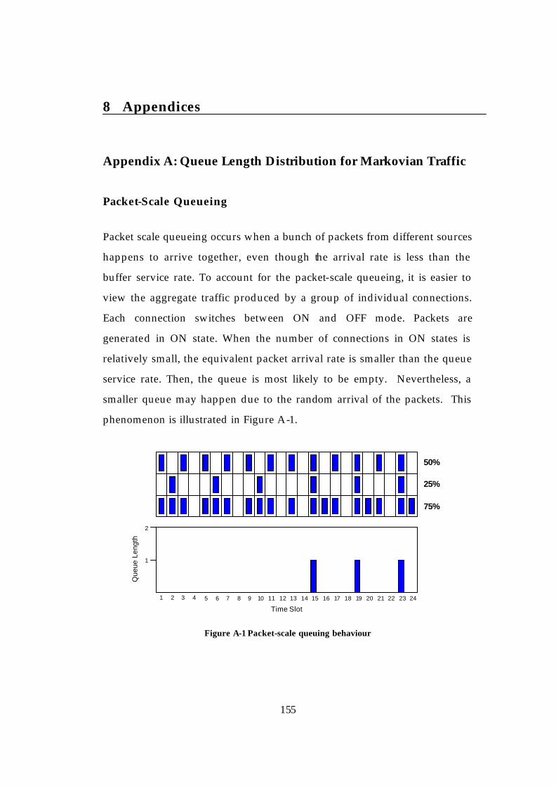
155
8 Appendices
Appendix A: Queue Length Distribution for Markovian Traffic
Packet-Scale Queueing
Packet scale queueing occurs when a bunch of packets from different sources
happens to arrive together, even though the arrival rate is less than the
buffer service rate. To account for the packet-scale queueing, it is easier to
view the aggregate traffic produced by a group of individual connections.
Each connection switches between ON and OFF mode. Packets are
generated in ON state. When the number of connections in ON states is
relatively small, the equivalent packet arrival rate is smaller than the queue
service rate. Then, the queue is most likely to be empty. Nevertheless, a
smaller queue may happen due to the random arrival of the packets. This
phenomenon is illustrated in Figure A-1.
1 2 3 4 5 6 7 8 9 10 11 12 13 14 15 16 17 18 19 20 21 22 23 24
2
1
Time Slot
Que
ue L
engt
h
50%
25%
75%
Figure A-1 Packet-scale queuing behaviour

156
In the example as shown in Figure A-1, there are three connections. The
activity factor of the first, second and third connection are 0.5, 0.25 and 0.75
respectively. Two packets can be removed from the queue during a time slot.
Under this configuration, the load is equal to 0.75. From the diagram, it can
be noted that only a short queue exists; i.e. only packet-scale queuing
behaviour occurs. The small queue is established owing to the random
arrival pattern of the incoming packets.
Burst-Scale Queueing
Burst scale queueing occurs when the aggregate arrival rate exceeds the
buffer service rate, causing the buffer to fill and overflow. The burst scale
queueing is the key factor causing packet loss. Figure A-2 illustrates the
burst-scale queuing effect. Similar to the previous example, two packets can
be served in each time slot. In this example, the third connection has the
activity factor equal to 33% and an extra connection is added with a unity
activity factor, then, the load is as high as 1.041. The equivalent arrival rate is
greater than the service rate. With reference to Figure A-2, it can be noted
that the queue length is gradually built up as indicated by the black solid
line, although some fluctuation is shown.
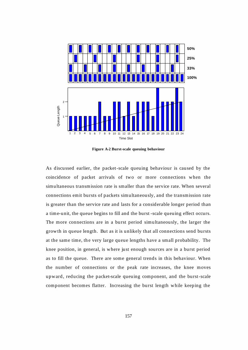
157
1 2 3 4 5 6 7 8 9 10 11 12 13 14 15 16 17 18 19 20 21 22 23 24
2
1
Time Slot
Que
ue L
engt
h
50%
25%
33%
100%
Figure A-2 Burst-scale queuing behaviour
As discussed earlier, the packet-scale queuing behaviour is caused by the
coincidence of packet arrivals of two or more connections when the
simultaneous transmission rate is smaller than the service rate. When several
connections emit bursts of packets simultaneously, and the transmission rate
is greater than the service rate and lasts for a considerable longer period than
a time-unit, the queue begins to fill and the burst -scale queuing effect occurs.
The more connections are in a burst period simultaneously, the larger the
growth in queue length. But as it is unlikely that all connections send bursts
at the same time, the very large queue lengths have a small probability. The
knee position, in general, is where just enough sources are in a burst period
as to fill the queue. There are some general trends in this behaviour. When
the number of connections or the peak rate increases, the knee moves
upward, reducing the packet-scale queuing component, and the burst-scale
component becomes flatter. Increasing the burst length while keeping the

158
load fixed leaves the knee point more or less unchanged but makes the burst
component flatter.
For a FIFO queue multiplexing Markovian traffic used in this thesis, the key
feature of the burst -scale queuing and the packet-scale queuing components
are their exponential decay, i.e. they approximately follow a straight line in
log-linear scale.

159
Appendix B: Comparison of T(ON) with Expected Overflow Duration E(OF)
Results obtained from ns2 simulations (Figure B-1) verify the approximation
in T(ON) with a 95% confidence interval. By constructing 95% confidence
interval about a data point - made by taking the mean and standard
deviation of the individual observations made of the point across multiple
simulation runs, we can note the following: (1) the true mean value of E(OF)
will be between the bars with 95% probability (2) the separation of the bars
will give us an indication of the degree of variability between the trials. If the
variability is large the range of values that the true mean could be is also
large. If the spread is small we are 95% confident that the true mean is
within a very small range of values.
0 0.1 0.2 0.3 0.4 0.5 0.6 0.7 0.8 0.9 110 (̂-2)
10 (̂-1)
10 (̂0)
10 (̂1)
Load
Pro
babi
lity
(sec
s)
95% Confidence IntervalExpected Time for OverflowT[ON]
T[ON]
E[OF]
Figure B-1 Comparison of T[ON] with expected overflow duration E[OF]

160
Appendix C: Calculation of the steady state probability, s(k)
Starting with state 0 (the system is empty), this can be reached from a system
state of either 1 or 0, as shown in Figure C-1. This is saying that the system
can be in state 0 at the end of n-1, with no arrivals in slot n, or it can be in
state 1 at the end of slot n-1, with no arrivals in slot n, and at the end of slot
n, the system will be in state 0. An equation can be written to express this
relationship:
( ) ( ) ( ) ( ) ( )0.10.00 asass += Equation C-8-1
Figure C-8-1 How to reach state 0 at the end of a time slot
s (k) applies as the state probabilities for the end of both time slot n-1 and
time slot n because these are steady-state (sometimes called ‘long-run’)
probabilities, and, on the assumption that the buffer has been active for a
very long period, the probability distribution for the queue at the end of time
slot n-1 is the same as the probability distribution for the end of time slot n.
Thus the Equation C-1 can be rearranged to give a formula for s (1):

161
( ) ( ) ( )( )0
01.01
aa
ss−
= Equation C-2
In a similar way, a formula for s(2) can be found by writing a balance
equation for s(1):
( ) ( ) ( ) ( ) ( ) ( ) ( )0.21.11.01 asasass ++= Equation C-3
Equation C-3 is expressing the probability of having 1 in the queueing
system at the end of slot n, in terms of having 0,1 or 2 in the system at the
end of slot n-1, along with the appropriate number of arrivals as illustrated
in Figure C-2.
Figure C-8-2 How to reach state 1 at the end of a time slot
Thus, any arrivals during the current time slot cannot be served during this
slot. Rearranging the Equation C-3 gives:
( ) ( ) ( ) ( ) ( ) ( )( )0
1.11.012a
asasss −−= Equation C-4
This process can be continued to find a similar expression for the general
state, k

162
( ) ( ) ( ) ( ) ( ) ( ) ( ) ( ) ( ) ( ) ( )0.1.1......2.21.11.01 aksakskasaskasks +−+−++−=− Equation C-5
which, when rearranged gives
( )( ) ( ) ( ) ( ) ( )
( )0
.1.011
1
a
ikaiskasksks
k
i∑
−
=
−−−−−=
Equation C-6

163
Appendix D: Design Rules for Buffering Overlapping Pareto Sources
The duration of the ON periods are Pareto distributed and the duration of
the OFF periods are exponentially distributed. Define first for each of the
individual sources:
Ton = mean ON time of any input process (Pareto distributed ON periods)
h = the data rate output from a source during its ON period
And for the aggregate queueing system (2 state input):
T(on) = mean time the aggregate input process spends in the ON state
(Pareto distributed ON periods)
T(off) = mean time the aggregate input process spends in the OFF state
ρ = load on the queueing system
P(on) = the probability that the aggregate input process is in the ON state
P(off) = the probability that the aggregate input process is in the OFF state
C = the output rate of the queue in data units per / unit time
Ron = mean input rate into the queue when the aggregate input process is
in the ON state
Roff = mean input rate into the queue when the aggregate input process is
in the OFF state
X = the buffer length in data units
A = the mean applied load in data units per unit time
Once reduced to a single 2-state model, it has the following properties: In the
ON state the total input rate exceeds the service rate of the buffer, and the
buffer fills (rate of increase = Ron - C); in the OFF state the total input rate is
less than the output rate of the buffer, so allowing the buffer to empty
(reduction rate = C - Roff). When not less than C/h sources are active at any
time the aggregate process is in the ON state, otherwise it is in the OFF state.

164
Here we use the same simple expressions for the parameters of the 2 state
model This reduces the aggregate model to one of the M/G/1 type, and for
this M/G/1 queue model we now define:
p[k] = P(k data units in the queue at a randomly chosen departure instant
in the aggregate model)
Q(x) = P(queue length >X data units at a randomly chosen unit departure
instant)
= 1 - p[0] - p[1] - … - p[x]
B[k] = P(>k arrivals in a, Pareto distributed, batch) = ξ. k-α
B = the mean number in a (Pareto distributed) batch of arrivals
q = P(a batch arrives in any randomly chosen period between
departures, in the aggregate model)
This gives:
A[k]=P(>k arrivals in a randomly chosen period between departures)=q.B[k]
Because one data unit is the smallest amount of work that can arrive at any
arrival instant we have:
ξ = 1 and α = B/(B-1), or B = α / (α - 1) Also:
q = 1 – exp(-λ) where:
B = T(on).(Ron – C) = Ton.h2.A / (C-A)2 therefore:
λ = ρ / B = ((C-A)2)/(Ton.h2.C) therefore:
A[k] = q.k-α k>0.
The recurrence formula for any queue of the M/G/1 type (using the line
crossing approach) is:

165
[ ] ρ−= 10p Equation D-1
[ ] [ ] [ ]( )q
App−
=1
1.01 Equation D-2
[ ] ( ) [ ] [ ]jAjkpq
kpk
j
.1
1
1∑
=
−−
= for k>1 Equation D-3
( ) [ ]∑=
−=x
j
jpxQ0
1 Equation D-4
We can avoid the use of the recurrence equation approach, and obtain a
simple, closed form solution for predicting the buffer overflow probability in
the original N input queuing scenario. This further simplification fits a
Pareto distribution to the “virtual waiting time probabilities” in the M/G/1
queue. Define the virtual waiting time as:
V[1] = 1 – p[0]
V[2] = 1 – p[0] – p[1] and in general:
V[j] = 1 – p[0] – p[1] - … - p[j] = k.j-b j ≥ 0.
Fitting a Pareto distribution gives:
V[1] = K.1-b = K = 1- p[0] = ρ
V[2] = K.2-b = (1- p[0] – p[1]) therefore:
ρ.2-b = (1- p[0] – p[1])
-b = log2(1- p[0] – p[1]) / ρ) = log2((ρ – p[1]) /ρ)
-b = log2((ρ – (1-ρ)(1-a[0])/a[0]) / ρ)
-b = log2((1 – (ρ-1 - 1)(eλ - 1)) and therefore the buffer overflow
probability is given by:

166
( ) ( )( )
−
−
−= 1exp.1
11log. 2 λ
ρρ XxQ Equation
D-5
Expressing this in terms of the original N source multiplexing scenario:
B = T(on).(Ron – C) = Ton.h2.A / (C-A)2
therefore: λ = ρ / B = ((C-A)2)/(Ton.h2.C)
therefore:
( )( )
−
−
−
−
=1
..exp.111log
2
2
2
.ChT
AC
onXxQρ
ρ Equation
D-6
Which is easily re-arranged for the required buffer length, X.

167
9 Author’s Publications
1 Hasib, M, Schormans, J.A.: "Limitations of Passive and Active Measurement Methods in Packet Networks" London Communications Symposium 2003
2 Hasib M, Schormans J A, and Pitts J M: “Probing limitations for packet loss probability measurement on buffered access links” IEE Electronic Letter Electronics Letters, Volume: 40, Issue: 20, 30 Sept. 2004 Pages: 1315 - 1316
3 Hasib, M, Schormans, J.A.: "Limitations for Measuring Packet Loss Probability using Active Probing Techniques" London Communications Symposium 2004.
4 Hasib M, Schormans J A and Timotijevic, T: “Accuracy of Packet Loss Monitoring over Networked CPE” Submitted to the IEE Communications Proceedings

168
10 References
1. Palmieri, F : “Improving the performance in multimedia streaming networks: a differentiated service approach“, Video/Image Processing and Multimedia Communications, 2003. 4th EURASIP Conference focused on Volume 2, 2 -5 July 2003 Page(s):841 - 849 vol.2
2. P. Crowcroft, J. Kirstein, P. Bhatti, S: “Congestion control mechanisms and the best effort service model”, Gevros, Network, IEEE Volume 15, Issue 3, May-June 2001 Page(s):16 – 26
3. Rouhana, N. Horlait, E: “Differentiated services and integrated services use of MPLS Computers and Communications”, 2000. Proceedings. ISCC 2000. Fifth IEEE Symposium on 3-6 July 2000 Page(s):194 – 199
4. Bakiras, S, Li, V.O.K.: “Quality of service support in differentiated services packet networks”Communications, 2001. ICC 2001. IEEE International Conference on Volume 8, 11-14 June 2001 Page(s):2370 - 2374 vol.8
5. Matta, J, M, Takeshita, A: “End-to-end voice over IP quality of service estimation through router queuing delay monitoring” Global Telecommunications Conference, 2002. GLOBECOM '02. IEEE Volume 3, 17-21 Nov. 2002 Page(s):2458 - 2462 vol.13
6. http://t1rex.blogspot.com/2006/02/managed-ip-services-becoming-network.html
7. www.globalcrossing.com 8. www.cisco.com 9. www.bt.com 10. www.mci.com 11. www.lucent.com 12. www.juniper.net 13. RFC 2212: Specification of Guaranteed Quality of Service 14. Bouman. J, Trienekens. J, Van der Zwan, M: “Specification of service
level agreements, clarifying concepts on the basis of practical research” Software Technology and Engineering Practice, 1999. STEP '99. Proceedings 30 Aug.-2 Sept. 1999 Page(s):169 – 178
15. Verma, D.C: “Service level agreements on IP networks” Proceedings of the IEEE Volume 92, Issue 9, Sep 2004 Page(s):1382 – 1388
16. Timotijevic, T, Leung, C.M. and Schormans, J.A: “Accuracy of measurement techniques supporting QoS in packet based Intranet and Extranet VPNs”. IEE Proceedings Communications Special Edition on VPNs and Broadband Technology Vol. 151, No.1, Feb. 2004.
17. Hasib, M, Schormans, J.A.: "Limitations of Passive and Active Measurement Methods in Packet Networks" London Communications Symposium 2003.

169
18. Barford, P.; Sommers, J: “Comparing Probe-based and router-based Packet-Loss Measurement” Internet Computing, IEEE, Volume: 8, Issue: 5, Sept.-Oct. 2004 Pages: 50 – 56.
19. Hasib M, Schormans J A, and Pitts J M: “Probing limitations for packet loss probability measurement on buffered access links” IEE Electronic Letter Electronics Letters, Volume: 40, Issue: 20, 30 Sept. 2004 Pages: 1315 - 1316
20. Barford, Paul; Sommers, Joel.; A Comparison of Active and Passive Methods for Measuring Packet Loss, UW Technical Report, October, 2002.
21. Asawa, M: “Measuring and analyzing service levels: a scalable passive approach” Quality of Service, 1998. (IWQoS 98) 1998 Sixth International Workshop on 18-20 May 1998 Page(s):3 – 12.
22. Ryoki, N, Kawhara, K., Ikenaga, T and Oie, Y : “Performance analysis of queue length distribution of tandem routers for QoS measurement” Applications and the Internet (SAINT) Workshops, Proceedings 2002 Symposium on 28 Jan.-1 Feb. 2002 Page(s): 82 – 87.
23. C.M. Leung, J.A Schormans: “Measurement-based traffic characteristic estimation for QoS oriented IP networks”, 41st European Telecommunications Congress, Genoa, September 2002.
24. Lindh, T: “Performance Monitoring in Communication Networks” PhD Thesis, Stockholm, 2004
25. J. Cleary, S. Donnelly, I. Graham, A. McGregor, and M. Pearson: “Design principles for accurate passive measurement” Proceedings of PAM2000, Hamilton, New Zealand, April 2000.
26. Leung,C.M, Schormans,J.A., Pitts,J.M, Woolf,A: "Accurate decay rate prediction for burst-scale queueing in packet buffers", Electronic Letter, Volume: 39 Issue:2, 23 Jan 2003, Page(s):253-254
27. Cleary, J, Graham, I, McGregor, T, Pearson, M.; Ziedins, L.; Curtis, J.; Donnelly, S.; Martens, J.; Martin, S: “High precision traffic measurement” Communications Magazine, IEEE Volume 40, Issue 3, March 2002 Page(s):167 – 173
28. Pasztor, A, Veitch, D: “A precision infrastructure for active probing” Proceedings of the PAM2001 Workshop on Passive & Active Measurements, Amsterdam, Apr.2001.
29. Shanlunov, S, Teitelbaum, B, Karp, A, Boote, J, W, Zekauskas, M: “A One-Way Delay Measurement Protocol (OWAMP)” Internet Draft May 2003.
30. Changhua Z; Changxing P; Yunhui Y; Dongxiao Q: ”Active Probe of Available Bandwidth: Analysis and Improvement” Parallel and Distributed Computing, Applications and Technologies, 2005. PDCAT 2005. Sixth International Conference on 05-08 Dec. 2005 Page(s):134 - 138

170
31. Labit, Y.; Owezarski, P.; Larrieu, N: “Evaluation of active measurement tools for bandwidth estimation in real environment” End-to-End Monitoring Techniques and Services, 2005. Workshop on 15 May 2005 Page(s):71 – 85
32. Schormans, J.A.; Pitts, J.M.: “So you think you can measure IP QoS?” Telecommunications Quality of Services: The Business of Success, 2004. QoS2004.IEE 2-3 March 2004 Page(s):151 - 155
33. Huffaker, B.; Plummer, D.; Moore, D.; Claffy, K: ”Topology discovery by active probing” Applications and the Internet (SAINT) Workshops, 2002. Proceedings. 2002Symposiumon28 Jan.-1 Feb. 2002 Page(s):90 - 96
34. “Service-Level Management: Defining and Monitoring Service Levels in the Enterprise”CiscoWhitePaper,2003http://www.cisco.com/en/US/products/sw/cscowork/ps2428/products_white_paper09186a0080091ba5.shtml
35. Cooperative Association for Internet Data Analysis (CAIDA): http://www.caida.org/tools/measurement/skitter
36. National Laboratory for Applied Network Research (NLANR): http://www.moat.nlanr.net
37. Hill, J.: “Assessing the Accuracy of Active Probes for Determining Network Delay, Jitter and Loss”. MSc Thesis in High Performance Computing, The University of Edinburgh, 2002.
38. Bolot., J: “End-to-end packet delay and loss behavior in the Internet” Proceedings of ACM SIGCOMM ’93, San Francisco, September 1993.
39. Schormans, J.A. and Timotijevic, T.: “Evaluating the Accuracy of Active Measurement of Delay and Loss in Packet Networks”, 6th IFIP/IEEE International Conference on Management of Multimedia Networks and Services, September 2003, Queens University, Belfast
40. Timotijevic, T. and Schormans, J.A.: “Bandwidth overhead of probe technology guaranteeing QoS in packet networks”. IEE Electronics Letters, 15th May, 2003, Vol. 39, No. 10, pp 816-818.
41. Roughan, M: “Fundamental bounds on the accuracy of Network Performance Measurements” Joint International Conference on Measurement and Modeling of Computer Systems archive Proceedings of the 2005 ACM SIGMETRICS international conference on Measurement and modeling of computer systems , pages 253-264 , Banff, Alberta, Canada 2005
42. Sommers, J, Barford, P, Duffield, N and Ron, A: “Improving accuracy in end-to-end packet loss measurement” Proceedings of ACM SIGCOMM, August, 2005
43. Gochran, W: “Sampling Techniques” John Wiley and Sons, 1966
44. Pitts, J.M. and Schormans, J.A.: “Introduction to IP and ATM Design and Performance”, Wiley, December 2000.
171
45. M. Karam, F. Tobagi, “Analysis of the delay and jitter of voice traffic over the Internet,” Proceedings of INFOCOM’OI. April 2001.
46. Brownlee, Nevil; Lossley Chris.; Fundamentals of Internet Measurement: A Tutorial, Keynote Systems, 2001.
47. Frogner, B.; Cannara, A.B.; Monitoring and Prediction of Network Performance, Advance Issues of E-Commerce and Web-Based Information Systems, WECWIS, 1999. International Conference on , 8-9 April 1999, Page(s): 122 -129
48. ITU Recommendation Y.154 49. Meky ,Saadawi: “Degredation Effect of Cell Loss on Speech Quality over
ATM Networks”, in Broadband Communication Ed. Mason & Canaca, pub. By Chapman & Hall, 1996.
50. Oodan A, Ward K, Savolaine C, Daneshmand M, Hoath P: “Telecommunications Quality of Service Management from legacy to emerging services” IEE Telecommunications Series 48, 2003.
51. Hong, J.; Traffic Measurement for High-Speed Internet, 2003 ICAT Workshop, Seoul, Korea, Apr. 2003
52. D. Verma, “Support Service Level Agreement on IP network”, Macmillan Technology Series, 1999
53. R. Sprenkels, A. Pras, “Service Level Agreements”, Internet NG, WU2, D2.7,Apr. 2001 available at http://ing.ctit.utwente.nl/WU2/
54. “Service Level Management: Best Practices White Paper” available at http://www.cisco.com/warp/public/126/sla.htm
55. TeleManagement Forum – SLA Management Handbook, GB 915, June 2001
56. H. Joachim “Differentiated Services – Network Configuration and Management:Network Control, Measurement and Charging for Service Models” EURESCOM Project P1006 EDIN 0065-10006 Jan. 2001
57. Mullins M “Beyond availability: improving service performance”, IEE Information Professional June/July 2004
58. SAA home page: http://www.cisco.com/go/saa 59. Kumar, V.P.; Lakshman, T.V.; Stiliadis, D: “Beyond best effort: router
architectures for the differentiated services of tomorrow's Internet” Communications Magazine, IEEE Volume 36, Issue 5, May 1998 Page(s):152 – 164
60. Haeryong L; Jeongyeon H; Byungryong K; Kyoungpyo J: “ End-to-end QoS architecture for VPNs: MPLS VPN deployment in a backbone network” Parallel Processing, 2000. Proceedings. 2000 International Workshops on 21-24 Aug. 2000 Page(s):479 – 483
61. International Organization for Standardization: www.iso.org 62. Subramanian M; Network Management – Principles and Practice,
Addison Wesley, 2001
172
63. Case, J.D: “Management of high speed networks with the simple network management protocol (SNMP) Local Computer Networks”, 1990. Proceedings., 15th Conference on 30 Sept.-3 Oct. 1990 Page(s):195 – 199
64. Simple Network Management Protocol: http://www.cisco.com/univercd/cc/td/doc/cisintwk/ito_doc/snmp.htm
65. Leung, C.M: “Non-Intrusive Measurement in Packet Networks and its Applications”, PhD Thesis, University of London, 2004
66. Floyd, S.; Jacobson, V.; Random early detection gateways for congestion avoidance, IEEE/ACM Transactions on Networking, vol. (1), pp. 397-413, Aug. 1993
67. Cisco – Measuring Delay, Jitter, and Packet Loss with Cisco IOS SAA and RTTON available from http://www.cisco.com/warp/public/126/saa.pdf
68. Juniper Networks; Juniper enterprise specific Class-Of-Service (COS) MIB, 2002, available from http://www.juniper.net/techpubs/software/junos/junos57/swconfig57-net-mgmt/html/mib-jnx-cos.txt
69. Luckie J M, McGregor A J, Braun H : “Towards improving packet probing techniques” ACM SIGCOMM Internet Measurement Workshop, Nov. 2001
70. Moon. B.S : PhD Thesis: “Measurement and Analysis of End-to-End Delay and Loss in the Internet” University of Massachusetts Amherst 2000
71. http://e2epi.internet2.edu/owamp/
72. Internet Engineering Task Force: http://www.ietf.org/
73. Internet Protocol Performance Metric: http://www.advanced.org/IPPM/
74. ITU-T Recommendation: G.711
75. McGregor, T: “Quality in measurement: beyond the deployment barrier Applications and the Internet” (SAINT) Workshops, 2002. Proceedings. 2002 Symposium on 28 Jan.-1 Feb. 2002 Page(s):66 – 73
76. Caceres, R.; Duffield, N.G.; Horowitz, J.; Towsley, D.; Bu, T.; “Multicast-Based Inference of Network Internal Characteristics: Accuracy of Packet Loss Estimation”, IEEE INFOCOMM’99, Mar. 1999
77. Padmanadhan, V.N.; Lili, Q.; Wang, H.J.; “Server-based inference of internet link lossiness”, IEEE INFOCOM’03, vol. 1, pp. 145-155, 2003

173
78. Presti, F.L.; Duffield, N.G.; “Multicast-Based Inference of Network-Internal Delay Distributions”, Preprint AT&T Laboratories and University of Massachusetts
79. Coates, M.; Nowak, R.; “Network Tomography for Internal Delay Estimation” , IEEE International Conference on Acoustics, Speech, and Signal Processing, May, 2001
80. NONPARAMETRIC INTERNET TOMOGRAPHY: http://www.ngi-supernet.org/NGI-PI-2001/Towsley.pdf
81. Duffield, N.G, Horowitz. J, Presti, F.L, and Towsley, D: “Network Delay Tomography from End-to-end Unicast Measurements” Proceedings of the 2001 International Workshop on Digital Communications 2001- Evolutionary Trends of the Internet, Taormina, Italy, September 17-20, 2001
82. Jamin.S, Shenker, S.J and Danzig, P.B “Comparison of Measurement-based Admission Control Algorithms for Controlled-Load Service” Proceedings of the Conference on Computer Communications (IEEE Infocom), (Kobe, Japan), Apr. 1997. INFOCOM '97. pp. 973
83. Breslau, L.; Knightly, E.; Shenker, S.; Stoica, I.; Zhang, H.; “Endpoint Admission Control: Architectural Issues and Performance”, Proc. ACM SIGCOMM 2000, Aug. 2000
84. V. Fodor, G. Karlsson, and R. Ronngren, “Admission control based on end–to–end measurements,” in Proc. of the 19th Infocom, (Tel Aviv, Israel),pp. 623–630, IEEE, March 2000.
85. Ferrari, T, Almesberger W., and Le Boudec J.-Y., “SRP: a scalable resource reservation protocol for the Internet,” in Proc. of the 6th IWQoS, LNCS, (Napa, CA),pp. 107–116, Springer, May 1998.
86. Gibbens, R. J. and Kelly, F. P. “Measurement-based connection admission control,”in Proc. of the 15th International Teletraffic Congress, (Washington D.C., USA),pp. 879–888, June 1997.
87. Mortier, R. Pratt, I. Clark, C and Crosby S, “Implicit admission control,” IEEE Journal on Selected Areas in Communications, vol. 18, no. 12, pp. 2629–2639, 2000.
88. Kelly, F. P, Key, P. B and Zachary. S, “Distributed admission control,” IEEE Journal on Selected Areas in Communications, vol. 18, no. 12, pp. 2617–2628,2000.
89. Crosby, S., Leslie, I., Mcgurk, B., Lewis, J. T., Russell, R., and Toomey, F: “Statistical properties of a near-optimal measurement based cac algorithm”, In Proceedings IEEE ATM ’97 (June 1997).
90. Dziong, Z., Juda, M., and Mason, L: “A framework for bandwidth management in ATM networks – aggregate equivalent bandwidth estimation approach”, IEEE/ACM Transactions on Networking 5, 1 (Feb. 1997),134–147.
174
91. Floyd, S: “Comments on measurement-based admissions control for controlled-load services”, Technical report, Lawrence Berkeley Laboratory, July 1996.
92. Gibbens, R., and Kelly, F. “Measurement-Based Connection Admission Control”. 15th International Teletraffic Congress (Jun. 1997).
93. Gibbens, R. J., Kelly, F. P., and Key, P. B: “A decision-theoretic approach to call admission control in ATM networks” IEEE Journal on Selected Areas in Communications SAC-13, 6 (1995), 1101–1113.
94. Grossglauser, M., And Tse, D: “A framework for robust measurement-based admission control” Computer Communications Review 27, 4 (Oct. 1997), 237–248. ACM SIGCOMM’97, Sept. 1997.
95. Grossglauser, M., and Tse D. N. C., “A time-scale decomposition approach to measurement-based admission control” In Proceedings of the Conference on Computer Communications (IEEE Infocom) (New York, Mar. 1999).
96. Grossglauser, M, Tse, D. N. C. C Kurose, J., and Towsley, D: “A new algorithm for measurement-based admission control in integrated services packet networks” In Proceedings of the Fifth International Workshop on Protocols for High-Speed Networks (Antipolis, France, Oct. 1996).
97. Jamin, S., Danzig, P. B., Shenker, S. J., and Zhang, L.: “A measurement-based admission control algorithm for integrated services packet networks” IEEE/ACMTransactions on Networking 5, 1 (Feb. 1997), 56–70.
98. Jamin, S., Shenker, S., and Danzig, P. “Comparison of Measurement-based Admission Control Algorithms for Controlled-Load Service”. Proceedings of the Conference on Computer Communications (IEEE Infocom)’97 (Apr. 1997).
99. Knightly, E. W., And Qiu, J: “Measurement-based admission control with aggregate traffic envelopes”, In IEEE ITWDC ’98 (Ischa, Italy September 1998).
100. Karlsson, G “Providing quality for internet video services,” in Proc. Of CNIT/IEEE ITWoDC 98, (Ischia, Italy), pp. 133–146, September 1998.
101. Bianchi,G Capone, A and C. Petrioli.C, “Throughput analysis of end–to–end measurement-based admission control in IP,” in Proc. of the 19th Infocom, (Tel Aviv, Israel), pp. 1461–1470, IEEE, March 2000.
102. Mase, K.; Toyama, Y: “End-to-end measurement based admission control for VoIP networks”, Communications, 2002. ICC 2002. IEEE International Conference on Volume 2, 28 April-2 May 2002 Page(s):1194 - 1198 vol.2
103. Breslau, L, Knightly. E, Shenker, S and Stoica. I , “Endpoint admission control: Architectural issues and performance,” In Proc. ACM SIGCOMM, 2000

175
104. Tuan,T and Park,K “Multiple time scale congestion control for self-similar network traffic,” in Performance Evaluation, vol. 36, pp. 359–386, 1999.
105. “Real-timeSLAmonitoringtools.” http://www.nwfusion.com/news/tech/2001/0115tech.html.
106. Ribeiro,V ,Coate. M., Riedi, R, Sarvotham, S, Hendricks,B, and Baraniuk,R, “Multifractal cross -traffic estimation,” Proc. of ITC Specialist Seminar on IP Traffic Measurement, Sept. 2000.
107. Hu. N and Steenkiste, P: “Evaluation and Characterization of Available Bandwidth Probing Techniques” IEEE JSAC Special Issue in Internet and WWW Measurement, Mapping, and Modeling, 2003.
108. Strauss.J, Katabi.D and Kaashoek.F, “A Measurement study of available bandwidth estimation tools,” IMC 2003
109. Ribeiro,V, Riedi,R ,Baraniuk, R ,Navratil,J and Cottrell,L: “pathChirp: Efficient Available Bandwidth Estimation for Network Paths”, Passive and Active Measurement Workshop 2003
110. Melander,B, Bjorkman, M and Gunningberg,P, “A new end-to-end probing and analysis method for estimating bandwidth bottlenecks,” Global Internet Symposium, 2000.
111. http://channels.lockergnome.com/it/archives/20051102_rtcp_realtime_control_protocol_voip_explained.phtml
112. Volner,R: “ATN network- Basic traffic models for services” Transportation and telecommunication in the 3 rd millennium
113. Paxson, V and Floyd, S: “Wide area traffic: the failure of Poisson modelling” Networking, IEEE/ACM Transactions on Volume 3, Issue 3, June 1995 Page(s):226 - 244
114. Ogura, H: “Orthogonal functionals of the Poisson process” Information Theory, IEEE Transactions on Volume 18, Issue 4, Jul 1972 Page(s):473 - 481
115. Krishnan, R.; Silvester, J.A, “Resource allocation in broadband networks-cell, burst or connection level?” Communications, 1994. ICC 94, SUPERCOMM/ICC '94, Conference Record, Serving Humanity through Communications. IEEE International Conference on 1-5 May 1994 Page(s):86 - 90 vol.1
116. Elhanany, I.; Sadot, D, “Queueing analysis of Markov modulated ON/OFF arrivals with geometric service times” Electrical and Electronics Engineers in Israel, 2002. The 22nd Convention of 1 Dec. 2002 Page(s):189 - 191
117. Heffes, H.; Lucantoni, D.; A Markov Modulated Characterization of Packetized Voice and Data Traffic and Related Statistical Multiplexer Performance, IEEE JSAC, pp. 856-868 Sept. 1986

176
118. Nikolaidis, I.; Akyildiz, I.; Source Characterization and Statistical Multiplexing in ATM networks, Technical Report, GIT-CC 92-94, Georgia Tech., 1992
119. Ho. I Ma: “Accelerated Simulation of Power-Law Traffic in Packet Networks”, PhD Thesis, University of London, 2003
120. Stewart, R: “End-to-end delay analysis for small/medium scale IP networks”, PhD Thesis, University of London, 2002
121. Leland, W.; et al.; On the Self-Similar Nature of Ethernet Traffic (Extended Version), IEEE/ACM Trans. Networking, pp. 1-15, Feb. 1994
122. Klivanski, S.; Mukherjee, A.; Song, C.; On Long-Range Dependence in NSFNET Traffic, Technical Report GIT-CC-94-61, Georgia Tech., 1994
123. Crovella, A.; Bestavros, A.; Explaining World Wide Web Traffic Self-Similarity, Technical Report TR-95-015, 1995
124. Garrett, M; Willnger, W.; Analysis, Modeling and Generation of Self-Similar VBR Video Traffic, Proc. SIGCOMM ’94, Aug. 1994
125. Fong, S.; Singh, S, “Performance evaluation of shared-buffer ATM switches under self-similar traffic Performance”, Computing, and Communications Conference, 1997. IPCCC 1997., IEEE International 5-7 Feb. 1997 Page(s):252 - 258
126. Mehrpour, L.H.; Ambikairajah, E: “Cell loss analysis of self-similar traffic in ATM network”, Circuits and Systems, 2002. APCCAS '02. 2002 Asia-Pacific Conference on Volume 2, 28-31 Oct. 2002 Page(s):457 - 460 vol.2
127. Gao,L, Wang,Z, Zheng,X,J: “Traffic measurement algorithm for self-similar traffic based on probability admission mechanism” Machine Learning and Cybernetics, 2004. Proceedings of 2004 International Conference onVolume 5, 26-29 Aug. 2004 Page(s):2719 - 2724 vol.5
128. Yang,X, Petropulu, A.P.; Adams, V: ”The extended on/off process for modeling traffic in high-speed communication networks” Statistical Signal and Array Processing, 2000. Proceedings of the Tenth IEEE Workshop on 14-16 Aug. 2000 Page(s):495 – 499
129. Addie, R.G.; Neame, T.D.; Zukerman, M: “Modeling superposition of many sources generating self similar traffic” Communications, 1999. ICC '99. 1999 IEEE International Conference on Volume 1, 6 -10 June 1999 Page(s):387 - 391 vol.1
130. Michiel, H.; Laevens, K.; Teletraffic engineering in a broad -band era, Proceedings of the IEEE, vol. 85, pp. 2007-2003, Dec. 1997
131. O’Mahony, M, J, Simeonidou, D, Hunter, D, K, and Tzanakaki, A: “The application of optical packet switching in future communication networks” IEEE Commun. Mag, 2001, 39 (3) pp 128-135

177
132. Crovella, M, E and Bestavros, A : “Self-similarity in worldwide web traffic: evidence and possible causes” ACM Sigmetrics’96 May 1996, Philadelphia, USA, pp. 160-169.
133. Bhadra, A, Sadiku, M, N, O: “Simulation of an ATM network using on-off model” Proc. of the IEEE, pp. 467-470, Apr. 2000.
134. Han, W, Y, Lee, S, J, Han, C, M, Kim, S, H: “Queueing analysis for an ATM multiplexer loaded by CBR and On/Off traffic sources” Singapore ICCS’94, pp. 760-764, Nov. 1994.
135. Galmes, S.; Puigjaner, R: “On the capabilities of on-off models to capture arbitrary ATM sources” INFOCOM '98. Seventeenth Annual Joint Conference of the IEEE Computer and Communications Societies. Proceedings. IEEE Volume 3, 29 March-2 April 1998 Page(s):1333 - 1340 vol.3
136. Moscholios, I.D.; Logothetis, M.D.; Koukias, M.N: “An ON-OFF multi-rate loss model with a mixture of service-classes of finite and infinite number of sources”, Communications, 2005. ICC 2005. 2005 IEEE International Conference on Volume 1, 16-20 May 2005 Page(s):357 - 362 Vol. 1
137. Garroppo, R.G.; Giordano, S.; Isopi, M.; Pagano, M: “On the implications of the off periods distribution in two-state traffic
models “ Communications Letters, IEEE Volume 3, Issue 7, July 1999 Page(s):220 - 222 138. Oliveira, A.L.I.; Monteiro, J.A.S, “Statistical multiplexing of
aggregate data traffic in ATM networks” Telecommunications Symposium, 1998. ITS '98 Proceedings. SBT/IEEE International 9-13 Aug. 1998 Page(s):108 - 113 vol.1
139. Jing,Z, Li,L Sun,H: “Performance analysis of congestion control mechanism for ABR service in the presence of background traffic” Communication Technology Proceedings, 1998. ICCT '98. 1998 International Conference on 22-24 Oct. 1998 Page(s):424 - 428 vol.1
140. Roberts, J. (Ed.): 'Performance evaluation and design of multiservice networks’. COST224, Final 1991
141. Schormans J A., and Pitts, J.M.: 'From Erlangs to excess rate', J ; IBTE, October-December 2001
142. Muppala, J.K.; Bancherdvanich, T.; Tyagi, A: “VoIP performance on differentiated services enabled network”, Networks, 2000. (ICON 2000). Proceedings. IEEE International Conference on 5-8 Sept. 2000 Page(s):419 – 423
143. Estepa, A.; Estepa, R.; Vozmediano, J: “A new approach for VoIP traffic characterization” Communications Letters, IEEE Volume 8, Issue 10, Oct. 2004 Page(s):644 – 646

178
144. Yamada, H.; Higuchi, N: “Voice quality evaluation of IP-based voice stream multiplexing schemes” Local Computer Networks, 2001. Proceedings. LCN 2001. 26th Annual IEEE Conference on 14-16 Nov. 2001 Page(s):356 - 364
145. Yamada, H.; Higuchi, N: “On traffic characteristics and bandwidth requirements of voice over IP applications” Computers and Communication, 2003. (ISCC 2003). Proceedings. Eighth IEEE International Symposium on 2003 Page(s):1324 - 1330 vol.2
146. Klepec, B.; Kos, A: “Performance of VoIP applications in a simple differentiated services network architecture” EUROCON'2001, Trends in Communications, International Conference on. Volume 1, 4-7 July 2001 Page(s):214 - 217 vol.1
147. Koole,G.M and Liu.Z: “Stochastic bounds for queueing systems with multiple on-off sources”, Probability in the Engineering and Informational Sciences, Vol. 12, pp. 25-48, Jan. 1998.
148. Qiang F, White, L: “The impact of background traffic on TCP performance over indirect and direct routing”, Communication Systems, 2002. ICCS 2002. The 8th International Conference on Volume 1, 25-28 Nov. 2002 Page(s):594 - 598 vol.1
149. Schulzrinne H, Kurose,J.F and Towsley,D.F: "Loss Correlation for Queues with Single and Multiple Input Streams", Department of Computer Science, University of Massachusetts, Amherst, Massachusetts, Technical Report TR 92-53, July 1992
150. Hao F. Nikolaidis I. Zegura EW., “Efficient simulation of ATM networks with accurate end -to-end delay statistics”, Conference Record of 1998 IEEE International Conference on Communications, pp. 1799-1804, June 1998
151. Schormans, J.; Liu, E.; Cuthbert, L.; Stoneley, G: “Analytic technique for accelerating simulation of generic network traffic”, Electronics Letter Volume 35, Issue 25, 9 Dec. 1999 Page(s):2168 – 2170
152. Claffy, K.C., Polyzos, G.C., and Braun, H-W: “Application of sampling methodologies to network traffic characterisation”. SIGCOMM 1993, 194–203, and also from: citeseer.nj.nec.com/claffy93application.html
153. Notes on Sampling Theory: www.wfu.edu/~cottrell/ecn215/sampling.pdf
154. A. M. Odlyzko, "The Internet and other networks: Utilization rates and their implications, " Information Economics & Policy, 12 (2000), pp. 341-365. (Presented at the 1998 Telecommunications Policy Research Conference.)Also available at :http://www.dtc.umn.edu/#odlyzko/doc/recent.html
155. http://www.btglobalservices.com/business/global/en/customer_zone/customer_service_experience.html

179
156. Park. K and Willinger. W: “Self-similar network traffic and performance evaluation” John Wiley & Sons Inc, USA, 2000
157. Park. K, Kim. G and Crovella. M: “On the relationship between file sizes, transport protocols and self-similar network traffic”, ICNP’96, Oct 1996, Columbus, USA, pp. 171-180
158. Ariffin, S.H.S “Accelerated Simulation for Packet Buffer with Non FIFO Scheduler”, PhD Thesis.2004, Queen Mary, University of London
159. Mondragon R. J., Arrowsmith D.K. and Pitts J.M., “Chaotic Maps for Traffic Modelling and Queuing Performance Analysis”, Performance Evaluation, 2001, 43, pp. 223-240.
160. Samuel L. G., “The application of non linear Dynamics to Tele traffic Modelling”, PhD. Thesis, 1999, Queen Mary , University of London.
161. Pruthi,P.; Erramilli, A “Heavy-tailed on/off source behavior and self-similar traffic” Communications, 1995. ICC 95 Seattle, Gateway to Globalization, 1995 IEEE International Conference on Volume 1, 18-22 June 1995 Page(s):445 - 450 vol.1
162. Definition of Optimum Traffic Control Parameters and Results of Trials; EXPERT Deliverable 15; AC094/EXPERT/WP41/DS/R/P/015/B1 pp. 6
163. Schormans, J.A, Pitts, J.M, Scharf, E.M, Pearmain A.J and Phillips, C.I : “Design rules for buffering overlapping Pareto processes in packetised networks “ Electronics Letters, 2000 vol. 36, pp. 1086-1088
164. Beran J., Sherman R, Taqqu M. S. And Willinger W., “Long-Range Dependence in Variable-Bit-Rate Video Traffic”, IEEE Transactions on Communications, 43, (2/3/4), February/March/April 1995.
165. Erramilli,A ,Gosby, D and Willinger, W, “Engineering for Realistic Traffic: A Fractal Analysis of Burstiness”, Proc of Special ITC Seminar, Bangalore, India, 1993.
166. Erramilli,A and Willinger,W, “Fractal Properties in Packet Traffic Measurements”, Proc. of ITC Regional Seminar, St. Petersburg 1993.
167. Leland W.E and Wilson, D.V, “High Time Resolution measurements and Analysis of LAN Traffic: Implications for LAN Interconnection,” Proc. of IEEE INFOCOM ‘91, Bal Harbor, FL, 1991.
168. Meier-Hellstern,K,Wirth, P, Yan, Y.L and Hoeflin,D: “Traffic Models for ISDN Data Users: Office Automation Application,'' Proc. ITC-13, Copenhagen, 1991.
169. Deman, S.W and Boel, R.K: “Importance sampling techniques for the estimation of CLR and its sensitivity” AEU-Int J. Electron. Commun, 1998, 52, (3), pp. 141-151
170. Ariffin, S.H.S and Schormans, J.A: “On/Off Pareto distributed source at Burst Level: A Study of Fast Simulation Methods for packet networks” PGNET’02, Apr 2002, Liverpool, U.K

180
171. Li, J.S, Wolisz, A and Popescu-Zeletin, R: “Fast Simulation of self-similar traffic”, IEEE ICC’98, June 1998, Atlanta, USA, pp. 1829-1833
172. Park. K and Willinger. W: “The Internet as a large-scale complex system” oxford University Press, 2005