analysis of radome-enclosed antennas
TRANSCRIPT

8/20/2019 Analysis of Radome-Enclosed Antennas
http://slidepdf.com/reader/full/analysis-of-radome-enclosed-antennas 1/319

8/20/2019 Analysis of Radome-Enclosed Antennas
http://slidepdf.com/reader/full/analysis-of-radome-enclosed-antennas 2/319
Analysis of Radome-Enclosed Antennas
Second Edition

8/20/2019 Analysis of Radome-Enclosed Antennas
http://slidepdf.com/reader/full/analysis-of-radome-enclosed-antennas 3/319
For a listing of related Artech House in the, Antennas and Propagation Series
turn to the back of this book.

8/20/2019 Analysis of Radome-Enclosed Antennas
http://slidepdf.com/reader/full/analysis-of-radome-enclosed-antennas 4/319
Analysis of Radome-Enclosed Antennas
Second Edition
Dennis J. Kozakoff
a r techhouse . com

8/20/2019 Analysis of Radome-Enclosed Antennas
http://slidepdf.com/reader/full/analysis-of-radome-enclosed-antennas 5/319
Library of Congress Cataloging-in-Publication Data A catalog record for this book is available from the U.S. Library of Congress.
British Library Cataloguing in Publication Data A catalogue record for this book is available from the British Library.
Cover design by Greg Lamb
ISBN 13: 978-1-59693-441-2
© 2010 ARTECH HOUSE, INC.685 Canton Street
Norwood, MA 02062
All rights reserved. Printed and bound in the United States of America. No part of this book may be reproduced or utilized in any form or by any means, electronic or mechanical, includ-ing photocopying, recording, or by any information storage and retrieval system, without per-mission in writing from the publisher.
All terms mentioned in this book that are known to be trademarks or service marks havebeen appropriately capitalized. Artech House cannot attest to the accuracy of this information.Use of a term in this book should not be regarded as affecting the validity of any trademark or service mark.
10 9 8 7 6 5 4 3 2 1
Disclaimer:
This eBook does not include the ancillary media that was
packaged with the original printed version of the book.

8/20/2019 Analysis of Radome-Enclosed Antennas
http://slidepdf.com/reader/full/analysis-of-radome-enclosed-antennas 6/319
Contents
Foreword xiii
Preface xv
Acknowledgments xix
Part I: Background and Fundamentals 1
1 Overview of Radome Phenomenology 3
1.1 History of Radome Development 3
1.2 Radome-Antenna Interaction 5
1.2.1 Boresight Error (BSE) and Boresight Error Slope (BSES) 6
1.2.2 Registration Error 7
1.2.3 Antenna Sidelobe Degradation 7
1.2.4 Depolarization 7
1.2.5 Antenna Voltage Standing Wave Ratio (VSWR) 8
1.2.6 Introduction of an Insertion Loss Due to the Presence
of the Radome 8
1.3 Significance of Parameters in Radome Performance 8
1.4 Radome Technology Advances Since the First Edition 10
v

8/20/2019 Analysis of Radome-Enclosed Antennas
http://slidepdf.com/reader/full/analysis-of-radome-enclosed-antennas 7/319
1.4.1 Use of Metamaterials 10
1.4.2 Frequency Selective Radomes 11
1.4.3 Concealed Radomes 12
References 13
2 Basic Principles and Conventions 15
2.1 Vector Mathematics 15
2.2 Electromagnetic Theory 18
2.3 Matrices 21
2.4 Coordinate Systems and Gimbal Relationships 23
2.5 Specialized Antenna Pointing Gimbals 28
2.5.1 Maritime SATCOM 29
2.5.2 Vehicular Applications 30
2.5.3 Airborne Applications 31
References 32
Selected Bibliography 33
3 Antenna Fundamentals 35
3.1 Directivity and Gain 35
3.2 Radiation from Current Elements 38
3.3 Antenna Array Factor 39
3.4 Linear Aperture Distributions 40
3.5 Two-Dimensional Distributions 45
3.6 Spiral Antennas 48
References 52
4 Radome Dielectric Materials 55
4.1 Organic Materials 564.1.1 Monolithic Radomes 56
4.1.2 Sandwich Radomes 57
4.2 Inorganic Materials 62
vi Analysis of Radome-Enclosed Antennas

8/20/2019 Analysis of Radome-Enclosed Antennas
http://slidepdf.com/reader/full/analysis-of-radome-enclosed-antennas 8/319
4.3 Dual Mode (RF/IR) Materials 67
4.3.1 Nonorganic Dual-Mode Materials 67
4.3.2 Organic Dual-Mode Materials 69
4.4 Effect of Radome Material on Antenna Performance 70
4.4.1 Receiver Noise 71
4.4.2 Noise Temperature Without Radome 73
4.4.3 Noise Temperature with Radome 73
References 76
Part II: Radome Analysis Techniques 79
5 Dielectric Wall Constructions 81
5.1 Mathematical Formulation for Radome Wall Transmission 81
5.1.1 Transmission Coefficients for Linear Polarization 83
5.1.2 Transmission Coefficients for Circular Polarization 84
5.1.3 Transmission for Elliptical Polarization 84
5.2 Radome Types, Classes, and Styles Definition 865.2.1 Radome Type Definitions 86
5.2.2 Radome Class Definitions 87
5.2.3 Radome Style Definitions 87
5.3 Wall Style Electrical Performance 88
5.3.1 Half-Wave Wall Radomes (Style a) 88
5.3.2 Thin Walled Radomes (Style b) 91
5.3.3 A Sandwich Radome (Style c) 91
5.3.4 Multilayer Radomes (Style d) 92
5.3.5 B-Sandwich Radomes (Style e) 97
References 97
Appendix 5A: Program WALL Computer Software
Listing 98
6 Radome Analysis Techniques 103
6.1 Background 104
6.2 Geometric Optics (GO) Approaches 107
6.2.1 GO Receive Mode Calculations 108
Contents vii

8/20/2019 Analysis of Radome-Enclosed Antennas
http://slidepdf.com/reader/full/analysis-of-radome-enclosed-antennas 9/319
6.2.2 GO Transmit Mode Calculations 110
6.3 Physical Optics (PO) Approaches 110
6.3.1 PO Receive Mode Calculations 111
6.3.2 PO Transmit Mode Calculations 112
6.4 Other Approaches 113
6.4.1 Method of Moments (MOM) 113
6.4.2 Plane Wave Spectra (PWS) 114
6.4.3 FDTD and Integral Equation Methods 115
6.5 Sources of Computational Error 115
6.5.1 Internal Reflections 1166.5.2 Wall Model and Statistical Variations 119
References 120
Part III: Computer Implementation 125
7 Ray Trace Approaches 127
7.1 Shape Considerations 1287.1.1 Rationale for Choosing a Particular Shape 128
7.1.2 Mathematical Modeling of the Tangent Ogive Shape 131
7.1.3 Determining the Intercept Point of a Ray with
the Tangent Ogive Wall 134
7.1.4 Computation of Surface Normal Vector at the
Intercept Point 138
7.1.5 Determining the Ray Angle of Incidence 140
7.2 Hemispherical Radome Shapes 140
7.3 Other Radome Shapes Having Axial Symmetry 142
7.3.1 Mathematical Modeling of the Radome Shape 142
7.3.2 POLY Polynomial Regression Subroutine 142
7.3.3 Determining Intercept Point and Surface Normal Vectors 143
7.4 Wave Decomposition at the Intercept Point 144
References 146
Appendix 7A: Program OGIVE Software Listing 147
Appendix 7B: Program POLY Software Listing 149
viii Analysis of Radome-Enclosed Antennas

8/20/2019 Analysis of Radome-Enclosed Antennas
http://slidepdf.com/reader/full/analysis-of-radome-enclosed-antennas 10/319
Appendix 7C: Program ARBITRARY Software Listing 151
Appendix 7D: Program DECOMPOSE Computer
Listing 153
8 Radome-Enclosed Guidance Antennas 157
8.1 Definitions of Boresight Error (BSE) and Boresight
Error Slope (BSES) 159
8.2 Calculation of Antenna Patterns and Monopulse
Error Voltages for an Antenna Without a Radome 162
8.3 Calculation of Radiation Patterns and MonopulseError Voltages for an Antenna with a Radome 171
8.3.1 General Approach 171
8.3.2 Computation of the Antenna Pattern Space Phase Terms 174
8.3.3 Transformation of All Aperture Points to Radome
Coordinates 175
8.3.4 Transformation of All Ray Vectors from Aperture
Sample Points in the Pattern Look Direction 175
8.3.5 Project Rays to the Radome Surface 175
8.3.6 Compute Angle of Incidence 175
8.3.7 Computation of Voltage Transmission Coefficients
for Each Ray 176
8.3.8 Perform an Antenna Aperture Integration 176
8.4 Additional Modeling Considerations 178
8.4.1 Rain Erosion of Missile Radomes 178
8.4.2 Aerothermal Heating 179
8.4.3 Radome Effects on Conscan Antennas 180
References 181
Selected Bibliography 183
9 Miscellaneous Radome-Enclosed Antenna Types 185
9.1 Spiral Antennas 1859.1.1 Single Mode Spiral Antennas 185
9.1.2 Multimode Spiral Antennas 190
9.2 Large Parabolic Antennas 192
Contents ix

8/20/2019 Analysis of Radome-Enclosed Antennas
http://slidepdf.com/reader/full/analysis-of-radome-enclosed-antennas 11/319
9.3 Air-Supported Radomes 193
9.4 Metal Space Frame Radomes 194
9.4.1 Dielectric Wall Losses 1959.4.2 Frame Blockage Losses 196
9.4.3 Pointing Errors 197
9.5 Dielectric Space Frame Radomes 198
9.6 Radome Enclosed Phased-Array Antennas 199
References 203
Selected Bibliography 204
Part IV: Radome Specifications and Environmental
Degradations 205
10 Specifying and Testing Radome Performance 207
10.1 Specifying Aircraft Radomes 207
10.2 Specifying Radomes for Terrestrial and Marine
SATCOM Antennas 207
10.3 Radome Testing Methodology 208
10.3.1 Outdoor Test Facilities 208
10.3.2 Use of Indoor Anechoic Chambers 210
10.3.3 Use of Compact Range 212
10.3.4 Near-Field Testing Options 214
References 215Selected Bibliography 216
11 Environmental Degradations 217
11.1 Rain Erosion 217
11.1.1 Rain Erosion Paints 218
11.1.2 Rain Erosion Boots 219
11.2 Atmospheric Electricity 22011.2.1 Lighting Strike Damage 220
11.2.2 Use of Lightning Diverters 221
11.2.3 Antistatic Systems 223
11.2.4 Radome Wetting and Hydrophobic Materials 224
x Analysis of Radome-Enclosed Antennas

8/20/2019 Analysis of Radome-Enclosed Antennas
http://slidepdf.com/reader/full/analysis-of-radome-enclosed-antennas 12/319
11.3 Radome Impact Resistance 224
References 227
Appendix A: Vector Operations in Various
Coordinate Systems 229
A.1 Rectangular Coordinates 229
A.2 Cylindrical Coordinates 230
A.3 Spherical Coordinates 230
Appendix B: Propagation Constant and WaveImpedance for Arbitrary Media 231
B.1 Wave Components in Media 231
B.2 Derivation of Propagation Constant and Apparent
Permittivity 233
B.3 Wave Impedance 234
Appendix C: Multilayer Propagation and Fresnel
Transmission and Reflection Coefficients 237
C.1 Fresnel Transmission and Reflection Coefficients 239
Appendix D: Radiation from Elemental Currents 241
Appendix E: Program TORADOME Software Listing 247
Appendix F: Operations Manual for Programs
Provided with Book 281
F.1 Overview of the Programs 281
F.2 System Requirements 281
F.3 Flat Panel Analysis (WALL) 282
F.3.1 Theory 282
F.3.2 Operation of Program 282
F.4 Tangent Ogive Radome 282
F.4.1 Theory 282
F.4.2 Operation of Program 283
Contents xi

8/20/2019 Analysis of Radome-Enclosed Antennas
http://slidepdf.com/reader/full/analysis-of-radome-enclosed-antennas 13/319
About the Author 285
Index 287
xii Analysis of Radome-Enclosed Antennas

8/20/2019 Analysis of Radome-Enclosed Antennas
http://slidepdf.com/reader/full/analysis-of-radome-enclosed-antennas 14/319
Foreword
The advancement of military platforms to meet new mission requirements con-tinues to place new demands on the design process for all components and struc-tures, including composite radomes. Radome design is uniquely challenging inthat the performance parameters are generally in direct conflict with each otherand the design must be iterated until all competing parameters are optimally sat-isfied. The design process is a compromise between electrical transparency and
mechanical strength. There are many dielectric material options, each with theirunique properties, including electrical properties, mechanical properties, envi-ronmental resistance, and cost. Finally, the radome design must be evaluatedfrom a manufacturing standpoint.
The tools and analysis methods used for radome design continually evolveto address these competing engineering aspects of radome design. The need forthese evolutions has been accelerated by the increasingly challenging require-ments of next generation manned and unmanned platforms. New platforms
require increased RF transparency, low observability, frequency selective sur-faces, reduced weight, and improved structural efficiency. Advancements in computer hardware and software algorithms have
enabled significant improvements in the radome design process. The increasedpower of modern computers allows a radome designer to evaluate designs in a manner that was not previously possible, such as designs with frequency selectivematerials, low observable treatments, or metamaterials. Previous approaches toradome design required the designer to create custom algorithms for specificgeometries to predict performance. Due to the error associated with thisapproach, extensive radome hardware iterations were required to validate andfinalize the design, which is costly and time-consuming.
xiii

8/20/2019 Analysis of Radome-Enclosed Antennas
http://slidepdf.com/reader/full/analysis-of-radome-enclosed-antennas 15/319
Today there are extremely powerful electromagnetic simulation packagesthat are used for all types of electromagnetic problems, including radomes.These tools are commercially available and use many different mathematical
approaches to analyzing radomes and predicting performance. These programsoperate using the finite-difference time-domain, method of moments, physicaloptics, or finite element method, depending on the circumstances of the design.
This book presents many new and useful insights into design and analysisof modern radomes of different shapes and requirements. Supporting new radome specifications requires the ability to execute a quick and accurate model-ing of the radome early in the design stage. The information presented willenable improvements in the accuracy, cost, and timeliness of the radome designand development process.
Mike Stasiowski Senior Antenna Engineer
Cobham Defense Systems, Sensor Systems Baltimore, MD
November 2009
xiv Analysis of Radome-Enclosed Antennas

8/20/2019 Analysis of Radome-Enclosed Antennas
http://slidepdf.com/reader/full/analysis-of-radome-enclosed-antennas 16/319
Preface
If you are reading this book, you probably fit into one of the following occupa-tional profiles:
• An engineer, physicist, or scientist with a career interest in antennas,radomes, or electromagnetic theory;
• A program manager in government or industry with the job of buying,
specifying, or evaluating a radome that is being procured or has already been installed.
• A technician who must test radomes. This book describes test tech-niques and equipment required.
If one of these occupational profiles describes you, then this book shouldtarget your needs. If you are just reading this book for general interest, you too
should be able to learn much about radomes.
Objectives
The ultimate goal of this book is to help you develop your own advanced soft- ware techniques for radome analysis. To accomplish this goal you will be led sys-tematically through the building blocks and individual computational steps thatmust be solved on the way to achieving your ultimate goal.
If you read and study this book thoroughly, you should be able to:
xv

8/20/2019 Analysis of Radome-Enclosed Antennas
http://slidepdf.com/reader/full/analysis-of-radome-enclosed-antennas 17/319
• Define a radome, describe how it works, tell the history of its develop-ment, and understand the fundamental mathematical tools.
• Develop a knowledge of the approaches to analyzing the effects of a
radome on an various enclosed antenna types and with differentradome shapes.
• Understand how radome materials and wall construction affect radomeperformance.
• Have a knowledge of radome test techniques and equipments.
• Be aware of environmental factors that can degrade radome perfor-mance and how to minimize the possible deleterious effects.
• Understand and use the computer software accompanying this book.• Have an ability to develop your own customized computer software.
Skills and Hardware That You Will Need
Although radome analysis does not require that you have the math skills of a Ph.D., you do need to understand the fundamental equations presented in this
book. In addition, you need to be PC-literate and have minimal programming skills.The state-of-the-art of PC hardware has increased incredibly since the first
edition. Today you can run sophisticated radome modeling programs on yourPC that in years past would have required a mainframe computer. The follow-ing computer hardware is recommended in order to run the software programs:
• A desktop or laptop computer with an XP, XP Professional, or Visiooperating system;
• A minimum of 1.5-GHz clock speed;
• A minimum of 2 GB of RAM computer;
• A 32-bit or 64-bit PC.
The programming of various examples in this book use the Power Basicprogramming language, a very simple yet highly sophisticated programming
language. It is extremely easy to learn and the coding can easily be transferredinto other programming languages such as Fortran, Pascal, or C++. More infor-mation about this programming language can be found on the Internet at
www.powerbasic.com.The software accompanying this book is on the CD-ROM and in com-
piled form; the compiled software execution time is very short.
xvi Analysis of Radome-Enclosed Antennas

8/20/2019 Analysis of Radome-Enclosed Antennas
http://slidepdf.com/reader/full/analysis-of-radome-enclosed-antennas 18/319
The computer software that is provided with the book is on a CD and iscomprised of two seperate programs that run on a PC computer:
1. Program WALL computes the transmission loss of an electromagnetic wave propagating through a flat multilayer dielectric composite com-prised of 1 to 5 layers of different types of dielectric materials;
2. Program To-Radome computes the transmission loss and boresighterror (BSE) performance of a general three-dimentional tangent ogive(TO) shaped radome where the user can vary the radome geometry and wall layers in order to achieve best performance.
In use, program WALL can be used to obtain the least transmission lossfor various composite designs, and program TO-Radome can be used to deter-mine the best composite design’s performance when in a radome geometricalshape. The transmission performance for a flat composite sample can be differ-ent from the results when that composite design is used in a three-dimensionalradome geometry. However, program WALL is useful to obtain a ballpark walldesign; that wall design can be empirically iterated when using programTO-Radome in order to optimize performance.
What You Can Expect from Radome Analysis
Radome analysis is somewhat of an art as a science. You cannot guarantee thatyour solution to a given problem will be exact. The approach to analysis used inthis book uses many approximations. The accuracy of the dielectric wall data that you apply (thickness, dielectric constant, and loss tangent) will constrainoverall computational accuracy. In addition, the effect of tolerances on these
parameters is many times difficult to model. However, you can expect a goodballpark estimate of radome performance estimates. The approaches and theexamples shown are believed to be correct by the author and are believed to yielda reasonable ballpark solution when applied.
The radome analysis herein consists of selecting a fundamental approachto solving the problem and then dividing the overall problem into many smallerproblems or software modules. The particular approaches that can be appliedare discussed in the book and include possibilities such as Method of Moment(MOM) and Plane Wave Spectra (PWS). However, either Geometric Optics
(GO) or Physical Optics (PO) computational ray trace approaches are the moststraightforward techniques and easiest to apply. The GO technique works well
when the antenna size is large in terms of wavelengths and the PO technique works well when the antenna size is small in terms of wavelengths. Both tech-niques make extensive use of ray tracing and vector mathematics.
Preface xvii

8/20/2019 Analysis of Radome-Enclosed Antennas
http://slidepdf.com/reader/full/analysis-of-radome-enclosed-antennas 19/319
Organization of the Book
This book contains four sections:
• Part I, Background and Fundamentals, covers the history, overview of radome materials and wall constructions, the relevant mathematicaltools, and antenna fundamentals.
• Part II, Radome Analysis Techniques, is an overview of electromagnetictheory and radome modeling methodology.
• Part III, Computer Implementation, discusses software programming approaches to achieve the modeling on a PC.
• Part IV, Specifying Performance, Testing, and Degradations, is a new section for this edition.
xviii Analysis of Radome-Enclosed Antennas

8/20/2019 Analysis of Radome-Enclosed Antennas
http://slidepdf.com/reader/full/analysis-of-radome-enclosed-antennas 20/319
Acknowledgments
For this second edition I am indebted to other key personnel from various com-panies for contributing data and providing valuable insights into the currentneeds of the radome development community and the state of the art in radomedesign, fabrication, and testing technology.
One of the greatest single contributors was Ben MacKenzie, the director of technology and engineering at Saint Gobain Performance Plastics (previously
Norton Radomes), in Norton, Ohio, who recently retired after 30 years of working on advanced radome development. Formerly, Mr. MacKenzie chairedthe subcommittee that set the first internationally accepted standards of radomesfor civil aircraft (RTCA document DO-213, Minimum Performance Standardsfor Nose Mounted Radomes). In 2005 he received the Exceptional Public Ser-vice Medal from NASA for his significant contributions to aviation radomedevelopment.
I would also like to thank Mike Stasiowski, senior antenna engineer at
Cobham Sensor Systems, for writing the Foreword. Dave Moorehouse, generalmanager of Cobham Senior Systems, was encouraging and provided a numberof photographs. Clint Lackey and Dr. Lance Griffiths, general manager andradome design engineer, respectively, of MFG Galileo Composites and TimO’Conner and John Phillips, RF engineer and vice president of engineering,respectively, of Cobham SATCOM provided valuable photos. Dave Stressing,engineering manager, aerospace, of Saint Gobain Performance Plastics providedinput on environmental effects on radomes and associated photos. Dr. Jeff Fordham and Jan Kendell, vice president of marketing and director of productmarketing, respectively, of MI Technologies provided photographs of radomenear field and compact range test instrumentation. John Aubin, vice president
xix

8/20/2019 Analysis of Radome-Enclosed Antennas
http://slidepdf.com/reader/full/analysis-of-radome-enclosed-antennas 21/319
and chief technology officer of Orbit FR, provided several photographs of radomes in testing. I would like to add a special thanks to the numerous suppli-ers and manufacturers that have provided product information and/or
characterization data that was used herein.I would like to recognize Dennis Kozakoff, Jr., vice president of USDigiComm Corporation, who contributed artwork, photographs, and othercomputational data for use by the radome design community as it appears inthis book. This book could not have been completed without the help of my
wife, Ruth Kozakoff, who not only typed the original manuscript, but was also a great source of encouragement and inspiration throughout the process.
xx Analysis of Radome-Enclosed Antennas

8/20/2019 Analysis of Radome-Enclosed Antennas
http://slidepdf.com/reader/full/analysis-of-radome-enclosed-antennas 22/319
Part IBackground and Fundamentals

8/20/2019 Analysis of Radome-Enclosed Antennas
http://slidepdf.com/reader/full/analysis-of-radome-enclosed-antennas 23/319
8/20/2019 Analysis of Radome-Enclosed Antennas
http://slidepdf.com/reader/full/analysis-of-radome-enclosed-antennas 24/319
1Overview of Radome Phenomenology
A radome, an acronym coined from radar dome, is a cover or structure placedover an antenna that protects the antenna from its physical environment. Ide-ally, the radome is radio frequency (RF) transparent so that it does not degradethe electrical performance of the enclosed antenna in any way.
Today, radomes find wide applications in ground, maritime, terrestrial(ground), vehicular, aircraft, and missile electronic systems. For example, a
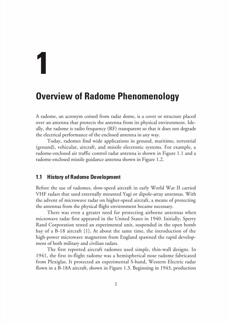
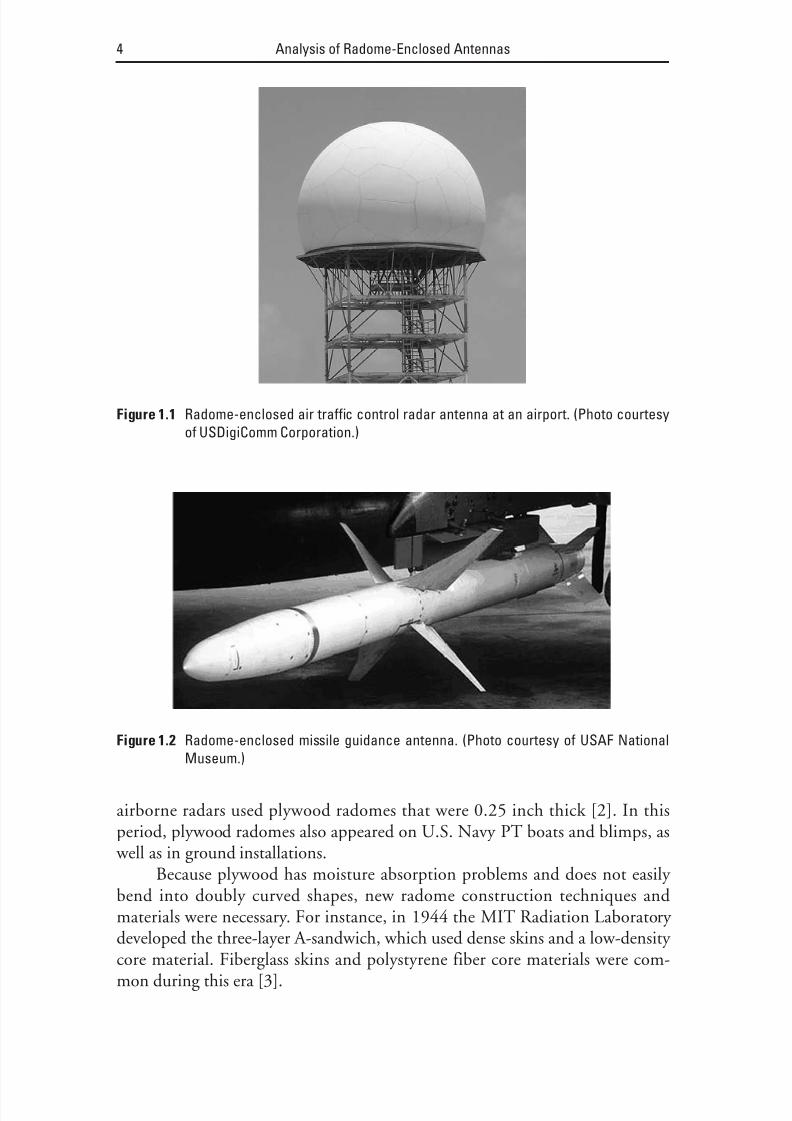
radome-enclosed air traffic control radar antenna is shown in Figure 1.1 and a radome-enclosed missile guidance antenna shown in Figure 1.2.
1.1 History of Radome Development
Before the use of radomes, slow-speed aircraft in early World War II carriedVHF radars that used externally mounted Yagi or dipole-array antennas. Withthe advent of microwave radar on higher-speed aircraft, a means of protecting the antennas from the physical flight environment became necessary.
There was even a greater need for protecting airborne antennas whenmicrowave radar first appeared in the United States in 1940. Initially, Sperry Rand Corporation tested an experimental unit, suspended in the open bombbay of a B-18 aircraft [1]. At about the same time, the introduction of thehigh-power microwave magnetron from England spawned the rapid develop-ment of both military and civilian radars.
The first reported aircraft radomes used simple, thin-wall designs. In
1941, the first in-flight radome was a hemispherical nose radome fabricatedfrom Plexiglas. It protected an experimental S-band, Western Electric radarflown in a B-18A aircraft, shown in Figure 1.3. Beginning in 1943, production
3
8/20/2019 Analysis of Radome-Enclosed Antennas
http://slidepdf.com/reader/full/analysis-of-radome-enclosed-antennas 25/319
airborne radars used plywood radomes that were 0.25 inch thick [2]. In thisperiod, plywood radomes also appeared on U.S. Navy PT boats and blimps, as
well as in ground installations.
Because plywood has moisture absorption problems and does not easily bend into doubly curved shapes, new radome construction techniques andmaterials were necessary. For instance, in 1944 the MIT Radiation Laboratory developed the three-layer A-sandwich, which used dense skins and a low-density core material. Fiberglass skins and polystyrene fiber core materials were com-mon during this era [3].
4 Analysis of Radome-Enclosed Antennas
Figure 1.1 Radome-enclosed air traffic control radar antenna at an airport. (Photo courtesy
of USDigiComm Corporation.)
Figure 1.2 Radome-enclosed missile guidance antenna. (Photo courtesy of USAF National
Museum.)

8/20/2019 Analysis of Radome-Enclosed Antennas
http://slidepdf.com/reader/full/analysis-of-radome-enclosed-antennas 26/319
However, since World War II, radome materials have continued todevelop in two main areas: ceramics, used primarily for hyper velocity missileradomes, and high-strength organic materials for sandwich composite radomes.
Today, the most modern of aircraft radomes use sandwich-wall construc-tion. Figure 1.4 shows a modern aircraft with a radar nose radome designed witha sandwich wall construction.
Advanced computerized design analysis techniques have also appeared asthe result of electronic performance requirements for new avionics and radars.The distribution of radome technology data through the various symposia is the
primary force advancing computerized design analysis techniques. The most well known of these symposia was probably the biennial Electromagnetic Win-dow Symposium held at the Georgia Institute of Technology in Atlanta,Georgia.
1.2 Radome-Antenna Interaction
Over recent decades, the rapid growth in the use of the electromagnetic spec-trum has led to many improvements in the performance of the antennas associ-ated with electromagnetic sensors or communications electronics. Twoexamples of these improvements are dual-polarized ultrawideband antenna sys-tems for improved radar performance and very low sidelobe antennas for use in
Overview of Radome Phenomenology 5
Figure 1.3 Photograph of a B-18A aircraft. (Photo courtesy of USDigiComm Corporation.)

8/20/2019 Analysis of Radome-Enclosed Antennas
http://slidepdf.com/reader/full/analysis-of-radome-enclosed-antennas 27/319
SATCOM communications equipment which must meet very stringent, far-outsidelobe requirements.
The antennas associated with these equipments require far more stringentradome performances than their predecessors because the antenna performancecan be altered by radome effects that include, but are not limited to:
1. Introduction of a boresight error (BSE) and boresight error slope(BSES);
2. Introduction of a registration error;
3. Increased antenna sidelobe levels;
4. Increased depolarization or the folding of energy from one polarizationsense to the other;
5. Increase in antenna voltage standing wave ratio (VSWR);
6. Introduction of an insertion loss due to the presence of the radome.
1.2.1 Boresight Error (BSE) and Boresight Error Slope (BSES)
BSE is a bending of the angle of arrival of a received signal relative to its actualangle of arrival or line of sight. This phenomenon stems primarily from distor-tions of the electromagnetic wavefront as it propagates through a dielectric
6 Analysis of Radome-Enclosed Antennas
Figure 1.4 Radome-enclosed radar antenna on the nose of a modern aircraft. (Photograph
courtesy of USAF National Museum.)

8/20/2019 Analysis of Radome-Enclosed Antennas
http://slidepdf.com/reader/full/analysis-of-radome-enclosed-antennas 28/319
radome wall. BSES is defined as the rate of change of BSE as a function of theantenna scan angle within the radome.
For a radome-enclosed missile monopulse antenna, BSE depends on fre-
quency, polarization, and antenna orientation. Radome BSE directly affects themiss distance of a missile flying a pursuit guidance trajectory. Radome BSESalso impacts the miss distance (or guidance accuracy) of a missile flying a pro-portional or modern guidance law trajectory [4].
Radome BSES can cause severe degradation for modern guidance systemsand classical proportional navigation systems. Missile guidance system designersoften use computer and/or hardware in-the-loop (HWIL) simulations to deter-mine the relationship between a missile terminal miss distance versus the BSESof the radome. The desired guidance accuracy will dictate a maximum allowable
BSES.In production, the radome manufacturing tolerance affects the BSES char-
acteristics of the radome. As a result of the computer and/or HWIL simulationsdiscussed earlier, the maximum allowable BSES is often used to specify therequired manufacturing tolerances of the radome [5].
1.2.2 Registration Error
Registration error is the difference in uplink frequency and downlink frequency BSE in the case of radome-enclosed SATCOM antennas. It is important thatthis parameter be sufficiently small to assure that both the transmit beam andreceive beam peaks are coaligned on the same satellite.
1.2.3 Antenna Sidelobe Degradation
Antenna sidelobes generally increase when an antenna is placed within a radome. This increase occurs because of distortion and wall transmission effects
as a wavefront propagates through a radome wall. The state of the art of low-sidelobe-level antennas has progressed to the point where the radome is themain source of clutter, resulting from increased sidelobes [6].
1.2.4 Depolarization
Radome depolarization is a folding of energy from the primary antenna polar-ization to the other sense. For instance, assume that the antenna is receiving a
right-hand circularly polarized (RHCP) signal. After the received signal propa-gates through the radome wall, part of the energy is converted into a left-handcircularly polarized (LHCP) signal. This phenomenon occurs as a result of theradome wall curvature and the difference in complex transmission coefficientbetween orthogonal polarized vectors.
Overview of Radome Phenomenology 7

8/20/2019 Analysis of Radome-Enclosed Antennas
http://slidepdf.com/reader/full/analysis-of-radome-enclosed-antennas 29/319
Depolarization can be a big problem, particularly with satellite communi-cations (SATCOM) ground terminals that utilize frequency reuse, such as thetypical SATCOM on a ship shown in Figure 1.5. Here two independent signals
are transmitted or received within the same frequency channel, but in oppositepolarization senses.
1.2.5 Antenna Voltage Standing Wave Ratio (VSWR)
The antenna VSWR can greatly increase from RF power reflected from theinner radome wall surface. The VSWR increase from this radome reflectedpower will represent an additional gain/loss that can be critical to, for example,
SATCOM communications systems.
1.2.6 Introduction of an Insertion Loss Due to the Presence of the Radome
Lastly, radome insertion loss is a reduction in signal strength as the electromag-netic wave propagates through the dielectric radome wall. Part of the loss occursas a reflection at the air/dielectric interface. The remainder of the loss occursfrom dissipation within the dielectric layers. The material loss tangent or tanδ is a
measure of these dissipative losses.
1.3 Significance of Parameters in Radome Performance
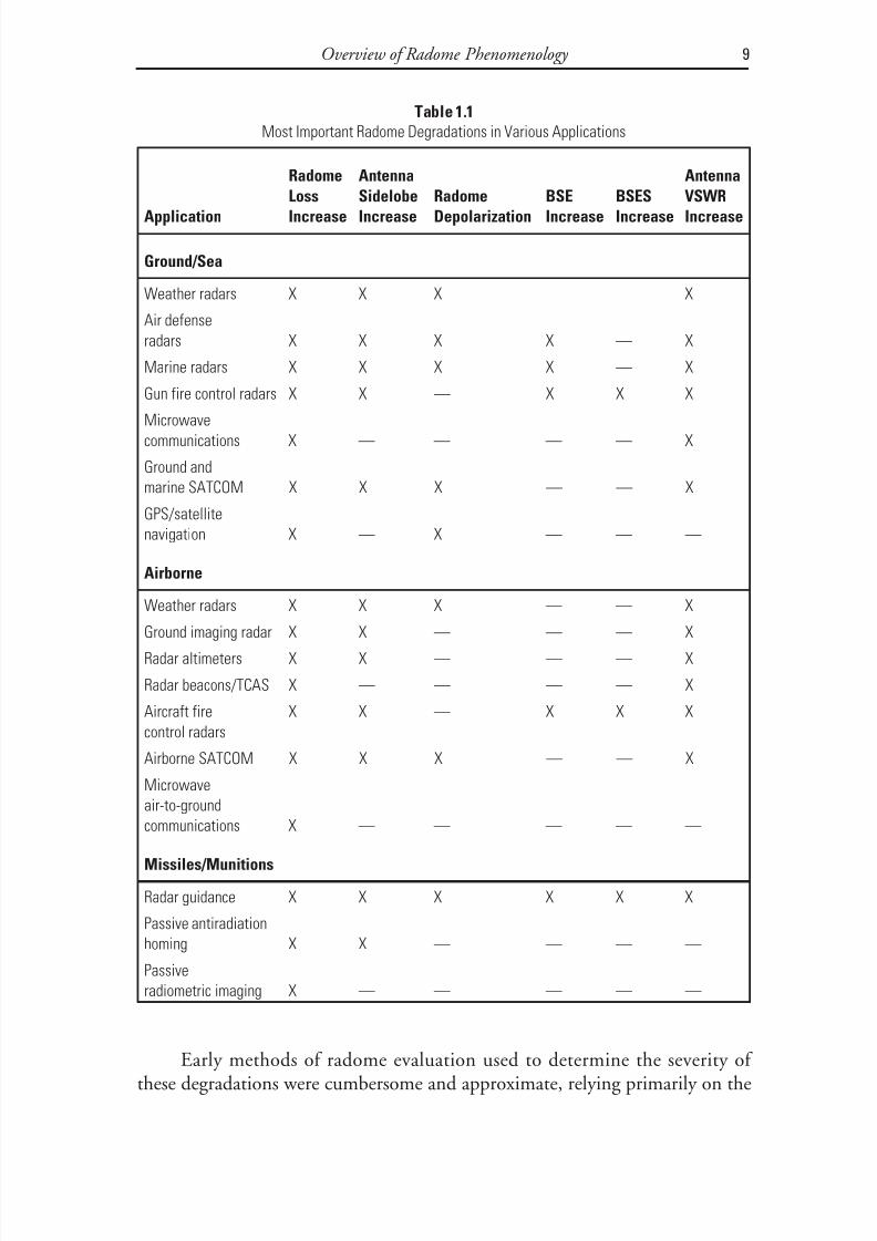
The particular application decides which radome-induced effects are of greatestconcern. Table 1.1 gives an overview of the most typical radome degradationsthat are most important to the design engineer in various sensor or electronics
applications.
8 Analysis of Radome-Enclosed Antennas
Figure 1.5 Radome-enclosed SATCOM antennas on a ship. (Photo courtesy of USDigiComm
Corporation.)
8/20/2019 Analysis of Radome-Enclosed Antennas
http://slidepdf.com/reader/full/analysis-of-radome-enclosed-antennas 30/319
Early methods of radome evaluation used to determine the severity of these degradations were cumbersome and approximate, relying primarily on the
Overview of Radome Phenomenology 9
Table 1.1
Most Important Radome Degradations in Various Applications
Application
Radome
LossIncrease
Antenna
SidelobeIncrease
RadomeDepolarization
BSEIncrease
BSESIncrease
Antenna
VSWRIncrease
Ground/Sea
Weather radars X X X X
Air defense
radars X X X X — X
Marine radars X X X X — X
Gun fire control radars X X — X X X
Microwave
communications X — — — — X
Ground and
marine SATCOM X X X — — X
GPS/satellite
navigation X — X — — —
Airborne
Weather radars X X X — — X
Ground imaging radar X X — — — X
Radar altimeters X X — — — X
Radar beacons/TCAS X — — — — X
Aircraft fire
control radars
X X — X X X
Airborne SATCOM X X X — — X
Microwaveair-to-ground
communications X — — — — —
Missiles/Munitions
Radar guidance X X X X X X
Passive antiradiation
homing X X — — — —
Passiveradiometric imaging X — — — — —

8/20/2019 Analysis of Radome-Enclosed Antennas
http://slidepdf.com/reader/full/analysis-of-radome-enclosed-antennas 31/319
use of the nomograph [7]. With the arrival of the computer, modern mathemat-ical approaches began to appear, featuring better computational accuracy [8].
For high-accuracy radome performance computations, the efficiency of
the calculation determines its limitation as a design tool. Therefore, the combi-nation of accuracy and efficiency must be a goal in any radome-antenna analysisapproach.
In addition, the radome design community faces increased computer runtimes for analysis of new millimeter wave (very short wavelength) radar systems.The increased run time is due to the fact that sample spacings are typically a half
wavelength over the antenna aperture in order to avoid computational errorsthat occur when grating lobes come into real space. This additional run timeadds impetus to the search for more efficient methods of performing millime-
ter-wave radome analysis.Fortunately, computational approaches that would have required a main-
frame a few years ago can now utilize the low-cost, high-performance personalcomputer (PC). The goal of this book is to provide you with working tools ame-nable to PC modeling so that you can quantify the radome-induced parametersof interest in a particular application.
1.4 Radome Technology Advances Since the First Edition
Since the first edition of this book, the greatest advances in radome technology probably have been in the use of metamaterials or frequency selective layers
within the radome wall composite. A brief discussion of these advances appearsin the following.
1.4.1 Use of Metamaterials
Metamaterials are unique materials possessing characteristics opposite to thoseof naturally occurring materials. They exhibit unusual electrical properties suchas a reversal of Snell’s law. A metamaterial is a material that gains its propertiesfrom its structure rather than directly from its composition. The term wascoined in 1999 by Rodger M. Walser of the University of Texas at Austin [9],
who defined metamaterials as macroscopic composites having a manmade,three-dimensional, periodic cellular architecture designed to produce an opti-
mized combination not available in nature. In simple terms, it is a manmadecomposite material that exhibits a negative index of refraction. Additionalinformation about metamaterials appears in [10].
The design of an antenna radome using such metamaterials can enhanceantenna gain. Research by Liu et al. [11] used multilayered structures composedof two materials with left-handed materials having an average index of refraction
10 Analysis of Radome-Enclosed Antennas

8/20/2019 Analysis of Radome-Enclosed Antennas
http://slidepdf.com/reader/full/analysis-of-radome-enclosed-antennas 32/319
close to zero and air. Liu et al.’s analysis showed a beamwidth reduction of 37.5% and an antenna gain increase of about 6 dBi.
Work by Metz [12] used metamaterials to create a biconcave lens architec-
ture for focusing the microwaves transmitted by the antenna, in which thesidelobes of the antenna were greatly reduced. This suggests that such materialsmay have a role in minimizing the effects of sidelobe degradation, which is very important to radome-enclosed SATCOM antennas.
Metamaterials have also been used to compensate for the effects of radomeBSE [13]. In one compensation technique comprised of a two-layer radome, aninner metamaterial layer of a negative index of refraction material is used withan outer layer of a conventional radome dielectric material having a positiveindex of refraction material. The thickness of the two materials and their respec-
tive refractive indices are adjusted so that a beam of electromagnetic energy pass-ing through the radome is effectively not refracted.
1.4.2 Frequency Selective Radomes
Under many circumstances it is desirable to add frequency selectivity to a radome to prevent coupling from nearby transmit antennas that may interfere
with the electronics. For instance, a radome-enclosed IRIDIUM antenna receiv-
ing relatively weak satellite signals may be interfered with by a high-power trans-mitter on the same platform. What might be employed is a frequency selectivesurface on the IRIDIUM radome providing a bandpass performance at theIRIDIUM frequency, and/or a band reject frequency selective surface on theIRIDIUM radome providing a band reject performance at the interfering trans-mit frequency that may be overloading the IRIDIUM receiver.
The frequency selective surface (FSS) layer is generally arranged on thesurface of the radome wall composite, and a discussion of design techniquesappear in [14–17]. However, there is no reason why the FSS layer cannot bearranged on the inner surface of the radome wall composite or even embedded
within the wall. FSS surfaces usually consist of arrays of etched antenna elementsof some kind and can be designed to either reflect or transmit electromagnetic
waves with a frequency discrimination. The simplest of these are conducting strips (or conducting slots in a metal ground plane), which can be represented incomputer modeling by reactive equivalent components. Reactive componentscan also be identified in other, more complicated elements such as square loopsor slots and Jerusalem cross geometries. For FSS band transmission behavior,
these elements mostly take the form of slot geometries in a conducting radome wall layer.
For a monolithic wall radome, Purinton [18] has investigated the possibil-ity of embedding a wire mesh or screen into the radome material itself. Theinductance can be arranged to offset the capacitance of the radome dielectric
Overview of Radome Phenomenology 11

8/20/2019 Analysis of Radome-Enclosed Antennas
http://slidepdf.com/reader/full/analysis-of-radome-enclosed-antennas 33/319
material. By proper design, a radome can be built that will pass only a singleband of frequencies centered on any desired operating radar frequency. Wu [19]has developed an approach to obtain a multiple bandpass FSS performance.
1.4.3 Concealed Radomes
Zoning regulations, land developer/subdivision covenants, and other legalrestrictions have sometimes created problems for telecom companies installing sensitive microwave and SATCOM antennas of various types within certain
12 Analysis of Radome-Enclosed Antennas
(b)
(a)
Figure 1.6 (a, b) Microwave antenna within an RF transparent structure. (Photo courtesy of
ConcealFab Corporation.)

8/20/2019 Analysis of Radome-Enclosed Antennas
http://slidepdf.com/reader/full/analysis-of-radome-enclosed-antennas 34/319
urban areas. Unique cost-effective RF transparent structures have been recently designed and engineered out of innovative structural shapes and constructedfrom plastic materials that will last a lifetime [20]. These structures are light-
weight and blend into virtually any environment and can be fabricated to resem-ble virtually any building configuration, as shown in Figure 1.6, which encloses
a small microwave antenna. The concept is scalable to any antenna size as illus-trated for a very large antenna in Figure 1.7.
References
[1] Tice, T. E., “Techniques for Airborne Radome Design,” AFATL-TR-66-391, Air Force Avionics Laboratory, AFSC, Wright Patterson AFB, Ohio, December 1966.
[2] Baxter, J. P., Scientists Against Time , Boston, MA: Little, Brown and Company, 1952.
[3] Eggleston, W., Scientists at War , Toronto, Canada: Hunter Rose Company, Ltd., 1950.
[4] Johnson, R. C., “Seeker Antennas,” Ch. 38 in Antenna Engineering Handbook , 3rd ed.,New York: McGraw-Hill, 1992.
Overview of Radome Phenomenology 13
Figure 1.7 Very large microwave antenna within an RF transparent structure. (Photo cour- tesy of ConcealFab Corporation.)
8/20/2019 Analysis of Radome-Enclosed Antennas
http://slidepdf.com/reader/full/analysis-of-radome-enclosed-antennas 35/319
[5] Yueh, W. R., “Adaptive Estimation Scheme of Radome Error Calibration,” Proceedings of the 22nd IEEE Conference on Decision and Control , Vol. 8, No. 5, 1983, pp. 666–669.
[6] Rulf, B., “Problems of Radome Design for Modern Airborne Radar,” Microwave Journal ,Vol. 28, No. 5, May 1995, pp. 265–271.
[7] Kaplun, V. A., “Nomograms for Determining the Parameters of Plane Dielectric Layers of Various Structure with Optimum Radio Characteristics,” Radiotechnika I Electronika (Russian), Part 2, Vol. 20, No. 9, 1965, pp. 81–88.
[8] Bagby, J., “Desktop Computer Aided Design of Aircraft Radomes,” IEEE MIDCON 1988 Conference Record , Western Periodicals Company, N. Hollywood, CA, 1988, pp.258–261.
[9] Walser, R. M., Introduction to Complex Mediums for Electromagnetics and Optics, W. S. Weiglhofer and A. Lakhtakia, (eds.), Bellingham, WA: SPIE Press, 2003.
[10] Smith, D. R., et al, “Composite Medium with Simultaneously Negative Permeability andPermittivity,” Physical Review Letters , Vol. 84, No. 18, May 2000.
[11] Liu, H. -N., et al., “Design of Antenna Radome Composed of Metamaterials for HighGain,” IEEE Antennas and Propagation Society International Symposium 2006 , July 9–14,2006, pp. 19–22.
[12] Metz, C., “Phased Array Metamaterial Antenna System,” U.S. Patent, October 2005,http://patft.uspto.gov/netacgi/nph-Parser?Sect2=PTO1&Sect2=HITOFF&p=1&u=%2Fnetahtml%2FPTO%2Fsearch-bool.html&r=1&f=G&l=50&d=PALL&RefSrch=yes&Qu
ery=PN%2F6958729-h0#h0http://patft.uspto.gov/netacgi/nph-Parser?Sect2=PTO1&Sect2=HITOFF&p=1&u=%2Fnetahtml%2FPTO%2Fsearch-bool.html&r=1&f=G&l=50&d=PALL&RefSrch=yes&Query=PN%2F6958729-h2#h26,958,729.
[13] Schultz, S. M., D. L. Barker, and H. A. Schmitt, “Radome Compensation Using MatchedNegative Index or Refraction Materials,” U.S. Patent 6,788,273, September 2004.
[14] Parker, E. A., “The Gentleman’s Guide to Frequency Selective Surfaces,” 17th Q.M.W. Antenna Symposium , London, Electronic Engineering Laboratories, University of Kent, April 1991
[15] Munk, B. A., Frequency Selective Surfaces , New York: John Wiley & Sons, 2000.
[16] Vardaxoglou, J. C., Frequency Selective Surface: Analysis and Design , Electronic & ElectricalEngineering Series, Taunton, Somerset, England: Research Studies Press, 1997.
[17] Wang, Z. L., et al., “Frequency-Selective Surface for Microwave Power Transmission,”IEEE Transactions on Microwave Theory and Techniques , Vol. 47, No. 10, October 1999,pp. 2039–2042.
[18] Purinton, D. L., “Radome Wire Grid Having Low Pass Frequency Characteristics,” U.S.Patent 3,961,333, 1976.
[19] Wu, T. -K., “Multi-Band Frequency Selective Surface with Double-Square-Loop PatchElements,” Jet Propulsion Laboratory, NTRS: 2006-12-25, Document ID: 20060037676,available through National Technology Transfer Center (NTTC), Wheeling, WV, 1995.
[20] http://www.concealfab.com.
14 Analysis of Radome-Enclosed Antennas

8/20/2019 Analysis of Radome-Enclosed Antennas
http://slidepdf.com/reader/full/analysis-of-radome-enclosed-antennas 36/319
2Basic Principles and Conventions
This chapter provides a reference and review of topics used in the modeling of radome-covered antennas. The topics covered in this chapter are:
• Vector mathematics;
• Electromagnetic theory;
• Matrices;
• Coordinate systems and antenna pointing gimbals.
These topics are not treated rigorously, but rather in a top-level summary.If you are well versed in these subjects, you may wish to skip most of this chap-ter. However, you should review Section 2.4, which defines reference conven-tions used in later mathematical modeling.
2.1 Vector Mathematics
A Cartesian coordinate system is used where a vector is represented as the sumof three vectors parallel to Cartesian coordinate axes, with the components of given by a x , a y , a z . For this purpose, we associate with that coordinate systemthree mutually perpendicular unit vectors ( , , )x y z , which have the positivedirections of the three-coordinate axes. Accordingly, the vector can be repre-sented as
A a x a y a z x y z = + + (2.1)
15

8/20/2019 Analysis of Radome-Enclosed Antennas
http://slidepdf.com/reader/full/analysis-of-radome-enclosed-antennas 37/319
Figure 2.1 illustrates the three unit vectors x y z , , when the origin is cho-sen as their common initial point and vector A in this coordinate system. In a like manner, another vector may be defined as
B b x b y b z x y z (2.2)
The dot and scalar cross products of vectors A and B are both scalar quan-tities expressed in terms of the angle ψ between the two vectors [1].
A B AB ⋅ cos ψ (2.3)
A B AB × = sin ψ (2.4)
where the magnitude of these two vectors are expressed by the following twoformulas:
A a a a x y z = + +2 2 2 (2.5)
B b b b x y z 2 2 2
(2.6)
However, the vector cross product of vectors A and B results in anothervector, which can be defined as:
C A B (2.7)
This is illustrated in Figure 2.2.
16 Analysis of Radome-Enclosed Antennas
(a) (b)
Figure 2.1 (a) The unit vectors x y z , , and (b) representation of vector A .

8/20/2019 Analysis of Radome-Enclosed Antennas
http://slidepdf.com/reader/full/analysis-of-radome-enclosed-antennas 38/319
This vector is orthogonal to the plane in which vectors A and B lie, and itssense is determined by the right-hand rule. In a matrix form, it is given by [2]:
C x y z
a a a
b b b x y z
x y z
(2.8)
or, expanding the matrix
( ) ( ) ( )C a b b a x a b b a y a b b a z y z y z z x z x x y x y = − + − + − (2.9)
Other vector manipulations that are worth mentioning include thefollowing:
• The distributive law for scalar multiplication [3]:
( ) A B C A B A C ⋅ = ⋅ + ⋅ (2.10)
• The distributive law for vector multiplication:
( ) A B C A B A C × = × + × (2.11)
• The scalar and vector triple products, respectively:
( ) ( ) ( ) ( ) A B C A B C C A B B C A ⋅ × = × ⋅ ⋅ + ⋅ × (2.12)
( ) ( ) ( ) A B C A C B A B C × × = ⋅ − ⋅ (2.13)
Finally, some relationships important in electromagnetic theory are asfollows:
Basic Principles and Conventions 17
Figure 2.2 Dot and cross products of vectors A and B .
8/20/2019 Analysis of Radome-Enclosed Antennas
http://slidepdf.com/reader/full/analysis-of-radome-enclosed-antennas 39/319

8/20/2019 Analysis of Radome-Enclosed Antennas
http://slidepdf.com/reader/full/analysis-of-radome-enclosed-antennas 40/319
D E ε (2.22)
The preceding differential equations are the fundamental Maxwell rela-
tionships, written in a rationalized meter, kilogram, seconds (mks) system of units. In this system, we have
E = electric intensity (V/m);
D = electric displacement (C/m2);
H = magnetic intensity (A/m);
B = magnetic induction (Wb/m);
µ = µr µo = permeability or magnetic inductive capacity of medium
(H/m); µr = relative permeability (dimensionless);
µo = 4 π × 10−7 = 1.257 × 10⁻⁶ H/m;
ε = permittivity or electric inductive capacity of medium (F/m);
εr = relative permittivity or relative dielectric constant (dimensionless);
εo = 8.854 × 10⁻¹²
F/m.
Note that the permittivity is a complex number:
ε ε ε j (2.23)
where ε′ is the real part of ε in farads per meter and ε″ is the imaginary part of εalso in farads per meter.
Assuming a time harmonic field of the form e jwt , a solution is required forthe wave equation developed from Maxwell’s equations
∇2 2
E k E (2.24)
A solution to this differential equation for a wave propagating in thez -direction takes the form e − jkt , where k is the wave number. The wave number iscomplex for waves propagating through a typical dielectric radome material:
jk j j j j
ω µ ε ε ω ωε
ε
ε( ) 1
(2.25)
In (2.25), it is convenient to introduce the concept of a dielectric materialloss tangent:
Basic Principles and Conventions 19

8/20/2019 Analysis of Radome-Enclosed Antennas
http://slidepdf.com/reader/full/analysis-of-radome-enclosed-antennas 41/319
tan δ ε
ε
(2.26)
This concept allows the wave number to be broken into real and imagi-nary parts [4]:
[ ] α ω µε
δ
2
1 12(tan ) (2.27)
[ ] β ω ωε
δ
2
1 12(tan ) (2.28)
Using this notation, the wave propagating through the dielectric in thez-direction then takes the more convenient form:
E E e E e e o jkz
o z j z α β− (2.29)
In this equation, α is known as the attenuation constant and β is known asthe phase constant. An electromagnetic wave is then both attenuated and phase
shifted as it propagates through a dielectric medium.For a wave propagating in the z-direction, valid solutions to the wave
equation are orthogonal signal sets E x , H y or E y , H x , which are related by the wave impedance of the medium:
E
H
E
H x
y
y
x
= = η (2.30)
In terms of the definition of polarization of the wave, note the following:
• The polarization is linear when only E x or E y exists or when both com-ponents exist simultaneously but are in phase.
• The polarization is elliptical when two components exist, are unequal inamplitude, and are out of phase with each other.
• The polarization is said to be circular when two components exist and
are equal in amplitude and the phase is a +90° or −90° difference.
Because of the modeling used in later sections of this book, an electromag-netic wave incident on a dielectric medium must be quantified into twoorthogonal components. These components are defined as parallel and
20 Analysis of Radome-Enclosed Antennas

8/20/2019 Analysis of Radome-Enclosed Antennas
http://slidepdf.com/reader/full/analysis-of-radome-enclosed-antennas 42/319
perpendicular to the plane formed by a vector in the direction of propagationand a vector normal to the surface of the radome at the incidence point.
The convention used for parallel and perpendicular wave components for
a wave propagating from free space and an incident on a dielectric medium isillustrated in Figure 2.3.
2.3 Matrices
Matrix algebra is a powerful mathematical tool in connection with linear equa-tions and transformations [5].
An m × n matrix is an ordered set of mn quantities, arranged in a rectan-
gular array of m rows and n columns. If m = n, the array is a square matrix of order n. A matrix having only one column is called a column matrix or column vector .
The following are useful relationships for m × n matrices [F ], [G ], [ J ], andarbitrary constants u and v :
[ ] [ ] [ ] [ ]F G G F + = + (2.31)
[ ]( ) ( )[ ]u v F uv F = (2.32)
Basic Principles and Conventions 21
Figure 2.3 Illustration of parallel and perpendicular wave components.

8/20/2019 Analysis of Radome-Enclosed Antennas
http://slidepdf.com/reader/full/analysis-of-radome-enclosed-antennas 43/319
( )[ ] [ ] [ ]u v F u F v F + = + (2.33)
[ ] [ ] [ ]( ) [ ] [ ] [ ]( )F G J F G J + + = + + (2.34)
[ ] [ ]( ) [ ] [ ]u F G u F u G + = + (2.35)
If we have an m × n matrix [G ] and an n × p matrix [ J ], the product of [G ]and [ J ] is an m × p matrix given by
[ ] [ ][ ]F G J = (2.36)
We can only multiply two matrices if the number of columns of the firstfactor is equal to the number of rows in the second.
The set of relations given in (2.36) can be solved for [ J ] via Cramer’s rule[6] in order to obtain an inverse transformation
[ ] [ ][ ] [ ] [ ] [ ]G G J J G F − −= =1 1
(2.37)
where the identity matrix is defined via
[ ] [ ] [ ]I G G = −1(2.38)
We will now demonstrate the inverse transformation. Consider [G ] repre-sented by:
[ ]G
g g g
g g g
g g g
=
11 12 13
21 22 23
31 32 33
(2.39)
The first step in the process is to form the transpose of [G ]
[ ]G
g g g
g g g
g g g
T =
11 21 31
12 22 32
13 23 33
(2.40)
22 Analysis of Radome-Enclosed Antennas

8/20/2019 Analysis of Radome-Enclosed Antennas
http://slidepdf.com/reader/full/analysis-of-radome-enclosed-antennas 44/319

8/20/2019 Analysis of Radome-Enclosed Antennas
http://slidepdf.com/reader/full/analysis-of-radome-enclosed-antennas 45/319
• With a Cartesian coordinate system placed at the antenna center, com-pute the transformation that results from angular rotations.
• Transform results to a Cartesian coordinate system placed at center of a gimbal rotation, taking into account the rotational offsets.
• Linearly transform the results to true radome coordinates with the coor-dinate system located at the base of the radome.
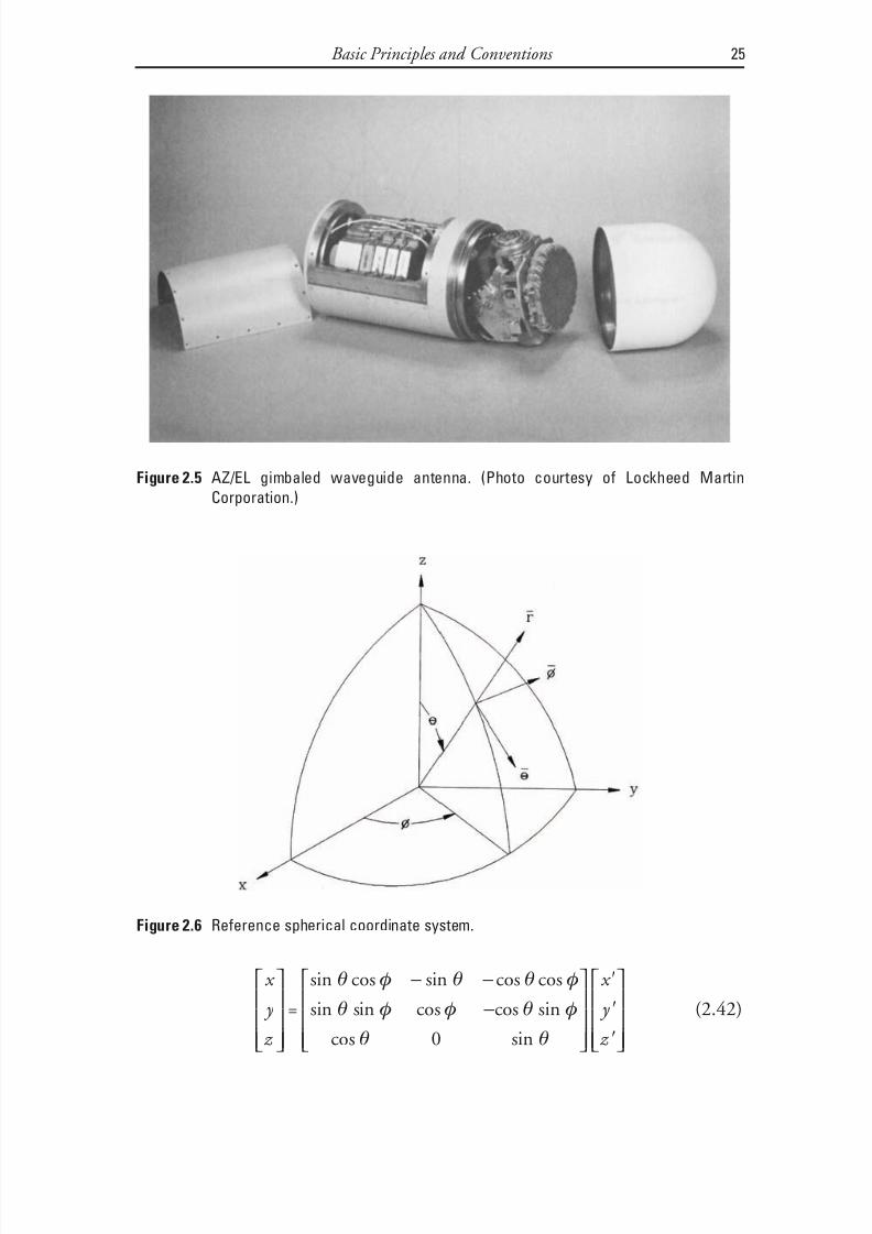
Consider the following development. With a coordinate system placed atthe antenna center, as illustrated in Figure 2.6, the transformation of any pointon the antenna aperture P a (x ′, y ′, z ′) is:
24 Analysis of Radome-Enclosed Antennas
Figure 2.4 (a) EL/AZ gimbal and (b) AZ/EL gimbal.
8/20/2019 Analysis of Radome-Enclosed Antennas
http://slidepdf.com/reader/full/analysis-of-radome-enclosed-antennas 46/319
x
y
z
=
− −−
sin cos sin cos cos
sin sin cos
θ φ θ θ φ
θ φ φ cos θ φ
θ θ
sin
cos sin0
x
y
z
(2.42)
Basic Principles and Conventions 25
Figure 2.5 AZ/EL gimbaled waveguide antenna. (Photo courtesy of Lockheed Martin
Corporation.)
Figure 2.6 Reference spherical coordinate system.

8/20/2019 Analysis of Radome-Enclosed Antennas
http://slidepdf.com/reader/full/analysis-of-radome-enclosed-antennas 47/319
If we let ψ = 90° − θ, then this becomes
x
y z
=
− −
−
cos cos sin sin cos
cos sin cos
ψ φ φ ψ φ
ψ φ φ sin ψ φ ψ ψ
sinsin cos0
x
y z
(2.43)
The coordinate system space is illustrated in Figure 2.7 for the elevationover azimuth (EL/AZ) antenna gimbal case and illustrated in Figure 2.8 for theazimuth over elevation (AZ/EL) antenna gimbal case.
For the EL/AZ antenna gimbal case, we can now incorporate translationsdue to the offsets from the gimbal point. We do this by first applying the eleva-
tion gimbal rotation with x ′ = ∆b , ψ = 0 and φ = EL . Next, the azimuth offset,∆a , and then the azimuth gimbal rotation is applied by letting φ = 0 and ψ = AZ .
We then obtain for the transformation [personal communication with RichMatyskiela, AEL Industries, Lansdale, Pennsylvania, 1994]:
26 Analysis of Radome-Enclosed Antennas
Figure 2.7 EL/AZ coordinate system.

8/20/2019 Analysis of Radome-Enclosed Antennas
http://slidepdf.com/reader/full/analysis-of-radome-enclosed-antennas 48/319
x
y
z
AZ AZ
AZ AZ
=−
cos sin
sin cos
0
0 1 0
0
−
EL EL
EL EL b cos sin
sin cos
0
0
0 0 1
∆′′
+
y
z
a ∆0
0
(2.44)
Performing the indicated matrix multiplications, and adding a translation
for the initial gimbal location P g (x g , 0, 0), we obtain the final result:
x
y
z
AZ EL AZ EL A
=− −cos cos cos sin sin Z
EL EL
AZ EL AZ EL AZ
sin cos
sin cos sin sin cos
0
−
′′
+
y
z
AZ
AZ
b
a
a
∆
∆
∆
cos
sin
0
+
x g
0
0
(2.45)
Similarly, for an AZ/EL gimbal, the matrix solution in (2.46) includes thesame translations for the rotational offsets and the initial gimbal location:
Basic Principles and Conventions 27
Figure 2.8 AZ/EL coordinate system.

8/20/2019 Analysis of Radome-Enclosed Antennas
http://slidepdf.com/reader/full/analysis-of-radome-enclosed-antennas 49/319
x
y
z
EL AZ EL EL A
=− −cos cos sin cos sin Z
EL AZ EL EL AZ
AZ AZ
sin cos cos sin sin
sin cos
−
0
′′
+
y
z
EL
EL
b
a
a
∆
∆∆
cos
sin
0
+
x g
0
0
(2.46)
In computer modeling of radome-enclosed gimbaled antenna cases dis-cussed later in this book, we will use these latter two expressions extensively.
2.5 Specialized Antenna Pointing Gimbals
We consider gimbals in radome analysis for the mathematical transformationbetween the commanded antenna azimuth (AZ) and elevation (EL) angle point-ing and the coordinates of rotated points on the antenna aperture.
Gimbal mountings for antennas have been made in many different config-urations such as Figure 2.9. For dynamic situations that require the motion of
the platform on which the radome enclosed antenna is mounted to be isolatedfrom the antenna pointing gimbal within the radome, the easiest and moststraightforward approach is to provide a separate set of gimbals to isolate thestandard EL/AZ or AZ/EL antenna gimbals within the radome from the plat-form motion [7].
For rapid platform directional changes, it is important that the accuracy,stability, and stiffness of the positioner be acceptable under worst-case dynamic
28 Analysis of Radome-Enclosed Antennas
Figure 2.9 Specialized antenna gimbal that is neither AZ/EL or EL/AZ. (Photo courtesy of K.
Guerin and E. Bannon of Carnegie Mellon University.)

8/20/2019 Analysis of Radome-Enclosed Antennas
http://slidepdf.com/reader/full/analysis-of-radome-enclosed-antennas 50/319
and environmental conditions. The positioning accuracy is determined by how precisely the positioner can move to a defined point as well as how stable andstiff the positioner is in maintaining that position. The speed of movement is
based on how quickly the positioner can move from one angular position toanother.Numerous more sophisticated gimbal approaches have been developed to
combine antenna pointing and platform isolation within a single device. Forinstance, in a patent, Speicher describes a gimbal assembly in which the outergimbal member is an arcuate yoke mounted on rollers to rotate about one axisand the inner gimbal member is a platform pivotally mounted in the yoke torotate about a second orthogonal axis. Two motors are connected through a dif-ferential drive system to rotate either gimbal member selectively or both together
in any combination of motions [8].In a patent by Vucevic [9] a stabilized platform that is suitable for stabiliz-
ing the boresight of a communications antenna is provided with a pendulousmounting that holds the structure erect. A pair of gyroscopes gives active controlof the attitude of the platform and is coupled to the platform via a gear arrange-ment. When the platform is rotated rapidly (to unravel feed cables or to permitoverhead tracking of the antenna), the gyroscopes experience a much lesserdegree of movement that is determined by the gearing ratio, so that the
gyroscopes are not destabilized.Many other approaches are possible [10–12]. In the following sections we
consider three cases in which specialized antenna pointing gimbals may berequired: marine SATCOM, vehicular SATCOM, and airborne applications.
2.5.1 Maritime SATCOM
In previous years shipboard satellite communications (SATCOM) systems werelimited to only C-band terminals for the transfer of high-speed data and mostused circularly polarized satellite transponders. In some instances the satellitelink used a linear transponder, but the terminal operator was then required tolease both polarizations, which essentially doubled the cost of the bandwidthbeing leased [13]. Currently, Inmarsat and mini-VSAT are two state-of-the-artservices for maritime communications. A disadvantage of VSAT is the require-ment for stabilized antenna systems because VSAT communications often oper-ate at Ku-bands in contrast to the low-frequency L-band used by Inmarsat.Because the beam is much narrower at this frequency band, it is even more
important to keep the antenna locked closely onto the satellite signal consider-ing the dynamic roll, pitch, and yaw motion of the vessel.
Loss in the gain in the use of marine SATCOM antennas is due to bothpointing errors and polarization misalignment. Many of the current generationof ship terminals use EL/AZ-type pedestals that require specialized design to get
Basic Principles and Conventions 29
8/20/2019 Analysis of Radome-Enclosed Antennas
http://slidepdf.com/reader/full/analysis-of-radome-enclosed-antennas 51/319
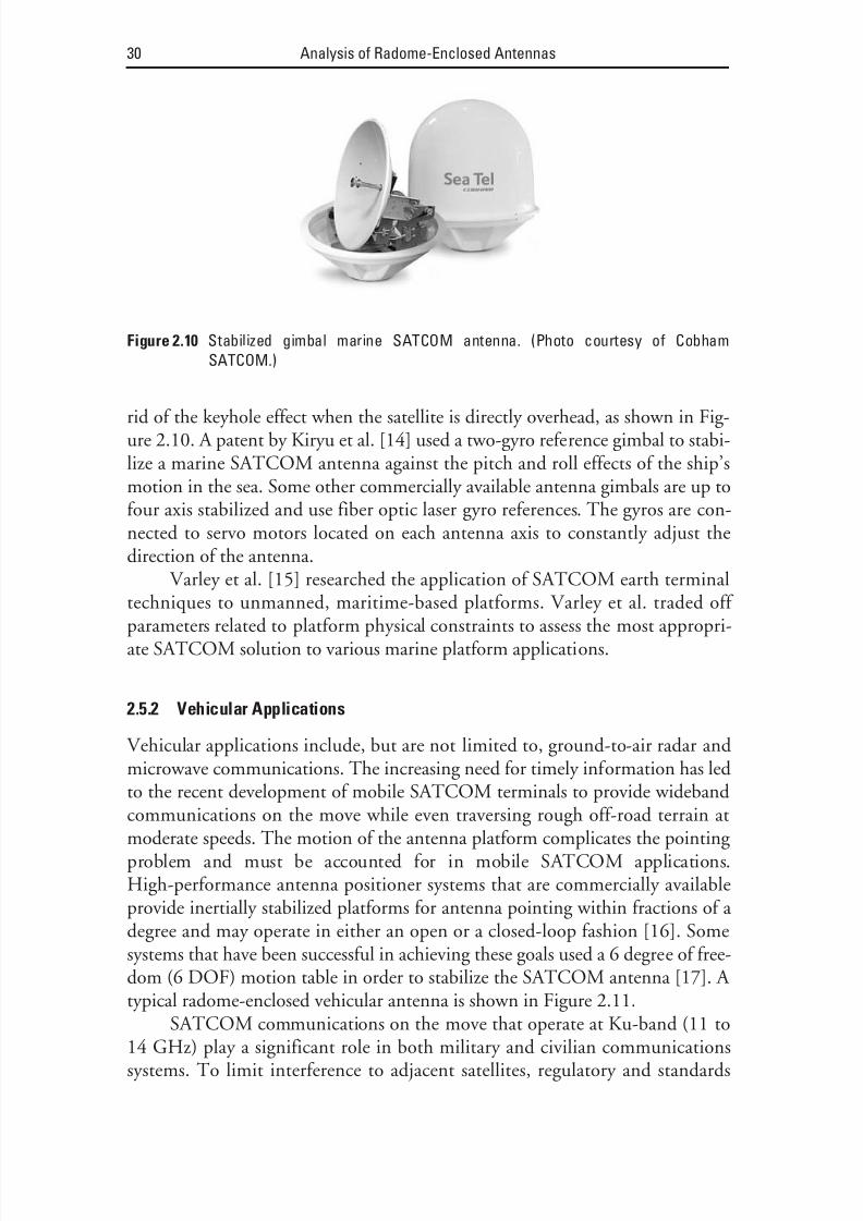
rid of the keyhole effect when the satellite is directly overhead, as shown in Fig-ure 2.10. A patent by Kiryu et al. [14] used a two-gyro reference gimbal to stabi-lize a marine SATCOM antenna against the pitch and roll effects of the ship’smotion in the sea. Some other commercially available antenna gimbals are up tofour axis stabilized and use fiber optic laser gyro references. The gyros are con-nected to servo motors located on each antenna axis to constantly adjust thedirection of the antenna.
Varley et al. [15] researched the application of SATCOM earth terminaltechniques to unmanned, maritime-based platforms. Varley et al. traded off parameters related to platform physical constraints to assess the most appropri-ate SATCOM solution to various marine platform applications.
2.5.2 Vehicular Applications
Vehicular applications include, but are not limited to, ground-to-air radar and
microwave communications. The increasing need for timely information has ledto the recent development of mobile SATCOM terminals to provide widebandcommunications on the move while even traversing rough off-road terrain atmoderate speeds. The motion of the antenna platform complicates the pointing problem and must be accounted for in mobile SATCOM applications.High-performance antenna positioner systems that are commercially availableprovide inertially stabilized platforms for antenna pointing within fractions of a degree and may operate in either an open or a closed-loop fashion [16]. Some
systems that have been successful in achieving these goals used a 6 degree of free-dom (6 DOF) motion table in order to stabilize the SATCOM antenna [17]. A typical radome-enclosed vehicular antenna is shown in Figure 2.11.
SATCOM communications on the move that operate at Ku-band (11 to14 GHz) play a significant role in both military and civilian communicationssystems. To limit interference to adjacent satellites, regulatory and standards
30 Analysis of Radome-Enclosed Antennas
Figure 2.10 Stabilized gimbal marine SATCOM antenna. (Photo courtesy of Cobham
SATCOM.)

8/20/2019 Analysis of Radome-Enclosed Antennas
http://slidepdf.com/reader/full/analysis-of-radome-enclosed-antennas 52/319
bodies have established strict limits on the effective isotropic radiated power(EIRP) in the antenna off-axis direction [18]. Vehicular SATCOM systems thatoperate at millimeter-wave frequencies are even more difficult to keep pointedtoward the satellite because of much narrower antenna beamwidths. One possi-bility is to use closed loop auto acquisition and tracking to keep the antenna pointed under dynamic conditions. However, a consequence of using auto track gimbals on a moving vehicle is that the registration error (the difference between
the transmit and receive frequency band BSE) must be suitably close so thatboth the peaks of the transmit and receive antenna beams are coaligned on thesame satellite. To achieve this, the stiffness and stability of the positioner mustbe suitable for extreme environmental conditions.
2.5.3 Airborne Applications
Airborne applications include, but are not limited to, SATCOM and
air-to-ground microwave communications. In a patent by Holandsworth andCantrell [19] the line of sight of an airborne radar antenna is stabilized from thepitch and roll motions of the aircraft by mounting the antenna on a three degreeof freedom gimbal system. The gimbal system is comprised of a first gimbalmounted for rotation about the aircraft Z -axis (azimuth) for pointing theantenna along the intended line of sight, a second gimbal mounted on the firstgimbal for rotating up and down with respect to the azimuth gimbal, and a thirdgimbal mounted on the second gimbal to which the antenna is connected toprovide rotation to align antenna polarization relative to inertial ground.
Pointing and scanning control algorithms for a two-axis gimbal, inertially stabilized, airborne antenna system are described in [20]. Satisfactory perfor-mance is demonstrated in the presence of aircraft maneuvers, with some(expected) degradation for the very-near-zenith antenna states. The antenna scanning algorithm presented is adaptive in its scan rate (to avoid scan
Basic Principles and Conventions 31
Figure 2.11 Vehicular radome-enclosed antenna. (Photo courtesy of USDigiComm
Corporation.)

8/20/2019 Analysis of Radome-Enclosed Antennas
http://slidepdf.com/reader/full/analysis-of-radome-enclosed-antennas 53/319
distortions due to the azimuth rate limiting imposed by the physical antenna system), is simple to implement, and properly accounts for aircraft maneuvering to maintain circular scanning trajectories in inertial space.
In a U.S. Army report a pedestal and gimbal assembly related to missilesemiactive radar seekers supported three gyroscopes and functions as a referenceplatform to relate airframe attitude. This is mechanized by utilizing the 2 degreeof freedom gimbal for pitch and yaw and controlling the missile body roll axisfor the third degree of freedom. Structure of the positioning system includes a pedestal having an inner gimbal assembly with a support for mounting theantenna assembly and the gyros. A yaw torque motor assembly is carried by theinner gimbal and is provided with a pair of output shafts for supporting theinner gimbal and controlling the yaw movement thereof. A pitch motor is
housed in the pedestal and includes a drive pinion and a drive shaft. The drivepinion is connected to the drive shaft. The drive pinion and yaw motor operatesto control the pitch movement of the antenna assembly [19].
References
[1] Sokolnikoff, I. S., and R. M. Redheffer, Mathematics of Physics and Modern Engineering,
New York: McGraw-Hill, 1958.[2] Kreyszig, E., Advanced Engineering Mathematics, New York: John Wiley & Sons, 1965.
[3] Reference Data for Radio Engineers, 5th ed., New York: Howard W. Sams & Company,Inc., 1974.
[4] Ramo, S., J. R. Whinnery, and T. Van Duzer, Fields and Waves in Communications Elec- tronics, 2nd ed., New York: John Wiley & Sons, 1984.
[5] Franklin, P., Functions of Complex Variables, Englewood Cliffs, NJ: Prentice Hall, 1958.
[6] Pipes, L. A., and L. R. Harville, Applied Mathematics for Engineers and Physicists, New York: McGraw-Hill, 1970.
[7] Storaasli, A., “Multi-Axis Positioner with Base-Mounted Actuators,” U.S. Patent5,875,685, March 1999.
[8] Speicher, J., “Differential Drive Rolling Arc Gimbal,” U.S. Patent 4,282,529, August1981.
[9] Vucevic, S., “Stabilized Platform Arrangement,” U.S. Patent, 4,696,196, September 1987.
[10] Fujimoto, K., and J. R. James, Mobile Antenna Systems Handbook, 2nd ed., Artech House,
Norwood, MA, 2001.
[11] Lawrence, E. G., and W. H. Warner, Dynamics , 3rd ed., Courier Dover Publications,2001.
[12] Biezad, D. L., Integrated Navigation and Guidance Systems , AIAA, 1999.
32 Analysis of Radome-Enclosed Antennas

8/20/2019 Analysis of Radome-Enclosed Antennas
http://slidepdf.com/reader/full/analysis-of-radome-enclosed-antennas 54/319
[13] Cavalier, M., Marine Stabilized Multiband Antenna Terminal , Overwatch Systems Ltd.Publication, 2002.
[14] Kiryu, R., et al., “Gyro Stabilization Platform for Scanning Antenna,” U.S. Patent4,442,435, April 1984.
[15] Varley, R. F., R. Kolar, and S. Smith, “SATCOM for Marine Based Unmanned Systems,”Oceans 02 MTS/IEEE , Vol. 2, October 2002, pp. 645–653.
[16] Marsh, E., “Inertially Stabilized Platforms for SATCOM On-the-Move Applications,”Masters Thesis, Massachusetts Institute of Technology Cambridge Department of Aero-nautics and Astronautics, June 2008.
[17] Nazari, S., K. Brittain, and D. Haessig, “Rapid Prototyping and Test of a C4ISR Ku-Band Antenna Pointing and Stabilization System for Communications On-the-Move,” Military Communications Conference (MILCOM 2005) , October 2005, pp. 1528–1534.
[18] Weerackody, V., and L. Gonzalez, “Motion Induced Antenna Pointing Errors in SatelliteCommunications On-the-Move Systems,” Information Sciences and Systems, 2006 40th
Annual Conference , March 2006, pp. 961–966.
[19] Holandsworth, P., and C. Cantrell, “Orientation Stabilization by Software Simulated Sta-bilized Platform,” U.S. Patent 5,202,695, April 1993.
[20] Karabinis, P. D., R. G. Egri, and C. L. Bennett, “Antenna Pointing and Scanning Controlfor a Two Axis Gimbal System in the Presence of Platform Motion,” Military Communica- tions Conference (MILCOM88) , San Diego, CA, October 23–26, 1988, Vol. 3, pp.
793–799.
Selected Bibliography
Estlick, R. J., and O. E. Swenson, Pedestal and Gimbal Assembly , U.S. Army Report ADD007965, April 1980.
Hirsch, H. L., and D. C. Grove, Practical Simulation of Radar Antennas and Radomes, Norwood,
MA: Artech House, 1987.
Basic Principles and Conventions 33

8/20/2019 Analysis of Radome-Enclosed Antennas
http://slidepdf.com/reader/full/analysis-of-radome-enclosed-antennas 55/319
8/20/2019 Analysis of Radome-Enclosed Antennas
http://slidepdf.com/reader/full/analysis-of-radome-enclosed-antennas 56/319
3Antenna Fundamentals
In this chapter, we will discuss the radiation patterns of an antenna, which fol-low from the solution of Maxwell’s equations. The solution is subject to bound-ary conditions at both the radiator and at infinity distance. Many antenna typesare too complicated for direct solution. Fortunately, we can make approxima-tions to arrive at a simplified solution.
We will examine a variety of radiators, including aperture and spiral
antennas. For these antennas, we can use Huygens’ principle to help us analyzethe problem. Huygens’ principle states that each elemental portion of the wavein the aperture can be considered as a source of waves in space.
This chapter focuses primarily on the antenna and its radiation patterns,but please keep in mind that this chapter serves only as background material.The main focus of this book is the impact of the radome on the antenna radia-tion patterns.
3.1 Directivity and Gain
Diffraction theory shows that, for an antenna without a radome, the minimumangle within which radiation can be concentrated by an antenna is [1]:
( )θ
λo
a L =
1(3.1)
where
θ0 is the half-power beamwidth in radians;
35

8/20/2019 Analysis of Radome-Enclosed Antennas
http://slidepdf.com/reader/full/analysis-of-radome-enclosed-antennas 57/319
L a is the length of the antenna;
λ is the wavelength.
In evaluating an antenna’s radiating characteristics, we only need to con-sider the electromagnetic field at a great distance from the antenna. In thisfar-field region, the antenna’s power radiation pattern varies only with anglesand not with range.
The directive properties of an antenna are expressed as the radiation inten-sity function, P (θ, φ), where θ is the elevation angle and φ is the azimuth anglein a standard spherical coordinate system centered on the antenna, as illustratedin Figure 3.1. Accordingly, the directive power gain function,G D , is related tothe maximum value of the effective power radiated per unit solid angle at the
antenna beam peak, P max , and the total radiated power, P t , by [2]:
( )
( )G
P
P
P
P d d
D
t
= =
∫ ∫ max ,
, sin4
4 0 0
00
2 π
π
θ φ θ θ φ
π π (3.2)
This equation makes two assumptions:
36 Analysis of Radome-Enclosed Antennas
Figure 3.1 Spherical coordinate system centered on antenna aperture.
8/20/2019 Analysis of Radome-Enclosed Antennas
http://slidepdf.com/reader/full/analysis-of-radome-enclosed-antennas 58/319
8/20/2019 Analysis of Radome-Enclosed Antennas
http://slidepdf.com/reader/full/analysis-of-radome-enclosed-antennas 59/319
3.2 Radiation from Current Elements
By its nature, computer modeling of antennas requires antenna aperture cur-rents to be sampled at discrete points as along a continuous distribution. In thefollowing equations, we have assumed a sinusoidally time-varying current of constant frequency, which means that a time factor of e j t is relevant but has notbeen included.
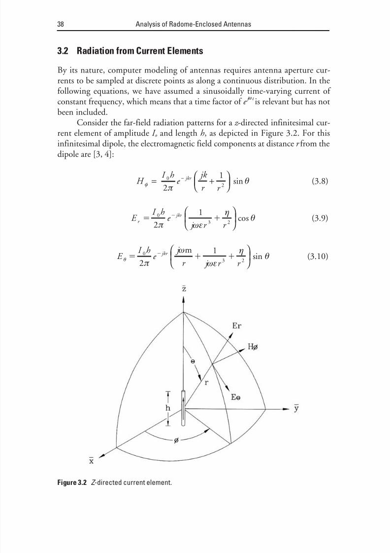
Consider the far-field radiation patterns for a z -directed infinitesimal cur-rent element of amplitude I o and length h , as depicted in Figure 3.2. For thisinfinitesimal dipole, the electromagnetic field components at distance r from thedipole are [3, 4]:
H I h e jk r r
jkr φ
πθ= +
−0
221 sin (3.8)
E I h
e j r r
r jkr 0
3 22
1
π ωε
ηθ
cos (3.9)
E
I h
e
j
r j r r
jkr
θ π
ω
ωε
ηθ 0
3 22
1m
sin (3.10)
38 Analysis of Radome-Enclosed Antennas
Figure 3.2 Z -directed current element.

8/20/2019 Analysis of Radome-Enclosed Antennas
http://slidepdf.com/reader/full/analysis-of-radome-enclosed-antennas 60/319
where E is in volts per meter, H is in amperes per meter, and η is the waveimpedance in ohms given by:
η µε= (3.11)
For most problems of interest, it is only necessary to know the field com-ponents if r is very much greater than a wavelength. For this condition, we may ignore the r 2 and r 3 terms in the above expressions. Under the condition where
we can do this, the only remaining significant electromagnetic field componentsare:
H I h jk
r φ
πθ≈
0
2sin (3.12)
E I h j
r θ
π
ωµθ≈
0
2sin (3.13)
From (3.12) and (3.13), the free-space wave impedance (in air or vacuum)
in the far field is derived as the ratio
η µ
ε πθ
φ
00
0
120 E
H = (3.14)
At a fixed distance, the variation of the electromagnetic field componentsonly contains a sinusoidal variation with a maximum value in the directionorthogonal to the dipole. When modeling an antenna aperture as an ensembleof dipole radiators, we have to account for this variation of the dipole elementpattern.
3.3 Antenna Array Factor
An antenna element radiates an electric field with two polarization components:
( ) ( )E E E θ φθ φ θ θ φ φ, ,+ (3.15)
where E θ and E φ are the two complex electric field components that have a com-mon phase center and θ and φ are unit vectors in the θ and φ directions,respectively.
Antenna Fundamentals 39

8/20/2019 Analysis of Radome-Enclosed Antennas
http://slidepdf.com/reader/full/analysis-of-radome-enclosed-antennas 61/319
Assume an array of N antenna elements, where N is an integer equal to orgreater than two. The total pattern is obtained by adding the electric fields radi-ated from each, as in:
( ) ( )[ ]E E E e i i jkr
n
N
i = , + −
=∑ θ φθ φ θ θ φ φ,
1
(3.16)
We make various approximations in this equation. For instance, we ignoremutual coupling changes in the dipole patterns due to nearby antennas, andonly the isolated element patterns are used. If the antennas all have identical ele-ment patterns, then we can separate (3.16) into a product [4]:
( ) ( )[ ]E E E I e i jkr
n
N
i = + −
=∑θ φθ φ θ θ φ φ, ,
1
(3.17)
where E θ and E φ are the normalized patterns of the electric field from a singleelement with unity current and I i are the relative current weights of the i th ele-ment and generally include amplitude and phase terms originating in the feeddistribution. The (θ, φ) notation indicates that both of the electric field compo-
nents have a θ and φ dependence.Equation (3.17) is a powerful notion since it divides the far-field radiationpattern into an element pattern factor and an array factor. (The element patternis the left-side expression, and the array factor is the right-side expression.) Inthe analysis of a radome-enclosed antenna, we will primarily be interested in theimpact of a radome on the antenna array factor. We will compare the array fac-tor with the radome and the array factor without the radome.
3.4 Linear Aperture Distributions
Assume that an antenna is transmitting and that it is a z -directed current ele-ment with a total array length L a and centered at z = 0, as illustrated in Figure3.3. If the distribution of the radiating current is continuous, the electric andmagnetic fields are [5]
E j e
r I z e dz
jkr
o
j z
L
L
o
a
a
ωµ π
θ π
λθ
4
2
2
2
sin ( )cos
−∫ (3.18)
and
40 Analysis of Radome-Enclosed Antennas
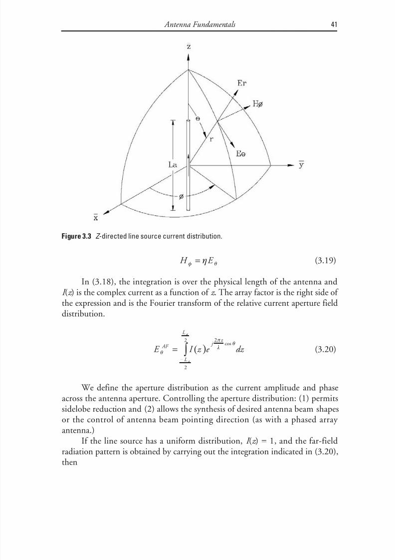
8/20/2019 Analysis of Radome-Enclosed Antennas
http://slidepdf.com/reader/full/analysis-of-radome-enclosed-antennas 62/319
H E φ θ η= (3.19)
In (3.18), the integration is over the physical length of the antenna andI (z ) is the complex current as a function of z . The array factor is the right side of the expression and is the Fourier transform of the relative current aperture fielddistribution.
( )E I z e dz
AF j
z
L
L
a
a
θ
π
λθ
= −∫
2
2
2cos
(3.20)
We define the aperture distribution as the current amplitude and phaseacross the antenna aperture. Controlling the aperture distribution: (1) permitssidelobe reduction and (2) allows the synthesis of desired antenna beam shapesor the control of antenna beam pointing direction (as with a phased array antenna.)
If the line source has a uniform distribution, I (z ) = 1, and the far-fieldradiation pattern is obtained by carrying out the integration indicated in (3.20),then
Antenna Fundamentals 41
Figure 3.3 Z -directed line source current distribution.

8/20/2019 Analysis of Radome-Enclosed Antennas
http://slidepdf.com/reader/full/analysis-of-radome-enclosed-antennas 63/319

8/20/2019 Analysis of Radome-Enclosed Antennas
http://slidepdf.com/reader/full/analysis-of-radome-enclosed-antennas 64/319
Note that the maximum for this current distribution in (3.22) is at thecenter of the current element at z = 0 and that the vertically oriented current ele-ment extends from z = −L a /2 to z = +L a /2. Substituting this into (3.20) and car-
rying out the integration, we obtain
E
L
L AF
a
a θ
π
λθ
π
π
λθ
π
π
=+
+
+1
2
2
2
sin cos
cos
sin L
L
a
a
λθ
π
π
λθ
π
cos
cos
−
−
2
2
(3.23)
We show this pattern also in Figure 3.4 for an antenna that is 0.1m long at
10 GHz. It has −23.5-dB sidelobes, but a greater half-power beamwidth thanthe uniform distribution case. Other antenna aperture distributions that we canapply to this vertical current element for low sidelobe levels include a cosineraised to a power
( )I z z
L n
a
=
cos
π(3.24)
in which n is a power equal to or greater than 0 and need not be an integer. Themaximum for this current distribution in (3.24) is at the center of the currentelement at z = 0, and the vertically oriented current element extends from z =−L a /2 to z = +L a /2. Also, n = 0 reduces to the uniform illumination case.
A parabolic distribution on a pedestal is defined by the following formula:
( ) [ ]( )
I z p p z
L a
= + − −
1 1
0 5
2
2
.
(3.25)
In this equation p is the pedestal parameter and is equal to or less thanunity.
The maximum for this current distribution in (3.25) is also at the center of the current element at z = 0, and the vertically oriented current element extendsfrom z = −L a /2 to z = +L a /2.
For all these distributions, Table 3.1 summarizes the relative gain to the
uniform distribution case, the half-power beamwidth, and the first sidelobelevels. A combination of simpler forms can approximate many other distribu-
tions. For example, to find the directivity pattern of a cosine raised to a power ona pedestal having the form, use the following:
Antenna Fundamentals 43

8/20/2019 Analysis of Radome-Enclosed Antennas
http://slidepdf.com/reader/full/analysis-of-radome-enclosed-antennas 65/319
( ) [ ]I z p p z L
n
a = + −
1 cos π (3.26)
The resulting pattern is the superposition of the pattern obtained for a uniform distribution (this corresponds to the pedestal) and the pattern obtainedfor a cosine raised to the n th power. For instance, for a cosine-squared distribu-tion on a pedestal, the directivity pattern is
( )
E pL
L
L
p L
AF a
a
a
a
θ
π θ λ
π θ
λ
=
+ −
sin cos
cos
1 12
L
L L
a
a a
sin cos
cos cos
π θ
λ
π θ
λ
π
π π θ
λ
−
2
2
2
(3.27)
In a computerized analysis of radome-enclosed antennas, the antenna aperture is generally sampled in discrete increments in accordance with theNyquist criteria. These criteria are analogous to the criteria for keeping grating
44 Analysis of Radome-Enclosed Antennas
Table 3.1
Line Source Pattern Characteristics
DistributionRelativeGain (dB)
Half-Power
BeamwidthHPBW (°)
First NullPosition (°)
First
SidelobeLevel (dB)
Uniform 0 51/(L / ) 57.3/(L / ) 13.2
cos n , where:
n = 1 −0.92 68.75/(L / λ) 85.94/(L / λ) −23
n = 2 −1.76 83.08/(L / λ) 114.59/(L / λ) −32
n = 3 −2.4 95.11/(L / λ) 143.23/(L / λ) −40
n = 4 −2.88 110.58/(L / λ) 171.89/(L / λ) −48
Parabolic, where:
p = 0.8 −0.03 52.71/(L / λ) 60.73/(L / λ) −15.8
p = 0.5 −0.13 55.58/(L / λ) 65.32/(L / λ) −17.1
p = 0.0 −0.79 65.89/(L / λ) 81.93/(L / λ) −20.6

8/20/2019 Analysis of Radome-Enclosed Antennas
http://slidepdf.com/reader/full/analysis-of-radome-enclosed-antennas 66/319
lobes out of real space, as in the case of a phased array antenna. These grating lobes would corrupt antenna pattern data and result in computational errors.
The criterion for determining the maximum sample spacing so that the
nearest grating lobe is on the edge of real space corresponds to the condition [6]:
d
o λ θ≤
+1
1 sin(3.28)
where d / λo is the sample to sample spacing in wavelengths at the operating fre-quency and θo is the direction of maximum radiation. (Most of the antennas tobe addressed in this book have a maximum radiation lobe normal to the antenna
aperture surface.) A sample spacing of a half wavelength is guaranteed to keepgrating lobes out of real space, which will contribute to computational errors. Assume that there are N samples with d z being the interval between sam-
ples, such that L a = Nd z . On this basis, the array factor corresponding to (3.20) will reduce to:
E I e AF n
jkz
n
N n
θθ=
=∑ cos
1
(3.29)
where I n represents the sampled aperture distribution weighting at the n th pointand is generally a complex quantity and z n is the z -coordinate location of the n thpoint where z n = nd z .
3.5 Two-Dimensional Distributions
A method similar to that used for the line source can find the far-field radiation
directivity pattern for a two-dimensional aperture. However, the Fourier trans-form is taken over two dimensions instead of one dimension. For instance,assume that the aperture distribution is in the y -z plane. The array factor is now given by
( ) ( )E I y,z e dydz AF jk x y θ
θ φ φ= +∫∫ sin cos sin (3.30)
This integral can treat circular apertures by defining the appropriate illu-
mination function, I ( y , z ). Note that I ( y , z ) must be zero outside of the circularantenna aperture. To illustrate the use of this integral, consider a circular aper-ture of diameter D a centered at the origin with a parabolic distribution raised toa power n having the form:
Antenna Fundamentals 45

8/20/2019 Analysis of Radome-Enclosed Antennas
http://slidepdf.com/reader/full/analysis-of-radome-enclosed-antennas 67/319
( )( )
I y z y z
D a
n
, = − +
12
2 2
2 (3.31)
Table 3.2 shows the far-field pattern characteristics. Note that the condi-tion for n = 0 corresponds to a uniformly illuminated circular aperture and has−17.6-dB first sidelobe levels. The condition for n = 1 corresponds to a circularaperture parabolic distribution and has reduced sidelobes to −24.6 dB.
A planar aperture two-dimensional transform separates into one-dimen-sional transforms when the aperture distribution involves a product where eachfactor depends on only one coordinate [2], that is, it is product separable of theform
( ) ( ) ( )I y z I y I z , = (3.32)
In this equation, we define the net radiation pattern as the product of theprincipal plane patterns obtained from line source distributions I ( y ) and I (z ),respectively. However, if the aperture distribution is not separable, we mustevaluate a two-dimensional integral numerically.
From Maxwell’s equations, Appendix A develops a formulation for thefar-field radiation patterns of an ensemble of infinitesimal current elements,equally spaced d y apart in the y -plane and d z apart in the z -plane, thus forming a rectangular grid, as illustrated in Figure 3.5. The numerical summation hasgiven the resulting array factor [5]:
( )E I e AF mn
jk md nd
n
N
m
M x y
θ
θ φ φ= +
==∑∑ sin cos sin
11
(3.33)
The m index pertains to the y -coordinate, and the n index pertains to thez -coordinate.
46 Analysis of Radome-Enclosed Antennas
Table 3.2
Circular Aperture Pattern Characteristics
n
Relative
Gain (dB)
Half-Power
Beamwidth
HPBW (°)
First Null
Position (°)
First
Sidelobe
Level (dB)
0 0 58.44/(D / λ) sin-1[1.22/(D / λ)] −17.6
1 −1.25 72.77/(D / λ) sin-1[1.63/(D / λ)] −24.6
2 −2.52 84.22/(D / λ) sin-1[2.03/(D / λ)] −30.6
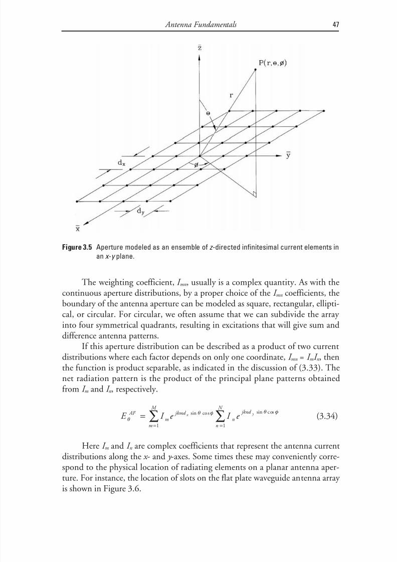
8/20/2019 Analysis of Radome-Enclosed Antennas
http://slidepdf.com/reader/full/analysis-of-radome-enclosed-antennas 68/319
The weighting coefficient, I mn , usually is a complex quantity. As with thecontinuous aperture distributions, by a proper choice of the I mn coefficients, theboundary of the antenna aperture can be modeled as square, rectangular, ellipti-cal, or circular. For circular, we often assume that we can subdivide the array into four symmetrical quadrants, resulting in excitations that will give sum anddifference antenna patterns.
If this aperture distribution can be described as a product of two current
distributions where each factor depends on only one coordinate, I mn = I m I n , thenthe function is product separable, as indicated in the discussion of (3.33). Thenet radiation pattern is the product of the principal plane patterns obtainedfrom I m and I n , respectively.
E I e I e AF m
jkmd n
n
N
m
M jknd
x y
θθ φ θ=
==∑∑ sin cos sin co
11
s φ(3.34)
Here I m and I n are complex coefficients that represent the antenna currentdistributions along the x - and y -axes. Some times these may conveniently corre-spond to the physical location of radiating elements on a planar antenna aper-ture. For instance, the location of slots on the flat plate waveguide antenna array is shown in Figure 3.6.
Antenna Fundamentals 47
Figure 3.5 Aperture modeled as an ensemble of z -directed infinitesimal current elements in
an x -y plane.

8/20/2019 Analysis of Radome-Enclosed Antennas
http://slidepdf.com/reader/full/analysis-of-radome-enclosed-antennas 69/319
3.6 Spiral Antennas
Spiral antennas have frequency-independent radiation patterns and are used in
radome-enclosed direction finding (DF) systems on aircraft, antiradiation hom-ing (ARH) missile guidance systems, and broadband surveillance systems. Anoverview of the historical development of these antennas appears in [7–11].
We generally fabricate planar spiral antennas on a printed circuit (PC)board. To obtain a unidirectional pattern, a lossless cavity is placed on one sideof the spiral. This cavity limits the frequency-independent pattern bandwidth to
48 Analysis of Radome-Enclosed Antennas
Figure 3.6 Waveguide flat plate antenna. (Photo courtesy of Hughes Missile Systems
Division.)

8/20/2019 Analysis of Radome-Enclosed Antennas
http://slidepdf.com/reader/full/analysis-of-radome-enclosed-antennas 70/319
about an octave. Hamel and Scherer [12] have found that an absorber-lined cav-ity can extend a spiral operation to a decade bandwidth.
A two-arm (or log-spiral) antenna, shown in Figure 3.7, is frequency inde-
pendent because angles entirely describe the antennas shape, which make itinvariant to a change of scale [11, 13, 14]. The radius function can be foundfrom the formula
ρ ρ αψ= 0e (3.35)
where a is the expansion coefficient. We rotate the curve of the equation 180°around the origin to define the second arm of the spiral.
We may analyze the planar spiral structure as a strip radiator with currentsflowing along the arms. The inner part of the spirals serves as a nonradiating transmission line, carrying the current out to the active region, which is a nar-row circumferential ring where antenna radiation takes place. The active regions
where radiation takes place correspond to circumferences of m λ in diameter, where m is an integer equal to or greater than unity and is referred to as the mode of the radiation.
Hand rules determine the sense of the circular polarization. For instance,pointing your thumb away from the spiral, let the fingers roll in the direction of
the increasing spiral radius. The hand that must be used determines the polar-ization sense. For instance, if you must use your right hand in order for your fin-gers to roll in the direction of increasing spiral radius, then the spiral antenna isof the right-hand circular polarization (RHCP) sense.
Antenna Fundamentals 49
Figure 3.7 Equiangular spiral antenna geometry.

8/20/2019 Analysis of Radome-Enclosed Antennas
http://slidepdf.com/reader/full/analysis-of-radome-enclosed-antennas 71/319
The Archimedean spiral antenna has constant spacing between adjacentarms, as illustrated in Figure 3.8. It is only frequency independent over a typicaldecade-bandwidth frequency range [15]. However, in order to obtain this com-
plete bandwidth, it requires lossy material on the ends of the arms to eliminateend reflections [16].The Archimedean spiral has a radius function that increases uniformly
with the angle Φ according to
ρ ρ αψ= +o (3.36)
For sufficiently large spiral antennas that support higher-order modes, thecurrents in these modes vary as e jm ψ with ψ varying from 0 to 2 π. All modes for
which m > 1 have a null on boresight. For bandwidths less than 3:1 for a two-arm spiral, the 3 λ diameter ring cannot exist, so that only the principal m =1 mode exists. For greater electrical bandwidths, the control of radiation in thehigher-order modes can be controlled by spiral design methods; an excellent dis-cussion appears in Corzine and Mosko [17].
With four-arm spirals, it is possible to simultaneously excite and isolateboth the mode 1 and mode 2 responses, which appear much like a monopulseantenna sum and difference pattern. We model the spiral by replacing the aper-
ture with two concentric current rings and their proper phase distributions. Themode 1 and mode 2 radiation patterns are shown in Figure 3.9. A phasing tech-nique to obtain these modes is shown in Schuchardt and Kozakoff [18], as illus-trated in Figure 3.10. Each of these modes is rotationally symmetric about the
50 Analysis of Radome-Enclosed Antennas
Figure 3.8 Archimedean spiral antenna geometry.

8/20/2019 Analysis of Radome-Enclosed Antennas
http://slidepdf.com/reader/full/analysis-of-radome-enclosed-antennas 72/319
z-axis, and the field is pure circular polarization, with the polarization sensedetermined by the spiral winding.
Antenna Fundamentals 51
Figure 3.10 Monopulse circuit for four-arm spiral.
Figure 3.9 Radiation patterns for four-arm multimode spiral.

8/20/2019 Analysis of Radome-Enclosed Antennas
http://slidepdf.com/reader/full/analysis-of-radome-enclosed-antennas 73/319
For all planar spiral antennas operating in the principal (m = 1) mode, theantenna must have an outer circumference of 1.25 wavelengths at the lowestoperating frequency. This circumference insures good antenna patterns and
impedance match when the antenna is operating at lowest frequency.
References
[1] Silver, S., Microwave Antenna Theory and Design , New York: McGraw-Hill, 1949.
[2] Jasik, H., “Fundamentals of Antennas,” Ch. 1 in Antenna Engineering Handbook , 3rd ed.,R. C. Johnson, (ed.), New York: McGraw-Hill, 1993.
[3] Eibert, T. F., and J. L. Volakis, “Fundamentals of Antennas, Arrays, and MobileCommunications,” Ch. 1 in Antenna Engineering Handbook , 4th ed., J. Volakis, (ed.),New York: McGraw-Hill, 2007.
[4] Milligan, T. A., Modern Antenna Design, 1st ed., New York: McGraw-Hill, 1986.
[5] Johnson, R. C., “Fundamentals of Antennas,” and “Arrays of Discrete Elements,” Chs. 2and 3 in Antenna Engineering , 3rd ed., R. C. Johnson, (ed.), New York: McGraw-Hill,1993.
[6] Mailloux, R. J., Phased Array Antenna Handbook , Norwood, MA: Artech House, 1994.
[7] Jordan, E. C., et al., “Developments in Broadband Antennas,” IEEE Spectrum , Vol. 1, April 1964, pp. 58–71.
[8] Wang, J. J. H., and V. K. Tripp, “Design of Multi-Octave Spiral-Mode Microstrip Anten-nas,” IEEE Transactions on Antennas and Propagation , Vol. 39, No. 3, March 1991, pp.332–335.
[9] Cubley, H. D., and H. S. Hayre, “Radiation Field of Spiral Antennas Employing Multimode Slow Wave Techniques,” IEEE Transactions on Antennas and Propagation , Vol.
AP-19, January 1971, pp. 126–128.
[10] Dyson, J. D., “The Characteristics and Design of the Conical Spiral Antennas,” IEEE Transactions on Antennas and Propagation, Vol. AP-13, July 1965, pp. 488–499.
[11] Deschamps, G. A., and J. D. Dyson, “The Logarithmic Spiral in a Single-ApertureMulti-Mode Antenna System,” IEEE Transactions on Antennas and Propagation , Vol.
AP-19, January 1971, pp. 90–95.
[12] Du Hamel, R. H., and J. P. Scherer, “Frequency Independent Antennas,” Ch.14 in Antenna Engineering Handbook , 2nd ed., R. C. Johnson and H. Jasik (eds), New York:McGraw-Hill, 1984.
[13] Rumsey, V. H., “Frequency Independent Antennas,” IRE National Convention Record ,Part 1, 1957, pp. 114–118.
[14] Dyson, J. D., “The Equiangular Spiral,” IRE Transactions on Antennas and Propagation ,Vol. AP-7, No. 2, April 1959, pp. 181–187.
[15] Turner, E. M., “Spiral Slot Antenna,” U.S. Patent 2,863,145, December 1958.
52 Analysis of Radome-Enclosed Antennas

8/20/2019 Analysis of Radome-Enclosed Antennas
http://slidepdf.com/reader/full/analysis-of-radome-enclosed-antennas 74/319
[16] Rudge, A. W., et al., The Handbook of Antenna Design , 2nd ed., London, England: PeterPeregrinus Ltd, on behalf of the Institution of Electrical Engineers (UK), 1986.
[17] Corzine, R. G., and J. A. Mosko, Four Arm Spiral Antennas , Norwood, MA: ArtechHouse, 1990.
[18] Schuchardt, J. M., and D. J. Kozakoff, “Seeker Antennas,” Ch. 46, Antenna Engineering Handbook , 4th ed., J. Volakis, (ed.), New York: McGraw-Hill, 2007.
Antenna Fundamentals 53

8/20/2019 Analysis of Radome-Enclosed Antennas
http://slidepdf.com/reader/full/analysis-of-radome-enclosed-antennas 75/319

8/20/2019 Analysis of Radome-Enclosed Antennas
http://slidepdf.com/reader/full/analysis-of-radome-enclosed-antennas 76/319
4Radome Dielectric Materials
In analyzing radome electrical performance, it is important to evaluate the elec-trical properties of possible radome wall materials at various wavelengths. Theprimary electrical properties of candidate materials are the relative dielectric con-stant and the loss tangent of the candidate materials at the operationalfrequencies of the radome.
The structural (aeromechanical) and environmental requirements deter-
mine other parameters for a candidate radome material and include:
• Mechanical properties, such as flexural moduli, strength, and hardness;
• Material density;
• Water absorption;
• Rain erosion (particle impact) resistance;
• The variation of both the mechanical and electrical parameters of the
material due to temperature variations.
This chapter focuses on the electrical properties of selected radome wallmaterials as they influence the electrical design of a radome. Mechanical andphysical data for candidate materials are readily available in many sources, suchas the biannual Proceedings of the Symposium on Electromagnetic Windows[1–9]. A survey of the properties of many avionics radome materials was pub-lished in a NATO funded report [10], a survey of ceramics materials appear in
[11], a review of moldable organic (plastic) materials is found in a USAF publi-cation [12], and an electromagnetic window material data handbook was pre-pared by the IIT Research Institute and Purdue University [13] that addresses
55

8/20/2019 Analysis of Radome-Enclosed Antennas
http://slidepdf.com/reader/full/analysis-of-radome-enclosed-antennas 77/319
the multispectral performance of candidate materials. Lastly, since the first edi-tion of this book, Burks has published some updated radome material data in[14].
4.1 Organic Materials
Most civilian/military aircraft, ground vehicles, and fixed terrestrial radomes useorganic radome wall materials. Organic radome materials are useful at maxi-mum service temperatures below 1,000°F (the maximum temperature depend-ent on the material chosen); at temperatures above the service temperature, both
the mechanical and electrical parameters rapidly degrade to unacceptable values.Radome wall construction is typically one of the following categories:
• Solid (monolithic ), generally made of resins incorporating reinforce-ments such as chopped glass fibers;
• Sandwich design, consisting of alternating high-density (high relativedielectric constant) and low-density (low relative dielectric constant)materials.
4.1.1 Monolithic Radomes
Many radomes, particularly of the electrically thin wall variety, use a single-layer wall material and are termed monolithic wall radomes. Monolithic radomesoften incorporate some type of fiber reinforcement in order to enhance themechanical properties of the resin material. For this case, we obtain the resulting
relative dielectric constant of the mixture from
ε ε ε
m R R F F
R F
V V
V V =
++
log log (4.1)
where
εm = relative dielectric constant of mixture;
εR
= relative dielectric constant of the resin;
εF = relative dielectric constant of reinforcement fibers;
V R = volume of the dielectric resin;
V F = volume of reinforcement fibers.
Equation (4.1) assumes that the mixture is uniform and isotropic.
56 Analysis of Radome-Enclosed Antennas

8/20/2019 Analysis of Radome-Enclosed Antennas
http://slidepdf.com/reader/full/analysis-of-radome-enclosed-antennas 78/319
Occasionally, particularly at millimeter-wave bands, monolithic radomesare used without reinforcement. Table 4.1 shows the dielectric properties of sev-eral of these materials [15, 16].
The fabrication method for small monolithic wall radomes includes com-pound or injection molding, and even possibly machining. Fabrication of largermonolithic wall radomes might use a wet layup on a mandrel of the desiredradome shape.
4.1.2 Sandwich Radomes
Throughout the microwave spectrum, sandwich radomes that include low-den-sity core materials and higher-density skin materials are popular because sand-
wich radomes are more broadband than monolithic radomes and also have a higher strength-to-weight ratio.
4.1.2.1 Prepreg Materials
The more dense layers typically are fabricated from a fiber-reinforced resin sys-tem. Table 4.2 shows the approximate dielectric properties of some popularfiber reinforcement and resin systems [10, 11; personal communication withBen MacKenzie, Saint Gobain Performance Plastics (formerly Norton Perfor-
mance Plastics), Ravenna, Ohio, 1996].The radome designer must consider both the electrical and mechanicalproperties in selecting a reinforcement. Some of these properties are listed here:
• S-glass, a silica-alumina-magnesia composite, is a high-strength glass where the reinforcement fibers’ tensile strength is maintained to 650°C.
• E-glass contains alumina-borosilicate and is low-cost. Compared withS-glass, it shows a greater reduction of tensile strength at 650°C.
Radome Dielectric Materials 57
Table 4.1
Approximate Dielectric Properties of Some Common Plastics
Material
Relative
Permittivity,
X-Band
Loss
Tangent,
X-Band
Relative
Permittivity,
Ka-Band
Loss
Tangent,
Ka-Band
Rexolite 2.54 0.0005 2.6 0.002
Nylon 3.03–3.21 0.014–0.02 3.6 0.02Teflon 2.1 0.0003 2.08–2.10 0.0006–0.001
Polystyrene 2.55 0.0004 2.54 0.00053–0.001
lparPlexiglass 2.59 0.015 2.61 0.02
Polyethylene 2.25 0.0004 2.28 0.007

8/20/2019 Analysis of Radome-Enclosed Antennas
http://slidepdf.com/reader/full/analysis-of-radome-enclosed-antennas 79/319

8/20/2019 Analysis of Radome-Enclosed Antennas
http://slidepdf.com/reader/full/analysis-of-radome-enclosed-antennas 80/319
Performance Plastics (formerly Norton Performance Plastics), Ravenna, Ohio,1996].
The sheet prepreg laminate comes with precise and uniform resin contentthrough the wall. Thus, tolerances can be controlled to a desired thickness moreaccurately than with the wet-layup approach. Prepreg material is commercially available in commonly used discrete thicknesses that are multiples of one ply (i.e., about 11 mils per ply). Special-order plies are available in a nonstandardthickness of a half ply (i.e., 5.5 mils for a half ply).
Note that in radome electrical design, it will be shown that the least thick-ness dense layers (least number of plies) results in the best bandwidth and theleast radome losses. Marine, terrestrial, or vehicular sandwich radomes could useas few as one ply for the dense layers. However, for aircraft applications thenumber of plies required is dictated by the aeromechanical environment. Very slow-moving aircraft or unmanned air vehicles (UAVs) might use as few as oneor two plies. Commercial jet aircraft may use three or four plies for the denselayers of aircraft sandwich radomes.
4.1.2.2 Core Materials
Honeycomb and foam are both extremely lightweight and strong materials thatare commonly used for the low-density layer of sandwich radomes.
Radome Dielectric Materials 59
Table 4.3
Approximate Dielectric Properties of Selected Laminates (X-Band Data)
Reinforcement Resin
Relative
Permittivity Loss Tangent
E-glass Epoxy
Polyester
Polyimide
4.4
4.15
4.7
0.016
0.015
0.014
D-glass Polycyanate 3.45 0.009
Polyethylene (Spectra) Epoxy
Polyester
Polycyanate
2.8
2.52
2.65
0.004
0.007
0.003
Kevlar Polyester 3.5 0.05Quartz Epoxy
Polyester
Polyimide
Polycyanate
Polybutadiene
Bismaleimide
3.12
3.6
3.34
3.23
3.1
3.35
0.011
0.012
0.005
0.006
0.003
0.009

8/20/2019 Analysis of Radome-Enclosed Antennas
http://slidepdf.com/reader/full/analysis-of-radome-enclosed-antennas 81/319
Reinforced plastic honeycomb materials as illustrated in Figure 4.1 areavailable in a variety of wall resins and reinforcements that operate over a widetemperature range. Nomex honeycomb has been the leading structural honey-
comb core in the aerospace industry. Nomex operates to 350°F, is an aramidhoneycomb core material, and has a relative dielectric constant on the order of 1.1 and a loss tangent less than 0.005 [36]. Korex honeycomb is available insmall cell sizes and low densities like the honeycomb of Nomex aramid. Wereinforce it with high modulus aramid fibers and a phenolic resin. However,stiffness in shears and compression of the core are about double those of thearamid cores. Korex electrical properties are the same as Nomex.
Standard glass-reinforced honeycombs with phenolic resins operate to350°F. These honeycombs have a relative dielectric constant on the order of
1.35 and a loss tangent of 0.001. Anisotropy of honeycomb cores can become a problem at millimeter-wave frequencies. Many other honeycomb materials areavailable for higher-temperature operation, such as glass reinforcement with a polyimide resin system, which operates to 500°F.
Dielectric foam materials have also been used for the low-density layers of sandwich radomes as a substitute for honeycomb materials previously discussed.
At microwave frequencies either may be used with essentially no difference inperformance. However, at millimeter-wave frequencies many radome designers
have found that waveguide type behavior of the honeycomb cells results in dete-riorated performance of a sandwich radome from the theoretically predicted
60 Analysis of Radome-Enclosed Antennas
Figure 4.1 Phenolic honeycomb core material photo.
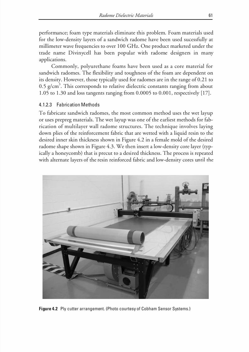
8/20/2019 Analysis of Radome-Enclosed Antennas
http://slidepdf.com/reader/full/analysis-of-radome-enclosed-antennas 82/319

8/20/2019 Analysis of Radome-Enclosed Antennas
http://slidepdf.com/reader/full/analysis-of-radome-enclosed-antennas 83/319
desired number of layers and total thickness is obtained. Note that using a female mold in the final resin-reinforced fabric plies represents the innermostradome layer.
When the layup is completed, a plastic (vacuum) bag is placed over thecomplete layup, thereby sealing the mold. The plastic bag is connected to a vac-uum pump that evacuates the air between the bag and the layup. The completemold is then inserted in an autoclave to cure the sandwich under heat and pres-
sure; a typical autoclave used for this purpose is shown in Figure 4.4. By thisfabrication process, the tolerance on skins is typically plus or minus 1 mil oneach ply of the dense layers.
The state-of-the-art method of sandwich radome fabrication uses prepreg materials that are resin-preimpregnated fabric-reinforced laminates. The meth-odology is near identical to the wet layup; however, resins do not have to beapplied since the material is preimpregnated with resins. The fabrication toler-ance using prepreg materials is very good compared to the wet layup method.
4.2 Inorganic Materials
The mechanical strength of most organic wall materials deteriorates at 250°C,and even the best can only survive for a short time at 500°C [18]. Therefore,
62 Analysis of Radome-Enclosed Antennas
Figure 4.3 Female radome mold fixture. (Photo courtesy of Cobham Sensor Systems.)

8/20/2019 Analysis of Radome-Enclosed Antennas
http://slidepdf.com/reader/full/analysis-of-radome-enclosed-antennas 84/319
high-temperature applications, such as hypersonic missiles, often usenonorganic (ceramic) type radome materials. Table 4.4 lists representative val-ues for nonorganic radome materials.
Most of these materials have suitable electrical properties for high-velocity radome applications, such as missiles. For instance, alumina (aluminum oxide)and Pyroceram and Rayceram (both cordierite) have been widely used for flightvehicles operating at and below about Mach 4. They are hard and have fair rain
erosion resistance, but are difficult to grind to shape. Pyroceram has a higherdielectric constant than either Rayceram or alumina, which implies tightermechanical tolerances in manufacture.
Many ceramic materials have a high thermal expansion and are susceptibleto thermal shock resulting from rapidly forming temperature gradients during flight. Shock causes the dome to fracture, particularly if the radome is under a mechanical loading. For instance, a 400°C differential may result in failure dueto the thermal shock for an alumina radome [11]. Therefore, the radome
designer must take care in material selection.Slip cast fused silica (SCFS), a form of silicon oxide, is suited for high-tem-
perature applications. It has good electrical properties, low cost, and a thermalexpansion coefficient less than either alumina or cordierite materials, which
Radome Dielectric Materials 63
Figure 4.4 Autoclaves. (Photo courtesy of Cobham Sensor Systems.)

8/20/2019 Analysis of Radome-Enclosed Antennas
http://slidepdf.com/reader/full/analysis-of-radome-enclosed-antennas 85/319
improves its thermal shock capability. It has been used on reentry vehicles atover Mach 8 velocities.
A high-temperature resin was developed for use in quartz-based 3D com-posites and in chopped fiber-filled molding compounds [19]. This 3D quartzhas good thermal shock resistance and finds application for hypersonic missilesor reentry antenna windows. Structures fabricated from this material have beentested at over 1,900°C with a negligible change in transmission.
A radome designer must be concerned by the variation of a dielectric con-
stant and loss tangent with increasing temperatures since the loss tangent of thematerial must be kept low to achieve high radome transmissivity. Figure 4.5shows representative data for SCFS, Pyroceram, and Rayceram. As with thedielectric constant, the loss tangent also increases with increasing temperature.The variation of these properties with temperature can result in disastrousresults in the antenna performance if not accounted for in a particular radomeapplication, for instance, thermally increased transmission loss to an unaccept-able level or thermally increased BSE or BSES, which might result in an unstableguidance system. Figure 4.6 is a photo of thin wall ceramic radomes.
Researchers at the Georgia Institute of Technology have evaluated siliconnitride [20] and found it to have good electrical properties, mechanical strength,and high rain erosion and thermal shock resistance. They have investigated it intwo forms:
64 Analysis of Radome-Enclosed Antennas
Table 4.4
Dielectric Properties of Selected Ceramic Materials (X-Band Data)
Materials
Relative
Permittivity Loss Tangent
Alumina 9.4–9.6 0.0001–0.0002
Boron nitride 4.2–4.6 0.0001–0.0003
Beryllia 4.2 0.0005
Borosilicate glass 4.5 0.0008
Pyroceram 5.54–5.65 0.0002
Rayceram 4.70–4.85 0.0002
Slip cast fused silica (SCFS) 3.30–3.42 0.0004Woven (3D) quartz 3.05–3.1 0.001–0.005
Silicon nitride (HPSN) 7.8–8.0 0.002–0.004
Silicon nitride (RSSN) 5.6 0.0005–0.001
Nitro-oxyceram 5.2 0.002
Reinforced Celsian 6.74 0.0009

8/20/2019 Analysis of Radome-Enclosed Antennas
http://slidepdf.com/reader/full/analysis-of-radome-enclosed-antennas 86/319
Radome Dielectric Materials 65
Figure 4.5 Slip cast fused silica (SCFS), Rayceram, and Pyroceram variations of electrical
properties with temperature: (a) relative permittivity and (b) loss tangent.

8/20/2019 Analysis of Radome-Enclosed Antennas
http://slidepdf.com/reader/full/analysis-of-radome-enclosed-antennas 87/319
• Reaction sintered silicon nitride (RSSN) is formed by reaction of silicon
with nitrogen in which a flame spray molds silicon powder to shape.• Hot pressed silicon nitride (HPSN) forms from the reaction of silicon
with nitrogen to form a powder that can be hot pressed. HPSN is a more dense material than RSSN.
Although silicon nitride generated great interest during the 1980s, to date,only very small radomes have been produced, with some fabrication problemsstill unresolved.
Several advanced ceramic composites have been researched for applications where high-temperature microwave transparency must be combined with goodstrength and all-weather capability [21]. These composites are:
• Nitro-oxyceram, a family of composite materials fabricated from a mix-ture of silicon nitride, boron nitride, and silica. These materials are fab-ricated by hot pressing or hot isostatic processing.
• Celsian, a high-purity barium aluminosilicate. This material exhibitsmechanical strength that is typically six times greater than silica with a much higher rain erosion resistance.
66 Analysis of Radome-Enclosed Antennas
Figure 4.6 Thin wall ceramic radomes. (Photo courtesy of Lockheed Martin Electronics and
Missile Systems.)

8/20/2019 Analysis of Radome-Enclosed Antennas
http://slidepdf.com/reader/full/analysis-of-radome-enclosed-antennas 88/319
Measured permittivity data for a number of other ceramic materials waspublished in [22, 23].
4.3 Dual Mode (RF/IR) Materials
Many modern military sensors use dual-mode operation for improved targetrecognition capability. While most of these sensors currently use individual sen-sor windows for the infrared (IR) and for the RF (microwave or millimeter
waves) ranges, increasingly users are interested in consolidating both sensors, which permits a single electromagnetic window for both.
Typical IR sensors generally operate in either the near-IR (0.45- to
1.2-micron wavelengths), the mid-IR (3- to 5-micron wavelengths), or thefar-IR (8- to 12-microns wavelength) ranges. These wavelengths generally corre-spond to atmospheric windows where propagation losses are acceptable.
4.3.1 Nonorganic Dual-Mode Materials
Table 4.5 shows the IR transmittance ranges versus the wavelength for many optical materials. Variations in transmittance of a given material occur becauseof: (1) manufacturing process differences among suppliers, (2) material impuri-ties, and (3) crystalline structure differences.
The candidates in the list of optical materials become fewer when both of the following requirements for the radome are considered:
• A small loss tangent, that is, preferably tan α < 0.01 in the microwave/millimeter-wave band of interest;
• If for an airborne application, the thermal and mechanical requirementsfor the flight regime.
Selection factors are dependent on the application and include mechanicalstrength, hardness, coefficients of expansion, thermal shock resistance, tempera-ture range of operation, and stability of permittivity (or refractive index) withtemperature. Another concern of currently available optics materials is poorthermal shock resistance.
Researchers at the Georgia Institute of Technology conducted studies of
the potential of zinc selenide (ZnSe) and zinc sulfide (ZnS) for optical windows[24]. Texas Instruments (TI) has investigated gallium arsenide (GaAs) as a potential dual-mode material [25]. GaAs is much harder and more resistant torain erosion than either ZnS or ZnSe. General Electric (GE) has researchedchemically deposited silicon nitride as a dual-mode window [26]. GTE Labora-tories has also done studies of transparent polycrystalline yttria for IR
Radome Dielectric Materials 67

8/20/2019 Analysis of Radome-Enclosed Antennas
http://slidepdf.com/reader/full/analysis-of-radome-enclosed-antennas 89/319
applications [27]. Domes could be isostatically pressed and sintered, which is aneconomical fabrication process. Also, GTE Laboratories report near net shapesintering, which should reduce the cost of grinding and polishing.
The Office of Naval Research (ONR) conducted a study that identified
about 30 ceramic materials suitable for dual-mode windows [28]. Theseinclude:
• Mullite;
• Germanium mullite;
68 Analysis of Radome-Enclosed Antennas
Table 4.5
Transmission Ranges Versus Wavelength for Selected Optical Materials
Material Transmission Wavelengths
Minimum
(Microns)
Maximum
(Microns)
Lithium fluoride(LiF) 0.11 6.0
Magnesium fluoride (MgF2) 0.12 7.0
Calcium fluoride (CaF2) 0.13 8.0
Barium fluoride (MgF2) 0.14 12.0
Quartz (SiO2) 0.15 3.0
UV fused silica (SiO2) 0.16 2.5IR fused silica (SiO2) 0.22 3.3
Glass (BK-7) 0.40 1.4
Silicon (Si) 0.45 7.0
Germanium (Ge) 0.18 12.0
Zinc sulfide (ZnS) 0.40 13.0
Gallium arsenide (GaAs) 1.00 14.0
Sodium chloride (NaCl) 0.18 16.0
Zinc selenide (ZnSe) 0.60 28.0
Potassium chloride (KCl) 0.19 20.0
Potassium bromide (KBr) 0.21 25.0
Cadmium telluride (CdTe) 1.00 25.0
Silver chloride (AgCl) 0.40 29.0
Silver bromide (AgBr) 0.45 35.0
Thallium bromoiodide (KRS-5) 0.60 39.0
Cesium bromide (CaBr) 0.22 50.0
Cesium iodide (CeI) 0.25 60.0

8/20/2019 Analysis of Radome-Enclosed Antennas
http://slidepdf.com/reader/full/analysis-of-radome-enclosed-antennas 90/319

8/20/2019 Analysis of Radome-Enclosed Antennas
http://slidepdf.com/reader/full/analysis-of-radome-enclosed-antennas 91/319

8/20/2019 Analysis of Radome-Enclosed Antennas
http://slidepdf.com/reader/full/analysis-of-radome-enclosed-antennas 92/319
4.4.1 Receiver Noise
It is customary to model a receiver system as noiseless, but account for the noiseat the output by a noise factor F where the noise factor is a dimensionless quan-
tity. The noise can be of a thermal origin (thermal noise) or it can be from othernoise-generating processes. Most of these other processes generate noise whosespectrum and probability distributions are similar to that of thermal noise. Toconsider how we model the effects of noise in a receiver, consider a singlereceiver subsystem stage illustrated in Figure 4.7(a). Using the well-known lawsof black body radiation, the total noise at the output of this single-stageelectronic subsystem is [32, 33]:
P k T BGF no b o = (4.2)
where
G = subsystem power gain (dimensionless);
B = noise bandwidth of the system (Hz);
k b = Boltzmann’s constant = 1.38 × 10
−23 w-s/K;
T o = ambient temperature = 290K.
The quantity K b T o B is the actual thermally generated noise power refer-enced to the input port of the subsystem. Given that the noise figure is the noisefactor expressed in decibels:
( )NF F = 10 log (4.3)
we can express the noise factor in terms of the noise figure
Radome Dielectric Materials 71
(b)
(a)
Figure 4.7 Representation of noisy receiver stages: (a) single stage and (b) two stages in
cascade.

8/20/2019 Analysis of Radome-Enclosed Antennas
http://slidepdf.com/reader/full/analysis-of-radome-enclosed-antennas 93/319
F NF = 10 10 (4.4)
Alternatively, we can account for subsystem generated noise via a
noise-free termination at a temperature T e . The total noise at the output of thesingle-stage subsystem is then
P k T BG no b e = (4.5)
from which we see that the equivalent noise temperature is related to the noisefactor via
T T F e o = (4.6)
This equivalent noise temperature would produce the same noise power atthe output.
Note consider two cascaded receiver subsystems illustrated in Figure4.7(b). Assuming that the bandwidth of the two cascaded stages is the same (B 1= B 2 = B ), then the total thermal noise at the output of the second stage can beshown to be:
( )P k T BG G F F G
k T BG G F no b o b o e = + −
=1 2 1
2
1
1 21 (4.7)
with the equivalent noise factor
F F F
G e = +
−1
2
1
1(4.8)
The equivalent noise factor is approximately equal to the noise factor of the first stage if the gain of the first stage is at least 10. This result is particularly relevant in low-noise receiving systems where the first stage is usually a low-noiseamplifier (LNA) and the second stage is representative of the microwavereceiver; here F e ≈F LNA . In SATCOM systems, the noise factor of the LNA there-fore sets the noise factor for the entire receive system. The state of the art in theC-band LNAs is less than 10K.
Finally, the effective noise temperature may be defined in terms of the sys-tem noise factor as in [34, 35]:
( )T T F
F
G e o = +
−
1
2
1
1(4.9)
72 Analysis of Radome-Enclosed Antennas

8/20/2019 Analysis of Radome-Enclosed Antennas
http://slidepdf.com/reader/full/analysis-of-radome-enclosed-antennas 94/319
Note that the above expressions only apply for a particular terminating impedance at the receiver input. If another value were used, the noise tempera-ture expressions change. Many microwave receiver systems use 50-ohm coaxial
transmission lines, and antennas are matched for the 50-ohm receiver loadimpedance.
4.4.2 Noise Temperature Without Radome
For an antenna connected to a receiver, the system noise temperature isapproximately
T T T sys a e = + (4.10)
Here, T a is the antenna noise temperature and is the noise power seen atthe output terminals of the antenna. The term T e represents the noise tempera-ture of the receiver electronics representative of the noise generated by itsnonideal components and is approximately equal to the noise temperature of theLNA as previously discussed.
Consider that the receiver G/T is the figure of merit at the receiverantenna and is:
( )G T G T T a a e = − +10 log (4.11)
4.4.3 Noise Temperature with Radome
Placed over an antenna, a radome having a power loss L dB can seriously degradethe receive system noise temperature. Consider a radome enclosed antenna illus-trated in Figure 4.8. The noise is the total of internally and externally generatednoise. The main contributors to the total system noise temperature are given in
the following equation:
Radome Dielectric Materials 73
Figure 4.8 Satellite receiving antenna enclosed in a radome of loss L r .

8/20/2019 Analysis of Radome-Enclosed Antennas
http://slidepdf.com/reader/full/analysis-of-radome-enclosed-antennas 95/319
( )T T L L T sys a r r e = + − +290 1
where
T sys = system noise temperature in degrees K;T
a = Antenna noise temperature in degrees K;
T e = Electronics noise temperature in degrees K;
and the radome loss factor is related to the radome loss in decibels (L dB ) via
L r Ldb = 10 10
Note that L r = 1 for a lossless radome. The noise temperature introduced
by the radome loss is the temperature you would have to thermally heat theradome if it were lossless in order to get the same noise power contribution. Theantenna noise temperature T a can be computed from the antenna’s radiationpattern and its surrounding environment. A zenith-pointing satellite antenna may have an antenna temperature in the order of 10K due to the low cosmic(galactic) sky temperature.
The G/T ratio is then:
( )( )G T G T L L T a a r r e = − + − +10 290 1log
74 Analysis of Radome-Enclosed Antennas
Figure 4.9 Additive system noise due to a heated lossy radome.
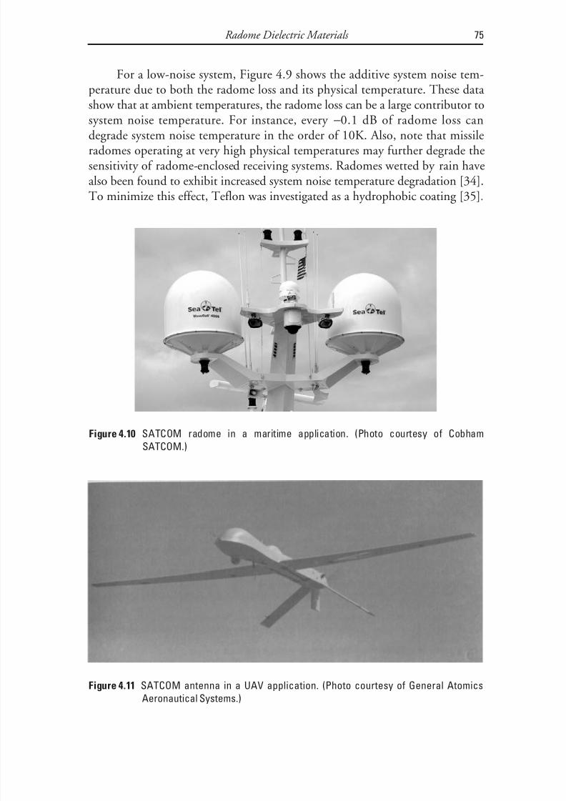
8/20/2019 Analysis of Radome-Enclosed Antennas
http://slidepdf.com/reader/full/analysis-of-radome-enclosed-antennas 96/319
For a low-noise system, Figure 4.9 shows the additive system noise tem-perature due to both the radome loss and its physical temperature. These data show that at ambient temperatures, the radome loss can be a large contributor to
system noise temperature. For instance, every −0.1 dB of radome loss candegrade system noise temperature in the order of 10K. Also, note that missileradomes operating at very high physical temperatures may further degrade thesensitivity of radome-enclosed receiving systems. Radomes wetted by rain havealso been found to exhibit increased system noise temperature degradation [34].To minimize this effect, Teflon was investigated as a hydrophobic coating [35].
Radome Dielectric Materials 75
Figure 4.10 SATCOM radome in a maritime application. (Photo courtesy of Cobham
SATCOM.)
Figure 4.11 SATCOM antenna in a UAV application. (Photo courtesy of General Atomics
Aeronautical Systems.)

8/20/2019 Analysis of Radome-Enclosed Antennas
http://slidepdf.com/reader/full/analysis-of-radome-enclosed-antennas 97/319
The effectiveness of various commercially available hydrophobic coatings islisted in [29].
To illustrate several radome applications in which these considerations
apply, Figure 4.10 shows a shipboard radomes placed over several SATCOMantennas, and Figure 4.11 shows a SATCOM radome installed on a smallaircraft.
References
[1] Bassett, H. L., and J. M. Newton, (eds.), Proceedings of the 13th Symposium on Electromag- netic Windows , Georgia Institute of Technology, Atlanta, GA, September 1976.
[2] Harris, J. N., (ed.), Proceedings of the 14th Symposium on Electromagnetic Windows , Geor-gia Institute of Technology, Atlanta, GA, June 1978.
[3] Bassett, H. L., and G. K. Huddleston, (eds.), Proceedings of the 15th Symposium on Electro- magnetic Windows , Georgia Institute of Technology, Atlanta, GA, June 1980.
[4] Huddleston, G. K., (ed.), Proceedings of the 16th Symposium on Electromagnetic Windows ,Georgia Institute of Technology, Atlanta, GA, June 1982.
[5] Bassett, H. L., (ed.), Proceedings of the 17th Symposium on Electromagnetic Windows , Geor-gia Institute of Technology, Atlanta, GA, July 1984.
[6] Harris, J. N., (ed.), Proceedings of the 18th Symposium on Electromagnetic Windows , Geor-gia Institute of Technology, Atlanta, GA, September 1986.
[7] Handley, J. C., (ed.), Proceedings of the 19th Symposium on Electromagnetic Windows , Geor-gia Institute of Technology, Atlanta, GA, September 1988.
[8] Ohlinger, W. L., (ed.), Proceedings of the 20th Symposium on Electromagnetic Windows ,Georgia Institute of Technology, Atlanta, GA, September 1992.
[9] Handley, J. C., (ed.), Proceedings of the 21st Symposium on Electromagnetic Windows , Geor-
gia Institute of Technology, Atlanta, GA, January 1995.
[10] Cary, R. H., Avionics Radome Materials , North Atlantic Treaty Organization (NATO)Report AGARD-AR-75, London, Technical Editing and Reproduction Ltd., 1974.
[11] Walton, J. D., Radome Engineering Handbook , New York: Marcel Dekker, 1970.
[12] Ossin, A., et al., Millimeter Wavelength Radomes , Report AFML-TR-79-4076, WrightPatterson Air Force Base, OH, AF Materials Laboratory, 1979.
[13] Gibson, C. C., R. H. Bogaard, and D. L. Taylor, “The EM Window Material Database: A Progress Report,” Proceedings of the 21st Symposium on Electromagnetic Windows , Georgia
Institute of Technology, Atlanta, GA, January 1995.
[14] Burkes, D. G., “Radomes,” Ch. 53 in Antenna Engineering Handbook , 4th ed., J. L.Volakis, (ed.), New York: McGraw-Hill, 2007.
[15] Skolnik, M. I., Radar Handbook, New York, McGraw-Hill, 1970.
76 Analysis of Radome-Enclosed Antennas

8/20/2019 Analysis of Radome-Enclosed Antennas
http://slidepdf.com/reader/full/analysis-of-radome-enclosed-antennas 98/319
[16] Newton, J. M., D. J. Kozakoff, and J. M. Schuchardt, “Methods of Dielectric MaterialCharacterization at Millimeter Wavelengths,” Proceedings of the 15th Symposium on Elec- tromagnetic Windows , Georgia Institute of Technology, Atlanta, GA, June 1980.
[17] Rudge, A. W., et al., The Handbook of Antenna Design , IEEE Electromagnetic WavesSeries, London: Peter Peregrinus Ltd., 1986.
[18] Coy, T. N., “Hot Pressed Silicon Nitride,” Proceedings of the 11th Symposium on Electromagnetics Windows , Georgia Institute of Technology, Atlanta, GA, 1972.
[19] Favaloro, M. R., “A Dielectric Composite Material for Advanced Radome and Antenna Window Applications,” Proceedings of the 20th Symposium on Electromagnetic Windows ,Georgia Institute of Technology, Atlanta, GA, September 1992.
[20] Walton, J. D., “Reaction Sintered Silicon Nitride,” Proceedings of the 11th Symposium on Electromagnetics Windows , Georgia Institute of Technology, Atlanta, GA, 1972.
[21] Wright, J. M., J. F. Meyers, and E. E. Ritchie, “Advanced Ceramic Composites for Hyper-sonic Radome Applications,” Proceedings of the 20th Symposium on Electromagnetic Win- dows , Georgia Institute of Technology, Atlanta, GA, September 1992.
[22] Sheppard, A. P., A. McSweeney, and K. H. Breeden, “Submillimeter Wave Material Prop-erties and Techniques,” Proceedings of the Symposium on Submillimeter Waves , PolytechnicInstitute of Brooklyn, NY, 1970.
[23] Nickel, H. U., and R. Heidinger, “A Survey of Vacuum Windows for High Energy Milli-meter Wave Systems in Fusion Experiments,” Proceedings of the 20th Symposium on Elec-
tromagnetic Windows , Georgia Institute of Technology, Atlanta, GA, September 1992.
[24] Papis, J., B. DiBeneditto, and A. Swanson, “Low Cost Zinc Selenide and Zinc Sulfide forFLIR Optics,” Proceedings of the 13th Symposium on Electromagnetic Windows , Georgia Institute of Technology, Atlanta, GA, 1976.
[25] Purinton, D., “GaAs IR-RF Window Material,” Proceedings of the 13th Symposium on Elec- tromagnetic Windows , Georgia Institute of Technology, Atlanta, GA, 1976.
[26] Tanzilli, R. A., J. J. Gebhardt, and J. O. Hanson, “Potential of Chemically Vapor Depos-ited Silicon Nitride as a Multimode EM Window,” Proceedings of the 14th Symposium on
Electromagnetic Windows , Georgia Institute of Technology, Atlanta, GA, 1978.
[27] Rhodes, W. H., “Transparent Polycrytalline Yttria for IR Applications,” Proceedings of the 16th Symposium on Electromagnetic Windows , Georgia Institute of Technology, Atlanta,GA, 1982.
[28] Musikant, S., et al., “Advanced Optical Ceramics,” Proceedings of the 15th Symposium on Electromagnetic Windows , Georgia Institute of Technology, Atlanta, GA, 1976.
[29] Rhodes, W. H., et al., “Lanthana Strengthened Yttria as a Mid-Range Infrared Window Material,” Proceedings of the 20th Symposium on Electromagnetic Windows , Georgia Insti-
tute of Technology, Atlanta, GA, September 1992.
[30] Townes, C. H., and A. L. Shawlow, Microwave Spectroscopy , New York: McGraw-Hill,1965.
[31] Tribastone, C., and C. Teyssier, “Designing Plastic Optics for Manufacturing,” Photonics Spectra Magazine , January 1991.
Radome Dielectric Materials 77

8/20/2019 Analysis of Radome-Enclosed Antennas
http://slidepdf.com/reader/full/analysis-of-radome-enclosed-antennas 99/319
[32] Skolnik, M. I., Introduction to Radar Systems , 2nd ed., New York: McGraw-Hill, 1980.
[33] Ulaby, F. T., R. K. Moore, and A. K. Fung, Microwave Remote Sensing: Volume 1,Dedham, MA: Artech House, 1981.
[34] Dijk, J., and A. C. A. Van der Vorst, “Depolarization and Noise Properties of Wet Antenna Radomes,” AGARD Proceedings , No.159, Paris, France, October 1974.
[35] Siller, C. A., “Preliminary Testing of Teflon as a Hydrophobic Coating for MicrowaveRadomes,” IEEE Transactions on Antennas and Propagation , Vol. AP-27, No. 4, July 1979.
[36] “Hexweb HRH10 Aramid Fiber/Phenolic Honeycomb Product Data Sheet,” HexcelComposites, Dublin, CA, 2008.
78 Analysis of Radome-Enclosed Antennas

8/20/2019 Analysis of Radome-Enclosed Antennas
http://slidepdf.com/reader/full/analysis-of-radome-enclosed-antennas 100/319
Part IIRadome Analysis Techniques

8/20/2019 Analysis of Radome-Enclosed Antennas
http://slidepdf.com/reader/full/analysis-of-radome-enclosed-antennas 101/319

8/20/2019 Analysis of Radome-Enclosed Antennas
http://slidepdf.com/reader/full/analysis-of-radome-enclosed-antennas 102/319
5Dielectric Wall Constructions
The aim of this chapter is to introduce the reader to the most common radome wall constructions. Some radome walls, called monolithic radome walls, arecomprised of a single type of dielectric material. The term “sandwich” is appliedto radomes of any multilayer wall construction in which the layers differ indielectric constant. All these can be mathematically modeled by the boundary value problem solution presented in Section 5.1. Other less common radome
walls such as serrated or grooved walls [1, 2] are not treated here.
5.1 Mathematical Formulation for Radome Wall Transmission
The analysis of microwave transmission and reflection for a flat multilayer lami-nation can be achieved via a boundary value solution of the N -layer dielectric
wall depicted in Figure 5.1 for forward and reverse propagating waves (E + andE −, respectively), where the solution takes the form [3, 4]:
E
E T
e R e
R e e i
j t i
j t
i j t j t
i i i i
i i i i
0
0
1+
−
−
+ −
=
γ γ
γ γ
= +
+
+
++
∏i
N
N
N
N
N
T
R
R
E
1 1
1
1
11 1
1 0(5.1)
wheret i = layer thickness of i th layer.
R i ,T i = Fresnel reflection and transmission coefficients, respectively, at the
interface between the (i − 1)th and i th layers; see Appendix C for methodsto compute these.
81
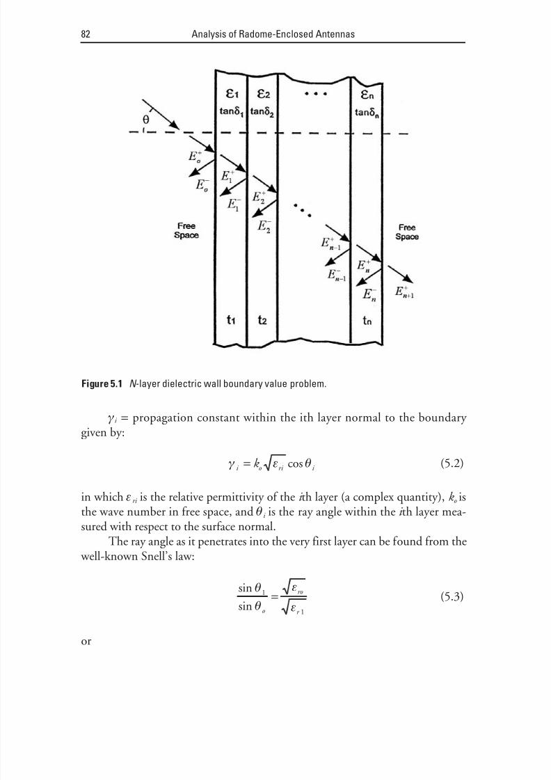
8/20/2019 Analysis of Radome-Enclosed Antennas
http://slidepdf.com/reader/full/analysis-of-radome-enclosed-antennas 103/319

8/20/2019 Analysis of Radome-Enclosed Antennas
http://slidepdf.com/reader/full/analysis-of-radome-enclosed-antennas 104/319
θε
εθ1
1
1
=
−sin sin
ro
r
o (5.4)
Similarly, the angle in each layer can be found from the angle in the previ-ous layer via:
( )θ
ε
εθi
r i
ri
i =
− −
−sin sin1 1
1 (5.5)
Note that the dielectric loss is accounted for by a loss tangent term for thedielectric material:
( )ε ε δri ri j = ′ −1 tan (5.6)
where ′εri is the real part of the relative permittivity for the i th layer. Alternatively one could modify the previous equations to include a conductivity term.
By carrying out the matrix multiplication in (5.1) and gathering termstogether, the equation can then be manipulated to take the form:
E
E
A A
A A
E N 0
0
11 12
21 22
1
0
+
−+
+
=
(5.7)
5.1.1 Transmission Coefficients for Linear Polarization
From (5.7) the final result is obtained for voltage reflection coefficient:
R A
A w =
21
11
(5.8)
Likewise, the transmission voltage coefficient is given by
T A
w = 1
11
(5.9)
Note that both the reflection coefficient and the transmission coefficientare complex and can be expressed in terms of its magnitude and the insertionphase delay (IPD) angle. For instance, the transmission coefficient may beexpressed:
Dielectric Wall Constructions 83

8/20/2019 Analysis of Radome-Enclosed Antennas
http://slidepdf.com/reader/full/analysis-of-radome-enclosed-antennas 105/319
T T IPD w w = ∠ (5.10)
Engineers working in radome design often use the term radome transmis-
sion efficiency for:
T w
2(5.11)
In Appendix 5A a computer software listing is provided for the preceding matrix solution for a multilayer wall transmission coefficient. The software cod-ing was formulated in POWER BASIC [5].
5.1.2 Transmission Coefficients for Circular Polarization
Transmission coefficients for circular polarized waves are computed from thefollowing formulas
T T T T
w copol
w w IPD w IPD
−⊥ ⊥
= − +sin cos∆ ∆
2(5.12)
T T T T
w xpol
w w IPD w IPD
−⊥ ⊥
= − −sin cos∆ ∆2
(5.13)
In whichT w andT w ⊥ = parallel and perpendicular polarization transmission coeffi-cients, respectively;
∆IPD = (IPD ⊥ − IPD w ) = the difference between the perpendicular and theparallel insertion phase delay values.
These co- and cross-polarized transmission coefficient expressions are use-ful to calculate the effects of radome depolarization on antenna performance.
5.1.3 Transmission for Elliptical Polarization
In some cases we transmit or receive a circular polarized signal, but the effect of the polarization is to attenuate or phase delay one of the two orthogonal compo-
nents from the other resulting in the polarization ellipse shown in Figure 5.2.The axial ratio, AR, is defined as the ratio of the magnitudes of the major andminor axes of the polarization ellipse:
AR b
a = (5.14)
84 Analysis of Radome-Enclosed Antennas

8/20/2019 Analysis of Radome-Enclosed Antennas
http://slidepdf.com/reader/full/analysis-of-radome-enclosed-antennas 106/319
or often expressed in decibels
( ) AR AR dB = 20 log (5.15)
Let D be a unit vector perpendicular to the plane defined by the propaga-tion vector and the surface normal in propagating through the radome wall, andletG be a unit vector parallel to the plane defined by the propagation vector andthe surface normal in propagating through the radome wall. A circular polarizedsignal propagating through the radome wall would be modified as:
E T e G T e D t w
jIPD w
jIPD = + ⊥⊥ (5.16)
We can calculate the AR in propagating through the wall by defining:
g T IPD T IPD w w 12
= − +
⊥ ⊥cos sin π
(5.17)
g T IPD T IPD w w 22
= + +
⊥ ⊥sin cos π
(5.18)
g T IPD T IPD w w 3
2= + +
⊥ ⊥cos sin
π(5.19)
g T IPD T IPD w w 4 2= − +
⊥ ⊥sin cos
π
(5.20)
Now let
Dielectric Wall Constructions 85
Figure 5.2 Polarization ellipse.

8/20/2019 Analysis of Radome-Enclosed Antennas
http://slidepdf.com/reader/full/analysis-of-radome-enclosed-antennas 107/319
Y g g = +12
12 (5.21)
Z g g = +32
4
2 (5.22)
From which,
a Y Z
= +
2(5.23)
b Y Z
= − +
2
(5.24)
From which we get the final result:
AR b
a = (5.25)
( ) AR AR dB = 20 log (5.26)
5.2 Radome Types, Classes, and Styles Definition
Radomes for use on flight vehicles (aircraft or missiles), surface vehicles andfixed ground installations are classified into various categories according toMIL-R-7705B [6]. These categories are determined by the specific radome useand wall construction.
There are six types of radomes as identified in the following sections.
5.2.1 Radome Type Definitions
There are six types of radome definitions:
• Type I radomes are low frequency radomes and used at frequencies at orbelow 2.0 GHz.
• Type II radomes are directional guidance radomes having specified
directional accuracy requirements. These include boresight error (BSE),boresight error slope (BSES), antenna pattern distortion, and antenna sidelobe degradation.
• Type III radomes are narrowband radomes with an operational band- width less than 10%.
86 Analysis of Radome-Enclosed Antennas

8/20/2019 Analysis of Radome-Enclosed Antennas
http://slidepdf.com/reader/full/analysis-of-radome-enclosed-antennas 108/319
• Type IV radomes are multiple frequency band radomes used at two ormore narrow frequency bands.
• Type V radomes are broadband radomes generally providing an opera-
tional bandwidth between 0.100 GHz and 0.667 GHz.• Type VI radomes are very broadband radomes that provide an opera-
tional bandwidth greater than 0.667 GHz.
5.2.2 Radome Class Definitions
In addition to the type, the referenced MIL specification defines classes of radomes according to the general application. These are: Class I (flight vehicles),
Class II (surface vehicles), and Class III (fixed ground installations).
5.2.3 Radome Style Definitions
Radome styles are defined according to the dielectric wall construction. Thereare five basic styles described here.
• Style a radomes are half-wave wall solid (monolithic) radomes.
• Style b radomes are thin-wall monolithic structures with a wall thickness
equal to or less than 0.1 λ wavelengths at the highest operating frequency.
• Style c radomes are also called A-sandwich multilayer walls. These con-sist of three layers: two high-density skins and a low-density core mate-rial. The dielectric constant of the skins is greater than the dielectricconstant of the core material.
• Style d radomes are multilayer walled structures having five or moredielectric layers. These have an odd number of high-density skin layersand an even number of low-density core layers. The dielectric constantsof the skins are greater than the dielectric constants of the core materi-als. As the number of layers is increased, the broadband frequency per-formance is improved.
• Style e radomes are defined herein as all possible radome wall construc-tion not fitting into styles a through d. These include the B-sandwichand others. The B-sandwich is similar to the A-sandwich except it con-sists of two low-density skins and a high-density core material. Thedielectric constant of the skins is less than the dielectric constant of thecore material.
Dielectric Wall Constructions 87
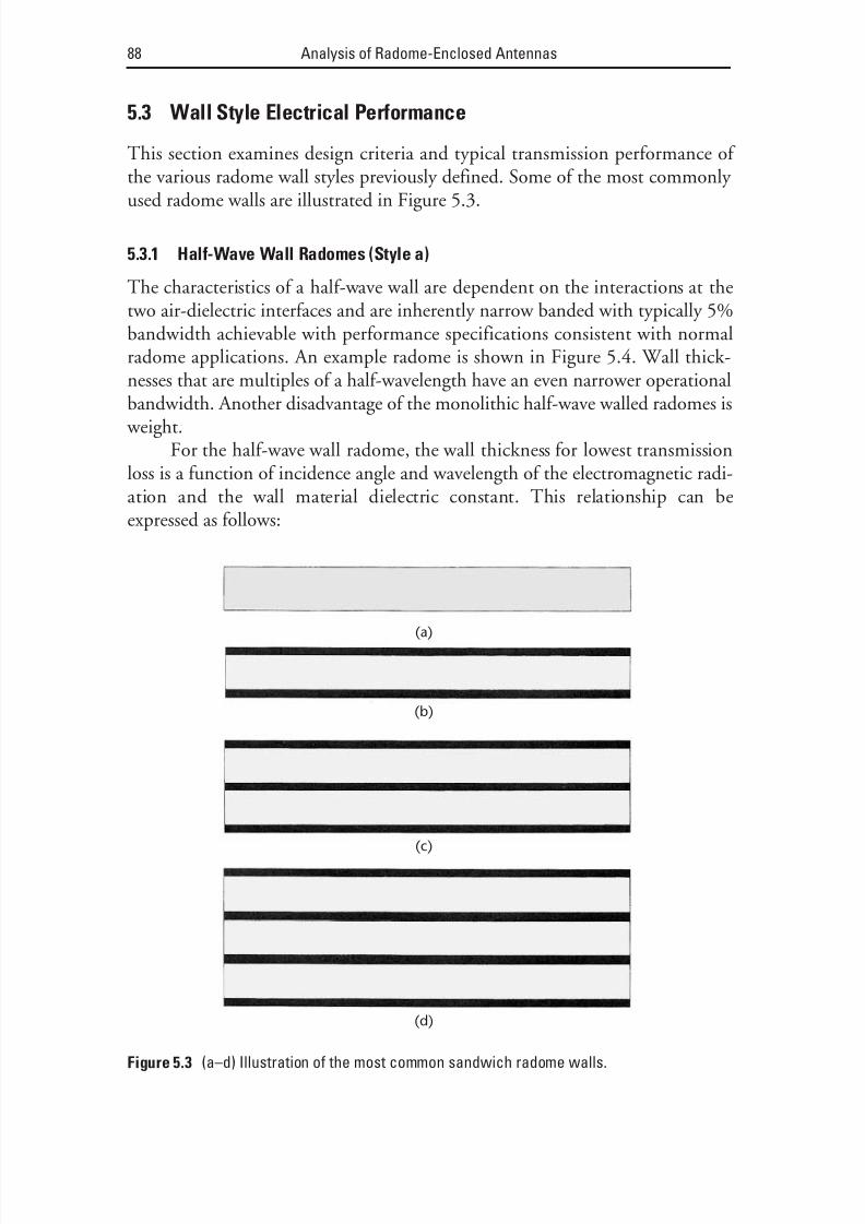
8/20/2019 Analysis of Radome-Enclosed Antennas
http://slidepdf.com/reader/full/analysis-of-radome-enclosed-antennas 109/319
5.3 Wall Style Electrical Performance
This section examines design criteria and typical transmission performance of the various radome wall styles previously defined. Some of the most commonly used radome walls are illustrated in Figure 5.3.
5.3.1 Half-Wave Wall Radomes (Style a)
The characteristics of a half-wave wall are dependent on the interactions at thetwo air-dielectric interfaces and are inherently narrow banded with typically 5%bandwidth achievable with performance specifications consistent with normalradome applications. An example radome is shown in Figure 5.4. Wall thick-
nesses that are multiples of a half-wavelength have an even narrower operationalbandwidth. Another disadvantage of the monolithic half-wave walled radomes is weight.
For the half-wave wall radome, the wall thickness for lowest transmissionloss is a function of incidence angle and wavelength of the electromagnetic radi-ation and the wall material dielectric constant. This relationship can beexpressed as follows:
88 Analysis of Radome-Enclosed Antennas
(d)
(c)
(b)
(a)
Figure 5.3 (a–d) Illustration of the most common sandwich radome walls.

8/20/2019 Analysis of Radome-Enclosed Antennas
http://slidepdf.com/reader/full/analysis-of-radome-enclosed-antennas 110/319
t m
r
=−
λ
ε θ2 2sin(5.27)
Here, λ is the wavelength of radiation and m is the wall order (an integer >= 1).
The voltage transmission coefficient for a monolithic half-wave wall with a thickness of 0.8255 cm is shown in Figures 5.5 and 5.6 for perpendicular andparallel polarizations, respectively. The material had a relative dielectric constantof 4 and a loss tangent of 0.015. The parallel polarization data, in particular,demonstrates zero front face reflection at the Brewster angle given by
( )θ εB = −tan 1 (5.28)
At the Brewster angle, transmission loss through the material is dueentirely to ohmic loss. The loss increases with the increasing value of a materialloss tangent.
The use of multiple half-wave higher-order (i.e., m > 1) wall designs is notnormally considered unless the realization of structural integrity is not possible
Dielectric Wall Constructions 89
Figure 5.4 High performance monolithic radomes in production at British Aerospace. (Photocourtesy of British Aerospace.)

8/20/2019 Analysis of Radome-Enclosed Antennas
http://slidepdf.com/reader/full/analysis-of-radome-enclosed-antennas 111/319
by any other means [7]. The penalties for higher-order monolithic walls arereduced bandwidth and increased radome boresight error (BSE) and radomeboresight error slope (BSES).
90 Analysis of Radome-Enclosed Antennas
Figure 5.5 Half-wave wall transmission, perpendicular polarization (t = 0.8255 cm, εr = 4,
tanδ = 0.015).
Figure 5.6 Half-wave wall transmission, parallel polarization (t = 0.8255 cm, εr = 4, tanδ =0.015).

8/20/2019 Analysis of Radome-Enclosed Antennas
http://slidepdf.com/reader/full/analysis-of-radome-enclosed-antennas 112/319
5.3.2 Thin Walled Radomes (Style b)
The thin wall radome essentially behaves like a lowpass filter below the fre-quency for which it is 0.05 wavelength in thickness [8]. It is particularly useful
for transmission incidence angles ranging from 0° through 70° measured fromthe surface normal [9]. Typical transmission performance data for a material
with relative dielectric constant = 4 and a loss tangent = 0.015 are shown in Fig-ures 5.7 and 5.8 for perpendicular and parallel polarizations, respectively.Often, very thin wall radome structures are implemented as protective coversover telecom antenna apertures as illustrated in Figure 5.9. The thin wallradome finds little aircraft or missile applications above X-band since significantmechanical stresses are to be encountered [10].
5.3.3 A Sandwich Radome (Style c)
An A-sandwich wall consists of two more dense dielectric skins separated by a less dense core having a lower relative dielectric constant than the skins. In air-craft radomes, for instance, A-sandwich constructions generally utilize electri-cally thin plastic skins and cores made of a fiberglass or phenolic honeycomb or
Dielectric Wall Constructions 91
Figure 5.7 Thin wall transmission, perpendicular polarization (εr = 4, tanδ = 0.015).
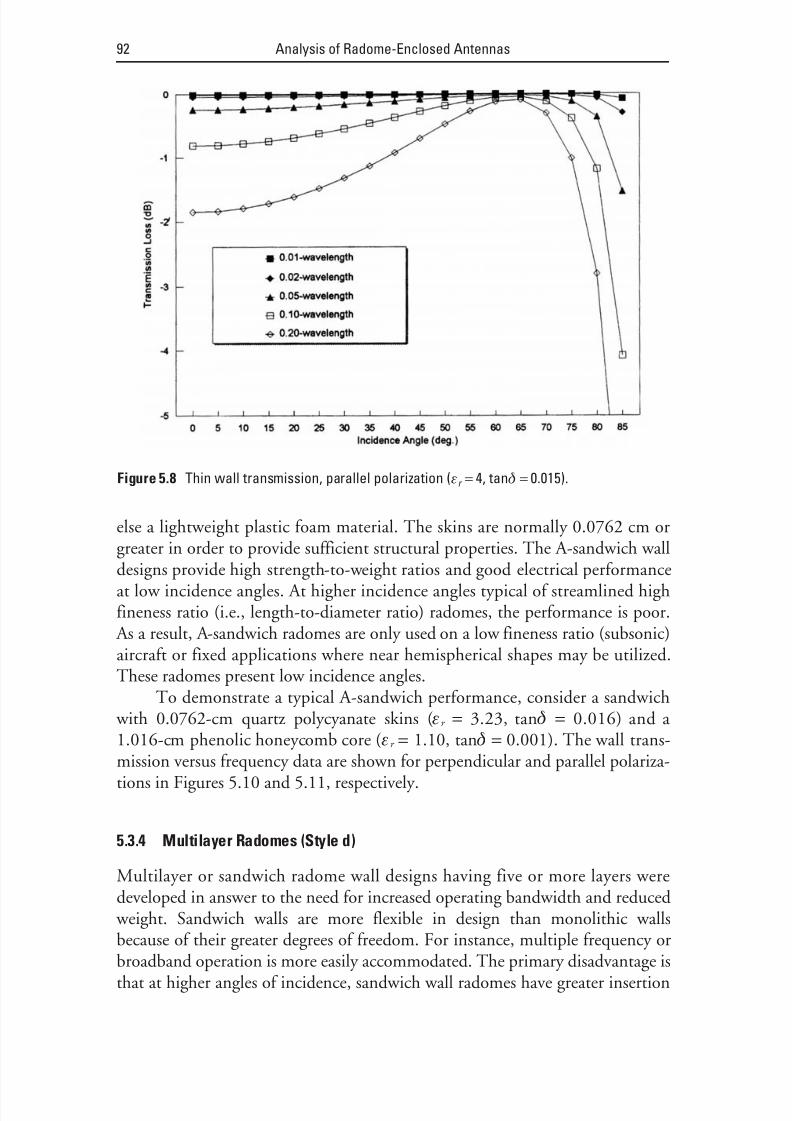
8/20/2019 Analysis of Radome-Enclosed Antennas
http://slidepdf.com/reader/full/analysis-of-radome-enclosed-antennas 113/319
else a lightweight plastic foam material. The skins are normally 0.0762 cm orgreater in order to provide sufficient structural properties. The A-sandwich walldesigns provide high strength-to-weight ratios and good electrical performanceat low incidence angles. At higher incidence angles typical of streamlined highfineness ratio (i.e., length-to-diameter ratio) radomes, the performance is poor.
As a result, A-sandwich radomes are only used on a low fineness ratio (subsonic)aircraft or fixed applications where near hemispherical shapes may be utilized.These radomes present low incidence angles.
To demonstrate a typical A-sandwich performance, consider a sandwich with 0.0762-cm quartz polycyanate skins (εr = 3.23, tanδ = 0.016) and a 1.016-cm phenolic honeycomb core (εr = 1.10, tanδ = 0.001). The wall trans-mission versus frequency data are shown for perpendicular and parallel polariza-tions in Figures 5.10 and 5.11, respectively.
5.3.4 Multilayer Radomes (Style d)
Multilayer or sandwich radome wall designs having five or more layers weredeveloped in answer to the need for increased operating bandwidth and reduced weight. Sandwich walls are more flexible in design than monolithic wallsbecause of their greater degrees of freedom. For instance, multiple frequency orbroadband operation is more easily accommodated. The primary disadvantage isthat at higher angles of incidence, sandwich wall radomes have greater insertion
92 Analysis of Radome-Enclosed Antennas
Figure 5.8 Thin wall transmission, parallel polarization (εr = 4, tanδ = 0.015).

8/20/2019 Analysis of Radome-Enclosed Antennas
http://slidepdf.com/reader/full/analysis-of-radome-enclosed-antennas 114/319
phase delays (IPDs) than monolithic walled radomes. This results in higher BSEand BSES.
The C-sandwich wall consists of a double A-sandwich design. It offers a greater operating bandwidth than the A-sandwich. Also, when properly designed, the C-sandwich provides a reasonably good performance even at ele-vated incidence angles. A representative C-sandwich with 0.0762-cm quartz
Dielectric Wall Constructions 93
Figure 5.9 Photograph of thin wall radome covers over horn antenna apertures. (Photo
courtesy of USDigiComm Corporation.)
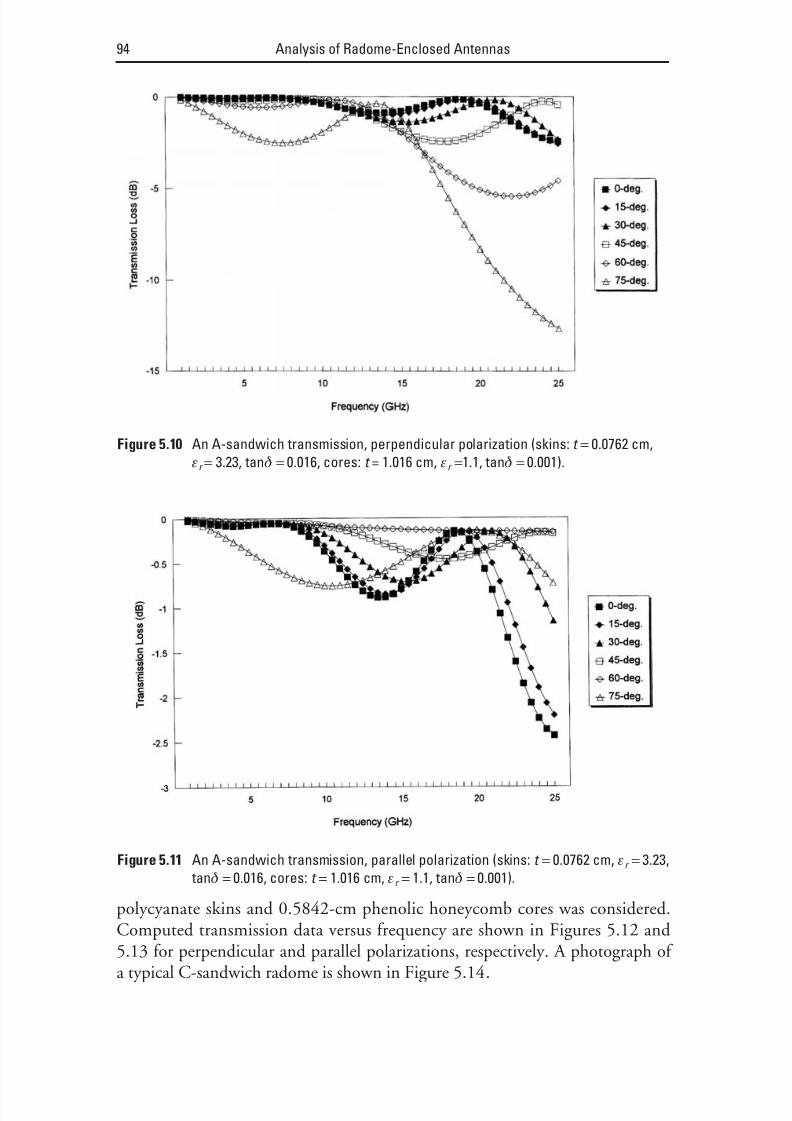
8/20/2019 Analysis of Radome-Enclosed Antennas
http://slidepdf.com/reader/full/analysis-of-radome-enclosed-antennas 115/319
polycyanate skins and 0.5842-cm phenolic honeycomb cores was considered.Computed transmission data versus frequency are shown in Figures 5.12 and5.13 for perpendicular and parallel polarizations, respectively. A photograph of a typical C-sandwich radome is shown in Figure 5.14.
94 Analysis of Radome-Enclosed Antennas
Figure 5.10 An A-sandwich transmission, perpendicular polarization (skins: t = 0.0762 cm,
εr = 3.23, tanδ = 0.016, cores: t = 1.016 cm, εr =1.1, tanδ = 0.001).
Figure 5.11 An A-sandwich transmission, parallel polarization (skins: t = 0.0762 cm, εr = 3.23,
tanδ = 0.016, cores: t = 1.016 cm, εr = 1.1, tanδ = 0.001).

8/20/2019 Analysis of Radome-Enclosed Antennas
http://slidepdf.com/reader/full/analysis-of-radome-enclosed-antennas 116/319

8/20/2019 Analysis of Radome-Enclosed Antennas
http://slidepdf.com/reader/full/analysis-of-radome-enclosed-antennas 117/319
parallel polarizations, respectively. Comparing these data to the previousC-sandwich data, considerable improvement in transmission bandwidth isobserved.
96 Analysis of Radome-Enclosed Antennas
Figure 5.14 Photograph of an experimental broadband C-sandwich radome.
Figure 5.15 Seven-layer wall transmission, perpendicular polarization (skins: t = 0.0762 cm,
εr = 3.23, tanδ = 0.016, cores: t = 0.3302 cm, εr = 1.1, tanδ = 0.001).

8/20/2019 Analysis of Radome-Enclosed Antennas
http://slidepdf.com/reader/full/analysis-of-radome-enclosed-antennas 118/319
5.3.5 B-Sandwich Radomes (Style e)
A B-sandwich wall is similar to the A-sandwich wall. However, it has less densedielectric skins separated by a denser (higher dielectric constant) core. The use of B-sandwich wall radomes have been primarily constrained to terrestrial andmarine applications as opposed to flight vehicles because of structural problemsassociated with low-density dielectric skins such as rain erosion and structuralproblems. In a 1999 patent, MacKenzie [11] considered a multilayer aircraftradome wall design where the outermost layers were low density (with many of
the same physical limitations as the B-sandwich wall discussed here). Such struc-tures were found to exhibit superior broadband performance and millime-ter-wave performance. MacKenzie also invented a retractable radome that couldonly be used on aircraft landing and which might have applications for theB-sandwich as well as his multilayer wall design with low-density outermost skinapplications [12]; structural demands on the radome are minimal at the loweraircraft landing speed.
References
[1] Bodnar, D. G., and H. L. Bassett, “Analysis of an Isotropic Dielectric Radome,” IEEE Transactions on Antennas and Propagation , Vol. AP-23, No. 6, November 1975.
Dielectric Wall Constructions 97
Figure 5.16 Seven-layer wall transmission, parallel polarization (skins: t = 0.0762 cm, εr =3.23, tanδ = 0.016, cores: t = 0.3302 cm, εr = 1.1, tanδ = 0.001).

8/20/2019 Analysis of Radome-Enclosed Antennas
http://slidepdf.com/reader/full/analysis-of-radome-enclosed-antennas 119/319
[2] Yost, D. J., L. B. Weckesser and R. C. Mallalieu, “Technology Survey of Radomes for Anti-Air Missiles,” FS-80-022, John Hopkins Applied Physics Laboratory, Baltimore,MD, 1980.
[3] Collin, R. G., Field Theory of Guided Waves , New York: McGraw-Hill, 1960.
[4] Orfanidis, S. J., “Electromagnetic Waves and Antennas,” Rutgers University, NJ, 2009.
[5] www.powerbasic.com.
[6] Military Specification: General Specification for Radomes , MIL-R-7705 B, January 12,1975.
[7] Tornani, O., Radomes, Advanced Design , North Atlantic Treaty Organization (NATO)Report AGARD-AR-53, prepared by Advisory Group for Aerospace Research and Devel-opment, Neuilly Sur Seine, France, 1973.
[8] Rudge, A. W., G. A. E. Crone, and J. Summers, “Radome Design and Performance,” Con- ference Proceedings of Military Microwaves , IEE (UK), TK6867.C65, 1980.
[9] Cary, R. H. J., “Design of Multi-Band Radomes,” Proceedings of the IEE Conference on Aerospace Antennas (UK) , IEE Publication No. 77, TL694.A6C57, 1971.
[10] Tice, T. E., Techniques for Airborne Radome Design , USAF Report AFATL-TR-66-391,1966.
[11] MacKenzie, B., “Radome Wall Design Having Broadband and Millimeter Wave Charac-teristics,” U.S. Patent 5,408,244, April 1995.
[12] MacKenzie, B., “Retractable. Forward Looking Radome for Aircraft,” U.S. Patent5,969,686, October 1999.
Appendix 5A: Program WALL Computer Software Listing
COMPILE EXE
FUNCTION PBMAIN
‘————————————————————————————————————————————‘GLOBAL VARIABLES NEEDED FOR PROGRAM WALL
GLOBAL wavenumber, ER(), LTAN(), THK(), GAMMA, FREQ, DRAD, Tm(),
Tp() AS DOUBLE
GLOBAL Rtotmag(), Rtotph(), PI AS DOUBLE
GLOBAL N, I, J, K AS INTEGER
DIM ER(1), LTAN(1), THK(1), Tm(2), Tp(2), Rtotmag(2), Rtotph(2)
‘————————————————————————————————————————————
‘ DEFINITION OF INPUT VARIABLES:
‘ N = Number of Layers
‘ THK(i) = Thickness of ith layer (inches)
‘ ER(i) = Relative dielectric constant of ith layer
(dimensionless)
‘ LTAN(i)= Loss tangent of ith layer (dimensionless)
‘ FREQ = frequency (GHz)
‘ GAMMA = angle of incidence (degrees)
‘ DEFINITION OF OUTPUT VARIABLES:
‘ Tm(0) = Magnitude of voltage transmission coefficient (perpen-
dicular polarization)
98 Analysis of Radome-Enclosed Antennas

8/20/2019 Analysis of Radome-Enclosed Antennas
http://slidepdf.com/reader/full/analysis-of-radome-enclosed-antennas 120/319
‘ Tm(1) = Magnitude of voltage transmission coefficient (parallel
polarization)
‘ Tp(0) = Phase of transmission coefficient for perpendicular
polarization (radians)
‘ Tp(1) = Phase of transmission coefficient for parallel polar-
ization (radians)‘ ———————————————————————————————————————————-
DRAD = 3.14159265/180
‘ SAMPLE DATA RUN:
N=3
THK(1)=0.005: ER(1)=3.4: LTAN(1)=.02
THK(2)=0.15: ER(2)=3.58: LTAN(2)=.0045
THK(3)=0.02: ER(3)=3.65: LTAN(3)=0.017
GAMMA=0
FOR FREQ=1 TO 10
wavenumber=0.532*FREQ
GAMMA=GAMMA*DRADGOSUB WALL
PRINT FREQ, Tm(0), Tm(1)
PRINT FREQ, Tp(0)/DRAD, Tp(1)/DRAD
NEXT FREQ
GOTO 1000
‘————————————————————————————————————————
WALL:
‘ THIS SUBROUTINE COMPUTES THE COMPLEX TRANSMISSION COEFFICIENT
THROUGH A MULTI LAYER
LOCAL Am(), Bm(), Cm(), Ap(), Bp(), Cp(), ANG, delay AS DOUBLE
LOCAL IW, JW, KW, POL AS INTEGER
LOCAL R1, R2, E1, E2, R3, E3, tranmag, tranph, SUM, PA, corr AS
DOUBLE
LOCAL ZM(), zph(), rez(), imz(), emag(), eph() AS DOUBLE
LOCAL phimag(), phiph(), rephi(), imphi(), magterm(), angterm()
AS DOUBLE
LOCAL Rmag(), Rph(), reR(), imR(), reT(), imT() AS DOUBLE
LOCAL xx, yy, MAG, ROOTMAG, ROOTANG, NUMMAG AS DOUBLE
LOCAL NUMANG, DENMAG, DENANG AS DOUBLE
DIM Am(10), Bm(10), Cm(10), Ap(10), Bp(10), Cp(10)
DIM ZM(10), zph(10), rez(10), imz(10), emag(10), eph(10)
DIM phimag(10), phiph(10), rephi(10), imphi(10), magterm(10),
angterm(10)DIM Rmag(10), Rph(10), reR(10), imR(10)
DIM Tmag(10), Tph(10), reT(10), imT(10)
FOR POL=0 TO 1
ZM(0) = 1: zph(0) = 0: rez(0) = 1: imz(0) = 0
F O R I W = 1 T O N
xx = ER(IW): yy = ER(IW) * -LTAN(IW)
GOSUB RECTPOLAR
emag(IW) = MAG: eph(IW) = ANG
NEXT IW
rephi(N + 1) = 0: imphi(N + 1) = 0
F O R I W = 1 T O N
xx = ER(IW) - (SIN(GAMMA))^2: yy = ER(IW) * -LTAN(IW)
GOSUB RECTPOLAR
GOSUB COMPLEXSR
magterm(IW) = ROOTMAG: angterm(IW) = ROOTANG
phimag(IW) = wavenumber * magterm(IW)
phiph(IW) = angterm(IW)
MAG = phimag(IW): ANG = phiph(IW)
Dielectric Wall Constructions 99

8/20/2019 Analysis of Radome-Enclosed Antennas
http://slidepdf.com/reader/full/analysis-of-radome-enclosed-antennas 121/319
GOSUB POLARRECT
rephi(IW) = xx: imphi(IW) = yy
zmag(IW) = COS(GAMMA) / (magterm(IW) + 1E-12)
zph(IW) = -angterm(IW)
MAG = zmag(IW): ANG = zph(IW)
GOSUB POLARRECTrez(IW) = xx: imz(IW) = yy
IF POL = 1 THEN
zmag(IW) = 1 / ((emag(IW) * zmag(IW)) + 1E-12)
zph(IW) = -(eph(IW) + zph(IW))
MAG = zmag(IW): ANG = zph(IW)
GOSUB POLARRECT
rez(IW) = xx: imz(IW) = yy
END IF
NEXT IW
zmag(N + 1) = 1: zph(N + 1) = 0
rez(N + 1) = 1: imz(N + 1) = 0F O R I W = 1 T O ( N + 1 )
xx = rez(IW) - rez(IW - 1): yy = imz(IW) - imz(IW - 1)
GOSUB RECTPOLAR
NUMMAG = MAG: NUMANG = ANG
xx = rez(IW) + rez(IW - 1): yy = imz(IW) + imz(IW - 1)
GOSUB RECTPOLAR
DENMAG = MAG: DENANG = ANG
Rmag(IW) = NUMMAG / DENMAG
Rph(IW) = NUMANG - DENANG
MAG = Rmag(IW): ANG = Rph(IW)
GOSUB POLARRECT
reR(IW) = xx: imR(IW) = yy
reT(IW) = 1 + reR(IW): imT(IW) = imR(IW)
xx = reT(IW): yy = imT(IW)
GOSUB RECTPOLAR
Tmag(IW) = MAG: Tph(IW) = ANG
NEXT IW
Am(1) = EXP(-imphi(1) * THK(1))
Am(4) = 1 / Am(1)
Am(2) = Rmag(1) * Am(4)
Am(3) = Rmag(1) * Am(1)
Ap(1) = rephi(1) * THK(1)
Ap(2) = Rph(1) - Ap(1)Ap(3) = Rph(1) + Ap(1)
Ap(4) = -Ap(1)
F O R K W = 2 T O N
Bm(1) = EXP(-imphi(KW) * THK(KW))
Bm(4) = 1 / Bm(1)
Bm(2) = Rmag(KW) * Bm(4)
Bm(3) = Rmag(KW) * Bm(1)
Bp(1) = rephi(KW) * THK(KW)
Bp(2) = Rph(KW) - Bp(1)
Bp(3) = Rph(KW) + Bp(1)
Bp(4) = -Bp(1)
GOSUB CMULT
NEXT KW
Bm(1) = 1: Bm(4) = 1
Bm(2) = Rmag(N + 1): Bm(3) = Bm(2)
Bp(1) = 0: Bp(2) = Rph(N + 1)
Bp(3) = Bp(2): Bp(4) = 0
GOSUB CMULT
100 Analysis of Radome-Enclosed Antennas

8/20/2019 Analysis of Radome-Enclosed Antennas
http://slidepdf.com/reader/full/analysis-of-radome-enclosed-antennas 122/319

8/20/2019 Analysis of Radome-Enclosed Antennas
http://slidepdf.com/reader/full/analysis-of-radome-enclosed-antennas 123/319
END IF
IF (xx > 0) AND (yy < 0) THEN
corr = 0
END IF
IF (xx < 0) AND (yy > 0) THEN
corr = PIEND IF
IF (xx > 0) AND (yy = 0) THEN
corr = 0
END IF
IF (xx < 0) AND (yy = 0) THEN
corr = PI
END IF
IF (xx = 0) AND (yy 0) THEN
corr = 0
END IF
IF (xx = 0) AND (yy = 0) THENANG = 0
END IF
ANG = ATN(yy / (xx + 1E-12)) + corr
RETURN
POLARRECT:
xx = MAG * COS(ANG): yy = MAG * SIN(ANG)
RETURN
COMPLEXSR:
ROOTMAG = SQR(MAG): ROOTANG = ANG / 2
RETURN
101 ‘CONTINUE
‘THE FOLLOWING RETURN IS FOR THE ENTIRE WALL SUBROUTINE
RETURN:
1000 ‘CONTINUE
END FUNCTION
102 Analysis of Radome-Enclosed Antennas
8/20/2019 Analysis of Radome-Enclosed Antennas
http://slidepdf.com/reader/full/analysis-of-radome-enclosed-antennas 124/319
6Radome Analysis Techniques
This chapter summarizes selected radome analysis techniques used to predict a radome-enclosed antenna’s performance. In any analysis technique, the mostsignificant electrical performance parameters of a radome are:
• Boresight error and registration error (if applicable);
• Copolarized and cross-polarized transmission loss;
• Antenna sidelobe-level degradation.
For certain applications, other parameters that might be of concern are theantenna pattern axial ratio (AR) and the antenna voltage standing wave ratio(VSWR) [1].
Ray tracing is a widely used method for describing propagation through a radome wall. When using ray tracing in a receive mode, an incident wavefront is
sampled at uniform sample increments, generally a half-wave apart. From eachof these sample points, a ray in the direction of the propagation vector is tracedthrough the radome wall and onto the antenna aperture where an integration of these rays produces the antenna receive port voltage. The point at which each of these rays intercepts the outer surface of the radome is known as the intercept
point .Ray tracing methods use many approximations, such as the idea of treating
the radome wall at each intercept point as a local plane surface and assuming parallelism between the inner and outer radome walls at the intercept point.Several other factors, such as the antenna size and radome curvature (in wave-lengths), may influence discrepancies between the measured and predicted
103

8/20/2019 Analysis of Radome-Enclosed Antennas
http://slidepdf.com/reader/full/analysis-of-radome-enclosed-antennas 125/319
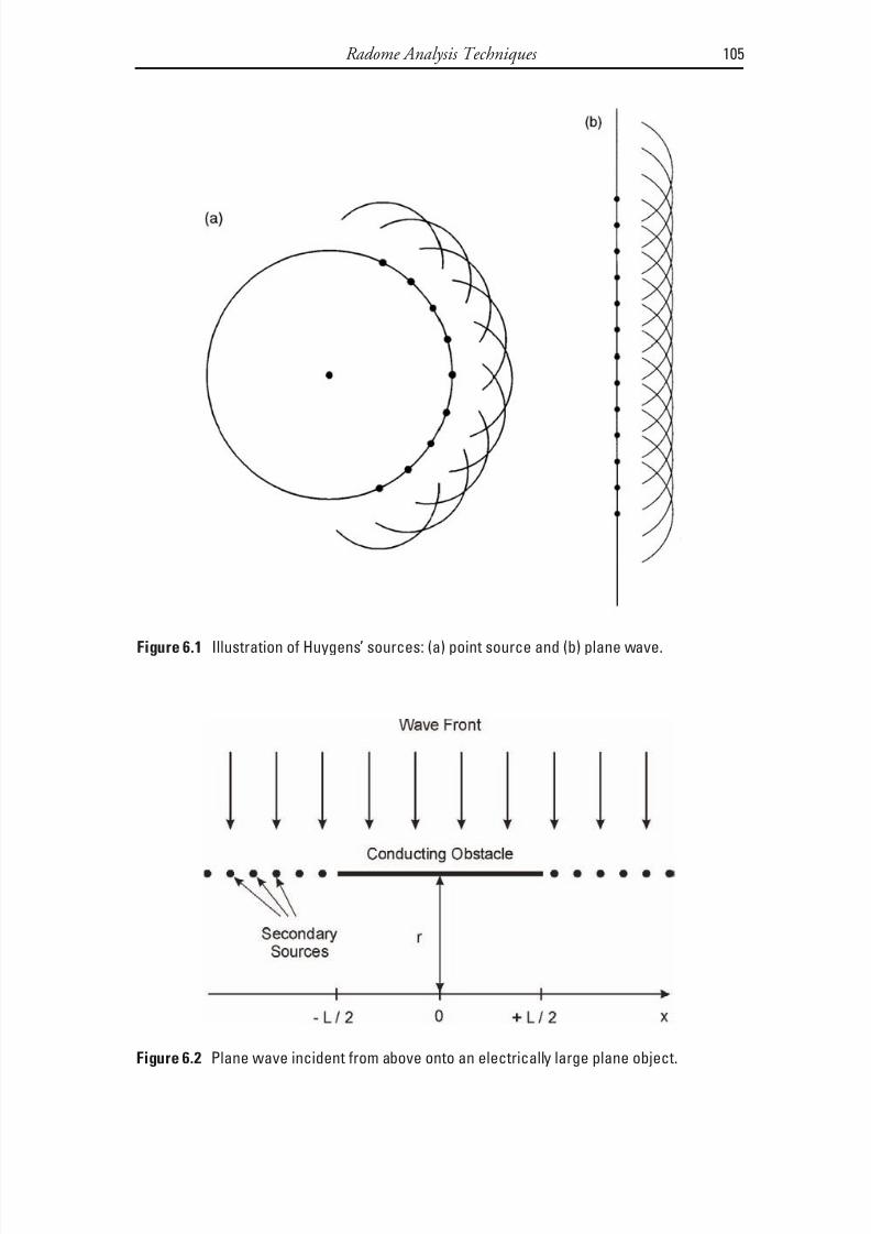
8/20/2019 Analysis of Radome-Enclosed Antennas
http://slidepdf.com/reader/full/analysis-of-radome-enclosed-antennas 126/319
Radome Analysis Techniques 105
Figure 6.1 Illustration of Huygens’ sources: (a) point source and (b) plane wave.
Figure 6.2 Plane wave incident from above onto an electrically large plane object.

8/20/2019 Analysis of Radome-Enclosed Antennas
http://slidepdf.com/reader/full/analysis-of-radome-enclosed-antennas 127/319
E dE i = ∫ (6.1)
where dE is the electric field at point P and the integration is along the x -axis as
illustrated in Figure 6.2. We note that in terms of the wave number k , the fol-lowing holds true:
( )dE E
r e dx o k r = − + δ (6.2)
so that
E E r
e e dx i o jkr jk = − −
− ∞
∞∫ δ (6.3)
The PO solution for the power density variation at a distance r below theplane is shown in Figure 6.3. Also depicted is the GO solution wherein it is seenthat the conducting obstacle casts a simple shadow, illustrating its light-likebehavior. Intuitively, the PO approach is more robust. For instance, assume anincident wavefront on a radome having a conducting rain erosion tip. The GOmodeling approach would cast a simple tip shadow onto the antenna aperture.The PO modeling approach is more robust in predicting the actual electromag-netic (EM) fields incident on the antenna aperture.
Section 6.2 discusses the geometric optics method applied by Kilcoyne todevelop a two-dimensional ray tracing code for analyzing radomes on a digitalcomputer [10]. Bagby subsequently published a three-dimensional GO methodapplicable to the desktop computer–aided design of aircraft radomes [11].
106 Analysis of Radome-Enclosed Antennas
Figure 6.3 Power density variation for the plane wave incident from above onto an electri-
cally large plane object.

8/20/2019 Analysis of Radome-Enclosed Antennas
http://slidepdf.com/reader/full/analysis-of-radome-enclosed-antennas 128/319

8/20/2019 Analysis of Radome-Enclosed Antennas
http://slidepdf.com/reader/full/analysis-of-radome-enclosed-antennas 129/319
solution for a three-dimensional cone was reported by Mahan and Bone [24].Both considered a monolithic radome wall and the approach-traced rays froman incident wavefront through the radome walls onto an internal antenna aper-
ture assuming that the refraction effects at the air-dielectric boundaries can bedescribed by Snell’s law. Another early GO transmit formulation modeled the antenna aperture as a
collection of sources with arbitrary amplitude and phase. The collection of raysdefined an equivalent aperture outside of the radome whose amplitude andphase distributions incorporated the effect of the radome [25]. The Fouriertransform of this distribution yielded the far-field radiation pattern of theradome-enclosed antenna. In Einziger and Felson [26], GO ray tracing alsoaccounted for multiple reflections on the concave (inner) radome side and for
reflections between its layer boundaries.
6.2.1 GO Receive Mode Calculations
The receiving formulation finds the voltage at the antenna port when a plane wave is incident on a radome-enclosed antenna, as illustrated in Figure 6.4(a).This is sometimes referred to as a backward ray trace . The antenna receive port
voltage is obtained from the incident fields and the known characteristics of theantenna. Thus, the problem is really one of finding the incident fields at theantenna in the presence of both the radome and the antenna [27]. Formonopulse radar antennas, we can derive a quantitative estimate of the radomeboresight error from the complex sum and difference antenna patterns com-puted without and with the radome in place.
Assume an incident plane EM wave coming from an arbitrary but fixeddirection, θ and ϕ. To obtain the received antenna voltage, we integrate the
wavefront data over the receive antenna aperture in accordance with the equiva-lence theorem [6]. This leads to a calculation of the propagation of the EM fieldto its values on the antenna aperture surface. Accordingly, the received complex voltage at the terminal of the antenna is [13, 28]:
( )F E T da a i w ∫ ∫ (6.4)
This integration extends over the physical antenna surface area for which
F
a
has a significant contribution. In addition, E
i
is the incident plane wave func-tion, F a is the complex valued receiving aperture distribution at point on theantenna surface, and T W is the complex valued radome transmission coefficient a ray intercept point.
Usually, the radome is treated as a local plane at each ray intercept point[29], which leads to small errors in the calculation of T W . The transmission
108 Analysis of Radome-Enclosed Antennas

8/20/2019 Analysis of Radome-Enclosed Antennas
http://slidepdf.com/reader/full/analysis-of-radome-enclosed-antennas 130/319

8/20/2019 Analysis of Radome-Enclosed Antennas
http://slidepdf.com/reader/full/analysis-of-radome-enclosed-antennas 131/319
The antenna aperture distribution, F a , can be found from probing thenear field at several wavelengths from an actual antenna surface and applying a backward propagation (Fourier transform) technique [12]. Alternatively, it can
be probed very close to the antenna aperture with a suitable probe.
6.2.2 GO Transmit Mode Calculations
The transmit mode is illustrated in Figure 6.4(b). The antenna aperture distri-bution is projected through the radome wall to form an equivalent aperture out-side of the radome. However, each ray is modified by the amplitude and phaseof its associated radome transmission coefficients, and the modified effective
aperture distribution includes the effect of the radome walls. Thus, points form-ing the modified aperture distribution are related to the actual aperturedistribution via:
F T F mn a
w mn a ′ = (6.5)
where F mn is the complex valued transmit aperture distribution at the point onthe actual antenna aperture and T W is the complex valued radome transmission
coefficient associated with the intercept of the mn th ray at its intercept point. Inthis case, the equivalent aperture size is identical in size to the actual antenna aperture. Assume that the antenna is in the x - y plane with the z -coordinate cor-responding to the radome axis. We can obtain the far-field antenna array patternfrom the reference plane distribution by applying the following formula.
( )E F e t mn a
n
N
m
M jk x y m n = ′
==
− +∑∑11
sin cos sin sinθ φ θ φ (6.6)
where x m = m d x , y n = n d y ,and d x , d y are the sample spacing in x- and y -coordinatedirections, respectively.
6.3 Physical Optics (PO) Approaches
In analyzing the performance of a radome-enclosed antenna system, physical
optics techniques generally offer a higher computational accuracy than geomet-ric optics, due to the assumptions of geometric optics. For instance, GO makesthe assumption that the EM wave propagates as a plane wave confined to a cyl-inder whose cross section the antenna aperture defines. However, in reality thefield diverges. Shifflett [31] gives a good overview of the method. In the follow-ing sections we attempt to explain some of the variants of PO radome analysis.
110 Analysis of Radome-Enclosed Antennas
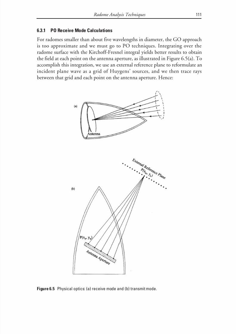
8/20/2019 Analysis of Radome-Enclosed Antennas
http://slidepdf.com/reader/full/analysis-of-radome-enclosed-antennas 132/319
6.3.1 PO Receive Mode Calculations
For radomes smaller than about five wavelengths in diameter, the GO approachis too approximate and we must go to PO techniques. Integrating over the
radome surface with the Kirchoff-Fresnel integral yields better results to obtainthe field at each point on the antenna aperture, as illustrated in Figure 6.5(a). Toaccomplish this integration, we use an external reference plane to reformulate anincident plane wave as a grid of Huygens’ sources, and we then trace raysbetween that grid and each point on the antenna aperture. Hence:
Radome Analysis Techniques 111
Figure 6.5 Physical optics: (a) receive mode and (b) transmit mode.
8/20/2019 Analysis of Radome-Enclosed Antennas
http://slidepdf.com/reader/full/analysis-of-radome-enclosed-antennas 133/319
V F E T e
r ds da a
a i w
jkr
=
∫∫ ∫∫
−
(6.7)
The outer integration extends over the antenna surface area for which F a
has a significant contribution, and the inner integration is over the external ref-erence plane where:
E i = incident plane wave function;
F a = complex valued receiving aperture distribution at a point on the an-tenna surface;
T W = complex valued radome transmission coefficient at a ray intercept
point;k = wave number = 2 π/ λ;
r = the distance from each point on the external reference plane to an an-tenna aperture point, x a , y a , z a .
The direct ray (GO) and surface integration (PO) methods differ primar-ily in the computation of the total transmission coefficient. With the POmethod, the integration of a bundle of rays through the radome wall, as opposedto a single ray, more densely samples the curvature variation results in a more
robust wall transmission model. Both methods use the flat panel approximationto compute wall transmission coefficients at the ray intercept points and ignoreboth multiple internal reflections and trapped waves. Hayward et al. [12] havecompared predicted with measured data for these two receive ray trace methods.Overall, the researchers found that the surface integration was more accurate,especially for radomes that were small in wavelengths.
6.3.2 PO Transmit Mode Calculations
In a physical optics transmit formulation, the following steps occur, which con-form better to reality:
• We obtain the antenna near-field distribution on the inner radomesurface.
• The transmission coefficients of the radome wall are applied to give thefield on the exterior of the radome.
• We make a final transformation to the far field by a Fourier transformtechnique.
A useful radome analysis technique researched by Raz et al. [14] and Israelet al. [15] uses PO for tracing the field from an antenna aperture through the
112 Analysis of Radome-Enclosed Antennas

8/20/2019 Analysis of Radome-Enclosed Antennas
http://slidepdf.com/reader/full/analysis-of-radome-enclosed-antennas 134/319
radome wall to an external reference plane, where contributions are collected.The geometry is illustrated in Figure 6.5(b).
Assuming that each point on the antenna aperture radiates as a Huygens’
source, the complex distribution can be derived for each point on an externalreference plane via:
F F T e
r da mn
a a w
jkr ′
−
= ∫∫ (6.8)
The integration extends over the physical antenna surface area for whichF a has significant contribution and where
F mn
a ′
= complex valued transmit aperture distribution at a point on the ex-ternal reference plane surface;
T W = complex valued radome transmission coefficient at ray intercept
point;
k = wave number = 2 π/ λ;
r = the distance from each point on the antenna aperture to a point x m , y
n
on the external reference plane.
Here the area forming the external reference plane should be larger thanthe physical area of the radome-enclosed antenna. An exact solution correspondsto an infinite external plane, but this is not possible. Typically, we may take ittwo to four times the physical area of the antenna. The far-field antenna array pattern can be computed from the reference plane distribution as we did in(6.6).
( )E F e t mn a
n
N
m
M jk x y m n = ′
==
− +∑∑11
sin cos sin sinθ φ θ φ (6.9)
where x m = m d x , y n = n d y ,and d x , d y are the sample spacings in x -and y -coordi-nate directions, respectively.
6.4 Other Approaches
6.4.1 Method of Moments (MOM)
Joy et al. [20] applied a two-dimensional method of moments technique to a tangent ogive radome based on the approach developed by Richmond [28–30].
An integral equation for the electric field was solved by dividing the dielectricinto cells that were small enough so that the electric field intensity was approxi-mately uniform in each cell.
Radome Analysis Techniques 113

8/20/2019 Analysis of Radome-Enclosed Antennas
http://slidepdf.com/reader/full/analysis-of-radome-enclosed-antennas 135/319
Also applying a MOM approach, Tricoles, Rope, and Hayward [32] ana-lyzed the EM fields scattered by a hollow cone, using two formulations. One
was based on a scalar Green’s function and the other on a tensor Green’s func-
tion. The two are equivalent, but the procedures differ in the following ways.
• The scalar Green’s function method decomposes the cone into circularcylinders and subsequently decomposes the cylinders into angular sec-tors. The tensor Green’s function method decomposes the cone intospheres.
• The number of cells differs because the cell sizes differ.
• Polarization dependence differs.
Tricoles et al. [15] applied this MOM technique to dielectric cylinders of an arbitrary shape. Although sophisticated, the MOM is more difficult to apply to radome modeling than the other methods previously discussed. Very limitedvalidation data appears in the technical literature to compare its accuracy with
geometric optics of physical optics methods. However, MOM may give theeffects of guided waves or scattering by a radome rain erosion tip.In 2001, Abdel Moneum et al. [33] developed a hybrid technique for elec-
trically large axisymmetric tangent ogive shaped radomes. The method appliesMOM analysis for the wall in the nose region and PO analysis for the remaining
wall.
6.4.2 Plane Wave Spectra (PWS)
Paris developed a three-dimensional approach that could find the tangentialfields on the outside radome surface due to a horn antenna radiating inside theradome [16]. Wu and Rudduck developed a three-dimensional method thatused a plane wave spectrum representation to characterize the antenna [17]. A discrete PWS is a complex vector array obtained from a Fourier transform of thenear-field aperture field and represents the radiating antenna properties. If anantenna aperture has M by N sample points, then the PWS contains MN plane
waves. The approach is illustrated in Figure 6.6. Joy and Huddleston expanded on this idea by using a fast Fourier trans-form (FFT) to speed up the computer calculations when applying a plane wavespectrum approach [18]. PWS is believed to give more accurate results thaneither the GO or PO approaches discussed earlier. However, PWS requires a considerably greater computer run time and cannot be implemented on a PC.
114 Analysis of Radome-Enclosed Antennas

8/20/2019 Analysis of Radome-Enclosed Antennas
http://slidepdf.com/reader/full/analysis-of-radome-enclosed-antennas 136/319
6.4.3 FDTD and Integral Equation Methods
A method for solving the differential form of Maxwell’s equations is known asthe finite-difference time-domain (FDTD) method. Maloney and Smith [34]present methodology to apply FDTD to model a radome. The method requiresdefining a grid over the radome and surrounding space and then applying boundary conditions. The technique can be computationally intensive com-pared to the ray trace methods discussed in this chapter.
For a radome that is large in terms of wavelengths, integral equation meth-ods are also generally impractical because of the enormous computationalrequirements. However, applying the technique to a two dimensional geometry greatly reduces the computer run time. In [35] Sukharevsky et al. reported onthe successful application of the technique to a large fineness ratiotwo-dimensional radome.
6.5 Sources of Computational Error
Ray trace computational errors have several causes, including:
• Antenna modeling;
• Statistical wall variations;
Radome Analysis Techniques 115
Figure 6.6 Illustration of a plane wave spectra (PWS) approach.
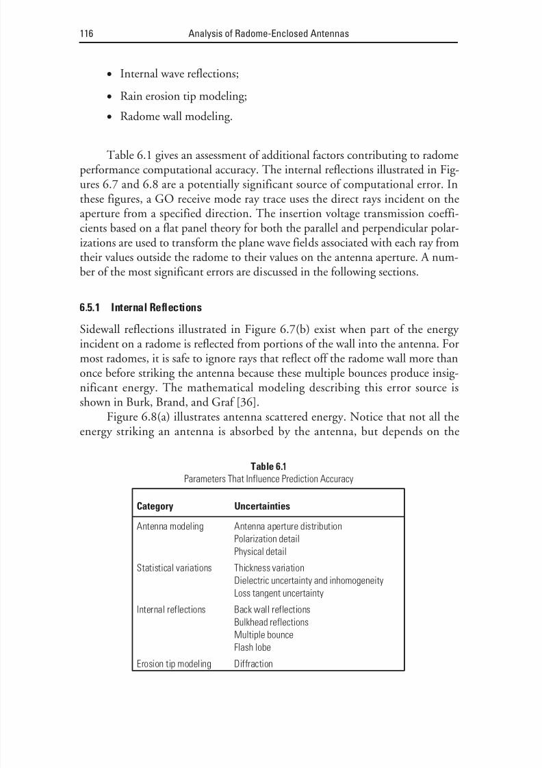
8/20/2019 Analysis of Radome-Enclosed Antennas
http://slidepdf.com/reader/full/analysis-of-radome-enclosed-antennas 137/319
• Internal wave reflections;
• Rain erosion tip modeling;
• Radome wall modeling.
Table 6.1 gives an assessment of additional factors contributing to radomeperformance computational accuracy. The internal reflections illustrated in Fig-ures 6.7 and 6.8 are a potentially significant source of computational error. Inthese figures, a GO receive mode ray trace uses the direct rays incident on theaperture from a specified direction. The insertion voltage transmission coeffi-cients based on a flat panel theory for both the parallel and perpendicular polar-
izations are used to transform the plane wave fields associated with each ray fromtheir values outside the radome to their values on the antenna aperture. A num-ber of the most significant errors are discussed in the following sections.
6.5.1 Internal Reflections
Sidewall reflections illustrated in Figure 6.7(b) exist when part of the energy incident on a radome is reflected from portions of the wall into the antenna. For
most radomes, it is safe to ignore rays that reflect off the radome wall more thanonce before striking the antenna because these multiple bounces produce insig-nificant energy. The mathematical modeling describing this error source isshown in Burk, Brand, and Graf [36].
Figure 6.8(a) illustrates antenna scattered energy. Notice that not all theenergy striking an antenna is absorbed by the antenna, but depends on the
116 Analysis of Radome-Enclosed Antennas
Table 6.1
Parameters That Influence Prediction Accuracy
Category Uncertainties
Antenna modeling Antenna aperture distribution
Polarization detail
Physical detail
Statistical variations Thickness variation
Dielectric uncertainty and inhomogeneity
Loss tangent uncertainty
Internal reflections Back wall reflections
Bulkhead reflections
Multiple bounce
Flash lobe
Erosion tip modeling Diffraction

8/20/2019 Analysis of Radome-Enclosed Antennas
http://slidepdf.com/reader/full/analysis-of-radome-enclosed-antennas 138/319
antenna’s aperture distribution. The inverse of the antenna’s illumination func-tion often provides an approximation to the energy reflected by the antenna aperture. The antenna scattered energy can bounce off the radome wall one ormore times before striking the antenna. Again, rays that reflect off the radome
wall more than once before striking the antenna are relatively small and can beignored.
Many aircraft or missiles have a bulkhead plate between the radome andthe vehicle body, as illustrated in Figure 6.8(b). If this bulkhead is not micro-
wave-absorber treated, incoming rays can reflect off this surface and strike thebackside of the antenna. The backlobe pattern of the antenna receives the bulk-head reflected energy causing boresight errors. Generally, bulkhead reflections
will not have much effect until the angle of incidence of the incoming rays (withrespect to the radome axis) becomes large. In actual applications, positioners and
Radome Analysis Techniques 117
(b)
(a)
Figure 6.7 Internal ray reflections: (a) no reflections and (b) sidewall reflections.

8/20/2019 Analysis of Radome-Enclosed Antennas
http://slidepdf.com/reader/full/analysis-of-radome-enclosed-antennas 139/319
other electronic hardware may block some reflections from reaching theantenna.
To evaluate the typical contribution of each of the ray bounce error contri-butors, we studied an A-sandwich tangent ogive radome with a fineness ratio of
3. The antenna size was approximately 20 wavelengths at the operating fre-quency and the polarization was vertical. Using a GO receive mode predictionmodel, we compared the measured elevation plane boresight error (BSE) data topredicted data in Figure 6.9. For this particular radome, when ignoring all inter-nal reflection error sources, there was reasonably good correlation between
118 Analysis of Radome-Enclosed Antennas
(b)
(a)
Figure 6.8 Internal ray reflections: (a) antenna scattered energy and (b) bulkhead
reflections.
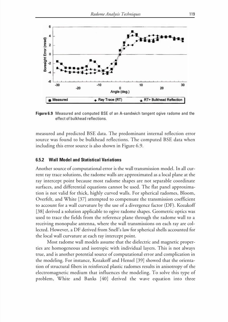
8/20/2019 Analysis of Radome-Enclosed Antennas
http://slidepdf.com/reader/full/analysis-of-radome-enclosed-antennas 140/319
measured and predicted BSE data. The predominant internal reflection errorsource was found to be bulkhead reflections. The computed BSE data whenincluding this error source is also shown in Figure 6.9.
6.5.2 Wall Model and Statistical Variations
Another source of computational error is the wall transmission model. In all cur-rent ray trace solutions, the radome walls are approximated as a local plane at theray intercept point because most radome shapes are not separable coordinatesurfaces, and differential equations cannot be used. The flat panel approxima-tion is not valid for thick, highly curved walls. For spherical radomes, Bloom,Overfelt, and White [37] attempted to compensate the transmission coefficientto account for a wall curvature by the use of a divergence factor (DF). Kozakoff [38] derived a solution applicable to ogive radome shapes. Geometric optics wasused to trace the fields from the reference plane through the radome wall to a receiving monopulse antenna, where the wall transmissions on each ray are col-lected. However, a DF derived from Snell’s law for spherical shells accounted forthe local wall curvature at each ray intercept point.
Most radome wall models assume that the dielectric and magnetic proper-ties are homogeneous and isotropic with individual layers. This is not always
true, and is another potential source of computational error and complication inthe modeling. For instance, Kozakoff and Hensel [39] showed that the orienta-tion of structural fibers in reinforced plastic radomes results in anisotropy of theelectromagnetic medium that influences the modeling. To solve this type of problem, White and Banks [40] derived the wave equation into three
Radome Analysis Techniques 119
Figure 6.9 Measured and computed BSE of an A-sandwich tangent ogive radome and the
effect of bulkhead reflections.

8/20/2019 Analysis of Radome-Enclosed Antennas
http://slidepdf.com/reader/full/analysis-of-radome-enclosed-antennas 141/319
components to deal with a plane wave transmission and reflection fromanisotropic materials. Guided waves were observed to propagate in radome wallsby Tricoles [41] and are a potential source of computational error.
According to Ersoy and Ford [42], a radome performance degradationfrom the theoretical predictions also occurs from radome surface irregularities.Vorobyev [43] has applied statistical methods to manufacturing tolerances (onboth the dielectric constant and the wall thickness) and related the manufactur-ing tolerances to the electrical performance of radomes.
References
[1] Torani, O., Radomes, Advanced Design , AGARD Advisory Report No. 53, Advisory Groupfor Aerospace Research and Development, North Atlantic Treaty Organization (NATO),Neuilly Sur Seine, France, 1953, pp. 111–112.
[2] Kaplun, V. A., “Nomographs for Determining the Parameters of Plane Dielectric Layersof Various Structure with Optimum Radio Characteristics,” Radiotechnika i Electronika (USSR), Part 2, Vol. 20, No. 9, 1975, pp. 81–88.
[3] Zamyatin, V. I., A. S. Klyuchnikov, and V. I. Shvets, Antenna Fairings , Minsk, USSR: V.I. Lenin Belorussian Publishing House, 1980.
[4] Kaplun, V. A., and V. M. Zelenkevich, “Introduction to Computer-Aided Design of Microwave Antenna Radomes,” Radiotechnika i Electronika (USSR), Vol. 42, No. 2, 1987,pp. 89–93.
[5] Mahan, A. I., C. V. Bitterli, and C. G. Wein, “Far Field Diffraction and Boresight ErrorProperties of a Two Dimensional Wedge,” Journal of the Optical Society of America , Vol.49, No. 6, June 1959, pp. 535–566.
[6] Tricoles, G., “Radiation Patterns and Boresight Error of a Microwave Antenna Enclosedin an Axially Symmetric Dielectric Shell,” Journal of the Optical Society of America , Vol. 54,No. 9, September 1964, pp. 1094–1101.
[7] Tricoles, G., “Radiation Patterns of a Microwave Antenna Enclosed in a Hollow Dielec-tric Wedge,” Journal of the Optical Society of America , Vol. 53, No. 5, May 1963, pp.545–557.
[8] Milligan, T. A., Modern Antenna Design , New York: McGraw-Hill, 1985, pp. 215–216.
[9] Kraus, J. D., Antennas , 2nd ed., New York: McGraw-Hill, 1988, pp. 174–189.
[10] Kilcoyne, N. R., “An Approximate Calculation of Radome Boresight Error,” Proceedings of the USAF/Georgia Institute of Technology Symposium on Electromagnetic Windows , Georgia
Institute of Technology, Atlanta, GA, June 1968, pp. 91–111.
[11] Bagby, J., “Desktop Computer Aided Design of Aircraft Radomes,” IEEE MIDCON 88 Conference Record , Western Periodicals Company, North Hollywood, CA, 1988, pp.258–261.
120 Analysis of Radome-Enclosed Antennas

8/20/2019 Analysis of Radome-Enclosed Antennas
http://slidepdf.com/reader/full/analysis-of-radome-enclosed-antennas 142/319
[12] Hayward, R. A., E. L. Rope, and G. Tricoles, “Accuracy of Two Methods for Numerical Analysis of Radome Electromagnetic Effects,” Proceedings of the 14th Symposium on Elec- tromagnetic Windows , Georgia Institute of Technology, Atlanta, GA, 1978, pp. 53–57.
[13] Hayward, R. A., E. L. Rope, and G. Tricoles, “Accuracy of Two Methods for Numerical Analysis of Radome Electromagnetic Effects,” IEEE International Symposium Digest on Antennas and Propagation , Seattle, WA, June 1979, pp. 598–601.
[14] Raz, S., et al., “Numerical Analysis of Antenna Radome Systems,” Proceedings of the 10th IEEE Convention , Tel Aviv, Israel, October 1977.
[15] Israel, M., et al., “A Reference Plane Method for Antenna Radome Analysis,” Proceedings of the 15th Symposium on Electromagnetic Windows , Georgia Institute of Technology,
Atlanta, GA, 1980, pp. 34–39.
[16] Tricoles, G., E. L. Rope, and R. A. Hayward, “Analysis of Radomes by the Method of Moments Method,” Proceedings of the 17th Symposium on Electromagnetic Windows , Geor-gia Institute of Technology, Atlanta, GA, 1984, pp. 1–8.
[17] Wu, D. C. F., and R. C. Rudduck, “Plane Wave Spectrum Surface Integration Techniquefor Radome Analysis,” IEEE Transactions on Antennas and Propagation , AP-22, No.3, May 1974, pp. 497–500.
[18] Joy, E. B., and G. K. Huddleston, Radome Effects on Ground Mapping Radar , Final Reporton Contract DAAH01-72-C-0598, SF-778 203/0, U.S. Army Missile Command,Huntsville, AL, May 1973.
[19] Huddleston, G. K., H. L. Bassett, and J. M. Newton, Parametric Investigation of Radome Analysis Methods; Computer Aided Radome Analysis Using Geometric Optics and Lorentz Rec- iprocity , Final Report on Contract AFOSR-77-3469, Volumes 1-3, Georgia Institute of Technology, Atlanta, GA, 1981.
[20] Joy, E. B., et al., “Comparison of Radome Electrical Analysis Techniques,” Proceedings of the 15th Symposium on Electromagnetic Windows , Georgia Institute of Technology, Atlanta,GA, 1980, pp. 29–33.
[21] Tavis, M., A Three-Dimensional Ray Tracing Method for Calculation of Radome Boresight
Error and Antenna Pattern Distortion , Aerospace Corporation Report, TOR-0059(56860), AD 729811, 1971.
[22] Einziger, P. D., and L. B. Felson, “Ray Analysis of Two-Dimensional Radomes,” IEEE Transactions on Antennas and Propagation , Vol. AP-31, No. 6, 1983, pp. 870–884.
[23] Deschamps, G. A., “Ray Techniques in Electromagnetics,” Proceedings of the IEEE , Vol.60, No. 9, September 1972, pp. 1021–1035.
[24] Mahan, A. I., and L. P. Bone, “Far Field Diffraction and Polarization Properties of a Three Dimensional Hollow, Homogeneous, Isotropic Cone,” Journal of the Optical Society of America , Vol. 53, No. 5, May 1963, pp. 533–544.
[25] Hayward, R. A., and G. P. Tricoles, “Radome Boresight Error: Numerical Prediction andPhysical Interpretation,” IEEE Antennas and Propagation Society (AP-S) Digest , IEEE Cata-log No. 75CH0963-9AP, June 1975, pp. 61–63.
Radome Analysis Techniques 121

8/20/2019 Analysis of Radome-Enclosed Antennas
http://slidepdf.com/reader/full/analysis-of-radome-enclosed-antennas 143/319
[26] Einziger, P. D., and L. B. Felsen, “Rigorous Asymptotic Analysis of TransmissionThrough a Curved Dielectric Slab,” IEEE Transactions on Antennas and Propagation , Vol.
AP-31, No. 6, November 1983, pp. 863–869.
[27] Richmond, J. H., “Scattering by Dielectric Cylinders of Arbitrary Cross Sectional Shapes,”IEEE Transactions on Antennas and Propagation , Vol. AP-13, 1965, pp. 334–341.
[28] Richmond, J. H., The Calculation of Radome Diffraction Patterns , Ohio State University,Department of Electrical Engineering Report 1180-13, AD-423660 September 1966.
[29] Richmond, J. H., “TE Wave Scattering by a Dielectric Cylinder of Arbitrary Cross Sec-tional Shape,” IEEE Transactions on Antennas and Propagation , Vol. AP-14, 1966, pp.460–464.
[30] Tricoles, G., E. L. Rope, and R. A. Hayward, Wave Propagation Through Axially Symmetric Missile Radomes , Final Report No. R-81-125 on Contract N00019-79-C-0638,
AD-A106762/8, 1981.
[31] Shifflett, J. A., CADDRA: A Physical Optics Radar Radome Analysis Code for Arbitrary 3D Geometries,” IEEE Antennas and Propagation Magazine , Vol. 39, No. 6, 1977, pp.73–79.
[32] Paris, D. T., “Computer Aided Radome Analysis,” IEEE Transactions on Antennas and Propagation , Vol. AP-18, No. 1, January 1970, pp. 7–15.
[33] Abdel Moneum, M. A., et al., “Hybrid PO-MOM Analysis of Large Axi-SymmetricRadomes,” IEEE Transactions on Antennas and Propagation , Vol. 49, No. 12, 2001, pp.
1657–1660.
[34] Maloney, J. G., and G. S. Smith, “Modeling of Antennas,” in Advances in Computational Electrodynamics , A. Taflove, (ed.), Norwood, MA: Artech House, 1998, pp. 453–456.
[35] Sukharevsky, O. I., S. V. Kukobko, and A. Z. Sazonov, “Volume Integral Equation Analy-sis of a Two Dimensional Radome with a Sharp Nose,” IEEE Transactions and Propaga- tion , Vol. 53, No. 4, 2005, pp. 1500–1506.
[36] Ersoy, L., and D. Ford, “RF Performance Degradation Due to Random Radome SurfaceIrregularities,” AP-S International Symposium Digest, IEEE Antennas and Propagation Soci-
ety , 1986, pp. 875–878.
[37] Burks, D. G., J. Brand, and E.R. Graf, “The Equivalent Source Concept Applied to the Analysis of Radome Performance,” Proceedings of Southeastcon ’78, Region 3 Conference , Auburn University, Auburn, AL, April 1978.
[38] Bloom, D. A., P. L. Overfelt, and D. J. White, “Comparison of Spherical Wave Ray Trac-ing and Exact Boundary Value Solutions for Spherical Radomes,” Proceedings of the 17th Symposium of Electromagnetic Windows , Georgia Institute of Technology, Atlanta, GA,
July 1984.
[39] Kozakoff, D. J., “Geometric Optics Radome Analysis Wall Solution Incorporating theEffects of Wall Curvature,” Proceedings of OE LASE ’94 International Symposium , SPIE,Los Angeles, CA, January 1994.
122 Analysis of Radome-Enclosed Antennas

8/20/2019 Analysis of Radome-Enclosed Antennas
http://slidepdf.com/reader/full/analysis-of-radome-enclosed-antennas 144/319
[40] Kozakoff, D. J., and J. Hensel, “Materials Implications of Millimeter Wave Radome Per-formance,” Proceedings of the IEEE International Conference on Infrared (IR) and Millimeter Waves , Miami, FL, December 1981.
[41] Vorobyev, E. A., “Certain Production Criteria for Large Scale Monolithic Antenna Radomes,” Izvestiya vuz Radioteknika (USSR), Vol. 9, No. 3, 1966, pp. 359–362.
[42] White, D. J., and D. J. Banks, “Plane Wave Transmission and Reflection Coefficients for Anisotropic Sheets of Radome Materials,” Proceedings of the 16th Symposium on Electro- magnetic Windows , Georgia Institute of Technology, Atlanta, GA, June 1982.
[43] Tricoles, G., and E. L. Rope, “Scattering of Microwaves by Dielectric Slabs and Hollow Dielectric Wedges,” Journal of the Optical Society of America , Vol. 55, No. 11, November1965, pp. 1479–1498.
Radome Analysis Techniques 123

8/20/2019 Analysis of Radome-Enclosed Antennas
http://slidepdf.com/reader/full/analysis-of-radome-enclosed-antennas 145/319

8/20/2019 Analysis of Radome-Enclosed Antennas
http://slidepdf.com/reader/full/analysis-of-radome-enclosed-antennas 146/319
Part IIIComputer Implementation

8/20/2019 Analysis of Radome-Enclosed Antennas
http://slidepdf.com/reader/full/analysis-of-radome-enclosed-antennas 147/319

8/20/2019 Analysis of Radome-Enclosed Antennas
http://slidepdf.com/reader/full/analysis-of-radome-enclosed-antennas 148/319
7Ray Trace Approaches
Part III of this book deals with the practical issues of how to apply the ray traceconcepts in order to solve actual radome-enclosed antenna problems on a PC.
This chapter will lay the groundwork in ray trace modeling issues that arefundamental to all computerized ray trace techniques. Specifically, you willlearn how to apply ray trace modeling to do the following:
• Mathematically model both tangent ogive and other axial symmetricradome shapes;
• Understand the vector concepts utilized in tracing a ray from an arbi-trary point on the antenna aperture to find its intercept point with theradome wall;
• Find the unit surface normal vector at the ray intercept point on theradome’s surface;
• Determine the angle of incidence with the ray relative to the surfacenormal vector at the intercept point;
• Learn how to decompose an electromagnetic wave in parallel and per-pendicular wave components at the ray intercept in order to properly apply the proper radome wall to parallel or perpendicular transmissioncoefficients;
• Understand how to recompose the parallel and perpendicular wavecomponents after they propagate through the radome wall.
The organization of this chapter systematically leads you through theseissues. Section 7.1 discusses the significance of the radome shape and fineness
127

8/20/2019 Analysis of Radome-Enclosed Antennas
http://slidepdf.com/reader/full/analysis-of-radome-enclosed-antennas 149/319
ratio on performance with a particular emphasis on the tangent ogive shape.Methods are discussed in order to find the intercept point of an arbitrary ray andthe radome wall, the surface normal vector at the intercept point, and the angle
of incidence, which is defined as the angle between the propagation vector andthe surface normal vector at the intercept point. Section 7.2 discusses hemi-spherical radome shapes as a subset of the generic tangent ogive shape. Section7.3 considers any arbitrary radome shape that is rotationally symmetric aboutthe vehicle flight axis. Formulas are derived to find the intercept point of anarbitrary ray and the radome wall, the surface normal vector at the interceptpoint, and the angle of incidence. Lastly, the computer subroutine listings in thechapter appendices illustrate the techniques and include:
• Program OGIVE (Appendix 7A), which demonstrates the ray trace of an arbitrary vector in a tangent ogive radome in order to compute theintercept point, the surface normal, and the angle of incidence of thepropagation vector relative to the surface normal vector;
• Program POLY (Appendix 7B), which is a polynomial regression rou-tine useful for modeling an arbitrary shaped radome having axialsymmetry;
• Subroutine ARBITRARY (Appendix 7C), which demonstrates the ray trace of an arbitrary vector in an arbitrary shaped (axially symmetric)radome in order to compute the intercept point, the surface normal,and the angle of incidence of the propagation vector relative to the sur-face normal vector;
• Subroutine COMPOSE (Appendix 7D), which demonstrates thedecomposition of an arbitrary polarized EM ray into components paral-lel and perpendicular with respect to the plane of incidence, applying
the parallel and perpendicular transmission coefficients as the wavepropagates through the radome wall and then recombining the compo-nents on the emergent side of the wall into an emergent wave.
7.1 Shape Considerations
7.1.1 Rationale for Choosing a Particular Shape
Common radome shapes include, but are not limited to the following:
• Hemisphere;
• Secant ogive;
• Tangent ogive;
128 Analysis of Radome-Enclosed Antennas

8/20/2019 Analysis of Radome-Enclosed Antennas
http://slidepdf.com/reader/full/analysis-of-radome-enclosed-antennas 150/319
• Von Karman;
• Power series.
For all radome shapes discussed in this section, the outside base diameterD o and length L o define the fineness ratio, according to the formula
F L
D o
o
= (7.1)
According to Groutage [1], aerodynamic considerations play a major rolein radome design, especially in selecting both shape and materials. Shape deter-mines aerodynamic drag, whereas material choice determines the structuralresponse to aerodynamic heating, dynamic pressures, and rain erosion. Thedecision to reduce drag generally determines the exact shape of the radome.Unfortunately, the most desirable shapes to reduce drag are not the best fromthe viewpoint of electrical performance. Chin [2] has provided an excellent over-view of radome shapes with complete mathematical descriptions of each.
Weckesser [3] published a comparison of various radome shapes as shownin Figure 7.1, where the radome is assumed to have a fineness ratio of 2.5. The
conical and tangent ogive shapes contain the minimum and maximum volumes,respectively. Figure 7.2 illustrates the aerodynamic drag, showing the approxi-mate drag coefficient for the four shapes. The tangent ogive shape has the worstdrag, while the secant ogive shape has the best drag.
Ray Trace Approaches 129
Figure 7.1 A comparison of some common radome shapes [3].

8/20/2019 Analysis of Radome-Enclosed Antennas
http://slidepdf.com/reader/full/analysis-of-radome-enclosed-antennas 151/319
Yost, Weckesser, and Mallalieu [4] pointed out that the fineness ratio has a much greater and a pronounced effect on the drag coefficient than shape. For
instance, these authors cite a particular missile for which a 28% increase in thefineness ratio decreased the drag coefficient by 35% at Mach 3. The reductionin drag coefficient due to a potential change in shape while keeping the samefineness ratio was very small.
An analytical study by Crowe [5] indicated that, for fineness ratios of lessthan 2.25, the secant ogive radome causes less BSE than either the Von Karman,the tangent ogive, or the power series radome of the same fineness ratio. How-ever, for larger fineness ratios, the tangent ogive shape is best.
For radome modeling, in this book we have selected the tangent ogive asthe most versatile radome shape to approximate most radome geometries in usefor the following reasons:
• Representative of many common radomes, ranging from a hemisphere(fineness ratio = 0.5) to very streamlined radomes (fineness ratios >3);
• Relatively easy mathematical modeling;
• Mathematical principles that can be transferred to other radome shapes.
The electrical performance of a radome, in general, degrades very rapidly as the maximum angle of incidence exceeds about 75°. For a tangent ogiveshape, Figure 7.3 illustrates the relationship between the maximum incidenceangle for an on-axis target and the fineness ratio of the radome. (An on-axis
130 Analysis of Radome-Enclosed Antennas
Figure 7.2 Wave drag of common radome shapes (M N is the Mach number).
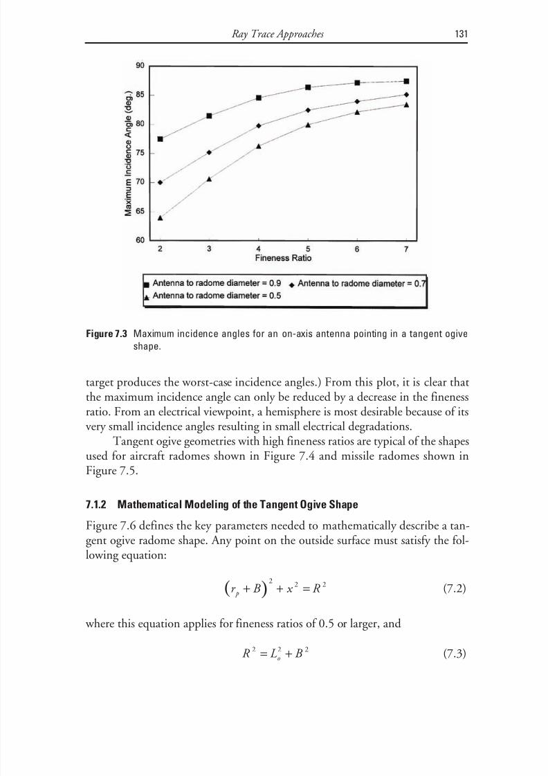
8/20/2019 Analysis of Radome-Enclosed Antennas
http://slidepdf.com/reader/full/analysis-of-radome-enclosed-antennas 152/319
target produces the worst-case incidence angles.) From this plot, it is clear thatthe maximum incidence angle can only be reduced by a decrease in the finenessratio. From an electrical viewpoint, a hemisphere is most desirable because of itsvery small incidence angles resulting in small electrical degradations.
Tangent ogive geometries with high fineness ratios are typical of the shapesused for aircraft radomes shown in Figure 7.4 and missile radomes shown inFigure 7.5.
7.1.2 Mathematical Modeling of the Tangent Ogive Shape
Figure 7.6 defines the key parameters needed to mathematically describe a tan-gent ogive radome shape. Any point on the outside surface must satisfy the fol-lowing equation:
( )r B x R p + + =2 2 2 (7.2)
where this equation applies for fineness ratios of 0.5 or larger, and
R L B o 2 2 2= + (7.3)
Ray Trace Approaches 131
Figure 7.3 Maximum incidence angles for an on-axis antenna pointing in a tangent ogive
shape.
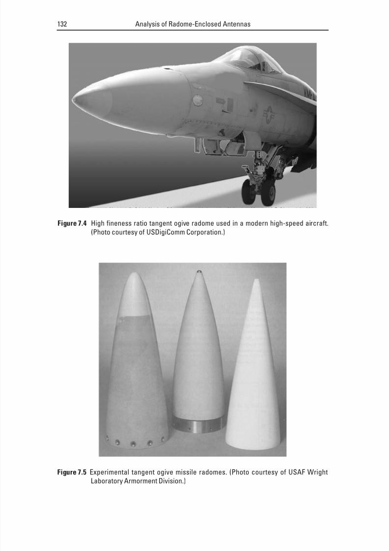
8/20/2019 Analysis of Radome-Enclosed Antennas
http://slidepdf.com/reader/full/analysis-of-radome-enclosed-antennas 153/319
132 Analysis of Radome-Enclosed Antennas
Figure 7.4 High fineness ratio tangent ogive radome used in a modern high-speed aircraft.
(Photo courtesy of USDigiComm Corporation.)
Figure 7.5 Experimental tangent ogive missile radomes. (Photo courtesy of USAF Wright
Laboratory Armorment Division.)

8/20/2019 Analysis of Radome-Enclosed Antennas
http://slidepdf.com/reader/full/analysis-of-radome-enclosed-antennas 154/319
D R B o
2
= − (7.4)
By the simultaneous solution of these two equations, we obtain expres-sions for the two unknowns in terms of the radome length and diameter,respectively:
B L D
D o o
o
= −4
4
2 2
(7.5)
R L D
D o o
o
= −4
4
2 2
(7.6)
Since in the development here in the x -axis corresponds to the radomeaxis, the radome shape is a surface of revolution formed by revolving a tangentogive shape about the x -axis. The cross sections through this three-dimensionalshape are circular in the y -z plane with the radome radius given by the formula:
r z y p p p = +2 2 (7.7)
Ray Trace Approaches 133
Figure 7.6 Mathematical description of a tangent ogive radome geometry.

8/20/2019 Analysis of Radome-Enclosed Antennas
http://slidepdf.com/reader/full/analysis-of-radome-enclosed-antennas 155/319
7.1.3 Determining the Intercept Point of a Ray with the Tangent Ogive Wall
All ray trace analysis methods require the determination of the point of interceptof a ray and the radome surface [6]. Some radome shapes such as the cone lendthemselves to an exact solution of the intercept point. Other shapes such as theVon Karman do not [7]. This section discusses three methods of determining the intercept point.
7.1.3.1 Method 1
Huddleston and Baluis [8] introduced a method for finding the intercept pointthat can apply to the tangent ogive radome geometry. Using this method, the
outer radome shape can be represented by samples spaced equally along theradome axis. Any two sample points are sufficient to define a cone with the ver-tex beyond the tip and opening toward the radome base. Between the samplepoints, the intersection of an incident ray and the cone approximates the pointof intersection with the actual surface. The intersection point is then refined,using additional sample points and a perturbational technique.
7.1.3.2 Method 2
Joy and Ball [9] also reported the development of a ray intercept technique.They specified the radome surface as cylindrical radius values for constant sta-tion (z -position) values. This method of radome shape specification is typical of radome shape data available to the radome analyst.
The technique is an interactive algorithm that locally approximates theradome surface as a cone that is tangent to the radome surface at the point of theray intercept point. Using the interactive algorithm, the analyst can iteratively vary the fineness ratio and the location of the cone axis so that the intersectionpoint of the ray and the cone equals the intersection point of the ray and theradome surface. Convergence is always possible for monotonically concaveradome shapes.
7.1.3.3 Method 3
This method of determining the intercept point is, like Method 2, an iterativemethod. However, it is more general than the two previously discussed methodsand is particularly well suited to computer use. It is very practical particularly
because of the greatly increased speed of PCs that has occurred since the firstedition of this book. This technique uses a generalized ray tracing method fortangent ogive shapes that are treated as surfaces of revolution formed by revolv-ing a single-valued plane curve about the radome axis.
Referring to Figure 7.7, the problem starts with definition of a vector orig-inating at a point P (x o , y o , z o ) within the radome and having a propagation
134 Analysis of Radome-Enclosed Antennas

8/20/2019 Analysis of Radome-Enclosed Antennas
http://slidepdf.com/reader/full/analysis-of-radome-enclosed-antennas 156/319

8/20/2019 Analysis of Radome-Enclosed Antennas
http://slidepdf.com/reader/full/analysis-of-radome-enclosed-antennas 157/319

8/20/2019 Analysis of Radome-Enclosed Antennas
http://slidepdf.com/reader/full/analysis-of-radome-enclosed-antennas 158/319
Ray Trace Approaches 137
Figure 7.9 Illustration of propagation vector when it is outside the radome.
Figure 7.10 Computer software flow diagram for the program OGIVE rootfinder algorithm.

8/20/2019 Analysis of Radome-Enclosed Antennas
http://slidepdf.com/reader/full/analysis-of-radome-enclosed-antennas 159/319
methods. The approach first increments coarse, then medium, and then fineincrements in the C i values until detecting the zero crossing of ERF to withinthe finest increment of C i . In the flow diagram shown, these increments corre-
spond to 1.0 inch, 0.1 inch, and 0.01 inch, respectively. Note that the first itera-tion cycle (i = 1 to 100) assumes that the maximum radome size is 100 inches. If your radome is larger, adjust this parameter accordingly.
Appendix 7A is a sample computer program listing that shows this partic-ular rootfinder. This program incorporates a subroutine that models the tangentogive radome shape discussed earlier in this chapter. The development works fortangent ogive radomes having a hemispherical shape, L o /D o = 0.5, or higher fine-ness ratios. Typically, this program takes from 10 to 25 cycles to find the inter-cept point to within an accuracy of 0.01 inch.
7.1.4 Computation of Surface Normal Vector at the Intercept Point
For any point P (x o , y o , z o ) on the tangent ogive contour, the slope of the curve isfound from:
m x
r B
x
y z B
o
p
o
o o
= −
+
= −
+ +2 2
(7.14)
Referring back to Figure 7.6, the slope of the normal vector is then foundfrom
( )tan ψ = −
= +
= + +1
2 2
m
r B
x
y z B
x o
o
o o
o
(7.15)
From this, the x -component of the surface normal vector is:
n r B
x y z B
x
x
o
o
o o
o
= =
+ +
=
+ + +
cos ψ 1
1
1
1
22 2
2(7.16)
The y- and z -components of the normal vector depicted in Figure 7.11 are
138 Analysis of Radome-Enclosed Antennas

8/20/2019 Analysis of Radome-Enclosed Antennas
http://slidepdf.com/reader/full/analysis-of-radome-enclosed-antennas 160/319
n
r B
x
r B x
y
r
y
o
o
o
o
o
o
= =
+
+ +
sin sin ψ φ
1
2(7.17)
n
y z B
x
y z B x
y
z y
o o
o
o o
o
o
o
=
+ +
+ + +
+
2 2
2 22 2
1 y o
2(7.18)
n
r B
x
r B
x
z
r z
o
o
o
o
o
o
= =
+
+
+
sin cos ψ φ
1
2(7.19)
Ray Trace Approaches 139
Figure 7.11 Components of the surface normal vector in the y -z plane.

8/20/2019 Analysis of Radome-Enclosed Antennas
http://slidepdf.com/reader/full/analysis-of-radome-enclosed-antennas 161/319
n
y z B
x
y z B
x
z
z
z
o o
o
o o
o
o
o
=
+ +
+ + +
+
2 2
2 2
2 2
1 y o
2(7.20)
7.1.5 Determining the Ray Angle of Incidence
The transmission of a ray through the radome wall was shown earlier to be a function of the angle of incidence of the propagation vector relative to the sur-
face normal at the intercept point, θ. This can be evaluated from simple vectorrelationships:
cos θ = ⋅ = + +k n k n k n k n x x y y z z (7.21)
( )θ = + + +−cos 1 k n k n k n x x y y z z (7.22)
Since most mathematical PC software does not have an inverse cosinefunction, this can be put into the alternate form
( )θ = − + +−sin 1 21 k n k n k n x x y y z z (7.23)
7.2 Hemispherical Radome Shapes
The ideal radome shape is a spherically shaped radome enclosing a gimbaledantenna. It is ideal for three reasons: (1) the angle of incidence of any ray ema-nating from the enclosed antenna and propagating through the radome wall isrelatively small and generally less than 40° permitting low loss wall designs, (2)because of the symmetry, the angles of incidence do not change with the point-ing angle of the antenna and there are only very small changes in radome trans-mission loss with the pointing angle of the antenna, and (3) there is no boresighterror (BSE) for any antenna pointing angles through the radome wall.
Spherical- or hemispherical-shaped radomes are particularly suited to ter-restrial radar applications depicted in Figure 7.12 or other microwave applica-tions as depicted in Figure 7.13. They are not suited to airborne or missileapplications because of the very large aerodynamic drag. It can be shown thatthe hemisphere is a special case of the tangent ogive shape, but with a finenessratio (ratio of length to base diameter) of 0.5.
140 Analysis of Radome-Enclosed Antennas

8/20/2019 Analysis of Radome-Enclosed Antennas
http://slidepdf.com/reader/full/analysis-of-radome-enclosed-antennas 162/319
Ray Trace Approaches 141
Figure 7.12 Large terrestrial radar antenna in a hemispherical radome. (Photo courtesy of
MFG Galileo.)
Figure 7.13 Small microwave antenna in a hemispherical radome. (Photo courtesy of MFG
Galileo.)

8/20/2019 Analysis of Radome-Enclosed Antennas
http://slidepdf.com/reader/full/analysis-of-radome-enclosed-antennas 163/319
7.3 Other Radome Shapes Having Axial Symmetry
7.3.1 Mathematical Modeling of the Radome Shape
This section discusses radomes whose shape is rotationally symmetric but noteasily described mathematically in a closed form solution such as the tangentogive radome shape. If the radius (r p ) is known as a function of distance from theradome base (x p ), then the data can be fitted to a polynomial equation using theleast squares method. For instance, consider modeling the shape with a fifth-order polynomial:
r A A x A x A x A x A x p o p p p p p = + + + + +1 22
33
4
4
5
5 (7.24)
The coefficients of this expression can be evaluated with a polynomialregression such as that shown in Appendix 7B by manually inputting as many data sets of r p and x p as practical: the computer program computes the values of each of the coefficients. The software code solves this system of equations andcomputes the unknown coefficients. The next section describes the procedurefor using this program.
7.3.2 POLY Polynomial Regression Subroutine
This software listing in Appendix 7B is in POWERBASIC [11]. Before running the program, have a table with the {z p , r p } data sets that describe the radome. Theprogram will do the least squares fit regression analysis to insure the approxima-tion is as close as possible over the entire range of the data. The number of data points that should be entered to get a good approximation is something of a trial-and-error process. Too few points may be insufficient for an accurateapproximation, whereas too many are tedious to enter and will not significantly
improve the data.To run the program, perform the following steps:
1. Enter first the z p , and next the r p values for the first data pair, as you areprompted. When entering values, you may edit them with the back-space key before you press [Return]. You can abort execution at any point by pressing [Ctrl-Break].
2. Enter the rest of the data sets as the program prompts you.
3. Type “E” to exit the data entry screen after you have entered the finalpair.
4. Wait for the program to run the regression analysis, ending by the dis-play of the coefficients, A 0 through A 5, that provide the best leastsquares approximation to your data.
142 Analysis of Radome-Enclosed Antennas
8/20/2019 Analysis of Radome-Enclosed Antennas
http://slidepdf.com/reader/full/analysis-of-radome-enclosed-antennas 164/319
5. Enter a value of z p when prompted, to test this approximation by allowing you to see what value of r p results.
6. Enter Q (for quit). The program will ask if you want to try the regres-
sion analysis again with a different set of input data. Enter Y (yes) orN (no) as required.
7.3.3 Determining Intercept Point and Surface Normal Vectors
Once the coefficients are evaluated, we can find a ray intercept point and surfacenormal vector for a tangent ogive radome via the previously developed Method3 of Section 7.2. Specifically, the error function ERF needed to be used to findthe intercept point must be expressed in terms of these polynomial coefficients
and is given by the formula:
( )ERF r r A A x A x A x A x A x
y z
p i i i i i i
i i
= − = + + + + +
− +
0 1 22
33
4
4
5
5
2 2
(7.25)
To find the intercept of a propagation vector emanating from the pointP (x o , y o , z o ) and the radome wall, we need to vary the parameter C i in (7.10),(7.12), and (7.13) adaptively until the error function ERF is zero. Once theintercept point is determined, the slope of the radome shape at the interceptpoint is found from
m A A x A x A x A x i i i i = + + + +1 2 32
4
3
5
42 3 4 5 (7.26)
The slope of the unit normal vector is
tan ψ = −
= −
+ + + +1 1
2 3 4 51 2 32
4
3
5
4m A A x A x A x A x i i i i
(7.27)
We can resolve the three components of the normal vector following (7.16) through (7.19) and can compute the angle of incidence of an arbitrary ray and its intercept at the radome wall via (7.21).
Appendix 7C is a sample computer program listing that applies a simple
rootfinder to the arbitrary shape as discussed in this section. Typically, this pro-gram takes from 10 to 25 cycles to find the intercept point to within an accuracy of 0.01 inch.
Ray Trace Approaches 143

8/20/2019 Analysis of Radome-Enclosed Antennas
http://slidepdf.com/reader/full/analysis-of-radome-enclosed-antennas 165/319
7.4 Wave Decomposition at the Intercept Point
The flat-plate voltage transmission coefficients of the radome wall must weightthe incident electric field associated with each ray. The problem geometry isillustrated in Figure 7.14, which shows an arbitrarily polarized wave E i incidenton a dielectric wall at angle θ with respect to the unit surface normal at the inter-cept point. The assumptions are that: (1) the wave is a plane wave consistent
with ray tracing, and (2) the wall will be treated as locally plane at the ray inter-cept point.
To apply transmission coefficients to the wave as it propagates through the wall, we must first resolve the arbitrarily polarized incident wave into compo-nents parallel and perpendicular to the plane of incidence.
Decomposition of the incident electric field into two orthogonal vectorcomponents follows from vector mathematics. First, it is necessary to determineunit vectors perpendicular and parallel to the plane formed by the surface nor-mal vector, n , and the direction of propagation vector, k . The perpendicularvector is given by [12, 13]:
( )
( ) ( )( )
D n k
n k n k x n k n k y n k n k z
n k n k n
y z z y z x x z x y y x
y z z y
= ×
= − + − + −
− +2 ( ) ( )z x x z z y y x k n k n k n k − + −2 2
(7.28)
or
144 Analysis of Radome-Enclosed Antennas
Figure 7.14 Decomposition of an incident wave into parallel and perpendicular components.
8/20/2019 Analysis of Radome-Enclosed Antennas
http://slidepdf.com/reader/full/analysis-of-radome-enclosed-antennas 166/319
D d x d y d z x y z = + + (7.29)
and the parallel vector by:
( ) ( ) ( )( )
G D k
d k d k x d k d k y d k d k z
d k d k d
y z z y z x x z x y y x
y z z y
= ×
= − + − + −
− +2 ( ) ( )z x x z x y y x k d k d k d k − + −2 2
(7.30)
or
G g x g y g z x y z = + + (7.31)
We can also represent any transverse electromagnetic wave as two orthogo-nally polarized waves. Let Ei represent the electric field of a wave incident on the
wall, as in Figure 7.14. Since this vector field is a complex function, we will rep-resent the incident field in a phasor notation similar to that used by variousauthors [14–16].
E E x E y E z i i x
i x y
i y z
i z ∠ = ∠ + ∠ + ∠ γ γ γ γ (7.32)
wherein γx , γ y , γz represent the relative phase angle of each of the three compo-nents of Ei.
For an example, assume that we are sufficiently into the far field of thesource antenna where the phase is relatively uniform. Note also that right-handcircular polarization occurs if the y -component has a net 90° phase shift com-
pared with the horizontal component. A left-hand circular wave y -componenthas a net −90° phase shift compared with the horizontal component. The Insti-tute of Electrical and Electronic Engineers (IEEE) standards define the sense tobe right-hand if the electric vector rotates in a clockwise direction for anobserver looking in the direction of propagation. The sense is right-hand circu-lar if the electric vector rotates in the opposite direction.
Also as illustrated in Figure 7.14, the incident vector field is resolved intoscalar components perpendicular and parallel to the plane of incidence by vectordot products of Ei, respectively. The result obtained is:
E E d E d E d i i x i
x x y i
y y z i
z z ⊥ ⊥∠ = ∠ + ∠ + ∠ γ γ γ γ (7.33)
E E g E g E g i i x i
x x y i
y i
y z i
z z ∠ = ∠ + ∠ + ∠ γ γ γ γ (7.34)
Ray Trace Approaches 145

8/20/2019 Analysis of Radome-Enclosed Antennas
http://slidepdf.com/reader/full/analysis-of-radome-enclosed-antennas 167/319
The transmitted field is expressed as the product of the incident field andthe complex voltage transmission coefficients for each of the two orthogonal lin-ear polarizations. Therefore, the magnitude and phase of each of the two com-
ponents of the transmitted field are:
( )E E T IPD t t i w
i ⊥ ⊥ ⊥ ⊥ ⊥ ⊥∠ = ∠ + γ γ (7.35)
( )E E T IPD t t i
w
i ∠ = ∠ +⊥ γ γ (7.36)
where T w ⊥, T w
are the voltage transmission coefficient for the perpendicularand parallel wave components, respectively (dimensionless), and IPD
⊥ and
IPD are the insertion phase delays for the perpendicular and parallel wave com-ponents, respectively (radians).
We can now recombine vector components to obtain the transmitted vec-tor field.
( )
( )
E E d E g x
E d E g y
E d
t t t
x t t
x t
t y
t t y
t
t z
∠ = ∠ + ∠ +
∠ + ∠ +
∠
⊥ ⊥
⊥ ⊥
⊥
γ γ γ
γ γ
( ) γ ⊥ + ∠t t z
t E g z
(7.37)
Subroutine COMPOSE (Appendix 7D) shows a sample computer pro-gram for an electromagnetic wave decomposition and recomposition using thisapproach. The program breaks the wave into parallel and perpendicular compo-nents, applies the complex, plane-wave, wall transmission coefficients, andreturns a complex result for the transmitted electric field.
References
[1] Groutage, F. D., Radome Development for a Broadband RF Missile Sensor , Research ReportNELC-TR-2023, San Diego, CA, Naval Electronics Laboratory Center, January 1977.
[2] Chin, S. S., Missile Configuration Design , New York: McGraw-Hill, 1981.
[3] Weckesser, L. B., “Thermal-Mechanical Design Principles,” Ch. 3 in Radome Engineering
Handbook , J. D. Walton, Jr., (ed.), New York: Marcel Dekker, 1970.
[4] Yost, D. J., L. B. Weckesser, and R. C. Mallalieu, Technology Survey of Radomes for Anti-Air Homing Missiles , Applied Physics Laboratory Report FS 80-022, Laurel, MD, John Hopkins University, March 1980.
146 Analysis of Radome-Enclosed Antennas

8/20/2019 Analysis of Radome-Enclosed Antennas
http://slidepdf.com/reader/full/analysis-of-radome-enclosed-antennas 168/319
[5] Crowe, B., Air Launched Tactical Missile Radome Study , Newport Beach, CA, Flight Sys-tems, Inc., January 1977.
[6] Joy, E. B., and G. K. Huddleston, Radome Effects on the Performance of Ground Mapping Radar , Final Technical Report on Research Contract DAAH01-72-C-0598, Atlanta, GA,Georgia Institute of Technology, March 1973.
[7] Walton, J. D., (ed.), Radome Engineering Handbook , New York: Marcel Decker, 1970.
[8] Huddleston, G. K., and A. R. Balius, “A Generalized Ray Tracing Method for Single Val-ued Radome Surfaces of Revolution,” Proceedings of the 15th International Symposium on Electromagnetic Windows , Georgia Institute of Technology, Atlanta, GA, June 1980.
[9] Joy, E. B., and D. E. Ball, “Fast Ray Tracing Algorithm for Arbitrary Monotonically Con-cave Three-Dimensional Radome Shapes,” Proceedings of the 17th International Symposium on Electromagnetic Windows , Georgia Institute of Technology, Atlanta, GA, July 1984.
[10] Adams, L. J., and P. A. White, Analytic Geometry and Calculus , London, England: OxfordUniversity Press, 1968, p. 542.
[11] www.powerbasic.com.
[12] Seber, G. A. F., Linear Regression Analysis , New York: John Wiley & Sons, 1977.
[13] Johnson, L. W., and R. D. Riess, Introduction to Linear Algebra , Reading, MA: Addi-son-Wesley Publishing Company, 1981.
[14] Kreyszig, E., Advanced Engineering Mathematics, New York: John Wiley & Sons, 1962.
[15] Pipes, L. A., and L. R. Harvell, Applied Mathematics for Engineers and Physicists , 3rd ed.,New York: McGraw-Hill, 1970.
[16] Hollis, J. S., T. J. Lyon, and L. Clayton, Jr., Microwave Antenna Measurements , 2nd ed., Atlanta, GA: Scientific Atlanta, Inc., 1970.
Appendix 7A: Program OGIVE Software Listing
#COMPILE EXEFUNCTION PBMAIN
‘ PROGRAM OGIVE TO COMPUTE INTERCEPT POINT ON TANGENT OGIVE RADOME
GLOBAL L0, D0, R, B, X0, Y0, Z0, AZ, EL, DRAD, PI, AZD, ELD, Ci AS
SINGLE
GLOBAL Kx, Ky, Kz, ERF, rp, ri, Xi, Yi, Zi, Xp, Yp, Zp, ACCUM AS SINGLE
GLOBAL Nx, Ny, Nz, THETA AS SINGLE
GLOBAL COUNT AS INTEGER
PI=3.14159265
DRAD = PI/180
‘ L0 = length of radome (cm)
‘ D0 = base diameter of radome (cm)
‘ X0, Y0, Z0 = coordinates of initial point on antenna aperture
‘ Kx, Ky, Kz = propagation vector
‘ Xi, Yi, Zi = coordinates of tip of ray (cm)
‘ Xp, Yp, Zp = intercept point on radome when rp = ri
‘ ri = radius at tip of ray for value Xi (cm)
‘ rp = radius at actual radome surface for value Xi (cm)
‘ ERF = error function - rp - ri = distance from tip of ray to radome
Ray Trace Approaches 147

8/20/2019 Analysis of Radome-Enclosed Antennas
http://slidepdf.com/reader/full/analysis-of-radome-enclosed-antennas 169/319
‘ AZD, ELD = angular directions of propagation vector (degrees)
‘ AZ, EL = angular directions of propagation vector
‘ (radians)
‘ Note: AZ=0 EL=0 corresponds to Kx=1, Ky=0, Kz=0
‘ Nx, Ny, Nz are the components of the surface normal vector at the
‘ intercept point (cm)‘ THETA is the angle of incidence between the propagation vector and
‘ the normal vector at the incidence point (radians)
‘ To demonstrate program assume:
X0=0: Y0=0: Z0=0
L0 = 100
D0 = 50
R=(4*L0^2+D0^2)/(4*D0)
B=(4*L0^2-D0^2)/(4*D0)
ELD=0
FOR AZD=0 TO 90 STEP 30
AZ=AZD*DRADEL=ELD*DRAD
Kx=COS(AZ)*COS(EL)
KY=SIN(AZ)
KZ=COS(AZ)*SIN(EL)
FOR COUNT=0 TO 100.5
Ci=COUNT*1.0
Xi=X0+Ci*Kx
Yi=Y0+Ci*Ky
Zi=Z0+Ci*Kz
ri=SQR(Yi^2+Zi^2)
rp=SQR(R^2-Xi^2) - B
ERF=rp-ri
IF ERF<0 THEN
Ci=Ci-1
GOTO 100
END IF
IF ERF<1 THEN
GOTO 100
END IF
NEXT COUNT
100 ‘CONTINUE
ACCUM = Ci
FOR COUNT=0 TO 10Ci = ACCUM+COUNT*0.1
Xi=X0+Ci*Kx
Yi=Y0+Ci*Ky
Zi=Z0+Ci*Kz
ri=SQR(Yi^2+Zi^2)
rp=SQR(R^2-Xi^2) - B
ERF=rp-ri
IF ERF<0 THEN
Ci=Ci-0.1
GOTO 200
END IF
IF ERF<0.1 THEN
GOTO 200
END IF
NEXT COUNT
200 ‘CONTINUE
ACCUM = Ci
FOR COUNT=0 TO 10
148 Analysis of Radome-Enclosed Antennas

8/20/2019 Analysis of Radome-Enclosed Antennas
http://slidepdf.com/reader/full/analysis-of-radome-enclosed-antennas 170/319
Ci = ACCUM+COUNT*0.01
Xi=X0+Ci*Kx
Yi=Y0+Ci*Ky
Zi=Z0+Ci*Kz
ri=SQR(Yi^2+Zi^2)
rp=SQR(R^2-Xi^2) - BERF=rp-ri
IF ERF<0 THEN
Ci=Ci-0.01
Xi=X0*Ci*Kx
Yi=Y0+Ci*Ky
Zi=Z0+Ci*Kz
GOTO 300
END IF
IF ERF<0.01 THEN
GOTO 300
END IFNEXT COUNT
300 ‘CONTINUE
‘INTERCEPT POINT ON THE RADOME SURFACE IS
Xp=Xi: Yp=Yi: Zp=Zi
Xp=ABS(Xp)
‘NOW TO COMPUTE NORMAL VECTOR AT THE INTERCEPT POINT:
Nx = 1/SQR(1+(rp+B/Xp)^2)
Ny = ((Yp/rp)*((rp+B)/Xp))/SQR(1+((rp+B)/Xp)^2)
Nz = ((Zp/rp)*((rp+B)/Xp))/SQR(1+((rp+B)/Xp)^2)
THETA=ATN((SQR(1-(Nx*Kx+Ny*Ky+Nz*Kz)^2)/(Nx*Kx+Ny*Ky+Nz*Kz)))
PRINT “AZ(deg)=“;AZD;” EL(deg)=“;ELD;” Xp=“;Xp;” Yp=“; Yp;” Zp=“; Zp;
“ THETA(deg)=“; THETA/DRAD
NEXT AZD
PRINT “PUSH THE ENTER KEY TO END PROGRAM”
INPUT hash$
END FUNCTION
Appendix 7B: Program POLY Software Listing
#COMPILE EXE
FUNCTION PBMAIN ()‘ ———————————————————————————————-
‘ Program POLY is a fifth order polynomial regression code
CLS
GLOBAL RP(), XP(), X, Y, A(), MATR(), SM(), RT() AS SINGLE
GLOBAL SM(), RT(), TMP , FTR, TOT AS SINGLE
GLOBAL I, J, K, L, N, KMP, ORDER, ITMP, CNT, PNT, COUNT AS INTEGER
DIM RP(50), XP(50), A(10), MATR(10,10), SM(10), RT(10)
‘ ORDER = ORDER OF REGRESSION
ORDER = 5
‘ N = NUMBER OF DATA POINT PAIRS TO BE ENTERED
‘————————- USER INPUT DATA —————————-
‘ XP = Distance from the radome base (inches)
‘ RP = Radome radius (inches)
PRINT “MIN OF THREE DATA SETS REQUIRED”
INPUT “INPUT NUMBER OF DATA SETS TO BE ENTERED = “; N
Ray Trace Approaches 149

8/20/2019 Analysis of Radome-Enclosed Antennas
http://slidepdf.com/reader/full/analysis-of-radome-enclosed-antennas 171/319
FOR COUNT = 1 TO N
INPUT “XP = “; XP(COUNT)
INPUT “RP = “; RP(COUNT)
NEXT COUNT
PRINTPRINT “WHEN READY TO BEGIN REGRESSION ANALYSIS INPUT ANY KEY”
INPUT HASH$
‘BEGIN POLYNOMIAL REGRESSION ALGORITHM:
FOR I = 1 TO 2 * ORDER
SM(I) = 0
NEXT I
FOR I = 1 TO ORDER + 1
RT(I) = 0
NEXT I
FOR PNT = 1 TO N
FOR I = 1 TO ORDER * 2SM(I) = SM(I) + XP(PNT) ^ I
NEXT I
FOR I = 1 TO ORDER + 1
IF I = 1 THEN RT(I) = RT(I) + RP(PNT)
IF I 1 THEN RT(I) = RT(I) + RP(PNT) * (XP(PNT) ^ (I - 1))
NEXT I
NEXT PNT
MATR(1, 1) = N
FOR I = 1 TO ORDER + 1
MATR(I, ORDER + 2) = RT(I)
FOR J = 1 TO ORDER + 1
IF I + J 2 THEN MATR(I, J) = SM(I + J - 2)
NEXT J
NEXT I
FOR K = 1 TO ORDER
K M P = K + 1
L = K
FOR I = KMP TO ORDER + 1
IF ABS(MATR(I, K)) > ABS(MATR(L, K)) THEN L = I
NEXT I
IF L K THEN
FOR J = K TO ORDER + 2
TMP = MATR(K, J)MATR(K, J) = MATR(L, J)
MATR(L, J) = TMP
NEXT J
END IF
FOR I = KMP TO ORDER + 1
FTR = MATR(I, K) / MATR(K, K)
FOR J = KMP TO ORDER + 2
MATR(I, J) = MATR(I, J) - FTR * MATR(K, J)
NEXT J
NEXT I
NEXT K
A(ORDER + 1) = MATR(ORDER + 1, ORDER + 2) / MATR(ORDER + 1, ORDER + 1)
I = ORDER
DO
I T M P = I + 1
TOT = 0
FOR J = ITMP TO ORDER + 1
TOT = TOT + MATR(I, J) * A(J)
150 Analysis of Radome-Enclosed Antennas

8/20/2019 Analysis of Radome-Enclosed Antennas
http://slidepdf.com/reader/full/analysis-of-radome-enclosed-antennas 172/319
NEXT J
A(I) = (MATR(I, ORDER + 2) - TOT) / MATR(I, I)
I = I - 1
IF I < 1 THEN EXIT DO
LOOP
‘——— DISPLAY COEFFICIENTS ————————————————————
CLS : LOCATE 1, 1
PRINT “COMPUTED COEFFICIENTS”
PRINT “A0 = “; A(1)
PRINT “A1 = “; A(2)
PRINT “A2 = “; A(3)
PRINT “A3 = “; A(4)
PRINT “A4 = “; A(5)
PRINT “A5 = “; A(6)PRINT
PRINT “READY TO TEST CONFORMANCE”
PRINT “PUSH ANY KEY TO BEGIN”
INPUT HASH$
‘———— TEST POLYNOMIAL CONFORMANCE ———————————————-
100 ‘CONTINUE
INPUT “INPUT XP = “; X
Y = A(1) + A(2)*X + A(3)*X^2 +A(4)*X^3 +A(5)*X^4 +A(6)*X^5
PRINT “COMPUTED RP = “; Y
GOTO 100
200 ‘END OF PROGRAM
‘—————————————————————————————————-
END FUNCTION
Appendix 7C: Program ARBITRARY Software Listing
#COMPILE EXEFUNCTION PBMAIN
‘ PROGRAM ARBITRARY TO COMPUTE INTERCEPT POINT ON AN ARBITRARY SHAPED
RADOME
‘ HAVING AXIAL SYMMETRY
GLOBAL X0, Y0, Z0, AZ, EL, DRAD, PI, AZD, ELD, Ci AS SINGLE
GLOBAL Kx, Ky, Kz, ERF, rp, ri, Xi, Yi, Zi, Xp, Yp, Zp, ACCUM AS SINGLE
GLOBAL Nx, Ny, Nz, Nt, THETA, PSI, ALPHA AS SINGLE
‘POLYNOMIAL REGRESSION COEFFICIENTS:
GLOBAL A0, A1, A2, A3, A4, A5 AS SINGLE
GLOBAL COUNT AS INTEGER
PI=3.14159265
DRAD = PI/180
‘ A0 through A5 are polynomial regression coefficients for radome
shape
‘ obtained by use of program POLY
‘ X0, Y0, Z0 = coordinates of initial point on antenna aperture
‘ Kx, Ky, Kz = propagation vector
‘ Xi, Yi, Zi = coordinates of tip of ray (cm)
Ray Trace Approaches 151

8/20/2019 Analysis of Radome-Enclosed Antennas
http://slidepdf.com/reader/full/analysis-of-radome-enclosed-antennas 173/319
‘ Xp, Yp, Zp = intercept point on radome when rp = ri
‘ ri = radius at tip of ray for value Xi (cm)
‘ rp = radius at actual radome surface for value Xi (cm)
‘ ERF = error function - rp - ri = distance from tip of ray to radome
‘ AZD, ELD = angular directions of propagation vector (degrees)
‘ AZ, EL = angular directions of propagation {AU: EDIT OK?} vector(radians)
‘ Note: AZ=0 EL=0 corresponds to Kx=1, Ky=0, Kz=0
‘ Nx, Ny, Nz are the components of the surface normal vector at the
‘ intercept point (cm)
‘ THETA is the angle of incidence between the propagation vector and
the
‘ normal vector at the incidence point (radians)
‘ PSI is the slope of the normal vector
‘ To demonstrate program assume:
X0=0: Y0=0: Z0=0
A0=25.00086A1=-7.41124*10^-4
A2=-2.29406*10^-3
A3=-1.72184*10^-6
A4=+9.11312*10^-9
A5=-1.17584*10^-10
ELD=0
FOR AZD=0 TO 90 STEP 30
AZ=AZD*DRAD
EL=ELD*DRAD
Kx=COS(AZ)*COS(EL)
KY=SIN(AZ)
KZ=COS(AZ)*SIN(EL)
FOR COUNT=0 TO 100
Ci=COUNT*1.0
Xi=X0+Ci*Kx
Yi=Y0+Ci*Ky
Zi=Z0+Ci*Kz
ri=SQR(Yi^2+Zi^2)
rp=A0+A1*Xi+A2*Xi^2+A3*Xi^3+A4*Xi^4+A5*Xi^5
ERF=rp-ri
IF ERF<0 THEN
Ci=Ci-1
GOTO 100END IF
IF ERF<1 THEN
GOTO 100
END IF
NEXT COUNT
100 ‘CONTINUE
ACCUM = Ci
FOR COUNT=0 TO 10
Ci = ACCUM+COUNT*0.1
Xi=X0+Ci*Kx
Yi=Y0+Ci*Ky
Zi=Z0+Ci*Kz
ri=SQR(Yi^2+Zi^2)
rp=A0+A1*Xi+A2*Xi^2+A3*Xi^3+A4*Xi^4+A5*Xi^5
ERF=rp-ri
IF ERF<0 THEN
Ci=Ci-0.1
GOTO 200
152 Analysis of Radome-Enclosed Antennas
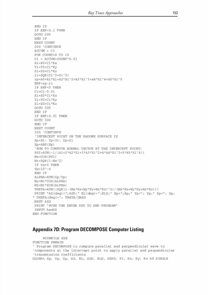
8/20/2019 Analysis of Radome-Enclosed Antennas
http://slidepdf.com/reader/full/analysis-of-radome-enclosed-antennas 174/319
END IF
IF ERF<0.1 THEN
GOTO 200
END IF
NEXT COUNT
200 ‘CONTINUEACCUM = Ci
FOR COUNT=0 TO 10
Ci = ACCUM+COUNT*0.01
Xi=X0+Ci*Kx
Yi=Y0+Ci*Ky
Zi=Z0+Ci*Kz
ri=SQR(Yi^2+Zi^2)
rp=A0+A1*Xi+A2*Xi^2+A3*Xi^3+A4*Xi^4+A5*Xi^5
ERF=rp-ri
IF ERF<0 THEN
Ci=Ci-0.01Xi=X0*Ci*Kx
Yi=Y0+Ci*Ky
Zi=Z0+Ci*Kz
GOTO 300
END IF
IF ERF<0.01 THEN
GOTO 300
END IF
NEXT COUNT
300 ‘CONTINUE
‘INTERCEPT POINT ON THE RADOME SURFACE IS
Xp=Xi: Yp=Yi: Zp=Zi
Xp=ABS(Xp)
‘NOW TO COMPUTE NORMAL VECTOR AT THE INTERCEPT POINT:
PSI=ATN(-1/(A1+2*A2*Xi+3*A3*Xi^2+4*A4*Xi^3+5*A5*Xi^4))
Nx=COS(PSI)
Nt=SQR(1-Nx^2)
IF Yp=0 THEN
Yp=10^-6
END IF
ALPHA=ATN(Zp/Yp)
Ny=Nt*COS(ALPHA)
NZ=Nt*SIN(ALPHA)THETA=ATN((SQR(1-(Nx*Kx+Ny*Ky+Nz*Kz)^2)/(Nx*Kx+Ny*Ky+Nz*Kz)))
PRINT “AZ(deg)=“;AZD;” EL(deg)=“;ELD;” Xp=“;Xp;” Yp=“; Yp;” Zp=“; Zp;
“ THETA(deg)=“; THETA/DRAD
NEXT AZD
PRINT “PUSH THE ENTER KEY TO END PROGRAM”
INPUT hash$
END FUNCTION
Appendix 7D: Program DECOMPOSE Computer Listing
#COMPILE EXE
FUNCTION PBMAIN
‘ Program DECOMPOSE to compute parallel and perpendicular wave to
‘components at the intercept point to apply parallel and perpendicular
‘transmission coefficients
GLOBAL Xp, Yp, Zp, AZ, EL, AZD, ELD, DRAD, PI, Kx, Ky, Kz AS SINGLE
Ray Trace Approaches 153

8/20/2019 Analysis of Radome-Enclosed Antennas
http://slidepdf.com/reader/full/analysis-of-radome-enclosed-antennas 175/319
GLOBAL Nx, Ny, Nz, Dt, Gt, Dy, Dz, Gx, Gy, Gz, Tpara, Tperp, Dx AS
SINGLE
GLOBAL Eix, Eiy, Eiz, Etx, Ety, Etz, THETA, Ei, Et, Eipara, Eiperp AS
SINGLE
GLOBAL Etpara, Etperp, T, TdB, Nt, Kt, Eit, Ett AS SINGLE
PI=3.14159265DRAD = PI/180
‘Xp, Yp, Zp = coordinate of intercept point on radome surface
‘AZD, ELD = angular directions of propagation vector (degrees)
‘AZ, EL = angular directions of propagation {AU: EDIT OK?} vector
(radians)
‘Note: AZ=0, EL=0 cprres[pmds tp Lx=1, Ky=0, Kz=0
‘Nx, Ny, Nz = the components of the surface normal vector at the inter-
cept point (cm)
‘THETA is the angle of incidence between the propagation vector and
the normal
‘vector at the incidence point (radians)‘ —————————————————————————————————————————-
‘To illustrate the procedure, assume that:
AZD=30: ELD=30
AZ = AZD*DRAD
EL = ELD*DRAD
‘Rotate aperture E vector through AZ and EL angles:
‘(Assume vertical polarization for this sample problem)
Eix = -SIN(EL)*COS(AZ)
Eiy = -SIN(EL)*SIN(AZ)
Eiz = +COS(EL)
Eit=SQR(Eix^2+Eiy^2+Eiz^2)
PRINT “PRINT Eit TO CONFIRM THAT Eit IS A UNIT VECTOR:”
PRINT Eit
‘If horizontal polarization these expressions would be:
‘Eix = -SIN(AZ)
‘Eiy = +COS(AZ)
‘Eiz = 0
Xp=26.325: Yp=17.55: Zp=15.1974
Nx=0.05573592: Ny=0.9592745: Nz=0.2769187
Kx=0.75: Ky=0.5: Kz=0.4330127
‘Parallel and perpendicular polarization wall voltage transmission
coefficients:Tpara = 0.8
Tperp = 0.9
‘Note: for this sample problem we will assume Tpara and Tperp totally
real
‘ —————————————————————————————————————————
‘Starting with these values {AU: EDIT OK?}, compute the components of
vector D
‘Note: D is perpendicular to the plane formed by the vectors K and N
Dx=(Ny*Kz-Nz*Ky)/SQR((Ny*Kz-Nz*Ky)^2+(Nz*Kx-Nx*Kz)^2+(Nx*Ky-Ny*Kx)^2)
Dy=(Nx*Kz-Nz*Kx)/SQR((Ny*Kz-Nz*Ky)^2+(Nz*Kx-Nx*Kz)^2+(Nx*Ky-Ny*Kx)^2)
Dz=(Nx*Ky-Ny*Kx)/SQR((Ny*Kz-Nz*Ky)^2+(Nz*Kx-Nx*Kz)^2+(Nx*Ky-Ny*Kx)^2)
PRINT “PRINT D TO CONFIRM THAT D IS A UNIT VECTOR:”
Dt=SQR(Dx^2+Dy^2+Dz^2)
PRINT Dt
‘Note: G is in the plane formed by the vectors K and N
Gx=(Dy*Kz-Dz*Ky)/SQR((Dy*Kz-Dz*Ky)^2+(Dz*Kx-Dx*Kz)^2+(Dx*Ky-Dy*Kx)^2)
Gy=(Dx*Kz-Dz*Kx)/SQR((Dy*Kz-Dz*Ky)^2+(Dz*Kx-Dx*Kz)^2+(Dx*Ky-Dy*Kx)^2)
154 Analysis of Radome-Enclosed Antennas

8/20/2019 Analysis of Radome-Enclosed Antennas
http://slidepdf.com/reader/full/analysis-of-radome-enclosed-antennas 176/319
Gz=(Dx*Ky-Dy*Kx)/SQR((Dy*Kz-Dz*Ky)^2+(Dz*Kx-Dx*Kz)^2+(Dx*Ky-Dy*Kx)^2)
PRINT “PRINT G TO CONFIRM THAT G IS A UNIT VECTOR:”
Gt=SQR(Gx^2+Gy^2+Gz^2)
PRINT Gt
PRINT‘The perpendicular component of Ei is
Eiperp = Eix*Dx + Eiy*Dy + Eiz*Dz
‘From which
Etperp = Eiperp*Tperp
‘The parallel component of Ei is
Eipara = Eix*Gx + Eiy*Gy +Eiz*Gz
‘From which
Etpara = Eipara*Tpara
Ei = SQR(Eipara^2 + Eiperp^2)
Et = SQR(Etpara^2 + Etperp^2)
T = Et/EiTdB = 20*LOG10(T)
PRINT “TRANSMISSION LOSS FACTOR = “; T; “ TRANSMISSION LOSS (dB)= “;
TdB
INPUT hash$
END FUNCTION
Ray Trace Approaches 155

8/20/2019 Analysis of Radome-Enclosed Antennas
http://slidepdf.com/reader/full/analysis-of-radome-enclosed-antennas 177/319

8/20/2019 Analysis of Radome-Enclosed Antennas
http://slidepdf.com/reader/full/analysis-of-radome-enclosed-antennas 178/319
8Radome-Enclosed Guidance Antennas
This chapter introduces computerized techniques to analyze radome-enclosedguidance antenna systems. A guidance antenna functions to detect the targetlocation, and the currently most commonly used ones are monopulse antennas.Typically, radomes associated with these antennas are aerodynamically stream-lined and have a high fineness ratio (up to 3 or greater). For specific applica-tions, the radome materials must be chosen to simultaneously satisfy structural,
environmental, and electrical requirements. The computerized analysis tech-niques in this chapter can determine the effect of the radome on the perfor-mance of the enclosed antenna and its electronics processing function.
A monopulse antenna is generally forward-mounted in an aircraft or mis-sile, as depicted in Figure 8.1. The term monopulse refers to a signal-processing technique in which only a single radar return pulse is needed to resolve a target’slocation in both the elevation and azimuth planes of the antenna. Monopulsesystems are typically active radar, but in certain applications they may be passive
receptors as with semi-active guidance systems. In this book, the term “seeker” isused synonymously with monopulse electronics systems.Ideally, a radome protects the monopulse antenna from the adverse flight
environment while having an insignificant effect on the electrical performanceof the enclosed antenna. However, in practice a radome always changes the elec-trical performance of the monopulse antenna because of the following factors:(1) dissipative losses within the dielectric material, (2) electrical phase shiftsintroduced by the presence of the radome, and (3) internal reflections. Thesechanges produced by the radome manifest themselves as follows:
157

8/20/2019 Analysis of Radome-Enclosed Antennas
http://slidepdf.com/reader/full/analysis-of-radome-enclosed-antennas 179/319
• Decreased antenna gain;
• Increased antenna beamwidth and sidelobe levels;
• Decreased monopulse null depth;
• Introduction of a boresight error and boresight error slope, which are
functions of the antenna scan angle [1, 2].
In this chapter, antenna pattern calculations are made in steps, which mustbe performed in sequence as follows:
158 Analysis of Radome-Enclosed Antennas
Figure 8.1 Radome-enclosed monopulse antenna used for missile guidance. (Photo cour- tesy of Hughes Aircraft Missile Systems Division.)

8/20/2019 Analysis of Radome-Enclosed Antennas
http://slidepdf.com/reader/full/analysis-of-radome-enclosed-antennas 180/319
1. Transpose all aperture points to radome coordinates.
2. Transform all ray vectors from aperture sample points in the patternlook direction.
3. Compute the antenna pattern space phase terms.4. Determine all ray intercept points on the radome surface.
5. Determine angles of incidence of these rays with respect to the radomesurface normal at each intercept point.
6. Compute the complex voltage transmission coefficients for each ray.
7. Perform an antenna aperture integration.
Section 8.1 provides a definition of BSE and BSES. Section 8.2 discussesantenna patterns and monopulse error voltages for a monopulse antenna with-out a radome, whereas Section 8.3 deals with the same antenna but when it isenclosed within a dielectric radome. Finally, Section 8.4 covers radome model-ing considerations, including rain erosion, aerothermal heating, and radomeeffects on a conscan antenna.
8.1 Definitions of Boresight Error (BSE) and Boresight Error Slope
(BSES)
When used in missiles, the seeker antenna is a key part of the guidance system, which also includes the radome, receiver, autopilot, and airframe. The seeker hasseveral functions:
• To measure the line of sight (or line-of-sight angular rates);
• To measure the range to target and the closing velocity;
• To provide steering commands to the missile autopilot and control sur-faces [3–7].
Figure 8.2 shows a representative closed-loop servo control system, in which the signals received by the missile-mounted seeker antenna are used toguide the missile to the target. This guidance is accomplished in the tracking loop, which is driven by the monopulse elevation and azimuth plane guidanceerror voltages.
The seeker initially finds the target in angle space through the seekerantenna’s beamwidth. The antenna beam is steered by one of the following methods:
• A gimbal that mechanically moves the entire antenna structure;
Radome-Enclosed Guidance Antennas 159

8/20/2019 Analysis of Radome-Enclosed Antennas
http://slidepdf.com/reader/full/analysis-of-radome-enclosed-antennas 181/319
160 Analysis of Radome-Enclosed Antennas
F i g u r e
8 . 2
R e p r e s
e n t a t i v e g u i d a n c e s y s t e m
b l o
c k d i a g r a m .
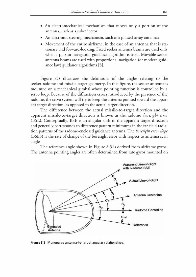
8/20/2019 Analysis of Radome-Enclosed Antennas
http://slidepdf.com/reader/full/analysis-of-radome-enclosed-antennas 182/319
• An electromechanical mechanism that moves only a portion of theantenna, such as a subreflector;
• An electronic steering mechanism, such as a phased-array antenna;
• Movement of the entire airframe, in the case of an antenna that is sta-tionary and forward-looking. Fixed seeker antenna beams are used only
when a pursuit navigation guidance algorithm is used. Movable seekerantenna beams are used with proportional navigation (or modern guid-ance law) guidance algorithms [8].
Figure 8.3 illustrates the definitions of the angles relating to theseeker-radome and missile-target geometry. In this figure, the seeker antenna is
mounted on a mechanical gimbal whose pointing function is controlled by a servo loop. Because of the diffraction errors introduced by the presence of theradome, the servo system will try to keep the antenna pointed toward the appar-ent target direction, as opposed to the actual target direction.
The difference between the actual missile-to-target direction and theapparent missile-to-target direction is known as the radome boresight error (BSE). Conceptually, BSE is an angular shift in the apparent target directionand generally corresponds to difference pattern minimums in the far-field radia-
tion patterns of the radome-enclosed guidance antenna. The boresight error slope (BSES) is the rate of change of the boresight error with respect to antenna scanangle.
The reference angle shown in Figure 8.3 is derived from airframe gyros.The antenna pointing angles are often determined from rate gyros mounted on
Radome-Enclosed Guidance Antennas 161
Figure 8.3 Monopulse antenna-to-target angular relationships.

8/20/2019 Analysis of Radome-Enclosed Antennas
http://slidepdf.com/reader/full/analysis-of-radome-enclosed-antennas 183/319
the antenna gimbal. The monopulse error voltages are fed back to the autopilot.In response to the autopilot commands, the missile changes attitude, whichcauses the antenna to receive through an ever-changing portion of the radome.
As a consequence, the response characteristics of the airframe and autopilot gen-erate a pseudo-noise influence due to these radome-induced errors [9].
8.2 Calculation of Antenna Patterns and Monopulse Error Voltagesfor an Antenna Without a Radome
The physical aperture of a monopulse antenna is usually divided into four quad-rants. Each of these is fed by a microwave network that resolves the signals
received by each of the four quadrants into a sum channel and into elevation andazimuth plane difference channels, as illustrated in Figure 8.4. A monopulseradar receiver processes these sum and difference channel signals as complex voltages, which are resolved into in-phase (I) and out-of-phase or phase quadra-ture (Q) voltages prior to processing by the signal processor.
The sum channel antenna pattern corresponds to a single on-boresightantenna beam, with the half-power beamwidth dictated by both the antenna aperture size in wavelengths and the aperture illumination function. The eleva-
tion channel antenna pattern has a boresight null only in the elevation plane, while the azimuth channel antenna pattern has a boresight null only in the azi-muth plane. The effective sum channel beamwidth obtained with a monopulseantenna is the beamwidth of the aperture, and the maximum gain of theaperture is realized.
Early monopulse systems used reflector antennas or lens antennas, withthe monopulse-beam-forming network achieved with a large, complex wave-guide monopulse network. Modern approaches to achieve sum and differencechannel beams have very small beam-forming networks, with little or no aper-ture blockage [10]. These approaches include the waveguide flat-plate array andmicrostrip array configurations. The photograph of Figure 8.5 shows a microstrip, monopulse array antenna, utilizing square patch radiators and hav-ing the feed network on the same substrate as the patch radiators, while Figure8.6 shows a similar circuit topology that uses circular microstrip patch elements.
From the monopulse sum and difference channel voltages, the monopulseazimuth and elevation plane error voltages are derived in the following manner[11]:
V az az =
∆Σ
(8.1)
162 Analysis of Radome-Enclosed Antennas

8/20/2019 Analysis of Radome-Enclosed Antennas
http://slidepdf.com/reader/full/analysis-of-radome-enclosed-antennas 184/319
Radome-Enclosed Guidance Antennas 163
F i g u r e
8 . 4
B l o c k d i a g r a m
o f a t y p i c a l m o n o p u l s
e r a d a r .

8/20/2019 Analysis of Radome-Enclosed Antennas
http://slidepdf.com/reader/full/analysis-of-radome-enclosed-antennas 185/319
V el el =
∆Σ
(8.2)
In a guidance system, these error voltages are used to guide the missiletoward the target.
The array theory provides the tools to compute monopulse antenna pat-terns without the need to apply exact electromagnetic modeling. The following analysis introduces the modeling methodology, and we use the spherical coordi-nate system shown in Figure 8.7 for the calculation of antenna radiationpatterns. In this system:
P (x o , y
o , z
o ) = reference point at the center of the antenna aperture;
P (x , y , z ) = observation point at a distance R from the antenna;P (x
i , y
i , z
i ) = location of the i th sample point on the antenna aperture;
r o = unit vector in the direction from P (x
o , y
o , z
o ) to P (x , y , z );
r i = vector in the direction from P (x
o , y
o , z
o ) to P (x
i , y
i , z
i ).
164 Analysis of Radome-Enclosed Antennas
Figure 8.5 Square microstrip patch array with monopulse comparator on substrate. (Photo
courtesy of Ball Corporation.)

8/20/2019 Analysis of Radome-Enclosed Antennas
http://slidepdf.com/reader/full/analysis-of-radome-enclosed-antennas 186/319
Radome-Enclosed Guidance Antennas 165
Figure 8.6 Circular microstrip patch array. (Photo courtesy of Seavey Engineering.)
Figure 8.7 Coordinate system used in antenna pattern calculations.

8/20/2019 Analysis of Radome-Enclosed Antennas
http://slidepdf.com/reader/full/analysis-of-radome-enclosed-antennas 187/319
The circular antenna aperture lies entirely in the x - y plane and has a radiusgiven by the formula
( ) ( ) ( )r x x y y z z D a i o i o i o o = − + − + − =2 2 2
2 (8.3)
where D a is the antenna diameter.It is customary to obtain current sample points at spacings d x and d y in the
x - and y -planes, respectively. If these spacings are a half-wave or less at the high-est operating frequency, we guarantee that there will be no aliasing into realspace to cause computational errors in the antenna pattern prediction. However,if we are only interested in the main lobe and first sidelobes of the radiation pat-terns, informal testing by the author shows that sample spacings up to a wave-length or more may be acceptable with only small computational errors.
In accordance with Appendix A, we will now assume that the sample pointcurrents are an ensemble of infinitesimal dipoles, each of which is weighted inboth amplitude and phase. Points on the surface of the antenna aperture areuniquely defined via the integers m , n :
r md y nd z i y z = + (8.4)
For distances relatively far from the i th infinitesimal dipole, its radiationpattern has an exponential phase dependence as it expands as a spherical waveand also has a sine-weighted amplitude dependence with a radiation maximumnormal to the dipole. Based on the coordinate system selected, if the dipoles are
y -directed, an appropriate coordinate transformation derives the radiation ele-ment pattern for the i th infinitesimal dipole as:
( )[ ]E e R
i
jkR
i
i
= −−
cos tan tan sin1 θ φ (8.5)
In this equation, k is the free-space wave number at the frequency of inter-est. If the dipoles are x -directed, the radiation element pattern becomes:
( )[ ]E e
R i
jkR
i
i
= −−
cos tan tan cos1 θ φ (8.6)
Under two conditions, the cosine factors in (8.5) and (8.6) will be nearunity over the angle space corresponding to the antenna main beam through thefirst sidelobes. These conditions are:
166 Analysis of Radome-Enclosed Antennas

8/20/2019 Analysis of Radome-Enclosed Antennas
http://slidepdf.com/reader/full/analysis-of-radome-enclosed-antennas 188/319
• The antenna diameter is larger than about five wavelengths.
• We are only interested in the computation of a limited portion of theantenna patterns, such as the main lobe and the first sidelobes.
If the cosine factors are ignored, the impact on computational accuracy will be small when calculating radome transmission loss and first sidelobe degra-dation. However, when estimating far-out sidelobes, the cosine factors areimportant.
Accordingly, based on the MN total current sample points, the antenna array pattern can be determined from the superposition of the infinitesimaldipoles over the entire aperture.
E F e
R T mn
a jkR
mn n
N
m
M mn
=−
==∑∑
11
(8.7)
Here, the coefficients F mn a are the applied current element weight at the
sample points induced by a received signal. In general, these weighting coeffi-cients are complex quantities.
In (8.7), the required computational distance R mn should be sufficiently
into the far field of the antenna. The actual value of R mn depends on the degreeof fine structure desired in the antenna pattern computation. The conventionaldefinition of antenna far field corresponds to the condition wherein
R D
mn a ≥
2 2
λ(8.8)
A one far-field distance is adequate for main lobe and first sidelobe
antenna pattern calculations. However, for antenna aperture distributions thatgive very low sidelobe antenna patterns, it may be necessary to use distances atleast five times greater than (8.8) [12, 13]. If we let the computational distanceapproach infinity, the following approximation holds:
e
R
e
R e
jkR
mn
jkR
o
jkr r mn o
mn o
− −⋅=
(8.9)
Under this condition,
E e
R F e T
jkR
o
mn a jkr r
n
N
m
M o
mn o =−
⋅
==∑∑
11
(8.10)
Radome-Enclosed Guidance Antennas 167

8/20/2019 Analysis of Radome-Enclosed Antennas
http://slidepdf.com/reader/full/analysis-of-radome-enclosed-antennas 189/319
It is customary to drop out the left factor in brackets, [ ], because theantenna pattern is generally described on a sphere of a constant radius, and thisterm just becomes a normalizing constant [14]. This factor will have no impact
on the computation of radome parameters of interest. The antenna pattern thentakes the form:
E F e T mn a jkr r
n
N
m
M mn o = ⋅
==∑∑
11
(8.11)
Using vector mathematics, we note that
( ) ( ) ( )r x x x y y y z z z mn mn o mn o mn o = − + − + − (8.12)
Also, the unit vector in the direction of the observation point is given interms of the directional cosines [15]:
From these last two equations, we can simplify the dot product in (8.10):
r x y z o = + +sin cos sin sin cosθ φ θ φ θ (8.13)
( ) ( )( )r r x x y y
z z mn o mn o mn o
mn o
⋅ = − + − +−
sin cos sin sincos
θ φ θ φθ
(8.14)
If the center of the antenna is at the point x o = y o = z o = 0 and we select allz mn = 0,
( )E F e T mn a jk x y
n
N
m
M mn mn = − +
==∑∑ sin cos sin sinθ φ θ φ
11
(8.15)
then the simplification on the array pattern of the antenna takes the form:
( )E F e T mn a jk k x k y
n
N
m
M x mn y mn = − +
==∑∑
11
(8.16)
where k x and k y are the propagation constants in the x- and y -planes, respectively.The monopulse sum and difference patterns should be computed by
sequentially loading this equation with the proper aperture distribution func-tions. For example, for a monopulse antenna, these weighting factors may corre-spond to the following theoretical distributions.
168 Analysis of Radome-Enclosed Antennas

8/20/2019 Analysis of Radome-Enclosed Antennas
http://slidepdf.com/reader/full/analysis-of-radome-enclosed-antennas 190/319
F F r
r mn
a a mn
a
= =
Σ cos
π
2(8.17)
or
F F y
r mn
a a mn
a el
= =
∆ sin π (8.18)
or
F F r
r mn a a mn
a az = = ∆ sin π (8.19)
If our computation is only interested in the relative directivity normalized with respect to the peak of the sum pattern, then the antenna array pattern is
( )
E
F e
r T
mn a jk x y
n
N
m
M mn mn
=
− +
==∑∑ sin cos sin sin
cos
θ φ θ φ
π
11
2mn
a n
N
m
M
r
==∑∑
11
(8.20)
where the F mn a in the numerator is one of the appropriate weighting factors from
(8.17) through (8.19). The peak of the relative directivity sum pattern will thencorrespond to 0 dB.
Figure 8.8 shows the software flow diagram for a computer programdesigned to compute antenna patterns for a monopulse antenna. For angles of
interest in antenna angle space, θ and ϕ, a surface integration over the entireantenna aperture must be performed for each of these three aperture weighting distributions. This integration will allow us to compute the antenna sum voltageand the two difference channel voltages.
Based on this flow diagram, a computer program was developed andincluded with this book. The operations manual shown in Appendix E clearly defines all the input and output variables, which makes it user-friendly. As con-figured, this code computes the principal plane sum and difference antenna pat-
tern voltages as well as the monopulse error channel voltages in order todetermine the radome boresight error.
To demonstrate the use of the program, we assumed a 15-inch circularantenna aperture at 10 GHz, having the aperture distributions of (8.17) through(8.19). Figure 8.9 shows the computed E-plane and H-plane sum patterns.
Radome-Enclosed Guidance Antennas 169
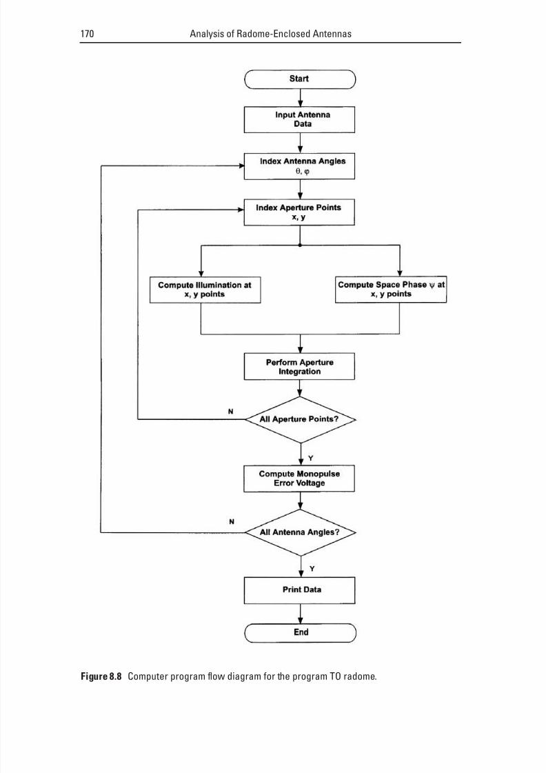
8/20/2019 Analysis of Radome-Enclosed Antennas
http://slidepdf.com/reader/full/analysis-of-radome-enclosed-antennas 191/319
170 Analysis of Radome-Enclosed Antennas
Figure 8.8 Computer program flow diagram for the program TO radome.

8/20/2019 Analysis of Radome-Enclosed Antennas
http://slidepdf.com/reader/full/analysis-of-radome-enclosed-antennas 192/319
Figure 8.10 depicts the corresponding azimuth and elevation plane monopulseerror channel voltages. Since there are no radome-induced errors, both of thesefunctions are zero on the antenna boresight. In performing this modeling, we
investigated the computational error in first sidelobe and antenna sum channelhalf-power beamwidth predictions versus the number of aperture sample pointsper wavelength. The resulting data are plotted in Figure 8.11 for sidelobe accu-racy in Figure 8.12 for antenna beamwidth computational accuracy.
8.3 Calculation of Radiation Patterns and Monopulse Error Voltagesfor an Antenna with a Radome
8.3.1 General ApproachThere are several approaches to boresight error computation:
1. Determine the shift in the difference pattern’s null position, whichresults from a wavefront phase distortion of the signal as it propagatesthrough the radome [16].
2. Determine the far-field sum pattern peak location [17].
This chapter uses the first method, which derives boresight error in thesame way that a monopulse seeker does. This method is based on the determina-tion of the shift in the zero crossings of the monopulse error in channel voltages
Radome-Enclosed Guidance Antennas 171
Figure 8.9 Computation of azimuth and elevation plane monopulse antenna sum pattern for
a 15-inch aperture at 10 GHz.
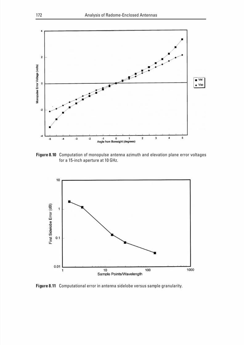
8/20/2019 Analysis of Radome-Enclosed Antennas
http://slidepdf.com/reader/full/analysis-of-radome-enclosed-antennas 193/319
172 Analysis of Radome-Enclosed Antennas
Figure 8.10 Computation of monopulse antenna azimuth and elevation plane error voltages
for a 15-inch aperture at 10 GHz.
Figure 8.11 Computational error in antenna sidelobe versus sample granularity.

8/20/2019 Analysis of Radome-Enclosed Antennas
http://slidepdf.com/reader/full/analysis-of-radome-enclosed-antennas 194/319
since the resulting wave diffraction with a radome causes a shift in the apparent
direction of the target.In (8.1) and (8.2), we showed how monopulse azimuth and elevationplane error voltages are derived from the monopulse antenna sum and differenceport voltages. When no radome is present, the zero crossings in these monopulseerror voltage channels correspond to the condition of a target on the antenna axis (i.e., normal to the surface of the antenna). With a radome over theantenna, as the electromagnetic signal propagates through the dielectric radome
wall, the resulting wave diffraction causes a shift in the apparent direction of thetarget.
With the antenna physically boresighted on the target, the azimuth andelevation boresight errors are computed from the following formulas [18]:
BSE V
K AZ
AZ
AZ
= (8.21)
BSE V
K
EL EL
EL
= (8.22)
In these equations, the constants K az and K el are the azimuth and elevationdifference channel monopulse antenna sensitivity constants, computed (or mea-sured) for the no-radome condition. Usually, these constants have units of
Radome-Enclosed Guidance Antennas 173
Figure 8.12 Computational error in antenna beamwidth versus sample granularity.
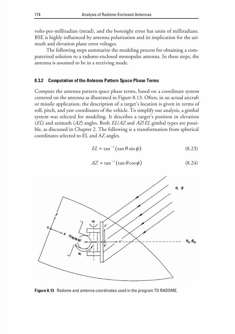
8/20/2019 Analysis of Radome-Enclosed Antennas
http://slidepdf.com/reader/full/analysis-of-radome-enclosed-antennas 195/319

8/20/2019 Analysis of Radome-Enclosed Antennas
http://slidepdf.com/reader/full/analysis-of-radome-enclosed-antennas 196/319
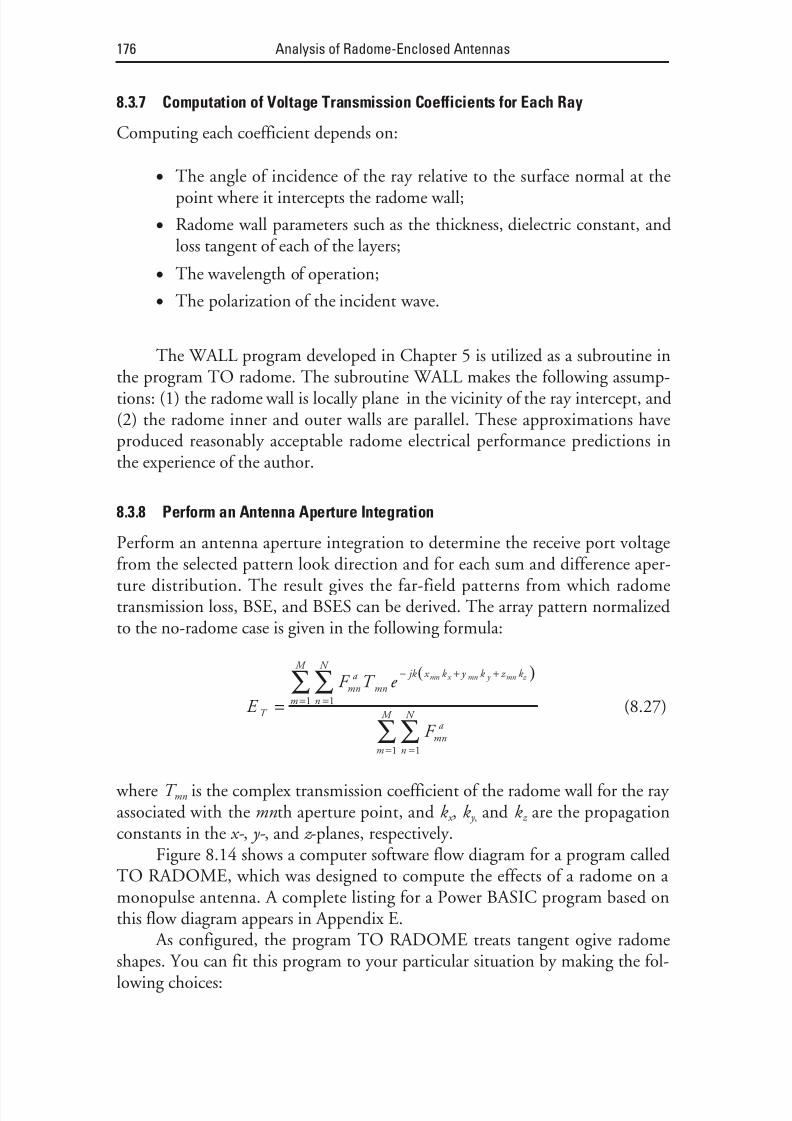
8/20/2019 Analysis of Radome-Enclosed Antennas
http://slidepdf.com/reader/full/analysis-of-radome-enclosed-antennas 197/319
8.3.7 Computation of Voltage Transmission Coefficients for Each Ray
Computing each coefficient depends on:
• The angle of incidence of the ray relative to the surface normal at thepoint where it intercepts the radome wall;
• Radome wall parameters such as the thickness, dielectric constant, andloss tangent of each of the layers;
• The wavelength of operation;
• The polarization of the incident wave.
The WALL program developed in Chapter 5 is utilized as a subroutine inthe program TO radome. The subroutine WALL makes the following assump-tions: (1) the radome wall is locally plane in the vicinity of the ray intercept, and(2) the radome inner and outer walls are parallel. These approximations haveproduced reasonably acceptable radome electrical performance predictions inthe experience of the author.
8.3.8 Perform an Antenna Aperture Integration
Perform an antenna aperture integration to determine the receive port voltagefrom the selected pattern look direction and for each sum and difference aper-ture distribution. The result gives the far-field patterns from which radometransmission loss, BSE, and BSES can be derived. The array pattern normalizedto the no-radome case is given in the following formula:
( )
E
F T e
F T
mn a
mn
jk x k y k z k
n
N
m
M
mn a
n
N
mn x mn y mn z
=
− + +
==
=
∑∑
∑11
1m
M
=∑
1
(8.27)
where T mn is the complex transmission coefficient of the radome wall for the ray associated with the mn th aperture point, and k x , k y , and k z are the propagationconstants in the x- , y- , and z -planes, respectively.
Figure 8.14 shows a computer software flow diagram for a program called
TO RADOME, which was designed to compute the effects of a radome on a monopulse antenna. A complete listing for a Power BASIC program based onthis flow diagram appears in Appendix E.
As configured, the program TO RADOME treats tangent ogive radomeshapes. You can fit this program to your particular situation by making the fol-lowing choices:
176 Analysis of Radome-Enclosed Antennas

8/20/2019 Analysis of Radome-Enclosed Antennas
http://slidepdf.com/reader/full/analysis-of-radome-enclosed-antennas 198/319
• Choose either AZ/EL or EL/AZ antenna gimbal configurations.
• Model the radome wall geometry up to 10 layers.
• Specify the thickness, dielectric constant, and loss tangent of each of these layers.
Radome-Enclosed Guidance Antennas 177
Figure 8.14 Computer software flow diagram for the program TO RADOME.

8/20/2019 Analysis of Radome-Enclosed Antennas
http://slidepdf.com/reader/full/analysis-of-radome-enclosed-antennas 199/319
8.4 Additional Modeling Considerations
This section discusses miscellaneous factors that may be necessary to model in a
given situation. The discussion that follows applies principally to radomes usedon airborne vehicles such as aircraft or missiles.
8.4.1 Rain Erosion of Missile Radomes
For high-speed flight through rain, significant radome material may erode fromthe outer wall, particularly in ceramic radome materials. To account for the wallthickness reduction, you must modify the radome wall thickness during the
modeling process. A relationship of the material eroded per unit area (T k ) for a fixed exposure time and the rain impingement angle d r (relative to the radomesurface normal) can be defined for many materials.
( )T K V k m r m = −
sin γ α 1
(8.28)
where V is the velocity in meters per second (m/s) and K m and αm are the con-stants for a particular material. For example, slip cast fused silica (SCFS), a pop-ular monolithic radome material, offers excellent thermal shock resistance andelectrical properties. However, it has poor rain erosion resistance above Mach 2[19]. Balageas has published an empirical formula to calculate the material ero-sion rate of SCFS based on simulation test results [20].
( ) ( )dT
dt D D C V K
r r r r = − +−10 3 67 6 78 3 949 2 6 3 5 3. . . sin. .
γ (8.29)
wheredT
k /dt = rate of material erosion (ìm/s);
D r = diameter of rain drop (mm);
C r = rain concentration (g/cm
3).
Equation (8.29) calculates the total erosion incurred by the radome by inputting velocity as a function of time on a flight path, and then integrating tofind the total material eroded.
Equations similar to the above model require a knowledge of rain data. A computerized environmental analysis technique has been developed to permitthe rapid evaluation of path-cumulative rainfall statistics. The analysis postulatesa generic thunderstorm of a circular cross section and varying vertical intensity.
At a selected altitude, the path-cumulative rainfall is evaluated along a path of arbitrary origin and direction. It is believed that this approach could provide a
178 Analysis of Radome-Enclosed Antennas

8/20/2019 Analysis of Radome-Enclosed Antennas
http://slidepdf.com/reader/full/analysis-of-radome-enclosed-antennas 200/319
much-needed means for quantitatively evaluating the rain environmentlimitations of tactical missile radomes [21].
For candidate radome materials, the erosion data can be obtained by test-
ing small samples on a high-speed sled through a manmade (simulated) rainfield. Tests reported in the technical literature have been at velocities up toapproximately Mach 5 (over 1 mile per second) [22]. Silicon nitride has beensled-tested in simulated rain to determine the influence of porosity and density on the response of this material to the rain droplet impact [23]. Variations of Duroid (a glass microfiber-loaded Teflon material) have been run in sled tests[24] to determine the optimum fiber type, content, and orientation for mini-mum aerothermal ablation and rain erosion.
Data published in the technical literature indicate that in the special case
of normal (or near-normal impact) that even with subsonic velocities it is neces-sary to put a rain erosion cap at the tip of the radome. This cap is usually metal-lic. To combine very high rain erosion resistance with good electrical properties,a dense silicon nitride cap obtained by hot pressed sintering has been employed,as described in [25]. In radome analysis modeling, an approximation of theeffects of a metallic nose cap can be obtained by nulling all rays that interceptthe nose cap (geometric optics approach).
8.4.2 Aerothermal Heating
For supersonic homing missiles whose mission includes the attack of supersonicmaneuvering targets at a high altitude, the guidance system absolutely requireshigh accuracy. As a result, the guidance engineer places a stringent requirementon the allowable boresight errors (BSE) caused by the radome. For this reason,many radomes are prescription ground prior to installation on the missileairframe [26].
The effects of aerodynamic heating are:
• A decrease in dielectric permittivity;
• An increase in loss tangent.
As a result, radome BSE, BSES, and losses increase with increasing radome wall temperature.
To model aerodynamic heating of the radome wall, it is often convenient
to express the temperatures over the entire surface of the radome as a function of the longitudinal position and as a function of the circumferential position.
Computer programs exist which determine temperatures of an aircraft ormissile radome due to aerodynamic heating. This heating is a function of trajec-tory, altitude profile, velocity, and maneuvers. One such program, URLIM
Radome-Enclosed Guidance Antennas 179

8/20/2019 Analysis of Radome-Enclosed Antennas
http://slidepdf.com/reader/full/analysis-of-radome-enclosed-antennas 201/319
[27], calculates temperatures for various points along a trajectory. It also com-putes the bending stresses at the base of the radome due to aerodynamic pressureand maneuver loads.
Thermal analysis theory is discussed in a report written by the Georgia Institute of Technology [27]. The approach generates temperature profilesthrough the radome material versus trajectory time. The model predicts theeffects of temperature changes on electromagnetic windows for single- and mul-tiple-layer windows. Temperature effects on expansion, complex permittivity,and complex permeability are included in the model. Performance factorsinclude transmission, reflection, insertion phase delay, and absorption as func-tions of the angle of incidence, polarization, and temperature for a flat-platesingle- or multiple-layer slab.
The philosophy followed by electromagnetic (EM) radome designers is toprovide a radome having low boresight errors at ambient temperature, but notat high temperatures [28]. Because radome-induced errors increase with temper-ature, if the magnitude of the boresight error is large enough, an oscillatory guidance system instability can result [29]. Compensation (filtering) within theguidance loop is possible to minimize the effects of the boresight error. How-ever, compensation decreases missile responsiveness and missile effectiveness.Missile instability may not necessarily result in significant performance degrada-
tion if the errors are confined to small regions of the radome [30].
8.4.3 Radome Effects on Conscan Antennas
Conical scan tracking systems (conscan) are generally less complex and lessexpensive than monopulse systems. Using conscan, a single antenna beam is off-set from the antenna axis and rotated about the antenna. For instance, consider
physically rotating an offset antenna reflector or antenna feed. The modulationsof a received signal within the antenna beamwidth are correlated with resolverson the scanning mechanism to determine the position of the target relative tothe antenna axis. Conscan was popular for use in small missiles.
Although conscan systems have simplicity and cost advantages relative tomonopulse systems, they also have performance deficiencies. For instance,because of the offset and beam nutation, the actual beamwidth of the antenna isup to 40% greater than the minimum beamwidth possible. In some cases, the
crossover of the beam is at the half-power point of the two-way antenna pattern.On an antenna boresight, a net loss results in about 3 dB of receive signal gain[10].
In comparing data for conscan antennas with monopulse antennas of thesame diameter and gimbal location within the same radome, the differences incomputed BSE and radome transmission loss are very small. Therefore, a
180 Analysis of Radome-Enclosed Antennas
8/20/2019 Analysis of Radome-Enclosed Antennas
http://slidepdf.com/reader/full/analysis-of-radome-enclosed-antennas 202/319
conscan antenna can be approximately modeled by a monopulse antenna of thesame diameter, using the techniques of this chapter.
References
[1] Dowsett, P. H., “Cross Polarization in Radomes: A Program for Its Computation,” IEEE Transactions on Aerospace Electronics Systems , Vol. AES-9, No. 3, May 1973, pp. 421–433.
[2] Huddleston, G. K., “Radomes,” Ch. 42 in Antenna Engineering Handbook , 3rd ed., R. C. Johnson, (ed.), New York: McGraw-Hill, 1992.
[3] Gulick, J. F., “Overview of Missile Guidance,” IEEE Eastcon Record , September 1978, pp.194–198.
[4] Sparks, R. A., “Systems Applications of Mechanically Scanned Slotted Array Antennas,”Microwave Journal , Vol.31, No. 6, June 1988, pp. 26–48.
[5] Lalezari, F., T. C. Boone, and J. M. Rogers, “Planar Millimeter Wave Arrays,” Microwave Journal , Vol. 34, No. 4, April 1991, pp. 85–92.
[6] Kelly, W., “Homing Missile Guidance—A Survey of Classical and Modern Techniques,”IEEE Southcon Technical Proceedings , January 1981.
[7] Savage, P. G., “A Strapdown Phased Array Radar Tracker Loop Concept for a Radar
Homing Missile,” AIAA Guidance Control Flight Conference , August 1969, pp. 1–8.[8] Schuchardt, M. J., and D. J. Kozakoff, “Seeker Antennas,” Ch. 38 in Antenna Engineering
Handbook , 3rd ed., R. C. Johnson, (ed.), New York: McGraw-Hill, 1992.
[9] Hirsch, H. L., and D. C. Grove, Practical Simulation of Radar Antennas and Radomes ,Norwood, MA: Artech House, 1987.
[10] Skolnik, M. I., Introduction to Radar Systems , 2nd ed., New York: McGraw-Hill, 1970.
[11] Huddleston, G. K., “Near Field Effects on Radome Boresight Errors,” Proceedings of the 17th Symposium on Electromagnetic Windows , Georgia Institute of Technology, Atlanta,
GA, July 1984, pp. 41–55.
[12] Hacker, P. S., and H. E. Schrank, “Range Distance Requirements for Measuring Low andUltra Low Sidelobe Antenna Patterns,” IEEE Transactions on Antennas and Propagation ,Vol. AP-30, No. 5, September 1982, pp. 956–965.
[13] Hansen, R. C., “Measurement Distance Effects on Low Sidelobe Patterns,” IEEE Transac- tions on Antennas and Propagation , Vol. AP-32, No. 6, June 1984, pp. 591–594.
[14] Mailloux, R. J., Phased Array Antenna Handbook , Norwood, MA: Artech House, 1994.
[15] Sokolnikoff, I. S., and R. M. Redheffer, Mathematics of Physics and Modern Engineering ,New York: McGraw-Hill, 1958.
[16] Hayward, R. A., E. L. Rope, and G. Tricoles, “Radome Boresight Error and Its Relation to Wavefront Distortion,” Proceedings of the 13th Symposium on Electromagnetic Windows ,Georgia Institute of Technology, Atlanta, GA, September 1976, pp. 87–92.
Radome-Enclosed Guidance Antennas 181

8/20/2019 Analysis of Radome-Enclosed Antennas
http://slidepdf.com/reader/full/analysis-of-radome-enclosed-antennas 203/319
[17] Siwiak, K., T. Dowling, and L. R. Lewis, “Numerical Aspects of Radome Boresight Error Analysis,” Proceedings of the 14th Symposium on Electromagnetic Windows , Georgia Insti-tute of Technology, Atlanta, GA, 1978.
[18] Schuchardt, J. M., et al., “Automated Radome Performance Evaluation in the Radio Fre-quency Simulation System (RFSS) Facility at MICOM,” Proceedings of the 15th Sympo- sium on Electromagnetic Windows , Georgia Institute of Technology, Atlanta, GA, June1980.
[19] Barta, J., “Rain and Sand Resistance of SCFS Radomes,” Proceedings of the 18th Sympo- sium on Electromagnetic Windows , Georgia Institute of Technology, Atlanta, GA, Septem-ber 1986, pp. 131–138.
[20] Balageas, D., and A. Hivert, “Rain Erosion, a Serious Problem for Slip Cast Fused Silica,”Proceedings of the 13th Symposium on Electromagnetic Windows , Georgia Institute of Tech-
nology, Atlanta, GA, September 1976, pp. 45–49.[21] Crowe, B. J., “Radome Rain Damage—An Environmental Analysis Technique,” Proceed-
ings of the 15th Symposium on Electromagnetic Windows , Georgia Institute of Technology, Atlanta, GA, June 1980.
[22] Frazer, R. K., “Rain Erosion Tests of Full Size Slip Cast Fused Silica Radomes at M3.5and M4.8,” Proceedings of the 17th Symposium on Electromagnetic Windows , Georgia Insti-tute of Technology, Atlanta, GA, July 1984.
[23] Schmitt, G. F., “Influence of Porosity and Density on the Supersonic Rain Erosion Behav-
ior of Silicon Nitride Radome Materials,” Proceedings of the 13th Symposium on Electro- magnetic Windows , Georgia Institute of Technology, Atlanta, GA, September 1976, pp.37–44.
[24] Bomar, S. H., et al., Materials Evaluation , Technical Report AFAL-TR-73-222, WrightPatterson Air Force Base, Dayton, OH; prepared by Georgia Institute of Technology,
Atlanta, GA, 1973.
[25] Letson, K. N., W. G. Burleson, and R. A. Reynolds, “Influence of Angle of Incidence onthe Rain Erosion Behavior of Duroid Radome Materials,” Proceedings of the 16th Sympo- sium on Electromagnetic Windows , Georgia Institute of Technology, Atlanta, GA, June
1982, pp. 181–186.
[26] Weckesser, L. B., et al., “Aerodynamic Heating Effects on Radome Boresight Errors,” Pro- ceedings of the 14th Symposium on Electromagnetic Windows , Georgia Institute of Technol-ogy, Atlanta, GA, June 1978.
[27] Frazer, R. K., “Use of the URLIM Computer Program for Radome Analysis,” Proceedings of the 14th Symposium on Electromagnetic Windows , Georgia Institute of Technology,
Atlanta, GA, June 1978, pp. 65–70.
[28] Kuehne, B. E., and D. J. Yost, “When Are Boresight Error Slopes Excessive?” Proceedings
of the 14th Symposium on Electromagnetic Windows , Georgia Institute of Technology, Atlanta, GA, June 1978.
[29] Jefferson, F. L., “Minimizing Effects of Temperature Changes on Electromagnetic Win-dows,” Proceedings of the 20th Symposium on Electromagnetic Windows , Georgia Institute of Technology, Atlanta, GA, September 1992, pp. 50–55.
182 Analysis of Radome-Enclosed Antennas

8/20/2019 Analysis of Radome-Enclosed Antennas
http://slidepdf.com/reader/full/analysis-of-radome-enclosed-antennas 204/319
[30] Weckesser, L. B., “Radome Aerodynamic Heating Effects on Boresight Error,” Proceedings of the 15th Symposium on Electromagnetic Windows , Georgia Institute of Technology,
Atlanta, GA, June 1980, pp. 97–101.
Selected Bibliography
Garnell, P., and D. J. East, Guided Weapons Control Systems , London, England: Pergamon Press,1977.
Hayward, R. A., E. L. Rope, and G. Tricoles, “Accuracy of Two Methods for Numerical Analysisof Radome Electromagnetic Effects,” Proceedings of the 14th Symposium on Electromagnetic Win- dows , Georgia Institute of Technology, Atlanta, GA, June 1978, pp. 53–57.
Huddleston, G. K., “Near-Field Effects on Radome Boresight Errors,” Proceedings of the 17th Symposium on Electromagnetic Windows, Georgia Institute of Technology , Atlanta, GA, July 1984,pp. 41–55.
Letson, K. N., et al., “Rain Erosion and Aerothermal Sled Test Results on Radome Materials,”Proceedings of the 14th Symposium on Electromagnetics Windows , Georgia Institute of Technology,
Atlanta, GA, June 1978, pp. 109–116.
Pendergrass, T. S., Radome Analysis , Technical Report AD-A136805, Huntsville, AL, TeledyneBrown Engineering, 1983.
Radome-Enclosed Guidance Antennas 183

8/20/2019 Analysis of Radome-Enclosed Antennas
http://slidepdf.com/reader/full/analysis-of-radome-enclosed-antennas 205/319

8/20/2019 Analysis of Radome-Enclosed Antennas
http://slidepdf.com/reader/full/analysis-of-radome-enclosed-antennas 206/319
9Miscellaneous Radome-EnclosedAntenna Types
Increasingly, radome-enclosed antennas are finding new applications in technol-ogy areas that include, but are not limited to, satellite navigation and communi-cations, telecommunications, and avionics. This chapter discusses radomeanalysis methods for the following situations: spiral antennas, parabolas and
other telecommunications antennas, air-supported radomes, metal space frameradomes, and radome-enclosed phased-array antennas.
9.1 Spiral Antennas
9.1.1 Single Mode Spiral Antennas
A planar spiral antenna as illustrated in Figures 9.1 and 9.2 is a very broadband,circularly polarized antenna element. Planar spirals are popular for use inantiradiation homing (ARH) missile guidance systems [1] or in electronicscountermeasures (ECM) direction-finding systems on aircraft. A complete dis-cussion of this category of antennas appeared in Chapter 3.
Spiral antennas typically use printed circuit technology. However, thislimits their use to low-power transmit or receive applications. Thus, spirals areusually used for passive applications. Current tolerances obtained with this typeof fabrication technology permit spiral electrical operation to at least Ka-bandon the high end of the spectrum. Spiral antennas are available to at least L-band
on the low end of the spectrum. Furthermore, certain loading techniques canreduce size or permit operation at even lower frequencies [2].
185

8/20/2019 Analysis of Radome-Enclosed Antennas
http://slidepdf.com/reader/full/analysis-of-radome-enclosed-antennas 207/319
The typical antenna half-power beamwidth (HPBW) is up to 90°. This wide, instantaneous field of view makes these antennas attractive for many body fixed missile guidance applications [3]. Spiral antennas can by used in arrays of two or more elements in small interferometers [4]. Missile guidance systemsusing these are usually fixed-mounted (nongimbaled) with pursuit navigationalgorithms to obtain line-of-sight data to the target [5]. Figure 9.3 illustratesseveral array geometries for reference.
186 Analysis of Radome-Enclosed Antennas
Figure 9.1 A broadband, cavity-backed, planar Archimedean spiral antenna. (Photo cour-
tesy of Tracor Aerospace Electronic Systems.)
(a) (b)
Figure 9.2 Lower microwave frequency spiral antenna and plastic radome. (Photo courtesy
of USDigiComm Corporation.)

8/20/2019 Analysis of Radome-Enclosed Antennas
http://slidepdf.com/reader/full/analysis-of-radome-enclosed-antennas 208/319
For the no-radome condition, the principal plane sum and difference pat-terns for the two-element, spiral antenna array are given by the following formulas:
Σ =
cos sin cos
π
λθ θ
d a
o
(9.1)
∆ =
sin sin cos
π
λθ θ
d a
o
(9.2)
where
θ = angle measured from the antenna boresight;
d a = center-to-center spacing between the two spiral antennas;
λo = the operating wavelength in free space.
Figure 9.4 shows a microwave circuit to resolve the received antenna sig-nals from a four-element spiral array into monopulse sum and differencepatterns.
Placing a radome over a spiral antenna array results in an apparentboresight error (BSE) because of the wavefront phase modification over theantenna apertures. These effects need to be carefully considered during the selec-tion of a radome design since they will influence the seeker system accuracy per-formance [6–8]. Broadband ARH or ECM antennas generally require
Miscellaneous Radome-Enclosed Antenna Types 187
Figure 9.3 Spiral antenna array geometries.

8/20/2019 Analysis of Radome-Enclosed Antennas
http://slidepdf.com/reader/full/analysis-of-radome-enclosed-antennas 209/319

8/20/2019 Analysis of Radome-Enclosed Antennas
http://slidepdf.com/reader/full/analysis-of-radome-enclosed-antennas 210/319
The following method is useful for estimating the BSE characteristics of the spiral antenna array. From Figure 9.4, rewrite the monopulse sum and dif-ference formulas to incorporate a radome transmission coefficient associated
with each antenna, based on the simple ray trace depicted in Figure 9.5.
( ) ( )Σ = + + +T A T A T A T A w w w w 1 1 2 2 3 3 4 4 (9.3)
( ) ( )∆ az w w w w T A T A T A T A = + − +1 1 2 2 3 3 4 4
(9.4)
( ) ( )∆ el w w w w T A T A T A T A = − +1 1 3 3 2 2 4 3_ (9.5)
In these equations, the signal amplitudes of each of the spiral antennas, A i ,are normally all about equal. However, the phase associated with each varies inthe array. The transmission coefficients, T wi , can be evaluated by the wall con-struction, material properties, polarization, wavelength, and the angle of inci-dence of a ray with respect to the surface normal at the intercept point.
A more accurate method of obtaining estimates of radome impact on theperformance of the spiral array is based on equivalent transmission coefficients.
Assuming a receive mode, the surface integration shown in Figure 9.6 illustrates
the method. The procedure involves the physical optics (PO) method discussed
Miscellaneous Radome-Enclosed Antenna Types 189
Figure 9.5 Simple ray trace.

8/20/2019 Analysis of Radome-Enclosed Antennas
http://slidepdf.com/reader/full/analysis-of-radome-enclosed-antennas 211/319
in Section 6.3, which models an incoming plane wavefront as an ensemble of Huygens’ sources. The external reference plane is used to transform points fromthe ensemble of Huygens’ sources to a point centered on each spiral antenna aperture [11]. In other words, we trace rays coming from points on the external
reference plane, incorporating the radome transmission coefficient to modify each ray. From this process, we derive an equivalent transmission coefficient in a given look direction θ, φ.
( )( )T
MN
T
r r e mn
mn o
jk r r
n
N
m
M mn o = − −
==∑∑1
0
11
(9.6)
where the m and n indices correspond to points on the external reference plane.
9.1.2 Multimode Spiral Antennas
If the diameter of a spiral antenna is sufficiently large, higher-order modes may exist. These correspond to active ring circumferences corresponding to P λ for theP th mode, where P is an integer. The electrical phase of the currents on these
190 Analysis of Radome-Enclosed Antennas
Figure 9.6 Reference plane and ray trace technique to obtain an equivalent transmission
coefficient.
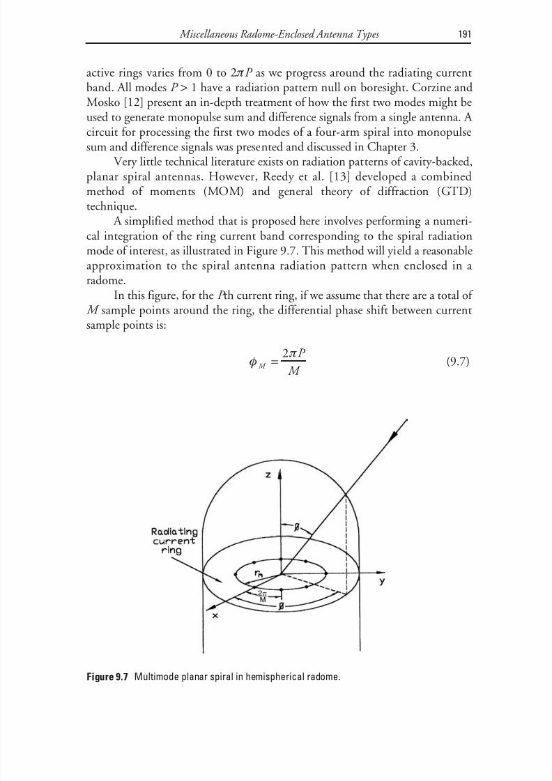
8/20/2019 Analysis of Radome-Enclosed Antennas
http://slidepdf.com/reader/full/analysis-of-radome-enclosed-antennas 212/319
active rings varies from 0 to 2 πP as we progress around the radiating currentband. All modes P > 1 have a radiation pattern null on boresight. Corzine andMosko [12] present an in-depth treatment of how the first two modes might be
used to generate monopulse sum and difference signals from a single antenna. A circuit for processing the first two modes of a four-arm spiral into monopulsesum and difference signals was presented and discussed in Chapter 3.
Very little technical literature exists on radiation patterns of cavity-backed,planar spiral antennas. However, Reedy et al. [13] developed a combinedmethod of moments (MOM) and general theory of diffraction (GTD)technique.
A simplified method that is proposed here involves performing a numeri-cal integration of the ring current band corresponding to the spiral radiation
mode of interest, as illustrated in Figure 9.7. This method will yield a reasonableapproximation to the spiral antenna radiation pattern when enclosed in a radome.
In this figure, for the P th current ring, if we assume that there are a total of M sample points around the ring, the differential phase shift between currentsample points is:
φ π
M
P
M =
2(9.7)
Miscellaneous Radome-Enclosed Antenna Types 191
Figure 9.7 Multimode planar spiral in hemispherical radome.

8/20/2019 Analysis of Radome-Enclosed Antennas
http://slidepdf.com/reader/full/analysis-of-radome-enclosed-antennas 213/319
and the phase shift at sample point m is:
φ φ π
m M m mP
M
= = 2
(9.8)
The array factor for the P th current ring is then broken into φ and θ fieldcomponents:
( )E m
M e T e x
AF j m
jk x y m m = −
− +sin , sin cos2 π
θ φ φ θ φ( )m
m
N sin sinθ φ
=∑
0
(9.9)
( )E m M
e T e y AF j
m jk x y m m m = − +cos , sin cos2 π θ φ φ θ φ( )sin sinθ φ
m
N
=∑0
(9.10)
In (9.9) and (9.10), the following definitions apply.
T m (θ, φ) = complex radome wall voltage transmission coefficient associ-
ated with the m th sample point for a ray incident from the θ, φ direction;
x m = x coordinate of the m th point on the P th current ring (m) = r p cos ϕm ;
Y m = y coordinate of the m th point on the P th current ring (m) = r p sin ϕm ;r p = radius of P th current ring (m) = P λ
π2.
9.2 Large Parabolic Antennas
Since World War II, the number of telecommunications antenna radomes hassteadily increased. As the advantages of radomes become more widely recog-
nized, the rate at which radomes are added continues to grow. To meet thisgrowing need, it is important that specific analysis techniques be developed fortelecommunications radomes.
For telecommunications antennas such as parabolas, generally a planarfabric or membrane radome is used, as illustrated in Figure 9.8. These radomesare electrically thin. The losses are held low by using a thin, low-loss materialsuch as Teglar, a fiberglass material coated on both sides with Teflon that sheds
water readily [14].
Because of their close proximity to the antenna feed, these planar radomescan introduce small increases in the antenna voltage standing wave ratio(VSWR) [15]. For a planar radome like the one shown in Figure 9.8, the VSWR increase can be reduced by tilting the radome a few degrees (moving the top fur-ther from an antenna aperture) to prevent a specular return to the feed horn[16].
192 Analysis of Radome-Enclosed Antennas
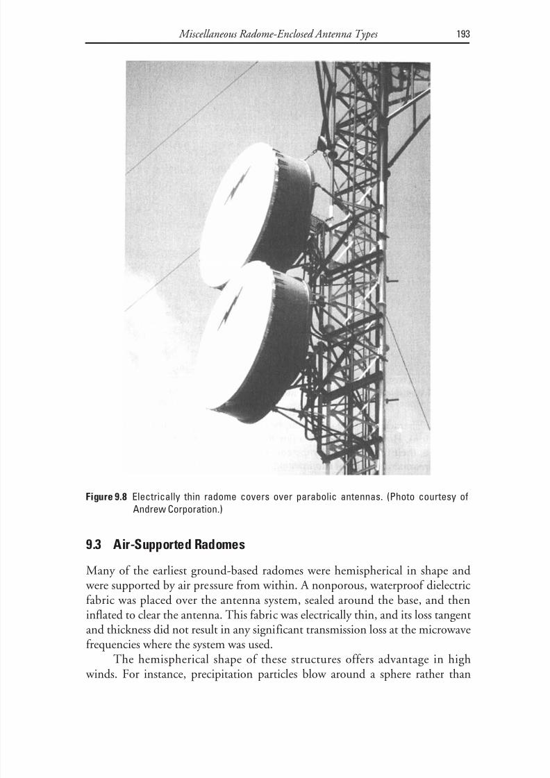
8/20/2019 Analysis of Radome-Enclosed Antennas
http://slidepdf.com/reader/full/analysis-of-radome-enclosed-antennas 214/319
9.3 Air-Supported Radomes
Many of the earliest ground-based radomes were hemispherical in shape and were supported by air pressure from within. A nonporous, waterproof dielectricfabric was placed over the antenna system, sealed around the base, and then
inflated to clear the antenna. This fabric was electrically thin, and its loss tangentand thickness did not result in any significant transmission loss at the microwavefrequencies where the system was used.
The hemispherical shape of these structures offers advantage in high winds. For instance, precipitation particles blow around a sphere rather than
Miscellaneous Radome-Enclosed Antenna Types 193
Figure 9.8 Electrically thin radome covers over parabolic antennas. (Photo courtesy of
Andrew Corporation.)

8/20/2019 Analysis of Radome-Enclosed Antennas
http://slidepdf.com/reader/full/analysis-of-radome-enclosed-antennas 215/319
impinge upon it. Therefore, snow, frozen precipitation, or rain is not readily deposited on the spherical surface. With these radome shapes, the incidenceangles are usually less than 30°. Such radomes are called normal incidence
radomes [17]. The transmission properties of wall structures commonly used inthis type of radome are relatively independent on polarization and incidenceangles between 0° and 30°, particularly if small tolerances on thickness varia-tions are maintained and a narrow frequency band of operation is specified.
Early materials used for air-supported radomes were neoprene-coatednylon, hypalon-coated Dacron, and Teflon-coated fiberglass [18]. Hemispheri-cal air-supported radomes greater that 70m in diameter are in service today [19].
The advantages of air-supported radomes are:
• Low cost;
• Good electromagnetic transparency over very wide frequency bandwidths;
• Relative ease of erection and dismantling.
These characteristics make air-supported radomes particularly suitable formobile stations. However, there are a few disadvantages to air-supportedradomes. For instance, their life is limited by the constant flexing of the materialin the wind. Furthermore, maintenance of the internal pressure in high windscan be difficult. Maintenance is costly and required at frequent intervals for theoverall structure and air pressure system.
Since air-supported radomes are electrically thin, monolithic wall struc-tures, the analysis for transmission loss can readily be done using the
WALL computer code discussed in Chapter 5. Other than transmission loss,these radomes generally have a negligible effect on antenna sidelobes or
depolarization.
9.4 Metal Space Frame Radomes
Rigid, self-supporting, space frame radomes overcome many limitations of air-supported radomes. As illustrated in Figure 9.9, these radomes consist of a three-dimensional lattice of primary, load-bearing, metallic members, which
carry the main loads or stresses. The framework is typically steel or aluminummembers. This type of design is sometimes called a geodesic dome , in which a spherical structure is built from simple geometrical shapes. Geodesic domedesign computer software is available in the form of DOME, a freeware DOSutility developed for generating the coordinates of a geodesic dome or sphere[20]. This zip archive includes DOS executable C++ source code. Of all the
194 Analysis of Radome-Enclosed Antennas
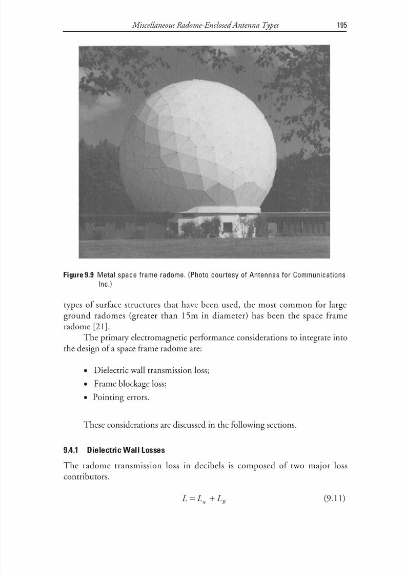
8/20/2019 Analysis of Radome-Enclosed Antennas
http://slidepdf.com/reader/full/analysis-of-radome-enclosed-antennas 216/319

8/20/2019 Analysis of Radome-Enclosed Antennas
http://slidepdf.com/reader/full/analysis-of-radome-enclosed-antennas 217/319

8/20/2019 Analysis of Radome-Enclosed Antennas
http://slidepdf.com/reader/full/analysis-of-radome-enclosed-antennas 218/319
In (9.13), we define the optical blockage function via the next formula:
( )G
A
A A A
A
η η η η
η=
− −−sin 1 2
2
1(9.14)
This optical blockage function is plotted in Figure 9.10.
9.4.3 Pointing Errors
The pointing errors introduced by space frame radomes are extremely small,usually less than 0.1 mrad.
A uniform space frame geometry theoretically can produce no boresighterror (BSE). As the geometry departs from perfect uniformity, the first signifi-cant effect is boresight error. For well-designed radomes, this appears to be theonly significant effect. Boresight errors can result from: (1) imperfect uniformity of the space frame geometry as designed, and/or (2) tolerance or manufacturing variations.
To minimize the BSE pattern distortion of the main lobe and close-insidelobes, the metallic frame geometry should have two characteristics:
Miscellaneous Radome-Enclosed Antenna Types 197
Figure 9.10 Dielectric space frame radome. (Photo courtesy of Antennas for Communica-
tions Inc.)

8/20/2019 Analysis of Radome-Enclosed Antennas
http://slidepdf.com/reader/full/analysis-of-radome-enclosed-antennas 219/319
• Be as uniform as possible. In other words, the blocking area ratioshould be the same in all parts of the radome. The blocking area geome-try shown in Figure 9.11 is one that achieves the latter requirement
quite effectively [22]• Be as random as possible. The more random the space frame geometry,
the less the BSE.
9.5 Dielectric Space Frame Radomes
The framework of a dielectric space frame radome typically consists of plastic, as
opposed to steel or aluminum members. These radomes have several advantagesover other ground-based radome types. The radome walls may be constructed asa thin membrane, a solid laminate, or a multilayer sandwich with internal foamcores. For the thin membrane wall, the radome panel flanges have dimensionscapable of supporting the environmental wind loads. Often a two- or three-layersandwich wall is used where thermal insulation or high-frequency and low-fre-quency loss requirements prevail.
The dielectric beams or struts act as dielectric loads. The radome engineercan add inductive elements to impedance-match a capacitive circuit load overthe required bandwidth. These inductive elements might be implemented via metalized elements dispersed into the radome panel fabric or wall material. Theresulting design provides reduced overall radome transmission loss, compared to
what can be achieved with a metal frame radome [23]. Figure 9.12 shows typicaldata comparing the transmission loss of a metal space frame radome with a dielectric space frame radome of the same size and construction.
198 Analysis of Radome-Enclosed Antennas
Figure 9.11 Optical blockage function versus antenna-radome diameter ratio [21].

8/20/2019 Analysis of Radome-Enclosed Antennas
http://slidepdf.com/reader/full/analysis-of-radome-enclosed-antennas 220/319
9.6 Radome Enclosed Phased-Array Antennas
For a phased-array antenna, the total antenna pattern can be expressed as a product of the element antenna pattern and an array factor:
( ) ( )E E E e AF θ φ θ φ, ,= (9.15)
The most commonly used element radiators for phased-array antennas areas follows:
• Dipoles;
• Slots in waveguide;
• Open-ended waveguides;
• Small horn antennas;
• Spiral antennas;
Miscellaneous Radome-Enclosed Antenna Types 199
Figure 9.12 Projection of the radome frame onto the antenna aperture [22].
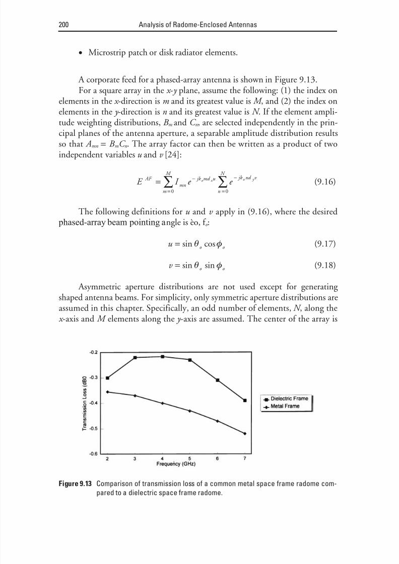
8/20/2019 Analysis of Radome-Enclosed Antennas
http://slidepdf.com/reader/full/analysis-of-radome-enclosed-antennas 221/319
• Microstrip patch or disk radiator elements.
A corporate feed for a phased-array antenna is shown in Figure 9.13.
For a square array in the x - y plane, assume the following: (1) the index onelements in the x -direction is m and its greatest value is M , and (2) the index onelements in the y -direction is n and its greatest value is N . If the element ampli-tude weighting distributions, B m and C n , are selected independently in the prin-cipal planes of the antenna aperture, a separable amplitude distribution resultsso that A mn = B m C n . The array factor can then be written as a product of twoindependent variables u and v [24]:
E I e e AF mn
jk md u
m
M jk nd v
n
N o x o y = −
=
−
=∑ ∑0 0
(9.16)
The following definitions for u and v apply in (9.16), where the desired phased-array beam pointing angle is èo, f o :
u o o = sin cosθ φ (9.17)
v o o = sin sinθ φ (9.18)
Asymmetric aperture distributions are not used except for generating shaped antenna beams. For simplicity, only symmetric aperture distributions areassumed in this chapter. Specifically, an odd number of elements, N , along thex -axis and M elements along the y -axis are assumed. The center of the array is
200 Analysis of Radome-Enclosed Antennas
Figure 9.13 Comparison of transmission loss of a common metal space frame radome com-
pared to a dielectric space frame radome.
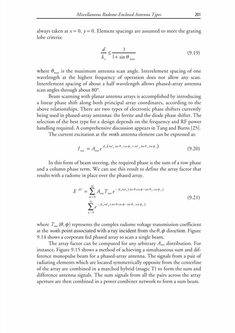
8/20/2019 Analysis of Radome-Enclosed Antennas
http://slidepdf.com/reader/full/analysis-of-radome-enclosed-antennas 222/319

8/20/2019 Analysis of Radome-Enclosed Antennas
http://slidepdf.com/reader/full/analysis-of-radome-enclosed-antennas 223/319
The desired amplitude distribution for the sum beam can be achieved by proper weighting of the signals in the combiner network. The difference signalsfrom all the pairs are combined in a separate power combiner network in orderto form a difference beam. Amplitude weighting in the two combiner networkscan take several forms to obtain low sidelobes for both the sum and the differ-ence antenna beams. For instance, a Bayliss type of distribution produces low
202 Analysis of Radome-Enclosed Antennas
Figure 9.14 Corporate feed for a phased-array antenna.
Figure 9.15 Phased-array monopulse feed.

8/20/2019 Analysis of Radome-Enclosed Antennas
http://slidepdf.com/reader/full/analysis-of-radome-enclosed-antennas 224/319
sidelobes for a difference beam [26]. For a cosq type of sum channel distribution,for a square array the first sidelobes correspond to −23 dB and −32 dB for q equal to 1 and 2, respectively.
References
[1] Dyson, J. D., “Multimode Logarithmic Spiral Antennas,” National Electronics Conference ,Vol. 17, October 1961, pp. 206–213.
[2] Morgan, T. E., “Reduced Size Spiral Antenna,” IEEE Ninth European Microwave Confer- ence Proceedings , September 1979, pp. 181–185.
[3] Schuchardt, J. M., D. J. Kozakoff, and M. Hallum, “Seeker Antennas,” Ch. 38 in Antenna Engineering Handbook , 2nd ed., R. C. Johnson and H. Jasik, (eds.), New York:McGraw-Hill, 1988.
[4] Schuchardt, J. M., and W. O. Purcell, “A Broadband Direction Finding Receiving Sys-tem,” Martin Marietta Interdivision Antenna Symposium , Orlando, FL, August 1967, pp.1–14.
[5] Feagler, E. R., “The Interferometer as a Sensor for Missile Guidance,” IEEE Eastcon Record , September 1978, pp. 203–210.
[6] Marales, G., “Simulation of Electrical Design of Streamlined Radomes,” AIAA Summer Computer Simulation Conference , Toronto, Canada, July 1979, pp. 353–354.
[7] Ossin, A., Millimeter Wavelength Radomes , Report AFML-TR-79-4076, Wright Patterson Air force Base, Dayton, OH, July 1979.
[8] Siwak, K., et al., “Boresight Errors Induced by Missile Radomes,” IEEE Transactions on Antennas and Propagation , Vol. AP-27, November 1979, pp. 832–841.
[9] Russell, R. F., and S. Massey, “Radio Frequency System Simulator,” AIAA Guidance Con- ference , August 1972, pp. 72–861.
[10] Sutherlin, D. W., and C.L. Phillips, “Hardware-in-the-Loop Simulation of AntiradiationMissiles,” IEEE Southeastcon Proceedings , Clemson, SC, April 1976, pp. 43–45.
[11] Israel, M., et al., “A Reference Plane Method for Antenna Radome Analysis,” Proceedings of the 15th Symposium on Electromagnetics Windows , Georgia Institute of Technology,
Atlanta, GA, 1980.
[12] Corzine, R. G., and J. A. Mosko, Four Arm Spiral Antennas , Norwood, MA, ArtechHouse, 1990.
[13] Reedy, C. J., M. D. Deshpande, and D. T. Fraleeh, Analysis of Elliptically Polarized Cavity
Backed Antennas Using a Combined FEM/MOM/GTD Technique , NASA CR 198197, August 1995.
[14] Sellar, C. A., Jr., “Preliminary Testing of Teflon as a Hydrophobic Coating for MicrowaveRadomes,” IEEE Transactions on Antennas and Propagation , Vol.AP-27, No. 4, July 1979,pp. 555–557.
Miscellaneous Radome-Enclosed Antenna Types 203
8/20/2019 Analysis of Radome-Enclosed Antennas
http://slidepdf.com/reader/full/analysis-of-radome-enclosed-antennas 225/319
[15] Redheffer, R. M., The Interaction of Microwave Antennas with Dielectric Sheets , RadiationLaboratory Report 484-18, Boston, MA, MIT Lincoln Laboratory, March 1946.
[16] Knop, C. M., “Microwave Relay Antennas,” Ch. 30 in Antenna Engineering Handbook ,3rd ed., R. C. Johnson, (ed.), New York: McGraw-Hill, 1993.
[17] Huddleston, G. K., and H. H. Bassett, “Radomes,” Ch. 44 in Antenna Engineering Hand- book , 3rd ed., R. C. Johnson, (ed.), New York: McGraw-Hill, 1993.
[18] Skolnik, M. I., Introduction to Radar Systems , 2nd ed., New York: McGraw-Hill, 1994.
[19] Bird, W. W., “Large Air Supported Radomes for Satellite Communications Ground Sta-tions,” Proceedings of the OSU-RTD Symposium on Electromagnetic Windows , Ohio StateUniversity, 1964.
[20] Bono, R., “Geodesic Domes,” http://www.cris.com/~rjbono/html/domes.html, 1996.
[21] D’Amato, R., “Metal Space Frame Radome Design,” International Symposium on Struc- tures Technology for Large Radio and Radar Telescope Systems , Massachusetts Institute of Technology, October 1967.
[22] Kay, A. L., “Electrical Design of Metal Space Frame Radomes,” IEEE Transactions on Antennas and Propagation , Vol. AP-13, March 1965.
[23] Dielectric Space Frame (DSF) Radome Advantages, Antennas for Communication (AFC)Company, ttp://www.ocala.com/afc/imp_mat.gif, 2009.
[24] Rudge, A. W., et al., A Handbook of Antenna Design , London, England: Peter PeregrinusLtd., 1986.
[25] Tang, R., and R. W. Burns, “Phased Arrays,” Ch. 20 in Antenna Engineering Handbook ,3rd ed., R. C. Johnson, (ed.), New York: McGraw-Hill, 1993.
[26] Bayliss, E. T., “Design of Monopulse Difference Patterns with Low Sidelobes,” Bell Sys- tems Technical Journal , May-June 1968, pp. 623–650.
Selected Bibliography
Bird, W. W., “Large Air Supported Radomes for Satellite Communications Ground Stations,”Proceedings of the OSU-RTD Symposium on Electromagnetic Windows , Ohio State University,1964.
Schuchardt, J. M., et al., “Automated Radome Performance Evaluation in the RFSS Facility atMICOM,” Proceedings of the 15th Electromagnetic Windows Symposium , Georgia Institute of Technology, Atlanta, GA, June 1980.
Webb, L. L., “Analysis of Field-of-View Versus Accuracy for a Microwave Monopulse,” IEEE
Southeascon Proceedings , April 1973, pp. 63–66.
204 Analysis of Radome-Enclosed Antennas

8/20/2019 Analysis of Radome-Enclosed Antennas
http://slidepdf.com/reader/full/analysis-of-radome-enclosed-antennas 226/319
Part IVRadome Specifications andEnvironmental Degradations

8/20/2019 Analysis of Radome-Enclosed Antennas
http://slidepdf.com/reader/full/analysis-of-radome-enclosed-antennas 227/319

8/20/2019 Analysis of Radome-Enclosed Antennas
http://slidepdf.com/reader/full/analysis-of-radome-enclosed-antennas 228/319
10Specifying and Testing RadomePerformance
10.1 Specifying Aircraft Radomes
The RTCA document DO-213 [1] gives an interesting overview of earlier mini-mal operational performance requirements for aircraft radomes used to encloseDoppler weather radar antennas. Therein, radome transmission efficiency isdefined as the one way that power transmission loss is expressed in percentage.For the various radome classes discussed earlier in this book, the average andminimum radome transmission efficiencies are as shown in Table 10.1.
The maximum radome BSE over the allowable scan angles of the antenna is specified as 8.72 mrad, the increase in beamwidth of the antenna is not toincrease by more than 10%, and the power reflected back into the antenna by the radome is not to exceed 0.5%.
10.2 Specifying Radomes for Terrestrial and Marine SATCOMAntennas
The satellite receives uplink signals, optionally processes these signals, translatesthem in frequency, and amplifies and retransmits these signals to another satel-lite or to one or more earth terminals. Besides normal requirements for low radome loss (−0.5-dB goal), for SATCOM use there are three special problemsthe designer will encounter:
207

8/20/2019 Analysis of Radome-Enclosed Antennas
http://slidepdf.com/reader/full/analysis-of-radome-enclosed-antennas 229/319
• Small radome depolarization to not degrade frequency reuse perfor-mance (as small as −40- to −50-dB radome depolarization sometimesrequired);
• Small registration error (difference between uplink and downlink BSE)that establishes the transmit beam direction based on the direction of the arrival beam;
• Very small, far-out sidelobes to conform to sidelobe envelope specifica-
tions appearing in FCC Part 25.209 regulations, Intelsat IESS-207 andIESS-601, Eutelsat EESS500, and so forth.
The key requirements for radomes enclosing SATCOM antennas are cov-ered in MIL-R-7705B [2], MIL-STD-188-146 [3], and by Lida [4], Kolawole[5], Tirro [6], and Evans [7].
10.3 Radome Testing Methodology
Radome electrical characterization testing is obviously required during thedesign and development stage of new aircraft radomes. However, electrical test-ing is also required for after the repair of radome defects according to Interna-tional standards as well as the aircraft manufacturers’ component maintenancemanuals. The following sections detail testing methods and general test equip-ment that is required in order to accomplish these tests and that is derived from
Fordham [8], Hartman [9], and Hollis et al. [10].
10.3.1 Outdoor Test Facilities
Radome tests performed on outdoor far-field ranges are normally in the very farfield where
208 Analysis of Radome-Enclosed Antennas
Table 10.1
Aircraft Radome Transmission Efficiency
Radome
Class
Average
Transmission
Efficiency
Minimum
Transmission
Efficiency
a 90% 85%
b 87% 82%
c 84% 78%
d 80% 75%
e 70% 55%

8/20/2019 Analysis of Radome-Enclosed Antennas
http://slidepdf.com/reader/full/analysis-of-radome-enclosed-antennas 230/319
R D
≥ 2 2
λ
where D is the diameter of the largest antenna and λ is the free space wavelengthcomputed at the test frequency.
In an outdoor far-field range configuration, the test antenna within theradome under test is normally installed on a test positioner located on a tower,roof, or platform outside the instrumentation control room. The microwavereceiver front end is usually located at the base of this test positioner, thereby requiring only a single RF path through the positioner, greatly simplifying sys-tem design. This setup as used for BSE or radome loss measurements is illus-
trated in Figure 10.1.For multiported antennas, for instance, a monopulse antenna having a sum channel and azimuth and elevation difference channels, simultaneous mea-surements can be made on all ports using multiplexers. The receiver front end isremotely controlled from the control console through interfaces with thereceiver.
Often, the position of the radome is electronically mechanically controlledaround the fixed receive antenna. The radome test positioner axes are read out
Specifying and Testing Radome Performance 209
Figure 10.1 Test setup for radiation pattern and BSE measurements.
8/20/2019 Analysis of Radome-Enclosed Antennas
http://slidepdf.com/reader/full/analysis-of-radome-enclosed-antennas 231/319
by positioner control and readout units. A typical control system consists of a control unit located in the operator’s console interfaced to a power amplifierunit located near the test positioner. This configuration keeps the high power
signals away from sensitive measurement instruments while providing a remotecontrol of positioner functions from the equipment console.The transmit antenna is normally located at the opposite end of the out-
door far-field antenna range on a tower or other supporting structure. The fre-quency synthesized signal source is installed near the transmit antenna tominimize signal loss. For some applications a multiplexer can be used betweenthe signal source and a dual polarized transmit antenna allowing simultaneouscopolarization and cross-polarization measurements to be performed. Utmostattention must be paid to test procedures and measurement sequences. After the
measurements are completed, most modern radome test facilities will automati-cally generate a test report for documentation purposes.
An equipment test setup for measuring radome-induced antenna VSWR isshown in Figure 10.2. This can also be easily implemented in an outdoor facility free and clear from reflections from objects in the vicinity of the measurements.
10.3.2 Use of Indoor Anechoic Chambers
According to RTCA DO-213 [1] for indoor anechoic chambers, the minimumrange distance R between the transmitting signal source and the receiving antenna as illustrated in Figure 10.3 shall be
R D ≥
2
2 λ
where D is the diameter of the largest antenna and λ is the free space wavelength
computed at the test frequency. This is generally not as good as what is obtain-able on outdoor antenna test ranges. Indoor anechoic chamber facilities are gen-erally extremely compact (chamber size 5-m length × 5-m width × 10-m depth)and can handle most aircraft radomes used in the industry.
The tests performed in these indoor anechoic chambers are transmissionefficiency, sidelobe level increase, and radome BSE. The procedure and equip-ment operation using modern test equipment is most often completely auto-mated, so that an electronics technician is normally the only skill level requiredto operate an indoor anechoic chamber radome test facility. For instance, in Fig-ure 10.4 a special automated positioner is seen, which allows the radome to bemoved around a fixed antenna. A photo of a radome loss measurement in pro-cess in an indoor anechoic chamber facility is shown in Figure 10.5.
210 Analysis of Radome-Enclosed Antennas

8/20/2019 Analysis of Radome-Enclosed Antennas
http://slidepdf.com/reader/full/analysis-of-radome-enclosed-antennas 232/319
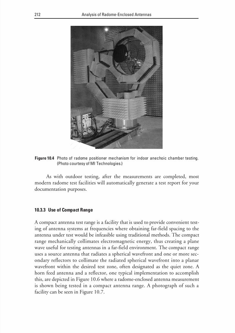
8/20/2019 Analysis of Radome-Enclosed Antennas
http://slidepdf.com/reader/full/analysis-of-radome-enclosed-antennas 233/319
As with outdoor testing, after the measurements are completed, mostmodern radome test facilities will automatically generate a test report for yourdocumentation purposes.
10.3.3 Use of Compact Range
A compact antenna test range is a facility that is used to provide convenient test-ing of antenna systems at frequencies where obtaining far-field spacing to theantenna under test would be infeasible using traditional methods. The compactrange mechanically collimates electromagnetic energy, thus creating a plane
wave useful for testing antennas in a far-field environment. The compact rangeuses a source antenna that radiates a spherical wavefront and one or more sec-
ondary reflectors to collimate the radiated spherical wavefront into a planar wavefront within the desired test zone, often designated as the quiet zone. A horn feed antenna and a reflector, one typical implementation to accomplishthis, are depicted in Figure 10.6 where a radome-enclosed antenna measurementis shown being tested in a compact antenna range. A photograph of such a facility can be seen in Figure 10.7.
212 Analysis of Radome-Enclosed Antennas
Figure 10.4 Photo of radome positioner mechanism for indoor anechoic chamber testing.(Photo courtesy of MI Technologies.)

8/20/2019 Analysis of Radome-Enclosed Antennas
http://slidepdf.com/reader/full/analysis-of-radome-enclosed-antennas 234/319
Specifying and Testing Radome Performance 213
Figure 10.5 Photo of radome loss measurement in an indoor anechoic chamber. (Photocourtesy of Saint-Gobain Performance Plastics.)
Figure 10.6 Facility for radome measurements in a compact range.

8/20/2019 Analysis of Radome-Enclosed Antennas
http://slidepdf.com/reader/full/analysis-of-radome-enclosed-antennas 235/319

8/20/2019 Analysis of Radome-Enclosed Antennas
http://slidepdf.com/reader/full/analysis-of-radome-enclosed-antennas 236/319
measuring the electromagnetic field distribution near the antenna and using Huygens’ principle to compute the far-field response. The far-field energy iscomputed by summing all of the near-field spherical wavelet contributions tothe desired point in the far-field region.
Spherical near-field radome test equipment designed for the indoor testing of nose-mounted radomes of commercial traffic aircraft have been designed andare marketed by a number of companies [11, 12]. Figure 10.8 shows this type of
range in use.
References
[1] Minimum Operational Performance Standards for Nose Mounted Radomes, DocumentRTCA/DO-213, RTCA, Washington, D.C., 1993.
[2] MIL-R-7705B, General Specification for Military Specification Radome , January 1975.
[3] Interoperability and Performance Standards for Satellite Communications ,MIL-STD-188-146, 1983.
[4] Lida, T., Satellite Communications , Fairfax, VA: IOS Press, 2002.
[5] Kolawole, M. O., Satellite Communications Engineering , London: Taylor and Francis, Inc.,2002
Specifying and Testing Radome Performance 215
Figure 10.8 Photo of radome test in spherical near field test facility. (Photo courtesy of Orbit
FR.)

8/20/2019 Analysis of Radome-Enclosed Antennas
http://slidepdf.com/reader/full/analysis-of-radome-enclosed-antennas 237/319
[6] Tirro, S., Satellite Communications System Design , New York: Springer, 1993.
[7] Evans, B. G., Satellite Communications Systems , London: IEEE Telecommunications Series(UK), 1999.
[8] Fordham, J. A., An Introduction to Antenna Test Ranges, Measurements and Instrumenta- tion , MI-Technologies, Atlanta, GA, 2009.
[9] Hartman, R., and J. Berlekamp, “Fundamentals of Antenna Test and Evaluation,” Micro- wave Systems New and Communications Tracking , June 1988.
[10] J. S. Hollis, T. J. Lyon, and L. Clayton, (eds.), Microwave Antenna Measurements , Atlanta,GA: Scientific-Atlanta, Inc., 1985.
[11] www.mi-technologies.com.
[12] www.orbitfr.com.
Selected Bibliography
Hudgens, J. M., and G. M. Cawthon, “Extreme Accuracy Tracking Gimbal for Radome Mea-surements,” Proc. of 25th Annual Meeting of the Antenna Measurement Techniques Association (AMTA ’02) , Cleveland, OH, October 2003, pp. 291–295.
Hudgens, J. M., and G. W. Cawthon, Extremely Accurate Tracking Gimbal for Radome Measure-
ments , MI Technologies, Suwanee, GA, 2003.
McBride, S. T., and G. M. Cawthon, Error Compensation for Radome Measurements , MI Tech-nologies, Suwanee, GA, 2003.
Product Catalog, Microwave Measurements Systems and Product, Microwave InstrumentationTechnologies, LLC.
216 Analysis of Radome-Enclosed Antennas

8/20/2019 Analysis of Radome-Enclosed Antennas
http://slidepdf.com/reader/full/analysis-of-radome-enclosed-antennas 238/319
11Environmental Degradations
RTCA DO-213 [1] is an interesting aircraft radome performance specification written at the advent of wind shear weather radar that established radome per-formance requirements for general nose mounted weather radar antennas.
Although it is now obsolete, it is still useful for defining basic radome perfor-mance parameters; at the time of this writing, civil regulations establish thequantitative regulatory requirements for these parameters. This chapter dis-
cusses some of these parameters of primary interest to the radome electricaldesigner.
11.1 Rain Erosion
Rain erosion damage is primarily an environmental consideration for aircraftradomes that fly at relatively high speeds and rain erosion is capable of evendelaminating or fracturing the walls of a radome subjected to extreme rainimpact beyond its design loads. The load is a function of a maximum angle of impact that the radome will experience in flight, mean raindrop size, rainfallrate, and the aircraft velocity.
Aircraft operators are especially interested in rain erosion because of main-tenance issues that may lead to the need for structural repairs. A reduction inrain erosion resistance could require more maintenance and repainting (Figure11.1). Rain impact and erosion can have additional maintenances issuesdepending on the aircraft mission profile; for instance, the foundation of the
MIL-R-7705B requirements [2] came from the U.S. Navy’s bad aircraft radomeexperience in Vietnam’s rainy season. Short-haul turboprops have a completely different rain erosion environment than long-range transcontinental or
217

8/20/2019 Analysis of Radome-Enclosed Antennas
http://slidepdf.com/reader/full/analysis-of-radome-enclosed-antennas 239/319
transoceanic aircraft. Additionally, regional jets are in an even more extremeenvironment than regional turboprops. General aviation and commercial pilotstend to be more fair-weather flyers, while the military are indifferent to weather.
According to RTCA DO-213, unless a radome design was previously qualified via tests or service history of the materials and radome constructionapplied, a sample of the radome wall with the finish coating is recommended tobe tested on an approved rain erosion apparatus. The usual mechanical valida-tion test for rain erosion is by whirling arm apparatus that uses a spinning rotor
with the test coupons at the rotor tip(s). Arrays of calibrated sprinkler nozzlesspray around the circumference and along the coupon width to provide the sim-ulated rain droplet size and rate. However, the test requirement can be swayed
by altering the distance that the droplet falls from the nozzle to the coupon.Some facilities use a fixed distance of a few inches, while others can be up to sev-eral feet. MIL-R-7705B had requirements at 2-mm droplets at 1 inch/hour and500 mph. That is extreme, but representative for worst-case on-the-deck,high-speed flight.
11.1.1 Rain Erosion Paints
Aircraft maintenance crews seek to improve erosion caused by rain and reduce
overall maintenance costs. One method of achieving this is with a rain erosionresistant paint such as “Caapcoat” paints that conform to AMS-C-83231 and
AMS-C-83445 specifications. Both specifications are for materials that havesimilar properties with the exception of colors, antistatic properties, and so
218 Analysis of Radome-Enclosed Antennas
Figure 11.1 Rain erosion of a typical aircraft radome. (Photo courtesy of USDigiComm
Corporation.)

8/20/2019 Analysis of Radome-Enclosed Antennas
http://slidepdf.com/reader/full/analysis-of-radome-enclosed-antennas 240/319
forth. For higher-speed aircraft, AMS-3138 is the standard that applies to therequired flouro-elastomer paints.
The rain erosion resistance of these materials is considered to be the best
available for paints. However, while the simple application of these paints willgreatly improve erosion resistance, the entire paint system, from substrate prepa-ration to application of all coatings and all in-process preparations and handling,has a great influence on the end rain erosion results. Often the eventual failure of any paint system is likely due to the adhesion to the undercoats or the substrateor the cohesive failure of undercoat materials.
11.1.2 Rain Erosion Boots
Rain erosion boots fabricated from a rain erosion resistance material are quitesimilar to the Caapcoat paints. The explanation is simple: the film is a polyure-thane of similar thickness and elastometric properties as the paint. For example,a structure applied to a severe rain field is shown in Figure 11.2; the left half,
which was treated with a rain erosion material, shows negligible erosion, whilethe untreated right half shows extreme degradation.
3M makes a material in the form of a polyurethane tape designed for useon aircraft: 3M Polyurethane Protective Tapes and Boots. Used on the leading
edges of aircraft radomes (Figure 11.3), they can help to significantly reduce thedamage caused by erosion. 3M Polyurethane Protective Boots are preformed tocustom fit on aircraft, so they form a continuous barrier that maintains excellentadhesion to the surface structure, including sealants and raised features. Cur-rently, there are over 500 different custom 3M Boots available.
3M Tapes and Boots are designed to be easily handled without tearing anddo not contain hazardous chemicals or volatile organic compounds (VOCs),making the installation relatively easy. A full bond occurs in 24 hours, but isready to fly in 60 minutes.
Environmental Degradations 219
Figure 11.2 Rain erosion boot material applied to only the left half of the test article. (Photo
courtesy of 3M Corporation Aerospace & Aircraft Maintenance Dept.)

8/20/2019 Analysis of Radome-Enclosed Antennas
http://slidepdf.com/reader/full/analysis-of-radome-enclosed-antennas 241/319
11.2 Atmospheric Electricity
Damage from atmospheric electricity is demonstrated in two areas: lighting strikes and static charge buildup on the surface of the radome. Some consider-ations for each of these conditions are discussed in the following sections.
11.2.1 Lighting Strike Damage
Lightning presents a serious, immediate, and dynamic threat to an aircraftradome (Figure 11.4). The regulatory rule states that for nonmetallic materialsthe lightning current shall be conducted in some manner to not endanger theaircraft.
One common type of damage caused by lighting strikes to the radome is a puncture as shown in Figure 11.5. Unless quickly repaired, a lighting puncture will promote moisture absorption and/or water ingestion into the radome walls, which will greatly deteriorate its electrical performance characteristics. Such a puncture can also cause secondary damage to RF subsystems as well as theplane’s superstructure itself, potentially endangering the aircraft.
220 Analysis of Radome-Enclosed Antennas
Figure 11.3 Rain erosion boot applied to an aircraft radome. (Photo courtesy of 3M Corpora- tion Aerospace.)

8/20/2019 Analysis of Radome-Enclosed Antennas
http://slidepdf.com/reader/full/analysis-of-radome-enclosed-antennas 242/319
11.2.2 Use of Lightning Diverters
The means to meeting this requirement are usually the application of an array lightning diverters. These quasi-conductive strips, shown in Figure 11.6, per-form like lightning rods on the radome’s surface by diverting the lighting to the
Environmental Degradations 221
Figure 11.4 Photo of a lightning strike to an aircraft radome. (Photo courtesy of
USDigiComm Corporation.)
(a) (b)
Figure 11.5 Photo of actual lighting punctures through an aircraft radome. (Photo courtesy
of Saint Gobain Performance Plastics.)

8/20/2019 Analysis of Radome-Enclosed Antennas
http://slidepdf.com/reader/full/analysis-of-radome-enclosed-antennas 243/319
strip instead of puncturing the radome dielectric and possibly striking theantenna. The technology behind these type of strips have evolved over the pastcouple of decades, where lightning diverters are not necessarily solid metal ele-ments, but differing arrangements of conductive and semiconductive materials.
An aircraft radome with these types of lightning diverter strips applied is shown
in Figure 11.7.There are two aspects of the radome’s lightning diverter system: (1) the
diverter configuration arrayed around the radome limits the probability of puncture, and (2) the diverter construction and its grounding path limit thedamage from the lightning currents.
222 Analysis of Radome-Enclosed Antennas
Figure 11.6 Photo of a lighting diverter strip. (Photo courtesy of USDigiComm Corporation.)
Figure 11.7 Photo of lighting diverter strips applied to an aircraft radome. (Photo courtesy of
USDigiComm Corporation.)

8/20/2019 Analysis of Radome-Enclosed Antennas
http://slidepdf.com/reader/full/analysis-of-radome-enclosed-antennas 244/319
Because testing real lightning voltages, currents, and waveforms simulta-neously is not practical, the two aspects are tested separately. The standard testspecifications (SAE ARP-5416, or the less preferred DO-160 Section 23) are set
up in this manner. Figure 11.8 depicts an aircraft radome subjected to lightning tests.
11.2.3 Antistatic Systems
Other static discharges, usually from precipitation (p-static) can create consider-able noise on the NAV/COM systems. Today, most airborne radomes usually come with a megohm antistatic coating to bleed accrued static charge safely tothe airframe. The application of the antistatic coating is straightforward. The
proper coating, grounding, maintenance, and inspection and the coating’s influ-ence on rain erosion resistance are issues that are far more complicated.
The purpose of an antistatic system is to bleed off this type of electrostaticbuildup. MIL-C-83231 [3] specifies a combination of antistatic and antierosionpaint systems, and there are many new products on the marketplace that per-form this function. In previous aircraft radome installations, antistatic coatings
Environmental Degradations 223
Figure 11.8 Photo of an aircraft radome with lighting diverter strips subjected to lightning
tests. (Photo courtesy of USDigiComm Corporation.)

8/20/2019 Analysis of Radome-Enclosed Antennas
http://slidepdf.com/reader/full/analysis-of-radome-enclosed-antennas 245/319
have been applied on the surface of the radome or as a layer under decorativepaints.
The recommended surface resistances (ohms per unit square area) of
paints currently in use range from 0.5 megohm per square up to 500 megohmsper square, and to be effective the antistatic system should be terminated to theairframe.
11.2.4 Radome Wetting and Hydrophobic Materials
At microwave frequencies, even an extremely thin layer of liquid water, canresult in very high radome transmission losses. One method for eliminating these losses is the application of a hydrophobic coating on the surface of theradome. Hydrophobic coatings increase surface tension, making the water beadslarger so they can be blown away by an airstream or gravity more easily. Hydro-phobic coatings are an important aspect of large ground-based radomes, becausetheir sometimes stationary properties often encourage the formation of water ontheir surface that degrades antenna performance.
Aircraft radomes generally do not require hydrophobic coatings. Therehave been instances where specialized airborne radar systems have been particu-larly sensitive to the added reflection from small amounts of water on the
radome’s surface. In those instances, a material called Cytonix has been quietsuccessful. It is much like Rain-X, a consumer product for vehicles, but it is con-siderably longer lasting.
For ground-based radomes, Teflon-filled coatings are generally applied tothe external surfaces. Unfortunately, these degrade over time and require fre-quent repainting. Other ground-based radomes are PTFE Teflon infused rein-forced fibers (Saint-Gobain Raydel) that intrinsically keep the hydrophobicity properties almost indefinitely.
11.3 Radome Impact Resistance
Considerations for radome impact resistance should consider two conditions:impact to hail and impact to bird strikes.
According to RTCA DO-213 [1], all aircraft radomes should incorporateconstruction features to render the radome as impervious to the impact of hail as
the aircraft radome designs currently in use. As an example, the A-sandwich air-craft radomes that have been constructed with three plies of 181 epoxy fiberglassor polyester laminate on each side of a low-density honeycomb or foam coreshave a service history with no known hail impact fatalities. With this type of construction, damage local to the point of hail impact (including facing delamination or core crushing) has been found to be acceptable, and radomes of
224 Analysis of Radome-Enclosed Antennas

8/20/2019 Analysis of Radome-Enclosed Antennas
http://slidepdf.com/reader/full/analysis-of-radome-enclosed-antennas 246/319
this type of construction have never been known to break apart, in which casepieces of the radome might be ingested into the jet engine inlet causing otheraircraft flight difficulties or failures. Radomes actually damaged in flight by
small hail and large hail are shown in Figures 11.9 and 11.10, respectively.The MIL-R-7705B & DO-213 requirements are based on 3/4-inch diam-eter hailstone at the cruise speed of the aircraft. In both cases, the radome can beallowed to fail, but not catastrophically, which in current terms means not toendanger the aircraft. Both specifications provide generic guidance based onexperience on which laminate radome constructions are generally acceptable inlieu of a test.
There are two means of testing: Gardner impact test and the pneumatichail gun. The Gardner test usually used a radiussed steel impactor on a flat
panel. However, various plastics can be used to better simulate the mechanicalcharacteristics of ice. The hail gun uses actual ice; however, some cotton fiberreinforcement may be added to withstand gun-firing loads.
Like rain erosion tests, the Gardner impact test is a relative measure that isdifficult to equate to real service experience. The pneumatic hail gun test is quiterealistic, but considerably more expensive to execute.
Radome mechanical designs for bird strike impacts are also a serious con-sideration as reflected in the damage shown in Figures 11.11 and 11.12.
Environmental Degradations 225
Figure 11.9 Photo of an aircraft radome subjected to small hail damage. (Photo courtesy of
Saint Gobain Performance Plastics.)

8/20/2019 Analysis of Radome-Enclosed Antennas
http://slidepdf.com/reader/full/analysis-of-radome-enclosed-antennas 247/319
226 Analysis of Radome-Enclosed Antennas
Figure 11.11 Photo of a small bird strike on aircraft radomes. (Photo courtesy of Saint
Gobain Performance Plastics.)
Figure 11.10 Photo of an aircraft radome subjected to small hail damage. (Photo courtesy of
Saint Gobain Performance Plastics.)

8/20/2019 Analysis of Radome-Enclosed Antennas
http://slidepdf.com/reader/full/analysis-of-radome-enclosed-antennas 248/319
References
[1] Minimum Operational Performance Standards for Nose Mounted Radomes , DocumentRTCA/DO-213, RTCA, Washington, D.C., 1993.
[2] MIL-R-7705B, General Specifications for Radome , USAF specification, 1975.
[3] Military Specification MIL-C-83231, Coatings, Polyurethane, Rain Erosion Resistant for Exterior Aircraft and Missile Plastic Parts , 1969.
Environmental Degradations 227
Figure 11.12 Photo of a large bird strike on aircraft radome. (Photo courtesy of Saint Gobain
Performance Plastics.)

8/20/2019 Analysis of Radome-Enclosed Antennas
http://slidepdf.com/reader/full/analysis-of-radome-enclosed-antennas 249/319

8/20/2019 Analysis of Radome-Enclosed Antennas
http://slidepdf.com/reader/full/analysis-of-radome-enclosed-antennas 250/319
Appendix AVector Operations in VariousCoordinate Systems
A.1 Rectangular Coordinates
∇ = + + f f
x x f
dy y f
z z ∂
∂
∂ ∂
∂
∇ ⋅ = + + A A
x
A
y
A
z x y z ∂
∂
∂
∂
∂
∂
∇ × = −
+ −
+ + A A
y
A
z x
A
z
A
x y
A
x z y x z y ∂
∂
∂
∂
∂
∂
∂
∂
∂
∂
∂ A
y z
x y z
x y z A A Z
x
x y z
∂
∂
∂
∂
∂
∂
∂
=
229
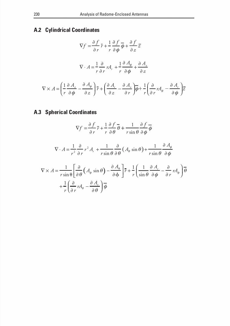
8/20/2019 Analysis of Radome-Enclosed Antennas
http://slidepdf.com/reader/full/analysis-of-radome-enclosed-antennas 251/319
A.2 Cylindrical Coordinates
∇ = + + f f
r
r
r
f f
z
z ∂
∂
∂
∂ φ
φ ∂
∂
1
∇ ⋅ = + + A r r
rA r
A A
z r
z 1 1∂
∂
∂
∂ φ
∂
∂
φ
∇ × = −
+ −
A r
A A
z r
A
z
A
r r r r z r z 1 1∂
∂ φ
∂
∂
∂
∂
∂
∂ φ
∂
∂
φ A
A z r
φ
∂
∂ φ
A.3 Spherical Coordinates
∇ = + f f
r r
r
f
r
f ∂
∂
∂
∂ θθ +
θ
∂
∂ φ φ
1 1
sin
( )∇ ⋅ = + + A
r r
r A
r
A
r
A r
1 1 12
2∂
∂ θ
∂
∂ θ
θ
θ
∂
∂ φθ
φ
sin
sin
sin
( )∇ × = −
+ − A
r A
A r
r
A
r r r 1 1 1
sinsin
sin
∂
∂ θθ
∂
∂ θ
∂
∂ φ
∂
∂ φ A
r r rA
A r
φ
θ
θ
∂
∂
∂
∂ θ φ
+ −
1
230 Analysis of Radome-Enclosed Antennas

8/20/2019 Analysis of Radome-Enclosed Antennas
http://slidepdf.com/reader/full/analysis-of-radome-enclosed-antennas 252/319
Appendix BPropagation Constant and WaveImpedance for Arbitrary Media
In Chapter 5 we presented a boundary value problem based matrix solution forcomputing the electromagnetic wave transmission and insertion phase delay fora signal propagating through a multilayer dielectric radome wall. That analysisaccounted for the dielectric losses in each of the dielectric layers via a loss tan-gent term associated with the layer. In this appendix, we consider a dielectricmaterial that has both a loss tangent term and a conductivity term, and the elec-tromagnetic wave behavior in such materials. As a result of the mathematicaldevelopment, the reader should be able to determine the propagation constant,apparent permittivity, and wave impedance.
The assumptions made in the mathematical development that followsapply to most candidate radome materials:
• The material is nonmagnetic, therefore µ = µo ;
• The conductivity term is totally real, that is, σ = σ ′;• The dielectric term is both real and imaginary, and can be modeled
via ε = ε′ − j ε″ .
B.1 Wave Components in Media
We start with the time-domain form of Maxwell’s curl equations:
231

8/20/2019 Analysis of Radome-Enclosed Antennas
http://slidepdf.com/reader/full/analysis-of-radome-enclosed-antennas 253/319
∇ × = −E H
t o µ ∂
∂(B.1)
∇ × = +H E E t
σ ε ∂∂
(B.2)
The general curl of a vector A in rectangular coordinates is:
∇
A
A
y
A
z x
A
z
A
x y
Ay
x
A z y x z ∂
∂
∂
∂
∂
∂
∂
∂
∂
∂
∂ x
y z
∂
(B.3)
In the following development, we will also assume that we have a trans-verse electromagnetic (TEM) wave traveling in the positive z direction that hasonly E x and H y components. (For normal incidence on a dielectric surface, thereader can derive an identical result by considering a wave that has only E y andH x components.) Accordingly, we can write
∇ × = −E E
z y
E
y z x x ∂
∂
∂
∂(B.4)
∇ H H
z x
H
x z
y y 2∂
∂
∂
∂(B.5)
If the function is both y and x invariant, then these two expressions reduceto:
∇ × = = −E E
z y
H
t y x o
y ∂
∂ µ
∂
∂ (B.6)
or
∂
∂ µ
∂
∂
E
z
H
t x
o
y = − (B.7)
Similarly,
∇ × = − = +H H
z x E x
E
t x
y
x x
∂
∂ σ ε
∂
∂(B.8)
232 Analysis of Radome-Enclosed Antennas
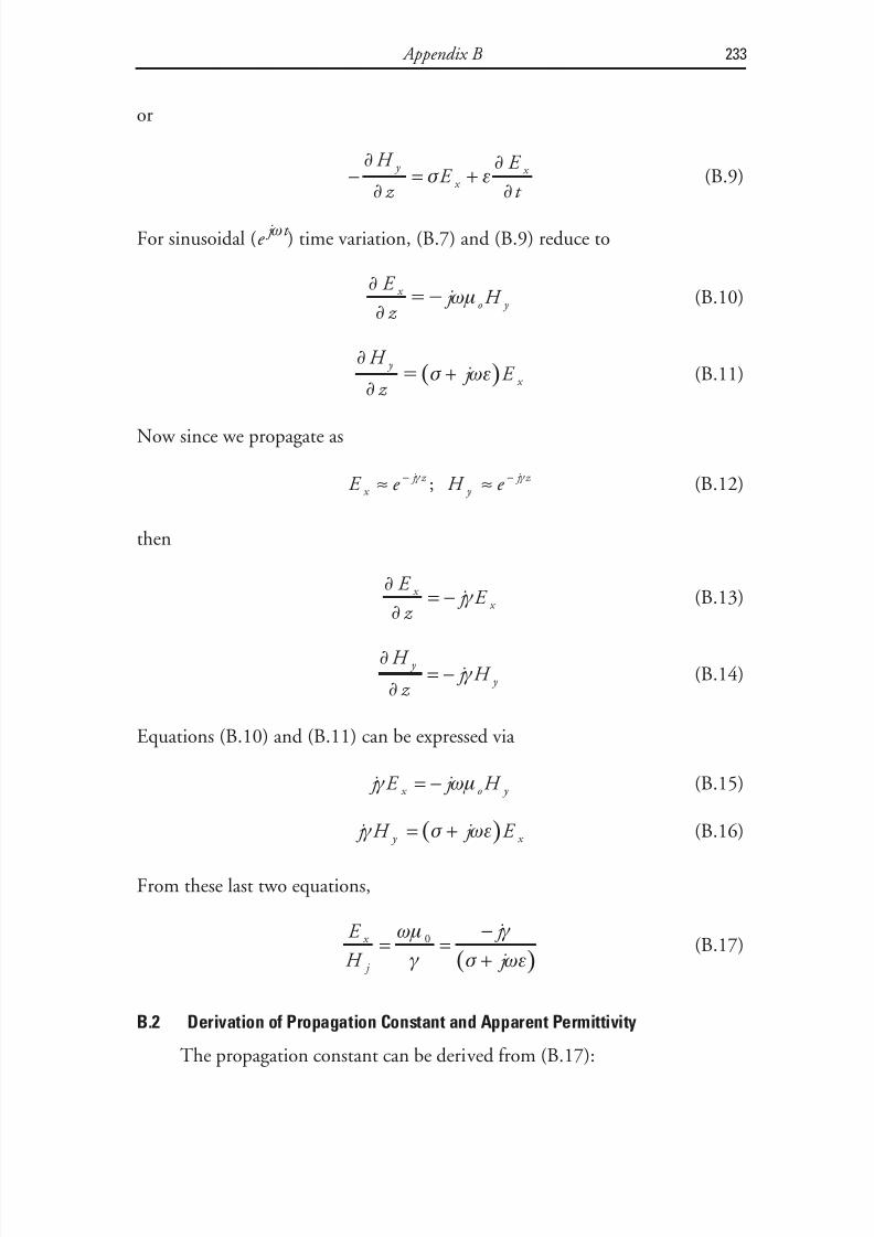
8/20/2019 Analysis of Radome-Enclosed Antennas
http://slidepdf.com/reader/full/analysis-of-radome-enclosed-antennas 254/319

8/20/2019 Analysis of Radome-Enclosed Antennas
http://slidepdf.com/reader/full/analysis-of-radome-enclosed-antennas 255/319
γ ω µε ωµ σ 2 2= − j o (B.18)
Or, in terms of the real and imaginary parts of the permittivity:
γ ω ω ε ω µ ε ωµ σ ω µ ε ε
ε
σ
ωε2 2 2 2 1= ′ − ′′ − = ′ −
′′′ +
′
o o o o j j j
(B.19)
From this last equation, together with the definition of loss tangent, weobtain the result:
γ ω µ ε δ
σ
ωε δ
σ
ωε= ′ − + ′
= − + ′
2
1 1o j k j tan tan (B.20)
Comparing this to the expression in Chapter 5 for a material without a conductivity term, we obtain the following for a complex apparent permittivity:
ε ε δ σ
ωε= ′ − +
′
1 j tan (B.21)
Or, the relative apparent permittivity is
ε ε δ σ
ωε εr r
o r
j = ′ − +′
1 tan (B.22)
B.3 Wave Impedance
From (B.20), we can obtain
γ δ σ
ωε
δ σ
ω= + +′
− +′
−
k e j
12 0 25
0 5 1
tan
.. tan tan
ε
(B.23)
If we incorporate this into (B.17) and express the result in terms of the rel-ative apparent permittivity, we obtain the wave impedance for normalincidence:
234 Analysis of Radome-Enclosed Antennas

8/20/2019 Analysis of Radome-Enclosed Antennas
http://slidepdf.com/reader/full/analysis-of-radome-enclosed-antennas 256/319
Z
e j
o r
o r
= ′
+ + ′
− +′
120
1
0 5 1 π
ε
δ σ
ωε ε
δ σ
ωε ε. tan tan
tan
(B.24)
This can be used to calculate the interfacial Fresnel reflection and trans-mission coefficients.
For other than normal incidence, assume the wave is propagating fromone medium to a second medium. The impedance just inside the interfacialboundary in the direction of propagation is modified for perpendicular and par-
allel polarization via the following approximations. For perpendicularpolarization:
Z
r
⊥ =−
1202
π θ
ε θ
cos
sin(B.25)
and for parallel polarization:
Z r
r
= −120 2 π ε θε θ
sin
cos(B.26)
where θ is the angle of incidence with respect to the surface normal, and thereader should use the apparent relative permittivity given by (B.22).
Appendix B 235

8/20/2019 Analysis of Radome-Enclosed Antennas
http://slidepdf.com/reader/full/analysis-of-radome-enclosed-antennas 257/319

8/20/2019 Analysis of Radome-Enclosed Antennas
http://slidepdf.com/reader/full/analysis-of-radome-enclosed-antennas 258/319
Appendix CMultilayer Propagation and FresnelTransmission and Reflection Coefficients
This appendix deals with the matrix solution for computing the transmitted andreflected electromagnetic wave components for a multilayer dielectric wall. Spe-cifically, for the single-layer wall depicted in Figure C.1, the reflected and trans-mitted wave components may be computed from the following matrix solution:
E
E T
R
R
e
e
jk t
jk t
0
0 1
1
1
1 1
1
0
0
11 1
1 1
+
− −
=
T
R
R
E
2
2
2
21
1 0
+
(C.1)
from which
E E T
e R e R e e
jk t jk t
jk t jk t 0
0 1
1
1
1 1 1 1 1
1 1 1 1
+
−
−
+ −
=
+
1 11 02
2
2
2
T R
R E (C.2)
In these equations, T 1 and T 2 are the front face and rear face voltage Fres-nel transmission coefficients, respectively, and R 1 and R 2 are the front face andrear face voltage Fresnel reflection coefficients, respectively. The parameter k 1 isthe wavenumber within dielectric material while t 1 is the thickness of the mate-rial. It is recommended that the thickness be calculated in centimeters and the
wave number be calculated in units of cm−1.For a two-layer wall depicted in Figure C.2, the reflected and transmitted
wave components may be computed from the following matrix solution:
237

8/20/2019 Analysis of Radome-Enclosed Antennas
http://slidepdf.com/reader/full/analysis-of-radome-enclosed-antennas 259/319
E
E T
R
R
e
e
jk t
jk t
0
0 1
1
1
1 1
1
0
0
1
1 1
1 1
+
− −
=
T
R
R
e
e T
R
R
jk t
jk t 2
2
2 3
3
3
1
1
0
0
1 1
1
2 2
2 2
−
E 30
+
(C.3)
from which
E
E T
e R e
R e e
jk t jk t
jk t jk t
0
0 1
1
1
1 1 1 1 1
1 1 1 1
+
−
−
+ −
=
−
+ −
1 1
12
2
2
1
1
2 2 2 2
2 2 2 2T
R
R
e R e
R e e
jk t jk t
jk t jk t
+1 1
1 03
3
3
3
T
R
R
E
(C.4)
where T i , R i , t i , and k i are the voltage Fresnel transmission coefficient, voltageFresnel reflection coefficient, thickness, and wave number for the i th layer,respectively, as implied in the single-layer case.
Lastly, we can generalize the result for the N -layer dielectric wall depictedin Figure C.3.
238 Analysis of Radome-Enclosed Antennas
E0
+
E0
−E
1
+
E1
+E2
+
E2
+
Layer 1
k t ,1 1
Figure C.1 Matrix solution for a single-layer dielectric wall.
E0
+
E0
−E1
+
E1
+E
2
+
E2
+
Layer 1
k t ,1 1
E3
+
E3−
k t ,2 2
Layer 2
Figure C.2 Matrix solution for a two-layer dielectric wall.

8/20/2019 Analysis of Radome-Enclosed Antennas
http://slidepdf.com/reader/full/analysis-of-radome-enclosed-antennas 260/319
Specifically, the front face reflected and net transmitted wave componentsmay be computed via:
E
E T
R
R
e
e i i
N i
i
jk ti
jk t
i
i i
0
0 1
1 1
1
0
0
+
−=
−
=
∏
+
+
+
++
1 1
1 01
1
1
1
T
R
R
E
N
N
N
N
(C.5)
from which we obtain the final result:
E
E T
e R e
R e e i i
N jk t i
jk t
i jk t jk
i i i i
i i i
0
0 1
1+
−=
−
+ −
= ∏ t
N
N
N
N
i
T
R
R
E
+
+
+
++
1 1
1 01
1
1
1
(C.6)
where all the parameters in (C.5) and (C.6) follow the implications of the single-and two-layer cases discussed previously.
C.1 Fresnel Transmission and Reflection Coefficients
The calculation of these coefficients can be accomplished by a number of differ-ent methods and are all seen to be a function of the wave polarization, angle of incidence with respect to the surface normal, wavenumbers in the respectivematerials, and the refractive index of the material. One approximation is to
neglect the complex component of the refractive index (loss term) in which weobtain for the perpendicular polarization case:
R n n
n n i i t t
i i t t
= −
+cos cos
cos cos
θ θ
θ θ(C.7)
Appendix C 239
E0
+
E0
−E
1
−
E1
+E2
+
E2
−
Layer 1
k t ,1 1
EN +1
+
EN
+1
−
k t ,2 2
Layer 2
EN
+
EN
−
k t ,N N
Layer N
Figure C.3 Matrix solution for an N -layer dielectric wall.

8/20/2019 Analysis of Radome-Enclosed Antennas
http://slidepdf.com/reader/full/analysis-of-radome-enclosed-antennas 261/319
wheren
i , n t = the real part of the refractive indices on the left and right sides of
the interface, respectively;
θi , θt = the angles of incidence with respect to the surface normal on theleft side and right side of the interface, respectively, and are easily com-puted by Snell’s law.
Likewise, one expression for the voltage transmission coefficient for theperpendicular wave component is:
T n
n n i i
i i t t
=+
2 cos
cos cos
θ
θ θ(C.8)
For the parallel polarization wave components, these two equations reduceto:
R n n
n n i t t i
i t t i
= −
+cos cos
cos cos
θ θ
θ θ(C.9)
and
T n
n n i i
i t t i
=+
2 cos
cos cos
θ
θ θ(C.10)
A simplification of all these formulas may be applied; for the perpendicu-lar polarization we obtain:
( )( )R
t i
t i = −
+sin
sin
θ θ
θ θ (C.11)
and for the parallel wave component,
( )( )R t i
t i
= −
+tan
tan
θ θ
θ θ(C.12)
and the respective transmission coefficient corresponding to each of these by applying:
T R = −1 2 (C.13)
240 Analysis of Radome-Enclosed Antennas
8/20/2019 Analysis of Radome-Enclosed Antennas
http://slidepdf.com/reader/full/analysis-of-radome-enclosed-antennas 262/319
Appendix DRadiation from Elemental Currents
The purpose of this appendix is to derive expressions for both the electromag-netic field and the array factor for an ensemble of infinitesimal (dipole) currentelements. Three cases are considered as illustrated in Figure D.1:
1. Current elements that are z -directed;2. Current elements that are x -directed;
3. Current elements that are y -directed.
The far-field radiation pattern of an infinitesimal dipole element followsfrom solution of Maxwell’s equations. Assuming a time harmonic field that ise j t dependent, the fundamental relations are expressed as the curl and diver-gence operators:
∇ × = +H j E J ωε0 (D.1)
∇ × =E j H ωµ 0 (D.2)
where εo and µo are the permittivity and permeability of free space, B H = µ 0
and D E = ε0 .Now, define a magnetic vector potential via
H A = ∇ ×
241

8/20/2019 Analysis of Radome-Enclosed Antennas
http://slidepdf.com/reader/full/analysis-of-radome-enclosed-antennas 263/319
then from (D.2) and (D.3), we obtain
( )∇ × + =E j A ωµ 0 0
Because any curl-free vector can be defined as the gradient of a scalar func-tion, one can define an electric scalar potential Φ where
242 Analysis of Radome-Enclosed Antennas
(b)
(a)
Figure D.1 Radiation from infinitesimal currents: (a) z -directed, (b) x -directed, and (c)
y -directed.

8/20/2019 Analysis of Radome-Enclosed Antennas
http://slidepdf.com/reader/full/analysis-of-radome-enclosed-antennas 264/319
E j A + = −∇ ωµ 0 Φ (D.5)
From (D.1), (D.3), and (D.5), we obtain
( )∇ ∇ ⋅ − ∇ − = − ∇ + A A k A j J 2 20 ωε Φ (D.6)
A vector is uniquely specified by both the curl and divergence. If wechoose
( )∇ ∇ ⋅ = − ∇ A j ωε0 Φ (D.7)
∇ + = −2 2 A k A J (D.8)
we obtain the well-known Helmholtz wave equation. Solutions to the field com-ponents for A follow from (D.3), (D.5), and (D.7):
H A = ∇ × (D.9)
( )E j A j
A = − + ∇ ∇ ⋅ ωµ ωε
0
0
1(D.10)
Appendix D 243
(c)
Figure D.1 (continued)

8/20/2019 Analysis of Radome-Enclosed Antennas
http://slidepdf.com/reader/full/analysis-of-radome-enclosed-antennas 265/319
Because rectangular components of A only have corresponding compo-nents of J as their source, the technique is first developed by assuming only a z -directed current element at the origin of a standard spherical coordinate sys-
tem, as depicted in Figure D.1(a). We assume current of magnitude I o andlength d .
∇ − =2 2 A k A I d z z o (D.11)
where k is the free-space wave number, h is the infinitesimal dipole length, and I o
is the current magnitude. Assume A z is r dependent. The differential equation tobe solved is
12
2 2
r r r r
A
r k A I d z
z o ∂
∂
∂
∂
∂
+ = (D.12)
A I e
r z o
jkr
=−
4 π(D.13)
From (D.9)
H zA A
r r z z = ∇ × = ×
∂
∂(D.14)
from which we obtain (in the far field)
H jkI d e
r o
jkr
φ π
θ=−
4sin (D.15)
E jk I d jkr
r o θ η
πθ=
−4
sin (D.16)
where
η µ
ε π= =o
o
120 (D.17)
Equations (D.15) and (D.16) can be shown to be equivalent to
E j A z θ ωε θ= 0 sin (D.18)
244 Analysis of Radome-Enclosed Antennas

8/20/2019 Analysis of Radome-Enclosed Antennas
http://slidepdf.com/reader/full/analysis-of-radome-enclosed-antennas 266/319
H E φ θ η
= 1
(D.19)
The relationship between far-field patterns and aperture currents followsfrom linear superposition of the radiated fields from each of the infinitesimalcurrents. For example, consider the z -directed current distribution shown inFigure D.1(a). The location of currents in the x direction is
x md x = (D.20)
and the location of currents in the y direction is
y nd y = (D.21)
In these last two equations, m and n are integers, where m = 0, 1, 2, ..., M and n = 0, 1, 2, ..., N , and d x and d y are the current spacings in the x and y direc-tions, respectively. The total current is given by the formula
( ) ( ) ( )I I x md y nd z mn x y
n
N
m
M
= − −
==
∑∑ δ δ δ00
(D.22)
where the Dirac delta functions are defined by the following relations:
( )δ p p
p
0 0
1 0
;
;
for all ≠=
for
(D.23)
(D.24)
Using this discrete current distribution in (D.13), we obtain
( ) ( ) ( ) A e
r z I x md y nd dx dy dz z
jkr
mn x y n
N
m
M
= − −−
==∑∑∫ ∫ ∫ 4 00 π
δ δ δ (D.25)
For a fixed distance from the antenna, r o , this reduces to
( ) A
e
r Ilmn z
jkr e
n
N jk md x nd y
=
−
=
− +0
4 0 0 π
θ φ φsin cos sin
∑∑=m
M
0
(D.26)
This result is sufficient to obtain far-field radiation patterns. Specifically,the far-field pattern is a simple sum of the current contributions of the
Appendix D 245

8/20/2019 Analysis of Radome-Enclosed Antennas
http://slidepdf.com/reader/full/analysis-of-radome-enclosed-antennas 267/319

8/20/2019 Analysis of Radome-Enclosed Antennas
http://slidepdf.com/reader/full/analysis-of-radome-enclosed-antennas 268/319
Appendix EProgram TORADOME Software Listing
#COMPILE EXE
FUNCTION PBMAIN
‘———— RADOME SHAPE PARAMETERS ——————————————————————
GLOBAL x0, y0, z0, L0, D0, Adia, AZ, EL, FREQUENCY AS SINGLE
GLOBAL DRAD, Adia, INCREMENT, RADIUS, MAGAouter() AS SINGLE
GLOBAL PHASEAouter(), Ainner(), PI AS SINGLE
GLOBAL AZ, EL, EDB(),RE, IM, CNST, JACK AS SINGLE
‘———— VECTOR PARAMETERS —————————————————————————
GLOBAL BTO, RTO, Ix, x, y, z, xi, yi, zi, Nt, Nx, Ny, Nz, COUNTA
AS SINGLE
GLOBAL COUNTB, xp, yp, zp, RE, IM, PHI, alpha, ri, rp, MATTHEW AS
SINGLE
GLOBAL MARK, LUKE, JOHN, times, EY, EZ, VV(), CONV, theta AS
SINGLE
GLOBAL Kx, Ky, Kz, IZ, IY, IZZ, IYY, VH(), I, J, II, JJ, M, MM, MMM
AS SINGLE
GLOBAL DR(), GR(), DUMB, VV(), VH(), XAZ, XEL, NAT AS SINGLE
GLOBAL EPOL, REU, IMU, REL, IML AS SINGLE
DIM Ainner(-50 TO 50, -50 TO 50), MAGAouter(-50 TO 50, -50 TO 50)
DIM PHASEAouter(-50 TO 50,-50 TO 50)
DIM EDB(-90 TO 90,-90 TO 90), VV(3), VH(3), DR(3), GR(3)
‘———— GLOBAL VARIABLES NEEDED IN SUBROUTINE WALL ————————————-
GLOBAL wavenumber, ER(), LTAN(), THK(), gamma, Ttotmag() AS SINGLE
GLOBAL Ttotph(), Rtotmag(), Rtotph() AS SINGLE
GLOBAL N, K, THK(), XER(), XLTAN(), XIZ, XIY AS SINGLE
DIM ER(10), LTAN(10), THK(10), Ttotmag(2), Ttotph(2), Rtotmag(2),
Rtotph(2)
247

8/20/2019 Analysis of Radome-Enclosed Antennas
http://slidepdf.com/reader/full/analysis-of-radome-enclosed-antennas 269/319
‘———— USER INPUT VARIABLES ———————————————————————-
GLOBAL IO_FREQ, IO_LAYERS, IO_N, IO_N2, IO_ERRORTIMES AS SINGLE
GLOBAL IO_THK(), IO_ER(), IO_LTAN(), IO_cursor_y, IO_cursor_x AS
SINGLE
GLOBAL IO_varinput IO_StartFreq, IO_StopFreq AS SINGLE
GLOBAL IO_FILENAME, IO_keystroke, IO_vardump AS STRINGGLOBAL IO_RadomeDiameter, IO_RadomeLength AS SINGLE
GLOBAL IO_AntennaDiameter, IO_AntennaXo, IO_AntennaEL AS SINGLE
GLOBAL IO_AntennaAZ AS SINGLE
GLOBAL IO_AntennaPol AS STRING
DIM IO_THK(10), IO_ER(10), IO_LTAN(10)
‘———— ADDED TO MAKE RUN —————————————————————————
GLOBAL keystroke AS STRING
GLOBAL pol, BSE, NAT, XTHK(), XER(), XLTAN(), XAZ, XEL AS SINGLE
GLOBAL StartFreq, StopFreq, xPosRad AS SINGLE
DIM XTHK(10), XER(10), XLTAN(10)
‘———— CONSTANTS —————————————————————————————
DRAD=3.14159265/180
PI=3.14159265
‘*********************************************************************
‘* START Subroutine *
‘*********************************************************************
START:
COLOR 15,1
CLS
COLOR 15,14
LOCATE 1,1
PRINT SPACE$(80);
COLOR 0,14
LOCATE 1,21
PRINT “TANGENT OGIVE RADOME ANALYSIS DEMO PROGRAM”
COLOR 15,1LOCATE 10,1
PRINT “ This software computes the transmission loss through a
tangent ogive”
PRINT “ shaped radome. The radome wall can be a multilayer compos-
ite with up to”
PRINT “ five(5) layers of different material types and thick-
nesses.”
LOCATE 23,1
COLOR 9,1
PRINT “ www.Radomes.net ”
COLOR 9,7
248 Analysis of Radome-Enclosed Antennas

8/20/2019 Analysis of Radome-Enclosed Antennas
http://slidepdf.com/reader/full/analysis-of-radome-enclosed-antennas 270/319
LOCATE 25,1
PRINT SPACE$(80);
LOCATE 1,1
COLOR 1,7
LOCATE 25,28
PRINT “<Press Any Key> to Continue”;
CURSOR OFF
DO
IO_keystroke = INKEY$
IF IO_keystroke ><“” THEN EXIT DO
LOOP
‘*********************************************************************‘* IO_RESTART Subroutine - Radome Geometry *
‘*********************************************************************
IO_RESTART:
CURSOR OFF
COLOR 15,1
CLS
COLOR 15,14
LOCATE 1,1
PRINT SPACE$(80);
COLOR 0,14
LOCATE 1,28
PRINT “RADOME GEOMETRY DESCRIPTION”
COLOR 1,7
LOCATE 25,1
PRINT SPACE$(80);
LOCATE 1,1
COLOR 8,1
LOCATE 22,4
PRINT “<Arrow Keys>-Move Cursor <Enter>-Edit Data <F1>-Next Page
<Esc>-Exit”;
COLOR 15,1
COLOR 9,7
LOCATE 24,1
PRINT SPACE$(80);
LOCATE 25,1
PRINT SPACE$(80);LOCATE 1,1
COLOR 1,7
LOCATE 24,2
PRINT “NOTE: To Change Data, Use Arrow Keys to Select Desired
Appendix E 249

8/20/2019 Analysis of Radome-Enclosed Antennas
http://slidepdf.com/reader/full/analysis-of-radome-enclosed-antennas 271/319
Field, Then Press the”;
LOCATE 25,8
PRINT “Enter Key to Edit Data Within That Field. Press Enter Again
When Done.”;
COLOR 15,1
ON ERROR GOTO IO_PROGRAMERROR1
IF IO_ERRORTIMES >= 3 THEN
COLOR 15,0
BEEP
PRINT “ UNRECOVERABLE ERROR IN PROGRAM EXECUTION!
SLEEP 7000
END
END IF
OPEN “C:\RADGEO.DAT” FOR INPUT AS #1
‘—— CURSOR ——
INPUT #1, IO_cursor_y
INPUT #1, IO_cursor_x
‘—— DATA ——
INPUT #1, IO_StartFreq
INPUT #1, IO_StopFreq
INPUT #1, IO_RadomeDiameter
INPUT #1, IO_RadomeLength
INPUT #1, IO_AntennaDiameter
INPUT #1, IO_AntennaEL
INPUT #1, IO_AntennaAZ
INPUT #1, IO_AntennaXo
INPUT #1, IO_AntennaPol
CLOSE #1
COLOR 15,1
LOCATE 3,2
PRINT “Start Frequency(GHz) = ”;
COLOR 15,0
IO_vardump = USING$ (“ ###.## ”, IO_StartFreq)
PRINT IO_vardump
COLOR 15,1
LOCATE 5,2
PRINT “Stop Frequency(GHz) = ”;
COLOR 15,0
IO_vardump = USING$ (“ ###.## ”, IO_StopFreq)
PRINT IO_vardump
COLOR 15,1
LOCATE 7,2PRINT “Radome Diameter = ”;
COLOR 15,0
IO_vardump = USING$ (“ ###.## ”, IO_RadomeDiameter)
PRINT IO_vardump
COLOR 15,1
250 Analysis of Radome-Enclosed Antennas

8/20/2019 Analysis of Radome-Enclosed Antennas
http://slidepdf.com/reader/full/analysis-of-radome-enclosed-antennas 272/319
LOCATE 9,2
PRINT “Radome Length = ”;
COLOR 15,0
IO_vardump = USING$ (“ ###.## ”, IO_RadomeLength)
PRINT IO_vardump
COLOR 15,1
LOCATE 11,2
PRINT “Antenna Diameter = ”;
COLOR 15,0
IO_vardump = USING$ (“ ###.## ”, IO_AntennaDiameter)
PRINT IO_vardump
COLOR 15,1
LOCATE 13,2
PRINT “Elevation(deg) = ”;
COLOR 15,0
IO_vardump = USING$ (“ ###.## ”, IO_AntennaEL)
PRINT IO_vardump
COLOR 15,1
LOCATE 15,2
PRINT “Azimuth(deg) = ”;
COLOR 15,0
IO_vardump = USING$ (“ ###.## ”, IO_AntennaAZ)
PRINT IO_vardump
COLOR 15,1
LOCATE 17,2
PRINT “Antenna Xo Location = ”;
COLOR 15,0
IO_vardump = USING$ (“ ###.## ”, IO_AntennaXo)
PRINT IO_vardump
COLOR 15,1
LOCATE 19,2
PRINT “Antenna Polarization = ”;
COLOR 15,0IO_vardump = USING$ (“ & ”, IO_AntennaPol)
PRINT IO_vardump
COLOR 15,1
CURSOR OFF
LOCATE IO_cursor_y, IO_cursor_x
PRINT CHR$(16);
DO
IO_keystroke = INKEY$
IF IO_keystroke = CHR$(27) THEN END
IF IO_keystroke = CHR$(0) + CHR$(72) THEN
IF IO_cursor_y > 4 THEN
Appendix E 251
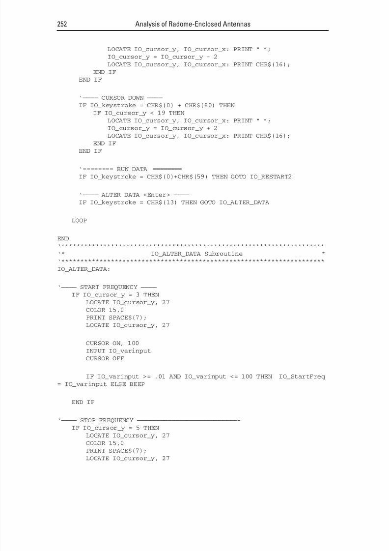
8/20/2019 Analysis of Radome-Enclosed Antennas
http://slidepdf.com/reader/full/analysis-of-radome-enclosed-antennas 273/319

8/20/2019 Analysis of Radome-Enclosed Antennas
http://slidepdf.com/reader/full/analysis-of-radome-enclosed-antennas 274/319
CURSOR ON, 100
INPUT IO_varinput
CURSOR OFF
IF IO_varinput >= .01 AND IO_varinput <= 100 THEN IO_StopFreq
= IO_varinput ELSE BEEP
END IF
‘———— RADOME DIAMETER ——————————————————————————
IF IO_cursor_y = 7 THEN
LOCATE IO_cursor_y, 27
COLOR 15,0
PRINT SPACE$(7);
LOCATE IO_cursor_y, 27
CURSOR ON, 100
INPUT IO_varinput
CURSOR OFF
IF IO_varinput < 999.99 AND IO_varinput >= 1 THEN
IO_RadomeDiameter = IO_varinput ELSE BEEP
END IF
‘———— RADOME LENGTH ———————————————————————————IF IO_cursor_y = 9 THEN
LOCATE IO_cursor_y, 27
COLOR 15,0
PRINT SPACE$(7);
LOCATE IO_cursor_y, 27
CURSOR ON, 100
INPUT IO_varinput
CURSOR OFF
IF IO_varinput < 999.99 AND IO_varinput >= 1 THEN
IO_RadomeLength = IO_varinput ELSE BEEP
END IF
‘———— ANTENNA DIAMETER —————————————————————————-
IF IO_cursor_y = 11 THEN
LOCATE IO_cursor_y, 27
COLOR 15,0
PRINT SPACE$(7);
LOCATE IO_cursor_y, 27
CURSOR ON, 100
INPUT IO_varinput
CURSOR OFF
Appendix E 253

8/20/2019 Analysis of Radome-Enclosed Antennas
http://slidepdf.com/reader/full/analysis-of-radome-enclosed-antennas 275/319
IF IO_varinput < 999.99 AND IO_varinput >= 1 THEN
IO_AntennaDiameter = IO_varinput ELSE BEEP
END IF
‘———— ELEVATION —————————————————————————————
IF IO_cursor_y = 13 THEN
LOCATE IO_cursor_y, 27
COLOR 15,0
PRINT SPACE$(7);
LOCATE IO_cursor_y, 27
CURSOR ON, 100
INPUT IO_varinput
CURSOR OFF
IF IO_varinput >= 0 AND IO_varinput <= 90 THEN IO_AntennaEL =
IO_varinput ELSE BEEP
END IF
‘———— AZIMUTH ——————————————————————————————
IF IO_cursor_y = 15 THEN
LOCATE IO_cursor_y, 27
COLOR 15,0
PRINT SPACE$(7);
LOCATE IO_cursor_y, 27
CURSOR ON, 100
INPUT IO_varinput
CURSOR OFF
IF IO_varinput >=0 AND IO_varinput <=90 THEN IO_AntennaAZ =
IO_varinput ELSE BEEP
END IF
‘———— ANTENNA Xo LOCATION ————————————————————————
IF IO_cursor_y = 17 THEN
LOCATE IO_cursor_y, 27
COLOR 15,0
PRINT SPACE$(7);
LOCATE IO_cursor_y, 27
CURSOR ON, 100
INPUT IO_varinput
CURSOR OFF
IF IO_varinput >= 0 AND IO_varinput <= 999.99 THEN
IO_AntennaXo = IO_varinput ELSE BEEP
END IF
254 Analysis of Radome-Enclosed Antennas

8/20/2019 Analysis of Radome-Enclosed Antennas
http://slidepdf.com/reader/full/analysis-of-radome-enclosed-antennas 276/319
‘———— ANTENNA POLARIZATION ———————————————————————-
IF IO_cursor_y = 19 THEN
LOCATE IO_cursor_y, 27
COLOR 15,0
PRINT SPACE$(9);
LOCATE IO_cursor_y, 27
IF IO_AntennaPol = “Vertical” THEN
IO_AntennaPol = “Horizonal”
ELSE
IO_AntennaPol = “Vertical”
END IF
END IF
CLOSEOPEN “C:\RADGEO.DAT” FOR OUTPUT AS #1
‘—— CURSOR ——
PRINT #1, IO_cursor_y
PRINT #1, IO_cursor_x
‘—— DATA ——
PRINT #1, IO_StartFreq
PRINT #1, IO_StopFreq
PRINT #1, IO_RadomeDiameter
PRINT #1, IO_RadomeLength
PRINT #1, IO_AntennaDiameter
PRINT #1, IO_AntennaEL
PRINT #1, IO_AntennaAZ
PRINT #1, IO_AntennaXo
PRINT #1, IO_AntennaPol
CLOSE #1
GOTO IO_restart
‘*********************************************************************
‘* IO_RESTART2 Subroutine *
‘*********************************************************************
IO_RESTART2:
‘———— TEST FOR ANTENNA HITTING WALL ———————————————————
BTO=(4*IO_RadomeLength^2-IO_RadomeDiameter^2)/(4*IO_RadomeDiameter)
RTO=(4*IO_RadomeLength^2+IO_RadomeDiameter^2)/(4*IO_RadomeDiameter)
xPosRad = (SQR(RTO^2) - IO_AntennaXo^2) - BTO
IF (IO_AntennaDiameter + .5) > (2 * xPosRad) THEN
BEEP
COLOR 15,12
LOCATE 22,1
PRINT SPACE$(80);
Appendix E 255

8/20/2019 Analysis of Radome-Enclosed Antennas
http://slidepdf.com/reader/full/analysis-of-radome-enclosed-antennas 277/319
LOCATE 22,2
PRINT “ANTENNA EDGE HITS RADOME WALL, ALTER ANTENNA SIZE,
RADOME SIZE OR Xo-LOCATION”
GOSUB waitforanykey
GOTO IO_RESTART
END IF
‘———— TEST FOR LESS THAN HEMISPHERE ———————————————————
IF IO_RadomeLength < (IO_RadomeDiameter/2) THEN
BEEP
COLOR 15,12
LOCATE 22,1
PRINT SPACE$(80);
LOCATE 22,2
PRINT “RADOME DIMENSIONS ARE LESS THAN A HEMISPHERE, ALTER
RADOME LENGTH OR DIAMETER”
GOSUB waitforanykey
GOTO IO_RESTART
END IF
COLOR 15,1
CLS
COLOR 15,14
LOCATE 1,1
PRINT SPACE$(80);
COLOR 0,14
LOCATE 1,30
PRINT “WALL LAYER DESCRIPTION”
COLOR 8,1
LOCATE 22,4
PRINT “<Arrow Keys>-Move Cursor <Enter>-Edit Data <F1>-Run Data
<Esc>-Exit”;
COLOR 15,1
COLOR 9,7
LOCATE 24,1
PRINT SPACE$(80);
LOCATE 25,1
PRINT SPACE$(80);
LOCATE 1,1
COLOR 1,7
LOCATE 24,2
PRINT “NOTE: To Change Data, Use Arrow Keys to Select Desired
Field, Then Press the”;
LOCATE 25,8
256 Analysis of Radome-Enclosed Antennas

8/20/2019 Analysis of Radome-Enclosed Antennas
http://slidepdf.com/reader/full/analysis-of-radome-enclosed-antennas 278/319
PRINT “Enter Key to Edit Data Within That Field. Press Enter Again
When Done.”;
COLOR 15,1
ON ERROR GOTO IO_PROGRAMERROR2
IF IO_ERRORTIMES >= 3 THEN
COLOR 15,0
BEEP
PRINT “ UNRECOVERABLE ERROR IN PROGRAM EXECUTION!
SLEEP 7000
END
END IF
OPEN “C:\WALLDSC.DAT” FOR INPUT AS #1
‘—— CURSOR —
INPUT #1, IO_cursor_y
INPUT #1, IO_cursor_x
‘—— LAYERS ——
INPUT #1, IO_LAYERS
‘—— THK, ER, LTAN ——
FOR IO_N = 1 TO 5
INPUT #1, IO_THK(IO_N), IO_ER(IO_N), IO_LTAN(IO_N)
NEXT IO_N
CLOSE #1
LOCATE 3,2
PRINT “Number of Layers: ”;
COLOR 15,0
IO_vardump = USING$ (“ # ”, IO_LAYERS)
PRINT IO_vardump
COLOR 15,1
‘———— DIMLY PRINT ALL LAYERS ——————————————————————-
IO_N=0
FOR IO_N2 = 1 TO 10 STEP 2
IO_N = IO_N + 1
COLOR 0,1
LOCATE 4 + IO_N2,2
PRINT “Thickness(”;LTRIM$(STR$(IO_N));"): “;
IO_vardump = USING$ (“ #.### ”, IO_THK(IO_N))
PRINT IO_vardump
LOCATE 4 + IO_N2, 27
PRINT “Dielectric(”;LTRIM$(STR$(IO_N));"): “;
IO_vardump = USING$ (“ *0.## ”, IO_ER(IO_N))
PRINT IO_vardump
Appendix E 257

8/20/2019 Analysis of Radome-Enclosed Antennas
http://slidepdf.com/reader/full/analysis-of-radome-enclosed-antennas 279/319
LOCATE 4 + IO_N2, 53
PRINT “Loss Tangent(”;LTRIM$(STR$(IO_N));"): “;
IO_vardump = USING$ (“ #.#### ”, IO_LTAN(IO_N))
PRINT IO_vardump
NEXT IO_N2
‘———— HIGHLIGHT SELECTED NUMBER OF LAYERS ————————————————
IO_N = 0
FOR IO_N2 = 1 TO IO_LAYERS * 2 STEP 2
IO_N = IO_N+1
COLOR 15,1
LOCATE 4 + IO_N2,2
PRINT “Thickness(”;LTRIM$(STR$(IO_N));"): “;
COLOR 15,0
IO_vardump = USING$ (“ #.### ”, IO_THK(IO_N))
PRINT IO_vardump
COLOR 15,1
LOCATE 4 + IO_N2, 27
PRINT “Dielectric(”;LTRIM$(STR$(IO_N));"): “;
COLOR 15,0
IO_vardump = USING$ (“ *0.## ”, IO_ER(IO_N))
PRINT IO_vardump
COLOR 15,1
LOCATE 4 + IO_N2, 53
PRINT “Loss Tangent(”;LTRIM$(STR$(IO_N));"): “;
COLOR 15,0
IO_vardump = USING$ (“ #.#### ”, IO_LTAN(IO_N))
PRINT IO_vardump
COLOR 15,1
NEXT IO_N2
CURSOR OFF
LOCATE IO_cursor_y, IO_cursor_x
PRINT CHR$(16);
DO
IO_keystroke = INKEY$
IF IO_keystroke = CHR$(27) THEN GOTO IO_RESTART
258 Analysis of Radome-Enclosed Antennas
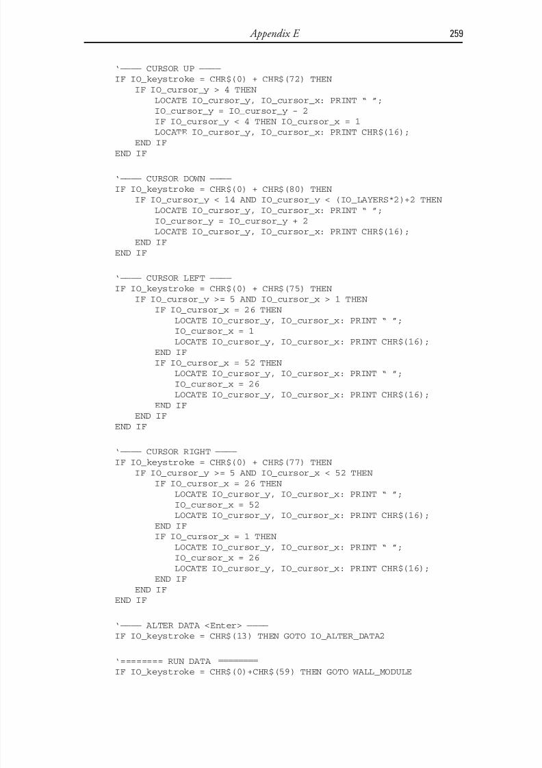
8/20/2019 Analysis of Radome-Enclosed Antennas
http://slidepdf.com/reader/full/analysis-of-radome-enclosed-antennas 280/319
‘———— CURSOR UP ————
IF IO_keystroke = CHR$(0) + CHR$(72) THEN
IF IO_cursor_y > 4 THEN
LOCATE IO_cursor_y, IO_cursor_x: PRINT “ ”;
IO_cursor_y = IO_cursor_y - 2
IF IO_cursor_y < 4 THEN IO_cursor_x = 1LOCATE IO_cursor_y, IO_cursor_x: PRINT CHR$(16);
END IF
END IF
‘———— CURSOR DOWN ————
IF IO_keystroke = CHR$(0) + CHR$(80) THEN
IF IO_cursor_y < 14 AND IO_cursor_y < (IO_LAYERS*2)+2 THEN
LOCATE IO_cursor_y, IO_cursor_x: PRINT “ ”;
IO_cursor_y = IO_cursor_y + 2
LOCATE IO_cursor_y, IO_cursor_x: PRINT CHR$(16);
END IFEND IF
‘———— CURSOR LEFT ————
IF IO_keystroke = CHR$(0) + CHR$(75) THEN
IF IO_cursor_y >= 5 AND IO_cursor_x > 1 THEN
IF IO_cursor_x = 26 THEN
LOCATE IO_cursor_y, IO_cursor_x: PRINT “ ”;
IO_cursor_x = 1
LOCATE IO_cursor_y, IO_cursor_x: PRINT CHR$(16);
END IF
IF IO_cursor_x = 52 THENLOCATE IO_cursor_y, IO_cursor_x: PRINT “ ”;
IO_cursor_x = 26
LOCATE IO_cursor_y, IO_cursor_x: PRINT CHR$(16);
END IF
END IF
END IF
‘———— CURSOR RIGHT ————
IF IO_keystroke = CHR$(0) + CHR$(77) THEN
IF IO_cursor_y >= 5 AND IO_cursor_x < 52 THEN
IF IO_cursor_x = 26 THENLOCATE IO_cursor_y, IO_cursor_x: PRINT “ ”;
IO_cursor_x = 52
LOCATE IO_cursor_y, IO_cursor_x: PRINT CHR$(16);
END IF
IF IO_cursor_x = 1 THEN
LOCATE IO_cursor_y, IO_cursor_x: PRINT “ ”;
IO_cursor_x = 26
LOCATE IO_cursor_y, IO_cursor_x: PRINT CHR$(16);
END IF
END IF
END IF
‘———— ALTER DATA <Enter> ————
IF IO_keystroke = CHR$(13) THEN GOTO IO_ALTER_DATA2
‘======== RUN DATA ========
IF IO_keystroke = CHR$(0)+CHR$(59) THEN GOTO WALL_MODULE
Appendix E 259
8/20/2019 Analysis of Radome-Enclosed Antennas
http://slidepdf.com/reader/full/analysis-of-radome-enclosed-antennas 281/319
LOOP
END
‘*********************************************************************IO_ALTER_DATA2:
‘———— LAYERS ——————————————————————————————-
IF IO_cursor_y = 3 AND IO_cursor_x = 1 THEN
LOCATE IO_cursor_y, 20
COLOR 15,0
PRINT SPACE$(3);
LOCATE IO_cursor_y, 21
CURSOR ON, 100
INPUT IO_varinputCURSOR OFF
IF IO_varinput => 1 AND IO_varinput <= 5 THEN IO_LAYERS =
INT(IO_varinput) ELSE BEEP
END IF
‘———— THICKNESS 1 ————————————————————————————
IF IO_cursor_y = 5 AND IO_cursor_x = 1 THENLOCATE IO_cursor_y, 17
COLOR 15,0
PRINT SPACE$(5);
LOCATE IO_cursor_y, 17
CURSOR ON, 100
INPUT IO_varinput
CURSOR OFF
IF IO_varinput => 0 AND IO_varinput <= 3 THEN IO_THK(1) =
IO_varinput ELSE BEEP
END IF
‘———— THICKNESS 2 ————————————————————————————
IF IO_cursor_y = 7 AND IO_cursor_x = 1 THEN
LOCATE IO_cursor_y, 17
COLOR 15,0
PRINT SPACE$(5);
LOCATE IO_cursor_y, 17
CURSOR ON, 100
INPUT IO_varinput
CURSOR OFF
IF IO_varinput => 0 AND IO_varinput <= 3 THEN IO_THK(2) =
IO_varinput ELSE BEEP
260 Analysis of Radome-Enclosed Antennas
8/20/2019 Analysis of Radome-Enclosed Antennas
http://slidepdf.com/reader/full/analysis-of-radome-enclosed-antennas 282/319
END IF
‘———— THICKNESS 3 ————————————————————————————
IF IO_cursor_y = 9 AND IO_cursor_x = 1 THEN
LOCATE IO_cursor_y, 17
COLOR 15,0
PRINT SPACE$(5);
LOCATE IO_cursor_y, 17
CURSOR ON, 100
INPUT IO_varinput
CURSOR OFF
IF IO_varinput => 0 AND IO_varinput <= 3 THEN IO_THK(3) =
IO_varinput ELSE BEEP
END IF
‘———— THICKNESS 4 ————————————————————————————
IF IO_cursor_y = 11 AND IO_cursor_x = 1 THEN
LOCATE IO_cursor_y, 17
COLOR 15,0
PRINT SPACE$(5);
LOCATE IO_cursor_y, 17
CURSOR ON, 100
INPUT IO_varinput
CURSOR OFF
IF IO_varinput => 0 AND IO_varinput <= 3 THEN IO_THK(4) =
IO_varinput ELSE BEEP
END IF
‘———— THICKNESS 5 ————————————————————————————
IF IO_cursor_y = 13 AND IO_cursor_x = 1 THEN
LOCATE IO_cursor_y, 17
COLOR 15,0
PRINT SPACE$(5);
LOCATE IO_cursor_y, 17
CURSOR ON, 100
INPUT IO_varinput
CURSOR OFF
IF IO_varinput => 0 AND IO_varinput <= 3 THEN IO_THK(5) =
IO_varinput ELSE BEEP
END IF
‘———— DIELECTRIC 1 ———————————————————————————-
IF IO_cursor_y = 5 AND IO_cursor_x = 26 THEN
LOCATE IO_cursor_y, 43
Appendix E 261

8/20/2019 Analysis of Radome-Enclosed Antennas
http://slidepdf.com/reader/full/analysis-of-radome-enclosed-antennas 283/319
COLOR 15,0
PRINT SPACE$(5);
LOCATE IO_cursor_y, 43
CURSOR ON, 100
INPUT IO_varinput
CURSOR OFF
IF IO_varinput => .01 AND IO_varinput <= 99 THEN IO_ER(1) =
IO_varinput ELSE BEEP
END IF
‘———— DIELECTRIC 2 ———————————————————————————-
IF IO_cursor_y = 7 AND IO_cursor_x = 26 THEN
LOCATE IO_cursor_y, 43COLOR 15,0
PRINT SPACE$(5);
LOCATE IO_cursor_y, 43
CURSOR ON, 100
INPUT IO_varinput
CURSOR OFF
IF IO_varinput => .01 AND IO_varinput <= 99 THEN IO_ER(2) =
IO_varinput ELSE BEEP
END IF
‘———— DIELECTRIC 3 ———————————————————————————-
IF IO_cursor_y = 9 AND IO_cursor_x = 26 THEN
LOCATE IO_cursor_y, 43
COLOR 15,0
PRINT SPACE$(5);
LOCATE IO_cursor_y, 43
CURSOR ON, 100
INPUT IO_varinput
CURSOR OFF
IF IO_varinput => .01 AND IO_varinput <= 99 THEN IO_ER(3) =
IO_varinput ELSE BEEP
END IF
‘———— DIELECTRIC 4 ———————————————————————————-
IF IO_cursor_y = 11 AND IO_cursor_x = 26 THENLOCATE IO_cursor_y, 43
COLOR 15,0
PRINT SPACE$(5);
LOCATE IO_cursor_y, 43
262 Analysis of Radome-Enclosed Antennas
8/20/2019 Analysis of Radome-Enclosed Antennas
http://slidepdf.com/reader/full/analysis-of-radome-enclosed-antennas 284/319
CURSOR ON, 100
INPUT IO_varinput
CURSOR OFF
IF IO_varinput => .01 AND IO_varinput <= 99 THEN IO_ER(4) =
IO_varinput ELSE BEEP
END IF
‘———— DIELECTRIC 5 ———————————————————————————-
IF IO_cursor_y = 13 AND IO_cursor_x = 26 THEN
LOCATE IO_cursor_y, 43
COLOR 15,0
PRINT SPACE$(5);
LOCATE IO_cursor_y, 43
CURSOR ON, 100
INPUT IO_varinput
CURSOR OFF
IF IO_varinput => .01 AND IO_varinput <= 99 THEN IO_ER(5) =
IO_varinput ELSE BEEP
END IF
‘———— LOSS TANGENT 1 ——————————————————————————-IF IO_cursor_y = 5 AND IO_cursor_x = 52 THEN
LOCATE IO_cursor_y, 71
COLOR 15,0
PRINT SPACE$(6);
LOCATE IO_cursor_y, 71
CURSOR ON, 100
INPUT IO_varinput
CURSOR OFF
IF IO_varinput => .0001 AND IO_varinput < 1 THEN IO_LTAN(1) =
IO_varinput ELSE BEEP
END IF
‘———— LOSS TANGENT 2 ——————————————————————————-
IF IO_cursor_y = 7 AND IO_cursor_x = 52 THEN
LOCATE IO_cursor_y, 71
COLOR 15,0
PRINT SPACE$(6);
LOCATE IO_cursor_y, 71
CURSOR ON, 100
INPUT IO_varinput
CURSOR OFF
Appendix E 263
8/20/2019 Analysis of Radome-Enclosed Antennas
http://slidepdf.com/reader/full/analysis-of-radome-enclosed-antennas 285/319
IF IO_varinput => .0001 AND IO_varinput < 1 THEN IO_LTAN(2) =
IO_varinput ELSE BEEP
END IF
‘———— LOSS TANGENT 3 ——————————————————————————-
IF IO_cursor_y = 9 AND IO_cursor_x = 52 THEN
LOCATE IO_cursor_y, 71
COLOR 15,0
PRINT SPACE$(6);
LOCATE IO_cursor_y, 71
CURSOR ON, 100
INPUT IO_varinput
CURSOR OFF
IF IO_varinput => .0001 AND IO_varinput < 1 THEN IO_LTAN(3) =
IO_varinput ELSE BEEP
END IF
‘———— LOSS TANGENT 4 ——————————————————————————-
IF IO_cursor_y = 11 AND IO_cursor_x = 52 THEN
LOCATE IO_cursor_y, 71
COLOR 15,0
PRINT SPACE$(6);
LOCATE IO_cursor_y, 71
CURSOR ON, 100
INPUT IO_varinput
CURSOR OFF
IF IO_varinput => .0001 AND IO_varinput < 1 THEN IO_LTAN(4) =
IO_varinput ELSE BEEP
END IF
‘———— LOSS TANGENT 5 ——————————————————————————-
IF IO_cursor_y = 13 AND IO_cursor_x = 52 THEN
LOCATE IO_cursor_y, 71
COLOR 15,0
PRINT SPACE$(6);
LOCATE IO_cursor_y, 71
CURSOR ON, 100
INPUT IO_varinput
CURSOR OFF
IF IO_varinput => .0001 AND IO_varinput < 1 THEN IO_LTAN(5) =
IO_varinput ELSE BEEP
END IF
264 Analysis of Radome-Enclosed Antennas

8/20/2019 Analysis of Radome-Enclosed Antennas
http://slidepdf.com/reader/full/analysis-of-radome-enclosed-antennas 286/319
CLOSE
OPEN “C:\WALLDSC.DAT” FOR OUTPUT AS #1
‘—— CURSOR ——
PRINT #1, IO_cursor_y
PRINT #1, IO_cursor_x
‘—— LAYERS ——PRINT #1, IO_LAYERS
‘—— THK, ER, LTAN ——
FOR IO_N = 1 TO 5
PRINT #1, IO_THK(IO_N), IO_ER(IO_N), IO_LTAN(IO_N)
NEXT IO_N
CLOSE #1
GOTO IO_restart2
‘*********************************************************************
‘* IO_PROGRAMERROR1 Subroutine *
‘*********************************************************************
IO_PROGRAMERROR1:
IF ERR = 53 THEN
CLOSE
OPEN “C:\RADGEO.DAT” FOR OUTPUT AS #1
‘—— CURSOR ——
PRINT #1, “3"
PRINT #1, ”1"
‘—— START FREQ ——
PRINT #1, “2"
‘—— STOP FREQ ——
PRINT #1, ”8"
‘—— RAD DIA ——
PRINT #1, “12"
‘—— RAD LENGTH ——
PRINT #1, ”24"
‘—— ANT DIA ——
PRINT #1, “8"
‘—— EL ——
PRINT #1, ”0"
‘—— AZ ——
PRINT #1, “0"
‘—— ANT LOCATION X ——
PRINT #1, ”0"
‘—— ANT POL ——
PRINT #1, “Vertical”
CLOSE #1
GOTO IO_RESTARTELSE
BEEP
COLOR 15,9
PRINT “ ERROR IN PROGRAM EXECUTION! ”
SLEEP 5000
END IF
Appendix E 265
8/20/2019 Analysis of Radome-Enclosed Antennas
http://slidepdf.com/reader/full/analysis-of-radome-enclosed-antennas 287/319
END
‘*********************************************************************
‘* IO_PROGRAMERROR2 Subroutine *
‘*********************************************************************
IO_PROGRAMERROR2:
IF ERR = 53 THEN
CLOSE
OPEN “C:\WALLDSC.DAT” FOR OUTPUT AS #1
‘—— CURSOR ——
PRINT #1, “3"
PRINT #1, ”1"
‘—— LAYERS ——
PRINT #1, “3"
‘—— THK, ER, LTAN ——
FOR IO_N = 1 TO 5
PRINT #1, ”.05, 3, .001"
NEXT IO_N
CLOSE #1
GOTO IO_RESTART
ELSE
BEEP
COLOR 15,9
PRINT “ ERROR IN PROGRAM EXECUTION! ”SLEEP 5000
END IF
END
‘*********************************************************************
‘* WALL_MODULE Subroutine *
‘*********************************************************************
WALL_MODULE:
GLOBAL DRAD, PI, FREQUENCY, wavenumber, ER(), LTAN(), THK() AS
SINGLE
GLOBAL GAMMA, GAMMADEG, TRANSMAG(), TRANSPHS() AS SINGLE
GLOBAL FREQSTART, FREQSTOP, Rtotmag(), Rtotph(), times AS SINGLE
GLOBAL vardump, dummy AS STRING
COLOR 15,1
CLS
COLOR 15,14
LOCATE 1,1PRINT SPACE$(80);
COLOR 0,14
LOCATE 1,30
PRINT “CALCULATED TORADOME DATA”
266 Analysis of Radome-Enclosed Antennas

8/20/2019 Analysis of Radome-Enclosed Antennas
http://slidepdf.com/reader/full/analysis-of-radome-enclosed-antennas 288/319
COLOR 1,7
LOCATE 25,1
PRINT SPACE$(80);
LOCATE 1,1
LOCATE 25,18
PRINT “<Press Any Key> - Return to Data Input Screen”;
COLOR 15,1
DIM ER(6), LTAN(6), THK(6), TRANSMAG(2), TRANSPHS(2), Rtotmag(2),
Rtotph(2)
PI = 3.14159265
DRAD = PI/180
OPEN “C:\RADGEO.DAT” FOR INPUT AS #1
‘—— CURSOR ——
INPUT #1, dummy
INPUT #1, dummy
‘—— DATA ——
INPUT #1, IO_StartFreq
StartFreq = IO_StartFreq
INPUT #1, IO_StopFreq
StopFreq = IO_StopFreq
INPUT #1, IO_RadomeDiameter
D0 = IO_RadomeDiameter
INPUT #1, IO_RadomeLength
L0 = IO_RadomeLength
INPUT #1, IO_AntennaDiameter
Adia = IO_AntennaDiameter
INPUT #1, IO_AntennaEL
EL = IO_AntennaEL
INPUT #1, IO_AntennaAZ
AZ = IO_AntennaAZ
INPUT #1, IO_AntennaXo
X0 = IO_AntennaXo
Y 0 = 0
Z 0 = 0
INPUT #1, IO_AntennaPol
IF IO_AntennaPol = “Vertical” THEN
EPOL = 0
ELSE
Appendix E 267
8/20/2019 Analysis of Radome-Enclosed Antennas
http://slidepdf.com/reader/full/analysis-of-radome-enclosed-antennas 289/319
EPOL = 1
END IF
CLOSE #1
LOCATE 11,49
vardump = USING$ (“EL = ##.##”, EL)
PRINT vardump
LOCATE 13,49
vardump = USING$ (“AZ = ##.##”, AZ)
PRINT vardump
LOCATE 15,49
PRINT “Polarization = ”;IO_AntennaPol
LOCATE 4,9
PRINT “Frequency(GHz) Loss(dB)”
LOCATE 5,9
PRINT “——————— ————”
LOCATE 7,1
OPEN “C:\WALLDSC.DAT” FOR INPUT AS #1
‘—— CURSOR ——
INPUT #1, dummyINPUT #1, dummy
‘—— LAYERS ——
INPUT #1, N
‘—— THK, ER, LTAN ——
FOR times=1 TO 5
INPUT #1, THK(times), ER(times), LTAN(times)
NEXT times
CLOSE #1
‘———— POLARIZATION ———————————————————————————-
IF EPOL = 0 THENEZ=1
EY=0
‘PRINT “ PROGRAM SET FOR VERTICALLY POLARIZED ANTENNA”
END IF
IF EPOL = 1 THEN
EZ=0
EY=1
‘PRINT “ PROGRAM SET FOR HORIZONTALLY POLARIZED ANTENNA”
END IF
‘———— COMPUTE TANGENT OGIVE PARAMETERS —————————————————-
BTO=(4*L0^2-D0^2)/(4*D0)
RTO=(4*L0^2+D0^2)/(4*D0)
INCREMENT=Adia/100
268 Analysis of Radome-Enclosed Antennas

8/20/2019 Analysis of Radome-Enclosed Antennas
http://slidepdf.com/reader/full/analysis-of-radome-enclosed-antennas 290/319
‘———— NOW TO COMPUTE PROPAGATION VECTOR —————————————————
Kx = COS(EL*DRAD)*COS(AZ*DRAD)
Ky = COS(EL*DRAD)*SIN(AZ*DRAD)
Kz = SIN(EL*DRAD)
‘———— LOAD INTERNAL ANTENNA APERTURE DISTRIBUTION ————————————
CNST=0
FOR IZ = -50 TO 50 STEP 5
IF IZ 0 THEN
FOR IY = -50 TO 50 STEP 5
IF IY 0 THEN
y0=IY*INCREMENT
z0=IZ*INCREMENTRADIUS=SQR(y0^2+z0^2)
IF RADIUS>=Adia/2 THEN
Ainner(IY, IZ)=0
ELSE
MATTHEW=((0.9*PI)*IZ)/100
MARK=((.8*PI)*RADIUS)/Adia
LUKE=((0.9*PI)*IY)/100
Ainner(IY, IZ)
=EZ*COS(MATTHEW)+EY*COS(LUKE))*SQR(COS(MARK))
CNST = CNST + Ainner(IY, IZ)
END IFEND IF
NEXT IY
END IF
NEXT IZ
‘PRINT CNST, Adia, BTO, RTO
‘input hash$
‘THIS NOW LOOKS GOOD TO HERE
‘NOTE: WE ONLY NEED TO SETUP THE INITIAL APERTURE DISTRIBUTION ONCE:
‘IT NEVER CHANGES
‘———— FREQUENCY LOOP ——————————————————————————-
FOR FREQUENCY = StartFreq TO StopFreq STEP
((StopFreq-StartFreq)/15)
wavenumber = 0.532 * FREQUENCY
‘———— ROTATION OF POLARIZATION VECTOR ——————————————————
IF EZ=1 THEN
VV(1) = -SIN(EL*DRAD)*COS(AZ*DRAD)
VV(2) = -SIN(EL*DRAD)*SIN(AZ*DRAD)
VV(3) = COS(EL*DRAD)
VH(1) = 0
Appendix E 269
8/20/2019 Analysis of Radome-Enclosed Antennas
http://slidepdf.com/reader/full/analysis-of-radome-enclosed-antennas 291/319
VH(2) = 0
VH(3) = 0
END IF
IF EY=1 THEN
VV(1) = 0
VV(2) = 0
VV(3) = 0
VH(1) = -SIN(AZ*DRAD)
VH(2) = COS(AZ*DRAD)
VH(3) = 0
END IF
‘———— LOAD EXTERNAL ARRAY TO GET A GAIN LOSS COMPUTATION ——————-
RE=0IM=0
FOR IZ = -50 TO 50 STEP 5
IF IZ 0 THEN
FOR IY = -50 TO 50 STEP 5
IF IY 0 THEN
y0=IY*INCREMENT
z0=IZ*INCREMENT
RADIUS=SQR(y0^2+z0^2)
IF RADIUS < Adia/2 THEN
GOSUB GIMBALROT
GOSUB INTERCEPT
GOSUB NORMAL
JACK = (Nx*Kx+Ny*Ky+Nz*Kz)
IF JACK = 0 THEN JACK = 10^-6
gamma = ATN(SQR(1-JACK^2)/JACK)
gamma = ABS(gamma)
GOSUB WALL_SUBROUTINE
GOSUB DECOMP
RE=RE+MAGAouter(IY, IZ)*COS(PHASEAouter(IY,
IZ))
IM=IM+MAGAouter(IY, IZ)*SIN(PHASEAouter(IY,
IZ))
END IF
END IF
IF INKEY$=CHR$(27) THEN GOTO IO_RESTART
270 Analysis of Radome-Enclosed Antennas

8/20/2019 Analysis of Radome-Enclosed Antennas
http://slidepdf.com/reader/full/analysis-of-radome-enclosed-antennas 292/319
NEXT IY
END IF
NEXT IZ
EDB(AZ, EL)=20*LOG10(SQR(RE^2+IM^2)/CNST)
IF EDB(AZ,EL) >=0 THEN
vardump = USING$(“ ###.## +##.##”,
FREQUENCY, -0.001)
ELSE
vardump = USING$(“ ###.## +##.##”,
FREQUENCY, EDB(AZ, EL))
END IF
PRINT vardump
NEXT FREQUENCY
DO
IF INKEY$ = CHR$(27) THEN GOTO IO_RESTART
IF INKEY$ “” THEN GOTO IO_RESTART
LOOP
END
‘*********************************************************************‘* GIMBALROT SUBROUTINE *
‘*********************************************************************
GIMBALROT:
‘———— TRANSFORM THE APERTURE POINTS THROUGH AZ, EL ANGLES ———
xp = -COS(AZ*DRAD) * SIN(EL*DRAD) * z0 - (SIN(AZ*DRAD) * y0)
yp = -SIN(AZ*DRAD) * SIN(EL*DRAD) * z0 + (COS(AZ*DRAD) * y0)
zp = COS(EL*DRAD) * z0
RETURN
‘*********************************************************************
‘* ICEPT Subroutine *
‘*********************************************************************
********
INTERCEPT:
‘———— FIND THE INTERCEPT OF A RAY AND THE RADOME SURFACE —————-
MMM = 0
CONV = 1
FOR MM = 1 TO 100000
Appendix E 271

8/20/2019 Analysis of Radome-Enclosed Antennas
http://slidepdf.com/reader/full/analysis-of-radome-enclosed-antennas 293/319
MMM = MMM + CONV
x = x p + K x * M M M
y = y p + K y * M M M
z = z p + K z * M M M
ri=SQR(y^2+z^2)
rp=ABS((SQR(RTO^2-x^2))-BTO)
IF ABS(rp-ri) <= 3 THEN CONV = .5
IF ABS(rp-ri) <= 2 THEN CONV = .1
IF ABS(rp-ri) <= 1 THEN CONV = .01
IF (rp-ri) <= .1 THEN EXIT FOR
NEXT MM
x i = x
y i = y
z i = z
RETURN
‘*********************************************************************
‘* NORMAL Subroutine *
‘*********************************************************************
NORMAL:
Nx=1/SQR(1+((rp+BTO)/xi)^2)
Nt=SQR(1-Nx^2)
M=ABS(zi/yi)
alpha=ATN(M)
IF zi>0 AND yi>0 THEN
Nz=Nt*SIN(alpha): Ny=Nt*COS(alpha)
END IF
IF zi>0 AND yi<0 THEN
Nz=Nt*SIN(alpha): Ny=-Nt*COS(alpha)
END IF
IF zi<0 AND yi<0 THEN
Nz=-Nt*SIN(alpha): Ny=-Nt*COS(alpha)
END IF
IF zi<0 AND yi>0 THEN
Nz=-Nt*SIN(alpha): Ny=Nt*COS(alpha)
END IF
RETURN
272 Analysis of Radome-Enclosed Antennas

8/20/2019 Analysis of Radome-Enclosed Antennas
http://slidepdf.com/reader/full/analysis-of-radome-enclosed-antennas 294/319
‘*********************************************************************
‘* DECOMPOSE AND RECOMPOSE RAYS *
‘*********************************************************************
DECOMP:
LOCAL AA, BB, CC, DD AS DOUBLE
Nx = Nx + 10^-5
Ny = Ny + 10^-5
Nz = Nz + 10^-5
DUMB = (Ny * Kz - Nz * Ky)^2
DUMB = DUMB + (Nz * Kx - Nx * Kz)^2
DUMB = DUMB + (Nx * Ky - Ny * Kx)^2
DUMB = SQR(DUMB)
‘———- DR() IS A VECTOR PERPENDICULAR TO THE PLANE OF INCIDENCE ———-
DR(1) = (Ny * Kz - Nz * Ky) / DUMB
DR(2) = (Nz * Kx - Nx * Kz) / DUMB
DR(3) = (Nx * Ky - Ny * Kx) / DUMB
DR(1) = DR(1)/SQR(DR(1)^2 + DR(2)^2 + DR(3)^2)
DR(2) = DR(2)/SQR(DR(1)^2 + DR(2)^2 + DR(3)^2)
DR(3) = DR(3)/SQR(DR(1)^2 + DR(2)^2 + DR(3)^2)
DUMB = (DR(2) * Kz - DR(3) * Ky)^2
DUMB = DUMB + (DR(3) * Kx - DR(1) * Kz)^2
DUMB = DUMB + (DR(1) * Ky - DR(2) * Kx)^2
DUMB = SQR(DUMB)
‘———— GR() IS A VECTOR IN THE PLANE OF INCIDENCE ————————————-
GR(1) = (DR(2) * Kz - DR(3) * Ky) / DUMB
GR(2) = (DR(3) * Kx - DR(1) * Kz) / DUMB
GR(3) = (DR(1) * Ky - DR(2) * Kx) / DUMB
GR(1) = GR(1) / SQR(GR(1)^2 + GR(2)^2 + GR(3)^2)
GR(2) = GR(2) / SQR(GR(1)^2 + GR(2)^2 + GR(3)^2)GR(3) = GR(3) / SQR(GR(1)^2 + GR(2)^2 + GR(3)^2)
‘———- LOAD THE ELEMENTS OF THE EXTERNAL ARRAY Aouter(IY, IZ) ———————
‘THIS SUBROUTINE DECOMPOSES THE WAVE INTO PARALLEL AND PERP
COMPONENTS,
‘APPLIES THE RESPECTIVE TRANSMISSION COEFFICIENTS AT THE VALUES OF
AZ
‘AND EL AND RECOMPOSES THE WAVE INTO AN EQUIVALENT APERTURE OUTSIDE
RADOME
‘———- FOR A VERTICALLY POLARIZED APERTURE VOLTAGE ————————————-
AA = (VV(1) * DR(1)) + (VV(2) * DR(2)) + (VV(3) * DR(3))
AA = AA * Ttotmag(0)
Appendix E 273

8/20/2019 Analysis of Radome-Enclosed Antennas
http://slidepdf.com/reader/full/analysis-of-radome-enclosed-antennas 295/319
BB = (VV(1) * GR(1)) + (VV(2) * GR(2)) + (VV(3) * GR(3))
BB = BB * Ttotmag(1)
‘———— FOR A HORIZONTALLY POLARIZED APERTURE VOLTAGE —————————-
CC=(VH(1)*DR(1)+VH(2)*DR(2)+VH(3)*DR(3))*Ttotmag(0)
DD=(VH(1)*GR(1)+VH(2)*GR(2)+VH(3)*GR(3))*Ttotmag(1)
‘———— FOR VERTICAL POLARIZATION —————————————————————
IF EZ=1 THEN
MAGAouter(IY, IZ) = Ainner(IY, IZ) * SQR(AA^2+BB^2)
PHASEAouter(IY, IZ) = ABS(Ttotph(0)-Ttotph(1))
END IF
‘———— FOR HORIZONTAL POLARIZATION ————————————————————
IF EY=1 THENMAGAouter(IY, IZ) = Ainner(IY, IZ)*SQR(CC^2+DD^2)
PHASEAouter(IY, IZ) = ABS(Ttotph(0)-Ttotph(1))
END IF
RETURN
‘*********************************************************************
‘* WALL Subroutine *
‘*********************************************************************
WALL_SUBROUTINE:
LOCAL AMW(), BMW(), CMW(), APW(), BPW(), CPW(), ANG AS SINGLE
LOCAL IW, JW, KW AS SINGLE
LOCAL R1, R2, E1, E2, R3, E3, tranmag, tranph, PA, corr AS SINGLE
LOCAL zmag(), zph(), rez(), imz(), emag(), eph() AS SINGLE
LOCAL phimag(), phiph(), rephi(), imphi(), magterm(), angterm() AS
SINGLE
LOCAL Rmag(), Rph(), reR(), imR(), Tmag(), Tph(), reT(), imT() AS
SINGLE
LOCAL xx, yy, MAG, ROOTMAG, ROOTANG, NUMMAG, NUMANG, DENMAG, DENANG
AS SINGLE
DIM AMW(10), BMW(10), CMW(10), APW(10), BPW(10), CPW(10)
DIM zmag(10), zph(10), rez(10), imz(10), emag(10), eph(10)
DIM phimag(10), phiph(10), rephi(10), imphi(10), magterm(10),
angterm(10)
DIM Rmag(10), Rph(10), reR(10), imR(10)
DIM Tmag(10), Tph(10), reT(10), imT(10)
FOR POL = 0 TO 1
zmag(0) = 1
zph(0) = 0rez(0) = 1
imz(0) = 0
F O R I W = 1 T O N
xx = ER(IW)
yy = ER(IW) * -LTAN(IW)
274 Analysis of Radome-Enclosed Antennas

8/20/2019 Analysis of Radome-Enclosed Antennas
http://slidepdf.com/reader/full/analysis-of-radome-enclosed-antennas 296/319

8/20/2019 Analysis of Radome-Enclosed Antennas
http://slidepdf.com/reader/full/analysis-of-radome-enclosed-antennas 297/319
zmag(N + 1) = 1
zph(N + 1) = 0
rez(N + 1) = 1
imz(N + 1) = 0
F O R I W = 1 T O ( N + 1 )
xx = rez(IW) - rez(IW - 1)
yy = imz(IW) - imz(IW - 1)
GOSUB RECTPOLAR
NUMMAG = MAG
NUMANG = ANG
xx = rez(IW) + rez(IW - 1)
yy = imz(IW) + imz(IW - 1)
GOSUB RECTPOLAR
DENMAG = MAG
DENANG = ANG
Rmag(IW) = NUMMAG / DENMAG
Rph(IW) = NUMANG - DENANG
MAG = Rmag(IW)
ANG = Rph(IW)
GOSUB POLARRECT
reR(IW) = xx
imR(IW) = yy
reT(IW) = 1 + reR(IW)
imT(IW) = imR(IW)
xx = reT(IW)
yy = imT(IW)
GOSUB RECTPOLAR
Tmag(IW) = MAG
Tph(IW) = ANG
NEXT IW
AMW(1) = EXP(-imphi(1) * THK(1))
AMW(4) = 1 / AMW(1)
AMW(2) = Rmag(1) * AMW(4)
AMW(3) = Rmag(1) * AMW(1)
276 Analysis of Radome-Enclosed Antennas

8/20/2019 Analysis of Radome-Enclosed Antennas
http://slidepdf.com/reader/full/analysis-of-radome-enclosed-antennas 298/319

8/20/2019 Analysis of Radome-Enclosed Antennas
http://slidepdf.com/reader/full/analysis-of-radome-enclosed-antennas 299/319
Ttotph(0) = ABS(-(tranph + APW(1)))
Rtotmag(0) = AMW(3) / AMW(1)
Rtotph(0) = ABS(APW(3) - APW(1))
END IF
IF POL = 1 THEN
Ttotmag(1)= 1 / (tranmag * AMW(1))
Ttotph(1) = ABS(-(tranph + APW(1)))
Rtotmag(1) = AMW(3) / AMW(1)
Rtotph(1) = ABS(APW(3) - APW(1))
END IF
NEXT POL
RETURN
‘*********************************************************************
‘* CMULT Subroutine *
‘*********************************************************************
CMULT:
FOR IW = 1 TO 3 STEP 2
F O R J W = 1 T O 2
R1 = AMW(IW) * BMW(JW)
R2 = AMW(IW + 1) * BMW(JW + 2)
E1 = APW(IW) + BPW(JW)
E2 = APW(IW + 1) + BPW(JW + 2)
R3 = R1 * COS(E1) + R2 * COS(E2)
E3 = R1 * SIN(E1) + R2 * SIN(E2)
CMW(JW + IW - 1) = SQR(R3 * R3 + E3 * E3)
IF (R3 > 0) AND (E3 > 0) THEN PA = 0
IF (R3 < 0) THEN PA = PI
IF (R3 > 0) AND (E3 < 0) THEN PA = 2 * PI
CPW(JW + IW - 1) = (ATN(E3 / (R3 + 1E-12))) + PA
NEXT JW
NEXT IW
F O R I W = 1 T O 4
AMW(IW) = CMW(IW)
APW(IW) = CPW(IW)
NEXT IW
RETURN
‘*********************************************************************
‘* RECTPOLAR Subroutine *
‘********************************************************************
RECTPOLAR:
278 Analysis of Radome-Enclosed Antennas
8/20/2019 Analysis of Radome-Enclosed Antennas
http://slidepdf.com/reader/full/analysis-of-radome-enclosed-antennas 300/319
MAG = SQR(xx ^ 2 + yy ^ 2)
IF (xx > 0) AND (yy > 0) THEN corr = 0
IF (xx < 0) AND (yy < 0) THEN corr = PI
IF (xx > 0) AND (yy < 0) THEN corr = 0
IF (xx < 0) AND (yy > 0) THEN corr = PI
IF (xx > 0) AND (yy = 0) THEN corr = 0
IF (xx < 0) AND (yy = 0) THEN corr = PI
IF (xx = 0) AND (yy 0) THEN corr = 0
IF (xx = 0) AND (yy = 0) THEN ANG = 0
ANG = ATN(yy / (xx + 1E-12)) + corr
RETURN
‘*********************************************************************‘* OLARRECT Subroutine *
‘*********************************************************************
POLARRECT:
xx = MAG * COS(ANG)
yy = MAG * SIN(ANG)
RETURN
‘*********************************************************************‘* COMPLEXSR Subroutine *
‘*********************************************************************
COMPLEXSR:
ROOTMAG = SQR(MAG)
ROOTANG = ANG / 2
RETURN
‘*********************************************************************
‘* WAITFORANYKEY Subroutine *
‘*********************************************************************
waitforanykey:
DO
keystroke = INKEY$
IF keystroke = CHR$(27) THEN END
IF keystroke “” THEN EXIT DO
LOOP
RETURN
END FUNCTION
Appendix E 279

8/20/2019 Analysis of Radome-Enclosed Antennas
http://slidepdf.com/reader/full/analysis-of-radome-enclosed-antennas 301/319

8/20/2019 Analysis of Radome-Enclosed Antennas
http://slidepdf.com/reader/full/analysis-of-radome-enclosed-antennas 302/319
Appendix FOperations Manual for ProgramsProvided with Book
F.1 Overview of the Programs
Two programs are included on the CD contained in this book: program
“WALL” and program “TORADOME.” Program WALL computes the trans-mission through a flat multilayer dielectric radome wall as a function of fre-quency and the wall layer details (thickness, dielectric constant, and loss tangentof the respective layers.) Program TORADOME computes the loss andboresight error in a wave propagating from an antenna enclosed in a tangentogive-shaped radome. TORADOME also allows multilayer dielectric walls
where the wall layer characteristics are entered by the user.Both programs are compiled as executable code and are very user friendly.
They can run off the CD or can be copied to hard drive C: on your laptop orPC.
F.2 System Requirements
The system requirements to use the programs included with this book are:
• A computer with Windows XP, Vista, or higher operating system.
• A minimum clock speed of 1.0 GHz.
• A minimum of 1 GB of system RAM.
281
8/20/2019 Analysis of Radome-Enclosed Antennas
http://slidepdf.com/reader/full/analysis-of-radome-enclosed-antennas 303/319
F.3 Flat Panel Analysis (WALL)
F.3.1 Theory
The flat panel transmission analysis module (WALL) evaluates the transmissioncoefficients in both parallel and perpendicular components through a multilayerdielectric panel. The computations can be done as a function of frequency wherethe angle-of-incidence is automatically performed in five degree increments 0through 85 degrees from the surface normal.
The mathematics was developed as a boundary value problem of both for- ward and reverse propagating electromagnetic waves. From this formulation, a matrix equation results and is a function of the Fresnel reflection and transmis-sion coefficients at each dielectric boundary.
F.3.2 Operation of Program
At the resident location of the program (CD or else drive C: on your computer),click on WALL.EXE.
The program will prompt the user for the following information:
• Number of layers, N;
• Thickness of the ith layer, T(i) (inches);
• Relative dielectric constant of the ith layer, ER(i);
• Loss tangent of the ith layer, LTAN(i);
• Frequency (GHz).
When you run the program, the output will be in the form of a table of the
parallel and perpendicular polarized transmission coefficients (both in dB) forangle-of-incident from 0 to 85 degrees, in 5 degree increments. The user willthen be given an option to terminate the program or return to the data inputscreen to alter the parameters and rerun the calculations.
F.4 Tangent Ogive Radome
F.4.1 Theory
When a dielectric radome is placed over a monopulse antenna, the characteris-tics of the antenna’s performance are altered. The radome analysis module(TORADOME) is an electromagnetic solution to resolve this problem by allow-ing the user to assess the effects of both a (multilayer) radome wall design andradome shape on the performance of an enclosed monopulse antenna.
282 Analysis of Radome-Enclosed Antennas

8/20/2019 Analysis of Radome-Enclosed Antennas
http://slidepdf.com/reader/full/analysis-of-radome-enclosed-antennas 304/319
The mathematics was developed via geometric optics (GO) ray trace anal-ysis, which projects the aperture distribution through the radome wall in a desired look direction and computes the sum and difference monopulse radia-
tion patterns from the aperture distribution, which is modified by the radometransmission effects.
F.4.2 Operation of Program
At the resident location of the program (CD or hard drive C:), click onTORADOME.EXE.
The program will prompt the user for the following information:Radome wall description:
• Number of layers, N;
• Thickness of the ith layer, T(i) (inches);
• Relative dielectric constant of the ith layer, ER(i);
• Loss tangent of the ith layer, LTAN(i);
• Start and stop frequency (GHz).
Tangent ogive shaped radome description (see Figure F.1):
• Length of radome, Lo (inches);
• Base diameter of radome, Do (inches);
• Antenna diameter, Adia (inches);
• Location of gimbal rotations from radome base, xo (inches);
• Antenna polarization, horizontal or vertical;
• Azimuth scan angle of the antenna, AZ (degrees);• Elevation scan angle of the antenna, EL (degrees).
When you run the program the output data screen will show the com-puted radome loss (in dB) as a function of frequency from the start frequency (GHz) to the stop frequency (GHz) in fifteen equal increments. The user willthen be given an option to terminate the program or return to the data inputscreen to alter the parameters (see Figure F.1) and rerun the calculations.
This program runs for shapes ranging from a hemisphere (radome length =0.5 radome diameter) or more pointed tangent ogive radomes (radome length >0.5 radome diameter).
Appendix F 283

8/20/2019 Analysis of Radome-Enclosed Antennas
http://slidepdf.com/reader/full/analysis-of-radome-enclosed-antennas 305/319
284 Analysis of Radome-Enclosed Antennas
Top view
Side view
Figure F.1 Tangent ogive radome geometry parameters needed to run program TORADOME.
8/20/2019 Analysis of Radome-Enclosed Antennas
http://slidepdf.com/reader/full/analysis-of-radome-enclosed-antennas 306/319
About the Author
Dennis J. Kozakoff is an expert and consultant in radome design and analysis.He founded the USDigiComm Corporation, a company extensively involved inelectromagnetics research. Prior, he was president/CEO of Millimeter WaveTechnology Inc., a high-tech manufacturer of microwave and millimeter wavesensors and instrumentation. Before that, he was a project director in theElectromagnetics Laboratory, Georgia Tech Research Institute (GTRI); a senior
staff engineer at the Martin Marietta Corporation, Orlando, FL; and servedengineering roles at a number of other companies. He holds a B.S.E.E. degreefrom the Polytechnic Institute of Brooklyn, an M.S.E. degree from the Univer-sity of Florida, and a doctorate degree in engineering from Southeastern Insti-tute of Technology. Kozakoff is a senior member of the Institute of the IEEEand a member of the IEEE Antennas and Propagation Society. Through hiscareer, he has had extensive hands-on experience in the design and analysis of aircraft, missile, and terrestrial radomes and antennas that have gone into pro-
duction. His e-mail address is [email protected].
285

8/20/2019 Analysis of Radome-Enclosed Antennas
http://slidepdf.com/reader/full/analysis-of-radome-enclosed-antennas 307/319

8/20/2019 Analysis of Radome-Enclosed Antennas
http://slidepdf.com/reader/full/analysis-of-radome-enclosed-antennas 308/319
Index
Additive system noise, 74 Aerothermal heating, 179–80
effects of, 179modeling, 179–80
Aircraft radomesrain erosion damage, 217specifying, 207
See also Radomes Air-supported radomes, 193–94
advantages, 194materials, 194transmission loss analysis, 194
Angle of incidence, 175 Antenna aperture, 37
integration, 176–77sample points, 175
Antenna patterns
coordinate system in calculation, 165for monopulse error voltages, 162–71phased-array antenna, 199space phase terms, 174sum channel, 162
Antenna pointing gimbals, 28–32airborne applications, 31–32illustrated, 28maritime SATCOM, 29–30mountings, 28
vehicular applications, 30–31 Antennas
array factor, 39–40, 45, 201
AZ/EL gimbaled waveguide, 25conscan, 180–81directivity, 35–37fundamentals, 35–52gain, 35–37guidance, 157–81large parabolic, 192–93
linear aperture distributions, 40–45phased-array, 199–203radiation, 38–39radiation efficiency, 37SATCOM, 13, 29–30sidelobe degradation, 7spiral, 48–52, 185–92two-dimensional distributions, 45–48voltage standing wave ratio (VSWR), 8,
103
waveguide flat plate, 47–48 Antiradiation homing (ARH), 48
broadband antennas, 187–88planar spirals in, 185
Antistatic systems, 223–24 Aperture distributions
cosine, 42defined, 41linear, 40–45line source pattern characteristics, 44
maximum for, 43parabolic, 43phased-array antenna, 200
287

8/20/2019 Analysis of Radome-Enclosed Antennas
http://slidepdf.com/reader/full/analysis-of-radome-enclosed-antennas 309/319
Aperture distributions (continued)two-dimensional, 45–48uniform, 41–42
ARBITRARY program
defined, 128software listing, 151–53
Archimedean spiral antennas, 50, 186 Array factor, 39–40
phased-array antennas, 201two-dimensional distributions, 45
Array theory, 164 A-sandwich radomes, 91–92 Atmospheric electricity, 220–24
antistatic systems, 223–24
lightning diverters, 221–23lightning strike damage, 220–21
wetting and hydrophobic materials, 224See also Environmental degradation
Autoclaves, 63 Axial ratio, 103 AZ/EL coordinate system, 27 AZ/EL gimbal, 23, 24 Azimuth angle (AZ), 23
Backward ray trace, 108Bird strikes, 225, 226, 227Boresight error (BSE), 6–7, 103
computation approaches, 171defined, 161general approach, 171–74GO prediction accuracy, 107measurement test setup, 209pattern distortion, 197pointing angles and, 140
spiral antenna characteristics, 189Boresight error slope (BSES)
defined, 7, 161degradation, 7maximum allowable, 7
Brewster angle, 89B-sandwich radomes, 97
Cartesian coordinate system, 15Celsian, 66
Ceramic materials, 64Circular aperture pattern characteristics, 46Circular microstrip patch array, 165Circular polarization
defined, 20transmission coefficients, 84
See also PolarizationColumn matrices, 21Compact range, 212–14
defined, 212
facility for radome measurements in, 213phase/amplitude variations and, 214physical dimensions, 212–14
with reflector, 214COMPOSE program
computer listing, 153–55defined, 128, 146
Computational distance, 167Computational errors
in antenna bandwidth versus sample
granularity, 173in antenna sidelobe versus sample
granularity, 172Computational error sources, 115–20
internal reflections, 116–19 wall model and statistical variations,
119–20Concealed radomes, 12–13Conscan antennas
complexity, 180
monopulse systems versus, 180radome effects on, 180–81
Coordinate systemsin antenna pattern calculations, 165
AZ/EL, 27cylindrical, 230EL/AZ, 26rectangular, 229reference spherical, 25spherical, 36, 230vector operations in, 229–30
Copolarized/cross-polarized transmission loss,103
Core materials, 59–61Cross products, 16, 17C-sandwich radomes, 93–96Curl, of a vector, 18Curl-free vectors, 242Curl of the curl, of a vector, 18
Cylindrical coordinates, 230Degradation
environmental, 217–27radome, 9sidelobe, 7
Depolarization, 7–8
288 Analysis of Radome-Enclosed Antennas

8/20/2019 Analysis of Radome-Enclosed Antennas
http://slidepdf.com/reader/full/analysis-of-radome-enclosed-antennas 310/319
D-glass, 58Dielectric space frame radomes, 198–99
framework, 198inductive elements, 198
projection, 198Dielectric wall
constructions, 81–97mathematical formulations, 81–86N -layer boundary value problem, 82–86
Diffraction theory, 35Dirac delta functions, 244Direction finding (DF) systems, 48Directivity, antenna, 35–37, 42Distributive law, 17
Divergence, of a vector, 18Dot products, 16, 17Dual mode (RF/IR) materials, 67–70
nonorganic, 67–69organic, 69–70
Effective isotropic radiated power (EIRP), 30Effective noise temperature, 72E-glass, 57EL/AZ coordinate system, 26
EL/AZ gimbal, 23, 24Electrical performance
degradation, 130parameters, 103radome wall construction, 88–97
Electromagnetic (EM) design philosophy,180
Electromagnetic theory, 18–21Electronics countermeasures (ECM)
broadband antennas, 187–88
planar spirals in, 185Elevation angle (EL), 23Elliptical polarization
defined, 20transmission coefficients, 84–86See also Polarization
Environmental degradations, 217–27atmospheric electricity, 220–24radome impact resistance, 224–27rain erosion, 217–20
Equiangular spiral antenna geometry, 49Error function (ERF), 136
Fabrication, sandwich radomes, 61–62Far-field distance, 167Far-field radiation patterns, 38, 241
Fast Fourier transform (FFT), 114Finite-difference time-domain (FDTD), 115Foam, 59, 61Free-space wave number, 242
Frequency selective radomes, 11–12Frequency selective surface (FSS), 11Fresnel transmission and reflection
coefficient, 238, 239–40calculation of, 239voltage, 238
Gain, antenna, 35–37Gardner test, 225General theory of diffraction (GTD), 191
Geodesic domes, 194Geometric optics (GO), 107–10approaches, 107–10BSE prediction accuracy, 107defined, 104EM wave propagation analysis, 110PO comparison, 104–6receive mode calculations, 108–10transmit mode calculations, 110See also Radome analysis
Gimbalsantenna pointing, 28–32
AZ/EL, 23, 24EL/AZ, 23, 24relationships, 23–28rotation parameters, 23
G/T ratio, 74Guidance antennas (radome-enclosed),
157–81block diagram, 160
monopulse, 157, 158
Hail damage, 224–25, 226Half-power beamwidth (HPBW), 186Half-wave wall radomes, 88–90
bandwidth, 188characteristics, 88transmission, 90voltage transmission coefficient, 89
wall thickness, 88
Hardware in-the-loop (HWIL), 7, 188Helmholtz wave equation, 242Hemispherical shapes, 140–41Honeycomb materials, 59–60Hot pressed silicon nitride (HPSN), 66Huygens’ principle, 104, 105
Index 289

8/20/2019 Analysis of Radome-Enclosed Antennas
http://slidepdf.com/reader/full/analysis-of-radome-enclosed-antennas 311/319
Hydrophobic materials, 224
Impact resistance, 224–27bird strikes, 225, 226, 227construction features for, 224Gardner test, 225hail, 224–25, 226pneumatic hail gun, 225testing, 225
Incidence angles, 131Indoor anechoic chambers, 210–12Inorganic materials, 62–67
ceramic, 64dual-mode, 67–69
slip cast fused silica (SCFS), 63, 64, 65Insertion lossmetal space frame radomes, 196radome presence, 8
Insertion phase delays (IPDs), 92–93Integral equation method, 115Intercept point
defined, 103determining, 143of ray with tangent ogive wall, 134–38
surface normal vector at, 138–40 wave decomposition at, 144–46
Internal reflections, 116–19IRIDIUM antenna receivers, 11
Kevlar, 58
Large parabolic antennas, 192–93Left-hand circularly polarized (LHCP)
signals, 7Lens antennas, 162Lightning
diverters, 221–23strike damage, 220–21threat, 220
Linear aperture distributions, 40–45Linear polarization
defined, 20transmission coefficients, 83–84See also Polarization
Line source pattern characteristics, 44Low-noise amplifiers (LNAs), 72
Magnetic vector potential, 241Maritime SATCOM, 29–30
gain loss, 29specifying, 207–8
Material loss tangent, 8Matrices, 21–23
column, 21multiplication, 22
Maxwell relationships, 18–19Maxwell’s equations, 46, 231–32Metal space frame radomes, 194–98
defined, 194dielectric wall losses, 195–96electromagnetic performance
considerations, 195frame blockage losses, 196–97geodesic dome, 194geometry characteristics, 197–98
illustrated, 194, 197insertion loss, 196pointing errors, 197–98signal scattering, 196
Metamaterials, 10–13concealed radomes, 12–13defined, 10frequency selective radomes, 11–12radome design and, 10–11uses, 11
Method of moments (MOM), 107, 113–14application, 114GTD combination, 191
Methylpentene, 70Missile guidance systems, planar spirals in,
185Missile radomes
rain erosion of, 178–79tangent ogive, 132
Monolithic radomes, 56–57Monopulse antenna-to-target angular
relationships, 161Monopulse error voltages
antenna patterns for, 162–71azimuth, 172calculation, 171–77elevation, 172
Monopulse radar, 157, 163Multilayer propagation, 237–39
Multilayer radomes, 92–97C-sandwich, 93–96disadvantage, 92–93seven-layer, 96–97
Multimode spiral antennas, 190–92
Near-field testing
290 Analysis of Radome-Enclosed Antennas

8/20/2019 Analysis of Radome-Enclosed Antennas
http://slidepdf.com/reader/full/analysis-of-radome-enclosed-antennas 312/319
equipment, 215options, 214–15radome test photograph, 215range operation, 214
See also Testing Nitro-oxyceram, 66Noise temperature
effective, 72 with radome, 73–76rain and, 75
without radome, 73Nylon, 70Nyquist criteria, 44–45
OGIVE programdefined, 128flow diagram, 137software listing, 147–49
Operations manual, 281–84flat panel analysis (WALL), 282overview of programs, 281system requirements, 281tangent ogive radome, 282–84See also Programs
Optical materials, 68Organic materials, 56–62
dual-mode, 69–70monolithic radomes, 56–57sandwich radomes, 57–62
Outdoor test facilities, 208–10
Parabolic antennas, 192–93Parallel polarization, 235
seven-layer wall transmission, 97
thin wall ceramic radomes, 92Performanceantenna, 70–76electrical, 88–97, 103, 130parameters, 8–10specifying and testing, 207–15
Permittivity, 233–34, 241Perpendicular polarization, 235
seven-layer wall transmission, 96thin walled ceramic radomes, 91
Phased-array antennas, 199–203amplitude distribution, 202array factor, 201asymmetric aperture distributions, 200beam scattering, 201corporate feed, 202
element radiators, 199–200monopulse feed, 202radome-enclosed, 199–203total antenna pattern, 199
Physical optics (PO)GO comparison, 104–6Huygens’ principle, 104illustrated, 111receive mode calculations, 111–12transmit mode calculations, 112–13See also Radome analysis
Planar aperture two-dimensional transform,46
Planar spiral antennas, 52, 185
Archimedean, 186multimode, 191
Plane wave spectra (PWS), 107, 114–15illustrated, 115MN plane waves, 114
Pneumatic hail gun, 225Pointing errors, 197–98Polarization, 20
circular, 20, 84elliptical, 20, 84–86
linear, 20, 83–84parallel, 92, 97, 235perpendicular, 91, 96, 235transmission coefficients, 83–86
Polycarbonate, 70Polymethyl methacrylate (acrylic), 69–70POLY program
defined, 128running, 142–43software listing, 149–51
Polystyrene (styrene), 70Power density variation, 106Power loss, 73Prepreg materials, 57–59Programs
ARBITRARY, 128, 151–53COMPOSE, 128, 146, 153–55OGIVE, 128, 137, 147–49operations manual for, 281–84
overview of, 281POLY, 128, 142–43, 149–51system requirements, 281TORADOME, 174, 176, 247–79URLIM, 179–80
WALL, 98–102, 176, 282
Index 291

8/20/2019 Analysis of Radome-Enclosed Antennas
http://slidepdf.com/reader/full/analysis-of-radome-enclosed-antennas 313/319
Propagation constant, 233–34Propagation vectors
inside radome, 135outside radome, 137
radome wall interception, 136
Quartz, 58
Radiationfrom current elements, 38–39, 241–45far-field, 40spiral antennas, 48
Radiation patternscalculation of, 171–77far-field, 38, 241
four-arm multimode spiral, 51frequency-independent, 48measurement in indoor anechoic
chamber, 211planar, 52spiral antenna, 48test setup for, 209
Radome analysis, 103–20background, 104–7computational error sources and, 115–20finite-difference time-domain (FDTD),
115geometric optics (GO), 107–10integral equation method, 115method of moments (MOM), 113–14physical optics (PO), 110–13plane wave spectra (PWS), 114–15
Radome-antenna interaction, 5–8antenna sidelobe degradation, 7
BSE, 6–7BSES, 6–7depolarization, 7–8insertion loss, 8registration error, 7VSWR, 8
Radome dielectric materials, 55–76ceramic, 64dual mode (RF/IR), 67–70effect on antenna performance, 70–76
inorganic, 62–67monolithic radomes, 56–57optical, 68organic, 56–62sandwich radomes, 57–62SCFS, 63, 64, 65
Radome-enclosed antennasair-supported radomes, 193–94air traffic control radar, 4analysis, 40
dielectric space frame radomes, 198–99direction finding (DF), 48guidance, 157–81large parabolic, 192–93metal space frame radomes, 194–98missile guidance, 4phased-array, 199–203radar on aircraft nose, 6SATCOM, 7, 8, 207–8spiral, 185–92
Radomesaircraft, specifying, 207air-supported, 193–94
A-sandwich, 91–92B-sandwich, 97class definitions, 87concealed, 12–13C-sandwich, 93–96degradation, 9development history, 3–5
frequency selective, 11–12half-wave wall, 88–90, 188impact resistance, 224–27marine, specifying, 207–8metal space frame, 194–98modeling, 130monolithic, 56–57multilayer, 92–97noise temperature with, 73–76performance parameters, 8–10phenomenology, 3–13power loss, 73as RF transparent, 3sandwich, 57–62, 91–92, 97style definitions, 87surface, project rays to, 175tangent ogive missile, 132technology advances, 10terrestrial, specifying, 207–8
testing, 208–15thin wall ceramic, 66thin walled, 91type definitions, 86–87
Radome wall construction, 56B-sandwich, 97
292 Analysis of Radome-Enclosed Antennas
8/20/2019 Analysis of Radome-Enclosed Antennas
http://slidepdf.com/reader/full/analysis-of-radome-enclosed-antennas 314/319
class definitions, 87electrical performance, 88–97half-wave, 88–90mathematical formulation, 81–86
multilayer, 92–97sandwich, 91–92style definitions, 87thin-walled, 91type definitions, 86–87
Rain erosion, 217–20boots, 219–20defined, 217illustrated, 218paints, 218–19
See also Environmental degradationsRay angle of incidence, 140Ray tracing, 103–4
approaches, 127–46approximations, 103–4illustrated, 189in receive mode, 103reference plane and, 190shape considerations, 128–40
Ray vectors, transformation of, 175
Reaction sintered silicon nitride (RSSN), 66Receive mode calculations
GO, 108–10PO, 111–12
Receiver noise, 71–73Rectangular coordinates, 229Reference spherical coordinate system, 25Reflection coefficients, 238, 239–40Reflector antennas, 162Registration error, 7Right-hand circularly polarized (RHCP)
signals, 7, 49
Sandwich radomes, 57–62 A-sandwich, 91–92B-sandwich, 97core materials, 59–61C-sandwich, 93–96defined, 57fabrication methods, 61–62
prepreg materials, 57–59 wall construction, 91–92
SATCOMantennas, 13group terminals, 8Ku-band communications, 30
maritime, 29–30noise factor, 72terminals, 8, 30
SATCOM radome-enclosed antennas, 7, 8
in maritime application, 75in UAV application, 75
Scalar and vector triple products, 17Seven-layer wall transmission, 96–97
parallel polarization, 97perpendicular polarization, 96
S-glass, 57Shapes
choice rationale, 128–31common, 128–29
comparison of, 129considerations, 128–40hemispherical, 140–41mathematical modeling, 142
wave drag of, 130Sidewall reflections, 116Single mode spiral antennas, 185–90Slip cast fused silica (SCFS), 63, 64, 65
defined, 178material erosion rate, 178
Snell’s law, 82Spectra, 58Spherical coordinate system, 36, 230Spiral antennas, 48–52, 185–92
Archimedean, 50, 186array geometries, 187in arrays, 186BSE characteristics, 189equiangular, 49four-arm multimode, 51multimode, 190–92planar, 185printed circuit technology, 185radiation patterns, 48single mode, 185–90
Surface normal vectors, 138–40determining, 143at intercept point, 138–40x -component, 138
y -component, 138z -component, 138System requirements, programs, 281
Tangent ogive geometries, 131, 132high fineness ratio, 132intercept point determination, 134–38
Index 293

8/20/2019 Analysis of Radome-Enclosed Antennas
http://slidepdf.com/reader/full/analysis-of-radome-enclosed-antennas 315/319
Tangent ogive geometries (continued)mathematical description, 133missile radome, 132surface normal vector at intercept point,
138–40TORADOME program, 282–84Teflon-filled coatings, 224Terrestrial radomes
specifying, 207–8Teflon-filled coatings, 224Testing, 208–15
BSE measurement setup, 209compact range use, 212–14impact resistance, 225
indoor anechoic chambers, 210–12near-field options, 214–15outdoor facilities, 208–10radiation pattern setup, 209radome-induced antenna VSWR setup,
211Thermal analysis theory, 180Thin wall ceramic radomes, 66
parallel polarization, 92perpendicular polarization, 91
TORADOME programantenna coordinates, 174flow diagram, 177operation of, 283–84software listing, 247–79tangent ogive radome geometry
parameters, 284tangent ogive radome shapes, 176theory, 282–83
Transmission coefficients, 83–86, 238,239–40
for circular polarization, 84for elliptical polarization, 84–86for linear polarization, 83–84
Transmit mode calculations
GO, 110PO, 112–13
Transverse electromagnetic (TEM) waves,232
Two-dimensional distributions, 45–48
URLIM program, 179–80
Vectorscolumn, 21cross products, 16, 17curl, 18curl-free, 242curl of the curl, 18divergence of, 18
dot products, 16, 17mathematics, 15–18propagation, 135, 136, 137ray, 175surface normal, 138–40, 143
Voltage standing wave ratio (VSWR), 103increase, 8planar radome, 192
Voltage transmission coefficients,computation of, 175
WALL program, 98–102assumptions, 176flat panel analysis, 282operation of, 282theory, 282
Wave components, 231–33 Wave decomposition, 144–46 Waveguide flat plat antenna, 47–48 Wave impedance, 234–35 Weighting coefficient, 47 Wetting, 224
Z -directed current element, 38
294 Analysis of Radome-Enclosed Antennas

8/20/2019 Analysis of Radome-Enclosed Antennas
http://slidepdf.com/reader/full/analysis-of-radome-enclosed-antennas 316/319
Recent Titles in the Artech House
Antennas and Propagation Series
Thomas Milligan, Series Editor
Adaptive Array Measurements in Communications, M. A. Halim
Advances in Computational Electrodynamics: The Finite-DifferenceTime-Domain Method , Allen Taflove , editor
Analysis Methods for Electromagnetic Wave Problems, Volume 2,Eikichi Yamashita, editor
Analysis of Radome-Enclosed Antennas, Second Edition,Dennis J. Kozakoff
Antenna Design with Fiber Optics, A. Kumar
Antenna Engineering Using Physical Optics: Practical CADTechniques and Software, Leo Diaz and Thomas Milligan
Applications of Neural Networks in Electromagnetics,Christos Christodoulou and Michael Georgiopoulos
AWAS for Windows Version 2.0: Analysis of Wire Antennas and Scatterers, Antonije R. Djordjevic′, et al.
Broadband Microstrip Antennas, Girsh Kumar and K. P. Ray
Broadband Patch Antennas, Jean-François Zürcher andFred E. Gardiol
CAD of Microstrip Antennas for Wireless Applications,Robert A. Sainati
The CG-FFT Method: Application of Signal Processing Techniques toElectromagnetics, Manuel F. Cátedra, et al.
Computational Electrodynamics: The Finite-Difference Time-DomainMethod, Third Edition, Allen Taflove and Susan C. Hagness
Electromagnetic Modeling of Composite Metallic and Dielectric
Structures, Branko M. Kolundzija and Antonije R. Djordjevic′
Electromagnetic Waves in Chiral and Bi-Isotropic Media,I. V. Lindell, et al.
8/20/2019 Analysis of Radome-Enclosed Antennas
http://slidepdf.com/reader/full/analysis-of-radome-enclosed-antennas 317/319
Electromagnetics, Microwave Circuit and Antenna Design for Communications Engineering, Peter Russer
Engineering Applications of the Modulated Scatterer Technique,
Jean-Charles Bolomey and Fred E. GardiolFast and Efficient Algorithms in Computational Electromagnetics,
Weng Cho Chew, et al., editors
Fresnel Zones in Wireless Links, Zone Plate Lenses and Antennas,Hristo D. Hristov
Handbook of Antennas for EMC , Thereza MacNamara
Iterative and Self-Adaptive Finite-Elements in Electromagnetic
Modeling, Magdalena Salazar-Palma, et al.
Measurement of Mobile Antenna Systems, Hiroyuki Arai
Microstrip Antenna Design Handbook, Ramesh Garg, et al.
Mobile Antenna Systems Handbook, Third Edition,Kyohei Fujimoto, editor
Multiband Integrated Antennas for 4G Terminals,David A. Sánchez-Hernández, editor
Noise Temperature Theory and Applications for Deep SpaceCommunications Antenna Systems, Tom Y. Otoshi
Phased Array Antenna Handbook, Second Edition, Robert J. Mailloux
Quick Finite Elements for Electromagnetic Waves, Giuseppe Pelosi,Roberto Coccioli, and Stefano Selleri
Radiowave Propagation and Antennas for Personal
Communications, Second Edition, Kazimierz SiwiakSolid Dielectric Horn Antennas, Carlos Salema, Carlos Fernandes, and
Rama Kant Jha
Switched Parasitic Antennas for Cellular Communications,David V. Thiel and Stephanie Smith
Understanding Electromagnetic Scattering Using the Moment Method: A Practical Approach, Randy Bancroft
Wavelet Applications in Engineering Electromagnetics, TapanSarkar, Magdalena Salazar Palma, and Michael C. Wicks

8/20/2019 Analysis of Radome-Enclosed Antennas
http://slidepdf.com/reader/full/analysis-of-radome-enclosed-antennas 318/319
For further information on these and other Artech House titles,
including previously considered out-of-print books now available
through our In-Print-Forever® (IPF®) program, contact:
Artech House Artech House
685 Canton Street 16 Sussex Street
Norwood, MA 02062 London SW1V HRW UK
Phone: 781-769-9750 Phone: +44 (0)20 7596-8750
Fax: 781-769-6334 Fax: +44 (0)20 7630 0166
e-mail: [email protected] e-mail: [email protected]
Find us on the World Wide Web at: www.artechhouse.com

8/20/2019 Analysis of Radome-Enclosed Antennas
http://slidepdf.com/reader/full/analysis-of-radome-enclosed-antennas 319/319