radome diagnostics - source reconstruction of phase
TRANSCRIPT
LUND UNIVERSITY
PO Box 117221 00 Lund+46 46-222 00 00
Radome diagnostics - source reconstruction of phase objects with an equivalentcurrents approach
Persson, Kristin; Gustafsson, Mats; Kristensson, Gerhard; Widenberg, Björn
2012
Link to publication
Citation for published version (APA):Persson, K., Gustafsson, M., Kristensson, G., & Widenberg, B. (2012). Radome diagnostics - sourcereconstruction of phase objects with an equivalent currents approach. (Technical Report LUTEDX/(TEAT-7223)/1-22/(2012); Vol. TEAT-7223). The Department of Electrical and Information Technology.
Total number of authors:4
General rightsUnless other specific re-use rights are stated the following general rights apply:Copyright and moral rights for the publications made accessible in the public portal are retained by the authorsand/or other copyright owners and it is a condition of accessing publications that users recognise and abide by thelegal requirements associated with these rights. • Users may download and print one copy of any publication from the public portal for the purpose of private studyor research. • You may not further distribute the material or use it for any profit-making activity or commercial gain • You may freely distribute the URL identifying the publication in the public portal
Read more about Creative commons licenses: https://creativecommons.org/licenses/Take down policyIf you believe that this document breaches copyright please contact us providing details, and we will removeaccess to the work immediately and investigate your claim.
Electromagnetic TheoryDepartment of Electrical and Information TechnologyLund UniversitySweden
CODEN:LUTEDX/(TEAT-7223)/1-22/(2012)
Revision No. 1: August 2013
Radome diagnostics — source re-construction of phase objects withan equivalent currents approach
Kristin Persson, Mats Gustafsson, Gerhard Kristensson,and Bjorn Widenberg
Kristin Persson, Mats Gustafsson, and Gerhard Kristensson{Kristin.Persson,Mats.Gustafsson,Gerhard.Kristensson}@eit.lth.se
Department of Electrical and Information TechnologyElectromagnetic TheoryLund UniversityP.O. Box 118SE-221 00 LundSweden
Björn [email protected]
Radomes & AntennasGKN Aerospace Applied CompositesP.O Box 13070SE-580 13 LinköpingSweden
Editor: Gerhard Kristenssonc© Kristin Persson et al., Lund, December 14, 2012
1
Abstract
Radome diagnostics are acquired in the design process, the delivery control,
and in performance veri�cation of repaired and newly developed radomes. A
measured near or far �eld may indicate deviations, e.g., increased side-lobe
levels, but the origin of the �aws are not revealed. In this paper, radome di-
agnostics are performed by visualizing the equivalent surface currents on the
3D-radome body, illuminated from the inside. Three di�erent far-�eld mea-
surement series at 10GHz are employed. The measured far �eld is related
to the equivalent surface currents on the radome surface by using a surface
integral representation. In addition, a surface integral equation is employed
to ensure that the sources are located inside the radome. Phase shifts, in-
sertion phase delays (IPD), caused by patches of dielectric tape attached to
the radome surface, are localized. Speci�cally, patches of various edge sizes
(0.5 − 2.0wavelengths), and with the smallest thickness corresponding to a
phase shift of a couple of degrees are imaged.
1 Introduction and background
A radome encloses an antenna to protect it from e.g., environmental in�uences.Depending on the properties of the shielding antenna and the environment in whichit operates, the radome has di�erent appearance and qualities. The radome is ideallyelectrically transparent, but in reality, radomes often reduce gain and introduceshigher side-lobe levels, especially �ash (image) lobes caused by re�ections on theinside of the radome wall and re�ections within the wall appear [6, 20]. Moreover,the electromagnetic wave radiated by the antenna changes its direction when passingthrough the radome, and, if not compensated for, boresight errors occur [6, 20].
New radomes must ful�ll speci�ed tolerance levels, and repaired radomes must bechecked according to international standard and manufacturers maintenance manu-als [20]. Consequently, there is a demand for diagnostic tools verifying the electricalproperties of the radome. The veri�cation test is often performed with a far-�eldanalysis. Due to the radome, a measured far �eld may indicate boresight errors,amplitude reductions, introduction of �ash (image) lobes, and increased side-lobelevels. However, it is not feasible to determine the cause of the alteration, i.e., thelocation of defect areas on the radome, from the far-�eld data alone. Further investi-gations are often required, e.g., cracks can be localized by employing ultrasonics [31].Moreover, the phase alteration caused by the radome, i.e., the insertion phase delay(IPD) on the surface of the radome, is commonly investigated to localize deviations.One way to measure the IPD is with two horn antennas aligned at the Brewsterangle [29].
An alternative diagnostic method is presented in this paper, where the tangentialelectromagnetic �elds � the equivalent surface currents � on the outside of theradome surface are reconstructed from a measured far �eld. The reconstruction isperformed on a �ctitious surface in free space, located precisely outside the physicalsurface of the radome, i.e., no a priori information on the material of the radomeis assumed. Both amplitude and phase are investigated. The e�ect of metallic
2
defects attached to a radome has previously been investigated in [26�28]. In thispaper, we focus on imaging the phase changes introduced by a monolithic (solid)radome and patches of dielectric tape attached to its surface. These phase changesare interpreted as the IPD.
Three di�erent far-�eld measurement series (at 10 GHz) are employed. In eachseries, both polarizations are collected over a hemisphere. Moreover, for each series,three di�erent con�gurations are investigated; (0) antenna, (1) antenna togetherwith the radome and (2) antenna together with the radome where patches of metalor dielectric material are attached to the surface. To clarify, di�erent defects areapplied to the radome in conf. (2) in the di�erent series; defects consisting of copperplates (�rst series), squares of dielectric tape (second series), and the letters LUof dielectric tape (third series). The results of the �rst measurement series (metaldefects) are employed to set the regularization parameters used in the subsequentseries. In the two last measurement series, patches of dielectric tape, which mainlye�ect the phase of the �eld, are attached to the radome. The sizes of the patchesvary, with a smallest dimension of 0.5 wavelengths. The dielectric patches modeldeviations in the electrical thickness of the radome wall, and the results can beutilized to produce a trimming mask for the illuminating areas. A trimming maskis a map of the surface with instructions of how the surface should be altered toobtain the desired properties, e.g., a smooth IPD or low side- and �ash-lobe levels.Diagnosis of the IPD on the radome surface is also signi�cant in the delivery controlto guarantee manufacturing tolerance of radomes.
The method to reconstruct the equivalent surface currents is based on a surfaceintegral representation combined with an electric �eld integral equation (EFIE). Theset-up is axially symmetric and a body of revolution method of moments (MoM)code is employed, with special attention taken to the calculation of the Green'sfunction [13]. Regularization is performed by a singular value decomposition (SVD).
Prior radome diagnostics of spherical radomes utilizing a spherical wave expan-sion (SWE), applicable to spherical objects, are given in e.g., [12], where the IPDand defects in the radome wall are investigated. Moreover, an early attempt toemploy the inverse Fourier transform in radome diagnostics, is reported in [11].
The interest in surface integral representations as a tool in diagnostics has in-creased rapidly over the last years where di�erent combinations and formulationsbased on a surface integral representation, the electric (EFIE) and magnetic (MFIE)�eld integral equations are utilized [1, 4]. Speci�cally, the in�uences of metallic de-fects attached to a radome are diagnosed in [26�28]. In [3] an iterative conjugate-gradient solver is utilized to �nd and exclude radiation contributions from leakycables and support structures and in [10] antennas are characterized. Defect ele-ments on a satellite antenna and a circular array antenna are localized in [18, 19],where a MoM code with higher order basis functions are implemented together with aTikhonov regularization. Higher order basis functions and multilevel fast multipolesare utilized in [9] to recreate equivalent surface currents on a base station antennafrom probe corrected near-�eld measurements. A surface integral representation isapplied in [22, 23] to diagnose antennas. Furthermore, in [22] a conjugate-gradientsolver and a singular value decomposition are shown to give similar results.
3
Configuration (1)Configuration (0) Configuration (2)
v'
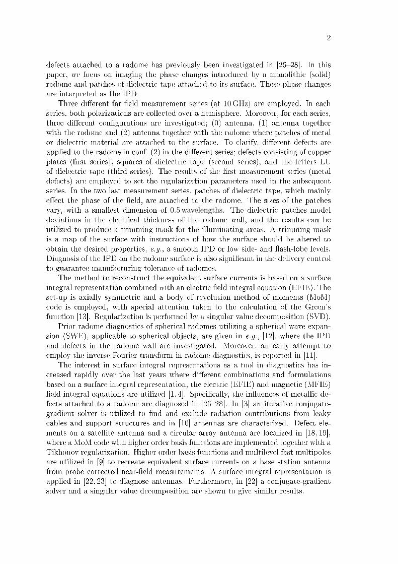
Figure 1: Description and notation of the con�gurations referred to throughout thepaper. The middle �gure shows the unit vectors of the coordinate system in whichthe reconstructed �elds are expressed.
The focus of this paper is radome diagnostics, i.e., to localize patches of dielectrictape attached to its surface from measured far-�eld data. In Section 2.1, the set-up,the compact test range, and the measured far �eld are described. The IPD anddi�erent visualization options � the electric or the magnetic �eld � are discussedin Section 2.2. In Section 3, an outline of the reconstructing algorithm is given.Imaging results are viewed and analyzed in Section 4, whereas conclusions anddiscussions of future possibilities are �nally given in Section 5.
2 Radome diagnostics
A measured far �eld of an antenna and radome con�guration may indicate unwanteddeviations; e.g., increased and changed side lobes, and boresight errors. To �nd theorigin of the errors, diagnostic tools are essential. Here, far-�eld measurements froma compact test range is utilized to localize phase shifts, insertion phase delays (IPD)on the radome surface, caused by the radome and attached patches of dielectrictape.
2.1 Measurement data and set-up
Three di�erent measurement series are conducted at 10 GHz. Each measurementseries consists of three con�gurations; antenna � conf. (0), antenna together withthe radome � conf. (1), and antenna together with the radome where defects areattached to the surface � conf. (2), see Figure 1. Di�erent defects are applied to theradome in conf. (2) in the di�erent series; defects consisting of copper plates (�rstseries), squares of dielectric tape (second series), and the letters LU of dielectrictape (third series). To clarify, conf. (0) and (1) are the same in all three series.
4
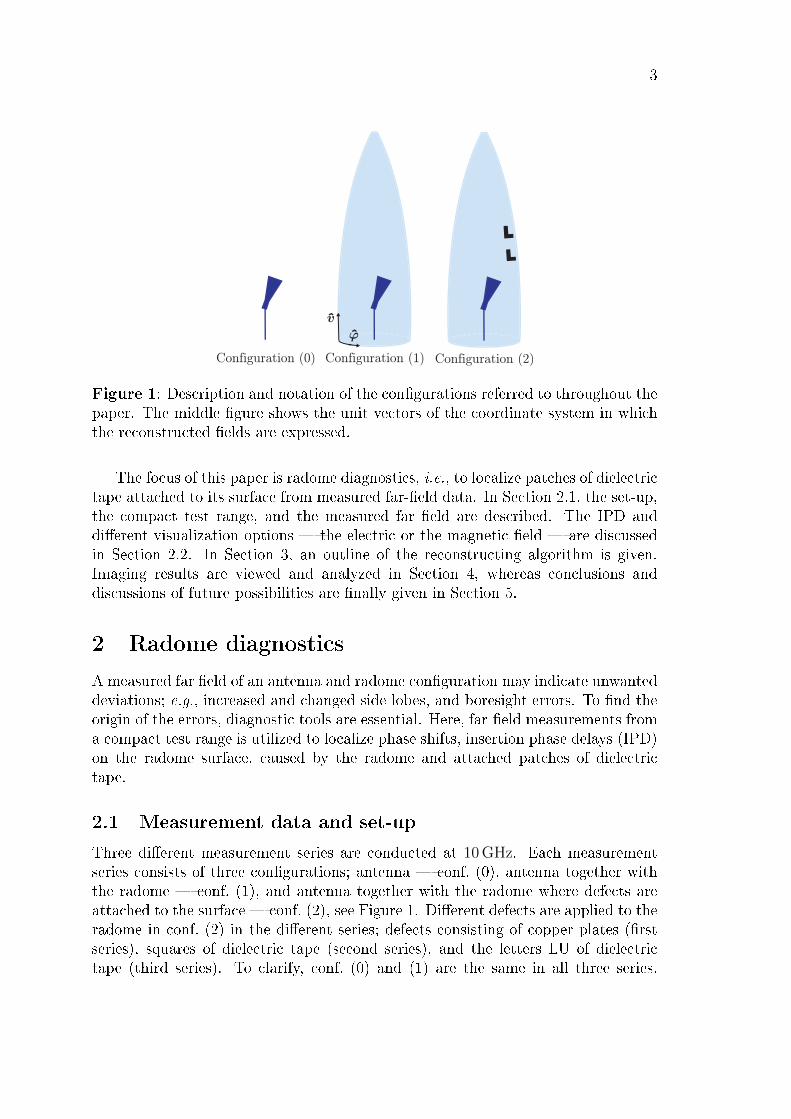
Figure 2: Photo of the measurement set-up in the compact test range.
The reason for doing these all over is that the measurement series were obtainedat di�erent times. In this way, we avoid the in�uence of small deviations in themechanical and electrical set-up together with relative phase and amplitude shiftsbetween the series. The con�guration number is indicated as a superscript on the�elds, whereas the �eld component is showed by a subscript, i.e., H
(0)v = v ·H(0) is
the magnetic component directed along the height of the radome surface when onlythe antenna is present (cf., notation in Figure 1).
The far-�eld measurements were carried out at a compact test range at GKNAerospace Applied Composites, Linköping, Sweden, see Figure 2 [33]. The far �eldis measured on a hemisphere by turning the radome between 0◦ − 90◦ in the polarplane (described by θ) for each azimuthal turn (described by ϕ), where θ and ϕ arestandard spherical coordinates, see Figure 3 for de�nitions and notational system.Measurements in the polar plane are continuously recorded at 1◦/ s, whereas themeasurements along the azimuthal plane are discrete and thereby more time con-suming. The �eld is sampled every second degree in the azimuthal plane and everydegree in the polar plane. A reduction of the sample density by a factor of two inthe polar plane is not noticeable in the imaging results, indicating that the sampledensities are satisfactory [14, 34]. Measuring one con�guration, both polarizations,took approximately nine hours.
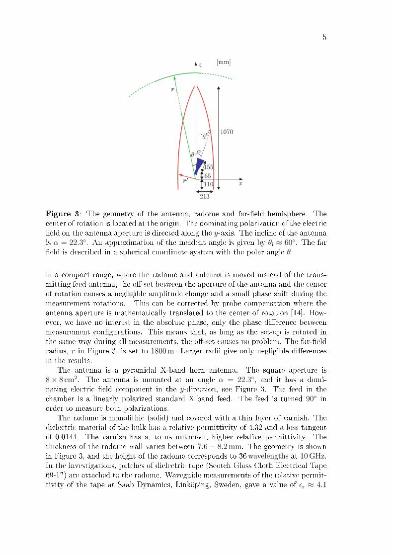
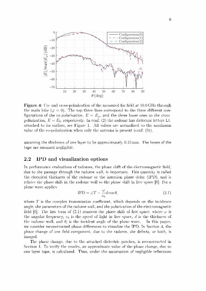
The measured far �eld for both the co- and cross-polarization and the three dif-ferent con�gurations is given in Figure 4, for measurement series number three. The�gure shows a cross section in the polar plane of the �elds through the main lobe,and it is observed that the radome � conf. (1) � changes the far �eld. Attach-ing patches of dielectric tape in the form of the letters LU to the radome surface� conf. (2) � alters the �eld a little more, which is hardly visible in the �gure.Moreover, the origin of the defects can hardly be determined from the far-�eld dataalone. The far �elds of the other two measurement series have similar appearance.
In the far-�eld measurements no probe compensation is necessary [34]. Moreover,
5
[mm]z
x
r
r011065
155
1070
µ
µ
®
i
213
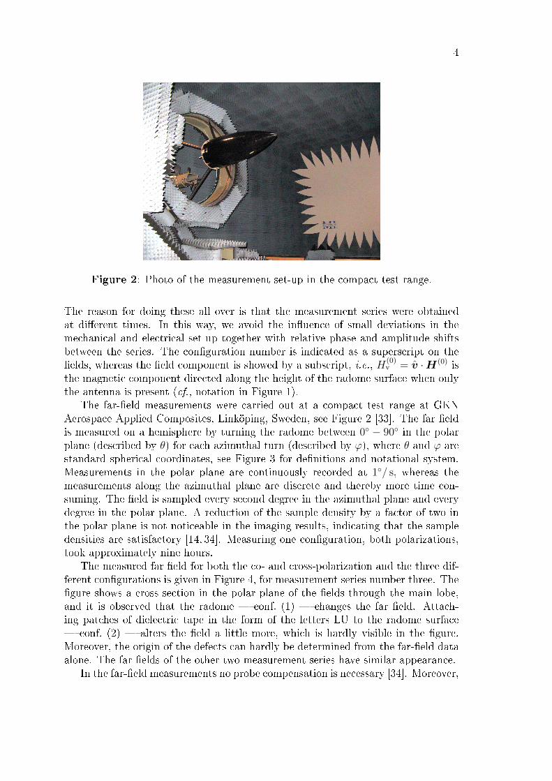
Figure 3: The geometry of the antenna, radome and far-�eld hemisphere. Thecenter of rotation is located at the origin. The dominating polarization of the electric�eld on the antenna aperture is directed along the y-axis. The incline of the antennais α = 22.3◦. An approximation of the incident angle is given by θi ≈ 60◦. The far�eld is described in a spherical coordinate system with the polar angle θ.
in a compact range, where the radome and antenna is moved instead of the trans-mitting feed antenna, the o�-set between the aperture of the antenna and the centerof rotation causes a negligible amplitude change and a small phase shift during themeasurement rotations. This can be corrected by probe compensation where theantenna aperture is mathematically translated to the center of rotation [14]. How-ever, we have no interest in the absolute phase, only the phase di�erence betweenmeasurement con�gurations. This means that, as long as the set-up is rotated inthe same way during all measurements, the o�-set causes no problem. The far-�eldradius, r in Figure 3, is set to 1800 m. Larger radii give only negligible di�erencesin the results.
The antenna is a pyramidal X-band horn antenna. The square aperture is8× 8 cm2. The antenna is mounted at an angle α = 22.3◦, and it has a domi-nating electric �eld component in the y-direction, see Figure 3. The feed in thechamber is a linearly polarized standard X-band feed. The feed is turned 90◦ inorder to measure both polarizations.
The radome is monolithic (solid) and covered with a thin layer of varnish. Thedielectric material of the bulk has a relative permittivity of 4.32 and a loss tangentof 0.0144. The varnish has a, to us unknown, higher relative permittivity. Thethickness of the radome wall varies between 7.6 − 8.2 mm. The geometry is shownin Figure 3, and the height of the radome corresponds to 36wavelengths at 10 GHz.In the investigations, patches of dielectric tape (Scotch Glass Cloth Electrical Tape69-1") are attached to the radome. Waveguide measurements of the relative permit-tivity of the tape at Saab Dynamics, Linköping, Sweden, gave a value of εr ≈ 4.1
6
10 20 30 40 50 60 70 80 90
−70
−60
−50
−40
−30
−20
−10
0
Configuration(0)Configuration(1)Configuration(2)
θ (deg)
|E|/max|E
ϕ|(
dB
)
Figure 4: Co- and cross-polarization of the measured far �eld at 10.0 GHz throughthe main lobe (ϕ = 0). The top three lines correspond to the three di�erent con-�gurations of the co-polarization, E = Eϕ, and the three lower ones to the cross-polarization, E = Eθ, respectively. In conf. (2) the radome has dielectric letters LUattached to its surface, see Figure 1. All values are normalized to the maximumvalue of the co-polarization when only the antenna is present (conf. (0)).
assuming the thickness of one layer to be approximately 0.15 mm. The losses of thetape are assumed negligible.
2.2 IPD and visualization options
In performance evaluations of radomes, the phase shift of the electromagnetic �eld,due to the passage through the radome wall, is important. This quantity is calledthe electrical thickness of the radome or the insertion phase delay (IPD), and itrelates the phase shift in the radome wall to the phase shift in free space [6]. For aplane wave applies
IPD = ∠T − ω
c0d cos θi (2.1)
where T is the complex transmission coe�cient, which depends on the incidenceangle, the parameters of the radome wall, and the polarization of the electromagnetic�eld [6]. The last term of (2.1) removes the phase shift of free space, where ω isthe angular frequency, c0 is the speed of light in free space, d is the thickness ofthe radome wall, and θi is the incident angle of the plane wave. In this paper,we consider reconstructed phase di�erences to visualize the IPD. In Section 4, thephase change of one �eld component, due to the radome, the defects, or both, isimaged.
The phase change, due to the attached dielectric patches, is reconstructed inSection 4. To verify the results, an approximate value of the phase change, due toone layer tape, is calculated. Thus, under the assumption of negligible re�ections
7
0.20 0.25 0.30 0.35
0.45
0.50
0.55
0.60
0
5
10
15
(a)
horizontal arc length (m)
vertical
arclength(m
)∠H(1)
v − ∠H(2)v (deg)
0.20 0.25 0.30 0.35
0.45
0.50
0.55
0.60
0
5
10
15
(b)
horizontal arc length (m)
vertical
arclength(m
)
∠E(1)ϕ − ∠E(2)
ϕ (deg)
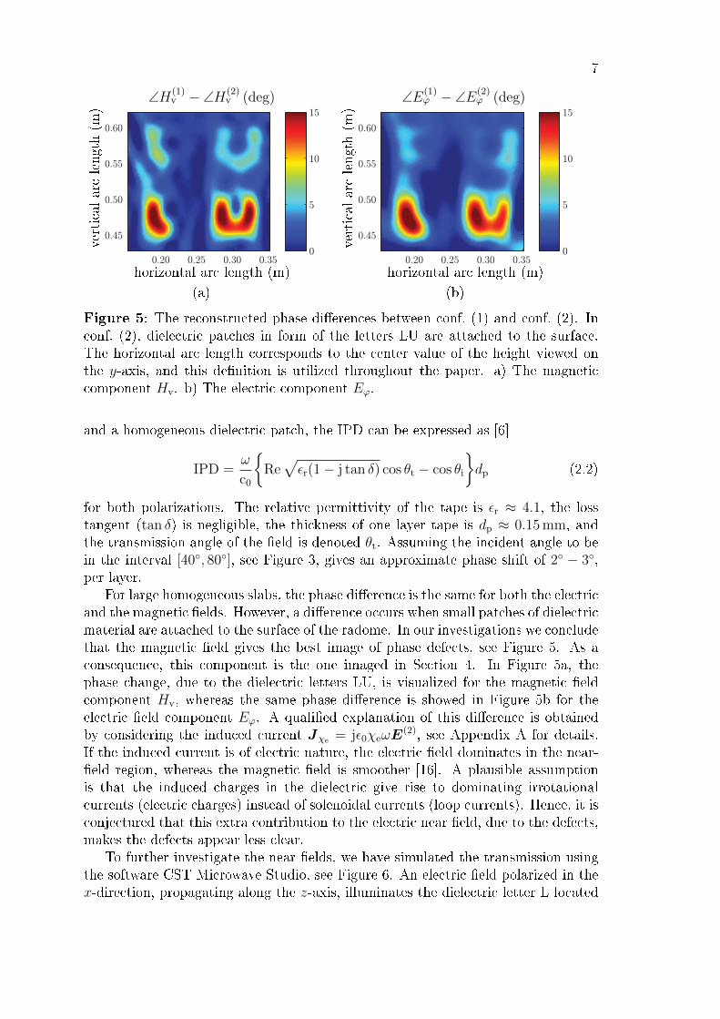
Figure 5: The reconstructed phase di�erences between conf. (1) and conf. (2). Inconf. (2), dielectric patches in form of the letters LU are attached to the surface.The horizontal arc length corresponds to the center value of the height viewed onthe y-axis, and this de�nition is utilized throughout the paper. a) The magneticcomponent Hv. b) The electric component Eϕ.
and a homogeneous dielectric patch, the IPD can be expressed as [6]
IPD =ω
c0
{Re√εr(1− j tan δ) cos θt − cos θi
}dp (2.2)
for both polarizations. The relative permittivity of the tape is εr ≈ 4.1, the losstangent (tan δ) is negligible, the thickness of one layer tape is dp ≈ 0.15 mm, andthe transmission angle of the �eld is denoted θt. Assuming the incident angle to bein the interval [40◦, 80◦], see Figure 3, gives an approximate phase shift of 2◦ − 3◦,per layer.
For large homogeneous slabs, the phase di�erence is the same for both the electricand the magnetic �elds. However, a di�erence occurs when small patches of dielectricmaterial are attached to the surface of the radome. In our investigations we concludethat the magnetic �eld gives the best image of phase defects, see Figure 5. As aconsequence, this component is the one imaged in Section 4. In Figure 5a, thephase change, due to the dielectric letters LU, is visualized for the magnetic �eldcomponent Hv, whereas the same phase di�erence is showed in Figure 5b for theelectric �eld component Eϕ. A quali�ed explanation of this di�erence is obtainedby considering the induced current Jχe = jε0χeωE
(2), see Appendix A for details.If the induced current is of electric nature, the electric �eld dominates in the near-�eld region, whereas the magnetic �eld is smoother [16]. A plausible assumptionis that the induced charges in the dielectric give rise to dominating irrotationalcurrents (electric charges) instead of solenoidal currents (loop currents). Hence, it isconjectured that this extra contribution to the electric near �eld, due to the defects,makes the defects appear less clear.
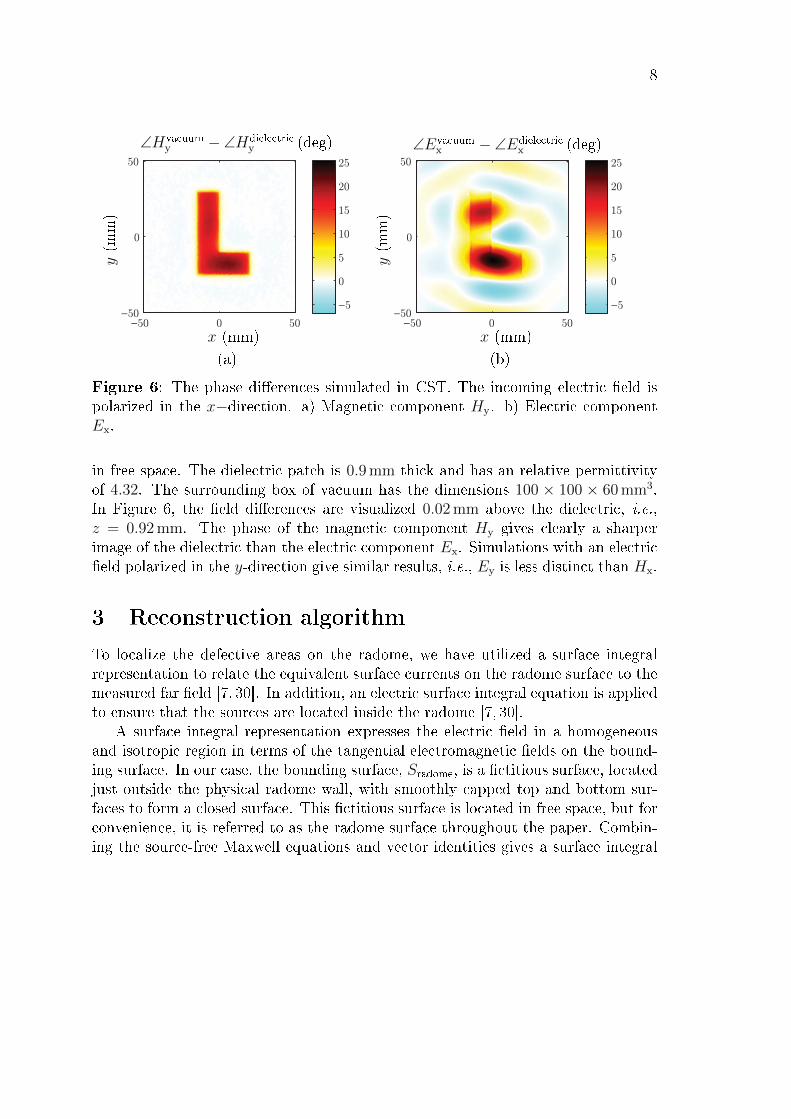
To further investigate the near �elds, we have simulated the transmission usingthe software CST Microwave Studio, see Figure 6. An electric �eld polarized in thex-direction, propagating along the z-axis, illuminates the dielectric letter L located
8
−50 0 50−50
0
50
−5
0
5
10
15
20
25
(a)
x (mm)
y(m
m)
∠Hvacuum
y − ∠Hdielectric
y (deg)
−50 0 50−50
0
50
−5
0
5
10
15
20
25
(b)
x (mm)
y(m
m)
∠Evacuum
x − ∠Edielectric
x (deg)
Figure 6: The phase di�erences simulated in CST. The incoming electric �eld ispolarized in the x−direction. a) Magnetic component Hy. b) Electric componentEx.
in free space. The dielectric patch is 0.9 mm thick and has an relative permittivityof 4.32. The surrounding box of vacuum has the dimensions 100 × 100 × 60 mm3.In Figure 6, the �eld di�erences are visualized 0.02 mm above the dielectric, i.e.,z = 0.92 mm. The phase of the magnetic component Hy gives clearly a sharperimage of the dielectric than the electric component Ex. Simulations with an electric�eld polarized in the y-direction give similar results, i.e., Ey is less distinct than Hx.
3 Reconstruction algorithm
To localize the defective areas on the radome, we have utilized a surface integralrepresentation to relate the equivalent surface currents on the radome surface to themeasured far �eld [7, 30]. In addition, an electric surface integral equation is appliedto ensure that the sources are located inside the radome [7, 30].
A surface integral representation expresses the electric �eld in a homogeneousand isotropic region in terms of the tangential electromagnetic �elds on the bound-ing surface. In our case, the bounding surface, Sradome, is a �ctitious surface, locatedjust outside the physical radome wall, with smoothly capped top and bottom sur-faces to form a closed surface. This �ctitious surface is located in free space, but forconvenience, it is referred to as the radome surface throughout the paper. Combin-ing the source-free Maxwell equations and vector identities gives a surface integral
9
representation of the electric �eld [25, 30]∫∫Sradome
(−jkη0 g(r′, r)
[n(r′)×H(r′)
]− η0
jk∇′g(r′, r)
{∇′S ·
[n(r′)×H(r′)
]}
−∇′g(r′, r)×[n(r′)×E(r′)
])dS ′ =
{E(r) r outside Sradome
0 r inside Sradome
(3.1)for the exterior problem where all the sources are located inside Sradome. The usedtime convention is ejωt, ω is the angular frequency, and η0 is the intrinsic waveimpedance of free space. The surface divergence is denoted ∇S· [8], the unit normal
n points outward, and the scalar free-space Green's function is g(r′, r) = e−jk|r−r′|
4π|r−r′| ,
where the wave number is k = ω/c0 and c0 is the speed of light in free space. Therepresentation (3.1) states that if the electromagnetic �eld on a bounding surfaceis known, the electromagnetic �eld in the volume, outside of Sradome, can be deter-mined [30]. If these integrals are evaluated at a point r lying in the volume enclosedby Sradome, these integrals cancel each other (extinction).
The representation (3.1) consists of three components, two tangential �elds andone normal component of the �eld. Since the normal component can be determinedby the knowledge of the tangential parts, this representation contains redundancies.As a consequence, specifying only the tangential components su�ce [25]. The mea-sured far �eld consists of two orthogonal components, ϕ (azimuth) and θ (polar).The tangential �elds on the radome surface are decomposed into two tangentialcomponents along the horizontal, ϕ, and vertical, v, arc lengths coordinates, seeFigure 1. The lower representation in (3.1) is transformed into a surface integralequation letting r approach Sradome from the inside [8, 30]. To simplify, the operatorsL and K are introduced as [17]
L(X)(r) = jk
∫∫Sradome
{g(r′, r)X(r′)− 1
k2∇′g(r′, r)
[∇′S ·X(r′)
]}dS ′
K(X)(r) =
∫∫Sradome
∇′g(r′, r)×X(r′) dS ′(3.2)
In this notation the surface integral representation and the surface integral equa-tion for the electric �eld (EFIE) yield[
θ(r)ϕ(r)
]·{−L (η0J) (r) +K (M ) (r)
}=
[θ(r) ·E(r)ϕ(r) ·E(r)
]r ∈ Smeas (3.3)
n(r)×{L (η0J) (r)−K (M ) (r)
}=
1
2M(r) r ∈ Sradome (3.4)
where Smeas is the set of discrete sample points (cf., Figure 3), and Sradome is the�ctitious surface located precisely outside the physical radome wall with a smoothly

10
capped top and bottom. In a similar manner, a surface integral equation of themagnetic �eld (MFIE) can be derived,
n(r)×{L (M ) (r) +K (η0J) (r)
}= −η0
2J(r) r ∈ Sradome (3.5)
In (3.3)�(3.5) we have introduced the equivalent surface currents on the radomesurface, J = n×H andM = −n×E [17]. As mentioned above, the tangential �eldson the radome surface are decomposed into two components along the horizontal andvertical arc lengths coordinates of the surface, that is [ϕ, v, n] forms a right-handedcoordinate system. Throughout the paper we use the notations, Hv = H · v = −Jϕ,Hϕ = H · ϕ = Jv, Ev = E · v = Mϕ, and Eϕ = E · ϕ = −Mv for the reconstructedtangential electromagnetic �elds.
The representation (3.3) can be used together with EFIE (3.4), MFIE (3.5), or acombination of both (CFIE), to avoid internal resonances [5, 7]. We have solved theproblem by using both EFIE and MFIE separately together with the representation.The results do not di�er signi�cantly from each other. As a consequence, there are noproblems with internal resonances for the employed set-up and choice of operators,since the internal resonance frequencies of EFIE and MFIE di�er [5]. In Section 4,the results using (3.3) together with (3.4) are visualized.
The surface integral equations are written in their weak forms, i.e., they aremultiplied with a test function and integrated over their domain [5, 21]. The set-up, see Figure 3, is axially symmetric. Consequently, a Fourier expansion reducesthe problem by one dimension [24]. Only the Fourier components of the �elds withFourier index m = [−40, 40] are relevant, since the amplitudes of the �eld di�erencesof higher modes are below −60 dB, for all measurement series and con�gurations.Convergence studies show that this choice is su�cient.
The system of equations in (3.3)�(3.5) is solved by a body of revolution methodof moments (MoM) code [2, 24]. The evaluation of the Green's functions is basedon [13]. The basis function in the ϕ-direction consists of a piecewise constant func-tion, and a global function, a Fourier basis, of coordinate ϕ. Moreover, the ba-sis function in the v-direction consists of a piecewise linear function, 1D rooftop,of the coordinate v, and the same global function as the basis function in the ϕ-direction, see Figure 1 for notation. Test functions are chosen according to Galerkin'smethod [5], and the height (arc length) is uniformly discredited in steps of λ/12.The surface is described by a second order approximation.The in-house MoM code isveri�ed by scattering of perfect electric conductors (PEC) and dielectric spheres [32].
The problem is regularized by a singular value decomposition (SVD), where thein�uence of small singular values is reduced [15]. A reference measurement seriesis performed to set the regularizing parameter used in the subsequent series, seeSection 4.1. The inversion of the matrix system is veri�ed using synthetic data.Moreover, the results, which localize the given defects, serve as good veri�cations.
The described method are applied in [26�28], to reconstruct equivalent surfacecurrents from a measured near �eld. A slightly di�erent approach is found in [18, 19].Speci�cally, the surface integral representation, the EFIE, and the MFIE are solvedutilizing higher order bases functions in a MoM solver with a Tikhonov regulariza-tion. In [3, 4, 10], the EFIE and MFIE are evaluated on a surface located inside the
11
surface of reconstruction, and the matrix system is solved by an iterative conjugate-gradient solver. Yet another approach is given in [1, 22, 23], where a surface integralrepresentation is employed together with a conjugate-gradient solver as well as asingular value decomposition. In [9] the authors make use of dyadic Green's func-tions.
4 Reconstruction results
Three di�erent con�gurations are investigated at 10 GHz; (0) antenna, (1) antennatogether with the radome, and (2) antenna together with the radome where patchesof metal or dielectric material are attached to the surface, see Figure 1. The �eld ismeasured in the far-�eld region, as described in Section 2.1. The equivalent surfacecurrents, both amplitude and phase, are reconstructed on a �ctitious surface shapedas the radome. Observe, even in the case when only the antenna is present �conf. (0) � the �eld is reconstructed on a radome shaped surface.
The magnetic component, Hv, is analyzed in this section, since it gives thesharpest image of the phase shifts (cf., the discussion in Section 2.2). Moreover, thecomponents Hϕ and Ev are small cross-polarization terms, and a pronounced in�u-ence of the phase shift due to a thin dielectric patch of tape are not visible in thesecomponents. For this reason, these components are not investigated. The notationused in visualizing the phase di�erence between the �elds from e.g., conf. (1) and
(2), is ∠H(1)v −∠H(2)
v = 180π∠{H
(1)v [H
(2)v ]∗
}, where the star denotes the complex con-
jugate. The employed time convention, ejωt, gives a negative phase shift, indicatingthat ∠H(1)
v − ∠H(2)v > 0◦.
4.1 Reference measurement
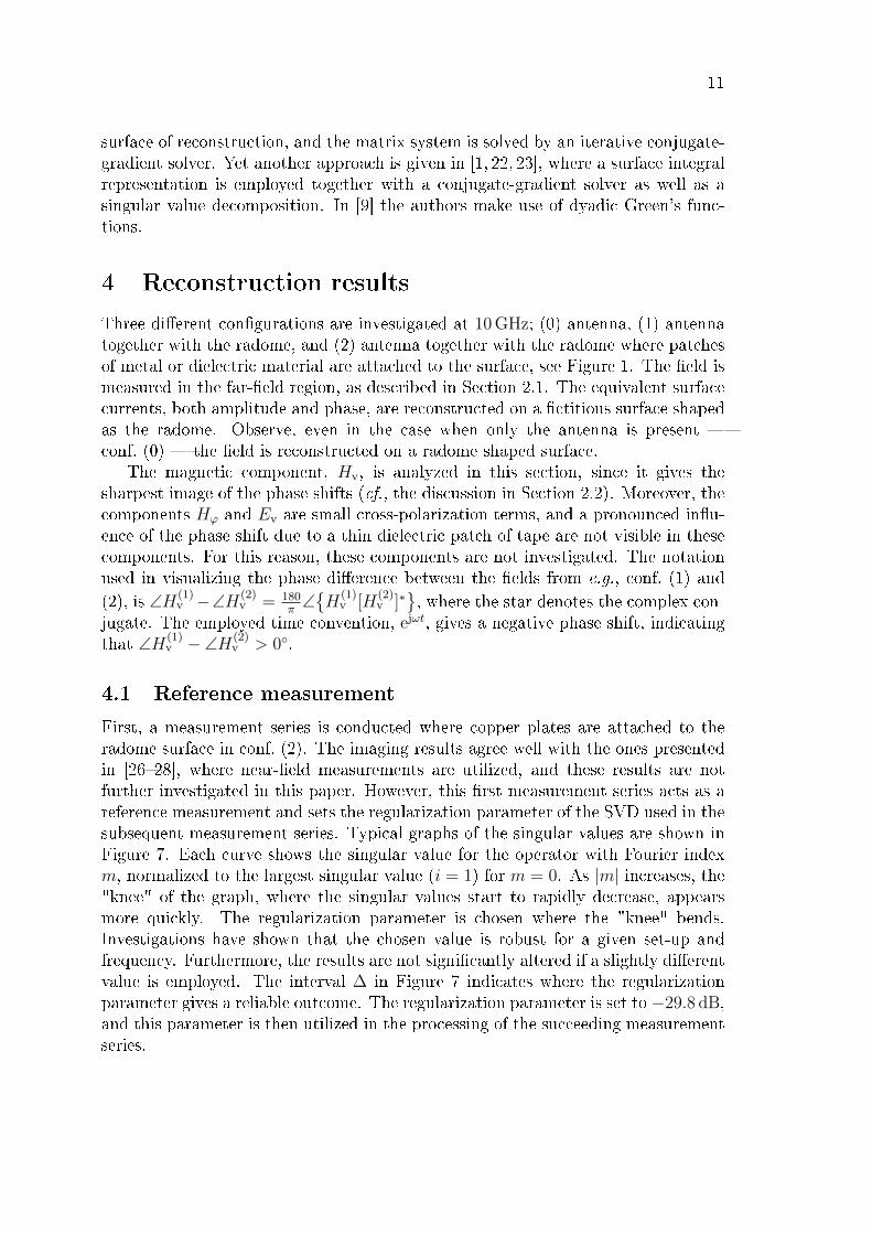
First, a measurement series is conducted where copper plates are attached to theradome surface in conf. (2). The imaging results agree well with the ones presentedin [26�28], where near-�eld measurements are utilized, and these results are notfurther investigated in this paper. However, this �rst measurement series acts as areference measurement and sets the regularization parameter of the SVD used in thesubsequent measurement series. Typical graphs of the singular values are shown inFigure 7. Each curve shows the singular value for the operator with Fourier indexm, normalized to the largest singular value (i = 1) for m = 0. As |m| increases, the"knee" of the graph, where the singular values start to rapidly decrease, appearsmore quickly. The regularization parameter is chosen where the "knee" bends.Investigations have shown that the chosen value is robust for a given set-up andfrequency. Furthermore, the results are not signi�cantly altered if a slightly di�erentvalue is employed. The interval ∆ in Figure 7 indicates where the regularizationparameter gives a reliable outcome. The regularization parameter is set to −29.8 dB,and this parameter is then utilized in the processing of the succeeding measurementseries.
12
20 40 60 80 100 120−100
−80
−60
−40
−20
0
¢
i
σm i/σ
0 1(d
B)
Figure 7: Singular values σmi . Each curve depicts di�erent Fourier index m, andthe curves are normalized to the largest singular value for m = 0. The interval, ∆,where the regularization parameter gives a reliable outcome, is drawn.
4.2 Imaging of dielectric material
Obtaining a constant phase shift over the illuminated area is often important totrim radomes. The trimming is achieved by adding or removing dielectric materialto the radome surface. To investigate if the proposed method can be utilized tomap areas of the radome surface with a deviating electrical thickness, patches ofdielectric material (defects), are attached to the radome surface in conf. (2). Defectsof dielectric material mainly a�ect the phase of the �eld, and the phase di�erencesof the �elds for the di�erent con�gurations give us an understanding of how thedefects delay the �elds.
Measurement series number two and three are employed. In each series the �eldfrom the antenna (conf. (0)), the antenna together with the radome (conf. (1)),and the antenna together with the radome where dielectric patches are attached tothe surface (conf. (2)), were measured, cf., Figure 1. In the second measurementseries, squares are added to the area where the main lobe illuminates the radome,see Figure 8a, where the size and the thickness of the patches are shown. In thethird measurement series, the letters LU are attached to the radome, see Figure 8b.
4.2.1 Dielectric squares
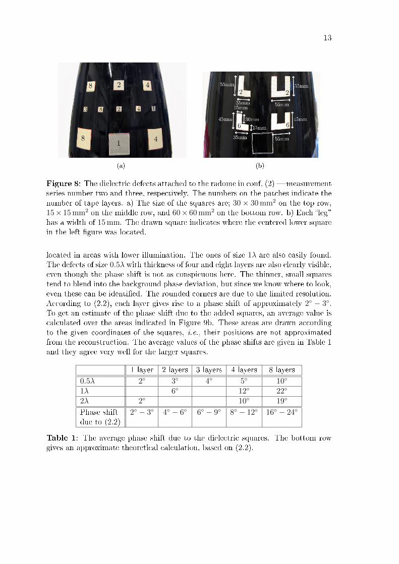
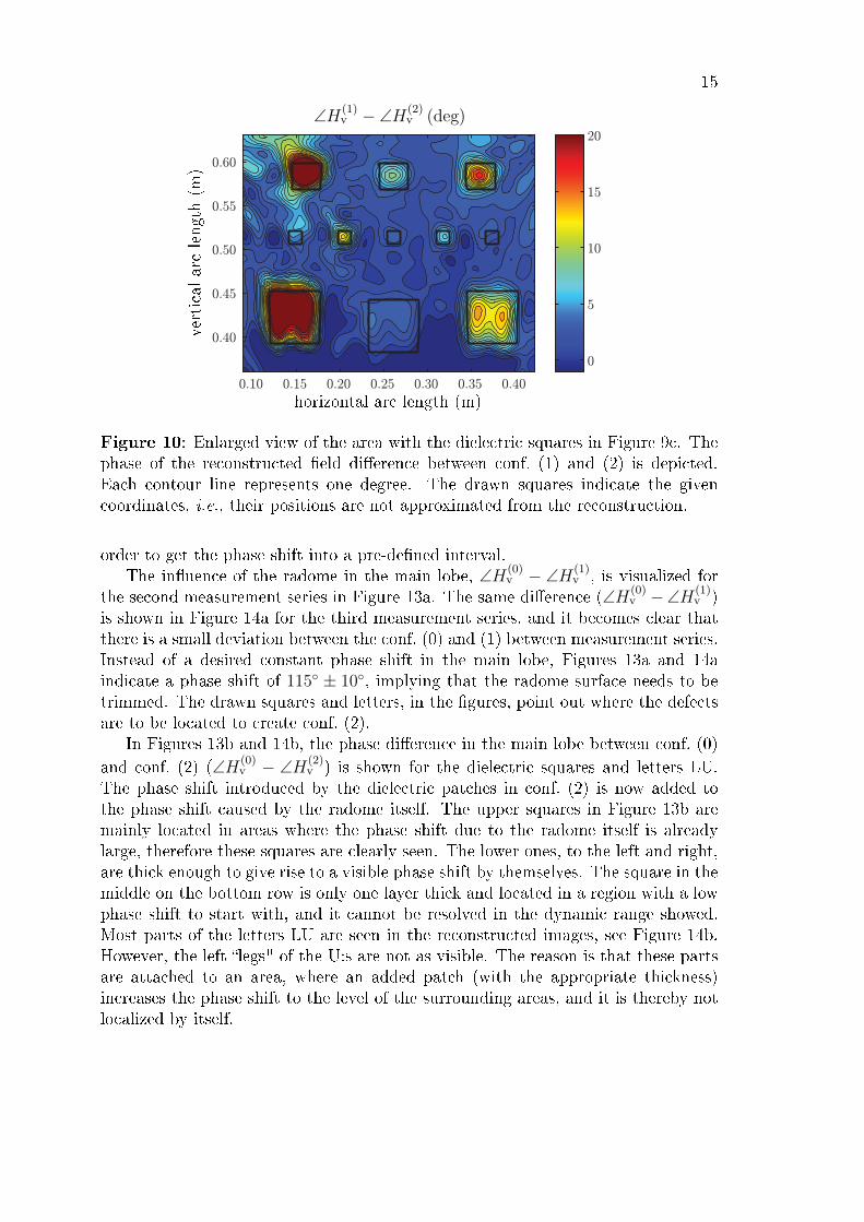
Eleven dielectric squares of the sizes 0.5λ, 1λ, and 2λ are added to the radomesurface, see Figures 8a and 9. In Figure 9b, the illumination of the area of conf. (1),to which the dielectric squares will be applied to create one case of conf. (2), isshown. The largest squares are located in a �eld region of [−23,−6] dB, the middlesized in the region [−12, 0.3] dB and the smallest ones in [−9, 0.3] dB, respectively. In
Figures 9c and 10, the reconstructed phase shifts due to the defects, ∠H(1)v −∠H(2)
v ,are visualized. The squares of size 2λ are clearly visible even though they are partly
13
(a) (b)
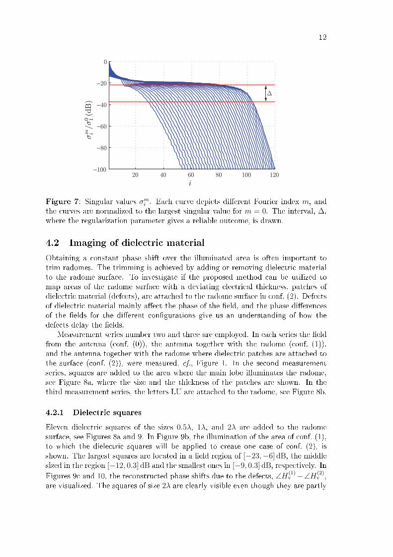
Figure 8: The dielectric defects attached to the radome in conf. (2) � measurementseries number two and three, respectively. The numbers on the patches indicate thenumber of tape layers. a) The size of the squares are; 30× 30 mm2 on the top row,15× 15 mm2 on the middle row, and 60× 60 mm2 on the bottom row. b) Each �leg"has a width of 15 mm. The drawn square indicates where the centered lower squarein the left �gure was located.
located in areas with lower illumination. The ones of size 1λ are also easily found.The defects of size 0.5λ with thickness of four and eight layers are also clearly visible,even though the phase shift is not as conspicuous here. The thinner, small squarestend to blend into the background phase deviation, but since we know where to look,even these can be identi�ed. The rounded corners are due to the limited resolution.According to (2.2), each layer gives rise to a phase shift of approximately 2◦ − 3◦.To get an estimate of the phase shift due to the added squares, an average value iscalculated over the areas indicated in Figure 9b. These areas are drawn accordingto the given coordinates of the squares, i.e., their positions are not approximatedfrom the reconstruction. The average values of the phase shifts are given in Table 1and they agree very well for the larger squares.
1 layer 2 layers 3 layers 4 layers 8 layers
0.5λ 2◦ 3◦ 4◦ 5◦ 10◦
1λ 6◦ 12◦ 22◦
2λ 2◦ 10◦ 19◦
Phase shift 2◦ − 3◦ 4◦ − 6◦ 6◦ − 9◦ 8◦ − 12◦ 16◦ − 24◦
due to (2.2)
Table 1: The average phase shift due to the dielectric squares. The bottom rowgives an approximate theoretical calculation, based on (2.2).
14
(a)
−40
−35
−30
−25
−20
−15
−10
−5
0
(b)
|H(1)v |/max|H(1)
v | (dB)
0
4
8
12
16
20
(c)
∠H(1)v − ∠H(2)
v (deg)
Figure 9: a) A photo of the radome with the dielectric squares (defects). b) The re-constructed �eld, Hv, on the radome � conf. (1). The drawn squares indicate wherethe defects will be located to create conf. (2). c) The phase of the reconstructed�eld di�erence between conf. (1) and (2).
4.2.2 Dielectric letters LU
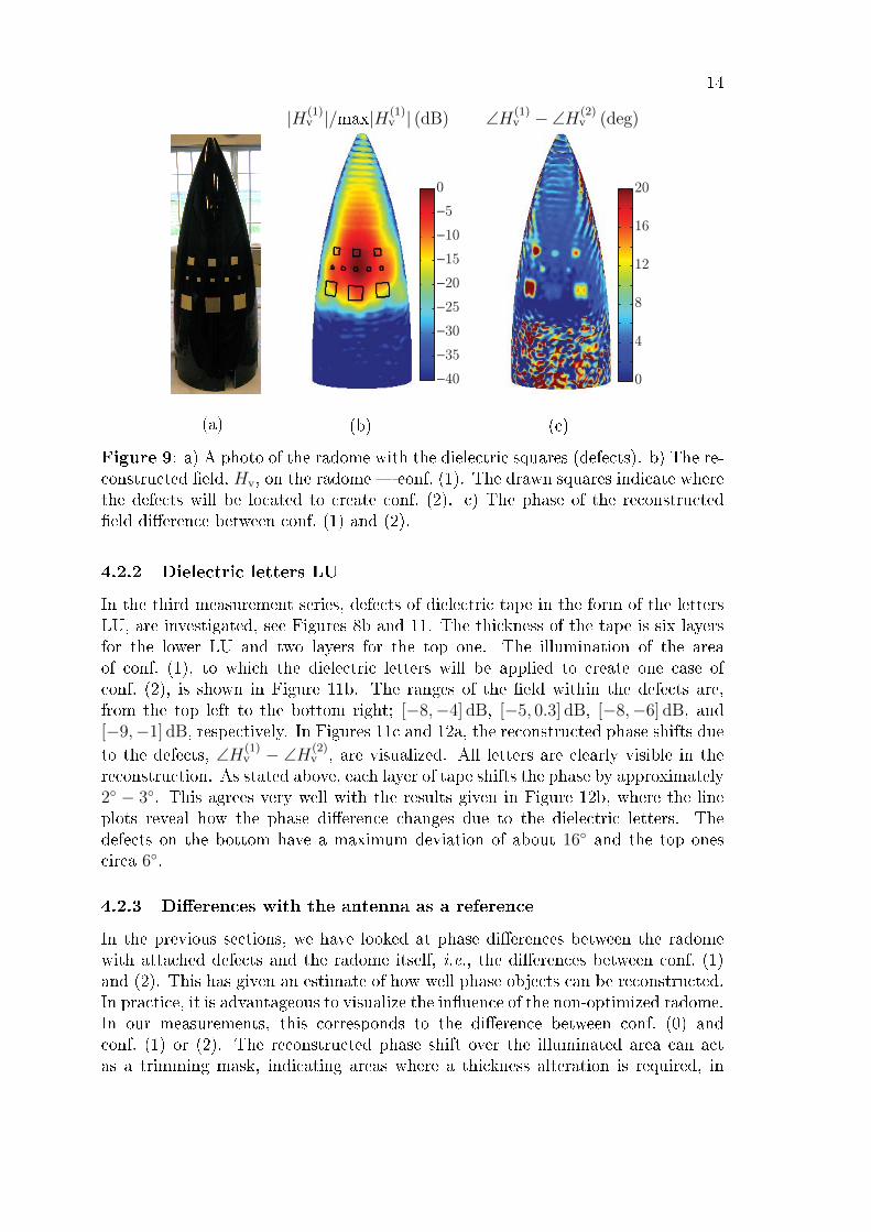
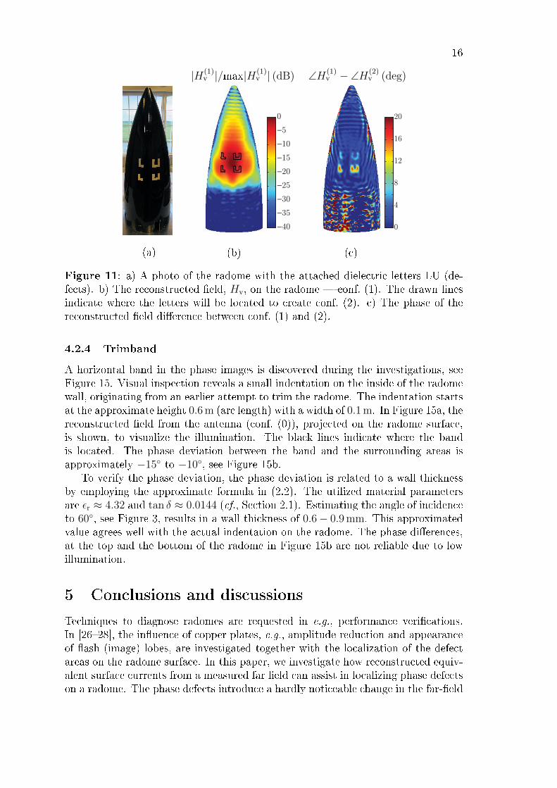
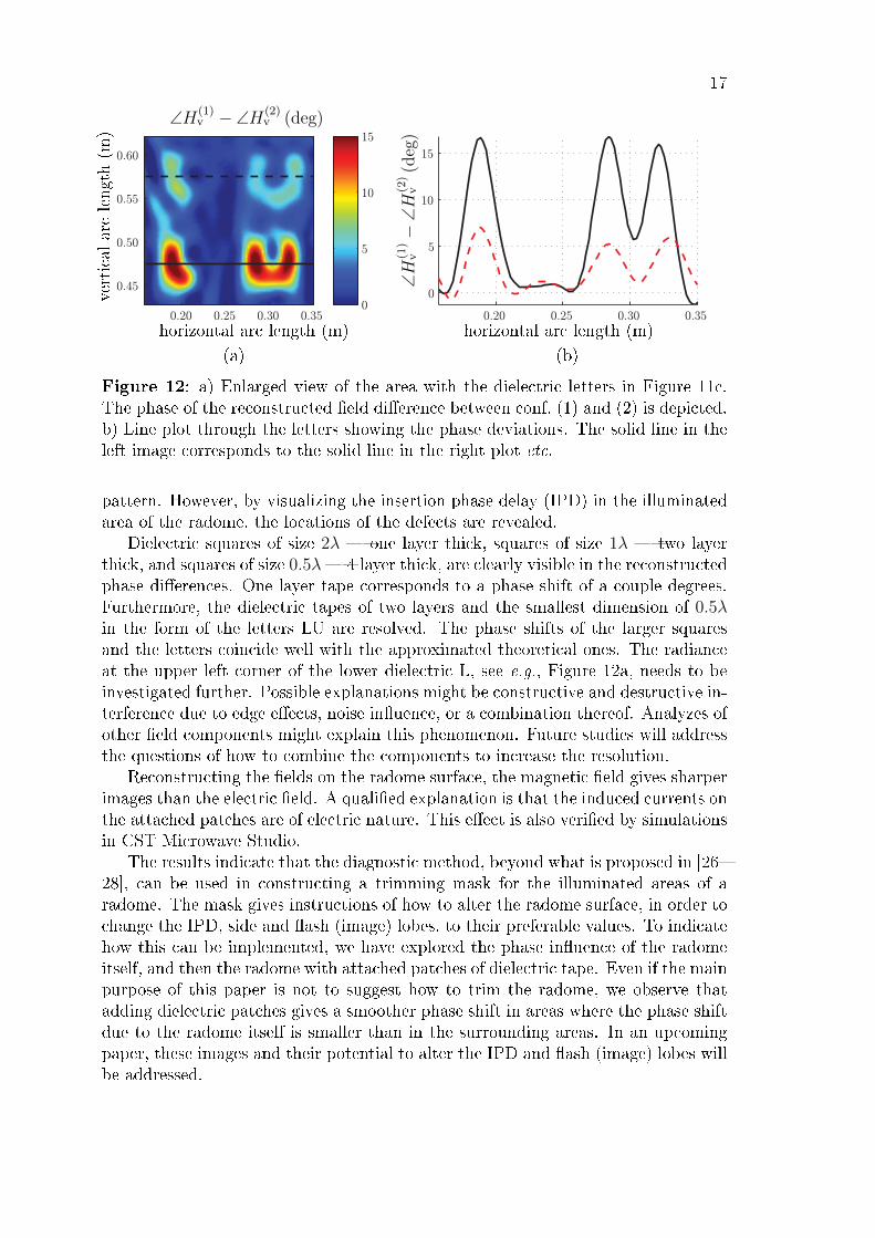
In the third measurement series, defects of dielectric tape in the form of the lettersLU, are investigated, see Figures 8b and 11. The thickness of the tape is six layersfor the lower LU and two layers for the top one. The illumination of the areaof conf. (1), to which the dielectric letters will be applied to create one case ofconf. (2), is shown in Figure 11b. The ranges of the �eld within the defects are,from the top left to the bottom right; [−8,−4] dB, [−5, 0.3] dB, [−8,−6] dB, and[−9,−1] dB, respectively. In Figures 11c and 12a, the reconstructed phase shifts due
to the defects, ∠H(1)v − ∠H(2)
v , are visualized. All letters are clearly visible in thereconstruction. As stated above, each layer of tape shifts the phase by approximately2◦ − 3◦. This agrees very well with the results given in Figure 12b, where the lineplots reveal how the phase di�erence changes due to the dielectric letters. Thedefects on the bottom have a maximum deviation of about 16◦ and the top onescirca 6◦.
4.2.3 Di�erences with the antenna as a reference
In the previous sections, we have looked at phase di�erences between the radomewith attached defects and the radome itself, i.e., the di�erences between conf. (1)and (2). This has given an estimate of how well phase objects can be reconstructed.In practice, it is advantageous to visualize the in�uence of the non-optimized radome.In our measurements, this corresponds to the di�erence between conf. (0) andconf. (1) or (2). The reconstructed phase shift over the illuminated area can actas a trimming mask, indicating areas where a thickness alteration is required, in
15
0.10 0.15 0.20 0.25 0.30 0.35 0.40
0.40
0.45
0.50
0.55
0.60
0
5
10
15
20
horizontal arc length (m)
vertical
arclength(m
)
∠H(1)v − ∠H(2)
v (deg)
Figure 10: Enlarged view of the area with the dielectric squares in Figure 9c. Thephase of the reconstructed �eld di�erence between conf. (1) and (2) is depicted.Each contour line represents one degree. The drawn squares indicate the givencoordinates, i.e., their positions are not approximated from the reconstruction.
order to get the phase shift into a pre-de�ned interval.The in�uence of the radome in the main lobe, ∠H(0)
v − ∠H(1)v , is visualized for
the second measurement series in Figure 13a. The same di�erence (∠H(0)v −∠H(1)
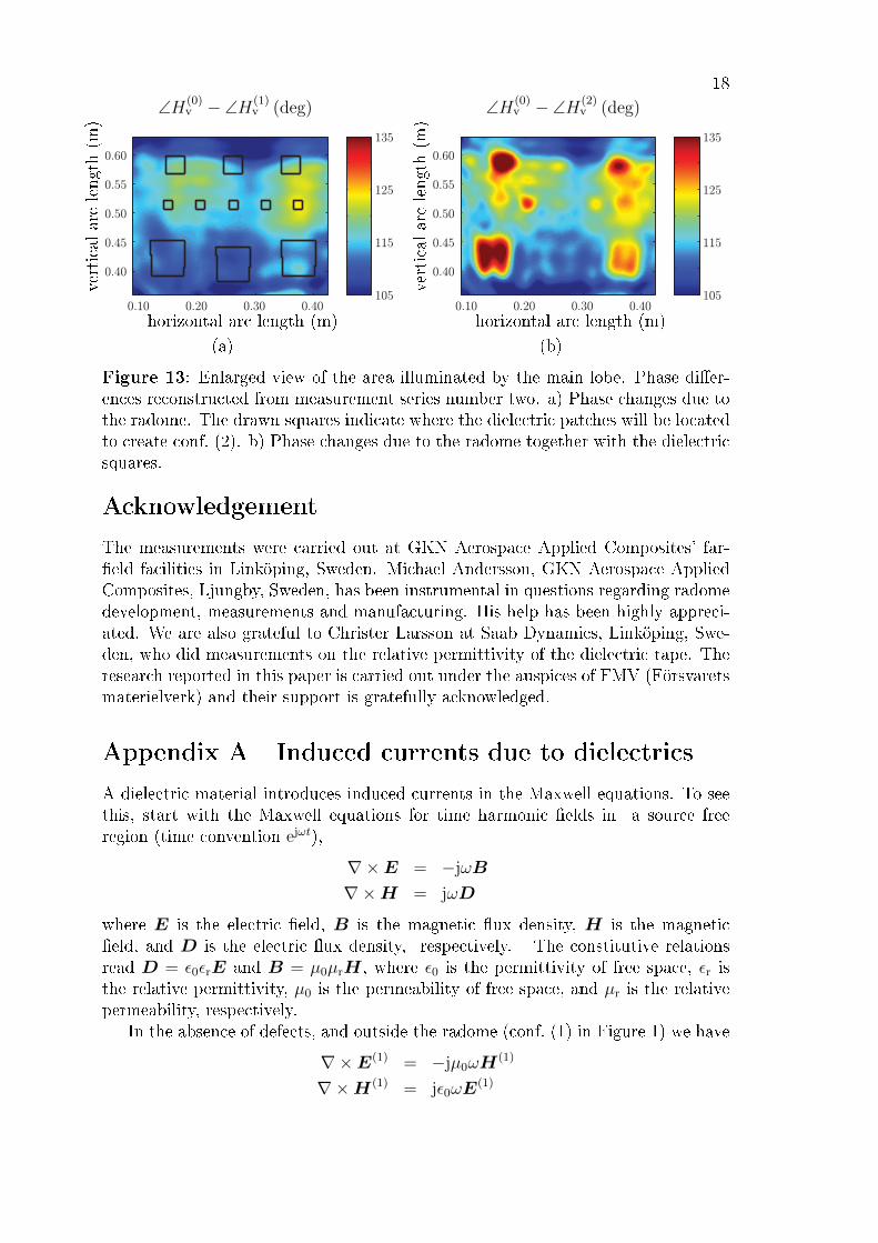
v )is shown in Figure 14a for the third measurement series, and it becomes clear thatthere is a small deviation between the conf. (0) and (1) between measurement series.Instead of a desired constant phase shift in the main lobe, Figures 13a and 14aindicate a phase shift of 115◦ ± 10◦, implying that the radome surface needs to betrimmed. The drawn squares and letters, in the �gures, point out where the defectsare to be located to create conf. (2).
In Figures 13b and 14b, the phase di�erence in the main lobe between conf. (0)
and conf. (2) (∠H(0)v − ∠H(2)
v ) is shown for the dielectric squares and letters LU.The phase shift introduced by the dielectric patches in conf. (2) is now added tothe phase shift caused by the radome itself. The upper squares in Figure 13b aremainly located in areas where the phase shift due to the radome itself is alreadylarge, therefore these squares are clearly seen. The lower ones, to the left and right,are thick enough to give rise to a visible phase shift by themselves. The square in themiddle on the bottom row is only one layer thick and located in a region with a lowphase shift to start with, and it cannot be resolved in the dynamic range showed.Most parts of the letters LU are seen in the reconstructed images, see Figure 14b.However, the left �legs" of the U:s are not as visible. The reason is that these partsare attached to an area, where an added patch (with the appropriate thickness)increases the phase shift to the level of the surrounding areas, and it is thereby notlocalized by itself.
16
(a)
−40
−35
−30
−25
−20
−15
−10
−5
0
(b)
|H(1)v |/max|H(1)
v | (dB)
0
4
8
12
16
20
(c)
∠H(1)v − ∠H(2)
v (deg)
Figure 11: a) A photo of the radome with the attached dielectric letters LU (de-fects). b) The reconstructed �eld, Hv, on the radome � conf. (1). The drawn linesindicate where the letters will be located to create conf. (2). c) The phase of thereconstructed �eld di�erence between conf. (1) and (2).
4.2.4 Trimband
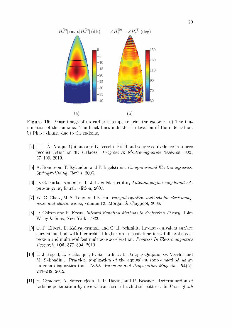
A horizontal band in the phase images is discovered during the investigations, seeFigure 15. Visual inspection reveals a small indentation on the inside of the radomewall, originating from an earlier attempt to trim the radome. The indentation startsat the approximate height 0.6 m (arc length) with a width of 0.1 m. In Figure 15a, thereconstructed �eld from the antenna (conf. (0)), projected on the radome surface,is shown, to visualize the illumination. The black lines indicate where the bandis located. The phase deviation between the band and the surrounding areas isapproximately −15◦ to −10◦, see Figure 15b.
To verify the phase deviation, the phase deviation is related to a wall thicknessby employing the approximate formula in (2.2). The utilized material parametersare εr ≈ 4.32 and tan δ ≈ 0.0144 (cf., Section 2.1). Estimating the angle of incidenceto 60◦, see Figure 3, results in a wall thickness of 0.6− 0.9 mm. This approximatedvalue agrees well with the actual indentation on the radome. The phase di�erences,at the top and the bottom of the radome in Figure 15b are not reliable due to lowillumination.
5 Conclusions and discussions
Techniques to diagnose radomes are requested in e.g., performance veri�cations.In [26�28], the in�uence of copper plates, e.g., amplitude reduction and appearanceof �ash (image) lobes, are investigated together with the localization of the defectareas on the radome surface. In this paper, we investigate how reconstructed equiv-alent surface currents from a measured far �eld can assist in localizing phase defectson a radome. The phase defects introduce a hardly noticeable change in the far-�eld
17
0.20 0.25 0.30 0.35
0.45
0.50
0.55
0.60
0
5
10
15
(a)
horizontal arc length (m)
vertical
arclength(m
)∠H(1)
v − ∠H(2)v (deg)
0.20 0.25 0.30 0.35
0
5
10
15
(b)
horizontal arc length (m)
∠H
(1)
v−
∠H
(2)
v(d
eg)
Figure 12: a) Enlarged view of the area with the dielectric letters in Figure 11c.The phase of the reconstructed �eld di�erence between conf. (1) and (2) is depicted.b) Line plot through the letters showing the phase deviations. The solid line in theleft image corresponds to the solid line in the right plot etc.
pattern. However, by visualizing the insertion phase delay (IPD) in the illuminatedarea of the radome, the locations of the defects are revealed.
Dielectric squares of size 2λ � one layer thick, squares of size 1λ � two layerthick, and squares of size 0.5λ� 4 layer thick, are clearly visible in the reconstructedphase di�erences. One layer tape corresponds to a phase shift of a couple degrees.Furthermore, the dielectric tapes of two layers and the smallest dimension of 0.5λin the form of the letters LU are resolved. The phase shifts of the larger squaresand the letters coincide well with the approximated theoretical ones. The radianceat the upper left corner of the lower dielectric L, see e.g., Figure 12a, needs to beinvestigated further. Possible explanations might be constructive and destructive in-terference due to edge e�ects, noise in�uence, or a combination thereof. Analyzes ofother �eld components might explain this phenomenon. Future studies will addressthe questions of how to combine the components to increase the resolution.
Reconstructing the �elds on the radome surface, the magnetic �eld gives sharperimages than the electric �eld. A quali�ed explanation is that the induced currents onthe attached patches are of electric nature. This e�ect is also veri�ed by simulationsin CST Microwave Studio.
The results indicate that the diagnostic method, beyond what is proposed in [26�28], can be used in constructing a trimming mask for the illuminated areas of aradome. The mask gives instructions of how to alter the radome surface, in order tochange the IPD, side and �ash (image) lobes, to their preferable values. To indicatehow this can be implemented, we have explored the phase in�uence of the radomeitself, and then the radome with attached patches of dielectric tape. Even if the mainpurpose of this paper is not to suggest how to trim the radome, we observe thatadding dielectric patches gives a smoother phase shift in areas where the phase shiftdue to the radome itself is smaller than in the surrounding areas. In an upcomingpaper, these images and their potential to alter the IPD and �ash (image) lobes willbe addressed.
18
0.10 0.20 0.30 0.40
0.40
0.45
0.50
0.55
0.60
105
115
125
135
(a)
horizontal arc length (m)
vertical
arclength(m
)∠H(0)
v − ∠H(1)v (deg)
0.10 0.20 0.30 0.40
0.40
0.45
0.50
0.55
0.60
105
115
125
135
(b)
horizontal arc length (m)
vertical
arclength(m
)
∠H(0)v − ∠H(2)
v (deg)
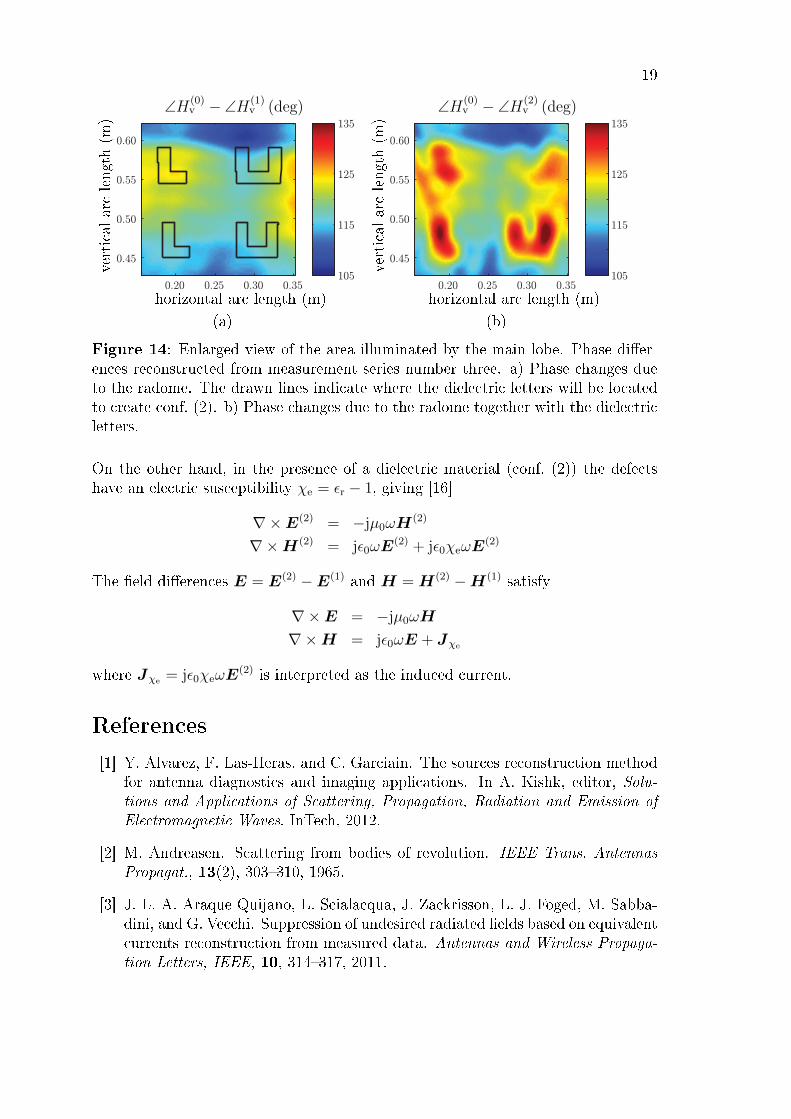
Figure 13: Enlarged view of the area illuminated by the main lobe. Phase di�er-ences reconstructed from measurement series number two. a) Phase changes due tothe radome. The drawn squares indicate where the dielectric patches will be locatedto create conf. (2). b) Phase changes due to the radome together with the dielectricsquares.
Acknowledgement
The measurements were carried out at GKN Aerospace Applied Composites' far-�eld facilities in Linköping, Sweden. Michael Andersson, GKN Aerospace AppliedComposites, Ljungby, Sweden, has been instrumental in questions regarding radomedevelopment, measurements and manufacturing. His help has been highly appreci-ated. We are also grateful to Christer Larsson at Saab Dynamics, Linköping, Swe-den, who did measurements on the relative permittivity of the dielectric tape. Theresearch reported in this paper is carried out under the auspices of FMV (Försvaretsmaterielverk) and their support is gratefully acknowledged.
Appendix A Induced currents due to dielectrics
A dielectric material introduces induced currents in the Maxwell equations. To seethis, start with the Maxwell equations for time harmonic �elds in a source freeregion (time convention ejωt),
∇×E = −jωB
∇×H = jωD
where E is the electric �eld, B is the magnetic �ux density, H is the magnetic�eld, and D is the electric �ux density, respectively. The constitutive relationsread D = ε0εrE and B = µ0µrH , where ε0 is the permittivity of free space, εr isthe relative permittivity, µ0 is the permeability of free space, and µr is the relativepermeability, respectively.
In the absence of defects, and outside the radome (conf. (1) in Figure 1) we have
∇×E(1) = −jµ0ωH(1)
∇×H(1) = jε0ωE(1)
19
0.20 0.25 0.30 0.35
0.45
0.50
0.55
0.60
105
115
125
135
(a)
horizontal arc length (m)
vertical
arclength(m
)∠H(0)
v − ∠H(1)v (deg)
0.20 0.25 0.30 0.35
0.45
0.50
0.55
0.60
105
115
125
135
(b)
horizontal arc length (m)
vertical
arclength(m
)
∠H(0)v − ∠H(2)
v (deg)
Figure 14: Enlarged view of the area illuminated by the main lobe. Phase di�er-ences reconstructed from measurement series number three. a) Phase changes dueto the radome. The drawn lines indicate where the dielectric letters will be locatedto create conf. (2). b) Phase changes due to the radome together with the dielectricletters.
On the other hand, in the presence of a dielectric material (conf. (2)) the defectshave an electric susceptibility χe = εr − 1, giving [16]
∇×E(2) = −jµ0ωH(2)
∇×H(2) = jε0ωE(2) + jε0χeωE
(2)
The �eld di�erences E = E(2) −E(1) and H = H(2) −H(1) satisfy
∇×E = −jµ0ωH
∇×H = jε0ωE + Jχe
where Jχe = jε0χeωE(2) is interpreted as the induced current.
References
[1] Y. Alvarez, F. Las-Heras, and C. Garciain. The sources reconstruction methodfor antenna diagnostics and imaging applications. In A. Kishk, editor, Solu-tions and Applications of Scattering, Propagation, Radiation and Emission ofElectromagnetic Waves. InTech, 2012.
[2] M. Andreasen. Scattering from bodies of revolution. IEEE Trans. AntennasPropagat., 13(2), 303�310, 1965.
[3] J. L. A. Araque Quijano, L. Scialacqua, J. Zackrisson, L. J. Foged, M. Sabba-dini, and G. Vecchi. Suppression of undesired radiated �elds based on equivalentcurrents reconstruction from measured data. Antennas and Wireless Propaga-tion Letters, IEEE, 10, 314�317, 2011.
20
−40
−35
−30
−25
−20
−15
−10
−5
0
(a)
|H(0)v |/max|H(0)
v | (dB)
50
70
90
110
130
150
(b)
∠H(0)v − ∠H(1)
v (deg)
Figure 15: Phase image of an earlier attempt to trim the radome. a) The illu-mination of the radome. The black lines indicate the location of the indentation.b) Phase change due to the radome.
[4] J. L. A. Araque Quijano and G. Vecchi. Field and source equivalence in sourcereconstruction on 3D surfaces. Progress In Electromagnetics Research, 103,67�100, 2010.
[5] A. Bondeson, T. Rylander, and P. Ingelström. Computational Electromagnetics.Springer-Verlag, Berlin, 2005.
[6] D. G. Burks. Radomes. In J. L. Volakis, editor, Antenna engineering handbook.pub-mcgraw, fourth edition, 2007.
[7] W. C. Chew, M. S. Tong, and B. Hu. Integral equation methods for electromag-netic and elastic waves, volume 12. Morgan & Claypool, 2008.
[8] D. Colton and R. Kress. Integral Equation Methods in Scattering Theory. JohnWiley & Sons, New York, 1983.
[9] T. F. Eibert, E. Kaliyaperumal, and C. H. Schmidt. Inverse equivalent surfacecurrent method with hierarchical higher order basis functions, full probe cor-rection and multilevel fast multipole acceleration. Progress In ElectromagneticsResearch, 106, 377�394, 2010.
[10] L. J. Foged, L. Scialacqua, F. Saccardi, J. L. Araque Quijano, G. Vecchi, andM. Sabbadini. Practical application of the equivalent source method as anantenna diagnostics tool. IEEE Antennas and Propagation Magazine, 54(5),243�249, 2012.
[11] E. Gimonet, A. Sarremejean, J. P. David, and P. Bossuet. Determination ofradome pertubation by inverse transform of radiation pattern. In Proc. of 5th
21
European Electromagnetic Windows Conference, pages 183�190, Juan-les-Pins,France, 1989.
[12] M. G. Guler and E. B. Joy. High resolution spherical microwave holography.IEEE Trans. Antennas Propagat., 43(5), 464�472, 1995.
[13] M. Gustafsson. Accurate and e�cient evaluation of modal Green's functions.Journal of Electromagnetic Waves and Applications, 24(10), 1291�1301, 2010.
[14] J. E. Hansen, editor. Spherical Near-Field Antenna Measurements. Number 26in IEE electromagnetic waves series. Peter Peregrinus Ltd., Stevenage, UK,1988. ISBN: 0-86341-110-X.
[15] P. C. Hansen. Discrete inverse problems: insight and algorithms, volume 7.Society for Industrial & Applied, 2010.
[16] J. D. Jackson. Classical Electrodynamics. John Wiley & Sons, New York, thirdedition, 1999.
[17] J. M. Jin. Theory and computation of electromagnetic �elds. Wiley OnlineLibrary, 2010.
[18] E. Jörgensen, D. W. Hess, P. Meincke, O. Borries, C. Cappellin, and J. Ford-ham. Antenna diagnostics on planar arrays using a 3D source reconstructiontechnique and spherical near-�eld measurements. In Antennas and Propagation(EUCAP), Proceedings of the 6th European Conference on, pages 2547�2550.IEEE, 2012.
[19] E. Jörgensen, P. Meincke, and C. Cappellin. Advanced processing of measured�elds using �eld reconstruction techniques. In Antennas and Propagation (EU-CAP), Proceedings of the 5th European Conference on, pages 3880�3884. IEEE,2011.
[20] D. J. Kozako�. Analysis of Radome-Enclosed Antennas. Artech House, Boston,London, 1997.
[21] R. Kress. Linear Integral Equations. Springer-Verlag, Berlin Heidelberg, secondedition, 1999.
[22] Y. A. Lopez, F. Las-Heras Andres, M. R. Pino, and T. K. Sarkar. An improvedsuper-resolution source reconstruction method. Instrumentation and Measure-ment, IEEE Transactions on, 58(11), 3855�3866, 2009.
[23] J. A. Lopez-Fernandez, M. Lopez-Portugues, Y. Alvarez Lopez, C. G. Gonzalez,D. Martínez, and F. Las-Heras. Fast antenna characterization using the sourcesreconstruction method on graphics processors. Progress In ElectromagneticsResearch, 126, 185�201, 2012.
[24] J. R. Mautz and R. F. Harrington. Radiation and scattering from bodies ofrevolution. Appl. Scienti�c Research, 20(1), 405�435, 1969.
22
[25] C. Müller. Foundations of the Mathematical Theory of Electromagnetic Waves.Springer-Verlag, Berlin, 1969.
[26] K. Persson, M. Gustafsson, and G. Kristensson. Reconstruction and visual-ization of equivalent currents on a radome using an integral representationformulation. Progress In Electromagnetics Research, 20, 65�90, 2010.
[27] K. Persson and M. Gustafsson. Reconstruction of equivalent currents using anear-�eld data transformation � with radome applications. Progress in Electro-magnetics Research, 54, 179�198, 2005.
[28] K. Persson and M. Gustafsson. Reconstruction of equivalent currents usingthe scalar surface integral representation. Technical Report LUTEDX/(TEAT-7131)/1�25/(2005), Lund University, Department of Electrical and In-formation Technology, P.O. Box 118, S-221 00 Lund, Sweden, 2005.http://www.eit.lth.se.
[29] Z. Shengfang, G. Dongming, K. Renke, J. Zhenyuan, S. Aifeng, and J. Tian. Re-search on microwave and millimeter-wave IPD measurement system for radome.In Microwave and Millimeter Wave Technology, 2004. ICMMT 4th Interna-tional Conference on, Proceedings, pages 711�714. IEEE, 2004.
[30] S. Ström. Introduction to integral representations and integral equations fortime-harmonic acoustic, electromagnetic and elastodynamic wave �elds. InV. V. Varadan, A. Lakhtakia, and V. K. Varadan, editors, Field Representationsand Introduction to Scattering, volume 1 of Handbook on Acoustic, Electromag-netic and Elastic Wave Scattering, chapter 2, pages 37�141. Elsevier SciencePublishers, Amsterdam, 1991.
[31] A. B. Strong. Fundamentals of composites manufacturing: materials, methodsand applications. Society of Manufacturing Engineers, 2008.
[32] J. G. Van Bladel. Electromagnetic Fields. IEEE Press, Piscataway, NJ, secondedition, 2007.
[33] B. Widenberg. Advanced compact test range for both radome and antennameasurement. In 11th European Electromagnetic Structures Conference, pages183�186, Torino, Italy, 2005.
[34] A. D. Yaghjian. An overview of near-�eld antenna measurements. IEEE Trans.Antennas Propagat., 34(1), 30�45, January 1986.