annex section - archived web sites - institute for environment...
TRANSCRIPT

ANNEX SECTION
ANNEX 1
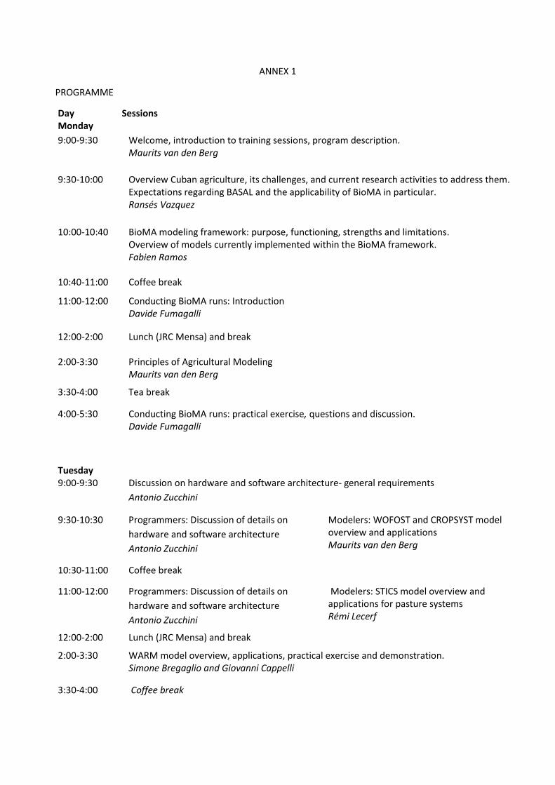
PROGRAMME
Day Sessions Monday
9:00-9:30 Welcome, introduction to training sessions, program description. Maurits van den Berg
9:30-10:00 Overview Cuban agriculture, its challenges, and current research activities to address them. Expectations regarding BASAL and the applicability of BioMA in particular. Ransés Vazquez
10:00-10:40 BioMA modeling framework: purpose, functioning, strengths and limitations. Overview of models currently implemented within the BioMA framework. Fabien Ramos
10:40-11:00 Coffee break
11:00-12:00 Conducting BioMA runs: Introduction Davide Fumagalli
12:00-2:00 Lunch (JRC Mensa) and break
2:00-3:30 Principles of Agricultural Modeling Maurits van den Berg
3:30-4:00 Tea break
4:00-5:30 Conducting BioMA runs: practical exercise, questions and discussion. Davide Fumagalli
Tuesday 9:00-9:30 Discussion on hardware and software architecture- general requirements
Antonio Zucchini
9:30-10:30 Programmers: Discussion of details on
hardware and software architecture
Antonio Zucchini
Modelers: WOFOST and CROPSYST model overview and applications Maurits van den Berg
10:30-11:00 Coffee break
11:00-12:00 Programmers: Discussion of details on
hardware and software architecture
Antonio Zucchini
Modelers: STICS model overview and applications for pasture systems Rémi Lecerf
12:00-2:00 Lunch (JRC Mensa) and break
2:00-3:30 WARM model overview, applications, practical exercise and demonstration. Simone Bregaglio and Giovanni Cappelli
3:30-4:00 Coffee break

4:00-5:30 WARM model continuation Simone Bregaglio and Giovanni Cappelli
Wednesday
9:00-10:30 Develop BioMA modeling solutions - Introduction to Bioma model layer - Step by step training for the creation of a model layer modeling solution (exercise 1) Davide Fumagalli
10:30-11:00 Coffee break
11:00-11:50 Exercise 1 continuation
12:00-1:30 Lunch (JRC Mensa) and break
1:40-2:50 Optimizer component, Davide Fanchini
2:50-3:30 Discussion session: Data requirements, availability and procurement strategies - Weather - Soils - Crop parameters - Agro-management All BASAL team, moderated by Joysee Rodriguez
3:30-4:00 Tea/coffee break
4:00-5:30 Discussion session on data requirements, continuation
Thursday 9:00-10:30 Develop BioMA modeling solutions
- Independent work for the creation of a model layer modeling solution (exercise 2) Davide Fumagalli
10:30-11:00 Coffee break
11:00-11:50 Exercise 2 continuation
12:00-1:30 Lunch (JRC Mensa) and break
1:40-3:30 Develop BioMA modeling solutions - Introduction to Bioma composition layer - Step by step training for the creation of a composition layer modeling solution (exercise 3) - Independent work for the creation of a composition layer modeling solution (exercise 4) Davide Fumagalli
3:30-4:00 Coffee break 4:30-5:20 Exercise 4 continuation

Friday 9:00-10:30 Develop BioMA modeling solutions
- Introduction to exercise 5: Introduction to Bioma configuration layer - Step by step guide for the creation of a configuration layer modeling solution (exercise 5) Davide Fumagalli
10:30-11:00 Coffee break
11:00-12:00 Continuation exercise 5
12:00-1:30 Lunch (JRC Mensa)
1:30-2:20 Preparation of presentations on exercises participants
2:20-3:30 Presentations from participants
3:31-4:00 Tea/coffee break
4:01-5:30 - Any remaining matters - Final discussion; Expectations revisited Evaluation of training course
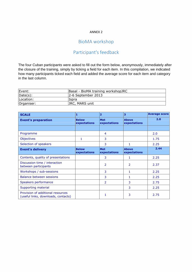
ANNEX 2
BioMA workshop
Participant's feedback
The four Cuban participants were asked to fill out the form below, anonymously, immediately after
the closure of the training, simply by ticking a field for each item. In this compilation, we indicated
how many participants ticked each field and added the average score for each item and category
in the last column.
Event: Basal - BioMA training workshopJRC
Date(s): 2-6 September 2013
Location: Ispra
Organiser: JRC, MARS unit
SCALE 1 2 3 Average score
Event's preparation Below expectations
Met expectations
Above expectations
2.0
Programme 4 2.0
Objectives 1 3 1.75
Selection of speakers 3 1 2.25
Event's delivery Below
expectations
Met
expectations
Above
expectations
2.44
Contents, quality of presentations 3 1 2.25
Discussion time / interaction
between participants 2 2 2.37
Workshops / sub-sessions 3 1 2.25
Balance between sessions 3 1 2.25
Speakers performance 2 3 2.75
Supporting material 3 2.25
Provision of additional resources
(useful links, downloads, contacts) 1 3 2.75

SCALE 1 2 3 Average
Organisation and Logistics Below expectations
Met expectations
Above expectations
3.0
Organisation, communication with
the participants 4 3.0
Meeting venue 4 3.0
Transport from airport to hotel 4 3.0
Hotel 2 2 2.5
Transport from hotel to venue 4 3.0
Lunches 4 3.25
Welcome dinner 4 3.25
Content Below expectations
Met expectations
Above expectations
2.56
Capacity of the training to meet
your learning objectives and its relevance for your work
2 2 2.12
Quality and accuracy of contents 3 3.0
Methodology Below
expectations
Met
expectations
Above
expectations
2.43
Length of the course and balance
between theory and practice 1 3 1.87
Possibility of interaction with trainer
and other participants 4 3.0
Learning Resources (Manuals,
Presentation Material, Hand-outs, etc)
Below
expectations
Met
expectations
Above
expectations
2.62
Usefulness and usability of course
material/presentations 2 2 2.5
Provision of additional resources (useful links, downloads, contacts)
1 3 2.75
Trainer / Facilitator Below expectations
Met expectations
Above expectations
2.87
Trainer's communication and interaction
3 1 2.75
Trainer's knowledge of the topic 4 3.0
General Comments Below expectations
Met expectations
Above expectations
Overall evaluation of the event 1 3 2.75
Any additional comment (especially for explaining the reasons for “below expectations")
Direct quotes from participants written comments:
The BioMA platform is fantastic in design, very tunable, but this implies that the time was not enough to comprehend and assimilate everything. We had no time to write down the full experience speakers
transmitted us at every step. [the software] is very complicated in itself and we needed more time to repeat each practice. We also need a procedure specific guide of each of the processes reviewed. Orally expressed comments:
I liked the training, and now we understand better BioMA and how to use the tools for modifying it, but we are not agronomist, so we need others to give us the procedures, or

components that will be added. For initiate learning in modifying
it we need more exercises like the ones studied here to practice adding new strategies or components. With our programming skills we can easily code any strategies but we need some more exercises to fully learn the steps in BioMA framework. We could do it independently if we have a good guide, and additional exercises.
There are too many steps involved in setting each model run, and I am not sure I will be able to remember all the necessary steps. We need a more specified guide that provides step by step each of the process either for running a ready model solution or for developing a new one. It could be even better if
the guides are developed with the ready initial tool for Cuba and maybe even in Spanish. More training will be needed and it could be great if the Davide Fumagalli could also be in the training in Cuba since his years of
experience with allow for fast clarification on technical problems and issues that often come when experimenting with modifying
previous versions. Maybe we needed more time for really assimilating the tool to a level that will be necessary to train others in our Institute.

ANNEX 3
List of Participants and Contributors
Name Contact Information
Instituto de Metereologia-Cuba INSMET
Roger Rolando Rivero Jaspe [email protected]
Ransés José Vázquez Montenegro Ransé[email protected] Ransé[email protected]
Malena Silva Lorenzo [email protected]
Frank Ernesto Pérez Acuña [email protected]
Joint Research Center
Maurits Van den Berg [email protected]
Stefan Niemeyer [email protected]
Davide Fumagalli [email protected]
Antonio Zucchini [email protected]
Fabien Ramos [email protected]
Davide Fanchini [email protected]
Rémi Lecerf [email protected]
Joysee Rodriguez Baide [email protected]
Beatriz Vidal-Legaz [email protected]
Ezio Crestaz [email protected]
University of Milano
Simone Ugo Bregaglio [email protected]
Giovanni Cappelli [email protected]
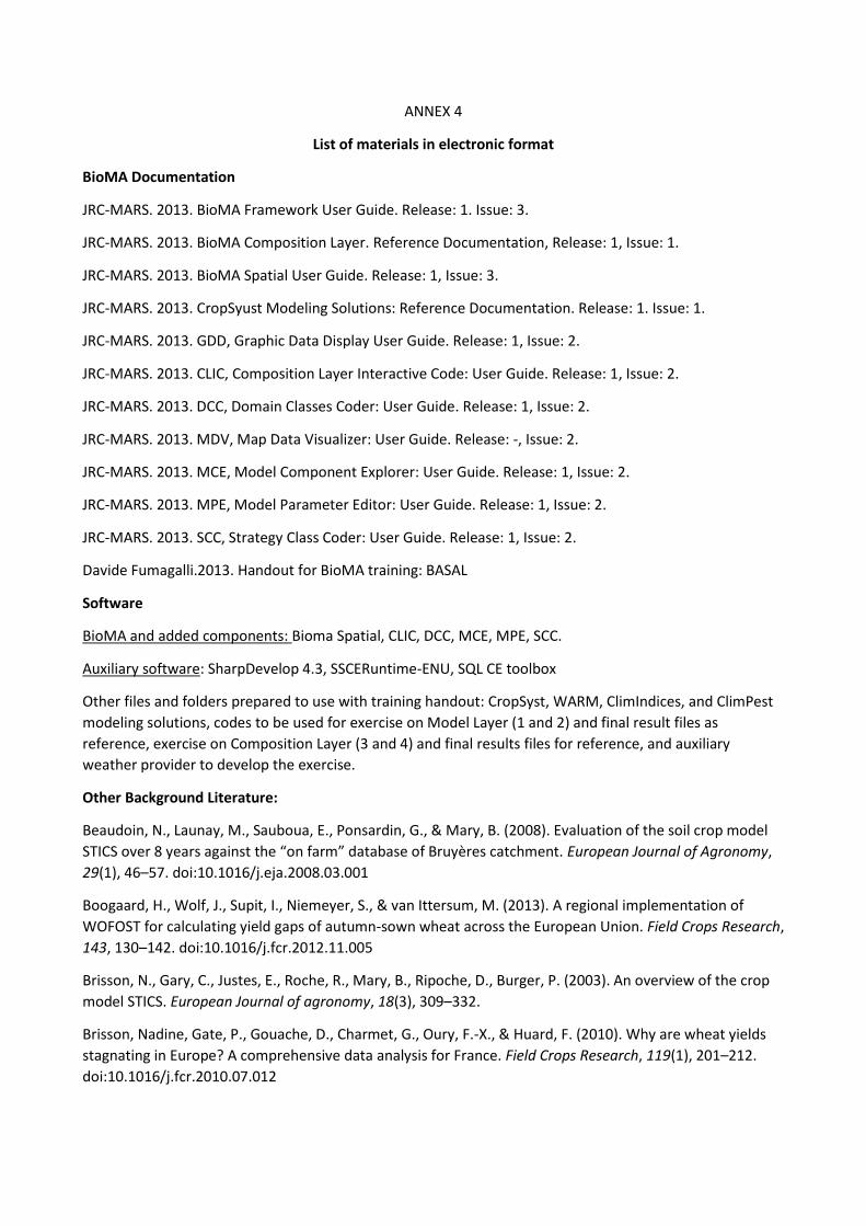
ANNEX 4
List of materials in electronic format
BioMA Documentation
JRC-MARS. 2013. BioMA Framework User Guide. Release: 1. Issue: 3.
JRC-MARS. 2013. BioMA Composition Layer. Reference Documentation, Release: 1, Issue: 1.
JRC-MARS. 2013. BioMA Spatial User Guide. Release: 1, Issue: 3.
JRC-MARS. 2013. CropSyust Modeling Solutions: Reference Documentation. Release: 1. Issue: 1.
JRC-MARS. 2013. GDD, Graphic Data Display User Guide. Release: 1, Issue: 2.
JRC-MARS. 2013. CLIC, Composition Layer Interactive Code: User Guide. Release: 1, Issue: 2.
JRC-MARS. 2013. DCC, Domain Classes Coder: User Guide. Release: 1, Issue: 2.
JRC-MARS. 2013. MDV, Map Data Visualizer: User Guide. Release: -, Issue: 2.
JRC-MARS. 2013. MCE, Model Component Explorer: User Guide. Release: 1, Issue: 2.
JRC-MARS. 2013. MPE, Model Parameter Editor: User Guide. Release: 1, Issue: 2.
JRC-MARS. 2013. SCC, Strategy Class Coder: User Guide. Release: 1, Issue: 2.
Davide Fumagalli.2013. Handout for BioMA training: BASAL
Software
BioMA and added components: Bioma Spatial, CLIC, DCC, MCE, MPE, SCC.
Auxiliary software: SharpDevelop 4.3, SSCERuntime-ENU, SQL CE toolbox
Other files and folders prepared to use with training handout: CropSyst, WARM, ClimIndices, and ClimPest
modeling solutions, codes to be used for exercise on Model Layer (1 and 2) and final result files as
reference, exercise on Composition Layer (3 and 4) and final results files for reference, and auxiliary
weather provider to develop the exercise.
Other Background Literature:
Beaudoin, N., Launay, M., Sauboua, E., Ponsardin, G., & Mary, B. (2008). Evaluation of the soil crop model
STICS over 8 years against the “on farm” database of Bruyères catchment. European Journal of Agronomy,
29(1), 46–57. doi:10.1016/j.eja.2008.03.001
Boogaard, H., Wolf, J., Supit, I., Niemeyer, S., & van Ittersum, M. (2013). A regional implementation of
WOFOST for calculating yield gaps of autumn-sown wheat across the European Union. Field Crops Research,
143, 130–142. doi:10.1016/j.fcr.2012.11.005
Brisson, N., Gary, C., Justes, E., Roche, R., Mary, B., Ripoche, D., Burger, P. (2003). An overview of the crop
model STICS. European Journal of agronomy, 18(3), 309–332.
Brisson, Nadine, Gate, P., Gouache, D., Charmet, G., Oury, F.-X., & Huard, F. (2010). Why are wheat yields
stagnating in Europe? A comprehensive data analysis for France. Field Crops Research, 119(1), 201–212.
doi:10.1016/j.fcr.2010.07.012

Caubel, J., Launay, M., Lannou, C., & Brisson, N. (2012). Generic response functions to simulate climate-
based processes in models for the development of airborne fungal crop pathogens. Ecological Modelling,
242, 92–104. doi:10.1016/j.ecolmodel.2012.05.012
Confalonieri, R., Bregaglio, S., Donatelli, M., Tubiello, F., & Fernandes, E. (2012). Agroecological Zones
Simulator (AZS): A component based, open-access, transparent platform for climate change–crop
productivity impact assessment in Latin America. Retrieved from
http://www.iemss.org/iemss2012/proceedings/C3_0915_Confalonieri_et_al.pdf
Confalonieri, R., Donatelli, M., Bregaglio, S., Stella, T., Negrini, G., & Donatelli, M. (2012a). An extensible,
multi-model software library for simulating crop growth and development. In International Environmental
Modelling and Software Society (iEMSs) 6th International Congress, Leipzig, Germany. Retrieved from
http://www.iemss.org/sites/iemss2012/proceedings/C3_0836_Confalonieri_et_al.pdf
Confalonieri, R., Donatelli, M., Bregaglio, S., Stella, T., Negrini, G., & Donatelli, M. (2012b). An extensible,
multi-model software library for simulating crop growth and development. In International Environmental
Modelling and Software Society (iEMSs) 6th International Congress, Leipzig, Germany. Retrieved from
http://www.iemss.org/sites/iemss2012/proceedings/C3_0836_Confalonieri_et_al.pdf
Confalonieri, Roberto, Acutis, M., Bellocchi, G., & Donatelli, M. (2009). Multi-metric evaluation of the
models WARM, CropSyst, and WOFOST for rice. Ecological Modelling, 220(11), 1395–1410.
doi:10.1016/j.ecolmodel.2009.02.017
Confalonieri, Roberto, Bellocchi, G., Tarantola, S., Acutis, M., Donatelli, M., & Genovese, G. (2010).
Sensitivity analysis of the rice model WARM in Europe: Exploring the effects of different locations, climates
and methods of analysis on model sensitivity to crop parameters. Environmental Modelling & Software,
25(4), 479–488. doi:10.1016/j.envsoft.2009.10.005
Confalonieri, Roberto, Bregaglio, S., Rosenmund, A. S., Acutis, M., & Savin, I. (2011). A model for simulating
the height of rice plants. European Journal of Agronomy, 34(1), 20–25. doi:10.1016/j.eja.2010.09.003
Confalonieri, Roberto, Rosenmund, A. S., & Baruth, B. (2009). An improved model to simulate rice yield.
Agronomy for Sustainable Development, 29(3), 463–474. doi:10.1051/agro/2009005
Constantin, J., Beaudoin, N., Launay, M., Duval, J., & Mary, B. (2012). Long-term nitrogen dynamics in
various catch crop scenarios: Test and simulations with STICS model in a temperate climate. Agriculture,
Ecosystems & Environment, 147, 36–46. doi:10.1016/j.agee.2011.06.006
Corre-Hellou, G., Faure, M., Launay, M., Brisson, N., & Crozat, Y. (2009). Adaptation of the STICS intercrop
model to simulate crop growth and N accumulation in pea–barley intercrops. Field Crops Research, 113(1),
72–81. doi:10.1016/j.fcr.2009.04.007
Díaz-Ambrona, C. G. H., O’Leary, G. J., Sadras, V. O., O’Connell, M. G., & Connor, D. J. (2005). Environmental
risk analysis of farming systems in a semi-arid environment: effect of rotations and management practices
on deep drainage. Field Crops Research, 94(2-3), 257–271. doi:10.1016/j.fcr.2005.01.008
Jalota, S. K., Singh, S., Chahal, G. B. S., Ray, S. S., Panigraghy, S., Bhupinder-Singh, & Singh, K. B. (2010). Soil
texture, climate and management effects on plant growth, grain yield and water use by rainfed maize–
wheat cropping system: Field and simulation study. Agricultural Water Management, 97(1), 83–90.
doi:10.1016/j.agwat.2009.08.012
Jégo, G., Martínez, M., Antigüedad, I., Launay, M., Sanchez-Pérez, J. M., & Justes, E. (2008). Evaluation of
the impact of various agricultural practices on nitrate leaching under the root zone of potato and sugar
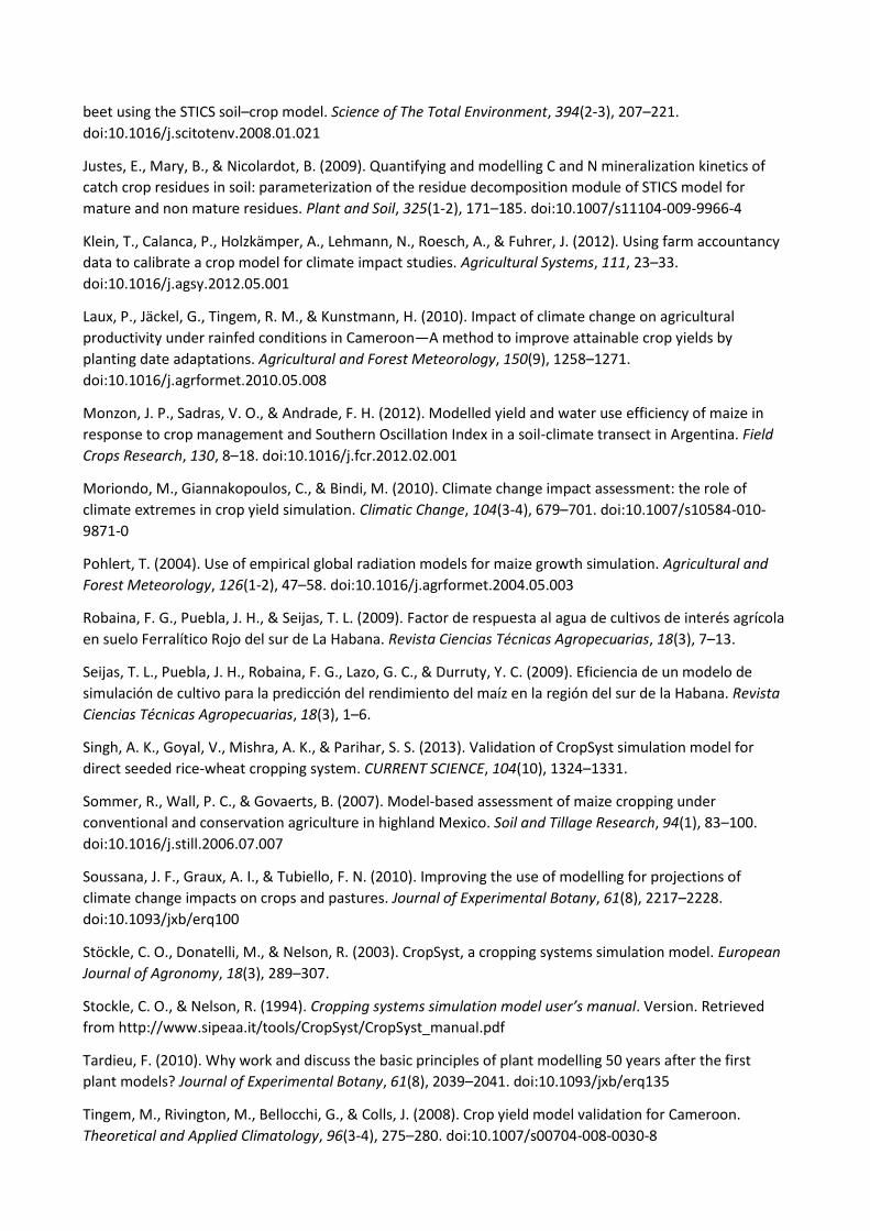
beet using the STICS soil–crop model. Science of The Total Environment, 394(2-3), 207–221.
doi:10.1016/j.scitotenv.2008.01.021
Justes, E., Mary, B., & Nicolardot, B. (2009). Quantifying and modelling C and N mineralization kinetics of
catch crop residues in soil: parameterization of the residue decomposition module of STICS model for
mature and non mature residues. Plant and Soil, 325(1-2), 171–185. doi:10.1007/s11104-009-9966-4
Klein, T., Calanca, P., Holzkämper, A., Lehmann, N., Roesch, A., & Fuhrer, J. (2012). Using farm accountancy
data to calibrate a crop model for climate impact studies. Agricultural Systems, 111, 23–33.
doi:10.1016/j.agsy.2012.05.001
Laux, P., Jäckel, G., Tingem, R. M., & Kunstmann, H. (2010). Impact of climate change on agricultural
productivity under rainfed conditions in Cameroon—A method to improve attainable crop yields by
planting date adaptations. Agricultural and Forest Meteorology, 150(9), 1258–1271.
doi:10.1016/j.agrformet.2010.05.008
Monzon, J. P., Sadras, V. O., & Andrade, F. H. (2012). Modelled yield and water use efficiency of maize in
response to crop management and Southern Oscillation Index in a soil-climate transect in Argentina. Field
Crops Research, 130, 8–18. doi:10.1016/j.fcr.2012.02.001
Moriondo, M., Giannakopoulos, C., & Bindi, M. (2010). Climate change impact assessment: the role of
climate extremes in crop yield simulation. Climatic Change, 104(3-4), 679–701. doi:10.1007/s10584-010-
9871-0
Pohlert, T. (2004). Use of empirical global radiation models for maize growth simulation. Agricultural and
Forest Meteorology, 126(1-2), 47–58. doi:10.1016/j.agrformet.2004.05.003
Robaina, F. G., Puebla, J. H., & Seijas, T. L. (2009). Factor de respuesta al agua de cultivos de interés agrícola
en suelo Ferralítico Rojo del sur de La Habana. Revista Ciencias Técnicas Agropecuarias, 18(3), 7–13.
Seijas, T. L., Puebla, J. H., Robaina, F. G., Lazo, G. C., & Durruty, Y. C. (2009). Eficiencia de un modelo de
simulación de cultivo para la predicción del rendimiento del maíz en la región del sur de la Habana. Revista
Ciencias Técnicas Agropecuarias, 18(3), 1–6.
Singh, A. K., Goyal, V., Mishra, A. K., & Parihar, S. S. (2013). Validation of CropSyst simulation model for
direct seeded rice-wheat cropping system. CURRENT SCIENCE, 104(10), 1324–1331.
Sommer, R., Wall, P. C., & Govaerts, B. (2007). Model-based assessment of maize cropping under
conventional and conservation agriculture in highland Mexico. Soil and Tillage Research, 94(1), 83–100.
doi:10.1016/j.still.2006.07.007
Soussana, J. F., Graux, A. I., & Tubiello, F. N. (2010). Improving the use of modelling for projections of
climate change impacts on crops and pastures. Journal of Experimental Botany, 61(8), 2217–2228.
doi:10.1093/jxb/erq100
Stöckle, C. O., Donatelli, M., & Nelson, R. (2003). CropSyst, a cropping systems simulation model. European
Journal of Agronomy, 18(3), 289–307.
Stockle, C. O., & Nelson, R. (1994). Cropping systems simulation model user’s manual. Version. Retrieved
from http://www.sipeaa.it/tools/CropSyst/CropSyst_manual.pdf
Tardieu, F. (2010). Why work and discuss the basic principles of plant modelling 50 years after the first
plant models? Journal of Experimental Botany, 61(8), 2039–2041. doi:10.1093/jxb/erq135
Tingem, M., Rivington, M., Bellocchi, G., & Colls, J. (2008). Crop yield model validation for Cameroon.
Theoretical and Applied Climatology, 96(3-4), 275–280. doi:10.1007/s00704-008-0030-8

Tingem, M., Rivington, M., & Colls, J. (2008). Climate variability and maize production in Cameroon:
Simulating the effects of extreme dry and wet years. Singapore Journal of Tropical Geography, 29(3), 357–
370. doi:10.1111/j.1467-9493.2008.00344.x
Van Ittersum, M. K., Leffelaar, P. A., Van Keulen, H., Kropff, M. J., Bastiaans, L., & Goudriaan, J. (2003). On
approaches and applications of the Wageningen crop models. European Journal of Agronomy, 18(3), 201–
234.
Van Ittersum, M. K., & Rabbinge, R. (1997). Concepts in production ecology for analysis and quantification
of agricultural input-output combinations. Field Crops Research, 52(3), 197–208.
Wang, T., Lu, C., & Yu, B. (2011). Production potential and yield gaps of summer maize in the Beijing-Tianjin-
Hebei Region. Journal of Geographical Sciences, 21(4), 677–688. doi:10.1007/s11442-011-0872-3
White, J. W., Hoogenboom, G., Kimball, B. A., & Wall, G. W. (2011a). Methodologies for simulating impacts
of climate change on crop production. Field Crops Research, 124(3), 357–368. doi:10.1016/j.fcr.2011.07.001
White, J. W., Hoogenboom, G., Kimball, B. A., & Wall, G. W. (2011b). Methodologies for simulating impacts
of climate change on crop production. Field Crops Research, 124(3), 357–368. doi:10.1016/j.fcr.2011.07.001

ANNEX 5
Presentations slides
10/25/2013
1
BioMA framework introduction - Training of Ms. Emilija Poposka
Jan 21, 2013, JRC, Ispra, Italy
The BioMA framework
Davide Fumagalli
On behalf of the Development Team
Institute for Environment and Sustainability
Joint Research Centre
1
BioMA framework introduction - Training of Ms. Emilija Poposka
Jan 21, 2013, JRC, Ispra, Italy
Why BioMA framework
High level requirements:
• To increase the trasparency of the modelling solutions being built
compared to legacy code available, for each of the modelling solutions
being built;
• To increase the traceability of performance of each modelling unit used
in modelling solutions;
• To involve teams other than JRC without requiring them to commit to
a whole infrastructure they would not own and possibly would not use.
Summary: to maximize both reusability and openness
we chose to develop a simulation system based on framework-
indipendent components, both for model and for tool components.
2
10/25/2013
2
BioMA framework introduction - Training of Ms. Emilija Poposka
Jan 21, 2013, JRC, Ispra, Italy
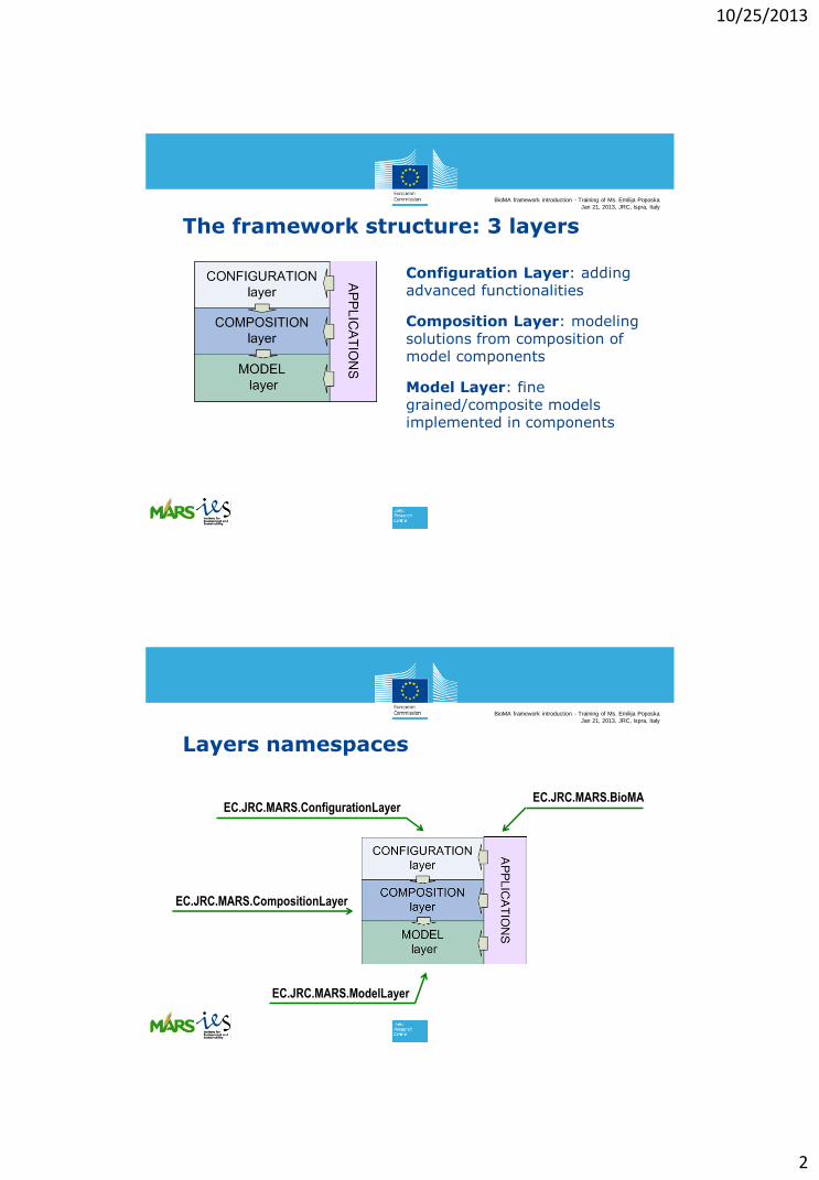
The framework structure: 3 layers
Configuration Layer: adding advanced functionalities
Composition Layer: modeling solutions from composition of model components
Model Layer: fine grained/composite models implemented in components
BioMA framework introduction - Training of Ms. Emilija Poposka
Jan 21, 2013, JRC, Ispra, Italy
EC.JRC.MARS.ConfigurationLayer
EC.JRC.MARS.CompositionLayer
EC.JRC.MARS.ModelLayer
EC.JRC.MARS.BioMA
Layers namespaces

10/25/2013
3
BioMA framework introduction - Training of Ms. Emilija Poposka
Jan 21, 2013, JRC, Ispra, Italy
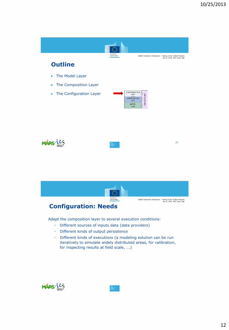
Outline
● The Model Layer
● The Composition Layer
● The Configuration Layer
5
BioMA framework introduction - Training of Ms. Emilija Poposka
Jan 21, 2013, JRC, Ispra, Italy
The Model layer (1)
6
• Set of classes to
code model/process
algorithms
(Strategies)

10/25/2013
4
BioMA framework introduction - Training of Ms. Emilija Poposka
Jan 21, 2013, JRC, Ispra, Italy
The Model layer (2)
Each model is implemented as a strategy class which:
• Contains the algorithm/equation of the model
• Contains the definition of its own parameters
• Implements the test of pre- and post-conditions (inputs/params/outputs
validation)
• May use other classes (strategies) sharing the same interface
• Implements a scalable logging system
• Exposes the list of its inputs, outputs, simulation options, and parameters
• Exposes instances of concepts defined in a reference ontology
7
BioMA framework introduction - Training of Ms. Emilija Poposka
Jan 21, 2013, JRC, Ispra, Italy
The Model layer (3)
Each variable used by the models (input, output or parameter) is
represented by a set of properties detailing a description,
max/min/default values, units, value type. (VarInfo class)
Each set of related variables is contained in a domain class which
represents a state of the simulated process (e.g. State of a plant)
All the strategies of the same library (component) share the same
domain classes, since the models share the same simulated physical
domain
8

10/25/2013
5
BioMA framework introduction - Training of Ms. Emilija Poposka
Jan 21, 2013, JRC, Ispra, Italy
The Model layer (4)
Models are implemented using structural and behavioral design patterns
which foster extensibility and reusability:
• Composite (facilitating the use of composite and simple strategies)
• Strategy (allowing a context specific selection of models at run-time)
• Bridge (allowing the replacement of model components)
Models are made available with model and code documentation, and with sample projects for component reuse and extension.
9
BioMA framework introduction - Training of Ms. Emilija Poposka
Jan 21, 2013, JRC, Ispra, Italy
Model layer tools
Applications are provided to:
• Explore component interfaces and domain classes: Model Component Explorer
• Generate the code of domain classes and parameter classes: Domain Class Coder
• Generate the code of model classes (strategies): Strategy Class Coder
• View/edit the values of the models parameters: Model Parameter Editor
10

10/25/2013
6
BioMA framework introduction - Training of Ms. Emilija Poposka
Jan 21, 2013, JRC, Ispra, Italy
The BioMA model layer libraries:
11
BioMA framework introduction - Training of Ms. Emilija Poposka
Jan 21, 2013, JRC, Ispra, Italy
Outline
● The Model Layer
● The Composition Layer
● The Configuration Layer
12
10/25/2013
7
BioMA framework introduction - Training of Ms. Emilija Poposka
Jan 21, 2013, JRC, Ispra, Italy
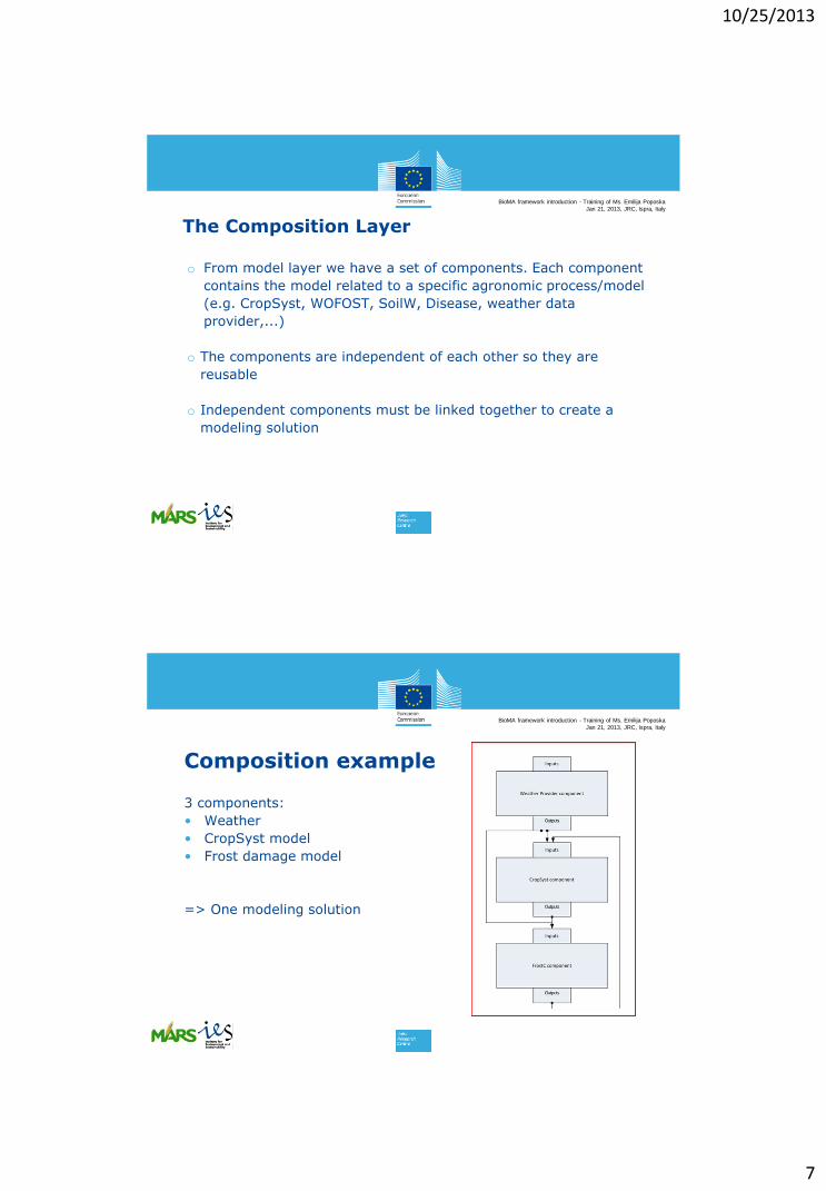
The Composition Layer
o From model layer we have a set of components. Each component
contains the model related to a specific agronomic process/model
(e.g. CropSyst, WOFOST, SoilW, Disease, weather data
provider,...)
o The components are independent of each other so they are
reusable
o Independent components must be linked together to create a
modeling solution
BioMA framework introduction - Training of Ms. Emilija Poposka
Jan 21, 2013, JRC, Ispra, Italy
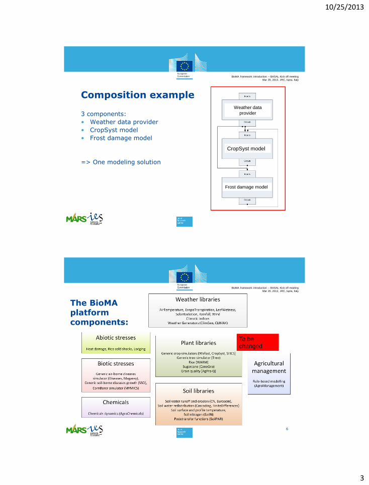
Composition example
3 components:
• Weather
• CropSyst model
• Frost damage model
=> One modeling solution

10/25/2013
8
BioMA framework introduction - Training of Ms. Emilija Poposka
Jan 21, 2013, JRC, Ispra, Italy
Composition Layer purposes
• To define a cycle of simulation.
• Definition of the calling order of the components
• Calls at the time step chosen for communication across components
in the modeling solution (e.g. daily time steps or hourly time steps,
depending on the models)
To handle events to manage actions which are triggered not at
all time steps (e.g. agro-management events).
• To collect the models outputs into an aggregated model
output
• To return the aggregated output of the modeling solution (in
principle excluding persistence, which is part of the configuration,
hence context specific).
15
BioMA framework introduction - Training of Ms. Emilija Poposka
Jan 21, 2013, JRC, Ispra, Italy
Composition Layer purposes (2)
o To provide to the higher level (Configuration level, Application)
aggregated informations (e.g. Modeling solution’s
inputs/ouputs/parameters/metadata)
o To provide to the higher level info about the components
used and how they are linked togheter
o To allow transfer of modeling options from the higher level
10/25/2013
9
BioMA framework introduction - Training of Ms. Emilija Poposka
Jan 21, 2013, JRC, Ispra, Italy
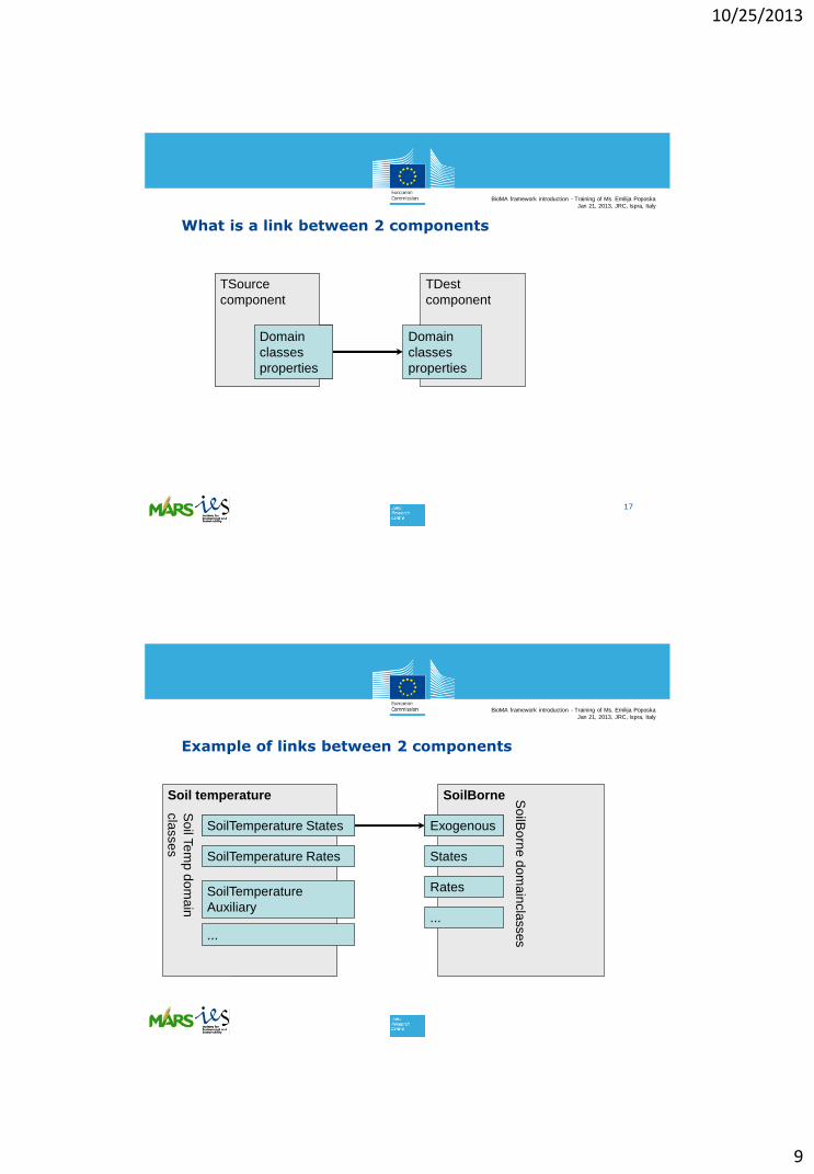
What is a link between 2 components
17
TSource
component
Domain
classes
properties
TSource
component
Domain
classes
properties
TDest
component
Domain
classes
properties
BioMA framework introduction - Training of Ms. Emilija Poposka
Jan 21, 2013, JRC, Ispra, Italy
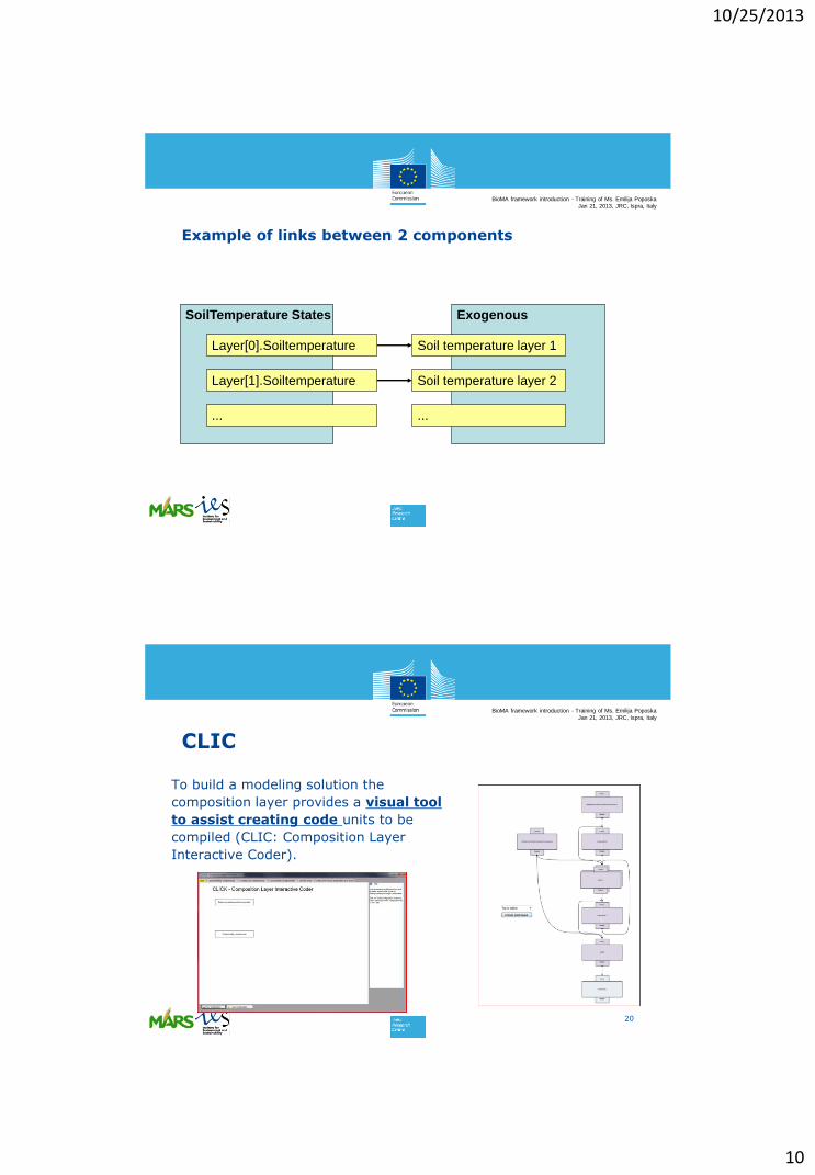
Example of links between 2 components
TSource
component
Soil temperature
SoilTemperature States
SoilBorne
Exogenous
SoilTemperature Rates
SoilTemperature
Auxiliary
States
Rates
...
...
So
ilBo
rne
do
ma
incla
sses
So
il Te
mp
do
ma
in
cla
sse
s
SoilTemperature States Exogenous
10/25/2013
10
BioMA framework introduction - Training of Ms. Emilija Poposka
Jan 21, 2013, JRC, Ispra, Italy
Example of links between 2 components
SoilTemperature States Exogenous
Soil temperature layer 1
Soil temperature layer 2
Layer[0].Soiltemperature
Layer[1].Soiltemperature
... ...
BioMA framework introduction - Training of Ms. Emilija Poposka
Jan 21, 2013, JRC, Ispra, Italy
CLIC
To build a modeling solution the
composition layer provides a visual tool
to assist creating code units to be
compiled (CLIC: Composition Layer
Interactive Coder).
20

10/25/2013
11
BioMA framework introduction - Training of Ms. Emilija Poposka
Jan 21, 2013, JRC, Ispra, Italy
The sample modeling solution (CropSyst)
Agronomic components:
CropSyst Potential
CropSyst Water Limited
Soil Water content
Soil Runoff Erosion
Soil Temperature
SoilBorne
Auxiliary components:
Weather data provider
Soil data provider
Agromanagement
BioMA framework introduction - Training of Ms. Emilija Poposka
Jan 21, 2013, JRC, Ispra, Italy
Soil Borne
Weather
CropSyst
potential
SoilWater
content
Soil temperature
Soil dataAgromanagement
CropSyst Water
Limited
Soil runoff erosion
10/25/2013
12
BioMA framework introduction - Training of Ms. Emilija Poposka
Jan 21, 2013, JRC, Ispra, Italy
Outline
● The Model Layer
● The Composition Layer
● The Configuration Layer
23
BioMA framework introduction - Training of Ms. Emilija Poposka
Jan 21, 2013, JRC, Ispra, Italy
Configuration: Needs
Adapt the composition layer to several execution conditions:
• Different sources of inputs data (data providers)
• Different kinds of output persistence
• Different kinds of executions (a modeling solution can be run
iteratively to simulate widely distributed areas, for calibration,
for inspecting results at field scale, ...)
10/25/2013
13
BioMA framework introduction - Training of Ms. Emilija Poposka
Jan 21, 2013, JRC, Ispra, Italy
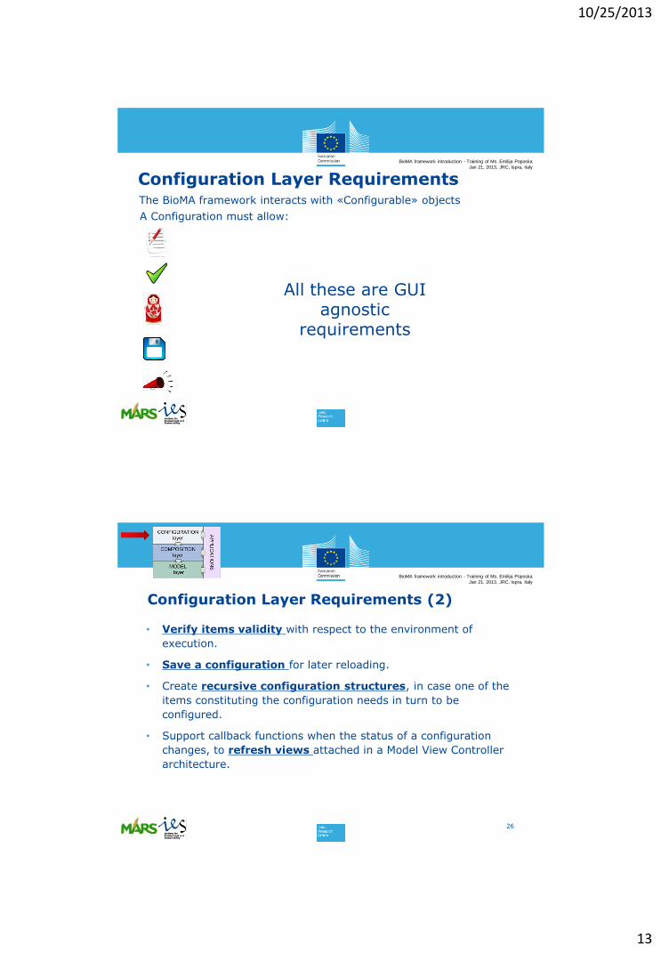
Configuration Layer RequirementsThe BioMA framework interacts with «Configurable» objects
A Configuration must allow:
To be validated
To be saved and reloaded later
To notify changes in its status (MVC applications)
To be composed in complex configurations
To be defined in terms of items to fill
All
All these are GUIagnostic
requirements
BioMA framework introduction - Training of Ms. Emilija Poposka
Jan 21, 2013, JRC, Ispra, Italy
Configuration Layer Requirements (2)
• Verify items validity with respect to the environment of
execution.
• Save a configuration for later reloading.
• Create recursive configuration structures, in case one of the
items constituting the configuration needs in turn to be
configured.
• Support callback functions when the status of a configuration
changes, to refresh views attached in a Model View Controller
architecture.
26

10/25/2013
14
BioMA framework introduction - Training of Ms. Emilija Poposka
Jan 21, 2013, JRC, Ispra, Italy
BioMA applications summary
2 phases:
1. Modeling solution development:
A modeler/programmer creates a modeling solution starting from model
layer by using: SCC, DCC, and other model layer tools
The modeler/programmer creates the composition/configuration layer
by using CLIC application
2. Modeling solution use:
The modeler loads the modeling solution into BioMA Spatial or BioMA
Point, and run it
The modeler loads the modeling solution into Optimizer or LUISA to
perform a parameters calibration or a sensitivity analysis
27
BioMA framework introduction - Training of Ms. Emilija Poposka
Jan 21, 2013, JRC, Ispra, Italy
BioMA Point
• To run a modeling solution on a specific location/time interval
with an high level of detail on the modeling solution’s
components.
• Used mainly for the first tests of the modeling solution.
28
10/25/2013
15
BioMA framework introduction - Training of Ms. Emilija Poposka
Jan 21, 2013, JRC, Ispra, Italy
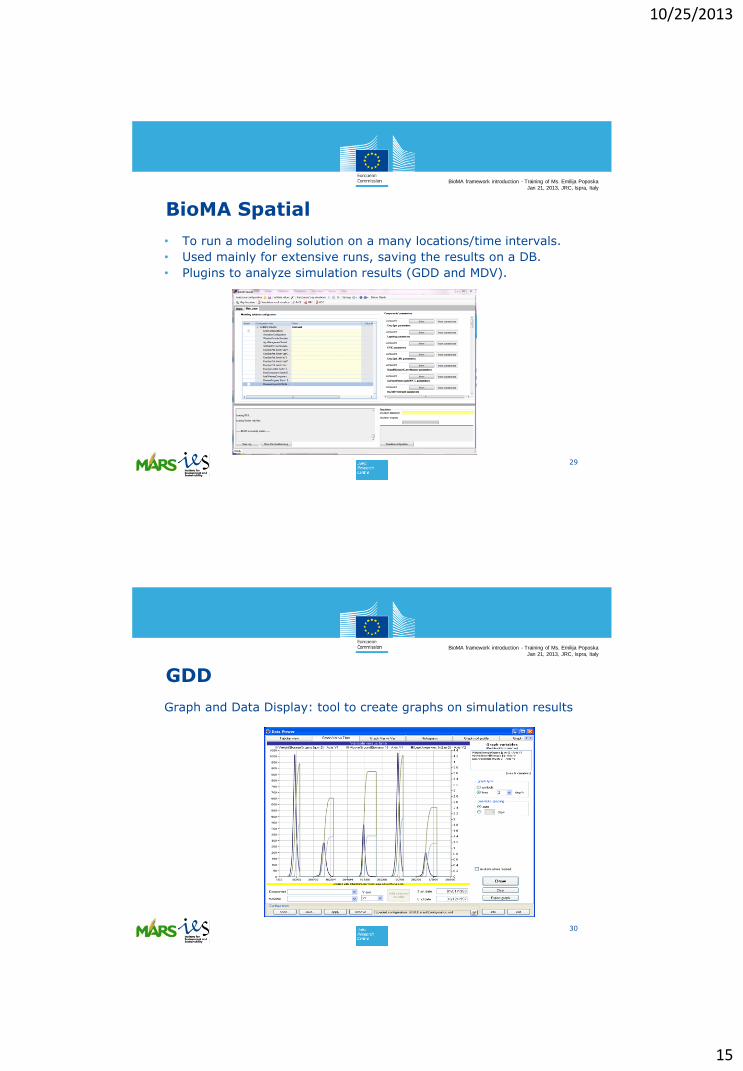
BioMA Spatial
• To run a modeling solution on a many locations/time intervals.
• Used mainly for extensive runs, saving the results on a DB.
• Plugins to analyze simulation results (GDD and MDV).
29
BioMA framework introduction - Training of Ms. Emilija Poposka
Jan 21, 2013, JRC, Ispra, Italy
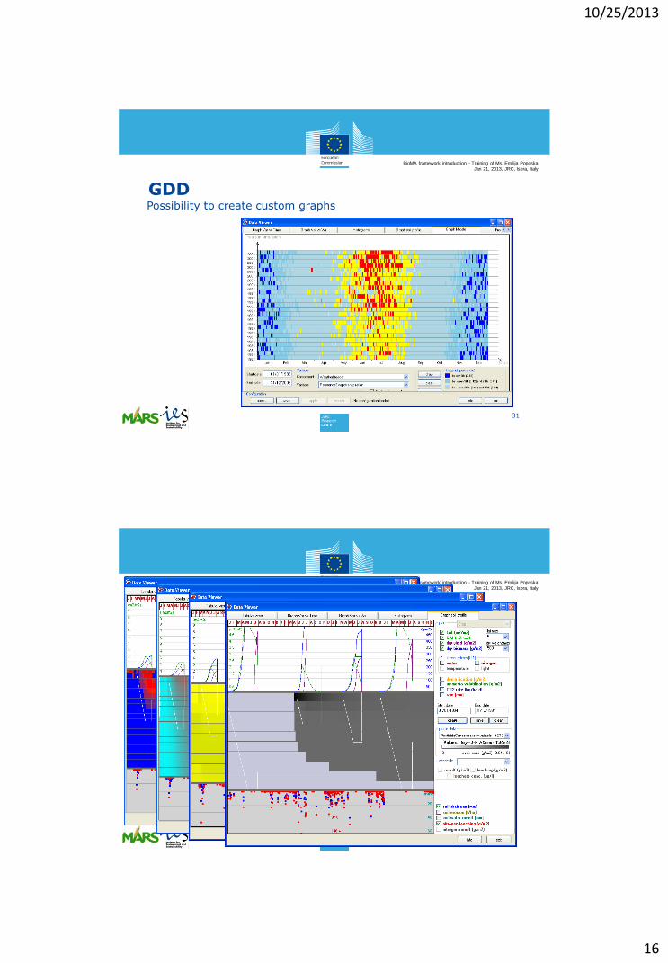
GDD
Graph and Data Display: tool to create graphs on simulation results
30
10/25/2013
16
BioMA framework introduction - Training of Ms. Emilija Poposka
Jan 21, 2013, JRC, Ispra, Italy
31
Possibility to create custom graphs
GDD
BioMA framework introduction - Training of Ms. Emilija Poposka
Jan 21, 2013, JRC, Ispra, Italy
10/25/2013
17
BioMA framework introduction - Training of Ms. Emilija Poposka
Jan 21, 2013, JRC, Ispra, Italy
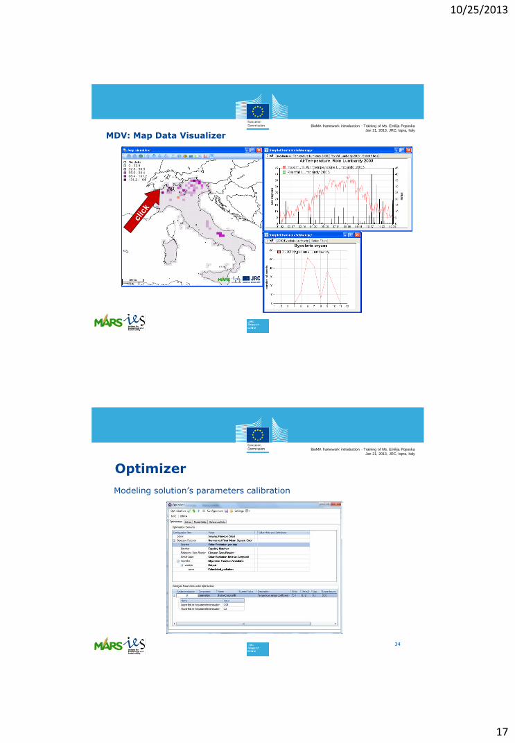
MDV: Map Data Visualizer
BioMA framework introduction - Training of Ms. Emilija Poposka
Jan 21, 2013, JRC, Ispra, Italy
Optimizer
Modeling solution’s parameters calibration
34
10/25/2013
18
BioMA framework introduction - Training of Ms. Emilija Poposka
Jan 21, 2013, JRC, Ispra, Italy
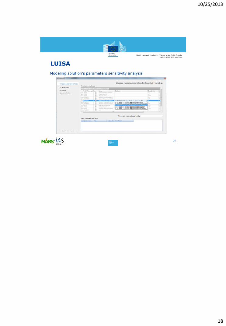
LUISA
Modeling solution’s parameters sensitivity analysis
35

10/25/2013
1
BioMA framework introduction – BASAL Kick off meeting
Mar 26, 2013, JRC, Ispra, Italy
The BioMA framework
Davide Fumagalli
On behalf of the Development Team
Institute for Environment and Sustainability
Joint Research Centre
1
BioMA framework introduction – BASAL Kick off meeting
Mar 26, 2013, JRC, Ispra, Italy
Agronomical model
CROP GROWTH MODEL
Yield
IncomingSolar Radiation
Mean DailyTemperature
Precipitations Management practices
Soil type
Crop variety parameters
Biomass
Crop calendar
LAI/GAI

10/25/2013
2
BioMA framework introduction – BASAL Kick off meeting
Mar 26, 2013, JRC, Ispra, Italy
Modular model (1)
• Model made by different
components
• Each component represents a part
of the physical model
• Some components can be optional
• Components can contain different
approaches to calculate the same
outputs, according to the available
inputs
3
BioMA framework introduction – BASAL Kick off meeting
Mar 26, 2013, JRC, Ispra, Italy
Modular model (2)
• Components must be reusable at
any spatial/time scale
• Independent components are linked
together to create a modeling
solution
4
10/25/2013
3
BioMA framework introduction – BASAL Kick off meeting
Mar 26, 2013, JRC, Ispra, Italy
Composition example
3 components:
• Weather data provider
• CropSyst model
• Frost damage model
=> One modeling solution
Weather data
provider
CropSyst model
Frost damage model
BioMA framework introduction – BASAL Kick off meeting
Mar 26, 2013, JRC, Ispra, Italy
The BioMA platform components:
6
To be
changed
10/25/2013
4
BioMA framework introduction – BASAL Kick off meeting
Mar 26, 2013, JRC, Ispra, Italy
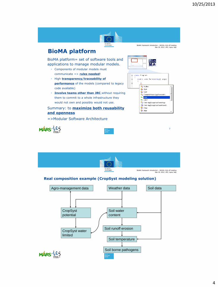
BioMA platform
BioMA platform= set of software tools and
applications to manage modular models.
• Components of modular models must
communicate => rules needed!
• High transparency/traceability of
performance of the models (compared to legacy
code available)
• Involve teams other than JRC without requiring
them to commit to a whole infrastructure they
would not own and possibly would not use.
Summary: to maximize both reusability
and openness
=>Modular Software Architecture
7
BioMA framework introduction – BASAL Kick off meeting
Mar 26, 2013, JRC, Ispra, Italy
Soil borne pathogens
Weather data
CropSyst
potential
Soil water
content
Soil temperature
Soil dataAgro-management data
CropSyst water
limited
Soil runoff erosion
Real composition example (CropSyst modeling solution)
10/25/2013
5
BioMA framework introduction – BASAL Kick off meeting
Mar 26, 2013, JRC, Ispra, Italy
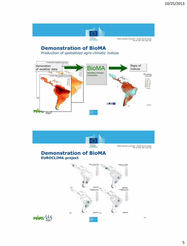
Demonstration of BioMAProduction of spatialized agro-climatic indices
BioMAModelling Solution:
ClimIndices
Generation of weather data
Maps of Indices
BioMA framework introduction – BASAL Kick off meeting
Mar 26, 2013, JRC, Ispra, Italy
Demonstration of BioMAEUROCLIMA project
10
10/25/2013
6
BioMA framework introduction – BASAL Kick off meeting
Mar 26, 2013, JRC, Ispra, Italy
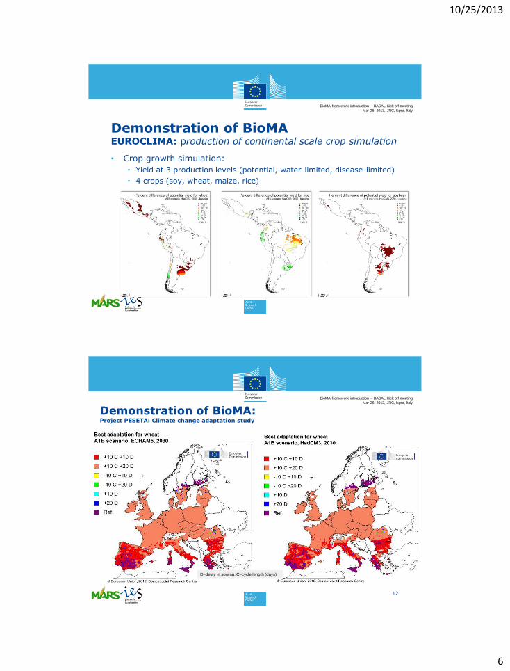
Demonstration of BioMAEUROCLIMA: production of continental scale crop simulation
• Crop growth simulation:
• Yield at 3 production levels (potential, water-limited, disease-limited)
• 4 crops (soy, wheat, maize, rice)
BioMA framework introduction – BASAL Kick off meeting
Mar 26, 2013, JRC, Ispra, Italy
Demonstration of BioMA:Project PESETA: Climate change adaptation study
12
D=delay in sowing, C=cycle length (days)

10/25/2013
7
BioMA framework introduction – BASAL Kick off meeting
Mar 26, 2013, JRC, Ispra, Italy
Data required (1)
Agro-management
data:
• Crop masks
• Sowing date
• Harvest date
• Irrigations
• Other…
13
BioMA framework introduction – BASAL Kick off meeting
Mar 26, 2013, JRC, Ispra, Italy
Data required (2)
Crop data:
• Crop varieties
distribution
• Variety
parameters
14
Rapeseed varieties in CGMS
10/25/2013
8
BioMA framework introduction – BASAL Kick off meeting
Mar 26, 2013, JRC, Ispra, Italy
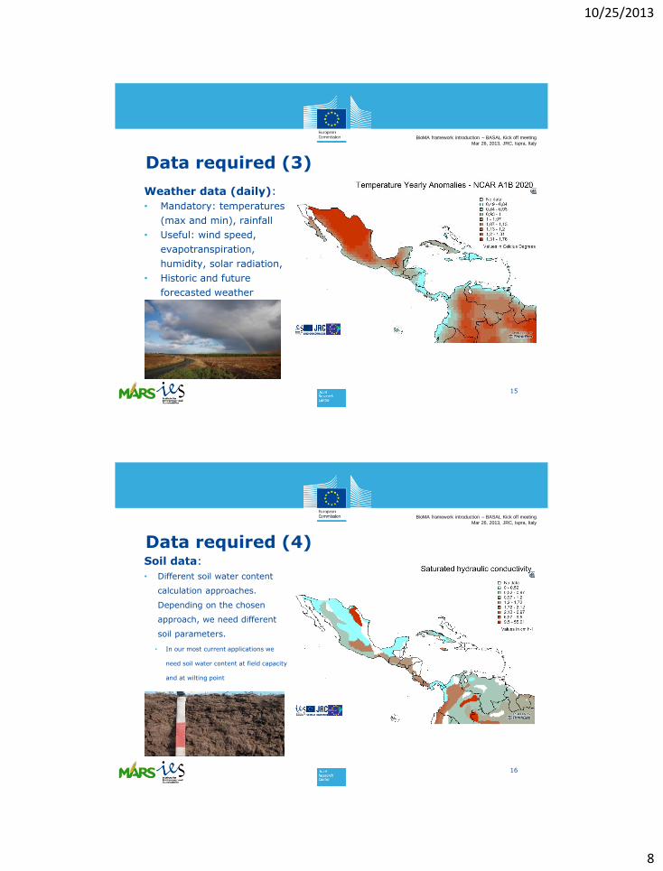
Data required (3)
Weather data (daily):
• Mandatory: temperatures
(max and min), rainfall
• Useful: wind speed,
evapotranspiration,
humidity, solar radiation,
• Historic and future
forecasted weather
15
BioMA framework introduction – BASAL Kick off meeting
Mar 26, 2013, JRC, Ispra, Italy
Data required (4)Soil data:
• Different soil water content
calculation approaches.
Depending on the chosen
approach, we need different
soil parameters.
• In our most current applications we
need soil water content at field capacity
and at wilting point
16
10/25/2013
9
BioMA framework introduction – BASAL Kick off meeting
Mar 26, 2013, JRC, Ispra, Italy
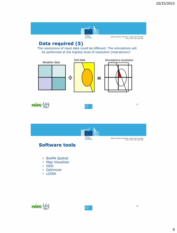
Data required (5)The resolutions of input data could be different. The simulations will
be performed at the highest level of resolution (intersection)
17
Weather dataSoil data Simulations resolution
BioMA framework introduction – BASAL Kick off meeting
Mar 26, 2013, JRC, Ispra, Italy
Software tools
18
• BioMA Spatial• Map Visualizer• GDD• Optimizer• LUISA
10/25/2013
10
BioMA framework introduction – BASAL Kick off meeting
Mar 26, 2013, JRC, Ispra, Italy
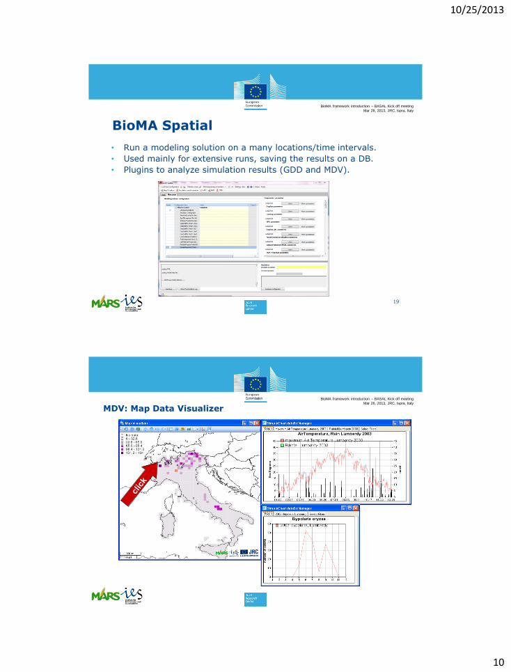
BioMA Spatial
• Run a modeling solution on a many locations/time intervals.
• Used mainly for extensive runs, saving the results on a DB.
• Plugins to analyze simulation results (GDD and MDV).
19
BioMA framework introduction – BASAL Kick off meeting
Mar 26, 2013, JRC, Ispra, Italy
MDV: Map Data Visualizer
10/25/2013
11
BioMA framework introduction – BASAL Kick off meeting
Mar 26, 2013, JRC, Ispra, Italy
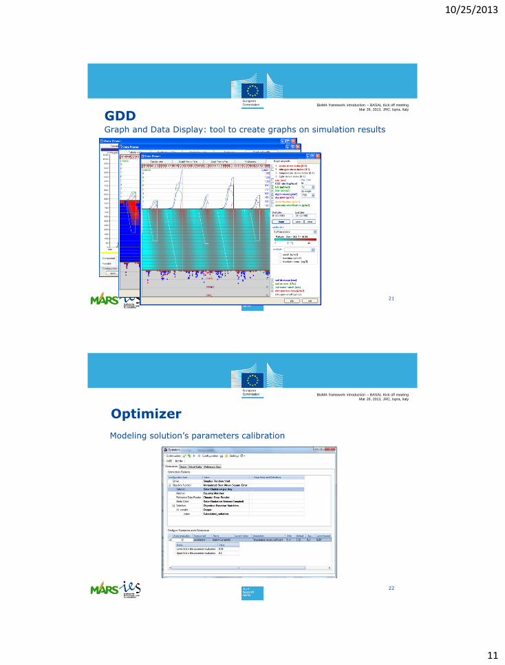
GDDGraph and Data Display: tool to create graphs on simulation results
21
BioMA framework introduction – BASAL Kick off meeting
Mar 26, 2013, JRC, Ispra, Italy
Optimizer
Modeling solution’s parameters calibration
22
10/25/2013
12
BioMA framework introduction – BASAL Kick off meeting
Mar 26, 2013, JRC, Ispra, Italy
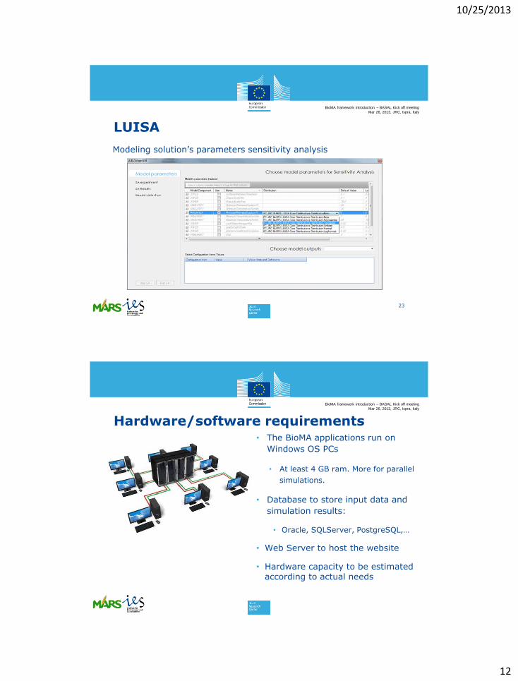
LUISA
Modeling solution’s parameters sensitivity analysis
23
BioMA framework introduction – BASAL Kick off meeting
Mar 26, 2013, JRC, Ispra, Italy
Hardware/software requirements• The BioMA applications run on
Windows OS PCs
• At least 4 GB ram. More for parallel
simulations.
• Database to store input data and
simulation results:
• Oracle, SQLServer, PostgreSQL,…
• Web Server to host the website
• Hardware capacity to be estimated according to actual needs

10/25/2013
13
BioMA framework introduction – BASAL Kick off meeting
Mar 26, 2013, JRC, Ispra, Italy
Human resources• Analysts/agronomists to run the
model and evaluate simulation
results
• IT professional to modify the code
of models and tools according to
specific needs
• IT system administrator to
manage the servers

1
BioMA – Biophysical Models Application
Overview
Fabien Ramos
On behalf of the development Team
25 October 2013 1
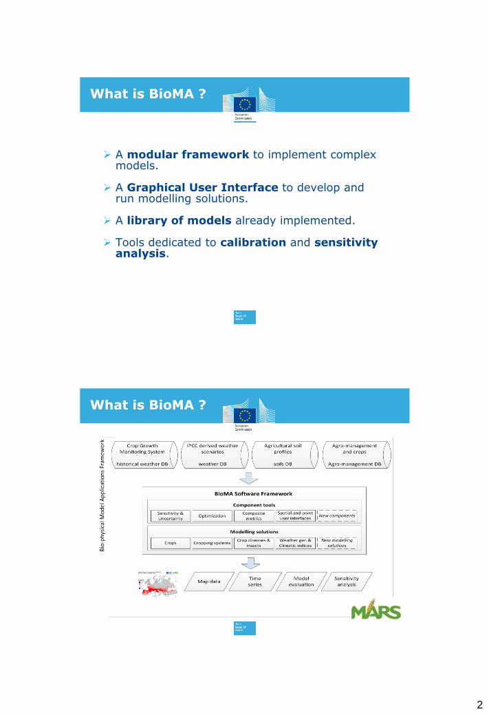
BioMA is a platform that aims to give support in
parameterizing, running and analyzing crop
model simulations.
What is BioMA ?
2
A modular framework to implement complexmodels.
A Graphical User Interface to develop and run modelling solutions.
A library of models already implemented.
Tools dedicated to calibration and sensitivityanalysis.
What is BioMA ?
What is BioMA ?
3
A Modular Architecture
A modular conceptualization of models allows:
An easier transfer of research results to operational tools;
The comparison of different approaches;
More rapid application development;
Re-use of models of known quality;
Independent extensibility by third parties;
Avoiding duplication.
A modulararchitecture
4
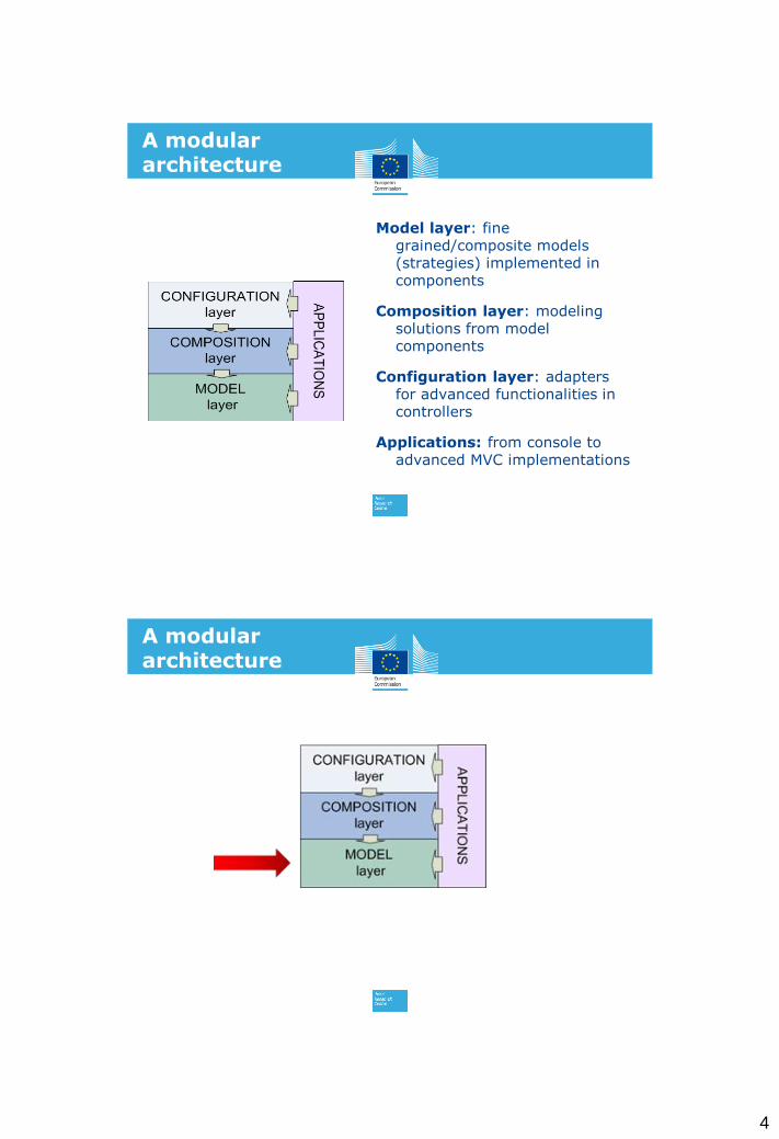
A modulararchitecture
Model layer: fine grained/composite models (strategies) implemented in components
Composition layer: modeling solutions from model components
Configuration layer: adapters for advanced functionalities in controllers
Applications: from console to advanced MVC implementations
A modulararchitecture
5
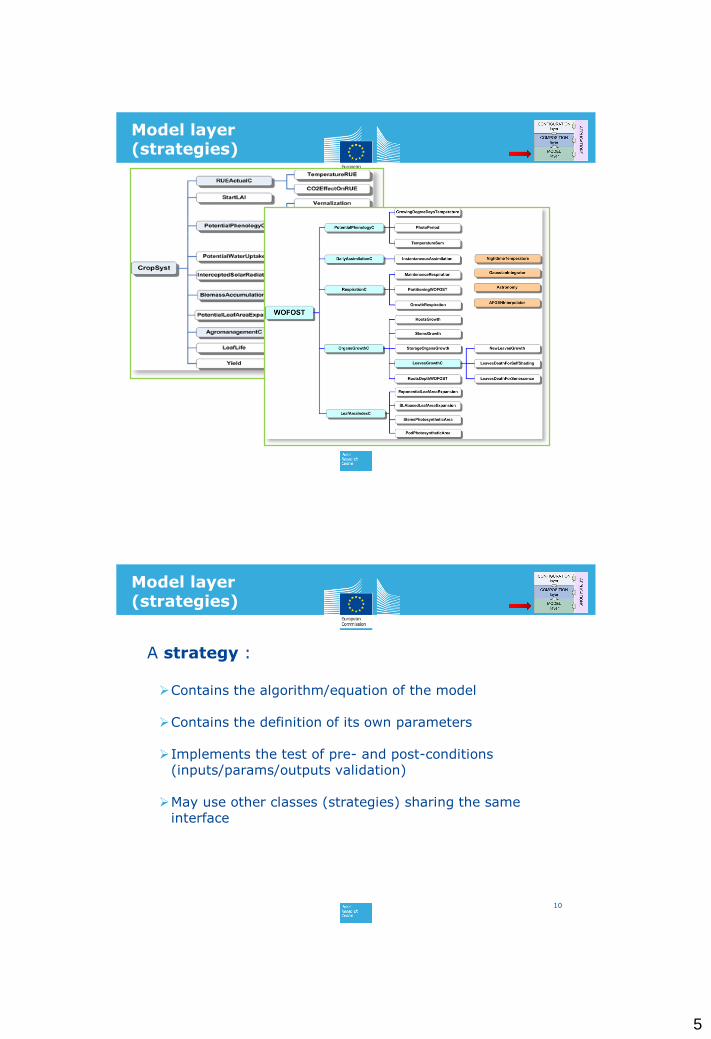
Model layer (strategies)
A strategy :
Contains the algorithm/equation of the model
Contains the definition of its own parameters
Implements the test of pre- and post-conditions (inputs/params/outputs validation)
May use other classes (strategies) sharing the same interface
10
Model layer (strategies)

6
A modulararchitecture
Composition layer (Modelling Solutions)
A composition layer allows linking model components to build modelling solutions;
A modelling solution is developed and used for a specific purpose (e.g. a “crop model” in which we link crop, soil water and other components to simulate water
limited production of crops);
The composition layer include Time and Event handling.

7
Water
Erosion
Temperature
SOIL
Weather
Agro-management Diseases
Composition layer (Modelling Solutions)
Modelling Solutions
Water
Erosion
Temperature
SOIL
Weather
Agro-management
Modellingsolution
Diseases

8
A modulararchitecture
The Configuration layer :
Allows setting configuration values at run time;
Allows validating configurations;
Serializes/deserializes configurations;
Allows running modeling solutions;
Triggers events when the configuration is changed, to be used by a
controller in a MVC application;
Does not have any dependency from the composition layer;
Allows iteration (space, time, optimization…);
Requires simple implementation to build adapters.
Configuration layer

9
Water
Erosion
Temperature
SOIL
Weather
Agro-managementModellingsolution
Diseases
Configuration layer
XML
WeatherDB
SoilDB
The strategies are the building blocs of the models, they belong to the
model layer. They can be simple or composite when they call other
strategies.
A component is a library of strategies dedicated to model a specific
process. For instance the strategies used for the modelling of soil erosion
and runoff are included in the component SoilRE.
A modelling solution is obtained when the components are connected and
possibly configured to run a simulation. The terminology « modelling
solution » is used indifferently at composition layer and configuration
layer.
Models can refer to strategies or modelling solutions.
Terminology

10
Graphical User Interface
GUI
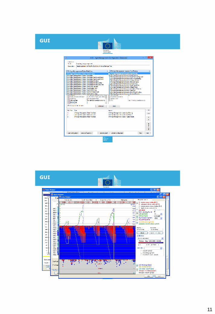
11
GUI
GUI

12
Models ready for BioMA
What is BioMA ?
Crop models available
CropSyst (Generic crop/cropping systems simulator)
WOFOST (Generic crop simulator)
WARM (Rice simulation)
STICS (Generic crop / Grassland simulator)
CANEGRO (Sugarcane)
Plant growthmodels

13
and some other components…
PotentialDiseaseInfection (Airborne plant diseases)
PotentialSoilDiseaseInfection (Soilborne plant diseases)
MYMICS (Mycotoxin maize)
GrainQuality (Currently rice)
ClimIndices (Climatic indices)
Run a simulation
ClimIndices is a component containing routines to calculate
weather indicators from multi-year series of daily
weather data.
Basic indicators are computed as simple statistics on weather
inputs (yearly series of daily precipitation, maximum and
minimum air temperatures, incoming solar radiation, and
reference evapotranspiration).
Other indicators are derived, grouped into six classes: dates,
counts, thermal sums, water, waves, indices.
Climate indices

14
The libraries currently available
27
Weather libraries
• AirTemperature, EvapoTranspiration, LeafWetness• Climate indices• Weather Generation (ClimGen, CLIMAK) • …
Plant libraries
• Generic crop Simulation (CropSyst, WOFOST)• Pasture (STIC)• Rice (WARM)• SugarCane (CANEGRO)• …
Soil libraries
• Soil water runoff and erosion• Soil water redistribution (cascading,
FiniteDifferences)• Soil surface and profile temperature• Soil Nitrogen• Pedotransfer functions• …
Agriculture management
• Rule based modelling
StressesAbiotic• Heat damage• Frost kill• Rice cold shocks• Lodging• …
Biotic• Generic air-borne diseases• Generic soil-borne diseases• CornBorer simulator• …
Tools
What is BioMA ?

15
IMMA: A tool for comparing simulation results to reference data
(e.g. time series)
Optimizer: A tool for calibration and parameter optimization
LUISA : A tool for sensitivity analysis (Morits, Sobol …)
Tools
Documentation
What is BioMA ?

16
Framework documentation
Weather
Air Temperature Rain
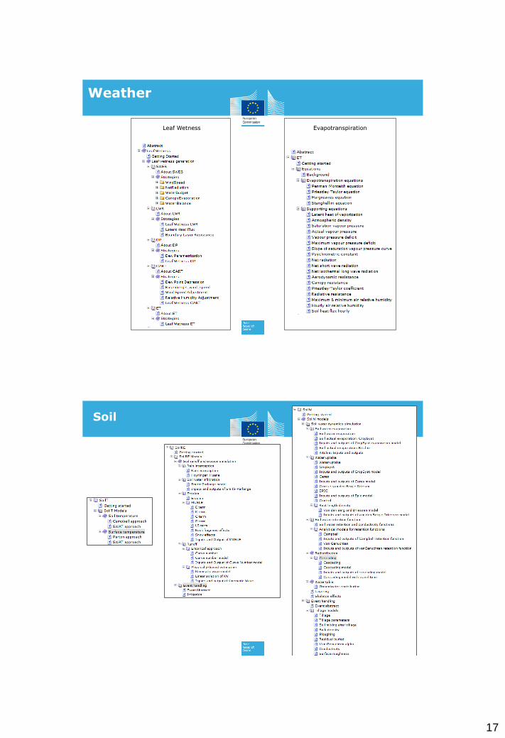
17
Leaf Wetness Evapotranspiration
Weather
Soil
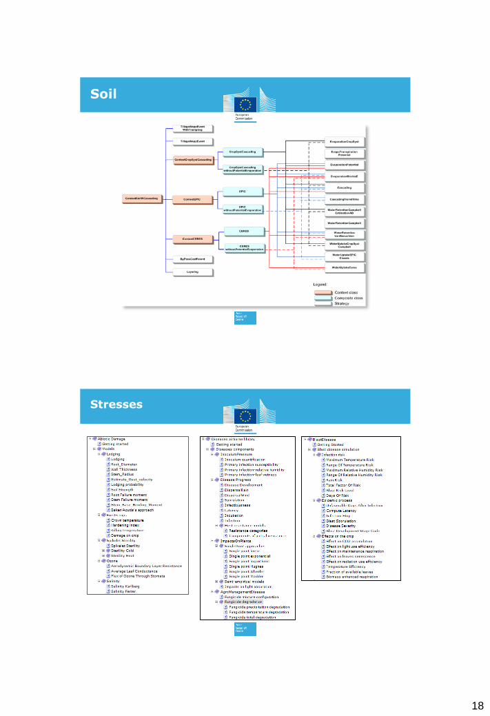
18
Models ready for BioMA
Soil
Stresses

19
To run an existing modelling solution and look at the results;
To implement some strategies (Model layer);
To build a new modelling solution (Composition layer);
To configure a modelling solution and run it (Configuration layer).
Tasks of the week
Thank you
3825 October 2013
Contact :
Documentation:
http://bioma.jrc.ec.europa.eu/bioma/help/
http://agsys.cra-cin.it/tools/default.aspx
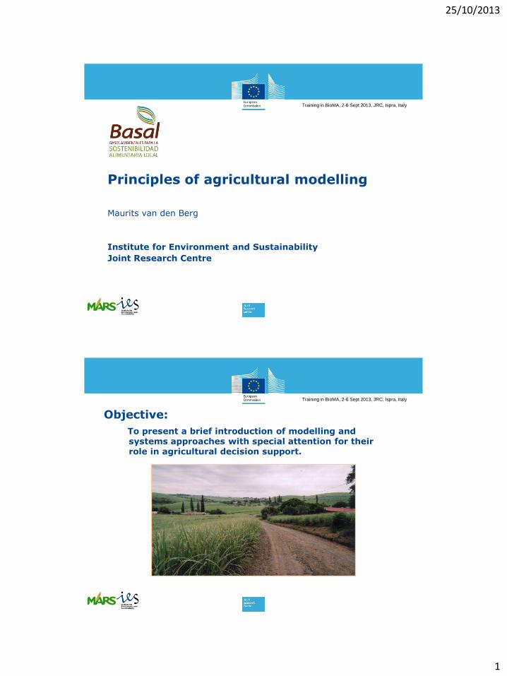
25/10/2013
1
Training in BioMA, 2-6 Sept 2013, JRC, Ispra, Italy
Principles of agricultural modelling
Maurits van den Berg
Institute for Environment and Sustainability
Joint Research Centre
Training in BioMA, 2-6 Sept 2013, JRC, Ispra, Italy
Objective:
To present a brief introduction of modelling and systems approaches with special attention for their role in agricultural decision support.

25/10/2013
2
Training in BioMA, 2-6 Sept 2013, JRC, Ispra, Italy
Contents
• Types of models (for decision support)
• Dynamic, numerical, computer-based, mechanistic, simulation models
• Crop growth models
• The role of models in agricultural decision making
• The use of models in agricultural decision making
Training in BioMA, 2-6 Sept 2013, JRC, Ispra, Italy
Objective:
To present a brief introduction of modelling and systems approaches with special attention for their role in agricultural decision support.
25/10/2013
3
Training in BioMA, 2-6 Sept 2013, JRC, Ispra, Italy
Mental models
? = f ( ? , ? , ? )
Types of models (for decision support)
Training in BioMA, 2-6 Sept 2013, JRC, Ispra, Italy
Flow Chart for Decision Support
DOES THE
DEVICE WORK
YES NO
NO
NO
NO
NO
YES
YES
YES
NO
PROBLEM
DON’T MESS
WITH IT
DID YOU
MESS
WITH IT
WILL YOU
GET
FIRED?
TRASH IT
CAN YOU BLAME
SOMEONE ELSE?
HIDE ITDOES ANYONE
KNOW?
YOU
POOR
IDIOT
YOU
IDIOT
YES

25/10/2013
4
Training in BioMA, 2-6 Sept 2013, JRC, Ispra, Italy
(Computer based) mathematical models
Static - e.g. models for fertiliser recommendation based on soil/plant analysis
Dynamic - e.g. crop growth (simulation) models
Training in BioMA, 2-6 Sept 2013, JRC, Ispra, Italy
Strengths and Weaknesses
Type Versatility Speed Ease of
use
Objective /
reproducible Quantified Human
aspects Dynamic
Mental models ++ ++ / -- ++ - - ++ +
Decision trees - 0 + ++ - - -
Computer-based
dynamic + + / ++ - ++ ++ - ++

25/10/2013
5
Training in BioMA, 2-6 Sept 2013, JRC, Ispra, Italy
Conclusions
• All our decisions are supported by models
• Computer-based models are just one specific type (or family) of models
• We must have good reasons to use them
Training in BioMA, 2-6 Sept 2013, JRC, Ispra, Italy
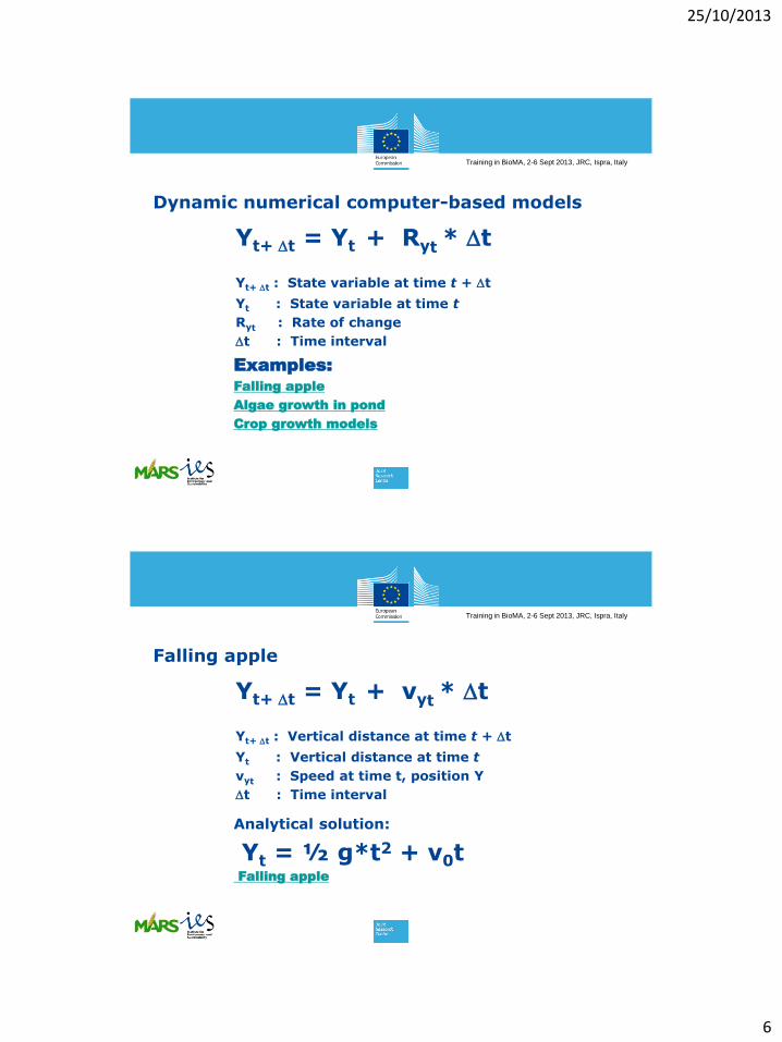
Yt+ t = Yt + Ryt * t
Yt+ t : State variable at time t + t
Yt : State variable at time t
Ryt : Rate of change
t : Time interval
Dynamic numerical computer-based models
25/10/2013
6
Training in BioMA, 2-6 Sept 2013, JRC, Ispra, Italy
Examples:
Falling apple
Algae growth in pond
Crop growth models
Yt+ t = Yt + Ryt * t
Yt+ t : State variable at time t + t
Yt : State variable at time t
Ryt : Rate of change
t : Time interval
Dynamic numerical computer-based models
Training in BioMA, 2-6 Sept 2013, JRC, Ispra, Italy
Analytical solution:
Yt = ½ g*t2 + v0tFalling apple
Yt+ t = Yt + vyt * t
Yt+ t : Vertical distance at time t + t
Yt : Vertical distance at time t
vyt : Speed at time t, position Y
t : Time interval
Falling apple

25/10/2013
7
Training in BioMA, 2-6 Sept 2013, JRC, Ispra, Italy
Algae growth in pond
Yt+ t = Yt + (gyt - dyt ) * t
Yt+ t : Algae biomass at time t + t (g.l-1)
Yt : Algae biomass at time t
gyt : rate of new biomass growth (g.l-1.d-1)
dyt : death rate (g.l-1.d-1)
t : Time interval (d)
Algae growth in pond
Training in BioMA, 2-6 Sept 2013, JRC, Ispra, Italy
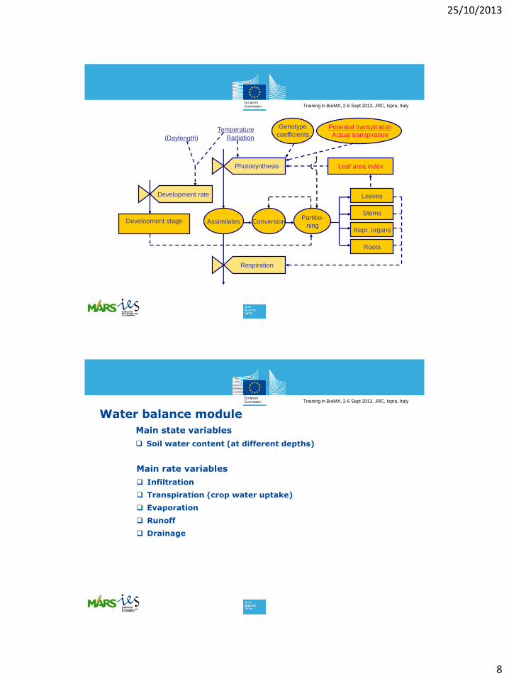
Crop growth models
Main state variables
Development stage
Leaf area index (LAI)
Leaf biomass
Stem biomass
Storage organs (e.g. grain) biomass
Root biomass
Main rate variables
Development rate
Photosynthesis
Respiration (growth, maintenance)
Rate of LAI change
Change in biomass of leaves, stems, storage organs, roots
25/10/2013
8
Training in BioMA, 2-6 Sept 2013, JRC, Ispra, Italy
Photosynthesis
Respiration
Leaf area index
Genotype
coefficientsTemperature
Radiation
Assimilates ConversionPartitio-
ning
Leaves
Stems
Repr. organs
Roots
Development rate
Development stage
(Daylength)
Potential transpiration
Actual transpiration
Training in BioMA, 2-6 Sept 2013, JRC, Ispra, Italy
Water balance module
Main state variables
Soil water content (at different depths)
Main rate variables
Infiltration
Transpiration (crop water uptake)
Evaporation
Runoff
Drainage
25/10/2013
9
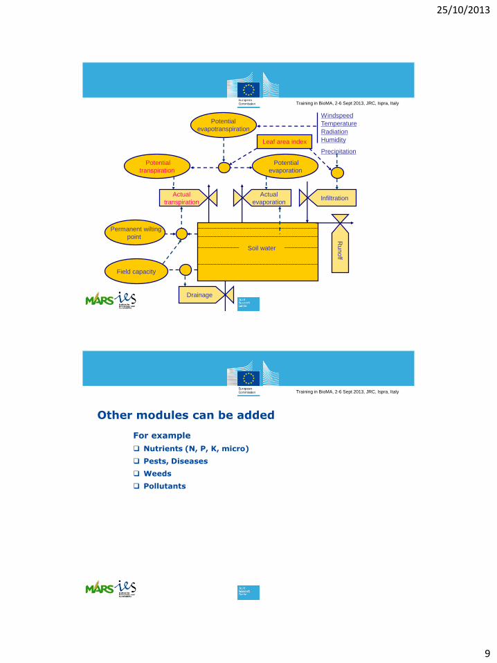
Training in BioMA, 2-6 Sept 2013, JRC, Ispra, Italy
Windspeed
Temperature
Radiation
Humidity
Potential
evapotranspiration
Actual
transpiration
Actual
evaporation
Drainage
Soil water
Potential
evaporation
Infiltration
Runoff
Field capacity
Permanent wilting
point
Potential
transpiration
Leaf area index
Precipitation
Training in BioMA, 2-6 Sept 2013, JRC, Ispra, Italy
Other modules can be added
For example
Nutrients (N, P, K, micro)
Pests, Diseases
Weeds
Pollutants
25/10/2013
10
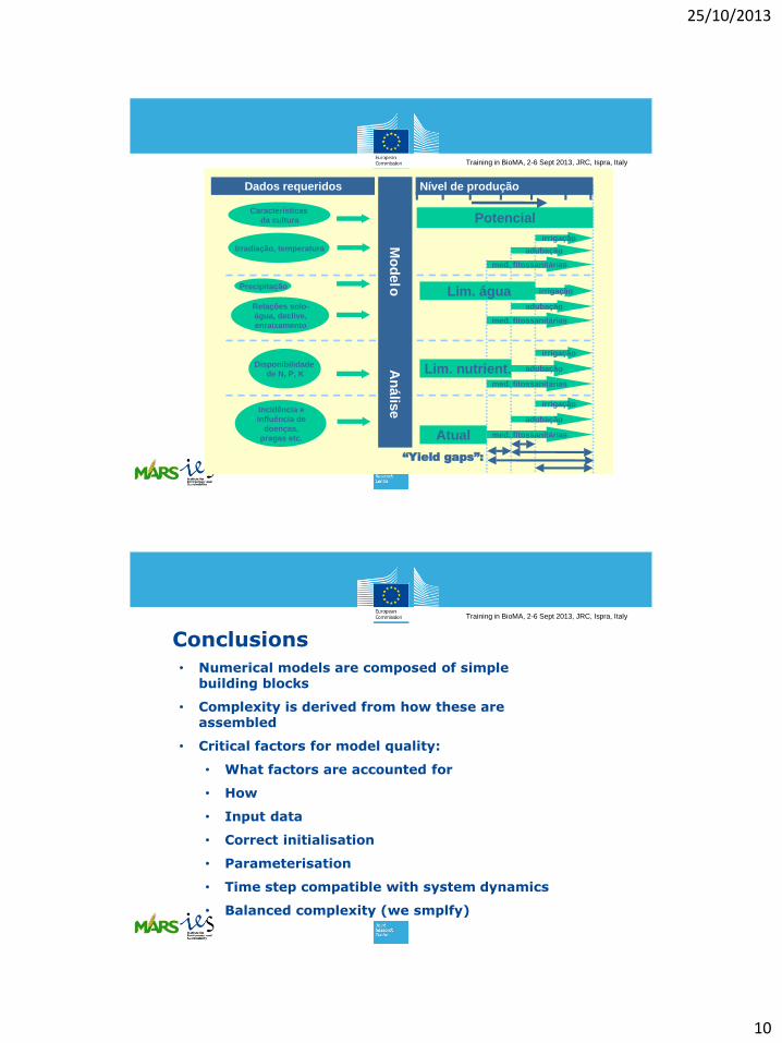
Training in BioMA, 2-6 Sept 2013, JRC, Ispra, Italy
Características
da cultura
Irradiação, temperatura
Water limited
med. fitossanitárias
adubação
irrigação
Disponibilidade
de N, P, K Lim. nutrient.
Precipitação
Relações solo-
água, declive,
enraizamento
Lim. água
Potencial
med. fitossanitárias
adubação
irrigação
med. fitossanitárias
adubação
irrigação
Incidência e
influência de
doenças,
pragas etc. med. fitossanitárias
adubação
irrigação
Atual
Dados requeridos Nível de produção
Mo
de
loA
ná
lise
“Yield gaps”:
Training in BioMA, 2-6 Sept 2013, JRC, Ispra, Italy
Conclusions
• Numerical models are composed of simple building blocks
• Complexity is derived from how these are assembled
• Critical factors for model quality:
• What factors are accounted for
• How
• Input data
• Correct initialisation
• Parameterisation
• Time step compatible with system dynamics
• Balanced complexity (we smplfy)

25/10/2013
11
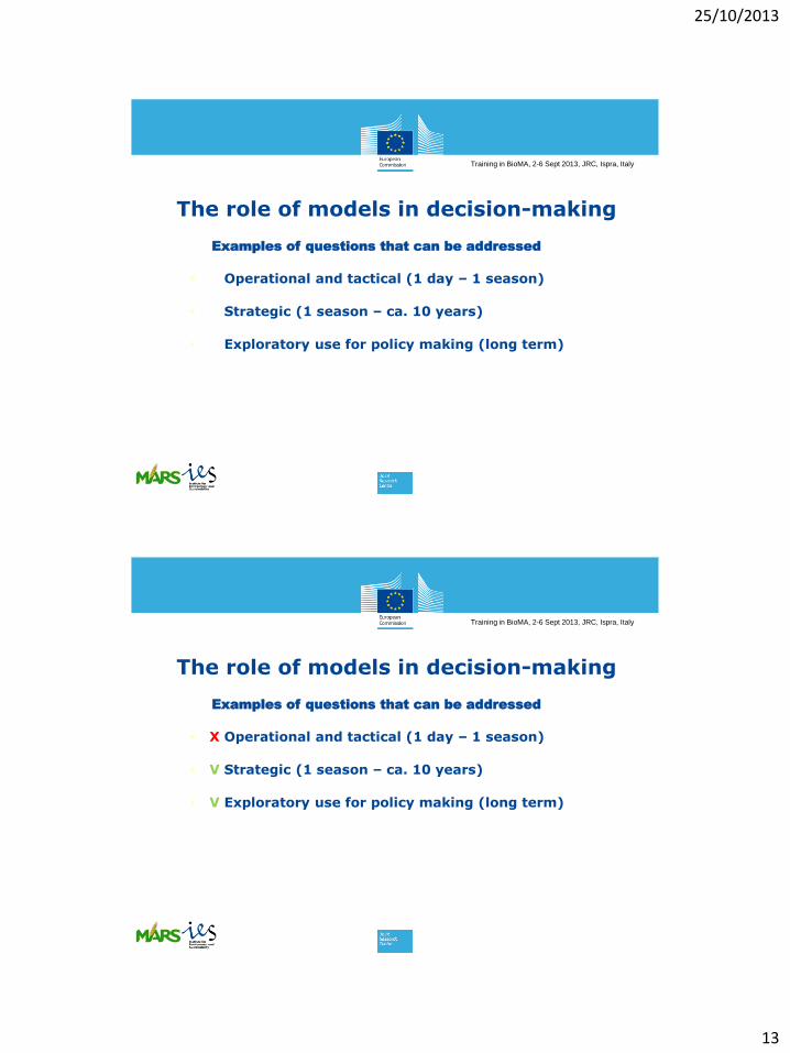
Training in BioMA, 2-6 Sept 2013, JRC, Ispra, Italy
Operational and tactical (1 day – 1 season)
Strategic (1 season – ca. 10 years)
Exploratory use for policy making (long term)
Examples of questions that can be addressed
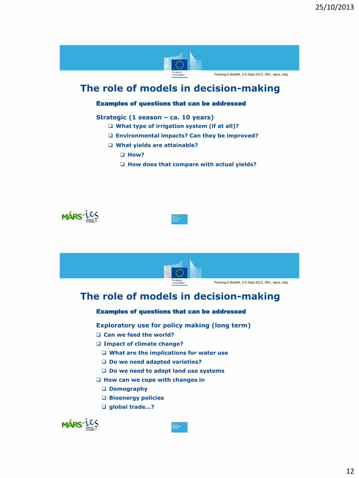
The role of models in decision-making
Training in BioMA, 2-6 Sept 2013, JRC, Ispra, Italy
Operational and tactical (1 day – 1 season)
The best time of planting and harvesting?
Beginning and end of milling season?
How much grain can we sell at contract?
Irrigation: how? when? how much?
How much nitrogen and when?
Risk of pests?
Yields expected world-wide? Impact on prices?
Examples of questions that can be addressed
The role of models in decision-making
25/10/2013
12
Training in BioMA, 2-6 Sept 2013, JRC, Ispra, Italy
Strategic (1 season – ca. 10 years)
What type of irrigation system (if at all)?
Environmental impacts? Can they be improved?
What yields are attainable?
How?
How does that compare with actual yields?
Examples of questions that can be addressed
The role of models in decision-making
Training in BioMA, 2-6 Sept 2013, JRC, Ispra, Italy
Exploratory use for policy making (long term)
Can we feed the world?
Impact of climate change?
What are the implications for water use
Do we need adapted varieties?
Do we need to adapt land use systems
How can we cope with changes in
Demography
Bioenergy policies
global trade…?
Examples of questions that can be addressed
The role of models in decision-making
25/10/2013
13
Training in BioMA, 2-6 Sept 2013, JRC, Ispra, Italy
X Operational and tactical (1 day – 1 season)
V Strategic (1 season – ca. 10 years)
V Exploratory use for policy making (long term)
Examples of questions that can be addressed
The role of models in decision-making
Training in BioMA, 2-6 Sept 2013, JRC, Ispra, Italy
X Operational and tactical (1 day – 1 season)
V Strategic (1 season – ca. 10 years)
V Exploratory use for policy making (long term)
Examples of questions that can be addressed
The role of models in decision-making
25/10/2013
14
Training in BioMA, 2-6 Sept 2013, JRC, Ispra, Italy
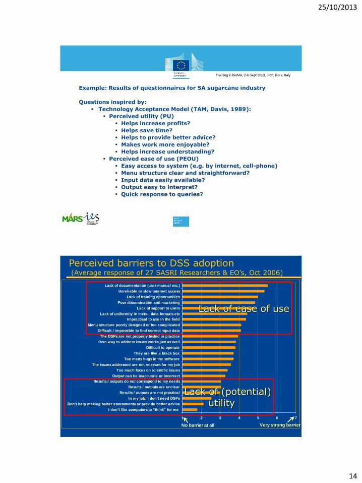
Example: Results of questionnaires for SA sugarcane industry
Questions inspired by:
Technology Acceptance Model (TAM, Davis, 1989):
Perceived utility (PU)
Helps increase profits?
Helps save time?
Helps to provide better advice?
Makes work more enjoyable?
Helps increase understanding?
Perceived ease of use (PEOU)
Easy access to system (e.g. by internet, cell-phone)
Menu structure clear and straightforward?
Input data easily available?
Output easy to interpret?
Quick response to queries?
Training in BioMA, 2-6 Sept 2013, JRC, Ispra, Italy
1 2 3 4 5 6 7
I don’t like computers to “think” for me
Don’t help making better assessments or provide better advice
In my job, I don’t need DSPs
Results / outputs are not practical
Results / outputs are unclear
Results / outputs do not correspond to my needs
Output can be inaccurate or incorrect
Too much focus on scientific issues
The issues addressed are not relevant for my job
Too many bugs in the software
They are like a black box
Difficult to operate
Own way to address issues works just as well
The DSPs are not properly tested in practice
Difficult / impossible to find correct input data
Menu structure poorly designed or too complicated
Impractical to use in the field
Lack of uniformity in menu, data formats etc
Lack of support to users
Poor dissemination and marketing
Lack of training opportunities
Unreliable or slow internet access
Lack of documentation (user manual etc.)
Very strong barrierNo barrier at all
Perceived barriers to DSS adoption(Average response of 27 SASRI Researchers & EO’s, Oct 2006)
Lack of ease of use
Lack of (potential)utility
25/10/2013
15
Training in BioMA, 2-6 Sept 2013, JRC, Ispra, Italy
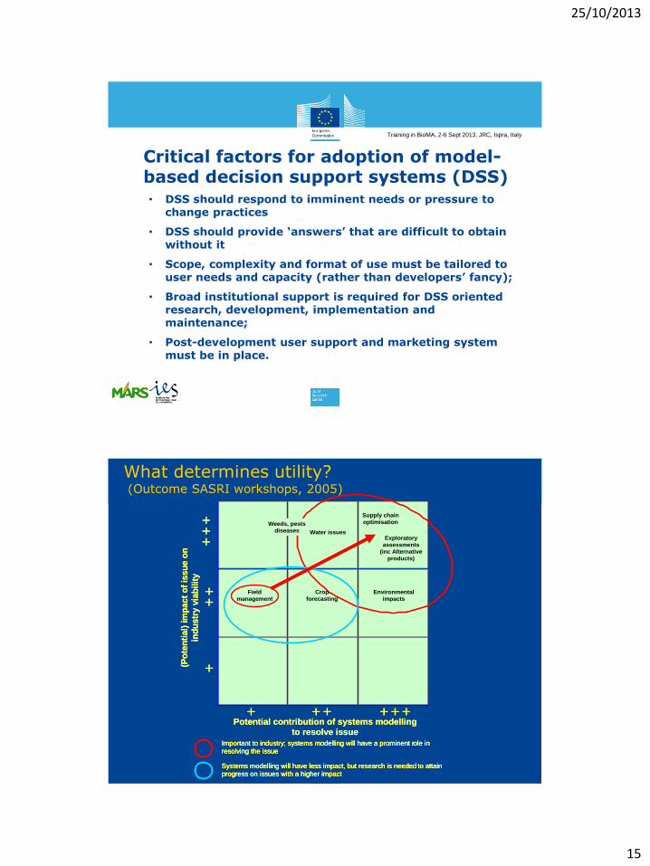
Critical factors for adoption of model-based decision support systems (DSS)• DSS should respond to imminent needs or pressure to
change practices
• DSS should provide ‘answers’ that are difficult to obtain without it
• Scope, complexity and format of use must be tailored to user needs and capacity (rather than developers’ fancy);
• Broad institutional support is required for DSS oriented research, development, implementation and maintenance;
• Post-development user support and marketing system must be in place.
Training in BioMA, 2-6 Sept 2013, JRC, Ispra, Italy
Potential contribution of systems modelling
to resolve issue
(Po
ten
tial)
im
pact
of
issu
e o
n
ind
ustr
y v
iab
ilit
y
++
++
+
+ ++ +++
+
Supply chain
optimisation
Exploratory
assessments
(inc Alternative
products)
Environmental
impacts
Field
management
Weeds, pests
diseases
Important to industry; systems modelling will have a prominent role in
resolving the issue
Systems modelling will have less impact, but research is needed to attain
progress on issues with a higher impact
Water issues
Crop
forecasting
Potential contribution of systems modelling
to resolve issue
(Po
ten
tial)
im
pact
of
issu
e o
n
ind
ustr
y v
iab
ilit
y
++
++
+
+ ++ +++
+
Supply chain
optimisation
Exploratory
assessments
(inc Alternative
products)
Environmental
impacts
Field
management
Weeds, pests
diseases
Important to industry; systems modelling will have a prominent role in
resolving the issue
Systems modelling will have less impact, but research is needed to attain
progress on issues with a higher impact
Important to industry; systems modelling will have a prominent role in
resolving the issue
Systems modelling will have less impact, but research is needed to attain
progress on issues with a higher impact
Water issues
Crop
forecasting
What determines utility?(Outcome SASRI workshops, 2005)

25/10/2013
16
Training in BioMA, 2-6 Sept 2013, JRC, Ispra, Italy
Conclusions
• Computer-based agricultural models have a role to play in operational, technical and strategic decision making as well as in exploratory studies
• So far they are underutilised for operational decision support
• Critical adoption factors need to be taken into account during all stages of development and after release
25/10/2013
1
Training in BioMA, 2-6 Sept 2013, JRC, Ispra, Italy
WOFOST
Maurits van den Berg
Institute for Environment and Sustainability
Joint Research Centre
Training in BioMA, 2-6 Sept 2013, JRC, Ispra, Italy
WOFOST
Development started in early 1980’s as part of WOrld
FOod Studies initiative; released in 1988
Developed by Wageningen University and Research
Centre (current maintenance Alterra)
http://www.wageningenur.nl/en/Expertise-
Services/Research-Institutes/alterra/Facilities-
Products/Software/WOFOST/Documentation-
WOFOST.htm
2

25/10/2013
2
Training in BioMA, 2-6 Sept 2013, JRC, Ispra, Italy
WOFOST
Main characteristics
Generic model, many crops can be (and are) simulated
Point model
Dynamic, numerical integration; one-day time step
Simulates potential growth and water-limited growth
Process descriptions based as much as possible on
universally valid bio-physical laws
Differences between crops expressed in “easily
interpreted” model parameters
Used as starting point for many other models
25 October 2013
Training in BioMA, 2-6 Sept 2013, JRC, Ispra, Italy
Yt+ t = Yt + Ryt * t
Yt+ t : State variable at time t + t
Yt : State variable at time t
Ryt : Rate of change
t : Time interval
Dynamic numerical computer-based models

25/10/2013
3
Training in BioMA, 2-6 Sept 2013, JRC, Ispra, Italy
Main state variables
Development stage
Leaf area index (LAI)
Leaf biomass
Stem biomass
Storage organs (e.g. grain) biomass
Root biomass
Main rate variables
Development rate
Photosynthesis
Respiration (growth, maintenance)
Leaf senescence, root senescence
Change in biomass of leaves, stems, storage organs, roots
Training in BioMA, 2-6 Sept 2013, JRC, Ispra, Italy
Photosynthesis
Respiration
Leaf area index
Genotype
coefficientsTemperature
Radiation
Assimilates ConversionPartitio-
ning
Leaves
Stems
Repr. organs
Roots
Development rate
Development stage
(Daylength)
Potential transpiration
Actual transpiration
25/10/2013
4
Training in BioMA, 2-6 Sept 2013, JRC, Ispra, Italy
7
Training in BioMA, 2-6 Sept 2013, JRC, Ispra, Italy
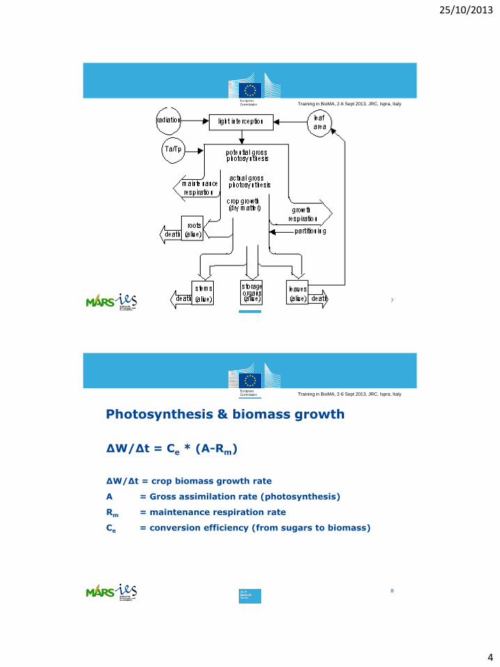
Photosynthesis & biomass growth
8
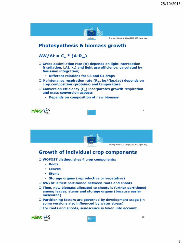
ΔW/Δt = Ce * (A-Rm)
ΔW/Δt = crop biomass growth rate
A = Gross assimilation rate (photosynthesis)
Rm = maintenance respiration rate
Ce = conversion efficiency (from sugars to biomass)
25/10/2013
5
Training in BioMA, 2-6 Sept 2013, JRC, Ispra, Italy
Photosynthesis & biomass growth
9
ΔW/Δt = Ce * (A-Rm)
Gross assimilation rate (A) depends on light interception f(radiation, LAI, ke) and light use efficiency; calculated by Gaussian integration;
• Different relations for C3 and C4 crops
Maintenance respiration rate (Rm, kg/(kg.day) depends on crop composition (proteins) and temperature
Conversion efficiency (Ce) incorporates growth respiration and mass conversion aspects
• Depends on composition of new biomass
Training in BioMA, 2-6 Sept 2013, JRC, Ispra, Italy
Growth of individual crop components
10
WOFOST distinguishes 4 crop components:
• Roots
• Leaves
• Stems
• Storage organs (reproductive or vegetative)
ΔW/Δt is first partitioned between roots and shoots
Then, new biomass allocated to shoots is further partitioned among leaves, stems and storage organs (because easier measured)
Partitioning factors are governed by development stage (in some versions also influenced by water stress)
For roots and shoots, senescence is taken into account.

25/10/2013
6
Training in BioMA, 2-6 Sept 2013, JRC, Ispra, Italy
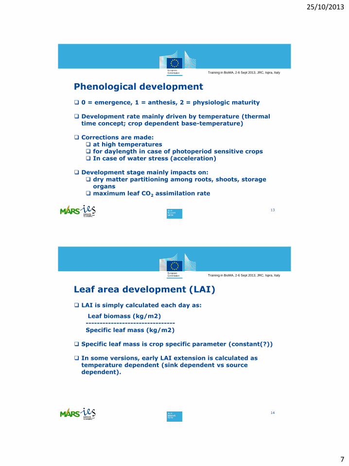
Phenological development
11
0 = emergence, 1 = anthesis, 2 = physiologic maturity
Development rate mainly driven by temperature (thermal time concept; crop dependent base-temperature)
Corrections are made: at high temperatures for daylength in case of photoperiod sensitive crops In case of water stress (acceleration)
Development stage mainly impacts on dry matter partitioning among roots, shoots, storage organs
Training in BioMA, 2-6 Sept 2013, JRC, Ispra, Italy
Phenological development
12
0 = emergence, 1 = anthesis, 2 = physiologic maturity
Development rate mainly driven by temperature (thermal time concept; crop dependent base-temperature)
Corrections are made: at high temperatures for daylength in case of photoperiod sensitive crops In case of water stress (acceleration)
Development stage mainly impacts on dry matter partitioning among roots, shoots, storage organs
25/10/2013
7
Training in BioMA, 2-6 Sept 2013, JRC, Ispra, Italy
Phenological development
13
0 = emergence, 1 = anthesis, 2 = physiologic maturity
Development rate mainly driven by temperature (thermal time concept; crop dependent base-temperature)
Corrections are made: at high temperatures for daylength in case of photoperiod sensitive crops In case of water stress (acceleration)
Development stage mainly impacts on: dry matter partitioning among roots, shoots, storage
organs maximum leaf CO2 assimilation rate
Training in BioMA, 2-6 Sept 2013, JRC, Ispra, Italy
Leaf area development (LAI)
14
LAI is simply calculated each day as:
Leaf biomass (kg/m2)--------------------------------Specific leaf mass (kg/m2)
Specific leaf mass is crop specific parameter (constant(?))
In some versions, early LAI extension is calculated as temperature dependent (sink dependent vs source dependent).
25/10/2013
8
Training in BioMA, 2-6 Sept 2013, JRC, Ispra, Italy
15
Training in BioMA, 2-6 Sept 2013, JRC, Ispra, Italy
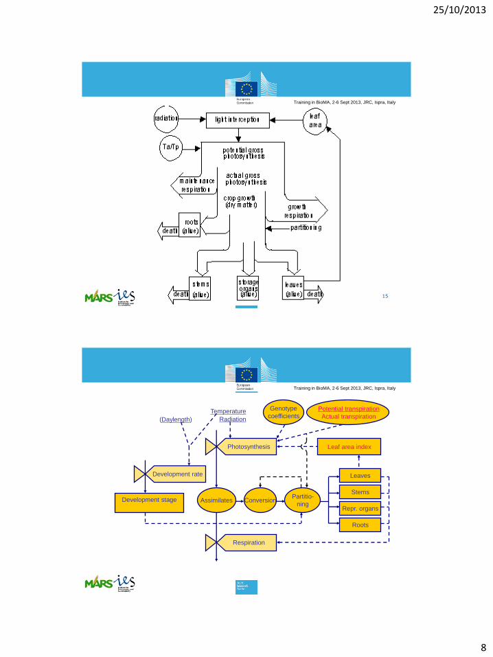
Photosynthesis
Respiration
Leaf area index
Genotype
coefficientsTemperature
Radiation
Assimilates ConversionPartitio-
ning
Leaves
Stems
Repr. organs
Roots
Development rate
Development stage
(Daylength)
Potential transpiration
Actual transpiration
25/10/2013
9
Training in BioMA, 2-6 Sept 2013, JRC, Ispra, Italy
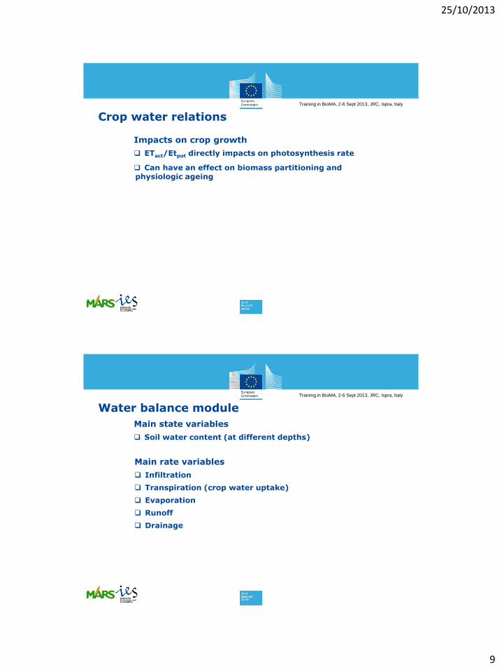
Crop water relations
Impacts on crop growth
ETact/Etpot directly impacts on photosynthesis rate
Can have an effect on biomass partitioning and physiologic ageing
Training in BioMA, 2-6 Sept 2013, JRC, Ispra, Italy
Water balance module
Main state variables
Soil water content (at different depths)
Main rate variables
Infiltration
Transpiration (crop water uptake)
Evaporation
Runoff
Drainage
25/10/2013
10
Training in BioMA, 2-6 Sept 2013, JRC, Ispra, Italy
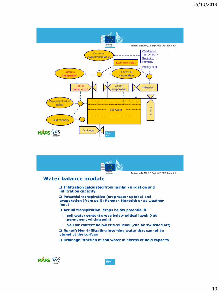
Windspeed
Temperature
Radiation
Humidity
Potential
evapotranspiration
Actual
transpiration
Actual
evaporation
Drainage
Soil water
Potential
evaporation
Infiltration
Runoff
Field capacity
Permanent wilting
point
Potential
transpiration
Leaf area index
Precipitation
Training in BioMA, 2-6 Sept 2013, JRC, Ispra, Italy
Water balance module
Infiltration calculated from rainfall/irrigation and infiltration capacity
Potential transpiration (crop water uptake) and evaporation (from soil): Penman Monteith or as weather input
Actual transpiration: drops below potential if
• soil water content drops below critical level; 0 at permanent wilting point
• Soil air content below critical level (can be switched off)
Runoff: Non-infiltrating incoming water that cannot be stored at the surface
Drainage: fraction of soil water in excess of field capacity
25/10/2013
11
Training in BioMA, 2-6 Sept 2013, JRC, Ispra, Italy
Water balance module
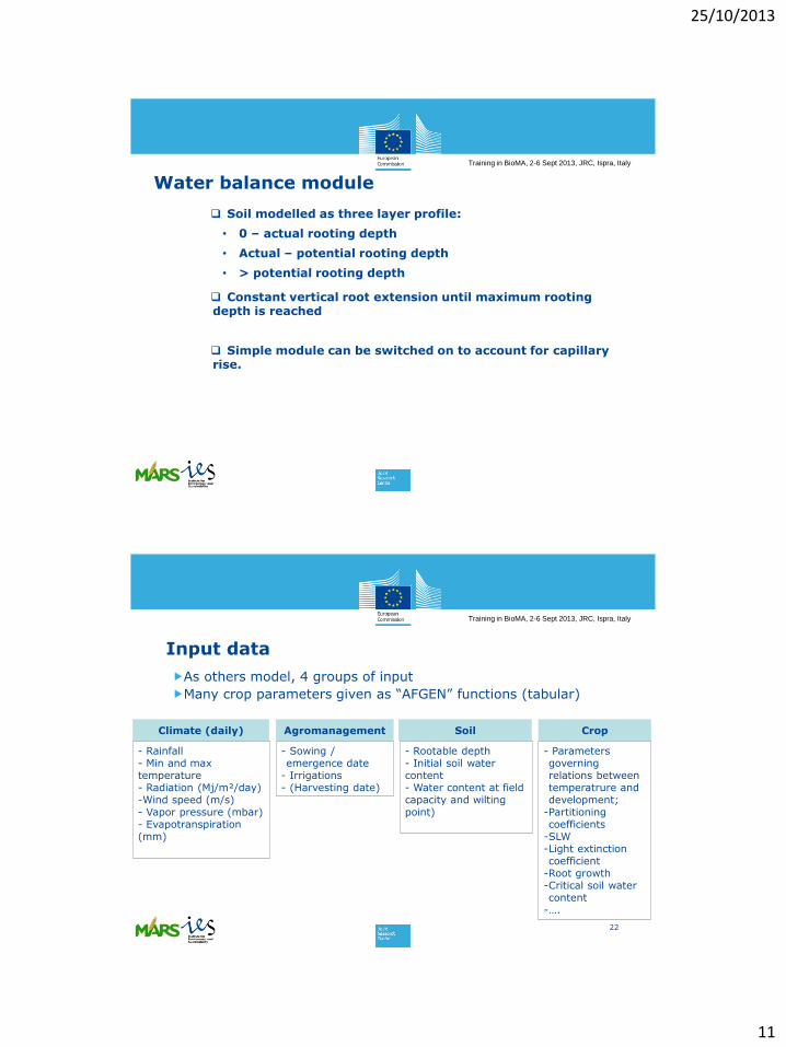
Soil modelled as three layer profile:
• 0 – actual rooting depth
• Actual – potential rooting depth
• > potential rooting depth
Constant vertical root extension until maximum rooting depth is reached
Simple module can be switched on to account for capillary rise.
Training in BioMA, 2-6 Sept 2013, JRC, Ispra, Italy
Input data
As others model, 4 groups of input
Many crop parameters given as “AFGEN” functions (tabular)
22
- Rainfall- Min and max temperature- Radiation (Mj/m²/day)-Wind speed (m/s)- Vapor pressure (mbar)- Evapotranspiration (mm)
- Sowing / emergence date
- Irrigations- (Harvesting date)
- Rootable depth- Initial soil water content- Water content at fieldcapacity and wiltingpoint)
- Parametersgoverningrelations betweentemperatrure and development;
-Partitioningcoefficients
-SLW-Light extinction coefficient
-Root growth-Critical soil water content
-….
Climate (daily) Agromanagement Soil Crop

25/10/2013
12
Training in BioMA, 2-6 Sept 2013, JRC, Ispra, Italy
Conclusions
23
Strengths:- Sophisticated calculation of photosynthesis and biomass
accumulation, based on universal principles- Model based on universal principles should make it universally
applicable and facilitate parameterization- Several decades of continued support and development (…)- Well documented
Weaknesses:- Several constants and fixed relations are not really constant- Afgen functions not elegant- Water balance (and soil in general) strongly simplified
compared to other model components- User community rather restricted- Lacks simulation of nutrients, pests etc- Lacks management options
25/10/2013
1
WARM model:overview and applications
Simone Bregaglio and Giovanni Cappelli
On behalf of the development team
University of Milan, CASSANDRA (Centre for Advanced Simulation Studies AND Researches on Agroecological modelling), [email protected]
BASAL project training course – JRC Ispra, Italy – 03 September 2013
BASAL project training course – JRC Ispra, Italy – 03 September 2013
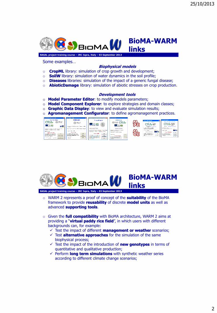
BioMA-WARMlinks
o WARM 2 is a component-based application developed following the same software architecture of BioMA.
o The same software components implemented in many BioMAmodelling solutions are re-used and implemented in WARM 2.
o Not only algorithms, also development tools are used in WARM 2 application.
25/10/2013
2
BASAL project training course – JRC Ispra, Italy – 03 September 2013
Some examples…Biophysical models
o CropML library: simulation of crop growth and development;o SoilW library: simulation of water dynamics in the soil profile;o Diseases libraries: simulation of the impact of a generic fungal disease;o AbioticDamage library: simulation of abiotic stresses on crop production.
Development toolso Model Parameter Editor: to modify models parameters;o Model Component Explorer: to explore strategies and domain classes;o Graphic Data Display: to view and evaluate simulation results;o Agromanagement Configurator: to define agromanagement practices.
BioMA-WARMlinks
BASAL project training course – JRC Ispra, Italy – 03 September 2013
o WARM 2 represents a proof of concept of the suitability of the BioMAframework to provide reusability of discrete model units as well as advanced supporting tools.
o Given the full compatibility with BioMA architecture, WARM 2 aims at providing a “virtual paddy rice field”, in which users with different backgrounds can, for example: Test the impact of different management or weather scenarios; Test alternative approaches for the simulation of the same
biophysical process; Test the impact of the introduction of new genotypes in terms of
quantitative and qualitative production; Perform long term simulations with synthetic weather series
according to different climate change scenarios;
BioMA-WARMlinks
25/10/2013
3
BASAL project training course – JRC Ispra, Italy – 03 September 2013
Outline
Introduction
Description of key processes
Application results
Conclusions
The practical exercise
BASAL project training course – JRC Ispra, Italy – 03 September 2013
Outline
Introduction
Description of key processes
Application results
Conclusions
The practical exercise

25/10/2013
4
BASAL project training course – JRC Ispra, Italy – 03 September 2013
Introduction
Given the paramount importance of rice crop as a staple food at a global level, many crop simulators were developed specifically to reproduce the peculiarities of paddy rice agricultural systems.
As an example, AgMIP rice team is composed by 13 rice models (e.g., Oryza2000, CERES-rice, DNDC-Rice, RiceGrow, GEMRICE).
Why another rice crop model?
Many aspects strongly affecting rice yields in temperate climate are not properly considered by existing approaches, like:o floodwater effect on vertical thermal profile;o spikelet sterility due to pre-flowering temperature shocks;o blast disease;o peculiar hydrology of paddy rice when soil presents high hydraulic
conductivity;o grain quality characteristics.
BASAL project training course – JRC Ispra, Italy – 03 September 2013
Introduction
The development of WARM (Water Accounting Rice Model) started in 2005, aiming at a model:
o able to take into account all the key processes affecting rice crop quantitative and qualitative productions (biotic and abiotic stresses, grain composition, micrometeorology);
o presenting a balance between the level of detail adopted to reproduce the biophysical processes related to crop growth and development (e.g., phenology, biomass accumulation, assimilate partitioning)
o showing a marked usability, in terms of intuitiveness of the graphical user interface and of capability of setting up a customized modelling solution, according to the user needs.

25/10/2013
5
BASAL project training course – JRC Ispra, Italy – 03 September 2013
Outline
Introduction
Description of key processes
Application results
Conclusions
The practical exercise
BASAL project training course – JRC Ispra, Italy – 03 September 2013
Time step:
o The simplification of using daily temperatures holds only when almost all the corresponding hourly temperatures fall within the range the crop is adapted to;
o If hourly temperatures in the warmest or coldest hours of the day are outside that range, the use of average daily temperature would lead to errors in the estimation of the temperature effect on photosynthesisand accumulation of thermal time;
o for sure the use of daily temperatures is a simplification that proved to work, at least under conditions the crop is adapted to but we need to consider scenarios for which the crop could be less adapted (climate change issues, new environments)
Development & growth

25/10/2013
6
Time step:
Tn
DayDay length = 12; Tmin = 24; Tmax = 43; Tavg=33.5
Crop Tn = 12;Tx = 43; To= 33;
To
Tx
BASAL project training course – JRC Ispra, Italy – 03 September 2013
Development & growth
BASAL project training course – JRC Ispra, Italy – 03 September 2013
Tn
To
Tx
Tn
To
Tx
f(t) = 0.998hour T (°C) f(t)
8 31.04 0.969
9 33.50 0.998
10 35.96 0.913
11 38.25 0.701
12 40.22 0.395
13 41.73 0.068
14 42.68 0.000
15 43.00 0.000
16 42.68 0.000
17 41.73 0.068
18 40.22 0.395
19 38.25 0.701
20 35.96 0.913
f(t) avg = 0.471
DAILY TIME STEP
HOURLY TIME STEP
Tavg=33.5 °C
Development & growth
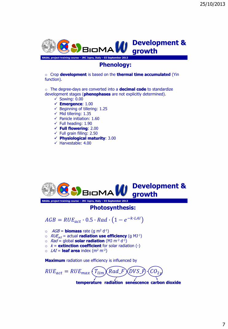
25/10/2013
7
BASAL project training course – JRC Ispra, Italy – 03 September 2013
Development & growth
Phenology:
o Crop development is based on the thermal time accumulated (Yin function).
o The degree-days are converted into a decimal code to standardize development stages (phenophases are not explicitly determined).
Sowing: 0.00 Emergence: 1.00 Beginning of tillering: 1.25 Mid tillering: 1.35 Panicle initiation: 1.60 Full heading: 1.90 Full flowering: 2.00 Full grain filling: 2.50 Physiological maturity: 3.00 Harvestable: 4.00
BASAL project training course – JRC Ispra, Italy – 03 September 2013
Development & growth
Photosynthesis:
𝐴𝐺𝐵 = 𝑅𝑈𝐸𝑎𝑐𝑡 ∙ 0.5 ∙ 𝑅𝑎𝑑 ∙ 1 − 𝑒−𝑘∙𝐿𝐴𝐼
o AGB = biomass rate (g m2 d-1)o RUEact = actual radiation use efficiency (g MJ-1)o Rad = global solar radiation (MJ m-2 d-1)o k = extinction coefficient for solar radiation (-)o LAI = leaf area index (m2 m-2)
Maximum radiation use efficiency is influenced by
𝑅𝑈𝐸𝑎𝑐𝑡 = 𝑅𝑈𝐸𝑚𝑎𝑥 ∙ 𝑇𝑙𝑖𝑚 ∙ 𝑅𝑎𝑑_𝐹 ∙ 𝐷𝑉𝑆_𝐹 ∙ 𝐶𝑂2𝐹
temperature radiation senescence carbon dioxide

25/10/2013
8
BASAL project training course – JRC Ispra, Italy – 03 September 2013
Development & growth
Partitioning of assimilates is driven by a single parameter, i.e., the fraction of photosynthates allocated to leaves at emergence.
1 1.7 2 2.5 3
BASAL project training course – JRC Ispra, Italy – 03 September 2013
Development & growth
Leaf area evolution:
o Specific leaf area (m2 kg-1) varies from sowing to tillering. o Leaf area index (LAI) increment is the product of SLA and the rate of aboveground biomass partitioned to the leaves. o Senescence is computed by subtracting dead LAI to the total one. Eachday a LAI unit is emitted and a degree days threshold is assigned (leaf life)
1 1.35

25/10/2013
9
BASAL project training course – JRC Ispra, Italy – 03 September 2013
Micrometeosimulation
o Quantification of the effect of flooding water on development and growtho Temperature is one of the most relevant driving variables for crop modelso Uncertainties in its estimation decidedly lower the degree of adherenceof the model to the real system
0
5
10
15
20
25
30
35
minutes
Tem
pera
ture
(°C
)
0
5
10
15
20
25
30
Wate
r le
vel
(cm
)
air T (170cm; °C)
air T (20 cm; °C)
water T (°C)
water level (cm)
Close canopy stage
BASAL project training course – JRC Ispra, Italy – 03 September 2013
Soil hydrology
o UNIMI.SoilW component is linked to CropML component in order to simulate water dynamics in the soil profile;
o Soil can be divided in a variable number of layers of different thickness, each one with its properties (e.g., texture, hydraulic conductivity)
o Three levels of users were identified:
Expert: he/she directly composes – on the base of his/her experience and of the specific context – different simple strategies to build a complete model
Intermediate user: he/she can chooses composite strategies implementing different complete models (e.g., EPIC, CropSyst, CERES)
Beginner (or expert in other sub-domains): it is possible to select a context strategy: the component autonomously select the configuration of hydrological model more suitable for the conditions explored (e.g., availability of data)

25/10/2013
10
Is Lambda (water extraction parameter) available?
Yes
No
Is water potential at leaf wilting available?
Yes
No

25/10/2013
11
SoilW
Is Lambda (water extraction parameter) available?
Yes
No
Is water potential at leaf wilting available?
Yes
No
SoilW
Is Lambda (water extraction parameter) available?
Yes
No
Is water potential at leaf wilting available?
Yes
No
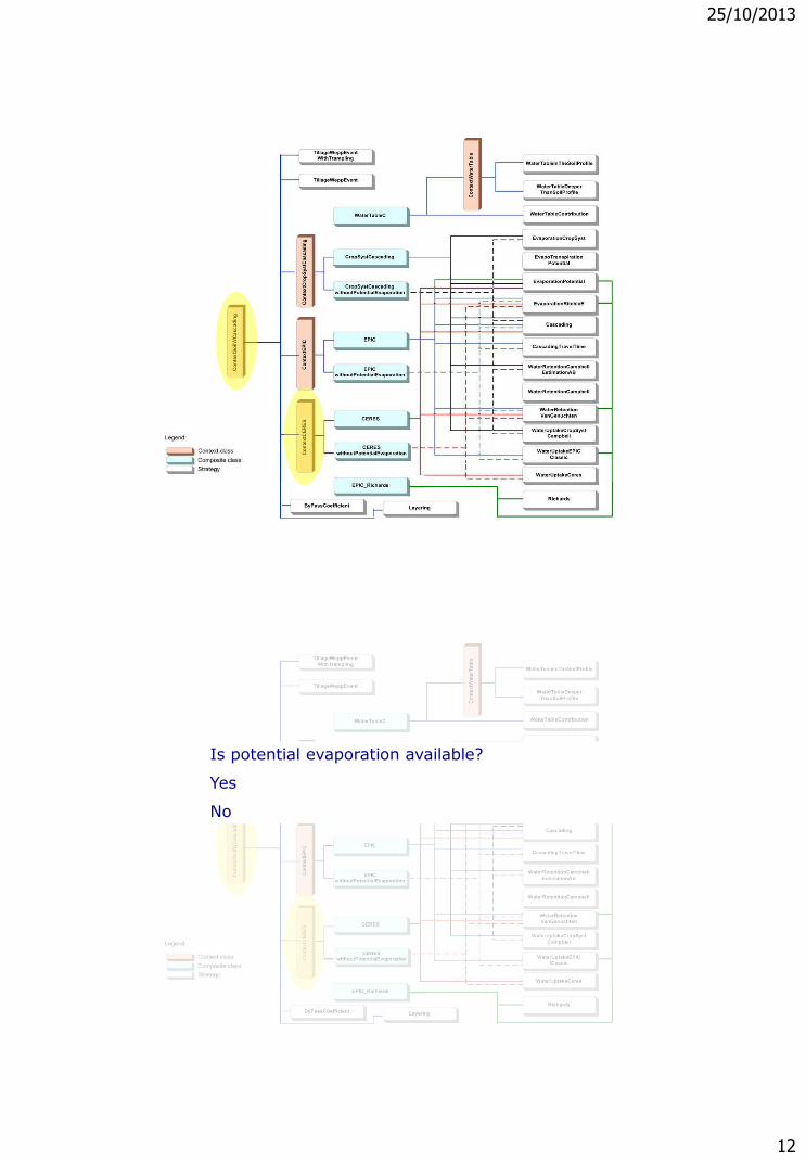
25/10/2013
12
SoilW
Is potential evaporation available?
Yes
No
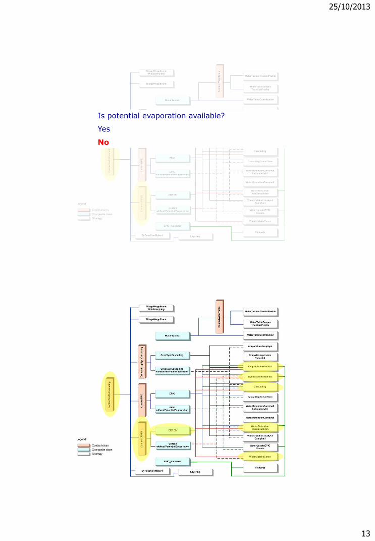
25/10/2013
13
SoilW
Is potential evaporation available?
Yes
No
SoilW

25/10/2013
14
BASAL project training course – JRC Ispra, Italy – 03 September 2013
Abiotic stresses:spikelet sterility
o The frequency of extreme events is expected to change (IPCC, 2007)o Temperature related shocks will surely change their impact, with different effects in different areas
BASAL project training course – JRC Ispra, Italy – 03 September 2013
Abiotic stresses:spikelet sterility
headDay
headDayi
GDDGDD
h
hid
i
eTTSterility22
224
1
,
2
211
2
1
Fattore campana
Fattori orariHourly factors Bell factorTime (hours)
T (°C)
sterilitythreshold
0
0.2
0.4
0.6
0.8
1
497 597 697 797 897 997 1097
Developing stage (GDD)
bell
facto
r
high bell factor
low bell factor
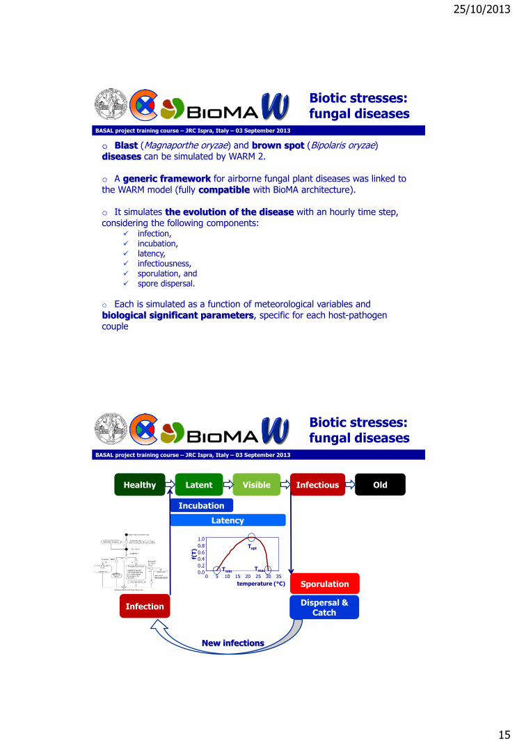
25/10/2013
15
BASAL project training course – JRC Ispra, Italy – 03 September 2013
Biotic stresses:fungal diseases
o Blast (Magnaporthe oryzae) and brown spot (Bipolaris oryzae)diseases can be simulated by WARM 2.
o A generic framework for airborne fungal plant diseases was linked to the WARM model (fully compatible with BioMA architecture).
o It simulates the evolution of the disease with an hourly time step, considering the following components:
infection, incubation, latency, infectiousness, sporulation, and spore dispersal.
o Each is simulated as a function of meteorological variables and biological significant parameters, specific for each host-pathogen couple
Biotic stresses:fungal diseases
0.0
0.2
0.4
0.6
0.8
1.0
0 5 10 15 20 25 30 35
temperature (°C)
f(T
)
Topt
TminTmax
Healthy OldVisible InfectiousLatent
Incubation
Latency
Infection
Sporulation
Dispersal &Catch
New infections
BASAL project training course – JRC Ispra, Italy – 03 September 2013

25/10/2013
16
BASAL project training course – JRC Ispra, Italy – 03 September 2013
Biotic stresses:fungal diseases
BASAL project training course – JRC Ispra, Italy – 03 September 2013
Grain quality
o Process-based models are used to forecast the potential impacts of climate change on agricultural systems and to define adaptation strategies (White et al., 2011).
o Crop quality represents an aspect scarcely investigated in crop modelling activities (Porter et al., 2005), but is fundamental to assess: the economic and nutritional value (Koutroubas et al., 2004); food security levels.
o Many authors agree in forecasting a decay in crop quality underclimate change conditions (Oury et al., 2003; Erda et al., 2005; Porter et al., 2005;
Slingo et al., 2005; Terao et al., 2005; Da Matta et al., 2010; Yamakawa et al., 2010; Okada et al, 2011;Shah et al., 2011; Wanga et al., 2011; Fernando et al., 2012; Madan et al., 2012; Ning et al., 2012;Weigel et al., 2012; Högi et al., 2013 ).
o Superior grain quality of rice has become a key target in current riceproduction (Cheng and Zhu, 1998; Huang et al., 1998; Li et al., 2005; Tesio et al.,
2013).
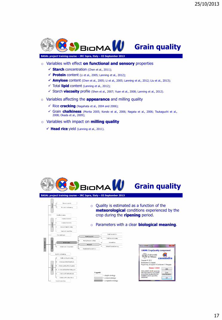
25/10/2013
17
BASAL project training course – JRC Ispra, Italy – 03 September 2013
Grain quality
o Variables with effect on functional and sensory properties
o Variables affecting the appearance and milling quality
o Variables with impact on milling quality
Starch concentration (Chen et al., 2011);
Protein content (Li et al., 2005; Lanning et al., 2012);
Amylose content (Chen et al., 2005; Li et al., 2005; Lanning et al., 2012; Liu et al., 2013);
Total lipid content (Lanning et al., 2012);
Starch viscosity profile (Shen et al., 2007; Yuan et al., 2008; Lanning et al., 2012).
Rice cracking (Nagahata et al., 2004 and 2006);
Grain chalkiness (Morita 2005; Kondo et al., 2006; Nagata et al., 2006; Tsukaguchi et al.,
2008; Okada et al., 2009);
Head rice yield (Lanning et al., 2011).
BASAL project training course – JRC Ispra, Italy – 03 September 2013
Grain quality
o Quality is estimated as a function of the meteorological conditions experienced by the crop during the ripening period.
o Parameters with a clear biological meaning.
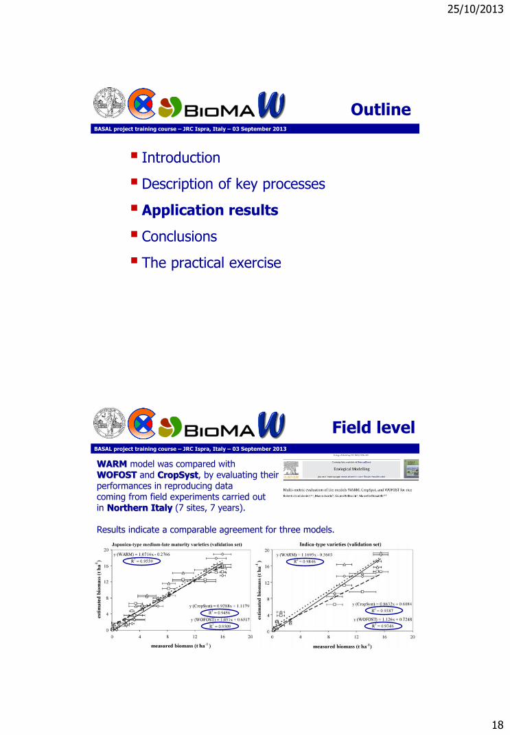
25/10/2013
18
BASAL project training course – JRC Ispra, Italy – 03 September 2013
Outline
Introduction
Description of key processes
Application results
Conclusions
The practical exercise
BASAL project training course – JRC Ispra, Italy – 03 September 2013
Field level
WARM model was compared with WOFOST and CropSyst, by evaluating theirperformances in reproducing data coming from field experiments carried outin Northern Italy (7 sites, 7 years).
Results indicate a comparable agreement for three models.

25/10/2013
19
BASAL project training course – JRC Ispra, Italy – 03 September 2013
Yieldforecasting
o The availability of operational monitoring systems is crucial to provide objective, timely and quantitative yield forecasts at regional and national scale;
o Most of the existing crop yield forecasting systems have been developed by coupling crop models with weather and soil databases in order to perform large-area simulations under potential and, in some cases, water limiting conditions.
o WARM model is used since years by the European Commission to forecast rice productions at EU 27 level;
o It was also applied to countries that play a major role in crop production at world level like China and India, and recently in Senegal, which is the 10th rice importer country, whose Government is pushing towards self-sufficiency.
BASAL project training course – JRC Ispra, Italy – 03 September 2013
Yieldforecasting
o To develop an effective crop yield forecasting system, three main points have to be considered: the need of the customer/user (European Commission, insurance
company); the spatial and temporal resolution of the forecast; the conditions of application (information available, agroclimatic
conditions)
26/09/200801/08/2008
o Rice yield forecasts at EU level consider the impact on crop production of spikelet sterility; blast disease
o Yield forecasts are updated during the growing season
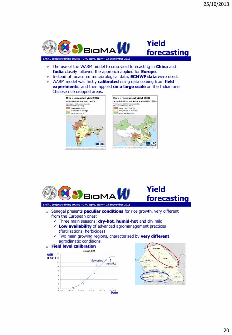
25/10/2013
20
BASAL project training course – JRC Ispra, Italy – 03 September 2013
Yieldforecasting
o The use of the WARM model to crop yield forecasting in China and India closely followed the approach applied for Europe.
o Instead of measured meteorological data, ECMWF data were used. o WARM model was firstly calibrated using data coming from field
experiments, and then applied on a large scale on the Indian and Chinese rice cropped areas.
BASAL project training course – JRC Ispra, Italy – 03 September 2013
Yieldforecasting
o Senegal presents peculiar conditions for rice growth, very different from the European ones: Three main seasons: dry-hot, humid-hot and dry mild Low availability of advanced agromanagement practices
(fertilizations, herbicides) Two main growing regions, characterized by very different
agroclimatic conditionso Field level calibration
floweringmaturity
Date
AGB(t ha-1)

25/10/2013
21
BASAL project training course – JRC Ispra, Italy – 03 September 2013
Yieldforecasting
o The system includes the simulation of biotic and abiotic stresses; the assimilation of remotely sensed data
to determine sowing dates; as regressors to forecast yields.
o The elementary simulation unit is the 25 × 25 km cell of the grid weather (ECMWF data)
o Tests performed with multiple regressions with indicators from the first decade after maturity
o Different tests were performed, e.g., potential growth – model not calibrated – fixed sowing dates; biotic and abiotic limitation – model calibrated – fixed sowing dates biotic and abiotic limitation – model calibrated – variable sowing dates
R2 = 0.88 (R2 trend: 0.68)
Indicators:• Biomass• LAI• Storage organs• DVS
R2 = 0.96 (R2 trend: 0.68)
Indicators:• Blast infection events• Blast-LAI• Blast-storage organs• Brown spot infection events
BASAL project training course – JRC Ispra, Italy – 03 September 2013
Yieldforecasting

25/10/2013
22
BASAL project training course – JRC Ispra, Italy – 03 September 2013
Yieldforecasting
R2 = 0.96 (R2 trend: 0.68)
Indicators:• Biomass• LAI• Storage organs• DVS
R2 = 0.98 (R2 trend: 0.68)
Indicators:• Storage organs• DVS• LAI• Heat induced sterility
BASAL project training course – JRC Ispra, Italy – 03 September 2013
Continentalscale
The same modelling solution implemented in WARM 2 was used at continental scale to assess the impact of climate change on South America and Caribbean.
Simulations were performed by considering the implementation of adaptationstrategies (modification of the length of the crop cycle and shift in the sowing dates).
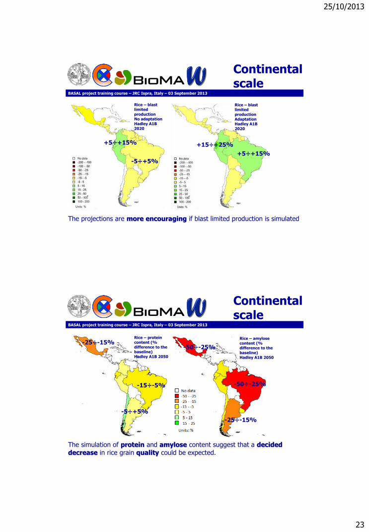
25/10/2013
23
BASAL project training course – JRC Ispra, Italy – 03 September 2013
Continentalscale
In 2020 the model forecasts an increase in rice potential production in Latin America even without adaptation strategiesThe projections are more encouraging if blast limited production is simulated
Rice –potentialproductionNo adaptationHadley A1B 2020
Rice –potentialproductionAdaptation Hadley A1B 2020
-15÷-5%
+5÷+15%+5÷+15%
-5÷+5%
-5÷+5%
Rice – blastlimitedproductionNo adaptationHadley A1B 2020
Rice – blastlimitedproductionAdaptationHadley A1B 2020
-5÷+5%
+5÷+15%
+5÷+15%
+15÷+25%
BASAL project training course – JRC Ispra, Italy – 03 September 2013
Continentalscale
The simulation of protein and amylose content suggest that a decided decrease in rice grain quality could be expected.
-15÷-5%
-25÷-15%
-5÷+5%
Rice – proteincontent (% difference to the baseline)Hadley A1B 2050
Rice – amylosecontent (% difference to the baseline)Hadley A1B 2050
-25÷-15%
-50÷-25%
-50÷-25%

25/10/2013
24
BASAL project training course – JRC Ispra, Italy – 03 September 2013
In silicoideotyping
o Crop simulation models were developed aiming at two specific objectives:
Studying production enterprises, to maximize yields while optimizingthe use of resources, and
Studying genotype × environment interactions, as a tool to support variety selection and improvement. How is it possible?
2. Crop growth and development are simulated as a function of meteorologicaland agromanagementinputs.
1. Crop morpho-physiologicalfeatures are reproduced via model parameters.
BASAL project training course – JRC Ispra, Italy – 03 September 2013
In silicoideotyping
In Silico Ideotyping platform
ISIde1. Select the rice district 2. Develop the ideotype
3. Select weather scenario 4. View/export the results
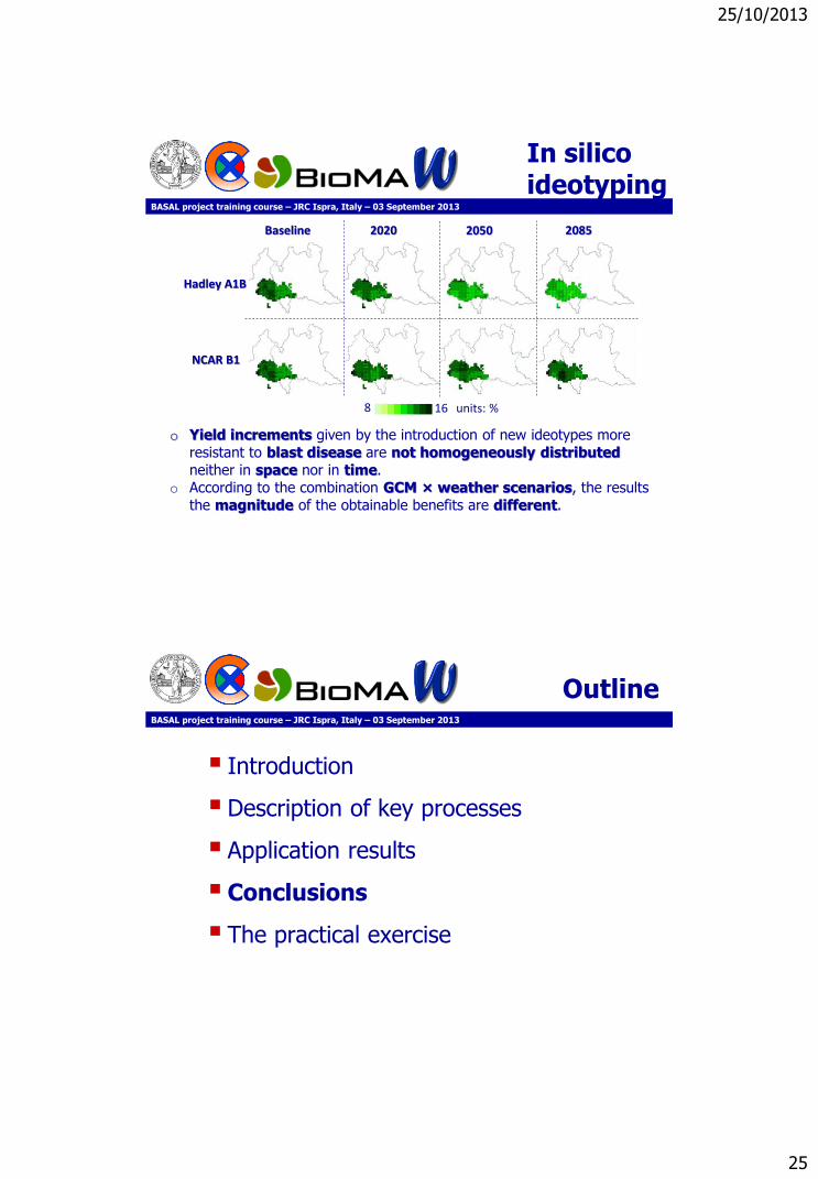
25/10/2013
25
BASAL project training course – JRC Ispra, Italy – 03 September 2013
In silicoideotyping
o Yield increments given by the introduction of new ideotypes more resistant to blast disease are not homogeneously distributed neither in space nor in time.
o According to the combination GCM × weather scenarios, the results the magnitude of the obtainable benefits are different.
Hadley A1B
NCAR B1
Baseline 2020 2050 2085
8 16 units: %
BASAL project training course – JRC Ispra, Italy – 03 September 2013
Outline
Introduction
Description of key processes
Application results
Conclusions
The practical exercise

25/10/2013
26
BASAL project training course – JRC Ispra, Italy – 03 September 2013
Conclusions
o A software component able to simulate soil carbon and nitrogen dynamics in paddy rice fields is under development.
o This component will be linked to WARM 2 modelling solution and will allow to simulate the impacts of agro-management practices on crop growth.
o It will simulate the processes leading to gas emission: aerobic and anaerobic respiration; nitrification and denitrification; methanogenesis; ammonia volatilization.
o A requisite of this component is the balancebetween the detail adopted in the formalization of modelling approaches and the need in terms of inputavailability.
BASAL project training course – JRC Ispra, Italy – 03 September 2013
Conclusions
Thanks to the software architecture shared with BioMA, the WARM 2 modelling solution can be used to multiple purposes and spatial scales.
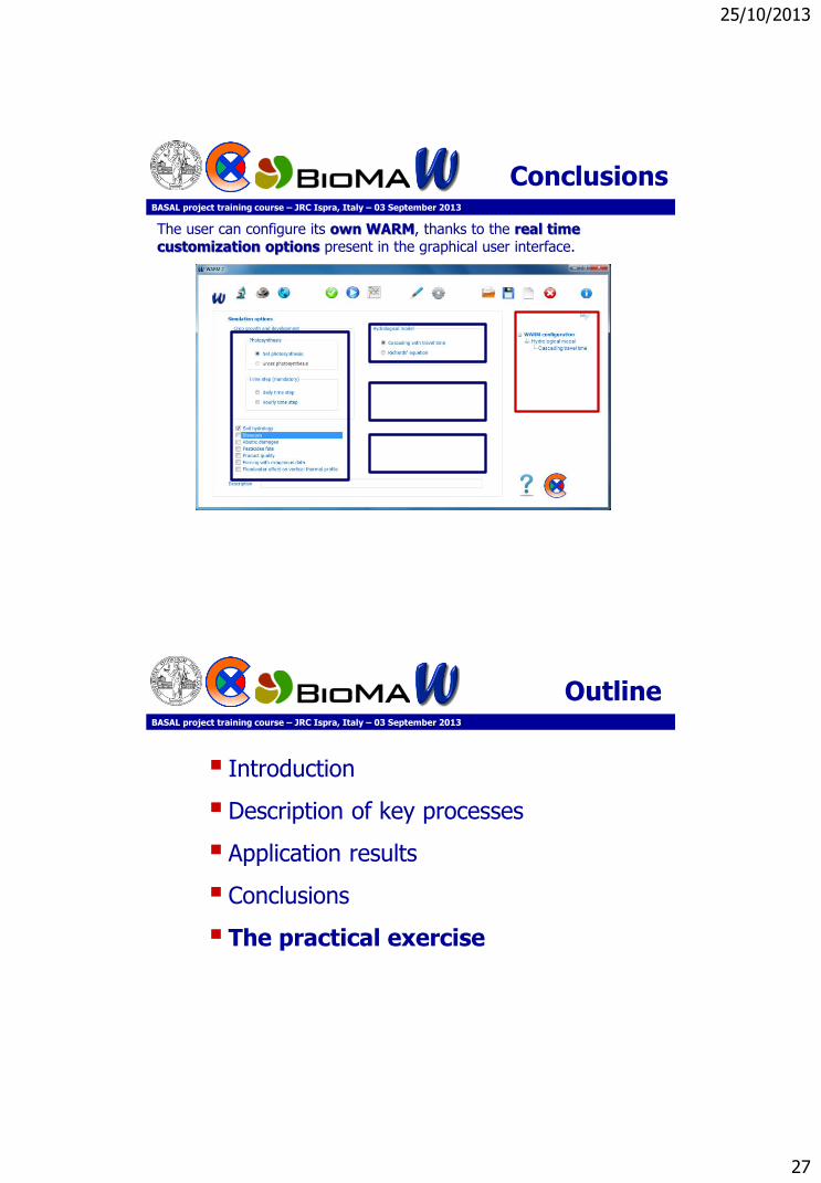
25/10/2013
27
BASAL project training course – JRC Ispra, Italy – 03 September 2013
Conclusions
The user can configure its own WARM, thanks to the real time customization options present in the graphical user interface.
BASAL project training course – JRC Ispra, Italy – 03 September 2013
Outline
Introduction
Description of key processes
Application results
Conclusions
The practical exercise
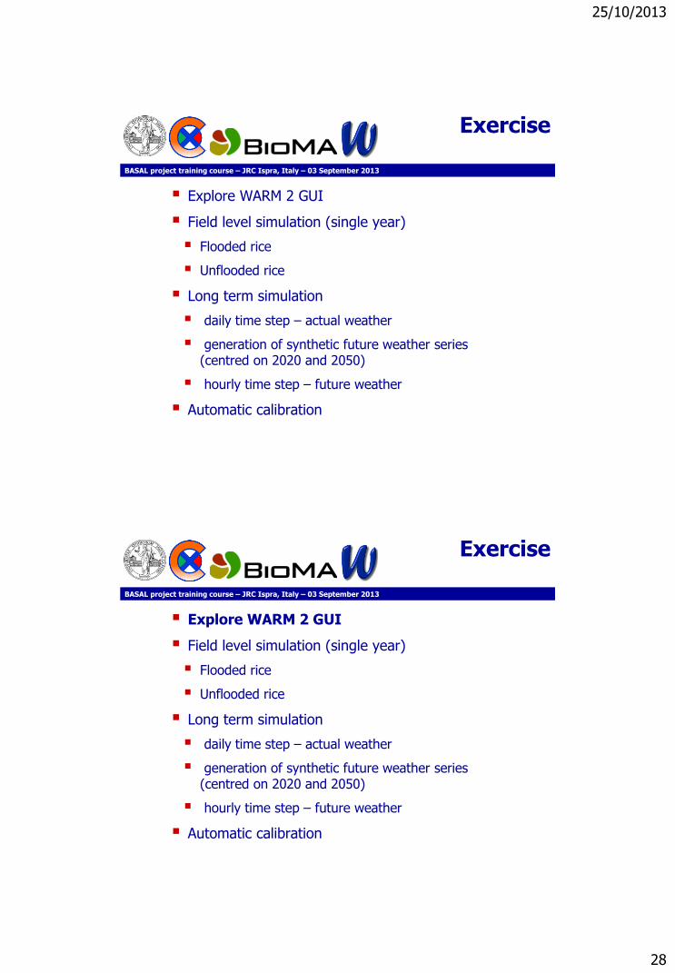
25/10/2013
28
BASAL project training course – JRC Ispra, Italy – 03 September 2013
Exercise
Explore WARM 2 GUI
Field level simulation (single year)
Flooded rice
Unflooded rice
Long term simulation
daily time step – actual weather
generation of synthetic future weather series(centred on 2020 and 2050)
hourly time step – future weather
Automatic calibration
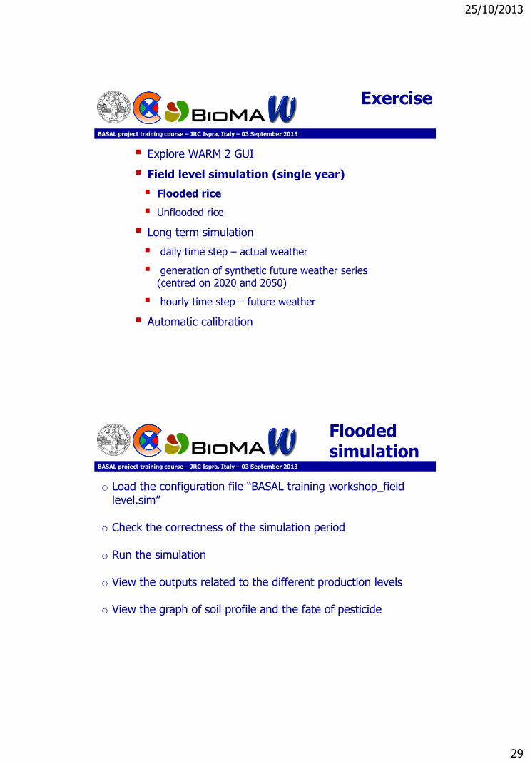
25/10/2013
29
BASAL project training course – JRC Ispra, Italy – 03 September 2013
Exercise
Explore WARM 2 GUI
Field level simulation (single year)
Flooded rice
Unflooded rice
Long term simulation
daily time step – actual weather
generation of synthetic future weather series(centred on 2020 and 2050)
hourly time step – future weather
Automatic calibration
BASAL project training course – JRC Ispra, Italy – 03 September 2013
Floodedsimulation
o Load the configuration file “BASAL training workshop_fieldlevel.sim”
o Check the correctness of the simulation period
o Run the simulation
o View the outputs related to the different production levels
o View the graph of soil profile and the fate of pesticide

25/10/2013
30
BASAL project training course – JRC Ispra, Italy – 03 September 2013
Exercise
Explore WARM 2 GUI
Field level simulation (single year)
Flooded rice
Unflooded rice
Long term simulation
daily time step – actual weather
generation of synthetic future weather series(centred on 2020 and 2050)
hourly time step – future weather
Automatic calibration
BASAL project training course – JRC Ispra, Italy – 03 September 2013
Unfloodedsimulation
o Build a new agromanagement file from the graphical user interface: Sowing: fixed date 121 DOY Chemical treatment:
fixed date 140 DOY Tricyclazolo, amount 200 g ha-1, fraction 0.5)
Harvest: fixed date 320 DOY. Then click on
o Save and view it with the Agromanagement Configuration Generator
o Validate and run the simulation
o View the graph of soil profile and the fate of pesticide
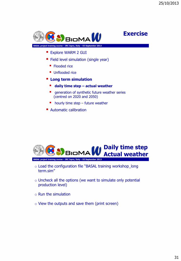
25/10/2013
31
BASAL project training course – JRC Ispra, Italy – 03 September 2013
Exercise
Explore WARM 2 GUI
Field level simulation (single year)
Flooded rice
Unflooded rice
Long term simulation
daily time step – actual weather
generation of synthetic future weather series(centred on 2020 and 2050)
hourly time step – future weather
Automatic calibration
BASAL project training course – JRC Ispra, Italy – 03 September 2013
Daily time stepActual weather
o Load the configuration file “BASAL training workshop_longterm.sim”
o Uncheck all the options (we want to simulate only potential production level)
o Run the simulation
o View the outputs and save them (print screen)
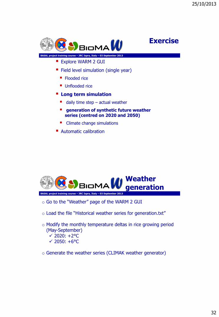
25/10/2013
32
BASAL project training course – JRC Ispra, Italy – 03 September 2013
Exercise
Explore WARM 2 GUI
Field level simulation (single year)
Flooded rice
Unflooded rice
Long term simulation
daily time step – actual weather
generation of synthetic future weatherseries (centred on 2020 and 2050)
Climate change simulations
Automatic calibration
BASAL project training course – JRC Ispra, Italy – 03 September 2013
Weathergeneration
o Go to the “Weather” page of the WARM 2 GUI
o Load the file “Historical weather series for generation.txt”
o Modify the monthly temperature deltas in rice growing period (May-September) 2020: +2°C 2050: +6°C
o Generate the weather series (CLIMAK weather generator)
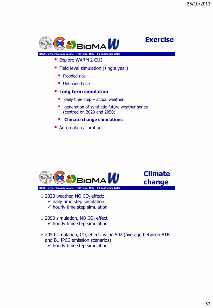
25/10/2013
33
BASAL project training course – JRC Ispra, Italy – 03 September 2013
Exercise
Explore WARM 2 GUI
Field level simulation (single year)
Flooded rice
Unflooded rice
Long term simulation
daily time step – actual weather
generation of synthetic future weather series(centred on 2020 and 2050)
Climate change simulations
Automatic calibration
BASAL project training course – JRC Ispra, Italy – 03 September 2013
Climatechange
o 2020 weather, NO CO2 effect: daily time step simulation hourly time step simulation
o 2050 simulation, NO CO2 effect hourly time step simulation
o 2050 simulation, CO2 effect. Value 502 (average between A1B and B1 IPCC emission scenarios) hourly time step simulation

25/10/2013
34
BASAL project training course – JRC Ispra, Italy – 03 September 2013
DailyActual weather
BASAL project training course – JRC Ispra, Italy – 03 September 2013
Daily2020
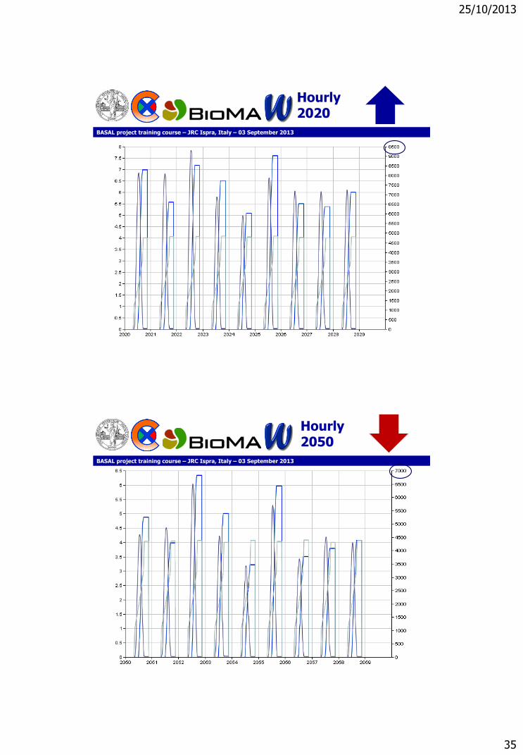
25/10/2013
35
BASAL project training course – JRC Ispra, Italy – 03 September 2013
Hourly2020
BASAL project training course – JRC Ispra, Italy – 03 September 2013
Hourly2050

25/10/2013
36
BASAL project training course – JRC Ispra, Italy – 03 September 2013
Hourly2050 CO2
BASAL project training course – JRC Ispra, Italy – 03 September 2013
Exercise
Explore WARM 2 GUI
Field level simulation (single year)
Flooded rice
Unflooded rice
Long term simulation
daily time step – actual weather
generation of synthetic future weather series(centred on 2020 and 2050)
Climate change simulations
Automatic calibration

10/25/2013
1
STICS – Principles of the model and implementation in Bioma
Remi Lecerf
125 October 2013
STICS
Stands for Simulateur mulTIdisciplinaire pour les Cultures Standard
(Multidisciplinary simulator of standard crops)
Developped by Agroclim Unit of INRA (Institut National de la
Recherche Agronomique)
http://www7.avignon.inra.fr/agroclim_stics
225 October 2013
10/25/2013
2
STICS
Main characteristics of the crop model:
Based on the Radiation Use Efficiency concept
Simulates a wide range of variables related to the crop and the
soil
Simulates water and nitrogen balance
Various plants can be simulated: Wheat, sugar beet, vineyard,
sugar cane, grasslands…
Possibility of simulating crop management practices
Daily simulations
STICS is based on empirical or semi-empirical relationships and is
inspired from other models
325 October 2013
STICS
1.Principles of the model and main components
2.Main differences with WOFOST
3.Interface of the model and data needed
4.Implementation of STICS in Bioma
5.Results of the first simulations of grasslands
425 October 2013
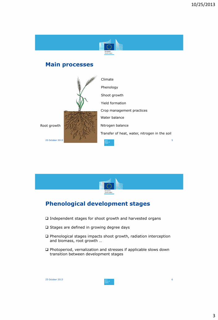
10/25/2013
3
Main processes
525 October 2013
Water balance
Nitrogen balance
Transfer of heat, water, nitrogen in the soil
Crop management practices
Climate
Phenology
Shoot growth
Yield formation
Root growth
Phenological development stages
625 October 2013
Independent stages for shoot growth and harvested organs
Stages are defined in growing degree days
Phenological stages impacts shoot growth, radiation interception and biomass, root growth …
Photoperiod, vernalization and stresses if applicable slows down transition between development stages

10/25/2013
4
Development stages
725 October 2013
Determinate crops:Vegetative and reproductive growth occur successively
Wheat, maize, barley, grasslands
Indeterminate cropsVegetative and reproductive growth occur simultaneously
(at least partially)Tomato, vineyards, sugar beet, sugar cane
Development stages
825 October 2013
10/25/2013
5
Leaf dynamics
925 October 2013
The daily Leaf Area Index (LAI) is determined by:
A logistic function driven by a normalized development unit and where leaf growth rate depends on phenological stages
A thermal function where high temperatures are favorable to leaf growth until a plant dependent threshold
A density function only active when plant density reaches a threshold
The combination of all stresses (water, nitrogen, waterlogging)
DELTAI = DELTAIDEV . DELTAIT . DELTAIDENS . DELTAISTRESS
Radiation Use efficiency
1025 October 2013
Two methods are used, depending on the crop
Homogenous crops The radiation intercepted by the plant is a simple function that depends on LAI and an extinction coefficient specific to the crop
Row crops A simplified radiative transfer model is used taking into account spacing between rows, height of the plant…The model compute the direct and diffuse part of radiation
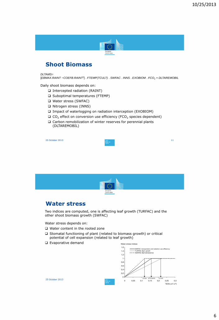
10/25/2013
6
Shoot Biomass
1125 October 2013
DLTAMS=
[EBMAX.RAINT −COEFB.RAINT2] . FTEMP(TCULT) . SWFAC . INNS . EXOBIOM . FCO2 + DLTAREMOBIL
Daily shoot biomass depends on:
Intercepted radiation (RAINT)
Suboptimal temperatures (FTEMP)
Water stress (SWFAC)
Nitrogen stress (INNS)
Impact of waterlogging on radiation interception (EXOBIOM)
CO2 effect on conversion use efficiency (FCO2 species dependent)
Carbon remobilization of winter reserves for perennial plants (DLTAREMOBIL)
Water stress
1225 October 2013
Two indices are computed, one is affecting leaf growth (TURFAC) and the other shoot biomass growth (SWFAC)
Water stress depends on:
Water content in the rooted zone
Stomatal functioning of plant (related to biomass growth) or critical potential of cell expansion (related to leaf growth)
Evaporative demand
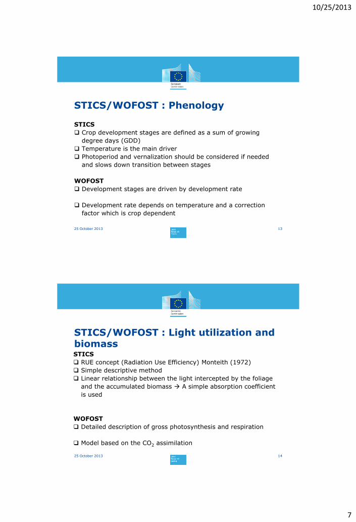
10/25/2013
7
STICS/WOFOST : Phenology
STICS
Crop development stages are defined as a sum of growing
degree days (GDD)
Temperature is the main driver
Photoperiod and vernalization should be considered if needed
and slows down transition between stages
WOFOST
Development stages are driven by development rate
Development rate depends on temperature and a correction
factor which is crop dependent
1325 October 2013
STICS/WOFOST : Light utilization and biomassSTICS
RUE concept (Radiation Use Efficiency) Monteith (1972)
Simple descriptive method
Linear relationship between the light intercepted by the foliage
and the accumulated biomass A simple absorption coefficient
is used
WOFOST
Detailed description of gross photosynthesis and respiration
Model based on the CO2 assimilation
1425 October 2013
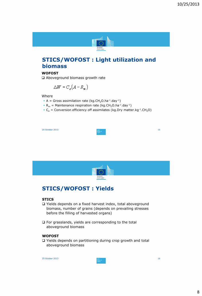
10/25/2013
8
STICS/WOFOST : Light utilization and biomassWOFOST
Aboveground biomass growth rate
Where
A = Gross assimilation rate (kg.CH2O.ha-1.day-1)
Rm = Maintenance respiration rate (kg.CH2O.ha-1.day-1)
Ce = Conversion efficiency off assimilates (kg.Dry matter.kg-1.CH2O)
1525 October 2013
STICS/WOFOST : Yields
STICS
Yields depends on a fixed harvest index, total aboveground
biomass, number of grains (depends on prevailing stresses
before the filling of harvested organs)
For grasslands, yields are corresponding to the total
aboveground biomass
WOFOST
Yields depends on partitioning during crop growth and total
aboveground biomass
1625 October 2013
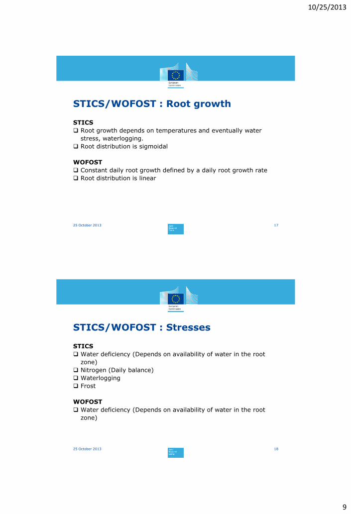
10/25/2013
9
STICS/WOFOST : Root growth
STICS
Root growth depends on temperatures and eventually water
stress, waterlogging.
Root distribution is sigmoidal
WOFOST
Constant daily root growth defined by a daily root growth rate
Root distribution is linear
1725 October 2013
STICS/WOFOST : Stresses
STICS
Water deficiency (Depends on availability of water in the root
zone)
Nitrogen (Daily balance)
Waterlogging
Frost
WOFOST
Water deficiency (Depends on availability of water in the root
zone)
1825 October 2013

10/25/2013
10
STICS/WOFOST : Climate and evapotranspiration
STICS
Crop temperature is computed instead of air temperature
Input evapotranspiration or calculated:
- Penman
- Priestley-Taylor
- Shuttleworth and Wallace
WOFOST
Penman evapotranspiration
1925 October 2013
STICS/WOFOST : Partitioning
STICS
The method is used for harvested organs in some cases, determinate
plants and annual plants. The size of the envelopes of harvested
organs is computed as a function of shoot growth
No partitioning for indeterminate plants and perennial plants
WOFOST
Roots, stems, leaves and storage organs are partitioned among the
shoot growth
Partitioning factors are crop specific and depends on development
stages
2025 October 2013

10/25/2013
11
STICS/WOFOST
STICS
Crop management practices (sowing, harvesting, irrigation) may
be simulated
Soil surface: Impact of mulch, impact of tillage on bulk density
Possibility to force the model with external data (field
measurements, satellite data)
2125 October 2013
Input data of the STICS modelAs others model, 4 groups of input
2225 October 2013
- Rainfall
- Min and max temperature
- Radiation (Mj/m²/day)
-Wind speed (m/s)
- Vapor pressure (mbar)
- Evapotranspiration (mm)
- Sowing
- Mowing
- Irrigations
- Fertilization
- Soil depth (5 horizons)
- Soil water content (Field
capacity and water content
at wilting point)
- Bulk density
- Organic nitrogen in the
soil
- Stone content
- Clay and limestone of the
surface
- Maximum depth or roots
- Development stages
(GDD)
- Threshold
temperatures
- Parameters related
to LAI growth
-….
Climate (daily) Agromanagement Soil Plant

10/25/2013
12
STICS interface
2325 October 2013
STICS implementation in Bioma
Actually the model is coupled with EPIC to simulate soil evaporation,
water content
The implementation is only suitable for grasslands simulation
Some part of the model are missing:
simulation cannot be started before emergence
frost is not taken into account
nitrogen balance is not implemented
partitioning is not implemented
Automatic crop management practices are not implemented
2425 October 2013

10/25/2013
13
STICS implementation in Bioma
2525 October 2013
Grasslands simulations over France
Simulation of temporary grasslands only
No agromanagement practices are considered
Yields are assumed to be equal to the aboveground biomass
produced throughout the year
Main drivers of yields formation are considered to be soils and
climate (through water balance and photoperiod)
2625 October 2013

10/25/2013
14
Grasslands simulations over France
On the period 1990-2012
2725 October 2013
Grasslands simulation over France
The soil is simulated with EPIC
The location of temporary grasslands may differ from reality
(problematic if we consider that soils are driving yields)
Agromanagement practices are not taken into account
Species are not considered (rye grass is cultivated in the west of
France whereas the species simulated simulated are similar to
orchard grass/fescue)
The definition of temporary grasslands may
2825 October 2013

10/25/2013
15
Example of validation at local scale
2925 October 2013
Results of simulations for 48
plots (southeastern France)
Irrigated grasslands with 3
mowing
Agromanagement practices
were collected by the farmer and
used as input
Conclusion and perspectives
3025 October 2013
The model implementation is still under development:
- Implementation of soil simulation
- Implementation of development stages before emergence
- Implementation of Nitrogen balance
In order to estimate grasslands yields:
- Providing suitable agromanagement practices for grasslands
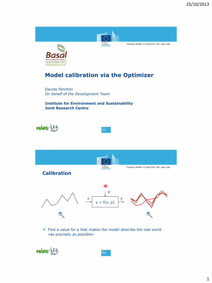
25/10/2013
1
Training in BioMA, 2-6 Sept 2013, JRC, Ispra, Italy
Model calibration via the Optimizer
Davide Fanchini
On behalf of the Development Team
Institute for Environment and Sustainability
Joint Research Centre
Training in BioMA, 2-6 Sept 2013, JRC, Ispra, Italy
Calibration
y = f(x, p)
p
x y
7642
Find a value for p that makes the model describe the real world
«as precisely as possible»
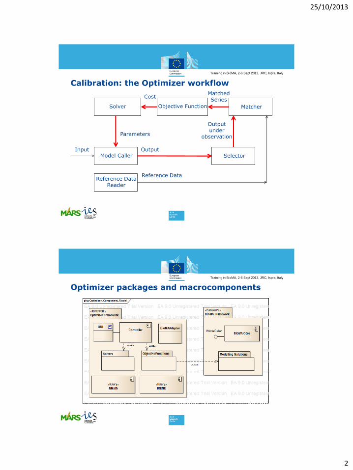
25/10/2013
2
Training in BioMA, 2-6 Sept 2013, JRC, Ispra, Italy
Calibration: the Optimizer workflow
Selector
Outputunder
observation
Matcher
MatchedSeries
Model Caller
Parameters
Input Output
Objective FunctionSolver
Cost
Reference DataReference Data
Reader
Training in BioMA, 2-6 Sept 2013, JRC, Ispra, Italy
Optimizer packages and macrocomponents
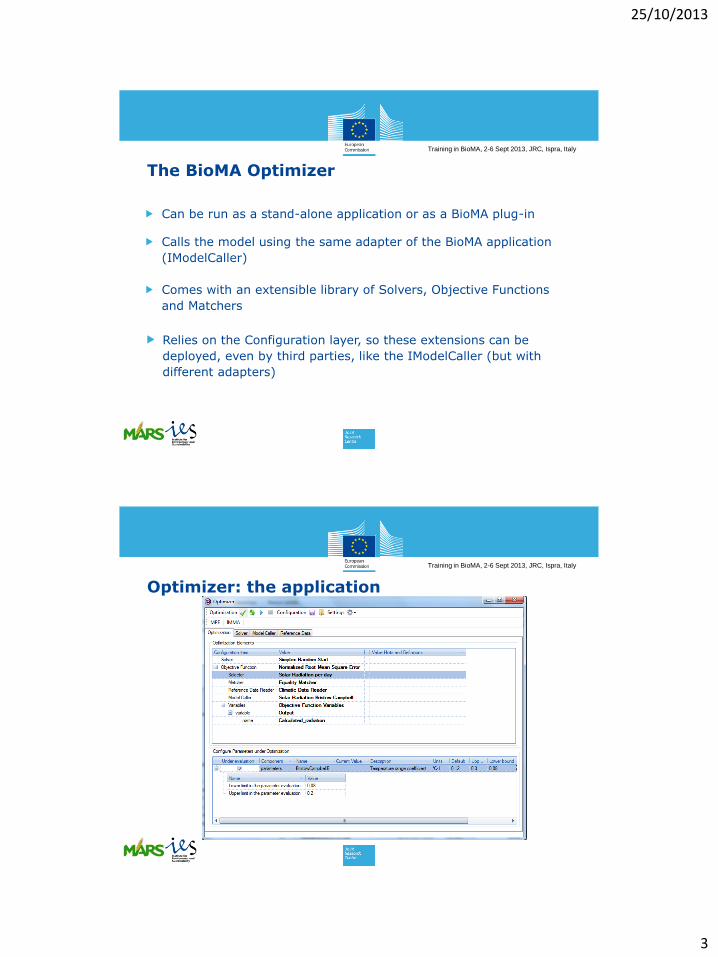
25/10/2013
3
Training in BioMA, 2-6 Sept 2013, JRC, Ispra, Italy
The BioMA Optimizer
Can be run as a stand-alone application or as a BioMA plug-in
Calls the model using the same adapter of the BioMA application
(IModelCaller)
Comes with an extensible library of Solvers, Objective Functions
and Matchers
Relies on the Configuration layer, so these extensions can be
deployed, even by third parties, like the IModelCaller (but with
different adapters)
Training in BioMA, 2-6 Sept 2013, JRC, Ispra, Italy
Optimizer: the application
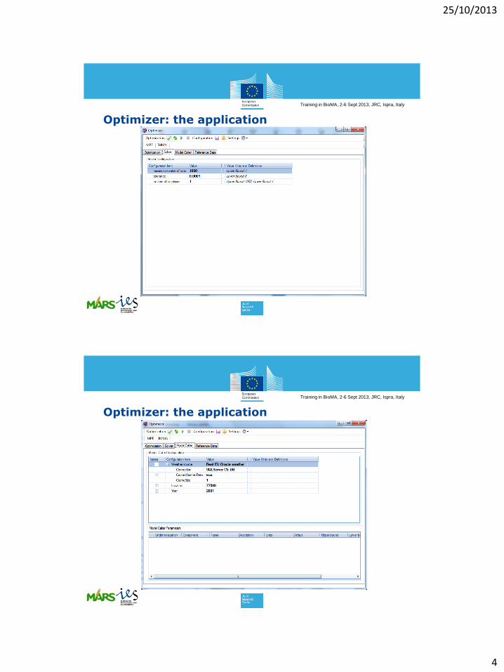
25/10/2013
4
Training in BioMA, 2-6 Sept 2013, JRC, Ispra, Italy
Optimizer: the application
Training in BioMA, 2-6 Sept 2013, JRC, Ispra, Italy
Optimizer: the application

25/10/2013
5
Training in BioMA, 2-6 Sept 2013, JRC, Ispra, Italy
Optimizer: the application
Training in BioMA, 2-6 Sept 2013, JRC, Ispra, Italy
Bristow&Campbell’s Solar Radiation Model
This model assumes a relationship between the range of daily
temperatures and the transmissivity of the atmosphere
TCSRADSRAD atmosphereoftopsurfaceearth Where TC is a transmissivity coefficient which varies from 0 to <1
averagemonthly
Tair
Tair
bCSTTC
2
exp1
Where CST is the clear sky transmissivity, and b an empirical
parameter
Problem: estimate the b parameter to minimize the difference
between predicted and measured values
One year of daily solar radiation data and air temperature data used