appendix a ghs—globally harmonized system of classication ...978-3-642-40954-7/1.pdf ·...

Appendix AGHS—Globally Harmonized Systemof Classication and Labelling of Chemicals

The Globally Harmonized System of Classification and Labelling of Chemicals(GHS) was published by the UN in 2003 [A-1] with the objective to harmonize thediffering approaches of classifying and labeling chemicals in different countries.The GHS was introduced in the European Community by [A-2]. It came into forceon January 20th, 2009. The regulation comprises to a large extent the provisions of[A-1] and is also known as the CLP regulation (Regulation on Classification,Labelling and Packaging of Substances and Mixtures).

The purpose of the regulation is described in [A-2] as follows: ‘‘This Regulationshould ensure a high level of protection of human health and the environment aswell as the free movement of chemical substances, mixtures and certain specificarticles, while enhancing competitiveness and innovation’’.

In order to achieve this, materials are assigned to hazard classes which describethe physical hazard, the hazards for human health or the environment. The classesare divided into hazard categories in order to characterize the severity of a hazard.In addition pictograms and signal words are introduced. Pictograms are intended tographically convey specific information on the hazard concerned. A ‘signal word’means a word that indicates the relative level of severity of hazards to alert thereader to a potential hazard. For example, the word ‘danger’ indicates the moresevere hazard categories, whilst ‘warning’ signals the less severe hazardcategories.

In Annex I of [A-2] the general principles for classification and labelling aretreated in part 1. Part 2 deals with the physical hazards and uses the classes listedin Table A.1.

The subject of part 3 of Annex I are health hazards. Table A.2 lists the classesof health hazards.

Further to that part 4 of Annex I deals with substances, which constitute hazardsfor the aquatic environment, and part 5 with substances which are hazardous to theozone layer.

� Springer-Verlag Berlin Heidelberg 2015U. Hauptmanns, Process and Plant Safety,DOI 10.1007/978-3-642-40954-7

625

Table A.1 Physical hazards [A-2]

Numberingaccording to Annex I,part 2

Description of the class

2.1 Explosives, substances and mixtures as well as articles withexplosives

2.2 Flammable gases

2.3 Flammable aerosols

2.4 Oxidizing gases

2.5 Gases under pressure

2.6 Flammable liquids

2.7 Flammable solids

2.8 Self-reactive substances and mixtures

2.9 Pyrophoric liquids

2.10 Pyrophoric solids

2.11 Self-heating substances and mixtures

2.12 Substances and mixtures which in contact with water emitflammable gases

2.13 Oxidizing liquids

2.14 Oxidizing solids

2.15 Organic peroxides

2.16 Corrosive to metals

Table A.2 Health hazards [A-2]

Numbering according toAnnex I, part 3

Description of the class Differentiationaccording to

3.1 Acute toxicity Acute oral toxicity

Acute dermaltoxicity

Acute inhalationtoxicity

3.2 Skin corrosion/irritation

3.3 Serious eye damage/eye irritation

3.4 Respiratory or skin sensitization

3.5 Germ cell mutagenicity

3.6 Carcinogenicity

3.7 Reproductive toxicity

3.8 Specific target organ toxicity—singleexposure

3.9 Specific target organ toxicity—repeated exposure

3.10 Aspiration hazard

626 Appendix A: GHS—Globally Harmonized System…

References

[A-1] United Nations (2003) Globally harmonized system of classification and labelling ofchemicals (GHS), ST/SG/AC. 10/30, New York and Geneva

[A-2] Regulation (EC) No 1272/2008 of the European parliament and of the council of 16December 2008 on classification, labelling and packaging of substances and mixtures,amending and repealing Directives 67/548/EEC and 1999/45/EC, and amendingRegulation (EC) No 1907/2006. Official J Eur Union L 353/1, 31.12.2008

Appendix A: GHS—Globally Harmonized System… 627

Appendix BProbit Relations, Reference and Limit Values

B.1 Probit Relations

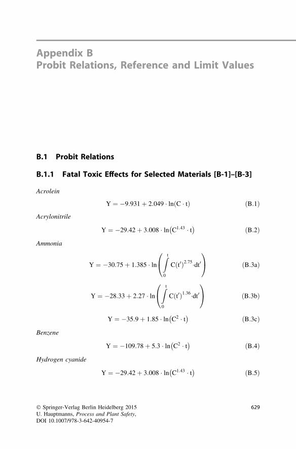
B.1.1 Fatal Toxic Effects for Selected Materials [B-1]–[B-3]

Acrolein

Y ¼ �9:931þ 2:049 � ln C � tð Þ ðB:1Þ

Acrylonitrile

Y ¼ �29:42þ 3:008 � ln C1:43 � t� �

ðB:2Þ

Ammonia

Y ¼ �30:75þ 1:385 � lnZ t

0

C t0ð Þ2:75�dt0

0

@

1

A ðB:3aÞ

Y ¼ �28:33þ 2:27 � lnZ t

0

C t0ð Þ1:36�dt0

0

@

1

A ðB:3bÞ

Y ¼ �35:9þ 1:85 � ln C2 � t� �

ðB:3cÞ

Benzene

Y ¼ �109:78þ 5:3 � ln C2 � t� �

ðB:4Þ

Hydrogen cyanide

Y ¼ �29:42þ 3:008 � ln C1:43 � t� �

ðB:5Þ


629

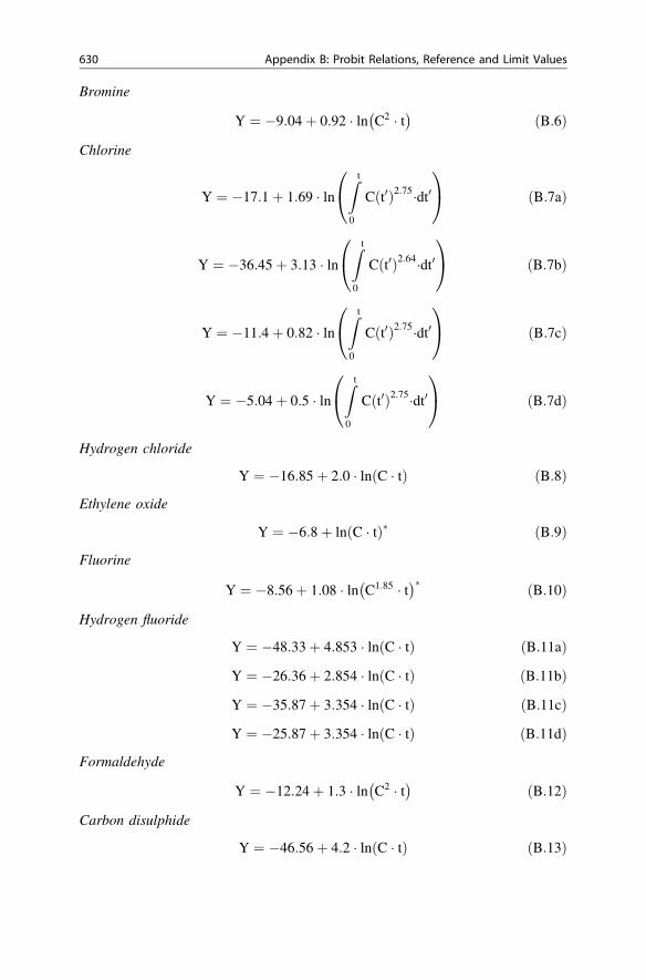
Bromine

Y ¼ �9:04þ 0:92 � ln C2 � t� �

ðB:6Þ

Chlorine

Y ¼ �17:1þ 1:69 � lnZ t

0

C t0ð Þ2:75�dt0

0

@

1

A ðB:7aÞ

Y ¼ �36:45þ 3:13 � lnZ t

0

C t0ð Þ2:64�dt0

0

@

1

A ðB:7bÞ

Y ¼ �11:4þ 0:82 � lnZ t

0

C t0ð Þ2:75�dt0

0

@

1

A ðB:7cÞ

Y ¼ �5:04þ 0:5 � lnZ t

0

C t0ð Þ2:75�dt0

0

@

1

A ðB:7dÞ

Hydrogen chloride

Y ¼ �16:85þ 2:0 � ln C � tð Þ ðB:8Þ

Ethylene oxide

Y ¼ �6:8þ ln C � tð Þ� ðB:9Þ

Fluorine

Y ¼ �8:56þ 1:08 � ln C1:85 � t� �� ðB:10Þ

Hydrogen fluoride

Y ¼ �48:33þ 4:853 � ln C � tð Þ ðB:11aÞ

Y ¼ �26:36þ 2:854 � ln C � tð Þ ðB:11bÞ

Y ¼ �35:87þ 3:354 � ln C � tð Þ ðB:11cÞ

Y ¼ �25:87þ 3:354 � ln C � tð Þ ðB:11dÞ

Formaldehyde

Y ¼ �12:24þ 1:3 � ln C2 � t� �

ðB:12Þ

Carbon disulphide

Y ¼ �46:56þ 4:2 � ln C � tð Þ ðB:13Þ

630 Appendix B: Probit Relations, Reference and Limit Values

Carbon monoxide

Y ¼ �37:98þ 3:7 � ln C � tð Þ ðB:14Þ

Methanol

Y ¼ �6:34734þ 0:66358 � ln C � tð Þ ðB:15Þ

Fuming sulphuric acid (oleum)

Y ¼ �14:2þ 1:6 � ln C1:8 � t� �� ðB:16Þ

Phosgene

Y ¼ �27:2þ 5:1 � ln C � tð Þ ðB:17aÞ

Y ¼ �19:27þ 3:686 � ln C � tð Þ ðB:17bÞ

Phosphine

Y ¼ �2:25þ ln C � tð Þ ðB:18Þ

Sulphur dioxide

Y ¼ �15:67þ 2:1 � ln C � tð Þ ðB:19Þ

Hydrogen sulphide

Y ¼ �11:15þ ln C1:9 � t� �

ðB:20Þ

Toluene

Y ¼ �6:794þ 0:408 � ln C2:5 � t� �

ðB:21Þ

where C(t) is the time-dependent concentration in ppm and the time is in minutes(exception: * in mg/m3 and minutes).

B.1.2 Pressure and Heat Radiation Exposures [B-1, B-4]

Death from lung haemorrhage due to a blast wave

Y ¼ �77:1þ 6:91 � ln ps ðB:22Þ

Eardrum rupture due to a blast wave

Y ¼ �15:6þ 1:93 � ln ps ðB:23aÞ

Y ¼ �12:6þ 1:524 � ln ps ðB:23bÞ

Death following body translation due to impulse

Y ¼ �46:1þ 4:82 � ln J ðB:24Þ

Appendix B: Probit Relations, Reference and Limit Values 631

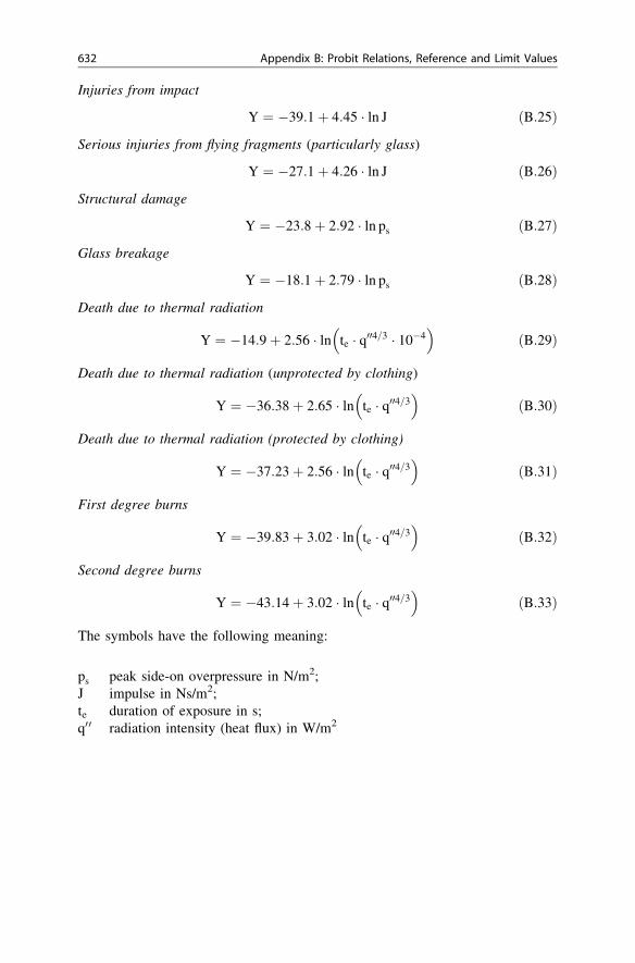
Injuries from impact

Y ¼ �39:1þ 4:45 � ln J ðB:25Þ

Serious injuries from flying fragments (particularly glass)

Y ¼ �27:1þ 4:26 � ln J ðB:26Þ

Structural damage

Y ¼ �23:8þ 2:92 � ln ps ðB:27Þ

Glass breakage

Y ¼ �18:1þ 2:79 � ln ps ðB:28Þ

Death due to thermal radiation

Y ¼ �14:9þ 2:56 � ln te � q004=3 � 10�4� �

ðB:29Þ

Death due to thermal radiation (unprotected by clothing)

Y ¼ �36:38þ 2:65 � ln te � q004=3� �

ðB:30Þ

Death due to thermal radiation (protected by clothing)

Y ¼ �37:23þ 2:56 � ln te � q004=3� �

ðB:31Þ

First degree burns

Y ¼ �39:83þ 3:02 � ln te � q004=3� �

ðB:32Þ

Second degree burns

Y ¼ �43:14þ 3:02 � ln te � q004=3� �

ðB:33Þ

The symbols have the following meaning:

ps peak side-on overpressure in N/m2;J impulse in Ns/m2;te duration of exposure in s;q00 radiation intensity (heat flux) in W/m2


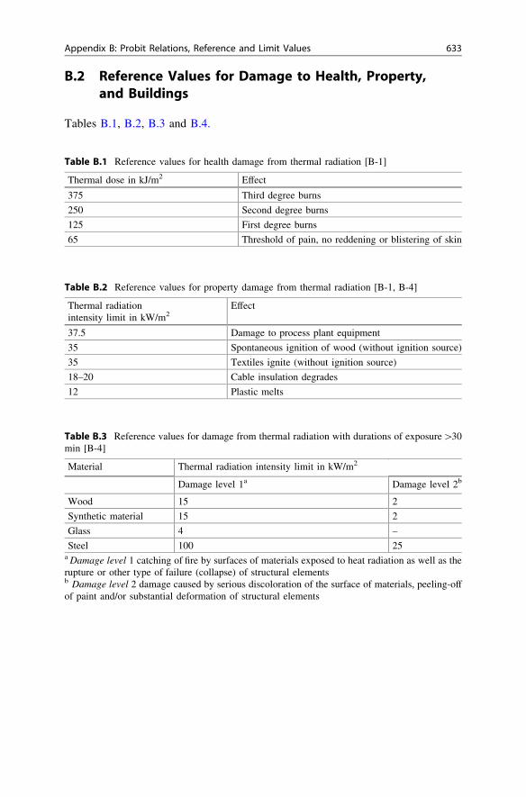
B.2 Reference Values for Damage to Health, Property,and Buildings

Tables B.1, B.2, B.3 and B.4.


Table B.1 Reference values for health damage from thermal radiation [B-1]

Thermal dose in kJ/m2 Effect

375 Third degree burns

250 Second degree burns

125 First degree burns

65 Threshold of pain, no reddening or blistering of skin

Table B.2 Reference values for property damage from thermal radiation [B-1, B-4]

Thermal radiationintensity limit in kW/m2

Effect

37.5 Damage to process plant equipment

35 Spontaneous ignition of wood (without ignition source)

35 Textiles ignite (without ignition source)

18–20 Cable insulation degrades

12 Plastic melts

Table B.3 Reference values for damage from thermal radiation with durations of exposure[30min [B-4]

Material Thermal radiation intensity limit in kW/m2

Damage level 1a Damage level 2b

Wood 15 2

Synthetic material 15 2

Glass 4 –

Steel 100 25a Damage level 1 catching of fire by surfaces of materials exposed to heat radiation as well as therupture or other type of failure (collapse) of structural elementsb Damage level 2 damage caused by serious discoloration of the surface of materials, peeling-offof paint and/or substantial deformation of structural elements

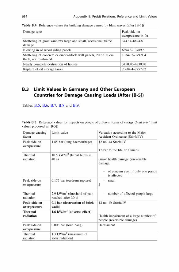
B.3 Limit Values in Germany and Other EuropeanCountries for Damage Causing Loads (After [B-5])

Tables B.5, B.6, B.7, B.8 and B.9.

Table B.4 Reference values for building damage caused by blast waves (after [B-1])

Damage type Peak side-onoverpressure in Pa

Shattering of glass windows large and small, occasional framedamage

3447.4–6894.8

Blowing in of wood siding panels 6894.8–13789.6

Shattering of concrete or cinder-block wall panels, 20 or 30 cmthick, not reinforced

10342.2–37921.4

Nearly complete destruction of houses 34500.0–48300.0

Rupture of oil storage tanks 20684.4–27579.2

Table B.5 Reference values for impacts on people of different forms of energy (bold print limitvalues proposed in [B-5])

Damage causingfactor

Limit value Valuation according to the MajorAccident Ordinance (StörfallV)

Peak side-onoverpressure

1.85 bar (lung haemorrhage) §2 no. 4a StörfallV

Threat to the life of humans

Thermalradiation

10.5 kW/m2 (lethal burns in40 s) Grave health damage (irreversible

damage)

- of concern even if only one personis affected


0.175 bar (eardrum rupture) - small;

Thermalradiation

2.9 kW/m2 (threshold of painreached after 30 s)

- number of affected people large


0.1 bar (destruction of brickwalls)

§2 no. 4b StörfallV

Thermalradiation

1.6 kW/m2 (adverse effect)Health impairment of a large number ofpeople (reversible damage)


0.003 bar (loud bang) Harassment

Thermalradiation

1.3 kW/m2 (maximum ofsolar radiation)


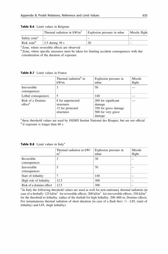
Table B.6 Limit values in Belgium

Thermal radiation in kW/m2 Explosion pressure in mbar Missile flight

Safety zonea – – –

Risk zoneb 2.5 during 30 s 20 –a Zone, where reversible effects are observedb Zone, where specific measures must be taken for limiting accident consequences with dueconsideration of the duration of exposure

Table B.7 Limit values in France

Thermal radiationb inkW/m

Explosion pressure inmbar

Missileflight

Irreversibleconsequences

3 50 —

Lethal consequences 5 140 —

Risk of a Dominoeffecta

8 for unprotectedstructures12 for protectedstructures

200 for significantdamage350 for grave damage500 for very gravedamage

—

a these threshold values are used by INERIS Institut National des Risques, but are not officialb if exposure is longer than 60 s


Table B.8 Limit values in Italya

Thermal radiation in kW/m2


Missileflight

Reversibleconsequences

3 30 –

Irreversibleconsequences

5 70 –

Start of lethality 7 140 –

High risk of lethality 12.5 300 –

Risk of a domino effect 12.5 300 –a In Italy the following threshold values are used as well for non-stationary thermal radiation (incase of a fireball): 125 kJ/m2 for reversible effects, 200 kJ/m2 for irreversible effects, 350 kJ/m2

for the threshold to lethality, radius of the fireball for high lethality: 200–800 m, Domino effects.For instantaneous thermal radiation of short duration (in case of a flash fire): � � LFL (start oflethality) and LFL (high lethality)

References

[B-1] Mannan S (ed) (2005) Lees’ loss prevention in the process industries, hazard identification,assessment and control, 3rd edn. Elsevier, Amsterdam

[B-2] Louvar JF, Louvar BD (1998) Health and environmental risk analysis: fundamentals withapplications, vol 2. Prentice Hall, Upper Saddle River

[B-3] PHAST Version 6.51 (2006)

[B-4] The Director-General of Labour (1989) Methods for the determination of possible damageto people and objects resulting from the release of hazardous materials. Green Book,Voorburg, December 1989

[B-5] Kommission für Anlagensicherheit beim Bundesminister für Umwelt, Naturschutz undReaktorsicherheit, Leitfaden ,,Empfehlung für Abstände zwischen Betriebsbereichen nachder Störfall-Verordnung und schutzbedürftigen Gebieten im Rahmen der Bauleitplanung-Umsetzung §50 BImSchG, 2. Überarbeitete Fassung, KAS-18, November 2010Short version of Guidance KAS-18 (2014) Recommendations for separation distancesbetween establishments covered by the major accidents ordinance (Störfall-Verordnung)and areas worthy of protection within the framework of land-use planning implementationof Article 50 of the Federal Immission Control Act (Bundes-Immissionsschutzgesetz,BImSchG). http://www.kas-u.de/publikationen/pub_gb.htm. Last visited on 13 May 2014

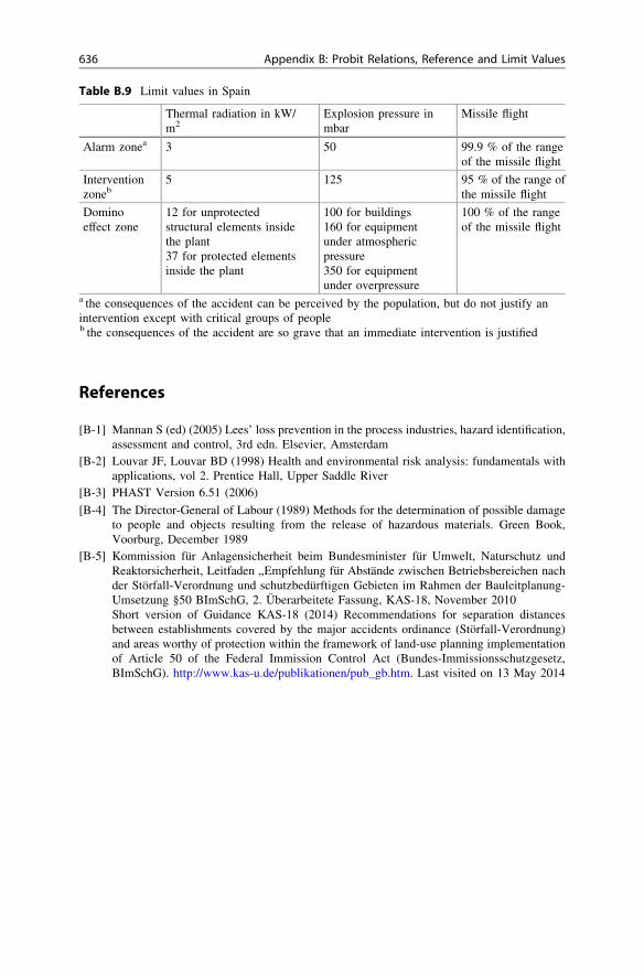
Table B.9 Limit values in Spain

Thermal radiation in kW/m2


Missile flight

Alarm zonea 3 50 99.9 % of the rangeof the missile flight

Interventionzoneb

5 125 95 % of the range ofthe missile flight

Dominoeffect zone

12 for unprotectedstructural elements insidethe plant37 for protected elementsinside the plant

100 for buildings160 for equipmentunder atmosphericpressure350 for equipmentunder overpressure

100 % of the rangeof the missile flight

a the consequences of the accident can be perceived by the population, but do not justify anintervention except with critical groups of peopleb the consequences of the accident are so grave that an immediate intervention is justified


http://www.kas-u.de/publikationen/pub_gb.htm

Appendix CBasics of Probability Calculations

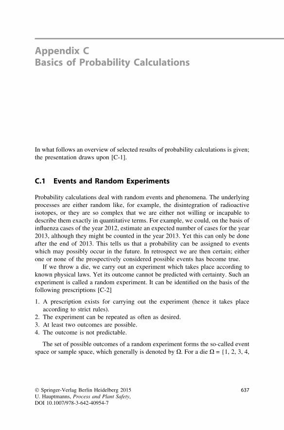
In what follows an overview of selected results of probability calculations is given;the presentation draws upon [C-1].

C.1 Events and Random Experiments

Probability calculations deal with random events and phenomena. The underlyingprocesses are either random like, for example, the disintegration of radioactiveisotopes, or they are so complex that we are either not willing or incapable todescribe them exactly in quantitative terms. For example, we could, on the basis ofinfluenza cases of the year 2012, estimate an expected number of cases for the year2013, although they might be counted in the year 2013. Yet this can only be doneafter the end of 2013. This tells us that a probability can be assigned to eventswhich may possibly occur in the future. In retrospect we are then certain; eitherone or none of the prospectively considered possible events has become true.

If we throw a die, we carry out an experiment which takes place according toknown physical laws. Yet its outcome cannot be predicted with certainty. Such anexperiment is called a random experiment. It can be identified on the basis of thefollowing prescriptions [C-2]

1. A prescription exists for carrying out the experiment (hence it takes placeaccording to strict rules).

2. The experiment can be repeated as often as desired.3. At least two outcomes are possible.4. The outcome is not predictable.

The set of possible outcomes of a random experiment forms the so-called eventspace or sample space, which generally is denoted by X. For a die X = {1, 2, 3, 4,


637

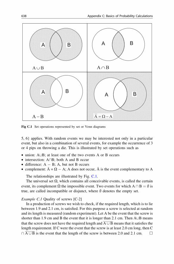
5, 6} applies. With random events we may be interested not only in a particularevent, but also in a combination of several events, for example the occurrence of 3or 4 pips on throwing a die. This is illustrated by set operations such as

• union: A[B; at least one of the two events A or B occurs• intersection: A\B; both A and B occur• difference: A - B; A, but not B occurs• complement: A = X - A; A does not occur, A is the event complementary to A

The relationships are illustrated by Fig. C.1.The universal set X, which contains all conceivable events, is called the certain

event, its complement �X the impossible event. Two events for which A \ B ¼ ; istrue, are called incompatible or disjunct, where ; denotes the empty set.

Example C.1 Quality of screws [C-2]In a production of screws we wish to check, if the required length, which is to lie

between 1.9 and 2.1 cm, is satisfied. For this purpose a screw is selected at randomand its length is measured (random experiment). Let A be the event that the screw isshorter than 1.9 cm and B the event that it is longer than 2.1 cm. Then A[B meansthat the screw does not have the required length and A [ B means that it satisfies thelength requirement. If C were the event that the screw is at least 2.0 cm long, then C\ A [ B is the event that the length of the screw is between 2.0 and 2.1 cm. h

638 Appendix C: Basics of Probability Calculations

Fig C.1 Set operations represented by set or Venn diagrams

C.2 Probabilities

One cannot predict the outcome of a random experiment, but it is possible toindicate a probability for a particular outcome. Thus it is known that 5 pips showup with a probability of 1/6 when throwing an ideal die. If this event is denoted byC we write

P Cð Þ ¼ 16

ðC:1Þ

Since it is mathematically inexact to base areas of knowledge on experimentswith ideal—but in reality non-existent—objects, Kolmogoroff established axioms.These axioms, however, comprise the results which would intuitively be expectedif the experiment were repeated an infinite number of times. The axioms are

1.

P Að Þ� 0 for any event A � X ðpositivityÞ

2.

P Xð Þ ¼ 1 ðunitarityÞ ðC:2Þ

3.

P[1

i¼1

Ai

!

¼X1

i¼1

P Aið Þ ðr� additivityÞ

The third property of course implies the finite additivity

P[n

i¼1

Ai

!

¼Xn

i¼1

P Aið Þ ðC:3Þ

If there are just two disjunct (mutually exclusive) events, A and B, we have

P A [ Bð Þ ¼ P Að Þ þ P Bð Þ ðC:4Þ

All calculation rules for probabilities can be derived from the above properties,e.g.

P A [ Bð Þ ¼ P Að Þ þ P Bð Þ � P A \ Bð Þ for any arbitrary A and B

P �Að Þ ¼ 1� P Að Þ ðC:5Þ

P A� Bð Þ ¼ P Að Þ � P Bð Þ; if B � A

Appendix C: Basics of Probability Calculations 639

Example C.2 Game of DiceWe are looking for the probability that when throwing a die two or four pips

appear. This event is described by the set {2, 4}. According to Eq. (C.4) we have

P 2; 4f gð Þ ¼ P 2f gð Þ þ P 4f gð Þ

¼ 16þ 1

6¼ 1

3

Another way of solving the problem consists in subtracting from the certain eventall events which we are not looking for, i.e.

P 2; 4f gð Þ ¼ P 1; 2; 3; 4; 5; 6f gð Þ � P 1; 3; 5; 6f gð Þ¼ 1� P 1f gð Þ � P 3f gð Þ � P 5f gð Þ � P 6f gð Þ

¼ 1� 16� 1

6� 1

6� 1

6¼ 1

3:

h

C.3 Conditional Probabilities and Independence

Often we are interested in the probability of the occurrence of an event A under thecondition that a particular event B has already occurred. For example, the failureof a pump in a process plant under the condition that the plant has been flooded.Such a probability is called conditional probability. It is explained below usingexamples from [C-2].

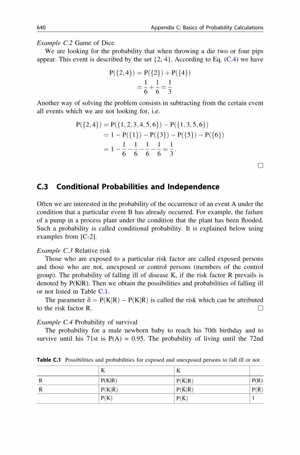
Example C.3 Relative riskThose who are exposed to a particular risk factor are called exposed persons

and those who are not, unexposed or control persons (members of the controlgroup). The probability of falling ill of disease K, if the risk factor R prevails isdenoted by P(K|R). Then we obtain the possibilities and probabilities of falling illor not listed in Table C.1.

The parameter d ¼ P K Rjð Þ � P K �Rjð Þ is called the risk which can be attributedto the risk factor R. h

Example C.4 Probability of survivalThe probability for a male newborn baby to reach his 70th birthday and to

survive until his 71st is P(A) = 0.95. The probability of living until the 72nd


Table C.1 Possibilities and probabilities for exposed and unexposed persons to fall ill or not

K �K

R P(K|R) P �KjRð Þ P(R)�R P Kj�Rð Þ P �Kj�Rð Þ P �Rð Þ

P Kð Þ P �Kð Þ 1

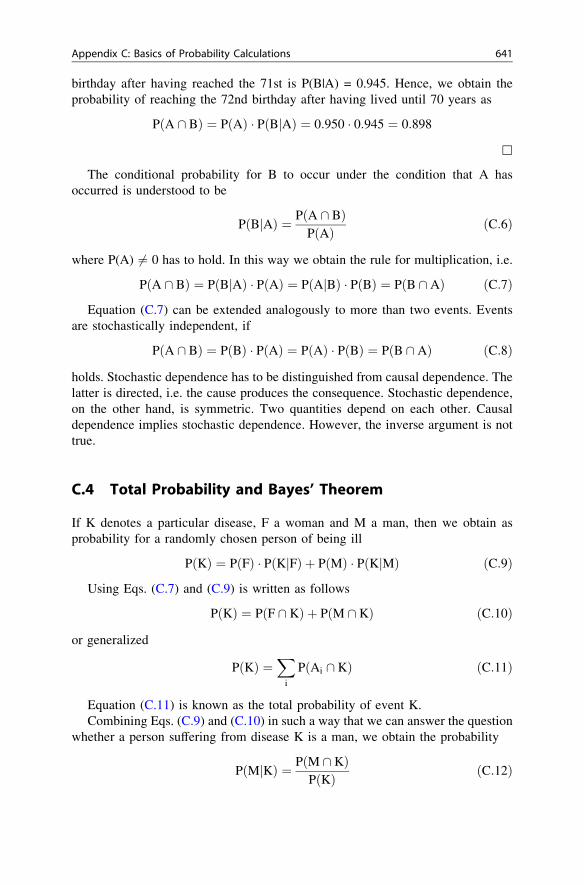
birthday after having reached the 71st is P(B|A) = 0.945. Hence, we obtain theprobability of reaching the 72nd birthday after having lived until 70 years as

P A \ Bð Þ ¼ P Að Þ � P B Ajð Þ ¼ 0:950 � 0:945 ¼ 0:898

h

The conditional probability for B to occur under the condition that A hasoccurred is understood to be

P B Ajð Þ ¼ P A \ Bð ÞP Að Þ ðC:6Þ

where P(A) 6¼ 0 has to hold. In this way we obtain the rule for multiplication, i.e.

P A \ Bð Þ ¼ P B Ajð Þ � P Að Þ ¼ P A Bjð Þ � P Bð Þ ¼ P B \ Að Þ ðC:7Þ

Equation (C.7) can be extended analogously to more than two events. Eventsare stochastically independent, if

P A \ Bð Þ ¼ P Bð Þ � P Að Þ ¼ P Að Þ � P Bð Þ ¼ P B \ Að Þ ðC:8Þ

holds. Stochastic dependence has to be distinguished from causal dependence. Thelatter is directed, i.e. the cause produces the consequence. Stochastic dependence,on the other hand, is symmetric. Two quantities depend on each other. Causaldependence implies stochastic dependence. However, the inverse argument is nottrue.

C.4 Total Probability and Bayes’ Theorem

If K denotes a particular disease, F a woman and M a man, then we obtain asprobability for a randomly chosen person of being ill

P Kð Þ ¼ P Fð Þ � P K Fjð Þ þ P Mð Þ � P K Mjð Þ ðC:9Þ

Using Eqs. (C.7) and (C.9) is written as follows

P Kð Þ ¼ P F \ Kð Þ þ P M \ Kð Þ ðC:10Þ

or generalized

P Kð Þ ¼X

i

P Ai \ Kð Þ ðC:11Þ

Equation (C.11) is known as the total probability of event K.Combining Eqs. (C.9) and (C.10) in such a way that we can answer the question

whether a person suffering from disease K is a man, we obtain the probability

P M Kjð Þ ¼ P M \ Kð ÞP Kð Þ ðC:12Þ


In Eq. (C.12) we ask for a particular circumstance related to an event. In thepresent context the question is if a person affected by the disease K (event) is aman (circumstance).

Inserting Eq. (C.10) in Eq. (C.12) and using Eq. (C.9), one obtains

P M Kjð Þ ¼ P K Mjð Þ � P Mð ÞP Fð Þ � P K Fjð Þ þ P Mð Þ � P K Mjð Þ ðC:13Þ

In this way we obtain Bayes’ theorem, which in generalized form reads

P Ak Kjð Þ ¼ P Akð Þ � P K Akjð ÞPn

i¼1 P Aið Þ � P K Aijð Þ ðC:14Þ

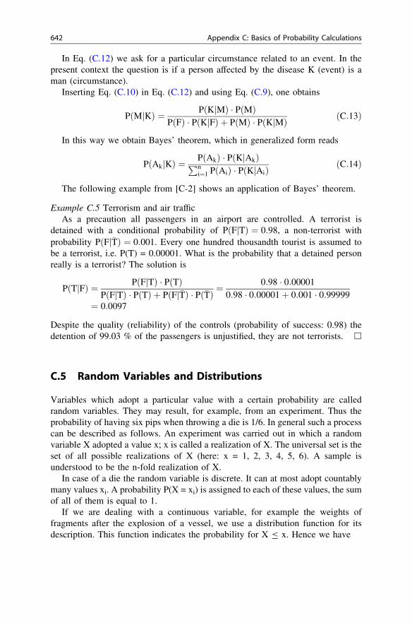
The following example from [C-2] shows an application of Bayes’ theorem.

Example C.5 Terrorism and air trafficAs a precaution all passengers in an airport are controlled. A terrorist is

detained with a conditional probability of P F Tjð Þ ¼ 0:98, a non-terrorist withprobability P F �Tjð Þ ¼ 0:001. Every one hundred thousandth tourist is assumed tobe a terrorist, i.e. P(T) = 0.00001. What is the probability that a detained personreally is a terrorist? The solution is

P T Fjð Þ ¼ P F Tjð Þ � P Tð ÞP F Tjð Þ � P Tð Þ þ P F �Tjð Þ � P �Tð Þ ¼

0:98 � 0:000010:98 � 0:00001þ 0:001 � 0:99999

¼ 0:0097

Despite the quality (reliability) of the controls (probability of success: 0.98) thedetention of 99.03 % of the passengers is unjustified, they are not terrorists. h

C.5 Random Variables and Distributions

Variables which adopt a particular value with a certain probability are calledrandom variables. They may result, for example, from an experiment. Thus theprobability of having six pips when throwing a die is 1/6. In general such a processcan be described as follows. An experiment was carried out in which a randomvariable X adopted a value x; x is called a realization of X. The universal set is theset of all possible realizations of X (here: x = 1, 2, 3, 4, 5, 6). A sample isunderstood to be the n-fold realization of X.

In case of a die the random variable is discrete. It can at most adopt countablymany values xi. A probability P(X = xi) is assigned to each of these values, the sumof all of them is equal to 1.

If we are dealing with a continuous variable, for example the weights offragments after the explosion of a vessel, we use a distribution function for itsdescription. This function indicates the probability for X B x. Hence we have


F xð Þ ¼ P X� xð Þ ðC:15Þ

F(x) is thus defined for all real numbers. F(x) is also called the cumulativedistribution function. If F(x) is differentiable, which normally is the case, weobtain its probability density function (pdf)

f tð Þ ¼ P t�X� tþ dtð Þ ðC:16Þ

Equation (C.16) is the probability for X lying between t and t + dt.By combining Eqs. (C.15) and (C.16) we obtain

F xð Þ ¼Zx

�1

f tð Þdt withZ1

�1

f tð Þdt ¼ 1 ðC:17Þ

Probability distributions are characterised by so-called moments. The firstmoment is the expected value. In case of discrete variables we have

EðXÞ ¼Xn

i¼1

xi � P X ¼ xið Þ ðC:18Þ

and for continuous variables

EðXÞ ¼Z1

�1

t � f tð Þdt ðC:19Þ

Furthermore the variance is used. It is obtained from

V Xð Þ ¼ E X� E Xð Þð Þ2h i

ðC:20Þ

Using Steiner’s theorem Eq. (C.20) becomes

V Xð Þ ¼ E X2� �

� E Xð Þ2 ðC:21Þ

where E X2� �

is the second moment. The square root of the variance is calledstandard deviation, i.e.

S Xð Þ ¼ffiffiffiffiffiffiffiffiffiffiffiV Xð Þ

pðC:22Þ

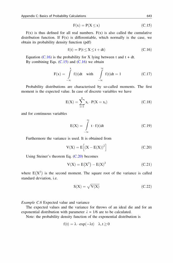
Example C.6 Expected value and varianceThe expected values and the variance for throws of an ideal die and for an

exponential distribution with parameter k = 1/6 are to be calculated.Note: the probability density function of the exponential distribution is

f tð Þ ¼ k � exp �ktð Þ k; t� 0


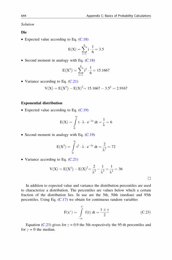
Solution

Die

• Expected value according to Eq. (C.18)

E Xð Þ ¼X6

i¼1

i � 16¼ 3:5

• Second moment in analogy with Eq. (C.18)

E X2� �

¼X6

i¼1

i2 � 16¼ 15:1667

• Variance according to Eq. (C.21)

V Xð Þ ¼ E X2� �

� E Xð Þ2¼ 15:1667� 3:52 ¼ 2:9167

Exponential distribution

• Expected value according to Eq. (C.19)

EðXÞ ¼Z1

0

t � k � e�kt dt ¼ 1k¼ 6

• Second moment in analogy with Eq. (C.19)

EðX2Þ ¼Z1

0

t2 � k � e�kt dt ¼ 2

k2 ¼ 72

• Variance according to Eq. (C.21)

V Xð Þ ¼ E X2� �

� E Xð Þ2¼ 2

k2 �1

k2 ¼1

k2 ¼ 36

h

In addition to expected value and variance the distribution percentiles are usedto characterize a distribution. The percentiles are values below which a certainfraction of the distribution lies. In use are the 5th, 50th (median) and 95thpercentiles. Using Eq. (C.17) we obtain for continuous random variables

F x�ð Þ ¼Zx�

�1

f tð Þ dt ¼ 1� c2

ðC:23Þ

Equation (C.23) gives for c = 0.9 the 5th respectively the 95-th percentiles andfor c = 0 the median.


C.6 Selected Types of Distributions

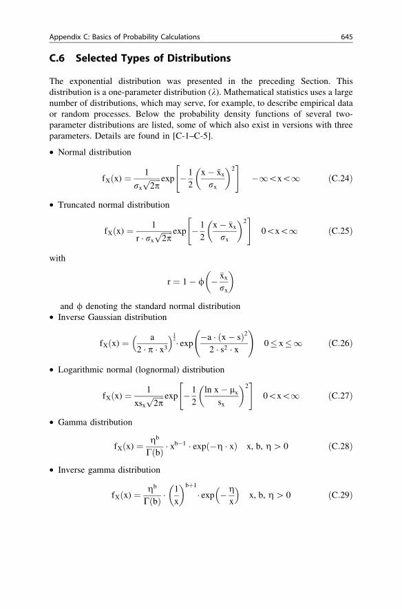
The exponential distribution was presented in the preceding Section. Thisdistribution is a one-parameter distribution (k). Mathematical statistics uses a largenumber of distributions, which may serve, for example, to describe empirical dataor random processes. Below the probability density functions of several two-parameter distributions are listed, some of which also exist in versions with threeparameters. Details are found in [C-1–C-5].

• Normal distribution

fXðx) ¼ 1

rx

ffiffiffiffiffiffi2pp exp � 1

2x� �xx

rx

� �2" #

�1\x\1 ðC:24Þ

• Truncated normal distribution

fXðx) ¼ 1

r � rx


2x� �xx

rx

� �2" #

0\x\1 ðC:25Þ

with

r ¼ 1� / � �xx

rx

� �

and / denoting the standard normal distribution• Inverse Gaussian distribution

fXðx) ¼ a2 � p � x3

� �12� exp

�a � x� sð Þ2

2 � s2 � x

!

0� x�1 ðC:26Þ

• Logarithmic normal (lognormal) distribution

fXðx) ¼ 1

xsx


2ln x� lx

sx

� �2" #

0\x\1 ðC:27Þ

• Gamma distribution

fXðx) ¼ gb

C bð Þ � xb�1 � exp �g � xð Þ x, b, g [ 0 ðC:28Þ

• Inverse gamma distribution

fXðx) ¼ gb

C bð Þ �1x

� �bþ1

� exp �gx

� �x, b, g [ 0 ðC:29Þ


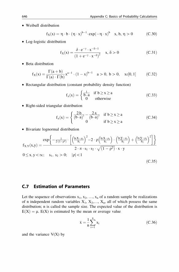
• Weibull distribution

fXðx) ¼ g � b � g � xð Þb�1� exp �g � xð Þb x, b, g [ 0 ðC:30Þ

• Log-logistic distribution

fXðx) ¼ d � e�c � x�d�1

1þ e�c � x�dð Þ2x, d[ 0 ðC:31Þ

• Beta distribution

fXðx) ¼ C aþ bð ÞC að Þ � C bð Þ x

a�1 � 1� xð Þb�1 a [ 0; b [ 0; xe 0; 1½ ðC:32Þ

• Rectangular distribution (constant probability density function)

fxðxÞ ¼1

b�a if b� x� a

0 otherwise

ðC:33Þ

• Right-sided triangular distribution

fxðxÞ ¼2�b

b�að Þ2 �2�x

b�að Þ2 if b� x� a

0 if b� x� a

(

ðC:34Þ

• Bivariate lognormal distribution

fX;Y x,yð Þ ¼exp � 1

2� 1�q2ð Þ �ln x�l1

s1

� �2�2 � q ln x�l1

s1

� �� ln y�l2

s2

� �þ ln y�l2

s2

� �2 � �

2 � p � s1 � s2 �ffiffiffiffiffiffiffiffiffiffiffiffiffiffiffiffiffi1� q2ð Þ

p� x � y

0� x; y\1; s1; s2 [ 0; qj j\1

ðC:35Þ

C.7 Estimation of Parameters

Let the sequence of observations x1, x2, …, xn of a random sample be realizationsof n independent random variables X1, X2,…, Xn, all of which possess the samedistribution; n is called the sample size. The expected value of the distribution isEðXÞ ¼ l. E(X) is estimated by the mean or average value

�x ¼ 1n

Xn

i¼1

xi ðC:36Þ

and the variance V(X) by


r2 ¼ 1n� 1

Xn

1¼1

x2i � n�x2

!

ðC:37Þ

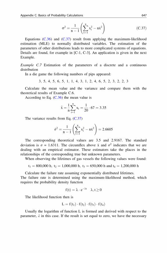
Equations (C.36) and (C.37) result from applying the maximum-likelihoodestimation (MLE) to normally distributed variables. The estimation of theparameters of other distributions leads to more complicated systems of equations.Details are found, for example in [C-1, C-3]. An application is given in the nextExample.

Example C.7 Estimation of the parameters of a discrete and a continuousdistribution

In a die game the following numbers of pips appeared:

3; 5; 4; 5; 6; 5; 1; 1; 4; 3; 1; 2; 4; 6; 5; 2; 3; 2; 2; 3

Calculate the mean value and the variance and compare them with thetheoretical results of Example C.6.

According to Eq. (C.36) the mean value is

�x ¼ 1n

Xn

i¼1

xi ¼1

20� 67 ¼ 3:35

The variance results from Eq. (C.37)

r2 ¼ 1n� 1

Xn

1¼1

x2i � n�x2

!

¼ 2:6605

The corresponding theoretical values are 3.5 and 2.9167. The standarddeviation is r = 1.6311. The circumflex above �x and r2 indicates that we aredealing with an empirical estimator. These estimators take the places in therelationships of the corresponding true but unknown parameters.

When observing the lifetimes of gas vessels the following values were found:

t1 ¼ 800,000 h; t2 ¼ 1,000,000 h; t3 ¼ 650,000 h and t4 ¼ 1,200,000 h

Calculate the failure rate assuming exponentially distributed lifetimes.The failure rate is determined using the maximum-likelihood method, whichrequires the probability density function

f tð Þ ¼ k � e�kt k; t� 0

The likelihood function then is

L ¼ f t1ð Þ � f t2ð Þ � f t3ð Þ � f t4ð Þ

Usually the logarithm of function L is formed and derived with respect to theparameter, k in this case. If the result is set equal to zero, we have the necessary


condition for the maximum of the function, from which k is determined.

d ln Ldk¼ 4

k� t1 þ t2 þ t3 þ t4ð Þ

where from

k ¼ 4t1 þ t2 þ t3 þ t4

¼ 1:1 � 10�6 h�1

results. h

C.8 Probability Trees

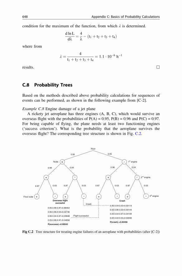
Based on the methods described above probability calculations for sequences ofevents can be performed, as shown in the following example from [C-2].

Example C.8 Engine damage of a jet planeA rickety jet aeroplane has three engines (A, B, C), which would survive an

overseas flight with the probabilities of P(A) = 0.95, P(B) = 0.96 and P(C) = 0.97.For being capable of flying, the plane needs at least two functioning engines(‘success criterion’). What is the probability that the aeroplane survives theoverseas flight? The corresponding tree structure is shown in Fig. C.2.

+

+

+ -

-

+ -

Root

0.95

0.96

0.97

0.04

0.030,970.03

0.05

-

+

+ -

-

+ -

0.970.030.97 0.03

0.96 0.04

Node

Final node

1st engine

2nd engine

3rd engine

Overseas flight succesful

0.95·0.96·0.97=0.88464

0.95·0.96·0.03=0.02736

0.95·0.04·0.97=0.03648

0.05·0.96·0.97=0.04656

P(success) =0.99542

Crash

0.95·0.04·0.03=0.00114

0.05·0.96·0.03=0.00144

0.05·0.04·0.97=0.00194

0.05·0.04·0.03=0.00006

P(crash) =0.00458

Flight successful

Crash

Fig C.2 Tree structure for treating engine failures of an aeroplane with probabilities (after [C-2])


The flight is successful if any one of the following situations occurs:

• engines A and B survive, C fails

PðA \ B \ CÞ ¼ P Að Þ � P Bð Þ � 1� P Cð Þð Þ ¼ 0:02736

• engines B and C survive, A fails

PðB \ C \ AÞ ¼ P Bð Þ � P Cð Þ � 1� P Að Þð Þ ¼ 0:04656

• engines A and C survive, B fails

PðA \ C \ BÞ ¼ P Að Þ � P Cð Þ � 1� P Bð Þð Þ ¼ 0:03686

• all engines survive

PðA \ C \ BÞ ¼ P Að Þ � P Bð Þ � P Cð Þ ¼ 0:88464

Since we are dealing with mutually exclusive events the total probability of asuccessful flight is calculated according to Eq. (C.4), which gives

P successful flightð Þ ¼ 0:99542 and hence P crashð Þ ¼ 0:00458:

h

References

[C-1] Hartung J (1991) Statistik: Lehr- und Handbuch der angewandten Statistik. R. OldenbourgVerlag, München

[C-2] Sachs L (1999) Angewandte Statistik—Anwendung statistischer Methoden. Springer,Heidelberg

[C-3] Härtler G (1983) Statistische Modelle für die Zuverlässigkeitsanalyse. VEB VerlagTechnik, Berlin

[C-4] Abramowitz M, Stegun IA (eds) (1972) Handbook of mathematical functions withformulas, graphs, and mathematical tables. Department of Commerce, Washington

[C-5] Johnson NL, Kotz S, Balakrishnan N (1995) Continuous univariate distributions, vol 2.Wiley, New York


Appendix DCoefficients for the TNO Multienergy Modeland the BST Model

Tables D.1 and D.2.


651

652 Appendix D: Coefficients for the TNO Multienergy Model and the BST Model

Table D.1 Coefficients for the TNO multienergy model Eq. (10.163) [D-1–D-3]

Explosion strength Range a b c d

Curve 1 0.23 B x B 0.53 1.00�10-2

x [ 0.53 6.23�10-3 -0.95

Curve 2 0.23 B x B 0.60 1.00�10-2

x [ 0.60 1.22�10-2 -0.98

Curve 3 0.23 B x B 0.60 5.00�10-2

x [ 0.60 3.05�10-2 -0.97

Curve 4 0.23 B x B 0.55 1.00�10-1

x [ 0.55 6.20�10-2 -0.97

Curve 5 0.23 B x B 0.55 2.00�10-1

x [ 0.55 1.10�10-1 -0.99

Curve 6 0.23 B x B 0.56 5.00�10-1

0.56 \ x B 3.50 3.00�10-1 -1.10

x [ 3.50 1.1188 0.5120

Curve 7 0.23 B x B 0.50 1.00�10-0

0.50 \ x B 1.00 4.60�10-1 -1.20

1.00 \ x B 2.50 1.5236 0.3372

x [ 2.50 1.1188 0.5120

Curve 8 0.23 B x B 0.50 2.00�10-0

0.50 \ x B 0.60 4.67�10-1 -2.08

0.60 \ x B 1.0 2.3721 0.3372

1.00 \ x B 2.50 1.5236 0.3372

x [ 2.50 1.1188 0.5120

Curve 9 0.23 B x B 0.35 5.00�10-0

0.35 \ x B 1.00 2.3721 0.3372

1.00 \ x B 2.50 1.5236 0.3372

x [ 2.50 1.1188 0.5120

Curve 10 0.23 B x B 1.00 2.3721 0.3372

1.00 \ x B 2.50 1.5236 0.3372

x [ 2.50 1.1188 0.5120

http://dx.doi.org/10.1007/978-3-642-40954-7_10

Ta

ble

D.2

Con

stan

tsfo

rth

eB

ST

mod

elE

q.(1

0.16

9)[D

-1,

D-4

]

Mf

xra

nge

ab

cd

ef

gh

pq

0.07

xB

0.15

0.15

\x

B2.

10x[

2.10

0.01 - -

-

-0.

9331

28-

-

-2.

8888

32-

-

-1.

7378

95-

-

0.92

0042

-

-

0.08

7748

-

-

-1.

0056

85-

-

-2.

3776

46-

- -

-1.

0117

36

- -

-2.

3656

16

0.12

xB

0.15

0.15

\x

B2.

10x[

2.10

0.02

8- -

-

-0.

9331

28-

-

-2.

8888

32-

-

-1.

7378

95-

-

0.92

0042

-

-

0.08

7748

-

-

-1.

0056

85-

-

-1.

9304

88-

- -

-1.

0117

36

- -

-1.

9184

58

0.20

xB

0.15

0.15

\x

B2.

10x[

2.10

0.06

5739

- -

-

-0.

9331

28-

-

-2.

8888

32-

-

-1.

7378

95-

-

0.92

0042

-

-

0.08

7748

-

-

-1.

0056

85-

-

-1.

5598

23-

- -

-1.

0117

36

- -

-1.

5477

93

0.35

xB

0.16

0.16

\x

B1.

70x[

1.70

0.21

8- -

-

-0.

0582

43-

-

-1.

5135

39-

-

-1.

5099

13-

-

0.60

2095

-

-

0.10

6104

-

-

-1.

0056

85-

-

-0.

9626

16-

- -

-0.

9965

87

- -

-1.

0379

88

0.70

xB

0.19

0.19

\x

B2.

37x[

2.37

0.68 - -

-

3.14

094

-

-

4.02

5197

-

-

-0.

5205

25-

-

-1.

6157

33-

-

-0.

5532

77-

-

-0.

7242

39-

-

-0.

5231

05-

- -

-1.

1601

57

- -

-0.

4941

53

1.00

xB

0.12

0.12

\x

B2.

26x[

2.26

1.24 - -

-

-2.

6507

31-

-

-5.

9756

78-

-

-2.

6554

64-

-

1.92

0581

-

-

0.41

7161

-

-

-1.

4083

33-

-

-0.

4887

46-

- -

-1.

1138

25

- -

-0.

5354

92

1.40

xB

0.17

0.17

\x

B2.

21x[

2.21

2.00 - -

-

-2.

3188

16-

-

-8.

1076

16-

-

-6.

8304

75-

-

1.07

0003

-

-

1.56

7781

-

-

-1.

3537

22-

-

-0.

4920

33-

- -

-1.

1389

89

- -

-0.

4755

84

2.00

xB

0.12

0.12

\x

B2.

27x[

2.27

5.00 - -

-

14.1

2624

-

-

22.5

5578

-

-

2.85

0864

-

-

-5.

8850

56-

-

-0.

1011

6-

-

-0.

9548

86-

-

-0.

4182

65-

- -

-1.

1745

14

- -

-0.

4154

06

3.00

xB

0.18

0.18

\x

B1.

86x[

1.86

10.0

0- -

-

-21

.675

65-

-

-11

.635

87-

-

7.95

783

-

-

1.56

914

-

-

-0.

5777

8-

-

-1.

2676

61-

-

-0.

3961

33-

- -

-1.

1745

14

- -

-0.

4154

06

4.00

xB

0.16

0.16

\x

B2.

25x[

2.25

15.2

- -

-

-14

.872

62-

-

-12

.509

94-

-

2.72

7597

-

-

1.73

1734

-

-

0.15

9062

-

-

-1.

3198

84-

-

-0.

4052

75-

- -

-1.

1745

14

- -

-0.

4154

06

5.20

xB

0.17

0.17

\x

B2.

27x[

2.27

20.0

- -

-

18.6

0017

5-

-

19.4

1657

1-

-

0.73

0754

-

-

-4.

4076

14-

-

-0.

0631

84-

-

-1.

0898

79-

-

-0.

3993

27-

- -

-1.

1745

14

- -

-0.

4154

06

Appendix D: Coefficients for the TNO Multienergy Model and the BST Model 653

http://dx.doi.org/10.1007/978-3-642-40954-7_10

References

[D-1] Arizal R (2012) Development of methodology for treating pressure waves from explosionsaccounting for modelling and data uncertainties. Dissertation, Fakultät für Verfahrens- undSystemtechnik, Otto-von-Guericke-Universität Magdeburg

[D-2] Alonso FD, Ferradas EG, Perez JFS, Aznar AM, Gimeno JR, Alonso JM (2006)Characteristic overpressure-impulse-distance curves for the detonation of explosives,pyrotechnics or unstable substances. J Loss Prev Process Ind 19:724–728

[D-3] Assael MJ, Kakosimos KE (2010) Fires, explosions, and toxic gas dispersions: effectcalculation and risk analysis. CRC Press Taylor & Francis Group, New York

[D-4] Det Norske Veritas (DNV) London, PHAST software version 6.7

654 Appendix D: Coefficients for the TNO Multienergy Model and the BST Model

Index

AAccident 1, 3–5, 7, 102, 118–119, 194–196,

269, 286, 323, 393, 603, 613, 615consequences, 220, 271, 273–275,

312–313, 441–586, 635–636definition, 2design basis, 6, 118scenarios, 270, 442–444, 584, 616

Activation, 117, 217, 218, 223, 286, 305–306,366, 381, 393, 402–403, 411–414, 417

Activation energy (apparent), 70, 76, 81, 85,130, 149

Actuarial approach, 270, 319, 578Aging, 290, 329, 331AGW value (workplace threshold), 58Air entrainment, 26

free jet, 473, 479dense gas dispersion, 503–504

Air resistance, 194, 470, 478, 561–564Airborne dispersion, 442, 489–501, 504, 505Alarm, 102, 103, 105, 114, 115, 118, 122, 210,

218, 219, 304–306, 308, 324–325,391, 392, 399, 402, 404–405, 407,411, 416–421, 602–606

Alarm and hazard defence plans, 101–102, 103ALARP (as low as reasonably practicable),

278, 279Aleatory uncertainty, 564ARIA (accident data bank), 8, 12Arrhenius, 70, 76, 81, 112, 123, 131–132,

223–224, 148, 214Atmospheric stability, 490, 491–492Autocatalytic reactions, 85–89Availability (cf. ‘‘unavailability’’), 100, 220,

293, 331, 356–378, 381definition, 287

BBaker-Strehlow-Tang Model (BST), 532,

544–550

Balance (safety), 284, 354Barrier, 103–104, 115, 220, 269, 273, 276,

309, 312–314, 320, 591, 594, 595,611

explosion, 231, 259–267Batch reactor, 71–73

semi-batch, 129–137Bathtub curve, 328–329Bayes, 7, 322–323, 339–343, 345, 445–448,

614, 641–642Beta Factor Model, 385–387, 411, 596–601Binary

(Boolean) variable, 311, 324, 345–352,394, 413

signal, 217Binomial distribution, 144, 336–337, 338–339,

340Biogas plant, 201–202Bow-tie diagram, 273Breather valve (pipe), 92, 255, 293Breathing, 92, 193, 198Breathing apparatus, 198, 201Brisance, 50, 533–534Brush discharge, 158, 159, 160, 168, 169, 175,

176BST model. See Baker-Strehlow-Tang ModelBubble, 258, 263, 461, 464, 466, 551

flow, 462, 464, 465Building damage, 3, 5, 634Bulk material, 44, 45

electric charge of, 159, 169, 170Bulking brush discharge, 159, 160Burning velocity, 22–24, 25, 26Bursting disk, 106, 111–112, 234–235,

237–239, 259, 432–435, 444

CCapacitor, 21, 45, 159, 163–164Capital density, 296Catastrophic failure, 284, 446, 552, 568


655

C (cont.)Checklist

human error, 389, 391plant safety, 292–293, 320, 321occupational safety, 193

Choked flow, 245Churn turbulent, 461–465Cleaning, 2, 3, 164, 197, 200–202Closed-loop control, 207–209Cold reserve, 357–360, 401–404Collective risk. See Group riskCombustion, 11, 13, 25–27, 28, 31, 32, 34–37,

46, 49, 70, 145, 148, 210, 259–260,264, 267, 519, 520, 522, 529, 533,534, 539, 544

heat of, 54–55, 514products, 22, 28, 442

Common Cause Failure (CCF), 285, 379,384–387, 408, 597–600, 607

Common sense, 294Complementary frequency distribution,

279–280, 585Complementary probability (distribution), 139,

140, 326, 334, 350Component, 216, 221, 284, 306–309, 316, 321,

392, 394, 446, 591, 593, 594active, 310Boolean representation of, 345–346definition of, 286failure of, 231, 270, 273, 284–290, 378,

444, 445mathematical description of, 326–333passive, 284–290, 445operational (duty), 270, 313standby, 320, 361–363

Components at risk, 334Compressed air, 91, 106, 312, 381Condensation, 91, 227, 257–258, 265, 551Confidence interval, 322, 337–341Confined explosion, 33, 193, 258, 259, 532Conservative (assumption), 76, 147, 165, 194,

195, 239, 270, 276, 312, 345, 399,404–405, 428, 500, 507, 509, 514,526, 546, 551, 554, 585, 615, 617

Containment, 258, 283, 519, 550loss of (LOC), 231, 274–275, 321,

442–449, 554safe containment of materials, 2, 101, 102,

145, 237Continuous stirred tank reactor CSTR), 80–82,

120–129Continuous release, 274, 443, 489, 502, 506,

602–609

Control, 78, 103–107, 114, 115, 118, 122, 126,133–134, 207–229, 250, 252, 258

probabilistic models of, 411–427Control of malfunctions, 103, 218Control room, 221, 305, 313, 392–394, 398Control system characteristics, 209–215Convention, 7, 275, 276, 286, 611, 620Conversion, 50, 71–74, 83–88Cooling system (cooling), 78–80, 118, 124,

125, 126, 128, 131, 133, 225, 227,304–307

fault tree and/or probabilistic analysis of,323–325, 377–378

Corona discharge, 159–160Corrective maintenance, 356Countermeasure, 103, 219, 302, 307, 310, 324,

403, 601against failures, 380–382

Credit (Dow Index), 294, 299–301Critical discharge, 241–242, 458, 510Critical slot width, 24–25Cut set, 350, 383. See also Minimal cut set

DDamage, 2, 3–5, 6, 57, 59, 97, 101, 102, 104,

106, 107, 111, 221, 222, 270–271,276–279, 294, 301, 398, 520, 526,561, 618–619, 626, 632, 633–636

extent of, 275, 277Damage avoidance, 219Danger, 42, 97, 102, 104, 105, 119, 158, 189,

392, 625Deactivation, 103, 105, 115, 293, 404–405Decomposition, 31, 41–42, 49, 54, 69–70, 85,

177, 193, 251, 321, 323, 531Default value, 276, 574–576Deflagration, 4, 31–36, 111, 259–264, 266,

532, 539Deflagration detonation transition (DDT), 32,

265Degree of detail (with probabilistic analyses),

272, 291, 317Degree of filling, 92, 95, 142–143, 462,

468–469, 480, 564, 567Delayed ignition, 442–444, 583, 604

conditional probability of, 573, 574–578Deming cycle, 101Dense gas (heavier-than-air gas), 480, 489,

501–505, 616Dense gas dispersion, 480, 497–501, 608, 610Dependence (human error), 393–395,

397–398, 400

656 Index

Dependence, functional, 285, 286–287Dependent failures, 105, 285, 378–387Design base accident, 6, 118Deterministic procedure (deterministic), 6,

141–142, 270, 272, 345, 448, 611Detonation, 31–32, 34–40, 50, 53, 55–57,

259–267, 532, 539, 559Detonation velocity, 51Diffusion flame (See also ‘‘non-premixed

flame’’), 25Dilution

in a process, 110atmospheric, 450, 473, 491, 618

Dimensioningoperating system, 6safety system, 6relief equipment, 232, 234–256

Dioxin, 1, 3, 129–137, 612Discharge

from leaks, 443–444, 449–470, 509, 579calculations, 234–250critical, 241–242electric, 20–21, 158–162, 164–171,

175–176, 193, 199emergency (safety), 106, 115–117, 122,

232–234, 252–254, 256–258,292–293, 297, 381, 414–427, 429,430–437

subcritical, 241, 243two-phase, 243–250

Discharge coefficient, 236, 449Dispersion, 489

airborne (passive), 442, 489–501dense gas, 442, 501–505impact, 505–511

Distance, 4, 8, 145–146, 176, 491, 498, 514,559–561, 568–572

appropriate, 275, 448, 611–623focal, 139Sachs’ scaled, 539–540scaled, 533

Diversity, 380–382, 392Documentation, 99, 100, 191, 193, 202, 204,

221, 222, 382Domino effect, 4, 145, 561, 635, 636Dose, 59, 500–501, 633Dow Index (DOW F&EI), 294–301Downtime, 377Drag coefficient, 562, 564, 567Dual structure function, 354–356Dust, 22, 31, 148, 158, 198, 199, 266, 293,

296, 442explosion, 297, 300, 559–561flame arresters for, 267

incendivity, 159, 160, 169–171, 176, 178,180, 184

properties, 43–49Duty (operational) component (continuous and

intermittent), 313, 321, 324

EEarly failure, 328–329, 331Earthquake, 3, 5, 138–144, 310, 322, 380Eddy coefficient, 64, 495, 497–498Electric shock, 193, 195–196, 198, 203, 205Electrostatic charges, 20, 158, 162–170, 193,

195, 198, 199Emergency discharge system, 115–117, 122,

128, 416, 429–437Emergency planning, 59, 101–102Emergency power, 299, 321, 331, 332, 356,

361Emergency trip, 2, 102–105, 111–112,

115–117, 120–129, 217, 303,313–315, 406–410, 427–437

Endothermic process, 96, 296Endpoint (event tree), 310–312, 443–444,

572–573, 603–604, 617Energy of formation, 49, 50Enthalpy balance (heat balance), 29, 44, 71,

72, 78, 80, 81, 82, 84, 147, 254, 477,482–483

Epistemic uncertainty, 564, 572Equivalence ratio, 23, 25Erection, 2, 7, 97, 191Erosion, 298, 300Erosion velocity, 478, 480ERPG values, 59–61, 256, 509Error factor (EF), 344, 400, 401, 409–410,

412, 434–435, 614Establishment, 137–138, 591, 611, 612Evaporation, 69, 112, 146, 251–252, 441–442Event sequence, 258, 270–273, 309–312, 390,

395, 584, 612, 617Event tree (event sequence diagram), 269, 271,

273, 309–312, 394–402, 443–444,573, 584, 604, 617

Exceptional major accident ‘‘exzeptionellerStörfall’’, 119

Exothermicreaction, 3, 11, 49, 69–89, 111, 113,

118–119, 120–137, 172, 179,210–215, 296, 300, 310, 313–315,322, 406–410

decomposition, 31, 41–42, 49, 54, 69, 70,85, 177, 193, 251, 321, 323, 531

Index 657

polymerization, 31, 41–42, 70, 89–90, 296,321, 323

Expected value, 17, 144, 270, 287–288as mean component lifetime (MTTF), 326according to Bayes, 341, 342of binary variables, 351of a lognormal distribution, 343of a structure function, 351, 352, 356

Expert judgment, 59, 284, 310, 333, 572Explosion, 2–5, 11, 12, 24, 31–40, 102, 138,

145, 146, 293, 295, 310, 321, 380,442–444, 635–636

of gas (vapour), 33–34of dust, 47–49, 297of an explosive, 49–57Explosion effectsfuel gas and explosive, 533–550, 602–609physical (BLEVE), 550–559dust, 559–561

Explosion energy, 51–54, 108Explosion limits (LEL and UEL)

dust, 44–45gas, 13–20

Explosion pressure relief, 258, 259, 267Explosion probability, 11–12, 576–577Explosion protection, 170–186, 258–267, 299

primary, secondary, tertiary, 171Explosion suppression, 258–259Explosive, 49–57, 313–315, 534–536,

542–543, 545, 546–547, 626dynamic investigation of production of,

120–129probabilistic investigation of production of,

406–410, 414–428Exposure

thermal, 147, 522–525, 527–529, 530–531,557–559, 582

toxic, 57–64, 193, 197, 201, 278, 507–511Exposure sequence, 270–271, 616External hazard, 138, 322

FFail-safe, 106, 221, 367, 380, 381, 384, 412,

603Failure, 2, 219, 269, 284, 293, 316–323, 591

catastrophic, 552, 568common cause (CCF), 379, 384–387,

596–600, 607–609components, 71, 103, 105, 118, 231, 270,

285–290, 291, 307–309, 326–333cooling, 73, 76–80, 88–89, 92–95, 111,

119, 126–128, 134–137, 250, 305,310

containment, 274, 442, 445–449, 473, 525,550, 551, 554

definition, 284–285, 286emergency trip, 406–410, 414–437operator, 313, 387–405overfilling protection, 598passive (unrevealed, undetected), 222,

598–600pipeline, 275, 578–586process control engineering, 219, 222, 252secondary, 311, 382–383vessel, 4, 64, 140–144, 565, 614–615

Failure mode, 274, 284, 286, 352, 432Failure mode and effect analysis (FMEA), 269,

306–309Failure probability, 142–143, 276, 311, 319,

326, 330, 331–332Failure rate, 312, 327–331, 333–335, 337–338,

339–343, 361, 445–448Fall, 189, 193, 194–195, 196, 203False alarm, 218, 308, 399Fatal accident rate (FAR), 7Fault tree, fault tree analysis (FTA), 269–271,

273–274, 284, 310, 316–325, 366,367, 369–371, 382–383, 386, 396,402, 404, 408, 413, 416, 420–421,427, 430, 433, 593, 596, 601,606–608

application of Boolean variables andquantification, 345–356

Fault-tolerant design, 98, 388, 389Federal Immission Control Act (BImSchG), 6Field study

of reliability data, 333Fire triangle, 11–12, 146Fireball, 443, 444, 519, 525–529, 534, 536,

550, 557–559, 573, 580, 583–584,617

Flame arrester, 231, 259for dusts, 267for gases, 259–267

Flame characteristics, 25–31Flame dimensions, 513, 517–518, 580–581Flame speed, 32, 520, 521–523, 540, 541,

544–546Flame temperature, 26

adiabatic, 28–31Flammability limit. See Explosion limitFlash fire, 32, 443–444, 519, 519–525, 534,

573, 582–584, 604Flight trajectory, 561–572Freeboard, 463, 554Free jet, 470, 509, 519

gas, 473–476

658 Index

Free jet (cont.)liquid, 470–473two-phase, 476–482

Frictional electricity, 162Friction sensitivity, 50Fuel, 5, 11, 12, 13, 18, 23, 25–28, 32–33, 46,

49, 146, 160, 165, 520, 522, 525,529, 534, 539–540, 544, 550

Full load, 283Functional dependency, 285, 286, 378–379,

383–384Functional element, 286Functional safety, 6, 8, 591–609Functional test, 99, 100, 221, 222, 284, 286,

356, 380, 381, 393, 397, 399,402–405, 411, 429, 593–594,595–609

mathematical description of, 361–372

GGap width, 260, 266

maximum experimental safe gap (MESG),24

Gaussian model, 493–501GHS-Globally Harmonized System of Classi-

fication and Labelling of Chemicals,625–626

Glow temperature, 44–45Group risk (collective risk, societal risk),

276–280, 585Guideword (HAZOP), 302, 303, 305–306

HHazard, 1, 2, 42, 43, 49, 90, 96, 97, 98,

101–104, 108–110, 118–119,137–138, 148, 158, 160, 166,170–186, 189, 190–192, 198, 200,202–205, 257, 274, 290, 292, 307,314, 322, 470, 500, 506, 539, 544,550, 559, 615

Hazard assessment, 192–196, 264, 529, 550Hazard defence, 101–103, 220Hazard indices, 292, 294–301Hazard potential. See HazardHAZOP (Hazard and Operability) study, 191,

250, 264, 269, 284, 292, 301–306,313, 321

Heat exchanger, 73, 111, 113, 120, 200, 293,304, 450

modelling, 78–80

Heat of combustion (combustion enthalpy),51, 54–55

Heat radiation, 42, 444, 483, 514–515, 519,525, 631–632

Helmholtz‘s free energy, 52Heterogeneously catalyzed reactions, 70High pressure, 32, 90–91, 205, 241, 258, 551,

566, 596High pressure water jet cleaner, 164, 200–201High temperature, 1, 92, 128, 178, 181, 205,

274, 322, 364–367, 482High velocity vent valve, 264–265Homogeneous reaction, 69–70Hot reserve, 357Hugoniot, 35–40Human error, 2, 5, 271, 284, 307, 316, 321,

379, 387–401Human error probability, 391, 429, 434–435Humidity of the air, 1, 175, 285, 323, 380, 479,

514–515, 518, 528–529

IIgnition source, 4, 13, 92, 147–170, 172–179,

264, 266–267, 576, 633Ignition temperature, 20, 44, 147, 260, 574Imbalance (in safety systems), 273, 420Impact sensitivity, 50In the sense of reliability, 347, 348, 350, 357,

595, 606explanation of, 356

Incendivity, 20, 160, 168, 173, 175, 176Individual risk, 276, 278, 279, 584, 594,

619Inerting, 46, 299Information of the public, 101–102Inherent safety measures, 102, 107–111, 129,

190Initiating event, 270–272, 284, 307, 309–314,

320–325, 402Injector reactor, 108, 406–410Instrument air, 293, 367, 379, 383–384,

411–413Interlock, 115, 156, 218, 293, 299, 407,

607–608Intermeshed, 371Inversion (weather), 490, 492–493, 501, 618Iso-risk contour, 279–280

JJet fire, 443, 470, 529–531, 573, 580, 612

Index 659

KKinetics

of a reaction, 69–70, 123, 131–133,223–224

of a combustion process, 25, 148Kolmogoroff, 639

LLabelling of Chemicals, 625–626Labour (occupational) accident, 7, 189–205,

270, 276, 614Laminar burning velocity. See Burning

velocityLapse rate (vertical temperature decrease),

490, 492Layer of Protection Analysis (LOPA),

312–315, 593Le Chatelier, 15, 574Leak frequency, 274, 275, 434–435, 445–449Leak size, 275, 448License, 2, 6, 279Licensing procedure, 6, 99, 101, 218, 311Lightning, 174, 176, 189, 221, 310, 380, 614Lightning-like discharge, 159–160Likelihood, 334, 336, 340–341, 647Limit values, 293, 629–636

long-term exposure, 57–58, 278risk, 275–279, 584short term exposure, 59–64technical (setpoints), 221, 223work place concentration, 58

Limitation of damage, 107Limiting oxygen concentration (LOC), 46Liquefied gas, 92, 450, 451, 482, 485–486, 615

natural (LNG), 23, 483petroleum (LPG), 23, 296pressure, 110, 444, 463–465, 467–470,

531, 550, 552, 567, 571Liquid swell, 446–447, 461Load, 2, 231, 319, 326, 329, 335, 336, 445,

550fire, 525, 604mechanical, 138–144, 204, 205, 259, 275,

285, 287, 345, 442, 631physical and psychical, 193, 392thermal radiation, 631–632, 633–636toxic, 59, 629–631

Loading density, 50–51Location risk, 276, 279–281, 585, 603, 609,

619–623Logarithmic normal (lognormal) distribution,

16–17, 340, 343–344, 645bivariate, 646

Logical relationships, 273Long-term exposure, 57–58LOPA. See Layer of Protection AnalysisLow pressure, 90–91

MMaintenance, 2, 100, 111, 115, 145, 191, 192,

197, 204, 221, 222, 274, 293, 329,333, 356, 381, 384

accidents related to, 3–4, 115, 222, 404definition, 286modelling, 361–378, 404–405, 602–609human error, 389, 393

Major accident despite preventative measures(‘‘Dennoch Störfall’’), 119

Major Accident Ordinance (Germanimplementation of the SevesoDirective), 2, 7, 99, 100, 103, 104,269, 323

Major accidents against which preventativemeasures have to be taken (‘‘zuverhindernde Störfälle’’), 118–119

MAK-value, 57–58Markov, 372–378, 593Mass burning rate, 512–513Maximum experimental safe gap (MESG),

24–25, 266Maximum likelihood estimation (MLE), 334,

336, 340, 646–648Maximum pressure (and maximum pressure

rise), 258–259gases, 33–34dusts, 47–49, 297explosives, 50–51, 55–57

Mean time to failure (MTTF), 327, 359–360Mean time to repair (MTTR), 373Mean value (See also ‘‘expected value’’), 16,

287, 322, 343, 345, 395, 490, 491,646–648

Measuring chain, 111, 122, 313, 314, 381, 407Median, 227, 342, 343–344, 391, 395, 447,

644Minimal cut set, 350–352Minimization (reduction of inventory),

108–109Minimum ignition energy (MIE)

for gases and vapours, 20–22, 32, 574for dusts, 45–46

Missile flight, 442, 551, 564–572, 612, 636Mitigated accident consequence, 313–314Moderation, 108, 110–111Monitoring system, 103–104, 135, 209, 221Multilinear form, 350–356

660 Index

NNatural gas, 18–19, 23, 165, 541

high pressure pipeline, 578–586Non-condensable gas (two-phase flow),

246–248, 251Non-informative prior pdf, 341–343, 445–448Non-premixed flame (diffusion flame), 27, 529Normal distribution (Standard normal distri-

bution), 59, 110, 287, 288–290, 447,500, 507, 508, 645

OObject of analysis, 286, 291Open-loop control, 209, 210–215

definition, 207probabilistic modelling, 420–427

Operating experience, 192, 270, 284, 310, 319,345, 380, 382, 384, 596

Operating instructions, 99–100, 107, 117–118,191, 299, 404, 409, 411

manual, 99, 115, 379, 381, 393, 399Operation, 2, 7, 76, 101, 190, 192, 197, 204,

207, 216, 218, 219, 221, 223, 284,286, 292, 293, 296, 321, 333, 335,393, 611

safe operation of a plant, 8, 73, 79–80, 97,98, 99, 100, 102, 126, 134–136, 145,259

specified operation, 2, 219Operational (basic) control system, 103, 105,

115, 122Operational procedures, 190Operator, 100, 101, 108, 114, 115, 117, 122,

156, 218, 219, 274, 285, 293,316–317, 380, 387–405, 445, 601,602

proprietor, 137Organizational safety measures, 99, 115Oscillating reaction, 85, 223–228Overfilling, 4, 258, 308, 381, 404–405,

602–609Override (electrical), 174, 221Oxidant, 11–12, 19–20, 28, 146, 171, 259Oxygen balance, 50–51, 54–55

PParallel configuration, 348, 350, 357, 382, 414Partial load, 283Passive component, 288, 310, 445Passive dispersion, 502, 504. See also

AirbornePassive failure. See Failure

Passive safety measure, 102, 111–114, 258Passive trip system, 111–114, 428–437Peak side-on overpressure, 533–550, 554,

557–560, 632, 634Penalty factor, 294, 296–298Percentile, 17, 144, 323, 341–343, 344, 391,

401, 410, 417, 426, 447, 613, 621,622, 644

Performance shaping factor. See ReliabilityPermit to work, 100, 202–205Personal protective equipment, 193–194,

197–198, 199, 201–202Pipeline, 4, 203, 204, 275, 294, 446, 578–586Planning of an area, 621–623Plant commissioning, 2, 99, 101, 379, 380, 381Plant design, 2, 6, 7, 90, 97– 98, 102, 104, 271,

302Plant shut-down, 2, 92, 122, 219, 269, 283,

292, 293, 301Plant start-up, 2, 92, 192, 204, 221, 223, 283,

292, 293, 301, 407, 410Point value, 345, 619Poisson distribution, 334, 337, 359

as likelihood function, 340–343Polymerization, 31, 41–42, 70, 89–90, 296,

321, 323Pool, 441, 442

formation and evaporation of, 470, 477,482–488

fire, 443, 511–518, 551, 580, 604–605, 612Pre-exponential factor, 70, 76, 81, 85, 124,

130, 149Pre-mixed flame, 22, 25–26Pressure, 14, 15, 22, 28, 31, 69, 92–95, 96, 98,

101, 105, 110, 111, 112, 163, 170,178, 181, 185, 193, 198, 292–293,451–454, 460, 461, 565

explosives, 40, 50–51, 55–57high, 1, 4, 90–91, 185, 200, 203, 205, 209,

231, 250–256, 274, 297, 381,443–444, 473, 573, 578, 595, 626,631–632, 634–636

low, 1, 91, 205, 255–256, 297, 381maximum, maximum pressure gradient, 32

gases, 33–40dusts, 47–49, 297

Pressure equipment directive, 91Pressure relief, 2, 106, 107, 112–114,

232–250, 256–267, 297, 352,367–372, 427–437, 450

Pressure wave (blast wave), 4, 32, 50, 259,266, 322, 442, 519, 531, 533–534,539–541, 551, 554, 559–560,631–632, 634

Index 661

P (cont.)Preventive maintenance, 356Primary event, 316, 319, 354, 388, 390

representation by Boolean variables,345–346

Primary explosion protection, 171Primary failure, 316Prior distribution, non-informative, 340–343,

445–448Probabilistic, 6, 142, 192, 272, 273, 288, 345,

388, 611Probabilistic risk analysis (PRA), 271Probabilistic safety analysis (PSA), 271, 272,

284, 356, 445Probability (conditional), 2, 6, 11–12, 16–17,

59, 97, 103, 139, 142, 266,270–274, 284, 287, 296, 297, 312,326–330, 333–336, 337, 339, 345,346, 351, 371, 372–373, 380, 382,383, 384, 388–391, 392–394, 511,533, 559, 571–572, 573–578, 592,613, 617, 639–642

Probability density function (pdf), 17, 140,287, 326, 330, 340, 643–644

Probability distribution or function, 16–17,139, 140, 142, 288, 326, 330, 341,345, 564, 572, 613, 643

Probability of failure, 142, 269, 276, 287, 311,313, 319, 331–332, 333, 351, 352,392, 593

Probit equation, 59–64, 629–632Process conditions, 90–92, 102, 108, 124, 131,

207, 227, 258, 293, 297, 301, 323adiabatic, 85–89isothermal, 52

Process control engineering (PCE), 105, 107,128, 207–228, 231

Process design, 98Procurement

safe apparatuses and work equipment,190–191

safety examination, 99Production, 1, 91, 218, 219, 228, 285, 378

process, 44, 50, 108–110, 120–137, 190,208, 294, 304, 372, 398, 406, 414,537, 615

plant, 218, 620, 622–623Programmable electronic system (PES),

215–223, 596–600Propagating brush discharge, 159–160,

175–176Protection objective, 102, 104, 106Protective device, 105, 106, 208

Protective measure, 99, 105–107, 114, 118,119, 193, 201, 266, 614

against ignition sources, 170–186Protective task, 104–107Pseudo event, 382–383Puff (instantaneous) release, 63–66, 274, 443,

444, 486–489, 499–501, 502,504–505, 507, 519, 572, 573, 615,618

QQuality assurance, 91, 101, 379, 380, 381

RRandom

event, 157, 637–638failure, 285, 328–329number, 142–143, 351, 567variable, 16, 142, 285, 326, 341, 351, 491,

613, 614, 619, 642–644Rare event approximation, 352Rate constant, 69, 70Reaction inhibitor (system), 107, 256,

428–437Reaction enthalpy (heat), 35, 41, 71, 73, 74,

76, 81, 110, 123, 251Reaction network, 122, 123–124, 129–130,

223–225Reaction order, 69–70, 81, 124Reaction product, 39, 50, 51, 53, 55, 111, 112,

172Reaction rate, 76, 81, 90, 123, 124, 128, 148,

179, 223Reactor cooling, 73, 76–80, 85–89, 105,

111–114, 124, 299, 303–306Reactor

accidents to be prevented, 119batch, 71–81, 129–137continuous stirred tank reactor, 80–82,

120–129, 223–228cooling (HAZOP analysis), 304–306cooling control (LOPA analysis), 313–315emergency discharge, 115–117, 428-437failure of stirrer and cooling control (fault

tree analysis), 414–427hazard potential after the Dow Index,

299–301reduction of inventory for reducing the

hazard potential, 537–538upgrading (retrofit) for satisfying SIL

requirements, 594–595

662 Index

Reactor (cont.)trip system of an injector reactor (fault treeanalysis), 406–410tubular flow, 82–85

Readily ignitable concentration (mixture), 20,24

Recombination, 163, 165Rectangular distribution, 142, 143, 429, 565,

566, 567, 614, 615, 620, 644Rectisol plant (fault tree analysis), 410–414Recurrent (functional tests) inspection, 100,

192, 361–364, 381Redundancy, 6, 105, 106, 107, 222, 317, 321,

356, 380, 382, 384, 385, 392, 399,609

Reference values (health, property and build-ing damage), 633–636

Refrigerated storage, 92–95, 446, 504, 615Relaxation, 163, 165–166, 169Reliability (reliable), 6, 98, 100, 102, 103, 104,

107, 111, 181, 183, 185, 190, 199,208, 218, 220, 221, 232, 258

definition, 286–287factors of influence on human reliability,

390–394, 400in the sense of reliability, 347–350, 356,

357, 595, 606Reliability (data) parameter, 270, 284, 317,

365, 366, 391, 409, 428, 429,434–435

Bayesian treatment of, 339–343transferability of, 344–345treatment of uncertainties of, 343–344models, 333–337

Repair, 2, 3, 94, 100, 192, 197, 203–204, 222,223, 274, 285, 286, 292, 293, 332,333, 335, 336, 361, 381, 394, 594,597

definition, 287modeling, 372–378

Reserve, 80, 303, 305, 306, 324–325, 356,396–397, 400–404

modeling, 357–360Resistance, 285, 329

of air, 194, 196, 470, 478, 561–563, 567,568–571

electrical, 159, 163, 166, 169, 170, 174,175, 195–196

of flow, 455–457mechanical, 2, 288–290thermometer, 120, 122, 313

Restart, 223

Retrofit (upgrading), 100, 279, 304, 414, 417,426, 594–595, 609, 614, 615, 620,621–623

Risk, 2, 6, 102, 138, 145, 190, 192, 220, 266,269–275, 294, 295, 312–315, 590,592, 602–609, 611

based, 445, 578–586, 612–619definition, 97representation of, 279–281

Risk limits, 275–279, 584, 619–620Runaway reaction, 31, 69, 111–114, 115–117,

120–129, 193, 210–215, 250, 252,310, 313–315, 389, 532

with autocatalytic reactions, 85–89due to cooling control failure, 76–80,

414–427due to stirrer failure, 414–427

Rupture, 234, 270, 303, 319, 382, 398,445–448, 529, 564, 566, 596, 615

full bore (2-F), 118, 275, 448, 579

SSafety, 2, 6–8, 71, 73, 90, 95, 98–100,

102–107, 137, 144–145, 148, 258,275, 292–293, 294, 298, 302, 329,362, 392, 404

definition, 97workplace (personal), 189–205

Safety barriers (barriers), 103, 104, 115, 220,231, 263, 267, 269, 273, 276, 309,312, 320, 591, 594, 595, 611

Safety concept, 6, 58, 99, 100–107, 209, 218,266–267, 269, 278

Safety distance, 145, 146, 176, 611–623Safety factor, 7, 157, 158, 275, 285–290, 565Safety Integrity Levels (SIL), 592Safety management, 2, 97, 100–101, 190, 194Safety management system, 100, 190Safety measure, 99, 107–118, 197, 202, 258,

264, 269, 293, 301, 420, 611Safety system, 118–137, 270, 283, 290, 310,

311, 312, 320, 321, 332, 356, 380,381, 406–408, 411–412, 593

Safety valve, 106, 233–234, 551, 594–595dimensioning, 234–250mass flow to be discharged, 250–256

Safety-related system, 591–593Safety-relevant, 99–104, 117, 118, 137,

219–220, 292, 301, 321, 382Sampling, 197, 199–200, 408Sawtooth curve, 361–362

Index 663

S (cont.)Scaled distance, 533, 535

Sachs’, 539, 540, 542, 545, 546, 554Scenario, 64, 126, 258, 270, 312, 519, 559,

565, 572–578, 583–585, 604, 613,617, 620. See also Event tree

definition, 310Scope (of analysis), 202, 218, 273, 291, 321,

372, 445Secondary explosion protection, 171Secondary failure, 311, 378, 379, 381,

382–383Secondary reaction, 69, 73Self-heating, 148–158, 179, 626Self-ignition, 147, 148, 151, 155, 156–158,

293Self-repairing, 394Semenov, 80Series configuration, 195, 347–348, 350, 368,

370, 595, 606Set operations, 637–638Seveso, 1, 3, 129, 323, 611Short-term exposure, 59–64Shutdown, 220, 299, 305, 601SIL classification. See Safety Integrity LevelsSingle failure criterion, 98, 105, 307Size (of particles), 43, 45–47, 297Solid, 11, 43, 145, 146, 148, 158, 162, 166,

170, 172, 177, 178, 193, 197, 198,201, 265, 266, 293, 626

Source term, 102, 482Spark discharge, 158–160Spontaneous, 1, 148, 321, 633Spontaneous failure, 274, 284, 320, 382, 398,

444, 445, 525, 531, 550, 572, 579Standby component, 320, 321, 332, 361, 386,

592Start-up, 2, 221, 283, 292State of technology/safety technology, 2, 97,

106Static electricity, 147, 158–162, 169, 170, 175Stochastic, stochastic event, 7, 135, 138, 139,

142–144, 157, 207, 270, 272, 275,285, 441, 445, 465, 501, 529, 564,566–568, 571, 572, 619, 641

Stoichiometric, 13, 21, 23, 24, 25, 27, 28, 32,36, 37, 52, 54, 84, 520, 540

Stoichiometric coefficient, 71Structural damage, 534, 536, 542, 547, 632Structure function, 346–352, 355–356Sub-component, 344, 345

definition, 286Subcooled liquid, 244, 245–246, 476Subcritical discharge, 239–243, 473

Substitution, 108, 109–110, 302Success criterion, 302, 311, 317, 348, 648Supercritical fluid, 450, 509–511Surface emissive power (SEP), 514, 518, 521,

526, 580, 582Surveillance, 91, 101, 222, 292Survival probability, 287, 326, 328, 330, 356,

359–360, 361, 640System (technical), 2, 5, 20, 21, 28, 72, 79–80,

102, 108, 111, 171, 193, 197, 198,199, 203, 207, 209, 216, 219, 220,250–251, 256–258, 266, 270,273–275, 283, 284, 290, 291

Boolean representation, 345–356definition, 286dependent failures, 378–387failure mode and effect analysis, 306–309fault tree analysis, 316, 323–325Hazard and operability study (HAZOP),

301–306increase of availability, 356–378Layer of protection analysis (LOPA),

312–315maintenance, 361–378operational, 6, 103–104safety, 6, 103–104, 118–137

System function, 311, 317, 419, 423, 424,425–426, 601

definition, 283System simplification, 108, 111Systems analysis, 316, 388, 390

TTemperature increase (rise), 41, 69, 79, 88–89,

128, 129, 135, 178, 211, 231, 251,492

adiabatic, 73–74, 90, 110–111Tensile crack corrosion, 274Tertiary explosion protection, 171Thought experiment, 292, 302Three position valve, 406–410Time horizon, 291TNO-multi-energy model, 532, 539–544, 652TNT equivalent model, 108, 533–538, 543,

544, 550, 554, 558, 582, 616Tolerable fault condition, 219Tolerable fault limit, 103Tolerance range, 283, 407TOP (unwanted) event, 316, 345Transmissivity (atmospheric), 514–515, 518,

524, 528Two-phase flow, 243–250, 251, 256–257, 319,

450, 460–470, 476–482, 529

664 Index

UUnavailability (probability of failure on

demand, pfd), 332, 336, 351,361–378, 380, 592, 593

Uncertainty, 7, 59, 60, 73, 129, 196, 275, 341,386, 417, 430, 445, 470, 489, 505,532, 565, 620

aleatory, 564epistemic, 564treatment of, 16–17, 142–143, 343–345,

391, 571, 572, 614, 619Unchoked flow, 245Unconfined explosion, 33, 532Undesired (unwanted) event, 104, 266, 273,

276, 292, 312, 316–321, 324Undetermined (legal) term, 171Unmitigated consequence, 313–314Upgrading (retrofit), 100, 279, 304, 414, 417,

426, 594, 609, 614, 615, 620,621–623

Upper bound, 52, 312, 322, 352, 534, 574

VVan-Ulden Model, 502–505Vaporization (See also ‘‘evaporation’’), 11, 94,

466, 467, 470, 476–482, 482–488,525, 550, 551, 554, 571, 615

Vapour cloud explosion (VCE), 4, 32, 489,531, 534, 536–537, 539, 544, 551,573

Variance, 288, 343, 643–644, 646–647

Ventilation rate, 62–64, 576Ventricular fibrillation, 196Vessel fragments, 566–567View factor, 514–515, 521–522, 527, 581Viscosity correction factor, 237Visible configuration, 356Volume flame arrester, 259Voting system, 349–351, 365, 367

WWarm reserve, 357Wear, 198, 221, 287, 293, 326Wearout, 328–329Wind, 62, 441, 474, 484, 490–493, 494, 495,

497, 498, 500–501, 502, 504, 507,509, 513, 516, 520, 564

Work environment, 189, 190, 193, 198, 388Work equipment, 189, 190–192Work order, 148, 222Work permit, 100Work place concentrations (threshold values),

57–58, 192Working conditions, 190, 334, 345Workplace, 190–193, 197, 199, 278, 390

ZZone with an explosion hazard, 171, 176,

180–181, 183, 184–186, 203

Index 665

appendix a ghs—globally harmonized system of classication ...978-3-642-40954-7/1.pdf ·...

Documents