application of machine learning to rotorcraft health ... · application of machine learning to...

Tyler CodyGlenn Research Center, Cleveland, Ohio

Paula J. DempseyGlenn Research Center, Cleveland, Ohio

Application of Machine Learning toRotorcraft Health Monitoring

NASA/TM—2017-219408

January 2017

https://ntrs.nasa.gov/search.jsp?R=20170001402 2018-06-05T14:48:52+00:00Z

NASA STI Program . . . in Profi le

Since its founding, NASA has been dedicated to the advancement of aeronautics and space science. The NASA Scientifi c and Technical Information (STI) Program plays a key part in helping NASA maintain this important role.

The NASA STI Program operates under the auspices of the Agency Chief Information Offi cer. It collects, organizes, provides for archiving, and disseminates NASA’s STI. The NASA STI Program provides access to the NASA Technical Report Server—Registered (NTRS Reg) and NASA Technical Report Server—Public (NTRS) thus providing one of the largest collections of aeronautical and space science STI in the world. Results are published in both non-NASA channels and by NASA in the NASA STI Report Series, which includes the following report types:

• TECHNICAL PUBLICATION. Reports of completed research or a major signifi cant phase of research that present the results of NASA programs and include extensive data or theoretical analysis. Includes compilations of signifi cant scientifi c and technical data and information deemed to be of continuing reference value. NASA counter-part of peer-reviewed formal professional papers, but has less stringent limitations on manuscript length and extent of graphic presentations.

• TECHNICAL MEMORANDUM. Scientifi c and technical fi ndings that are preliminary or of specialized interest, e.g., “quick-release” reports, working papers, and bibliographies that contain minimal annotation. Does not contain extensive analysis.

• CONTRACTOR REPORT. Scientifi c and technical fi ndings by NASA-sponsored contractors and grantees.

• CONFERENCE PUBLICATION. Collected papers from scientifi c and technical conferences, symposia, seminars, or other meetings sponsored or co-sponsored by NASA.

• SPECIAL PUBLICATION. Scientifi c, technical, or historical information from NASA programs, projects, and missions, often concerned with subjects having substantial public interest.

• TECHNICAL TRANSLATION. English-language translations of foreign scientifi c and technical material pertinent to NASA’s mission.

For more information about the NASA STI program, see the following:

• Access the NASA STI program home page at http://www.sti.nasa.gov

• E-mail your question to [email protected]

• Fax your question to the NASA STI Information Desk at 757-864-6500

• Telephone the NASA STI Information Desk at 757-864-9658

• Write to:NASA STI Program

Mail Stop 148 NASA Langley Research Center Hampton, VA 23681-2199

Tyler CodyGlenn Research Center, Cleveland, Ohio

Paula J. DempseyGlenn Research Center, Cleveland, Ohio

Application of Machine Learning toRotorcraft Health Monitoring

NASA/TM—2017-219408

January 2017

National Aeronautics andSpace Administration

Glenn Research CenterCleveland, Ohio 44135

Acknowledgments

The lead author would like to acknowledge and thank Herb Schilling, from the Scientifi c Applications and Visualization Team at the NASA Glenn Research Center, for providing the opportunity to work in a new area and serving as a mentor along the way. Without his support and guidance, this paper would not have been possible.

Available from

Level of Review: This material has been technically reviewed by technical management.

NASA STI ProgramMail Stop 148NASA Langley Research CenterHampton, VA 23681-2199

National Technical Information Service5285 Port Royal RoadSpringfi eld, VA 22161

703-605-6000

This report is available in electronic form at http://www.sti.nasa.gov/ and http://ntrs.nasa.gov/

NASA/TM—2017-219408 1

Application of Machine Learning to Rotorcraft Health Monitoring

Tyler Cody* National Aeronautics and Space Administration

Glenn Research Center Cleveland, Ohio 44135

Paula J. Dempsey

National Aeronautics and Space Administration Glenn Research Center Cleveland, Ohio 44135

Summary Machine learning is a powerful tool for data exploration and model building with large data sets. This

project aimed to use machine-learning techniques to explore the inherent structure of data from rotorcraft gear tests, to determine relationships between features and damage states, and to build a system for predicting gear health for future rotorcraft transmission applications. Classical machine-learning techniques are difficult to apply to time-series data because many techniques make the assumption of independence between samples. Two techniques were used to overcome this difficulty: (1) hidden Markov models were used to create a binary classifier for identifying scuffing transitions and (2) recurrent neural networks were used to leverage long-distance relationships in predicting discrete damage states. When combined in a workflow, where the binary classifier acted as a filter for the fatigue monitor, the system was able to demonstrate accuracy in damage state prediction and scuffing identification. The time-dependent nature of the data restricted this project to collecting and analyzing data from the model selection process. The limited amount of available data was unable to give valuable information, and the division of training and testing sets tended to heavily influence the scores of models across combinations of features and hyperparameters. This work built a framework for tracking scuffing and fatigue on streaming data and demonstrates that machine learning has much to offer rotorcraft health monitoring through the use of Bayesian learning and deep machine learning methods to capture the time-dependent nature of the data.

1.0 Introduction Machine learning involves techniques for exploring data and building models. Without explicit

definitions of relationships, these techniques can identify and leverage patterns across data sets. The goal of this project was to apply machine learning to gear health monitoring by using previously generated data sets related to fatigue and scuffing failure modes. The aim of this application was to find out what can be learned about the data, to build a system for tracking gear damage, and to inform future work and data generation in the research area.

Beyond informing future work, there are further motivations for applying machine learning to this field. Rotorcraft and gear health testing is a data-intensive process. Data have, are, and will continue to be generated in large amounts; and machine learning offers a nontraditional approach for interpreting these data. Furthermore, rotorcraft and gear health data are complex. There are many relationships, both known and unknown, between the features of the data set. Any techniques employed to evaluate these relationships must also take into account the time-dependent nature of the data. Thus, rotorcraft health monitoring represents a significant and specific challenge for testing the capabilities of machine learning.

*Lewis’ Educational and Research Collaborative Internship Project (LERCIP) internship.

NASA/TM—2017-219408 2

2.0 Background and Data Set Description 2.1 Data-Generation Process

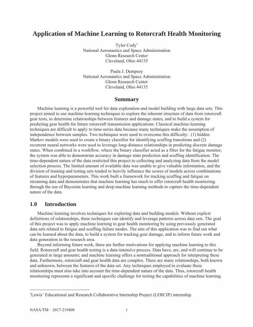
The data used in this project spanned multiple spiral bevel gear set (pinion and gear) tests. Tests were performed in the Spiral Bevel Gear Fatigue Test Rig at the NASA Glenn Research Center. A detailed description of this test facility is provided in References 1 and 2. The Spiral Bevel Gear Fatigue Test Rig is illustrated with a cross-sectional view in Figure 1. The facility operates as a closed-loop torque regenerative system, where the drive motor only needs enough power to overcome the losses within the system. The load is locked into the loop via a split shaft and a thrust piston that forces a floating helical gear axially into the mesh. The 100-hp drive motor supplies the test rig with rotation and overcomes loop losses via V-belts to the axially stationary helical gear.

Two sets of spiral-bevel gears, referenced as left and right when facing the gearboxes, are installed in the gearbox. The concave side of the pinion is always in contact with the convex side of the gear on both the left and right side. However, the pinion drives the gear in the normal speed reducer mode on the left side, while the pinion acts as a speed increaser on the right side.

Both gear sets are lubricated with oil jets pumped from an oil reservoir using qualified helicopter transmission oil. The oil drains from the gearbox, flows through an inductance-type in-line oil debris sensor, then flows past a magnetic chip detector. A strainer and a 3-μm filter capture any debris before the oil returns to the gearbox.

Facility operational parameters, torque, speed, and gearbox oil temperatures were collected every minute with a facility data acquisition (DAQ) system. A commercially available noncontact rotary transformer shaft-mounted torque sensor was used to measure torque during testing. Oil inlet, outlet, and fling-off temperatures were measured with thermocouples. The fling-off temperature was measured inside the gearbox where the oil was flung off of the gears at the out-of-mesh position.

Vibration, oil debris, torque, and speed data were also collected once every minute with Glenn’s research DAQ system, the Mechanical Diagnostic System Software (MDSS). The NASA MDSS system acquires, digitizes, and processes the tachometer pulses and accelerometer data. A new experiment is set up when a new gear set is installed on the left side of the test rig.

Figure 1.—Spiral Bevel Gear Fatigue Test Rig.

NASA/TM—2017-219408 3

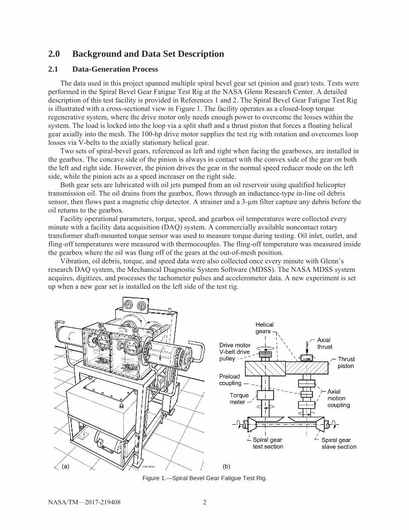
Figure 2.—Location of Mechanical Diagnostic System Software (MDSS) accelerometers.

Oil debris data were collected from an inductance-type oil debris sensor and a magnetic chip detector.

The inductance-type oil debris sensor was used to measure the ferrous debris generated during fatigue damage to the gear teeth. The MDSS recorded the number of particles and their approximate size on the basis of user-defined particle size ranges or bins. The user-defined average particle size for each bin was used to calculate the cumulative mass: the average particle diameter (for particles assumed to be spherical) was multiplied by the density of steel. Reference 3 has a detailed analysis of the oil debris data generated during testing.

Vibration data were measured with accelerometers installed on the right and left sides of the test rig pinion support housings, radially and vertically with respect to the pinion, as shown in Figure 2. Facing the gearboxes, the left gear set (pinion and gear) and right gear set (pinion and gear) accelerometers were referenced as such in the MDSS system. Speed was measured with optical tachometers mounted on the left pinion shaft and left gear shaft to produce a separate once-per-revolution tachometer pulse for the pinion and gears. Reference 4 provides additional details on the vibration data collected during these tests.

2.2 Gear Design

The gears tested were designed to represent a rotorcraft drive system gear mesh. To minimize scuffing and force a failure on the left-side gear set, several gear sets were super-finished (a process that improves gear surface and extends gear life) and installed on the right side of the gearbox (Ref. 5). Surface roughness improved by a factor of 4 on average after this process was applied.

2.3 Gear Set Failure Modes

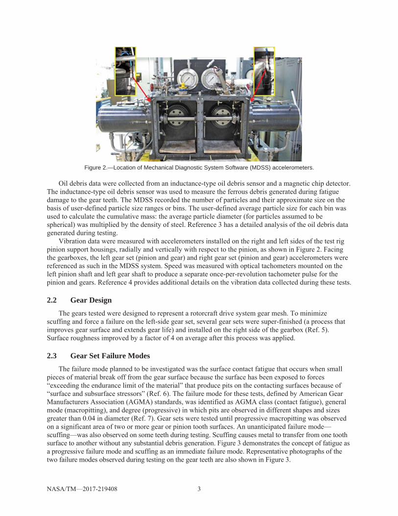
The failure mode planned to be investigated was the surface contact fatigue that occurs when small pieces of material break off from the gear surface because the surface has been exposed to forces “exceeding the endurance limit of the material” that produce pits on the contacting surfaces because of “surface and subsurface stressors” (Ref. 6). The failure mode for these tests, defined by American Gear Manufacturers Association (AGMA) standards, was identified as AGMA class (contact fatigue), general mode (macropitting), and degree (progressive) in which pits are observed in different shapes and sizes greater than 0.04 in diameter (Ref. 7). Gear sets were tested until progressive macropitting was observed on a significant area of two or more gear or pinion tooth surfaces. An unanticipated failure mode—scuffing—was also observed on some teeth during testing. Scuffing causes metal to transfer from one tooth surface to another without any substantial debris generation. Figure 3 demonstrates the concept of fatigue as a progressive failure mode and scuffing as an immediate failure mode. Representative photographs of the two failure modes observed during testing on the gear teeth are also shown in Figure 3.

NASA/TM—2017-219408 4

Figure 3.—Gear set failure modes.

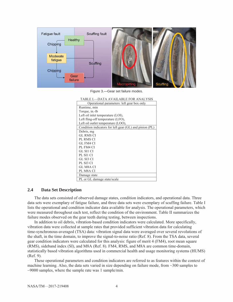
TABLE I.—DATA AVAILABLE FOR ANALYSIS

Operational parameters: left gear box only Runtime, min Torque, in.-lb Left oil inlet temperature (LOI), Left fling-off temperature (LFO), Left oil outlet temperature (LOO), Condition indicators for left gear (GL) and pinion (PL) Debris, mg GL RMS CI PL RMS CI GL FM4 CI PL FM4 CI GL SI1 CI PL SI1 CI GL SI3 CI PL SI3 CI GL M8A CI PL M8A CI Damage state PL or GL damage state/scale

2.4 Data Set Description

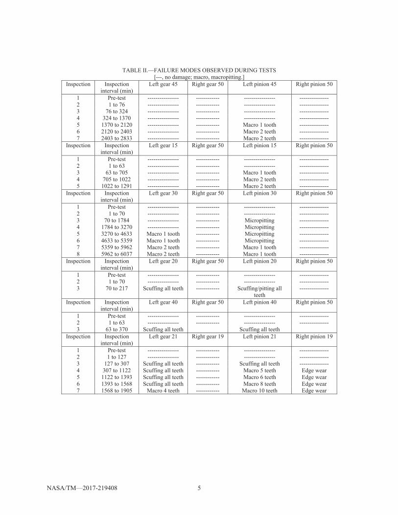
The data sets consisted of observed damage states, condition indicators, and operational data. Three data sets were exemplary of fatigue failure, and three data sets were exemplary of scuffing failure. Table I lists the operational and condition indicator data available for analysis. The operational parameters, which were measured throughout each test, reflect the condition of the environment. Table II summarizes the failure modes observed on the gear teeth during testing, between inspections.

In addition to oil debris, vibration-based condition indicators were calculated. More specifically, vibration data were collected at sample rates that provided sufficient vibration data for calculating time-synchronous-averaged (TSA) data: vibration signal data were averaged over several revolutions of the shaft, in the time domain, to improve the signal-to-noise ratio (Ref. 8). From the TSA data, several gear condition indicators were calculated for this analysis: figure of merit 4 (FM4), root mean square (RMS), sideband index (SI), and M8A (Ref. 8). FM4, RMS, and M8A are common time-domain, statistically based vibration algorithms used in commercial health and usage monitoring systems (HUMS) (Ref. 9).

These operational parameters and condition indicators are referred to as features within the context of machine learning. Also, the data sets varied in size depending on failure mode, from ~300 samples to ~9000 samples, where the sample rate was 1 sample/min.

NASA/TM—2017-219408 5

TABLE II.—FAILURE MODES OBSERVED DURING TESTS [---, no damage; macro, macropitting.]

Inspection Inspection interval (min)

Left gear 45 Right gear 50 Left pinion 45 Right pinion 50

1 Pre-test ---------------- ------------ ---------------- --------------- 2 1 to 76 ---------------- ------------ ---------------- --------------- 3 76 to 324 ---------------- ------------ ---------------- --------------- 4 324 to 1370 ---------------- ------------ ---------------- --------------- 5 1370 to 2120 ---------------- ------------ Macro 1 tooth --------------- 6 2120 to 2403 ---------------- ------------ Macro 2 teeth --------------- 7 2403 to 2833 ---------------- ------------ Macro 2 teeth ---------------



1 Pre-test ---------------- ------------ ---------------- --------------- 2 1 to 63 ---------------- ------------ ---------------- --------------- 3 63 to 705 ---------------- ------------ Macro 1 tooth --------------- 4 705 to 1022 ---------------- ------------ Macro 2 teeth --------------- 5 1022 to 1291 ---------------- ------------ Macro 2 teeth ---------------



1 Pre-test ---------------- ------------ ---------------- --------------- 2 1 to 70 ---------------- ------------ ---------------- --------------- 3 70 to 1784 ---------------- ------------ Micropitting --------------- 4 1784 to 3270 ---------------- ------------ Micropitting --------------- 5 3270 to 4633 Macro 1 tooth ------------ Micropitting --------------- 6 4633 to 5359 Macro 1 tooth ------------ Micropitting --------------- 7 5359 to 5962 Macro 2 teeth ------------ Macro 1 tooth --------------- 8 5962 to 6037 Macro 2 teeth ------------ Macro 1 tooth ---------------



1 Pre-test ---------------- ------------ ---------------- --------------- 2 1 to 70 ---------------- ------------ ---------------- --------------- 3 70 to 217 Scuffing all teeth ------------ Scuffing/pitting all

teeth ---------------



1 Pre-test ---------------- ------------ ---------------- --------------- 2 1 to 63 ---------------- ------------ ---------------- --------------- 3 63 to 370 Scuffing all teeth Scuffing all teeth



1 Pre-test ---------------- ------------ ---------------- --------------- 2 1 to 127 ---------------- ------------ ---------------- --------------- 3 127 to 307 Scuffing all teeth ------------ Scuffing all teeth --------------- 4 307 to 1122 Scuffing all teeth ------------ Macro 5 teeth Edge wear 5 1122 to 1393 Scuffing all teeth ------------ Macro 6 teeth Edge wear 6 1393 to 1568 Scuffing all teeth ------------ Macro 8 teeth Edge wear 7 1568 to 1905 Macro 4 teeth ------------ Macro 10 teeth Edge wear

NASA/TM—2017-219408 6

3.0 Approach 3.1 Introduction to Machine Learning

Machine learning is used in data analysis to automate analytical model building. The machine uses algorithms to learn from data iteratively to discover trends, identify patterns, and make predictions. This learning can be divided into two broad groupings: (1) supervised learning and (2) unsupervised learning (Ref. 10). In the typical case, supervised learning methods are used for building models for prediction, whereas unsupervised learning methods are used for data exploration.

In supervised learning, algorithms try to predict an output when given an input vector, which can come in the form of regression or classification. In supervised learning, a training data set is selected that has labeled target output data for given input data; then a model is trained to find the mapping function for this relationship. That is, supervised learning requires a labeled set of data.

In unsupervised learning, algorithms try to discover a good internal representation of the input. In some cases this is used to create a useful representation of the data for subsequent supervised learning tasks, such as methods to identify key features or parameters in the data. However, unsupervised learning techniques are also standalone tools that can explore patterns in data when the patterns to look for have not been explicitly defined.

Supervised and unsupervised learning define two ends of a spectrum. Many methods fall into a semisupervised category somewhere between the two that leverages the benefits of both learning techniques.

3.2 Classical Machine Learning

Several more classical machine-learning algorithms can be grouped effectively into one of a number of categories. The categories, which span supervised and unsupervised techniques, are described in the following list to broadly highlight common techniques used in machine learning.

Regression algorithms iteratively refine a modeling of relationships between variables. This refining is performed by minimizing a measure of error in the predictions made by the model. Common algorithms are linear, logistic, and stepwise regression.

Regularization algorithms penalize models on the basis of their complexity, thus selecting features internally as part of the model-building process. They are typically extensions of regression methods, of which two popular types are ridge regression and lasso regression.

Clustering algorithms explore inherent structures in the input data to group them by their commonalities. These usually involve some form of a distance calculation between points; a prime example is a k-means algorithm.

Decision tree algorithms base decision models on the values of attributes in the input data. A given input datum follows a path down the tree until a prediction is reached at a leaf node. Decision tree methods are quick to build and fast in prediction.

Ensemble algorithms leverage independently trained weaker models by using them together to create a more powerful, robust model. Popular ensemble methods include random forests and gradient-boosted forests, which leverage the speed of decision trees by using large numbers of these trees together in modeling.

3.3 Machine Learning and Time-Series Analysis

From the onset, gear health monitoring was known to be a time-dependent problem. That is, successive samples in a data set cannot be assumed to be independent. However, many of the classical machine-learning techniques make this assumption. In evaluating a sequence of points, a given tempera-ture at time-step 0 may have a completely different significance than the same temperature at time-step 100. The algorithms listed in Section 3.2 are unable to capture this nature of the data out of the box.

NASA/TM—2017-219408 7

Initially, attempts were made to build memory into the data. For example, the debris feature of the data sets represented the total debris accumulated. Thus, there is a degree of memory between samples. However, finding similar solutions for temperature, torque, or condition indicators proved fruitless. Tracking statistics such as moving averages and moving variances could not justly capture the data. Initial attempts to apply classical methods to these constructed features showed little to no significant change in predictive power.

A broader search of algorithms ensued with a particular focus on sequence classification and prediction. Two approaches that solved the time dependency issue and also offered a more robust method of modeling sequences arose in the form of a state-based approach via hidden Markov models (HMM, Ref. 11) and in the form of a neural network (NN) approach via recurrent neural networks (RNNs, Ref. 10).

HMMs are probabilistic models of time-series data (Ref. 11). In a Markov process, the state at time t + 1 depends only on the state at time t. HMMs extend this principle by including additional hidden states that are not directly observable. (A detailed explanation of the math and schematics behind HMMs is beyond the scope of this report.) The ability of HMMs to model full sequences solves the issue of time dependence; however, it is not obvious how to interpret the hidden states that the model generates. Regardless, HMMs are flexible in their use and can be used for future sequence prediction and classification in time-series data if they are trained on a fixed sequence size. The ability to learn the probability of a fixed sequence can be used in building a binary temporal classifier to identify scuffing transitions. Scuffing transitions are identifiable periods in data sets where scuffing is initiated. In the data sets available they are brief periods of 5 to 10 samples. Specifics on implementing this classifier will be discussed later in this report.

NNs are models that mimic properties of the neurons in the brain to form powerful predictive tools capable of mapping nonlinear relationships. They consist of layers of neurons that are interconnected via weights. These weights act on an input vector to transform it as it passes through hidden neuron layers to form an output vector. Training in an NN involves calculating and tuning these weights to create the mapping function. Although the exact architecture of these networks varies, traditional NNs make the same assumption of independence between samples that limits classical machine-learning algorithms.

RNNs overcome this shortcoming of NNs. In a simplified sense, RNNs are NNs with loops in them that allow information to persist. They use a hidden layer that is recurrently connected to itself, allowing memory to pass between samples within a sequence. (A detailed explanation of the math and schematics behind RNNs is beyond the scope of this report.) Not only do RNNs account for the time-dependent nature of the gear health data, but also they allow for modeling patterns by using a variable dependence on sequence length. That is, while the persistence of memory in HMMs is fixed, RNNs can be tuned to drop out, or “forget,” past samples similar to how neurons in the brain forget information when it is not used (Ref. 10). Because of this added flexibility in modeling a time series, RNNs were chosen to build fatigue monitors that returned a probability distribution of current and future damage states. Specifics on implementing this classifier will be discussed later in this report.

3.4 Unsupervised Learning and Data Exploration With Time-Series Data

Data exploration in machine learning typically involves the deployment of unsupervised learning methods. A majority of the well-defined unsupervised learning methods, however, involve clustering or vector decomposition. Both of these techniques have limited application—at best—in time-dependent data because they rely on the assumption of independence between samples.

The best method found during this project to explore the structure of the data and relationships among features and damage states was to collect data during the model selection process. In machine learning, the model selection process involves iterating over possible combinations of algorithms, features, and hyperparameters to identify the optimal model. Often this process is fully automated with a final selection step that either combines top models or uses a winner-take-all mentality and chooses the best performing model exclusively.

NASA/TM—2017-219408 8

This model-building process can be modified slightly to encompass data selection. By collecting data about the performance of each combination of features and hyperparameters while searching for the optimal model, a researcher can generate large amounts of information about the data set itself. Beyond having the ability to explore this acquired information by factors such as accuracy, complexity of model, true positive/true negative/false positive/false negative rates, and robustness to sensitivity analysis, the researcher has also created a data set that has independence between samples and thus can apply unsupervised learning techniques to the results of the model selection process.

4.0 Methods and Implementation of Monitor System 4.1 System Architecture

From the onset it was clear that the available data sets would give a limited representation of the parameter space. Although the quality of each individual set was not constraining, the variety of sets available was seen as a potential issue, and ultimately it became one. Thus, instead of fitting models to the data available, the construction of the monitor system was done from a top-down, conceptual approach. That is, design decisions were made with respect to the nature of the problem space, as opposed to optimizing specifically to the data on hand. This was done not only as an attempt to reduce overfitting due to the lack of variety in available data but to stay true to the exploratory nature of the project.

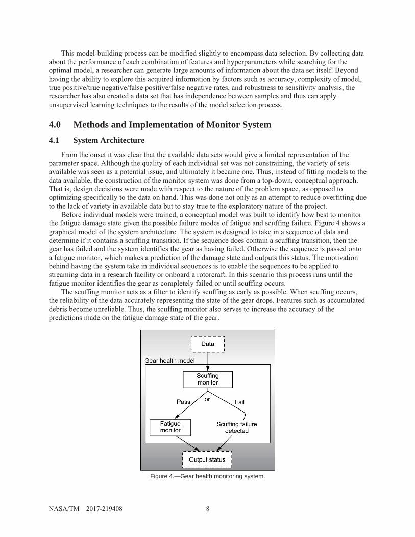
Before individual models were trained, a conceptual model was built to identify how best to monitor the fatigue damage state given the possible failure modes of fatigue and scuffing failure. Figure 4 shows a graphical model of the system architecture. The system is designed to take in a sequence of data and determine if it contains a scuffing transition. If the sequence does contain a scuffing transition, then the gear has failed and the system identifies the gear as having failed. Otherwise the sequence is passed onto a fatigue monitor, which makes a prediction of the damage state and outputs this status. The motivation behind having the system take in individual sequences is to enable the sequences to be applied to streaming data in a research facility or onboard a rotorcraft. In this scenario this process runs until the fatigue monitor identifies the gear as completely failed or until scuffing occurs.

The scuffing monitor acts as a filter to identify scuffing as early as possible. When scuffing occurs, the reliability of the data accurately representing the state of the gear drops. Features such as accumulated debris become unreliable. Thus, the scuffing monitor also serves to increase the accuracy of the predictions made on the fatigue damage state of the gear.

Figure 4.—Gear health monitoring system.

NASA/TM—2017-219408 9

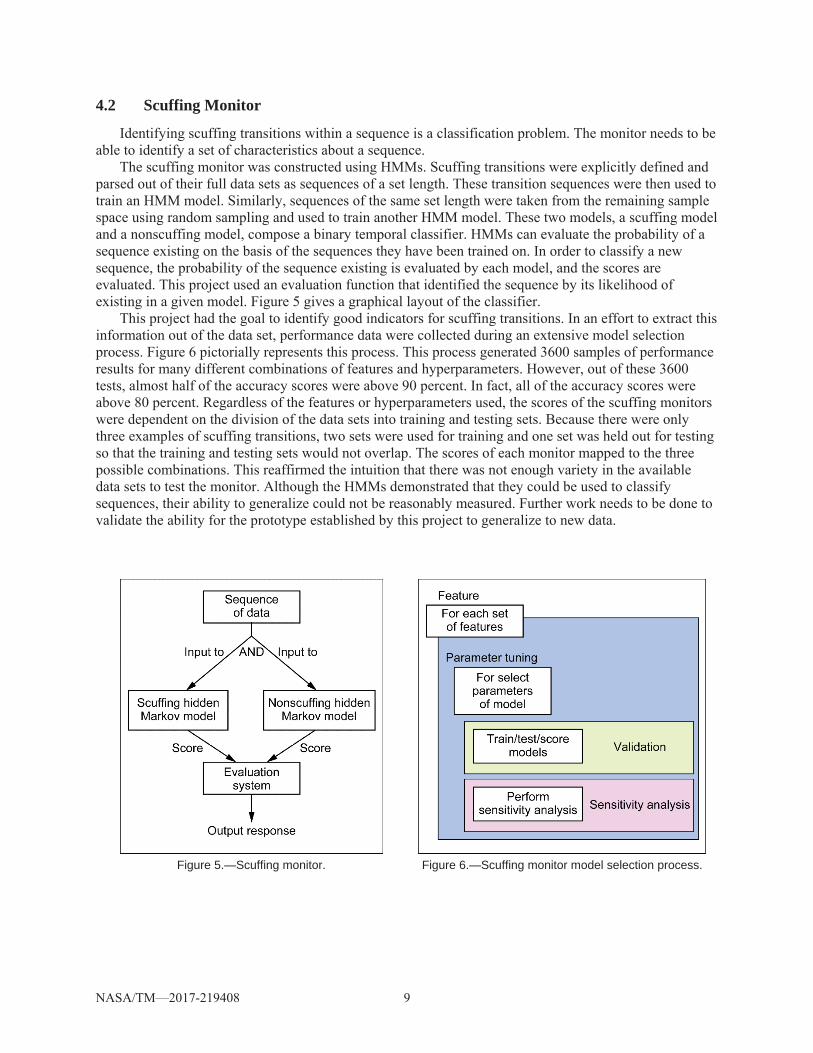
4.2 Scuffing Monitor

Identifying scuffing transitions within a sequence is a classification problem. The monitor needs to be able to identify a set of characteristics about a sequence.

The scuffing monitor was constructed using HMMs. Scuffing transitions were explicitly defined and parsed out of their full data sets as sequences of a set length. These transition sequences were then used to train an HMM model. Similarly, sequences of the same set length were taken from the remaining sample space using random sampling and used to train another HMM model. These two models, a scuffing model and a nonscuffing model, compose a binary temporal classifier. HMMs can evaluate the probability of a sequence existing on the basis of the sequences they have been trained on. In order to classify a new sequence, the probability of the sequence existing is evaluated by each model, and the scores are evaluated. This project used an evaluation function that identified the sequence by its likelihood of existing in a given model. Figure 5 gives a graphical layout of the classifier.

This project had the goal to identify good indicators for scuffing transitions. In an effort to extract this information out of the data set, performance data were collected during an extensive model selection process. Figure 6 pictorially represents this process. This process generated 3600 samples of performance results for many different combinations of features and hyperparameters. However, out of these 3600 tests, almost half of the accuracy scores were above 90 percent. In fact, all of the accuracy scores were above 80 percent. Regardless of the features or hyperparameters used, the scores of the scuffing monitors were dependent on the division of the data sets into training and testing sets. Because there were only three examples of scuffing transitions, two sets were used for training and one set was held out for testing so that the training and testing sets would not overlap. The scores of each monitor mapped to the three possible combinations. This reaffirmed the intuition that there was not enough variety in the available data sets to test the monitor. Although the HMMs demonstrated that they could be used to classify sequences, their ability to generalize could not be reasonably measured. Further work needs to be done to validate the ability for the prototype established by this project to generalize to new data.

Figure 5.—Scuffing monitor. Figure 6.—Scuffing monitor model selection process.

NASA/TM—2017-219408 10

4.3 Fatigue Monitor

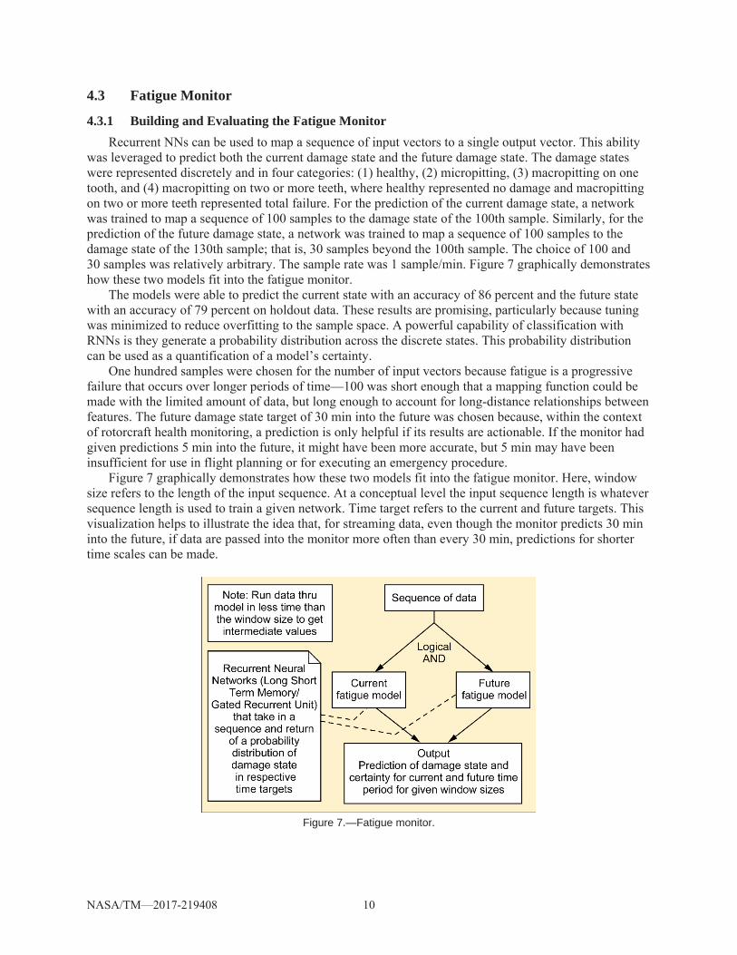
4.3.1 Building and Evaluating the Fatigue Monitor Recurrent NNs can be used to map a sequence of input vectors to a single output vector. This ability

was leveraged to predict both the current damage state and the future damage state. The damage states were represented discretely and in four categories: (1) healthy, (2) micropitting, (3) macropitting on one tooth, and (4) macropitting on two or more teeth, where healthy represented no damage and macropitting on two or more teeth represented total failure. For the prediction of the current damage state, a network was trained to map a sequence of 100 samples to the damage state of the 100th sample. Similarly, for the prediction of the future damage state, a network was trained to map a sequence of 100 samples to the damage state of the 130th sample; that is, 30 samples beyond the 100th sample. The choice of 100 and 30 samples was relatively arbitrary. The sample rate was 1 sample/min. Figure 7 graphically demonstrates how these two models fit into the fatigue monitor.

The models were able to predict the current state with an accuracy of 86 percent and the future state with an accuracy of 79 percent on holdout data. These results are promising, particularly because tuning was minimized to reduce overfitting to the sample space. A powerful capability of classification with RNNs is they generate a probability distribution across the discrete states. This probability distribution can be used as a quantification of a model’s certainty.

One hundred samples were chosen for the number of input vectors because fatigue is a progressive failure that occurs over longer periods of time—100 was short enough that a mapping function could be made with the limited amount of data, but long enough to account for long-distance relationships between features. The future damage state target of 30 min into the future was chosen because, within the context of rotorcraft health monitoring, a prediction is only helpful if its results are actionable. If the monitor had given predictions 5 min into the future, it might have been more accurate, but 5 min may have been insufficient for use in flight planning or for executing an emergency procedure.

Figure 7 graphically demonstrates how these two models fit into the fatigue monitor. Here, window size refers to the length of the input sequence. At a conceptual level the input sequence length is whatever sequence length is used to train a given network. Time target refers to the current and future targets. This visualization helps to illustrate the idea that, for streaming data, even though the monitor predicts 30 min into the future, if data are passed into the monitor more often than every 30 min, predictions for shorter time scales can be made.

Figure 7.—Fatigue monitor.

NASA/TM—2017-219408 11

4.3.2 Notes on Network Structure and Optimization RNNs can take many forms. In an effort to be explicit, in this section, the authors describe the

specific structure of the two networks developed. The basic architecture of the network consisted of five layers: one input layer, three hidden layers, and one output layer. The three hidden layers had the capability for dropout. Dropout is a mechanism that RNNs use to control the depth of their memory. The performance of an NN is highly dependent on extensive hyperparameter tuning. So that the dependence of the structure of the network on the sample space would be minimized, only a handful of parameters were tuned. The networks had the option of choosing between long short-term memory (LSTM) layers (Ref. 10) and gated recurrent unit (GRU) layers (Ref. 12) for the structure of the hidden layers. The number of neurons per layer were allowed to vary among 32, 64, 128, and 256; and the proportion of neurons to drop out between each hidden layer was allowed to vary on a uniform distribution from 0 to 1.

The favored structures for the current and future damage state predictor were identical. Both networks favored similar structures under optimization, with the number of neurons in the hidden layers being 64, 256, and 32 in order from the input layer to the output layer. The dropout proportions varied between 0.35 and 0.50. The LSTM layers outperformed the GRU layers for both models. Similar to the results for HMMs, it is not obvious how to interpret the results of the optimization. The dropout proportion nearing 0.50 indicates that the optimized layers dropped about half of the input units that they received. Although this information is interesting, interpreting the structure of the model is ill-defined. That is, drawing significance from the network architecture requires a degree of speculation. Furthermore, this model is optimized to the available data. If the available data lack variety, then the structure of the optimized models may not generalize well to the parameter space.

4.3.3 Notes on Techniques for Implementation In this subsection, in an effort to inform future work, the authors describe a few of the techniques

used and the limitations that were faced in building the RNNs. When one is working with small data set sizes, interpolation techniques can be helpful in up-sampling to increase the training set size. The idea is to use interpolation techniques to create synthetic training sets that are dissimilar enough from the original training sets that they are helpful in fitting the network but that are not so dissimilar that they are unrealistic. Two techniques used in this project to accomplish this were moving averages for mean and variance. An issue faced during this project was the training time required to fit a network. Because there was no access to the graphics processing units (GPUs), the optimization of matrix calculations was limited. This project instead used central processing units (CPUs) to parallelize network training so that during optimization multiple network structures could be evaluated simultaneously. A similar technique was used to increase the speed of the k-fold cross-validation. Although the model selection process for the scuffing monitor of iterating over combinations of features and hyperparameters was satisfactory for tuning the HMMs, this project used Bayesian search techniques for tuning the fatigue model networks to dramatically reduce optimization time.

4.4 Full Gear Health Monitoring System

After implementing both monitors, the gear health monitoring system could be realized. The system takes in input data of a given batch size. For demonstration, the batch size was chosen to be one. This means that data are passed into the system every minute. Once data have been streaming for 20 min, the scuffing monitor can classify a sequence every minute on the basis of the previous 20 min. Once data have been streaming for 100 min, the fatigue monitor can predict damage states every minute on the basis of the previous 100 min. If a scuffing transition is found, the system raises a flag to indicate gear failure. The system outputs a predicted current damage state, a predicted future damage state, an assessment of scuffing for the current sequence, an assessment of scuffing in any of the past sequences, and a probability distribution for each damage state prediction (current and future).

NASA/TM—2017-219408 12

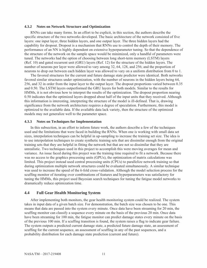
Figure 8.—Monitor system output. (a) Predicted and actual current damage states for the fatigue data set.

(b) Predicted and actual future damage states for the fatigue data set. (c) Certainty of model in current damage state prediction over time. (d) Certainty of model in future damage prediction over time.

For demonstration purposes this system was used to evaluate an example data set. The results are plotted in Figure 8.

Figures 8(a) and (b) are plots of the predicted and actual damage state of the test. Figure 8(a) uses the higher accuracy model and displays the prediction of the current damage state. Figure 8(b) uses the lower accuracy model and displays the prediction of the future damage state. Damage states of 1, 2, 3, and 4 correspond to healthy, micropitting, macropitting on one tooth, and macropitting on two or more teeth, respectively. Figures 8(c) and (d) show the probability distributions of each damage state prediction for both models. Each time that a sequence was passed through the network, the model made its state prediction by comparing the probabilities of each class.

The data set that was fed through the system exhibited fatigue failure. In the predicted damage state plots, where the points do not overlap, an error had been made by the model. It is visually clear that the future damage state was more difficult for the system to predict. Namely, the system was naïve to the fact that damage states only increase. However, logic controls could be implemented to minimize these errors.

When taken together, both the current and future prediction plots (Figs. 8(c) and (d)) showed the greatest error and uncertainty between ~400 and ~800 min. Notably this is the period where the gear was transitioning to a fatigue failure (two or more teeth with macropitting). This might indicate that the four states used may have been too broad to classify this transition to failure. Once the gear had failed, however, the model was certain in its predictions of failure.

These visual representations help demonstrate the output of the system and how the system might perform in a research or onboard setting. Although not relevant to the data set displayed, the system also recorded a local and global indicator of a scuffing transition, where local relates to a given sequence and global relates to an entire data set.

NASA/TM—2017-219408 13

5.0 Conclusions 5.1 Synopsis of Project

Machine learning involves techniques for data exploration and model building. These techniques can identify and leverage patterns across data sets without the need for relationships to be defined explicitly. The goal of this project was to apply machine learning to gear health monitoring using previously generated data sets related to fatigue and scuffing failure modes. The aim of this application was to find out what can be learned about the data, to build a system for tracking gear damage, and to inform future work and data generation in the research area. From the onset, it was clear that the available data were limited; thus, the machine learning was analyzed with an emphasis at the conceptual level.

The project started by surveying the classical machine-learning algorithms; however, many of these make the assumption of independence between samples—a restrictive assumption in time-series analysis. Ultimately, a combination of hidden Markov models (HMMs) and recurrent neural networks (RNNs) were used for their ability to capture patterns across sequences. These two techniques were used to construct a framework for tracking gear health where a binary classifier acted as a filter for feeding data into the fatigue-monitoring networks, and this system served to accurately track fatigue damage over time.

HMMs allow patterns of fixed sequence lengths to be modeled. This ability was leveraged using sample sequences of scuffing transitions to build a binary temporal classifier. A lack of data variety made the accuracy of the classifier dependent on the division of training and testing sets, and although accuracies as high as 98 percent were achieved, the lack of data variety suggests that the models were severely overfitted. If fatigue models could identify when scuffing has occurred, they could better leverage expertise knowledge in fatigue monitoring, namely the debris sensor data.

RNNs, which allow for modeling patterns using a variable dependence on sequence length, were used to build fatigue monitors that returned a probability distribution of current and future damage states. Accuracy of prediction was 86 percent for the current damage state and 79 percent for the future damage state when three data sets were used (expanded to nine sets for training using interpolation techniques).

Because of the limited representation of the available data sets in the parameter space by, minimal tuning was performed on the models to reduce overfitting. This limitation also restricted the ability to explore the data set via the model selection process because results were noticeably biased by the division of testing and training data.

5.2 Discussion and Future Work

This work demonstrates that machine learning has much to offer rotorcraft health monitoring. Bayesian learning and deep machine learning account for the time-dependent nature of the data. These two modeling techniques showed notable accuracy in tracking the gear damage state, as well as promise in data set exploration. This project used these techniques to develop a framework for monitoring gear health that is grounded in the assumptions of the models and the data sets.

Although this project was able to demonstrate a degree of viability of these techniques, the available data sets lacked enough variety to test the capability of the models, monitors, and system to generalize to new data. In extreme cases, the results of testing were dependent on the division of training and testing sets. Also, the number of data sets limited the amount of optimization. In time-series analysis, unsupervised learning is limited, and data exploration is done primarily through observing the results of fine tuning the models and selecting features. Tuning the models was limited in building the fatigue monitor and impossible in building the scuffing monitor. In future work, feeding more data into this framework could validate the system and offer insight into the inherent structure of the data.

There are several ways that a larger repository of data sets could change the approach taken in this project while still using the system developed in this project. The RNNs were only minimally tuned because the parameter space does not represent the available data. With more freedom in optimization processes, the networks might perform better with a variety of different types of layers, with more or less

NASA/TM—2017-219408 14

layers, and/or with different optimization functions. Also, with more data, it might be feasible to investigate fatigue as continuous (as opposed to discrete). With a slight adjustment, the networks could be used to predict a value for damage as opposed to a category. Also, an unsatisfied curiosity of this project was the dependence of the predicted state on the input sequence length. Given more time, processing power, and data, it would be appropriate to vary the number of past data points that the fatigue and scuffing monitors have and to observe the output. For example, maybe 100 min is a good length of time for predicting current damage but not future damage. Or maybe 20 min is too long or short a time span to accurately identify a scuffing transition.

The suggested direction for future work is to apply the framework developed in this project to a sample space more representative of the parameter space to solidify the efficacy of the model’s predictive power and harness its ability for data exploration. Beyond this, it would be interesting to generalize and automate data processing so that the system could generate live predictions on streaming data from a test rig.

References 1. Handschuh, Robert F.: Thermal Behavior of Spiral Bevel Gears. NASA TM–106518, 1995.

http://ntrs.nasa.gov 2. Handschuh, Robert F.: Testing of Face-Milled Spiral Bevel Gears at High-Speed and Load.

NASA/TM—2001-210743, 2001. http://ntrs.nasa.gov 3. Dempsey, Paula; and Handschuh, R.F.: Detection of Spiral Bevel Gear Damage Modes Using Oil

Debris Particle Distributions. Joint Conference: MFPT 2015 and ISA’s 61st International Instrumentation Symposium, ISA Volume 507, 2015.

4. Dempsey, Paula J.: Investigation of Spiral Bevel Gear Condition Indicator Validation via AC–29–2C Using Damage Progression Tests. NASA/TM—2014-218384, 2014. http://ntrs.nasa.gov

5. Niskanen, Paul W.; Hansen, Bruce; and Winkelmann, Lane: Scuffing Resistance of Isotropic Superfinished Precision Gears. Gear Solutions, 2008. http://www.gearsolutions.com/article/ detail/5810/scuffing-resistance-of-isotropic-superfinished-precision-gears Accessed Dec. 1, 2016.

6. Dudley, Darle W.; and Townsend, Dennis P.: Dudley’s Gear Handbook. McGraw-Hill, New York, NY, 1991.

7. American Gear Manufacturers Association: Appearance of Gear Teeth—Terminology of Wear and Failure. AGMA 1010–E95, 2014.

8. Martin, H.R.: Statistical Moment Analysis as a Means of Surface Damage Detection. Proceedings of the 7th International Modal Analysis Conference, Society for Experimental Mechanics, Schenectady NY, 1989, pp. 1016–1021.

9. Stewart, R.M.: Some Useful Data Analysis Techniques for Gearbox Diagnostics. Institute of Sound and Vibration Research Report MHM/R/10/77, 1977.

10. Safari, Pooyan: Deep Learning for Sequential Pattern Recognition. Master Thesis, Technical University of Munich, 2013.

11. Rabiner, Lawrence R.: A Tutorial on Hidden Markov Models and Selected Applications in Speech Recognition. Proc. IEEE, vol. 77, no. 2, 1989, pp. 257–286.

12. Chung, Junyoung, et al.: Empirical Evaluation of Gated Recurrent Neural Networks on Sequence Modeling. arXiv:1412.3555, Cornell University Library, Ithaca, NY, 2014.

application of machine learning to rotorcraft health ... · application of machine learning to...

Documents