application of non-local approaches for …momrg.cecs.ucf.edu/theses/nguyent_him.pdf · methods...

i

APPLICATION OF NON-LOCAL APPROACHES FOR PREDICTING THE

RESPONSE OF V-NOTCH UNDER THERMOMECHANICAL FATIGUE

LOADING

by

TRUNG V. NGUYEN

A Thesis submitted in partial fulfillment of the

requirements for the Honors in the Major Program

in Aerospace Engineering in the College

Engineering and Computer Science and in the

Burnett Honors College at the University of Central

Florida

Orlando, Florida

Spring Term 2013

Thesis Chair: Dr. Ali P. Gordon

ii

Abstract

The topic of this thesis is the construction of a formula to approximate stress-strain

responses at notches under thermomechanical fatigue (TMF) loading. The understanding of

material behavior of the V-notched component which experiences TMF is important to the

mechanical industries where V-notched structures are often utilized. In such applications, it is

crucial that the designers be able to predict the material behavior; therefore, the purpose of this

research is to examine and to model the precise effects a stress concentration will have on a

specimen made of a generic Ni-base superalloy. The effects of non-isothermal loading will be

studied, and it is the goal of this research to formulate an extension of Neuber’s rule appropriate

for TMF which is to approximate the temperature range with a single value, T*. One strategy to

extend Neuber’s rule, which relies on Finite Element Modeling (FEM), Bilinear Kinetic

Hardening Model (BKIN), and test data, will be used to predict the stress-strain behavior at the

notch of a thin plate subjected to axial loading. In addition, the CHABOCHE model will be

utilized in the FEA to have the highest fidelity to material response at high temperatures.

Parametric study of the FEA simulations will be employed to determine the correlation between

the Neuber hyperbola, temperature range, stress concentration, the nominal stress, and the

temperature cycling. Using the Neuber hyperbola and simplified constitutive model (i.e., bilinear

kinematic strain hardening), the stress-strain solutions of the specimen will be calculated and

compared to analytical results.

iii

Dedications

For my family whose love and supports help me to achieve many great accomplishments.

iv

Acknowledgments

I would like to express the deepest appreciation to my Thesis Chair, Dr. Ali P. Gordon,

who provides technical supports and guides me through my undergraduate study. In addition, Dr.

Gordon’s inspiration in doing research has motivated me to take my education to the graduate

level. Without the help from Dr. Gordon, this research would not be feasible. I would also like to

thank the graduate research assistants in the Mechanics of Materials Research Group at UCF.

Scott Keller helped me to expand my knowledge in mechanics of material field. Calvin Stewart

supported me in writing and developing ANSYS codes.

I would also like to thank my family for their continuous support throughout my study.

By encouraging and providing physical supports, they help me to accomplish many great

achievements in my life.

v

Table of Contents

1. Introduction .............................................................................................................................................. 1

2. Literature Review ..................................................................................................................................... 3

2.1 Materials ....................................................................................................................................... 3

2.2 Neuber's Rule ................................................................................................................................ 6

2.3 Review Modeling ......................................................................................................................... 7

2.3.1 BKIN model .......................................................................................................................... 7

2.3.2 CHABOCHE model ............................................................................................................ 10

2.4 Thermomechanical Fatigue ........................................................................................................ 18

2.5 Hypotheses.................................................................................................................................. 20

3. Numerical Simulation ............................................................................................................................ 23

3.1 Specimen Design ........................................................................................................................ 23

3.2 Formula Development ................................................................................................................ 24

4. Results and Discussion........................................................................................................................... 28

5. Conclusions ............................................................................................................................................ 32

6. Future Work ........................................................................................................................................... 33

Appendix ..................................................................................................................................................... 35

ANSYS code .......................................................................................................................................... 35

References ................................................................................................................................................... 41

vi

List of Figures

Figure 1: Temperature dependence of yield and ultimate strengths of generic Ni-base superalloy ............. 3

Figure 2a & 2b & 2c: Temperature dependence of elastic modulus, tangent modulus, and yielding stress

of the generic material .................................................................................................................................. 5

Figure 3: Interception of stress strain curve and σε total .............................................................................. 7

Figure 4: Stress-strain behavior of BKIN ..................................................................................................... 8

Figure 5a & 5b: The difference between the material behaviors of CHABOCHE and BKIN model ........ 12

Figure 6: Relationship between BKIN model and CHABOCHE model .................................................... 13

Figure 7: CHABOCHE model with varying γ ............................................................................................ 14

Figure 8: BKIN model and CHABOCHE with nonzero γ .......................................................................... 15

Figure 9a & 9b: Stress- Strain Behaviors of 6 Temperature Profiles using CHABOCHE Model .............. 17

Figure 10 a & 10b: Relationship between applied load and temperature in in-phase and out-phase case .. 19

Figure 11: BKIN model used to approximate the material behavior .......................................................... 21

Figure 12: Applied Pressure intercepts Yielding Stress at Yield Temperature........................................... 22

Figure 13 Specimen Constraints ................................................................................................................. 23

Figure 14: Von-Mises stress distribution .................................................................................................... 24

Figure 15: Parametric study on the combination of parameters in the right hand side of equation (12) .... 26

Figure 16a & 16b : Analytical stress-strain curve and ANSYS stress-strain curve for in-phase and out-

phase cases .................................................................................................................................................. 30

vii

Nomenclature

α Back Stress

ϵelastic, ϵplastic, ϵtotal Elastic, plastic, total strain, respectively

ρ Notch root radius

σ, σy Engineering stress, yielding stress

γi Recall term for non-linear effect in CHABOCHE

model

a Notch Angel

C1, C2 Constants in CHABOCHE model

d Distance between bottom of plate and tip of v-notch

E1,E2 Elastic and plastic modulus, respectively

h Thickness of the plate

j Interception of tangent modulus and y-axis

Kt Stress concentration factor

rn Notch radial location

S Nominal stress at the notch

t Notch depth

1

1. Introduction

Industrial gas turbine blades must be designed to operate under high temperature and

severe mechanical loads which cycle based on the workload of the machine. These conditions

are known as thermomechanical fatigue (TMF). In application, designers usually incorporate

small divots to the leading edge of the blade for cooling purpose. In most cases, these features

act as stress concentrations where plasticity can localize. Consequently, notches serve as sites for

crack initiation and reduce the fatigue life of component (Dowling 1979). It, therefore, is

important to capture the maximum stress (σmax), stress range (∆σ), elastic/plastic strain range (∆ϵ)

localized at the notch root. In recent years, several non-local shakedown methods have been

developed to approximate the distribution of stress caused by plastic flow in a zone of the stress

concentration. These models are limited to isothermal conditions only. Among them are the

methods established by Neuber (Neuber 1961) and Molinka and Glinka (Monlinski K.; Glinka

G. n.d.). With the aid of constitutive models, such as the Bilinear Kinematic Hardening (i.e.,

BKIN) model or the Nonlinear Kinematic Hardening (i.e, CHABOCHE) model, these local

approximation methods have excellent prediction of material response at high temperature. The

current research addresses extending a non-local method to non-isothermal conditions. This

investigation develops a formulation for the equivalent isothermal temperature, T*, which can be

used to predict notch tip response under non-isothermal conditions. This equivalent temperature

can be used to calculate the elastic and tangent modulus of BKIN model while compensating for

the BKIN’s inaccuracy in TMF. Based on these results, this effort develops a method to help

2

engineers approximate the critical stress-strain responds at the notch tip without the use of the

finite element method. The second chapter of this research will review material properties of

generic and material models that are used in the finite element analysis (i.e., FEA). The third

chapter of this thesis will discuss the set up of the FEA and the derivation of formula which

yields T*. Finally, a discussion on the final result will be made in chapter fourth and fifth, and a

conclusion can be drawn based on this result in chapter sixth.

3

2. Literature Review

2.1 Materials

The temperature in the combustion chamber of gas turbine can reach 1300oC before it is

blown into the turbine. By coating these blades and using notched structures, the temperature that

they have to withstand drops to the range of 750oC - 950

oC (Albeirutty H. M.; Alghamdi S. A.;

Najjar S. Y. 2004). Because of these extreme temperature and load, Ni base superalloy, which is

designed for long term mechanical exposure, are excellent candidates for the material of the

turbine blade material. These solids have high strength, and good corrosion/heat resistance;

therefore, they are used widely in gas turbine and other machines subjected to fluctuated

temperature and moisture environment. For a generic material, the temperature dependence of

yield and tensile strengths are shown in Figure 1 (Miskovic Z.; Janovic M.; Gligic M.; Likic B.

n.d.).

Figure 1: Temperature dependence of yield and ultimate strengths of generic Ni-base

superalloy

4

The temperature dependent of elastic modulus, tangent modulus, and yielding stress are found

using history data.

(a)

(b)

y = -0.001x4 + 4.174x3 - 3954.x2 + 2E+06x + 2E+08R² = 0.997

0

50

100

150

200

250

300

350

400

0 200 400 600 800 1000 1200 1400

Elas

tic

mo

du

lus

(MP

a)

Temperature (K)

Elastic modulus vs. Temperature

y = -0.435x4 + 949.1x3 - 70735x2 + 2E+08x + 8E+10R² = 0.916

0

20000

40000

60000

80000

100000

120000

0 200 400 600 800 1000 1200 1400

Tan

gen

t M

od

ulu

s (M

pa)

Temperature (K)

Tangent Modulus vs. Temperature

5

(c)

Figure 2a & 2b & 2c: Temperature dependence of elastic modulus, tangent modulus, and

yielding stress of the generic material

by interpolating the data, the equations for elastic and tangent modulus as function s of

temperature are

𝐸𝑒𝑙𝑎𝑠𝑡𝑖𝑐 = −0.001𝑇4 + 4.174𝑇3 − 3954𝑇2 + 2 ∗ 106𝑇 + 2 ∗ 108 (1)

𝐸𝑇 = −0.435𝑇4 + 949.1𝑇3 − 70735𝑇2 + 2 ∗ 108𝑇 + 8 ∗ 1010 (2)

𝜎𝑦𝑖𝑒𝑙𝑑 = −0.001𝑇4 + 3.618𝑇3 − 3369𝑇2 + 1 ∗ 106𝑇 + 2 ∗ 108 (3)

The material microstructure consists of γ-solid solution matrix and γ’-intermetallic precipitate

phase. A Cuboidal precipitates in the material are bimodally distributed with the matrix phase

(Jovanovic M. T.; Miskovic Z.; Lukic B. 1998), and high Cr-content imparts a high oxidation

y = -0.001x4 + 3.618x3 - 3369.x2 + 1E+06x + 2E+08R² = 0.991

0

50

100

150

200

250

300

350

400

0 200 400 600 800 1000 1200 1400

Yie

ldin

g St

ress

(M

Pa)

Temperature (K)

Temperature Dependence of Yielding Stress

6

resistance to the material (Nazmy M. Y.; Wuthrich C. 1983). As a result, this generic material

has considerable stiffness and creep resistance (Gordon. et al., 2008)

Table 1: IN939 Compositions, wt%

C Cr Co W Mo Nb Ta Ti Al Zr B Ni

0.15 22.4 19.0 2.0 … 1.0 1.4 3.7 1.9 0.1 0.01 Bal

2.2 Neuber's Rule

Neuber’s rule assumes that stress and strain solutions at the notch root can be expressed

as nominal elastic stress and strain response (S and e, respectively) and nominal, theoretical

stress concentration factor (Kt). Upon yielding at the notch tip, the stress concentration can be

approximated as

𝐾𝑡 = 𝐾𝜎𝐾𝜀 (4)

by assuming plastic deformation happens at the notch only, the product of stress and strain at the

notch is found to be

𝐾𝑡𝑆 2

𝐸= 𝜎𝜖 (5)

where E is the elastic modulus, and 𝜖 is the sum of elastic strain and plastic strain. The solution

to Neuber’rule is the intersection of the Neuber hyperbola and the tensile curve as in Fig. 3

(Gordon Ali P.; Eric P. Williams; Michael Schulist 2008)

7

Figure 3: Interception of stress strain curve and σε total

Neuber’s rule provides local notch root response on the basic of tensile behavior and the stress

concentration factor, kt. However, it is not applicable for non-isothermal condition.

2.3 Review Modeling

2.3.1 BKIN model

The equation that approximates the stress-strain solution at the notch in this research is

developed based on the rate independent Bilinear Kinematics Hardening, BKIN, model. This

model assumes the total stress range is twice the yielding stress; thus, it accounts for the

Bauschinger Effect (ANSYS 2011).

8

Figure 4: Stress-strain behavior of BKIN

The Von-Mises yield surface of this model is defined by the function

𝐹(𝑇) = 3

2 𝒔 − 𝜶 : (𝒔 − 𝜶) − 𝜎𝑦𝑖𝑒𝑙𝑑 (𝑇) = 0 (6)

where s is the deviatoric stress, 𝜎𝑦𝑖𝑒𝑙𝑑 is the uniacial yield stress, and α is the back stress which is

also the location of the center of the yield surface. For BKIN model, the change in back stress is

linearly proportional to the change in plastic strain.

∆𝛼(𝑇) =2

3𝐶(𝑇) ∗ ∆𝜖𝑝𝑙 (7)

where C is material constant and 𝜖𝑝𝑙 is plastic strain. The BKIN model suggested that the initial

slope of the curve is taken as the elastic modulus of the material, Eelastic. This fact makes the

elastic strain smaller when the temperature and nominal stress are in phase, and it makes the

9

elastic strain larger when the temperature and nominal stress are out of phase. In order to

compensate for these deviations, the equivalent temperature, T*, is expected to be closer to the

maximum temperature for the in-phase case, and closer to the minimum temperature for out of

phase case. At the yielding stress, the curve continues along the second slope, which is known as

the tangent modulus or E2 (Gordon Ali P.; Eric P. Williams; Michael Schulist 2008). There are

only few methods used to estimate this tangent modulus; however, engineers and scientists

usually determine it based on their experience and the actual experiment data. These estimations

are more likely to contain errors when the temperature and the nominal stress fluctuating with

time. Thus it is the goal of this research to derive a formula to calculate the appropriate T* used

to determine the elastic modulus, tangent modulus, and yielding stress of IN939. These moduli

and yielding stress will be used to reconstruct the material behavior of the notched specimen.

The BKIN model is used in this research to approximate the stress strain response under

non-isothermal conditions because it is simpler than the other models, and it is still accurate

when the plastic strain is small. This model assumes that the plastic yielding is linearly

proportional to the stress. This assumption is justified because the plastic strain at the notch is

small and happens only at the region around the notch tip. The major disadvantage of this model

when it is applied to fatigue analysis is that it is historical independent. The model will produce

the same cyclic stress-strain response as long as all the conditions, such as load and temperature

range, are kept the same. Thus, in order to approximate the TMF response with this model, the

nonlinear kinematics hardening, CHABOCHE, will be employed to account for the history

dependence of the fatigue test.

10

2.3.2 CHABOCHE model

The CHABOCHE model is one of the powerful constitute models used to study the

plastic behavior of material in fatigue test. This nonlinear kinematic hardening model is rate-

independent and able to account for Bauschinger effect. The advantage of this model is that it

can be modified to solve for complex behaviors of the materials under various conditions;

however, this advantage also increases the complexity of calibrating the material parameters.

The yielding function for the CHABOCHE model is similar to BKIN’s

𝐹(𝑇) = 3

2 𝒔 − 𝜶 : (𝒔 − 𝜶) − 𝜎𝑦𝑖𝑒𝑙𝑑 (𝑇) = 0 (8)

however the evolution law of CHABOCHE model has a nonlinear term

∆𝛼(𝑇) =2

3𝐶(𝑇) ∗ ∆𝜖𝑝𝑙 − 𝛾𝑖𝛼𝑖 ∗ 𝜆 (9)

where λ is accumulated plastic strain, T denotes the temperature, and 𝛾 is rate of decrease of

hardening modulus. The back stress in CHABOCHE model can be represented as a superposition

of multiple kinematic models (Doyle 2011)

{∆𝛼}𝑖 =2

3𝐶𝑖 ∆𝜖

𝑝𝑙 − 𝛾𝑖 𝛼𝑖 ∆𝜖𝑝𝑙 +

1

𝐶𝑖 𝑑𝐶𝑖

𝑑𝑇 ∆𝑇{𝛼} (10)

𝛾𝑖 is also called the “recall term” that produces nonlinear effect (Sheldon 2008). Due to the

complexity of calibrating the material constant, this Thesis uses the first order CHABOCHE

model which contains only, C1, and 𝛾1. For the first order of CHABOCHE model (i.e., n = 1),

11

the parameter C1 describes the tangent modulus of the material, ET. The method used to

calibrating material other parameters will be discussed shortly after this introduction of the

CHABOCHE model. In addition to the flexibility, the CHABOCHE model is chosen because of

three reasons. First, it enables the description of the nonlinearity of stress-strain loops under

cyclically stable conditions. Second, this model, similar to BKIN and MKIN model, can be used

to simulate monotonic hardening and Bauschinger effect (ANSYS 2011). Lastly, it is able to

describe the cyclic material's behavior with asymptotic plastic shakedown. The differences

between the material behaviors under cyclic load of the CHABOCHE model and the BKIN

model can be observed in Figure 3a and 3b.

(a)

Stre

ss (P

a)

Total Strain (m/m)

Stress Strain Curve of the BKIN model under In-Phase Cyclic Loading

12

(b)

Figure 5a & 5b: The difference between the material behaviors of CHABOCHE and BKIN

model

Fig. 5b shows that CHABOCHE model represents the historical dependent behavior of the

material by showing that the stress strain curve is shifted to the right after each cycle. However,

the BKIN model, Fig.5a, shows that there is always a specific strain for an amount of nominal

stress applied on the specimen, regardless the path the stress takes. Due to the importance of the

CHABOCHE model, the next paragraphs will explain in detail the meaning of each parameter in

the model and the calibration method used.

Stre

ss (P

a)

Total Strain (m/m)

Stress Strain Curve of the Chaboche Model under In-Phase Cyclic Loading

13

Similar to BKIN model, this first order CHABOCHE model is linear kinematic hardening

(Sheldon 2008). It is possible to study the similarity between BKIN model and 1st order

CHABOCHE model by setting γ = 0 and plotting them on the same graph as in Fig.6 below.

Figure 6: Relationship between BKIN model and CHABOCHE model

Figure 6 shows that those two plots are superimposing in both elastic and plastic region (Sheldon

2008). Even though those two plots are similar, ET in BKIN model is based on the total strain

while ET in CHABOCHE model is based on equivalent plastic strain (Sheldon 2008). Using a

stress value 𝜎 > 𝜎𝑦𝑖𝑒𝑙𝑑 , the relationship between C1 and ET can be expressed as

𝐸𝑇 =𝜎−𝜎𝑦𝑖𝑒𝑙𝑑

𝜎−𝜎𝑦𝑖𝑒𝑙𝑑

𝐶1+

𝜎

𝐸𝑒𝑙𝑎𝑠𝑡𝑖𝑐−

𝜎𝑦𝑖𝑒𝑙𝑑

𝐸𝑒𝑙𝑎𝑠𝑡𝑖𝑐

(11)

0

100

200

300

400

500

600

0 0.002 0.004 0.006 0.008

Stre

ss (

Mp

a)

Total Strain

Superimposition of BKIN Model and 1st Order CHABOCHE Model

14

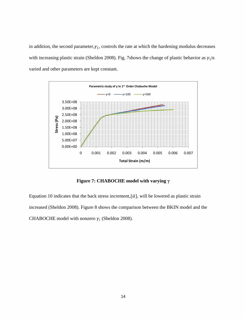
in addition, the second parameter,𝛾1, controls the rate at which the hardening modulus decreases

with increasing plastic strain (Sheldon 2008). Fig. 7shows the change of plastic behavior as 𝛾1is

varied and other parameters are kept constant.

Figure 7: CHABOCHE model with varying γ

Equation 10 indicates that the back stress increment,{𝛼 }, will be lowered as plastic strain

increased (Sheldon 2008). Figure 8 shows the comparison between the BKIN model and the

CHABOCHE model with nonzero 𝛾𝑖 (Sheldon 2008).

0.00E+00

5.00E+07

1.00E+08

1.50E+08

2.00E+08

2.50E+08

3.00E+08

3.50E+08

0 0.001 0.002 0.003 0.004 0.005 0.006 0.007

Stre

ss (

Pa)

Total Strain (m/m)

Parametric study of γ in 1st Order Chaboche Model

γ=0 γ=100 γ=500

15

Figure 8: BKIN model and CHABOCHE with nonzero γ

Notice that the initial slope of the two models are the same at yielding stress, then the slope of

CHABOCHE model decreases to zero as total strain goes to infinity.

This research will use the first order CHABOCHE model because of its simplicity in

calibrating the model constants. This research also uses most of the material properties in

previous researches to calibrate these constants. The yielding stress, σyield, and C1 at specific

temperature are found by using the historical data in BKIN model. Those parameters are the

same as the yielding stress and tangent modulus at specific temperature in BKIN model. The

values of 𝛾1are found by curve fitting the actual data using ANSYS. Also, the elastic modulus,

which is a function of temperature, will be used with the CHABOCHE model to simulate the

elastic behavior of the specimen. Due to the use of the CHABOCHE model and the equation of

16

elastic modulus, the specimen is expected to be hardened or softened when the temperature

decreased or increased, respectively. These effects can be observed in Fig. 9a & 9b which show

the material behaviors of a smooth specimen under various temperature ranges and similar

monotonic load condition.

17

(a)

(b)

Figure 9a & 9b: Stress- Strain Behaviors of 6 Temperature Profiles using CHABOCHE

Model

0.00E+00

2.00E+02

4.00E+02

6.00E+02

8.00E+02

1.00E+03

1.20E+03

1.40E+03

0.00E+00 5.00E+00 1.00E+01 1.50E+01 2.00E+01 2.50E+01

Tem

pe

ratu

re (K

)

Time (s)

Temperature Profiles of 6 Different Cases with Similar Loading Condition

Case 1 Case 2 Case 3 Case 4 Case 5 Case 6

Stre

ss (

MP

a)

Total Strain (m/m)

18

Considering case 1, 2, 4, and 5, the stress strain curve is lowest in case 5, where the temperature

is highest. This fact indicates that the material will undergo more deformation for the same stress

level. Case 2 always has the lowest temperature in comparison to 1, 4, and 5 so that its material

is the stiffest. As a result, case 2 has highest stress strain curve and lowest plastic strain. Case 1

and 4 are similar so their stress strain curves are expected to reassemble each other. In addition,

since the temperature in case 3 is linearly decreasing from 1273.15K to 473.15K and the

temperature in case 6 is constant at 473.15K, case 6 is supported to be stiffest. The stress strain

curve of case 6 is, therefore, higher than case 3. The conclusions derived from Figure 9a & 9b

confirm that the accuracy of the CHABOCHE used in this research.

2.4 Thermomechanical Fatigue

Thermomechanical fatigue (i.e. TMF) is the condition where the specimen undergoes cyclic

load and temperature. This condition reduces the lifespan of components in many high

temperature and pressure applications such as turbine blades. Due to the difficulty in simulating

the thermal stress cycling, many early works used isothermal fatigue tests at various

temperatures and loads to approximate TMF condition. Thus, these works did not capture the

damage micromechanisms under fluctuated temperature (Changan Cai, Peter K. Liaw, Mingliang

Ye, Jie Yu 1999). The fatigue failure can be divided into 2 categories: High-cycle fatigue (HCF)

and Low-cycle fatigue (LCF). HCF is associated with small load so that the fatigue life exceeds

104 cycles. LCF uses sufficiently large load that results in the fatigue life less than 10

4. Besides

the magnitude of the load, TMF can be differentiated by the phase between the temperature and

19

the applied load. This Thesis will consider two extreme cases which are in-phase and out-phase

case. The relation between temperature and applied load of those cases are illustrated in Figure

10a & 10b

Figure 10 a & 10b: Relationship between applied load and temperature in in-phase and

out-phase case

-2000

-1500

-1000

-500

0

500

1000

1500

2000

-800

-600

-400

-200

0

200

400

600

800

0 20 40 60 80 100 120 140

Tem

pe

ratu

re (

K)

Ap

plie

d L

oad

(M

pa)

Temperature and Applied Load Relationship in In-phase Case

Applied Load(MPa) Temperature (K)

-2000

-1500

-1000

-500

0

500

1000

1500

2000

-800

-600

-400

-200

0

200

400

600

800

0 20 40 60 80 100 120 140

Tem

pe

ratu

re (

K)

Ap

plie

d L

oad

(M

pa)

Temperature and Applied Load Relationship in Out-phase Case

Applied Load (MPa) Temperature (K)

20

In the in-phase case, the temperature and applied load will reach their highest values at the same

time, thus the phase angle will be 0o. On the other hand, the out-phase case will have the phase

angle of 180o because the highest stress will occur at the lowest temperature.

2.5 Hypotheses

Even though Neuber's rule is not applicable for TMF, the elastic modulus in equation 5 is

temperature dependent. Therefore, it is possible to find an equivalent temperature, T*, that can

improve the accuracy of Neuber's rule in non-isothermal condition. Rewrite equation 5 in terms

of elastic modulus as

𝐸 𝑇∗ =𝑘𝑡

2∗𝑆2

𝜎𝜖 (12)

By using parametric study, the equation of 𝜎𝜖 can be deduced; thus, equation 12 will yield T*.

The goal of this Thesis is to use BKIN model to approximate the material behavior at the notch

root; thus, BKIN model should intercept Neuber's hyperbola at the highest stress as in Fig. 11

21

Figure 11: BKIN model used to approximate the material behavior

Additionally, equation 12 can be rewritten to find the elastic solution as

𝜖 =𝑘𝑡𝑆

𝐸(𝑇∗) (13)

Since T* makes equation12 valid, it will be able to make the equation 13 valid as well. In other

word, T* can be used to calculate the equivalent elastic modulus and elastic strain of the material.

Neuber hyperbola can also be combined with BKIN model to get

𝜎𝜖 = 𝐸𝑒𝑙𝑎𝑠𝑡𝑖𝑐 𝑇 . 𝜖2 , 𝜖 ≤ 𝜖𝑦𝑖𝑒𝑙𝑑

𝜖 𝐸𝑡𝑎𝑛𝑔𝑒𝑛𝑡 𝜖 − 𝜖𝑦𝑖𝑒𝑙𝑑 + 𝜎𝑦𝑖𝑒𝑙𝑑 , 𝜖 ≥ 𝜖𝑦𝑖𝑒𝑙𝑑 (14)

22

𝜎𝑦𝑖𝑒𝑙𝑑 in equation 14 can be found by plotting yielding stress as function of temperature versus

applied stress as function of temperature. The intersection of those plots will indicate both

yielding stress and temperature at yielding.

Figure 12: Applied Pressure intercepts Yielding Stress at Yield Temperature

T* can be used to calculate tangent modulus in the right hand side of equation 13. The left hand

side of equation 14 contains both stress and strain. As a result, they needed to be decoupled, and

the plastic strain will be calculated separately.

23

3. Numerical Simulation

3.1 Specimen Design

Due to symmetry, only ¼ of the test specimen will be modeled using ANSYS software.

Simple V-notch structure has been used to simulate the stress strain responses of IN939 under

cycling load and temperature. Material modeling will be set up using single, solid, and 8-notch

elements with the thickness of 2mm. The parametric study on the mesh size was carried out to

determine the best mesh size for the simulation. The pressure on the top of the specimen and

temperature will linearly increase so that they meet at their maximum values in the in-phase

case; oppositely, the maximum pressure will occur with the minimum temperature in the out-

phase case. The stress and strain at the notch are expected to be at maximum values during the in

phase case and at minimum values during the out of phase case due to the hardening of material

under low temperature. Also, pressure and temperature are selected so that plastic deformation

only happens around the notch to mimic the real turbine’s blade. Fixed supports will be applied

on two sides of the specimen, and the load will be applied on specimen’s top in type of pressure

as seen in Fig. 14 below.

Figure 13 Specimen Constraints

x

y Data obtained at 2 points

24

The elasticity behavior of the model is controlled by a polynomial equation, which is obtained by

curve fitting stress strain response of the historical data. In order to improve the model’s

accuracy, the plastic behavior is modeled with a built-in CHABOCHE model. The stress at 2

different points on the specimen will be collected to verify the material properties and boundary

conditions. Figure 15 shows the distribution of the stress at the notch. Notice that there are two

opposite regions in the picture, one is the maximum stress region and one is the minimum stress

region.

Figure 14: Von-Mises stress distribution

3.2 Formula Development

According to Neuber's rule, the max stress can be written as

𝜎𝜖 = 𝑓(𝐾𝑡 , 𝑆,𝑇𝑚𝑎𝑥 ,𝑇𝑚𝑖𝑛 ,𝛷) (15)

25

In this equation, 𝛷 is the phase angle. It is 0o for the in-phase case and 180

o for the out-phase

case. During TMF, the elastic modulus of the material changes as the temperature fluctuated;

thus, Neuber’s hypothesis, 𝜎𝜖, also changes accordingly. By using ANSYS, the stress-strain

solutions at the notch can be determined. As a result, the right side of Neuber's rule can be

written as

𝐾𝑡𝑆 2

𝐸(𝑇∗)= 𝑓(𝐾𝑡 , 𝑆,𝑇𝑚𝑎𝑥 ,𝑇𝑚𝑖𝑛 ,𝛷) (16)

By knowing the equation of E as a function of temperature, equation (16) can be used to find the

equivalent temperature, T*. In order to confirm that the Nuber's hypothesis is a function of the

parameters in the right hand side of equation (16), Eureqa Formulize program will be used to

find the equations of Neuber's hypothesis as functions of the combinations of those parameters.

Then these equations will be used to calculate the Calculated σ*ε. These new data will be plotted

against the actual values from ANSYS as in Fig. 16. Since all data points of the combination of

Tmax, Tmin, S, Φ, and Kt are lying on the line with the slope of 1, the parametric study verifies that

Neuber's hypothesis is a function of these parameters.

26

Figure 15: Parametric study on the combination of parameters in the right hand side of

equation (12)

Therefore the equation of the Neuber's hypothesis is

σ𝜖𝑡𝑜𝑡𝑎𝑙 = 6.24 ∗ 105Kt + 3.41 ∗ 103Φ + 0.0178 ∗ S + 1.73Tmin Φ + 3.7 ∗ 10−6STmax − 3.95 ∗

106 − 2.51 ∗ 10−5SΦ − 2.26Tmax Φ (17)

Note that this equation does not work under elastic condition because all parametric study data

include both elastic and plastic strain. However, this equation can be extended to account for

elastic condition by adding more data into the parametric study. Equation 17 also good for

y = 0.996x + 4568.

0.00E+00

2.00E+05

4.00E+05

6.00E+05

8.00E+05

1.00E+06

1.20E+06

1.40E+06

1.60E+06

1.80E+06

2.00E+06

4.50E+05 6.50E+05 8.50E+05 1.05E+06 1.25E+06 1.45E+06 1.65E+06 1.85E+06 2.05E+06

An

alyt

ical

σ*ε

(P

a)

Numerical σ*ε (Pa)

Numerical σ*ε vs. Analytical σ*ε

Tmax/min Tmax/min,P Tmax/min,P,Φ Tmax/min,P,Φ,Kt

27

temperature from 473.15 K to 1273.15 K, applied load from 0MPa to 130MPa, kt from 2.8 to

4.2, and phase angel equal 0o or 180

o.

Based on equation (16) and (17), the equation for the equivalent temperature can be found as

𝑇∗ =

1766.3 − 1.12 ∗

4.19∗1019 +1.19∗1012𝑆+2.2∗107Φ−3.98Kt𝑆2+2.4∗108𝑆𝑇𝑚𝑎𝑥 −1.6∗109𝑆Φ+1.16∗1014𝑇𝑚𝑖𝑛 Φ−1.5∗1014𝑇𝑚𝑎𝑥 Φ−2.6∗1020

−(6.24∗1012𝐾𝑡+1.78∗105𝑆+3.41∗1010∗Φ+37STmax −251SΦ+1.73∗107Tmin Φ−2.26∗107∗Tmax Φ−3.9∗1013 (18)

This equivalent temperature then can be used to find the elastic modulus, tangent modulus, and

yielding stress of the studying material. Note that these materials properties are good only for the

notched region. However, the equation can be used to calculate the material properties of a

normal specimen if the value of Kt is set to 1.

Besides calculating T*, calculating the maximum stress at the notch is also necessary to

determine the material behavior at the notch. In order to accomplish this goal, the stress and

elastic/plastic strain in the left hand side of equation 15 has to be separated discuss in Chapter

2.5.

28

4. Results and Discussion

By applying equation 18 to calculate T* for some cases, it appears that the equivalent

temperatures are slightly higher than the average temperature in the in-phase case and close to

the minimum temperature in the out-phase case. Then, the equivalent temperatures will be used

to calculate the elastic modulus and the tangent modulus in order to approximate the material

behavior of the notched specimen. Figure 17a and 17b show the results of two cases that undergo

same loading, 0MPa to 100MPa, and temperature range, 673.15K to 1073.15K, except that the

upper one is in-phase and the lower one is out-xphase.

29

(a)

0

50

100

150

200

250

300

350

400

450

0.00E+00 5.00E-04 1.00E-03 1.50E-03 2.00E-03 2.50E-03 3.00E-03 3.50E-03 4.00E-03

Stre

ss (

MP

a)

Strain (m/m)

Stress Strain Curve for In-Phase Case

Numerical Result Analytical Result

Initial Slope

30

(b)

Figure 16a & 16b : Analytical stress-strain curve and ANSYS stress-strain curve for in-

phase and out-phase cases

In general, the T*s compensate for change in temperature in booth in-phase and out-phase

case. The black dot lines represent the initial slopes of the stress-strain curves. In order words,

the dot lines show the elastic behavior of the material in BKIN model without the correction of

T*. For the in-phase case, T

* compensates for the decrease in elastic modulus by staying close to

the maximum temperature. Therefore, the analytical and numerical results in the elastic region

are very close to each other. In the out-phase case, T* stays close to the minimum temperature.

Thus, it keeps the analytical result from deviating from the numerical results. The stress strain

curve in the in-phase case, Fig.17a, also shows that the T* has decreased the slope of the elastic

0

50

100

150

200

250

300

350

400

450

0 0.0005 0.001 0.0015 0.002 0.0025 0.003

Stre

ss (

Mp

a)

Strain (m/m)

Stress Strain Curve for Out-Phase Case

Numerical Result Analytical Result

Initial Slope

31

curve. This fact increases the total strain of the specimen. The opposite happens to the out-phase

case, causing the total strain to decrease.

32

5. Conclusions

In conclusion, a formula to approximate T* and a method to calculate the stress strain

respond at the V-notch’s tip have been developed. T*

can be used in BKIN model to estimate

both the elastic and plastic modulus for IN939 notched specimen. The results suggest that T* is

able to compensate for the inaccurate caused by temperature’s changing in BKIN model. In

addition, the method works with other material and notch type given that different parametric

study is carried out for each specific case. Material behavior behind the notch’s tip can also be

calculated by employing other method such as Xu-Thompson-Topper’s formula which requires

the stress strain solution at the notch’s tip. This research’s result will give engineer the ability to

quickly approximate the material behavior at the notch’s tip on the gas turbine’s blade without

the use of FEA program.

33

6. Future Work

Equation 16 was developed with assumption that plastic deformation occurs at the notch

root; thus it is not applicable if the notch undergo elastic deformation. The future plan is to

increase number of data in the parametric study of Neuber’s rule so that it can account for cases

where the material undergoes only elastic deformation. In addition, future simulation can be

carried out with higher order for CHABOCHE model to closely simulate service conditions.

Besides improving the accuracy of the model, future simulations are also planned to evaluate the

quality of Etangent(T*).

34

Appendix

35

Appendix

ANSYS code

Finish

/Clear

/PREP7

!*****************************************************************************

**

!---Input parameters:

Finish

/PREP7

!---Geometric:

RAD_NTCH=.037*0.0254 ! Root radius of notch [m]

ANG_NTCH=60 ! Angle of notch

[deg]

DIA_NTCH=.251*0.0254 ! Diameter of specimen at notch [m]

DIA_RED=.360*0.0254 ! Reduced diameter of specimen [m]

RAD_SHLD=1.0*0.0254 ! Radius of reduction shoulder [m]

DIA_GRIP=.5*0.0254 ! Diameter of specimen grip [m]

LEN_GRIP=1.25*0.0254 ! Lenght of specimen grip [m]

LEN_BAR=4*0.0254 ! Total length of specimen [m]

!*****************************************************************************

**

!---Parameters derived from geometric relationships

*AFUN, DEG

l1=LEN_BAR/2

l2=LEN_GRIP

d1=DIA_GRIP/2

d2=DIA_RED/2

r1=RAD_SHLD

r2=RAD_NTCH

t=DIA_NTCH/2

a=ANG_NTCH/2

x1=d2+r1-d1

y1=sqrt((r1*r1)-(x1*x1))

x2=sin(a)*r2

y2=cos(a)*r2

x3=(y2/tan(a))-(r2-x2)-t

y3=tan(a)*(d2+x3)

36

!*****************************************************************************

**

!---Specimen Geometry:

!---Keypoints

k, 1, 0.0, 0.0

k, 2, 0.0, l1

k, 3, d1, l1

k, 4, d1, l1-l2

k, 5, d2, l1-l2-y1

k, 6, d2+r1, l1-l2-y1

k, 7, d2, y3

k, 8, t+r2-x2, y2

k, 9, t, 0.0

k, 10, t+r2, 0.0

! Lines

L, 1, 2 ! Line 1

L, 2, 3 ! Line 2

L, 3, 4 ! Line 3

Larc, 4, 5, 6, r1 ! Line 4

L, 5, 7 ! Line 5

L, 7, 8 ! Line 6

Larc, 8, 9, 10, r2 ! Line 7

L, 9, 1 ! Line 8

! Areas

AL, all

ksel,all

!*****************************************************************************

**

!---Element Type and Material Number

ET,1,PLANE183,,,3

R,1,0.002

MAT,1

!*****************************************************************************

**

!---Define Properties of Material 1

!---Elastic Properties

MPTEMP,1,293.15,573.15,773.15,1073.15,1173.15,1223.15

37

MPDATA,EX,1,1,2.117e11,1.941e11,1.808e11, 1.578e11,1.49e11,1.442e11

MPDATA,PRXY,1,1,0.36976264,0.41036665,0.4428308,0.48523527,0.49529229,0.49921871

MPDATA,DENS,1,1,8.36576e9,8.27988e9,8.221e9,8.13653e9,8.1094e9,8.09603e9

!

!---CHABOCHE Properties

TB,CHABOCHE,1,10,1 !Activate CHABOCHE data table

!

TBTEMP,293.15

TBDATA,1,3.51e8,100000e6,100 !TBDATA,mat,Yeild Stress, C1,G1

!

TBTEMP,373.15


!

TBTEMP,573.15


!

TBTEMP,738.15


!

TBTEMP,773.15


!

TBTEMP,973.15


!

TBTEMP,1073.15


!

TBTEMP,1123.15


!

TBTEMP,1173.15


!

TBTEMP,1223.15


!*****************************************************************************

!---Mesh Area

! Mesh Area

AMESH,ALL,,, ! Mesh the Speciment

38

!---Refine the mesh

AREFINE,1,,,3,1,OFF,ON ! Refine Mesh for the area

!NREFINE,70,,,4,1

FINISH

!!****************************************************************************

*****

!Machanical Cycling Parameter

load_ini=1000 !1000

load_fin=1300 !1500

load_inc=100.0

tempMAX_ini=473.15 !473.15

tempMAX_fin=1273.15 !1073.15

tempMAX_inc=100.0

tempMIN_ini=673.15 !673.15

tempMIN_fin=473.15 !473.15

tempMIN_inc=-100.0

*DO,load,load_ini,load_fin,load_inc ! Changing load_max [N]

*DO,temp_max,tempMAX_ini,tempMAX_fin,tempMAX_inc ! Changing temp max [K]

*DO,temp_min,tempMIN_ini,tempMIN_fin,tempMIN_inc ! Changing them min [K]

!Solution

/Solution

!Specify the analysis type

ANTYPE,TRANS,,2,1,,

TRNOPT,FULL,,,,,

nropt,auto ! Uses Newton-Raphson

lnsrch,auto ! Auto line searching for NR

!*****************************************************************************

! Constraint

DL,8,1,UY,0,1 !Line8: Zero

Displacement in x,y direction

DL,1,1,UX,0,1 !Line1: Zero

Displacement in x,y direction

loadmax=load/0.0000128 !Max Load [N]

loadmin=-load/0.0000128 !Min Load [N]

frq_load=0.25

39

numcyc=10

SubStep=10

T_load=1/frq_load

!****************************************************************************

BFUNIF,TEMP, temp_min !Initial Temperature

*DO,i,0,numcyc,1

SFL,2,PRES,-loadmax

BFA,1,TEMP,temp_max

KBC,0

TIME,(T_load*(1/4)+i*T_load)*10 !Time at the end of this load step

NSUBST,SubStep,,,OFF

LSWRITE,i

OUTRES,ALL,ALL

Solve

SFL,2,PRES,-loadmin

BFA,1,TEMP,temp_min

KBC,0

TIME,(T_load*(3/4)+i*T_load)*10 !Time at the end of this loadtep

NSUBST,SubStep,,,OFF

LSWRITE,i+1

OUTRES,ALL,All

Solve

*ENDDO

OUTRES,ALL,All !Output ALL

properties for ESOL

FINISH

!*****************************************************************************

!Post Solution

/POST26

/NUMVAR,1000

/FORMAT,,E !Set up

Decimal notation

/FORMAT,,,17,9 !Setup sace

vetween values

/OUTPUT,C:\notch\Notch_Kt=_%load%_%-load%_%temp_max%_%temp_min%,txt

ESOL,2,36,68,EPEL,Y

ESOL,3,36,68,EPPL,Y

ESOL,4,36,68,S,Y

40

ESOL,5,205,949,BFE,TEMP

ESOL,6,30,259,S,Y

PRVAR,2,3,4,5,6

*ENDDO

*ENDDO

*ENDDO

FINISH

41

References

Albeirutty H. M.; Alghamdi S. A.; Najjar S. Y. "Heat Transfer analysis for a Multistage Gas Turbine Using

Different Blade-Cooling Schemes." Applied Thermal Engineering 24 (2004): 563-577.

ANSYS. ANSYS Commands Reference. ANSYS Inc, 2011.

Changan Cai, Peter K. Liaw, Mingliang Ye, Jie Yu. "Recent Developments in the Thermomechanical

Fatigue Life Prediction of Superalloys." JOM-e 51 (1999).

Delargy, K. M.; Shaw S. W. K.; Smith G. D. W. "Effects of Heat treatment on Mechanical Properties of

High-Chromium Nickel-Base Superallow IN939." Materials Science & Technology 2 (1986): 1031-1037.

Dowling, N. "Notched Member Fatigue Life Predictions Combining Crack Initiation and Propagation."

Fatigue of Engineering Materials and Structures 2 (1979): 129-138.

Doyle, John. Simulating of Ratchetting and Shakedown. 11 8, 2011.

E., Inglis C. "Stresses in a Plate Due to the Presence of Cracks and Sharp Corners." Trans. Inst. Naval

Architects, 1913: 219-230.

Filippini; Mauro. "Stress Gradient Calculations at Notches." Int J Fatigue 22 (2000): 397-409.

Gordon Ali P.; Eric P. Williams; Michael Schulist. "Applicability of Neuber's Rule for Thermomechanical

Fatigue." ASME Conf. Proc, 2008.

Jovanovic M. T.; Miskovic Z.; Lukic B. "Microstructure and Stress-Rupture life of Polycrystal, Directionally

Solidified and Signle Crystal Castings of Nickel-Based IN939." Materials Characterization 40 (1998): 261-

268.

Miskovic Z.; Janovic M.; Gligic M.; Likic B. "Microstructural Investigation of IN939 Supperalloy." Cacuum

43: 709-711.

Monlinski K.; Glinka G. "A Method of Elastic-Plastic Stress and Strain Calculation at a Notch Root."

Materials Science and Engineering 50: 93-100.

Mutter, Nathan J. "Stress Concentration Factors for V-Notched Plates under Axisymmetric Pressure."

UCF's Mechanics of Materials Research Group . 2010. http://momrg.cecs.ucf.edu/theses.php (accessed 3

5, 2013).

Nazmy M. Y.; Wuthrich C. "Creep Crack Growth in IN738 and IN939 Nickel-Base Superalloys." Materials

Science and Engineering 61 (1983): 119-125.

42

Neuber, H. "Theory of Stress Concentration for Shear-Strained Prismatical Bodies with Arbitrary Non-

linear Stress-Strain Law." Journal of Applied Mechancis 27 (1961): 544-551.

Ramberg W.; Osgood W. R. "Description of Stress-Strain Curves by Three Paramenters." National

Advisory Committee for Aeronautics, 1943.

Sheldon, Imaoka. "Chaboche Nonlinear Kinematic Hardening Model." ANSYS Release: 12.0.0 (ANSYS),

2008.

Xu R. X.; Thompson J. C.; Topper T. H. "Practical Stress Expressions for Stress Concentration of Notches."

Fatigue Fracture Engineering Material Structure 18 (7/8) (1995): 885-895.

application of non-local approaches for …momrg.cecs.ucf.edu/theses/nguyent_him.pdf · methods...

Documents