application of optimization of compressors used in air

Purdue UniversityPurdue e-PubsInternational Refrigeration and Air ConditioningConference School of Mechanical Engineering

2018

Application of Optimization of Compressors usedin Air conditioning unitsJoel Vinod AralikattiBradley University, United States of America, [email protected]

David ZietlowBradley University, United States of America, [email protected]

Follow this and additional works at: https://docs.lib.purdue.edu/iracc

This document has been made available through Purdue e-Pubs, a service of the Purdue University Libraries. Please contact [email protected] foradditional information.Complete proceedings may be acquired in print and on CD-ROM directly from the Ray W. Herrick Laboratories at https://engineering.purdue.edu/Herrick/Events/orderlit.html

Aralikatti, Joel Vinod and Zietlow, David, "Application of Optimization of Compressors used in Air conditioning units" (2018).International Refrigeration and Air Conditioning Conference. Paper 2018.https://docs.lib.purdue.edu/iracc/2018

https://docs.lib.purdue.edu?utm_source=docs.lib.purdue.edu%2Firacc%2F2018&utm_medium=PDF&utm_campaign=PDFCoverPages

https://docs.lib.purdue.edu/iracc?utm_source=docs.lib.purdue.edu%2Firacc%2F2018&utm_medium=PDF&utm_campaign=PDFCoverPages


https://docs.lib.purdue.edu/me?utm_source=docs.lib.purdue.edu%2Firacc%2F2018&utm_medium=PDF&utm_campaign=PDFCoverPages


https://engineering.purdue.edu/Herrick/Events/orderlit.html

https://engineering.purdue.edu/Herrick/Events/orderlit.html

2563, Page 1

17th International Refrigeration and Air Conditioning Conference at Purdue, July 9-12, 2018

Application of Optimization Study of Compressors Used in Air Conditioning

Systems

Joel V ARALIKATTI* 1, Dr. David C ZIETLOW 2

1Graduate Student, Department of Mechanical Engineering, Bradley University,

Peoria, Illinois, USA

[email protected]

2 Professor, Department of Mechanical Engineering, Bradley University,

Peoria, Illinois, USA

[email protected]

* Joel V ARALIKATTI

ABSTRACT

Total life-cycle cost of a system refers to the costs incurred by the owner over the entire life of the system. The two

main components of this are: 1) initial cost: cost to purchase the system, often defined by the total/maximum

capacity and quality of the system, and 2) operating cost: the cost of operation over the entire life of the system,

defined by the daily usage and the efficiencies of the system and its components. Most compressors are designed

with a focus on minimizing the initial cost. Minimal data are available on the selection of a compressor based on its

design variables and the corresponding cost impact. A comprehensive link between the design requirements and

their initial and operating cost implications is lacking in the industry. This project addresses this issue by analyzing

the impact of design variables on the total life cycle cost of an automobile air conditioning (AC) unit when located

in different climatic zones. Using an earlier, experimentally validated, analytical model, the isentropic efficiency and

volumetric efficiency of a reciprocating compressor are varied to suit the environmental conditions of four

climatically diverse cities (with respect to the temperature, average length of cooling season and humidity) i.e.

Phoenix, AZ, Peoria, IL, Minneapolis, MN and Miami, FL. The model connects the efficiencies to primary design

variables of a compressor, namely the polytrophic exponent, clearance ratio, geometry, etc. The lowest possible life-

cycle cost and the corresponding compressor specifications are determined and reported. Using this in the design of

AC units (residential/commercial, automobile) will result in the best compressor design for a given application. For

colder climates (Peoria and Minneapolis) the optimum isentropic efficiency and volumetric efficiency of a

compressor averaged over the cooling season at 51% and 69% respectively, whereas for hotter climates (Phoenix

and Miami) the efficiencies averaged at 60% and 73% respectively.

1. INTRODUCTION

Total life cycle costs provide a realistic optimum which can be used to justify a particular compressor design. Other

objective functions such as efficiency do not yield realistic optimums. Total life-cycle cost of a system is defined as

the total cost incurred by the owner throughout the life of the system including planning, design, acquisition,

support, operating costs and any other costs directly attributable to owning or using the asset. It involves two main

components: i) Initial Cost (IC): cost to purchase the system, often defined by the total/maximum capacity and the

quality of the system. ii) Operating Cost (OC): the cost of operation over the entire life of the system, defined by the

daily usage and the efficiencies of the system and its components.

1.1 Assumptions The following assumptions were made for the present study -

• The analytical model is largely restricted to a reciprocating type compressor

• It considers only a simple model of the condenser and evaporator

• Valve leakage is restricted to reed valves used in reciprocating compressors

• A steady state flow of refrigerant and air (changes in kinetic and potential energies through each component

considered negligible)

2563, Page 2


2. ANALYTICAL MODEL

One of the first steps in the project was to create an analytical model of an AC unit that runs on a reciprocating type

compressor. Taking minimum total cost of the system as the objective function, equations are derived to link the

design variables of the compressor to the initial and operating costs of the system. Initial cost is defined as a function

of the work input, isentropic efficiency and the volumetric efficiency of the compressor. Considering the scope of

this project, costs were assumed to depend only on the compressor characteristics. Two intermediate design

variables were considered in this project: 1) isentropic efficiency 2) volumetric efficiency. These intermediate

design variables are further linked to the primary design parameters of a compressor like the pressure ratio, valve

geometry (surface roughness, parallelism and flatness of the valve and valve seating area), clearance ratio, and the

frictional losses between cylinder wall and the piston. Using conservation of energy around the components of the

AC unit, equations are derived linking the work of the compressor to the heat transfer rate at the condenser and the

evaporator. The condenser and the evaporator heat exchangers are modeled using effectiveness NTU relations.

Maximum heat transfer rate equations link the air-side and the refrigerant-side of the heat exchangers.

The operating cost of the AC unit was taken as a function of the compressor work input. The tradeoff here was that

the operating cost of the AC unit decreases if the isentropic and volumetric efficiencies of the compressor are high.

However, a higher efficiency compressor also incurs a larger initial cost. Thus, the compressor efficiencies must be

optimized for a given application and working environment.

To validate the analytical model an experimental AC apparatus was used to produce data and compare to the results

from the analytical model. The experimental apparatus has the capability to vary the compressor speed by varying

the electric frequency of the drive. The compressor speed was varied up to 2000 rpm with a resolution of 1 rpm. The

mass flow rate and temperature of the air over the condenser was controlled using dampers on the inlet of the

condenser air duct and the return air duct. The damper position varied on a scale of 0 to 90 degrees. Velocity of air

over different damper openings were recorded to arrive at the volumetric flow rate through condenser. The mass

flow rate of air over the evaporator was controlled by controlling the fan speed. The fan speed was varied over 6

different speeds. By measuring the velocity of the air, the volumetric flow rate of air was determined.

For this project, the compressor speed, flow rate over condenser and evaporator are stratified into 3 levels: low,

medium, and high. For the compressor speed, the respective levels are 1000, 1500, and 2000 rpm. For the condenser,

the respective damper openings refer to 60deg, 45deg, and 90deg opening of the damper. For the evaporator, the

respective fan speeds refer to 4, 5, and 6 on the scale. Permutating these three parameters yield 27 different

combinations of settings. The AC unit was run for each of these settings till the AC unit achieved a steady state.

Steady state was verified by taking temperature and pressure readings every five minutes. It was observed that after

15 minutes, the AC unit achieved a steady state. Once the steady state was reached, all the instrument readings were

taken every five minutes for five repetitions. The data was averaged over the five readings to get the final set of data

for that setting. This cycle was repeated for all the 27 sets of operating conditions.

2.1 Optimization The experimental data was then used to validate the empirical parameters, such as the multipliers in the Nusselt

correlations, used in the analytical model. Validation was based on the root mean square (RMS) error computed

between the compressor power calculated from the model and the actual compressor power input. The compressor

work in the model was computed using the equations for isentropic efficiency and volumetric efficiency and the

primary design variables. The compressor power was compared for all the 27 different settings. The min/max

feature in Engineering Equation Solver (EES) was used to minimize the RMS error as a function of the primary

design variables: coefficient of isentropic efficiency (CC_eta), polytropic exponent of the compression cycle

(gamma), clearance ratio of the cylinder (clear_ratio), coefficient of volumetric efficiency (C_gam), the pressure

drop due to refrigerant mass left in the clearance volume (pressure_drop) and the discharge coefficient for the

leakage flow rate through the valves (discharge_c). The optimum values for these primary design variables are

determined from the validated model. The optimum primary design variables are then used in the analytical system

model to compute the total cost of the AC unit.

2563, Page 3


Figure 1: The variation of isentropic and volumetric efficiencies with the primary design variables of the

system are as shown. The optimum values, based on minimum RMS error, for each design variable is

identified on each plot.

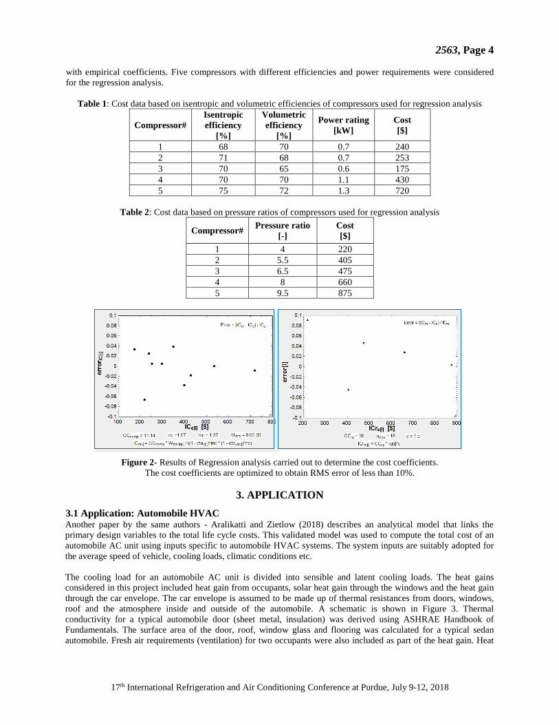
2.2 Cost Data Cost coefficients are the empirical coefficients required to calculate the initial cost of the compressor based on the

power rating, efficiencies and the pressure ratio.

Cost coefficients CCcomp and CCrp are obtained using regression analysis.

Obtaining cost data was one of the challenging tasks of this project, as there is not much cost data available based on

the primary design variables of compressors. Cost data was obtained from supplier websites based on the isentropic,

volumetric efficiencies, and pressure ratio of the compressor. Using regression analysis, an equation was derived

2563, Page 4


with empirical coefficients. Five compressors with different efficiencies and power requirements were considered

for the regression analysis.

Table 1: Cost data based on isentropic and volumetric efficiencies of compressors used for regression analysis

Compressor#

Isentropic

efficiency

[%]

Volumetric

efficiency

[%]

Power rating

[kW]

Cost

[$]

1 68 70 0.7 240

2 71 68 0.7 253

3 70 65 0.6 175

4 70 70 1.1 430

5 75 72 1.3 720

Table 2: Cost data based on pressure ratios of compressors used for regression analysis

Compressor# Pressure ratio

[-]

Cost

[$]

1 4 220

2 5.5 405

3 6.5 475

4 8 660

5 9.5 875

Figure 2- Results of Regression analysis carried out to determine the cost coefficients.

The cost coefficients are optimized to obtain RMS error of less than 10%.

3. APPLICATION

3.1 Application: Automobile HVAC Another paper by the same authors - Aralikatti and Zietlow (2018) describes an analytical model that links the

primary design variables to the total life cycle costs. This validated model was used to compute the total cost of an

automobile AC unit using inputs specific to automobile HVAC systems. The system inputs are suitably adopted for

the average speed of vehicle, cooling loads, climatic conditions etc.

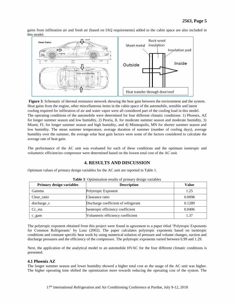
The cooling load for an automobile AC unit is divided into sensible and latent cooling loads. The heat gains

considered in this project included heat gain from occupants, solar heat gain through the windows and the heat gain

through the car envelope. The car envelope is assumed to be made up of thermal resistances from doors, windows,

roof and the atmosphere inside and outside of the automobile. A schematic is shown in Figure 3. Thermal

conductivity for a typical automobile door (sheet metal, insulation) was derived using ASHRAE Handbook of

Fundamentals. The surface area of the door, roof, window glass and flooring was calculated for a typical sedan

automobile. Fresh air requirements (ventilation) for two occupants were also included as part of the heat gain. Heat

2563, Page 5


gains from infiltration air and fresh air (based on IAQ requirements) added to the cabin space are also included in

this model.

Figure 3: Schematic of thermal resistance network showing the heat gain between the environment and the system.

Heat gains from the engine, other miscellaneous items in the cabin space of the automobile, sensible and latent

cooling required for infiltration of air and water vapor were all considered part of the cooling load in this model.

The operating conditions of the automobile were determined for four different climatic conditions: 1) Phoenix, AZ

for longer summer season and low humidity, 2) Peoria, IL for moderate summer season and moderate humidity, 3)

Miami, FL for longer summer season and high humidity, and 4) Minneapolis, MN for shorter summer season and

low humidity. The mean summer temperature, average duration of summer (number of cooling days), average

humidity over the summer, the average solar heat gain factors were some of the factors considered to calculate the

average rate of heat gain.

The performance of the AC unit was evaluated for each of these conditions and the optimum isentropic and

volumetric efficiencies compressor were determined based on the lowest total cost of the AC unit.

4. RESULTS AND DISCUSSION

Optimum values of primary design variables for the AC unit are reported in Table 1.

Table 3: Optimization results of primary design variables

Primary design variables Description Value

Gamma Polytropic Exponent 1.25

Clear_ratio Clearance ratio 0.0098

discharge_c Discharge coefficient of refrigerant 0.1289

Cc_eta Isentropic efficiency coefficient 0.0406

c_gam Volumetric efficiency coefficient 1.37

The polytropic exponent obtained from this project were found in agreement to a paper titled ‘Polytropic Exponents

for Common Refrigerants’ by Lenz (2002). The paper calculates polytropic exponents based on isentropic

conditions and constant specific heat work by using numerical solution of pressure and volume changes, suction and

discharge pressures and the efficiency of the compressor. The polytropic exponents varied between 0.99 and 1.29.

Next, the application of the analytical model to an automobile HVAC for the four different climatic conditions is

presented.

4.1 Phoenix AZ The longer summer season and lower humidity showed a higher total cost as the usage of the AC unit was higher.

The higher operating time shifted the optimization more towards reducing the operating cost of the system. The

Heat transfer through door/roof

2563, Page 6


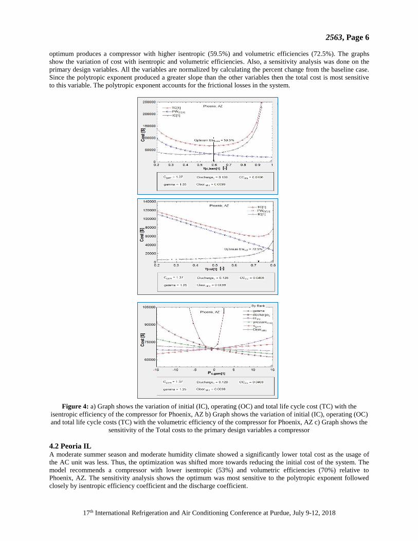
optimum produces a compressor with higher isentropic (59.5%) and volumetric efficiencies (72.5%). The graphs

show the variation of cost with isentropic and volumetric efficiencies. Also, a sensitivity analysis was done on the

primary design variables. All the variables are normalized by calculating the percent change from the baseline case.

Since the polytropic exponent produced a greater slope than the other variables then the total cost is most sensitive

to this variable. The polytropic exponent accounts for the frictional losses in the system.

Figure 4: a) Graph shows the variation of initial (IC), operating (OC) and total life cycle cost (TC) with the

isentropic efficiency of the compressor for Phoenix, AZ b) Graph shows the variation of initial (IC), operating (OC)

and total life cycle costs (TC) with the volumetric efficiency of the compressor for Phoenix, AZ c) Graph shows the

sensitivity of the Total costs to the primary design variables a compressor

4.2 Peoria IL A moderate summer season and moderate humidity climate showed a significantly lower total cost as the usage of

the AC unit was less. Thus, the optimization was shifted more towards reducing the initial cost of the system. The

model recommends a compressor with lower isentropic (53%) and volumetric efficiencies (70%) relative to

Phoenix, AZ. The sensitivity analysis shows the optimum was most sensitive to the polytropic exponent followed

closely by isentropic efficiency coefficient and the discharge coefficient.

2563, Page 7



isentropic efficiency of the compressor for Peoria, IL b) Graph shows the variation of initial (IC), operating (OC)

and total life cycle costs (TC) with the volumetric efficiency of the compressor for Peoria, IL c) Graph shows the


4.3 Minneapolis, MN Characterized by a short summer season and moderately humid climate generated a lower total cost. The usage of

the AC unit was the least among other cities considered, thus the optimization was shifted more towards reducing

the initial cost of the system. Thus, a less expensive compressor with a corresponding lower isentropic (49.5%) and

volumetric efficiencies (67.5%) produced the minimum total cost. The graphs show the variation of cost with

isentropic and volumetric efficiencies and also a sensitivity analysis of the total costs to the primary design

parameters.

2563, Page 8



isentropic efficiency of the compressor for Minneapolis, MN b) Graph shows the variation of initial (IC), operating

(OC) and total life cycle costs (TC) with the volumetric efficiency of the compressor for Minneapolis, MN c) Graph

shows the sensitivity of the Total costs to the primary design variables a compressor

4.4 Miami, FL Characterized by a longer summer season and high humidity climate, the air conditioning system showed a

significantly higher total cost as the usage of the AC unit was high. Thus, the optimization was shifted more towards

reducing the operating cost of the system. Therefore, a more expensive compressor with higher isentropic (59.5%)

and volumetric efficiencies (72.5%) could be justified.

2563, Page 9



isentropic efficiency of the compressor for Miami, FL b) Graph shows the variation of initial (IC), operating (OC)

and total life cycle costs (TC) with the volumetric efficiency of the compressor for Miami, FL c) Graph shows the


5. CONCLUSION

The project successfully established the relation between the design variables of an air conditioning compressor and

its total life cycle cost. The model details a logical progression of equations linking the primary design parameters to

the objective function (minimizing total cost). The experimentally validated model was applied to an automobile AC

to understand how the compressor optimization varied with operating conditions. The model is used to determine the

best compressor for a given application which would yield the minimum total life cycle cost. For illustration, four

different climate conditions, covering a wide range, were studied and the results discussed. A summary of the same

is provided in the table below. The table also lists the latent and sensible cooling loads and the resulting optimum

compressor efficiencies.

2563, Page 10


Table 4: Summary of model predictions for different climate conditions

City Climate Sensible load

[kW]

Latent load

[kW]

CDD

[oC-days]

Optimum values

based on minimum

total life cycle costs

Eta_isen Eta_vol

Phoenix, AZ High temp, low humidity 4.395 3.322 5207 59.5 72.5

Peoria, IL Moderate temp, moderate

humidity 2.568 0.287 1360 53 70

Minneapolis, MN Low temp, moderate

humidity 2.15 0.833 1036 49.5 67.5

Miami, FL High temp, high humidity 3.763 1.345 4684 59.5 72.5

NOMENCLATURE

AC Air Conditioning

AZ Arizona

IL Illinois

MN Minnesota

FL Florida

IC Initial Cost

OC Operating Cost

NTU Number of Transfer Units

RPM Rotations Per Minute

RMS Root Mean Square

CCcomp Cost coefficient for power rating

W_dot_in Power rating of the compressor (rate of work input)

Eta_c_isen Isentropic efficiency

Eta_vol Volumetric efficiency

CCrp Cost coefficient for pressure ratio

rp Pressure ratio

EES Engineering Equation Solver

CC_eta Coefficient of isentropic efficiency

Gamma Polytropic exponent

Clear_ratio Clearance ratio of the cylinder

C_gam Coefficient of volumetric efficiency

Discharge_c Discharge coefficient for the leakage flow rate through the valves

HVAC Heating, Ventilating and Air-Conditioning

ASHRAE American Society of Heating, Refrigerating and Air-conditioning Engineers

TC Total life cycle Cost

REFERENCES Handbook of ASHRAE - Fundamentals (2013). American Society of Heating Refrigerating and Air Conditioning

Engineers.

Thermodynamics (2010). International Compressor Engineering Conference. Paper 2004. Zietlow, David C.,

Optimization of Cooling Systems (2016). Momentum Press Thermal Science and Energy Engineering Collection

Aralikatti, J, Zietlow, D (2018). Optimization of Compressors used in Air Conditioning Systems

application of optimization of compressors used in air

Documents