arab academy for science, technology and maritime … · students contribution “optimization of...
TRANSCRIPT
Arab Academy for Science, Technology and Maritime
Transport
College of Engineering and Technology
Department of Industrial and Management Engineering
B. Sc. Final Year Project
Optimization of Traffic Signal Timings
Using Genetic Algorithm, Simulation, and FPGA control
Presented By:
Ahmed Aziz Ezzat Julia El Zoghby
Mohamed El Ahmar Nermine Hany
Azmy Mehelba Ezz Abou Emira
Supervised By:
Prof. Ahmed F. Abdel Moniem
Prof. Khaled S. El-Kilany
Dr. Hala A. Farouk
J U L Y – 2 0 1 3

DECLARATION
I hereby certify that this report, which I now submit for assessment on the programme
of study leading to the award of Bachelor of Science in Industrial and Management
Engineering, is all my own work and contains no Plagiarism. By submitting this report,
I agree to the following terms:
Any text, diagrams or other material copied from other sources (including, but not
limited to, books, journals, and the internet) have been clearly acknowledged and
cited followed by the reference number used; either in the text or in a
footnote/endnote. The details of the used references that are listed at the end of
the report are confirming to the referencing style dictated by the final year project
template and are, to my knowledge, accurate and complete.
I have read the sections on referencing and plagiarism in the final year project template.
I understand that plagiarism can lead to a reduced or fail grade, in serious cases, for the
Graduation Project course.
Student Name: Ahmed Aziz Ezzat
Registration Number: 08102254
Signed: ________________________
Date: 23 – 06 – 2013
Student Name: Julia El Zoghby
Registration Number: 08100357
Signed: ________________________
Date: 23 – 06 – 2013
Student Name: Nermine Hany
Registration Number: 08102042
Signed: ________________________
Date: 23 – 06 – 2013
Student Name: Mohamed El Ahmar
Registration Number: 08101591
Signed: ________________________
Date: 23 – 06 – 2013
Student Name: Ezz Abou Emira
Registration Number: 08100714
Signed: ________________________
Date: 23 – 06 – 2013
Student Name: Azmy Mehelba
Registration Number: 08102567
Signed: ________________________
Date: 23 – 06 – 2013

STUDENTS CONTRIBUTION
“Optimization of Traffic Signal Timings Using Genetic Algorithm, Simulation and
FPGA Control”
By:
Ahmed Aziz Ezzat
Julia El Zoghby
Nermine Hany
Mohamed El Ahmar
Ezz Abou Emira
Azmy Mehelba
Chapter Title Contributors
1 Introduction All students
2 Literature Review All students
3 Data Collection and Statistical Analysis Julia El Zoghby
Nermine Hany
Mohamed El Ahmar
Ahmed Aziz Ezzat
Ezz Abou Emira
4 Analytical Modeling and Genetic Algorithm Ahmed Aziz Ezzat
5 Simulation and Modeling of Actual system Julia El Zoghby
Nermine Hany
Mohamed El Ahmar
Ahmed Aziz Ezzat
6 Simulation of proposed scenario1 and 3D animation Mohamed El Ahmar
7 Simulation of an adaptive traffic control system Nermine Hany
8 Optimization using simulation approach Julia El Zoghby
9 Hardware in Traffic control Ezz Abou Emira
10 FPGA control in a pre-timed traffic system Ahmed Aziz Ezzat
11 FPGA control in an adaptive traffic system Azmy Mehelba
12 Conclusions and Recommendations All students

ACKNOWLEDGMENT
We have taken efforts in this project. However, it would have been impossible without
the kind support and help of our organization.
We would like to express our sincere appreciation and deepest gratitude to Prof. Ahmed
F. Abdel Moniem. This work could not have been completed without his valuable
guidance and immense knowledge.
A special acknowledgement belongs to our dearest professor Khaled S. El-Kilany for
his active cooperation and support during the period of this project. We deeply
appreciate how he invests his full effort in guiding us and enlightening our way.
We are also indebted to Dr. Hala A. Farouk for her support during the preparation of
this work. We have learned a lot and benefited a great deal by her critical comments and
suggestions.
Finally, we would like to thank our families and friends for their encouragement and
support throughout our lives.

ABSTRACT
Traffic congestion is a major problem in vastly populated cities. This project focuses on
the traffic crisis seen in Alexandria, which occurs due to the absence of a reliable
control strategy that regulates the traffic signal lights. As a result, a substantial growth
of the vehicles’ queue lengths and delays emerges. The main aim of this project is to
minimize the traffic congestion for a traffic control system, considering the traffic signal
timings rendered to a number of control points in specified intersections. In order to
satisfy this goal, a set of objectives to be carried out through the project are established.
The main objectives include developing an analytical model representing the traffic
system and proposing a solution approach using the Genetic Algorithm technique.
Furthermore, developing a simulation model for the problem in order to replicate and
analyse the performance of the real system, as well as suggesting better scenarios to
improve the overall system efficiency. Furthermore, a simulation model is developed to
represent a smart traffic control system, and evaluate its correspondent performance
compared to the current situation. In addition, employing optimization using simulation
methodology to reach the best possible traffic light timings, and last but not least,
studying the possibility of applying FPGA’s for the control of traffic systems.
The report focuses on generating different scenarios and various solutions through
experimenting with the developed models in order to optimize the traffic signal timings.
Comparisons are held between different approaches and methodologies to achieve the
best possible performance and cut off the traffic congestion problem from its root
causes.

i
TABLE OF CONTENTS
LIST OF FIGURES ......................................................................................................V
LIST OF TABLES...................................................................................................... IX
LIST OF ACRONYMS/ABBREVIATIONS ............................................................ XI
LIST OF SYMBOLS ................................................................................................ XII
1 INTRODUCTION ................................................................................................. 1
1.1 Problem Statement ......................................................................................................... 4 1.2 Aim and Objectives ........................................................................................................ 5
1.2.1 Aim................................................................................................................................... 5 1.2.2 Objectives ......................................................................................................................... 5
1.3 Report Outline ................................................................................................................ 5
2 LITERATURE REVIEW ..................................................................................... 7
2.1 Overview and Background ............................................................................................ 8 2.2 Classification of references ............................................................................................ 8 2.3 Introduction to Analytical Modelling and Solution Approach ................................. 11
2.3.1 Basic Concepts of Analytical Modelling ........................................................................ 11 2.3.2 Steps of Analytical modelling ........................................................................................ 12 2.3.3 Solution Approaches ...................................................................................................... 13 2.3.4 Related Work ................................................................................................................. 16
2.4 Simulation ..................................................................................................................... 17
2.4.1 Basic Concepts of Modelling and Simulation ................................................................ 18 2.4.2 Simulation Steps ............................................................................................................. 21 2.4.3 Previous Research on the Simulation of Traffic Light Signal Timing ........................... 23 2.4.4 Optimization using simulation ....................................................................................... 24 2.4.5 Previous Research on the Optimization using Simulation of Traffic Light Signal
Timing 25 2.4.6 Commercial off- The- Shelf Software Packages COTS ................................................. 26
2.5 Hardware....................................................................................................................... 29
2.5.1 Traffic Control Devices: Uses and Applications ............................................................ 29 2.5.2 The Use of Traffic Hardware in Data Collection ........................................................... 30 2.5.3 Selection Criteria: The appropriate methodology/ traffic hardware ............................... 33 2.5.4 Related work .................................................................................................................. 34 2.5.5 Data collection: Decisions .............................................................................................. 35
3 DATA COLLECTION AND STATISTICAL ANALYSIS ............................... 37
3.1 Introduction to data collection .................................................................................... 37 3.2 Data collection in traffic control .................................................................................. 37
3.2.1 Manual versus modern sensors....................................................................................... 38
3.3 Data collection plan ...................................................................................................... 38 3.4 List of System parameters & variables to be measured ............................................ 39

ii
3.5 Sample size .................................................................................................................... 41 3.6 Data collection methodology ........................................................................................ 42 3.7 Introduction to Statistical Analysis ............................................................................. 43 3.8 Boxplots ......................................................................................................................... 43
3.8.1 Theory of operation: ....................................................................................................... 44
3.9 Data fitting and analysis .............................................................................................. 46
3.9.1 Introduction to Statfit ..................................................................................................... 46 3.9.2 Data fitting results .......................................................................................................... 47
4 ANALYTICAL MODELING AND SOLUTION USING GENETIC
ALGORITHM APPROACH .............................................................................. 50
4.1 Introduction .................................................................................................................. 50 4.2 Analytical Modeling ..................................................................................................... 51
4.2.1 Problem Statement ......................................................................................................... 51 4.2.2 System Description and Problem Layout ....................................................................... 52 4.2.3 Enumeration of Problem Decision Variables ................................................................. 57 4.2.4 Enumeration of system parameters ................................................................................ 60 4.2.5 Enumeration of the Response variables ......................................................................... 60 4.2.6 Proposed Objective Function(s) ..................................................................................... 62 4.2.7 Enumeration of Governing Constraints .......................................................................... 64 4.2.8 Proposed Solution Approaches ...................................................................................... 66
4.3 Proposed solution approach: Genetic Algorithm ...................................................... 66
4.3.1 Introduction to Genetic Algorithms ............................................................................... 66 4.3.2 Solution approach structure: Optimization of traffic signal timings using Genetic
Algorithm ..................................................................................................................................... 68
4.4 Extendsim8 Simulation of G.A optimized timings .................................................... 87 4.5 Conclusions & Recommendations ............................................................................... 87
5 MODELING AND SIMULATION OF THE ACTUAL SYSTEM .................. 91
5.1 Introduction to computer simulation .......................................................................... 91 5.2 ExtendSim 8: Simulation Software package .............................................................. 92 5.3 Review on Simulation steps ......................................................................................... 92
5.3.1 Step 1: Problem formulation .......................................................................................... 94 5.3.2 Step 2: Modelling ........................................................................................................... 95 5.3.3 Step 3: Data collection and analysis ............................................................................... 97 5.3.4 Step 4: Model translation ............................................................................................. 100 5.3.5 Step 5: Verification and Validation .............................................................................. 107 5.3.6 Step 6: Experimentation & Results .............................................................................. 109
5.4 Conclusions ................................................................................................................. 109
6 SIMULATION SCENARIO1: PROPOSED SOLUTION & 3D ANIMATION
USING EXTENDSIM ....................................................................................... 110
6.1 scenario1 versus actual model ................................................................................... 110
6.1.1 The Actual model ......................................................................................................... 110 6.1.2 The proposed solution '' Scenario1 '' ............................................................................ 111
6.2 Model Translation of Scenario1 ................................................................................ 113
6.2.1 Intersection 1 ................................................................................................................ 113 6.2.2 Intersection 2: ............................................................................................................... 115

iii
6.3 Simulation Experimentation ...................................................................................... 116
6.3.1 Runing the model ......................................................................................................... 116
6.4 Results and analysis .................................................................................................... 117
6.4.1 Scenario1 versus the actual model ............................................................................... 117 6.4.2 Percentage improvement calculation ............................................................................ 118 6.4.3 Overall percentage improvement ................................................................................. 120
6.5 3D animation in simulation ........................................................................................ 120
6.5.1 Introduction to Extendsim8 animation ......................................................................... 120 6.5.2 3D animation of intersection (1) .................................................................................. 121
6.6 Conclusion and Recommendations ........................................................................... 122
7 SIMULATION OF AN ADAPTIVE TRAFFIC CONTROL SYSTEM......... 123
7.1 Introduction ................................................................................................................ 123 7.2 History of Adaptive Traffic Systems ......................................................................... 123 7.3 Adaptive Control Systems: Theory of Operation .................................................... 124 7.4 Model Translation ...................................................................................................... 124 7.5 Simulation Experimentation ...................................................................................... 128 7.6 The Adaptive Model Versus the Actual Model ........................................................ 129 7.7 Conclusions and Recommendations.......................................................................... 132
8 EXTENDSIM OPTIMIZATION USING SIMULATION .............................. 134
8.1 Introduction ................................................................................................................ 134 8.2 Optimization & Simulation optimization ................................................................. 135
8.2.1 Simulation optimization ............................................................................................... 136 8.2.2 Simulation optimization using ExtendSim ................................................................... 136 8.2.3 The ExtendSim Optimizer ............................................................................................ 137 8.2.4 Theory of the ExtendSim8 optimizer ........................................................................... 137
8.3 Model Formulation ..................................................................................................... 138
8.3.1 Problem Decision Variables ......................................................................................... 138 8.3.2 System parameters ....................................................................................................... 140 8.3.3 System Response variables .......................................................................................... 141 8.3.4 Objective Function ....................................................................................................... 141 8.3.5 The system’s Constraints ............................................................................................. 142
8.4 Model translation ........................................................................................................ 143 8.5 Optimization of the actual and proposed model ...................................................... 145
8.5.1 The steps for optimizing the traffic light signals .......................................................... 145
8.6 EXPERIMENTATION AND RESULTS ................................................................. 157
8.6.1 Optimization of the traffic light signals for the actual model ....................................... 157 8.6.2 Optimization of the traffic light signal’s results for the proposed solution (scenario 1)162 8.6.3 Comparing the optimization results for the actual model and scenario 1 ..................... 168 8.6.4 Overall percentage improvement ................................................................................. 169
8.7 CONCLUSIONS AND RECOMMENDATIONS ................................................... 170
9 HARDWARE IN TRAFFIC CONTROL......................................................... 172
9.1 Introduction to hardware in traffic control ............................................................. 172 9.2 Traffic control sensors ............................................................................................... 173
9.2.1 Modern sensors ............................................................................................................ 173

iv
9.2.2 Selection Criteria: The appropriate methodology/ traffic hardware ............................. 174
9.3 Traffic control using FPGA’s: ................................................................................... 175
10 FPGA CONTROL IN A PRE-TIMED SYSTEM ............................................ 176
10.1 Introduction ................................................................................................................ 176 10.2 The pre-timed traffic control system: Theory of operation .................................... 177 10.3 The hardware design of the pre-timed traffic control system ................................ 178 10.4 FPGA Synthesis and Implementation ....................................................................... 183 10.5 Prototyping .................................................................................................................. 185 10.6 Conclusions ................................................................................................................. 187
11 FPGA CONTROL IN AN ADAPTIVE TRAFFIC SYSTEM......................... 188
11.1 Introduction to FPGA’s ............................................................................................. 188 11.2 The Design of a FPGA-Based adaptive Traffic Control System: theory of
operation............................................................................................................................... 189 11.3 FPGA’S: advantages vs. limitations .......................................................................... 190 11.4 Conclusions ................................................................................................................. 190
12 CONCLUSIONS AND RECOMMENDATIONS ............................................ 191
REFERENCES ......................................................................................................... 196
APPENDICES .......................................................................................................... 200
APPENDIX (A): GA CODING USING VBA ......................................................... 201
APPENDIX (B): EXTENDSIM8 BLOCKS AND LIBRARIES ............................ 209
APPENDIX (C): DATA COLLECTION POINTS AND OBSERVATIONS ....... 211

v
LIST OF FIGURES
Figure 2-1: Classification of References According to Years .....................................................10
Figure 2-2: Classification of References According to Source ....................................................10
Figure 2-3: Classification of References According to Topic .....................................................11
Figure 2-4: Steps of analytical modeling .....................................................................................13
Figure 2-5: Cross-over process ....................................................................................................15
Figure 2-6: Mutation process .......................................................................................................15
Figure 2-7: Steps of GA study. ....................................................................................................16
Figure 2-8: Components of a system. ..........................................................................................19
Figure 2-9: Representation of a system........................................................................................20
Figure 2-10: Classification of simulation models. .......................................................................21
Figure 2-11: Steps in a simulation study. .....................................................................................22
Figure 2-12: Simulation optimization process. ............................................................................24
Figure 2-13: Illustration of optimum vs. local optima .................................................................25
Figure 2-14: TRANSYT software................................................................................................27
Figure 2-15: Sim Traffic8 ............................................................................................................27
Figure 2-16: Road tube ................................................................................................................31
Figure 2-17: Representation of an inductive loop sensor .............................................................32
Figure 2-18: Ultrasonic detectors .................................................................................................32
Figure 2-19: Microwave radar detector .......................................................................................33
Figure 2-20: Video image processing technologies VIP ..............................................................33
Figure 3-1: measurement positions in a road network .................................................................43
Figure 3-2: Boxplot ......................................................................................................................44
Figure 3-3: boxplot output displayed on excel sheet ...................................................................46
Figure 4-1: Layout of one of Alexandria’s road networks ...........................................................53
Figure 4-2: road network with control points defined..................................................................54
Figure 4-3: layout of intersection 1 ..............................................................................................55
Figure 4-4: Layout of intersection (2) ..........................................................................................55
Figure 4-5: Cross-over process ....................................................................................................67
Figure 4-6: Mutation process .......................................................................................................67
Figure 4-7: G.A. steps ..................................................................................................................68
Figure 4.8: Layout of Intersection (1) ..........................................................................................69
Figure 4-10: Layout of intersection (2) ........................................................................................70
Figure 4-11: Chromosome structure in G.A experiment .............................................................72
Figure 4-12: Main flowchart of the GA VBA code .....................................................................73

vi
Figure 4-13: Chromosome formation procedure in the GA code ................................................74
Figure 4-14: Queuing procedure in the GA code .........................................................................75
Figure 4-15: Reproduction procedure in the G.A code ................................................................76
Figure 4-16: Data Enter procedure ...............................................................................................77
Figure 4-17: Vehicles’ simulation in G.A. code ..........................................................................78
Figure 4-18: Specification of G.A parameters in G.A code .........................................................78
Figure 4-19: Chromosome formation in G.A code ......................................................................78
Figure 4-20: Queuing in G.A code...............................................................................................79
Figure 4-21: Queuing (2) in G.A. code ........................................................................................80
Figure 4-22: Queuing (3) in G.A. code ........................................................................................80
Figure 4-23: Fitness function calculation .....................................................................................81
Figure 4-24: Fitness function calculation (2) ...............................................................................82
Figure 4-25: Generation sorting in G.A code ..............................................................................82
Figure 4-26: Selection in G.A code .............................................................................................83
Figure 4-27: Crossover in G.A code ............................................................................................84
Figure 4-28: Copying in G.A code...............................................................................................84
Figure 4-29: Printing results in G.A code ....................................................................................85
Figure 4-30: Printing results in G.A code (2) ..............................................................................85
Figure 4-31: Chart comparing the actual vs. G.A model in terms of LQav .................................88
Figure 4-32: Chart comparing the actual vs. GA model in terms of WQav ................................88
Figure 4-33: Chart comparing the actual vs. GA model in terms of LQav * WQav ...................89
Figure 5-1: Simulation Steps .......................................................................................................94
Figure 5-2: Layout of the road network under study in simulation experimentation ..................98
Figure 5-3: State diagram of intersection (1) ...............................................................................99
Figure 5-4: State diagram of intersection (2) ...............................................................................99
Figure 5-5: Vehicular arrivals in simulation of actual model ....................................................100
Figure 5-6: Queuing in simulation of actual model ...................................................................101
Figure 5-7: Signalization in simulation of actual model ............................................................101
Figure 5-8: Inter-delay time in simulation of actual model .......................................................102
Figure 5-9: Exiting the intersection in simulation of actual model ............................................102
Figure 5-10: Layout of actual system in simulation of actual model .........................................103
Figure 5-11: Part of the simulation of actual model ..................................................................104
Figure 5-12: Equation block in simulation of actual model .......................................................105
Figure 5-13: Value lookup table in simulation of actual model .................................................105
Figure 5-14: Vehicular arrivals in intersection (1) in simulation of actual model .....................107
Figure 5-15: vehicular arrivals to CP(2) in intersection (1) in actual model .............................107
Figure 6-1: changes to actual system .........................................................................................110

vii
Figure 6-2: CP (4) added to scenario1 in simulation experimentation ......................................111
Figure 6-3: Intersection layout in simulation of scenario 1 .......................................................112
Figure 6-4: Portsaid branch of intersection (1) in simulation of scenario1 ................................114
Figure 6-5: Tram to corniche branch in simulation of scenario 1 ..............................................114
Figure 6-6: Intersection (2) in simulation of scenario 1 .............................................................115
Figure 6-7: Modeling of intersection (2) in simulation of scenario 1 ........................................116
Figure 6-8: Actual vs. Scenario 1 in terms of LQav ..................................................................119
Figure 6-9: Actual vs. Scenario1 in terms of WQav ..................................................................119
Figure 6-10: Actual vs. Scenario1 in terms of (LQav * WQav) ................................................120
Figure 6-11: 2D model used to generate 3D animation of intersection (1)................................121
Figure 6-12: 3D animation of intersection (1) ...........................................................................121
Figure 8-1: Theory of operation of adaptive traffic control systems .........................................124
Figure 7-2: Equation block used to calculate the adapted signal timing in ATCs modeling .....125
Figure 7-3: Equation used to calculate adapted signal timing in ATCs modeling .....................126
Figure 7-4: input variables to the equation block in ATCs simulation modeling ......................126
Figure 7-5: signalization process in ATC’s simulation modeling .............................................127
Figure 7-6: ATC simulation modeling of intersection (1) .........................................................127
Figure 7-7: verification of system metrics in ATCs modeling ..................................................128
Figure 7-8: Results shown on excel sheets of ATCs modeling ..................................................129
Figure 7-9: Results (2) shown on excel sheets of ATCs modeling ............................................129
Figure 7-10: Actual vs. adaptive model in terms of LQav .........................................................131
Figure 7-11: actual vs. adaptive model in terms of WQav ........................................................131
Figure 7-12: Actual vs. adaptive model in terms of (LQav * WQav) ........................................132
Figure 8-1: Calculation of CTbest in optimization using simulation .........................................147
Figure 8-2: Layout of the intersection under study in optimization using simulation ...............149
Figure 8-3: The objective function of the optimization using simulation model .......................152
Figure 8-4: Constraints within the optimizer block in optimization using simulation model ....154
Figure 8-5: run parameters in the optimization using simulation model ...................................155
Figure 8-6: results found in the optimizer block in optimization using simulation model ........156
Figure 8-6: Actual vs. optimized scenario 1 in terms of LQav ..................................................166
Figure 8-7: Actual vs. optimized scenario1 in terms of WQav ..................................................167
Figure 8-8: Actual vs. optimized scenario1 in terms of (LQav * WQav) ..................................167
Figure 8-9: Actual vs. optimized scenario 1 in terms of TSav ...................................................168
Figure 8-10: optimized actual vs. optimized scenario 1 in terms of TSav .................................169
Figure 10-1: intersection (1) layout where the FPGA control will take place ...........................177
Figure 10-2: state diagram of the intersection under study in FPGA control ............................179
Figure 10-3: ASM of FPGA design to control a pre-timed system ...........................................180

viii
Figure 10-4: Countdown procedure in an FPGA design to control a pre-timed system ............181
Figure 10-5: Design Synthesis ...................................................................................................184
Figure 10-6: Routing and placing ..............................................................................................185
Figure 10-7: Theory of operation of the prototype of FPGA controlling a traffic system .........186
Figure 10-8: The prototype representing FPGA control in a pre-timed traffic control system ..187
Figure 12-1: Actual system vs. all the proposed solutions in terms of LQav ............................193
Figure 12-2: Actual system vs. all the proposed solutions in terms of WQav ...........................193
Figure 12-3: Actual vs. all proposed solutions in terms of (LQav * WQav) .............................194
Figure 12-4: Actual system vs. adaptive model in terms of (LQav*WQav)..............................194

ix
LIST OF TABLES
Table 2-1: Classification of references. .........................................................................................9
Table 3-1: day classification into periods ....................................................................................39
Table 3-2: average proportions for left/right turns .......................................................................47
Table 3-3: road capacities for control points ...............................................................................47
Table 3-4: percentage time lost in signal timing ..........................................................................47
Table 3-5: Random distributions for arrivals ...............................................................................48
Table 4-1: Periods of the day .......................................................................................................53
Table 4-2: Phase plan of intersection (1) .....................................................................................55
Table 4-3: Actual Phase plan of intersection (2) ..........................................................................56
Table 4-4: Proposed phase plan of intersection (2) ......................................................................56
Table 4-5: General phase plan of a road network ........................................................................57
Table 4-6: Phase plan used for signal timing calculation ............................................................59
Table 4-7: Phase plan of intersection (1) .....................................................................................69
Table 4-8: Proposed Phase plan of intersection (2) .....................................................................70
Table 4-9: G.A results ..................................................................................................................86
Table 4-10: red and green signals based on G.A optimized timings............................................86
Table 4-11: Simulation results of G.A. optimized timings ..........................................................87
Table 5-1: Actual Phase plan of intersection (1) ..........................................................................98
Table 5-2: Actual phase plan of intersection (2) ..........................................................................99
Table 5-3: Actual model phase plan in simulation of actual model ...........................................104
Table 5-4: Results of the simulation of the actual model ...........................................................109
Table 6-1: configuration of intersection (1) in simulation of scenario1 ....................................112
Table 6-2: configuration of intersection (2) in simulation of scenario1 ....................................112
Table 6-3: Modified phase plan of intersection (2) in simulation of scenario1 .........................113
Table 6-4: Results of simulation of scenario1 ...........................................................................117
Table 6-5: Comparison of scenario1 versus actual model in terms of LQav .............................117
Table 6-6: Comparison of scenario1 vs. Actual model in terms of WQav ................................118
Table 6-7: Comparison of scenario1 vs. Actual model in terms of LQav*WQav .....................118
Table 6-8: Percentage improvement values in different periods of the day for scenario1 .........119
Table 6-9: Signal timings for scenario (1) .................................................................................122
Table 7-1: Values of percentage improvement of ATCs through all periods of the day ...........130
Table 8-1: State timings obtained in optimization of actual model ...........................................158
Table 8-2: State timings obtained in optimization of actual model ...........................................159
Table 8-3: red and green timings obtained through optimization of actual model ....................159

x
Table 8-4: performance metrics from the optimization using simulation of actual model ........160
Table 8-5: performance metrics (2) from optimization using simulation of actual model ........160
Table 8-6: Improvement percentages obtained ..........................................................................161
Table 8-7: Results of optimization using simulation of scenario 1 ............................................163
Table 8-8: State timings obtained through optimization using simulation of scenario 1 ...........163
Table 8-9: Signal timings obtained through optimization using simulation of scenario 1.........164
Table 8-10: performance metrics for optimization using simulation of scenario 1 ...................164
Table 8-11: performance metrics (2) of optimization using simulation of scenario 1 ...............165
Table 8-12: Values of percentage improvement in optimized scenario 1 ..................................165
Table 10-1: phase plan of intersection under study in FPGA control ........................................178
Table 10-2: design signals correspondent to signal timings in FPGA design ............................182

xi
LIST OF ACRONYMS/ABBREVIATIONS
Acronym Definition of acronym
GA Genetic Algorithm
FPGA Field Programmable Gates Arrays
AC Ant Colony technique
COTS Commercial Off - The- Shelf Software Packages
MF Mathematical Formulation
S Simulation
SO Optimization using simulation
GIGO Garbage in, garbage out
VIP Video image processing technologies
CP Control Point
TG Green timing interval for a control point
TR Red timing interval for a control point
IQR The inter-quartile range
CT Cycle time of the intersection
VBA Visual Basic Applications
FF Fitness Function
ATCS Adaptive traffic control system
SCATS Sydney Coordinated Adaptive Traffic System
SCOOT Split Cycle Offset Optimization Technique
FHWA Federal Highway Administration
OPAC Online Public Access catalogue
ACS lite Adaptive Control Software Lite

xii
LIST OF SYMBOLS
Symbol Description
Arrival rate at control point j.
Departure rate at control point j.
Left or right turn volumes at control point j.
Lost time interval in a signal timing.
Maximum capacity of control point j.
Q1 The 1st quartile in a sample.
The minimum value of the sample in boxplot analysis.
The maximum value of the sample in boxplot analysis.
Cycle time of an intersection (k).
Green signal timing interval of control point (j).
Red signal timing interval of control point (j).
M Number of control points in an intersection.
L Maximum vehicular capacity of control points in an intersection.
LQ Queue length forming at a control point in an intersection.
WQ Vehicular Waiting time forming at a control point in an intersection.
Maximum Queue length forming at a control point in an intersection.
Maximum Waiting time at a control point in an intersection.
Average Queue length forming at a control point in an intersection.
Average Waiting time at a control point in an intersection.
F The safety factor to keep performance metrics within limits.
Proportion of State (A) from the intersection’s cycle time.
Proportion of State (B) from the intersection’s cycle time.
Proportion of State (C) from the intersection’s cycle time.
Fitness Function of chromosome (n).
The chromosome’s index from (1) to population size.
Actual average time spent in the system.
Best average time spent in the system.
1
C h a p t e r O n e
1 INTRODUCTION
Traffic congestion has become a great challenge and a large burden on both the
governments and the citizens all over the world. Traffic congestion, originally initiated
by several factors, will always continue to threaten the stability of the modern cities and
the livelihood of its habitants. Analysing the roots of the problem will lead us to
different factors. Above all, we currently live in a rapidly developing world. The
modern cities have become more populated than ever, whether by high birth rates and
populations’ growth or by migration. In addition, the technological advancements and
the race of competitiveness in the world market arising from globalization effects, have
paved the way for nearly every citizen to possess a vehicle. As a result, the utilization of
the cities’ road network exceeds its planned capacity, leading to a crushing inflation in
the numbers of vehicles waiting to be served in line. Massive queues build up, waiting
times increase drastically, and the accident’s risk is doubled. The negative consequences
can also include the psychological effect on the drivers that have waited a considerable
amount of time in queue, which is negatively reflected on their behaviour. The overall
productivity is affected, as the working force may never reach its destination at the right
time. The environmental effect also represents another aspect of the problem due to the
high rates of fuel consumption, energy losses, toxic exhausts and gas emissions.
However, the problem has been addressed by many researchers since the early fifties of
the past century. The literature review chapter of this report sheds light on a large
number of models, proposed methodologies and case studies presented by the
researchers and analysts all over the world to model the traffic system, analyse and
improve its performance, and cut off the congestion problem from its root causes. The
report illustrates the great importance of this critical problem through a sequential and
smooth presentation of these researches. A quick glance to further sections of the report
will show that a large proportion of the researches and case studies reviewed have been
carried out and published in the past couple of years. This has only one signification;
Traffic congestion problem is a very hot topic addressed by a large section of the
researchers and engineers in today’s world.

2
To be more specific, different mechanisms and methodologies could be carried out to
combat the problem. The proposed solutions can be generally classified into two broad
categories. The first category focuses on improving the geometrical design of the roads
network. However, capacity expansion is not always possible. Therefore, on the other
hand, the emphasis is on the improvement of the traffic control strategies that regulate
the traffic flow.
Unfortunately, most of the developing countries might have failed in the first place to
plan the design and the infrastructure of its road network. The main reason is that they
did not accurately estimate the future inflation in the numbers of vehicles that have
occurred nowadays, destroying the equilibrium that must exist between the roads
capacity and the correspondent demand. Improving the geometric design of these roads
is often infeasible, as many residential areas and buildings have been founded on the
sides of the roads. Nevertheless, it is never too late. Improving the control policies that
govern the traffic operations is a powerful solution that can overcome the arising traffic
congestion. These improvements can be mainly carried out by enhancing the traffic
control performance through adjusting the traffic light signal timings.
This project focuses on finding various solutions and methodologies for the
optimization of traffic signal timings. Based on the review of the researches, textbooks
and technical papers concerning the optimization of traffic signal timing, the project
adopts and creates the approaches and techniques that have proved its effectiveness in
curing the problem.
First, an analytical model is developed to accurately represent the traffic control system.
Genetic Algorithm, a revolution in the world of meta-heuristic techniques, is a proposed
approach to solve the model and return the optimum or near optimum set of signal
timings. Then, as more complexity is added to the model, a new methodology is
proposed. Simulation modelling and optimization using simulation are strongly
recommended in this context to attain better scenarios and solutions. Finally, more
emphasis on the technological advancements in sensing devices and intelligent traffic
control systems through FPGA control is presented.
However, to pursue with this project, the reader must know some basic terminology and
concepts to fully understand the problem, the solutions and the conclusions of this

3
project. As an adequate and logical start, the institute of transportation engineers defines
traffic engineering as follows: “Traffic engineering is the phase of transportation
engineering which deals with the planning, geometric design and traffic operations of
roads, streets, and high-ways” [1].
Traffic flow can be classified into two principal categories: interrupted and un-
interrupted flow. Un-interrupted flow exists on high ways and some rural roads where
there are no intersections and stopping signals. Interrupted flow represents the flow
inside the cities, where the movement is continuously regulated and stopped by
signalization.
Moving to signalization process, some key definitions and terms must be presented. A
signal cycle is the total time to complete one full cycle of signal indications around an
intersection. Normally, every control point receives one green indication during each
cycle. The cycle length is referred as “CT”.
A signal interval is the smallest unit of time within a signal cycle. Examples are the
green timing intervals “TG” and the red timing intervals “TR” rendered to a specified
control point.
A cycle split is the proportion of a specified interval to the total cycle time. For example
a green split in a simple two-way intersection represents the green timing interval
divided by the total cycle time “TG/CT”
Signals’ offset is the difference of the beginnings of the green phase between two
adjacent intersections. This term is widely used in researches striving for
synchronization and green waves.
A phase plan in traffic control determines the number of phases and control points that
need to be signalized. The process must be done considering the demand of each control
point, the geometrical design of the intersection and the accidents’ hazard.
Traffic control systems are classified mainly into two categories: pre-timed (fixed cycle)
traffic control system, and adaptive (actuated) traffic control system. In the pre-timed
traffic control system, the cycle length, the phase sequence and the signal interval
timings are constant. Each period of the day characterized by an average demand, is

4
given a different pre-timed constant plan. On the other hand, the adaptive traffic control
system is state-dependent. It can instantly adjust the timing intervals rendered to a
specified control point according to the fluctuating demand crossing that point. Data
about the demand is collected using modern sensing devices, sent to a controller which
translates these data to a set of correspondent signal timing settings. Most of the
developed countries applying the adaptive traffic control system have already
implemented the pre-timed system in earlier stages.
Last but not least, there are many performance measures of a traffic system, which are
used to analyse, evaluate and improve these systems. Such measures include the total
and average delay (waiting times), the queue lengths, the throughput, the number of
stops, the fuel consumption and energy waste, the roads’ utilization, etc… In addition,
each control point in a certain junction is characterized by a set of parameters. These
parameters include the arrival rates and the dissipation rates.
As stated earlier, the literature review of this report presents a summary of a wide range
of researches and papers that have addressed the problem. The chapter states the basic
models and passes through the latest proposed solutions using modern techniques to
improve the performance of complex traffic systems. Based on the information
reviewed, a set of proposed methodologies and solutions are to be adopted throughout
the course of this project in order to minimize the traffic congestion and optimize the
traffic signal timings of the electronic traffic lights in Alexandria, Egypt.
1.1 PROBLEM STATEMENT
Traffic congestion is a major problem in highly populated cities such as Alexandria.
Due to the absence of a reliable control policy that regulates the traffic signal lights, a
massive inflation of the vehicles’ queue lengths and waiting times occurs. Through field
observation, the signal light timings were found to be fixed through all the periods of
the day, which does not correspond to the randomness of the time-fluctuating demand of
vehicles.

5
1.2 AIM AND OBJECTIVES
1.2.1 Aim
The project’s aim is to minimize the traffic congestion for a traffic control system,
through the optimization of traffic signal timings rendered to a number of control points
in specified intersections in Alexandria, Egypt.
1.2.2 Objectives
The objectives of this work are as follows:
Developing an analytical model that represents the traffic control system.
Optimization of traffic light timings using Genetic Algorithm technique.
Developing a simulation model that replicates the actual system in order to
analyse the current system performance.
Developing better simulation scenarios to improve the performance of the
system.
Optimization of traffic light timings using simulation based on the traffic
performance metrics.
Developing a simulation model that represents the application of an adaptive
traffic control system.
The possibility of applying Field programmable Gates Arrays "FPGA" to
automate traffic control systems.
1.3 REPORT OUTLINE
The report contents are as follows:
Chapter 2 is the literature review and presents the work related to the project.
Chapter 3 is the data collection and statistical analysis of data.
Chapter 4 presents the analytical model and Genetic Algorithm solution approach.
Chapter 5 is devoted to the simulation of the actual model.
Chapter 6 is concerned with the simulation of scenario1 and 3D animation.

6
Chapter 7 devotes itself to the simulation of an adaptive traffic control system.
Chapter 8 deals with the optimization using simulation for the traffic system.
Chapter 9 is an introduction to hardware in traffic control systems.
Chapter 10 discusses the application of FPGA control in a pre-timed traffic system.
Chapter 11 concerns itself to the application of FPGA control in an adaptive traffic
system.
Chapter 12 states the main conclusions and recommendations of this report.

7
C h a p t e r T w o
2 LITERATURE REVIEW
As science is an evolutionary process, a researcher never begins from scratch. Newton
was once quoted saying “If I have seen further, it is by standing on the shoulders of the
giants.”
This chapter is the output of evaluating a large number of researches and papers
concerning the proposed problem. These papers have been reviewed in order to enrich
the background required to solve the proposed problem. The chapter consists of several
sections as follows:
The first section presents a general table that clarifies and compares the different
methodologies and techniques adopted world widely by researchers and
engineers to handle the proposed problem.
The second section discusses generally the development of analytical models
and Genetic Algorithms.
The third section gives an introduction explaining the main definitions of
simulation, the steps followed to conduct a successful simulation study, the use
of optimization using simulation and the traffic control simulation software
packages.
The last section focuses on the modern hardware devices and sensing
technologies used in traffic control, the selection criteria of the appropriate
traffic sensors and the decisions taken based on this research.
Each section includes a correspondent summary to the related work and researches
that have been reviewed intensively during the work on this project.

8
2.1 OVERVIEW AND BACKGROUND
During the last decades, traffic congestion has become a major problem that threatens
the stability of modern cities and urban areas. As stated earlier, the problem may have
devastating consequences such as queuing problems, inflation in waiting times,
psychological effects, accidents risk and necking the overall livelihood of citizens.
However, according to the famous newton’s third law which states that every force has
a reaction that is equal in magnitude and opposite in direction, traffic engineering -on
the other hand- has witnessed a revolution in the solutions it offers, and the decision
models it can establish to face the congestion problem and improve the overall
performance of the traffic system.
2.2 CLASSIFICATION OF REFERENCES
A clear indication of the criticality and the importance of the problem is the infinite
number of researches, technical papers and textbooks, addressing the problem and
suggesting different solution approaches. Another indication is that the majority of the
references that have been found and reviewed during the work on this project are
published in the last decade, especially in the last couple of years. This has a clear
signification that traffic engineering in general, and the optimization of traffic signal
timing in particular is classified as a very hot topic for research all over the world.
The references that have been reviewed are either general or specific. The general
references give a general overview about the problem or the techniques. While specific
references discuss a specific case study or a successful experiment conducted in a
certain location.
Classification of specific references (case studies)
Table 2-1: classifies the case studies and experiments that have been reviewed based on
their location, their issue date, the technique used and the specified objectives. The table
excludes the general references such as textbooks, introductory tutorials, etc… The
latter types of references appear in the statistical pie charts presented right after the
table.

9
Table 2-1: Classification of references.
Proposed Methodologies1 Objectives
No. Year
Case Study
location MF
GA
S
SO
Oth
ers
Min
. o
f v
ehic
le
del
ay
Min
. o
f Q
ueu
e
len
gth
Sy
nch
ron
iza
tio
n
Oth
ers
1 1971
2 1985
3 1985 Texas, USA
4 1986
5 1995 NY, USA
6 1998
7 1999
8 2000 California, USA
9 2002
10 2003
11 2004
12 2004 Colombo, Srilanka
13 2004 Nanjing, China
14 2005
15 2006
16 2006 Brussels
17 2006 Bari, Italy
18 2006
19 2008
20 2008
21 2009
22 2009
23 2009
24 2010
25 2010 Nairobi, Kenya
26 2011
27 2011
28 2011
29 2011 Nigeria
30 2012
31 2012
32 2012
33 2011
34 2012
35 2012 Jinan, China
Total 11 8 18 6 6 21 7 5 17
1 MF: Mathematical Formulation; GA: Genetic Algorithm; S: Simulation; SO: Simulation using
Optimization

10
Classification of general references
The following pie charts classify all the references that have been reviewed intensively
during the work on this project. Figure 2-1 classifies the references according to their
issue date. It indicates the criticality and importance of the topic nowadays. Figure 2-2
classifies the references according to their source such as journal articles, conference
papers, textbooks, etc… Figure 2-3 classifies the references according to which section
they cover in the report.
1% 4%
16%
54%
24%
1971-1980
1981-1990
1991-2000
2001-2010
2011-2012
39%
28%
9%
16%
4% 4%
ConferencePaper
JournalArticle
Books
Report
Catalog
MagazineArticle
Figure 2-1: Classification of References According to Years
Figure 2-2: Classification of References According to Source

11
2.3 INTRODUCTION TO ANALYTICAL MODELLING AND
SOLUTION APPROACH
2.3.1 Basic Concepts of Analytical Modelling
Analytical modelling is a powerful tool used by engineers and analysts to describe the
traffic control system. A large number of these models are solved using different
solution techniques, in order to improve the traffic performance measures through the
optimization of traffic signal timings.
This section devotes itself to discuss the following issues:
General introduction about analytical modelling.
Solution approaches: Introduction about Genetic Algorithms.
Related work and previous researches reviewed in traffic engineering.
About Analytical Models
Developing an analytical model is not an easy process. Engineers willing to develop
analytical models and solutions should possess certain skills and knowledge. For
instance, this requires a sufficient background in modern mathematics and modelling.
21%
19% 60%
Analyticalmodelling &GA
Hardware
Simulation &SO
Figure 2-3: Classification of References According to Topic

12
However, mathematics is just a tool. An engineer should know how to utilize these
skills to describe a system successfully and effectively, because as they say, “a fool with
a tool is still a fool.”
A major problem is that analytical models often fail to exactly imitate the complex real
life situations. Therefore, some assumptions are added to simplify the model and
overcome the obstacles rising from this complexity. In that context, Einstein once said:
“make everything as simple as possible, but not simpler.”
2.3.2 Steps of Analytical modelling
Developing an analytical model is an iterative process. The success of the model is
evaluated by answering one simple question: “does the model represent the reality
effectively?” Certain procedures should be followed to build a successful model. Figure
2-4 represents these procedures [2-4].
Problem Statement: Identify the problem, the main reason of conducting the
study and the expected outcomes from solving the model.
System description: The behaviour of the system in study should be understood
carefully and the underlying relations between the different system variables
should be deduced.
Problem variables: Enumerate and define all the problem variables.
Classification of problem variables: Problem variables are classified into
decision (control variables) and response (output values).
Model infrastructure: Construct appropriate relations between the problem’s
variables previously defined.
Simplifying assumptions: The model should include a set of assumptions to
overcome the complexity of real life situations. Assumptions should simplify the
model, but must not affect the reliability of its results.
Model creation: Specification of decision variables, objective function and
limiting constraints.

13
Validation: The model’s validity is checked by calibration (running the model
in the current circumstances and comparing the results with the reality). If the
model is not validated, the model is revised. Otherwise, the next step is
considered.
Solving the model: A feasible and suitable solution approach is proposed for
the model.
Problem
Statement
Classification
of problem
variables
Model
Infrastucture
Solving the
model
Problem
Variables
Model Creation
Simplifying
AssumptionsSystem
Description
Validation
Figure 2-4: Steps of analytical modeling
2.3.3 Solution Approaches
There exist several methodologies and solution approaches proposed to solve the
analytical models concerning the optimization of traffic signal timings. Examples
include Genetic Algorithms, Ant Colony approach, neural network approach, cellular

14
automata, unconventional heuristic models, simulation and simulation optimization,
etc…
Based on the researches and references reviewed during the work on this project, the
Genetic Algorithm technique is selected as a suitable solution approach for the
analytical model developed. Simulation and optimization using simulation is also
discussed as a proposed solution approach in further chapters of this report. Genetic
algorithm has been proven to be a powerful and effective technique in the optimization
of traffic signal timing. It is well known that the heuristic techniques such as GA do not
often reach the exact optimum solution. However, they reach a near-optimum solution
which is often more than suitable for solving the described problem. The steps and
procedures of a successful optimization experiment using Genetic Algorithm are
discussed in the following section.
Genetic Algorithm
Genetic Algorithm (GA) was introduced by John Holland in the late 60’s. It imitates the
Darwinian process of evolution, in order to reach the optimal or near-optimal solution
for a defined problem. The basic concept of GA is the competition between the
populations of possible solutions until the fittest and strongest solution survives at the
end of the optimization process.
A simple GA experiment is an iterative process that consists of the following steps:
1. Selection
2. Cross-over/Copying
3. Mutation
Figure 2-7 represents the sequence of these steps.
First, a random population of possible solutions called chromosomes is generated. Each
chromosome contains all the information that describes a solution in form of genes. The
fitness of each chromosome is evaluated. The fitness is the measure of goodness that
differentiates the chromosomes and ensures the selection of the best solutions from the
population. The chromosomes with higher fitness possess larger probability to be

15
selected and proceed to the next population. Selection process selects candidate
chromosomes and makes more copies of these chromosomes in the new population.
Next, cross-over takes place between the mating chromosomes with a specified cross-
over probability to exchange their characteristics (genes). Cross-over is used to combine
two good chromosomes known as parents, to produce better children in the next
population. Figure 2-5 illustrates the cross over process.
0 1 0 1 1 0 1 0 0 1 1 1 0 1 1 1
0 1 1 1 1 0 1 00 1 0 0 1 1 1
Figure 2-5: Cross-over process
The last step is mutation; where, random genes of chromosomes are changed. The
change is done based on a specified mutation probability to increase the diversity of the
population and to avoid narrowing the space of solutions. Mutation prevents the
common local optima problem. Figure 2-6 illustrates the mutation process.
0 1 0 1 1 0 1 0
0 1 0 0 1 0 1 0
Figure 2-6: Mutation process
Hence, the average fitness of the population is improved. The process continues until
either a specified value for the average fitness, or a specified number of generations is
reached [5-7].

16
Start
End
Initial Population
Evaluation
Selection
Crossover
Mutation
Evaluation
Criteria met
?
Yes
No
Figure 2-7: Steps of GA study.
2.3.4 Related Work
A large number of researchers and engineers have developed analytical models for the
problem of traffic control timing. Different solutions are proposed to solve these
models. Some of these solutions are carried out using the Genetic Algorithm technique,
simulation, a combination of both, or other approaches. This section gives a quick
overview of some of the researches reviewed.
Webster’s model that has been developed in 1958 is considered to be the starting point
for all the traffic flow models that came up later. The model’s objective is to estimate
the overall delay in an isolated intersection. An equation is derived that estimates the
delay, depending majorly on the traffic light timings, the arrivals and the intersection’s
capacity. The Webster’s model suggests some assumptions that push the model away
from reality, such as the uniform arrival of vehicles, neglecting the random pattern and
the variability of the flow. This model was further modified by Webster, and by other
researchers to include the randomness effect [8].

17
Later on, a number of studies have been carried out to model the traffic system and
study the effect of signal timings on different performance measures. Some researchers
have developed models to minimize the fuel consumption and energy emissions through
the improvement of traffic light timings. These researches are very similar despite being
performed in different countries [9-11].
In addition, another study carried out in Italy, has developed a mathematical model to
describe the urban traffic network and then determined the optimum signal timings in
order to minimize the average number of vehicles in queue using professional
simulation software [12].
A number of studies have also developed analytical models and have used Genetic
Algorithm, or a combination of GA and simulation, to minimize the overall vehicular
delay and other performance measures, through optimizing the traffic light timings at
isolated intersections or a complicated road network [13-16].
A study that has been conducted in Malaysia uses the GA approach for TSTM (traffic
signal timing management). The objective is to develop an adaptive traffic control
system used to minimize the overall delay through the optimization of traffic signal
timings. The output of the GA is introduced to a simulation experiment where the
results are compared to those of the existing pre-timed control system, and returned
better performance [17].
Furthermore, another research has been carried out to model the traffic flow, but uses
another approach for solving the model, the Ant Colony technique (AC) [18]. Another
research has tried to solve the problem of traffic signal timings and coordination where
the green timings are the decision variables to maximize the vehicular throughput. The
optimization process is done using the Ant Colony algorithm (AC), the Genetic
algorithm (GA), and then the results are compared to determine the best output solutions
for the problem [19].
2.4 SIMULATION
As mentioned before, analytical models sometimes fail to accurately represent the
complexity of real-life situations. Therefore, another computational approach has risen
as a powerful tool in the world of research and modelling. Simulation and optimization

18
using simulation are now used by researchers and engineers to model the most complex
real-life systems, such as the traffic environment. In order to proceed with this chapter,
a quick overview of the basic concepts of modelling and simulation are presented as
follows.
2.4.1 Basic Concepts of Modelling and Simulation
What is Simulation?
The Oxford American Dictionary 1980 defines simulation as “a way to reproduce the
conditions of a situation, as by means of a model, for study or testing or training, etc.”
To be more specific, simulation can be defined as the imitation of a real world system,
by hand or by using a computer model, to evaluate and improve the system
performance. Simulation modelling can be used both as an analysis tool for predicting
the effect of changes to existing systems and as a design tool to predict the performance
of new systems under varying sets of circumstances [20-31].
Simulation: Systems & Components
A system is a collection of interrelated elements and activities that function together to
achieve a specific objective. Any system is composed of many components that must be
understood very carefully as shown in Figure 2-8, in order to understand the system
itself [26, 27].
a. Entities are the items being processed through the system. For a traffic system,
the entities are vehicles which are discrete entities.
b. Events are the actions occurring that affects the system’s state. For a traffic
system, activities include the arrivals, the departures and the queuing (waiting)
in line.
c. States are the set of variables used to describe the system at any time.
d. Resources are the means used to perform the activities such as equipment and
facilities. For a traffic system, resources include the traffic signals, the detection
sensors and the roads infrastructure.

19
e. Controls clarify the order and the behaviour of the system. For a traffic system,
controls include queuing behaviour, red and green time intervals, etc…
Entity
Entity
Entity Entity
Event
Event
State
System Environment
System
Figure 2-8: Components of a system.
Simulation Models
It is often infeasible, destructive and very costly to experiment with an actual system,
and alter it so that it would operate with different conditions, and in some cases this
system may not even exist. Therefore, a model of the system is built. A model is a
representation of the system for the purpose of studying that system. Models are either
physical or mathematical. A physical model is a tangible copy of the system, only
different in size; might be larger or smaller. A mathematical model uses mathematical
equations and symbols to describe the system [23, 27]. Simulation models are classified
under the mathematical models category, as shown in Figure 2-9: Representation of a
system

20
System
Experiment with the
actual system
Experiment with a
model of the system
Physical model Mathematical model
Analytical
solutionSimulation
Figure 2-9: Representation of a system
Classification of Simulation Models
Simulation models can be further classified according to the system it represents into
the following [26, 27]:
Static , Dynamic
Stochastic , Deterministic
Continuous , Discrete
Static models represent a system at a particular point of time, while Dynamic models
study the system changes over a specified time interval.
Deterministic models do not include any type of randomness in its input nor outputs,
while in Stochastic models, the inputs and outputs are random, and are only an
estimation of the true system characteristics.
Continuous models are those where the variables change continuously over time, like
the water level in water tank. Discrete models deal with variables that change only at a
discrete set of points in time.

21
Simulation
Models
Time Based Randomness Variables
Static Dynamic Stochastic ContinuousDeterministic Discrete
Figure 2-10: Classification of simulation models.
2.4.2 Simulation Steps
In order to simulate any system, there is a general sequence of steps shown in Figure
2-11 that must be followed. Those steps are a merge of different methodologies from
several references [21, 23, 25-27, 29]:
1. Problem Formulation: To state and describe the problem and the required
objectives clearly.
2. Modelling: The construction of a model of the system by defining the decision
variables, the objective function and the feasible constraints that regulate and
limit these variables.
3. Data collection: The collection and gathering of the data required to activate the
model. The more the data is accurate, the more reliable and confident the results
are.
4. Model translation: Entering the model to the computer simulation software.
5. Model verification: Checking whether the input parameters and the logical
structure of the model entered in the computer are a real representation of the
system. If not, the model translation process is reviewed for further adjustments.

22
6. Simulation Experiment/ Calibration: An iterative process in which the model
is run at exactly the same actual conditions of the system, and the output results
are compared with the real system behaviour.
7. Validation: If the calibration results are odd, then there is something wrong
with either the modelling phase or the data collected, otherwise the sequence is
continued.
8. Simulation runs: To run the simulation model with the alternative solutions
suggested, and analyse the results to estimate the system performance.
9. More runs: To check if the model needs further runs to present reliable,
confident output.
10. Documentation and reporting: A final report about the simulation process
must be presented to clarify the results and add credibility to the model-building
process.
11. Implementation: Implementing what happened in the simulation on the real
system.
Start
Problem
Formulation
Modeling Data collection
Model
translation
Simulation runs
More runs ?
Documentation
& Reporting
Implementation
NoNo
No
Run simulation
Experiment /
Calibration
Verified ?
Validated ?
Yes
No
Figure 2-11: Steps in a simulation study.

23
2.4.3 Previous Research on the Simulation of Traffic Light
Signal Timing
Many researchers have applied simulation to the problem of traffic light signal timings.
They all strive to optimize the traffic light signal timings using specified decision
criteria such as the minimization of queue lengths, waiting times, delays, number of
stops, maximization of the vehicles throughput and the synchronization of the traffic
lights.
Researchers are concerned with one of two traffic control systems, pre-timed, or
adaptive. However, the adaptive systems are usually adopted by developed countries,
which have already implemented the pre-timed system on their road networks.
Therefore, most of the results of the researches under the category of the adaptive
systems included a comparison to the performance of a pre-timed system.
Pre-timed Control Systems
A simulation study has been performed to set the appropriate phase plan for the
traditional pre-timed control system. The study aims to improve the traffic performance
measures through optimizing the signal timing settings [32].
Adaptive Control Systems
Many similar simulation studies have been carried out, using different simulation
software. These studies were conducted to design an adaptive traffic control system,
evaluate its performance, and compare it to that of a fixed-cycle controller. All of the
studies are very similar despite the fact that they are performed in different
intersections, in different countries [33-36]. A similar study has been conducted, but
with more emphasis on the hardware configuration of the adaptive traffic control system
[37].
A number of simulation experiments adopt the cellular automata framework to represent
the traffic environment on both pre-timed and adaptive control system [38-40].
Some researches performed at different locations, are concerned with the optimization
of signal timings, considering the effect of synchronization between isolated

24
intersections [41-43]. A study has been conducted to determine the optimum transient
traffic light settings in order to enhance the traffic flow safety [44].
2.4.4 Optimization using simulation
As analysts and researchers are heading to simulation as an analysis tool of
performance, usually a simple evaluation of performance is not enough. Therefore,
optimization using simulation is carried out on the simulation model to find the best set
of decision variables, in order to meet a certain specified objective, as shown below in
Figure 2-12: Simulation optimization process.
Simulation
model
Optimization
strategy
Feedback on progress
OutputInput
Figure 2-12: Simulation optimization process.
However, the combinations of the decision variables that have been reached are not
necessarily the optimum solution. A common error in the optimization process is the
selection of what is known as the local optima. Figure 2-13 illustrates this local optima
dilemma.
A random set of solutions is tried and evaluated, based on the minimization of the
objective function. The process of trying new sets of variables is continued as long as
the objective function decreases. Once the objective function shows an increase in its
value, the evaluation process ends and the point that returned the minimum value for the
objective function is considered as an optimum solution, while in reality it is local
optima.
Mutation is the process that can overcome the problem of local optima by increasing the
diversity of the selected population and expanding the range of possible solutions, in
order to reach a near-optimum solution. However, mutation probability should be
limited or it might threaten the reliability of the optimization strategy leading it to a
random search.

25
Figure 2-13: Illustration of optimum vs. local optima
The optimization can be performed on both discrete and continuous systems. There are
many different optimization techniques. Selection of the appropriate technique depends
on the analyst preference and the problem to be addressed.
The traditional problem formulation is used for the maximization or minimization of a
certain set of values, by defining:
Decision variables
Objective function
Constraints
2.4.5 Previous Research on the Optimization using Simulation of
Traffic Light Signal Timing
Simulation optimization has been used by many researchers to determine the optimum
traffic light timings. A research has been carried out by using a hybrid method of
simulation and Genetic Algorithm and is compared to the conventional simulation
methods [13].
Another research that has been conducted in Sri Lanka, has developed an adaptive
traffic control system model, and compared its performance to the existing pre-timed

26
system, in order to improve the traffic performance measures [45]. Another similar case
study follows the same methodology, but only adopts the pre-timed traffic control
system [46].
Another experiment models the traffic flow as a stochastic inventory system. The
problem is solved using a combination of simulation and dynamic programming [47].
2.4.6 Commercial off- The- Shelf Software Packages COTS
The software applications that support simulation have recently grown, and spread
world widely as the use of simulation has witnessed much growth to replace the
traditional analytical solutions that require too much effort & time. The simulation
software packages are evaluated on the basis of several factors such as the program’s
capability, ability to run on different operating systems, user-friendly interface, special
features, powerful optimization tools, ability to produce animation & visual
demonstration, run time & run speed, etc… The advanced simulation software packages
are usually oriented in one professional field such as the simulation of shop floor
environment & manufacturing systems, supply chain networks, risk analysis & decision
making situations [26].
According to ORMS today magazine “Transportation systems have been increasingly
important objects of simulation"; this shows how the simulation packages can be a great
tool to analyse and optimize the traffic control systems which are the most critical &
important issue of the transportation systems [48].
The following software packages are the most popular software applications used in
traffic control [49-51].
1- TRANSYT: Developed by TRL software, a British software company.
TRANSYT is a powerful simulation package used by most of the traffic
engineers and analysts for the optimization of traffic light signal timings and
signals’ coordination and synchronization over road networks. It’s most
important features are importing current flow data, storing of historical flow
data, high run speeds, and being compatible with all types of sensors.

27
Figure 2-14: TRANSYT software
2- SimTraffic8: It can simulate the traffic flow of different vehicles and
pedestrians, imitating real-world situations. It can also accurately simulate
signalized intersections, unsignalized intersections and freeways. The most
important features are the ability to create videos for playback, displaying
sensors and detectors placements, 3D visualization & animation,
optimization tool, remarkable ease of use.
3- CORSIM: It is a critical tool for any transportation engineer to simulate and
analyse the most complex real-world traffic situations and help him in the
decision making phase between different traffic control strategies. The most
important features are modelling of complex geometric intersections, its
Figure 2-15: Sim Traffic8

28
ability to consider high variability and system interdependency, user-friendly
interface, 3D visualization & animation
4- Synchro: A powerful traffic analysis application used by traffic engineers
for the synchronisation of traffic control and for determining the different
performance metrics that describe a traffic flow.
5- Vissim: A powerful traffic simulation package which is known by its wide
variety application in a broad range of networks and traffic systems.
In this project, the ExtendSim8 software package is used to simulate the traffic system.
Unlike the previously mentioned simulation software that are specific only to
management of traffic systems, ExtendSim8 is a general purpose simulation software.
Modelling a real life complex traffic system on this software is expected to represent a
considerable challenge.
The ExtendSim8 package is a very powerful tool when it comes to simulation. Its
simulation environment provides the tools for all level of modellers to efficiently create
accurate, credible and usable models. The ExtendSim facilitates every step of the
simulation, ranging from creation, to validating and verifying the model, to the
construction of a user interface that allows easy analysis of the system. The program
does not require any external interfaces as it covers all the tools required to build a
model.
ExtendSim models are built using library based iconic blocks, where each block
represents a step or calculation in the model. The software has a drag and drop interface
creation, where the blocks are placed on the model by dragging them from the library
window, and a flow is then established between the blocks. The blocks are all very
easily understood and applied, in order to model very complex systems. In addition, the
ExtendSim package provides a suite for communication tools allowing communication
with external programs such as Microsoft Excel. It facilitates an evolutionary optimizer
which employs powerful algorithms to determine the best model configuration, and
offers options for automatic automations and debugging tools, which all aid in
validating and verifying a model, and makes it easy for the modeller to see how the
model is operating [52-54].

29
2.5 HARDWARE
Traffic control devices are one of the major components of a successful traffic control
plan. In order to address a traffic control problem, the engineer or analyst should
possess a background about the common technologies and modern hardware
components used in traffic systems.
This section is concerned with the following issues:
Introduction about the use of traffic control devices.
The use of traffic devices in data collection and road surveillance.
Selection criteria of the appropriate device or methodology for data
collection.
Related work and previous researches concerning this problem.
Decisions taken based on the information presented in this section.
2.5.1 Traffic Control Devices: Uses and Applications
The rapid advancements in hardware components, sensing technologies and controllers
have paved the way to traffic engineers and traffic analysts to implement what they have
been dreaming of for decades; an “intelligent” traffic system that allows a free smooth
flow of vehicles with ideal waiting times and regularly dissipating queues across the
signalized intersections of the highly populated cities. Hardware technology has two
main applications in traffic engineering.
The first application is the use of sensing devices in detecting the traffic flow volumes
crossing a certain control point at a given intersection. The complexity of such hardware
varies from simple hand counters and stopwatches used in manual data counting to
highly modern sensors such as inductive loops and video image processing detectors.
The second major application of hardware technologies is the implementation of an
intelligent traffic control system. The traffic system state is determined, either by
modern sensors or by historical information. Then, this state is used by the
microprocessor or the FPGA to send signals to the traffic light controller containing the

30
optimum traffic light settings and timings. Both applications will be included in this
project.
2.5.2 The Use of Traffic Hardware in Data Collection
Behind any successful model, there is a reliable data collection methodology. As the
famous slogan implies “Garbage In, Garbage out GIGO”, a model with inaccurate input
data can lead to irrelevant results which in turn lead to conclusions that do not reflect
the real-world system. A signal-timing problem requires accurate input data that
represent an estimation of the actual performance of the system. The traffic data
collection can be carried out using simple manual techniques or using modern sensors.
The selection of an appropriate technique and the critical measure locations for the
sensors are major issues concerning traffic systems [55, 56].
The data collection methodologies
Manual data collection
Manual data collection technique is used usually for counting the traffic flow passing
through different control points at a given intersection. The traffic system state can be
classified into categories like AM peak, PM peak, and non-peak time. The data
collectors observe the traffic system during the different time periods to count and
record the traffic volumes. The manual data collection is done through the use of simple
tools such as:
Stopwatches
Standard tables & sheets.
Hand counters
Modern sensors
In this methodology, modern “intelligent” sensors are used to count traffic flow,
measure speed, measure travel time and other parameters for both the pre-timed and the
adaptive traffic control systems. However, these technologies are usually more
important to the adaptive traffic control systems since they provide the traffic signal

31
controllers with instant input data in order to adjust the traffic light settings
automatically [57, 58]. Examples of such equipment include:
Pneumatic road tube: This is a special tube, as represented in Figure 2-16, which has a
defined pressure. The pressure changes when a vehicle passes over it, sending a pulse to
another connected recording device (counter). The major problem of a road tube is that
it counts the number of axles passing over it, not the number of vehicles. Therefore, the
overall count must be divided by the average number of axles per vehicle, which is
obtained by sample measuring. This results in inaccurate data collection and affects the
reliability of the data collected.
Figure 2-16: Road tube
Inductive loop sensor: This type of sensors is commonly used in traffic control. A loop
detector consists of one or more loops of wire embedded in the road and connected to a
control box. The loop senses the presence of any metallic object passing over through
the change in its inductance, sending a signal to the box to count the pass of a vehicle.
The equipment is not expensive but requires professional installation as the loops are
installed under the road, and must be re-installed every time the road is repaved. This
type of detectors is widely used in United States. Figure 2-17 is a representation of an
inductive loop sensor.

32
Figure 2-17: Representation of an inductive loop sensor
Ultrasonic detectors: This type of sensors, shown in Figure 2-18 is widely used in
Japan. They operate by transmitting ultrasonic energy, and measure the energy reflected
by the target. These measurements are translated to give indications of vehicle presence.
These detectors are very accurate. However, their installation is difficult as it requires
sophisticated position adjustments so that the ultrasonic waves accurately hit the
vehicles crossing the roads.
Figure 2-18: Ultrasonic detectors
Magnetic detectors: The passage of a metallic object (vehicle) interrupts the magnetic
field, which generates a pulse to a connected recorder. The magnetic detectors are not
vastly used in traffic engineering due to practical reasons.
Microwave radar detectors: Radar detectors use microwave sensors mounted over the
travel lane. Energy is sent from the radar unit to the traffic lane and the reflected energy
is measured by a sensor. A defined change in the reflected energy indicates the presence
of a vehicle. Figure 2-19 represents a microwave radar detector.

33
Figure 2-19: Microwave radar detector
Video image processing technologies VIP: A video camera as shown in Figure 2-20
captures the traffic flow and a processor translates images into traffic counts.
Figure 2-20: Video image processing technologies VIP
2.5.3 Selection Criteria: The appropriate methodology/ traffic
hardware
It is well remarkable that the use of modern sensors returns much more accurate data
than the manual collection technique. But this does not mean that it is always the most
suitable solution for traffic data collection. An analyst or a traffic engineer must select
the right tool and the right methodology for the proposed task. Sometimes, using
modern “intelligent” sensors for some simple tasks is like killing a fly with a shotgun.
Therefore, careful decision-making must be carried out to select the suitable data
collection methodology. Several factors should be considered by the decision maker to

34
select the appropriate data collection methodology, and the correspondent hardware
devices used. Examples of these factors are:
The nature of the study: The nature of the study determines the level of
accuracy and reliability of data required.
The flow parameters required for the study: This is an important factor in the
selection of the appropriate sensor because some sensing devices are mainly
capable of measuring certain parameters that other devices cannot measure.
The total cost of equipment: This includes the cost of purchasing and installing
the hardware devices.
The feasibility: Most sensors require professional installation, others affect the
infrastructure of the road network (the roads should be repaved). In addition, the
installation often requires time and massively disrupts traffic flow at congested
intersections.
Security issues: These expensive devices are subject to theft or damage.
Awareness: The drivers’ and the traffic officers’ awareness and response to
such technologies.
The weather: The weather of the surrounding environment is a critical measure
because some sensing devices do not perform effectively under bad weather
conditions.
2.5.4 Related work
This section is an overview of the different researches and papers evaluated during the
work on this project. Many researches and experiments have been conducted either to
select the appropriate traffic sensing devices for a case study, or to determine the
optimum locations for the traffic sensors in order to accurately collect data from a road
network.
A research carried out introduces the different types of traffic sensing devices and
determines the optimum locations of traffic sensors on a road network [59]. The same
authors of that research also carried out a similar research that classifies sensors
35
according to their capabilities into two broad categories, passive and active. Then, two
decision models have been developed to determine the optimum quantities and locations
of traffic sensors in order to obtain sufficient information on vehicular volumes crossing
a road network [60].
Another research provides an important introduction about the various types of traffic
sensors and the capability of these sensors to detect incidents and unpredictable changes
on the road. The research also sheds light on the selection criteria of an appropriate
traffic sensor based on several factors concerning the nature of data required, the road
infrastructure and the surrounding environment [61].
2.5.5 Data collection: Decisions
The main power of any industrial engineer is the ability to make the right decisions
based on knowledge, experience and pre-defined selection criteria. This section includes
the conclusions deduced and the decisions taken based on the information presented in
the hardware section.
The main conclusion is that the feasibility of installing the above sensors on
Alexandria’s roads is quite rejected due to several reasons:
The city is not familiar with modern sensing devices in its road network.
The introduction of this technology to the city’s road network is considered as a
project that will require a considerable amount of time to check their
effectiveness and enhance the drivers and traffic officers’ awareness of such
technologies.
The introduction of this technology must be done with the permission and the
coordination with the headquarters of traffic management in the city, because the
majority of these sensors require adequate and professional installation that will
disrupt the traffic flow intensively.
The professional traffic sensors’ costs are relatively high compared to the
available budget.
Therefore, a set of decisions have been taken concerning this project:

36
The project will rely on its input data through manual data counts. The manual
data collection methodology in field is planned to be discussed in detail in
further chapters of this report.
A small prototype of an intersection is planned to be constructed, and a
simplified traffic control system is to be implemented on this prototype using
FPGA’s as controllers.

37
C h a p t e r t h r e e
3 DATA COLLECTION AND STATISTICAL
ANALYSIS
3.1 INTRODUCTION TO DATA COLLECTION
Data collection is the process of gathering and collection of required data in order to
obtain adequate information about a particular system, in this case the traffic system. It
fully describes the system parameters, inputs, processes, and consequences.
The process of data collection is one of the most important and challenging phases in
modelling. The output or final results of any model greatly depend in first place on the
input collected data. Therefore, it is necessary for any gathered data to be accurate and
reliable in order to ensure valid results.
3.2 DATA COLLECTION IN TRAFFIC CONTROL
When studying an actual traffic system, in order to evaluate and experiment with it,
various aspects of input data should be measured. A major decision in traffic
engineering and control is the method of data collection. The different types of data
collection methods have been previously discussed in the literature review chapter. A
brief of those methods are described below.
a. Manual data collection
Manual data collection involves assigning individuals to record traffic flow passing
through different control points at a given intersection. The data collectors observe the
traffic system during the different time periods to count and record the traffic volumes.
The manual data collection is done through the use of simple tools such as stopwatches,
standard tables and sheets, and hand counters. Generally, a traffic system state can be
classified into categories like AM peak, PM peak, and non-peak time.
b. Data collection using modern traffic sensors
In this method, modern traffic sensors are used to count traffic volumes, measure speed,
measure travel time and other parameters for both the pre-timed and the adaptive traffic

38
control systems. However, these technologies are usually more important to the
adaptive traffic control systems since they provide the traffic signal controllers with
instantaneous input data in order to adjust the traffic light settings automatically.
Decision in data collection
3.2.1 Manual versus modern sensors
A decision must be taken to determine whether to adopt the manual data collection, or
the modern sensors methodology, in this traffic control study. It is important to compare
the advantages and drawbacks of each data collection methodology in order to attain a
suitable decision.
Despite the fact that the manual method of data collection is more time and energy
consuming than modern traffic sensors in terms of manpower, it is greatly reliable and
considered most suitable for short term studies. On the other hand, the installation of
modern sensors on the road network would require professional background, and would
cause major disruption to the traffic system in study.
Therefore the choice is made that the required data for this traffic control study is to be
collected manually. This method is more adequate in Alexandria’s roads as discussed
earlier in the literature review chapter.
3.3 DATA COLLECTION PLAN
The demand and flow of vehicles differs as the day progresses. There are certain times
where people are rushing to get to and back from work and school, creating excessive
traffic congestion. There are also other times during the day where there is a
comparatively low demand of vehicles.
Furthermore, there are certain exceptions to the daily demand, for instance during the
weekend people are off work and schools, resulting in less traffic during the regular
rush hours.
All of those variations in the vehicle demand throughout the day and week need to be
considered carefully, when gathering the data, in order to achieve both valid and

39
consistent figures. In order to successfully do so, it is necessary to classify the different
periods resulting each day.
The day has been divided into five different periods, each at different intervals in the
day, and each interval is classified whether it is a peak time or not. This is represented
in Table 3-1.
Table 3-1: day classification into periods
Period Time interval Peak/ non-peak
1 7-9 am PEAK
2 9-1 pm NON-PEAK
3 1-5 pm PEAK
4 5-11 pm NON-PEAK
5 11-7 am NON-PEAK
The time periods classified as peak times, indicate the times when the volume and the
demand of the vehicles is at its maximum, resulting in the largest queue lengths and
waiting times, as a result of those times being rush hours. Period 1 is the A.M. peak,
which is the time where everyone is heading off to schools and work. Whereas, period 3
is the P.M. peak, indicating the time that everyone is leaving from work.
3.4 LIST OF SYSTEM PARAMETERS & VARIABLES TO BE
MEASURED
Before starting the process of field data collection, a list of the system parameters and
variables that need to be measured must be written down carefully. The enumeration of
these variables is a major step that requires careful analysis of the model under
construction, adequate understanding of the addressed problem and of course taking in
consideration the trade-off between the available resources and the accuracy of the
required data.
The following is a list of defined key parameters and system variables that need to be
measured:
Arrival rates (vehicles/sec)
Arrival rates are characteristic system parameters representing the demand pattern. The
demand pattern varies from one control point to another in a single road network and

40
from a period to another in a single day. For example, studying an intersection of (3)
control points over (5) periods in a day would require us to calculate (15) arrival rates.
Arrival rates can be expressed mathematically as:
( )
Departure rates (vehicles/sec)
Departure rates are characteristic system parameters representing the throughput and the
volume capacity. Same as arrival rates, they vary from one control point to another and
from one period to another in a single day.
( )
Left/Right turn volumes & proportions
A vehicle crossing a certain control point has usually one or two options more than
going straight forward with the main stream. Vehicles sometimes turn right or left when
the left/right turns are available in a control point. Hence, Left/Right Turn volumes must
be measured, and expressed as a proportion from the total demand pattern.
( )
Actual Signal timings
Actual signal timings displayed must be recorded. The aim of this project is to simulate
the performance of the actual model, and propose better alternatives through the
optimization of traffic signal timings. These parameters are very important in order to
compare them with the reached solutions and calculate the percentage improvement in
system performance (if any).
( ) ( )
( ) ( )

41
Average signal time lost
This parameter represents the amount of time lost in a state timing due to blockages
from previous state, vehicles passing right after the end of the previous state, reaction of
drivers to signal lights and time taken to reach steady state flow. The parameter is an
indicator of actual system performance and helps making an adequate estimation of the
yellow timing (transient state timing) between states.
( ) ( )
Estimated Road capacities
Capacity in traffic engineering may have two definitions. The geometrical capacity of
the road (control point) represents the maximum queue length that can accumulate in
this control point. And the other definition of capacity is the maximum number of
vehicles dissipating from that control point in a specified period of time. Here, the
geometrical capacity is taken into consideration as a crucial parameter in modelling the
traffic system, because the other definition is expressed in terms of dissipation rates.
( )
3.5 SAMPLE SIZE
In order for the data collection methodology to be valid, it is necessary that the data
collected is both accurate and precise. The collected data needs to be an actual
representative of the demand of cars in the intersection. Calculating the optimum
sample size is a major problem in statistical analysis. However, as a rule of thumb, we
can say that the more samples you can have, the better the data pattern is, for numerous
reasons.
First of all, it reduces or eliminates the opportunity of any errors occurring. It also
confirms the accuracy of the entire data collection procedure. In addition, increasing the
number of samples at one intersection under relatively identical conditions increases the
total sample size, which is a great advantage as it is more representative of the
population, limiting the influence of outliers or extreme observations. Having a large

42
sample broadens the range of possible data, and forms a better picture for the statistical
analysis.
For all of those reasons listed above, four different samples of the data were collected,
for the same intersection.
3.6 DATA COLLECTION METHODOLOGY
Another matter of importance, other than categorizing the day into different periods and
collecting several samples, are the identification of different points of measurement in
the intersection. In order to gather all of the relevant information and parameters
required, such as the arrival rates and departure rates etc. certain positions and points of
measurement in the field itself need to be assumed in order to allow correct
measurement of all the variables.
For instance, in order to measure the arrival rates of the vehicles at a certain control
point, the person collecting the data needs to assume a position before the traffic light
signal, where the vehicles can be seen arriving to this control point from a distance, and
making an allowance for any queuing that may occur.
As for the collection of any departure rates, the measurer must be positioned after the
traffic light signal with a minimal distance, in order to clearly observe the cars
dissipating from the control point as the traffic light signals turn green.
Figure 3-1 illustrates the layout of both Gamaa’ intersection’s 1 and 2 where the data
collection was pursued multiple times. The arrows represent the flow of cars, and the
numbers represent the respective control points. The red points indicate the position of
the measurer when collecting arrival information and the yellow points represent the
position for measuring the departures of vehicles.
Now that the data collection process is carried out, the output of data collection is
transferred into Microsoft Excel 2010 spread sheets for further statistical analysis.

43
Figure 3-1: measurement positions in a road network
3.7 INTRODUCTION TO STATISTICAL ANALYSIS
Statistical analysis is the process of examination and interpretation of quantitative
data to discover its underlying causes, patterns, relationships, and trends.
Due to the presence of increased variability in data, such as the data manually collected
for this study, these numbers cannot be used directly as they are measured. It is essential
and obligatory that the data is first filtered using statistical analysis procedures, to
eliminate any outliers or exceptional values that may result from the collector’s
technique.
3.8 BOXPLOTS
Boxplots are extremely effective graphical summaries of a set of data points, usually
showing the data’s lowest and highest values, the mean, median, 25th
and 75th
percentiles, as well as identifying the outliers as shown in Figure 3-2. In addition,
boxplots are capable of comparing different distributions, showing the basic differences
between them, and they succeed in portraying extreme values.
LYCEE SCHOOL SAINT MARC
SCHOOL
TRAM
TRAM
(Underground)
PORT SAID
ELEMENTARY
SCHOOLTechnical
institute
Residential Areas
(R)
Stores
(R)(R)
1
2
3
1'
2'

44
3.8.1 Theory of operation:
a. Data Arrangement
The first step to be carried out for performing the boxplot is that all the data (the volume
and inter arrival times) corresponding to the same time period, and same measurement
(whether arrivals or departures) from the different samples gathered, is collected and
placed in the same Excel file.
After the data is collected, the inter arrival times are ordered from the lowest value to
the highest value.
The maximum (Xmax), minimum (Xmin) and the number of observations N are
identified.
b. Calculating the 1st quartile (Q1)
The first quartile, also known as the lower quartile is the 25th
percentile.
Through a series of excel formulation, the value of the inter-related time corresponding
to the position G1 is found, and that value is the lower quartile Q1.
Figure 3-2: Boxplot

45
c. Calculating the 3rd
quartile
The third quartile, also known as the upper quartile is the 75th
percentile.
Through the series of excel formulation, the same is done for finding the value of time
corresponding to the position G3, and that value is the upper quartile Q3.
d. Calculating the inter-quartile range
This range is given by the difference between the first and third quartiles, and
multiplying it by 1.5
e. Calculating the lower adjacent limit
This is given by the difference between the first quartile, and the minimum value in the
data set. If the result is smaller than 1.5*IQR then the minimum value is not an outlier
and is within acceptable range.
If this equation is not satisfied, than Xmin is rejected and eliminated from the data as it
is considered to be an outlier. The same procedure is repeated to the new value of Xmin,
and the trial is continued until it satisfies the equation above.
f. Calculating the upper adjacent limit
This is given by the difference between the maximum value in the data set and the third
quartiles. If the result is smaller than 1.5*IQR, the maximum value is accepted.
If this equation is not satisfied, and the result is greater than 1.5 times the inter quartile
range, then the maximum value is an outlier, therefore is rejected and eliminated from
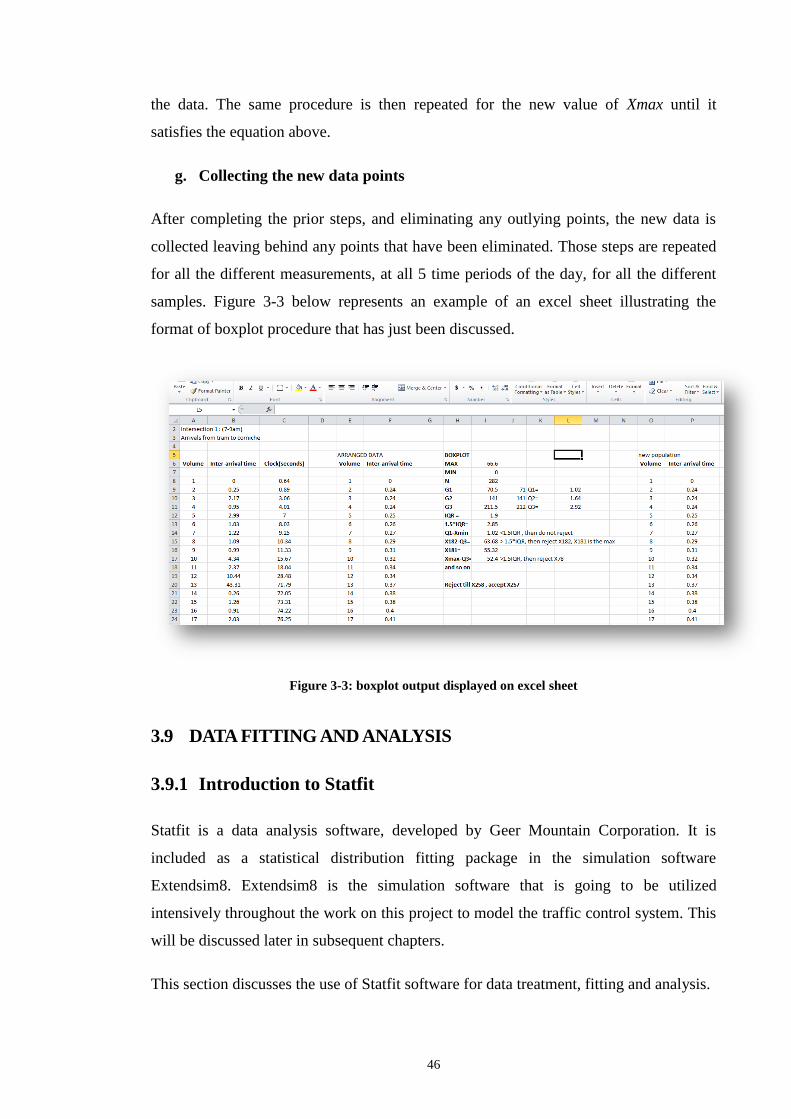
46
the data. The same procedure is then repeated for the new value of Xmax until it
satisfies the equation above.
g. Collecting the new data points
After completing the prior steps, and eliminating any outlying points, the new data is
collected leaving behind any points that have been eliminated. Those steps are repeated
for all the different measurements, at all 5 time periods of the day, for all the different
samples. Figure 3-3 below represents an example of an excel sheet illustrating the
format of boxplot procedure that has just been discussed.
Figure 3-3: boxplot output displayed on excel sheet
3.9 DATA FITTING AND ANALYSIS
3.9.1 Introduction to Statfit
Statfit is a data analysis software, developed by Geer Mountain Corporation. It is
included as a statistical distribution fitting package in the simulation software
Extendsim8. Extendsim8 is the simulation software that is going to be utilized
intensively throughout the work on this project to model the traffic control system. This
will be discussed later in subsequent chapters.
This section discusses the use of Statfit software for data treatment, fitting and analysis.

47
3.9.2 Data fitting results
Now that the box plotting procedure has been carried out on the data and the outliers
that might disturb the uniformity of the data have been removed, the population
becomes quite ready to the next step, which is the data fitting.
Each set of data, is entered to the Statfit software, which performs the statistical data
fitting and outputs a range of accepted random distributions with their correspondent
characteristic parameters (mean, St.dev, scale, shape, Etc...)
Seven intersection points are to be considered in the data pattern. Table 3-2 to Table 3-5
represent a summary of the results of statistically analysing the collected data using
Statfit.
Table 3-2: average proportions for left/right turns
Int. Type Left/Right Turn Description Proposed average proportion
1 LT PortSaid to Corniche 0.25
RT Tram to Portsaid 0.25
2 LT Aboeir to sporting tram 0.1
RT Aboeir to shatby tram 0.2
Table 3-3: road capacities for control points
Int. CP Road Capacity (vehs.)
1 1’ 80 – 100
2’ 80 – 100
2 1 (B1) 80 – 100
1 (B2) 20 – 30
1 (Com.) 20
2 60 – 80
3 90 – 120
4 20
Table 3-4: percentage time lost in signal timing
Int. CP % Time lost in signal timing
1 1’ 4 %
2’ 11.2 %
2 1 12.6 %
2 15.4 %
3 16.3%
4 N/A

48
Table 3-5: Random distributions for arrivals
Period Int A. Point Proposed distribution for
arrivals
Proposed range of average
inter-delay time (sec)
7-9am
1 1’ Weibull(1.29,3.67)
Exponential (3.33) 1
2’ Weibull(1.66,2.03)
Exponential (2) 0.5
2 1 (branch1) Weibull(1.66,2.08)
Exponential (2) 0.7
1(branch2) Weibull(1.52, 3.73)
Exponential (3.7)
2 Weibull(1.59,2.63)
Exponential (2.34) 0.5
3 Exponential (2) 1
4 N/A 0.2
9-1pm
1 1’ Weibull(1.42,4.53)
Exponential (4) 0.2
2’ Weibull(1.68,1.53)
Exponential (2.8) 0.2
2 1 (branch1) Weibull(1.66,2.05)
Exponential (3) 0.5
1(branch2) Weibull(1.37,5.25)
Exponential (4.73)
2 Weibull(1.58, 2.83)
Exponential (2.52) 0.5
3 Exponential (3) 0.7
4 N/A 0.2
1-5pm
1 1’ Weibull(1.4,2.19)
Exponential (2.5) 0.7
2’ Weibull(1.75,1.39)
Exponential (1.43) 0.5
2 1 (branch1) Weibull(1.37,1.65)
Exponential (2.5) 0.7
1(branch2) Weibull(1.41,4.07)
Exponential (3.66)
2 Weibull(1.57, 2.73)
Exponential (2.43) 0.5
3 Exponential (2) 0.7
4 0.2
5-11pm
1 1’ Weibull(1.15,7)
Exponential (5) 0.5
2’ Weibull(1.67,1.56)
Exponential (2.5) 0.2
2 1 (branch1) Weibull(1.72,2.14)
Exponential(6) 0.5
1(branch2) Weibull(1.35, 6.46)
Exponential (9) 0.5
2 Weibull (1.32, 2.8)
Exponential (2.56) 0.5
3 Exponential (2.5) 0.7
4 0.2

49
Period Int A. Point Proposed distribution for
arrivals
Proposed range of average
inter-delay time (sec)
11-7am
1 1’ Weibull(1.5,15)
Exponential (10) 0.2
2’ Exponential (7) 0.2
2 1 (branch1) Exponential (9) 0.2
1(branch2) Exponential (10) 0.2
2 Exponential (6) 0.2
3 Exponential (5) 0.2
4 0.1

50
C h a p t e r f o u r
4 ANALYTICAL MODELING AND SOLUTION
USING GENETIC ALGORITHM APPROACH
4.1 INTRODUCTION
Modelling is known as the process of developing a model of a system for the purpose of
analysis and improvement. In chapter III, Two major preliminary steps were
accomplished:
The Data collection process: A set of system parameters and variables were
measured accurately and regularly in field.
Adequate statistical analysis: Convenient treatment was carried out on the
collected data to obtain an accurate data pattern as input for the model under
construction.
This chapter devotes itself to discuss:
Analytical model formulation: The formulation of a general analytical model
that represents the traffic system in study. A general model formulation is
designed to fit for any given road network and represent any traffic control
system.
Optimization using Genetic Algorithm: This section presents “Optimization
using Genetic Algorithm approach” as the first proposed solution among a set of
other solutions discussed in this project. Based on previous work methodologies
and successful experiments adopted by researchers in the field of traffic control
analysis, Genetic Algorithm has been proven to be a very powerful and common
tool used for the optimization of traffic signal timings.

51
4.2 ANALYTICAL MODELING
“The formulation of the problem is often more essential than its solution.” This is what
the greatest scientist of the 20th
century has told us. Albert Einstein, the greatest
problem solver of all time definitely believed in the crucial importance of the model
formulation step because it gets us more acquainted with the problem, and more
qualified to find reliable solutions.
Analytical modelling, also called the process of model formulation, is the first step
towards modelling of any system. Any proposed solution throughout this project will be
based on this model formulation. The analytical modelling process encompasses several
steps that were discussed in detail in the literature review chapter. The same steps can
be summarized as follows:
- Problem Statement.
- System description and problem layout.
- Enumeration of Decision Variables: These are the control variables.
- Enumeration of system parameters: system characteristic parameters.
- Enumeration of Response Variables: The output variables which are affected by
the change in the decision variables.
- Proposed objective function(s)
- Enumeration of governing constraints
- Proposed solution approach(es).
4.2.1 Problem Statement
You simply cannot solve a problem, if you do not understand it adequately. In order to
develop a model that represents the current system under study, the engineer should
have in mind a clear understating of the existing problem. Therefore, a short and clear
problem statement should be written down as a preliminary step. The problem
statement has been discussed in detail in chapter I and can be summarized as follows:

52
Traffic congestion is a crucial problem in highly populated cities such as Alexandria,
Egypt. Due to the absence of an effective control strategy for the regulation of traffic
signal lights, a massive inflation of the vehicles’ queue lengths and the waiting times
emerges. Through field observation, the signal light timings were observed to be fixed
through all the periods of the day, which does not correspond to the randomness of the
time-fluctuating demand of vehicles.”
In addition, the main aim of the conducted study should be clarified. This should
represent the main motive behind the work. The main aim of this model is to provide a
reliable representation of the traffic control system and propose a solution approach in
order to solve the addressed problem. The solution should optimize the values of a set of
decision variables in order to minimize/maximize the specified objective function as
much as possible.
4.2.2 System Description and Problem Layout
Defining system description and problem layout is a very important step in problem
identification. This step qualifies the engineer to analyse the system surely and start the
journey of searching for feasible solutions. It is this step where the behaviour of the
system is recorded and analysed carefully.
Several system characteristics should be recorded:
A clear layout of the road network under study:
A clear layout for the road network in study should be drawn in order to visualize the
problem and understand its underlying root causes.
For example, Figure 4-1 is the layout of two consecutive intersections in Alexandria,
Egypt which we are going to study throughout this project:

53
LYCEE SCHOOL SAINT MARC
SCHOOL
TRAM
TRAM
(Underground)
PORT SAID
ELEMENTARY
SCHOOLTechnical
institute
Residential Areas
(R)
Stores
(R)
Figure 4-1: Layout of one of Alexandria’s road networks
Defining the time periods of characteristic demand patterns in the system
The day is classified into time periods/intervals having characteristic demand patterns.
This classification is left to the experience and field observation of the traffic engineer
in charge and depends basically on the location of the intersection which defines the
peak and non-peak intervals. Each period of the day has different demand patterns and
as a result, it will be assigned different signal timings in a pre-timed that are
correspondent to the demand patterns (arrival rates).
Applying this step to the two consecutive intersections studied, Field observations and
the geographic location (residential & educational facilities) necessitate that the day
should be classified into five major periods as shown in Table 4-1. All the problem
variables & system parameters that are introduced in this model are period-dependent;
however, the model will be applied in each period separately.
Table 4-1: Periods of the day
Period Time interval Peak/ non-peak
1 7-9 am PEAK
2 9-1 pm NON-PEAK
3 1-5 pm PEAK
4 5-11 pm NON-PEAK
5 11-7 am NON-PEAK

54
Phase plan defined
This step involves defining the current road network’s phase plan and
whether it needs any modification. As discussed in chapter I, A phase plan in
traffic control encompasses:
Enumeration of the control points that are (need to be) signalized. (A control
point is a point in the intersection having characteristic demand pattern and
whose flow is opposing to one of the existing streams, therefore,
signalization is needed to organize the process). Figure 4-2 shows the road
network in study after defining the control points on it.
LYCEE SCHOOL SAINT MARC
SCHOOL
TRAM
TRAM
(Underground)
PORT SAID
ELEMENTARY
SCHOOLTechnical
institute
Residential Areas
(R)
Stores
(R)(R)
1
2
3
1'
2'
4
Figure 4-2: road network with control points defined
Enumeration of the feasible states/phases. (A traffic state is a
set/combination of traffic signals rendered to a number of control points in a
specified intersection).
The phase plan process must be done considering the demand of each control point, the
geometrical design of the intersection and the accidents’ hazard.
For example, applying this step on the road network under study, we would have a
phase plan for each intersection in the road network studied:

55
SAINT MARC
SCHOOL
PORT SAID
ELEMENTARY
SCHOOL
Stores
(R)
(R)
1'
2'
Figure 4-3: layout of intersection 1
Table 4-2: Phase plan of intersection (1)
State Control Point
1’ 2’ State timing (sec)
A’ R G
B’ G R
LYCEE SCHOOL SAINT MARC
SCHOOL
TRAM
TRAM
(Underground)
PORT SAID
ELEMENTARY
SCHOOLTechnical
institute
Residential Areas
(R)
Stores
(R)
1
2
3
Figure 4-4: Layout of intersection (2)

56
Table 4-3: Actual Phase plan of intersection (2)
State Control Point
1 2 3 State timing (sec)
A R G G
B G R R
By regular field observation, it has been proved that the current phase plan of
intersection (2) is neither accurate nor reliable. Therefore, a proposed phase plan has
been proposed.
The proposed phase plan for intersection (2):
A point in the intersection which represents the left turn from control point (3) must be
identified as a control point since it satisfies the two conditions (characteristic demand
pattern, and opposing flow to one of the main streams of the intersection). This
modified phase plan will be the input for the solution scenarios proposed that will be
discussed throughout the core of this project.
Table 4-4: Proposed phase plan of intersection (2)
State Control Point
1 2 3 4 State timing
A G R R R
B R G G R
C R R G G

57
4.2.3 Enumeration of Problem Decision Variables
Decision variables, also called control variables, are the set of variables that need to be
determined in order to solve the problem. Through experimentation, the values of these
variables are changed, and the effect of this change is measured constantly. Finding the
best values for this set of variables will definitely cut off the root causes of the
addressed problem.
The general model under construction considers any road network in a single period
with (L) consecutive intersections, (N) feasible states and (M) control points, where:
Hence, the general phase plan that can be applied on any given intersection will be as
shown in Table 4-5.
Table 4-5: General phase plan of a road network
State Control Point
1 2 3 … M State timing
A {G,R} {G,R} {G,R} {G,R}
B {G,R} {G,R} {G,R} {G,R}
C {G,R} {G,R} {G,R} {G,R}
.. ..
N {G,R} {G,R} {G,R} {G,R}

58
The decision variables are then listed as follows :
( ) ( )
It is well remarkable that the cycle time of the intersection is the sum of the state
timings of the intersection. These variables are period-dependent, however we assume
the model should be applied in each period separately.
For further clarification, the road network under study will have two state timings in
intersection (1), three state timings in intersection (2) , and one cycle time for each
intersection:
( ) ( )
( ) ( )
( ) ( )
( ) ( )
( ) ( )
( )
However, an important point that must be clarified is that the state timings are not the
timings that are going to be programmed and displayed on the traffic light signals.
These are called: the traffic signal timings where:
( ) ( )
( ) ( )
The green & red timings for each control point are not decision variables. State timings
are. The green & red timings are calculated using the state timings previously
mentioned. A quick glance to the phase plan will tell the engineer how to calculate the
green & red time intervals for each control point using the state timings. For example,
using the phase plan of intersection (2) shown in Table 4-6:

59
Table 4-6: Phase plan used for signal timing calculation
State Control Point
1 2 3 4 State timing
A G R R R
B R G G R
C R R G G
Looking vertically in the column of control point (1) through the different states, it is
noticed that control point (1) exhibits green timing interval during state (A) only. Hence
Same applies for all the control point as follows:
Now, we would have another definition (equation) for the cycle time than the one
previously mentioned:
Hence, by generalizing the above equation we would have the following:
( )
Where:
( )
( ) ( )
( )
( )
( )
( )
60
4.2.4 Enumeration of system parameters
These are the characteristic parameters of the system. In a traffic control system, we
could list the arrival rates representing the demand pattern, the departure rates
representing the vehicles’ throughput (network capacity), and the geometrical capacities
of the road network.
They can be listed as follows:
Arrival rates (vehicles/sec)
( ) ( )
Departure rates (vehicles/sec)
( ) ( )
Geometrical road capacities (vehicles)
( ) ( )
4.2.5 Enumeration of the Response variables
During modelling process, it is highly recommended to differentiate between decision
variables and response variables. Response variables, also called dependant variables,
are those that change accordingly with the change of the decision variables. They are
the output values that are being affected by changing the decision variables’ values.
In the general model under construction, the response variables are listed as follows:

61
Queue lengths (vehicles)
( ) ( )
A simple equation is developed to calculate the queue length at any control point.
Assume we have a control point (1) in a given intersection, having an arrival rate of 5
vehicles/sec. The control point will certainly exhibit green & red timing intervals
consecutively ,
Then the queue length forming during (during red interval, arrivals have a value,
while departures are equal to zero) would equal to:
While the queue length forming during (both arrivals and departures have a value)
would equal to:
( )
Then, the queue length in a one cycle time ( ), would be the sum of
the two above equations:
( )
This equation can be generalized at any control point (j) in a given intersection to
represent the queue length forming during one cycle time as follows:
( )
( )
If we want to calculate the queue length forming at the end of a certain period of time
(p), then we can simply calculate the number of cycles = period interval / CT , and
multiply the number of cycles in a period (p) by the queue length forming during one
cycle.

62
Other related response variables are calculated using values of queue lengths such as
average queue length in the control point ( ) & Maximum queue length occurring in
the control point ( ).
Vehicle’s Waiting time
Average waiting time is the average time spent by the vehicle in queue until it passes
the cross line of the traffic signal departing from the intersection.
( ) ( )
4.2.6 Proposed Objective Function(s)
In the literature review phase, a large range of different proposed objective functions
has been adopted by experimenters all over the world. Some experiments tend to
minimize some crucial variables such queue lengths, waiting times, average time spent
in the system by a vehicle. Others tend to the maximization of the network’s throughput,
dissipation rates and other parameters. While some other experiments consider the
environmental approach of the problem by aiming to minimize fuel consumption and
gas emissions.
For this experiment, four objective functions are proposed. The four objective functions
are more likely to be used throughout the course of the research in different solution
approaches.
a. Minimization of Queue lengths
The first proposed objective function tends to the minimization of queue lengths. This
can be done by two methods:
Minimization of the maximum of the average queue lengths forming among
all the control points of the intersection in study. I.e. The average queue
length in each control point is computed or measured, and the aim is to
minimize the maximum of these values.

63
Minimization of the sum of the average queue lengths forming among all the
control points of the intersection in study. The average queue length in each
control point is computed or measured, and the aim is to minimize the sum
of these values.
In this equation, weights can be assigned to each control point to assign priorities for the
control points in study. For example, if there is a main stream that has a very high
demand pattern compared to other control points, larger weight is multiplied by the
value of its queue length. This leads to concentrate the minimization process on this
control point than the others. Hence, the general objective function becomes:
( )
b. Minimization of Maximum Waiting time
The second proposed objective is to minimize the maximum of the average waiting
times forming among all the control points of the intersection. The average vehicle’s
waiting time for each control point is computed or measured, and the aim is to minimize
the maximum of these values.
c. Minimization of a characteristic function
The third proposed objective is to cut off the value of a developed characteristic
function. The function is assumed to be the maximum of the products of two response
variables in each control point: Queue length & Waiting time of the control point. The
value of this function is computed in each control point, and the aim is to minimize the
maximum of these values.
)

64
The concept of this objective function will be used in the Genetic Algorithm
experiment. However, each chromosome will have this characteristic fitness function to
evaluate the goodness of the chromosome. This will be discussed in detail later on in
this chapter.
d. Minimization of the efficiency of the Average time spent in the system
The fourth proposed objective is the maximization of the efficiency of the average time
spent in system. The best average time spent in system is calculated under the best
timing conditions for each control point, and then divided by the actual average time
spent in system. This objective function will be used in the optimization using
simulation experiments and will be discussed in chapter XIII in detail.
(
)
Where:
4.2.7 Enumeration of Governing Constraints
Constraints can be simply defined as the limits of the problems’ variables. They define
the feasible range of the problem variable to ensure that the reached solution is feasible
and effective.
In the analysis of any road network, the constraints would be as follows:
Geometrical Capacity Constraint
The maximum queue length occurring in any control point in the network should not
exceed a certain characteristic limit which is the road capacity of the control point in

65
study expressed in vehicles ( ). This capacity is different from a control point to
another in a given road network.
( )
For better system performance and in order to take precautions, an estimated factor
whose value is less than one can be multiplied by the road’s capacity. This is done in
order to create a safety allowance to ensure that the maximum queue length at each
control point will never reach any close to the capacity limit.
The general equation in that case is to be:
( ) ( )
Signal timings Constraint
It is a matter of logic to notice that the signal timings should not exceed certain
specified limits. For example, it is logically unacceptable to have a very short green/red
timing interval TG of 5 or 10 seconds even if it is going to satisfy the proposed
objective function. Neither it is acceptable to have extremely long timing intervals of
more than 120 seconds for example, or cycle times that exceed a certain reasonable
limit.
These limits are estimated depending on the experience of the traffic engineer and the
careful field observation.
( ) ( ) ( )
( ) ( )
The red/green signal timings constraints can be transformed to express the limits of the
state timings (the problem decision variables) using the relationships previously
deduced from the phase plan that relate the state timings and the signal timings. For
example if , then the constraint will be:

66
( ) ( ) ( )
4.2.8 Proposed Solution Approaches
At this point, the model formulation is nearly completed. The decision and response
variables, the objective function and the governing constraints are clearly defined. The
last step of the model development is to propose a feasible solution approach and start
implementing it to solve the addressed problem. Throughout the course of this project,
three different solution approaches are adopted; Optimization using Genetic Algorithm,
Simulation, and Optimization using Simulation.
This chapter will emphasize on the first proposed solution approach which is the
“optimization of traffic signal timings using Genetic Algorithm.”
4.3 PROPOSED SOLUTION APPROACH: GENETIC
ALGORITHM
The concept of Genetic Algorithm was discussed in the literature review chapter.
However, a quick review of Genetic Algorithms and their applications should be
introduced before going through the structure of the proposed solution approach.
4.3.1 Introduction to Genetic Algorithms
Genetic Algorithms are inspired by the Darwinian process of evolution, in order to
reach the optimal or near-optimal solution for a problem. The simple concept of a G.A
experiment is the struggle between the different possible solutions called chromosomes
until the fittest and strongest solution survives at the end of the optimization process.
A simple GA experiment is an iterative process that consists of the following steps:
Selection
Cross-over/Copying
Mutation

67
First, a random population of chromosomes is produced. Each chromosome contains a
set of decision variables that represent a solution in form of genes. The fitness of each
chromosome is evaluated. The fitness is the measure of goodness of the chromosomes
of the population. The chromosomes with better fitness possess larger probability to be
selected and proceed to the next population. Selection process chooses two candidates
in order to carry out the reproduction operation.
Next, the reproduction operation is carried out either through cross over or copying
(with a considerably larger probability assigned to cross-over). Cross-over takes place
between the mating chromosomes with a specified cross-over probability to exchange
their characteristics (genes). Cross-over is used to combine two chromosomes known as
parents, to produce better children in the next population. Figure 4-5 illustrates the
cross over process.
0 1 0 1 1 0 1 0 0 1 1 1 0 1 1 1
0 1 1 1 1 0 1 00 1 0 0 1 1 1
Figure 4-5: Cross-over process
On the other hand, copying is the process of replacing the worst two chromosomes in
the population by the two selected candidates. The last step is mutation; where, random
genes of chromosomes are changed based on a pre-specified mutation probability. The
main aim behind mutation is to increase the diversity of the population and to avoid
narrowing the space of solutions. Mutation prevents the well-known local optima
problem. However, mutation probability should not be large enough to ruin the
optimization strategy and transform it into a random search. Figure 4-6 illustrates the
mutation process.
0 1 0 1 1 0 1 0
0 1 0 0 1 0 1 0
Figure 4-6: Mutation process

68
Hence, the average fitness of the population should be improved. The process is pursued
until a specified criteria is met, either a specified value for the average fitness, a
specified number of generations or there is no further improvement that can be done.
Figure 4-7 illustrates the steps of a Genetic Algorithm Experiment
Start
End
Initial Population
Evaluation
Selection
Crossover/
Copying
Mutation
Evaluation
Criteria met
?
Yes
No
Figure 4-7: G.A. steps
4.3.2 Solution approach structure: Optimization of traffic signal
timings using Genetic Algorithm
The Optimization using Genetic Algorithm is carried out using Visual Basic
Applications VBA in Excel 2010.
A. Problem layout
The solution approach will be applied separately to two consecutive intersections in
Alexandria, Egypt.

69
Intersection 1:
SAINT MARC
SCHOOL
PORT SAID
ELEMENTARY
SCHOOL
Stores
(R)
(R)
1'
2'
Figure 4.8: Layout of Intersection (1)
The control points are identified clearly on the intersection. The phase plan will be as
shown in Table 4-7: (the state timings mentioned are those currently applied in the
intersection)
Table 4-7: Phase plan of intersection (1)
State
Control Point
1 2 State timing (sec)
A R G
B G R
Number of control points = 2
Number of states = 2
Number of periods = 5
The study has been applied to different periods of the day mentioned previously.

70
Intersection 2:
LYCEE SCHOOL SAINT MARC
SCHOOL
TRAM
TRAM
(Underground)
PORT SAID
ELEMENTARY
SCHOOLTechnical
institute
Residential Areas
(R)
Stores
(R)
1
2
3
4
Figure 4-10: Layout of intersection (2)
The control points are identified on the layout. As mentioned earlier when developing
the model, control point 4 is currently not defined in the actual system. It has been
added to accurately develop a reliable phase plan. The phase plan of the intersection is
defined as shown in Table 4-8:
Table 4-8: Proposed Phase plan of intersection (2)
State Control Point
1 2 3 4 State timing
A G R R R
B R G G R
C R R G G
Number of control points = 4
Number of states = 3
Number of periods = 5

71
B. G.A Experiment parameters
Defining the Genetic Algorithm parameters accurately is a crucial factor for the success
of the experiment. It greatly boosts the possibilities of attaining an optimum/near-
optimum solution. Those parameters include the population size, required number of
generations to attain a certain level of convergence, cross-over, mutation and copying
probabilities. However, there is no general rule to define those parameters. They are
estimated based on the size of the problem, the required convergence level. They vastly
depend on experimentation, together with the experience of the experimenter in charge.
For each intersection, a G.A experiment is conducted with different parameters.
For intersection1:
Population size = 50 chromosomes
Number of generations = 3000-4000 generations
Cross over probability = 0.95
Copying probability = 0.05
Mutation probability = 0.05-0.1
For intersection2:
Population size = 50 chromosomes
Number of generations = 5000-6000 generations
Cross over probability = 0.95
Copying probability = 0.05
Mutation probability = 0.1-0.2
C. Chromosome Structure
The general model that was developed earlier is very useful in modelling the
optimization process. However, little adjustments are to be done to fit for the Genetic
Algorithm experiment.
The decision variables are the same as those listed in the developed model (state timings
and cycle time). The chromosome is composed of (N) genes carrying (N) decision
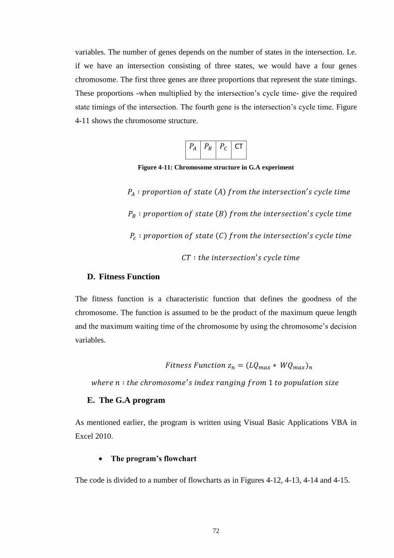
72
variables. The number of genes depends on the number of states in the intersection. I.e.
if we have an intersection consisting of three states, we would have a four genes
chromosome. The first three genes are three proportions that represent the state timings.
These proportions -when multiplied by the intersection’s cycle time- give the required
state timings of the intersection. The fourth gene is the intersection’s cycle time. Figure
4-11 shows the chromosome structure.
CT
Figure 4-11: Chromosome structure in G.A experiment
( )
( )
( )
D. Fitness Function
The fitness function is a characteristic function that defines the goodness of the
chromosome. The function is assumed to be the product of the maximum queue length
and the maximum waiting time of the chromosome by using the chromosome’s decision
variables.
( )
E. The G.A program
As mentioned earlier, the program is written using Visual Basic Applications VBA in
Excel 2010.
The program’s flowchart
The code is divided to a number of flowcharts as in Figures 4-12, 4-13, 4-14 and 4-15.

73
Start
Read
Input Data
Simulation of Car
Arrivals
Specification of
GA parameters
Chromosome
formation
Queuing
A
B
Evaluation of Fitness Function
F.F(ch) = LQmax * WQmax
Is ch ≥ pop_size
?ch = ch + 1
ch = 1
NO YES
CP = 1
(Control Point)
Sort
Generation
Selection
Reproduction
C
Is gen ≥
num_generations
?
gen = 1
gen = gen + 1
Result
End
YES
NO
Figure 4-12: Main flowchart of the GA VBA code

74
Chromosome
formation
i = 1
Sum = 0
Random Number
Generation
Store in array
num(i)
j = 1
Is i ≥ num_states
?sum = sum + num(i)
i = i + 1
Prop(j,ch) = num(j) / sum
Is j ≥ num_states
?
j = j + 1
Random Number
Generation
Y
CT(ch) =
Ctmin + (Ctmax – Ctmin)*Y
A
NO
YES
NO
YES
Figure 4-13: Chromosome formation procedure in the GA code

75
Queuing
n = 1
n: num_vehicles
Evaluation of
departure time
Tdep(CP,n)
Evaluation of Response Variables
Qlmax(CP), Qlav(CP),
Qwmax(CP), Qwav(CP)
Is n ≥
num_arrived(CP)
?
N = N + 1
Is CP ≥ num_CP ? CP = CP + 1
Evaluation of chromosome
Response Variables
LQmax(ch), WQmax(ch),
B
NO
NO
YES
YES
Figure 4-14: Queuing procedure in the GA code

76
Reproduction
Random Number
Generation
P1
CrossoverIs P1 >
Xover_p ?Copying
Random Number
Generation
P2
Is P2 > Mut_p
?
Mutation
Checking
constraints on
Decision variables
Re-evaluation of
population (FF
calculation)
C
Figure 4-15: Reproduction procedure in the G.A code
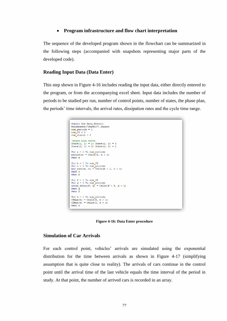
77
Program infrastructure and flow chart interpretation
The sequence of the developed program shown in the flowchart can be summarized in
the following steps (accompanied with snapshots representing major parts of the
developed code).
Reading Input Data (Data Enter)
This step shown in Figure 4-16 includes reading the input data, either directly entered to
the program, or from the accompanying excel sheet. Input data includes the number of
periods to be studied per run, number of control points, number of states, the phase plan,
the periods’ time intervals, the arrival rates, dissipation rates and the cycle time range.
Figure 4-16: Data Enter procedure
Simulation of Car Arrivals
For each control point, vehicles’ arrivals are simulated using the exponential
distribution for the time between arrivals as shown in Figure 4-17 (simplifying
assumption that is quite close to reality). The arrivals of cars continue in the control
point until the arrival time of the last vehicle equals the time interval of the period in
study. At that point, the number of arrived cars is recorded in an array.

78
Figure 4-17: Vehicles’ simulation in G.A. code
Specification of G.A parameters
In this step, the parameters of the GA are defined. These are the population size, the
desired number of generations, and the crossover and mutation probabilities.
Figure 4-18: Specification of G.A parameters in G.A code
Chromosome formation: Building population
Here, the chromosome is built up as in Figure 4-19. As mentioned earlier, the
chromosome consists of state proportions, together with the cycle time.
Figure 4-19: Chromosome formation in G.A code

79
Queuing
This step represents the queuing process that takes place throughout the system. Based
on the time of arrival of each vehicle and the phase plan sequence, the departure timings
can be calculated. Having the arrival and departure timings, the response variables can
be easily evaluated. These include the maximum and average queue lengths & waiting
times for each control point as shown in Figure 4-20.
Figure 4-20: Queuing in G.A code

80
Figure 4-21: Queuing (2) in G.A. code
Figure 4-22: Queuing (3) in G.A. code

81
Population evaluation: Fitness Function calculation
Now that we have the values of the response values for each control point in a
chromosome, the maximum queue length and waiting time among the different control
points is stored in an array. The fitness function of the chromosome is calculated as
follows:
( )
Note that the maximum queue length for a chromosome used in the FF is the maximum
of the maximum queue length among the different control points, and same applies to
the maximum waiting times.
Then, the process is repeated on all chromosomes in order to evaluate the fitness
function of each chromosome as shown in Figures 4-23, 4-24.
Figure 4-23: Fitness function calculation

82
Figure 4-24: Fitness function calculation (2)
Generation Sorting & Selection
Then, the population is sorted in an ascending order. This is because in this experiment,
the smaller the value of the fitness function, the better it is.
After that, two chromosomes are selected as in Figure 4-25 and 4-26 to pursue with the
reproduction process.
Figure 4-25: Generation sorting in G.A code

83
Figure 4-26: Selection in G.A code
Reproduction
This process is one of the crucial processes in a G.A Experiment because it ensures the
overall improvement and evolution of the population. Based on specified probabilities,
either crossover or copying takes place (with very large weight assigned to crossover
compared to copying). Crossover is the process of mating the chromosomes to produce
a better generation of children than the mating parents.
Copying is the process of replacing the selected candidates with the worst chromosomes
in the population. After that, comes the mutation process. Mutation is specified by a
relatively low percentage. It is used in order to open up new field of search and avoid
the local optima dilemma. Then, the pre-specified constraints are checked in order to
ensure that feasible solutions are attained. After creating a new population of children,
the chromosomes are re-evaluated, the generation is re-sorted and selection of new
candidates takes place. The process is repeated until meeting the specified ending
criteria as shown in Figure 4-27 and 4-28.

84
Figure 4-27: Crossover in G.A code
Figure 4-28: Copying in G.A code
Printing out the results & analysing
After meeting the specified criteria, the results are printed on an excel sheet for further
analysis as shown in Figure 4-29 and 4-30.

85
Figure 4-29: Printing results in G.A code
Figure 4-30: Printing results in G.A code (2)
F. G.A Experimentation & Results
Now that the program is running successfully, experimentation is carried out to render
the optimized decision variables. The GA optimization is applied on both intersection 1
and 2 for the pre-specified periods of the day.
Table 4-9 represents the G.A optimized state timings and cycle time during different
periods of the day in intersection 1 and 2.

86
Table 4-9: G.A results
Period
Int. State Timing 7-9am 9-1pm 1-5pm 5-11pm 11-7am
2
A 80 65 70 65 40
B 40 35 50 35 20
C 20 20 20 25 20
Cycle time 140 120 140 125 80
1
A’ 45 35 45 35
20
B’ 55 45 55 45
25
Cycle time 100 80 100 80 45
The red and green timings displayed on the light signal can be deduced from the
optimized state timings as shown in Table 4-10:
Table 4-10: red and green signals based on G.A optimized timings
Period
Int. C.Point Timing 7-9am 9-1pm 1-5pm 5-11pm 11-7am
2
1 80,60 65,55 70,70 65,60 40,40
2 40,100 35,85 50,90 35,90 20,60
3 60,80 55,65 70,70 60,65 40,40
4 20,120 20,100 20,120 25,100 20,60
Cycle time 140 120 140 125
80
1
1’ 45,55 35,45 45,55 35,45
20,25
2’ 55,45 45,35 55,45 45,35
25,20
Cycle time 100 80 100 80 45

87
4.4 EXTENDSIM8 SIMULATION OF G.A OPTIMIZED
TIMINGS
Simulation is a powerful tool to represent the system, analyse and improve its
performance. Simulation steps and procedures using Extendsim8 will be discussed in
detail in chapters V through VIII. In subsequent chapters, different simulation models
and scenarios are developed to accurately represent the system. The G.A optimized
timings are entered into the simulation model to visualize the performance of the
system, demonstrate the improvement (if any). Table 4-11 shows the simulation results.
Table 4-11: Simulation results of G.A. optimized timings
Period
7-9am 9-1pm 1-5pm 5-11pm 11-7am
Int CP.
2
1 B1 1.6 5 1.2 4 6 17 0.2 2 0.02 0.001
1 B2 1.23 4.6 1 4 3 13 1 2 0.01 0.01
1 both 10.4 17 10 17 15 22 7 19 3 10
2 20 46 15 38 15 36 10 37 2 22
3 12 24 8 19 11 20 6 18 1.13 7
4 4 24 3 20 5 25 2.5 20 0.6 11
1
1’ 5 11 5 12 7 15 3 9 1 4
2’ 7 26 3 14 5 20 3 16 0.7 7
4.5 CONCLUSIONS & RECOMMENDATIONS
The results shown above are compared to the performance of the actual performance
which is also simulated using Extendsim8 (carried out in subsequent chapters). The
simulation steps and procedures are discussed in detail in subsequent chapters.
However, it is strongly recommended to carry out a comparison between the
performance of the actual system using the currently used signal timings vs. the G.A.
optimized signal timings results obtained by G.A. experiment and visualized using
Extendsim8 simulation.

88
Charts 4-31, 4-32 and 4-33 indicate the improvement that has taken place in different
periods of the day in both intersections (1 and 2) due to the G.A optimization of traffic
signal timings.
Figure 4-31: Chart comparing the actual vs. G.A model in terms of LQav
Figure 4-32: Chart comparing the actual vs. GA model in terms of WQav
0
5
10
15
20
25
30
1 2 3 4 5
Avg
. LQ
Periods
Actual VS. GA
Actual
GA
0
5
10
15
20
25
30
35
40
1 2 3 4 5
avg.
WQ
Periods
Actual VS. GA
Actual
GA

89
Figure 4-33: Chart comparing the actual vs. GA model in terms of LQav * WQav
Hence, the overall percentage improvement can be easily evaluated for both average
queue length and average waiting time using the following equation:
Percentage reduction in Average queue length over all periods :
The average queue length in both intersections 1 and 2 has decreased by approximately
43%.
Percentage reduction in Average waiting time over all periods:
The average waiting time of intersections 1 and 2 has decreased by approximately
30.2%.
Recommendations
It will remarkable that the results are encouraging and positively reflect the success of
the G.A experiment that is conducted to optimize the traffic signal timings for the
purpose of solving the problem of traffic congestion.
0
200
400
600
800
1000
1200
1400
1600
1800
1 2 3 4 5
avg.
LQ
*WQ
Periods
Actual VS. GA
Actual
GA

90
Therefore, it is strongly recommended to:
- Implement the G.A. optimized timings in the real world system through
coordination with traffic control department in the city to ensure that the results
are reliable and effective.
- In case of the success of the implementation phase, it is strongly recommended
to apply this experiment on various critical intersections in Alexandria, Egypt in
order to generalize the success and cut off one of the main problems that
threatens the splendour of this beautiful city.

91
C h a p t e r s i x
5 MODELING AND SIMULATION OF THE ACTUAL
SYSTEM
5.1 INTRODUCTION TO COMPUTER SIMULATION
Many researchers and engineers face major problems in their systems, restricting the
opportunities to satisfy their specified objectives and goals. Those problems need to be
attended to. Sometimes they are quite simple, hence they can be solved mathematically
and analytically. However, quite frequently and in the case of real systems, those
problems offer a great degree of complexity, where the analytical solution cannot be
applicable. As a result, simulation arises.
Simulation mimics the operations of a system or process, and experiments by changing
conditions and variables within the system to understand how it behaves, and how those
alterations will impact it.
The simulation of traffic and transportation systems has started over 40 years ago, and is
an important area of discipline in Traffic engineering nowadays. During those forty
years, computer simulation has developed from a research tool of limited group experts,
to a widely used technology in the exploration, planning, designing, operating and
improvement of traffic and transportation systems. Simulation is now an everyday tool
for researchers and practitioners in all fields of the profession.
Simulation used in the fields of traffic is significant as it can study models that are too
problematic for analytical treatment, it can be used for experimental studies on a traffic
system, and to produce visual demonstrations of both present and future scenarios for
the traffic system.
Referring back to the literature review chapter, many reports, articles and conference
papers have been read and documented during the course of this project. 60% of those
references were classified according to the topic of simulation of traffic systems and
optimization using simulation. This is evidence enough that many researchers have

92
applied simulation to the problem of traffic light signal timings, in the attempt to
optimize the traffic light signal timings using specified decision criteria.
5.2 EXTENDSIM 8: SIMULATION SOFTWARE PACKAGE
Software applications that support simulation have recently grown, as the demand for
simulation is increasing, replacing all the traditional analytical solutions.
The ExtendSim8 software package has been carefully chosen to be used to perform all
the traffic system simulations, and for the optimization of the traffic light signals in this
project.
The ExtendSim package on the contrary is an easy to use, yet powerful tool when it
comes to simulation. Its environment provides the tools for all level of modelers to
efficiently create accurate, credible and usable models. The ExtendSim facilitates every
step of the simulation to be carried out in this simulation study, ranging from creation,
to validating and verifying the model, to the construction of a user interface that allows
easy analysis of the system.
ExtendSim models are built using library based iconic blocks, where each block
represents a step or calculation in the model. The software has a drag and drop interface
creation, where the blocks are placed on the model by dragging them from the library
window, and a flow is then established between the blocks. The blocks are all very
easily understood and applied, in order to model very complex systems.
In addition, the ExtendSim package provides a suite for communication tools allowing
communication with external programs such as Microsoft Excel. It also facilitates an
evolutionary optimizer which employs powerful algorithms to determine the best model
configuration, and offers options for automatic automations and debugging tools, which
all aid in validating and verifying a model, and makes it easy for the modeler to see how
the model is operating.
5.3 REVIEW ON SIMULATION STEPS
For any simulation study, there should be a set of steps and techniques to be followed
and applied as shown in Figure 5-1, to guide the analyst in creating a valid model and

93
eventually solving the desired problem. Those steps were discussed in the literature
review chapter and are listed below. They have been followed through the entire
simulation modeling of the traffic system. Their application is described later on in this
chapter.
Problem Formulation: Enumerate and define the dilemma and the required objectives
clearly.
Modelling: The construction of a model of the system by defining the decision
variables, the objective function and the feasible constraints that regulate and limit these
variables.
Data collection: The collection of the data essential to activate the model. The more the
data is accurate, the more reliable and confident the results are.
Model translation: Entering the model to the computer simulation software.
Model verification: Checking whether the input parameters and the logical structure of
the model entered in the computer replicates the real system or not. If not, the model
translation process is revised for further adjustments. Comparisons of the outputs from
the model and the actual system are carefully made, and repetition of this process is
essential for accuracy.
Simulation Experiment/ Calibration: An iterative process in which the model is run
at exactly the same actual conditions of the system, and the output results are compared
with the real system behaviour.
Validation: If the calibration results are odd, then there is something wrong with either
the modelling phase or the data collected, otherwise the sequence is continued.
Simulation runs: To run the simulation model with the alternative solutions suggested,
and analyse the results to estimate the system performance.
More runs: To check if the model needs further runs to present reliable, confident
output.
Documentation and reporting: A final report about the simulation process must be
presented to clarify the results and add credibility to the model-building process.

94
Implementation: Implementing what happened in the simulation on the real system.
Start
Problem
Formulation
Modeling Data collection
Model
translation
Simulation runs
More runs ?
Documentation
& Reporting
Implementation
NoNo
No
Run simulation
Experiment /
Calibration
Verified ?
Validated ?
Yes
No
Figure 5-1: Simulation Steps
5.3.1 Step 1: Problem formulation
The first step in the simulation study is the problem formulation. This step requires
stating and describing the problem at hand, as well as enumerating the aims and
objectives of the study. Assumptions and objectives can be made and modified
throughout the course of the traffic system study.
The problem at hand is the massive inflation of the vehicles’ queue lengths and the
waiting times throughout Alexandria, as a result of the lack of a reliable control policy
that regulates the traffic signal lights. Through field observation, the signal light timings
were found to be fixed through all the periods of the day, which does not correspond to
the randomness of the time-fluctuating demand of vehicles.
The main aim of this simulation study is to create a simulation model that accurately
represents the actual system under study, and suggest better scenarios to improve the
performance and cut off the traffic congestion problem.

95
5.3.2 Step 2: Modelling
This is the second step in the simulation study. It refers to the formulation of an
analytical model of the system by defining the decision variables, the objective function
and the feasible constraints that regulate and limit these variables.
The step of model formulation was completely accomplished in chapter V. A quick
summary of the model formulation is as follows:
A. Decision Variables
( )
B. System parameters
Arrival rates (vehicles/sec)
( ) ( )
Departure rates (vehicles/sec)
( ) ( )
Geometrical road capacities (vehicles)
( ) ( )

96
C. Response Variables
Queue lengths (vehicles)
( ) ( )
Vehicle’s Waiting time
( ) ( )
D. Proposed Objective function(s)
( )
)
(
)
Where:
E. Governing Constraints
Geometrical Capacity Constraint
( )
( ) ( )

97
Signal timings Constraint
( ) ( ) ( )
( ) ( )
( ) ( ) ( )
5.3.3 Step 3: Data collection and analysis
In chapter III, data collection and analysis process was carried out successfully. The
collected data is classified into two main categories as follows:
Numerical data
Numerical data is data that is measured or identified on a numerical scale. It is all the
quantitative input data that describes the performance of the system that can be analyzed
using statistical methods, and displayed using tables, charts, histograms, and graphs.
Numerical data patterns were presented in chapter III.
Operational and structural data
Operational and structural data describe the nature and the structure of a system. This
can be in the form of layouts and sequences to describe the operation of a system.
In this step, the system is described through both a layout of the adjacent intersections
being evaluated created on Microsoft Visio 2010, as well as a phase plan of the
intersection which describes the transition between different states in the corresponding
control points.
The layout displayed in figure 5-2 illustrates the layout of the two connected
intersections, and represents the traffic flow passing through the three control points in

98
different directions in intersection 2, and the vehicle flow in the two control points
corresponding to intersection 1.
LYCEE SCHOOL SAINT MARC
SCHOOL
TRAM
TRAM
(Underground)
PORT SAID
ELEMENTARY
SCHOOLTechnical
institute
Residential Areas
(R)
Stores
(R)(R)
1
2
3
1'
2'
Figure 5-2: Layout of the road network under study in simulation experimentation
The tables below describe the phase plans, showing the different control points in their
two states. Those phase plans have been discussed in greater detail in chapter 5.
Reference can be made to that chapter to better understand the theory behind them.
Actual phase plan for intersection 1:
Table 5-1: Actual Phase plan of intersection (1)
State Control Point
1’ 2’ State timing (sec)
A’ R G
B’ G R

99
Actual phase plan for intersection 2:
Table 5-2: Actual phase plan of intersection (2)
State Control Point
1 2 3 State timing (sec)
A R G G
B G R R
The operational sequence of traffic signalization in intersection (1) & (2) can be
demonstrated using the following state diagrams shown in Figures 5-3 and 5-4:
BA
T ≥ Ta
T ≥ Tc
T < TbT < Ta
Figure 5-3: State diagram of intersection (1)
BA C
T ≥ Ta T ≥ Tb
T ≥ Tc
T < Tb
T < Ta
T < Tc
Figure 5-4: State diagram of intersection (2)

100
5.3.4 Step 4: Model translation
Model translation is the step of entering the model into the computer. It is the process
where the model is transformed from rough ideas and formulations into computer
simulation model. This section discusses the model translation of the actual traffic
control system in study. The following snapshots will definitely be useful in clarifying
what was achieved in model translation process.
Vehicular Arrivals at Control Points
Car arrivals at control points are represented as create buttons as in Figure 5-5. The
create buttons generate items (vehicles) based on a random specified distribution. The
time between arrivals in the illustrated control point in the snapshot is exponentially
distributed. Time lookuptables are connected to the input of the create block to assign
the mean of the exponential distribution of each period.
Figure 5-5: Vehicular arrivals in simulation of actual model
Each period is defined within a specified time interval, with the correspondent mean.
The cycle ends at the end of the day, and then is repeated till the end of the simulation
runtime.

101
Queuing
A queue block follows the create block that represent the accumulation of queues. The
queue block is crucial for the simulation model as all the response variables are
withdrawn from it such as Average queue length and waiting time of the control point.
Figure 5-6: Queuing in simulation of actual model
Signalization process
Next, comes the gate block. The gate block represents the traffic light signal. When the
gate is open (having a “one” input), means green signalization, and hence vehicles are
allowed to flow. Otherwise, the gate is closed (“zero” input), signifying red
signalization and in turn restriction of vehicular flow.
All the gates of the model are connected to a general control lookuptable which defines
the sequence of operation through the phase plan. The lookuptable controls when and
how long should the gate kept open for each control point as in Figure 5-7.
Figure 5-7: Signalization in simulation of actual model

102
Inter-delay time
Right after each gate in each control point, there exist activity blocks as shown in Figure
5-8. Activity block represents the inter-delay time during vehicules’ dissipation. Each
control point has its own inter-delay time obtained through field measurement.
Figure 5-8: Inter-delay time in simulation of actual model
Exiting the intersection
Then, the vehicles exit the intersection, either directly through the exit button, or
through a select item out block where they decide to exit the intersection based on
proportions assigned in the select item out block as in Figure 5-9.
Figure 5-9: Exiting the intersection in simulation of actual model
The same procedure in buliding up the model applies on all the control points of the
intersection, only with slight differences between a control point and another.
Operational Sequence
Now, in order to demonstrate the rest of the blocks, it is recommended to quickly
review the operational logic of the model.

103
The actual model is quiet complex in operation, because as mentioned earlier, the phase
plan is inaccurate. Thus, leading to the existence of an undefined control point which
steals its state timing from the existing defined state timings.
LYCEE SCHOOL SAINT MARC
SCHOOL
TRAM
(Underground)
PORT SAID
ELEMENTARY
SCHOOLTechnical
institute
Residential Areas
(R)
Stores
(R)(R)
1
2
3
1'
2'
Figure 5-10: Layout of actual system in simulation of actual model
The actual model of intersection (2) has two states. At the beginning, state (2) takes
place, giving green signalization to CP (2) & (3) while restricting the flow of CP (1).
The vehicles taking the left turn from control point 3 are not assigned a signal timing.
Therefore, they accumulate in the middle of the intersection during the green
signalization of control point (2) & (3), and cross the road as soon as they find a chance
to stop the upcoming flow from control point (2). This means they are given a green
signal but with very low dissipation rates(because they wait until they find a chance to
cross). Then, state transition occurs In the second state, control point(1) is given a green
signal, while CP (2) & (3) are given a red signal.
However, if there is still accumulated queue in the middle of the intersection desiring to
take the left turn from the previous state, they are allowed to dissipate while holding on
the emerging flow from CP(1) till the Left turn queue dissipates. This means CP(1) is
given a red signal until the left turn queue dissipates, then they take a green signal. This
is totally an inaccurate phase plan. However, it is the actual situation and should be
modeled effectively to evaluate the current system performance. The phase plan of the
actual model would be as follows:

104
Table 5-3: Actual model phase plan in simulation of actual model
State Control Point
1 2 3 4 (does not exist) State timing
(sec)
A R G G G (with low dissipation rates)
B R(until Left turn is
empty) then G
R R G (until the flow dissipates),
then R
This logical operation is presented in the model as in figure 5-11.
Figure 5-11: Part of the simulation of actual model
The first state (read from the lookuptable) gives a “zero” to CP(1) (red signal) , and
ones to CP(2) and (3) (green signal).
An equation block shown in Figure 5-12 is added to calculate the queue length
accumulating in the left turn queues. The output of the equation block is connected to
the input of a decision (if condition) block.

105
Figure 5-12: Equation block in simulation of actual model
The decision block determines whether the queue length in the left turn is equal to zero,
or larger. If it is equal to zero, it renders a “zero”, otherwise it render a “one”. These
outputs are sent to a valuelookuptable block shown in Figure 5-13.
The valuelooktable is connected to two blocks :
Gate (A) that is in series with the gate of CP(1)
Gate (B) that is in parallel with the gate of the left turn.
If the valuelooktable has an input of “1” (means there is a queue length in the left turn),
it gives a “0” to gate (A), “1” to gate (B), and vice vers-ca.
Figure 5-13: Value lookup table in simulation of actual model
Now let us review the different states that might take place in the intersection.
If the intersection is in state (A) and there is a queue in the left turn:
State (A) means that the gate of CP(1) is closed, while those of CP(2), (3), and (4) with
low dissipation rate are open. Having a queue in the left turn, means that the decision
block will render a “one”. When sent to the value lookuptable, This would output a “0”
to Gate (A) and a “1” to gate (B).

106
Having two gates closed in series in CP(1), this means that the overall flow is given a
red signal. CP(2) & (3) are normally given a green signal. And CP(4) will select the
path of the low dissipation rate, rather than Gate(B) based on priorities set in the select
item out block.
If the intersection is in state (A) and there is no queue in the left turn.
State (A) means that the gate of CP(1) is closed, while those of CP(2), (3), and (4) with
low dissipation rate are open.
Having no queue in the left turn, means that the decision block will render a “zero”.
When sent to the value lookuptable, This would output a “1” to Gate (A) and a “0” to
gate (B).
Having one gate open and one closed in series in CP(1), this means that the overall flow
is given a red signal. CP(2) & (3) are normally given a green signal. And CP(4) will
only have the path of the low dissipation rate available.
If the intersection is in state (B), and there is a queue in the left turn
State (B) means that the gate of CP(1) is open, while those of CP(2), (3), and (4) with
low dissipation rate are closed.
Having a queue in the left turn, means that the decision block will render a “one”. When
sent to the value lookuptable, This would output a “0” to Gate (A) and a “1” to gate (B).
Having one gate open and one closed in series in CP(1), this means that the overall flow
is given a red signal. CP(2) & (3) are normally given a red signal. And CP(4) will only
have the path of gate (B) available.
If the intersection is in state (B) and there is no queue in the left turn:
Now that the queue of the left turn has totally dissipated. State (B) means that the gate
of CP(1) is open, while those of CP(2), (3), and (4) with low dissipation rate are closed.
Having no queue in the left turn, means that the decision block will render a “zero”.
When sent to the value lookuptable, This would output a “1” to Gate (A) and a “0” to
gate (B).

107
Having two gates open in series in CP(1), this means that the overall flow is given a
green signal. CP(2) & (3) are normally given a red signal. And CP(4) will have the gates
closed.
Now, intersection 2 has been modelled successfully. Intersection 1 is much more
simpler. It has its own timelookuptable block because it has its own phase plan. CP(1’)
in intersection(1) is modelled as all other control points.
Figure 5-14: Vehicular arrivals in intersection (1) in simulation of actual model
CP(2’) is also similarly modelled, however, the only difference that the input of vehicles
into CP(2’) is the sum of the exits of CP(1) and (3) of intersection (2).
Figure 5-15: vehicular arrivals to CP(2) in intersection (1) in actual model
At that point, the model translation process is now completed and the modely is ready
for experimentation runs.
5.3.5 Step 5: Verification and Validation
This model was a quite complex model, and so reaching the final state of a verified and
valid model, took a lot of effort and time. Verification and validation are the two
processes that allow simulation analysts to reach a reliable model that truly reflects the

108
reality. A lot of challenges have been faced throughout the simulation process, to reach
the desired operational, logical, and functional requirements.
There is a major different between the verification and validation processes.
Verification is concerned with making sure that the computer model is working
correctly and properly, with the right operational logic, and making comparisons with
the conceptual model. The model validation ensures that the model is a real and
accurate representation of the actual system, and comparisons must be made with the
actual system.
Verification
Throughout the modelling process, various verification steps have been carried out.
Those are as follows:
The flow of vehicles through the traffic system was monitored using the 2D
animation tool in ExtendSim8 to check that the flow is behaving is as intended.
The phase plan sequence was checked to ensure that the operational logic is
correctly being implemented.
The implementation of the” if then else” conditions in the decision blocks are
verified. These were checked to determine that the model acts correctly when it
comes to system decisions and trade-offs.
Validation
Throughout the modelling process, various validation steps have been carried out.
Those are as follows:
Using the 2D animation, detailed monitoring of every block was carried out, to
ensure the correct flow of the vehicles.
All the queue blocks were carefully tested to determine whether the model
exhibits reasonable values for queue lengths and waiting times that reflect the
situation of the actual model or not.
The select items out blocks are checked throughout the model, to determine
that the throughputs of each branch are behaving as specified in the proportion
of each branch.

109
5.3.6 Step 6: Experimentation & Results
The actual model is run under the actual circumstances and the current state timings to
evaluate the performance of the real world situation. The experimentation results are
found to be close to those captured during field observation and are presented in the
Table 5-4.
Table 5-4: Results of the simulation of the actual model
Period
7-9am 9-1pm 1-5pm 5-11pm 11-7am
Int CP.
2
1 B1 30 50 2 4 112 90 4 13 0.02 0.04
1 B2 10 20 1 3 17 55 2.2 11 0.04 0.04
1 both 19 25 12 21 18 27 13 100 4 14
2 15 30 9 25 12 31 6 25 1.4 22
3 71 84 10 22 24 30 20 30 3 22
4 11 40 4 6 7 16 4 10 0.04 0.6
1
1’ 10 15 6 14 9 17 6 15 2 12
2’ 10 24 5 20 7 23 5 20 1.6 17
5.4 CONCLUSIONS
The simulation results of the actual system in study give us a clear indication of the
weak actual performance. The actual performance exhibits massive queue lengths and
extensively high vehicular waiting times compared to normal traffic systems. Therefore,
better scenarios should be proposed in order to improve the actual performance and cut
off the traffic congestion problem from its root causes. Subsequent chapters are going to
discuss the proposed solutions to overcome this dilemma.

110
C h a p t e r s i x
6 SIMULATION SCENARIO1: PROPOSED
SOLUTION & 3D ANIMATION USING EXTENDSIM
6.1 SCENARIO1 VERSUS ACTUAL MODEL
6.1.1 The Actual model
In the actual traffic system being evaluated, the signal light timings were found to be
fixed through all the periods of the day. This does not correspond to the variability of
the vehicular demand from one period to another. As a result of the incorrect application
of the pre-timed traffic system, major problems affect the system performance. This was
obvious in the attained results of simulating the actual model at the end of chapter V. In
addition, a major error in the phase plan of the actual model was detected. The vehicular
flow turning left from control point (3) should be recognized as a separate control point.
LYCEE SCHOOL SAINT MARC
SCHOOL
TRAM
(Underground)
PORT SAID
ELEMENTARY
SCHOOLTechnical
institute
Residential Areas
(R)
Stores
(R)(R)
1
2
3
1'
2'
Figure 6-1: changes to actual system
What actually happens is that when vehicles desiring to turn left arrive at the
intersection; they start to head onto the direction of Abo-Eir, even if it is during the
green time of other control points, therefore opposing the flow of the vehicles moving
from CP (2) shatby to sporting tram and the flow of the vehicles moving from CP (1)
Abo-Eir to Corniche. This sort of free and uncontrolled flow causes blockages and
congestion in the intersection, and prevents other control points from fully utilizing their

111
green times, hence leading to great percentages of lost time. The vehicular flow of this
left turn commands their own traffic light signal, to allow their dissipation without
interrupting the flow of other vehicles during their green time. If their own traffic light
signal is installed, it will guide such vehicles waiting in queue whether they can make
the left turn yet or not, considering the entire flow and phase plan of the intersection.
6.1.2 The proposed solution '' Scenario1 ''
Due to all the problems faced and observed from the actual performance of the system
and the simulation of such a system, a solution is strived for. Since it is impossible to
change any geometric conditions of the streets or roads, a new solution is proposed that
does not require such drastic change. This is called Scenario 1. This model will still be
based on a pre-timed traffic system, where the cycle length, the phase sequence and the
signal interval timings are constant over a single period interval. The difference between
the actual model and the proposed solution is the addition of an extra control point in
intersection 2. Instead of having 3 control points in intersection 2, there are now four, as
represented in the figure below.
A traffic light signal should be installed to direct the flow of the left turn of the vehicles
from CP (4) Sporting tram to Abo Eir. This will prevent the problem of opposing any
other flows in the intersections, due to lack of control and management that has just
been described previously.
LYCEE SCHOOL SAINT MARC
SCHOOL
TRAM
(Underground)
PORT SAID
ELEMENTARY
SCHOOLTechnical
institute
Residential Areas
(R)
Stores
(R)(R)
1
2
3
1'
2'
4
Figure 6-2: CP (4) added to scenario1 in simulation experimentation

112
LYCEE SCHOOL SAINT MARC
SCHOOL
TRAM
(Underground)
PORT SAID
ELEMENTARY
SCHOOLTechnical
institute
Residential Areas
(R)
Stores
(R)(R)
1
2
3
1'
2'
4
Figure 6-3: Intersection layout in simulation of scenario 1
Table 6-1: configuration of intersection (1) in simulation of scenario1
Control
Point
Description
1' Arrivals from Saint-Marc heading to either:
Port-said street
Left turn to corniche.
2' Arrivals from Tram heading to either:
Corniche street
Right turn to port-said.
Table 6-2: configuration of intersection (2) in simulation of scenario1
Control
Point
Description
1 Arrivals from two branches of Abo-eir street to either:
Intersection 1
Right turn to sporting tram
Left turn to shatby tram.
2 Arrivals from Shatby to either:
Sporting tram street
Right turn to abo-eir.
3 Arrivals from Sporting tram to either:
Shatby tram street
Right turn to intersection 1
4 Left turn from sporting tram to abo-eir street.

113
Table 6-3: Modified phase plan of intersection (2) in simulation of scenario1
State Control Point
1 2 3 4 State timing (sec)
A G R R R
B R G G R
C R R G G
6.2 MODEL TRANSLATION OF SCENARIO1
The proposed model "Scenario1" is built on ExtendSim8. There are familiar blocks
previously identified such as the Executive, queue, activity, select item in, select item
out and exit blocks.
6.2.1 Intersection 1
SAINT
MARC
SCHOOL
PORT SAID
ELEMENTARY
SCHOOL
Stores
(R)
(R)
1'
2'
Intersection (1) is composed of two main branches (Control points):

114
Port-said branch
The cars enter the intersection from Saint Marc, and their arrivals are represented by the
create block with its lookup table. They wait in the queue block, until their traffic light
signal is green. The traffic light signal is represented by the gate block. When the
vehicles are able to flow through the gate, they have a certain dissipation rate, which is
indicated in the activity block following the gate. Finally, the vehicles have a choice of
exiting the traffic system either by going to Portsaid or turning left to Corniche. This
former flow described is represented by the select item out block, connected to exit
blocks in the figure below.
Tram to cornice branch
This branch is similar to the former branch. However, the only difference is that the
arriving vehicles reach the control points through a select item in block that sums up
different flows from intersection (1).
Figure 6-4: Portsaid branch of intersection (1) in simulation of scenario1
Figure 6-5: Tram to corniche branch in simulation of scenario 1

115
6.2.2 Intersection 2:
LYCEE SCHOOL SAINT MARC
SCHOOL
TRAM
TRAM
(Underground)
PORT SAID
ELEMENTARY
SCHOOLResidential Areas
(R)
Stores
(R)(R)
1
2
1'
2'
Figure 6-6: Intersection (2) in simulation of scenario 1
The model consists of the following branches:
1. Arrivals from shatby tram, ending by a "Select item out" divided the departures
to either sporting tram or Right turn to abo eir.
2. Arrivals from Aboeir two-branches connected by a "Select item out" composed
of three output branches :
To intersection 1 in the cornice direction.
Right turn to sporting tram
Left turn to shatby tram
3. Sporting tram branch, connected to a "Select item out" which has two outputs :
A second "Select item out" going to either straight shatby tram or right to
intersection 1.
The left turn going to abo-Eir (the new control point added in this scenario)

116
6.3 SIMULATION EXPERIMENTATION
The objective from the experimentation is to obtain a combination of signal timings of
each control point that achieves the minimum of queue lengths , waiting times and cycle
time in the intersection.
6.3.1 Runing the model
The model is run at different timings until reaching the best solution. In every period,
the timings of the proposed solution are tried at the beginning then, the results should be
observed well, the highet numbers of queue lenghts and waiting time should be adjusted
by giving the state of these numbers more timing until reaching the best solution of the
trials in almost all the control points.
Figure 6-7: Modeling of intersection (2) in simulation of scenario 1

117
6.4 RESULTS AND ANALYSIS
Table 6-4 summarizes all the state timings that results from the experimentation of
scenario1 through all the periods of the day.
Table 6-4: Results of simulation of scenario1
State/Period 7-9am 9-1pm 1-5pm 5-11pm 11-7am
A 70 60 70 60 30
B 50 40 50 60 30
C 30 20 30 30 20
A' 40 50 40 40 30
B' 40 40 40 40 20
6.4.1 Scenario1 versus the actual model
Since the actual model represents the reality, the results of each period were compared
to the actual model results in three different comparison standards.
The average queue lengths
In each period, the average queue lengths of all the control points are calculated and
compared to the averages of the actual model as shown in Table 6-5, to calculate the
percentage improvement.
Table 6-5: Comparison of scenario1 versus actual model in terms of LQav

118
The average waiting time
In each period, the averages of the averages waiting time of all the control points are
calculated and compared to the averages of the actual model as shown in Table 6-6, to
calculate the percentage improvement.
Table 6-6: Comparison of scenario1 vs. Actual model in terms of WQav
The product of average queueand waiting time
In each period, the averages of ''Averages queue*waiting time'' of all the control points
are calculated and compared to the averages of the actual model as shown in Table 6-7,
to calculate the percentage improvement.
Table 6-7: Comparison of scenario1 vs. Actual model in terms of LQav*WQav
6.4.2 Percentage improvement calculation
Percentage reduction in LQav=
Percentage reduction in WQav=

119
Percentage reduction in (LQav*WQav)=
Table 6-8: Percentage improvement values in different periods of the day for
scenario1
Periods Percentage improvement of
LQ Average
Percentage improvement of
WQ Average
Percentage improvement of
LQ*WQ Average
1 47.8% 44.5% 74%
2 -38.3% -21% -56.4%
3 52.7% 43% 79%
4 22.5% 41.5% 54.2%
5 -45% -2% -48%
The percentage improvements displayed in Table 6-8 show great decrease in, the
average queue lengths and the average waiting times and the "average queue*average
waiting time" among all the periods except the second and fifth periods of the scenario1
in compared to the actual system. The Charts 6-8, 6-9 and 6-10 represent comparisons
between the proposed solution scenario1 and the actual system.
Figure 6-8: Actual vs. Scenario 1 in terms of LQav
Figure 6-9: Actual vs. Scenario1 in terms of WQav
0
5
10
15
20
25
30
1 2 3 4 5
Avg
. LQ
Periods
Actual VS. Scenario 1
Actual
Scenario 1
0
10
20
30
40
1 2 3 4 5
Avg
. WQ
Periods
Actual VS. Scenario 1
actual
Scenario 1
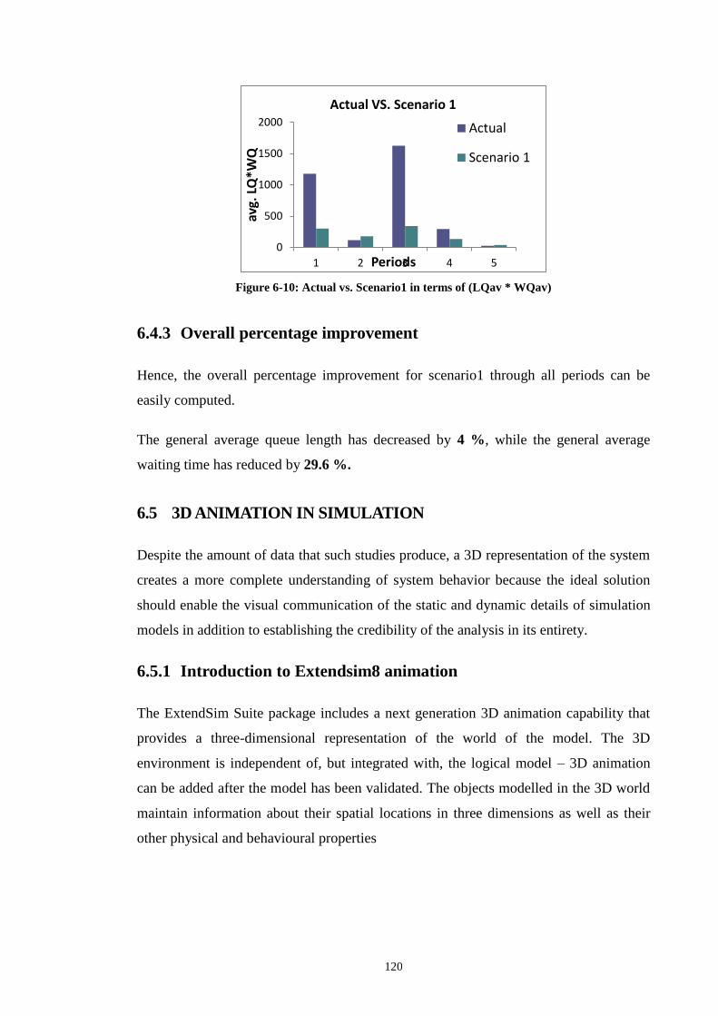
120
Figure 6-10: Actual vs. Scenario1 in terms of (LQav * WQav)
6.4.3 Overall percentage improvement
Hence, the overall percentage improvement for scenario1 through all periods can be
easily computed.
The general average queue length has decreased by 4 %, while the general average
waiting time has reduced by 29.6 %.
6.5 3D ANIMATION IN SIMULATION
Despite the amount of data that such studies produce, a 3D representation of the system
creates a more complete understanding of system behavior because the ideal solution
should enable the visual communication of the static and dynamic details of simulation
models in addition to establishing the credibility of the analysis in its entirety.
6.5.1 Introduction to Extendsim8 animation
The ExtendSim Suite package includes a next generation 3D animation capability that
provides a three-dimensional representation of the world of the model. The 3D
environment is independent of, but integrated with, the logical model – 3D animation
can be added after the model has been validated. The objects modelled in the 3D world
maintain information about their spatial locations in three dimensions as well as their
other physical and behavioural properties
0
500
1000
1500
2000
1 2 3 4 5av
g. L
Q*W
Q
Periods
Actual VS. Scenario 1
Actual
Scenario 1

121
6.5.2 3D animation of intersection (1)
It was decided to apply the 3D animation on the intersection1 of the scenario1.
SAINT
MARC
SCHOOL
PORT SAID
ELEMENTARY
SCHOOL
Stores
(R)
(R)
1'
2'
Figure 6-11 is the created 2D model in order to produce the 3D animation
Figure 6-11: 2D model used to generate 3D animation of intersection (1)
Figure 6-12 is a snapshot of the generated 3D animation:
Figure 6-12: 3D animation of intersection (1)

122
6.6 CONCLUSION AND RECOMMENDATIONS
The proposed simulation model has made improvements in the traffic system among the
day compared to the actual system,the results of the experimentations showed a
reduction in the overall queue length and vehicular waiting time.
Scenario1 which is based on dividing the day into periods each having a specific fixed
timing proved that it is more succesfull than the actual traffic systemm because the
solution has solved the variability in the demand of the cars through all the different
periods.
Concerning the intersection been studied, It is strongly recommended to use the
adjusted phase plan, previously discussed, and to apply the proposed solution for the
different periods of the day to enhance the performance of this traffic system.A reliable
control strategy is also needed to promote the awareness of the people to the new traffic
signals in alexandria.
Table 6-9 summarizes all the attained signal timings through simulation
experimentation for the road network under study.
Table 6-9: Signal timings for scenario (1)
Period
Int. C.P. Timing 7-9am 9-1pm 1-5pm 5-11pm 11-7am
2
1 70,80 60,60 70,80 60,90
30,50
2 50,100 40,80 50,100 60,90
30,50
3 80,70 60,60 80,70 90,60
50,30
4 30,120 20,100 30,120 30,120 20,60
1
1’
40,40 50,40 40,40 40,40 30,20
2’
40,40 40,50 40,40 40,40 20,30

123
C h a p t e r s e v e n
7 SIMULATION OF AN ADAPTIVE TRAFFIC
CONTROL SYSTEM
7.1 INTRODUCTION
Actuated signal control, also called adaptive or smart system, is a newly introduced
control strategy that is used nowadays in most developed countries. This strategy
greatly differs than the pre-timed control strategy in many aspects.
Pre-timed strategy: The traffic signal provides a fixed amount of green time to
each approach during a cycle. This green duration is constant over a single
period interval; however the signal timings and cycle lengths may vary from an
interval to another in order to reflect the changes in traffic volumes and patterns.
Full actuated control (adaptive): The traffic signal provides green time to each
intersection approach based on instantaneous arrivals for a cycle. Generally, as
arrivals change from cycle to cycle, the length of green time provided to each
approach also changes.
Unlike the pre-timed strategy, Adaptive traffic control systems (ATCSs) use real-time
traffic data to optimize signal timing parameters in order to minimize traffic delays and
stops. One significant difference between ATCSs and traditional pre-timed strategies is
that ATCSs can proactively respond to real-time traffic flow changes, therefore are
expected to be more efficient for signal system operations. Adaptive traffic control
systems adapt their timings based on the current demand patter. This demand patter can
be obtained through the presence of traffic sensing devices.
7.2 HISTORY OF ADAPTIVE TRAFFIC SYSTEMS
Adaptive Traffic Control System (ATCSs) is a relatively new method compared to
traditional traffic control systems. It was first introduced by Miller in 1963, when he
proposed a traffic signal control strategy that was based on an online traffic model.
However, the first real-world application did not occur until the early 1970’s when
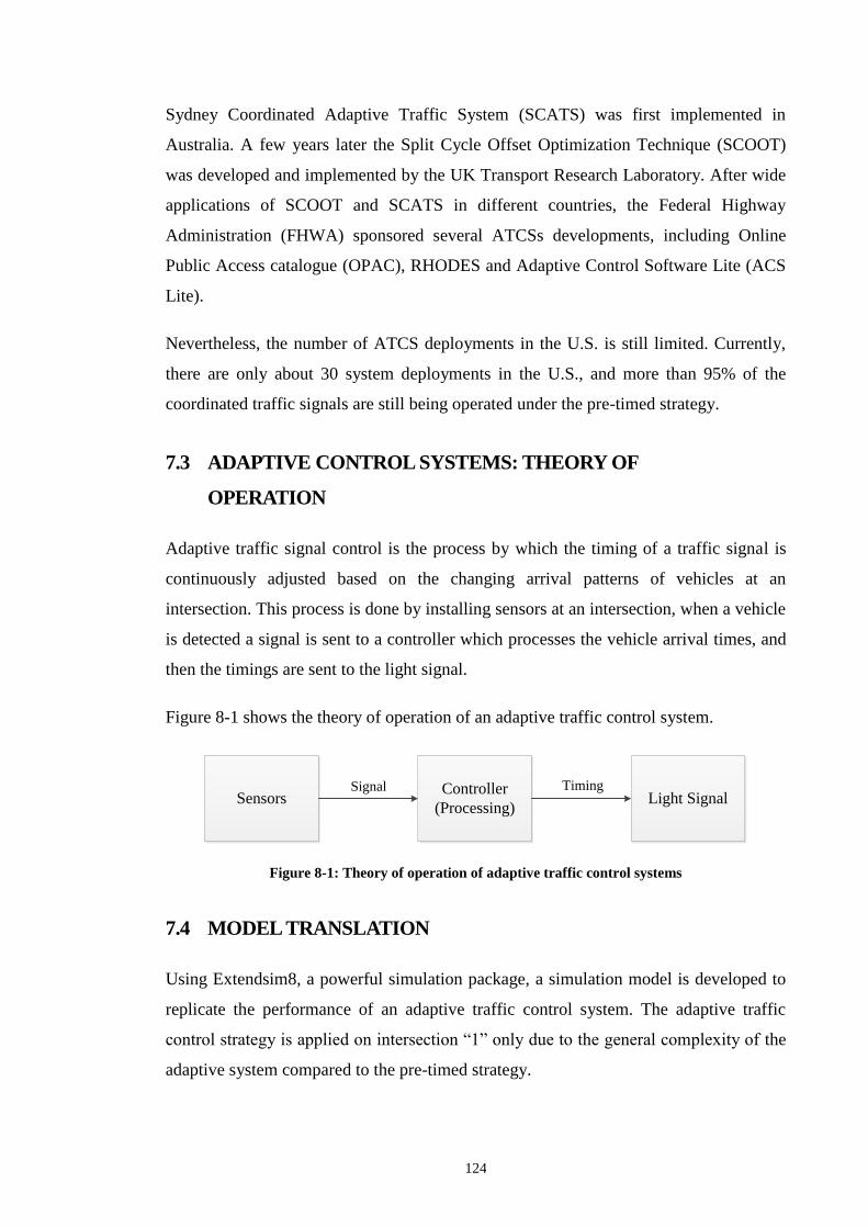
124
Sydney Coordinated Adaptive Traffic System (SCATS) was first implemented in
Australia. A few years later the Split Cycle Offset Optimization Technique (SCOOT)
was developed and implemented by the UK Transport Research Laboratory. After wide
applications of SCOOT and SCATS in different countries, the Federal Highway
Administration (FHWA) sponsored several ATCSs developments, including Online
Public Access catalogue (OPAC), RHODES and Adaptive Control Software Lite (ACS
Lite).
Nevertheless, the number of ATCS deployments in the U.S. is still limited. Currently,
there are only about 30 system deployments in the U.S., and more than 95% of the
coordinated traffic signals are still being operated under the pre-timed strategy.
7.3 ADAPTIVE CONTROL SYSTEMS: THEORY OF
OPERATION
Adaptive traffic signal control is the process by which the timing of a traffic signal is
continuously adjusted based on the changing arrival patterns of vehicles at an
intersection. This process is done by installing sensors at an intersection, when a vehicle
is detected a signal is sent to a controller which processes the vehicle arrival times, and
then the timings are sent to the light signal.
Figure 8-1 shows the theory of operation of an adaptive traffic control system.
SensorsController
(Processing)Light Signal
Signal Timing
Figure 8-1: Theory of operation of adaptive traffic control systems
7.4 MODEL TRANSLATION
Using Extendsim8, a powerful simulation package, a simulation model is developed to
replicate the performance of an adaptive traffic control system. The adaptive traffic
control strategy is applied on intersection “1” only due to the general complexity of the
adaptive system compared to the pre-timed strategy.

125
Therefore crucial changes had to be made to the existing simulation model, by adding
extra blocks. These changes are discussed below. For more information about the
original model, refer back to chapter 5.
Max & Min block
This block determines the maximum and minimum values amongst the input values.
The input connectors are connected to the queues’ blocks. The max & min block
determines the maximum or minimum value, in this case the maximum value.
Afterward the block outputs the values on output connector (1) and the respective
connector number on output connector (2).
Equation block
This block uses the set of input variables and a defined equation to update the set of
output variables. The block takes its input from the output of the max & min block, in
addition to other variables that support the equation needs. Subsequently the output
variables are connected to the lookup table block, which will be discussed later. The
equation block is demonstrated in Figure 7-2.
Figure 7-2: Equation block used to calculate the adapted signal timing in ATCs modeling
conmax
y =f (x)

126
In this case the equation block is the most important block, since it acts as the controller
that produces the signal timing. The block contains a developed equation that renders
the value of the signal timing. The equation is illustrated in Figure 7-3.
Figure 7-3: Equation used to calculate adapted signal timing in ATCs modeling
As mentioned previously, variables are added in order to maintain the equation needs,
as shown below. The third and fifth variables shown are the output values from the max
& min block. The first variable states that multiple replications will be made with a
starting condition of 20 seconds, which is constant as stated in the fourth variable. The
second variable shows the current time in seconds while the model is running, and the
last variable states the signal time.
Figure 7-4: input variables to the equation block in ATCs simulation modeling
Lookup table
Value

127
Lookup tables assign output values for correspondent input values. In this case, the table
takes the input from the equation block, looks up the correspondent value. This value is
assigned to the demand connector of one of the two gates that represent the traffic
signals, as shown in Figure 7-5.
Figure 7-5: signalization process in ATC’s simulation modeling
Figure 7-6 represents the adaptive model of intersection”1”. The two queue blocks are
connected to the max & min block to determine the maximum queue. The max & min
block is respectively connected to the equation block calculating the signal timing,
which in turn leads to the lookup table. This table determines which gate to be opened
based on the input value taken from the equation block. The process keeps repeating
itself until the run time is over.
Figure 7-6: ATC simulation modeling of intersection (1)

128
7.5 SIMULATION EXPERIMENTATION
Now that the model is developed, and all the constraints and variables are set,
calibration for each period is made in order to ensure that the model is running properly.
The model runs for a day and is distributed on five periods, each period has a model.
Calibration is achieved by running each model according to its period time, and
checking the queue block for the maximum queue length and the maximum waiting
time, as shown below. If the values are reasonable then the model is working
effectively, if not then the model needs to be modified before starting the
experimentation.
Figure 7-7: verification of system metrics in ATCs modeling
As soon as the calibration proves the effectiveness of the model, the experimentation
phase starts. Each model of the five periods is run ten times, in order to ensure the
accuracy and reliability of the results. The average queue lengths and the average
waiting times of each of the five periods, and the two control points are documented in
tables on excel sheets as in Figure 7-8.

129
Figure 7-8: Results shown on excel sheets of ATCs modeling
Table 7-9 is a summary of the averages of the total runs for each of the five different
periods, which was calculated to measure the system’s performance and to ensure that
there are no errors or exceptions among the results.
Figure 7-9: Results (2) shown on excel sheets of ATCs modeling
7.6 The Adaptive Model Versus the Actual Model
As mentioned previously, the averages of the total runs of each period are calculated for
both, the average queue lengths and the average waiting times. Afterwards, the attained
results are compared to those of the actual model. This is carried out in order to
calculate the percentage of improvement in the system performance. The calculations
are measured using the following equations:

130
-
-
- ( )
Table 7-1 shown below illustrates the improvement percentages throughout the periods
of the day:
Table 7-1: Values of percentage improvement of ATCs through all periods of the
day
periods
%
improvement
of avg. LQ
%
improvement
of avg. WQ
% improvement
of (avg. WQ *
avg. LQ)
1 70 62 88.6
2 67.3 65.3 88.4
3 42.5 55.5 74.1
4 67.3 65.7 88.2
5 61.1 64.8 86.3
As shown in the previous table, the percentages demonstrate great improvement in both,
the average queue lengths and the average waiting times among all the different periods
in the adaptive system compared to the actual system. These results prove the validity of
the model, that it runs efficiently and that the adaptive system is much more effective
than the actual model. Some graphs are illustrated for more demonstration.
All the graphs below represent comparisons between the adaptive and the actual
systems, for each of the five different periods of the day.
Chart 7-10 compares the general average queue length between the adaptive system and
the actual system.
The improvements of the adaptive system are observable in the graph below, not only in
the peak periods but in all of the periods as well.

131
0
5
10
15
20
25
1 2 3 4 5
avg.
MQ
Periods
Actual VS. Adaptive
Actual
Adaptive
Figure 7-10: Actual vs. adaptive model in terms of LQav
Chart 7-11 compares the general average waiting time between the adaptive system and
the actual system for each of the five periods of the day, and for both control points.
This graph also showed huge improvements of the adaptive system compared to the
actual system performance.
The third and final Figure 7-12 compares the adaptive system and the actual system in
terms of the general average queue length, multiplied by the general average waiting
time, at both control points for all periods of the day.
0
2
4
6
8
10
12
1 2 3 4 5
avg.
LQ
Periods
Actual VS. Adaptive
Actual
Adaptive
Figure 7-11: actual vs. adaptive model in terms of WQav

132
The improvement of this graph shows the greatest reduction in percentages among the
five periods compared to the two graphs discussed previously.
Figure 7-12: Actual vs. adaptive model in terms of (LQav * WQav)
Hence, the overall percentage improvement for the adaptive system through all periods
can be easily computed.
The general average queue length has decreased by 74 %, while the general average
waiting time has reduced by 69.2 %.
7.7 Conclusions and Recommendations
The model representing the adaptive system is developed for the purpose of improving
the traffic system’s performance. It aims to decrease the queue lengths and the waiting
times that the vehicles spend in the traffic environment. Multiple runs are performed for
five different periods over a day, and the results are quite reasonable and efficient. All
ten runs produced very similar results for each period, which proves the reliability and
accuracy of the model, as well as the effectiveness of the adaptive system.
The comparisons made between the actual system and the adaptive system, showed
huge reductions in the queue lengths and the average waiting times of the adaptive
system compared to the actual, among all the periods of the day.
0
50
100
150
200
250
1 2 3 4 5
Avg
. LQ
*MQ
Periods
Actual VS. Adaptive
Actual
Adaptive

133
The adaptive system was expected to have better performance than the actual system,
because it instantaneously adapts the timings based on the demand pattern. On the other
hand, the actual system adopts a chaotic strategy and gives fixed light signals through
all periods of the day. Therefore, the adaptive system has been proved to be better and
more efficient than the actual system.
Recommendations
Due to the experimentation and conclusions analyzed and discussed in this chapter, the
implementation adaptive traffic control system is highly recommended. However, there
are some drawbacks and requirements that should be considered in order to develop the
adaptive system in Alexandria streets. Examples of these drawbacks and requirements
are discussed briefly below.
- Awareness: there is little awareness of the high technologies involved in the
adaptive system strategy. Therefore the system should be introduced first to the
traffic department before any decisions are made.
- Feasibility: the adaptive system requires sensors as mentioned previously. Most
of these sensors require professional installation, and usually affects the
infrastructure of the roads, which is not currently possible in Egypt due to the
geometrical designs of its roads.
- Safety: some of the sensors used in the adaptive system are installed on
pavements or within easy reach to people; therefore it must be protected so it
wouldn’t be vandalized or stolen. In addition, the weather of the surrounding
environment is a critical measure since some sensing devices do not perform
effectively under bad weather conditions.
- Adequate maintenance: Sensors used in the adaptive system require
professional handling. Therefore, proper maintenance is needed regularly in
order to maintain the safety and feasibility of the sensors and the traffic system.
- Expenses: the costs of purchasing and installing the hardware devices can be
very high. Specially the controller unit which is the most important device in the
adaptive system.

134
C h a p t e r e i g h t
8 EXTENDSIM OPTIMIZATION USING
SIMULATION
8.1 INTRODUCTION
Many analysts and researchers are moving towards the path of computer simulation, as
a tool to explore the underlying system’s behaviour. However, the replication of a
system is never enough for resolving a problem. Accordingly, it is often of significant
importance to perform the optimization process on a simulation model, as a means for
determining the best set of input variable values that will improve a system’s
performance.
This is principally the aim of the following chapter, to provide the best/optimum set of
traffic signal timings for a pre-timed traffic system, in order to counteract the problem
of traffic congestion in hand.
In the previous chapters contained within the report, the actual traffic system under
study has been successfully modelled both analytically and by using computer
simulation on the ExtendSim8 software package. Furthermore, solutions have been
proposed through the optimization of the analytical model using the Genetic Algorithm
method. This chapter focuses on achieving the best solutions possible through
optimization using simulation. Both the actual model of the system and the proposed
solution presented in chapters V and VI are to be optimized.
Why use simulation optimization?
The optimization of the traffic light signals for the simulated models is performed using
a powerful tool, the ExtendSim8 optimizer. Since it would be inaccurate and very
timely to manually experiment with the model, in order to optimize the traffic light
signals to ensure the best performance, it is simpler to refer to a program that would do
so, such as the ExtendSim8 optimizer.

135
This chapter is divided up into many different sections, as enumerated briefly below:
- Introduction to optimization & Simulation optimization
This section gives a quick and brief review on the general optimization process and the
importance of optimization using simulation.
- The ExtendSim8 optimizer
The following section covers the theory of operation of the optimizer within the
ExtendSim software, as well as a brief on its benefits and limitations.
- Model formulation
This is the formulation of the general model that represents the traffic control system,
listing the objective functions, decision variables, and constraints.
- Model translation
This section describes any additional or adjusted blocks in the model.
- Optimization of the actual and proposed simulation models
This segment covers how the optimization process takes place. The actual and the
proposed model (scenario 1) are optimized using the ExtendSim8 optimizer.
- Optimizer results for actual model
- Optimizer results for scenario1
- Conclusions and Recommendations
8.2 OPTIMIZATION & SIMULATION OPTIMIZATION
Before continuing on to the solution approach using simulation Optimization on
ExtendSim8, one must refresh their memories with a general outline on optimization
and simulation optimization.

136
What is optimization?
The optimization process can simply be defined as the process by which the best or
optimum results are achieved under given circumstances. Any optimization technique
should consist of three sets of elements that are obligatory; an objective function that is
to be maximized or minimized, a collection of variables and quantities that can be
manipulated in order to achieve the specified objective function, and finally a set of
constraints that restrict the values of the decision variables. The optimization process
tries to find different solutions corresponding to the dilemma, until the best set of
variables achieved.
Various optimization techniques have been developed. The factors that determine the
optimum solution will of course vary from one situation to another. Many analysts
confer to optimization techniques to optimize costs, time required or even raw materials
used. Optimizations are also performed for obtaining both the local and global optima,
which are discussed in greater detail in the literature review chapter.
8.2.1 Simulation optimization
As specialists are increasingly using simulation as an analysis tool of performance
nowadays, a simple imitation and evaluation of the model is not enough as a proposed
solution to a given problem. Proceeding the simulation modelling, simulation
optimization should be carried out, to find the best input variable values, from amongst
all possibilities, in order to satisfy the specified objective function.
8.2.2 Simulation optimization using ExtendSim
It is always an option to optimize the model of the problematic traffic system manually,
by verifying the problem areas in the system based on outputs such as highest queue
lengths and waiting time, and allowing those control points a larger green timing.
However, this may not be the smartest of all options, because despite solving the
problem in one problematic control point in the intersection, such a solution may reflect
onto another section of the given intersection, perhaps creating complications or
bottlenecks that didn’t initially exist in the real system. In addition, such trial and error
would be cumbersome, time consuming, and maybe even impossible. Therefore is

137
necessary to search for another method to optimize the traffic light signals of the
intersection.
Simulation optimization has been used by many researchers to determine the optimum
traffic light timings. The ExtendSim8 software package is thought to be appropriate in
this case. It has previously been used to simulate both the actual and proposed traffic
system. It includes a powerful optimizer, which is utilized to optimize the model, and
find the optimum traffic light signals.
8.2.3 The ExtendSim Optimizer
ExtendSim8 software facilitates an evolutionary optimizer, which employs powerful
algorithms to determine the best model configuration. The incorporated optimizer
determines the ideal values for the parameters in a model through running the model
many times, using different values for the selected parameters, and it searches the
solution spaces until an acceptable solution is obtained. The ExtendSim tries to reach
the specified objective function, by saving the user from going through this draining
process manually.
8.2.4 Theory of the ExtendSim8 optimizer
For optimization using ExtendSim8, first the problem is stated as an objective function
or cost equation, and ExtendSim tries to minimize/maximize it. Very similar to most
optimization algorithms, where random sets of solutions are tried and evaluated, the
ExtendSim optimizer solves the models using an initial population of the possible
solutions. Each one of those solutions is then further explored, using different values for
some of decision variables. The best solution sets of those parameters are then used to
derive a new generation of slightly different but possibly better solutions. This is an on-
going process, until enough generations are reached, and the optimizer determines that
there are probably no superior solutions in sight.
However, the ExtendSim optimizer has also a few minor shortcomings. The problem of
the local optima that has been covered in the literature review may occur. The
optimization algorithms are unable to specify exactly when the best solution has been
found. As long as the objective function is showing a decrease/increase in its value, the
optimization process continues, but when the process terminates, there is no assurance

138
that the minimum/maximum value returned is in fact the optimum. No optimization
algorithm is guaranteed to produce the best answer in a limited time and that is why
running the optimization procedure several times is of great importance.
Furthermore, the optimization model needs to run continually, and this may take
extremely long times particularly with larger models, such as the traffic model under
study.
8.3 MODEL FORMULATION
Before starting with the steps of optimization, the problem in hand must be clarified,
and all the decision variables, objective functions and constraints must be stated in order
to fully understand the specified traffic system.
The entire model formulation concerning the whole traffic study is described in great
detail in chapter IV for both the actual and proposed solution. This chapter only focuses
on the decision variables, the objective functions and system parameters regarded by the
optimization process for two simulation models, the actual and proposed solution. For
further reading on the proposed model and phase plan refer to chapter VI.
8.3.1 Problem Decision Variables
The decision variables are vital as they are a set of independent variables that need to be
experimented with to solve the problem. Changing the values of a system’s decision
variables will affect the behaviour of the system, and the effects of those changes are
evaluated. The best value for the set of those decision variables can be found through
optimization, in order to try to overcome the causes of the traffic system problem.
The general model under construction considers any road network with (L) consecutive
intersections, (N) feasible states and (M) control points, where:
The

139
The general phase plan that can be applied on any given intersection is described in
detail in chapter IV, and reference can be made to it.
The decision variables for the general case are stated as follows :
( )
The cycle time of the intersection is the sum of the state timings of the intersection:
For the more specific problem of the two intersections under study for the proposed
phase plan as an example, there will be two state timings in intersection (1), three state
timings in intersection (2) and one cycle time for each intersection:
( ) ( )
( ) ( )
( ) ( )
( ) ( )
( ) ( )
( )
( )
An important fact must be pointed out regarding the state timings. The state timings just
described are not the respective green and red timings that are to be displayed on the
traffic light signals. Those are called the traffic signal timings where:
( ) ( )
( ) ( )
The green and red timings for each control point are not decision variables for the
optimization process. Instead, they are can be related to the state timings through a
series of calculations. The exact derivations of those calculations are covered in chapter

140
IV. The equations below provide an example of the equations that tie together the state
timings and the traffic signal timings for intersection two in the proposed solution.
Another formulation for the cycle time can be now derived.
Hence, by generalizing the above equations we would have the following:
( )
For both intersection 1 and 2 in the actual model, and intersection 1 of the proposed
solution, only two states exist. As a result the separate state timings will be equal to the
green and red timing interval respectively.
8.3.2 System parameters
The system parameters are the characteristic parameters of the system. In a traffic
control system, the parameters specific to it include the arrival rates of the cares, the
departure rates, as well as the geometric capacities.
However, in the corresponding optimization study, both the vehicle arrival and
departure rates do not play a large role when preparing the formulation for the
optimizer. Only the maximum capacities of the roads at each control point are
considered. The road capacity can be listed as shown below.
( ) ( )

141
8.3.3 System Response variables
For the given model the response variables are as recorded:
- Queue lengths (average and maximum)
( ) ( )
- Vehicle’s Waiting time
The Average waiting time is the average time spent by the vehicle in queue until it
passes the cross line of the traffic signal departing from the intersection.
( ) ( )
8.3.4 Objective Function
Maximization of the average vehicles’ time in system efficiency:
This proposed objective function tends to maximize the average efficiency of the time a
vehicle spends in the system. The time in system is the difference between the times that
a vehicle enters the system in any given control point, and the time that it exits it. Based
on this definition, the vehicle’s time in system is to be measured at each control point
for both intersections. The time in system will encompass all details about the vehicles
waiting time, the average queue length, maximum queue lengths and so on.
(
)

142
In this equation, certain constants are calculated for at each control point of both
the actual and proposed solution, through a certain experimentation approach, which is
described further on in this chapter.
8.3.5 The system’s Constraints
In the analysis of any road network, the constraints would be as follows:
- Capacity Constraint
The maximum queue length occurring in any control point in the network should not
exceed a certain characteristic limit which is the road capacity of the control point under
study expressed in vehicles ( ). This capacity differs between every other control
point in the two adjacent intersections evaluated.
( )
- Signal timings Constraint
There are certain logical considerations that need to be taken into account. The signal
timings to be optimized should be within certain ranges. The state timings and cycle
times should all have upper and lower limits that they cannot exceed. These limits are
estimated basted on careful field observation.
( ) ( ) ( )
( ) ( )
The red/green signal timings constraints can be transformed to express the limits of the
state timings (the problem decision variables) using the relationships previously
deduced from the phase plan that relate the state timings and the signal timings. For
example if , then the constraint will be:
( ) ( )

143
8.4 MODEL TRANSLATION
The optimization experiments in this chapter are based on maximizing the efficiency of
the vehicle’s average time in system. In order to compute the average time spent in the
system by a vehicle in each control point, some minor modifications need to be made in
the model.
A few new library blocks are added, in addition to the original model built, whether it is
the actual or proposed model. For further information about the blocks used to build the
traffic system model, and the model translation, refer to chapter V.
The table below represents each additional block placed in the model, or modifications
made to existing blocks, to carry out the optimization process. Their purpose and
function specific to the traffic system model are described. All those blocks have
multiple functions and theory of operations, which can be read about in the appendix of
blocks, however here they are discussed in the context of the proposed problem.
Block Function
Optimizer
Using evolutionary strategies, the optimizer searches for the best set of
decision variables (state timings in this case), to maximize the time in
system efficiency, considering the specified constraints
Create
The create block has been described before in the model translation
section. However, in this chapter, an important property of the create
block is changed, in order to measure the time the vehicle spends in the
system.
From the create block’s options tab, a new timing attribute known as
‘Time IN’ is assigned to the vehicles as they enter a control point. This
timing attribute will also be assigned to the respective information block,
described next.
Information
block
This block is used to calculate the time that a vehicle spends in the
system. It is placed in six different sections of the traffic system model,
before the vehicle exits the system.
The timing attribute established in the create block, that measures the
time a vehicle enters a certain control point, must be selected in the
information block’s dialog.
This means the attribute will be set to the time that the Create block
generated the item, Time In. When the item arrives to the Information
block, the value of that attribute will be subtracted from the current time.
The difference is the vehicle cycle time.

144
Mean&
Variance
It is used to calculate the mean of the time spent in the system reported
in information block. It is connected to the cycle time output of every
information block.
Equation
This equation block is only placed at one point in the model. The traffic
model consists of two intersections linked to each other. There is a point
in the second intersection where the arrivals of the cars, depends on the
departures of the cars in the intersection before it. Hence, an items
equation block is used, to assign a new attribute Time In2, to measure
the time the vehicle spends in the second intersection only.
The figure below represents all the additional blocks added to the model whether it
being the actual or proposed model. There are six different points in the model where
the average time spent in the system by a vehicle is measured. The red squares in the
figure below represent the different information blocks used to measure the vehicle’s
time in system at 6 different points, and each information block has a mean and variance
block connected to it. Notice also the position of the equation and optimizer blocks.
The following figure represents intersection 1 of the traffic system. It describes how the
certain parameters in the equation block, as well as the create blocks are set and
recognized with the information blocks.
Information Block Equation block
Optimizer block

145
8.5 OPTIMIZATION OF THE ACTUAL AND PROPOSED
MODEL
Optimization is carried out on both the actual and proposed models. Optimization runs
have been performed for an entire complete day, as well as for every period of the day
separately.
8.5.1 The steps for optimizing the traffic light signals
There are certain steps and procedures that need to be followed when performing
optimization on a simulation model. The following steps described below are followed,
Optimizer block

146
in order to optimize the model representing the traffic system of the two adjacent
intersections.
The first optimization experiment was performed on the actual model, followed by
experiments on the proposed solution scenario1. Nevertheless, the same general steps
are applied to all optimization runs, whether it being the actual model, proposed model,
or different periods of the day. The steps described are a general case applied to any
optimization experiments conducted, with a few examples demonstrated to clarify the
process.
1. Add the optimizer block to the model.
After making all the necessary modifications to the models in order to correspond to the
objective function, the optimizer block is placed from the value library and onto the
model. Inside the optimizer block’s objectives tab, is a variables table, for entering the
all the decision and response variables. There is also an equation pane under the
variables table for entering the objective function.
2. Determining the form of the objective function
Before all the variables can be added to the optimizer block, the variables that are
significantly important need be clarified. These variables depend on the objective
function. The optimizer will try to reach a goal by changing the values of decision
variables, and evaluating certain response outputs. By deciding on the basis of the
objective function, the factors and variables that are to be optimized or affected by the
optimization process are clarified, and therefore added to the optimizer block.
As discussed in the model formulation, the optimization experiment aims to maximize
the efficiency of the average vehicle’s time in system. This is achieved through a simple
ratio. It is the average of the sum of the best average time in system possible for each
control point divided by their respective actual time in system. This objective function is
also based on a certain maximum queue length respective to the road capacity that
cannot be exceeded for each control point.
(
)

147
The best times in the system need to be measured, and are used as constants in the
objective function equation. This is done through a trial and error process, where for
each control point, the best conditions are set. In order to achieve the shortest time that
vehicle can spend in the system, the time that traffic light is green is increased, and the
time that it is red is decreased. In addition, for the actual model the exception gate in
intersection 2 is removed to prevent any vehicles turning left during Abo Eir’s green
time. Chapter V can be referred where the model is translated and described, and the
concept can be better clarified.
The procedure is repeated for all control points in all the models one at a time, with
identical conditions each time, assigning 100 seconds for green light, and 20 for red
light. The average time the vehicle spends in the system is observed for each section and
noted down. Those constants differ from each model, depending on the period of the
day that the model represents. Figure 8-1 is an example of the numbers recorded in an
excel sheet, for the proposed scenario in the first period.
Figure 8-1: Calculation of CTbest in
optimization using simulation

148
3. Determine all the variables the objective function needs, and add them to
the optimizer block
Any variables and parameters are placed into the optimizer block by a process known as
clone dropping. It simply uses a clone button, to drag clones of the desired variables,
into the optimization block. This allows the optimizer block to read and change values
of that variable in the model, allowing it to explore different feasible solutions during
the run.
As discussed in greater detail before, the decision variables in this case are both the state
timings and cycle times for the two intersections, differing and depending on the phase
plan of either the actual or scenario 1 models. The response variables are the average
time in system for each segment of the system, as well as the maximum queue lengths
forming at each control point. The maximum capacities of each control point need to be
considered.
The list below represents all the different variables that are placed into the optimizer
block, and how they are named, for the actual model, as an example. For the proposed
model, there will be one additional decision variable, in intersection 2. Refer back
to the model formulation section of this chapter to better remember what each variable
stands for.
- For intersection 1 there are the two decision variables,
- For intersection 2 there are also two decision variables,
- There are nine different response variables throughout the entire system,
indicating the maximum queue length at each control point represented as:

149
- There are six other different response variables indicating the average vehicle
time spent by the vehicle at each segment of the traffic system, and they are
represented in the optimizer block as follows:
Figure 8-2 represents the position of the different control points for the proposed phase
plan. This clarifies which segments in the intersections the response variables are
obtained from. The numbers on the layout, correspond to the numbers found in the
response variables names. 2’ and 1’ represent the numbers 5 and 6 respectively.
LYCEE SCHOOL SAINT MARC
SCHOOL
TRAM
TRAM
(Underground)
PORT SAID
ELEMENTARY
SCHOOLTechnical
institute
Residential Areas
(R)
Stores
(R)(R)
1
2
3
1'
2'
Figure 8-2: Layout of the intersection under study in optimization using simulation
Using the clone layer tool, all the variables are dragged onto the optimizer block. Once
the optimizer block’s icon is highlighted, the mouse can be released, and this ensures
that the variables have been successfully placed. The name of the variable is also
changed as required.
For the case of cloning a variable contained in a table, the entire table must be cloned
and dropped into the optimizer and the row and column indexes need to be entered and
separated by a comma. Take for instance the cumulative state timings, they are found in
a lookup table. This block is opened, and using the clone layer, the data table in the
dialog box containing all the state timings is dragged onto the closed optimizer block.
The row and column within the optimizer block must be determined for this table, to
indicate the cell to use. In the case of intersection 2, there are two state timings, of both

150
A and B to be cloned, with coordinates of (1, 0) and (2, 0) respectively. This process is
repeated for ALL decision variables found in look up tables.
As for single parameters, such as the maximum queue lengths at each control point, and
the average cycle times, the dialogue box for each queue or information block is
opened, and the single value representing the variable is directly cloned onto the closed
optimizer block, without having to determine the row or column.
The figure below describes the process of cloning the maximum queue length from a
queue block and into the optimizer. The same is done for all the maximum queue
lengths and average time in the system. The average time in system are collected from
the mean and variance block.

151
The clone dropping process is continued, until all the variables are placed into the
optimizer block.
4. Setting the limits for the variables
This step is a vital step in order to allow the optimizer to differentiate between both the
decision variables, and the system parameters or response variables.
The variables that the optimizer will try to change are those that have specified limits
set for them. As for the variables without limits, they are considered to be outputs from
the simulation, and the optimizer will not try to change them. Therefore, it is necessary
that after all the decision variables are cloned, their maximum and minimum limits are
set.
Logically, the traffic signal lighting time should not be smaller than 20 seconds, neither
larger than 90 seconds, as usually the time set on the digital screen is a 2 digit number.
Below is an example on the limits set for the decision variables for the actual model:
- 20
- 40
- 20
- 60

152
The figure below represents how those limits should be entered in the optimizer
objectives tab.
5. Entering the objective function
At this stage, all the variables are clarified, and all the limits are entered. The objective
function can now be entered in the standard form in the equation pane. The objective
functions can minimize cost or maximize profit such as in the case of this experiment.
The profit is maximized, because as the shortest average time in system is divided by a
smaller actual average time in system, than the profit increases and vice versa.
In this optimization experiment, the objective function is written in the form of an IF
ELSE equation. As mentioned before, the vehicle’s time in system in general depend on
the maximum queue length or capacity allowed for each control point, therefore soft
constraints specifying maximum number of vehicles in queue must be placed.
The objection function states that if any of the maximum queue lengths set are
exceeded, than the maximum profit will equal the average of the sum of the best
average times in system divided by their respective actual average time in system, for
every given control point. Otherwise, if the soft constraints are satisfied, then the
maximum profit is equal to the former, but multiplied by 100. The maximum queue
lengths for each queue in the system are represented in Figure 8-3.
Figure 8-3: The objective function of the optimization using simulation model
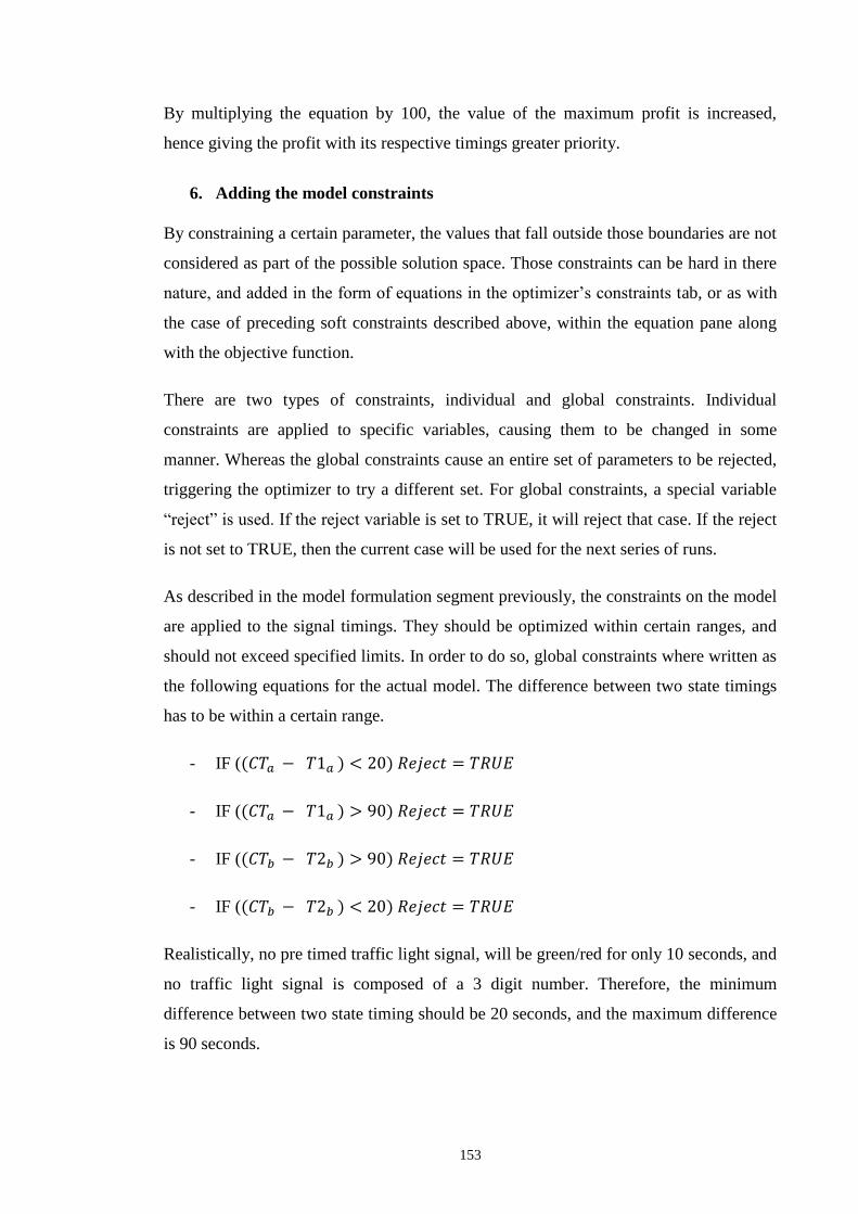
153
By multiplying the equation by 100, the value of the maximum profit is increased,
hence giving the profit with its respective timings greater priority.
6. Adding the model constraints
By constraining a certain parameter, the values that fall outside those boundaries are not
considered as part of the possible solution space. Those constraints can be hard in there
nature, and added in the form of equations in the optimizer’s constraints tab, or as with
the case of preceding soft constraints described above, within the equation pane along
with the objective function.
There are two types of constraints, individual and global constraints. Individual
constraints are applied to specific variables, causing them to be changed in some
manner. Whereas the global constraints cause an entire set of parameters to be rejected,
triggering the optimizer to try a different set. For global constraints, a special variable
“reject” is used. If the reject variable is set to TRUE, it will reject that case. If the reject
is not set to TRUE, then the current case will be used for the next series of runs.
As described in the model formulation segment previously, the constraints on the model
are applied to the signal timings. They should be optimized within certain ranges, and
should not exceed specified limits. In order to do so, global constraints where written as
the following equations for the actual model. The difference between two state timings
has to be within a certain range.
- IF (( ) )
- IF (( ) )
- IF (( ) )
- IF (( ) )
Realistically, no pre timed traffic light signal, will be green/red for only 10 seconds, and
no traffic light signal is composed of a 3 digit number. Therefore, the minimum
difference between two state timing should be 20 seconds, and the maximum difference
is 90 seconds.
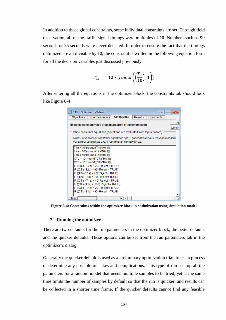
154
In addition to those global constraints, some individual constraints are set. Through field
observation, all of the traffic signal timings were multiples of 10. Numbers such as 99
seconds or 25 seconds were never detected. In order to ensure the fact that the timings
optimized are all divisible by 10, the constraint is written in the following equation form
for all the decision variables just discussed previously:
((
) )
After entering all the equations in the optimizer block, the constraints tab should look
like Figure 8-4
Figure 8-4: Constraints within the optimizer block in optimization using simulation model
7. Running the optimizer
There are two defaults for the run parameters in the optimizer block, the better defaults
and the quicker defaults. These options can be set from the run parameters tab in the
optimizer’s dialog.
Generally the quicker default is used as a preliminary optimization trial, to test a process
or determine any possible mistakes and complications. This type of run sets up all the
parameters for a random model that needs multiple samples to be tried, yet at the same
time limits the number of samples by default so that the run is quicker, and results can
be collected in a shorter time frame. If the quicker defaults cannot find any feasible

155
solutions, then better defaults are tried. The better results they increase the number of
samples, as a result increasing the time of run.
There are two other parameters that are especially important to the convergence of the
optimization, the maximum samples per case, and when to terminate the run.
- The maximum samples per case are simply the maximum number of runs
averaged to get a result. For random models such as the one under study, this
number needs to be high enough to get a useful value. In the quicker defaults, a
maximum of 5 samples is run, whereas for the better defaults it is 100.
- Terminate if the best and worst within (%): this value is used to examine the
current population of the results, to see if they are within a specified percentage
of each other. This percentage causes the optimization process to continue until
the population converges closely to that value, increasing the chances of a more
optimum answer. For quicker defaults, the optimization terminates when the best
and worst results are within 0.9, and for the better results it is at 0.995.
The optimizer also checks the convergence after a certain number of specified cases.
Figure 8-5 displayed below represents the run parameters, for the quicker default of a
random model.
Figure 8-5: run parameters in the optimization using simulation model

156
The optimization is run by clicking new run in the optimizer’s dialog. As the
optimization process takes place, the optimizer sorts the results based on the objective
function, which is to maximize the profit, and better solutions replace inferior solutions
in the population table. Therefore the results are always arranged in descending order.
After the run is terminated at a certain convergence, the results appear in the same way
represented in the figure 8-6.
Figure 8-6: results found in the optimizer block in optimization using simulation model
8. Interpreting the results
The results tab will show the entire population of solutions resulting from the
optimization run, sorted with the best solution in the first row.
The only values shown are for the decision variables results, as the optimizer tries
different values for the state timings and cycle times. Results are also displayed for the
maximum profit resulting from the optimization run. All the other variables are blank as
they are outputs from the run.
The best solution set for the selected parameters or decision variables are automatically
placed into the model, so that a simulation run can be performed, to evaluate the
performance of the optimized traffic system.

157
8.6 EXPERIMENTATION AND RESULTS
8.6.1 Optimization of the traffic light signals for the actual
model
Optimization of the entire day
The first optimization run was performed on the actual model, using both quicker and
better defaults. It was run for the entire day with the differing arrival rates for all
periods. Since the pre-timed system in Alexandria in reality is incorrectly applied and
the timings are set randomly, trying to find one set of optimum signal timings to be
fixed throughout the entire day is thought to be appropriate for the current real case.
However, whilst interpreting the results, it was discovered that no feasible solutions
have been found. The maximum profit is a small number as shown in the figure below,
indicating that the soft capacity constraints entered in the objective function have been
violated, and the optimizer was unable to find a solution to satisfy the entered
capacities.
This is a logical result, and it indicates that in fact the real system and management of
the intersection under study is operating incorrectly, as a result creating extreme traffic
congestion.
Optimization of the individual periods
As a solution to this problem, different models where replicated. Each one represents a
different period of the day. As covered before in the report, each period of the day has

158
different vehicle demand and arrival rates, therefore each one of the models has
different arrival rates, ones that correspond to the period of the day it represents.
Since there are no feasible solutions to fixed signal timings throughout the day as a
whole, this experiment aims to apply a correct pre-timed system. In this case the traffic
signal timings are fixed and pre-determined. However, every period of the day has its
own set of fixed timings, corresponding to the vehicle demand during that period. As
the day has previously been classified into 5 different periods in the report, 5 different
models were run.
Table 8-1 represents the results obtained for periods 1,2,3,4, and 5, of the actual model.
They are all summarized indicating the different values obtained for the decision
variables and the maximum profit corresponding to those timings.
Note that for period 1 and 3, the maximum profit is a small number. This is because the
optimizer has been unable to reach a feasible set of solutions for the signal timings, that
satisfy all the constraints entered. Again, those results make logical sense since period 1
and 3 are the two peak periods with the highest arrival throughout the day, probably
representing long queue lengths.
Table 8-1: State timings obtained in optimization of actual model
PERIOD 1 2 3 4 5
Int. 2 80 50 80 80 80
100 70 100 100 100
Int. 1 80 20 80 70 20
100 100 100 90 100
Max. profit 0.638 79.5 0.62 87.5 78.5
Table 8-2 represents the conversion of those values into the actual state timings using
the equations and relationships stated and explained earlier on in this chapter, in the step
of entering the decision variables into the optimizer block.

159
Table 8-2: State timings obtained in optimization of actual model
Period
Int. State Timing 1 2 3 4 5
2
A 80 50 80 80 80
B 20 20 20 20 20
Cycle time 100 70 100 100 100
1
A’ 80 20 80 70 20
B’ 20 80 20 20 20
Cycle time 100 100 100 90 40
Using the equations and relationships that link the state timings with signal timings, the
actual red and green timings that are to be displayed on the traffic light signals are
calculated. Such a conversion is briefly described in this chapter in the model
formulation section. For greater knowledge about the derivation of such equations, refer
to chapter IV. Table 8-3 summarizes the red and green timings.
Table 8-3: red and green timings obtained through optimization of actual model
Period
Int. C.P. Timing 7-9am 9-1pm 1-5pm 5-11pm 11-7am
2
1 20, 80 20, 50 20, 80 20, 80 20, 80
2 80, 20 50, 20 80, 20 80, 20 80, 20
3 80, 20 50, 20 20, 80 80, 20 80, 20
Cycle time 100 70 100 100 100
1
1’ 20, 80 20, 80 70, 20 20, 20
2’ 80, 20 80, 20 20, 70 20, 20
Cycle time 100 100 90 40
The results obtained from evaluating and measuring the systems performance for each
optimized model and time period were noted on an excel sheet, and summarized in
tables 8-4 and 8-5. The average queue lengths and average waiting times for each
control point and period are represented in the first table and average vehicle time in
system in the second. For the layout of the intersections and the position of the control
points, chapter VI or VII can be referenced.

160
Table 8-4: performance metrics from the optimization using simulation of actual
model
Period
7-9am 9-1pm 1-5pm 5-11pm 11-7am
Int. CP.
2
1 B1 4.5 13.6 1 2.6 6821 20457 0.02 0.13 0.007 0.07
1 B2 3.6 13.6 0.5 2.6 4192 15440 0.02 0.15 0.006 0.07
1 both 13 21.8 9.4 15.4 20 56 6.5 27 5.9 31.9
2 1.1 2.6 1.4 3.6 1.04 2.6 1.1 2.8 0.4 2.2
3 2.2 2.2 2 3 2.2 2.2 1.2 2.3 0.5 2.1
4 2.8 5.6 0.7 2.2 2.8 5.6 0.2 0.8 0.01 0.1
1 1’ 14.2 25.9 1.7 3.6 13.3 30.9 8.8 35.7 25.6 37
2’ 2.1 2.4 29 37.8 1.9 2.4 2.3 2.4 0.42 2.7
Table 8-5: performance metrics (2) from optimization using simulation of actual
model
Period
7-9am 9-1pm 1-5pm 5-11pm 11-7am
Int. CP.
2
1 35.4 18 17994 27.1 31.96
2 3.1 4.1 3.1 3.3 2.7
3 2.4 3.3 2.5 3.3 2.2
4 14.8 14 14.9 12.8 13.2
1
1’ 26 3.8 31 36 37.2
2’ 2.6 40 2.6 2.6 2.9
The optimized actual model versus the actual model
By finding the average of the average Queue lengths, waiting times, and vehicle cycle
times for the entire traffic system, at each period of the day and combining this data, the
percentage improvement of the certain parameters is calculated. Comparisons are made
between the performance of the actual system using the current traffic signals, and the
optimized actual model.

161
The equations used to measure the percentage are as listed.
-
-
-
Table 8-6 represents the improvement percentages.
Table 8-6: Improvement percentages obtained
Periods % improvement
of avg. TS
% improvement
of avg. LQ
% improvement
of avg. WQ
1 35 75 69.6
2 42.5 6.7 38.4
3 -13.9 -3722 -12355
4 61.7 66.5 68.1
5 26.8 -173 13.2
Note that there are large negative percentages. This means that no improvements have
been made in the overall system, but rather an increase in the queue lengths, waiting
times and times in system. This is due to the fact that the optimizer was unable to reach
a feasible solution for period 3. However, despite the fact that the optimizer was also
unable to reach the best or optimum solution for period 1, there has been an
improvement in the systems performance in all parameters, when compared with the
real performance of the adjacent intersections.
Since a couple of the periods produced infeasible solutions, comparing those results
with the actual performance obviously shows slight improvement at certain control
points, and major problems in others. Such comparison is not really practical or
accurate. There is no basis or criteria for comparisons. This is why the results of the
optimization of the proposed scenario offer greater importance.

162
8.6.2 Optimization of the traffic light signal’s results for the
proposed solution (scenario 1)
The second optimization experiment aims counteract the problems faced when
optimizing the actual model. Therefore it was thought appropriate to try and optimize
the modified traffic model, which is scenario 1. In order to understand the difference
between both the proposed and actual models, both specific to the theory of operation
and model translation, refer to chapters V and VI.
Briefly, this difference between them is basically the phase plan for intersection 2. An
additional control point is added in intersection 2 in order to manage the flow of the
vehicles turning left from Sporting tram to Abo Eir, and to minimize any blockage
occurring.
The same exact steps that have been described for the optimization process on
ExtendSim8 are repeated for the proposed model of the traffic system under
investigation. The steps are repeated specific to this model.
The model is modified and adjusted, for the entire day and for every period. The same
objective function is used, in order to try to maximize the average vehicle time in
system efficiency. All the decision variables and response variables specific to the
proposed model are cloned and named in an identical manner, and the same limits and
constraints are entered.
Optimization of the entire day
Again, the first optimization run was for the entire day, in order to see if there was one
set of traffic signal lightings that would be appropriate for all 5 periods of the day.
However, as expected the results of this optimization run also represented an infeasible
solution, and the optimizer couldn’t reach a better/optimum solution for the problem,
that satisfied all the constraints described before.

163
Optimization of the individual periods
Following that, better default optimization runs were carried out for each period
separately, representing the following results enumerated in summary Table 8-7. Those
results are feasible and are able to satisfy the all the constraints.
Table 8-7: Results of optimization using simulation of scenario 1
PERIOD 1 2 3 4 5
Int. 2
40 20 40 20 20
80 40 70 70 40
100 60 90 90 100
Int. 1 80 80 20 70 80
100 100 100 90 100
Max. profit 34.79 46.03 35.07 39.59 42.72
Table 8-8 represents the conversion of those values into the actual state timings.
Table 8-8: State timings obtained through optimization using simulation of
scenario 1
Period
Int. State Timing 1 2 3 4 5
2
A 40 20 40 20 20
B 20 20 30 50 60
C 20 20 20 20 20
Cycle time 80 60 90 90 100
1
A’ 80 80 20 70 80
B’ 20 20 80 20 20
Cycle time 100 100 100 90 100
Using the equations and relationships briefly described in this chapter during the model
formulation section, the actual red and green timings that are to be displayed on the
traffic light signals are calculated. Table 8-9 is the one that summarizes the red and
green timings.

164
Table 8-9: Signal timings obtained through optimization using simulation of
scenario 1
Period
Int. C.P. Timing 7-9am 9-1pm 1-5pm 5-11pm 11-7am
2
1 40, 40 20, 40 40, 50 20, 70 20, 80
2 20, 60 20, 40 30, 60 50, 40 60, 40
3 40, 20 40, 20 50, 40 70, 20 80, 20
4 20, 60 20, 40 20, 70 20, 70 20, 80
Cycle time 80 60 90 90 100
1
1’ 80, 20 80, 20 20, 80 70, 20 80, 20
2’ 20, 80 20, 80 80, 20 20, 70 20, 80
Cycle time 100 100 100 90 100
The results obtained from evaluating the systems performance for each optimized model
are summarized in tables 8-10 and 8-11. The average queue lengths and average waiting
times for each control point and period are represented in the first table, and average
vehicle’s times in system in the second.
Table 8-10: performance metrics for optimization using simulation of scenario 1
Period
7-9am 9-1pm 1-5pm 5-11pm 11-7am
Int. CP.
2
1 B1 1.04 3.1 1.6 3.9 0.9 2.7 0.03 0.2 0.009 0.09
1 B2 0.6 3.86 0.7 3.2 0.7 2.7 0.02 0.2 0.005 0.07
1
both 10.2 20.8 12.9 21.1 10.3 17.3 7.6 30 6.4 35.2
2 9.8 22.9 6.7 16.8 10.6 25.6 4.34 11.1 7.1 35.6
3 9,7 9.6 2.3 3.5 10.8 10.8 1 2.1 0.4 1.5
4 6.8 17.2 2.5 9.5 5.4 13.5 5 24.8 0.6 5.9
1
1’ 27 2.4 18.4 36.3 1.3 2.4 12.9 55.4 10.6 67
2’ 2.06 58.6 1.8 2.3 30.5 38 2.5 2.7 1.6 2.3

165
Table 8-11: performance metrics (2) of optimization using simulation of scenario 1
Period
7-9am 9-1pm 1-5pm 5-11pm 11-7am
Int. CP.
2
1 24.7 10.6 1.3 31.6 31.6
2 23.5 17.3 26 11.6 11.6
3 10.2 4.1 11.5 2.7 2.7
4 32.3 13.6 27.4 27.5 27.5
1
1’ 58.7 36.4 2.6 55.6 55.6
2’ 2.6 2.5 38.2 2.9 2.9
Optimized Scenario 1 versus the actual model
The percentage improvements were also calculated for the proposed model, in the same
manner for the optimized actual model. Table 8-12 represents those percentages.
Table 8-12: Values of percentage improvement in optimized scenario 1
Periods % improvement of
avg. TS
% improvement
of avg. LQ
% improvement
of avg. WQ
1 35 62 35.3
2 42 4.2 16
3 99.3 65.8 60.9
4 2 44.5 43.5
5 -23 -120 -68.4
The only period that did not manage to reduce the overall system’s average times in
system, queue lengths and waiting times was the last period. However, the percentage
increase is not massive, and does not offer a great threat of traffic congestion. Despite
the increase, the results have been received through the optimization experiment are
feasible, and satisfy all constraints. The rest of the periods show great results. This will
be clarified further in the graphs below.
In order to visually and clearly compare the outputs and improvements of different
parameters of each period of the day, graphs are used. The graphs below represent those

166
different comparisons. All comparisons are made against the real performance of the
actual simulated model.
The chart in Figure 8-6 compares the performance of the real system with that of the
optimized solution approach, based on the average queue length at each control point.
An average of the average queue lengths at each control point has been calculated, to
compare the improvement in the overall traffic system. It is clear that there has been
significant improvement more or less for the peak time periods, which represented the
biggest problems to start with.
Figure 8-6: Actual vs. optimized scenario 1 in terms of LQav
The chart in Figure 8-7 compares the improvement based on the average of the average
waiting time in the system for each period of the day at every control point. Again
significant improvements are seen for the peak periods, despite the fact that for period 5
no improvement was made.
0
5
10
15
20
25
30
1 2 3 4 5
avg.
LQ
Periods
Actual VS. Optimized Scenario 1
Actual
Optimized
62 %
4.2 %
65.8 %
44 %
-23%

167
Figure 8-7: Actual vs. optimized scenario1 in terms of WQav
This third comparison in Figure 8-8 is made based on a function of average of the
average queue lengths multiplied by the average waiting time in queue. For periods 1
and 2 again, there is a great reduction, whereas for period 5, there hasn’t been an
improvement made. Regardless, the increases provided by periods 5 are very little and
do not cause major problems.
0
5
10
15
20
25
30
35
40
1 2 3 4 5
avg.
WQ
Periods
Actual VS. Optimized Scenario 1
Actual
Optimizer
4.2%
35.3% 65.8%
44.5%
0
200
400
600
800
1000
1200
1400
1600
1800
1 2 3 4 5
avg.
LQ
*WQ
Periods
Actual VS. Optimized Scenario 1
Actual
Optimization
Figure 8-8: Actual vs. optimized scenario1 in terms of (LQav * WQav)

168
35 42
99.3
2 -23
-40
-20
0
20
40
60
80
100
120
1 2 3 4 5% r
edu
ctio
n o
f av
g. T
S
Periods
Actual VS. Optimized Scenario 1
Optimized
For this last graph, a comparison is made based on the average of the average vehicle
time in system. The bars represent the percentage reduction of the time in system
between the optimized scenario and the actual performance. Significant reduction of the
time the vehicle spends in the system is seen for period 3. The rest of the periods show
good improvements too, except for again the last period. Nonetheless, it represents and
extremely small increase of the time in system. The data points are illustrated on the
graph shown in Figure 8-9 to clarify the comparison.
8.6.3 Comparing the optimization results for the actual model
and scenario 1
The improvements in the average of the average queue lengths, average waiting times
and average vehicle time in system, were relatively greater for the optimized proposed
solution as compared to the optimized actual model in major periods such as the PEAK
times; therefore the optimized proposed models should be considered as an actual
solution.
The graph in Figure 8-10 is an example of this statement. It compares the percentage
improvement of the average time in system of the entire system for each period of the
day, relative to the real performance of the system, for both optimized models.
Comparisons made to the other parameters show a similar pattern too.
Figure 8-9: Actual vs. optimized scenario 1 in terms of TSav

169
As observed from the graph, periods 1 and 2 for both models present very similar
improvements. However, in period 3, which is one of the important periods of the day,
for scenario 1 shows a massive reduction of the time in system, whereas the actual
model represents an increase of the average time in system. Furthermore, despite the
better improvement for the actual model in periods 4 and 5, it can be concluded that the
improvements in all the other periods for scenario 1 can counteract those differences. In
addition, the optimum signal timings achieved in scenario 1, were able to overcome
problems for the two peak time periods (period 1 and 2) which are of extreme
importance.
8.6.4 Overall percentage improvement
Hence, the overall percentage improvement for scenario1 optimization through all
periods can be easily computed.
The general average queue length has decreased by 11.3%, while the general average
waiting time has reduced by 17.5%.
35 42.5
-13.9
61.7
26.8 35
42
99.3
2
-23
-40
-20
0
20
40
60
80
100
120
1 2 3 4 5% im
pro
vem
ent
of
avg.
TS
Periods
Optimization of the Actual VS. Scenario 1
optimized actual
optimized scenario 1
Figure 8-10: optimized actual vs. optimized scenario 1 in terms of TSav

170
8.7 CONCLUSIONS AND RECOMMENDATIONS
Optimization runs were performed for the actual simulation model of the traffic system,
over the entire day, in order to try to minimize the time that a vehicle spends in the
traffic system. However, the optimizer was unable to reach an optimum set of decision
variables and signal light timings that met all the capacity constraints. This indicates the
corruption of the pre-timed system currently applied. There is no one set of timings that
can be assigned to the traffic system under study, that will be able to ignore the
variability of the vehicle demands through the different periods of a day.
This led to the idea of optimizing the actual model, for every period separately, in hopes
of creating a correct pre-timed system that can be applied to the roads of Alexandria.
The timings will still be fixed during each period, however different pre-determined
signal timings will be given to each period, in order to try and counteract the vehicle
demand variability. Feasible solutions were in fact reached for all NON PEAK time
periods, however the optimizer was unable to reach timings that would highly improve
the system during the PEAK time periods. It is deduced that again, during those periods
the arrival rates are at the highest, so it is difficult to meet certain queue lengths.
Despite good reductions made to the average queue lengths, waiting times and time in
system in some periods, there were major increases in those values for other periods. It
is very difficult to make comparisons using the optimized actual models, since some
periods did not have a feasible solution.
After continuous thought as to solve this problem, the proposed solution, Scenario 1, is
optimized. Since this scenario, discussed in depth in chapter VI, helped solve some
major problems observed in the actual model, it is appropriate to optimize it.
Runs were performed for both the entire day and for the different individual periods.
Again, there was no feasible solution to improve the performance through the course of
the day with one set of traffic light signals. However, this time great results were
achieved when optimizing the single periods. The optimizer was able to reach good
solutions for all periods. Major reductions were made to parameters such as the average
waiting times, queue lengths and vehicle time in system, for all periods except period 5.

171
Despite the fact that period five did not offer any improvement, the increase in the
parameters compared to the actual system did not show a significant difference and it
did not violate any of the constraints entered. Therefore, it is still considered valid.
Recommendations
It is highly recommended according to the results of this chapter, that the proposed
solution should be applied to the traffic system under study. Such a modification is very
simple, and is achieved by adding an extra control point, and traffic signal light at
control point 4, to facilitate the flow of the vehicles turning left from Shatby to Abo Eir.
In addition, the pre- timed system must be applied correctly, as this is the first step to
moving towards an adaptive traffic system. Instead of having one set of signal timings,
that do not consider the difference of the vehicle demands during the morning rush hour
and the midnight hours, pre-determined signal timings should be applied for each period
that the day is categorized in. Those timings have already been determined from the
optimizations experiments performed on proposed solution model.

172
C h a p t e r n i n e
9 HARDWARE IN TRAFFIC CONTROL
9.1 INTRODUCTION TO HARDWARE IN TRAFFIC
CONTROL
Hardware in traffic control is a crucial factor for the success of any traffic control
strategy. Technological advancements are constantly being made in traffic control
devices. These advancements are always pushing the traffic system into a smarter and
more automated environment.
Traffic control devices are one of the major elements of a successful traffic control plan.
In order to address a traffic control problem, the engineer or analyst should possess a
background about the common technologies and modern hardware components used in
traffic systems.
The rapid advancements in hardware components, sensing technologies and
microcontrollers have paved the way to traffic engineers and traffic analysts to
implement what they have been dreaming of for decades; an “intelligent” traffic system
that allows a free smooth flow of vehicles with ideal waiting times and regularly
dissipating queues across the signalized intersections of the highly populated cities.
Hardware technology has two main applications in traffic engineering.
The first application is the use of sensing devices and traffic counters in detecting the
traffic flow volumes crossing a certain control point at a given intersection. The
complexity of such hardware varies from simple hand counters and stopwatches used in
manual data counting to highly modern sensors such as inductive loops and video image
processing detectors.
The second major application of hardware technologies is the implementation of an
intelligent traffic control system. The demand pattern is determined, either by modern
sensors or by historical information. Then, this pattern is transmitted as a signal to a
controller unit, which translates this signal into correspondent traffic light timings,
delivered to the signal lights at each control point.

173
9.2 TRAFFIC CONTROL SENSORS
9.2.1 Modern sensors
Modern “intelligent” sensors are used to count traffic flow, measure speed, measure
travel time and other parameters for both the pre-timed and the adaptive traffic control
systems. However, these technologies are usually more important to the adaptive traffic
control systems since they provide the traffic signal controllers with instant input data in
order to adjust the traffic light settings automatically. Examples of such equipment
include:
Pneumatic road tubes: This is a special tube, which has a defined pressure. The
pressure changes when a vehicle passes over it, sending a pulse to another connected
recording device (counter). The major problem of a road tube is that it counts the
number of axles passing over it, not the number of vehicles. Therefore, the overall count
must be divided by the average number of axles per vehicle, which is obtained by
sample measuring. This results in inaccurate data collection and affects the reliability of
the data collected.
Inductive loop sensor: This type of sensors is commonly used in traffic control. A loop
detector consists of one or more loops of wire embedded in the road and connected to a
control box. The loop senses the presence of any metallic object passing over through
the change in its inductance, sending a signal to the box to count the pass of a vehicle.
The equipment is not expensive but requires professional installation as the loops are
installed under the road, and must be re-installed every time the road is repaved. This
type of detectors is widely used in United States is a representation of an inductive loop
sensor.
Ultrasonic detectors: This type of sensors, shown is widely used in Japan. They
operate by transmitting ultrasonic energy, and measure the energy reflected by the
target. These measurements are translated to give indications of vehicle presence. These
detectors are very accurate. However, their installation is difficult as it requires
sophisticated position adjustments so that the ultrasonic waves accurately hit the
vehicles crossing the roads.

174
Magnetic detectors: The passage of a metallic object (vehicle) interrupts the magnetic
field, which generates a pulse to a connected recorder. The magnetic detectors are not
vastly used in traffic engineering due to practical reasons.
Microwave radar detectors: Radar detectors use microwave sensors mounted over the
travel lane. Energy is sent from the radar unit to the traffic lane and the reflected energy
is measured by a sensor. A defined change in the reflected energy indicates the presence
of a vehicle.
Video image processing technologies VIP: A video camera captures the traffic flow
and a processor translates images into traffic counts.
9.2.2 Selection Criteria: The appropriate methodology/ traffic
hardware
The use of modern sensors returns much more accurate data than the manual collection
technique. But this does not mean that it is always the most suitable solution for traffic
data collection. An analyst or a traffic engineer must select the right tool and the right
methodology for the proposed task. Therefore, careful decision-making must be carried
out to select the suitable data collection methodology. Several factors should be
considered by the decision maker to select the appropriate data collection methodology,
and the correspondent hardware devices used. Examples of these factors are:
The nature of the study: The nature of the study determines the level of
accuracy and reliability of data required.
The flow parameters required for the study: This is an important factor in the
selection of the appropriate sensor because some sensing devices are mainly
capable of measuring certain parameters that other devices cannot measure.
The total cost of equipment: This includes the cost of purchasing and installing
the hardware devices.
The feasibility: Most sensors require professional installation, others affect the
infrastructure of the road network (the roads should be repaved). In addition, the
installation often requires time and massively disrupts traffic flow at congested
intersections.

175
Security issues: These expensive devices are subject to theft or damage.
Awareness: The drivers’ and the traffic officers’ awareness and response to
such technologies.
The weather: The weather of the surrounding environment is a critical measure
because some sensing devices do not perform effectively under bad weather
conditions.
9.3 TRAFFIC CONTROL USING FPGA’S:
FPGA’s are Integrated Circuits consisting of an array of elements; interconnection
between these elements is user-programmable. These boards represent the latest
advancement in the world of automation and control. They are even advantageous
compared to microcontrollers in terms of number of IO (input & output) ports and
performance.
In the subsequent chapters, the possibility of applying FPGA’s to control traffic systems
is going to be studied in order to create a more intelligent traffic environment.

176
C h a p t e r t e n
10 FPGA CONTROL IN A PRE-TIMED SYSTEM
10.1 INTRODUCTION
FPGA control is a booming trend in the world of modern control and automation.
FPGA’s are widely used in a variety of applications for the purpose of system control
and operation. This chapter discusses the possibility of implementing an FPGA design
to a pre-timed traffic control system in order to control the traffic operations
automatically.
However, to pursue with the content of this chapter, a quick review on the different
types of traffic control systems should be presented. There exist three different types of
traffic control systems employed word widely:
Chaotic traffic system: This system is the most primitive traffic control system.
It is only found in developing countries which still find some difficulties in
implementing a reliable traffic control strategy. In the chaotic traffic system,
signal timings are fixed throughout the different periods of the day, which does
not correspond to the fluctuating demand pattern. In addition, the timings are
pre-set based on the experience and rough estimation of the officer in charge
which is highly subjected to error and inaccuracy
Pre-timed traffic control system: In this system, the signal timings are
evaluated using accurate experiments and studies based on historical data. The
timings are pre-set and fixed throughout a specified period interval. Timings
change from one period to another according to the correspondent demand
pattern obtained by data collection and measurements.
Adaptive traffic control system: This system represents the latest advancement
in the traffic control field. It is only found in developed countries which had
previously upgraded their pre-timed control systems. In this type of system, the
signal timings change instantaneously based on the instantaneous change in
demand pattern detected by installed field sensors.

177
This chapter is concerned with the application of FPGA’s in order to automatically
control a pre-timed traffic control system.
10.2 THE PRE-TIMED TRAFFIC CONTROL SYSTEM: THEORY
OF OPERATION
The concept of utilizing FPGA control for traffic applications is quite simple. During
previous chapters, several experiments and scenarios have been carried out to optimize
the traffic signal timings for the intersection under study. These optimized state timings
will be utilized in the FPGA program design.
The FPGA design is carried out to control a pre-timed traffic control system in a simple
two way intersection. The geometrical layout of the intersection is illustrated in Figure
10-1:
SAINT MARC
SCHOOL
PORT SAID
ELEMENTARY
SCHOOL
Stores
(R)
(R)
1'
2'
Figure 10-1: intersection (1) layout where the FPGA control will take place

178
The phase plan of the intersection is entered to the design as input. Table 10-1 illustrates
the phase plan of the intersection under study:
Table 10-1: phase plan of intersection under study in FPGA control
State Control Point
1’ 2’ State timing (sec)
A’ R G
B’ G R
10.3 THE HARDWARE DESIGN OF THE PRE-TIMED TRAFFIC
CONTROL SYSTEM
The design of a hardware controller onto the FPGA can be pursued in two different
ways, either in schematic or in textual fashion. In both ways the Xilinx Integrated
Software Environment (ISE) is used. The ISE is a software environment developed
specifically for Xilinx FPGA chips, which are the type of programmable chips that we
have bought for this project; NEXYS-2 Xilinx Spartan-3E FPGA board by DIGILENT
Inc..
The schematic design utilizes logic gates found in the ISE’s library. The textual design
is accomplished by writing code using the VHDL programming language that describes
the behavior of the controller. The code is then synthesized into FPGA’s primitive
hardware elements using the synthesizer that is part of the ISE.
In this project, we follow the second design methodology; VHDL programming, since it
is versatile and flexible to changes. The hardware design is first described in terms of
finite state machines and algorithmic state machines, which is an analog to the
flowcharts in software design. We then write a VHDL code that represents the behavior
of these state machines.

179
The first state machine describing the outer behavior of the hardware controller is given
in Figure 10-2.
BA
T ≥ Ta
T ≥ Tc
T < TbT < Ta
Figure 10-2: state diagram of the intersection under study in FPGA control
Where,
( )
( )
( )
( )
In the previous figure, there are two main states in which the system exists alternatively.
In state A, the controller gives a red signal to the traffic in point 1 and a green signal to
the traffic point 2. State A is kept for a certain time, namely Ta. The hardware controller
then moves the system into state B in which the traffic point 1 is given the green signal
this time and the traffic point 2 is given the red signal for a finite Tb time.
The inner behavior of the hardware controller is given in the Algorithmic State Machine
(ASM) shown in Figures 10-3 and 10-4.
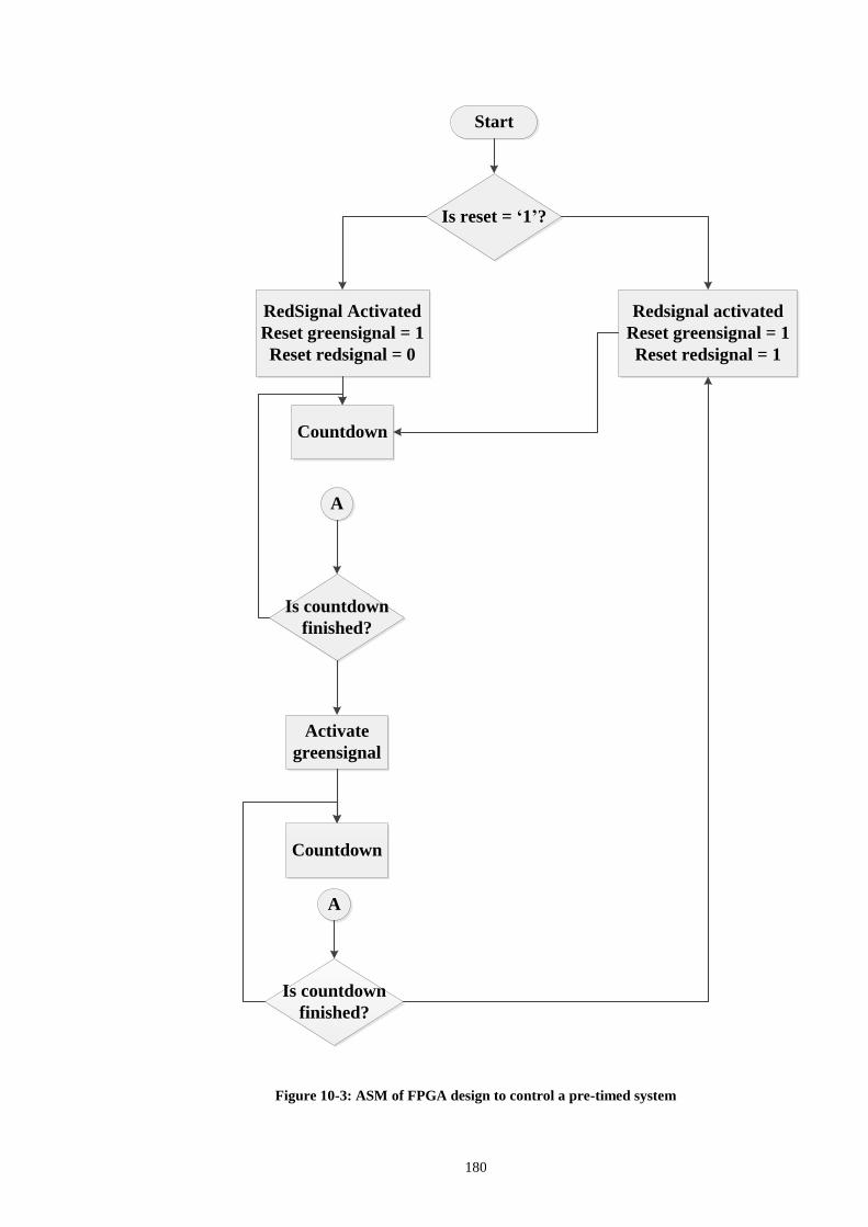
180
Start
Is reset = ‘1’?
RedSignal Activated
Reset greensignal = 1
Reset redsignal = 0
Countdown
A
Is countdown
finished?
Activate
greensignal
Countdown
A
Is countdown
finished?
Redsignal activated
Reset greensignal = 1
Reset redsignal = 1
Figure 10-3: ASM of FPGA design to control a pre-timed system

181
Countdown
Is reset = ‘1’?
Is Code =
‘0000'
?
Donesignal = 0
Donesignal = 1
A
YES NO
YES
NO
Figure 10-4: Countdown procedure in an FPGA design to control a pre-timed system
The VHDL program that describes the above ASM should consist of a set of nested if
conditions, together with a counter used to carry out the countdown process of the
traffic signal. The hardware controller constantly compares the optimized traffic signal
timings, which is hardwired into the design, with the current counter timing and decides
whether to stay in the current state or to pass onto the next state.
The design defines a set of signals to be used throughout the coding. However, two
signals are the most critical to the operation of the design. These are redsignal (R1) and
greensignal (G1). R1 signifies the red signalization state for control point 1 in the
intersection in study, while G1 represents the green signalization to control point 1. R1,
being the red signal for control point1, is definitely being a green signal for the opposite

182
control point 2, as the intersection on which the design is implemented is a simple two-
way intersection.
Table 10-2: design signals correspondent to signal timings in FPGA design
Control Point Signalization State timing Design signal
1 R G “R1”
2 G R “G1”
These two signals have a value of either “0” or “1” depending on the logical structure of
the coding.
Two other signals, which are not less important than the first two, are also defined in the
design. These are “resetsignalgreen” and “resetsignalred”. They indicate the
initialization of the state timings.
The major procedure in the design is the timing control process, where the state
transition takes place. It consists of a set of nested if conditions that describe the logical
sequence of the state machine illustrated above.
The “if then else” conditions start with checking the reset button. The reset button is an
input button assigned on the FPGA to manually reset the two signals whenever desired.
If reset button is pushed, both signal timings are initialized through pulsing ones to both
the reset signals. Then, the program is designed to activate the redsignal “R1” as
default. Countdown of R1 starts, with the entered value of the previously optimized
state timing. Countdown is another procedure, which counts down the signal timings.
Whenever the countdown is ended, a signal called “donesignal” is pulsed.
Once R1 is activated and the countdown starts, state R1 is the dominant state, while the
green state timing is still fixed and not shown on the display. As soon as the countdown
process ends, the state transition takes place, G1 signal dominates, and the countdown is
now assigned to the green signal. At last, when the green state timing tends to zero, after

183
the countdown process, both signals are reset, the red signal R1 is activated once again,
marking the start of a new cycle.
The state timings’ countdown is displayed as output signals on 7-segments for
visualization. In real world application, the signal light displays will replace the 7-
segments.
10.4 FPGA SYNTHESIS AND IMPLEMENTATION
The design has been written out in VHDL language in the Xilinx ISE environment. The
Xilinx XST tool has synthesized the design into hardware components as shown in
figure 10-5.

184
Figure 10-5: Design Synthesis
The synthesized design is then placed and routed using the Xilinx Place & Route tool. A
screen snapshot of the design placed on the FPGA is given in figure 10-6.

185
Figure 10-6: Routing and placing
10.5 PROTOTYPING
Now that the FPGA design is successfully running, it is strongly recommended to
model the work on a physical prototype to ensure the reliability of the program design,
and visualize the work done.
The prototype consisted of two opposite wooden plates representing the main two
vehicular streams. Adequate landscape, road layout, aesthetic features are carefully
design to physically approach the reality. Each wooden plate is driven by a DC motor.
Once the prototype is accurately installed, the program is started. The FPGA
implements the logical pre-designed sequence.
As “R1” is activated, two signals are generated. One signal is sent to the DC Motor 2
“M2” connected to the correspondent control point (CP2). The motor catches the signal;
motion is generated and transmitted to the wooden plate representing the control point
having the green signalization. The motion of the wooden plate, with vehicles attached
on its interface, represents the dissipation of vehicular flow in CP (2) and the queuing
process in CP (1). The other signal is sent to the 7 segment which display the
correspondent pre-optimized state timing.

186
FPGA
controller
O/P signal 1
O/P signal 2
Inputs
DC Motor 1
DC Motor 2
7 segment
display A
7 segment
display B
O/P signal 1'
O/P signal 2'
Control Point
1
Control Point
2
Figure 10-7: Theory of operation of the prototype of FPGA controlling a traffic system
As soon as the countdown finishes, the FPGA design is followed to carry out the state
transition process. Similar signals are sent to DC Motor 1 and the correspondent 7-
segment to represent the opposite state. And hence, the cycle is pursued representing a
simplified prototype of a pre-timed traffic control system fully controlled by FPGA’s.

187
Figure 10-8: The prototype representing FPGA control in a pre-timed traffic control system
10.6 CONCLUSIONS
Through experimentation, FPGA control, a modern trend in the world of control and
automation, has proven its reliability and success in the field of traffic control. Based on
the experimentation results attained in this chapter, FPGA’s can be successfully
implemented to control the operation of a pre-timed traffic control system. It ensures the
complete automation of the system, without the need of any human interference.

188
C h a p t e r e l e v e n
11 FPGA CONTROL IN AN ADAPTIVE TRAFFIC
SYSTEM
11.1 INTRODUCTION TO FPGA’S
Short for Field-Programmable Gate Array, a type of logic chip that can be programmed.
Field Programmable refers that the FPGA's function is defined by a user's program
rather than by the manufacturer of the device.
The main difference between FPGA’s and IC’s is that a typical integrated circuit
performs a particular function defined at the time of manufacture. In contrast, the
FPGA's function is defined by a program written by someone other than the device
manufacturer. This user programmability gives the user access to complex integrated
designs without the high engineering costs associated with application specific
integrated circuits.
Top 5 Benefits of FPGA Technology
Performance
User programmability
Cost
Operation
Performance: FPGA’s highly exceed the traditional performance of controllers and
processors.
User programmability: The FPGA design can be altered at any time to reflect desired
changes in the model.
Cost: FPGA’s are not relatively expensive compared to the sophisticated devices used
in traffic control in most developed countries.

189
Operation: FPGA’s are user friendly, they are easy to design and program. In addition,
once programmed, they can easily operate the traffic control network without
interruption or breakdowns.
11.2 THE DESIGN OF A FPGA-BASED ADAPTIVE TRAFFIC
CONTROL SYSTEM: THEORY OF OPERATION
In the previous chapter, FPGA control has proven its efficiency as a reliable strategy to
control the operation of a pre-timed traffic control systems.
This section of the report throws up a question to whether FPGA control can be used to
control an adaptive traffic control system.
Adaptive traffic control systems are quite different than pre-timed systems. In these
systems, signal timings change constantly from one cycle to another based on the
current state of the intersection. This state is often determined using modern sensing
devices.
Achieving an FPGA design for that type of system is thought to be a complex operation.
However, the concept of the design can easily be understood.
Most modern FPGA’s have input ports for surveillance cameras and other counting
devices. If these devices can be –by any means- connected to the sensing devices that
determine the current system state, FPGA’s could certainly sense the traffic
environment.
An FPGA program design can be developed to process this signal into timings. This can
be done through a simple equation which calculates the timings necessary to dissipate a
given queue length based on the dissipation rates characterizing each control point.
Finally the FPGA should be directly connected to the traffic lights for the output
numbers to be shown on the control points’ displays.

190
11.3 FPGA’S: ADVANTAGES VS. LIMITATIONS
FPGA design tools are increasingly available, allowing control system designers to
more quickly create and adapt FPGA hardware. It is expected in the future, that FPGA’s
will replace the traditional controllers in most systems.
However, there exist some limitations to the use of FPGA’s in traffic control systems:
Completely automating the traffic environment will increase the installation and
maintenance costs compared to traditional traffic control systems.
Increasing the amount of hardware devices in a system, will definitely increase
the chances of failures. Therefore, adequate maintenance plan should be carried
out to overcome this problem and preserve the reliability of the system.
FPGA’s should be placed in a well-protected control unit for the purpose of
protection from climate changes, theft or any damage. High protection should be
provided because a single error in the FPGA structure will definitely lead to the
failure of the control system and the dominance of chaos in the surrounding
environment.
11.4 CONCLUSIONS
The modern ways of traffic management improves the traffic condition up to a large
extent. Advanced signalling controllers contribute to the improvement of the urban
traffic. FPGA control is a proposed control strategy to automate the traffic control
environment and hence, lead to a better system performance.

191
C h a p t e r t w e l v e
12 CONCLUSIONS AND RECOMMENDATIONS
This project has shed light on one of the vital problems that threaten the splendour of
the beautiful city of Alexandria, and the livelihood of its citizens. The problem of traffic
congestion has become a heavy burden on the shoulders of both the governments and
the peoples. The absence of a reliable control strategy that regulates the traffic control
operation is one of the main motives of this problem. Throughout the course of this
report, various techniques and approaches have been suggested to overcome the traffic
congestion dilemma and cut off the problem from its root causes.
Through careful field observation and problem monitoring, data about the system
variables, parameters and metrics through different periods of the day, has been
collected in order to define the underlying aspects of the problem. Adequate statistical
analysis has been carried out for data treatment, fitting and analysis. This has been a
crucial phase of the project, as the accuracy of the collected data has been the strong
base which held all the work done together.
In addition, an analytical model formulation has been developed to accurately represent
the system. The model clearly defines the decision and response variables, the system
parameters, the proposed objective function(s) and the governing constraints. Several
solution approaches have been proposed to solve the formulated model.
Genetic Algorithm, a computational approach inspired by the evolution theory, and a
revolution in the world of meta-heuristic techniques, is a powerful optimization tool that
shows itself as a reliable solution. A successful Genetic Algorithm experiment has been
conducted for the purpose of optimizing traffic signal timings in two consecutive
intersections in Alexandria’s road network. The G.A. optimized signal timings have
been entered to a developed simulation model to emulate the consequences that might
take place. Promising results have been obtained, indicating great improvements in the
performance of the system. Compared to the actual system performance, general
average queue length has reduced by 43 %, while the general average vehicular waiting
time showed a similar decrease of 30.2 %.

192
Turning to a completely new approach to handle the problem, simulation has been
suggested as a reliable solution. Extendsim8, a powerful simulation package has been
successfully utilized to develop a simulation model that accurately replicates the system
under study. The actual performance of the current situation, under the current
circumstances, has been simulated. It has been demonstrated that the current state of the
system exhibits relatively weak performance, due to the extreme values of queue
lengths and vehicular waiting times that have been detected. Moreover, simulation has
been utilized to develop better scenarios for the system. Scenario1, a proposed
simulation model for the system, through making a major change in the road network’s
phase plan and operational logic, has been suggested and proven to exhibit remarkable
improvement in terms of performance metrics. General average queue length has
decreased by 4 %, while the average vehicular waiting time has been reduced by 29.6
%.
In addition, Optimization using simulation has arisen as one of the main solution
techniques of this project. Using Extendsim8 optimizer, the set of signal timings
controlling the road network under study has been optimized and simulated. Favorable
results have been attained, signifying the success of the optimization experiments. The
general average queue length has decreased by 11.3 %, while the general vehicular
waiting time has reduced by 17%.
All The previous proposed solutions have been planned to analyze and control the
performance of a pre-timed traffic control system. Adaptive, also called smart or
actuated, traffic control systems represent the most advance phase of traffic strategies.
ATCSs’ adapt their signal timings instantaneously according to the current demand
pattern. A simulation model has been developed to study the possibility of applying an
adaptive traffic control system to a simple two way intersection in Alexandria, Egypt.
The results showed the greatest improvement, as ATCS’s are well-known in the
developed countries of their superiority over the traditional pre-timed systems. General
queue length has decreased by 74%, whereas vehicular waiting time has been reduced
by 69.2 %.
Holding comparisons between different proposed solutions, along with the actual
performance is one of the major conclusions of this project. Charts shown in Figures

193
12-1, 12-2, 12-3 and 12-4 visualize these comparisons and help the decision makers in
deciding which strategy to implement.
Figure 12-1: Actual system vs. all the proposed solutions in terms of LQav
Figure 12-2: Actual system vs. all the proposed solutions in terms of WQav
0
5
10
15
20
25
30
1 2 3 4 5
Avg
. LQ
Periods
Actual VS. ALL Solutions
Actual
Scenario 1
GA
Optimized scenario 1
0
5
10
15
20
25
30
35
40
1 2 3 4 5
Avg
. MQ
Periods
Actual VS. ALL Solutions
Actual
Scenario 1
GA
Optimized Scenario 1

194
Figure 12-3: Actual vs. all proposed solutions in terms of (LQav * WQav)
Figure 12-4: Actual system vs. adaptive model in terms of (LQav*WQav)
The last part of the report has covered a deep introduction to the technological
advancements in the hardware used in traffic control. Traffic control using FPGA’s,
the latest trend in the world of automation and control, has appeared to be a reliable
control strategy. The possibility of applying FPGA control to a pre-timed traffic control
system has been studied, and proven to be successfully operating. The optimized
timings have been entered in the FPGA design, which achieves the automatic state
transition and control over the road network. This is expected to be a large step forward
0
200
400
600
800
1000
1200
1400
1600
1800
1 2 3 4 5
Avg
. LQ
*MQ
Periods
Actual VS. All Solutions
Actual
Scenario 1
GA
Optmized Scenario 1
0
50
100
150
200
250
1 2 3 4 5
Avg
. LQ
*MQ
Periods
Actual VS. Adaptive
Actual
Adaptive

195
towards the automation of traffic control systems, minimizing human interference as
much as possible.
Recommendations
The greatest evaluation challenge for this project is to be implemented on the real-world
system. It would be interesting to experiment the attained results on the steady ground
of reality and assess the consequences that may take place.
It is also remarkable that, unless both the government and the citizens cooperate through
awareness and efforts, tangible improvements to the traffic environment can hardly be
created.
In case of the success of the implementation phase, the study could be generalized to
other major intersections in Alexandria’s road network to cut off one of the major
problems that threatens the stability and the splendour of this beautiful city.
196
REFERENCES
[1] R. P. Roess, E. S. Prassas, and W. R. McShane, Traffic Engineering: Pearson, 2011.
[2] L. Vas, "Mathematical Modeling - Introduction and early examples."
[3] "Introduction to Analytical problem solving."
[4] G. V.Caliri, "Introduction to Analytical Modeling," U.S.A.
[5] T. V. Mathew, "Genetic Algorithm," Indian institute of technology, Bombay, India.
[6] E. K. Prebys, "The Genetic Algorithm in Computer Science," MIT Undergraduate Journal of
Mathematics, pp. 165-170.
[7] P. Reed, B. Minsker, and D. E.Goldberg, "Design a competent simple genetic algorithm for
search and optimization," 2000.
[8] R. P. Roess, E. S. Prassas, and W. R. McShane, Traffic Engineering, Fourth edition ed.: Pearson.
[9] K. Saharia, "Traffic Optimization System: Using a Heuristic Algorithm to Optimize
Traffic Flow and Reduce Net Energy Consumption," Monta Vista High School
USA.
[10] J.-Q. Li, G. Wub, and N. Zou, "Investigation of the impacts of signal timing on vehicle
emissions
at an isolated intersection," Transportation Research Part D 16 (2011) 409–414, vol. 16, pp. 409–414,
2011.
[11] X. Li, G. Li, S.-S. Pang, X. Yang, and J. Tian, "Signal timing of intersections using integrated
optimization
of traffic quality, emissions and fuel consumption: a note," Transportation Research Part D vol. 9, pp.
401-407, 2004.
[12] M. Dotoli, M. P. Fanti, and C. Meloni, "A signal timing plan formulation for urban traffic
control," Control Engineering Practice
vol. 14, pp. 1297–1311, 2006.
[13] A. Azadeh and A. Sadeghnia, "Design and Optimization of a Traffic Control System by
Integration of Computer Simulation and Genetic Algorithm," Australian Journal of Basic and
Applied Sciences, vol. 3, pp. 4333-4343, 2009.
[14] T. Kalganova, G.Russell, and A. Cumming, "Multiple Traffic Signal Control Using A Genetic
Algorithm," presented at the Fourth International conference on artificial neural networks and
genetic algorithms, Portoroz, Slovenia, 1999.
[15] L. Singh, S. Tripathi, and H. Arora, "Time Optimization for Traffic Signal Control
Using Genetic Algorithm," International Journal of Recent Trends in Engineering, vol. 2, pp. 4-6, 2009.
[16] L. Zang, P. Hu, and W. Zhu, "Study on Dynamic Coordinated Control of Traffic Signals
for Oversaturated Arterials " Journal of Information & Computational Science vol. 9, pp. 3625–3632,
2012.
[17] Y. K. Chin, K. C. Yong, N. Bolong, S. S. Yang, and K. T. K. Teo, "Multiple Intersections
Traffic Signal Timing
Optimization with Genetic Algorithm," presented at the International Conference on Control System,
Computing and Engineering, 2011.

197
[18] J. He and Z. Hou, "Ant colony algorithm for traffic signal timing optimization
" Advances in Engineering Software vol. 43, pp. 14-18, 2012.
[19] R. Putha, L. Quadrifoglio, and E. Zechman, "Comparing Ant Colony Optimization and Genetic
Algorithm Approaches for Solving Traffic Signal
Coordination under Oversaturation Conditions," Computer-Aided Civil and Infrastructure Engineering
pp. 14-28, 2012.
[20] R. G. Ingalls, "Introduction to simulation," presented at the Winter simulation conference, 2011.
[21] A. M. Law, "How to build valid and credible simulation models " presented at the Winter
simulation conference, 2009.
[22] R. E. Shannon, "Introduction to the art and schience of simulation " presented at the Winter
simulation conference, 1998.
[23] J. Banks, "Introduction to simulation," presented at the Winter simulation conference, 2000.
[24] R. G. Ingalls, "Introduction to simulation," presented at the Winter simulation conference, 2001.
[25] A. M. Law, "How to conduct a successful simulation study " presented at the Winter simulation
conference, 2003.
[26] J. Banks, J. S. C. II, B. L. Nelson, and D. M. Nicol, Discrete-Event System Simulation, Fifth
Edition ed.: Prentice Hall, 2009.
[27] A. M.Law, Simulation Modeling and analysis, 4th edition ed. USA: Prentice Hall, 2006.
[28] M. Pidd, Computer simulation in management science, 3rd edition ed., 1992.
[29] W. D. Kelton, R. P. Sadowski, D. T. Sturrock, W. Kelton, R. Sadowski, and D. Sturrock,
Simulation with Arena, 4th edition ed.: McGraw-Hill Science, 2003.
[30] L. G. Birta and G. Arbez, Modelling and Simulation: Exploring Dynamic System Behaviour,
2007 edition (January 24, 2011) ed., 2011.
[31] D. C. Harrell, Dr.Biman, K.Ghosh, and D. R. O.Bowden, Simulation using Promodel, Second
edition ed.
[32] B. Sadoun. (2008) On the Simulation of Traffic Signals Operation 285-295.
[33] C. M. Mwangi, S. M. Kang’ethe, and G. N. Nyakoe, "Design and simulation of a fuzzy logic
traffic signal controller for a signalized intersection " presented at the JKUAT scientific
technological and industrialization conference, Kenya, 2010.
[34] R. H. Smith and D. C. Chin, "Evaluation of an Adaptive Traffic Control Technique with
Underlying System Changes," presented at the Winter Simulation Conference, 1995.
[35] J. Clark and G. Daigle, "The importance of simulation techniques in its research and analysis,"
presented at the Winter simulation conference, 1997.
[36] M. STANIEK, "The cross roads lights fuzzy controller development principles in VISSIM
environment," ZESZYTY NAUKOWE POLITECHNIKI SLASKIEJ, pp. 88-95, 2011.
[37] A. Albagul, M. Hrairi, Wahyudi, and M. F. Hidayathullah, "Design and Development of Sensor
Based Traffic Light System," American Journal of Applied Sciences vol. 3, pp. 1745-1749,
2006.

198
[38] M. E. Fouladvand, Z. Sadjadi, and M. R. Shaebani, "Optimized traffic flow at a single
intersection: traffic responsive signalization," JOURNAL OF PHYSICS A: MATHEMATICAL
AND GENERAL, pp. 561-579, 2004.
[39] D.-W. Huang and W.-N. Huang, "Optimization of Traffic lights at crossroads," International
Journal of Modern Physics C, vol. 14, pp. 539-548, 2003.
[40] S. Belbasi and M. E. Foulaadvand, "Simulation of traffic flow at a signalized Intersection,"
Journal of Statistical Mechanics: Theory and Experiment, pp. 1-15, 2008.
[41] K. Yamada and T. N.Lam, "Simulation Analysis of two adjacent traffic signals," presented at the
Winter simulation conference, 1985.
[42] E. C. P. Chang, "How to decide the interconnection of isolated traffic signals," presented at the
Winter simulation conference, 1985.
[43] S.-B. Cools, C. Gershenson, and B. D’Hooghe, "Self-organizing traffic lights: A realistic
simulation," 2006.
[44] P. Li and M. Abbas, "Stochastic Dilemma Hazard Model at High-Speed Signalized
Intersections," Journal of transportation and engineering, vol. 136, pp. 448-456, 2010.
[45] K. N. Hewage and J. Y. Ruwanpura, "Optimization of traffic signal light timing using
simulation," presented at the Winter simulation conference, 2004.
[46] W. C. Howell and M. C. Fu, "Simulation Optimization of Traffic Light Signal Timings via
Perturbation Analysis," 2006.
[47] A. A.Saka, G. Anandalingham, and N. J.Garber, "Traffic signal timing at isolated intersections
using simulation optimization," presented at the Winter simulation conference, 1986.
[48] J. J.Swayn. (2009) To Boldly Go. ORMS. 50-53.
[49] "Recent Modeling Enhacement to CORSIM," ed: University of Florida,Transportation Research
Center and theMcTrans Center, 2012.
[50] I. ITT Industries, Systems Division and A. R. D. a. S. E. P. Team, "CORSIM User's Guide," ed,
2006.
[51] L. E. Owen, Y. Zhang, L. Rao, and G. McHale, "Traffic flow simulation using CORSIM,"
presented at the Winter Simulation Conference 2000.
[52] B. Diamond, D. Krahl, A. Nastasi, and P. Tag, "Extendsim advanced technology: integrated
simulation database," presented at the Winter simulation conference, 2010.
[53] D. Krahl, "Extend: an interactive simulation tool," presented at the Winter simulation
conference, 2003.
[54] D. Krahl, "Extendsim 7," presented at the Winter simulation conference, 2008.
[55] G. S. a. partners, "Traffic data collection procedures ", Kentucky, USA2002.
[56] m. o. w. a. t. Roads department, Botswana, "Traffic data collection and analysis," 2004.
[57] R. T.Hintersteiner, "Vehicle detectors."
[58] D. D. Romero, A. S. Prabuwono, Taufik, and A. Hasniaty, "A review of sensing techniques for
real time traffic surveillance," Journal of applied sciences vol. 11, pp. 192-198, 2011.

199
[59] M. Gentili and P. B. Mirchandani, "Locating sensors on traffic networks: Models, challenges and
research opportunities
" Transportation Research Part C vol. 24, 2012.
[60] M. Gentili and P. B. Mirchandani, "Locating Active Sensors on Traffic Network," Springer
Science,Annals of Operations Research vol. 136, pp. 229-257, 2005.
[61] R.Weil, J.Wootton, and A.Gurcia-Ortiz, "Traffic incident detection:sensors and algorithms,"
Elsevier science Ltd ,Mathl Comput. Modelling, vol. 27, pp. 257-291, 1998.
[62] Extendsim8 user guide

200
APPENDICES
Appendix (A): Genetic Algorithm coding using VBA.
Appendix (B): Extendsim8 blocks and libraries.
Appendix (C): Data points and observations.

201
APPENDIX (A): GA CODING USING VBA

202

203
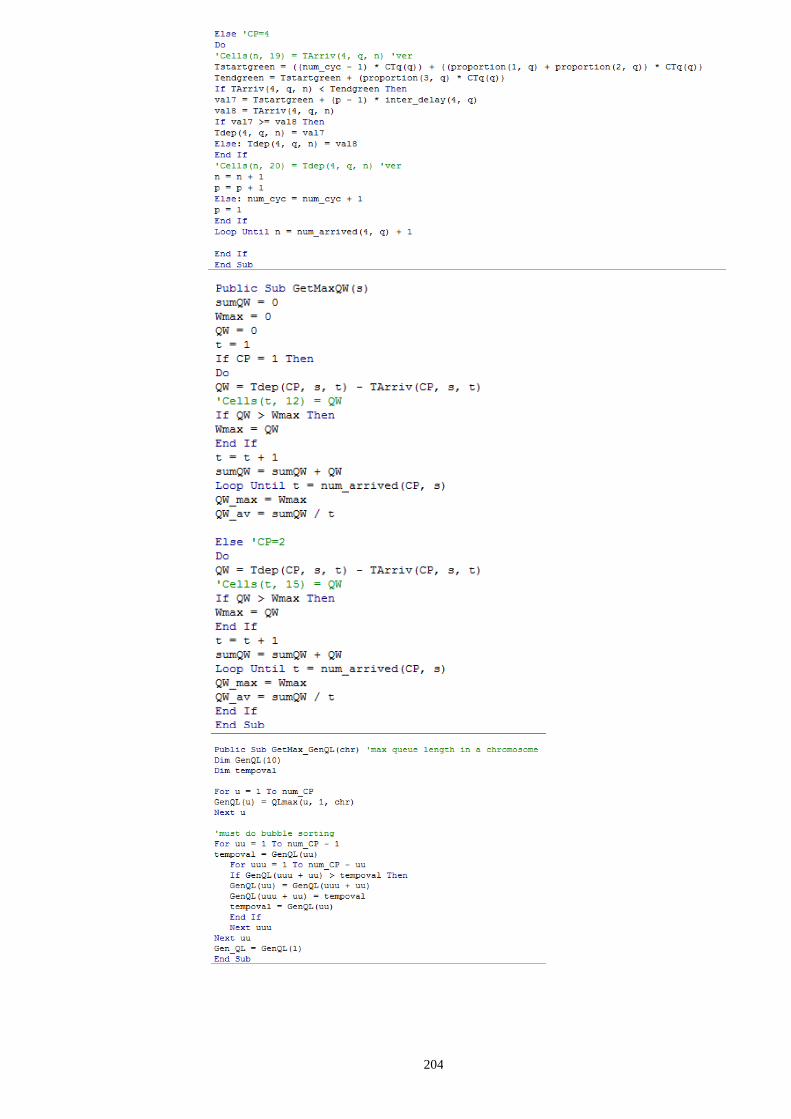
204

205

206
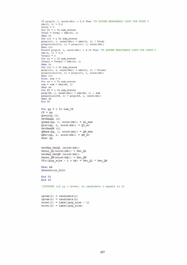
207

208

209
APPENDIX (B): EXTENDSIM8 BLOCKS AND
LIBRARIES
Block Function
Lookup
Table
Acts as a lookup table (x in and y out) that are used to calculate what the output
value would be for the given input. Input values can come from an input
connector (the default) or can be simulation time. The output can be discrete,
interpolated or stepped.
Optimizer
Searches for the best set of model parameters that maximizes profit or
minimizes cost, given parameter limits and any entered constraints. Uses
evolutionary strategies that are similar to genetic algorithms.
Mean &
Variance
Calculates the mean, variance, and standard deviation of the values input during
the simulation.
Information
Reports statistics about the items that pass through it, such as cycle time and
TBI (Time Between Items).
Equation(I)
Calculates equations when an item passes through. The equations can use
multiple inputs and properties of the item as variables, and the result(s) of the
equations can be assigned to multiple outputs and properties of the item.
Queue
Queues items and releases them based on a user selected queuing algorithm,
such as Resource pool queue, Attribute value, First in first out, Last in first out,
and Priority. Options include reneging and setting wait time. If you need more
advanced control over the queuing algorithm, consider using the Queue
Equation block, below.
Create
Provides items or values for a discrete event simulation at specified interarrival
times. Choose either a distribution or a schedule for the arrival of items or
values into the model.
Exit
Passes items out of the simulation. The total number of items absorbed by this
block is reported in its dialog and at the value output connectors.

210
Block Function
Gate
Limits the passing of items through a portion of the model, either by demand or
by using a sensor connector to monitor how many items are in a section of the
model.
Select Item
In
Selects items from one input to be output based on a decision.
Select Item
Out
Selects which output gets items from the input, based on a decision
Executive
This block must be placed to the left of all other blocks in discrete event and
discrete rate models. It does event scheduling and provides for simulation
control, item allocation, attribute management, and other discrete event and
discrete rate model settings.
Decision
Makes a decision and outputs TRUE or FALSE values based on the inputs and
defined logic. The dialog lets you perform the following tests comparing A to
B: greater than, greater than or equal to, equal to, less than, less than or equal
to, and not equal. You can also test for A being an invalid number (noValue).
The block can be set to use hysteresis.
Equation
Outputs the results of the equations entered in the dialog. You can use
ExtendSim's built-in operators, functions, and some or all of the input values as
part of the equation. The equations can have any number of inputs and any
number of outputs.
Max & Min
Determines the maximum and minimum values from among the values input.
The dialog shows the maximum and minimum values and the input connectors
they came from. The block outputs the maximum or minimum values and the
respective connector number.

211
APPENDIX (C): DATA COLLECTION POINTS AND
OBSERVATIONS
Inter-arrivals for 7-9 am
intersection 1 intersection 2
1' 2' 1 2 3 4
A D A D A D A D D
0 0 0 0 0.26 0.26 47.68 0 0 0 0
49.51 1.79 0.25 1.8 0.28 0.28 0.99 13.17 2.07 11.03 8.6
1.95 4.41 2.17 2.05 0.31 0.31 0.9 2.17 6.76 1.57 1.96
2.92 4.37 0.95 2.64 0.32 0.32 1.21 1.95 1.92 1.37 4.02
4.85 5.33 2.99 2.26 0.34 0.34 0.84 7.57 26.43 4.83 8.15
5.73 17.81 1.03 1.93 0.34 0.34 1.85 3.97 0.84 25.95 6.43
2.37 2.32 1.22 1.33 0.34 0.34 0.58 3.62 1.24 1.56 10.57
6.87 4.67 1.09 2.79 0.35 0.35 2.39 0.91 72.47 1.19 5.57
15.43 3.22 0.99 7.95 0.37 0.37 2.12 2.64 3.15 2.62 0.55
3.03 4.06 4.34 9.86 0.37 0.37 0.59 4.84 1.62 1.02 75.73
0.92 3.06 2.37 2.75 0.38 0.38 1.81 4.54 3.67 0.24 3.83
5.13 64.25 10.44 0.24 0.39 0.39 1.53 3.47 0.59 79 6.61
2.44 2.25 43.31 1.89 0.39 0.39 1.22 5.3 5.57 4.79 3.09
5.04 3.53 0.26 1.27 0.4 0.4 4.46 2.36 5 0.74 13.99
3.67 3.04 1.26 1.41 0.41 0.41 1.19 5.62 1.11 1.08 3.41
32 3.01 0.91 0.5 0.41 0.41 1.68 1.57 2 0.72 8.53
30.5 2.63 2.03 0.53 0.42 0.42 2.34 2.41 6.97 2.36 5.59
1.76 4.65 1.06 0.73 0.42 0.42 1.57 0.71 95.76 8.3 3.93
1.13 2.28 1.23 0.81 0.43 0.43 0.99 0.97 1.75 7.13 66.47
1.4 1.75 0.24 0.89 0.45 0.45 0.92 2.54 1.52 6.67 16.41
4.31 6.36 2.26 1.73 0.46 0.46 2 1.53 1.04 1.25 11.04
2.13 2.53 1.09 0.56 0.46 0.46 2.08 0.76 5.84 6.07 3.29
1.66 0.35 1.74 0.79 0.46 0.46 0.53 1.54 2.43 3.83 5.98
1.24 1.3 3.52 2.95 0.47 0.47 1.18 1.17 2.83 1.45 5.75
4.32 2.26 0.79 4.3 0.48 0.48 0.59 1.62 2.61 5.79 3.16
1.27 1.25 0.52 2.53 0.5 0.5 0.65 4.14 1.36 1.45 3.84
3.86 2.23 3.11 1.81 0.51 0.51 0.69 0.73 2.24 1.64 1.14
1.04 2.07 1.16 58.13 0.52 0.52 3.01 2.13 2.93 71.7 2.54
5.4 1.54 2.72 6.75 0.53 0.53 1.21 2.51 35.95 4.54 0.55
0.31 2.93 2.15 3.24 0.53 0.53 2.51 1.15 81.88 7.71 6.88
2.39 1.07 0.51 8.83 0.53 0.53 1.39 1.4 0.47 12.45 59.28
1.59 53.42 2.23 3.3 0.54 0.54 4.19 5.66 0.7 12.34 5.25
1.54 2.57 6.42 1.01 0.55 0.55 1.49 3.93 1.59 2.75 6.76

212
Inter-arrivals for 9-1 pm
intersection 1 intersection 2
1' 2' 1 2 3 4
A D A D A D A D D
0 0 0 0 0 0 0 0 0 0 1.09
20.18 0.82 6.15 3.06 2.15 62.74 1.77 0.56 5.41 1.12 2.37
1.77 1.24 2.71 5.87 1.65 6.37 0.93 2.24 1.47 1.29 4.67
12.11 0.89 2.15 2.21 2.44 4.25 1.19 8.55 3.63 1.93 2.23
4.6 1.29 4.37 6.36 5.55 1.53 0.48 1.3 20.63 1.55 5.92
5.1 2.84 0.39 3.83 1.98 1.38 0.46 1.02 87.58 1.66 2.63
7.67 1.38 1.72 7.59 1.38 17.45 0.5 1.04 3.59 5.45 2.59
11.37 1.56 3.02 76.69 3.72 25.34 0.53 1.93 2.1 3.18 72.19
4.6 1.53 1.33 1.52 8.41 13.43 0.58 4.39 2.1 6.36 7.72
1.18 1.68 9.51 3.45 18.01 13.06 1.3 31.54 2.28 2.58 4.21
0.87 3.06 1.8 20.87 15.28 2.42 0.44 1.7 15.81 10.33 3.19
7.05 1.94 27.13 6.8 13.22 4.47 1.35 3.45 2.07 2.41 7.08
4.58 6.69 13.47 2.74 1.2 5.31 0.38 2.65 1.82 4.9 2.84
13.53 10.43 0.33 81.12 1.2 7.3 0.65 1.37 9.19 1.21 4.96
3.9 14.84 0.38 1.55 2.05 2.29 1.33 2.27 80.33 6.58 10.46
4.43 55.37 3.55 4.44 2.32 2.6 0.56 0.29 1.74 79.35 0.72
4.75 1.08 0.44 36.78 0.22 5.43 1.67 0.92 6.78 1.35 1.6
2.02 4.48 4.79 17.24 1.48 41.88 0.44 0.76 4.58 0.96 1.43
3.59 3.44 1.61 1.29 0.71 2.73 1.72 1.74 30.66 4.53 82.21
2.94 3.57 0.92 0.82 0.79 21.6 4.29 1.04 1.6 4.06 1.85
11.2 3.55 0.77 0.81 6.19 19.62 1.61 1.61 1.99 1.91 1.4
4.89 7.23 1.74 0.46 1.14 1.74 0.48 6.34 1.4 2.96 2.05
2.54 15.22 0.99 0.25 3.33 3.28 1.28 1.97 1.81 2.46 6.68
1.87 3.91 0.45 0.57 2.44 3.52 0.72 1.26 2.33 4.74 9.03
3.62 0.64 5.77 0.4 7.3 25.26 1.86 1.45 0.87 1.87 6.69
1.44 0.97 2.18 0.25 0.86 2.95 0.63 1.06 6.52 0.85 4.47
5.31 4.07 2.95 1.03 3.08 1.65 1.01 1.76 2.2 2.51 47.81
3.25 3.69 1.5 0.63 5.83 3.23 0.6 0.49 1.89 5.41 1.62
3.41 60.09 0.87 1.9 1.06 1.61 2.45 1.44 2.56 40.86 4.79
2.29 2.12 1.07 0.37 1.16 4.3 1.66 4.11 2.97 34.19 1.67
1.11 1.35 0.73 0.98 3.15 5.25 2.65 7.24 0.57 0.39 17.01
5.46 1.03 4.95 1.83 5.85 1.51 9.66 34.36 0.48 2.22 3.3
8.11 0.99 2.45 0.89 1.39 2.3 2.11 7.61 2.05 1.83 8.39

213
Inter-arrivals for 1- 5 pm
intersection 1 intersection 2
1' 2' 1 2 3 4
A D A D A D A D D
2.16 2.15 0.65 1.9 4.13 0.14 4.71 0.88 1.16 22.75 2.79
0.47 0.55 0.52 2.91 2.54 0.18 3.5 3.06 1.51 5.28 2.37
1.03 2.96 0.5 5.51 0.54 0.19 0.41 5.54 5.4 5.22 5.38
2.85 0.45 1.45 2.35 7.48 0.2 7.5 2.92 2.18 0.98 1.92
1.13 0.43 1.85 2.32 1 0.21 0.81 9.92 61.13 32.75 1.4
0.59 3.98 0.69 2.06 28.86 0.21 0.37 1.49 1.33 3.91 2.6
1.46 0.55 0.98 1.69 5.75 0.22 1.79 4.57 0.83 20.89 29.01
1.85 2.49 2.11 0.82 3.49 0.22 0.64 3.44 1.02 1.12 2.38
2.04 0.75 0.68 1.3 2.52 0.23 0.94 14.6 1.39 1.22 2.41
4.46 2.14 0.47 0.74 1.97 0.23 2.19 2.8 1.34 2.73 4.09
1.1 0.81 1.97 1.57 11.56 0.24 1.35 18.3 2.41 1.84 2.09
2.37 5.64 0.81 0.86 1.66 0.24 0.76 3.66 12.25 2.37 2.57
0.84 0.81 0.87 0.83 1.84 0.24 0.34 1.98 1.9 1.88 6.96
12.38 2.22 0.55 1.09 19.69 0.24 2.83 9.62 19.87 93.26 5.74
0.84 1.5 4.49 0.92 0.93 0.25 2.94 2.31 4.49 6.17 5.31
0.61 60.77 2.51 0.95 2.55 0.27 0.54 1.93 5.35 2.34 3.59
4.64 0.97 4.95 0.78 4.51 0.28 1.44 1.19 0.93 4.79 90.9
1.14 1.22 5.66 0.69 1.99 0.28 1 3.62 1.08 1.49 2.02
3.69 2.43 0.55 0.65 1.24 0.29 0.32 1.99 2.64 1.42 0.56
0.54 0.37 0.52 0.5 19.63 0.3 3.24 2.51 1.56 87.97 19.57
0.67 3.14 2.46 0.78 9.63 0.3 0.41 5.53 1.01 6.47 1.41
0.8 1.43 2.57 0.5 3.9 0.33 1.31 2.24 4.21 8.84 1.52
0.67 12.16 1.4 0.41 18.55 0.34 0.91 3.52 8.89 6.27 5.2
1.37 0.25 2.1 1.09 2.62 0.34 0.78 0.61 1.05 2.8 1.34
1.06 0.68 0.82 0.63 1.31 0.34 2.45 14.19 1.3 1.49 0.58
1.44 0.27 0.49 0.57 3.11 0.35 1.14 4.34 1.91 2.7 1.87
2.36 1.15 1.77 0.72 3.74 0.35 2.26 6.66 60.06 7.57 1.42
0.72 2.32 4.71 2.4 2.19 0.36 0.34 1.31 1.3 2.7 81.22
5.7 4.88 8.52 0.92 2.37 0.37 0.42 2.13 1.98 3.52 3.55
1.44 0.25 13.9 0.73 4.82 0.37 2.17 4.43 1.17 12.76 0.88
2.71 0.36 1.51 25.44 4.39 0.38 1.31 0.82 1.51 7.36 1.78
8.75 1.64 20.8 30.41 9.12 0.39 0.31 5.74 1.03 1.42 1.54
1.17 1.63 2.96 0.82 0.85 0.4 52.78 9.27 1.08 14.96 1.62
6.38 0.3 1.3 0.53 1.07 0.41 9.71 5.95 0.91 13.86 3.65
1.27 6.43 0.9 0.57 1.52 0.42 0.41 10.83 1.29 9.76 2.07
3.35 0.32 0.76 0.78 0.52 0.44 9.55 16.5 5.17 119.02 2.19
1.01 6.36 2.14 2.65 37.72 0.45 1.81 2.37 74.14 36.68 0.41

214
Inter-arrivals for 5-11pm
intersection 1 intersection 2
1' 2' 1 2 3 4
A D A D A D A D D
2.46 101.71 0.93 0.79 1.08 4.27 1.02 3.19 1.53 2.87 20.74
7.4 6.69 0.35 0.68 1.34 1.99 2.23 36.63 5.92 3.04 40.16
2.77 7.04 0.27 0.53 1.79 2.8 2.7 15.25 3.65 5.38 1.19
20.4 4.25 0.58 0.55 2.97 15.8 7.88 0.87 1.23 7.04 4.91
1.56 2.26 0.41 0.7 1.07 2.41 1.91 8.74 2.09 6.1 6.24
1.57 0.45 2.19 0.43 0.79 6.11 4.11 1.94 0.38 4.25 5.77
3.94 0.27 1.88 0.62 1.13 2.03 0.47 1.53 1.04 5.99 2.09
4 0.21 0.47 0.89 1.19 8.65 1.31 2.1 1.52 8.09 17.49
1.15 0.22 0.67 0.69 0.7 1.63 1.44 2.52 3.27 3.4 0.46
2.23 4.36 0.95 1.25 1.44 3.4 1.64 1.61 5.84 83.79 4.72
9.04 3.91 0.49 0.5 2.04 5.71 1.36 10.13 9.86 3.85 3.96
16.08 2.31 5.5 0.54 1.28 3.29 1.53 2.92 3.19 9.23 2.36
41.18 1.35 43.61 0.84 2.08 2.17 1.81 3.23 75.86 8.23 3.23
4.07 11.1 1.59 1.35 2.25 4.05 1.48 2.37 2.31 3.26 64.78
4.83 2.54 1.99 0.93 1.77 2.78 0.97 1.4 1.59 3.92 14.23
2.76 1.65 2.58 0.69 1.91 10.69 3.35 1.24 1.56 11.12 7.92
2.86 60.01 2.09 0.98 1.68 1.02 4.27 1.85 1.78 73.3 15.55
4.33 2.24 2.03 1.19 2.43 0.4 1.85 3.57 2.73 3.14 1.37
0.84 16.37 0.99 1.08 2.42 0.92 1.69 0.74 0.3 2.19 1.98
8.89 23.11 1.18 23.32 0.6 8.35 1.82 1.14 1.77 27.93 8.17
0.97 3.72 3.59 0.79 6.34 10.3 2.7 1.65 0.42 2.99 72.56
1.94 4.72 11.3 1.38 1.3 23.99 2.01 4.29 1.75 6.87 3.09
8.67 40.28 0.37 1.26 0.66 3.67 1.23 2.78 2.61 58.49 4.23
6.58 4.25 1.27 2.59 0.85 1.95 0.38 0.41 0.37 1.49 7.17
11.03 2.75 3.39 4.17 2.34 1.98 1.51 3.16 2.17 0.44 59.68
2.61 2.19 4.74 2.61 1.51 10.83 0.77 0.72 3.8 1.59 4.53
4.33 4.41 0.41 56.99 1.41 2.04 1.85 0.76 1.83 2.06 2.13
2.79 4.81 7.76 0.77 2.46 1.6 0.58 2.13 10.22 1.68 3.94
2.9 3.98 1.21 2.01 1.24 1.46 1.22 1.1 89.03 2.13 66.58
49.31 5.8 2.05 0.42 1 57.85 1.14 3.44 9.76 1.15 0.77
22.72 6.06 0.31 0.6 0.92 5.77 1.08 1.06 0.88 8.72 2.63
0.54 3.02 1.24 0.66 5.11 2.79 2.76 8.91 3.77 8.08 2.85