armstrong county planning project report€¦ · armstrong county planning project report . shawna...

McCutcheon, Zerby1

Armstrong County Planning Project Report

Shawna McCutcheon Jake Zerby

Planning Methods – Fall 2014

Sudeshna Ghosh

McCutcheon, Zerby2

Table of Contents

Chapter 1: Introduction

1.0 Introduction

1.1 Location

1.2 Geography

1.3 Current Conditions

1.4 History

1.5 Initiatives

Chapter 2: Demographic Analysis

2.0 Introduction

2.1 Population Characteristics and Trends

2.2 Urbanization Trends

2.3 Population Distribution: Age/Sex

2.4 Population Distribution: Race

2.5 Household Characteristics

Chapter 3: Economic Analysis – Understanding Labor Force

3.0 Introduction

3.1 Labor Force Characteristics

3.2 Employment and Unemployment Rate

3.3 Earnings by Industry

3.4 Commuting Pattern

Chapter 4: Economic Analysis – Understanding Economic Pattern

4.0 Introduction

4.1 Economic Base Analysis

4.2 Shift-share Analysis

4.3 Cluster Analysis

McCutcheon, Zerby3

4.4 Gini Co-efficient and Lorenze Curve

Chapter 5: Future Planning and Development Strategies

5.0 Introduction

5.1 SWOT Analysis

5.2 Future Development Strategies

5.3 Conclusion

McCutcheon, Zerby4

McCutcheon, Zerby5

Chapter 1.0 Introduction

This project is an assessment of Armstrong County, Pennsylvania for the purpose of

understanding what makes Armstrong what it is. Only after we understand the history and

current situation can we develop a vision for how to best guide the county and its people into a

more sustainable and stable future. The project analyzes the county in many ways to determine

past and present standing in several key areas before attempting to broach the subject of how best

to move into the future

Chapter one gives the reader an introduction to the county. This introduction consists of

three key concepts to understanding the county. First: the location of the county and how it

breaks up into townships, boroughs, and cities.This is used to give reference to the various

locations in the county as well as the counties surrounding areas. Second: the county

characteristics which will give an idea as to both physical traits such as; terrain and climate, as

well as social-cultural traits. Third: looks at the history of the county to gain insight as to where

it has come from.

In chapter two, the focus falls on the people as we examine the demographics of the

county. First: population trends and projections are examined to determine what the size of the

populace was, is, and will be. Second: population density and urbanization trends are analyzed to

determine where it is that the populace is located. Third: household structures and a population

pyramid will demonstrate who the populace is made up of.

Chapter three looks into the economy of the county, focusing on the labor force. First:

labor force trends are examined. Second: unemployment rates are examined. Third: wage trends

of the workforce are analyzed. Fourth: we will examine the commuting pattern of the labor force.

McCutcheon, Zerby6

Chapter four examines the economy focusing on the county as a whole. This chapter will

look at seven components: income, poverty, employment, economic base, shift-share, gini co-

efficient, and industrial cluster.

Chapter 5 examines the future of the county and strategic development. This is done by

looking at SWOT analysis, land suitability analysis, and strategy proposals.

McCutcheon, Zerby7

Chapter 1.1 Location and Geography

Location:

Armstrong County is located in

southwestern Pennsylvania north east of the

major city of Pittsburgh by about 50 miles

which is only about an hour drive and is part

of the Pittsburgh metropolitan area.

Source: https://familysearch.org/learn/wiki/en/images/f/f

f/Paarmstrong.jpg

Source: https://familysearch.org/learn/wiki/en/images/f/f

f/Paarmstrong.jg

Figure 1: Map of the counties of Western Pennsylvania with Armstrong County highlighted.

Figure 2: Map showing the ten counties of the Pittsburgh Metropolitan Area.

https://familysearch.org/learn/wiki/en/images/f/ff/Paarmstrong.jpg

https://familysearch.org/learn/wiki/en/images/f/ff/Paarmstrong.jpg

https://familysearch.org/learn/wiki/en/images/f/ff/Paarmstrong.jg

https://familysearch.org/learn/wiki/en/images/f/ff/Paarmstrong.jg

McCutcheon, Zerby 8

Geography:

Armstrong County is made up of 28 townships 16 boroughs and 1 city. The only city, the

city of Brady is located on the east side of the township of Brady’s Bend however it should be

noted that the County Seat is Kittanning which is a Borough not a city. Another worthwhile

mention is the Borough of Ford City. The name ford city is a bit of a misnomer as it truthfully is

only a borough.

Source: http://www.pa-roots.com/armstrong/maps/armstrmp.jpg

Figure 3: Map of the townships, boroughs, and cities of Armstrong County.

http://www.pa-roots.com/armstrong/maps/armstrmp.jpg

McCutcheon, Zerby 9

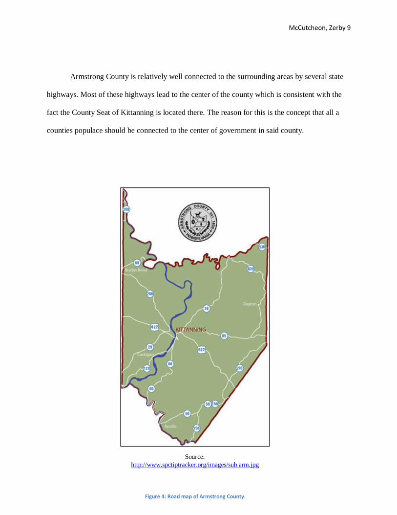
Armstrong County is relatively well connected to the surrounding areas by several state

highways. Most of these highways lead to the center of the county which is consistent with the

fact the County Seat of Kittanning is located there. The reason for this is the concept that all a

counties populace should be connected to the center of government in said county.

Source: http://www.spctiptracker.org/images/sub arm.jpg

Figure 4: Road map of Armstrong County.

http://www.spctiptracker.org/images/sub%20arm.jpg

McCutcheon, Zerby 10

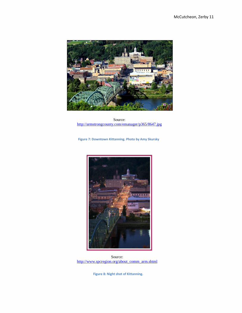
1.3 Current Conditions:

In many ways Armstrong County is a tale of two cities one peaceful and serene and the

other a buzz with activity. This county is home to both the beautiful and tranquil countryside yet

still never a far reach from small-town life as depicted in the following images.

Source: http://armstrongcounty.com/emanager/p365/665.JPG

Source: http://armstrongcounty.com/emanager/p365/8023.JPG

Figure 5: Farm and its covered bridge in winter photo by Marge van Tassel.

Figure 6: Colorful Leaves. Photo by Gloria A. Fawcett.

http://armstrongcounty.com/emanager/p365/665.JPG

http://armstrongcounty.com/emanager/p365/8023.JPG


Source: http://www.spcregion.org/about_comm_arm.shtml

Source: http://armstrongcounty.com/emanager/p365/8647.jpg

Figure 7: Downtown Kittanning. Photo by Amy Skursky

Figure 8: Night shot of Kittanning.

http://www.spcregion.org/about_comm_arm.shtml

http://armstrongcounty.com/emanager/p365/8647.jpg


History:

This county was named after John Armstrong from Carlisle, Pennsylvania. He was a

member of the Continental Congress and served in the Revolutionary War as a Major General.

Armstrong County was home to three huge industries in the 1800s: oil, iron, and glass.

The oil industry was located at the top of the county in the city of Parker. With more than 20,000

residents in the late 1800s, the industry there stagnated and turned the population of the former

city into a small village of around 800.

Source: http://www.history.army.mil/books/Sw-SA/Armstrong.htm

Figure 9: John Armstrong. Painting by Daniel Huntington after John Vanderlyn. Oil on Canvas, 36" x 29", 1873

http://www.history.army.mil/books/Sw-SA/Armstrong.htm


Two towns in Armstrong County had lucrative industry: iron in Brady’s Bend and plate

glass in Ford City (later known as Pittsburgh Plate and Glass).

Brady’s Bend was once known as the “Pittsburgh of the Middle 1800s” because of the

amount of iron and steel it produced. The Brady’s Bend Iron Company was the first to produce

T-rails west of the Allegheny Mountains.

In the late 1800s, Ford City was a “company town” of Pittsburgh Plate Glass Company

and employed almost 2000 people. Pittsburgh Plate Glass Company (PPG) in Ford City was an

Source: http://www.elibrary.dep.state.pa.us/dsweb/GetRendition/Document-

75594/html

Figure 10: Brady's Bend, Pennsylvania

http://www.elibrary.dep.state.pa.us/dsweb/GetRendition/Document-75594/html

http://www.elibrary.dep.state.pa.us/dsweb/GetRendition/Document-75594/html


enormous factory, spanning twenty acres. The population of the town was close to 5000 in its

heyday. The plant shut down in 1991.

Source: http://www.history-map.com/picture/002/Pennsylvania-City-Ford.htm

Figure 11: Ford City, Pennsylvania. 1896

http://www.history-map.com/picture/002/Pennsylvania-City-Ford.htm


Initiatives:

Armstrong County’s planning division is currently seeking to improve roadways and

bridges within the county. A multi-year study of Kittanning is also currently in process. This

study is being used to link the river to the trails, improve pedestrian traffic, and make better use

of transit stops. The idea behind this study is to create and implement a plan which will allow

better foot, bicycle, vehicle, and transit flow not only in Kittanning but also in towns throughout

the entire county.

The planning division also develops local ordinances and oversees zoning codes for the

county. Housing, municipal waste and recycling programs are other initiatives of the planning

division.

Figure 12: Armstrong County historical timeline 1800-1900


The county created a conservation, greenway, and open space plan in 2009. This plan

provided an analysis of the current park and recreation system, public needs and opinions, and

numerous businesses and local organizations. It provides an all-inclusive plan to make the county

a safe place to work, live, and play which will greatly improve the quality of life of the county’s

citizens and its natural resources.


Chapter 2.0 introduction

This chapter is dealing with demographics. Demographics give great insight into the

question of who makes up the population being examined. This chapter will be broken into five

sections each looking at a particular portion of the demographics for Armstrong County, PA. The

first section will examine the county’s population as a whole looking at key factors such

population size and growth rates. Section 2.2 will take a look at urbanization trends.

The following section will discuss the age and sex distribution of the population. Section

2.4 will examine the race distribution of the population. The final section will look at the makeup

of households for the county. The data used for the following analysis is sourced from both

http://www.census.gov/, and http://www.socialexplorer.com/.

Chapter 2.1 Population Characteristics and Trends

Population Density Map 2000 Source:http://www.socialexplorer.com/

Population Density Map key Source:http://www.socialexplorer.com/

Population Density Map 2010 Source:http://www.socialexplorer.com/

Figure 13: Population density map comparison from 2000 to 2010.

http://www.census.gov/

http://www.socialexplorer.com/








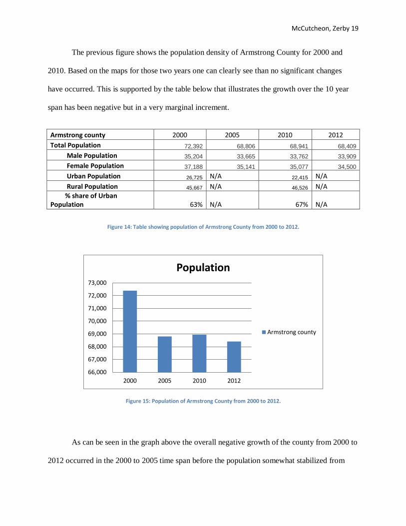
The previous figure shows the population density of Armstrong County for 2000 and

2010. Based on the maps for those two years one can clearly see than no significant changes

have occurred. This is supported by the table below that illustrates the growth over the 10 year

span has been negative but in a very marginal increment.

Armstrong county 2000 2005 2010 2012 Total Population 72,392 68,806 68,941 68,409

Male Population 35,204 33,665 33,762 33,909

Female Population 37,188 35,141 35,077 34,500

Urban Population 26,725 N/A 22,415 N/A Rural Population 45,667 N/A 46,526 N/A % share of Urban Population 63% N/A 67% N/A

Figure 14: Table showing population of Armstrong County from 2000 to 2012.

Figure 15: Population of Armstrong County from 2000 to 2012.

As can be seen in the graph above the overall negative growth of the county from 2000 to

2012 occurred in the 2000 to 2005 time span before the population somewhat stabilized from

66,000

67,000

68,000

69,000

70,000

71,000

72,000

73,000

2000 2005 2010 2012

Population

Armstrong county


2005 to 2012. This drop may warrant further review to determine what factors were in play that

lead to a drop in population nearing 4000 people.

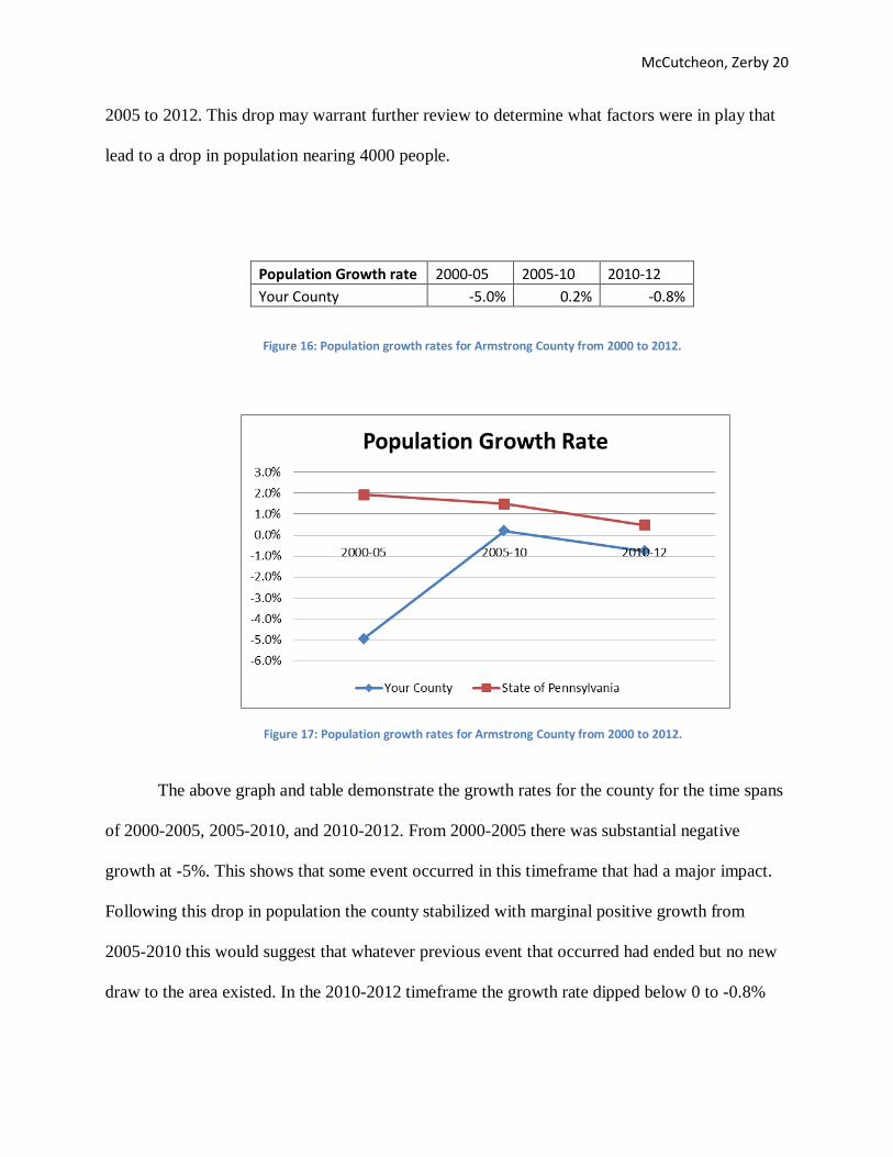
Population Growth rate 2000-05 2005-10 2010-12 Your County -5.0% 0.2% -0.8%

Figure 16: Population growth rates for Armstrong County from 2000 to 2012.

The above graph and table demonstrate the growth rates for the county for the time spans

of 2000-2005, 2005-2010, and 2010-2012. From 2000-2005 there was substantial negative

growth at -5%. This shows that some event occurred in this timeframe that had a major impact.

Following this drop in population the county stabilized with marginal positive growth from

2005-2010 this would suggest that whatever previous event that occurred had ended but no new

draw to the area existed. In the 2010-2012 timeframe the growth rate dipped below 0 to -0.8%

Figure 17: Population growth rates for Armstrong County from 2000 to 2012.


this slight but notable negative growth could indicate a new push factor is now in play, an old

pull factor has died out, or that death rates are outpacing birth rates.

Chapter 2.2 urbanization trends

The urban population in Armstrong County is vastly different than the same population

of the state of Pennsylvania. Armstrong County has no large cities in its area and that is one

reason most of the residents live in rural areas. Another reason is the geography of the county. It

is made up of mainly forest area, hills and valleys, so that is another factor at play as to why the

population is based mainly in rural areas.

The following two charts give a comparison of Armstrong County and the state of

Pennsylvania in 2000 and 2010. The data was sourced from census.gov and it is clearly shown

that Armstrong County is more of a rural population than urban and that most of the state of

Pennsylvania shows an urban population.

Figure 18: Armstrong County Urban and Rural population trends in 2000 and 2010.


The following two graphs show Armstrong County and Pennsylvania’s population

percentages as per housing units. Rural population in the county in 2000 was estimated at 62%,

far above the rural population for the state.

Figure 20: Percentage share of Urban vs Rural population in Armstrong County in 2000

Figure 19: Pennsylvania Urban and Rural population trends in 2000 and 2010.


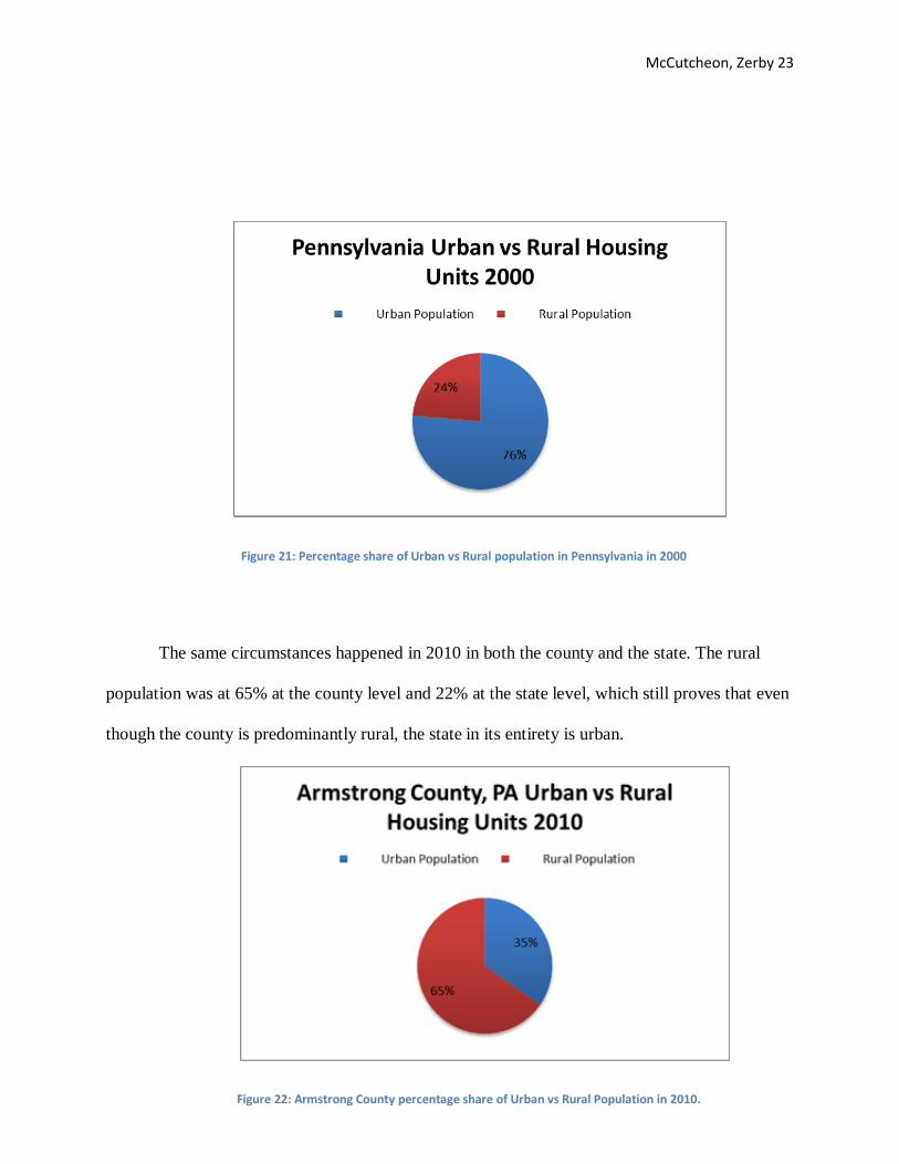
The same circumstances happened in 2010 in both the county and the state. The rural

population was at 65% at the county level and 22% at the state level, which still proves that even

though the county is predominantly rural, the state in its entirety is urban.

Figure 21: Percentage share of Urban vs Rural population in Pennsylvania in 2000

Figure 22: Armstrong County percentage share of Urban vs Rural Population in 2010.


Chapter 2.3 population distribution: age sex

Figure 23: Pennsylvania percentage share of Urban vs Rural population in 2010.

Figure 24: Armstrong County population pyramid in 2000.


The graph above is the population Pyramid for the county of Armstrong in the year 2000.

This graph best demonstrates the composition of age and sex. Though this may seem like a

snapshot of the county’s population composition it is much more than that this graph tells a story

of historical population trends.

For example one may simply see that the 35-44 age range is the largest population group

but what that age range also suggests is that in roughly 1965 the county was in the peak stages of

a baby boom. This graph goes on to show the population of the county is aging and that needs of

the elderly are going to be in high demand. This graph also shows that though the population is

having negative growth the younger population that followed the suggested boom may be

somewhat more stabilized at a lower total population. The sex distribution is just about even and

would be what one would expect to see in a stable region.

Figure 25: Armstrong County population pyramid in 2012.


This graph derived from the age sex distribution in 2012. This graph is consistent with

what one would expect for a stable region as far as sex distribution is concerned. The graph also

supports the conclusions made for the population in 2012 as no major changes occurred and the

bulge caused by the suspected baby boom moved up in age. A second observation is that the

younger population has stabilized over the 12 year difference between graphs.

Chapter 2.4 population distribution: Race

This section will talk about the population distribution of race from the years 2000 until

2012. In 2000, according to census.org, the overall county population was 72,392. Of this

population count, the percentage of white people alone was 98%, which means that the county is

predominantly white. This trend stays the same in 2012 which shows that there isn’t a significant

racial distribution in the area.

While the population of the county has been significantly white throughout the twelve-

year span of this census data, there have been some changes in the other ethnic populations. The

black or African American population showed an increase from 2000 to 2005, then dropped in

2010 then increase again by 2012.

Also, there was a huge increase in the American Indian and Alaskan Native alone

population between the years 2000 and 2005, and then a sharp decline through 2010 and 2012. It

is not known the sudden surge and decline of this particular population but it could have been

due to employment or cultural factors.


The chart above shows the figures that were collected during the census-taking periods of

2000, 2005, 2010, and 2012. This concludes that while the population is predominantly white,

Armstrong County does have a small ethnic base to its population.

The two following charts also show that Armstrong County was a predominantly white

county in both 2000 and 2012. This could be because the main people whom originally settled in

Armstrong County were the Anglo-Europeans.

2000 2005 2010 2012Total Population 72,392 69,664 68,941 68,659

White alone 71,173 68,562 67,565 67,203Black or African American alone 592 694 553 611

American Indian and Alaska Native alone66 408 45 33

Asian alone 89 N 150 128Native Hawaiian and other Pacific Islander alone 13 N 9 0Some Other Race alone 97 N 91 182Two or More Races 362 N 528 502

Figure 26: Armstrong County population by race.

Figure 27: Armstrong County racial population distribution in 2000.


Chapter 2.5 Household characteristics

This section will introduce the average household structure and family size in Armstrong

County, PA during the years of 2000 to 2012. It is suggested from this data that in the years of

2000 and 2010, the most common was a 2-person household.

The total number of households in the county in 2000 was estimated at 29,005 with an

average household size of 2.46 as opposed to the year 2012 where the total households were

estimated at 28,298 with an average household size of 2.36 showing a small drop in the county.

The following chart shows the differences between 1-person households to 4-person

households in both the county and the state from 2000 to 2012. It really doesn’t show a

Figure 28: Armstrong County racial population distribution in 2012.


significant increase or decrease within the numbers of people per household throughout all four

years and in the state.

Figure 29: Armstrong County household population from 2000-2012.

Figure 30: Pennsylvania household population from 2000-2012.


The following four graphs also help the reader grasp the difference of household size in

2000 and 2010 in the state and county. It shows that the family units stay the same over a ten

year period.

Figure 31: Average household size in Armstrong County and Pennsylvania in 2010


Figure 32: Average household size in Armstrong County and Pennsylvania in 2000.


Throughout the course of ten-year span, Armstrong County really hasn’t changed all that

much. The housing data prove the little variation in change but it also shows there isn’t much of

a change within the entire state. This could be because of economic decline or various other

reasons.


3.0: Introduction

This chapter will discuss and analyze Armstrong County’s labor force, employment

trends, industry trends and commuting patterns within the years 2000 to 2012 and compare it

with the state of Pennsylvania as a whole. The chapter will entail four sections each focusing on

individual areas over the previous said period of time. Section 3.1 will discuss the characteristics

of the county’s labor force of the population whom are 16 and older. This section will also

analyze the educational attainment for peoples above the age of 25 and compare it with the state.

Section 3.2 focuses on employment and unemployment rates and the trends within those two

characteristics, again over the same period of time from 2000 to 2012.

Section 3.3 analyzes the earnings by industry in the county over the twelve year span per

capita and compares it to the state earnings by industry. Section 3.4 breaks down the commuting

patterns for the populationof the county. It will provide the average commuting time for the

population to drive to work within the county and compare it to the commuting times in the state.

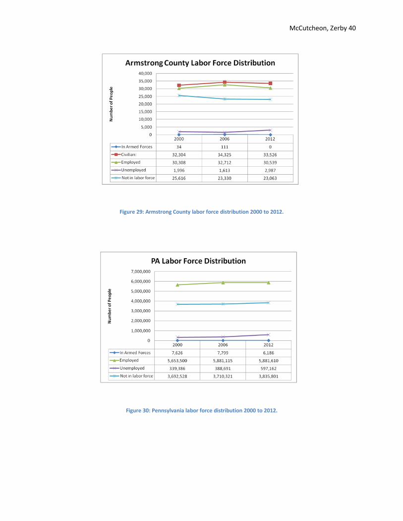
3.1: Labor Force Characteristics

It is important to show labor force trends in order to explain what the economy is like in

the county. Keep in mind from Chapter 2 that the total population for Armstrong County in 2000

was 72,392, only 45% of the population 16 and above at the time was in the labor force.In 2006,

the total population of the county was 68,806; here the population decreased; the percentage of

people in the labor force increased to 46%. That’s less than half the population of the county in

the labor force stimulating the economy.

The population stayed about the same in 2012 and the population in the labor force

increased a little bit to 49%. This can be perceived as the economy getting better by that year.


Figure 33: Armstrong County vs Pennsylvania comparison of in or not in the labor force distribution in 2000.


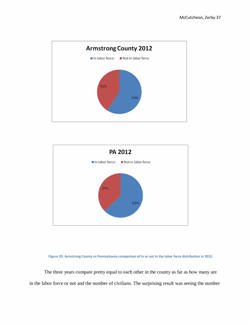
The three years compare pretty equal to each other in the county as far as how many are

in the labor force or not and the number of civilians. The surprising result was seeing the number



of people in the Armed Forces slide from 34 down to zero in 2012; assuming that these were

active military in full-time positions not the weekend guard or reserve units. Also, the number of

unemployed jumped a bit between the years 2006 and 2012. This could be attributed to a weak or

weakening economy.

Compared to Pennsylvania, the total population in 2000 was 12,281,054 with 49% of the

population 16 and over in the labor force. In 2006, out of a population of 11,979,147, 51% of the

population was in the labor force and in 2012, 51% out of the total population of 12,699,589, 16

and above were in the labor force. This is still probably attributed to a weak economy and

definitely the lack of jobs in the state.

So to compare Armstrong County to the state of Pennsylvania, in 2000, the labor force

was at 45% while there was a slight increase in the state at 49%. In 2006, there was still a slight

increase in the state at 51% while the county employed a population of 46%, and in 2012, 51%

of the labor force 16 and over at the state level is still an increase over the 49% in Armstrong

County. This could be attributed to the entire state having concentrated urban centers while

Armstrong County has a higher percentage of rural area.


Figure 36: Labor force percentage for Armstrong County and Pennsylvania from 2000 to 2012.


Figure 29: Armstrong County labor force distribution 2000 to 2012.

Figure 30: Pennsylvania labor force distribution 2000 to 2012.


An important fact when looking at the quality of the labor force in Armstrong County and

comparing them to the state of Pennsylvania is educational attainment. The numbers are higher

of those over 25 years old who have a high school diploma than any other type of degree or non-

degree. The order of educational attainment is: less than high school, high school diploma, some

college, bachelor’s degree, master’s degree, professional school degree, and doctoral degree.

This is at both the county and state level. Reiterating that the population numbers of high school

diploma earners rank at the top while the number of persons with a doctoral degree is the least in

terms of educational attainment.


Figure 39: Educational attainment for Armstrong County and Pennsylvania from 2000 to 2012.


3.2: Employment and Unemployment Rate

This section will analyze the differences in employment and the unemployment rate

throughout the county and compare it to the state.

In Armstrong County in the year 2000, of the population 16 and over, 6% was

unemployed compared to 94% employed. In 2006, that comparison was also a 5%

unemployment rate compared to 95% of the 16 and over population being employed. In 2012 the

unemployment rate was 9% with the employment rate being 91%. The three years compare

pretty evenly with the slight increase of unemployment in 2012.

Figure 40: Armstrong County vs Pennsylvania employment in 2000.



The state employment and unemployment rates are as follows: in 2000, the

unemployment rate was 6% compared to the employment rate at 94%; in 2006 the

unemployment rate was 6% compared to the employment rate at 94%; and in 2012 the

unemployment rate was 9% compared to the employment rate at 91%. The rates of the state

seem to stay pretty steady as far as both employment and unemployment are concerned with a

slight increase in unemployment and decrease in employment in 2012.

These numbers all compare the unemployment and employment to the age years of 16

and up and not the total population in both Armstrong County and Pennsylvania. This is the age

a person can legally start working.

Comparing the state and the county, it is seen that there is only a 1% increase of

unemployment in the state as opposed to the county and slightly more of an increase per each of

the three years in the employment rates in the state in comparison to the county. This is

regardless of whether there was a population decline or increase in any of the three years.



3.3: Earnings by Industry

In this section we will examine the Earnings by industry for Armstrong County. Below

are graphics that outline the percent makeup and growth trends for Armstrong County and the

state of PA for comparison.

Figure 43: Earnings by industry in Armstrong County and Pennsylvania in 2000.


The graphs above show the comparison of Armstrong to Pa percent earnings by industry. This

information is helpful in determining what sectors of the county produce the most earnings as well as

determining where the county stands compared to the rest of the state. As you can see from the graph



agriculture plays a large and growing role in the economy of Armstrong however this is in stark

comparison to the state where agriculture accounts for only 1%. This could indicate that most of the state

is moving into other sectors while Armstrong County absorbs the demand from the rest of the state. One

area of caution for the county may be that of the Professional Sector slight decreases in this sector for the

county while the rest of the state seems to be growing in this sector may be cause for alarm. This issue

could either indicate that there is a brain drain occurring, or that the county is missing out on an

expanding sector.

The following graphs show the comparative economic growth of Armstrong County compared to

that of PA. These graphs show that the earnings by industry are for the most part stable with noticeable

growth in a few sectors, and minimal decreases from 2006 to 2012 that more or less show a return to 2000

levels. This is in stark comparison to the state where earnings by industry seem to be on a steady rise for

all sectors but manufacturing.


Figure 46: Armstrong County to Pennsylvania comparison of earnings by industry growth.


3.4: Commuting Pattern

This section will look at the commuting patterns of Armstrong County, PA. For this

purpose the average commute time for the county will be compared to that of the state of PA.

The average commute time for the state will act as a baseline to determine if any significant

deviation from the state trend exists. To start this section let us first examine the graph below.

As one can see the average commute time for the state and the county in 2000 have a

difference of 2 minutes. This fact shows that on average that the people in Armstrong live two

minutes further from work than the state average. Next, one sees that the average time commute

for Armstrong county drops to a level that is on par with the state. This could suggests that either

people in the county have moved closer to work, gotten job closer to home or traffic conditions

Figure 49: Graph of average commute times from 2000 to 2012.


effecting commute times have improved. The final shift is substantial. In 2012 one can see that

the people of Armstrong County have added Five minutes to their commutes on average. Even

though the average for the state has increased Armstrong County has outpaced the trend of the

state. This could suggest that people have moved further to work, gotten job further from home

or traffic conditions effecting commute times have worsened. On a whole Armstrong County is

not massively off the State average but a community should strive to keep commute times low to

decrease economic losses and improve quality of life.

The Average commute times for a community have a major impact on the economy as

well as quality of life. The economic impacts of extending commute times include lose of

productivity, expenses of gas, and the cost of vehicle maintenance. Commute times impact

quality of life by taking time away from possible family or recreational activities.


4.0 Introduction:

The purpose of this chapter is to discuss the results of an economic analysis done on

Armstrong County and supply the methodology used to provide these results. The economic data

used was gained from the Bureau of Economic Analysis (www.bea.gov).

This analysis was conducted by determining the basic employment and comparing it to

the non-basic employment of the county using employment population figures. Three years were

used in this analysis: 2001, 2006, and 2012. Population figures per industry were used as the

guideline. The analysis uses the location quotient tool with each year in this study to compare

the local economy to the larger Pennsylvania economy. A ratio is provided upon using this tool

for the county to compare to the state.

4.1: Economic Base Analysis:

The reason planners perform an economic base analysis for their particular area is to find

out what industries are doing well and what industries are the weakest. This helps determine

what types of industries to bring into the area in order to help the local economy. These base

industries are the main supporters and provide the largest revenue to the economy.

The following chart shows the total industry population figures for 2001 in Armstrong

County. This chart shows that the three largest economic contributors in Armstrong County at

the time were: manufacturing; education, health and social services; and retail trade. It also


shows the three weakest areas: wholesale trade; information; and public administration. This

suggests that the county is more of a rural area and has lower population income than other areas.

It could also mean that the area has a middle-aged to older population. Basic employment, which

was discussed in the previous paragraph, in 2001 was 4,262 and the secondary sector industries

employment was 30,308. This means that more of the population works in the service industry

than in the main productive economic industries.

Figure 50: Armstrong County Industry Totals 2001.

The next chart shows that in 2006 the same three industries are the top three:

manufacturing; education, health and social services; and retail trade. It also shows that there

hasn’t been much of a difference in industries as a whole. This is suggestive that nothing has

moved into or out of the county. Industries that are the weakest are: information, wholesale trade,

Industries/ Economic Sectors by NAICS Code Armstrong Agriculture, forestry, fishing and hunting, and mining 1,279 Construction 2,146 Manufacturing 6,586 Wholesale trade 903 Retail trade 3,792 Transportation and warehousing, and utilities 2,072 Information 533 Finance, insurance, real estate, and rental and leasing 1,006 Professional, scientific, management, administrative, and waste management services

1,473

Educational, health and social services 5,914 Arts, entertainment, recreation, accommodation and food services

1,967

Other services (except public administration) 1,726 Public administration 911

Total Employment 30,308


and public administration. In 2006, the base employment was 3,703 with most of the population

working again in the service industry to supplement the base industries at25,962.

Figure 51: Armstrong County Industry Totals 2006.

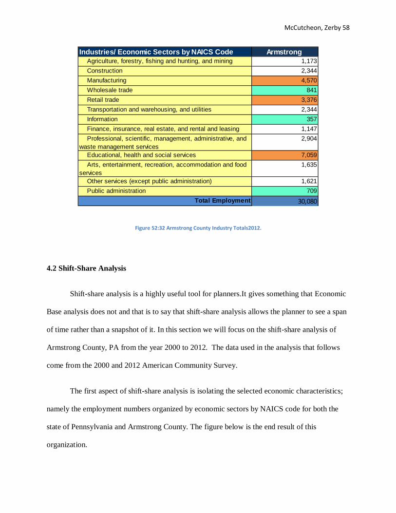
In 2012, the top three industries were still manufacturing, retail, and educational, health

and social services with the weakest still being information, wholesale trade, and public

administration, as shown by the following chart. The base employment population was 5,138 and

the non-basic employment figure was 24,942. This again shows that there hasn’t been much

change in the eleven-year span in employment industries. It shows that most of the population

still worked in the service industry.


1,746


2,300


Total Employment 29665


Figure 52:32 Armstrong County Industry Totals2012.

4.2 Shift-Share Analysis

Shift-share analysis is a highly useful tool for planners.It gives something that Economic

Base analysis does not and that is to say that shift-share analysis allows the planner to see a span

of time rather than a snapshot of it. In this section we will focus on the shift-share analysis of

Armstrong County, PA from the year 2000 to 2012. The data used in the analysis that follows

come from the 2000 and 2012 American Community Survey.

The first aspect of shift-share analysis is isolating the selected economic characteristics;

namely the employment numbers organized by economic sectors by NAICS code for both the

state of Pennsylvania and Armstrong County. The figure below is the end result of this

organization.


2,904


1,635


Total Employment 30,080


Figure 53: Employment Numbers Organized by Economic Sectors (NAICS Code).

After organizing the data, the next step is to calculate the change in employment from

2000 to 2012 by subtracting the employment numbers of 2000 from those of 2012. The change

in employment is used in the next step of calculating the percent growth rate. This is done by

dividing the change in employment by the employment numbers of 2000 as seen in the following

figure:

Figure 54: Calculated Change and Growth Rate.

In the figure above one should take notice of the total employment, change, and growth

rates row. This row contains both the growth rates for both the state and county. The growth rate

for Armstrong is -.75% and the state is 4.03%. The state growth rate is a key aspect for shift-


share analysis as not only is it the state growth rate but it is also the state growth effect. The state

growth effect is the amount of growth in a county that is attributed to the growth of the state’s

economy.

Figure 55: Calculated Effects and Total Shift.

The figure above is the final step in shift-share analysis. To calculate the industry mix

effect, the process is to subtract the state growth effect from the state growth rate of an industry.

This number gives an idea of what an industry’s growth would be without the effect from overall

state economic growth. The numbers for industry mix effect for Armstrong can be seen in the

figure above. The next step is to calculate the local share effect. This is what the growth of

industries in the county would be without the aid of state growth. This is calculated by

subtracting the state growth rate of an industry from that of the corresponding county industry.

The numbers for Armstrong can be seen in the figure above. The last step is to calculate the total

shift. This is done by simply adding the state growth effect, industry mix effect, and the local

share effect.

Overall Armstrong has not fared well in the past 12 years with a -228 in total shift. A

large portion of this poor showing can be attributed to heavy losses in the manufacturing sector


compounded with losses in information and retail trade. That being said not all is bad as

staggering growth has occurred in the professional industry as well as education.

4.3 Cluster Analysis

The cluster analysis shown in the chart and graph below is for that of the economics of

Armstrong County. This method of analysis looks at three variables that are calculated for each

of the representative industries. The variables are as follows: the earnings growth rates from

2001 to 2012, the employment growth rates for 2000 to 2012 and the location quotients for 2012.

Description Earnings growth rate Employment growth rate Location

Quotient 2012 2001-12 2000-12

Agriculture, forestry, fishing and hunting, and mining 258% 2% 2.682 Construction 20% 2% 1.391 Manufacturing 27% -29% 1.237 Wholesale trade 197% -13% 1.008 Retail trade 0% -4% 0.947 Transportation and warehousing, and utilities 26% 12% 1.546 Information 20% -29% 0.698 Finance, insurance, real estate, and rental and leasing 23% 0% 0.604 Professional, scientific, management, administrative, and waste management services -3% 47% 0.992 Educational, health and social services 75% 30% 0.897 Arts, entertainment, recreation, accommodation and food services 49% -9% 0.654 Other services (except public administration) 29% -6% 1.157 Public administration 34% 4% 0.572

Figure 56: table of earnings growth employment growth and LQ.


For a better understanding of the information presented in the table above the variables

were can be place in a bubble graph that utilizes x, y, and z axis. The x axis represents the

earnings growth rate. The y axis represents the employment growth rate. The z axis which is seen

by the size of the representative bubbles shows the size of the LQ. As can be seen in the graph

below the majority of the industries are clustered near the 25, -10 mark but there are a few

outliers that demand attention. The industries of agriculture and wholesale trade are far outpacing

the other industries in earnings growth while having minimal to negative growth in employment.

The other outlier is that of the professional industry. This industry sits at -3, 47 which means that

earnings have decreased as employment has spiked.


Figure 57: Bubble chart of Cluster Analysis for Armstrong County.

-60%

-40%

-20%

0%

20%

40%

60%

80%

-50% 0% 50% 100% 150% 200% 250% 300% 350%

Empl

oym

ent g

row

th

Earnings Growth

Cluster Analysis for Armstrong County 2000-2012

Agriculture, forestry, fishing and hunting, and mining

Construction

Manufacturing

Wholesale trade

Retail trade

Transportation and warehousing, and utilities

Information

Finance, insurance, real estate, and rental and leasing

Professional, scientific, management, administrative, andwaste management services Educational, health and social services

Arts, entertainment, recreation, accommodation and foodservices Other services (except public administration)

Public administration


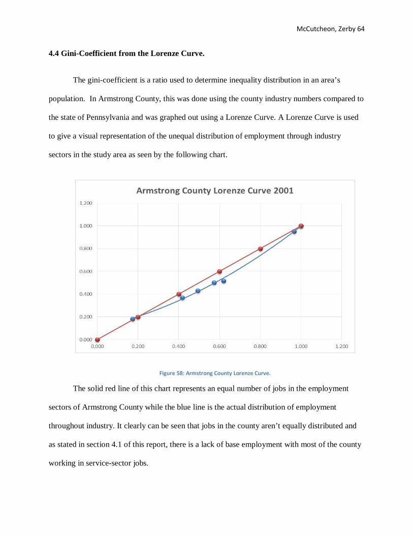
4.4 Gini-Coefficient from the Lorenze Curve.

The gini-coefficient is a ratio used to determine inequality distribution in an area’s

population. In Armstrong County, this was done using the county industry numbers compared to

the state of Pennsylvania and was graphed out using a Lorenze Curve. A Lorenze Curve is used

to give a visual representation of the unequal distribution of employment through industry

sectors in the study area as seen by the following chart.

The solid red line of this chart represents an equal number of jobs in the employment

sectors of Armstrong County while the blue line is the actual distribution of employment

throughout industry. It clearly can be seen that jobs in the county aren’t equally distributed and

as stated in section 4.1 of this report, there is a lack of base employment with most of the county

working in service-sector jobs.

Figure 58: Armstrong County Lorenze Curve.


5.0 Introduction

This chapter focuses on what Armstrong County can do for the future based on the

demographic and economic analysis that was discussed in the previous chapters. The first section

will both explain and identify what is known in strategic planning as a SWOT analysis. The

second section of this chapter will provide four key areas and will identifyfuture development

strategies. The chapter will conclude with strategy proposals for Armstrong County.

5.1 SWOT Analysis

SWOT stands for strengths, weaknesses, opportunities and threats. It is primarily used by

organizations, businesses, and local governments to gain insight into what the organization’s

internal strengths and weaknesses are and what kind of external opportunities and threats may

exist.

Figure 59: SWOT Analysis diagram


To perform a SWOT analysis, the organization must first determine what the main

objective or objectives are. Once those objectives are known, the SWOT analysis can help

determine what to change or not change to achieve the stated objectives. The SWOT section will

be broken down into each specific category of the analysis.

Strengths

Armstrong County has many identifiable strengths; some of which will be discussed here.

The county has an abundance natural and physical features in terms of rivers, lakes, and streams

to attract visitors to the area. The rivers and lakes can and are used for fishing, boating, and

water-skiing. Streams are mostly used for fishing or catching bait to fish with. The abundance of

park land in Armstrong County also can draw visitors to the area. The location of the county and

a main artery straight from the city of Pittsburgh can prove beneficial to bringing tourism and

recreation to the county.

The population of the county is mostly middle-age which is beneficial because it means

that people of that age bracket tend to own property and have better paying jobs to keep the

economy at a level. The household size also brings stability to the county by means of the

economy.

Even though the days are gone of the oil, iron, and glass industries in the county,

agriculture has taken the forefront of being the economic strength of the area. There are many

farms and farmers in the county to help generate local income with their harvests and

accessibility to fresh meat for the citizens.

Weaknesses


The main artery to the city of Pittsburgh is not only a strength but a weakness for the

county. The reason for this is that it gives the county population direct access to the city of

Pittsburgh, taking monies out of the county and contributing to other economies.

As the majority of the county is rural, this poses to weaken the economy as the

population has to utilize automobile transportation thus taking their business and employment

elsewhere. It also lacks the sales income from major shopping centers that adjoining counties

have. Another weakness is that the county has a large number of elderly citizens. This population

doesn’t generate a large amount of income for the economy because they are retired or unable to

gain employment due to their age and individual circumstances.

The lack of industry also weakens the county economy because it doesn’t generate jobs

and money to give back to the area. Unemployment issues could be correlated to the lack of

industry in the county, as the unemployment rate is at 9%. The population that travels out of the

county for employment spends on gasoline and other secondary industries usually where they are

employed because of the lack of business in the county.

Higher education is also lacking in the county. Many of the younger generation who go

on to higher education generally move out of the area and don’t partake in what goes on in the

local economy. The same goes for population earnings. Those that have the education, move

where they can make more money.

Opportunities

Armstrong County has such vast natural resources in its lakes, rivers, rolling hills, and

game lands, a huge opportunity for the county is to take the natural areas and promote tourism. It

is also an area rich in history. The location to Pittsburgh could attract city dwellers into the

county if more was done to push the county as the great outdoors.


Another opportunity the county could capitalize on is giving the younger, college-

educated generation a reason to stay. Bring technological industries into the county to coincide

with the tourism industry and thus boost the economy of the county.

Threats

Flooding is always a concern to the county because of the many water resources located

in the area. Flooding reduces the amount of land being sought after and purchased to bring

industry in. Flash flooding puts the population and recreation population in danger and this

doesn’t look good for the county.

The predominant race of the county is white and this poses a threat because there isn’t a

diverse culture to appeal to a broader audience. When there isn’t broad appeal in an area, there

won’t be a large amount of outsiders who come to spend their money in the county.

The lack of industry and the unemployment rate is a definite threat to the economy of the

county and can only be rectified by bringing more industry into the area.


5.2 Future Development Strategies

With the booming gas industry in our region it would be foolhardy not to take full

advantage in the potential economic influx to the county. Several key strategies should be

implemented to increases the viability of this industry while maintaining the charm and distinct

characteristics of the community and preparing for possible gains in other economic areas.

Locality Development Strategies:

Infrastructure Provisions:

First and foremost we should make every effort to build up the demanded infrastructure

required for a thriving gas industry. This is a mammoth undertaking as many facets of this

industry are interdependent. One key area that should be overhauled is that of transportation.

Transportation is critical to the rapid and efficient deployment of goods, materials, personal, and

services that all industry sectors require. The building of new and improving of existing

roadways, and railways would greatly impact the viability of the gas industry and other

industries directly but this would also aid in the development of other areas of infrastructure.

Next the development of gas pipelines should be approach in a systematic manner that would

allow for rapid deployment of new gas wells as well as efficient transport of gas to refining

stations. The development of a high speed telecommunication system should be employed to

meet if not excide the demands of the technical fields. The aforementioned improvements would

most certainly allow the gas industry as well as other industries to take note of the potential for

development in the county.


Zoning Regulations:

Armstrong County has a unique characteristic created by a blending historical importance

with modern relevance, and rural charm with urban excitement. Careful consideration should be

given to the development of zoning strategies that protect the identity of the county while not

hindering the development of industry. Not many people would claim that the visibility of

pipelines and gas wells add value to the scenic vistas provided by nature. Zoning regulations

could offer a way to mitigate issues such as these by implementing rules as to where and how

such structures are built. Furthermore certain style of new construction buildings would detract

from the charm of historical districts and towns. Consideration should be given to regulations

that encourage methods that protect certain areas while allowing for a more appropriate blending

of old and new in other areas. Finally, methods should be employed that insulate residential areas

from the potential incursion of business development. This insulation would service to protect

both quality of life as well as property values.

Business Development Strategies:

Technology and Business Parks:

Any single business does not exist in a vacuum that is to say that a business is

reliant upon the resources, and services provided by other business entities as much as they are

reliant on the demand for their product by consumers. Technology and Business Parks offer

incentive to potential investment of businesses into the county by creating a central location

where the commerce of that particular industry is focused. In the case of the promotion of the gas


industry in the county a Technology and Business Parks could be setup in a manner that allows

for rapid communication between gas extraction companies, refinement companies, and

engineering firms. This would also have the added effect of making a visual statement as to why

individuals with the backgrounds and educations necessary for the conducting of such business

should stay within the county or as to why they should relocate to the county.

Enterprise zones:

Armstrong County should strive to bring in new forms of industry and bolster emerging

industries. One strategy to achieve this would be to offer enterprise zones. These are zones that

establish incentives for companies to invest the capital required to establish a foothold in the

county. One possible area where an enterprise zone may be seen as a smart choice would be to

offer tax incentives or relief if a company were to build a gas refinement plant. Such plants are

costly to construct. The building of such a plant would indicate a commitment to the area as well

as an influx of employment opportunities.

Human resource development strategies:

Customized training:

Armstrong County is most certainly lacking in one critical area and that is higher

education. Consideration should be given to developing a county community college as well as

attracting universities to open a campus within the county. This is of high importance as there are

currently no options for individuals that allow for continuing education within the county. This

impacts the quality of life in the county as well as being a standing push factor for the youth of

the county that wish to attend an institute of higher education.


Training Programs:

Job training programs such as vocational schools could do much in the way of improving

the level of qualification of the population. This combined with the increased job opportunities

offered by the gas industry would do much to decrease the unemployment rate. Training

programs could even bolster the agriculture industry that is currently the linchpin to the economy

of the county. Training programs could offer farmers a not only a lesson in best practices but also

methods to produce more efficiently.

5.3 Conclusion:

The preceding text has been a compilation of information that shows were the county has

come from, where it currently stands, and most importantly what it could be with careful

guidance. The Armstrong has seen its share of missteps but it still stands strong and proud. in

chapter one we gave a brief introduction to the county. In chapter two we introduced you to the

people of the county by way of demographics. Chapter three was all about the economic.

Chapter four was a look at the workforce trends of Armstrong. Finally, in chapter five we

discussed SWOT analysis and future development strategies.


Figure 1: Map of the counties of Western Pennsylvania with Armstrong County highlighted Pg 7. Figure 2: Map showing the 10 counties of the Pittsburgh metropolitan area Pg 7. Figure 3: Map of the townships, boroughs and cities of Armstrong County Pg 8. Figure 4: Road Map of Armstrong County Pg 9. Figure 5: Farm and its covered bridge in winter photo by Marge Van Tassel Pg10. Figure 6: Colorful Leaves photo by Gloria A Fawcett Pg 10. Figure 7: Kittanning Downtown photo by Amy Skursky Pg 11. Figure 8: Downtown Kittanning. Photo by Amy Skursky Pg 11. Figure 9: John Armstrong by Daniel Huntington Pg 12. Figure 10: Brady’s Bend, PA photo Pg 13. Figure11: Ford City, PA 1896 Pg 14. Figure 12:


Armstrong County historical timeline 1800-1900 Pg 15. Figure 13: Population density map comparison from 2000 to 2010. Pg 18. Figure 14: Table showing population of Armstrong County from 2000 to 2012. Pg 19. Figure 15: Population of Armstrong County from 2000 to 2012. Pg 19. Figure 16: Population growth rates for Armstrong County from 2000 to 2012. Pg 20. Figure 17: Population growth rates for Armstrong County from 2000 to 2012. Pg 20. Figure 18: Armstrong County Urban and Rural population trends in 2000 and 2010. Pg 21. Figure 19: Pennsylvania Urban and Rural population trends in 2000 and 2010 Pg 22. Figure 20: Percentage share of Urban vs Rural population in Armstrong County in 2000 Pg 22. Figure 21: Percentage share of Urban vs Rural population in Pennsylvania in 2000 Pg 23. Figure 22: Armstrong County percentage share of Urban vs Rural Population in 2010 Pg 23. Figure 23: Pennsylvania percentage share of Urban vs Rural population in 2010 Pg 24. Figure 24: Armstrong County population pyramid in 2000. Pg 24. Figure 25: Armstrong County population pyramid in 2012. Pg 25. Figure 26: Armstrong County population by race. Pg 27. Figure 27: Armstrong County racial population distribution in 2000. Pg 27. Figure 28: Armstrong County racial population distribution in 2012. Pg 28. Figure 29: Armstrong County household population from 2000-2012. Pg 29. Figure 30: Pennsylvania household population from 2000-2012. Pg 29. Figure 31: Average household size in Armstrong County and Pennsylvania in 2010 Pg 30. Figure 32: Average household size in Armstrong County and Pennsylvania in 2000. Pg 31. Figure 33: Armstrong County vs Pennsylvania comparison of in or not in the labor force distribution in 2000. Pg 35. Figure 34: Armstrong County vs Pennsylvania comparison of in or not in the labor force distribution in 2006. Pg 36. Figure 35: Armstrong County vs Pennsylvania comparison of in or not in the labor force distribution in 2012. Pg 37. Figure 36: Labor force percentage for Armstrong County and Pennsylvania from 2000 to 2012. Pg 39. Figure 37: Armstrong County labor force distribution 2000 to 2012. Pg 40. Figure 38: Pennsylvania labor force distribution 2000 to 2012. Pg 40. Figure 39: Educational attainment for Armstrong County and Pennsylvania from 2000 to 2012. Pg 42.


Figure 40: Armstrong County vs Pennsylvania employment in 2000. Pg 43. Figure 41: Armstrong County vs Pennsylvania employment in 2006. Pg 44. Figure 42: Armstrong County vs Pennsylvania employment in 2012. Pg 44. Figure 43: Earnings by industry in Armstrong County and Pennsylvania in 2000 Pg 45. Figure 44: Earnings by industry in Armstrong County and Pennsylvania in 2006. Pg 46. Figure 45: Earnings by industry in Armstrong County and Pennsylvania in 2012. Pg 47. Figure 46: Armstrong County to Pennsylvania comparison of earnings by industry growth. Pg 49. Figure 47: Armstrong County to Pennsylvania comparison of earnings by industry growth. Pg 50. Figure 48: Armstrong County to Pennsylvania comparison of earnings by industry growth. Pg 51. Figure 49: Graph of average commute times from 2000 to 2012. Pg 52. Figure 50: Armstrong County Industry Totals 2001. Pg 56. Figure 51: Armstrong County Industry Totals 2006. Pg 57. Figure 52: Armstrong County Industry Totals2012. Pg 58. Figure 53: Employment Numbers Organized by Economic Sectors (NAICS Code). Pg 59. Figure 54: Calculated Change and Growth Rate. Pg 59. Figure 55: Calculated Effects and Total Shift. Pg 60. Figure 56: table of earnings growth employment growth and LQ. Pg 61. Figure 57: Bubble chart of Cluster Analysis for Armstrong County. Pg 63. Figure 58: 58: Armstrong County Lorenze Curve. Pg 64. Figure 59: SWOT Analysis diagram Pg 66.


Bibliography Mcclean, Mary L., and Kenneth P. Voytek, 1992. Understanding Your Economy: Using Analysis to Guide Local Strategic Planning. Chicago: Planners Press (American Planning Association). Green Leigh, Nancey, and Edward J. Blakely. 2013. Planning Local Economic Development: Theory and Practice (5th Edition). California: Sage Publications. www.Census.gov www.socialexplorer.com www.co.armstrong.pa.us/ www.armstrongcounty.com

http://www.census.gov/


http://www.co.armstrong.pa.us/

http://www.armstrongcounty.com/

armstrong county planning project report€¦ · armstrong county planning project report . shawna...

Documents