aspects of design and analysis of cognitive radios and
TRANSCRIPT

Aspects of Design and Analysis of
Cognitive Radios and Networks
Muhammad Fainan Hanif
A thesis submitted in fulfillment
of the requirements for the degree of
Doctor of Philosophy
in
Electrical and Electronic Engineering
University of Canterbury
Christchurch, New Zealand
September 2010

i

ii

Abstract
Recent survey campaigns have shown a tremendous under utilization of the band-
width allocated to various wireless services. Motivated by this and the ever increas-
ing demand for wireless applications, the concept of cognitive radio (CR) systems
has rendered hope to end the so called spectrum scarcity. This thesis presents var-
ious different facets related to the design and analysis of CR systems in a unified
way. We begin the thesis by presenting an information theoretic study of cognitive
systems working in the so called low interference regime of the overlay mode. We
show that as long as the coverage area of a CR is less than that of a primary user
(PU) device, the probability of the cognitive terminal inflicting small interference at
the PU is overwhelmingly high. We have also analyzed the effect of a key parameter
governing the amount of power allocated to relaying the PU message in the overlay
mode of operation in realistic environments by presenting a simple and accurate
approximation. Then, we explore the possibilities of statistical modeling of the cu-
mulative interference due to multiple interfering CRs. We show that although it is
possible to obtain a closed form expression for such an interference due a single CR,
the problem is particularly difficult when it comes to the total CR interference in
lognormally faded environments. In particular, we have demonstrated that fitting a
two or three parameter lognormal is not a feasible option for all scenarios. We also
explore the second-order characteristics of the cumulative interference by evaluating
its level crossing rate (LCR) and average exceedance duration (AED) in Rayleigh
and Rician channel conditions. We show that the LCRs in both these cases can
be evaluated by modeling the interference process with gamma and noncentral χ2
processes, respectively. By exploiting radio environment map (REM) information,
iii

we have presented two CR scheduling schemes and compared their performance
with the naive primary exclusion zone (PEZ) technique. The results demonstrate
the significance of using an intelligent allocation method to reap the benefits of the
tremendous information available to exploit in the REM based methods. At this
juncture, we divert our attention to multiple-input multiple-output (MIMO) CR
systems operating in the underlay mode. Using an antenna selection philosophy, we
solve a convex optimization problem accomplishing the task and show via analysis
and simulations that antenna selection can be a viable option for CRs operating
in relatively sparse PU environments. Finally, we study the impact of imperfect
channel state information (CSI) on the downlink of an underlay multiple antenna
CR network designed to achieve signal-to-interference-plus-noise ratio (SINR) fair-
ness among the CR terminals. By employing a newly developed convex iteration
technique, we solve the relevant optimization problem exactly without performing
any relaxation on the variables involved.
iv

Acknowledgements
Well, let me begin with the bottom line. In plain words, this thesis would not
have been possible without the superb supervision, brilliant patience and intelligent
tolerance of Prof. Peter J. Smith, my principal supervisor. In addition to learning
‘tricks of the trade’, I have tremendously benefitted from him in terms of acquiring
essential skills for my professional life. No doubt, the years I spent as a PhD student
will go a long way in my life and the memories of this tenure, both pleasant and
bitter ones, will remain ever green in my mind.
I will also like to take this opportunity to extend my thanks to my co-supervisors,
Prof. Desmond P. Taylor and Dr. Philippa A. Martin. Lively discussions with both
of them have been a great source of enthusiasm and learning. Especially, Friday
afternoon tea/coffee meetings with Prof. Taylor have both been fun and a source of
scholarship.
My gratitude also goes to the generous financial support provided by Telecom
New Zealand and National ICT Innovation Institute (NZi3) for my graduate studies.
I am thankful to them for putting their faith in my capabilities and I hope I have
delivered.
I should also express my gratitude to all those who have remained with me in
E338b during these years. Certainly, Abdulla, Tim, Vijay and Krishna top this
list of people. The technical and computer staff, the cleaning staff and all those
who have helped make my stay a pleasant experience deserve both appreciation and
thanks on my part.
Last but by no means least, I would like to dedicate this thesis to the astronomical
patience and forbearance of my family towards me during all these years.
v

vi

Contents
Abstract iii
Acknowledgements v
1 Introduction 1
1.1 Overview of Cognitive Radio Systems . . . . . . . . . . . . . . . . . . 1
1.2 Thesis Contributions . . . . . . . . . . . . . . . . . . . . . . . . . . . 4
1.3 Thesis Outline . . . . . . . . . . . . . . . . . . . . . . . . . . . . . . . 7
1.4 List of Publications . . . . . . . . . . . . . . . . . . . . . . . . . . . . 8
2 Fundamentals of Wireless Communications and Convex Optimiza-
tion Theory 11
2.1 Fading in Wireless Channels . . . . . . . . . . . . . . . . . . . . . . . 11
2.1.1 Correlation Properties of the Received Signal . . . . . . . . . 14
2.1.2 Statistical Models For Fading Channel/Received Envelope . . 16
2.1.3 Path Loss and Shadow Fading . . . . . . . . . . . . . . . . . . 17
2.2 MIMO Communications . . . . . . . . . . . . . . . . . . . . . . . . . 20
2.2.1 MIMO Capacity with Deterministic and Perfect Channel State
Information . . . . . . . . . . . . . . . . . . . . . . . . . . . . 21
2.2.2 MIMO Capacity Under Fading Channel Conditions . . . . . . 23
2.3 Performance Metrics . . . . . . . . . . . . . . . . . . . . . . . . . . . 28
2.3.1 Ergodic Capacity . . . . . . . . . . . . . . . . . . . . . . . . . 28
2.3.2 Outage Capacity . . . . . . . . . . . . . . . . . . . . . . . . . 28
vii

2.3.3 Level Crossing Rate . . . . . . . . . . . . . . . . . . . . . . . . 30
2.4 An Overview of Convex Optimization . . . . . . . . . . . . . . . . . . 31
2.5 Broad Classification of Convex Optimization Problems . . . . . . . . 34
2.5.1 Linear Programs . . . . . . . . . . . . . . . . . . . . . . . . . 35
2.5.2 Conic Programming . . . . . . . . . . . . . . . . . . . . . . . 35
2.5.3 Geometric Programs . . . . . . . . . . . . . . . . . . . . . . . 37
3 Fundamental Capacity Limits of Cognitive Radio Systems 39
3.1 System Model . . . . . . . . . . . . . . . . . . . . . . . . . . . . . . . 42
3.2 The Low Interference Regime . . . . . . . . . . . . . . . . . . . . . . 45
3.2.1 Rayleigh/Rayleigh Scenario . . . . . . . . . . . . . . . . . . . 46
3.2.2 Rayleigh/Rician Scenario . . . . . . . . . . . . . . . . . . . . . 49
3.2.3 Rician/Rayleigh Scenario . . . . . . . . . . . . . . . . . . . . . 50
3.2.4 Rician/Rician Scenario . . . . . . . . . . . . . . . . . . . . . . 50
3.3 An Approximation For The Power Loss Parameter . . . . . . . . . . . 51
3.4 Results . . . . . . . . . . . . . . . . . . . . . . . . . . . . . . . . . . . 54
3.4.1 Low interference regime . . . . . . . . . . . . . . . . . . . . . 54
3.4.2 Statistics of the power loss parameter, α . . . . . . . . . . . . 56
3.4.3 CR rates . . . . . . . . . . . . . . . . . . . . . . . . . . . . . . 58
3.5 Summary . . . . . . . . . . . . . . . . . . . . . . . . . . . . . . . . . 60
4 Interference and Level Crossing Statistics 63
4.1 System Model . . . . . . . . . . . . . . . . . . . . . . . . . . . . . . . 64
4.2 Statistical Characterization of Interference at the Primary Receiver . 66
4.2.1 Interference Due to a Single Cognitive User . . . . . . . . . . 66
4.2.2 Interference Due to Multiple Cognitive Radios . . . . . . . . . 67
4.3 Level Crossing Analysis . . . . . . . . . . . . . . . . . . . . . . . . . . 73
4.4 Instantaneous CR performance . . . . . . . . . . . . . . . . . . . . . 74
4.4.1 LCRs for Rayleigh Fading . . . . . . . . . . . . . . . . . . . . 74
4.4.2 LCRs for Rician Fading . . . . . . . . . . . . . . . . . . . . . 76
4.4.3 Average Exceedance Duration . . . . . . . . . . . . . . . . . . 78
viii

4.5 Results . . . . . . . . . . . . . . . . . . . . . . . . . . . . . . . . . . . 78
4.6 Summary . . . . . . . . . . . . . . . . . . . . . . . . . . . . . . . . . 83
5 Cognitive Radio Allocation Schemes 85
5.1 PEZ Approach . . . . . . . . . . . . . . . . . . . . . . . . . . . . . . 87
5.2 REM Approach . . . . . . . . . . . . . . . . . . . . . . . . . . . . . . 87
5.3 Simulation Results . . . . . . . . . . . . . . . . . . . . . . . . . . . . 91
5.3.1 Exclusion Zone Results . . . . . . . . . . . . . . . . . . . . . . 92
5.3.2 Comparison of Numbers of CRs . . . . . . . . . . . . . . . . . 93
5.3.3 Imperfections in the REM . . . . . . . . . . . . . . . . . . . . 96
5.4 Summary . . . . . . . . . . . . . . . . . . . . . . . . . . . . . . . . . 100
6 MIMO Cognitive Radios with Antenna Selection 103
6.1 System Model . . . . . . . . . . . . . . . . . . . . . . . . . . . . . . . 105
6.2 Analytical Framework . . . . . . . . . . . . . . . . . . . . . . . . . . 107
6.2.1 Exhaustive Search . . . . . . . . . . . . . . . . . . . . . . . . 110
6.2.2 Convex Approximation . . . . . . . . . . . . . . . . . . . . . . 110
6.2.3 Heuristic . . . . . . . . . . . . . . . . . . . . . . . . . . . . . . 112
6.2.4 A Note on Complexity . . . . . . . . . . . . . . . . . . . . . . 114
6.3 Performance Analysis . . . . . . . . . . . . . . . . . . . . . . . . . . . 115
6.3.1 CDF of CR-CR Link with Single Antenna Selection in the
Presence of Multiple Single Antenna PUs . . . . . . . . . . . . 115
6.3.2 Ergodic Capacities . . . . . . . . . . . . . . . . . . . . . . . . 118
6.3.3 Extension to More Realistic Scenarios . . . . . . . . . . . . . . 120
6.4 Results . . . . . . . . . . . . . . . . . . . . . . . . . . . . . . . . . . . 121
6.4.1 MIMO Selection . . . . . . . . . . . . . . . . . . . . . . . . . 121
6.4.2 SISO Selection . . . . . . . . . . . . . . . . . . . . . . . . . . 126
6.5 Summary . . . . . . . . . . . . . . . . . . . . . . . . . . . . . . . . . 130
7 Optimal SINR Balancing in the Downlink of Cognitive Radio Net-
works with Imperfect Channel State Information 131
ix

7.1 System Model . . . . . . . . . . . . . . . . . . . . . . . . . . . . . . . 132
7.2 Analytical Framework . . . . . . . . . . . . . . . . . . . . . . . . . . 134
7.2.1 Problem Formulation . . . . . . . . . . . . . . . . . . . . . . . 135
7.2.2 Approximate Solution of P1 . . . . . . . . . . . . . . . . . . . 135
7.3 Proposed Solution . . . . . . . . . . . . . . . . . . . . . . . . . . . . . 137
7.3.1 Incorporation of “Convex Iteration” in P2 . . . . . . . . . . . 139
7.3.2 Computational Issues With the “Convex Iteration” Approach 141
7.4 Results . . . . . . . . . . . . . . . . . . . . . . . . . . . . . . . . . . . 142
7.5 Summary . . . . . . . . . . . . . . . . . . . . . . . . . . . . . . . . . 148
8 Conclusions and Future Work 149
8.1 Conclusions . . . . . . . . . . . . . . . . . . . . . . . . . . . . . . . . 149
8.2 Future Research Directions . . . . . . . . . . . . . . . . . . . . . . . . 151
Appendices 153
A Distribution of the Ratio rcc/rcp 155
B Evaluation of (3.25) for Rayleigh Fading 157
C Evaluation of Moments of Cumulative Interference Under Rician
Conditions 159
D Equivalence of the LCR of a Noncentral-χ2 Random Variable with
Non-Integer Degrees of Freedom 161
Bibliography 163
x

List of Figures
2.1 A schematic diagram of a generic MIMO system. . . . . . . . . . . . 20
3.1 System model. . . . . . . . . . . . . . . . . . . . . . . . . . . . . . . . 42
3.2 Information theoretic model (taken from [53]). . . . . . . . . . . . . . 44
3.3 Probability of occurrence of the low interference regime as a function
of shadow fading standard deviation, σ (dB) for Ray/Ray scenario. . 49
3.4 Probability of occurrence of the low interference regime as a function
of the ratio Rc/Rp for different fading scenarios. Simulation values
are shown by markers on the analytical curves. . . . . . . . . . . . . . 54
3.5 PDFs of log10(α) and its approximation log10(α). We have repre-
sented α and α by a dummy variable x. We use the default parame-
ters for the Ray/Ray curve, whereas, for Ric/Ric we have taken σ = 4
dB, γ = 2.5 and Kr = 5 dB. α represents the exact expression given
in (3.6), while α refers to its conditional approximation discussed in
Sec. 3.3. . . . . . . . . . . . . . . . . . . . . . . . . . . . . . . . . . . 55
3.6 Mean value of the power loss parameter, α, as a function of the ratio
Rc
Rpfor different fading scenarios. . . . . . . . . . . . . . . . . . . . . . 56
3.7 Comparison of the exact and analytical CDFs of the power loss fac-
tor on a logarithmic scale for fixed link gains. α represents the exact
expression given in (3.6), while α refers to its conditional approxima-
tion discussed in Sec. 3.3. Results are shown for 5 drops for the case
of Ray/Ray fading. . . . . . . . . . . . . . . . . . . . . . . . . . . . . 57
xi

3.8 CDF of the CR rates with the exact α (3.6) and the approximate α
(Sec. 3.3) for Ray/Ray fading. . . . . . . . . . . . . . . . . . . . . . . 58
3.9 Mean value of the CR rate loss as a function of γ for different fading
conditions. With slight abuse of notation, we take Kr = K in the
legend of above figure. . . . . . . . . . . . . . . . . . . . . . . . . . . 59
3.10 Variation of the mean CR rate with the power inflation factor, β for
Ray/Ray fading case. . . . . . . . . . . . . . . . . . . . . . . . . . . . 60
4.1 System model (R0 not shown) . . . . . . . . . . . . . . . . . . . . . . 65
4.2 A comparison of analytical and simulated complementary CDFs of
interference over a range of propagation parameters. Solid lines rep-
resent analytical results while dotted-dashed curves show simulated
values. . . . . . . . . . . . . . . . . . . . . . . . . . . . . . . . . . . . 68
4.3 LCR results for different fading conditions with dominant interferers.
The solid lines represent analytical results. Simulation values are
shown by the circle, star and triangle symbols. . . . . . . . . . . . . . 79
4.4 LCR results for the dominant and no dominant interferer cases in a
Rayleigh fading scenario. The solid lines represent analytical results.
Simulation values are shown by the circle and star symbols. The
interference threshold values and their LCRs are shown by dotted lines. 80
4.5 LCR results for the dominant and no dominant interferer cases in
a Rician (K = 10 dB) fading scenario. The solid lines represent
analytical results. Simulation values are shown by the circle and star
symbols. The interference threshold values and their LCRs are shown
by dotted lines. . . . . . . . . . . . . . . . . . . . . . . . . . . . . . . 81
4.6 AED results for the dominant and no dominant interferer cases in
a Rician (K = 10 dB) fading scenario. The solid lines represent
analytical results. Simulation values are shown by the circle and star
symbols. . . . . . . . . . . . . . . . . . . . . . . . . . . . . . . . . . . 82
xii

5.1 The effect of σ and the target SINR on the PEZ radius for a medium
density of CRs. . . . . . . . . . . . . . . . . . . . . . . . . . . . . . . 92
5.2 PEZ radius vs target SINR for different values of the ratio of primary
to secondary device coverage areas (σ = 8 dB, γ = 3.5). . . . . . . . . 93
5.3 CDF of the number of CRs obtained using REM based approaches
for various γ values. D and C denote decentralized and centralized
approaches. . . . . . . . . . . . . . . . . . . . . . . . . . . . . . . . . 94
5.4 CDF of the number of CRs obtained using REM based approaches
for various σ values. D and C denote decentralized and centralized
approaches. . . . . . . . . . . . . . . . . . . . . . . . . . . . . . . . . 95
5.5 Percentage of CRs given access for a high CR density (σ = 8 dB,
γ = 3.5). . . . . . . . . . . . . . . . . . . . . . . . . . . . . . . . . . . 96
5.6 Percentage of CRs given access for a medium CR density (σ = 8 dB,
γ = 3.5). VR denotes a variable CR radius uniformly distributed
between 50 m and 150 m. . . . . . . . . . . . . . . . . . . . . . . . . 97
5.7 Interference CDF for an REM enabled CR network for several values
of ∆ and decorrelation distance, Dd = 100 m. . . . . . . . . . . . . . 98
5.8 REM grid size, ∆, vs decorrelation distance, Dd, for different thresh-
old buffer sizes. . . . . . . . . . . . . . . . . . . . . . . . . . . . . . . 99
5.9 Variation of actual buffer with REM grid size, ∆, for different values
of the decorrelation distance, Dd. . . . . . . . . . . . . . . . . . . . . 100
5.10 Variation of the probability of underestimating the interference versus
grid size. Solid lines are for suburban and dotted lines are for urban
environments. The lines (solid and dotted) represent 4 point while
the points (circles and squares) depict 16 point interpolation. . . . . . 101
6.1 System model. The vertical dotted line indicates that the multiple
antenna and single antenna PU systems are considered separately.
PU TXs are not shown for the sake of clarity. . . . . . . . . . . . . . 105
xiii

6.2 Ergodic rates vs SNR for different system sizes. These curves are
based on the CA approach for the SU case. For all curves (except the
one indicated in the figure) we take α = 0.5 and β = 0.1. . . . . . . . 122
6.3 Ergodic rates vs SNR for different (with 3 single antenna PU RXs)
system sizes and in the presence of a PU TX with 3 antennas. α = 0.5
for both from CR TX to PU RXs and PU TX to CR RX. We take
β = 0.35. Antenna selection is performed using the heuristic and both
diagonal and full QCR (for the sake of brevity we have represented it
as Q in the legend of the figure) matrices are considered. . . . . . . . 123
6.4 Ergodic rates vs SNR for different systems. The top two curves com-
pare the performance of diagonal and full QCR matrices with exhaus-
tive search for a 2 × 2 system from a 3 × 3 system. The bottom 2
plots present ergodic rate performance of the best 1× 2 system from
a 1 × 5 system for diagonal and full QCR matrices. For the sake of
brevity we have represented QCR as Q in the legend of the figure. . . 124
6.5 CDFs of rates achieved for various selection methods for two different
systems at SNR = 8 dB for the MU case with 3 single antenna PUs. . 125
6.6 CDFs of SISO link obtained from a MIMO system. α = 0.2, β = 0.03
and CR system SNR is 10 dB. Analytical results are shown using
solid lines while simulations use dotted lines. In addition to verifying
analysis the curves show the gains harnessed by choosing the best
SISO link from a given MIMO system. . . . . . . . . . . . . . . . . . 126
6.7 Ergodic capacity vs. SNR for SISO links obtained from different
MIMO configurations. α = 0.5 and β = 0.1. Analytical results
are shown using solid lines while special markers are used to show
simulated results. In addition to verifying analysis, the bottom two
curves quantify loss in rates even in the presence of a single PU. . . . 127
xiv

6.8 CDF plots of best SISO link from a given MIMO system in the pres-
ence of PUs following homogenous Poisson point process. The pa-
rameters taken are σ = 8 dB, γ = 3.5, θ = 35 PU nodes per sq. km.,
ω = 0.3 dB and rcr = 20 m. . . . . . . . . . . . . . . . . . . . . . . . 128
6.9 Effect of various parameters on the CDF plots of best SISO link from
a given MIMO system in the presence of PUs following homogenous
Poisson point process. Best SISO link is chosen from a 4× 4 system
with ω = 0.3 and rcr = 20 m. . . . . . . . . . . . . . . . . . . . . . . 129
7.1 A comparison of the interference seen at the first PU RX. Solid lines
show the CDF obtained using Algorithm 1, dotted-dashed curves
show the interference CDF obtained using [99, Algorithm 1] and
the bold dotted-dashed curve shows non-robust case. . . . . . . . . . 142
7.2 CDF of the interference due to the CR BS at the first PU for different
values of ǫ, δ. . . . . . . . . . . . . . . . . . . . . . . . . . . . . . . . 143
7.3 CDF of SINR at the first CR RX for different values of ǫ, δ without
interference from the PU TXs. Bold dotted curves represent the SINR
CDF using [99, Algorithm 1]. . . . . . . . . . . . . . . . . . . . . . 144
7.4 Effect of licensed user (PU) interference on the rates of the first CR
device for ǫ = 0.11 and δ = 0.11. The interfering PU signals are
Rayleigh faded. Bold dotted curves represent the CDF of rates using
[99, Algorithm 1]. . . . . . . . . . . . . . . . . . . . . . . . . . . . . 145
xv

xvi

List of Tables
4.1 The percentage of the shifted lognormal distribution which is negative
for various R0 values. . . . . . . . . . . . . . . . . . . . . . . . . . . . 73
6.1 MIMO system dimensions for different θ and ω under default parameters130
xvii

xviii

Chapter 1
Introduction
1.1 Overview of Cognitive Radio Systems
It is no exaggeration that wireless communication has completely revolutionized
our lives. The ever increasing efforts to introduce new wireless devices capable
of delivering high data rates over the unfriendly wireless channel seem insatiable.
The existence of mobile communication, being one of the most successful wireless
services, is totally reliant on certain small usable chunks (normally below 3.5 GHz)
of very expensive radio-frequency (RF) spectrum. With the immense proliferation
of mobile telephony services (applications) that has already taken place, it appears
natural to consider the possibility that we will eventually run out of the bandwidth
required to accommodate emerging wireless products.
Motivated by this spectrum shortage perception, recent spectrum occupancy
measurement campaigns [1, 2], conducted under the authorization of various gov-
ernment bodies, reported a startling fact. The spectrum is poorly utilized. In fact,
it has been clearly stated in [1], that “. . . spectrum access is a more significant
problem than physical scarcity of spectrum, in large part due to legacy command-
and-control regulation that limits the ability of potential spectrum users to obtain
such access”. This inflexible frequency allocation procedure adopted worldwide by
government agencies has resulted in vacant bands of frequencies at a particular time
1

or geographic location, also described as spectrum holes or white spaces. Cognitive
radios (CRs) have been suggested as a solution to this so-called spectrum scarcity.
CRs are being considered to work in spectrum agile mode where they adapt their
transmission parameters (center frequency, bandwidth etc.) according to their envi-
ronment [3]. Fully cognitive devices completely following the full extent of Mitola’s
ideas [4] are still a distant reality. In addition to this, a hierarchical spectrum access
model is being envisaged for successful operation of CRs [3]. In such a spectrum
access model the primary (licensed) users (PUs) are given priority. CRs are allowed
to co-exist with the primary devices subject to the condition that, ideally, they do
not interfere with their operation. There is a wide choice of RF bands that are
potential candidates for CR deployment. For example, all bands below 3.5 GHz
are candidates for such installations, especially on account of their low propagation
losses [3]. UHF bands used by broadcast television are being considered by the
Federal Communications Commission (FCC) in the United States to allow dynamic
spectrum access to CR devices [5]. Similarly, cellular bands (800/900 MHz, 1.8/1.9
GHz, 2.1 GHz, 2.3 GHz, and 2.5 GHz) and fixed wireless access bands (centered near
2.5 and 3.5 GHz) provide a plausible option for the deployment of spectrum agile
cognitive devices. We note that the term “secondary user” is typically used when
the primary users are termed “licensed devices”. In a similar way, cognitive models
can be extended to include the more general notions of “public park” (for exam-
ple, devices capable of unlicensed spectrum usage) and dynamic spectrum leasing
discussed below.
Successful deployment of CR devices for dynamic spectrum access purposes will
rely on the type, quantity and quality of the side information available at their dis-
posal. In the words of [6], a CR device can be defined as: “a wireless communication
system that intelligently utilizes any available side information about the a) activ-
ity, b) channel conditions, c) codebooks, or d) messages of other nodes with which
it shares the spectrum.” Based on the categorization provided in this definition,
cognitive wireless communications can be broadly classified into underlay, overlay
and interweave paradigms [3, 6, 7]. We briefly describe these cognitive spectrum
2

access techniques below.
In underlay CR networks, the cognitive devices maintain their interference to
the licensed PU system below an acceptable threshold. By doing so they are able
to simultaneously transmit with the legacy licensed users, thereby minimizing the
tedious task of finding white spaces. However, in order to satisfy this interference
constraint, the CR(s) need to know the channel gains to the licensed system(s) as
side information. Based on this knowledge, the CRs can use smart power alloca-
tion algorithms or use multiple antenna techniques to steer their signals in such a
way that the licensed users remain as oblivious as possible of their presence. Be-
cause of the simplicity of the approach, underlaying CR signals appears the most
promising technique from the point of view of the inception of cognitive devices in
the near future. For example, spreading a CR signal below the noise floor, a tech-
nique commonly used in ultra wide band (UWB) systems, and then nullifying the
spreading effect at the cognitive receiver can form one such option [6]. However, the
underlay access technique comes with its own unique challenges. For example, ac-
quiring perfect channel state information from CR transmitters to primary receivers
is a daunting task that involves substantial, complex and tedious signal processing.
Similarly, the constraint of maintaining an interference level at the licensed users
below an acceptable threshold may only leave the cognitive device(s) with enough
power to communicate over short range distances [6].
In overlay CR approaches, the CR devices can also transmit, together with
the PUs, in the same time/frequency/space slot. However, in this technique the
CRs, in addition to knowing the exact channel strengths to all nodes, also need
to be equipped with the message sets of the licensed users [6]. Clearly this is a
big requirement. Using sophisticated encoding techniques like dirty paper coding
(DPC), the CR can nullify the effect of interference at its own receiver (RX) due to
PU transmission. Similarly, by relaying the noncognitive user’s message to its RX,
the CR device is able to mitigate the effect of its own interference. For details on
how these methods work, please see [6, 7, 3] and the references therein. It is clear
that, unlike the underlay paradigm, the CRs can transmit at any power as long
3

as they are able to dedicate some portion of their energy resources to relaying the
licensed user’s message.
The last technique, commonly referred to as the interweave model, relies on
the CR knowing the exact location of white spaces in time frequency and space
coordinates. This capability of the cognitive user depends on its spectrum sensing
signal processing module. Spectrum sensing has been an area of rigorous research
over the last decade. For an overview of the myriad techniques proposed, the reader
is referred to [8]. Clearly, in this case the accuracy of detecting white spaces will
determine the performance of a CR device in terms of protecting the legacy users
from harmful interference. From this overview, it is relatively easy to categorize
the interweave model as an example of a spectrum agile or opportunistic spectrum
access philosophy. In contrast, the remaining two techniques can be considered as
examples of a spectrum sharing model.
1.2 Thesis Contributions
From the overview presented in the previous section, it is clear that at present
all CR spectrum access paradigms are accompanied by their associated advantages
and disadvantages. In addition to this, there are still many unknown questions and
gaps in our knowledge concerning the performance of CR systems in the vicinity of
noncognitive users. Furthermore, multiple-input multiple-output (MIMO) wireless
technology is a very promising candidate for integration with CR networks. Reli-
ability and higher throughput are known benefits of MIMO techniques. The extra
degrees of freedom provided by the multiple antennas on both sides of the com-
munication link can also be used for interference protection purposes in the spatial
domain. Thus, MIMO can serve the cause of CR networks.
Whenever a new communication technology (like CRs in our case) is introduced,
the question of determining the fundamental limits of data rates forms the backbone
of the rest of the remaining research activity. Likewise, this question has been tack-
led from several different perspectives in the CR domain. In particular, the question
4

of determining the maximum data rates of a CR network operating in overlay mode
has been answered in the so called “low interference regime”1. However, the known
results only account for additive white Gaussian noise (AWGN) channels. Moti-
vated by this, we have analytically characterized this capacity in the presence of
more realistic environments involving the phenomenon of path loss, fast fading and
shadowing. In addition, we also determine the probability of occurrence of such a
regime in real world scenarios.
The statistical characteristics of interfering signals from the CR devices will
play an important role in the design of CR networks. However, once the cumulative
effect of interfering signal strengths is considered, the problem of evaluating an
exact expression for the distribution of such a sum can become a tedious task.
This is especially true in the case of lognormal fading environments. In particular,
the distribution of aggregate lognormal interference is a long standing problem.
In the thesis, we show that, although the distribution of interference due a single
CR device can be analytically characterized, the cumulative CR interference in
lognormal environments does not admit any closed form solution. We also show that
the traditional methods of approximating this interference with another lognormal
are not applicable any more.
One of the important performance parameters that has been largely ignored
in the current literature is that of the level crossing rate (LCR) of interference
in CR networks. In traditional radio designs this metric has been used to gauge
the fluctuations of the received signal strength for radio design purposes. In the
context of cognitive devices operating in the presence of licensed users, this rate can
be employed to design, for example, CR access techniques, resource allocation at
cognitive devices etc. We have evaluated the LCR of cumulative CR interference
in Rayleigh and Rician environments by judiciously approximating the distribution
functions with a gamma distribution and a scaled non-central χ2 distribution with
fractional degrees of freedom, respectively. Then, by appropriately adapting the
1When the strength of the channel between the CR and licensed user RX is small relative tothat of the direct channel between the CR transmitter (TX) and its RX.
5

known results related to the LCR of these cases, we analytically characterize the
LCR of CR devices in these two environments.
The future of CRs is critically dependent on the techniques they will employ to
access the RF spectrum. As discussed previously, all known techniques in this regard
are limited in some way or other. Motivated by this and the fact that successful CR
operation will heavily rely on the type and amount of side information available at
its disposal, we have proposed and evaluated CR access schemes using the so called
radio environment map (REM) information. Just as an ordinary map on a GPS
device can be helpful to a person aiming to find the least congested and quickest
way to his destination, a REM is suppose to drive CR operation by helping it
communicate in a less crowded spectrum while simultaneously enabling it to achieve
higher throughput. We have also assessed the performance of CR allocation schemes
in the presence of imperfect or coarse REM information. Overall, our explorations
suggest an appreciable improvement of our schemes over the straightforward method
of allowing CRs to only operate in certain geographical zones.
As mentioned previously, MIMO systems show great promise as a method to
help CRs use spectrum even more efficiently. However, it is well known that reaping
the traditional benefit of higher spectral efficiency comes with a greater hardware
cost. Antenna selection provides an elegant solution to this problem. Motivated
by this, we study the design and analysis of MIMO CR systems employing antenna
selection and working in the underlay mode of operation. In addition to formulating
this as a convex optimization problem, we also propose a low complexity norm based
solution to this problem. Furthermore, we provide some preliminary investigations
of the performance analysis of such a system fulfilling interference constraints at the
PU RXs.
Finally, it is well known that the traditional way of scheduling multiple users
being served by a single base station is to dedicate more resources to those with bet-
ter channel conditions than the ones with inferior signal-to-interference-plus-noise
ratio (SINR) values at their RXs. Clearly, this approach can be harmful to those
users that are supposed to deliver performance under strict delay constraints. This
6

motivates the need for the so called fairness based scheduling schemes. Max-min
fairness method form one such possibility. Motivated by this, we study the design
of beamforming in the downlink of such systems working in CR underlay mode.
Plagued by imperfect channel knowledge, our algorithm caters for such deficiencies
by solving convex optimization problems thereby yielding robust beamformers under
such hostile conditions.
1.3 Thesis Outline
The rest of the thesis is organized as follows:
In Chapter 2 we discuss the fundamentals of wireless communications theory
while simultaneously providing a bird’s eye view of significant concepts relevant to
convex optimization modeling. Starting with a discussion of wireless propagation,
we provide an overview of MIMO systems. Afterwards we describe common metrics
used to gauge the performance of wireless systems. The remaining half of the chapter
deals with the basics and the classification of convex optimization problems.
Chapter 3 studies the fundamental capacity limits of CR systems operating in
overlay mode. The chapter begins with determining the occurrence of the probability
of the low interference regime in different combinations of fading channels. In the
later half of the chapter, we provide an approximation to a key factor determining
the power allocation at the CR node. Finally, simulation results are conducted
validating the accuracy of the analyses.
Chapter 4 focuses on the study of statistical interference characterization and
the LCR of aggregate interference at the PU RXs. Beginning with an analytical
expression for the interference due to a single CR, we prove that approximating the
cumulative interference with a lognormal (either with two or three parameters) is
not a viable option and that more complex models are needed. The second half
of the chapter explores LCRs of the total CR interference in Rayleigh and Rician
fading conditions. By appropriately approximating the distribution of such random
variables, we analytically characterize interference fluctuation rates and exceedance
7

durations in such environments.
Chapter 5 is the study of different CR allocation techniques. Due to the dif-
ficulty of analysis based on novel REM allocation methods, the chapter provides
a simulation study conducting a comparison between the geographical separation
and REM based methods. It has been shown in the results section that exploiting
REM information is in general superior to relying solely on position information.
However, the CRs need to be allocated judiciously.
Chapter 6 presents the novel idea of incorporating antenna selection to fulfill the
task of interference management while simultaneously maximizing the rates of such
a MIMO CR system. After an analytical formulation of the problem, we present
three methods in order of decreasing complexity. The second half of the chapter
deals with the performance evaluation of antenna selection systems in simple fading
environments. In the last section, we show that antenna selection based CR systems
can be a feasible option especially in sparse PU environments.
In Chapter 7 we deal with the issue of max-min SINR balancing in the downlink
of a CR channel with imperfect channel information available at the base-station.
After formulating the problem, we present a novel algorithm that accomplishes this
task. The results presented show that the proposed technique outperforms the
known solution to the current problem.
Finally in Chapter 8 we conclude the thesis while also pointing to some future
research directions.
1.4 List of Publications
Many of the results presented in the thesis are based on the following papers in
various journals and conferences.
Journal Papers
• M. F. Hanif and P. J. Smith, “On the Statistics of Cognitive Radio Capacity
in Shadowing and Fast Fading Environments,” IEEE Transactions on Wireless
8

Communications, vol. 9, no. 2, pp. 844-852, February 2010.
• M. F. Hanif and P. J. Smith, “Level Crossing Rates of Interference in Cognitive
Radio Systems,” IEEE Transactions on Wireless Communications, vol. 9, no. 4,
pp. 1283-1287, April, 2010.
• M. F. Hanif, P. J. Smith and M.-S. Alouini, “On Optimal SINR Balancing
in the Downlink of Cognitive Radio Networks with Imperfect Channel State
Information,” submitted to the IEEE Transactions on Communications.
• M. F. Hanif, P. J. Smith, D. P. Taylor and P. A. Martin, “MIMO Cognitive Ra-
dios with Antenna Selection,” submitted to the IEEE Transactions on Wireless
Communications (received minor revisions).
• M. F. Hanif, P. J. Smith and P. A. Dmochowski, “On Interference and De-
ployment Issues for Cognitive Radio Systems in Shadow Fading Environments,”
submitted to the IET Communications.
Conference Papers
• M. F. Hanif, P. J. Smith and M. Shafi, “Performance of Cognitive Radio Sys-
tems with Imperfect Radio Environment Map Information,” in Proc. IEEE Aus-
tralian Communication Theory Workshop (AusCTW 2009), Sydney, Australia,
Feb. 2009, pp. 61-66.
• M. F. Hanif, M. Shafi, P. J. Smith and P. A. Dmochowski, “Interference and
Deployment Issues for Cognitive Radio Systems in Shadowing Environments,” in
Proc. IEEE International Conference on Communications (ICC 2009), Dresden,
Germany, June 2009, pp. 1-6.
• M. F. Hanif, P. J. Smith and M. Shafi, “On the Statistics of Cognitive Ra-
dio Capacity in Shadowing and Fast Fading Environments,” in Proc. IEEE
International Conference on Cognitive Radio Oriented Wireless Networks and
Communications (CrownCom 2009), Hannover, Germany, June 2009, pp. 1-6.
9

• M. F. Hanif and P. J. Smith, “On MIMO Cognitive Radios with Antenna
Selection,” in Proc. IEEE Wireless Communications and Networking Conference
(WCNC 2010), Sydney, Australia, April 2010, pp. 1-6.
• M. F. Hanif, P. J. Smith and M.-S. Alouini, “SINR Balancing in the Down-
link of Cognitive Radio Networks with Imperfect Channel Knowledge,” in IEEE
International Conference on Cognitive Radio Oriented Wireless Networks and
Communications (CrownCom 2009), Cannes, France, June, 2010. (Won Best
Student Paper Award)
10

Chapter 2
Fundamentals of Wireless
Communications and Convex
Optimization Theory
In this chapter we will provide a review of the concepts and techniques used through-
out the thesis. Beginning with a brief overview of propagation through a wireless
medium, we will explore the statistical characterization of various parameters of fad-
ing signals in such environments. After this brief introduction to the point to point
wireless propagation phenomenon, we will shift our focus to the recently introduced
MIMO systems. We will provide a brief review of the gains and the conditions under
which such gains can be achieved for MIMO systems. In addition to this, we will also
describe various performance metrics used for the purpose of analysis and design
of wireless communications systems. Finally, we will introduce the fundamentals
of convex optimization theory. Without going into great depth, we emphasize the
significance of these techniques from an algorithmic point of view.
2.1 Fading in Wireless Channels
Wireless propagation of electromagnetic (EM) waves is a complex phenomenon.
Unlike wired media, wireless propagation is a complex phenomenon. In this thesis we
11

will only focus on the special case of narrowband channel models. In particular, our
channel is assumed to follow a time varying, frequency flat (non frequency selective)
narrowband model. We will clarify these terms as we proceed forward. Such a
channel model for a SISO scenario leads to the input-output relationship
y(t) = h(t)x(t) + n(t), (2.1)
where y(t), h(t), x(t) and n(t) represent the received signal, channel impulse re-
sponse, transmitted signal and receiver side additive (Gaussian) noise, respectively.
The index t represents the time, t. If we assume x(t) is a bandpass signal with
carrier frequency fc, then with x(t) as its complex lowpass equivalent signal (also
known as the complex envelope), we can write
x(t) = R[x(t)ej2πfct], (2.2)
where R[.] gives the real part of a complex number. Before we consider the scenario
of multiple waves arriving at the receiver (RX), let us assume that the RX is in
relative motion with respect to the transmitter (TX) with a constant velocity v.
Further, if the arriving EM signal makes an angle of θ relative to the direction of
motion, then due to the Doppler effect, the frequency of the received signal shifts
(Doppler shift) by an amount fD, given by
fD = fcv
ccos(θ) =
v
λcos(θ), (2.3)
where λ = c/fc and c ≈ 3× 10⁸ m/s, the speed of light. Note that fD can be either
positive or negative depending on whether the TX is moving towards or away from
the RX.
Now we assume that there are N paths of arrival available to the transmitted
signal. If Ai, θi (corresponding to the Doppler frequency fD,i), τi represent the
amplitude, angle of arrival and time delay of the ith multipath component, the
received bandpass signal without noise is given by
y(t) = R[ N∑
i=1
Aiej2π[fc+fD,i](t−τi)x(t− τi)
]. (2.4)
12

As in (2.2), the received bandpass signal can be written as
y(t) = R[y(t)ej2πfct], (2.5)
where y(t) is the complex envelope and with the substitution φi(t) = 2π[(fc +
fD,i)τi − fD,it] as the phase of the ith multipath component, it can be rewritten as
[9, 10]
y(t) =
N∑
i=1
Aie−jφi(t)x(t− τi). (2.6)
It is clear from (2.6) that the time varying channel impulse response is
h(t, τ) =
N∑
i=1
Aie−jφi(t)δ(t− τi), (2.7)
where δ(.) is the Dirac delta function.
Before proceeding further we consider the physical scenario in a bit more depth.
Assuming that for the ith multipath component θi = 0, it is easy to observe that
the rate at which phase changes in different multiple paths is much higher than
the corresponding change in the attenuations of those paths. Following [11], we
note that when the delay of ith path, τi, changes by 1/fc the corresponding phase,
2πfc(t − τi), changes by 2π. Now if the relative motion between this path and the
RX occurs with constant velocity vi, the time rate of change of the phase of this EM
ray is c/fcvi i.e., the inverse of Doppler shift. Hence, proportional to the inverse
of the maximum Doppler shift (called Doppler spread), BD, among the various
paths, there is a coherence time, Tc, beyond which changes in the channel become
significant. For example, if Tx denotes the symbol period of a transmitted signal
with Tx >> Tc, the signal will be received in a distorted form. Thus the coherence
time of a fading channel corresponds to its time rate of change. It is convenient to
define the coherence time as
Tc ≈1
BD. (2.8)
The dual of the above quantity in the frequency domain, called the coherence band-
width, can be similarly articulated [11]. If we denote the time delay associated
with the ith and the jth multipath components as τi and τj, respectively, then the
13

phase difference between these components (2πf(τi − τj)) is most significant when
f changes by an amount proportional to the inverse of the difference τi − τj . Now
for TD = max |τi − τj |, ∀i, j, called the delay spread (or multipath spread), if the
bandwidth Bx of a signal is greater than the inverse of TD, the frequency distortion
of the transmitted signal becomes significant. The quantity representing this inverse
is termed as the coherence bandwidth, Bc, i.e.,
Bc ≈1
TD. (2.9)
Coherence bandwidth is related to the phenomenon of the multipath components
being resolvable or not. Any two multipath components become resolvable if the
inverse of their maximum delay difference is greater than the coherence bandwidth.
This can also be viewed as the frequency separation beyond which the two fre-
quency components are highly uncorrelated and suffer from independent attenua-
tions. Hence, the term, frequency selective channel. If Bx << Bc, the channel is
described as narrowband and flat in frequency, i.e., all frequency components in the
transmitted signal undergo the same random attenuation and phase shift. It is easy
to observe that under flat fading conditions, we have
h(t, τ) =N∑
i=1
Aie−jφi(t)δ(t− τ ) , h(t)δ(t− τ), (2.10)
where τ shows that under narrowband conditions all path delays are small compared
to the symbol duration and can be considered as having the same value of τ .
2.1.1 Correlation Properties of the Received Signal
Under narrowband channel conditions, the received signal can be characterized by
assuming transmission of an unmodulated carrier, i.e., x(t) = 1. With this suppo-
sition we note from (2.6) and (2.10) that h(t) = y(t). We also note that under this
condition (2.5) reduces to
y(t) = hI(t) cos 2πfct− hQ(t) sin 2πfct, (2.11)
14

where
hI(t) =
N∑
i=1
Ai cos φi(t), (2.12)
hQ(t) =
N∑
i=1
Ai sin φi(t). (2.13)
In order to evaluate the autocorrelation and cross correlations of the inphase and
quadrature components given above, we briefly describe the well known uniform
scattering environment based on Clarke’s model [12] (later upgraded by Jakes [13]).
This isotropic scattering model assumes densely packed reflecting entities which
are uniformly distributed in azimuth angle. With N different multipaths assumed
above, the angle of arrival of the ith component is θi = i2π/N . Furthermore, each
multipath beam is assumed to possess the same received power. In addition to this,
we also assume that the phases, delays and amplitudes of the various multipath
components do not change in the relevant time interval. With these assumptions,
the following properties can be derived
E[hI(t)] = E[hQ(t)] = E[y(t)] = E[hI(t)hQ(t)] = 0, (2.14)
AhI(t, τ) , E[hI(t)hI(t + τ)] =
Py
2J0(2πfDτ), (2.15)
AhQ(t, τ) , E[hQ(t)hQ(t + τ)] =
Py
2J0(2πfDτ), (2.16)
AhI ,hQ(t, τ) , E[hI(t)hQ(t + τ)] = 0, (2.17)
E[y(t)y(t + τ)] = AhI(t, τ) cos(2πfcτ)− AhI ,hQ
(t, τ) sin(2πfcτ) =Py
2J0(2πfDτ),
(2.18)
where E[.] denotes the statistical expectation operator. The derivation details of
these equations can be found in [13, 10, 9]. Equation (2.14) states that the re-
ceived signal is a zero mean Gaussian process. Equations (2.15) and (2.16) give
the autocorrelation of the in phase and quadrature components of the received
signal as the product of the received bandpass signal power Py/2 = (E[hI(t)2] +
E[hQ(t)2])/2 = (∑N
i=1 A2i )/2 and the zeroth-order Bessel function of the first kind
J0(x) = 1π
∫ π
0e−jx cos θdθ. With the cross correlation between the inphase and quadra-
ture components as 0 in (2.17), (2.18) shows that the autocorrelation of the total
15

received signal is equal to that in (2.15) and (2.16). We stress that the formulas
given in the analysis above do not incorporate a line-of-sight (LOS) component. Fur-
ther analytical developments pertaining to this and other issues (like power spectral
density etc.) are available in [9, 10].
2.1.2 Statistical Models For Fading Channel/Received En-
velope
To overcome the issue of the large number of random parameters involved in char-
acterizing the received signal, using the central limit theorem it is reasonable to
assume that for sufficiently large N , under narrowband conditions the received sig-
nal envelope y(t) = h(t)1 follows a Gaussian distribution. Since (2.14) shows the
inphase and quadrature components of the channel as zero mean processes, with a
variance of σ2p = Py/2 in each of these components, the envelope amplitude
r(t) , |h(t)| =√
hI(t)2 + hQ(t)2, (2.19)
follows a Rayleigh distribution using standard transformation theory [14]. That is,
the probability density function (PDF) of R = r(t), fR(r), is
fR(r) =r
σ2p
e−r2/2σ2p , r ≥ 0. (2.20)
The average power of the received signal envelope is given by
E[R2] = 2σ2p. (2.21)
Normally, the PDF of the Rayleigh faded channel is normalized to have unit average
received power, i.e., E[R2] = 2σ2p = 1 is enforced. With this substitution, fR(r) =
2re−r2. The distribution of the channel gain is characterized by an exponential
distribution with a PDF
fR2(z) =1
2σ2p
e−z/2σ2p = e−z, (2.22)
1On the basis of this relation between the complex envelope and the channel impulse response,we will use these terms alternatively in Sec. 2.1.2.
16

where the second equality follows from the normalized channel assumption.
On the other hand, if the channel possesses a LOS (specular) component, its in-
phase and quadrature components do not remain zero mean any more. In such
cases the distribution of envelope amplitude follows the well known Rician PDF
given by [10]
fR(r) =r
σ2p
exp
(− r2 + v2
2σ2p
)I0
(rv
σ2
), (2.23)
where 2σ2p is the power in the scattered components, v2 the power of the LOS
(specular) ray and I0(.) denotes the zeroth-order modified Bessel function of the
first kind. The average channel gain in this case is E[R2] = v2 + 2σ2p. Furthermore,
it is common to introduce the so-called Rice factor, K, given as the ratio of the LOS
to the scattered power, i.e.,
K =v2
2σ2p
. (2.24)
The normalized Rician fading channel PDF is obtained by assuming v2 + 2σ2p = 1.
Combining this with (2.24), we have
fR(r) = 2r(1 + K) exp(−(1 + K)r2 −K)I0(2r√
K(1 + K)), r ≥ 0. (2.25)
It is easy to observe that for K = 0, the channel behaves as a Rayleigh channel and
for K → ∞, the channel tends to act as a LOS channel only. For a detailed and
in depth exploration of various statistical characterizations of the phenomenon of
channel fading, the reader is referred to [15].
2.1.3 Path Loss and Shadow Fading
In addition to the fast multipath fading taking place on a very small distance scale,
the transmitted signal also undergoes distance dependent attenuation. Various tech-
niques like ray tracing methods, empirical path loss modeling of the channel etc.
are used to characterize this phenomenon. Details can be seen in [10] and the ref-
erences therein. However, in order to analyze many practical systems, the following
generic path loss model is sufficient. In this model the ratio of the received to the
17

transmitted power, PyPL, is given by
PyPL= A
(d0
d
)γ
, (2.26)
where d is the distance between the TX and the RX, d0 is the reference distance
(usually taken as 100 m), A is a dimensionless constant depending upon the physical
characteristics of the antenna and the channel attenuation (we will fully characterize
A below when we define the complete channel model) and γ is the path loss exponent
(usually in the range 2 to 4).
The features of the received signal are also critically dependent upon the terrain
where the communication between two entities is taking place. However, physical
structures like mountains, buildings etc. may vary from one place to another. Nat-
urally, owing to these random obstructions between the TX and the RX, the signal
is shadowed (attenuated). It is conventional to model this random large scale atten-
uation in the transmitted signal as a lognormal random variable. Hence, the name
lognormal shadow fading. When the received signal undergoes lognormal fading,
the natural logarithm of its channel gain, Y , i.e., X = ln Y is a Gaussian random
variable. Hence, the PDF of Y is given as
fY (y) =
1√2πσsf y
exp
(−(ln y−mX )2
2σ2sf
), y > 0,
0 y ≤ 0,
(2.27)
where σsf and mX denote the mean and standard deviation of X. However, in
wireless communications, it is common to represent the signal power in dB units.
With this requirement, we wish to relate a random variable V = 10 log10 Y with X.
To do so, we observe that
eX = 10(V/10) ⇒ X = λV, (2.28)
where λ = ln 10/10. If σ and mV represent the shadow fading standard devia-
tion (normally from 6 to 12 dB) and the mean of V in dB units, we have mX =
λmV , σsf = λσV . Furthermore, in this case the PDF of Y is
fY (y) =
1√2πλσy
exp
(−(10 log10 y−mV )2
2σ2
), y > 0,
0 y ≤ 0.
(2.29)
18

The above transformations are helpful when the lognormal random variable is ex-
pressed using the natural logarithm definition. This is because the use of the natural
logarithm is much simpler for mathematical analysis than, say, log10(.).
After extensive field measurements, [16] arrived at a widely accepted lognormal
correlation model. Assuming two points separated by a distance dsep, the correlation
between the signal strengths received at these two points, R(dsep), is given by
R(dsep) = σ2ρdsep/Ω, (2.30)
where ρ gives the correlation at some fixed distance Ω. This quantity depends upon
the carrier frequency fc and the type of environment. For example, in suburban
macrocells with fc = 900 MHz, ρ = 0.82 for Ω = 100 m and with fc = 1700 MHz,
ρ = 0.3 for Ω = 10 m in urban cellular environments [10, 16]. To remove this
empirical dependence, it is common to assume ρ = e−1 at a distance Xc (called the
decorrelation distance) where the autocorrelation of the received signal becomes e−1
of its maximum value. Thus, we have
R(dsep) = σ2e−dsep/Xc . (2.31)
It is worth emphasizing here that Gudmundson’s model is valid only if the pair of
links being investigated have a common end point [17].
With this description, we are now in a position to completely describe the in-
stantaneous path gain between a SISO TX-RX pair. We have
h =√
ALr−γhm ,
√
AL
(d0
d
)γ
hm, (2.32)
where L represents large scale shadow fading with its dB value giving a zero mean
Gaussian random variable with a standard deviation of σ. The variable hm ∼CN (0, 1) represents small scale fading due to the multipath phenomenon with CN (0, 1)
depicting a complex normal random variable with zero mean and unit variance. The
term r−γ corresponds to the path loss between a TX and a RX separated by a dis-
tance r. It is noteworthy that we use the normalized distance r , d0
din (2.32). In
the thesis, unless otherwise mentioned, we determine A to ensure that the signal-
to-noise ratio (SNR) remains greater than a specific threshold at least 95% of the
19

MIMOTX
MIMORX
H
‘t’ antennas
‘r’ antennas
Input data
Output data
Figure 2.1: A schematic diagram of a generic MIMO system.
time. This corresponds to ensuring that a threshold SNR is being met throughout
the coverage area at least 95% of the time.
2.2 MIMO Communications
With a brief overview of SISO fading point-to-point wireless channels, we provide an
introduction to MIMO communication systems, a recent breakthrough in wireless
communications. It is largely due to the seminal works of [18, 19], that a proper
utilization of the extra dimension of space culminated in the so called MIMO tech-
niques. In our discussion, we will mainly limit ourselves to the fundamentals of
these techniques. For an excellent elaboration, the reader is referred to [20].
Let us focus on the narrowband, frequency flat, point-to-point MIMO channel.
Assume that the TX is equipped with t and the RX with r antennas as shown in
Fig. 2.1. The output at the RX is given by
y = Hx + n, (2.33)
where y ∈ Ct, x ∈ Cr, H lies in the space of r × t matrices having complex and
possibly random entries i.e., H ∈ Cr×t with hij denoting the channel between jth
TX and ith RX and n is a zero mean circularly symmetric complex Gaussian (ZMC-
SCG) noise vector with independent and identically distributed (i.i.d.) entries. We
mention that for notational clarity we exclude the time index t from (2.33). If we
assume a noise variance of σ2n at each receive antenna, we have
E[nn†] = σ2nIr, (2.34)
20

where (.)† denotes Hermitian transpose and Ir represents an r × r identity matrix,
i.e., n ∼ CN (0, σ2nIr). In addition to this, we also suppose that E[|hij |2] = 1, ∀i, j.
With these assumptions we impose a constraint that the total transmit power is
E[x†x] = P . This can be equivalently rewritten as Tr(E[xx†]) , Tr(Q) = P where
Tr(.) denotes the trace operation. The SNR at the ith RX branch is
EH,x[|H(i,:)x|2]σ2
n
=EH,x[x
†H†(i,:)H(i,:)x]
σ2n
=Ex[x†Itx]
σ2n
=P
σ2n
, (2.35)
where EH,x performs the joint expectation operation over the channel and the trans-
mitted symbols, H(i,:) denotes the ith row of H and in the second to last inequality
we use the fact that H(i,:) and x are statistically independent and that we have an
uncorrelated channel, i.e., EH[H†(i,:)H(i,:)] = It.
2.2.1 MIMO Capacity with Deterministic and Perfect Chan-
nel State Information
Before providing an explicit expression for the capacity of MIMO systems, let us
first perform a singular value decomposition (SVD) of the MIMO channel. It is
assumed that channel state information (CSI) H is perfectly available at both the
TX and the RX. With this information, H can be decomposed using its SVD as
H = U
ΣRH
0
0 0
V, (2.36)
where RH denotes the rank of H and RH ≤ min(r, t) , ΣRHis an RH ×RH diagonal
matrix with ith diagonal entry (singular value) σi and U and V are unitary matrices,
i.e., UU† = Ir,VV† = It. V and U are also known as transmit precoding and
receiver shaping matrices, respectively [10]. This means that for an input stream of
data, x, x = V†x is the precoded signal which is transmitted and y , U†y is the
received signal, y, shaped by the matrix U. With this symbolic notation, it is easy
to verify that,
y = U†(Hx + n) = ΣRHx + n = diag(ΣRH
)⊙ x + n, (2.37)
21

where n = U†n, i.e., the statistical properties of n are same as those of n, diag(.)
produces the diagonal entries of a matrix as a column vector and ⊙ denotes the
Schur product of two matrices. It is easy to infer from this development that an
appropriate decomposition of the MIMO channel can result in a non-interfering set
of parallel channels. The number of such channels depends on RH , which in turn
relies on the nature of the scattering environment. Thus, the greater the number
of independent multipath channels, the greater the rank of H and the greater the
total number of orthogonal parallel channels. We note that σi =√
λi, where λi is
the ith eigenvalue of the matrix HH†.
Equipped with this information, we present formulae for the capacity of MIMO
static channels. We start of with [21],
maxp(x)
I(x;y) , maxp(x)
[H(y)−H(y|x)], (2.38)
where p(x) denotes the distribution of the input symbols, I(x;y) represents mutual
information between the output and the input, H(y) , Ey[ln 1fy(y)
] and H(y|x) ,
Ey|x[ln1
fy|x(y|x)] are the entropies of the random variables y and y|x with PDFs
fx(x) and fy|x(y|x), respectively. It is easy to verify that H(y|x) = H(n) [21].
Furthermore, for a random variable in Cn such that g ∼ CN (0,Rg), we have
H(g) = Eg[ln det(πRg) + g†(Rg)−1g ln e]
= ln det(πRg) + Eg[g†R−1
g g] ln e
= ln det(πRg) + Tr(R−1g Eg[gg†]) ln e
= ln det(πRg) + Tr(I) ln e
= ln det(πRg) + ln en
= ln det(πRg)en
= ln det(πeRg), (2.39)
where in the last step above we have used the property that for a constant c,
det(cA) = cn det(A). From (2.39) we observe that H(y|x) is independent of p(x)
so that in order to maximize (2.38), we need to find the distribution that maximizes
22

H(y). It is also well known that H(y) ≤ ln det(πeRy) with equality iff (if and only
if) y ∼ CN (0,Ry), where Ry = HQH†+ Ir. Similarly, we can calculate the entropy
of n using (2.39). Thus the final expression of the maximum mutual information
becomes,
maxp(x)
I(x;y) = log2 det(Ir + HQH†). (2.40)
Hence, the capacity (in bps/Hz) can be obtained by maximizing this mutual in-
formation expression over the transmit covariance matrix subject to a total power
constraint, i.e.,
C , maxQ:Tr(Q)≤P,Q0
log2 det(Ir + HQH†), (2.41)
where Q 0 shows that Q is a positive semidefinite (PSD) matrix. This capacity
expression can be easily evaluated. With perfect CSI available at the TX, the SVD
can be used to decompose the MIMO channel into a set of independent parallel
channels. Hence, (2.40) amounts to evaluating the capacity of such channels with a
total power constraint. The solution is the well known water filling [21] algorithm,
i.e.,
C =
RH∑
i=1
log2(λiµ)+, (2.42)
where∑
i(µ − 1λi
)+ = Pσ2
nand (.)+ , max(0, .) maps its input to the non-negative
reals. The water filling algorithm can be interpreted as an approach which gives
more resources (i.e., power) to the stronger eigenmodes (i.e., the members of the set
of independent and orthogonal channels obtained by applying the SVD) and gives
fewer resources to the weaker ones while simultaneously maintaining the total power
constraint.
2.2.2 MIMO Capacity Under Fading Channel Conditions
With Perfect CSI
When the channel is known at both the TX and the RX, then for each channel
realization the optimum input covariance matrix follows the water filling allocation
policy. The total capacity is just the average of capacities obtained in each of these
23

realizations, also known as ergodic capacity (more on this in Sec. 2.3). For more
details, please refer to [10, Sec. 10.3.2].
With Perfect CSI at the RX Only
Once the CSI is available at the RX only, it was shown in [19] that the optimal
strategy for a Gaussian codebook and i.i.d. Gaussian channel conditions involves
distributing the power uniformly across all TX antennas, i.e.,
Q =P
tIt. (2.43)
An important measure of interest in such a regime is that of ergodic (mean) capacity
when the channel is changing at a sufficiently high speed (we explain this more later).
Hence, the ergodic capacity can be calculated as,
C = E
[log2 det
(Ir +
P
tHH†
)]
= E log2
m∏
i=1
(1 +
P
tλi
)
= E
m∑
i=1
log2
(1 +
P
tλi
)
=
m∑
i=1
E log2
(1 +
P
tλi
)
= mE log2
(1 +
P
tλ1
), (2.44)
where the expectation is over the channel, m , min(r, t) and we have used the
facts that the determinant of a matrix is equal to the product of its eigenvalues and
that all unordered eigenvalues of HH† are i.i.d. The exact expression for (2.44) is
involved, well known and available in [19]. However, to provide an insight, we will
concentrate on asymptotic cases. First, consider the situation where the number of
RX antennas r > 1 and t→∞. Using the strong law of large numbers, we have
1
tHH† → Ir as t→∞. (2.45)
Hence the ergodic capacity becomes
C = log2 det(Ir + P Ir) = log2(1 + P )r = r log2(1 + P ). (2.46)
24

Thus we see an r-fold increase in the capacity as t → ∞. This shows the benefit
of MIMO systems in rich scattering environments. However, this approximation to
the ergodic capacity is very crude. Thus we resort to an approximation [11], when
both t and r grow to infinity while their ratio remains constant. In this case the
ergodic capacity in (2.44) is shown to be
C
m= E
[log
(1 + P
m
tν
)], (2.47)
where ν , λ1/m. Using the representation in (2.47), the mean value has been
reported as obeying the following limit [11]
C
m→ (log2(w + P ) + (1− ζ) log2(1− ω−)− (ω−ζ) log2 e). max(1, 1/ζ) (2.48)
where ω± , (ω ±√
ω2 − 4/ζ) ω , 1 + 1/ζ + 1/P and ζ = t/r. Remarkably,
this asymptotic mean calculation provides an excellent agreement with the ergodic
capacity values obtained for small r and t. A similar asymptotic analysis was carried
out in [22].
The final case of no CSI available at both the TX and the RX is heavily dependent
on the type of channel model being utilized. The straightforward interpretation of
linear growth of capacity with TX and RX antennas does not remain valid anymore.
For a comprehensive note on this scenario, please refer to [10, Chapter 10] and the
references therein.
Effect of Channel Correlation on Capacity and Beamforming Techniques
As is evident from the previous discussion, the ergodic capacity tends to be max-
imum when the MIMO system operates in a rich scattering environment and in-
creases linearly with the number of antennas being used. In our discussion we
concentrate on Rayleigh channel conditions only. However, on account of the finite
space available to pack antennas on either side of the link, the signals tend to be-
come correlated. One of the popular analytical channel models used to characterize
this is the Kronecker model. When there is no LOS path, the entries of the channel
matrix are complex normal with zero mean under the Rayleigh fading assumption.
25

The channel covariance matrix is given by
RH = E[vec(H)vec(H)†] = Rt ⊗Rr, (2.49)
where vec(.) denotes the vector operation, ⊗ denotes the Kronecker product and
Rt = E[H†(i,:)H(i,:)], i = 1, 2, . . . , r, (2.50)
Rr = E[H(:,j)H†(:,j)], j = 1, 2, . . . , t, (2.51)
where H(i,:) and H(:,j) represent the ith row and the jth column of H. Now if
h = vec(H), then h ∼ CN (0,RH) can be expressed as
h = R1/2H hw, (2.52)
where hw is a rt× 1 vector with zero mean unit variance complex Gaussian entries.
Substituting (2.49) in (2.52) we get,
h = (Rt ⊗Rr)1/2hw ⇐⇒ H = R1/2
r HwR1/2t (2.53)
where we have used the property that vec(ABC) = (CT ⊗A)vec(B), Hw ∈ Cr×t is
a matrix with i.i.d. zero mean unit variance complex Gaussian variable entries and
(.)T denotes transpose operation. For a detailed review of MIMO channel models,
the reader is referred to [23, 24, 25].
With this information, the ergodic capacity under the assumption that the TX
correlation is unknown can be written as
C = E
[log2 det
(Ir +
P
tHwRtH
†wRr
)]. (2.54)
The exact expression for this mean is complex and for the special case of semicorre-
lated (when correlation exists either at the TX or the RX) channels is available in
[26, 27]. Intuitively, such a correlation model will result in a decrease in the mean ca-
pacity under ergodic channel assumptions. To provide a more concrete perspective,
asymptotic results have been presented in [11, Sec. 10.5].
As a final point, we will end our discussion on MIMO techniques by briefly ex-
plaining the concept of beamforming in MIMO systems. Multiple antenna systems
26

have long been used to perform unidirectional transmission of data [28]. The eigen-
values and eigenvectors of the input covariance matrix of such a system determines
the power and the direction of transmission, respectively. The case of a unit rank
transmit covariance matrix is commonly referred to as beamforming. In particular,
for a serial to parallel data conversion rate of k, beamforming involves weighting a
transmit data vector d ∈ Ck, whose covariance matrix is the identity matrix, with√
p = [√
p1, . . . ,√
pk] and then multiplying by the beamforming vectors w1, . . . ,wk
with each being Ct. Thus the signal to be transmitted becomes,
x =
k∑
i=1
√pidiwi = Ws, (2.55)
where W ∈ Ct×k has wi as its ith column and s , [√
p1d1, . . . ,√
pkdk]T . The
signal x is then launched into space. In the case of multiple-input single-output
(MISO) systems, beamforming has been shown to be capacity optimal under perfect
channel conditions, see [29, 30] and references therein. Specifically, for the MISO
case, beamforming refers to finding the only non-zero eigenmode (since the channel
is of rank-1) of the channel and transmitting along that mode. On the other hand, if
the CSI is not perfectly known at the TX, then with only its statistical information,
it is not possible to find the nonzero eigen channel. Thus as shown by [19, 18], the
best strategy is to uniformly allocate powers across all eigenmodes. In the case of
MIMO systems, the story is not that different. [29] was the first to prove that for
the Kronecker product channel model, the eigenvectors of the TX covariance matrix
should be matched with those of the TX correlation matrix, thus, determining the
optimal direction of launch for the signal. The exact conditions of optimality of
beamforming and the powers allocated to different eigenmodes are complex and can
be obtained from [29].
For a detailed discussion about information theoretic limits of multiuser MIMO
systems, the interested reader is referred to [31]. In addition to this, various other
concepts like topics concerned with space-time codes, MIMO transceiver design,
diversity multiplexing trade off, the effect of channel uncertainties on various metrics
etc. can be seen in [11, 20, 32] and the references therein.
27

2.3 Performance Metrics
With a brief overview of modern wireless communication systems, we present an
introduction to various metrics commonly used to gauge the performance of com-
munication systems. Our discussion will include brief details of performance met-
rics such as ergodic capacity, outage capacity, signal-to-interference-plus-noise ratio
(SINR) outage and level crossing rates.
2.3.1 Ergodic Capacity
We have seen that propagation through a wireless medium is a random process. This
gives rise to two important aspects of capacity depending on whether the channel
is ergodic. In particular, if the symbol transmitted is long enough to experience all
states of the channel, the capacity can be considered as an ensemble average if the
channel is ergodic. In symbols, if Tx is the symbol time and Tx >> Tc, the coherence
time, then the channel is ergodic and the capacity of a SISO system is given by
Cerg = Eh
[log2
(1 +
Ps|h|2σ2
n
)], (2.56)
where h is the channel between the TX and the RX, Ps is the transmitted power
and σ2n is the noise variance at the RX. Under similar conditions we have already
seen expressions for the ergodic capacity of MIMO channels in (2.44) and (2.54).
2.3.2 Outage Capacity
If the channel is not ergodic, then the above definition of capacity in (2.56) does
not remain valid anymore. This can be clarified by considering that the transmitted
symbol does not undergo all states of the channel i.e., the equivalence of time average
with ensemble average does not remain valid anymore. In this situation, clearly,
capacity would be limited by the maximum bit carrying capability of the worst
channel realization. From the perspective of capacity being a random variable, its
instantaneous value is C(h) , log2(1 + |h|2SNR). Now if the transmission rate
28

r exceeds this variable we say that outage has occurred. Thus the probability of
outage is
Pout = P [C(h) ≤ r] = 1− exp
(− 2r − 1
SNR
), (2.57)
where the second equality follows since |h| is Rayleigh distributed. Hence, we define
an ε outage capacity as the maximum rate r that can ensure an outage probability
of Pout ≤ ε [11, 20].
With this definition, we are now in a position to characterize outage capacity
of a MIMO channel in nonergodic Rayleigh fading environment. Assuming CSI
availability at the RX only, the instantaneous capacity is given by
C(H) = log2 det
(Ir +
P
tHQH†
). (2.58)
Thus the outage capacity becomes,
Pout = P (C(H) < r). (2.59)
Astonishingly, this probability has been shown to be well approximated by a Gaus-
sian random variable even for small numbers of TX and RX antennas [33, 11]. An
explicit and simplified expression is available in [11, Sec. 10.6]. Thus we conclude
that the mean of the variable in (2.58) is the actual capacity of the MIMO system
if the channel fulfills the conditions of ergodicity, else we deal with the notion of
outage capacity.
Before closing this section, we mention that from a system design point of view
it is common to consider a probability, known as outage probability, which describes
the probability of the signal SNR (or SINR) being less than a certain threshold. This
probability arises due to various impairments (such as multipath fading, lognormal
shadowing, path loss effects etc.) to propagation in the wireless medium. Such
probabilities can help calculate system design parameters such as cell coverage areas,
outage probability of the cell etc. For details, please refer to [10] and the references
therein.
29

2.3.3 Level Crossing Rate
From our previous discussion it is evident that the amplitude of the received signal
cannot be characterized deterministically. Thus, in addition to the significance of a
statistical characterization of various parameters, it is also necessary to study the
temporal behavior of a received signal. This can be done using the notion of level
crossing rate (LCR) and average fade duration (AFD) of the faded signal.
Since the received signal can be undergo huge fluctuations in its amplitude, it
becomes necessary to characterize its rate of crossing a particular threshold, T . LCR
determines how often the signal crosses T in the downward (or upward) direction per
unit time. The LCR of a random process Θ(t) across T is known to be [13, 34, 9, 10],
LCRΘ(T ) =
∫ ∞
0
xfΘΘ(T, x)dx, (2.60)
where x denotes the time derivative of x and fΘΘ(T, x) is the joint PDF of the
process Θ(t) and its time derivative at the same instant. For the simplest case of
a Rayleigh faded signal, the LCR can be expressed in closed form and is given by
[34],
LCRRay(T ) =
√β
2π
T
σ2p
e−T2
2σ2 , (2.61)
where σ2p = ρRay(0) denotes the value of the autocorrelation function of a Rayleigh
process at time t = 0 i.e., the mean power of the underlying Gaussian process. The
parameter β represents the negative curvature of the autocorrelation function, i.e.,
β = −ρRay(0). (2.62)
A similar expression for the LCR of a Rician process is available in [34].
Related to the concept of LCR is that of the AFD. The AFD describes the
duration for which the received faded signal remains below a threshold. For a
random process, Θ(t), it is defined as
AFDΘ(T ) =P (Θ(t) ≤ T )
LCRΘ(T ). (2.63)
30

For the case of a Rayleigh fading process, the AFD admits the following expression
[34]
AFDRay =
√2π
β
σ2p
T
(e− T2
2σ2p − 1
). (2.64)
The AFD expression for a Rician process can be seen from [34].
2.4 An Overview of Convex Optimization
After presenting a bird’s eye view of wireless communications theory, we move to-
wards the next part of the chapter that deals with the basics of convex optimiza-
tion. Convex optimization is the only class of optimization theory that permeates all
branches of optimization, namely, discrete, continuous, dynamic, integer, etc. Most
importantly, it forms the only class of optimization problems that possesses globally
converging and polynomial time algorithms. In addition to this, a large number of
problems can either be directly written or approximated (relaxed) to some type of
convex optimization problem. However, the process of exposing the hidden convex-
ity of a problem is not at all trivial. Our discussion will include a brief overview of
the fundamentals of convex optimization theory that will introduce various types of
convex optimization problems. We will not resort to an in depth study of convex
analysis and duality theory. The reader is referred to the excellent texts [35, 36, 37]
and the references therein.
Generally speaking a convex optimization problem can be written as
minimizex
f0(x)
subject to x ∈ S,(2.65)
where f0 : Rn → R is the convex cost or objective function and the variable of
optimization x is assumed be constrained to lie in a convex set S ⊆ Rn. Unless
otherwise specified, for the purpose of exposition we will limit our variables to lie
in a space of n-tuples, i.e., Rn. For a description of vector (general) and multiple
objective optimization problems, the reader is referred to [36, Sec. 4.6-4.7].
Let us first define the notion of a convex set. A set C is said to be convex if, for
x,y ∈ C, all convex combinations, λx + (1 − λ)y ∈ C, where λ ∈ R, the set of real
31

numbers, and 0 ≤ λ ≤ 1. In words, a set is said to be convex if for any two elements
inside the set, the line segment joining them is also included in the set. Roughly
speaking, in two dimensions, this would correspond to sets without indentations.
Non empty polyhedral sets of the form x|aTj x ≤ bj , j = 1 . . . r and convex cones
x1,x2|ζ1, ζ2 ≥ 0, ζ1x1 ∈ C, ζ2x2 ∈ C ⇒ ζ1x1+ζ2x2 ∈ C are a couple of examples of
convex sets. It is relatively easy to observe that the intersection of convex sets is also
convex. To understand this suppose we take a convex combination of two elements
that belongs to one of the sets of the intersecting convex sets. The same convex
combination will also belong to the intersection of all those sets, thus proving the
property. For a detailed account of convex sets, the reader is referred to [35, 36, 37].
Now we define the notion of a convex function. A function f : C → R where
C ⊆ Rn is said to be convex if for all α ∈ [0, 1]
f(αx + (1− α)y) ≤ αf(x) + (1− α)f(y), ∀x,y ∈ C. (2.66)
Thus, a convex function can be visualized as a bowl shaped function with a chord
joining two of its points lying above it. If the above inequality holds strictly, we call
f strictly convex over C. Furthermore, the level set L = x ∈ C|f(x) ≤ t where t
is a scalar, of a convex function is always convex. To see this let us suppose that x
and y are any two points in L. Then their convex combination z = λx + (1− λ)y
for λ ∈ [0, 1] also belongs to L i.e.,
f(z) = f(λx + (1− λ)y) ≤ λf(x) + (1− λ)f(y)
≤ λt + (1− λ)t ≤ t. (2.67)
However, we note that the converse does not hold [36]. A function f is said to be
concave iff −f is convex. The maximization of a concave function subject to convex
constraints can be solved by performing the minimization of the negative of the
concave function subject to the same convex constraints. Thus it is conventional to
consider convex minimization problems as shown in (2.65).
An important fact related to convex optimization problems is that a local op-
timizer is also a global optimizer. Before proving this fact, we proceed to define a
32

few standard definitions. A point x that satisfies the constraints in (2.65) is said to
be feasible. The set of all such points that satisfy the constraints is called a feasible
set or region. A member of this feasible set, x⋆, is said to be the global optimizer
(minimizer) of (2.65) if
f(x⋆) ≤ f(x), ∀x ∈ S. (2.68)
If the above inequality is satisfied strictly, x⋆ is also described as a strict global
optimizer. Similarly, if the point x⋆ is the best amongst all feasible points in an
ǫ-neighborhood of f , we call it a local minimizer, i.e.,
f(x⋆) ≤ f(x), ∀x ∈ S such that ‖ x− x⋆ ‖≤ ǫ, (2.69)
where ǫ > 0. Now we proceed with the proof of global optimality of a local minimizer
of a convex optimization problem. Assume that x⋆ is a local optimum with respect to
the ǫ-neighborhood inside the convex set S ⊆ Rn for any ǫ > 0. Let y be any feasible
point, not necessarily inside the ǫ-neighborhood. Assume z = λx⋆ + (1 − λ)y, λ ∈[0, 1], is the convex combination of these two points. Now let us assume λ to be
sufficiently small so that the point z lies within the ǫ-neighborhood of x⋆. Owing to
the convexity of f we have
f(z) = f(λx⋆ + (1− λ)y) ≤ λf(x⋆) + (1− λ)f(y). (2.70)
Rearranging, we obtain
f(y) ≥ f(z)− λf(x⋆)
1− λ. (2.71)
Since we have assumed that z lies inside the ǫ-neighborhood, we have f(z) ≥ f(x⋆).
Thus we have
f(y) ≥ f(x⋆)− λf(x⋆)
1− λ= f(x⋆), (2.72)
Hence for any feasible point, y, f(y) ≥ f(x⋆) and so x⋆ which was a local optimum
must also be the global optimum. Note that while deriving this result we have have
not constrained f to be differentiable.
We should also mention another consequence of convexity in an optimization
problem. If the objective function, f , of a convex optimization problem is strictly
33

convex, then the global optimizer is unique. To prove this fact we follow a similar
path as above. Suppose, for the sake of argument, that x⋆ and x⋆⋆ are both global
optimizers of a convex problem, i.e., f(x⋆) = f(x⋆⋆) ≤ f(x), ∀x ∈ S, such that
x⋆ 6= x⋆⋆. Let z = λx⋆ + (1 − λ)x⋆⋆ be a convex combination of these two points.
Thus, from the strict convexity of f , we have,
f(x⋆⋆) >f(z)− λf(x⋆)
(1− λ). (2.73)
Using the fact that f(z) ≥ f(x⋆⋆) we end up obtaining
f(x⋆⋆) < f(x⋆), (2.74)
which is a contradiction to the fact that x⋆ and x⋆⋆ are globally optimal. Again
observe that (2.73) can be rewritten as
f(x⋆) >f(z)− (1− λ)f(x⋆⋆)
λ. (2.75)
Since f(z) ≥ f(x⋆), we end up obtaining f(x⋆) < f(x⋆⋆), which is again a con-
tradiction to the optimality of x⋆ and x⋆⋆. Thus we arrive at the conclusion that
x⋆ 6= x⋆⋆ is not possible. After having discussed an introduction to convex optimiza-
tion problems, we provide a brief overview of different classes of convex optimization
problems.
2.5 Broad Classification of Convex Optimization
Problems
Surprisingly, many optimization problems are, either directly or after some manipu-
lations (approximations or relaxations), transformable to one or other type of convex
problem. In this section we provide a brief overview of these different classes.
34

2.5.1 Linear Programs
Probably one of the most widely used class of convex optimization problems has
been that of linear programs (LPs). Generally, an LP can be written as
minimizex
cTx + d
subject to Ax = b
Gx h,
(2.76)
where A,G, c,d,b,h are known matrices and vectors of appropriate dimensions
and denotes componentwise inequality. It is easy to see that the above LP can
be equivalently rewritten as
minimizex
cTx + d
subject to Ax = b
Gx + s = h
s 0,
(2.77)
where s is a vector of slack variables. Huge interest was spurred in the use of LPs to
solve various optimization problems after the discovery of the simplex method [38].
For a detailed account of LPs the reader is referred to [38, 39, 36].
2.5.2 Conic Programming
We will provide a glimpse of optimization problems in which the set over which
optimization is performed is either a second order cone (Lorentz cone) or a cone of
semidefinite matrices. Such problems can be generally written as,
minimizex
cTx
subject to Fx + g K 0
Ax = b,
(2.78)
where K is a convex cone and K represents a generalized inequality constraint (for
precise properties of the cone and the generalized inequalities, the reader is referred
to [37]).
35

Second Order Cone Programs
A second order cone program (SOCP) can be written as
minimizex
cTx
subject to (Aix + bi, cTi x + di) ∈ Lmi , i = 1, . . . , m
Fx = b,
(2.79)
where Lmi = (y, t) ∈ Rn+1| ‖ y ‖2≤ t is an m-dimensional second-order (ice cream
or Lorentz) cone. Thus, in this case, the cone K in (2.78) corresponds to Lmi . It
is easy to observe that if ci = 0, squaring both sides of the inequality constraints
reduces (2.79) to a quadratically constrained linear program (we can also obtain a
convex quadratically constrained quadratic program (QCQP) provided the objective
is a convex quadratic function). Similarly, if Ai = 0, (2.79) boils down to an LP.
Thus SOCPs form a more general class than both convex QCQPs and LPs. A large
variety of optimization problems can be written as SOCPs. For a comprehensive
description of these categories, please see [40].
Semidefinite Programs
If we optimize (2.78) over a cone of PSD matrices i.e., K = Sk+, we end up solving
a semidefinite program (SDP). A general SDP can be written as [36]
minimizex
cTx
subject to F(x) =∑n
i=1 xiFi + G 0
Ax = b,
(2.80)
where G,Fi, ∀i are PSD matrices and A is the data matrix of appropriate dimension.
The inequality constraint of (2.80) is described as a linear matrix inequality (LMI).
For an excellent exposition on LMIs, the reader is referred to [41]. The case of
multiple LMIs can easily be handled by using a block-diagonal LMI from individual
LMIs [36, 41]. We note that when G,Fi, ∀i are diagonal, the SDP in (2.80) becomes
an LP [36]. Similarly an SOCP can be cast as an SDP. To see this, we first state
36

the Schur complement lemma [42]. Consider a block diagonal matrix X given by,
X =
A B
BT C
. (2.81)
The Schur complement of A in X (provided det(A) 6= 0) is S = C−BTA−1B. Now
if A ≻ 0 (positive definite), then X 0 iff S 0. Using this property, we see that
the second-order cone constraint of (2.79) can be written as the following LMI:(cTx + d)I Ax + b
(Ax + b)T cTx + d
0. (2.82)
Thus we notice that SDPs form the most general class of optimization problems in
terms of its modeling capabilities. However, an SDP is also the most computation-
ally burdensome among all classes of convex problems [40]. For a comprehensive
overview of SDPs, the reader is referred to [43].
2.5.3 Geometric Programs
An optimization problem with the structure
minimizex
f0(x)
subject to fi(x) ≤ 1, i = 1, . . . , m
hi(x) = 1, i = 1, 2, . . . , p,
(2.83)
where f0(x) . . . fm(x) are of the form∑K
k=1 ckxa1k
1 xa2k
2 . . . xankn and hi(x) are of the
form c0xa11 xa2
2 . . . xann is known as a geometric program (GP). The functions fi(x), i =
1, 2, . . . , m are known as posynomials and the functions hi(x) are called monomials
[36]. These functions are constrained to have ck > 0 and aik ∈ R, ∀i, k. However,
(2.83) is a nonconvex optimization problem.
To convert (2.83) into a convex program, if we substitute yi = ln xi, bk = ln ck and
notice the fact that a log-sum-exponential is a convex function, a few manipulations
lead to the following program [36]
minimizey
ln(∑K0
k=1 eaT0k
y+b0k)
subject to ln(∑Ki
k=1 eaTik
y+bik)≤ 0, i = 1, . . . , m
gTi y + hi = 0, i = 1, 2, . . . , p,
(2.84)
37

where gi ∈ Rn contains exponents i.e., the ai terms and hi = ln c0 represents loga-
rithm of the constant term in the monomial constraints of (2.83). Now (2.84) is a
convex optimization problem.
GPs have been extensively used for designing power control algorithms in mobile
communication systems. See for example, [44]. Similarly, a broad perspective on
GPs can be seen in the tutorial [45].
Before concluding this chapter, we mention that convex programs can be solved
using polynomial time interior-point algorithms. Various software packages are
available, either in the freeware or payware category, that contain efficient and robust
implementations of these algorithms. See for example, [46]. Based on interior-point
methods, the worst case complexity (i.e., the number of iterations) of a generic con-
vex optimization problem to reach a φ accurate solution 2 is roughly O(√
η ln φ−1),
where η represents a measure of the problem size depending on the number of vari-
ables and constraints and O(.) represents the worst case order of growth of the
complexity of the problem with respect to its size [47]. The worst case complexity
for specific classes such as SOCPs and SDPs can be seen in [40]. Finally, we mention
that detailed accounts of duality theory, convex analysis and applications of convex
programming are available in excellent texts, such as [37, 35, 36].
2When we solve an optimization problem, the algorithm used to accomplish this task producesa sequence of variables to be optimized. If the difference between the optimum variable and thekth member of the sequence is less than, say, φ according to some metric (that could be absolutedifference, relative difference between them etc.), we say we have obtained a φ accurate solution.
38

Chapter 3
Fundamental Capacity Limits of
Cognitive Radio Systems
Until recently, the frequency bands below 3.5 GHz were thought to be severely
congested. Due to the superior propagation conditions in the lower frequencies there
is a desire for all services to find a place in this sought after “real estate”. However,
spectrum occupancy measurements performed in the United States [2] show that
spectrum scarcity cannot be confirmed by the measurements. Instead, the apparent
congestion is due to the way in which spectrum is allocated into specific bands
for specific services (i.e., fixed, mobile and broadcasting) and then by the national
regulatory authorities who license the band/service combinations to private owners.
Therefore even when the licensed owner is not using their spectrum, there is no
access to other users, hence the apparent congestion. In order to improve spectrum
occupancy and utilization, various regulatory bodies worldwide are considering the
benefits offered by CR [1]. The key idea behind the deployment of CR is that
greater utilization of spectrum can be achieved if they are allowed to co-exist with
the incumbent licensed PUs provided that they cause minimal interference. The
CRs must therefore learn from the radio environment and adapt their parameters
so that they can co-exist with the primary systems. The CR field has proven to
be a rich source of challenging problems. A large number of papers have appeared
39

on various aspects of CR, namely spectrum sensing (see [48, 49] and the references
therein), fundamental limits of spectrum sharing [50], information theoretic capacity
limits [51, 52, 53, 54, 55] etc.
The 2 user cognitive channel [51, 52, 53, 54, 55] consists of a primary and a
secondary user. It is very closely related to the classic 2 user interference channel, see
[56] and references therein. The formulation of the CR channel is due to Devroye et
al. [51]. In this channel, the CR has a non-causal knowledge of the intended message
of the primary and by employing dirty paper coding [57] at the CR transmitter it is
able to circumvent the PU’s interference to its receiver. However, the interference
from the CR to the primary receiver remains and has the potential to cause a rate
loss to the primary.
In recent work, Jovicic and Viswanath [53] have studied the fundamental limits
of the capacity of the CR channel. They show that if the CR is able to devote a
part of its power to relaying the primary message, it is possible to compensate for
the rate loss to the primary via this additional relay. They have provided exact
expressions for the PU and CR capacity of a 2 user CR channel when the CR
transmitter sustains a power loss by devoting a fraction, α, of its transmit power to
relay the PU message. Furthermore, they have provided an exact expression for α
such that the PU rate remains the same as if there was no CR interference. It should
be stressed here that their system model is such that at the expense of CR transmit
power, the PU device is always able to maintain a constant data rate. Hence, we
focus on CR rate, α and their statistics. They also assume that the PU receiver uses
a single user decoder. Their result holds for the so called low interference regime
when the interference-to-noise ratio (INR) at the PU receiver is less than the SNR
at the CR receiver. The authors in [55] also arrived at the same results in their
parallel but independent work. Note that the capacity of the 2 user CR channel
has only recently been studied. Multi-user extensions are not currently available
although some related work is now appearing [6]. Hence, in this chapter we restrict
our attention to the 2 user scenario.
The Jovicic and Viswanath study is for a static channel, i.e., the direct and cross
40

link gains are constants. In a system study, these gains will be random and subject
to distance dependent path loss and shadow fading. Furthermore, the channel gains
also experience fast fading. As the channel gains are random variables, the power
loss parameter, α, is also random.
In this chapter we focus on the power loss, α, the capacity of the CR channel
and the probability that the “low interference regime” holds. The motivation for
this work arises from the fact that maximum rate schemes for the CR in the low
interference regime [53, 55] and the achievable rate schemes for the high interference
regime [52, 54] are very different. Hence, it is of interest to identify which scenario
is the most important. To attack this question we propose a simple, physically
based geometric model for the CR, PU layout and compute the probability of the
low interference regime. Results are obviously limited to this particular model but
provide some insight into reasonable deployment scenarios. Since the results show
the low interference regime can be dominant, it is also of interest to characterize CR
performance via the α parameter. In this area we make the following contributions:
• Assuming lognormal shadowing, Rayleigh fading and path loss effects we derive
the probability that the “low interference regime” holds. We also extend the
results to Rician fading channels.
• In both Rayleigh and Rician fading environments we derive an approximation
for α and its statistics. This extremely accurate approximation leads to simple
interpretations of the effect of system parameters on the capacity.
• Using the statistics of α we investigate the mean rate loss of the CR and the
CDF of the CR rates. For both the above we show their dependence on the
propagation parameters.
• We also show how the mean value of α varies with the CR transmit power and
therefore the CR coverage area.
41

Rc
Rp
PU TX
PU RX
CR TX
g
p
R0
f
c CR RX
R0
Figure 3.1: System model.
3.1 System Model
Consider a PU receiver in the center of a circular region of radius Rp. The PU
transmitter is located uniformly in an annulus of outer radius Rp and inner radius
R0 centered on the PU receiver. It is to be noted that we place the PU receiver at
the center only for the sake of mathematical convenience (see Fig. 3.1). The use
of the annulus restricts the length of the PU link from becoming too small. This
matches physical reality and also avoids problems with the classical inverse power
law relationship between signal strength and distance [58]. In particular, having a
minimum distance, R0, prevents the signal strength from becoming infinite as the
transmitter approaches the receiver. Similarly, we assume that a CR transmitter is
uniformly located in the same annulus. Finally, a CR receiver is uniformly located
in an annulus centered on the CR transmitter. The dimensions of this annulus are
42

defined by an inner radius, R0, and an outer radius, Rc. This choice of system
layout is asymmetric in the sense that the PU receiver is at the center of its circular
region whereas the CR transmitter is at the center of its smaller region. This layout
is chosen for mathematical simplicity since the lengths of the CR-PU and CR-CR
links have a common simple distribution which leads to the closed form analysis in
Sec. 3.2. Following the work of Jovicic and Viswanath [53], the four channel gains
which define the system are denoted p, g, f, c. In this paper, these complex channel
gains include shadow fading, path-loss and Rayleigh and Rician fast fading effects.
To introduce the required notation we consider the link from the CR transmitter to
the PU receiver, the CP link. For this link we have
|f |2 = Γcp|f |2, (3.1)
where |f |2 is an exponential random variable with unit mean for Rayleigh channels
or a noncentral χ2 variable for Rician fading and Γcp is the link gain1. The link gain
comprises shadow fading and distance dependent path loss effects so that,
Γcp = AcLcpr−γcp , (3.2)
where Ac is a constant that depends on physical deployment parameters such as
antenna height, antenna gain, cable loss etc. Following our discussion in Chapter 2,
in (3.2) the variable Lcp = 10Xcp/10 is lognormal, Xcp is zero mean Gaussian and rcp
is the link distance. The standard deviation which defines the lognormal is σ (dB)
and γ is the path loss exponent. For convenience, we also write Lcp = eXcp so that
Xcp = βXcp, β = ln(10)/10 and σ2sf is the variance of Xcp. Hence, for the CP link
we have
|f |2 = AceXcpr−γ
cp |f |2. (3.3)
The other three links are defined similarly where p, g, c are standard exponentials
for Rayleigh fading and represent noncentral χ2 random variables for Rician fading,
Xpp, Xpc, Xcc, are Gaussians with the same parameters as Xcp and rpp, rpc, rcc are link
1Link gains Γcc, Γpc and Γpp are defined similarly. However, the parameters of Γpc and Γpp aremodified appropriately.
43

f
g
p
c
Np
Nc
Yp
Yc
Xp(mp)
Xc(mc, mp)
Pp
Power constraint
PcPower constraint
Figure 3.2: Information theoretic model (taken from [53]).
distances. However, for the links involving the PU transmitter we assume a different
constant Ap in the model of link gains. The parameters Ap and Ac are constants
and all links are assumed independent. The remaining parameters required are the
transmit powers of the PU and CR devices, given by Pp and Pc respectively, and
the noise powers at the PU and CR receivers, given by Np and Nc respectively.
The physical model described above corresponds to the information theoretic
model shown in Fig. 3.2. For fixed channel coefficients, p, g, f and c, Jovicic and
Viswanath [53] compute the highest rate that the CR can achieve subject to certain
constraints using the model in Fig. 3.2. In this figure the arrow on the transmitter
side indicates the noncausal availability of the PU’s message to the cognitive device
for dirty paper coding (DPC) purposes [57]. A key constraint is that the PU must
not suffer any rate degradation due to the CR and this is achieved by the CR
dedicating a portion, α, of its transmit power to relaying the PU message. The
parameter, α, is therefore central to determining the CR rate. Furthermore, the
results in [53] are valid in the “low interference regime” defined by a < 1 where
a =
√Nc
√Γcp|f |√
Np
√Γcc|c|
=
√Nce
Xcp/2r−γ/2cp |f |
√NpeXcc/2r
−γ/2cc |c|
. (3.4)
We note that a can be considered as the ratio of link strengths of the CR-PU to
44

CR-CR channels. In this regime, the highest CR rate is given by
RCR = log2
(1 +|c|2(1− α)Pc
Nc
), (3.5)
with the power loss parameter, α, defined by
α =|s|2|t|2
[√1 + |t|2(1 + |s|2)− 1
1 + |s|2
]2
, (3.6)
where |s| =√
Pp
√Γpp|p|N−1/2
p and |t| = √Pc
√Γcp|f |N−1/2
p . We call α the power
loss parameter since it accounts for the portion of CR’s power dedicated towards
relaying PU’s message. Note that the definitions of α and Rc are conditional on
a < 1. Since a is a function of f and c we see that both f and c are conditional
random variables.
Note that all results are built on the assumptions that the CR has access to
the PU message and has perfect knowledge of all 4 channels in Figs. 3.1 and 3.2,
namely p, f , g and c. These assumptions are built into the fundamental work on the
2 user CR channel model in [53]. This approach is typical of research in this area
where the initial results are developed for the ideal case and later work attempts to
relax these assumptions. Hence, the resulting capacity is an upper bound on any
realistic system where the key practical concerns include CSI availability at the CR
transmitter and access of the CR transmitter to the PU message.
3.2 The Low Interference Regime
Note that the 4 paths which characterize the channels in Figs. 3.1 and 3.2 can all
be Rayleigh or Rician. This leads to 16 possible combinations of Rayleigh or Rician
channels. To make the study more concise we assume that the PP and PC paths are
Rayleigh and vary the CC and CP paths. Hence, we consider the 4 combinations
where c (CC) and f (CP) can be Rician or Rayleigh. This is sensible since c, f
affect both the low interference regime (3.4) and the cognitive rate (RCR in (3.5)),
whereas the PP, PC links only affect RCR. The notation Ray/Rice etc. denotes the
nature of the f/c variables or the CP/CC paths.
45

3.2.1 Rayleigh/Rayleigh Scenario
The low interference regime is defined by a < 1, where a is defined in (3.4). The
probability, P (a < 1), depends on the distribution of rcc/rcp. Using standard trans-
formation theory [14], some simple but lengthy calculations show that the CDF of
rcc/rcp is given by (3.7). A sketch proof is given in Appendix A.
P
(rcc
rcp
< x
)=
0 x ≤ R0
Rp
0.5x2(R4p−R4
0x−4)−R20(R2
p−R20x−2)
(R2c−R2
0)(R2p−R2
0)R0
Rp< x ≤ Rc
Rp
0.5(R4c−R4
0)−R20(R2
c−R20)+(x2R2
p−R2c)(R2
c−R20)
x2(R2c−R2
0)(R2p−R2
0)Rc
Rp< x ≤ 1
1− 0.5R4cx−2+0.5R4
0x2−R20R2
c
(R2c−R2
0)(R2p−R2
0)1 < x ≤ Rc
R0
1 x > Rc
R0
(3.7)
The CDF in (3.7) can be written as
P
(rcc
rcp< x
)= ci0x
−2 + ci1 + ci2x2, x ∈ Si, i = 1, 2, 3, 4, 5, (3.8)
where i = 1, 2, 3, 4, 5 refers to the 5 equations in (3.7) running from the top (i = 1)
to the bottom (i = 5) and S1, S2, S3, S4, S5 refers to the five sets of x values in (3.7)
so that S1 = x|x ≤ R0/Rp etc. Using the notation ∆ = (R2c − R2
0)(R2p − R2
0),
the constants in (3.8) are defined by c10 = 0, c11 = 0, c12 = 0, c20 = 0.5R40/∆,
c21 = −R20R
2p/∆, c22 = 0.5R4
p/∆, c30 = 0.5(R40 − R4
c)/∆, c31 = R2p(R
2c − R2
0)/∆,
c32 = 0, c40 = −0.5R4c/∆, c41 = 1 + R2
0R2c/∆, c42 = −0.5R4
0/∆, c50 = 0, c51 = 1 and
c52 = 0. Note that the result in (3.7) assumes Rp > Rc but the corresponding result
for Rc > Rp is also given in Appendix A.
Now P (a < 1) = P (a2 < 1) can be written as P (Y < KeXZ−γ) where Y =
|f |2/|c|2, K = Np/Nc, X = Xcc−Xcp and Z = rcc/rcp. Thus the required probability
46

is
P (Y < KeXZ−γ) = P (Z < K1/γeX/γY −1/γ)
= E[P (Z < W |W )]
=
∫ ∞
0
P (Z < w)fW (w)dw, (3.9)
where W = K1/γeX/γY −1/γ , fW (.) is the PDF of W and we use the independence
of Z and W to arrive at the last line. Note that P (Z < w), given in (3.8), only
contains constants and terms involving w±2. Hence, we need∫ κ
θ
w2mfW (w)dw =
∫ ∫(Kexy−1)2m/γfX,Y (x, y)dxdy, (3.10)
where m = −1, 0, 1 and fX,Y (.) is the joint PDF of X, Y . Now, since W =
K1/γeX/γY −1/γ , the limits θ ≤ w ≤ κ in (3.10) imply the following limits for x:
ln(θγK−1y) ≤ x ≤ ln(κγK−1y).
Let ln(θγK−1y) = A and ln(κγK−1y) = B, then noting that fX,Y (x, y) = fX(x)fY (y),
the integral in (3.10) becomes∫ κ
θ
w2mfW (w)dw =
∫ ∞
0
K2m/γy−2m/γfY (y)
∫ B
A
e2mx/γfX(x)dxdy. (3.11)
Since X ∼ N (0, 2σ2sf), the inner integral in (3.11) becomes
∫ B
A
e2mx/γfX(x)dx = exp
(4m2σ2
sf
γ2
)[Φ
(B − 4mσ2
sf
γ√2σsf
)− Φ
(A− 4mσ2
sf
γ√2σsf
)],
(3.12)
where Φ is the CDF of a standard Gaussian. Since fY (y) is the density function of
the ratio of two standard exponentials, it is given by [50]
fY (y) =1
(1 + y)2, y ≥ 0. (3.13)
Using (3.12) and (3.13), the total general integral in (3.10) reduces to∫ κ
θ
w2mfW (w)dw =
∫ ∞
0
K2m/γy−2m/γ(1 + y)−2 exp
(4m2σ2
sf
γ2
)
×[Φ
(B − 4mσ2
sf
γ√2σsf
)− Φ
(A− 4mσ2
sf
γ√2σsf
)]dy
, I(m, θ, κ). (3.14)
47

Substituting (3.8) and (3.14) in (3.9) gives P (a < 1) as
P (a < 1) = P (Y < KeXZ−γ)
=
5∑
i=2
ci0I(−1, θi, κi) + ci1I(0, θi, κi) + ci2I(1, θi, κi)
=
5∑
i=2
2∑
j=0
cijI(j − 1, θi, κi). (3.15)
Finally, it can be seen from the limits given in (3.7) that κi = θi+1. Hence, the final
expression for the probability of occurrence of the low interference regime is
P (a < 1) =
5∑
i=2
2∑
j=0
cijI(j − 1, θi, θi+1), (3.16)
where the cij were defined after (3.8), I(j−1, θi, θi+1) is given in (3.14), θ2 = R0/Rp,
θ3 = Rc/Rp, θ4 = 1, θ5 = Rc/R0 and θ6 =∞. Therefore, P (a < 1) can be derived in
terms of a single numerical integral. For numerical convenience, (3.14) is rewritten
using the substitution v = y(y + 1)−1 so that a finite range integral over 0 < v < 1
is used for numerical results, i.e.,
∫ κ
θ
w2mfW (w)dw =
∫ 1
0
K2m/γ( v
1− v
)−2m/γ
exp
(4m2σ2
sf
γ2
)
×[Φ
(B − 4mσ2
sf
γ√2σsf
)− Φ
(A− 4mσ2
sf
γ√2σsf
)]dv
, I(m, θ, κ), (3.17)
where ln(θγK−1 v1−v
) = A and ln(κγK−1 v1−v
) = B. Further simplification of (3.14)
appears difficult but the result in (3.17) is stable and rapid to compute.
It can be easily inferred from the above discussion that the probability of the
low interference regime in (3.16) depends on the ratio (3.13) of random variables
representing fast fading in the interfering and direct links from the point of view of
the cognitive device. Hence, we focus on the following three cases of interest as well.
48

6 7 8 9 10 11 120.92
0.93
0.94
0.95
0.96
0.97
0.98
0.99
σ (dB)
P(a
<1
)
Analysis (γ = 3.0)
Simulation (γ = 3.0)
Analysis (γ = 3.5)
Simulation (γ = 3.5)
Analysis (γ = 4.0)
Simulation (γ = 4.0)
Figure 3.3: Probability of occurrence of the low interference regime as a function ofshadow fading standard deviation, σ (dB) for Ray/Ray scenario.
3.2.2 Rayleigh/Rician Scenario
In this case the probability density function (PDF) of the ratio Y = |f |2/|c|2 is
given by [59]
fY (y) = (Kr + 1)y + (Kr + 1)2
(y + Kr + 1)3e−Kr+
K2r+Kr
y+Kr+1 , (3.18)
where Kr is the Rician Kr factor defined as the ratio of signal power in the dominant
component to the scattered power and fY (y) represents the PDF of the ratio of a
standard exponential to a noncentral χ2 random variable. Now P (a < 1) can
easily be calculated by substituting (3.18) in (3.11) and evaluating (3.16). However,
as mentioned above the substitution v = y(y + 1)−1 is again used to obtain the
numerical results.
49

3.2.3 Rician/Rayleigh Scenario
When the interfering signal is a Rician variable and the direct signal follows Rayleigh
distribution, the PDF of Y , after correcting the expression in [59], is
fY (y) =Kr(1 + Kr)
(y + Kry + 1)2e−
Kry+Kry+1 +
1−K2r + y(1 + 2Kr + K2
r )
(y + Kry + 1)3e−Kr+
Kry+K2ry
y+Kry+1 ,
(3.19)
where Kr is the Rician K factor defined as above.
3.2.4 Rician/Rician Scenario
In this final case, the PDF fY (y) represents the ratio of two noncentral χ2 variables.
It is known that [60] this ratio characterizes the doubly noncentral F-distribution.
Assuming that the noncentral χ2 random variable in the numerator of Y has ν1
degrees of freedom, λ1 non-centrality parameter and the noncentral χ2 variable in
the denominator has ν2 degrees of freedom and λ2 non-centrality parameter, the
PDF of Y is given by [60]
fY (y) =
∞∑
j=0
∞∑
k=0
[e−λ1/2(0.5λ1)
j
j!
][e−λ2/2(0.5λ2)
k
k!
][B(0.5ν1 + j, 0.5ν2 + k
)]−1
× y0.5ν1+j−1(1 + y)−0.5(ν1+ν2)−j−k, (3.20)
where B(., .) is the beta function. It is worth mentioning that we use ν1 = ν2 = 2
and λ1 = λ2 = 2Kr while employing the above PDF to evaluate the probabilities.
Although the doubly infinite sum in (3.20) is undesirable, satisfactory convergence
was found with only 18 terms. Hence, the approach is rapid and stable computa-
tionally. A comparison of simulated and analytical results is presented in Figs. 3.3
and 3.4. It can the seen that the analytical formulae for all the cases shown agree
closely with the simulation results for different parameter values. A discussion of
these results is presented in Sec. 3.4.
50

3.3 An Approximation For The Power Loss Pa-
rameter
In this section we focus on the power loss parameter, α, which governs how much
of the transmit power the CR dedicates to relaying the primary message. The ex-
act distribution of α appears to be rather complicated, even for fixed link gains
(fixed values of Γcp, Γpc, Γpp and Γcc). Hence, we consider an extremely simple ap-
proximation based on the idea that |s||t| is usually small and |s||t| >> |t|. This
approximation is motivated by the fact that the CP link is usually very weak com-
pared to the PP link. This stems from the common scenario where the CRs will
employ much lower transmit powers than the PU as the CC paths are usually much
shorter. With this assumption it follows that |t|2(1 + |s|2) is small and we have
√α =
|s||t|
[(1 + |t|2(1 + |s|2)
)1/2 − 1
1 + |s|2
]≈ |s||t|
[1/2|t|2(1 + |s|2)
1 + |s|2
]
=|s||t|
2=√
αapprox. (3.21)
Expanding αapprox we obtain
αapprox =ApAcPpPc
4N2p
e(Xpp+Xcp)r−γpp r−γ
cp |p|2|f |2. (3.22)
This approximation is very effective for low values of αapprox, but is poor for
larger values since αapprox is unbounded whereas 0 < α < 1. To improve the
approximation, we use the conditional distribution of αapprox given that αapprox < 1.
This conditional variable is denoted, α. The exact distribution of α is difficult
for variable link gains. However, the approximation has a simple representation
which leads to considerable insight into the power loss and how it relates to system
parameters. For example, αapprox is proportional to |s|2|t|2 so that high power loss
may be caused by high values of |s| or |t| or moderate values of both. Now |s| and
|t| relate to the PP and CP links respectively. Hence, the CR is forced to use high
power relaying the PU message when the CP link is strong. This is obvious as the
relay action needs to make up for the strong interference caused by the CR. The
51

second scenario is that the CR has high α when the PP link is strong. This is less
obvious, but here the PU rate is high and a substantial relaying effort is required to
counteract the efforts of interference on a high rate link. This is discussed further
in Section 3.4. It is worth noting that the condition |s||t| >> |t| holds good only for
some specific values of channel parameters which support the assumption that the
CP link is usually much weaker than the PP link. Hence, although it is motivated
by a sensible physical scenario, it requires verification. Results in Figs. 3.5, 3.7 and
3.8 show that it works very well. For fixed link gains, the distribution of α is:
P (αapprox < x|αapprox < 1)
= P (α < x)
=P (αapprox < x)
P (αapprox < 1). (3.23)
Thus, to compute the distribution function of α we need to determine P (αapprox <
x) which can be written as
P (αapprox < x) = P (|s|2|t|2 < 4x). (3.24)
Let E[|s|2] = µs, E[|t|2] = µt with µs = PpΓpp/Np and µt = PcΓcp/Np. Further,
suppose that U , V and W are defined by U = |f |2, V = |c|2 and W = |p|2. We wish
to derive P(WU < 4x
µsµt
), i.e., (3.24), subject to the condition a < 1, which implies
that U < V/d, where d = (Nc/Np)(Γcp/Γcc). Defining ζ = 4/µsµt the required
conditional CDF is given by
P
(UW < ζx|U <
V
d
)
=
P
(U ≤ ζx
W, U < V
d
)
P(U < V
d
)
=
∫w
∫vP (U < min( ζx
w, v
d))fW (w)fV (v)dvdw∫∞
0P (U < v
d)fV (v)dv
=
∫∞w=0
∫ ζxd/w
v=0P (U < v
d)fW (w)fV (v)dvdw +
∫∞w=0
∫∞v=ζxd/w
P (U < ζxw
)fW (w)fV (v)dvdw∫∞0
P (U < vd)fV (v)dv
52

=
∫∞v=0
∫ ζxd/v
w=0P (U < v
d)fV (v)fW (w)dwdv +
∫∞w=0
∫∞v=ζxd/w
P (U < ζxw
)fW (w)fV (v)dvdw∫∞
0P (U < v
d)fV (v)dv
=
∫∞v=0
FW (ζxd/v)FU(v/d)fV (v)dv +∫∞
w=0FU(ζx/w)(1− FV (ζxd/w))fW (w)dw∫∞
0FU(v/d)fV (v)dv
.(3.25)
In the above derivation fU(u) and FU(u) represent the PDF and CDF of U respec-
tively with similar definitions for the PDFs and CDFs of V and W . With the general
result in (3.25), the CDF of αapprox can be determined for any fading combinations
across the links of the CR interference channel. In most cases where Rician fading
occurs (3.25) has to be computed via infinite series expansions or numerical integra-
tion. In the Rayleigh fading scenario a closed form solution is possible. Since for this
case all the distribution and density functions given in (3.25) are those of a standard
unit mean exponential random variable, after a few algebraic manipulations (details
given in Appendix B) and expanding ζ = 4/µsµt we get
P (αapprox < x) = 1−√
16(1 + d)x
µsµtK1
(√16(1 + d)x
µsµt
), (3.26)
where K1(.) represents the modified Bessel function of the second kind. Using the
expression given in (3.26), the CDF of α follows from (3.23). Note that the CDF
of RCR in (3.5) can easily be obtained in the form of a single numerical integral for
fixed link gains as
P (RCR < x) = P
(|c|2(1− α) < (2x − 1)
Nc
Pc
)
= E
[P
(α > 1− (2x − 1)Nc
|c|2Pc
)]
=
∫ ∞
0
(1− Fα
(1− (2x − 1)Nc
|c|2Pc
))fc(c)dc, (3.27)
where in the second line the expectation is with respect to the conditioned variable
c, Fα(.) is the CDF of α in (3.26) and fc(c) is the PDF of c.
53
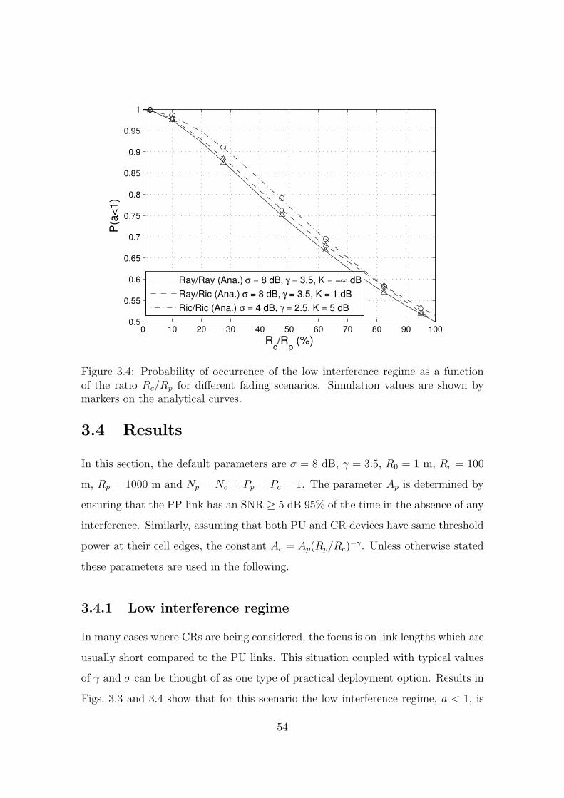
0 10 20 30 40 50 60 70 80 90 1000.5
0.55
0.6
0.65
0.7
0.75
0.8
0.85
0.9
0.95
1
Rc/R
p (%)
P(a
<1
)
Ray/Ray (Ana.) σ = 8 dB, γ = 3.5, K = −∞ dB
Ray/Ric (Ana.) σ = 8 dB, γ = 3.5, K = 1 dB
Ric/Ric (Ana.) σ = 4 dB, γ = 2.5, K = 5 dB
Figure 3.4: Probability of occurrence of the low interference regime as a functionof the ratio Rc/Rp for different fading scenarios. Simulation values are shown bymarkers on the analytical curves.
3.4 Results
In this section, the default parameters are σ = 8 dB, γ = 3.5, R0 = 1 m, Rc = 100
m, Rp = 1000 m and Np = Nc = Pp = Pc = 1. The parameter Ap is determined by
ensuring that the PP link has an SNR ≥ 5 dB 95% of the time in the absence of any
interference. Similarly, assuming that both PU and CR devices have same threshold
power at their cell edges, the constant Ac = Ap(Rp/Rc)−γ. Unless otherwise stated
these parameters are used in the following.
3.4.1 Low interference regime
In many cases where CRs are being considered, the focus is on link lengths which are
usually short compared to the PU links. This situation coupled with typical values
of γ and σ can be thought of as one type of practical deployment option. Results in
Figs. 3.3 and 3.4 show that for this scenario the low interference regime, a < 1, is
54

−12 −10 −8 −6 −4 −2 00
0.05
0.1
0.15
0.2
0.25
0.3
0.35
0.4
log10
(x)
Pro
ba
bili
ty
Sim. (α) (Ric/Ric)
Sim. (α^
) (Ric/Ric)
Sim. (α) (Ray/Ray)
Sim. (α^
) (Ray/Ray)
Figure 3.5: PDFs of log10(α) and its approximation log10(α). We have representedα and α by a dummy variable x. We use the default parameters for the Ray/Raycurve, whereas, for Ric/Ric we have taken σ = 4 dB, γ = 2.5 and Kr = 5 dB.α represents the exact expression given in (3.6), while α refers to its conditionalapproximation discussed in Sec. 3.3.
dominant. For typical values of γ ∈ [3, 4] and σ ∈ [6, 12] dB we find that P (a < 1)
is usually well over 90% when Rc is less than 20% of Rp. As expected, when Rc
approaches Rp the probability drops and reaches P (a < 1) = 0.5 when Rc = Rp.
Note that this is only the case when all the channel parameters are the same for
the CC and CP links. From Fig. 3.4 we observe that the results are reasonably
insensitive to the type of fast fading. This is due to the lesser importance of the
fast fading compared to the large effects of shadowing and path loss. Figure 3.3 also
verifies the analytical result in (3.15).
The relationship between P (a < 1) and the system parameters is easily seen from
(3.4) which contains the term(rcc/rcp
)γ/2exp
((Xcp − Xcc)/2
). When Rc << Rp,
this term decreases dramatically as γ increases (i.e., P (a < 1) increases) and as
σ increases the term increases (hence P (a < 1) decreases). Also, as Rc increases
rcc/rcp tends to increase which in turn decreases P (a < 1). When Rc ≈ Rp the
low and high interference scenarios occur with similar frequency (Fig. 3.4). This
55

0 5 10 15 20 25 300
0.05
0.1
0.15
0.2
0.25
0.3
0.35
Rc/R
p (%)
E(α
)
(Ray/Ray) σ = 8 dB, γ = 3.5, K = −∞ dB
(Ray/Ray) σ = 8 dB, γ = 3.0, K = −∞ dB
(Ric/Ric) σ = 4.0 dB, γ = 2.5, K = 1 dB
(Ric/Ric) σ = 4.0 dB, γ = 2.5, K = 5 dB
Figure 3.6: Mean value of the power loss parameter, α, as a function of the ratio Rc
Rp
for different fading scenarios.
may be a relevant system consideration if CRs were to be introduced in cellular
bands where the cellular hot spots, indoor micro-cells and CRs will have roughly
the same coverage radius. Note that a is independent of the transmit power, Pc.
These conclusions are all verified in Figs. 3.3 and 3.4.
3.4.2 Statistics of the power loss parameter, α
Figures 3.5-3.7 all focus on the properties of α. Figure 3.5 shows that the probability
density function (PDF) of α is extremely well approximated by the PDF of α in
both Rayleigh and Rician fading channels. In Fig. 3.6 we see that E[α] increases
with increasing values of Rc/Rp and decreasing values of γ. This can be seen from
(3.22) where αapprox contains a (rpprcp)−γ term which increases as γ decreases, thus
increasing the mean value of α. The increase of E[α] with Rc follows from the
corresponding increase in Pc to cater for larger Rc values. Increasing the line of
sight (LOS) factor tends to increase E[α] although the effect is minor compared to
56

−6 −5 −4 −3 −2 −1 00
0.1
0.2
0.3
0.4
0.5
0.6
0.7
0.8
0.9
1
log10
(x)
CD
F(x
)
Analysis (α^ )
Simulation (α)
Figure 3.7: Comparison of the exact and analytical CDFs of the power loss factoron a logarithmic scale for fixed link gains. α represents the exact expression given in(3.6), while α refers to its conditional approximation discussed in Sec. 3.3. Resultsare shown for 5 drops for the case of Ray/Ray fading.
changes in γ, σ or Rc/Rp. In Fig. 3.6 we have limited Rc/Rp to a maximum of 30%
as beyond this value the high interference regime is also present with a non-negligible
probability. In Fig. 3.7 we see the analytical CDF in (3.26) verified by simulations
for five different scenarios of fixed link gains (simply the first five simulated values
of Γpp and Γcp). Note that in the different curves each correspond to a random drop
of the PU and CR transmitters. This fixes the distance and shadow fading terms
in the link gains in (3.2), thereby the remaining variation in (3.1) is only Rayleigh.
By computing a large number of such CDFs and averaging them over the link gains
a single CDF can be constructed. This approach can be used to find the PDF of α
as shown in Fig. 3.5. Note that the curves in Fig. 3.7 do not match exactly since
the analysis is for α and the simulation is for α.
57

−8 −6 −4 −2 0 210
−5
10−4
10−3
10−2
10−1
100
log10
(RCR
)
CD
F
RCR
with exact α (σ = 10 dB γ = 3.5)
RCR
with approximate α^ (σ = 10 dB γ = 3.5)
RCR
with exact α (σ = 8 dB γ = 3.5)
RCR
with approximate α^ (σ = 8 dB γ = 3.5)
Figure 3.8: CDF of the CR rates with the exact α (3.6) and the approximate α(Sec. 3.3) for Ray/Ray fading.
3.4.3 CR rates
Figures 3.8-3.10 focus on the CR rate RCR. Figure 3.8 demonstrates that the use of
α is not only accurate for α but also leads to excellent agreement for the CR rate,
RCR. This agreement holds over the whole range and for all typical parameter values.
Figure 3.9 shows the % loss given by [RCR(α = 0)− RCR(α)]/[RCR(α = 0)]%. We
call it mean loss in the figure since we average over several realizations of channels
involved. We note that we term this quantity as loss in the CR rates since α = 0
corresponds to the CR devoting no power for PU purposes and any non zero value
of this parameter incurs are loss in the rates of the CR. The loss decreases as γ
increases, as discussed above, and increases with σ. From (3.22) it is clear that
increasing σ lends to larger values of exp(Xpp + Xcp) which in turn increases α and
the rate loss. Note that the rate loss is minor for σ ∈ [8−10] dB with Rc = Rp/10. In
chapter 5, we show that the interference to the PU increases with σ and decreases
58

3 3.1 3.2 3.3 3.4 3.5 3.6 3.7 3.8 3.9 40
0.5
1
1.5
2
2.5
3
3.5
Path Loss Exponent, γ
Me
an
Va
lue
of
CR
Ra
te L
oss (
%)
(Ray/Ray) σ = 8 dB, K = −∞ dB
(Ray/Ric) σ = 8 dB, K = 1 dB
(Ric/Ric) σ = 4 dB, K = 5 dB
Figure 3.9: Mean value of the CR rate loss as a function of γ for different fadingconditions. With slight abuse of notation, we take Kr = K in the legend of abovefigure.
with γ. These results reinforce this observation, i.e., when the PU suffers more
interference (σ is larger) the CR has to devote a higher part of its power to the PU.
Consequently the percentage rate loss is higher. Again the effect of Kr, the LOS
factor, is minor compared to that of γ and σ.
Finally, in Fig. 3.10 we investigate the gains available to the CR through in-
creasing transmit power. The original transmit power, Pc, is scaled by the power
inflation factor, β, and the mean CR rate is simulated over a range of β values. Due
to the relaying performed by the CR, the PU rate is unaffected by the CR for any
values of β and so the CR is able to boost its own rate with higher transmit power.
Clearly the increased value of α for higher values of β is outweighed by the larger
Pc value and so the CR does achieve an overall rate gain. In a very coarse way these
results suggest that multiple CRs may be able to co-exist with the PU since the
increased interference power might be due to several CRs and the rate gain might
be spread over several CRs. Of course, this conclusion is speculative as the analysis
59

0 5 10 15 200
0.5
1
1.5
2
2.5
3
Power Inflation Factor, β
Me
an
CR
Ra
te
σ = 8 dB γ = 3.5
σ = 10 dB γ = 3.5
σ = 12 dB γ = 3.5
Figure 3.10: Variation of the mean CR rate with the power inflation factor, β forRay/Ray fading case.
is only valid for a single CR.
3.5 Summary
In this chapter we derive the probability that the “low interference regime” holds
and demonstrate the conditions under which this is the dominant scenario. We
show that the probability of the low interference regime is significantly influenced
by the system geometry. When the CR coverage radius is small relative to the PU
radius, the low interference regime is dominant. On the other hand, when the CR
coverage radius approaches a value similar to the PU coverage radius, the low and
high interference regimes both occur with roughly equal probability. In addition, we
have derived a simple, accurate approximation to α which gives considerable insight
into the system capacity. The α approximation shows that the mean value of α is
increased by small values of γ, large CR coverage zones and higher σ values. This
in turn decreases CR rates due to small values of γ, large CR coverage zones and
60

σ. The effect of the LOS strength is shown to be minor and all results appear to
be insensitive to the type of fast fading. Finally, we have shown that the CR can
increase its own rate with higher transmit powers, although the relationship is only
slowly increasing as expected.
61

62

Chapter 4
Interference and Level Crossing
Statistics
We know from the discussion in earlier chapters that the CRs should try their best
to protect the PUs from adverse interference. However, such efforts may jeopardize
the quality of service (QoS) expected from the cognitive devices. Accurate spectrum
sensing capabilities are being developed [8] for CRs and it is envisaged that either
individually, or via collaboration, the cognitive devices will be able to detect the
licensed users with an acceptably low probability of failure. It is evident that the
statistics of the interfering signals will play an important role in the design of CR
systems. Thus, modeling the total CR interference is an important issue and it is
necessary to characterize the nature of the interfering signals along with their impact
on the performance of the incumbent licensed users. Various results [61, 62] have
appeared in this regard. [62] models the combined interference with heavy-tailed
α1-stable distributions in an infinite field of interferers. [61] proposes a 3-parameter
lognormal to accomplish this task. Later in the chapter we show that this approach
is applicable only in certain scenarios.
While devising various CR scheduling strategies it is normal to consider an av-
erage interference constraint [63]. For example, the approaches in [64, 65, 63] allow
1This α should not be confused with the α used in Chapter 3 to represent the power lossparameter in the CR channel.
63

CRs to operate on the basis of average interference powers or SINR values and do
not consider the instantaneous temporal variation of the interference. It is quite
possible that an apparently plausible allocation strategy may result in the CR inter-
ference crossing a particular threshold on too many occasions when the interference
process is considered over time. Thus the motivation to study the LCR of cumulative
interference in conjunction with a particular CR allocation policy.
In this regard our contributions include the following. We derive the CDF of
the interference due to a cognitive device assuming lognormal shadowing and path
loss effects and investigate the nature of the distribution of the total interference
due to multiple CRs. We derive a simplified expression for the cumulants of the
total interference, which are in turn used in approximating the interference with a
shifted lognormal distribution and determining the scenarios of applicability of this
approach. Then, we compute the LCRs of the cumulative interference created by
the CRs. We derive analytical formulae for the LCRs in Rayleigh and Rician fast
fading conditions. We approximate Rayleigh and Rician LCRs using fluctuation
rates of gamma and scaled noncentral χ2 processes, respectively. The analytical
results and the approximations used in their derivations are verified by Monte Carlo
simulations and the analysis is applied to a particular CR allocation strategy.
4.1 System Model
In the system model we consider a PU receiver in the center of a circular region of
radius R. The PU transmitter is located uniformly in an annulus of outer radius R
and inner radius R0 centered on the PU receiver. It is to be noted that we place the
PU receiver at the center only for the sake of mathematical convenience (see Fig.
4.1). The use of the annulus restricts devices from being too close to the receiver.
As seen in Chapter 3, this matches physical reality and also avoids problems with
the classical inverse power law relationship between signal strength and distance
[10]. In particular, having a minimum distance, R0, prevents the signal strength
from becoming infinite as the transmitter approaches the receiver. Similarly, we
64

Re
RCR
CR
PRIMARYTRASMITTER
CR
CR
PRIMARYRECEIVER
CR
CR
Figure 4.1: System model (R0 not shown)
assume that multiple CR transmitters are uniformly located in the annulus. At any
given time, each CR has a probability of seeking a connection, given by the activity
factor, p. The number of CRs wishing to operate is denoted NCR. Of these CRs, a
certain number will be accepted depending on the allocation mechanism. Hence, a
random number of CRs denoted N ≤ NCR will transmit during the PU transmission
and create interference at the PU receiver. The received signal strength for both
the PU transmitter to PU receiver and CR transmitter to PU receiver is assumed to
follow the classical distance dependent, lognormal shadowing model. For a generic
interferer, this is given by
I = BLr−γ = B10X/10r−γ = BeXr−γ, (4.1)
where r is the random distance from the transmitter to the receiver, γ is the path
loss exponent (normally in the range of 2 to 4) and L is a shadow fading variable.
The lognormal variable, L, is given in terms of the zero mean Gaussian, X, which
has standard deviation σ (dB) and X = βX where β = ln(10)/10. The standard
deviation of X is denoted by σsf . The constant B is determined by the methods
discussed in Chapters 2 and 3. The desired primary signal strength, S, has the same
65

form, with a different transmit power, so that S = ALpr−γp . Note that all the links
are assumed to be i.i.d. and spatial correlation is ignored.
4.2 Statistical Characterization of Interference at
the Primary Receiver
4.2.1 Interference Due to a Single Cognitive User
In this section we investigate the interference at the PU receiver due to one or more
CRs. Firstly we characterize the interfering signal, given in (4.1), by computing the
CDF, FI(x) = P (I < x). This can be done as follows
FI(x) = P(BeXr−γ < x
)= P
(e−Xrγ >
B
x
)
= P (eUrγ > y) = EU
[P(r > y
1γ e
−Uγ
)]
= EU
[1− FR
(y
1γ e
−Uγ
)]. (4.2)
In (4.2), U = −X, EU [.] represents expectation over the random variable U and
y = B/x. To evaluate the expectation in (4.2) we note that the CDF of r is given
by
FR(r) =r2 − R2
0
R2 − R20
, R0 ≤ r ≤ R. (4.3)
Using this CDF, (4.2) can be rewritten as
FI(x) = EU [GR(U, y)], (4.4)
where
GR(U, y) =
0 U < w0(R2−y
2γ e
−2uγ
R2−R20
)w0 < U < w1
1 U > w1,
(4.5)
and w0 = ln(yR−γ), w1 = ln(yR−γ0 ). Since U = −X is Gaussian, U ∼ N (0, σ2
sf),
with probability density function (PDF) f(u), the CDF, FI(x) = EU [GR(U, y)],
66

becomes
FI(x) =
∫ w1
w0
R2 − y2γ e
−2uγ
R2 − R20
f(u)du +
∫ ∞
w1
f(u)du =R2
(R2 − R20)√
2πσ2sf
∫ w1
w0
e−u2
2σ2sf du
− (Bx)2/γ
(R2 − R20)√
2πσ2sf
∫ w1
w0
e−2u
γ− −u2
2σ2sf du +
1√2πσ2
sf
∫ ∞
w1
e−u2
2σ2sf du. (4.6)
All the integrals in (4.6) can be written in terms of integrals of Gaussian PDFs.
Hence, (4.6) reduces to
FI(x) = 1− FZ
(w1
σsf
)+
1
R2 − R20
[R2FZ
( w1
σsf
)− R2FZ
( w0
σsf
)
−(B
x
) 2γ
e
(2σ2
sf
γ2
)FZ
(w1 + 2σ2
sf/γ
σsf
)− FZ
(w0 + 2σ2
sf/γ
σsf
)], (4.7)
where FZ(.) is the CDF of a standard Gaussian. In order to validate the CDF
given in (4.7), we compare the results of this expression with the complementary
CDF obtained using Monte Carlo simulation as shown in Fig. 4.2. We note that
although these results are expected to match exactly (since we are not approxi-
mating), the tails represent a simulation mismatch on account of fewer simulation
samples. However, if there were any approximating techniques used then it would be
more plausible to include confidence intervals on the graph. It can be seen that the
analytical and simulated interference complementary CDFs agree over a wide range
of propagation parameters. Hence, a complete characterization of the interference
due to a single CR is possible. Next, we consider multiple CRs.
4.2.2 Interference Due to Multiple Cognitive Radios
In cognitive wireless networks the PU device under consideration may be affected
by the interference due to many CRs. In this case, the total interference, denoted
IT , is given by
IT =N∑
i=1
BeXir−γi =
N∑
i=1
BLir−γi , (4.8)
where the parameters are as defined in (4.1). Equation (4.8) is a random sum
of a finite number of lognormals with each lognormal being multiplied by a ran-
67

−100 −80 −60 −40 −20 0 20 40 6010
−3
10−2
10−1
100
Interference (dB)
Com
ple
menta
ry C
DF
σ = 8.0 dB
γ = 3.0
σ = 6.5 dB
γ = 3.5
σ = 10.0 dB
γ = 4.0
Figure 4.2: A comparison of analytical and simulated complementary CDFs of in-terference over a range of propagation parameters. Solid lines represent analyticalresults while dotted-dashed curves show simulated values.
dom distance factor. Problems similar to this, but involving a non random sum
without incorporating the random distance factor, have been tackled in the past
[66, 67, 68, 69, 70, 71, 72]. Historically, lognormal approximations to this summation
have been envisaged. Approximations are definitely required since although (4.7)
gives an analytical result for a single interferer, it is too complex to allow an exact
approach for sums of interferers. Hence, one is tempted to use the same lognormal
approximation for (4.8). However, as described below, we show that lognormal ap-
proximations are not accurate. We note that instead of showing discrepancy of the
traditional approaches by displaying mismatch between the simulation and analyti-
cal results, we rely on mathematical analysis based on the shape determining factor
of skewness. For convenience, consider a lognormal approximation to a single inter-
ferer, I, of the form given in (4.1). Let the moments of I be denoted by E[Ij ] = mj .
We seek to approximate I with the lognormal Y = eZ where Z ∼ N (µz, σ2z). The
simplest approach to fitting Y is via the Fenton-Wilkinson approach [66, 68] which
68

computes the first two moments, so that
E[Y k] = E[Ik] = mk, k = 1, 2. (4.9)
Hence, the lognormal approximation has perfect moments up to order 2. To demon-
strate the lack of fit we consider the skewness of Y and I which also involves the
third moment. For any lognormal, say Y , the third moment is related to the first
two by
E[Y 3] =
(E[Y 2]
E[Y ]
)3
. (4.10)
Now, consider the skewness of I,
SK(I) =E[(I −m1)
3]
(m2 −m21)
3/2
=m3 + 2m3
1 − 3m1m2
(m2 −m21)
3/2. (4.11)
Similarly, the skewness of Y can be written as
SK(Y ) =E[Y 3] + 2E[Y ]3 − 3E[Y ]E[Y 2]
(E[Y 2]− E[Y ]2)3/2
=E[Y 3] + 2m3
1 − 3m1m2
(m2 −m21)
3/2. (4.12)
Hence, the lognormal approximation is more skewed than the real interference if
E[Y 3] > m3. Now, consider
E[Y 3]
m3
=(m2/m1)
3
m3
=
(B2
E[e2X ]E[r−2γ ]BE[eX ]E[r−γ ]
)3
B3E[e3X ]E[r−3γ ]
=
(E[e2X ]E[eX ]
)3
E[e3X ]
(E[r−2γ ]E[r−γ ]
)3
E[r−3γ]=
(E[r−2γ ]E[r−γ ]
)3
E[r−3γ ]. (4.13)
The above results follow since (4.10) also holds for the lognormal eX . The moments
of r in (4.13) can be found as
E[r−kγ] =2(R2−kγ −R2−kγ
0 )
(R2 − R20)(2− kγ)
. (4.14)
69

Equation (4.14) is obtained using (4.3) as the CDF of r to compute the PDF and
hence the moments. For large R (1000 m in our case), small R0 (we use 1 m) and
with γ ≥ 3, (4.14) gives
E[r−kγ] ≈ −1
R2
(2
2− kγ
)=
2
R2(kγ − 2). (4.15)
Thus, the ratio of the moments in (4.13) becomes:
E[Y 3]
m3≈(
γ − 2
2γ − 2
)3R2(3γ − 2)
2. (4.16)
It can be observed from the above expression that for typical values of the pa-
rameters, E[Y 3] >> m3, and the ratio is of the order of R2. Thus the equivalent
lognormal will be massively more skewed than the real interference. As skewness
is a key shape determining factor (especially in the tails), the simple lognormal ap-
proximation will not be accurate. Note that this large discrepancy in skewness is
due to the random distance factors. Exactly the same conclusions are reached when
attempting to fit sums of interferers. Hence, it appears that a simple lognormal ap-
proximation will not suffice and further research is required. An alternate approach,
one considered by [61], is to approximate interference of the form given in (4.8) with
a three parameter lognormal random variable using cumulant matching. Such an
approximation was shown to be highly accurate under typical operating conditions
of the system considered in [61]. The parameters of the distribution can be expressed
in terms of the cumulants of the interference which is now denoted IT,N to represent
the dependence on the random number of interferers, N . For the sake of analytical
tractability, instead of using a binomial random variable to model the interfering
CRs, we use a Poisson random variable noting that the Poisson distribution is a
limiting case of the binomial. These cumulants can be calculated by modeling the
interferers by a marked Poisson process and invoking Campbell’s theorem [73]. In
what follows we provide a significantly simplified and more intuitive method of cal-
culating the cumulants of IT,N than the one presented in [61]. We begin by noting
that the moment generating function (MGF) of IT,N can be expressed as a function
70

of the MGF of I by means of conditioning on N . Hence,
ΦIT,N(s) = E[esIT,N ]
=∞∑
n=0
E[esIT,N |N = n]P (N = n)
=
∞∑
n=0
E[esIT,n ]P (N = n)
=
∞∑
n=0
(ΦI(s))n P (N = n), (4.17)
where the last equality assumes i.i.d. interferers. We recognize that (4.17) is in the
form of the probability generating function (PGF) of N , and thus
ΦIT,N(s) = GN (ΦI(s)) , (4.18)
where the PGF, GN , for a Poisson distributed N with mean λ is given by
GN(s) = eλ(s−1). (4.19)
Before proceeding forward, we make an important remark. Using (4.19) one may be
tempted to obtain the exact distribution of the cumulative interference. For exam-
ple, it is plain to see that the characteristic function2 of this variable is ΦIT,N(jt) =
exp
(λ(ΦI(jt)− 1)
), where j =
√−1. Further, the characteristic function of the
individual interferer is given by
ΦI(jt) = E[ejtBeXr−γ
] =
∫ R
R0
∫ ∞
−∞ejtBexr−γ
f(x)fR(r)dxdr, (4.20)
where f(x) is the PDF of a N (0, σ2sf) variable and fR(r) can be obtained by differ-
entiating (4.3). With the CDF given in (4.7), it is easy to see that (4.20) may not
be representable in terms of elementary functions or may not even allow a closed
form solution. On top of this, evaluating the inverse Fourier transform of ΦIT,N(jt)
may be a very difficult, if not an impossible, task. Thus the motivation behind
fitting a simple distribution. We note that some progress is possible using stable
2We use characteristics function since this function always exists even when it is not possibleto evaluate the MGF.
71

distributions [62] but this requires the assumptions that R0 → 0 and R→∞ giving
rise to an infinite field of interferers.
Coming back to (4.19), we see that using (4.18) and (4.19) we can obtain the
kth cumulant κk of IT,N as
κk =
[∂k
∂skln ΦIT,N
(s)
]
s=0
= λ
[∂k
∂skΦI(s)
]
s=0
= λE[Ik]. (4.21)
Thus, the cumulants of the aggregate interference can be easily obtained from the
moments of the individual interferers.3 Using (4.1), (4.14) and the moments of a
lognormal the cumulants in (4.21) can be given as
κk = λBkek2σ2sf
/2
(2
2− kγ
)(R2−kγ − R2−kγ
0
R2 − R20
). (4.22)
Following [61] a shifted lognormal was fitted to the interference, IT,N , by selecting
the three parameters of the shifted lognormal to match the first 3 cumulants in
(4.22). Although the fitting procedure was successful, the resulting shift parameter
was found to be negative. Hence, in order to match the first 3 moments of IT,N
the shifted lognormal yields negative interference values for some portion of the
time. Investigation of this behavior showed that the negative shift is fundamentally
a function of R0. For one set of parameter settings, R = 1000 m, σ = 8 dB,
γ = 3.5 and λ = 1000 CRs per square kilometer with an activity factor of 0.1, the
percentage of the shifted lognormal distribution which is negative is given in Table
6.1. From Table 6.1 it is clear that for small R0 values the shifted lognormal is
completely inappropriate as a model for interference. However, for R0 ≥ 20 m the
distribution is always positive and in this region it may be useful. Note that in [61]
a high detection probability near the PU receiver’s beacon means that CRs are very
unlikely to be close to the PU. This is roughly equivalent to a larger R0 value and
3The same result can be obtained via Campbell’s theorem [73], as considered by [61], by ap-propriately modifying the expression for finite cell radius and disregarding the sensing-relatedcomponent.
72

Table 4.1: The percentage of the shifted lognormal distribution which is negativefor various R0 values.
R0 (m) %
1.0 88%
10 72%
16 50%
20 0%
hence in the presence of a beacon the shifted lognormal may be useful as shown in
[61]. However, in this work we are not necessarily assuming a beacon is present and
so the shifted lognormal is not used.
4.3 Level Crossing Analysis
We observed in Chapter 2 that instantaneous variations in signal level are impor-
tant from the perspective of designing and analyzing the performance of wireless
communication systems. In the same way, small scale variations in the composite
CR interference can degrade the PU performance even though the CR levels may be
acceptable on average. Thus, the determination of the rate at which the instanta-
neous interference crosses a particular threshold and the duration for which it stays
above or below it, is an issue of core importance. For example, the PU system may
set an average interference constraint but if the interference exceeds this threshold
for too long or crosses it too often for satisfactory QoS then the threshold may need
to be reduced. From the perspective of CR system design, such an analysis can
provide insight into issues such as CR allocation and power control. For example,
how should the powers of CR devices be controlled keeping in mind the instanta-
neous fluctuations of the interfering signals at the PU receiver? Thus throughout
the remaining part of this chapter SNR or SINR values represent long term average
values while the interference is considered on an instantaneous scale.
73

4.4 Instantaneous CR performance
In any CR allocation policy, for example chapter 5, even if the target interfer-
ence/SINR of the PU is exactly met, the fast fading will result in fluctuations of the
instantaneous interference/SINR both above and below the target. As a first look at
this problem we fix the PU signal power and consider the instantaneous variation of
the interference only. Hence, in this section we focus on the instantaneous temporal
behavior of the aggregate interference via the LCR.
4.4.1 LCRs for Rayleigh Fading
For a given set of CR interferers, the instantaneous aggregate interference, IRay(t),
is given by
IRay(t) =
N∑
i=1
Ii|hi(t)|2, (4.23)
where Ii represents the long term interference power of the ith CR, hi(t) is the cor-
responding normalized channel gain so that in Rayleigh fading |hi(t)|2 is a standard
exponential random variable with unit mean and N is the number of interfering
CRs. Note that we fix the long term interference values, I1, . . . , IN and consider
the variation of the fast fading terms, hi. From (4.23), the aggregate interference is
represented as a weighted sum of exponential variables. Such weighted sums can be
approximated by a gamma variable [60]. The corresponding LCR results are shown
to be accurate in Figs. 4.3-4.5, hence, justifying the approximation of cumulative
interference in (4.23) by a gamma variable. Note that the exact LCR computation
for such sums was given in [74] for the case of three and four branch maximal ratio
combining (MRC) by providing special function integrals. Recently, more general
expressions for arbitrary number of branches have been derived in [75]. However, the
approach of [75] may result in numerical difficulties, especially for large values of N ,
which can be the case for CR systems. In particular, the hypergeometric functions
in [75] are difficult to compute accurately for large negative arguments which is the
case with weak CR interferers. Hence, an approximation is useful to overcome these
74

problems and to provide a much simpler solution. Thus, approximate LCRs for
(4.23) can be found by approximating using a fitted gamma process. It is important
to note that the following approximation is valid only for 2-D isotropic scattering,
when the time autocorrelation function follows the classic Jakes’ model [9]. The
LCR for a gamma process has been calculated in [76]. Therefore, the LCR of (4.23)
across a threshold, T , is
LCRIRay(T ) =
1
2Γ(r)
√2|R(0)|
π(θT )r−0.5 exp(−θT ), (4.24)
where r = E[IRay(t)]2/V ar(IRay(t)), θ = E[IRay(t)]/V ar(IRay(t)) and R(0) = ρRay(0)
is the second derivative of the autocorrelation function (ACF) of IRay(t) at time lag,
τ = 0. Computation of (4.24) only requires the mean, variance and ACF of the
random process in (4.23). The first two moments of (4.23) are E[IRay(t)] =∑N
i=1 Ii
and V ar(IRay(t)) =∑N
i=1 I2i . To calculate the ACF, note that
hi(t + τ) = ρi(τ)hi(t) +√
(1− ρ2i (τ))ei(t), (4.25)
where ei(t) is independent of hi(t) and statistically identical to hi(t). Assuming
a Jakes’ fading process, ρi(τ) is the zeroth order Bessel function of the first kind,
J0(2πfDiτ) and fDi
is the Doppler frequency of interferer i. Using (4.25) we have
E[IRay(t)IRay(t + τ)]
=
N∑
i,j=1
IiIjE[|hi(t)|2|hj(t + τ)|2]
=
N∑
i6=j
IiIj +
( N∑
i=1
I2i E[|hi(t)|2(ρ2
i (τ)×|hi(t)|2 + (1− ρ2i (τ))|ei(t)|2)]
)
=N∑
i6=j
IiIj +N∑
i=1
I2i +
N∑
i=1
I2i ρ2
i (τ)
=
( N∑
i=1
Ii
)2
+
N∑
i=1
I2i ρ2
i (τ), (4.26)
where in the second to last step above, we have used the fact that cross products
have zero mean and that E[|hi(t)|4] = 2. The ACF of (4.23) is given by
ρRay(τ)=E[IRay(t)IRay(t + τ)]−E[IRay(t)]E[IRay(t + τ)]√
V ar(IRay(t))V ar(IRay(t + τ)), (4.27)
75

and with the relevant substitutions, the ACF becomes
ρRay(τ) =
∑Ni=1 I2
i J20 (2πfDi
τ)∑N
i=1 I2i
. (4.28)
Finally, using the expansion J0(2πfDτ) = 1− π2f 2Dτ 2 + . . ., the second derivative of
the ACF needed to compute the LCR in (4.24) is evaluated as
ρRay(0) = −4π2
∑Ni=1 I2
i f 2Di∑N
i=1 I2i
. (4.29)
To the best of our knowledge the results in (4.28) and (4.29) are new. Hence, the
three parameters, r, θ and R(0), are available and (4.24) gives the approximate
LCR.
4.4.2 LCRs for Rician Fading
The instantaneous aggregate interference, IRic(t), for Ricean fading is given as
IRic(t) =N∑
i=1
Ii|hi(t)|2, (4.30)
where |hi(t)| is Rician, with Rician K-factor denoted by K, and N, I1, I2, . . . , IN
are as defined in (4.23). Hence, IRic(t) is a weighted sum of noncentral chi-square
(χ2) random variables. Note that standard LCR results for Ricians [9, 77] and non-
central χ2 variables [77] cannot be applied directly here. The work in [78] is for a
single Rician and in [77] the LCR applies to the case where I1 = I2 = . . . = IN and
an exact noncentral χ2 arises with integer degrees of freedom (dof). Instead, using
the same approximation philosophy as that used in the Rayleigh case, we propose
approximating (4.30) by a single noncentral χ2. This approach is less well docu-
mented but has appeared in the literature (see [79]). Also note that a scaled, rather
than a standard, noncentral χ2 distribution is required for fitting and the resulting
best-fitting distribution will almost certainly not have integer dof. A noncentral χ2
variable with v > 0 dof, non-centrality parameter λ ≥ 0 and scale parameter α > 0
has the following PDF
p(x) =α
2exp
(−(λ + αx)
2
)(αx
λ
) v−24
I v−22
(√λαx
), x > 0 (4.31)
76

where I(v−2)/2 is a modified Bessel function of the first kind with order (v−2)/2. Fit-
ting the PDF in (4.31) to the variable in (4.30) is performed using the method of mo-
ments technique so that the approximate noncentral χ2 has the same first three mo-
ments as IRic(t). The derivation details are outlined in Appendix C. Note that there
can be numerical difficulties with the approach for certain values of I1, I2, . . . , IN .
These difficulties arise when the parameter values obtained from (C.5) and (C.6) do
not satisfy the constraints v > 0, λ ≥ 0, α > 0. However, when this approach does
not work it is straightforward to perform a numerical minimization of the difference
between the true moments of the CR interference and the moments of the α−scaled
noncentral χ2 variable. Values of λ, v and α which minimize this difference can then
be used. Finally, we note that this approach can easily be extended to the mixed
interferer scenario where some channels are Rayleigh and the Rician channels have
possibly different K factors. To handle this situation the 3 moments m1, m2, and
m3 derived in the Appendix C need to be recalculated for the case of unequal K
values. This calculation is straightforward due to the independence of the channels.
The LCR of a noncentral χ2 process with integer dof can be readily obtained
from [77]. In particular, if we substitute R = T , σ2 = 1, M = v/2, s2 = λ and
fm = fD in [77, Eq. (15)] we get the following expression for the LCR of the
α−scaled noncentral χ2 variable
LCRIRic=√
πfD(αT )v4 λ
−(v−2)4 e
(−λ−αT
2
)I v−2
2
(√λαT
). (4.32)
The result in (4.32) holds good for a noncentral χ2 process with integer dof. As
elaborated in [77, 9], the above approximation holds under a set of conditions con-
cerning Doppler frequencies and angles of arrival. For example, the result is valid
under isotropic scattering when the LOS component has an angle of arrival of π/2
relative to the direction of the motion of mobile. In Appendix D we show that this
formula is also valid for non-integer dof. Note that a similar extension for a central
χ2 with integer order [80] to a central χ2 with fractional order [76] has also been
shown to be correct. We observe that if Ii = I, ∀i (the condition for which (4.24)
holds exactly), then using K = 0 in (C.3) and (C.4) gives λ = 0, α = 2/I and
77

v = 2N as a solution to (C.5) and (C.6). Using these values and the approximation,
Iv(z) ∼ (z/2)v/Γ(v+1) when z → 0, in (4.32), some manipulations show that (4.32)
reduces to the expression in (4.24).
4.4.3 Average Exceedance Duration
We define the AED for both Rayleigh and Rician environments as the average time
that the aggregate interference stays above a given threshold T [9]. Mathematically,
AED =1− F (T )
LCR, (4.33)
where F (T ) gives the distribution function of the aggregate interference. Note that
the exact CDFs of both IRay(t) and IRic(t) can be found in [81]. We note that the
models in (4.23) and (4.30) and the analysis in (4.24), (4.32), (4.33) are valid for
any scenario where interference caused by multiple Rayleigh or Rician interferers is
of interest. Hence, the scope of the contribution is much wider than CR systems.
4.5 Results
In order to evaluate the accuracy of (4.24) and (4.32) it is important to use realistic
values of I1, I2, . . . , IN . Hence, we use a particular CR access scheme chapter 5 to
provide these values. The decentralized selection algorithm in chapter 5 employs a
controller that considers CRs in their order of arrival. Each interferer is considered in
turn and is accepted if the combined interference from previously accepted CRs and
the current CR is less than some interference threshold. If a CR is not accepted,
the next CR in the list is investigated. The Ii values are generated in chapter 5
from randomly located CRs in a circular region and include path loss and shadowing
effects. In chapter 5 a threshold value is used which corresponds to the PU accepting
a 2 dB loss in its SNR due to the presence of CRs.
From 1000 simulations, using the above selection procedure two sets of interfer-
ers were selected. The first set selected had the highest variance. Only 3 CRs were
78

−30 −25 −20 −15 −10 −5 0 5 100
0.2
0.4
0.6
0.8
1
1.2
1.4
10 log10
(κ) (dB)
LC
R/f
D
Rayleigh
Rician (K = 5 dB)
Rician (K = 10 dB)
Figure 4.3: LCR results for different fading conditions with dominant interferers.The solid lines represent analytical results. Simulation values are shown by thecircle, star and triangle symbols.
accepted and there was a dominant interferer which accounted for 95% of the inter-
ference power. The second set had the lowest variance, representing the no dominant
interferer scenario. Here, 18 CRs were accepted with the largest interferer only ac-
counting for 16%. Note that with equal values of I1, I2, . . . , IN the results in (4.24),
(4.32) are exact. Hence, the worst cases for fitting are when the interferers have a
large variance. This is the first scenario. Thus, in addition to giving examples of en-
gineering importance (presence or absence of a dominant interferer) these two cases
also test the general applicability of (4.24) and (4.32) over a wide range of interferer
profiles. These sets were obtained using the following parameter values: shadow
fading standard deviation, σ = 8.0 dB, path loss exponent, γ = 3.5, radius of PU
coverage area, R = 1000 m, radius of CR coverage area, Rc = 100 m, CR density
of 1000 CRs per square kilometer, an activity factor of 0.1 and a common Doppler
frequency of fD = 25 Hz. Coverage areas are defined to be the areas in which the
79

−30 −25 −20 −15 −10 −5 0 5 100
0.2
0.4
0.6
0.8
1
1.2
1.4
10 log10
(κ) (dB)
LC
R/f
D
dominant interferer
no dominant interferer
Figure 4.4: LCR results for the dominant and no dominant interferer cases in aRayleigh fading scenario. The solid lines represent analytical results. Simulationvalues are shown by the circle and star symbols. The interference threshold valuesand their LCRs are shown by dotted lines.
received SINR is greater than a certain threshold at least 95% of time. We simulate
LCRs by generating 105 independent channel pairs for each interferer, where each
pair consists of (hi(t), hi(t+τ)) where hi(t) and hi(t+τ) are correlated according to
the channel ACF which depends on the Doppler frequency. This approach enables
an exact generation of the pairs and a rapid evaluation of LCR. Approaches that
generate a single, long process over time are slower and require approximate models.
LCR and AED of CR-PU Interference
Figures 4.3, 4.4 and 4.5 show the LCR (normalized by Doppler frequency) of the
interference for different types of fading and interference profiles. The x-axis is
also normalized by the rms value of the process so that κ = T/√
m2 is plotted,
80

−14 −12 −10 −8 −6 −4 −2 0 2 4 60
0.1
0.2
0.3
0.4
0.5
0.6
0.7
0.8
0.9
10 log10
(κ) (dB)
LC
R/f
D
dominant interferer
no dominant interferer
Figure 4.5: LCR results for the dominant and no dominant interferer cases in aRician (K = 10 dB) fading scenario. The solid lines represent analytical results.Simulation values are shown by the circle and star symbols. The interference thresh-old values and their LCRs are shown by dotted lines.
where T is the interference power level and m2 is the mean-square interference
(see Appendix C). Figure 4.3 shows the effect on LCR of increasing the Rician
K-factor, with the strong LOS case being considerably narrower than the non-LOS
case. Figures 4.4 and 4.5 also show the value of the normalized interference threshold
that restricts the long term average interference value in the CR system (as shown by
the dotted lines). Note that there are multiple thresholds since the normalization
is different for different channels. For all types of fading, the maximum LCR is
observed close to this threshold value. This is because the CR allocation method
gives a mean interference level close to the threshold. Even in strong LOS conditions
(K = 10 dB), the interference shows a significant number of level crossings across the
buffer due to the scattered component. Figure 4.4 shows the case of Rayleigh fading
where the interference budget is dominated by a single large interferer with a number
81

−20 −15 −10 −5 0 5 1010
−1
100
101
102
103
104
105
10 log10
(κ) (dB)
AE
D×
fD
dominant interferer
no dominant interferer
Figure 4.6: AED results for the dominant and no dominant interferer cases in aRician (K = 10 dB) fading scenario. The solid lines represent analytical results.Simulation values are shown by the circle and star symbols.
of smaller additional interferers. Also shown is the no dominant interferer case.
Figure 4.5 shows the same results for a Rician channel with K = 10 dB. Figures 4.4
and 4.5 show that when there are many small interferers, the interference is more
stable compared to the dominant interferer case. The results in Fig. 4.5 are quite
promising. In near LOS conditions, the interference has a much lower level crossing
rate across the interference buffer for the no dominant interferer case. Hence, it
may be a desirable part of the CR allocation policy to avoid any single user which
takes up a significant part of the buffer. Finally, for completeness, we show the AED
results corresponding to Fig. 4.5 in Fig. 4.6. As expected, the time spent by the
interference above a threshold decreases as the threshold value increases. Therefore,
for the no dominant interferer case, the interference seldom crosses the threshold
(see Fig. 4.5), and when it does, it only exceeds the threshold for a small period of
time. Since the LCR curve for the no dominant case is much sharper in Fig. 4.5,
82

the corresponding AED is much steeper. For example, −2 dB is rarely crossed in
Fig. 4.5 and this corresponds to a very high AED value at the same threshold. All
figures show an excellent agreement between the analytical approximations and the
simulations.
4.6 Summary
In this chapter we have shown that the interference due to a single CR can be char-
acterized in closed form for the scenario considered. However, the total interference
due to multiple CRs is more difficult. Simple lognormal approximations are shown
to be inaccurate and more complex models are required. Then we determine the
LCR and AED for the CR-PU interference for Rayleigh and Rician channels. We
have shown that LCRs in Rayleigh environment can be accurately approximated by
LCRs of a gamma process. Similarly, while deriving LCR approximations in Rician
conditions we have shown that the LCR of a noncentral χ2 process with non-integer
dof has the same form as that of a noncentral χ2 process with integer dof. The
LCR results show that in near LOS conditions, it is desirable for any CR allocation
method to give priority to several small interfering CRs rather than a dominant
interfering CR. The LCR of the former shows a greatly reduced crossing rate at
and above the interference threshold. The AED results also show that the for the
no dominant interferer case, the interference only exceeds the threshold for small
period of time.
83

84

Chapter 5
Cognitive Radio Allocation
Schemes
In addition to sensing techniques, a number of schemes aimed at avoiding harm-
ful interference due to CRs at PUs have recently been developed, either based on a
primary exclusion zone (PEZ) approach [58] or on the exploitation of radio environ-
ment map (REM) [82] information. The former utilizes the knowledge of interference
statistics to define an exclusion zone inside which CRs are not permitted to oper-
ate, while the latter, which assumes a more complete knowledge of the interferers
including their geographical position, permits only selected CRs to operate in order
to maintain a specific SINR.
From our discussion in Chapter 4, it is clear that we cannot approximate the
cumulative CR interference with a simple distribution. The availability of such a
result would have helped in calculating, for example, an exact expression for the
exclusion zone radius in PEZ schemes or the number of allowable CRs in the REM
based techniques. This would have further shed light on the dependence of system
performance on various different parameters. Hence, as a first look at this problem
we study various CR scheduling schemes based on results obtained by computer
simulations. We also stress here that we do not deal with the issue of how the
CRs would communicate with each other and pass on the information about their
85

activity as this is beyond the scope of the current work. This, for example, can
involve the CRs communicating with a controller upon obtaining permission for
using the spectrum. Hence, in this chapter our contributions include analyzing a
PEZ approach that allows access to CRs when the primary device is willing to pay a
price in the form of a reduction in its threshold SNR. We determine the permissible
number of CRs when the REM is a priori known to the CRs and establish how
these numbers vary in different fading environments. In the presence of coarse
REM information we show that when the REM for a given area is discretized then
the total CR interference is significantly underestimated when realistic grid sizes are
considered. We also determine the interaction between shadow fading correlation
and REM grid size and evaluate their impact on interference estimation. Finally, we
determine the scenarios (CR density, fading parameters) under which REM equipped
CR systems outperform PEZ based cognitive wireless systems. To the best of our
knowledge, we present the first comparative study of the PEZ and the proposed REM
schemes with and without perfect REM information in shadowing environments.
In the simulations and results to follow, we assume that CRs are located uni-
formly in the primary coverage area. The number of active CRs, NCR, is binomially
distributed1 with a maximum number of CRs given by πR2DCR, where DCR is the
density of the CRs (number of CRs per m2) and we ignore the negligible hole in
the circle of radius R0. The binomial probability that a CR wishes to transmit is
given by the activity factor, p = 0.1. The primary receiver is at the center of the
coverage area and the primary transmitter is also uniformly located in the primary
coverage area. We consider two fundamentally different schemes for managing the
interference at the PU receiver. The REM approach utilizes complete knowledge of
all the interference values whereas the PEZ approach only uses average information
of all interferers within a certain distance of the PU receiver. There are NCR CR
transmitters which desire a connection. Each of the NCR CRs has an interference
1We mention that to arrive at (4.19) we used a Poisson variable to model the interfering CRs (inthe limiting case when the number of CRs tends to infinity and the probability of each interferingCR is small enough) for the sake of mathematical tractability. Here, without loss of generality, weassume a binomial random variable modeling the finite number of such CRs.
86

power at the primary receiver given by (4.1) and denoted I1, I2, . . . , INCR. Based on
these interference values, the PEZ and REM approaches are described below.
5.1 PEZ Approach
The PEZ approach [58] only uses location information to control the access of CRs.
A simple exclusion zone is created with radius Re around the primary receiver. No
CR is allowed to transmit inside the PEZ and all CRs outside the PEZ are permitted.
The radius, Re, is set so that the cell-edge SINR is degraded by a certain amount.
Specifically, the primary coverage area is defined to give an SNR greater than 5 dB,
95% of the time. By allowing CRs to operate we accept a new SINR target, less
than 5 dB, which is achieved at least 95% of the time.
5.2 REM Approach
The REM approach [82] assumes that I1, I2, . . . , INCR(defined to be same as in the
previous chapter) are known and selects those CRs for transmission which satisfy
an SINR constraint. The constraint chosen is that the added interference must not
decrease the SNR by more than Υ dB. For example, if SNR = 10 dB in the absence
of CRs, then those CRs chosen must give SINR ≥ (10− Υ) dB. Two methods are
chosen for selection, a centralized approach and a decentralized approach.
• Centralized Selection: Here we assume that a centralized controller knows
I1, I2, . . . , INCRinstantaneously and creates a list of the ordered interferers as
I(1) ≤ I(2) ≤ . . . ≤ I(NCR). The first n CRs are selected such that∑n
i=1 I(i) ≤ Υ
dB and∑n+1
i=1 I(i) > Υ dB.
• Decentralized Selection: Here we assume that the CRs are considered in their
original order which can be interpreted as their order of arrival. Each interferer
is considered in turn and is accepted if the combined interference from previously
accepted CRs and the current CR is less than Υ dB. If a CR is not accepted,
87

the next CR in the list is investigated.
The usefulness of REM based techniques hinges around the quality of the informa-
tion available. Thus we discriminate between perfect and imperfect REM informa-
tion in the following.
A Perfect REM
A REM can hold a wide variety of information [83] and it is not clearly understood at
present what constitutes a practical and effective REM. In this work we assume that
the REM contains signal strength data. In a perfect REM the signal strength from
all source coordinates to all destination coordinates is known. With this perfect
REM a CR controller can select those CRs for operation which satisfy a given
interference constraint. The CR controller requires positional information for the
PU and the CRs, and can then use the REM to compute the overall SINR of the
PU where
SINR =S
∑Ni=1 Ii + σ2
. (5.1)
In (5.1), S is the signal strength of the PU, σ2 is the noise power and∑N
i=1 Ii is
the aggregate interference of the N selected CRs. The interference constraint used
is that the CR interference must not reduce the PU SNR by more than Υ = 2 dB.
All results shown in the paper are for a 2 dB buffer. The value of 2 dB was chosen
arbitrarily.
Modeling of REM Imperfections
In practice, it is unrealistic to assume a perfect REM and the REM information
is discretized in the form of a grid of points with grid size, ∆. Hence, the central
controller allocating CRs will formulate its decisions on the basis of REM informa-
tion obtained from the grid points, rather than from exact signal strength data.
Therefore, an interfering signal strength, I, will be estimated as I from the REM.
The estimate is obtained from the grid-to-grid path in the REM which is closest to
the actual signal path.
88

We consider the CR signal strength to be of the form given in (4.1). The REM
predicted signal strength is given by
I = BeX r−γ, (5.2)
where r is the distance between the transmitter and the receiver in the REM grid
and X is correlated with X by
X = ρX +√
1− ρ2E. (5.3)
In (5.3) E is i.i.d. with X. Assuming a distance, di, between the actual and REM
based position of the CR and a distance, dp, between the actual and REM based
location of the PU receiver, the correlation coefficient ρ can be obtained using an
extension of Gudmundson’s model [16] as
ρ = 0.5di/Dd × 0.5dp/Dd. (5.4)
In (5.4) Dd is the so called decorrelation distance i.e., the distance at which the
correlation between X and X drops to 0.5. The effect of flawed REM information
on the signal strength between the primary transmitter and its receiver can be
modeled using (5.2), (5.3) and (5.4). Simulation results of this model based on
parameter values of a suburban macrocellular environment are given in Section 5.3.
Optimal Interpolation: The above models for REM imperfections allow the ef-
fects of errors in the REM to be simulated. However, REM accuracy is of key
importance as shown in Sec. 5.3 and hence it is useful to take a closer look at this
issue. In what follows we derive the distribution of the errors resulting from the
imperfect REM under certain idealized conditions.
Consider a REM with grid size, ∆, where the receiver is exactly located at one
grid point and the transmitter location, P , is arbitrary, falling in one square of the
grid pattern. We further assume that the signal strength model in (4.1) is exact
and that, B, r, γ are exactly known. Hence, only the shadow fading is unknown
and this information is exactly known at the grid points. We further assume that
Gudmundson’s model (5.4) holds with dp = 0. Clearly this situation is extremely
89

optimistic and leads to a lower bound on realistic REM errors. Now consider the
signal strength from P to the PU receiver where P falls inside one of the grid boxes.
Since all the five points (the four corners of the box and P ) experience correlated
shadow fading, we model the correlation between the normal random variables, Xi,
associated with the lognormal shadowing at the five points using Gudmundson’s
model [16]. Thus,
ρ(Xi, Xj) = adij , i, j = 1, . . . , 5, (5.5)
where ρ(Xi, Xj) represents the corrrelation between Xi and Xj , and dij is the dis-
tance between Xi and Xj. Using Gudmundson’s results we choose a = 0.998 for
suburban environments and a = 0.886 for urban environments. Furthermore, we
assume that X1 to X4 form the corner points of the square with the principal di-
agonal between X1 and X3 and the other diagonal between X2 and X4. Hence, we
have the following correlation matrix for (X1, . . . , X5)T :
R =
1 r r√
2 r rd1
r 1 r r√
2 rd2
r√
2 r 1 r rd3
r r√
2 r 1 rd4
rd1 rd2 rd3 rd4 1
, (5.6)
where r = a∆, ρ(X5, Xi) = adi∆ = rdi, ∀i and di is the distance from the point P
to the ith corner of the square. Performing the Cholesky decomposition we have
R = AA†, where A is a lower triangular matrix. Clearly, A can be factored as,
A =
A11 0
aT b
, (5.7)
where A11, 0 and aT represent a sub-matrix, a column vector of zeros and a row
vector of appropriate sizes, respectively. Further, b represents a scalar lying between
90

0 and 1. With this notation, it can be shown that,
X5 = aT A−111
X1
X2
X3
X4
+ bu5, (5.8)
where u5 is N (0, σ2sf). The first term in (5.8) represents the optimal estimator of X5
using the REM and the second term gives the estimation error which is N (0, b2σ2sf).
Note that this is standard theory [84]. Further it is worth emphasizing that this
analysis can easily be extended to interpolation using more than 4 REM grid values.
It is evident that the performance of the above scheme heavily depends on the
behavior of the error term which in turn relies on ∆ and σsf . One way to evaluate
this is to compute the probability of underestimating signal strength (interference)
from the CR devices. Based on (5.5)-(5.8) the probability of underestimating the
interfering signal strength by an amount, E, is given by
PE = Probability of underestimating the signal strength by more than E dB
= P (estimation error < −E dB) = Q
(E
bσ
), (5.9)
where Q(.) gives the tail probability of a standard Gaussian. Hence, the Cholesky
decomposition of R gives b which directly leads to (5.9), a simple closed form result
for the effects of imperfect REM.
5.3 Simulation Results
Unless otherwise stated, we assume a PU coverage radius of R = 1000 m, and the
transmit power is adjusted such that the SNR at the cell edge is 5 dB (i.e., in
the coverage area the SNR exceeds 5 dB with probability 0.95). The CR transmit
power is also chosen to meet a cell edge SNR of 5 dB for a given CR coverage radius,
Rc = 100 m. Two kinds of CR penetration densities were chosen, a high density
of 10, 000 CRs per sq. km and a corresponding moderate density of 1000 CRs per
91

0 0.5 1 1.5 2 2.5 3 3.5 4200
300
400
500
600
700
800
900
1000
Target SINR (dB)
Prim
ary
Exclu
sio
n Z
on
e R
ad
ius (
m)
σ = 8 dB γ = 3.5
σ = 12 dB γ = 3.5
σ = 6 dB γ = 3.5
Figure 5.1: The effect of σ and the target SINR on the PEZ radius for a mediumdensity of CRs.
sq. km. Additionally, it was assumed that only 10% of the CRs wish to be active
at any one time. The values of the propagation constants, γ and σ are given on
the relevant figures. The shadow fading variance and path loss exponent should be
taken as 8 dB and 3.5, respectively, when they are not explicitly mentioned.
5.3.1 Exclusion Zone Results
Given a variety of target SINRs, Fig. 5.1 shows the PEZ radius for different values
of σ. For example, if the interference degrades the target SNR from 5 dB to an SINR
of 4 dB, then the PEZ radius is approximately 700 m, for σ = 6 dB and γ = 3.5. It
is interesting to note that the PEZ radius excludes virtually the entire PU coverage
area for all target SINRs in [0, 5] dB when σ = 12 dB, corresponding to dense urban
areas. This result implies that for a given target SINR, environments with larger σ
will result in higher interference and an increased Re. This observation is consistent
with previous observations reported in [85].
92

0 0.5 1 1.5 2 2.5 3 3.5 40
100
200
300
400
500
600
700
800
900
Target SINR (dB)
Prim
ary
Exclu
sio
n Z
on
e R
ad
ius (
m)
R/Rc = 10
R/Rc = 20
R/Rc = 100
Figure 5.2: PEZ radius vs target SINR for different values of the ratio of primaryto secondary device coverage areas (σ = 8 dB, γ = 3.5).
Increasing the CR transmit power or increasing Rc will correspondingly increase
the interference and hence the PEZ radius. Figure 5.2 shows the PEZ radius vs
target SINR for three different values of R/Rc. Reducing the CR transmit power
will obviously result in a lower PEZ radius.
5.3.2 Comparison of Numbers of CRs
Figures 5.3 and 5.4 show CDFs of the number of CRs for the two different types
of REM approach and the impact of varying the fading parameters. In both these
figures, the centralized approach is superior, since it is designed to pick up the
maximum number of CRs that aggregate to make up the acceptable interference
degradation. We also note from Fig. 5.3 that increasing γ increases the number
of permissible CRs. This is because environments where γ = 4 will experience less
interference compared to environments where γ = 3 due to increased path loss.
Looking at Fig. 5.4, increasing σ decreases the permissible number of CRs. This
93
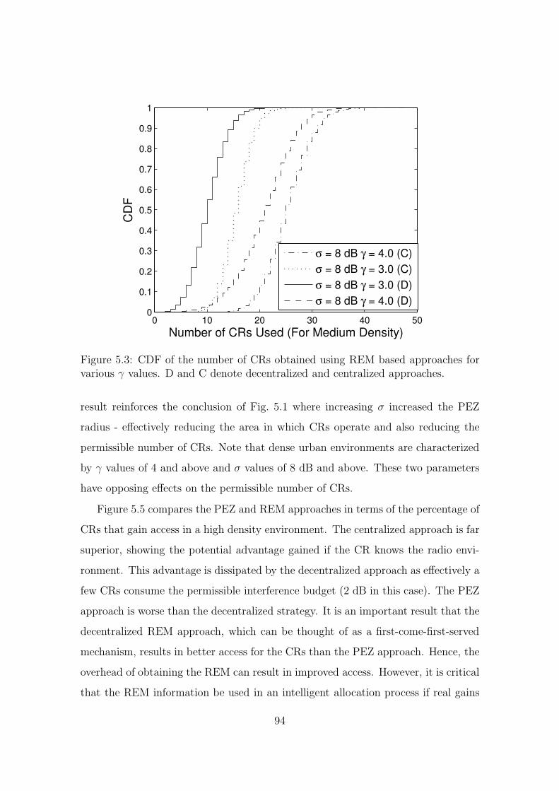
0 10 20 30 40 500
0.1
0.2
0.3
0.4
0.5
0.6
0.7
0.8
0.9
1
Number of CRs Used (For Medium Density)
CD
F
σ = 8 dB γ = 4.0 (C)
σ = 8 dB γ = 3.0 (C)
σ = 8 dB γ = 3.0 (D)
σ = 8 dB γ = 4.0 (D)
Figure 5.3: CDF of the number of CRs obtained using REM based approaches forvarious γ values. D and C denote decentralized and centralized approaches.
result reinforces the conclusion of Fig. 5.1 where increasing σ increased the PEZ
radius - effectively reducing the area in which CRs operate and also reducing the
permissible number of CRs. Note that dense urban environments are characterized
by γ values of 4 and above and σ values of 8 dB and above. These two parameters
have opposing effects on the permissible number of CRs.
Figure 5.5 compares the PEZ and REM approaches in terms of the percentage of
CRs that gain access in a high density environment. The centralized approach is far
superior, showing the potential advantage gained if the CR knows the radio envi-
ronment. This advantage is dissipated by the decentralized approach as effectively a
few CRs consume the permissible interference budget (2 dB in this case). The PEZ
approach is worse than the decentralized strategy. It is an important result that the
decentralized REM approach, which can be thought of as a first-come-first-served
mechanism, results in better access for the CRs than the PEZ approach. Hence, the
overhead of obtaining the REM can result in improved access. However, it is critical
that the REM information be used in an intelligent allocation process if real gains
94

0 5 10 15 20 25 30 35 400
0.1
0.2
0.3
0.4
0.5
0.6
0.7
0.8
0.9
1
Number of CRs Used (For Medium Density)
CD
F
σ = 12 dB γ = 3.5 (D)
σ = 8 dB γ = 3.5 (D)
σ = 8 dB γ = 3.5 (C)
σ = 12 dB γ = 3.5 (C)
Figure 5.4: CDF of the number of CRs obtained using REM based approaches forvarious σ values. D and C denote decentralized and centralized approaches.
over PEZ are to be achieved. Figure 5.6 revisits the results in Fig. 5.5 for a lower
CR density. Here too the centralized approach is better, but now the decentralized
approach shows an even bigger advantage over the PEZ approach for higher values
of the CDF. In addition to this, we also investigate the case of CRs with different
coverage areas. In particular, we consider a coverage circle with radius uniformly
distributed in [50 m, 150 m]. Such scenarios may correspond to heterogenous CR
systems with application specific coverage zones. Clearly, in this case the mean
value of the number of CRs given access remains nearly the same as before in the
two REM based schemes. However, as expected, the variation in the percentage of
CRs given access tends to increase. We note that the PEZ scheme outperforms the
REM based strategies in Fig. 5.5 by a bigger margin than an Fig. 5.6 on account of
the higher CR density employed in Fig. 5.5.
The results in Figs. 5.3-5.6 taken collectively are the important contributions of
this chapter. They clearly show the advantage in terms of permissible CR numbers
95

0 5 10 15 20 25 30 35 40 450
0.1
0.2
0.3
0.4
0.5
0.6
0.7
0.8
0.9
1
Percentage of CRs Used (High CR Density)
CD
F
REM 2 dB (C)
REM 2 dB (D)
PEZ based
Figure 5.5: Percentage of CRs given access for a high CR density (σ = 8 dB,γ = 3.5).
if a knowledge of the radio environment is made available to the CRs. Furthermore,
they show that the full REM gains are only obtained if a smart access control
algorithm is used which chooses many CRs with low interference instead of a few
stronger interferers which might subsume the interference budget.
5.3.3 Imperfections in the REM
In practice, the radio environment is often modeled by dividing an area into a regular
grid (typically composed of 100 m × 100 m grid boxes) and assuming that the fading
conditions in any grid box can be approximated by a single point at the center of the
box. For example, drive testing of cellular networks to validate path loss models and
predicted signal coverage follows this approach. Clearly, larger grid sizes result in
errors between measurement and prediction. On the other hand, reducing the grid
size results in a large data overhead. Figure 5.7 shows the CDF of the magnitude of
the actual CR-PU interference when the REM is estimated via a grid size ranging
96

0 20 40 60 80 1000
0.1
0.2
0.3
0.4
0.5
0.6
0.7
0.8
0.9
1
Percentage of CRs Used (Medium CR Density)
CD
F
REM 2 dB (C)
REM 2 dB (D)
REM 2 dB (C), VR
REM 2 dB (D), VR
PEZ
Figure 5.6: Percentage of CRs given access for a medium CR density (σ = 8 dB,γ = 3.5). VR denotes a variable CR radius uniformly distributed between 50 m and150 m.
from 1 m × 1 m to 100 m × 100 m. The REM approach aims to maintain a 2 dB
SINR buffer for the primary, but this is only possible with a perfect REM. When
∆ = 1 m the 2 dB buffer is nearly achieved (exceeded only 13% of time) but for a
grid size of 50 m × 50 m, the interference exceeds 2 dB for approximately 70% of
the time. For a grid size of 100 m × 100 m, 2 dB is exceeded 85% of the time and
5 dB is exceeded 10% of the time. In effect this means that if REM information is
derived from a coarse grid, the buffer size must be increased or the CRs must back
off from the buffer.
The effects of increasing the buffer or backing off the CRs are shown in Figs. 5.8
and 5.9, respectively. In Fig. 5.8 the PU has a target 2 dB buffer but due to the
imperfect REM it will not always be achieved. Hence, an extra buffer is permitted
beyond which the CRs are only allowed, 5% of the time. In Fig. 5.8 this scenario is
97

0 2 4 6 8 100
0.1
0.2
0.3
0.4
0.5
0.6
0.7
0.8
0.9
1
Buffer (dB)
CD
F
∆ = 1 m
∆ = 10 m
∆ = 50 m
∆ = 100 m
Figure 5.7: Interference CDF for an REM enabled CR network for several values of∆ and decorrelation distance, Dd = 100 m.
denoted by the legend, Threshold = (original + extra) dB. The effects of spatially
correlated shadow fading are also considered in Fig. 5.8. Shadow fading is correlated
over any given area and the level of this correlation has a simple effect on the REM
grid size. For highly correlated areas a coarse grid (large ∆) will be acceptable
whereas in areas of low correlation, a fine grid (small ∆) will be required. Figure 5.8
shows the REM grid size vs the decorrelation distance of the shadow fading. For
a given interference degradation (say the buffer value plus an additional 2 dB) a
large decorrelation distance (say 500 m) enables a coarser grid size 130 m × 130 m
relative to a decorrelation distance of 100 m (typical for dense urban areas) when
the grid size is 38 m × 38 m.
In Fig. 5.9 we consider a back off in the CR allocation policy. In order to meet
the nominal 2 dB SINR buffer at least 99% of the time, the CRs have to target a
reduced buffer which is less than 2 dB. Figure 5.9 shows this buffer vs ∆ for various
values of Dd. For a grid size of 25 m × 25 m and a decorrelation distance of 100 m,
the interference buffer is 0.88 dB. Figures 5.8 and 5.9 are instructive in determining
98

100 150 200 250 300 350 400 450 5000
20
40
60
80
100
120
140
Decorrelation Distance, Dd (m)
RE
M G
rid
Siz
e,
∆ (
m)
Threshold = (buffer + 0.5) dB
Threshold = (buffer + 1.0) dB
Threshold = (buffer + 2.0) dB
Figure 5.8: REM grid size, ∆, vs decorrelation distance, Dd, for different thresholdbuffer sizes.
the grid sizes for different radio environments.
To study the effect of linearly interpolating signal strength from the position of a
source point in a REM grid, we simulate the estimation error introduced in Sec. 5.2
for different environments. In particular, we plot the probability of this error being
less than a threshold of −3 dB (i.e., when we underestimate the interference by more
than 3 dB) for urban and suburban environments based on meshes of 4 and 16 points
for shadow fading variances of 6 dB and 12 dB as shown in Fig. 5.10. It is clear from
the figure that linearly interpolating the signal strength using the nearest 16 points
in the REM grid is no better than using the closest 4 grid points. Furthermore, it is
seen that owing to smaller decorrelation distances, finer grid sizes would be needed
in urban environments (a = 0.886). In addition to this, shadowing has a negative
impact on the performance of such REM systems in terms of underestimating the
true interference produced by the CRs. The scale of the underestimation problem
99

0 5 10 15 20 250.8
1
1.2
1.4
1.6
1.8
2
REM Grid Size, ∆ (m)
Buff
er
(dB
)
Dd = 100 m
Dd = 200 m
Dd = 300 m
Figure 5.9: Variation of actual buffer with REM grid size, ∆, for different values ofthe decorrelation distance, Dd.
can be seen from a few examples in Fig. 5.10. In urban environments with 6 dB
shadowing, 30% of time the interference is underestimated by more than 3 dB for
a grid size of 31.6 m. Even with a much smaller 10 m grid this probability is still
greater than 20%. Hence, despite underestimating the real REM errors, it can be
seen that extremely small grid sizes may be needed to avoid harmful interference.
5.4 Summary
In this chapter two interference management approaches have been considered based
on REM and PEZ ideas. The REM approach requires considerable higher overheads
but can perform substantially better than the PEZ one. To achieve these gains an
intelligent allocation method is essential since providing access to CRs on a first-
come-first-served basis can be worse than the PEZ method. However, the PEZ
approach results in large exclusion zones especially for high σ and large Rc values.
We have shown that interference degradation to the PU can be significantly un-
100

0 0.5 1 1.5 2 2.5 30
0.05
0.1
0.15
0.2
0.25
0.3
0.35
0.4
0.45
0.5
log10
(∆)
PE
6 dB
12 dB
Figure 5.10: Variation of the probability of underestimating the interference versusgrid size. Solid lines are for suburban and dotted lines are for urban environments.The lines (solid and dotted) represent 4 point while the points (circles and squares)depict 16 point interpolation.
derestimated if the channel state information needed to estimate interference levels
is derived from a coarse REM. In particular, the probability of interference under-
estimation has been shown to be very high for urban environments. For practical
deployments, this may mean that the PU has to accept a much larger interference
from the CRs or the CRs may need to set a more conservative interference target.
This will reduce the number of CRs allowed.
101

102

Chapter 6
MIMO Cognitive Radios with
Antenna Selection
The concept of MIMO CR systems has triggered significant interest in the research
community [86, 87, 88, 89]. In CR systems, multiple antennas in addition to provid-
ing rate benefits, can also help in enabling interference control at the PU RX [87].
However, along with the gains, comes hardware complexity at the radio front end
owing to the requirement to have costly RF chains (consisting of low noise ampli-
fiers, downconverters and analog-to-digital converters) that scale with the number
of antennas being used. Even more costly is the provision of power amplifiers and
up converters at the transmit end.
It is well known that antenna selection techniques present an elegant solution
to such problems, see, for example, [90, 91, 92] and the references therein. Recent
work in this area includes [93] where transmit antenna selection was considered for
a MISO CR operating in the presence of a SISO PU. In this chapter, we consider
the problem of joint selection of transmit/receive antennas in a MIMO CR system.
The selection procedure aims to maximize the achievable rate of the CR while sat-
isfying any interference constraints due to the PU RX(s) (either equipped with a
single antenna or multiple antennas) operating in the vicinity. The work in [93]
has similarities in that the SINR results in [93] can be transformed to rates, and
103

they also impose interference constraints and consider a range of selection strategies
including norm based approaches. We note, however, that the approach in [93] is
analytically based whereas our techniques are more focused on optimization and
potential implementation. Furthermore, in this chapter we also include the effects
of interference from the PU to the CR and power control at the CR TX. After for-
mulating the antenna selection problem in the context of CR networks, we propose
two solutions in addition to the brute force, optimal full search method. A compar-
ison of the proposed algorithms, based on their performance, is also presented. In
certain situations, the optimal exhaustive search method can be analyzed and these
results in addition to simulations incorporating shadow fading and path loss effects
are also provided. Our key contributions are following:
• An approximate solution to the original non-convex optimization problem based
on iteratively solving a series of convex problems. The results are found to be
stable and in close agreement with those obtained from the optimal search.
• A norm-based heuristic that performs transmit and receive antenna selection,
to increase the rate while satisfying the interference constraints. The heuristic
has massively reduced computational complexity and gives very accurate results
when compared with the optimal search.
• A demonstration that even under interference constraints, the CR system is
still able to achieve substantial rate gains due to selection (especially when the
strength of the CR-PU interference channel is lower than that of the CR-CR
channel) and thus retain the traditional spatial multiplexing benefit of MIMO
systems.
• An analytical characterization of the optimal selection process for the special
case where a single SISO link is selected. These analytical results are supported
by simulations of a more complete channel model including shadowing, path loss
and random numbers of PU RXs.
In this chapter we use ||.||2 to denote the norm operator, M(i, :) and M(:, j) to
104

CR TX CR RXHCR
HINT
PURX
PURX
PURX
PURX
Figure 6.1: System model. The vertical dotted line indicates that the multipleantenna and single antenna PU systems are considered separately. PU TXs are notshown for the sake of clarity.
represent the ith row and jth column of a matrix, M, respectively. (x, y) and
(X, Y ) are used to denote y and x antennas chosen out of Y and X receive and
transmit antennas, respectively. Diag(.) gives the diagonal elements of a matrix.
diag([x], 0) represents a diagonal matrix with vector x along the diagonal. Finally,
f(n) ∈ O(g(n)) is used to characterize the order of f(n) such that for sufficiently
large n, f(n) is upper bounded by a constant times g(n).
6.1 System Model
The proposed system model is shown in Fig. 6.1. We assume that the CR TX and
RX are equipped with NCR and MCR antennas, respectively. The incumbent PU
has NPU transmit (not shown in Fig. 6.1) and MPU receive antennas in the case
of a single MIMO PU. We also consider the case of multiple single receive antenna
105

PUs operating in the vicinity of the CR system. In this case MPU is the number
of PUs. These scenarios are referred to as single user (SU) and multi-user (MU),
respectively. The channels between all nodes are assumed to experience frequency
flat Rayleigh fading. The signal at the CR RX is given by
yCR(n) = HCRx(n) + i(n) + z(n), (6.1)
where HCR ∈ CMCR×NCR is the channel gain matrix with (zero mean circularly sym-
metric complex Gaussian) ZMCSCG entries, yCR(n) and x(n) are the received and
the transmitted signal vectors respectively, z(n) ∼ CN (0, IMCR) is the additive white
Gaussian noise (AWGN), i(n) is the interference (assumed to be independent of z(n))
received from the PU TX(s) and the index n represents the nth time sample. Fur-
ther, the transmit covariance matrix of the CR user is denoted QCR = E[x(n)x(n)†].
We assume that the total average CR transmit power is limited to its long term SNR,
PCR i.e., Tr(QCR) ≤ PCR. Since a normalized CR-CR channel is considered, we have
E[|(HCR)ij|2] = 1 and the receive SNR across a receive antenna (in the absence of
any interference) at the CR RX is given by SNR = PCR. The PU system has an
SNR at the receiver end denoted SNRPU. SNRPU could either represent one value
in the SU case or a set of values in the MU case all of which could be assumed to
be the same without loss of generality. The covariance matrix of the interference-
plus-noise is defined by K = E[i(n)i(n)† + z(n)z(n)†] = IMCR+ HPCH†PC where
we have assumed the PU TX(s) have channel HPC to the CR RX and transmit
unit power uncorrelated signals. For the CR to PU interference channel, HINT (see
Fig. 6.1), we assume E[|(HINT)ij|2] = 1/λi where 1/λi = α for the SU case and
1/λi = αi, i = 1, . . . , MPU for the MU case. The constant α ≥ 0 represents the
strength of the dominant interference channel relative to the CR-CR channel and
in the MU case it is assumed that the CR interference power decays exponentially
across the PU receivers [94]. This simple model allows the signal strength of the
MPU interfering channels to be modeled with a single parameter, α. Perfect channel
state information (CSI) (HCR, HINT and HPC) is assumed to be available at both
the CR TX and CR RX for antenna selection purposes. We also assume that the
106

antennas are spatially uncorrelated. For satisfactory operation of the incumbent PU
in the presence of the CR TX, the interference seen at the PU RX should not exceed
a predefined threshold. This gives rise to two types of interference constraints de-
pending on whether the PU is SU or MU. In the SU case, the interference constraint
can be written as
MPU∑
i=1
HINT(i, :)QCRHINT(i, :)† ≤ Ω ⇒Tr(HINTQCRH†INT) ≤ Ω, (6.2)
where HINT(i, :) ∈ C1×NCR represents the channel from the CR TX to the ith receive
antenna of the PU RX and Ω is the maximum tolerable total interference power at
the PU RX. For the MU case the interference constraint is given by
HINT(i, :)QCRHINT(i, :)† ≤ ωi i = 1, 2, . . . , MPU , (6.3)
where ωi is the interference constraint for the ith user. For notational convenience
(6.3) is rewritten as Diag(HINTQCRH†INT) ≤ (ω1, . . . , ωMPU), where the inequality is
to be interpreted elementwise.
6.2 Analytical Framework
With an aim to performing constrained joint transmit-receive antenna selection at
the CR, we start with the well known fact that the achievable rates of the CR system
using all antennas are [19]
R(HCR,QCR) = log2 det(IMCR
+ HCRQCRH†CRK−1). (6.4)
Similar to the approach of [95], we define diagonal selection matrices S1,S2 of di-
mension MCR × MCR and NCR × NCR respectively with binary diagonal entries.
Specifically, we define their elements as
(Si)kk =
1 if the kth antenna element is selected
0 otherwise,(6.5)
where i = 1, 2. The diagonal entries of S1,S2 specify the indices of the antennas
selected at the CR RX and CR TX respectively. Hence, if mcr ≤ MCR receive
107

antennas and ncr ≤ NCR transmit antennas are selected we obtain a new CR channel
matrix HCR with MCR −mcr rows and NCR − ncr columns in HCR replaced with
zeros. The rate expression of (6.4) then reduces to
R(HCR, QCR) = log2 det(IMCR
+ HCRQCRH†CR
)(6.6)
where HCR = K−1/2S1HCRS2 and we define K and QCR as follows. The selection
of receive antennas reduces interference and noise vector dimensions to mcr ≤MCR
resulting in interference and noise covariance matrix, Kred, of dimension mcr×mcr.
This matrix is inflated to form K, an MCR × MCR matrix, by adding rows and
columns of zeros corresponding to the non-selected receive antennas. Similarly, a
reduced Qred matrix (ncr × ncr) is formed corresponding to the selected transmit
antennas which is inflated to form Q (NCR ×NCR) by inserting rows and columns
of zeros corresponding to the unselected transmit antennas. Thus, the problem of
joint transmit-receive antenna selection together with CR power allocation can be
mathematically cast in the SU case as the constrained optimization problem P1, in
the form
P1: maximizeS1,S2,QCR
log2 det(IMCR
+ K−1/2S1HCRS2QCRS†2H†CRS†1K
−1/2)
subject to (Si)jj ∈ 1, 0, j = 1, . . . , MCR if i = 1
and j = 1, . . . , NCR if i = 2
Tr(QCR) ≤ PCR,Tr(S1) = mcr,Tr(S2) = ncr
Tr(HINTS2QCRS†2H†INT) ≤ Ω, QCR 0
Note that in P1 we have slightly modified the interference constraint of (6.2) to
represent the effective interference seen at the PU RX due to only the selected CR
transmit antennas. We also note that QCR in (6.6) has been replaced by QCR in
P1. This can be done since the maximization in P1 will not allocate any power
to antennas that are not selected by S2. The problem can be written for the MU
case by simply replacing the interference constraint with (6.3) and incorporating
the column selection matrix S2. Furthermore, it is straightforward to extend P1 to
the case of multiple multi-antenna PU RXs. Assuming that the ith PU RX has the
108

interfering channel HINT,i and constraint Ωi, then the final constraint in P1 can be
written as Tr(HINT,iS2QCRS†2H†INT,i) ≤ Ωi. With this alteration, P1 will handle the
multiple multi-antenna PU case. Of course, as the number of PU RXs grows, the CR
rates will usually fall. As a result, the CR will need to explore a range of time and
frequency options in order to find channels in which coexistence at reasonable rates
is achievable. In the log-determinant of P1 it is important to note that the effect of
the interference and noise covariance matrix is separated from the channel, HCR, by
the selection matrix, S1. In systems with a fixed number of antennas it is common
to construct an equivalent channel which, in (6.4), would correspond to K−1/2HCR.
Then, the analysis proceeds simply by considering K−1/2HCR rather than HCR. In
our situation the interference and noise covariance matrix changes for every S1 and
so we cannot select rows or columns of the equivalent channel. Instead, selection
from HCR is performed first, followed by the use of the corresponding K−1/2 and
then we maximize the resultant expression subject to the constraints shown. This
makes the problem more difficult as discussed in Sec. 6.2.2. To further clarify this
subtle but important point, we illustrate with a toy example.
Suppose, we have a 2×1 single-input multiple-output (SIMO) system from which
we wish to obtain the best SISO link. We assume the link gains to the first and
second RX antennas are 1 and 2, respectively. Furthermore, we arbitrarily take
the channel coefficients at the first and the second RX antennas to be 0.55 and −2,
respectively. With this data, SINR at the first antenna (assuming unit variance noise
at both RXs) is 0.7678 and at the second antenna it is found be 0.8 (both in absolute
scale). Clearly, we should choose the second antenna. If instead we consider the
equivalent channel method, then we need K which is found to be
1.3025 −1.1
−1.1 5
.
This results in equivalent channel K−1/2
1
2
=
1.2495
1.0927
, which indicates the first
antenna should be selected. It is evident from the direct and interfering link gains
used in the setup that this will be the incorrect choice. Therefore, selecting antennas
on the basis of the equivalent channel rather than assessing the effect of interference
109

on the selected antennas, can lead to different results and a lower achievable rate.
6.2.1 Exhaustive Search
A straightforward way to solve P1 is to perform an exhaustive search (ES) over all
possible combinations of antenna elements and to only optimize over QCR. Hence,
ES amounts to optimizing QCR,(
NCR
ncr
)×(
MCR
mcr
)times subject to interference and
total transmit power constraints. Each optimization over QCR is a convex problem
that can be efficiently solved in polynomial time using interior-point methods [36].
However, the need to iterate over all possible combinations gives a complexity which
explodes for higher dimensional systems. Throughout the paper we obtain numerical
solutions to the optimization problems using the cvx software package [46].
6.2.2 Convex Approximation
Overall, problem P1 is highly non-convex and can be classified as an example of an
integer programming problem, since two of the variables S1 and S2 are binary [37].
The non-convexity of the problem arises due to the nature of the objective function,
interference and the binary constraints. Furthermore, the binary variables in S1 and
S2 render the problem NP-hard [95]. In order to produce a more computationally
efficient approach we modify the problem in the following ways. Firstly, the binary
structure of S1 and S2 can be relaxed so that the antenna selection variables take
on values in the interval 0 to 1. This makes the problem far easier to solve than
the original integer program [36]. In addition to this, we transform the interference
constraint in P1 from being applicable only over the selected transmit antennas to
apply to all CR transmit antennas. This yields a simpler constraint for optimization
and also corresponds to the relaxation approach where the selection matrices are
fractional rather than binary. Finally, we note that in this approach the effect of
the K matrix cannot be included as it makes the objective non-concave (explained
below) and QCR is restricted to being a diagonal power allocation matrix. These
limitations are discussed below. With these changes, P1 can be rewritten as the
110

new problem P2:
P2: maximizeS1,S2,QCR(diagonal)
log2 det(IMCR
+ S1HCRS2QCRS†2H†CRS†1
)
subject to 0 ≤ (Si)jj ≤ 1, j = 1, . . . , MCR if i = 1
and j = 1, . . . , NCR if i = 2
Tr(QCR) ≤ PCR,Tr(S1) = mcr,Tr(S2) = ncr
Tr(HINTQCRH†INT) ≤ Ω, QCR 0
We note that the optimization problem P2 is still not convex (as the objective func-
tion is not concave). We now seek a convex approximation (CA) to enable a solution
to this problem. It can be shown that with two of the three variables known, the cost
function is concave in the third one and this renders the problem convex in this vari-
able. For example, with S1 and QCR known the cost function is concave in S2 where
we rely on a diagonal QCR so that S2QCRS†2 = UCRS2UCR, where UCR = (QCR)1/2
and the objective function becomes log2 det(IMCR
+S1HCRUCRS2UCRH†CRS†1). Sim-
ilarly, with S2 and QCR known, the determinant in the objective function can be
written as a concave function in S1, det(INCR+ S†2H
†CRS1HCRS2), which yields a
convex problem in S1. Note that the problem cannot be made convex in S1 if K is
also included in the argument of the cost function. Furthermore, the physical geom-
etry of the system can prevent the PUs’ signals from interfering with the CR RX.
Finally, the log-determinant in P1 already provides a convex problem in QCR. Thus
to solve P2, we initialize S1 and QCR and optimize over S2. After obtaining S2, we
optimize over S1 and then, with S2 and S1 known, we obtain the optimized value of
QCR. This procedure is repeated until the achieved rate stabilizes. The indices of
the receive and transmit antennas to be selected are then obtained by choosing the
largest mcr and ncr diagonal entries of S1 and S2, respectively. After rounding the
possibly fractional diagonal entries of S1 and S2 to binary (0 or 1) values, we again
optimize over QCR. This optimization involves the original interference constraint
of P1 over the selected CR transmit antennas.
A comment on the convergence of the proposed iterative algorithm is in or-
der. Using a similar approach to [96], we argue that during the (k + 1)st iteration
111

we calculate Sk+12 = argmaxS2
P2(Sk1,Q
kCR,S2) and obtain data rate a. Then we
calculate Sk+11 = argmaxS1
P2(S1,QkCR,Sk+1
2 ) giving rate b. Finally, we evaluate
Qk+1CR = argmaxQCR
P2(Sk+11 ,QCR,Sk+1
2 ) and the corresponding data rate c. Since
a ≤ b ≤ c forms a monotonically increasing sequence which is bounded above (due
to input power constraints) we conclude that the sequence of data rates converges
to a limit. Our simulations indicate that iterating 6 times for the SU case (and
8 − 10 times for the MU case) is almost always sufficient to attain a value of P2
that is almost identical to the brute force optimum solution. Since the problem is
not convex in nature, the maximum CR rates obtained from P2 may not be globally
optimum. However, our results suggest that the values obtained are robust and are
globally optimal (arbitrarily close) most of the time for the parameters and scenarios
discussed in Sec. 6.4.
6.2.3 Heuristic
From the above discussion it is evident that apart from being cumbersome, the CA
approach suffers from various drawbacks. For example, complexity depends on the
efficiency of the convex optimizer and the number of iterations needed to reach the
optimal point. Also, the approach cannot be used with a full QCR matrix or in
the presence of interference. To overcome these problems, we propose a heuristic
involving norm-based transmit and receive antenna selection [90, 91, 92]. Norm
based selection for i.i.d. channels with no interference constraints is straightforward
and involves selecting the rows and columns of the channel matrix with the largest
norms. In our situation the interference constraint prescribes different allowable
powers for each transmit antenna and the interference plus noise covariance matrix
results in different correlation values for different receive antenna selections. Hence,
selection at both TX and RX is more complex and any approach must handle these
difficulties. At the RX end we proceed by selecting the rows of K−1/2HCR with
the highest norm. This approximates the effect of K without the need to cycle
through the possible RX antenna selections. At the TX end the total transmit
112

power is limited to PCR with no constraints on each antenna. In the heuristic it is
simpler to assume that the maximum available transmit power from any CR TX
antenna is bounded by PCR. The idea behind the per-antenna power constraint
is that antenna A is likely to be more effective than antenna B if, when they are
both allocated maximum power, antenna A has a higher norm under interference
constraints. The power inflation intrinsic to this approach is not a problem since we
are only ranking antennas at this stage. After selection the correct power allocation
is performed via the QCR matrix. The algorithm described below deals with the
MU case, and assumes that ω1 = . . . = ωMPU= ω for all MPU single antenna PUs.
The heuristic is given by:
1. Calculate Pj = min
PCR, min
i
ω
|(HINT)ij |2
, where j = 1, 2, . . . , NCR, i =
1, 2, . . . , MPU .
2. Evaluate H = K−1/2HCRdiag([√
P1, . . . ,√
PNCR], 0).
3. Find the column norms of H, i.e., ||H(:, j)||22, j = 1, 2, . . . , NCR.
4. Obtain the matrix HCOL by keeping the ncr columns with the highest norms and
setting the remaining NCR − ncr columns of H equal to zero. This gives S2.
5. Determine the top mcr rows of HCOL on the basis of the row norms,
||HCOL(k, :)||22, k = 1, 2, . . . , MCR. This gives S1.
6. With the final selection, S1 and S2, optimize the achievable rate over QCR sub-
ject to Diag(HINTS2QCRS†2H†INT) ≤ (ω, . . . , ω) and the total transmit power
constraint.
It is worth noting that the above heuristic can be optimized with a full QCR matrix
and is not restricted to a diagonal form as in the CA approach. To extend the
heuristic to the SU case or the multiple multi-antenna PU case, only steps 1) and 6)
need to be altered. To arrive at the most general scenario of multiple multi-antenna
113

PUs, we see that Pj in 1) should be changed to
Pj = min
PCR, min
i
Ωi
||(HINT,i(:, j))||22
, j = 1, 2, . . . , NCR, i = 1, 2, . . . , MPU ,
(6.7)
where HINT,i(:, j) represents the jth column of the channel matrix to the ith PU
RX. Similarly, as indicated in Sec. III, the interference constraints in step 6) should
be modified to Tr(HINT,iS2QCRS†2H†INT,i) ≤ Ωi. The heuristic is an extension of
the simple norm-based criteria [90, 91, 92] with interference constraints added. We
stress that the per antenna power-constraint is not real but is used to avoid iteration
over the antenna power allocation. This makes the heuristic able to select antennas
based solely on row and column norms which is much faster to compute and the
excellent results shown in Sec. 6.4 justify the use of this ad hoc approach.
6.2.4 A Note on Complexity
In order to compare the computational benefits of the CA and the heuristic ap-
proaches, we will investigate the worst case complexity of the three techniques.
Roughly speaking, the worst case complexity (i.e., the number of iterations) of a
generic convex optimization problem to obtain an ǫ accurate solution using inte-
rior point methods is O(√
η ln ǫ−1), where η represents a measure of the problem
size [47]. Since the brute force ES requires(
NCR
ncr
)×(
MCR
mcr
)∈ O(Nncr
CRMmcr
CR ) , κ1
optimizations over QCR, we can characterize its complexity as O(κ1 × √η ln ǫ−1).
We mention that(
nr
)= n!
(n−r)!k!. It must be emphasized here that κ1 determines η
(either in the form of greater dimensions of the MIMO CR system or the subset of
antennas to be chosen), thereby, resulting in a drastic increase in the computational
complexity of the ES approach. Compared with this, if we assume that in the worst
case the CA approach needs n iterations to achieve stable CR rates, we can conclude
that its worst case complexity is O(n × √ηmax ln ǫ−1), where ηmax corresponds to
the greatest size measure in the alternating sequence of optimization problems of
the CA approach. It is clear that, unlike the ES case, n does not affect the problem
size and hence, there is a big improvement in the worst case complexity. Finally,
114

in the heuristic, if we assume that all operations in step-1 to step-5 take constant
time (this assumption is reasonable as these operations do not involve any iterative
calculation), the worst case complexity is only O(√
η0 ln ǫ−1), where η0 is approxi-
mately the same as η of the ES method. Clearly, this suggests a huge improvement
over previous cases. To give an idea of the number of iterations required, selecting
the best (4, 4) system from an (8, 8) system requires 4900 optimizations over QCR
for the ES method, whereas the heuristic only requires 1.
6.3 Performance Analysis
A general performance analysis of the MIMO CR system with antenna selection
is highly complex, and thus, we concentrate on specific cases for which analytical
results are possible. In particular, we first derive the CDF of the SNR with single
link (or SISO) selection via an exhaustive search in the presence of MPU PUs. In
this section we neglect the interference which may be caused by the PU TXs at the
CR RX. Later, we explore the possibilities of extending the analysis to include the
effect of multiple PUs that follow a spatial Poisson distribution.
6.3.1 CDF of CR-CR Link with Single Antenna Selection
in the Presence of Multiple Single Antenna PUs
Throughout this section for notational ease, we use hij and hij to denote the en-
tries of HCR and HINT, respectively. Using the system model in Sec. 6.1 it follows
that all |hij|2 are exponentially distributed with unit mean and the |hij |2 are also
exponentially distributed having means 1/λi, i = 1, . . . , MPU . In addition to this,
we suppose that the SNR from each of the CR TX antennas to the PU RXs is given
by SNRPUi= 1/λi = αi, i = 1 . . .MPU . This assumption is not necessary and any
model can be used for the SNRPUivalues. However, this assumption requires no
additional parameters and is reasonable in the sense that it models similar strengths
for the channels between CR TX and PU RX and PU TX and CR RX, a type of
115

symmetry. With this setup, the power of the individual transmitting antennas is
given by:
Pj = min
PCR,
ω
maxi|hij|2
= min
PCR, min
i
ω
|hij|2
, j = 1 . . .NCR, i = 1 . . .MPU , (6.8)
where, as before, PCR represents the total power limit (now allocated to an indi-
vidual antenna) and we have assumed that ω1 = ω2 = . . . = ω. By performing an
exhaustive search for the best SISO link in the presence of MPU single antenna PUs
and with the power of the TX given in (6.8), we have Y = maxi,j Pj |hij|2 as the
SNR of this link. Performance analysis of this optimum SISO selection follows from
the CDF of Y defined by:
FY (y) = P (maxi,j
Pj|hij|2 ≤ y)
= E[P (|hij|2 ≤y
Pj
∀i, j|P1, P2, . . . , PNCR)]
= E
[∏
i,j
(1− e−y/Pj )
]
=
NCR∏
j=1
E[(1− e−y/Pj )MCR
]
=[E[(1− e−y/Pj )MCR
]]NCR
=
[MCR∑
n=0
(MCR
n
)(−1)n
E[e−ny/Pj
]]NCR
, (6.9)
where(
MCR
n
)= MCR!
(MCR−n)!n!. Before evaluating the inner expectation in the last
equality above, let us determine the CDF and probability density function (PDF)
of Z = maxi(|hij|2). The CDF is given by:
FZ(z) = P (Z ≤ z) = P (|hij|2 ≤ z, ∀i) =
MPU∏
i=1
(1− e−λiz). (6.10)
Thus, the PDF of Z is obtained as
fZ(z) = dFZ(z)/dz =
MPU∑
i=1
λie−λiz
∏
k 6=i
(1− e−λkz). (6.11)
116

We note from (6.8) that Pj = PCR when Z < ω/PCR and Pj = ω/Z otherwise.
Now consider the expectation in (6.9) as,
E[e−ny/Pj ] =
∫ ω/PCR
0
e−nyPCR fZ(z)dz +
∫ ∞
ω/PCR
e−nyz/ωfZ(z)dz
= e−nyPCR FZ
(ω
PCR
)+
MPU∑
i=1
λi
∫ ∞
ω/PCR
e−(λi+nyω
)z∏
k 6=i
(1− e−λkz)dz,
(6.12)
where FZ(z) is given in (6.10). It is easy to see that the product term in (6.12) can
be rewritten as,
∏
k 6=i
(1− e−λkz
)=
MPU−1∑
r=0
(−1)r∑
s(r)
exp
−( r∑
q=1
λsq
)z
. (6.13)
where the summation over s(r) is over all(
MPU−1r
)ways of selecting r integers from
1, 2, . . .MPU with each of the integers not equal to i. By defining Γs(r) ,∑r
q=1 λsq,
the integral in (6.12) is simplified to
E[e−ny/Pj ] = e−nyPCR FZ
(ω
PCR
)+
MPU∑
i=1
λi
MPU−1∑
r=0
(−1)r∑
Γs(r)
∫ ∞
ω/PCR
e−(
λi+nyω
+Γs(r)
)zdz
= e−nyPCR FZ
(ω
PCR
)+
MPU∑
i=1
λi
MPU−1∑
r=0
(−1)r∑
Γs(r)
e−(
λi+nyω
+Γs(r)
)ω/PCR
λi + nyω
+ Γs(r)
. (6.14)
Substituting (6.14) in (6.9), the final expression for FY (y) is given by:
FY (y) =
[MCR∑
n=0
(MCR
n
)(−1)n
e
−nyPCR FZ
(ω
PCR
)
+
MPU∑
i=1
λi
MPU−1∑
r=0
(−1)r∑
Γs(r)
e−(
λi+nyω
+Γs(r)
)ω/PCR
λi + nyω
+ Γs(r)
]NCR
. (6.15)
Hence, (6.15) provides a closed form SNR CDF for the optimal SISO link selected
from the MIMO CR with PU power constraints. This also gives the exact CDF for
the optimal SISO capacity. Ergodic capacities are more difficult to compute and are
discussed below.
117

6.3.2 Ergodic Capacities
The evaluation of ergodic capacity even for the case of single antenna selection with
PU power constraints is very cumbersome involving products of several numerical
integrals. Thus, we leave this and the general case as open problems. However,
some insights and useful benchmarks can be obtained from various special cases of
interest obtained from (6.15).
SISO System with No PU
Since there is no PU, the single CR antenna uses maximum power, PCR, and the
ergodic capacity is
E(C) = E[log2(1 + PCR|h11|2)], (6.16)
where h11 is the channel coefficient of the link assuming CN (0, 1). Hence, from [97],
we have
E(C) =1
ln 2exp(1/PCR)E1(1/PCR), (6.17)
where E1(x) =∫∞1
t−1e−xtdt represents the standard exponential integral.
SISO System with a Single PU
The CDF of the SNR of a SISO system in the presence of a single PU can be deduced
from (6.15) by substituting MCR = NCR = MPU = 1. This gives:
FY (y) = 1− exp
( −y
PCR
)+
y
y + ωλ1exp
(− y + ωλ1
PCR
), y ≥ 0 (6.18)
where λ1 is the reciprocal of the mean of the channel response to the sole PU RX.
As expected, the presence of a PU incurs a net loss in the CDF of SNR given by
the third term in (6.18). Note that the third term disappears as λ1 → ∞ which
is the case of no PU. Hence, the outage probability, P(Y ≤ y) is increased by
y(y + ωλ1)−1 exp(−(y + ωλ1)/PCR) in the presence of a PU. The ergodic capacity
118

in this case is given by,
E(C)(a)=
1
ln 2
∫ ∞
0
(e
(− y
PCR
)
1 + y− ye
(−y+ωλ1
PCR
)
(y + ωλ1)(1 + y)
)dy
=1
ln 2
e
(1
PCR
)E1
(1
PCR
)− Ae
(−ωλ1+1
PCR)E1
(1
PCR
)− BE1
(ωλ1
PCR
), (6.19)
where A and B are coefficients obtained by performing a partial fraction expansion
of y/(y+ωλ1)(1+y) in (a) with A = 1/(1−ωλ1) and B = −ωλ1/(1−ωλ1). Compar-
ing (6.19) and (6.17) we observe that capacity is reduced by 1ln 2
Ae
(−ωλ1+1
PCR)E1
(1
PCR
)+
BE1
(ωλ1
PCR
)in the presence of a PU. The rate and the capacity losses depend on
PCR and ωλ1 and for fixed transmit power the losses are decreasing functions of
ωλ1.
MIMO Single Link Selection with No PU
As a special case of (6.15), using MPU = 0, it is easy to verify that for a MIMO link
with no PU RXs to protect, the CDF of the direct link SNR is given by,
FY (y) = (1− exp(−y/PCR))MCRNCR . (6.20)
Differentiating (6.20) gives the corresponding PDF as:
fY (y) =MCRNCR
PCR
(1− e( −y
PCR))MCRNCR−1e
( −yPCR
)
=MCRNCR
PCR
MCRNCR−1∑
q=0
(MCRNCR − 1
q
)(−1)qe
(−y(q+1)
PCR
). (6.21)
With the PDF given in (6.21), the computation of ergodic capacity requires the
integral,
∫ ∞
0
ln(1 + y)e(−(q+1)y
PCR)dy =
PCR
(1 + q)
∫ ∞
0
e−(q+1)y
PCR
1 + ydy =
PCR
(1 + q)E1
((q + 1)
PCR
)e
(q+1)PCR .
(6.22)
Thus, the final expression for ergodic capacity in this case is,
E(C) =MCRNCR
PCR ln 2
MCRNCR−1∑
q=0
(MCRNCR − 1
q
)(−1)q e((q+1)/PCR)
(q + 1)/PCRE1
((q + 1)
PCR
),
(6.23)
119

which provides an upper bound on system performance in the presence of PUs.
We note that throughout E1(.) represents the exponential integral defined after
(6.17). Following a similar approach for the ergodic capacity in the MIMO single
link selection case even in the presence of a single PU is very involved. Thus, we
leave this and the general scenario as an open problem for future research.
6.3.3 Extension to More Realistic Scenarios
In Secs. 6.3.1 and 6.3.2 we analyzed single link selection in the context of a CR link
of unit power and multiple interference paths of strength αi, i = 1, 2, . . . , MPU . In
this section we consider more realistic models for both the CR link and the CR-
PU interference links. In particular, we consider shadowing, path loss effects and
a random number of PUs. This allows us to investigate whether the broad trends
and conclusions generated from the simple models remain valid for more realistic
system models. Due to the extra complexity, we resort to a simulation study.
Using similar models to those utilized in Chapters 3 and 5, we consider a CR TX
located at the origin. The corresponding CR RX is uniformly located in an annulus
centered on the origin with inner radius, R0, and outer radius rcr. The inner radius
is created to avoid the CR link becoming too short which creates problems with the
inverse power relationship between link strength and distance [10]. The received
power of the CR-CR link is modeled in the classical way as
P = A10X/10r−γ, (6.24)
where A is a constant whose value can be determined using the methods discussed
in Chapters 3 and 5, X ∼ N (0, σ2) provides the lognormal shadowing with standard
deviation σ (dB), r is the link distance and γ is the path loss exponent. The link
also experiences i.i.d. Rayleigh fading so that the channel gain between transmit an-
tenna, j, and receive antenna, i, is given by√
Phij where hij ∼ CN (0, 1). Assuming
the noise power at the receive antennas as unity, P becomes the link SNR.
For the PUs, we assume a Poisson field of receivers [98] with intensity, θ, located
in an annulus centered on the origin of inner radius, R0, and outer radius, R > rcr.
120

Hence, the number of PU RXs, N , is a Poisson variable with E(N) = θπ(R2 − R20)
and the RXs are uniformly located in the annulus. For the interference created by
the CR at the PU RXs we use the same model as (6.24) so that the instantaneous
interference-to-noise ratio (INR) at RX i due to transmit antenna antenna j is
P |hij|2 = A10Xi/10r−γi |hij |2, (6.25)
where we have assumed unit noise power at the PU RXs. With models (6.24) and
(6.25) defined, the scaling parameter A is proportional to the maximum transmit
power. Hence, any power back off by the CR TX to satisfy interference constraints
can be achieved by multiplying A by a factor fj ∈ [0, 1] for antenna j. With this
notation, the single link selection problem becomes
Pj = fjP, (6.26)
where fj = mini1, ω/P |hij|2 and the resulting link selection has SNR given by
Y = maxi,j Pj |hij|2. Simulation results based on this approach are given in Sec. 6.4.
6.4 Results
6.4.1 MIMO Selection
In this section we explain the simulation results based on the ES, CA and the
heuristic proposed in Sec. 6.2. However, before we describe the results, we introduce
the parameter β which controls the interference threshold (Ω for the SU case and
ωj, j = 1, . . . , MPU for the MU case) at the PU RX. β is chosen so that the allowable
interference at the PU is a fraction of the PU SNR, i.e., Ω or ωj = βSNRPU at the
PU RX(s). To compare the different approaches we use the measures of ergodic
rates and the CDF of the achievable rates. The CDF curves and each point on
the ergodic rate graphs are determined by averaging over the results obtained from
500 i.i.d. channel realizations. For the SU case we consider a single MIMO PU RX
equipped with 3 antennas and for the MU case we take three PUs each having a single
121

2 4 6 8 10 12 14 16 18 200
2
4
6
8
10
12
14
SNR (dB)
Erg
od
ic r
ate
s (
bp
s/H
z)
2 × 2 with no PU
2 × 2 with PU
2 × 2 from 3 × 3 with PU
2 × 2 from 4 × 4 with PU
2 × 2 from 4 × 4 with PU (α = 0.1)
Figure 6.2: Ergodic rates vs SNR for different system sizes. These curves are basedon the CA approach for the SU case. For all curves (except the one indicated in thefigure) we take α = 0.5 and β = 0.1.
antenna (Fig. 6.1). The results shown focus on the rate gains offered by selection,
the effects of diagonal QCR (important in the CA approach) and a comparison of
the techniques.
In Fig. 6.2 we demonstrate that (ncr, mcr) antenna selection from larger (NCR, MCR)
systems can enhance the ergodic rates to reach and go beyond the benchmark per-
formance of an (ncr, mcr) system without any PU interference constraints. These
graphs are based on the SU case and are obtained using the CA approach for diag-
onal QCR. In particular, we see that if we select the best (2, 2) antenna subsystem
(according to P2) from (3, 3) and then from (4, 4) MIMO channel matrices, we are
able to close the gap between the ergodic curves for these systems and the results for
the benchmark (2, 2) MIMO system without any PU. These results are for α = 0.5
and β = 0.1. Further, if the strength of the CR-PU interference channel is lowered
122

2 4 6 8 10 12 14 16 18 202
4
6
8
10
12
14
SNR (dB)
Erg
odic
rate
s (
bps/H
z)
With diagonal Q
With full Q
With diagonal Q
With full Q
2 × 2 from 5 × 5
2 × 2 from 3 × 3
Figure 6.3: Ergodic rates vs SNR for different (with 3 single antenna PU RXs)system sizes and in the presence of a PU TX with 3 antennas. α = 0.5 for bothfrom CR TX to PU RXs and PU TX to CR RX. We take β = 0.35. Antennaselection is performed using the heuristic and both diagonal and full QCR (for thesake of brevity we have represented it as Q in the legend of the figure) matrices areconsidered.
with respect to the CR-CR channel by decreasing α from 0.5 to 0.1 (which is plau-
sible for environments with shorter range CRs), the ergodic rate curve for a (2, 2)
system obtained from a (4, 4) system goes beyond that of a (2, 2) system without
any PU operating in its vicinity. This clearly indicates that even after performing
antenna selection subject to the interference constraints, there are still enough de-
grees of freedom left for the CR to attain a substantial gain in terms of its maximum
achievable rates.
In Fig. 6.3 we consider the effects of a diagonal input covariance matrix and
incorporate interference from the PU TX. We plot the ergodic rate curves based on
the heuristic for two different systems and make a comparison between a diagonal
123

2 4 6 8 10 12 14 16 18 200
2
4
6
8
10
12
SNR (dB)
Erg
odic
rate
s (
bps/H
z)
With diagonal Q
ES−with diagonal Q
With full Q
ES−with full Q
MISO system with diagonal Q
MISO system with full Q
Figure 6.4: Ergodic rates vs SNR for different systems. The top two curves comparethe performance of diagonal and full QCR matrices with exhaustive search for a 2×2system from a 3× 3 system. The bottom 2 plots present ergodic rate performanceof the best 1 × 2 system from a 1 × 5 system for diagonal and full QCR matrices.For the sake of brevity we have represented QCR as Q in the legend of the figure.
and a full QCR matrix in the presence of an interfering PU TX. For reasons of
symmetry and to avoid any further parameters we assume that the signal strength
from the PU TX to the CR RX is also given by the parameter α. Hence, each
element of HPC has power equal to α. For these results we consider a CR device
with three single antenna PU RXs in its vicinity and a PU TX equipped with 3
antennas interfering at the CR RX. As expected there is a small loss of rate for
both systems when QCR is restricted to diagonal form. However, the rate loss for
the larger system is slightly less than that of the smaller one.
In order to perform a comparison of the heuristic with the ES approach, in
Fig. 6.4 we plot ergodic rates versus SNR with full and diagonal QCR matrices. We
take the same parameters as in Fig. 6.3 and assume CR operation in the presence of
3 PU RXs and a PU TX with 3 antennas interfering with the CR RX. It is observed
124

0 2 4 6 8 10 120
0.1
0.2
0.3
0.4
0.5
0.6
0.7
0.8
0.9
1
Rate (bps/Hz)
CD
F
ES
CA
Heuristic
2 × 2 from 3 × 3
3 × 3 from 4 × 4
Figure 6.5: CDFs of rates achieved for various selection methods for two differentsystems at SNR = 8 dB for the MU case with 3 single antenna PUs.
that the difference between the two approaches is minimal. However, as we move
towards higher SNR values the gap between the ES and the heuristics ergodic rates
becomes more noticeable. In addition to this, we also compare ergodic rates of the
best 1× 2 multiple-input single-output (MISO) system chosen from a bigger 1× 5
MISO system with full and diagonal QCR matrices. It is important to note here
that the difference between ergodic rates tends to become larger than that observed
in Fig. 6.3. This can be attributed to the fact that in order to perform beamforming
task, the QCR matrices are not full rank and hence owing to the inter-dependence
of columns of QCR the difference is magnified.
In the absence of PU-CR interference all 3 techniques can be used and their
performance is compared in Fig. 6.5 via CDFs of the achievable rates. The three
techniques follow a hierarchy of complexity from the full solution in the ES through
the relaxed iterative optimization in CA to the simple heuristic. Hence, it is notable
that all 3 methods are remarkably similar and that even with its massively reduced
125

−20 −15 −10 −5 0 5 10 15 200
0.1
0.2
0.3
0.4
0.5
0.6
0.7
0.8
0.9
1
SNR (dB)
CD
F
SISO with no PU
SISO with 3 PUs
SISO from 3 × 3 with 3 PUs
SISO from 12 × 12 with 3 PUs
Figure 6.6: CDFs of SISO link obtained from a MIMO system. α = 0.2, β = 0.03and CR system SNR is 10 dB. Analytical results are shown using solid lines whilesimulations use dotted lines. In addition to verifying analysis the curves show thegains harnessed by choosing the best SISO link from a given MIMO system.
complexity the heuristic is very similar to the CA approach and only a little behind
the ES. Although the relative performance needs to be investigated in more detail
over a wider range of parameters and scenarios, this is an excellent indication that
near optimal results may be achieved with a very simple selection heuristic.
6.4.2 SISO Selection
Figure 6.6 presents SNR CDFs due to selection with varying numbers of CR anten-
nas in the presence of 3 PUs. The other system parameters are α = 0.2, β = 0.03
and SNR = 10 dB. The performance of a SISO CR link in the absence of a PU is
also shown as a benchmark. As the CR system grows from (1, 1) to (3, 3) to (12, 12)
we see corresponding increases of 8 dB and 5 dB in the median SNR. Hence, the
first 2 antennas added provide an 8 dB increase while the subsequent 9 antennas
126

10 15 20 25 30 35 40 45 500
2
4
6
8
10
12
14
16
18
20
SNR (dB)
Erg
odic
capacity (
bps/H
z)
SISO no PU
SISO with a PU
SISO from (3,3) no PU
SISO from (5,5) no PU
Figure 6.7: Ergodic capacity vs. SNR for SISO links obtained from different MIMOconfigurations. α = 0.5 and β = 0.1. Analytical results are shown using solid lineswhile special markers are used to show simulated results. In addition to verifyinganalysis, the bottom two curves quantify loss in rates even in the presence of a singlePU.
provide only 5 dB. Clearly, these are rapidly diminishing returns due to the addition
of extra antennas. Note that the baseline performance of the SISO CR with no PU
can be achieved via SISO selection from a (3, 3) system. Hence, selection can be
used to recover the losses due to PU presence. In this simulation, however, there
are only 3 PUs with relatively weak CR-PU paths (α = 0.2). Hence, it is not too
difficult to counter their effects.
Figure 6.7 shows the ergodic capacity results of Sec. 6.3.2. The loss due to a
single PU is shown (see (6.19)) and the diminishing returns due to the CR dimension
grows are also seen. Note that even a single PU inflicts a heavy loss on capacity,
especially at low SNR.
Before describing the results of more realistic scenarios in detail, we mention
that unless otherwise stated, the default parameters taken are σ = 8 dB, γ = 3.5,
127

−40 −20 0 20 40 600
0.1
0.2
0.3
0.4
0.5
0.6
0.7
0.8
0.9
1
SNR (dB)
CD
F
SISO no PU
SISO with PUs
SISO from 2 × 2 with PUs
SISO from 4 × 4 with PUs
Figure 6.8: CDF plots of best SISO link from a given MIMO system in the presenceof PUs following homogenous Poisson point process. The parameters taken areσ = 8 dB, γ = 3.5, θ = 35 PU nodes per sq. km., ω = 0.3 dB and rcr = 20 m.
r = 1000 m and rcr = 20 m. Figures 6.8 and 6.9 explore the impact of the more
complex channel models of Sec. 6.3.3. Note that the broad trends and conclusions
drawn from Fig. 6.8 are the same as those observed in the analysis given in Fig. 6.6.
In particular, selection gains decrease as the CR dimension grows and the SISO
baseline can be outperformed with a moderate number of antennas (4 in Fig. 6.8
and 3 in Fig. 6.6). However, as in Fig. 6.6, such results are found in a sparse PU
environment. In Fig. 6.8, 35 PUs per km2 are used and the CR link is short at 20 m.
Figure 6.9 explores the effect of different system parameters. A comparison of the
curves in Fig. 6.9 shows that performance is increased as γ increases, θ decreases and
σ decreases. Decreasing θ results in fewer power constraints and so a performance
increase is obvious. Increasing γ (and as high as 6.5) and decreasing σ tends to
reduce the occurrence of large interference values at the PU RXs. Hence, this also
increases performance.
128

−40 −20 0 20 40 60 80 1000
0.1
0.2
0.3
0.4
0.5
0.6
0.7
0.8
0.9
1
SNR (dB)
CD
F
σ=8dB,γ=3.5,θ=35PUs/km2,A=85
σ=8dB,γ=3.5,θ=100PUs/km2,A=85
σ=8dB,γ=6.5,θ=35PUs/km2,A=55
σ=12dB,γ=3.5,θ=35PUs/km2,A=300
Figure 6.9: Effect of various parameters on the CDF plots of best SISO link froma given MIMO system in the presence of PUs following homogenous Poisson pointprocess. Best SISO link is chosen from a 4× 4 system with ω = 0.3 and rcr = 20 m.
Lastly, we consider Table-6.1. In this table we consider the dimension required for
a square CR MIMO link so that optimal SISO selection outperforms the equivalent
SISO link in the absence of any PUs. By outperforming, we mean that the median
SNR is exceeded. Hence, Table-6.1 gives the size of the array required so that
selection completely removes the losses due to the presence of the PUs. Clearly,
the required dimension grows with θ and reduces with ω. The scale of the system
dimensions is of interest. Selection by itself can only remove the losses due to the
PUs in sparse PU environments or when weak interference constraints are present.
This is to be expected as the selection process is being worked very hard. Hence,
in sparse PU environments selection may be possible as a stand-alone technique.
In denser environments, selection may be a potential solution in conjunction with
other techniques such as scheduling or the use of other bands.
129

Table 6.1: MIMO system dimensions for different θ and ω under default parameters
θ (nodes km−2) ω MIMO system needed
35 0.25 4× 4
35 0.5 3× 3
35 1.0 2× 2
50 0.25 6× 6
50 0.5 4× 4
50 1.0 2× 2
80 0.25 15× 15
80 0.5 7× 7
80 1.0 4× 4
6.5 Summary
In this chapter we have used the idea of antenna selection to jointly satisfy in-
terference constraints at the PU RXs while improving the achievable rates of the
CR device. We have presented three schemes in order of decreasing complexity to
solve this problem. The optimal search approach is the most computationally in-
tensive while the CA approach solves the problem by iteratively optimizing a series
of small convex programs. We then present a norm-based separate transmit receive
antenna selection technique. This approach results in huge complexity reductions
and produces very accurate results. It is notable that this simple technique per-
forms almost indistinguishably from the CA approach which is a well established
optimization approach to approximating the full solution. In addition, we have in-
cluded a performance analysis based on the SNR of the best link of the MIMO CR
device. Furthermore, results have also been extended to more realistic scenarios
based on Monte Carlo simulations. Broadly speaking, our results suggest that an-
tenna selection for CR systems is a powerful technique in sparse PU environments
with the potential for obtaining greater gains if we employ MIMO rather than SISO
link selection. For denser PU environments, antenna selection can provide a partial
solution for CR operation.
130

Chapter 7
Optimal SINR Balancing in the
Downlink of Cognitive Radio
Networks with Imperfect Channel
State Information
The downlink of CR networks has received much attention from the research com-
munity [86, 99, 100]. The problem of balancing the SINR, i.e., maximizing the worst
SINR of a CR device in the downlink of a CR network operating in the vicinity of
multiple PUs, was solved in [99] using the uplink-downlink duality concept. The
work of [99], based on perfect channel knowledge, was recently extended in [100]
to the case of imperfect channel estimates at the CR BS. This extension assumed
that errors in the channel state information (CSI) are bounded by ellipsoids. Based
on this channel matrix uncertainty model, the problem was formulated as a quasi-
convex optimization program using the S-procedure [101]. To be precise, in the case
of channel uncertainty, the authors first derived an equivalent problem that involved
rank-1 constraints on the cone of PSD matrices modeling the beamforming vectors.
These constraints rendered the problem non-convex. Later, the problem was solved
by relaxing the rank-1 constraints and using the bisection search [36] algorithm. The
131

approach is based on the original classical work of [102]. By assuming an ellipsoidal
CSI uncertainty model, [100] formulated a quasi-convex optimization problem after
dropping rank-1 constraints.
Relaxing such rank constraints results in an upper bound to the optimal solution.
However, under certain conditions (e.g., by showing that the optimum cost of the
original problem is equal to that of the Lagrange dual of its relaxed version [102]) we
can obtain the optimal solution, one with rank-1 constraints satisfied. In addition
to this, there are many optimization problems in communications, for example [103,
104, 105] to name just a few, that can be formulated as semidefinite programs
(SDPs) [36] with rank constraints. As a result of these nonconvex rank constraints,
various relaxations and approximations are usually adopted. Different techniques
have also been developed to obtain approximate rank-1 solutions [105, 104] from the
optimized, but relaxed, variables. In [86], the problem of constraining the rank of
separable SDPs was studied in the context of power optimization in the downlink of
CR networks with perfect channel estimates available at the BS. By elegantly fine
tuning the results of [106], SDP relaxation of three classes of optimal beamforming
problem was shown to always possess rank-1 solutions in [86].
In this chapter, we study the problem of SINR balancing in the downlink of CR
networks with imperfect CSI at the CR BS without relaxing rank constraints. Our
main contributions include: a) showing a successful incorporation of the recently
developed convex iteration [107] technique in the problem’s solution; b) developing
a low complexity algorithm to solve the problem; and c) extending previous results
to include PU interference and to maximizing minimum data rates.
In this chapter we use [i : l] to represent the i-th to l-th elements of a row vector
and diag(N) returns the principal diagonal of a square matrix N.
7.1 System Model
Let us consider a CR BS having NCR antennas serving C single antenna cognitive
devices. It is assumed that the cognitive broadcast channel is operating in the
132

vicinity of K single antenna PU RXs. Suppose s ∈ CC represents the column vector
of data symbols meant for the C different CR RXs such that the symbol for the
ith RX is si ∼ CN (0, 1)1, i = 1, . . . , C. The CR BS transmits a vector, x ∈ CNCR ,
obtained by a linear precoding of s, i.e.,
x =
C∑
j=1
pjsj = Ps, (7.1)
where P ∈ CNCR×C is the precoding matrix and pj represents its jth column. With
the above model we have E[ss†] = I. Thus, assuming that the total available power
is Ptotal, the constraint on the transmit power becomes E[‖x‖2] =∑C
j=1 ‖pj‖2 =
Tr(P†P) ≤ Ptotal. The BS then transmits the vector x over a quasi-static flat-fading
channel. The received signal, yi, at the ith CR user is given by:
yi = hix + ni = hipisi +C∑
j=1j 6=i
hipjsj + ni, (7.2)
where hi ∈ C1×NCR is the downlink channel vector for the ith user and ni ∼
CN (0, σ2i ). The effect of PU interference on the CR RXs will be later incorporated
in Sec. 7.2.2. In a similar way
zm = hintmx + vm =
C∑
n=1
hintmpnsn + vm, (7.3)
is the signal received at the mth PU RX where hintm∈ C1×NCR and vm ∼ CN (0, σ2
m)
are the channel and noise at the mth PU RX, respectively.
Channel Uncertainty: In practice the CR BS is not able to obtain perfect CSI for
both the CR-CR and CR-PU channels. This is partly due to the centralized nature
of the proposed scheme detailed below, which makes it very difficult for the CR BS
to acquire near perfect instantaneous CSI. For example, the centralized processor
would require CSI from all terminals simultaneously. Since all mobile stations suffer
from different conditions including those of the channel, terrain etc., it is highly
1Note that for our purposes the elements of s could follow any distribution as long as they arei.i.d. with zero mean and unit variance. However, we have used a complex normal distribution forthis purpose since it is the entropy maximizing distribution.
133

difficult to acquire perfect CSI from all users at the BS. Thus, we model the CSI
error for the CR-CR channel hi as:
hi = hi + ei, (7.4)
where hi is the estimated channel for user i at the CR BS and ei ∈ Hi(δi) where
Hi(δi) = ai : ‖ai‖ ≤ δi. (7.5)
The process of determining CSI from the CR BS to the PU RXs is unclear and de-
pends on the particular system considered. Ideally, there is no cooperation between
the PUs and the CR BS, however, various levels of cooperation and CSI transfer are
considered in the literature [6]. Here, we do not consider any particular procedures
to acquire CSI (as it is beyond the scope of the current work), and model it in a
standard way as an imperfectly acquired CSI estimate. Thus, the channels for the
CR-PU links are modeled as
hintm= hintm
+ eintm, (7.6)
where hintmis the estimated channel for the mth PU at the CR BS and eintm
∈Hintm
(δintm) where
Hintm(δintm
) = bm : ‖bm‖ ≤ δintm. (7.7)
The ball uncertainty models described above are common models used to charac-
terize errors caused by processes such as quantization and estimation [108].
7.2 Analytical Framework
With the system model elaborated in Sec. 7.1, it is easy to see that the total signal
power received at the ith CR RX, Pi , E[|yi|2], is given by:
Pi = hipip†ih†i +
C∑
j=1j 6=i
hipjp†jh†i + σ2
i , (7.8)
134

where the first term on the right hand side of (7.8) is the power of the desired signal
while the second term represents the inter-user interference. Thus, for user i, the
SINR is defined by:
SINRi =(hi + ei)pip
†i (hi + ei)
†∑C
j=1j 6=i
(hi + ei)pjp†j(hi + ei)† + σ2
i
, i = 1, . . . , C. (7.9)
Similarly, the interference power received at the mth PU, IPm, is:
IPm =C∑
n=1
(hintm+ eintm
)pnp†n(hintm
+ eintm)†, m = 1, . . .K. (7.10)
7.2.1 Problem Formulation
We aim to balance the SINR of the users in the CR system subject to transmit power
constraints while simultaneously maintaining interference power at the PU RXs
below a certain acceptable threshold. These problems, in the context of ordinary
broadcast channels, are generally categorized as max-min fair SINR problems [108,
109]. Thus, the main problem is:
P1 : maximizet,P
t
subject to SINRi ≥ t, i = 1, . . . , C, ∀ei ∈ Hi(δi)
IPm ≤ ζm, ∀eintm∈ Hintm
(δintm),
C∑
n=1
Tr(pip†i) ≤ Ptotal
where ζm is the maximum tolerable interference level for the mth PU RX. Later we
normalize this with respect to noise spectral density.
7.2.2 Approximate Solution of P1
Recently, P1 has been solved in [100] by using the powerful S-procedure [101]. Their
result for the case of spherical channel uncertainty can be written as:
Lemma 1 ([100]). With the substitution, Wi = pip†i , problem P1 can be equivalently
135

rewritten as:
P2 : maximizeτi,λm,t,Wi
t
subject to
hiQih
†i − tσ2 − τiδ
2i hiQi
(hiQi)† Qi + τiI
0, τi ≥ 0 , i = 1, 2, . . . , C
−hintmSh†
intm+ ζm − λmδ2
intm−hintm
S
(−hintmS)† −S + λmI
0, λm ≥ 0 , m = 1, 2, . . . , K
Tr(S) ≤ Ptotal,Wi 0, rank(Wi) = 1, ∀i.
where Qi = Wi − t∑C
j=1j 6=i
Wj and S =∑C
i=1 Wi.
While it is not always possible to extend results such as those presented above to
the more complex model of ellipsoids representing channel uncertainty, it is relatively
easy to accomplish this task in the particular scenario of P2 [100]. P2 can be
efficiently solved using a bisection search [108, 36, 110] after formulating it as a quasi-
convex optimization problem by dropping rank constraints. In [100], the authors
modify the basic bisection search by storing those iterations that returned rank-1
solutions and later, if the final beamforming solution is not optimal, they use that
rank-1 solution with the largest SINR.
Now we extend Lemma 1 to incorporate the effect of interference due to PU
signals at the CR RXs. For this we assume that there are I single antenna PU TXs
each interfering with the single antenna CR RXs. Note that it is not necessary to
take I = K, since the I interfering PU TXs need not correspond to the K receivers.
Let hpi ∈ C1×I be the channel vector containing the interfering signals due to I PU
TXs at the ith CR RX.
Corollary 1. Assuming that hpi = hpi + epi, where hpi is the available estimate of
the composite PU interference channel and epi lies in the same region as specified
in (7.5), P2 remains the same except its ith SINR constraint is changed to:
hiQih†i − t(hpih
†pi + σ2)− τiδ
2i hiQi − thpi
(hiQi − thpi)† Qi − (t− τi)I
0
(7.11)
136

Proof. With interfering PU devices, SINRi is given by:
SINRi =hipip
†ih†i∑C
j=1j 6=i
hipjp†jh†i + hpih
†pi + σ2
i
, i = 1, . . . , C. (7.12)
Using (7.12) it is easy to see that the constraint, SINRi ≥ t, can be rewritten as:
SINRi = (hi + epi)Qi(hi + epi)† − tσ2
i + (hpi + epi)(hpi + epi)† ≥ 0, ∀epi ∈ Hi(δi)
(7.13)
Now invoking the S-procedure [101] on (7.13) results in (7.11).
Remark 1. Balanced rates in the network can easily be solved by transforming the
SINR obtained from P2 to the corresponding spectral efficiency using log2(1+SINR)
bps/Hz. Further, individual powers of antennas can be constrained by introducing
diag(S) ≤ pind in P2. Elements of pind represent individual transmit power con-
straints for the individual antennas and the inequality is to be interpreted element
wise.
7.3 Proposed Solution
As is evident from the above discussion, the known solution to the problem at
hand is approximate due to the rank-1 constraints. There are many problems in
communications, for example [103, 105, 104], that involve rank constraints on the
unknown matrix variables and these are often solved based on some approximating
technique like the one presented in [105]. We stress here that, in our case, we cannot
apply the randomization techniques in [105] owing to the complex robust constraints
[100]. For an overview of issues involved in extracting rank-1 solutions from the
approximate answers, the reader is referred to [111]. Before describing the details
of our solution, let us first explore the structural aspects of the proposed technique.
Rank is a quasiconcave function on the cone of PSD matrices. It has been proposed
in [112, 113] to approximate the rank function by its best convex lower bound (also
known as the convex envelope) in the context of rank minimization problems. Such a
137

bound is conveniently represented by the scaled trace of PSD matrices. We note this
bound represents an approximation. The original problem can then be judiciously
replaced with an iterative method in which the rank constraints are incorporated
as trace constraints. Motivated by this, [107] devised a technique to solve rank-
constrained optimization problems. Since problem P2 also falls in the category of
rank constrained SDPs with the rank of each precoding matrix constrained to be
1, it is natural to consider the application of this technique in solving this problem.
Hence, our solution utilizes the convex iteration algorithm [107] approach to solve
rank constrained SDPs. Suppose we have an SDP in the variable F and we are to
solve the corresponding semidefinite feasibility problem
FP : find F
subject to F ∈ C,F 0, rank(F) ≤ n,
where F ∈ SN , SN is the set of N × N Hermitian matrices and C is a convex set
assumed to contain PSD matrices with rank-n or less. Then, F can be determined
by iteratively solving the following two convex problems:
FP1 : minimizeF
Tr(FD)
subject to F ∈ C,F 0
where D ∈ SN is the direction vector (we call it a vector since it is conveniently
represented in a RN(N+1)/2 space) obtained by solving the following SDP,
FP2 : minimizeD
Tr(F⋆D)
subject to 0 D I, Tr(D) = N − n
where F⋆ is an optimal solution to FP1 for some given iterate D. It is stated in [107]
that we cannot interpret direction as a projection method. Instead, it represents a
hyperplane-normal moving opposite to the direction describing the minimization of
an affine trace function [107]. We continue iterating between FP1 and FP2 until
Tr(F⋆D⋆) attains a vanishingly small value or we have determined F⋆ with required
rank constraint, where D⋆ is the optimal direction vector. After convergence is
138

achieved, the final pair (D⋆,F⋆) provides an F⋆ with rank(F⋆) ≤ n, if it existed in
C. We stress that iteratively solving FP1 and FP2 gives an equivalent representation
[36] of the original problem FP instead of a relaxation. Hence, a solution of rank-n
or less will be obtained if it exists in C.Both FP1 and FP2 are SDPs that require numerical solution. In fact, by
replacing a single SDP given in F by two SDPs, we have increased the complexity
of the problem. However, the optimization matrices are Hermitian (and thus possess
real eigenvalues that can be arranged in, say, nonincreasing order) and problem FP2
can be solved analytically. Therefore, we present the following proposition.
Proposition 1. The problem FP2 admits an analytical solution. Define the singular
value decomposition (SVD) F⋆ = UΣO†, where U, O are unitary matrices and Σ is
a diagonal matrix with singular values on its diagonal. Then, the value of D⋆ which
gives the optimum solution of FP2 is D⋆ = V⋆V⋆†, where V⋆ = U(:, [n + 1 : N ])
and [n + 1 : N ] indicates the indices of the columns of U. Suppose θ(F⋆) ∈ RN are
the eigenvalues of F⋆ arranged in nonincreasing order, then for 0 ≤ n ≤ N − 1, the
optimum value of FP2 is∑N
j=n+1 θ(F⋆)j.
Proof. See [114, Sec. 4.1] and [42, Sec. 4.3.18].
7.3.1 Incorporation of “Convex Iteration” in P2
As mentioned above, the relaxed version of P2 can be efficiently solved by performing
a bisection search. Such a search involves solving a convex semidefinite feasibility
program for a particular value of t and then, depending on whether or not the pro-
gram is feasible for that t, the search interval for the next step is updated accordingly
[36]. In contrast, we execute the convex iteration described above, together with the
bisection search. This avoids the need for any relaxation. This modified procedure
is detailed in Algorithm 1. Comments are indicated by the symbol ‘⊲’, while the
symbol ‘⋆’ represents the optimum value. The Boolean condition true for the inner
while loop indicates that the loop keeps on executing until we break out of it. k
139

Algorithm 1 SINR balancing with rank-1 precoders
1: Input: SINRmax, SINRmin, hi, hintm, hpi, δi, δintm
, σ, Ptotal
2: Output: t0(max-min SINR),p⋆i
3: HW ← ∅,Ht ← ∅, k ← 0 ⊲ Initialization4: while (SINRmax− SINRmin) > thresh.1 do5: k ← k + 16: t← (SINRmax + SINRmin)/27: Di ← 0 ⊲ Initialize direction vectors8: while true do9: minimize
∑i Tr(WiDi) ⊲ 1st cvx
10: subject to SINRi constraints11: IPm constraints12: Tr(
∑i Wi) ≤ Ptotal
13: if above program infeasible then14: break the second while (line 8)15: end if16: Di ← argmin0DiI
Tr(Di)←NCR−1Tr(W⋆
i Di) ⊲ 2nd cvx
17: if∑
i rank(W⋆i ) equals C then
18: break the second while (line 8) ⊲ Rank-1 obtained with sometolerance
19: end if20: if Tr(W⋆
i D⋆i ) ≤ thresh.2 then
21: break the second while (line 8) ⊲ No rank-1 precoder available22: end if23: end while24: if program solved then ⊲ Bisection is performed25: SINRmin← t26: else27: SINRmax← t ⊲ The program is infeasible28: end if29: HW ←HW ∪ W(k)
i ,Ht ← Ht ∪ t(k)30: end while31: We obtain t0 and W⋆
i having unit rank.32: To recover pi obtain eigenvalue decompositions (EVDs) W⋆
i = TiEiT†i , where
Ti are unitary and Ei contains the eigenvalues of Wi on its diagonal. Then,p⋆
i = TiE1/2i .
140

denotes the iteration index and W(k), t(k) represent the values of W and t in the kth
iteration, respectively. The sets HW and Ht are used to collect the values of W and
t, respectively, for each iteration. For implementation purposes, the set HW can
be updated with special matrices (for example, zero matrices) when the problem
is found to be infeasible. Furthermore, in Algorithm 1, SINRmax and SINRmin
represent the upper and lower limits on the SINR of the system and we iterate the
bisection search until the difference between these limits is less than or equal to some
threshold, ‘thresh.1’. To solve the rank constrained problem exactly, we replace the
convex feasibility problem for some iterate, t, with the equivalent convex iteration.
This is shown in lines 9-12 of Algorithm 1. Similarly, the second convex program
giving the optimal direction vectors is included in line 16 of the algorithm. Note
that we terminate the convex iteration when either we have obtained all precoders
of desired rank (line 17) or once we have determined that the value of the objective
has become sufficiently small i.e., smaller than some threshold, ‘thresh.2’ (line 20)
to deduce that no such rank matrices are available. We remark that the precoding
matrices and the corresponding t0 can be obtained from HW and Ht respectively,
by observing the last entries of these sets for which the problem was found to be
feasible. Algorithm 1 does not contain any procedure for handling stalls as these
were not observed in the simulations.
7.3.2 Computational Issues With the “Convex Iteration”
Approach
The first issue is related to the convergence of the convex iteration approach. The
process of iteratively solving cvx-1 and cvx-2 (see comments in lines 9 and 16 of
Algorithm 1), or for that matter FP1 and FP2, always converges [107]. This
occurs because iterating between cvx-1 and cvx-2 results in a nonincreasing sequence
of objective values that is bounded below in R and is thus convergent. However,
such a convergence is local and the issue of global convergence remains open [107].
The second possible problem is concerned with the stalling of the algorithm at a
141

−40 −35 −30 −25 −20 −15 −10 −5 00
0.1
0.2
0.3
0.4
0.5
0.6
0.7
0.8
0.9
1
Interference at PU 1 (dB)
CD
F
ε = δ = 0.06ε = δ = 0.11
Figure 7.1: A comparison of the interference seen at the first PU RX. Solid lines showthe CDF obtained using Algorithm 1, dotted-dashed curves show the interferenceCDF obtained using [99, Algorithm 1] and the bold dotted-dashed curve showsnon-robust case.
local minimum of the multimodal objective function. Such problems were seen while
solving cardinality constrained problems in [107]. A possible remedy to stalling could
be maneuvering the direction vectors on the occurrence of such stalls. However, no
such problems were observed in our implementation of Algorithm 1.
Finally, initializing Di to 0 usually produces the minimum number of iterations
while using Proposition 1.
7.4 Results
In order to validate the proposed scheme, numerical simulations are performed. To
conduct these simulations it is assumed that the CR BS is equipped with a uniform
linear array having NCR = 5 elements spaced half a wavelength apart. Further, the
BS serves 3 CR devices located at angles θ1 = 20, θ2 = 45 and θ3 = 60 with
142

−40 −35 −30 −25 −20 −15 −10 −5 00
0.1
0.2
0.3
0.4
0.5
0.6
0.7
0.8
0.9
1
Interference at PU 1 (dB)
CD
F
ε = 0.01, δ = 0.01
ε = 0.03, δ = 0.03
ε = 0.06, δ = 0.06
ε = 0.11, δ = 0.11
non−robust
Figure 7.2: CDF of the interference due to the CR BS at the first PU for differentvalues of ǫ, δ.
respect to antenna broadside, respectively. Similarly, 2 PU devices are assumed to
be located along the directions of φ1 = 40 and φ2 = 75 respectively. At the CR
receivers the noise is taken as CN (0, 1). Unless otherwise stated, it is assumed that
ζm = ζ = −10 dB. With these assumptions, the channels from the BS to the CR
and PU RXs, for k = 1 . . . NCR, are respectively given by the following simple model
[115]:
(hi)k = ej2πd
λ(k−1) cos(θi), i = 1, 2, 3, (hintm
)k = ej2πd
λ(k−1) cos(φm), m = 1, 2. (7.14)
where d and λ represent antenna separation and wavelength (we have taken d/λ =
0.5) respectively and j =√−1. For each true channel realization (estimated channel
with error), the corresponding CSI error vector is normally distributed, truncated
to lie within a sphere of radius δi = δ, ∀i and δintm= ǫ, ∀m for the CR and PU
channels, respectively. Furthermore, to demonstrate the effect of interference from
the PU TXs on the CR RXs, we assume there are 5 single antenna PU TXs and
each entry of hp is CN (0, 1). The entries of the corresponding error vector are again
normally distributed, truncated to a sphere of radius δ. While implementing Al-
143

6 7 8 9 10 11 120
0.1
0.2
0.3
0.4
0.5
0.6
0.7
0.8
0.9
1
SINR (dB) at CR 1
CD
F
ε = 0.11, δ = 0.11
ε = 0.04, δ = 0.05
non−robust
ε = 0.06, δ = 0.06
Figure 7.3: CDF of SINR at the first CR RX for different values of ǫ, δ withoutinterference from the PU TXs. Bold dotted curves represent the SINR CDF using[99, Algorithm 1].
gorithm 1 ‘thresh.1’ and ‘thresh.2’ are taken as 0.05 and 1e-10, respectively. In
addition to this, it is assumed that SINRmin = 0 dB, SINRmax = 13.01 dB and the
average total transmit signal-to-noise ratio (SNR) is Ptotal/N0 = 13.97 dB. We note
that these values are arbitrary. To make a comparison, results for the non-robust
case have also been plotted. In the non-robust case, the beamformers are obtained
based on the estimated channels by ignoring the uncertainty regions. The optimiza-
tion problems (SDPs) are solved using cvx [46]. First of all we compare the ranks
of the beamforming matrices obtained using the proposed method and the ranks
of the beamforming matrices obtained using the algorithm presented in [100]. To
do so, we implement [100, Eqs. (16a) and (16b)] in [100, Algorithm 1] and note
that the solution in the final iteration is usually the closest to rank-1 as shown in
Table-I of [100]. To evaluate the rank we use the [u,s,v] = svd(.) function of
MATLAB. The rank is calculated using sum(diag(s)>max(diag(s))*tolerance),
144

1.4 1.6 1.8 2 2.2 2.4 2.6 2.80
0.1
0.2
0.3
0.4
0.5
0.6
0.7
0.8
0.9
1
Rates (bps/Hz)
CD
F
Std. Ray. Int.Half power Int.
No Int.
Figure 7.4: Effect of licensed user (PU) interference on the rates of the first CRdevice for ǫ = 0.11 and δ = 0.11. The interfering PU signals are Rayleigh faded.Bold dotted curves represent the CDF of rates using [99, Algorithm 1].
where tolerance is taken as 1e-08. The precision of the software cvx [46] is kept
at its default value. With these settings, it is observed that Algorithm 1 in [100]
returns full rank matrices with a probability that is extremely close to 1 in the final
iteration for all values of ǫ and δ considered. In contrast, unit rank beamforming
matrices are obtained using the proposed method. As another comparison of the
beamformers obtained using Algorithm 1 and [100, Algorithm 1], we plot the
CDF curves for the interference observed at the first PU RX (see Fig. 7.1). The
beamformers, in both cases, are obtained using eigenvectors corresponding to the
largest eigenvalues of the Wi matrices. Since non-unit rank precoding matrices pre-
vent exact extraction of beamformers, the approach in [100, Algorithm 1] results
in larger interference at the PU RX. Figure 7.1 also shows that this problem can
cause the interference to cross the threshold in the case of [100, Algorithm 1].
Hence, the rank of the matrices obtained during the last iteration of [100, Algo-
145

rithm 1] is not exactly 1 and the solution may not be robust enough for all error
vector realizations inside the spherical ball. It is worth mentioning that in these
simulations the inner while loop in Algorithm 1 took only 1-3 iterations in each
of the bisection procedure runs(which are⌈log2((
SINRmax−SINRminthresh.1
))⌉in number)
to
determine the desired precoding matrices. In addition to this, the complexity of
each convex iteration run is dominated by the complexity of the SDP (which is well
known to be polynomial time [36]) involved in determining the precoding matrices.
Hence, we can observe that the complexity of the proposed approach is roughly the
same as that of [100].
In a second experiment, the CDF of interference at the first PU RX is obtained
for different values of ǫ and δ (see Fig. 7.2). The CDF is taken over the distribution
of possible channels which lie in the ball uncertainty regions for the given channel
estimates. Results for the case of a non-robust design are also plotted. It is clear
from Fig. 7.2 that, as expected, the non-robust design performs the worst. In fact, it
exceeds the interference threshold (−10 dB) around 64% of the time. Furthermore,
the interference in Fig. 7.2 shows an interesting trend. For small values of ǫ, δ the
CR TX is able to direct a sharp null in its beam pattern towards each PU RX as
the channel is precisely known. As ǫ, δ are increased, at first the CDFs spread out
since the range of possible channels in the uncertainty ball increases and most of
these channels lie in a deep null. As ǫ, δ are increased further the channel knowledge
decreases and the TX has to use a broad null which is less deep to cater for a wide
range of possible channels. Hence, the beam pattern flattens out in the direction
of the uncertainty region and the interference values become less variable. This is
shown in Fig. 7.2 where the spread of the CDF increases from ǫ = δ = 0.01 to
ǫ = δ = 0.06 but then decreases for ǫ = δ = 0.11. This observation has another
implication. For small ǫ, δ the sharp nulls mean that the interference constraint can
be attained by beamforming and then full transmit power can be used to boost the
CR-CR SINR. However, for larger ǫ, δ values the beam pattern does not have sharp
nulls and power back-off may be required. For example, in Fig. 7.2 full transmit
power was used for ǫ = δ ∈ 0.01, 0.03, 0.06 but a 20% back off was required for
146

ǫ = δ = 0.11.
In Fig. 7.3 the CDF for the SINR at CR RX 1 for different values of ǫ, δ is
plotted. As in Fig. 7.2, the CDF is over the possible channels in the uncertainty
region. It is seen that, as expected, higher ǫ, δ result in a decrease in the mean
SINR as decreased channel knowledge limits the ability of the TX to direct strong
beams towards the CR RXs while simultaneously directing nulls towards the PU
RXs. The non-robust design provides higher SINR, however, as seen in Fig. 7.2,
such non-robust beamformers perform poorly in terms of maintaining interference
below the threshold at the PU RXs. For example, in this case the interference at
PU RX 1 exceeded its threshold 64% of time. We also provide a comparison with
the results obtained using [100, Algorithm 1]. With our thresh.1 = 0.05, the SINR
of the proposed approach tends to be higher. This difference is magnified especially
for larger radii of spherical balls representing the channel uncertainty. A comparison
with [100, Algorithm 1] also was performed using thresh.1 = .00001 and it was
observed that the two SINRs can be approximately the same, albeit at the cost of
greater leakage interference to the PU RXs in [100, Algorithm 1]. The greater
interference at PU RXs in [100, Algorithm 1] is again due to the unavailability of
exact rank-1 matrices, thus, prohibiting accurate extraction of beamformers from
the matrix precoders. This clearly shows the superiority of the proposed approach.
Finally, in Fig. 7.4 we explore the effect of interference due to the presence
of PU TXs. We assume there are 5 single antenna TXs and that the interfering
channels experience Rayleigh fading. In the “Std. Ray. Int.” case the interfering
signals are unit power and the powers are halved in the “Half power Int.” case.
Hence, the values of Ptotal/(I + N0) are 6.2 dB, 8.5 dB and 13.97 dB for the 3
curves in Fig. 7.4 where I represents the total interference power. We have taken
ǫ = 0.11, δ = 0.11 in Fig. 7.4. It is seen that standard Rayleigh interference results
in the worst performance. If the power of each of the interfering signals is halved,
the mean rate of CR 1 increases from 1.46 bps/Hz to 1.87 bps/Hz. However, as is
evident from Fig. 7.4, the best performance (mean rate of 2.5 bps/Hz) is obtained
in the absence of any such interference. With the proposed algorithm performing
147

slightly better than [100, Algorithm 1] in the standard Rayleigh interference case
(leftmost curve), it is seen that the performance of both algorithms is almost the
same in terms of rate in the remaining two scenarios. Thus, in addition to validating
the analysis in (7.11), this clearly shows that ignoring interference from the licensed
users can drastically over estimate the quality-of-service expected to be provided by
CR devices. [100, Algorithm 1].
7.5 Summary
We have studied the the problem of balancing SINR in the downlink of a multiple
input single output CR network. The beamformers obtained also satisfy interference
constraints at the PU RXs and total transmit power constraints at the CR BS. The
optimal beamforming problem is tackled by exactly solving a SDP, to within a cer-
tain acceptable tolerance, without relaxing the rank-1 constraints. A low complexity
algorithm implementing the proposed approach has been presented. Furthermore,
the results are extended to include the effect of interference from PU TXs and nu-
merical simulations have been presented that show the effectiveness of the proposed
procedure.
148

Chapter 8
Conclusions and Future Work
We conclude the thesis by providing the main conclusions that can be drawn from
the earlier chapters. We also point out some open problems and research directions
for future work.
8.1 Conclusions
CRs are being considered as a remedy to the perceived RF-spectrum scarcity. The
inefficient usage of spectrum and the ever increasing demand of wireless devices has
been the main reason for the tremendous research interest in CR technology.
After presenting an overview of some fundamentals of wireless communications
and convex optimization techniques, Chapter 3 explores the information theoretic
limits of a CR system operating in overlay mode. With a realistic interference
channel incorporating both shadowing and fast fading, we show that the so called
low interference regime constitutes the dominant mode of operation. This conclusion
is especially true in the case when the CR coverage radius is small in comparison to
that of the PU coverage area. However, as these coverage radii become comparable,
the low and high interference regimes may occur with roughly equal probability.
In addition to this, we have presented a simplified expression for a key parameter,
α, that dictates the amount of power the CR dedicates to relaying PU message.
Furthermore, we have concluded this chapter by presenting the effect of various
149

system parameters on the statistics of α.
The statistics of the strength of interfering signals in CR networks will play a
very significant role in the design of future CR networks. Similarly, the fluctuation
rates of signals from interfering CR devices and their impact on PU performance
will decide the fate of CR networks. In Chapter 4, we have studied the interference
statistics from various different perspectives. In particular, we model the inter-
ference due to a single CR in a closed form. Then we have shown that the sum
interference due to multiple CRs does not admit an approximation with a two and
three parameter lognormal density. In the second half of the chapter, we study
second order statistics of interference in CR networks. In particular, we have shown
that the LCR of cumulative interference in Rayleigh and Rician environments can be
well approximated by equating the random processes representing total interference
with a gamma and a noncentral χ2 variables. Based on the LCR and AED results
we conclude that a CR allocation process should give priority to several small CR
interferers rather than one dominant one.
The CRs should access the spectrum in such a way that, in addition to satisfy-
ing interference constraints, they should also maintain QoS operation. Exploiting
REM forms one such feasible option which is likely to deliver the desired goals. In
Chapter 5 we study and compare various CR allocation schemes. To begin with,
we compare the PEZ technique with a REM approach that requires signal strength
data at all points in space. By performing a comparison on the basis of the admis-
sible number of CRs or the percentage of CRs allowed to operate, we observe that
the REM method is beneficial compared to PEZ only if the CRs are allocated in an
intelligent manner. For example, a first-come-first-served basis can perform worse
than the PEZ approach, thus failing to exploit the benefits of the huge amount of
REM information available at its disposal. We also compare the two schemes in
different environmental conditions. Later, we explore the effect of discretizing the
REM information. We have shown using a coarse REM can have a huge negative
impact in terms of the CRs significantly underestimating the interference at the PU
device.
150

Up to this point in the thesis, we concentrate on single antenna CR devices.
Multiple antennas on communicating terminals are well known to ensure high date
rates and reliability. In the case of CR networks, they can provide an additional
benefit in helping maintain the PU interference constraints. Chapter 6 aims to
exploit this potential while simultaneously ensuring reduced complexity hardware
by employing antenna selection at the CR TX and RX. We aim at choosing the best
subset of transmit and receive antennas that can maximize the achievable data rates
and satisfy the interference tolerance limits at the PU RXs as well. We present three
schemes in order of decreasing complexity to accomplish this goal. Surprisingly, it
is observed that the least complex of these schemes, namely, the one that involves
choosing separate TX and RX antennas on the basis of norms of signal strengths,
performs nearly the same as the exhaustive search approach. In addition to this,
we have also presented some preliminary performance analysis of the exhaustive
search method used to find the best SISO link in the system. We also extend
these investigations to real world environments via simulation. We conclude that
antenna selection based underlay CR systems can be a plausible option in sparse PU
environments. Serving mobile terminals on the basis of SINR without consideration
of fairness can effect the QoS expected from delay constrained users. In the case of
CR networks, this effect can become increasingly pronounced keeping in view the
stringent interference constraints to be met at the PU RXs. In Chapter 7 we devise
an algorithm aimed at balancing SINR among CR users with various PU RXs in the
proximity and imperfect CSI available at the base-station. The initial non-convex
problem is relaxed to a quasi-convex problem by dropping rank constraints. It is
then solved exactly by using a newly developed convex iteration technique. The
benefits of the proposed technique are asserted via simulations.
8.2 Future Research Directions
The thesis has presented a broad range of research in different areas of CR networks.
Although the bulk of CR research is still being carried out in the academic research
151

environment, there is, in general, a great interest in realizing CR networks in the
future. At present, TV bands have proved to be the most attractive option in terms
of exploiting cognitive capabilities [5], but very recent results show that researchers
are exploring the potential of CRs implementation over a wide range of spectrum
[116]. In what follows, we present a brief outline of future research options in the
field of CR networks in general and in the context of topics considered in the thesis
in particular. We emphasize that the suggestions given below do not, in any case,
form an exhaustive list.
With reference to the information theoretic study of CR networks, the thesis
presented the idealistic situation where all nodes perfectly know the CSI in the
overlay model. Of course, this is not going to happen in reality. Hence, investigating
the results under different models expressing imperfect CSI needs to be carried out.
If a dedicated bandwidth limited feedback channel is used, then this study could
further be extended to the case of exploring limited feedback consequences on the
system performance. On top of this, the considered overlay model is very basic and
only consists of a pair of CR and PU transceivers. It would be useful to expand
this simple network to the multiple user case. Such a model can then be used for
different research developments.
Statistical modeling of the interference at a PU due to all interfering CRs is still
a wide open area to conduct research in. We think that, instead of trying to exactly
obtain an expression for, say, the CDF of the random variable representing such
interference, it will be much better to try and fit a simple distribution. Such a fit
can be very fruitful in terms of designing CR networks. On top of this, there does
not seem to be literature available where the problem of finding the distribution of
SINR in lognormally faded CR environment is considered. It may very well turn
out that a distribution showing a poor fit in the case of cumulative interference
only may result in a better fit over a wide range of system parameter values when
the SINR is considered. Similarly, the case of LCR evaluation need to be extended
to the SINR metric. Furthermore, various different combinations of fading may be
considered while developing expressions for the LCR performance measure.
152

CR scheduling schemes exploiting REM information need to be explored in more
depth. In addition to the critical issue of what information should constitute a REM,
the issue of imperfect/coarse REM should be investigated in more depth. The results
presented in the thesis rely on various idealistic assumptions and thus correspond to
upper bounds on exact values. Similarly, comparisons need to be obtained between
the REM based techniques and the conventional overlay and underlay methodolo-
gies.
As mentioned previously, MIMO CRs form a very hot area of research. With
only few investigations available, the MIMO techniques need more development
for CR purposes. For example, the formulation of antenna selection based CRs
assumes perfect CSI at all nodes. This assumption should be relaxed to imperfect
CSI modeled using various different strategies. It may very well turn out that the
proposed techniques are no longer as efficient as they are in the case of imperfect
CSI. Similarly, the analysis presented should also be extended to the case of a
MIMO link selected out of the given system. With regard to the SINR balancing,
the approach presented is highly centralized and the scenarios needed to transform
it to a distributed implementation should be investigated.
153

154

Appendix A
Distribution of the Ratio rcc/rcp
The variable rcc represents the distance of the CR link where the receiver is uniformly
located in an annulus of dimension [R0, Rc] around the transmitter. Similarly, rcp
describes the the distance of the CR transmitter to the PU receiver where the CR
transmitter is uniformly located in an annulus of dimension [R0, Rp] around the PU
receiver. To evaluate the distribution of rcc/rcp in the case where Rp > Rc, we
proceed with
P (rcc < xrcp) = Ercp[P (rcc < xrcp|rcp)]
=
∫ β
α
2rcp(x2r2
cp − R20)
(R2c − R2
0)(R2p −R2
0)drcp
=0.5x2(β4 − α4)− R2
0(β2 − α2)
(R2c −R2
0)(R2p − R2
0), (A.1)
where we have used the facts that the PDF of the variable rcp is given by 2rcp/(R2p−
R20) and that P (rcc < xrcp) = (x2r2
cp − R20)/(R2
c − R20). A little inspection reveals
that the random variable rcp takes on the values α < x ≤ β corresponding to the
three different ranges of x as below:
• for R0/Rp < x < Rc/Rp, rcp ranges from α = R0/x to β = Rp,
• for Rc/Rp < x < 1, rcp has a range from α = R0/x to β = Rc/x, and
• for 1 < x < Rc/R0, rcp spans a range from α = R0 to β = Rc/x.
155

Hence, using the above ranges of x and rcp in (C.1), some mathematical manipula-
tions lead to (3.7). For the opposite case where Rp < Rc the same approach leads
to the result
P
(rcc
rcp< x
)= di0x
−2 + di1 + di2x2, x ∈ Ti (A.2)
for i = 1, 2, 3, 4, 5. The regions in (A.2) are defined by T1 = x|x ≤ R0/Rp, T2 =
x|R0/Rp < x ≤ 1, T3 = x|1 < x ≤ Rc/Rp, T4 = x|Rc/Rp < x ≤ Rc/R0 and
T5 = x|x > Rc/R0. With ∆ = (R2c−R2
0)(R2p−R2
0), the constants in (A.2) are given
by d10 = d11 = d12 = 0, d21 = 0.5R40/∆, d22 = −R2
0R2p/∆, d23 = 0.5R4
p/∆, d31 = 0,
d32 = (R40−R2
0R2p)/∆, d33 = 0.5(R4
p−R40)/∆, d41 = (0.5R4
c−R20R
2c)/∆−R2
c/(R2p−R2
0),
d42 = R40/∆ + R2
p/(R2p − R2
0), d43 = −0.5R40/∆, d51 = 0, d52 = 1 and d53 = 0.
156

Appendix B
Evaluation of (3.25) for Rayleigh
Fading
When there is Rayleigh fading in all links of the CR interference channel, the dis-
tribution and density functions given in (3.25) are those of a standard unit mean
exponential random variable. Thus, with this substitution in (3.25) we get
P
(UW < ζx|U <
V
d
)
=
∫∞0
(1− e−ζxd/v)(1− e−v/d)e−vdv +∫∞0
(1− e−ζx/w)e−we−ζxd/wdw∫∞0
(1− e−v/d)e−vdv
= 1 +
∫∞0
e−ζxd/v−v(1+1/d)dv −∫∞0
e−w−ζ/w(x+xd)dw
1− d/(1 + d)
= 1 + (d + 1)
[ ∫ ∞
0
e−ζxd/v−v(1+d)/ddv −∫ ∞
0
e−w−ζx(1+d)/wdw
]
(a)= 1 + (d + 1)
[ ∫ ∞
0
e−ζxd/v−v(1+d)/ddv − (1 + d)/d
∫ ∞
0
e−v(1+d)/d−ζxd/vdv
]
= 1− (d + 1)/d
∫ ∞
0
e−ζxd/v−v(1+d)/ddv
(b)= 1−
∫ ∞
0
e−ζx(1+d)/t−tdt. (B.1)
where in both (a) and (b) above we have used the substitutions w = v(1 + d)/d and
t = v(1 + d)/d respectively. Now using ζ = 4/µsµt and evaluating the integral in
the last equality using a standard result in [117] we arrive at (3.26).
157

158

Appendix C
Evaluation of Moments of
Cumulative Interference Under
Rician Conditions
Let Y denote the random variable defined by (4.31). The first three moments of Y
are [60]
E[Y ] =(λ + v)
α, E[Y 2] =
((λ + v)2 + 2(λ + v) + 2λ)
α2(C.1)
E[Y 3] =(λ + v)3+6(λ + v)2+6λ(λ + v)+8(λ + v)+16λ
α3. (C.2)
Similarly, suppose m1, m2 and m3 denote the moments of IRic(t) in (4.30) about
the origin. Expanding IRic(t), I2Ric(t) and I3
Ric(t) into multiple sums and taking
expectation using standard results in [60] leads to
m1 =N∑
i=1
Ii, m2 =
( N∑
i=1
Ii
)2
+N∑
i=1
I2i
(1−
(K
K + 1
)2)(C.3)
m3 =
( N∑
i=1
Ii
)3
+ 3
N∑
i=1
N∑
k 6=i,k=1
I2i Ik
(1−
(K
K + 1
)2)
+
N∑
i=1
I3i
(5− 9
(K
K + 1
)2
+ 4
(K
K + 1
)3). (C.4)
159

Now applying the method of moments, we solve mk = E[Y k] for k = 1, 2, 3 and
obtain the following:
λ = 0.5α(αm2 − αm21 − 2m1), v = αm1 − λ, (C.5)
where α is the solution to the following quadratic equation
−2α2m31 − α2m3 + 3α2m1m2 + 8αm2 − 8αm2
1 − 8m1 = 0. (C.6)
160

Appendix D
Equivalence of the LCR of a
Noncentral-χ2 Random Variable
with Non-Integer Degrees of
Freedom
In [77] a noncentral χ2 process, denoted r, is considered. The only part of the
derivation in [77] that requires integer dof is the proof that the conditional distribu-
tion of r given r is Gaussian with variance V ar(r|r) = 4σ2r where σ2 is a variance
parameter. In this Appendix we show that this is true for a general noncentral χ2
process. The LCR of a stationary gamma process was first derived by Barakat [76]
in an optics context building on previous results in [118]. This analysis is based on
the representation [76]
Ω =
∫
Ar
|E(x)|2dx (D.1)
where Ar is the region of integration (an aperture in [76]), E(x) is a circular
complex zero-mean Gaussian process and Ω is the resulting gamma variable. If
E(x) is allowed to have a constant non-zero mean then for certain Ar, the resulting
Ω has a scaled noncentral χ2 distribution with arbitrary degrees of freedom (not
161

necessarily integer). For this noncentral case let E(x) = E1(x) + jE2(x) and
Ω =
∫
Ar
E21(x) + E2
2(x)dx, (D.2)
where E1(x) and E2(x) are both non-zero mean Gaussian processes. The derivative
of Ω is therefore
Ω =
∫
Ar
[2E1(x)E1(x) + 2E2(x)E2(x)]dx. (D.3)
Now it is well known [119, 77, 75, 74, 78] that E1(x), E2(x) are zero-mean Gaussian
variables which are independent of E1(x), E2(x) and each other. Let the distribution
of both derivatives be denoted by N (0, σ2). Hence, conditioned on E1(x) and E2(x)
over x ∈ Ar, the derivative, Ω, is also zero mean Gaussian. The variance of Ω
conditioned on E1(x), E2(x)|x ∈ Ar is given by
E
[ ∫
Ar
∫
Ar
(2E1(x)E1(x) + 2E2(x)E2(x))(2E1(y)E1(y) + 2E2(y)E2(y))dxdy
]
= E
[ ∫
Ar
(4E2
1(x)E21(x) + 4E2
2(x)E22(x)
)dx
](D.4)
since Ei(x) is independent of Ei(y) for x 6= y. Also, since E[E2i (x)] = σ2, the
conditional variance is
4σ2
∫
Ar
[E21(x) + E2
2(x)]dx = 4σ2Ω (D.5)
Hence, Ω has the representation Ω = 2σΩ1/2Z where Z ∼ N (0, 1) and Ω has the
conditional density
fΩ|Ω =exp( −x2
8σ2Ω)√
8πσ2Ω. (D.6)
Since Ω ∼ N (0, 4σ2Ω), conditional on Ω, the proof is complete.
162

Bibliography
[1] “Spectrum Policy Task Force Report (ET Docket-135),”
Federal Communications Comsssion, Tech. Rep., 2002,
http://hraunfoss.fcc.gov/edocs public/attachmatch/DOC-228542A1.pdf.
[2] M. A. McHenry, “NSF Spectrum Occupancy Measurements Project Sum-
mary,” Shared Spectrum Company, Tech. Rep., 2005.
[3] A. F. Molisch, L. J. Greenstein, and M. Shafi, “Propagation issues for cognitive
radio,” Proceedings of the IEEE, vol. 97, no. 5, pp. 787–804, May 2009.
[4] J. Mitola, “Cognitive radio: An integrated agent architecture for software
defined radio,” Ph.D. dissertation, Royal Inst. Technol. (KTH), Stockholm,
Sweden, 2000.
[5] “In the matter of unlicensed operation in the TV broadcast bands: Sec-
ond report and order and memorandum opinion and order,” Federal
Communications Comsssion, Tech. Rep. 08-260, Tech. Rep., Nov. 2008,
http://hraunfoss.fcc.gov/edocs public/attachmatch/FCC-08-260A1.pdf.
[6] A. Goldsmith, S. A. Jafar, I. Maric, and S. Srinivasa, “Breaking spectrum grid-
lock with cognitive radios: An information theoretic perspective,” Proceedings
of the IEEE, vol. 97, no. 5, pp. 894–914, May 2009.
[7] S. Srinivasa and S. A. Jafar, “The throughput potential of cognitive radio: A
theoretical perspective,” IEEE Communications Magazine, vol. 45, no. 5, pp.
73–79, May 2007.
163

[8] S. Haykin, D. J. Thomson, and J. H. Reed, “Spectrum sensing for cognitive
radio,” Proceedings of the IEEE, vol. 97, no. 5, pp. 849 –877, May 2009.
[9] G. L. Stuber, Principles of Mobile Communication, 2nd ed. Boston: Kluwer
Academic, 2001.
[10] A. J. Goldsmith, Wireless Communications. New York: Cambridge Univer-
sity Press, 2006.
[11] E. Biglieri, Coding for Wireless Channels. New York: Springer, 2005.
[12] R. H. Clarke, “A statistical theory of mobile radio reception,” Bell Syst. Tech.
J., pp. 957–1000, Jul-Aug 1968.
[13] J. W. C. Jakes, Microwave Mobile Communications. New York: Wiley, 1974.
[14] A. Papoulis and S. U. Pillai, Probability, Random Variables and Stochastic
Processes, 4th ed. New York: McGraw Hill, 2002.
[15] M. K. Simon and M. S. Alouini, Digital Communication over Fading Channels,
2nd ed. New Jersey: Wiley-IEEE, 2004.
[16] M. Gudmundson, “Correlation model for shadow fading in mobile radio sys-
tems,” IEE Electronics Letters, vol. 27, no. 23, pp. 2145–2146, 1991.
[17] P. Agrawal and N. Patwari, “Correlated link shadow fading in multi-hop wire-
less networks,” IEEE Trans. Wirel. Comm., vol. 8, no. 8, pp. 4024–4036, Aug.
2009.
[18] G. J. Foschini and M. J. Gans, “On limits of wireless communications in a fad-
ing environment when using multiple antennas,” Springer Wireless Personal
Commun., vol. 6, no. 3, pp. 311–335, 1998.
[19] E. Telatar, “Capacity of multi-antenna Gaussian channels,” Europ. Trans.
Telecommun., vol. 10, no. 6, pp. 585–595, 1999.
164

[20] D. Tse and P. Viswanath, Fundamentals of Wireless Communication. Cam-
bridge University Press, 2005.
[21] T. M. Cover and J. A. Thomas, Elements of Information Theory, 2nd ed.
New York: Wiley, 2006.
[22] C.-N. Chuah, D. N. C. Tse, J. M. Kahn, and R. A. Valenzuela, “Capacity
scaling in MIMO wireless systems under correlated fading,” IEEE Trans. Inf.
Theory, vol. 48, no. 3, pp. 637–650, Mar. 2002.
[23] K. Yu and B. Ottersten, “Models for MIMO propagation channels: a review,”
Wiely Journal on Wireless Communications and Mobile Computing, vol. 2,
no. 7, pp. 653–666, Nov. 2002.
[24] P. Almers, E. Bonek, A. Burr, N. Czink, M. Debbah, V. D.-Esposti, H. Hof-
stetter, P. Kyosti, D. Laurenson, G. Matz, A. F. Molisch, C. Oestges, and
H. Ozcelik, “Survey of channel and radio propagation models for wireless
MIMO systems,” EURASIP Journal on Wireless Communications and Net-
working, vol. 2007, no. 1, pp. 1–19, Nov. 2007.
[25] D. Gesbert, H. Bolcskei, D. A. Gore, and A. J. Paulraj, “Outdoor MIMO wire-
less channels: models and performance prediction,” IEEE Trans. Commun.,
vol. 50, no. 12, pp. 1926–1934, Dec. 2002.
[26] P. J. Smith, S. Roy, and M. Shafi, “Capacity of MIMO systems with semicor-
related flat fading,” IEEE Trans. Inf. Theory, vol. 49, no. 10, pp. 2781–2788,
Oct. 2003.
[27] M. Chiani, M. Z. Win, and A. Zanella, “On the capacity of spatially correlated
MIMO Rayleigh-fading channels,” IEEE Trans. Inf. Theory, vol. 49, no. 10,
pp. 2363–2371, Oct. 2003.
[28] A. Narula, M. J. Lopez, M. D. Trott, and G. W. Wornell, “Efficient use of
side information in multiple-antenna data transmission over fading channels,”
IEEE J. Sel. Areas Commun., vol. 16, no. 8, pp. 1423–1436, Oct. 1998.
165

[29] E. Jorswieck and H. Boche, “Channel capacity and capacity-range of beam-
forming in MIMO wireless systems under correlated fading with covariance
feedback,” IEEE Trans. Wireless Commun., vol. 3, no. 5, pp. 1543–1553, Sep.
2004.
[30] S. A. Jafar and A. J. Goldsmith, “Transmitter optimization and optimality of
beamforming for multiple antenna systems,” IEEE Trans. Wireless Commun.,
vol. 3, no. 4, pp. 1164–1175, Jul. 2004.
[31] A. J. Goldsmith, S. A. Jafar, N. Jindal, and S. Vishwanath, “Capacity limits
of MIMO channels,” IEEE J. Sel. Areas Commun., vol. 21, no. 5, pp. 684–702,
June 2003.
[32] E. Biglieri, R. Calderbank, T. Constantinides, A. Goldsmith, A. Paulraj, and
H. V. Poor, MIMO Wireless Communications. Cambridge University Press,
2006.
[33] P. J. Smith and M. Shafi, “On a Gaussian approximation to the capacity of
wireless MIMO systems,” in Proc. ICC, May 2002, pp. 406–410.
[34] M. Patzold, Mobile Fading Channels. West Sussex: Wiley, 2002.
[35] R. T. Rockfellar, Convex Analysis. New Jersey: Princeton University Press,
1996.
[36] S. Boyd and L. Vandenberghe, Convex Optimization. Cambridge University
Press, 2004.
[37] D. P. Bertsekas, Convex Optimization Theory. Nashua: Athena Scientific,
2009.
[38] G. B. Dantzig, “Notes on linear programming,” The RAND Corporation, Re-
search Memorendum, October 1954.
[39] G. B. Dantzig and M. N. Thapa, Linear Programming: Theory and Extensions.
New York: Springer, 2003.
166

[40] M. S. Lobo, L. Vandenberghe, S. Boyd, and H. Lebret, “Applications of
second-order cone programming,” Linear Algebra and its Applications, vol.
284, no. 1-3, pp. 1993–228, Nov. 1998.
[41] S. Boyd, L. E. Ghoui, E. Feron, and V. Balakrishnan, Linear Matrix Inequal-
ities in System and Control Theory. Philadelphia: SIAM, 1994.
[42] R. A. Horn and C. R. Johnson, Matrix Analysis. Cambridge University Press,
1985.
[43] L. Vandenberghe and S. P. Boyd, “Semidefinite programming,” SIAM Review,
vol. 38, no. 1, pp. 49–95, Mar. 1996.
[44] M. Chiang, C. W. Tan, D. P. Palomar, D. O’Neill, and D. Julian, “Power
control by geometric programming,” IEEE Trans. Wireless Commun., vol. 6,
no. 7, pp. 2640–2651, July 2007.
[45] S. Boyd, S.-J. Kim, L. Vandenberghe, and A. Hassibi, “A tutorial on geometric
programming,” Optimization and Engineering, vol. 8, no. 1, pp. 67–127, Apr.
2007.
[46] M. Grant and S. Boyd, “CVX: Matlab software for disciplined convex pro-
gramming, version 1.21,” http://cvxr.com/cvx, 2010.
[47] Y. Nesterov and A. Nemirovskii, Interior Point Polynomial Algorithms in
Convex Programming. Philadelphia: SIAM, 1994.
[48] A. Ghasemi and E. S. Sousa, “Spectrum sensing in cognitive radio networks:
requirements, challenges and design trade-offs [cognitive radio communica-
tions],” IEEE Communications Magazine, vol. 46, no. 4, pp. 32–39, April
2008.
[49] R. Tandra, S. M. Mishra, and A. Sahai, “What is a spectrum hole and what
does it take to recognize one?” Proceedings of the IEEE special issue on
Cognitive Radio, vol. 97, no. 5, pp. 824–848, May 2009.
167

[50] A. Ghasemi and E. S. Sousa, “Fundamental limits of spectrum-sharing in fad-
ing environments,” IEEE Transactions on Wireless Communications, vol. 6,
no. 2, pp. 649–658, Feb. 2007.
[51] N. Devroye, P. Mitran, and V. Tarokh, “Achievable rates in cognitive radio
channels,” IEEE Transactions on Information Theory, vol. 52, no. 5, pp. 1813–
1827, May 2006.
[52] I. Maric, A. Goldsmith, G. Kramer, and S. Shamai, “On the capacity of inter-
ference channels with one cooperating transmitter,” European Transactions
on Telecommunications, vol. 19, pp. 405–420, Apr. 2008.
[53] A. Jovicic and P. Viswanath, “Cognitive radio: An information-theoretic per-
spective,” IEEE Transactions on Information Theory, vol. 55, no. 9, pp. 3945–
3958, Sept. 2009.
[54] J. Jiang and Y. Xin, “A new achievable rate region for the cognitive radio
channel,” in Proc. IEEE International Conference on Communications, May
2008, pp. 1055–1059.
[55] W. Wu, S. Vishwanath, and A. Arapostathis, “Capacity of a class of cogni-
tive radio channels: Interference channels with degraded message sets,” IEEE
Transactions on Information Theory, vol. 53, no. 11, pp. 4391–4399, Nov.
2007.
[56] G. Kramer, “Review of rate regions for interference channels,” in Proc. Inter-
national Zurich Seminar on Communications, 2006, pp. 162–165.
[57] M. Costa, “Writing on dirty paper (corresp.),” IEEE Transactions on Infor-
mation Theory, vol. 29, no. 3, pp. 439–441, May 1983.
[58] M. Vu, N. Devroye, and V. Tarokh, “On the primary exclusive region of
cognitive networks,” IEEE Transactions on Wireless Communications, vol. 8,
no. 7, pp. 3380–3385, July 2009.
168

[59] H. A. Suraweera, J. Gao, P. J. Smith, M. Shafi, and M. Faulkner, “Channel
capacity limits of cognitive radio in asymmetric fading environments,” in Proc.
IEEE International Conference on Communications, May 2008, pp. 4048–
4053.
[60] N. L. Johnson, S. Kutz, and N. Balakrishnan, Continuous Univariate Distri-
butions, vol. 2, 2nd ed. New York: Wiley, 1995.
[61] A. Ghasemi and E. S. Sousa, “Interference aggregation in spectrum-sensing
cognitive wireless networks,” IEEE Journal of Selected Topics in Signal Pro-
cessing, vol. 2, pp. 41–56, Feb. 2008.
[62] X. Hong, C.-X. Wang, and J. Thompson, “Interference modeling of cogni-
tive radio networks,” in Proc. IEEE Vehcular Technology Conference (VTC)
Spring, 2008, pp. 1851–1855.
[63] A. Ghasemi and E. S. Sousa, “Fundamental limits of spectrum-sharing in fad-
ing environments,” IEEE Transactions on Wireless Communications, vol. 6,
no. 2, pp. 649–658, Feb. 2007.
[64] M. F. Hanif, M. Shafi, P. J. Smith, and P. Dmochowski, “Interference and
deployment issues for cognitive radio systems in shadowing environments,”
in Proc. IEEE International Conference on Communications, June 2009, pp.
1–6.
[65] M. F. Hanif, P. J. Smith, and M. Shafi, “Performance of cognitive radio sys-
tems with imperfect radio environment map information,” in IEEE Australian
Communications Theory Workshop (2009), Feb. 2009, pp. 61–66.
[66] L. F. Fenton, “The sum of lognormal probability distributions in scatter trans-
mission systems,” IRE Trans. Commun. Syst, vol. CS-8, pp. 57–67, 1960.
[67] S. Schwartz and Y. Yeh, “On the distribution function and moments of power
sums with lognormal components,” Bell Syst. Tech. Journal, vol. 61, pp. 1441–
1462, 1982.
169

[68] A. Abu-Dayya and N. C. Beaulieu, “Outage probabilities in the presence of
correlated lognormal interferers,” IEEE Trans. Veh. Technol., vol. 43, pp.
164–173, Feb. 1994.
[69] N. C. Beaulieu, A. Abu-Dayya, and P. McLance, “Estimating the distribution
of a sum of independent lognormal random variables,” IEEE Trans. Commun.,
vol. 43, pp. 2869–2873, Dec. 1995.
[70] N. C. Beaulieu and Q. Xie, “An optimal lognormal approximation to lognormal
sum distributions,” IEEE Trans. Veh. Technol., vol. 53, pp. 479–489, Mar.
2004.
[71] N. B. Mehta, J. Wu, A. F. Molisch, and J. Zhang, “Approximating a sum of
random variables with a lognormal,” IEEE Transactions on Wireless Com-
munications, vol. 6, no. 7, pp. 2690–2699, July 2007.
[72] Z. Liu, J. Almhana, and R. McGorman, “Approximating lognormal sum distri-
butions with power lognormal distributions,” IEEE Transactions on Vehicular
Technology, vol. 57, no. 4, pp. 2611–2617, July 2008.
[73] J. F. C. Kingman, Poisson Processes. New York: Oxford Univ. Press, 1993.
[74] X. Dong and N. C. Beaulieu, “Average level crossing rate and average fade du-
ration of low-order maximal ratio diversity with unbalanced channels,” IEEE
Communications Letters, vol. 6, no. 4, pp. 135–137, July 2002.
[75] P. Ivanis, D. Drajic, and B. Vucetic, “The second order statistics of maximal
ratio combining with unbalanced branches,” IEEE Communications Letters,
vol. 12, no. 7, pp. 508–510, July 2008.
[76] R. Barakat, “Level-crossing statistics of aperture-integrated isotropic speckle,”
J. Opt. Soc. Amer., vol. 5, pp. 1244–1247, 1988.
170

[77] N. C. Beaulieu and X. Dong, “Level crossing rate and average fade duration of
MRC and EGC diversity in Ricean fading,” IEEE Trans. on Communications,
vol. 51, pp. 722–726, May 2003.
[78] M. Patzold, U. Killat, and F. Laue, “An extended Suzuki model for land
mobile satellite channels and its statistical properties,” IEEE Transactions on
Vehicular Technology, vol. 47, no. 2, pp. 617–630, May 1998.
[79] H.-Y. Kim, M. J. Gribbin, K. E. Muller, and D. J. Taylor, “Analytic, compu-
tational, and approximate forms for ratios of noncentral and central Gaussian
quadratic forms,” Journal of Computational and Graphical Statistics, vol. 15,
pp. 443–459, June 2006.
[80] R. A. Silverman, “The fluctuation rate of the chi process,” IRE Trans. Inform.
Theory, vol. 4, no. 1, pp. 30–34, Mar. 1958.
[81] N. L. Johnson and S. Kotz, Continuous Univariate Distributions, vol. 2,
1st ed. New York: John Wiley & Sons, 1973.
[82] Y. Zhao, D. Raymond, C. da Silva, J. H. Reed, and S. F. Midkiff, “Performance
evaluation of radio environment map-enabled cognitive spectrum-sharing net-
works,” in Proc. IEEE Military Communications Conference (MILCOM), Oct.
2007, pp. 1–7.
[83] Y. Zhao, L. Morales, J. Gaeddert, K. K. Bae, J.-S. Um, and J. H. Reed, “Ap-
plying radio environment maps to cognitive wireless regional area networks,”
in Proc. IEEE International Symposium on New Frontiers in Dynamic Spec-
trum Access Networks (DySPAN), April 2007, pp. 115–118.
[84] H. Stark and J. W. Woods, Probability and Random Processes with Applica-
tions to Signal Processing. Prentice Hall, 2001.
[85] A. M. Viterbi and A. J. Viterbi, “Erlang capacity of a power controlled CDMA
system,” IEEE J. Select. Areas Communications, vol. 11, no. 6, pp. 892–900,
Aug. 1993.
171

[86] G. Scutari, D. Palomar, and S. Barbarossa, “Cognitive MIMO radio,” IEEE
Signal Process. Mag., vol. 25, no. 6, pp. 46–59, Nov. 2008.
[87] R. Zhang and Y. C. Liang, “Exploiting multi-antennas for opportunistic spec-
trum sharing in cognitive radio networks,” IEEE J. Select. Topics Signal Pro-
cess., vol. 2, no. 1, pp. 88–102, Feb. 2008.
[88] L. Zhang, Y. Xin, and Y. C. Liang, “Weighted sum rate optimization for
cognitive radio MIMO broadcast channels,” in Proc. ICC, May 2008, pp. 3679–
3683.
[89] S. Sridharan and S. Vishwanath, “On the capacity of a class of MIMO cognitive
radios,” IEEE J. Selec. Topics Signal Process., vol. 2, no. 1, pp. 103–117, Feb.
2008.
[90] A. F. Molisch and M. Z. Win, “MIMO systems with antenna selection,” IEEE
Microwave Mag., vol. 5, no. 1, pp. 46–56, Mar. 2004.
[91] S. Sanayei and A. Nosratinia, “Antenna selection in MIMO systems,” IEEE
Commun. Mag., vol. 42, no. 10, pp. 68–73, Oct. 2004.
[92] P. J. Smith, T. W. King, L. M. Garth, and M. Dohler, “A power scaling
analysis of norm-based antenna selection techniques,” IEEE Trans. Wireless
Commun., vol. 7, no. 8, pp. 3140–3149, 2008.
[93] J. Zhou, J. Thompson, and I. Krikidis, “Multiple antennas selection for linear
precoding MISO cognitive radio,” in Proc. WCNC, Apr. 2009, pp. 1–6.
[94] H. Gao, P. J. Smith, and M. V. Clark, “Theoretical reliability of MMSE linear
diversity combining in Rayleigh-fading additive interference channels,” IEEE
Trans. Commun., vol. 46, no. 5, pp. 666–672, May 1998.
[95] A. Dua, K. Medepalli, and A. J. Paulraj, “Receive antenna selection in MIMO
systems using convex optimization,” IEEE Trans. Wireless Commun., vol. 5,
no. 9, pp. 2353–2357, Sep. 2006.
172

[96] P. Ubaidulla and A. Chockalingam, “Non-linear transceiver designs with im-
perfect CSIT using convex optimization,” in Proc. WCNC, Apr. 2009, pp.
1–6.
[97] C. G. Gunther, “Comment on “estimate of channel capacity in Rayleigh fading
environment”,” IEEE Trans. Veh. Tech., vol. 45, no. 2, pp. 401–403, May 1996.
[98] E. S. Sousa, “Performance of a spread spectrum packet radio network link
in a Poisson field of interferers,” IEEE Trans. Inf. Tech., vol. 38, no. 6, pp.
1743–1754, Nov. 1992.
[99] L. Zhang, R. Zhang, Y. C. Liang, Y. Xin, and H. V.
Poor, “On Gaussian MIMO BC-MAC duality with multi-
ple transmit covariance constraints,” preprint. [Online]. Available:
http://www.citebase.org/abstract?id=oai:arXiv.org:0809.4101
[100] G. Zheng, K. K. Wong, and B. Ottersten, “Robust cognitive beamforming with
bounded channel uncertainties,” IEEE Transactions on Signal Processing, pp.
4871–4881, Dec. 2009.
[101] A. Beck and Y. Eldar, “Strong duality in nonconvex quadratic optimization
with two quadratic constraints,” SIAM J. Opt., vol. 17, no. 3, pp. 844–860,
2006.
[102] M. Bengtsson and B. Ottersten, “Optimal downlink beamforming using
semidefinite optimization,” in Proc. the 37th Annual Allerton Conf. Com-
mun., Control and Comput., Illinois, USA, Sep. 1999, pp. 987–996.
[103] O. Filiz and A. Yener, “Rank constrained temporal-spatial matrix filters for
CDMA systems,” IEEE Transactions on Wireless Communications, vol. 3,
no. 6, pp. 1974–1979, Nov. 2004.
[104] A. Wiesel, Y. C. Eldar, and S. Shamai, “Semidefinite relaxation for detection
of 16-QAM signaling in MIMO channels,” IEEE Signal Processing Letters,
vol. 12, no. 9, pp. 653–656, Sep. 2005.
173

[105] W. K. Ma, T. N. Davidson, K. M. Wong, Z. Q. Luo, and P. C. Ching, “Quasi-
maximum-likelihood multiuser detection using semi-definite relaxation with
application to synchronous CDMA,” IEEE Transactions on Signal Processing,
vol. 50, no. 4, pp. 912–922, April 2002.
[106] G. Pataki, “On the rank of extreme matrices in semidefinite programs and
the multiplicity of optimal eigenvalues,” Mathematics of Operations Research,
vol. 23, no. 2, pp. 339–358, 1998.
[107] J. Dattorro, Convex Optimization & Euclidean Distance Geometry. Meboo
Publishing USA, 2009.
[108] M. Botros and T. N. Davidson, “Convex conic formulations of robust downlink
precoder designs with quality of service constraints,” IEEE Journal of Selected
Topics in Signal Processing, vol. 1, no. 4, pp. 714–724, Dec. 2007.
[109] M. Schubert and H. Boche, “Solution of the multiuser downlink beamforming
problem with individual SINR constraints,” IEEE Transactions on Vehicular
Technology, vol. 53, no. 1, pp. 18–28, Jan. 2004.
[110] A. Wiesel, Y. C. Eldar, and S. Shamai, “Linear precoding via conic opti-
mization for fixed MIMO receivers,” IEEE Transactions on Signal Processing,
vol. 54, no. 1, pp. 161–176, Jan. 2006.
[111] Z.-Q. Luo, W.-K. Ma, A. M.-C. Suo, Y. Ye, and S. Zhang, “Semidefinite relax-
ation of quadratic optimization problems,” IEEE Signal Processing Magazine,
vol. 27, no. 3, pp. 20–34, May 2010.
[112] M. Fazel, H. Hindi, and S. P. Boyd, “A rank minimization heuristic with appli-
cation to minimum order system approximation,” in Proc. American Control
Conference, American Automatic Control Council (AACC), June 2001, pp.
4734–4739.
174

[113] ——, “Rank minimization and applications in system theory,” in Proc. Ameri-
can Control Conference, American Automatic Control Council (AACC), June
2004.
[114] F. Alizadeh, “Interior point methods in semidefinite programming with ap-
plications to combinatorial optimization,” SIAM Journal on Optimization,
vol. 22, no. 1, pp. 13–51, Feb. 1995.
[115] A. Mutapcic, S. J. Kim, and S. Boyd, “A tractable method for robust downlink
beamforming in wireless communications,” in Proc. Asilomar Conference on
Signals, Systems, and Computers (ACSSC), Asilomar, CA, Nov. 2007, pp.
1224–1228.
[116] B. Razavi, “Cognitive radio design challenges and techniques,” IEEE Journal
of Solid-State Circuits, vol. 45, no. 8, pp. 1542–1553, Aug. 2010.
[117] I. S. Gradshteyn and I. M. Ryzhik, Table of Integrals, Series, and Products,
7th ed. California USA: Academic Press, 2007.
[118] R. Barakat, “Second-order statistics of integrated intensities and of detected
photoelectrons,” J. Mod. Opt., vol. 34, pp. 91–102, 1987.
[119] S. O. Rice, “Statistical properties of a sine wave plus random noise,” Bell Syst.
Tech. J., vol. 27, pp. 109–157, Jan. 1948.
175