athens university of economics and business 9. externalities, … · 2019-11-27 · george...

Athens University of Economics and Business

9. Externalities, Human Capital and Endogenous Growth

Dynamic Macroeconomics

Prof. George Alogoskoufis

alogoskoufisg.com

http://alogoskoufisg.com

George Alogoskoufis, Dynamic Macroeconomics, 2019

Economic Growth and Learning by Doing

We now turn to a growth model which is based on the assumption of positive externalities from aggregate capital accumulation on labor efficiency. The main idea that drives this model is learning by doing, an idea introduced to growth models by Arrow (1962). This assumption can, under certain conditions, lead to endogenous growth, as in Romer (1986).

In the learning by doing model, labor efficiency is a function of both exogenous technical progress, as well as aggregate capital per worker. Thus, the efficiency of labor, which is the same for all firms, depends on capital per worker in the rest of the economy. Because of learning by doing, as suggested by Arrow (1962), the accumulation of aggregate capital increases labor productivity both directly and indirectly, through “knowledge spillovers”, that have a direct effect on the efficiency of labor. It is assumed here that "knowledge" is like a public good, and that the accumulation of knowledge depends on the accumulation of aggregate capital.

An important consequence of this approach is that diminishing returns from capital accumulation set in more slowly, and that, under certain conditions, there may even be constant or increasing returns from capital accumulation. In these latter circumstances growth becomes endogenous and is determined by the rate of accumulation of aggregate physical capital.

2


Learning by Doing and Capital Accumulation

“I advance the hypothesis here that technical change in general can be ascribed to experience, that it is the very activity of production which gives rise to problems for which favorable responses are selected over time. … I therefore take … cumulative gross investment (cumulative production of capital goods) as an index of experience. Each new machine produced and put into use is capable of changing the environment in which production takes place, so that learning is taking place with continually new stimuli. This at least makes plausible the possibility of continued learning in the sense, here, of a steady rate of growth in productivity.” Arrow (1962).

3


The Production Function of Individual Firms

4

Production of goods and services takes place through a large number of competitive firms. The production function of firm i is given by,

The production function is characterized by constant returns to scale and satisfies the usual conditions of a neoclassical production function. We can thus write the production function as,

where, , output per worker of firm , , physical capital per worker of firm , , efficiency of labor, or human capital per worker in firm , assumed to be the same for all firms.

In what follows we shall assume a Cobb-Douglas production function of the form,

where, is the direct elasticity of output with respect to the capital stock, and is total factor productivity. Those two parameters, as well as the efficiency of labor , are assumed to be the same for all firms.

Yi(t) = AF(Ki(t), h(t)Li(t)), i = 1,2,...

yi(t) = Af( ki(t), h(t))

yi = Yi /Li i ki = Ki /Li i hi

Yi(t) = AKi(t)α(h(t)Li(t))1−α

0 < α < 1 Ah


Externalities from the Accumulation of Capital

The efficiency of labor is determined by,

where . is the aggregate capital stock (an index of experience) and is aggregate employment of labor. A higher aggregate capital stock per worker implies a higher efficiency of labor for all workers in the economy, irrespective of the capital stock employed by the firm that employs the particular worker. The parameter measures the elasticity of labor efficiency with respect to the aggregate capital stock per worker, and is the exogenous rate of technical progress.

Substituting for the efficiency of labor in the production function and aggregating across firms, we get,

It follows that aggregate output per worker is given by,

where and .

h

h(t) = ( K(t)L(t) )

β

(egt)1−β

0 ≤ β ≤ 1 K L

βg

Y(t) = A(K(t))α+β(1−α)(egtL(t))1−(α+β(1−α))

y(t) = A( k(t))α+β(1−α)(egt)1−α−β(1−α)

y = Y/L k = K /L

5


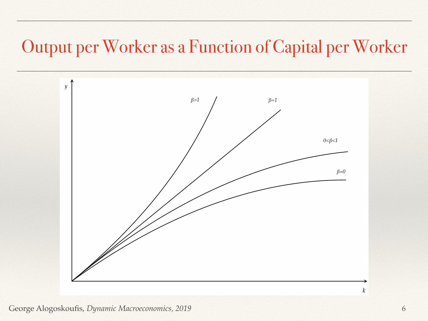
Output per Worker as a Function of Capital per Worker

6

k

β=0

0<β<1

β=1β>1

y


Externalities from the Accumulation of Capital and the Aggregate Production Function

For β=0, there is no effect of the aggregate accumulation of capital on labor efficiency, and we are back to an aggregate Cobb Douglas production function without externalities. The efficiency of labor depends only on the exogenous rate of technical progress g.

For 0<β<1 the accumulation of capital implies a positive externality on the efficiency of labor, but the aggregate marginal product of capital tends to fall as the economy accumulates more capital per worker. Capital accumulation leads to diminishing returns, although the productivity of capital declines at a slower rate than if there were no externalities.

For β=1, the aggregate marginal product of capital is constant, equal to total factor productivity A, and is not affected by the accumulation of capital. There are no diminishing returns to capital accumulation as the aggregate marginal product of capital is constant.

Finally, for β>1, the marginal product of capital increases with capital accumulation, but this assumption violates the condition of constant returns to scale for the aggregate economy.

7


A Learning by Doing Model of Endogenous Growth

8

We shall concentrate on the special case β=1, which implies endogenous growth without violating the assumption of constant returns to scale.

In the special case , aggregate output and output per worker take the form,

Aggregate output per worker is a linear function of capital per worker, although this is not the case for individual firms. The marginal and average productivity of capital is constant. Because of the linearity of the aggregate production function, the rate of growth of output per worker, or per capita income is equal to the rate of growth of capital per worker. The accumulation of capital per worker does not lead to diminishing returns. It thus follows that,

where is now endogenous, and is determined by the rate of accumulation of capital.

The rate of growth of aggregate output , is determined by the share of net investment to total output,

where denotes gross investment in physical capital and the depreciation rate.

β = 1

Y(t) = AK(t)

y(t) = A k(t)

g

· y(t)y(t)

=· k(t)k(t)

= g

g

g + n

g + n = ·Y(t)/Y(t) = ·K(t)/K(t) = (I(t)/K(t)) − δ = A(I(t)/Y(t)) − δ

I δ


AK Models of Endogenous GrowthThis endogenous growth model belongs to a class of models known as Models, from the form of the aggregate production function. The model with learning by doing was analyzed by Romer (1986), and we shall refer to it as the Arrow-Romer model.

An alternative model which is widely used is due to Rebelo (1991), who demonstrates that as long as there is a “core” of capital goods whose production does not involve non-reproducible factors, endogenous growth is compatible with production technologies that exhibit constant returns to scale. The simplest Rebelo (1991) model is a two sector model in which consumption goods are produced using both capital and labor, but capital goods are produced using only capital. In this class of models there are no externalities through “knowledge spillovers”, but in competitive equilibrium aggregate output turns out to be proportional to the capital stock. Because the Rebelo model is not based on externalities its policy implications are different than the policy implications of the Arrow-Romer model.

AKAK

AK

9


Determination of the Real Interest Rate and Real Wages

10

Firms operate under perfect competition and they maximize profits by taking the prices of inputs as given. Profit maximization implies that the real interest rate will be equal to the marginal product of capital for individual firms, and the real wage to the marginal product of labor for individual firms. These are given by,

The marginal productivity condition for the real interest rate implies that all firms will select the same capital per worker, as they face the same real interest rate and the same labor efficiency per worker. Therefore, .

Under the assumption that we have that ,

As a result, the real interest rate will be equal to,

The real interest rate is constant and equal to the private marginal product of capital, as calculated by each individual firm. Because of its small size, each competitive firm does not internalize the effects of its own choice of capital per worker on the aggregate capital stock per worker in the economy, treating labor efficiency as exogenously given. Labor efficiency depends on the aggregate capital stock per worker and not on the firm specific capital per worker. Because of this externality each firm underestimates the social marginal product of capital, and the real interest rate, as determined in competitive markets, is lower than the social (aggregate) marginal product of capital.

The real wage per worker is given by,

The real wage is a constant share of output per worker. If output per worker is growing at a rate , then the real wage per worker will also be growing at a rate . These properties are in accordance with Kaldor’s stylised facts.

r(t) = αA ki(t)α−1h(t)1−α − δ

w(t) = (1 − α)A ki(t)αh(t)1−α

ki(t) = k(t), ∀i

β = 1 h(t) = k(t)

r(t) = αA − δ

w(t) = (1 − α)A k(t) = (1 − α) y(t)

gg


Endogenous Growth and the Savings Rate in the Learning by Doing Model

11

Let us first assume that, as in the Solow model, consumer behavior is described by a constant savings rate. Per capita consumption is thus given by,

where is the exogenous savings rate.

Per capita output is given by,

In equilibrium, total output will be equal to consumption plus gross investment. In per capita terms,

Substituting the consumption function and the production function in the equilibrium condition, it follows that,

Dividing both sides we get that,

This determines the endogenous growth rate . The higher the exogenous savings (and investment) rate , and total factor productivity , the higher the growth rate of per capita income. On the other hand, population growth and the depreciation rate have a negative impact on the endogenous growth rate.

c(t) = (1 − s) y(t)

s

y(t) = A k(t)

y(t) = c(t) +· k(t) + (n + δ) k(t)

· k(t) = (sA − n − δ) k(t)k(t)

g =· k(t)k(t)

= sA − (n + δ)

g sA


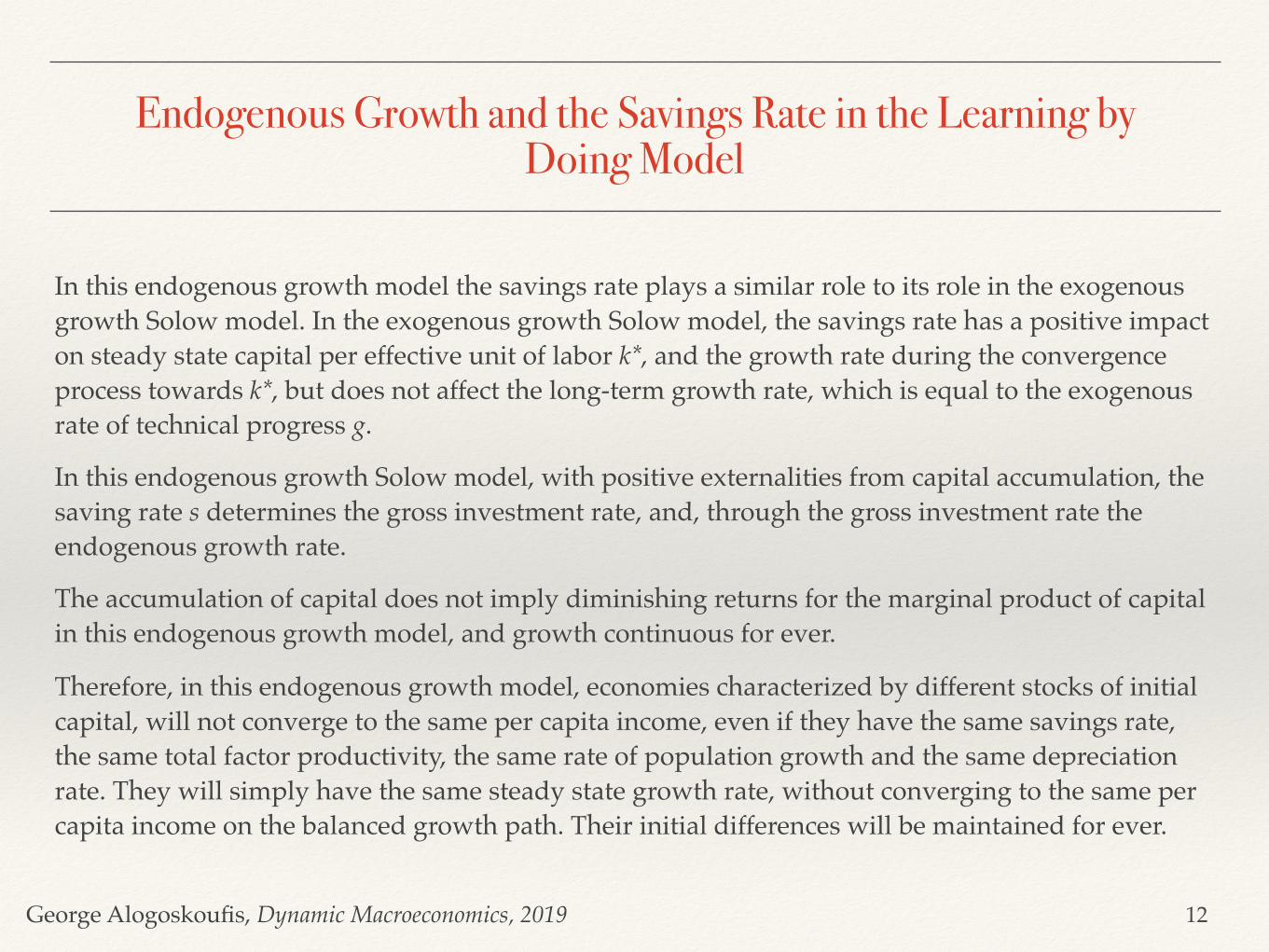
In this endogenous growth model the savings rate plays a similar role to its role in the exogenous growth Solow model. In the exogenous growth Solow model, the savings rate has a positive impact on steady state capital per effective unit of labor k*, and the growth rate during the convergence process towards k*, but does not affect the long-term growth rate, which is equal to the exogenous rate of technical progress g.

In this endogenous growth Solow model, with positive externalities from capital accumulation, the saving rate s determines the gross investment rate, and, through the gross investment rate the endogenous growth rate.

The accumulation of capital does not imply diminishing returns for the marginal product of capital in this endogenous growth model, and growth continuous for ever.

Therefore, in this endogenous growth model, economies characterized by different stocks of initial capital, will not converge to the same per capita income, even if they have the same savings rate, the same total factor productivity, the same rate of population growth and the same depreciation rate. They will simply have the same steady state growth rate, without converging to the same per capita income on the balanced growth path. Their initial differences will be maintained for ever.

12

Endogenous Growth and the Savings Rate in the Learning by Doing Model


Endogenous Growth in a Representative Household Learning by Doing Model

13

From the Euler equation for consumption, which describes the optimal savings behavior of the representative household, the rate of change of per capita consumption is given by,

Given that in this learning-by-doing endogenous growth model the real interest rate is constant and equal to ,, the rate of growth of per capita consumption is also constant, and given by,

This determines the endogenous growth rate , as on a balanced growth path all per capita variables grow at the same rate. If that was not so, either consumption or investment would eventually grow to be equal to output.

A higher pure rate of time preference of households, relative to the private marginal product of capital to firms (the real interest rate), results in a lower endogenous growth rate of per capita income and consumption. This is because a higher pure rate of time preference of households implies lower savings and a lower rate of accumulation of capital. On the other hand, a higher total factor productivity , or a higher private elasticity of firm output to capital , lead to a higher endogenous growth rate, as both result in a higher equilibrium real interest rate and higher savings and capital accumulation rates. For the opposite reason, the depreciation rate has a negative impact on the endogenous growth rate.

It is straightforward to show that in this model the savings rate is constant and determined by,

· c(t)c(t)

=1θ (r(t) − ρ)

αA − δ

· c(t)c(t)

=1θ (αA − δ − ρ) = g

g

A α

δ

s = 1 − ( c(t)y(t) ) =

n + g + δA

=1

θA (αA − (1 − θ)δ − ρ + θn)


The Determinants of Endogenous Growth in the Representative Household Learning by Doing Model

A higher pure rate of time preference of households ρ, relative to the private marginal product of capital to firms (the real interest rate), results in a lower endogenous growth rate of per capita income and consumption. This is because a higher pure rate of time preference of households implies lower savings and a lower rate of accumulation of capital.

On the other hand, a higher total factor productivity A, or a higher private contribution of capital to output α, lead to a higher endogenous growth rate, as both result in a higher equilibrium real interest rate, and higher savings and capital accumulation rates.

For the opposite reason, the depreciation rate δ has a negative impact on the endogenous growth rate.

A higher elasticity of inter-temporal substitution of consumption 1/θ results in a higher growth rate, as it facilitates savings.

14


The Inefficiency of Competitive Equilibrium in the Endogenous Growth Ramsey Model

15

Let us assume there is a social planner who maximizes the inter temporal utility function of the representative household, under the aggregate and not the private capital accumulation constraint. The first order condition for an optimum would we given by,

From the above inequality we can deduce that the endogenous growth rate in the competitive economy is lower than the socially efficient growth rate. This is because the competitive real interest rate ( ) underestimates the social net marginal product of capital ( ), which, because of the positive externality from capital accumulation, is higher than the private net marginal product of capital. Since the positive externality from capital accumulation is not reflected in the real interest rate, households have a smaller incentive to save and accumulate capital, and, as a result, the savings rate, the investment rate and the growth rate of the economy are lower than what would be socially optimal.

Thus, the competitive equilibrium is sub-optimal, and could be improved upon by a social planner who would choose savings and capital accumulation taking the externality into account. Various other policies, such as the subsidization of capital could improve efficiency in this case.

· c(t)c(t)

=1θ (A − δ − ρ) = g * >

1θ (αA − δ − ρ) = g

αA − δA − δ


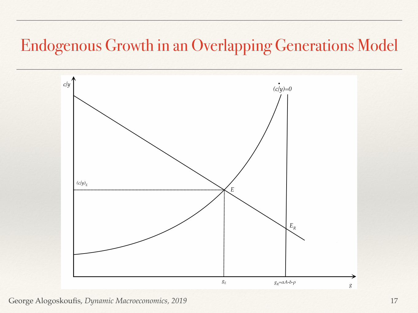
Endogenous Growth in an Overlapping Generations Model: The Behavior of Consumers

16

The change in per capita consumption in the Blanchard-Weil overlapping generations model is given by,

Dividing by per capita income , and after we replace the real interest rate from the marginal productivity condition and the capital output ratio from the aggregate production function , we get the following equation for the evolution of the ratio of private consumption to total output,

where, for any variable , we define its ratio to total output as .

From the per capita capital accumulation equation we get,

This suggests that the aggregate endogenous growth rate is equal to the net savings (=investment) rate, times total factor productivity, minus the depreciation rate. Because of constant returns to capital accumulation total factor productivity is equal to the (constant) average and marginal product of capital.

The last two equations can be used to determine the endogenous growth rate and the endogenous savings rate, .

,

The endogenous growth rate in an “Arrow-Romer-Blanchard-Weil” model is lower than in the corresponding “Arrow-Romer-Ramsey” model. The reason is that savings, and therefore capital accumulation and growth, are lower in the former model, due to the fact that current generations do not internalize the welfare of future generations.

· c(t) = [r(t) − ρ] c(t) − nρ k(t)

y(t) r(t) = aA − δY(t) = AK(t)

·c(t) = (r(t) − ρ − g)c(t) − nρk(t) = (αA − δ − ρ − g)c(t) − nρA−1

X Y x = X /Y

g = (1 − c(t)) A − n − δ

g + n

1 − c(t)

c(t) =nρA−1

αA − δ − ρ − gg = aA − δ − ρ −

nρ(1 − n − δ)A


Endogenous Growth in an Overlapping Generations Model

17

g

(c/y)=0

(c/y)E

gE

E

ER

gR=αA-δ-ρ

c/y


Endogenous and Exogenous Growth and Real Convergence

In endogenous growth models of the learning by doing model, there is no convergence process.

In exogenous growth models, any two economies characterized by the same parameters describing the technology of production, household preferences and economic policy, will converge to the same balanced growth path, even if they start from different initial conditions.

In endogenous growth models they will have the same endogenous growth rate, but they will not converge to the same per capita income. Their initial differences will remain for ever.

The available empirical evidence from post war international experience indicates that convergence cannot be dismissed easily.

18


Inter-temporal Path of Per Capita Income and Real Convergence in Endogenous and Exogenous Growth Models

19


Models of Human Capital Accumulation and Economic Growth

In the learning-by-doing endogenous growth model, endogenous growth is essentially a by-product of the accumulation of physical capital, because of the assumption that labor efficiency is a function of the aggregate physical capital stock per worker.

An alternative class of growth models (Lucas (1988), Mankiw, Romer and Weil (1992), Jones (2002)) emphasizes the education and training of workers and the accumulation of human capital that it implies. The accumulation of human capital brings about an increase in the efficiency of labor.

Under some conditions, this class of models can also lead to endogenous growth.

Endogenous growth in such models is not a by-product of physical capital accumulation, as in the Arrow-Romer model, but also depends on the factors that determine the accumulation of human capital.

20


The Production Function in Models with Human Capital Accumulation

21

Firms are competitive, and their production technology is Cobb-Douglas, of the form,

where, , and denotes the efficiency of labor at instant .

We shall assume that the efficiency of labor is a function of human capital per worker , and exogenous technical progress. This function takes the form,

where is human capital per worker, resulting from accumulated education and training, and a parameter which measures the relative contribution of human capital in the efficiency of labor. A fraction

of the efficiency of labor depends on technical progress, which grows at an exogenous rate .

Substituting for the efficiency of labor in the production function, we get,

where is aggregate human capital.

Y(t) = AK(t)α(h(t)L(t))1−α

0 < α < 1 h(t) t

h

h(t) = (h(t))γ(egt)1−γ

h 0 ≤ γ ≤ 1

1 − γ g

Y(t) = AK(t)αH(t)γ(1−α)(egtL(t))(1−γ)(1−α)

H(t) = h(t)L(t)


The Extended Solow Model (Mankiw, Romer and Weil)

22

We assume, generalizing the Solow model, that total household income is either consumed or invested in physical capital or invested in human capital. The percentage of output and income invested in physical capital equals , and the percentage invested in human capital equals . These percentages are considered exogenous, in the same way that the savings rate is assumed exogenous in the Solow model. The consumption function thus takes the form,

Furthermore we assume that , the depreciation rate, is the same for both physical and human capital. With these assumptions, the accumulation equations for physical and human capital are given by,

The equilibrium condition in the goods and services market in this case is given by,

sK sH

C(t) = (1 − sK − sH)Y(t)

δ

·K(t) = sKY(t) − δK(t)·H(t) = sHY(t) − δH(t)

Y(t) = C(t) + ·K(t) + ·H(t) + δ (K(t) + H(t))


The Extended Solow Model in Exogenous Efficiency Units of Labor

23

In the case where , we can divide the aggregate variables by the number of workers times the exogenous labor efficiency , and express the model as,

where, , , , .

These variables are defined as output, physical capital and human capital, per exogenous efficiency unit of labor.

0 < γ < 1L egt

y(t) = Ak(t)αh(t)γ(1−α)

·k(t) = sK y(t) − (n + g + δ)k(t)·h(t) = sHy(t) − (n + g + δ)h(t)

c(t) = (1 − sK − sH)y(t)

y(t) = Y(t)egtL(t) c(t) = C(t)

egtL(t) k(t) = K(t)egtL(t) h(t) = H(t)

egtL(t)


The Balanced Growth Path in the Extended Solow Model of Exogenous Growth (Mankiw, Romer and Weil)

24

On the balanced growth path, all per capita variables grow at the rate of exogenous technical progress . It therefore follows that,

It thus follows that,

on the balanced growth path, the ratio of physical to human capital is constant, and equal to the ratio of the investment rates in physical and human capital respectively. This follows because equilibrium investment on the balanced growth path is a proportion of both physical and human capital, per exogenous efficiency unit of labor.

Substituting in the production function and solving, it follows that,

, ,

Hence, per capita output on the balanced growth path is given by,

g

sK y* = sK A(k*)α

(h*)γ(1−a)

= (n + g + δ)k*

sH y* = sH A(k*)α

(h*)γ(1−a)

= (n + g + δ)h*

k* =sK

sHh*

n + g + δ

h* = (A (sKαsH1−α)

n + g + δ )1

(1 − γ)(1 − α)

k* = (A (sK

1−γ(1−α)sHγ(1−α))

n + g + δ )1

(1 − γ)(1 − α)

y* =A (sKαsH

γ(1−α))(n + g + δ)α+γ(1−α)

1(1 − γ)(1 − α)

y*(t)

y*(t) = y*egt =A (sKαsH

γ(1−α))(n + g + δ)α+γ(1−α)

1(1 − γ)(1 − α)

egt


The Balanced Growth Path in the Extended Solow Model of Exogenous Growth

The level of per capita output on the balanced growth path depends positively on total factor productivity A and the shares of output invested in physical and human capital (sK και sH).

As in the original Solow model it depends negatively on the population growth rate n, the rate of exogenous technical progress g, and the depreciation rate δ.

The rate of growth of per capita output on the balanced growth path is equal to the rate of exogenous technical progress g.

Thus, in the case where we have an extended Solow model of exogenous growth. In this model, human capital accumulation plays a role similar to physical capital accumulation in the original Solow model. As the accumulation of human capital causes an increase in the marginal productivity of physical capital and vice versa, the convergence process continues for longer, but eventually the economy converges to a balanced growth path where growth in per capita income is equal to the exogenous rate of technical progress.

y*(t) = y*egt =A (sKαsH

γ(1−α))(n + g + δ)α+γ(1−α)

1(1 − γ)(1 − α)

egt

0 < γ < 1

25


Endogenous Growth in the Extended Solow Model (Mankiw, Romer and Weil)

26

If , there is no exogenous technical progress. The efficiency of labor only depends on accumulated human capital. The model is this case is an endogenous growth model. Setting in the aggregate production function we get,

, where, , , .

In this model, the balanced growth path would be defined by,

,

On the balanced growth path, the ratio of physical to human capital is stabilized at the ratio of the investment rates in physical and human capital. Because both physical and human capital are growing at the same rate, we have endogenous growth. The accumulation of physical capital causes an increase in income, that in turn causes an increase in human capital through expenditure on education and training. This in turn leads to a further rise in output, which causes new investment in physical capital. The parallel accumulation of physical and human capital leads to endogenous growth.

The endogenous growth rate depends positively on total factor productivity , and a weighted average of the income ratios invested in physical and human capital and . The rate of growth of population , and the depreciation rate , have a negative impact on the endogenous growth rate.

In all other respects, the properties of the endogenous growth, extended Solow model, are similar to those of the learning by doing model of Arrow and Romer. The main difference is that in this extended Solow model, the accumulation of human capital is not a simple by-product of physical capital accumulation, but the result of explicit investment on human capital, through spending on education and training.

γ = 1γ = 1

y(t) = A k(t)αh(t)1−α y = Y/L k = K /L h = H /L

k*(t)h*(t)

=sK

sHg =

· y*(t)y*(t)

= AsαKs1−α

H − (n + δ)

AsK sH n δ


The Jones Model of Human Capital Accumulation

27

An alternative model, is one in which human capital depends on the time span devoted to education and training. We assume that workers spend part of their time in education and training, and that this investment of time involves a rate of return . The model is analyzed in Jones(2002).

The production technology is described by the production function,

The efficiency of labor per employee is determined by .

The function determines human capital per worker, as a function of the time span devoted to education and training, and the rate of return of investment in human capital . A plausible form of this function is the exponential function. The exponential form is plausible because it implies that the proportional change in the function with respect to the time devoted to education and training is equal to the rate of return . We shall therefore assume that,

In this model, output per worker (per capita output) is given by,

Combining this with the savings assumption of the Solow model, i.e., that there is an exogenous constant savings rate, per capita output on the balanced growth path is determined by,

Per capita output on the balanced growth path is a positive function of the amount of time spent in education and training , and the rate of return on investment in human capital . However, in all other respects, this model is an exogenous growth model, similar to the Solow model.

v ψ

Y(t) = AK(t)α(h(t)L(t))1−α

h(t) = h(v, ψ)egt

h(v, ψ) vψ

ψ

h(v, ψ) = eψ v

y(t) = A k(t)α(eψ vegt)1−α

y*(t) = A( sAn + g + δ )

α1 − α

eψ vegt

vψ


The Lucas Endogenous Growth ModelAn alternative model of investment in human capital is the endogenous growth model of Lucas (1988), which is based, in part, on Uzawa (1965).

Lucas assumed that labor efficiency is equal to human capital per worker, .

With regard to the production of human capital per worker he assumes that this depends on the existing stock of human capital per worker, times the proportion of non-leisure time that workers devote to education and training. He thus assumes that,

Only human capital is required for the production of human capital. is defined as the proportion of the non-leisure time of households that is devoted to the production of goods and services, while is the proportion of time devoted to education and training. Education and training results in the accumulation of human capital. is the productivity of human capital in the production of new human capital, is the population growth rate and the depreciation rate of human capital, assumed for simplicity to be equal to that of physical capital.

On the balanced growth path, will be constant at . Taking the integral of the human capital accumulation equation, we get,

Lucas assumed that is chosen optimally by a representative household in order to maximize its intertemporal utility of consumption. As a result, the choice of depends both on the preferences of the representative household, and on the technological parameters characterizing the production of goods and services and human capital. From the form of the human capital equation, it follows that the endogenous growth rate is equal to , which works like the exogenous rate of technical progress in exogenous growth models. The higher is the steady state proportion of non-leisure time devoted to education and training, the higher the endogenous growth rate. In the Lucas model, is chosen endogenously, and, in conjunction with the exogenous , and , determines the steady state growth rate of per capita output.

h(t) = h(t)

·h(t) = ζ(1 − u(t))h(t) − (n + δ)h(t)

u1 − u

ζ nδ

u u*

h(t) = e(ζ(1−u*)−(n+δ))t

uu

g = ζ(1 − u*) − (n + δ)

1 − u* ζ δ n

28


Models of the Production of Ideas and Innovations

A final category of growth models, model technical progress as the result of ideas and innovations, that lead to higher total factor productivity or labor efficiency.

These models emphasize the externalities involved in generating new ideas and innovations that increase the efficiency of production. As the learning by doing model of Arrow emphasizes the externalities from capital accumulation, so the ideas and innovations models emphasize the externalities of the production of ideas and innovations.

Although models in this category, sometimes called research and development (R&D) models, date from the late 1960s, the microeconomic foundations of these models and their implications for the functioning of markets were developed in the early 1990s, inspired by the work of Romer (1990). These models, under certain conditions, can lead to endogenous growth as well.

29


Key Features of Ideas and InnovationsA crucial assumption of such models is that ideas and innovations can improve the efficiency of production, either through total factor productivity or through labor efficiency.

These models recognize that, unlike most other goods and services, the use of an idea and/or innovation by a particular firm, or employee, does not prevent to use of the same idea and innovation from other firms or workers. The use of a particular idea or innovation is non rivalrous, in contrast to the use of a particular machine or a specific employee. From the time an idea or innovation has been produced, anyone with knowledge of this idea can use it, independently of how many others use it simultaneously. If a firm uses a specific machine or a particular employee, it automatically excludes any other firm from simultaneously using this same machine or this same employee. The property of non-rivalry gives ideas and innovations a character of a quasi public good.

On the other hand, in contrast to purely public goods, the use of an idea can be partially excludable by law. This allows the producer of an idea to charge for the use of his idea. For example, if an idea or innovation is legally covered by a patent, then a firm or an employee who wants to use this idea or innovation will have to pay a fee to the holder of the patent, for their copyright.

30


Externalities and the Production of Ideas and Innovations

Purely public goods and services are both non rivalrous and non excludable. Other goods and services, such as ideas that can be covered by copyright laws, may be non rivalrous, but may be excludable. Consequently, the producers of goods and services that use an idea or innovation, may be charged for the benefits arising from their use.

The production of non rivalrous and non excludable goods and services implies externalities, which are not reflected in the remuneration of producers of these goods and services. Goods and services that result in positive externalities, such as ideas and innovations, will be produced in smaller quantities than would be socially desirable, and goods and services that result in negative externalities, such as pollution of the environment, will be produced in larger quantities than would be socially desirable.

If the use of ideas and innovations is both non rivalrous and non excludable, then the market will produce fewer ideas and innovations than would be socially desirable. However, if the use of ideas and innovations can be made excludable by the protection of the law on copyright or a patent, then the production of ideas and innovations can rise, as producers of ideas and innovations will be paid for the value of their product.

31


The Key Elements of an Ideas and Innovations Growth Model

In order to present the key elements of a growth model based on the production of ideas and innovations we start with the production function of goods and services. We assume a Cobb-Douglas production function, of the form,

where is the existing aggregate stock of ideas and innovations, affecting the efficiency of labor in the goods and services sector, and is the number of workers who are employed in the goods and services sector.

Apart from goods and services, the economy produces new ideas and innovations. The new ideas and innovations produced per instant are proportional to the number of research workers, i.e., those employed in the production of ideas and innovations. This relationship can be written as,

where is the number of workers employed in the production of ideas and innovations, which we shall call research workers or researchers. is the average productivity of research workers.

We assume that the average productivity of research workers is a positive function of the total stock of ideas and innovations and a negative function of the number of research workers. The existing stock of ideas and innovations makes every researcher more productive. However, we shall assume that this effect is subject to diminishing returns. On the other hand, as the number of researchers increases, the probability of duplication of effort, that is the probability of simultaneous production of the same idea or innovation by more than one researcher, increases. Thus, the average productivity of research workers falls with the number of researchers. In particular, we will assume that the productivity function of research workers, with the characteristics highlighted above, takes the form,

where, , , .

Y(t) = AK(t)α(H(t)Ly(t))1−α

H Ly

·H(t) = h(H(t), Lh(t))Lh(t)

Lhh( . )

h(H(t), Lh(t)) = hH(t)βLh(t)γ−1

h > 0 0 < β < 1 0 < γ < 1

32


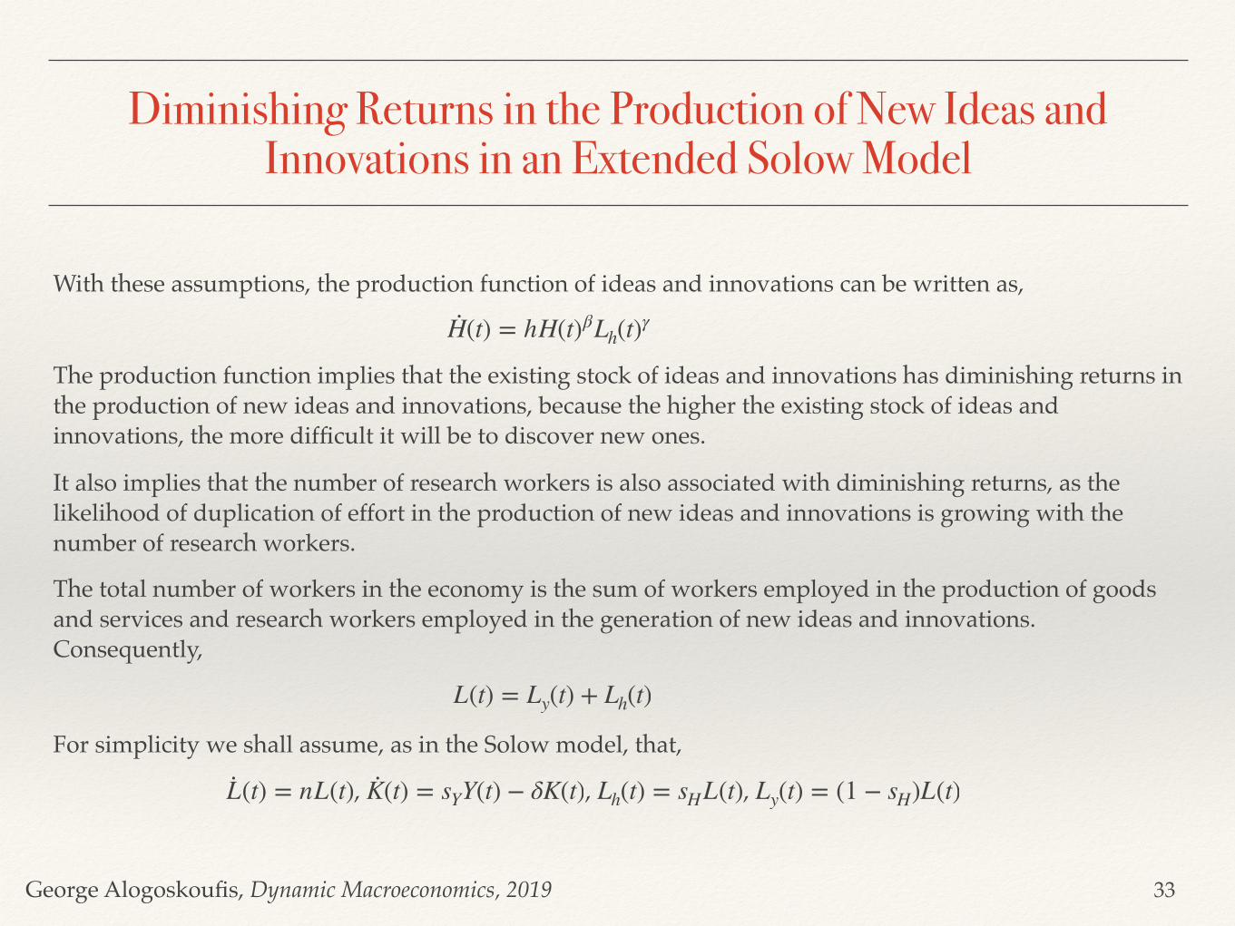
Diminishing Returns in the Production of New Ideas and Innovations in an Extended Solow Model

With these assumptions, the production function of ideas and innovations can be written as,

The production function implies that the existing stock of ideas and innovations has diminishing returns in the production of new ideas and innovations, because the higher the existing stock of ideas and innovations, the more difficult it will be to discover new ones.

It also implies that the number of research workers is also associated with diminishing returns, as the likelihood of duplication of effort in the production of new ideas and innovations is growing with the number of research workers.

The total number of workers in the economy is the sum of workers employed in the production of goods and services and research workers employed in the generation of new ideas and innovations. Consequently,

For simplicity we shall assume, as in the Solow model, that,

, , ,

·H(t) = hH(t)βLh(t)γ

L(t) = Ly(t) + Lh(t)

·L(t) = nL(t) ·K(t) = sYY(t) − δK(t) Lh(t) = sHL(t) Ly(t) = (1 − sH)L(t)

33


The Determination of the Rate of Technical Progress

34

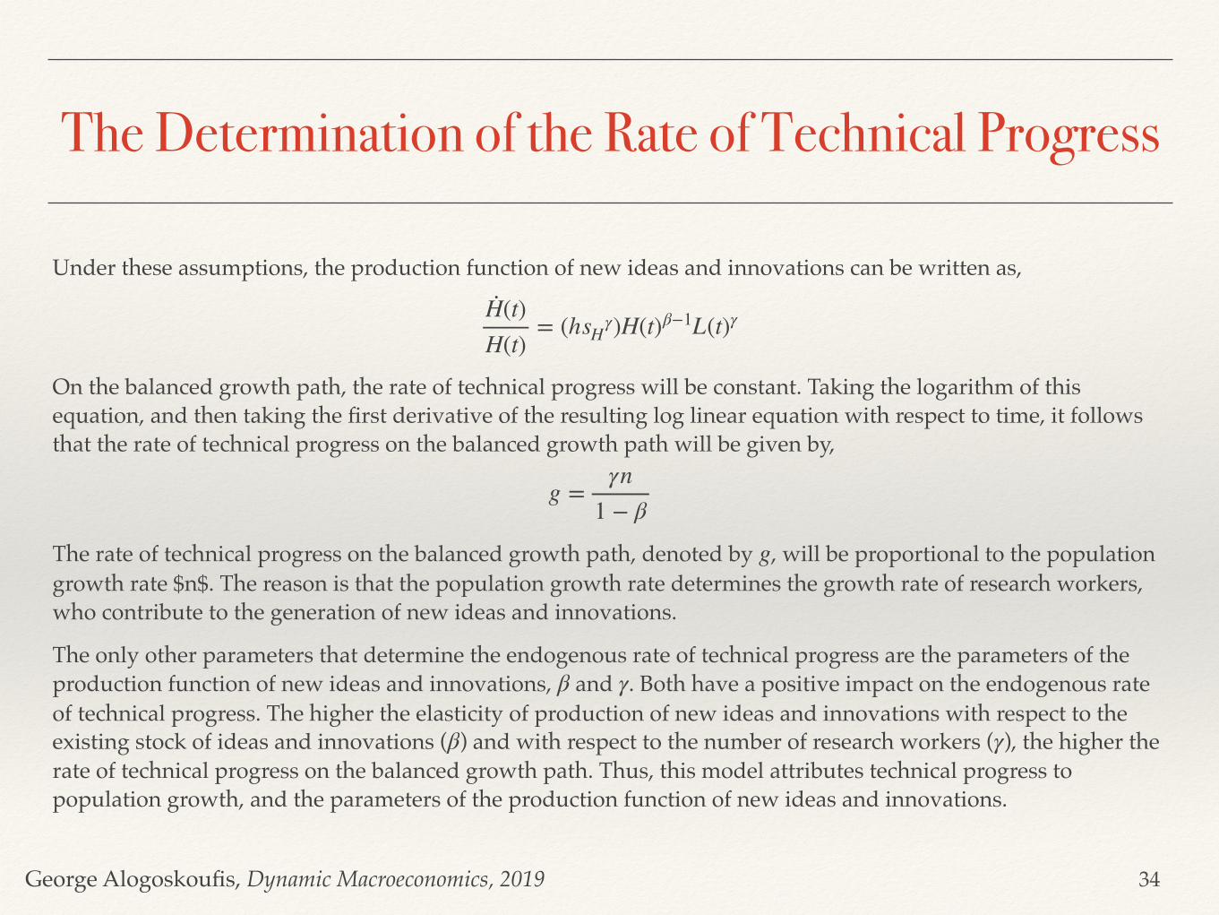
Under these assumptions, the production function of new ideas and innovations can be written as,

On the balanced growth path, the rate of technical progress will be constant. Taking the logarithm of this equation, and then taking the first derivative of the resulting log linear equation with respect to time, it follows that the rate of technical progress on the balanced growth path will be given by,

The rate of technical progress on the balanced growth path, denoted by , will be proportional to the population growth rate $n$. The reason is that the population growth rate determines the growth rate of research workers, who contribute to the generation of new ideas and innovations.

The only other parameters that determine the endogenous rate of technical progress are the parameters of the production function of new ideas and innovations, and . Both have a positive impact on the endogenous rate of technical progress. The higher the elasticity of production of new ideas and innovations with respect to the existing stock of ideas and innovations ( ) and with respect to the number of research workers ( ), the higher the rate of technical progress on the balanced growth path. Thus, this model attributes technical progress to population growth, and the parameters of the production function of new ideas and innovations.

·H(t)H(t)

= (hsHγ)H(t)β−1L(t)γ

g =γn

1 − β

g

β γ

β γ


The Balanced Growth Path in the Ideas and Innovations Solow Model

35

On the balanced growth path, all per capita variables grow at the endogenous rate of technical progress . Variables per efficiency unit of labor are determined in a way similar to the corresponding Solow model. One can show that, on the balanced growth path, we shall have,

where, , , , and superscript * denotes the value of the corresponding variable on the balanced growth path.

On the balanced growth path the model behaves exactly as the Solow model, except for the fact that the rate of technical progress is determined endogenously, and depends on population growth and the parameters that characterize the production function of new ideas and innovations.

g

k* = ( sY A(1 − sH)1−α

n + g + δ )1

1 − α

y* = A(1 − sH)1−α(k*)α

c* = (1 − sY)y*

H*(t) = ( (1 − β)hγn )

11 − β

(sHL(0))γ

1 − βe( γn1 − β )t

k = K /HL y = Y/HL c = C/HL

g


Conclusions from the Generalized Growth Models

We have analyzed more general growth models, which, instead of relying only on the assumption of exogenous technical progress, are based on the assumptions of either external effects from the accumulation of physical capital, or investment in human capital, or even the endogenous generation of ideas and innovations.

Endogenous growth models do not necessarily provide for convergence, as the corresponding exogenous growth models. However, the available empirical evidence from post war international experience (see for example Mankiw, Romer and Weil (1992) and Barro (1997)) indicates that the issue of convergence of per capita incomes of the various economies cannot be dismissed easily. This convergence can be explained by generalized models in which there is learning by doing, accumulation of human capital and endogenous technical progress, but not to a degree that would completely neutralize the diminishing returns from the accumulation of physical capital.

Consequently, generalized exogenous growth models, in which there are externalities from capital accumulation, and/or accumulation of human capital and endogenous technical progress, could, in principle, explain most of the aspects of the process of economic growth that cannot be explained by the original Solow model, or the corresponding representative household or overlapping generations models.

36


Unified Growth Theory and the Transition from Stagnation to Growth

The models we have analyzed in this and the preceding chapters aim to explain the process of economic growth since the take off in economic growth following the industrial revolution. They have little if anything to say about the long centuries of economic stagnation that preceded this period, as we have already documented. They have also very little to say concerning the reasons behind the transition from stagnation to economic growth, and also very little to say about why some countries have been successful in creating the conditions for sustained growth and others have not.

A recent development in the theory of economic growth is the so called unified growth theory. Unified growth theory aims to explain both the process of economic growth after 1820, and the centuries of economic stagnation that preceded it.

Unified growth theory first concentrates on the conditions that prevailed in the so called ‘Malthusian era’, when technological innovations or new resources such as land resulted in an increase in population rather than an increase in per capita income and living standards. Thus, unified growth theory treats population growth as endogenous.

Second, it attempts to explain the transition from stagnation to growth, following the industrial revolution, as a period which, because of the high rate of technological innovation and other social developments, resulted in a demographic transition from high to low population growth rates, allowing for a sustained rise in living standards.

This process was facilitated by social changes which gave emphasis to education and training and the accumulation of human capital.

Unified growth theory combines historical and empirical research with theoretical growth models to explain both the Malthusian process of economic fluctuations that led to fluctuations in population growth rates but more or less stagnant living standards, and the post-Malthusian take off in living standards in the industrial economies.

Unified growth theory does not necessarily clash with or refute the models of economic growth that we have examined. However, it treats them a partial and incomplete accounts of the process of economic growth, and as accounts that are mainly relevant for the post-Malthusian era in the industrial economies. It gives emphasis to the interaction between technical progress and population growth, which are treated as endogenous variables and not exogenous parameters, as in most of the models that we have examined.

37


Institutions and long-run growthThe models we have presented in this book explain long-run economic growth as a result of the accumulation of physical and human capital and technological change. Why then don't all countries adopt policies that are friendly to such processes. This way, the large differences in per capita income between the developed and less developed world would gradually disappear.

One of the reasons that has been put forward, along with geography and cultural differences, is the role of institutions. The role of institutions has been emphasized by economic historians for a long time, as they have treated the accumulation of physical and human capital and technological progress as only the proximate and not the fundamental determinants of long-run economic growth. As North and Thomas (1973), put it: ``the factors we have listed (innovation, economies of scale, education, capital accumulation, etc.) are not causes of growth; they are growth'' (p. 2, italics in original). Factor accumulation and innovation are only proximate causes of growth. In North and Thomas's view, and in the view of many other economic historians, the fundamental explanation of comparative growth is differences in institutions. Of primary importance to economic outcomes are economic and political institutions such as civil and property rights, the existence and the imperfections of markets, the nature of the political system etc.

Economic and political institutions are important because they influence the structure of economic incentives. Without the protection of property rights, individuals will not have the incentive to invest in physical or human capital or to adopt more efficient technologies. Economic institutions are also important because they help to allocate resources to their most efficient uses, they determine who gets profits, revenues and residual rights of control. When markets are missing or ignored, potential gains from trade go unexploited and resources are misallocated. Societies with economic institutions that facilitate and encourage factor accumulation, innovation and the efficient allocation of resources will prosper.

38


The Economic Analysis of Institutions and Long-Run growth

Economists also turned their attention to the role of institutions, as exemplified by the pioneering empirical study of Acemoglou et al (2001) and the literature that is sparked. In recent years, a number of authors have formalized these ideas investigating the effects of institutions on the process of long-run growth. The basic premises of this approach are as follows:

First, economic institutions matter for economic growth because they shape the incentives to invest in physical and human capital and technology, and improve the organization of production. Although cultural and geographical factors may also matter for economic performance, differences in economic institutions are the major source of cross-country differences in economic growth and prosperity. Economic institutions not only determine the aggregate economic growth potential of the economy, but also an array of economic outcomes, including the distribution of resources in the present and the future.

Second, economic institutions are treated as endogenous. They are determined collectively, in large part for their economic consequences. Not all individuals and groups will prefer the same set of economic institutions because different economic institutions lead to different distributions of resources. Consequently, there will typically be conflicts of interest among various groups and individuals over the choice of economic institutions. These conflicts of interest are resolved through the political process.

Third, the distribution of political power in society is also treated as endogenous. Political institutions, similarly to economic institutions, determine the constraints on and the incentives of the key actors in the political sphere. Political power can be either de jure (institutional) or de facto. The de facto power of particular groups depends on their economic resources, which determine both their ability to use (or misuse) existing political institutions and also their option to hire and use force against other groups.

39


The Persistence of InstitutionsThere are two sources of persistence in the behavior of such a system:

First, political institutions are durable, and typically, a sufficiently large change in the distribution of political power is necessary to cause a change in political institutions, such as, for example, a transition from dictatorship to democracy.

Second, when a particular group is rich relative to others, this will increase its de facto political power and enable it to push for economic and political institutions favorable to its interests. This will tend to reproduce the initial relative wealth disparity in the future.

Despite these tendencies for persistence, the framework also emphasizes the potential for change. In particular, ‘shocks’, including changes in technologies and the international environment can modify the balance of (de facto) political power in society and can lead to major changes in political institutions and therefore in long-run economic growth.

40


The New Stylized Facts of Economic Growth

In 1961, Nicholas Kaldor highlighted six ‘stylized' facts to summarize the patterns that economists had discovered in national income accounts and to check the growth models being developed to explain them. Jones and Romer (2010) attempted at redoing this exercise it order to investigate how much progress has been made. They came up with additional stylized facts that a satisfactory growth model should account for. Their list of additional stylized facts, is the following:

1. Increases in the extent of the market. Increased flows of goods, ideas, finance, and people, via globalization, as well as urbanization, have increased the extent of the market for all workers and consumers.

2. Accelerating growth. For thousands of years, growth in both population and per capita GDP has accelerated, rising from virtually zero to the relatively rapid rates observed in the last century.

3. Variation in growth rates. The variation in the rate of growth of per capita GDP increases with the distance from the technology frontier.

4. Large income and total factor productivity (TFP) differences. Differences in measured inputs explain less than half of the enormous cross-country differences in per capita GDP.

5. Increases in human capital per worker. Human capital per worker is rising dramatically throughout the world.

6. Long-run stability of relative wages. The rising quantity of human capital, relative to unskilled labor, has not been matched by a sustained decline in its relative price.

41


Accounting for the New Stylized Facts of Economic Growth

Whereas Kaldor's original facts were accounted for almost entirely using the neoclassical growth model, the facts highlighted by Jones and Romer reveal the broader reach of modern growth theory. To capture these facts, a growth model must consider the interaction between ideas, institutions, population, and human capital.

Two of the major facts of growth, its acceleration over the very long run and the extraordinary rise in the extent of the market associated with globalization, are readily understood as reflecting the defining characteristic of ideas, their non-rivalry.

The next two major facts, the enormous income and total factor productivity differences across countries, as well as the stunning variation in growth rates for countries far behind the technology frontier, testify to the importance of institutions and institutional change.

The final two facts of Jones and Romer parallel two of Kaldor's original observations, but while his emphasis was on physical capital, the emphasis in modern growth theory is on human capital. Human capital per worker is rising rapidly, and this occurs despite no systematic trend in the wage premium associated with education.

According to Jones and Romer, these facts also reveal important complementarities among the key endogenous variables.

The virtuous circle between population and ideas accounts for the acceleration of growth.

Institutions may have their most important effects on cross-country income differences by hindering the adoption and utilization of ideas from throughout the world. Institutions like public education and the university system are surely important for understanding the growth in human capital. And institutions are themselves based on ideas - inventions that shape the allocation of resources - and the search for better institutions is unending.

Finally, the rising extent of the market, which raises the return to ideas and to the human capital that is a fundamental input to the production of ideas, may help explain why the college wage premium has not fallen systematically, despite the huge increases in the ratio of college graduates to high school graduates.

42


Notes on the Literature

For comprehensive surveys of the extensive recent literature on economic growth and a number of additional models, including political economy models, see The Handbook of Economic Growth, edited by Aghion and Durlauf (2005) and Aghion and Durlauf (2014). There are also excellent presentations in books by Acemoglou (2009), Aghion and Howitt (2009), and Barro and Sala-i-Martin (2004). On unified growth theory see Galor (2011).

43

athens university of economics and business 9. externalities, … · 2019-11-27 · george...

Documents