ESSAY

The Heat Equation and theAtiyah-Singer Index Theorem

UNIVERSITY OF CAMBRIDGEMATHEMATICAL TRIPOS PART III

APRIL 29, 2015

written byDAVID REUTTER

Christ’s College

Contents

Introduction 3

1 Spin Geometry 8

1.1 Clifford Algebras . . . . . . . . . . . . . . . . . . . . . . . . . . . . . . . . . . . . . . . . . . . 8

1.1.1 Basic Definitions and Properties . . . . . . . . . . . . . . . . . . . . . . . . . . . . . . . 8

1.1.2 Grading, Filtration and the Symbol Map . . . . . . . . . . . . . . . . . . . . . . . . . . . 10

1.2 The Spin and Pin Groups . . . . . . . . . . . . . . . . . . . . . . . . . . . . . . . . . . . . . . . 12

1.2.1 Subgroups of Clpnq . . . . . . . . . . . . . . . . . . . . . . . . . . . . . . . . . . . . . . 12

1.2.2 The Groups Pinn and Spinn . . . . . . . . . . . . . . . . . . . . . . . . . . . . . . . . . 13

1.2.3 The Lie Algebra spinn . . . . . . . . . . . . . . . . . . . . . . . . . . . . . . . . . . . . 15

1.3 Spinor Representations . . . . . . . . . . . . . . . . . . . . . . . . . . . . . . . . . . . . . . . . 16

1.4 Fermions and Bosons . . . . . . . . . . . . . . . . . . . . . . . . . . . . . . . . . . . . . . . . . 19

1.5 Spin Geometry . . . . . . . . . . . . . . . . . . . . . . . . . . . . . . . . . . . . . . . . . . . . 21

1.5.1 Differential Geometry . . . . . . . . . . . . . . . . . . . . . . . . . . . . . . . . . . . . 21

1.5.2 Spin Manifolds . . . . . . . . . . . . . . . . . . . . . . . . . . . . . . . . . . . . . . . . 24

1.5.3 Spin Connection . . . . . . . . . . . . . . . . . . . . . . . . . . . . . . . . . . . . . . . 25

1.5.4 Formal Adjoints . . . . . . . . . . . . . . . . . . . . . . . . . . . . . . . . . . . . . . . 29

2 The Atiyah-Singer Index Theorem 32

2.1 Sobolev Spaces . . . . . . . . . . . . . . . . . . . . . . . . . . . . . . . . . . . . . . . . . . . . 32

2.1.1 Sobolev Theory for Dirac Operators . . . . . . . . . . . . . . . . . . . . . . . . . . . . . 34

2.2 Fredholm Operators and Index . . . . . . . . . . . . . . . . . . . . . . . . . . . . . . . . . . . . 37

2.3 The Proof of the Index Theorem . . . . . . . . . . . . . . . . . . . . . . . . . . . . . . . . . . . 39

2.3.1 Superspaces and Supertraces . . . . . . . . . . . . . . . . . . . . . . . . . . . . . . . . . 39

1

2.3.2 The McKean-Singer formula - Step One . . . . . . . . . . . . . . . . . . . . . . . . . . . 40

2.3.3 The Heat Equation - Step Two . . . . . . . . . . . . . . . . . . . . . . . . . . . . . . . . 41

2.3.4 The Asymptotic Expansion of the Heat Kernel - Step Three . . . . . . . . . . . . . . . . 44

2.3.5 Getzler Scaling - Step Four . . . . . . . . . . . . . . . . . . . . . . . . . . . . . . . . . . 45

2.4 The Index Theorem . . . . . . . . . . . . . . . . . . . . . . . . . . . . . . . . . . . . . . . . . . 51

3 Applications and Outlook 53

3.1 First Examples . . . . . . . . . . . . . . . . . . . . . . . . . . . . . . . . . . . . . . . . . . . . 53

3.2 The Riemann Roch Theorem . . . . . . . . . . . . . . . . . . . . . . . . . . . . . . . . . . . . . 54

3.3 The Index Theorem in Seiberg-Witten Theory . . . . . . . . . . . . . . . . . . . . . . . . . . . . 57

3.4 Outlook . . . . . . . . . . . . . . . . . . . . . . . . . . . . . . . . . . . . . . . . . . . . . . . . 59

Appendix 60

A The Asymptotic Expansion . . . . . . . . . . . . . . . . . . . . . . . . . . . . . . . . . . . . . . 60

B Mehler’s Formula . . . . . . . . . . . . . . . . . . . . . . . . . . . . . . . . . . . . . . . . . . . 64

2

Introduction

The Atiyah-Singer index theorem is a milestone of twentieth century mathematics. Roughly speaking, it relatesa global analytical datum of a manifold - the number of solutions of a certain linear PDE - to an integral of localtopological expressions over this manifold. The index theorem provided a link between analysis, geometry andtopology, paving the way for many further applications along these lines.

An operator T : H1 Ñ H2 between Hilbert spaces is called Fredholm if both its kernel and its cokernel are finitedimensional. The index of such an operator is defined to be the difference between these two quantities. Everyelliptic differential operator between vector bundles over a compact manifold defines a Fredholm operator andtherefore has a finite index. The index is a very well behaved analytical quantity which is, for example, stableunder compact perturbations. This prompted Israel Gelfand in 1960 to conjecture that the index of an ellipticoperator is a topological invariant and to ask for an explicit expression of this index in terms of other invariants.

The easiest example of such an ‘index theorem’ is the Toeplitz theorem.Let L2pS1q “ t

ř

nPZ anzn |

ř

nPZ |an|2 ă 8u and let H :“ t

ř8

n“0 anzn |

ř8

n“0 |an|2 ă 8u be the Hardy

space with projector Π : L2pS1q Ñ H. For f P CpS1q, the Toeplitz operator is the map Tf :“ Π Mf |H : HÑ H,where Mf : L2pS1q Ñ L2pS1q denotes the multiplication operator with f . Using basic properties of the indexone can show that Tf is Fredholm if and only if f is non-vanishing and

indpTf q “ ´ winding number of f around 0. (1)

If f is differentiable, we can use the logarithmic derivative and express this as indpTf q “ ´1

2πi

ş

S1f 1

f dz.

In guise of the ‘classical index theorems’ - the Signature theorem, the Chern-Gauss-Bonnet theorem and theHirzebruch-Riemann-Roch theorem - more complicated index theorems had already been known for specificelliptic operators.

In 1963, Michael Atiyah and Isadore Singer solved Gelfand’s problem and announced their theorem, expressingthe index of a general elliptic operator on a compact oriented manifold in terms of certain characteristic classes -subsequently dubbed ‘topological index’ - of this manifold.In the following essay, we explain how this can be done for a particular class of elliptic operators - twisted Diracoperators on even dimensional compact spin manifolds - and then indicate how this solves the general problem.We will now give a brief overview of our main results.

Spin Geometry

The Clifford algebra ClCpV q of a vector space V with inner product p¨, ¨q is the complex algebra generated byvectors v P V with relations

v1 ¨ v2 ` v2 ¨ v1 “ ´2pv1, v2q. (2)

As a vector space, the Clifford algebra is isomorphic to the (complex) exterior algebra ΛV . Using an orthonormalbasis e1, . . . , en of V , this isomorphism is given by

σ : ClCpV q Ñ ΛV ei1 ¨ ¨ ¨ eik ÞÑ ei1 ^ ¨ ¨ ¨ ^ eik . (3)

3

If M is a Riemannian manifold we define the Clifford algebra ClCpMqx at the point x to be the Clifford algebraof T˚xM with the induced Riemmanian metric. The Levi-Civita connection on TM extends to a connection on theexterior bundle ΛT˚M which induces a connection ∇ on the Clifford algebra bundle ClCpMq.

A hermitian vector bundle E “ E` ‘ E´ with compatible connection ∇E is said to be a Clifford bundle if there isan algebra bundle homomorphism c : ClCpMq Ñ EndpEq such that for a section α of T˚M and ε, ε1 P E

p1q cpαq swaps E` and E´, p2q`

cpαqε, ε1˘

``

ε, cpαqε1˘

“ 0, p3q r∇EX , cpαqs “ cp∇Xαq. (4)

The Dirac operatorD on a Clifford bundle E is the formally self-adjoint elliptic operator defined in terms of a localframe e1, . . . , en of TM (with corresponding dual frame e1, . . . , en) as

D :“

dimpMqÿ

i“1

cpeiq∇Eei . (5)

In this essay, we will focus on a specific example of a Clifford bundle - the twisted spinor bundle on an evendimensional spin manifold. A spin manifold is an oriented Riemannian manifold fulfilling certain topologicalconditions. On an even dimensional spin manifold, there exists a Clifford bundle S “ S

`‘ S

´ such thatc : ClCpMq Ñ EndpSq is an isomorphism. In fact, the fibrewise representation Sx of ClCpMqx is the uniqueirreducible representation of the Clifford algebra. The Dirac operator D on this so called spinor bundle is formallyself-adjoint and maps sections of S˘ to S¯. If V is a hermitian vector bundle with compatible connection, we candefine the twisted spinor bundle

E “ S ‘ V “´

S`b V

¯

‘

´

S´b V

¯

(6)

with corresponding Dirac operator DV .If M is even-dimensional and spin, every Clifford bundle is of this form.

The Atiyah-Singer Index Theorem

Since the Dirac operator on a twisted spinor bundle E “ S‘V is self-adjoint, its index vanishes. To get an operatorwith non-trivial index we split E “

´

S`b V

¯

‘

´

S´b V

¯

and write

DV “

˜

0 D`

VD´

V 0

¸

. (7)

The operators D˘V are called chiral Dirac operators.

The Atiyah-Singer index theorem states that the index of the chiral Dirac operator of a twisted spinor bundle SbVon an even dimensional compact spin manifold Mn is given by

indp D`

V q “ p2πiq´n2

ż

M

´

pApMq ^ chpVq¯

rns. (8)

Here, pApMq :“ det12

´

R2sinhpR2q

¯

P H‚dRpMq is the pA´genus of M and chpVq :“ expp´Kq P H‚dRpMq

is the Chern character of V with R being the Riemann curvature of M and K the curvature of V . The mapp¨qrns : H‚dRpMq Ñ Hn

dRpMq denotes the projection of a form to its n-form component.

The heat equation proof of this formula is based on the realisation that

indp D`

V q “ Trpe´t D´V D

`V q ´ Trpe´t D

`V D

´V q @t ą 0. (9)

This follows from the fact that the non-zero eigenspaces of D2V

ˇ

ˇ

ˇ

S´“ D

`

V D´

V and D2V

ˇ

ˇ

ˇ

S`“ D

´

V D`

V are isomorphic.

Thus, the only contribution from the right hand side is dimpkerp D´

V D`

V qq ´ dimpkerp D`

V D´

V qq “ indp D`

V q. Thegraded trace TrSpe

´t D2V q :“ Trpe´t D

´V D

`V q ´ Trpe´t D

`V D

´V q is called the supertrace.

4

This reduces the calculation of the index indp D`

V q to the study of the heat operator e´t D2V . Using Sobolev theory,

we will show that the heat operator has a Clifford algebra valued integral kernel ptpx, yq with Mercer’s theoremimplying that

indp D`

V q “ TrSpe´t D2

V q “

ż

M

trSpptpx, xqq dx. (10)

Since the left hand side is independent of t, it suffices to know the small t behaviour of the heat kernel. It has anasymptotic expansion

ptpx, xq „ p4πtq´n2

8ÿ

j“0

tjBjpx, xq ptÑ 0q, (11)

where the coefficients Bj only depend on local curvature and metric terms and can be computed recursively.Therefore,

indp D`

V q “ limtÑ0

ż

M

trSpptpx, xqqdx “ p4πq´n2

ż

M

trSpBn2qdx. (12)

For small n, the recursion relation determining Bn2

can be solved explicitly, yielding an expression for the index.However, for arbitrary n, this direct approach becomes intractable.

Supersymmetry and Rescaling

The problem of determining the coefficient trSpBn2q was solved by Ezra Getzler using a scaling argument based

on Witten’s ideas on supersymmetry.

This can be motivated from the following observation.The Clifford algebra ClCp2nq is generated by an orthonormal basis e1, . . . , e2n together with relations

eiej ` ejei “ ´2δij . (13)

Changing basis to qi “ 12 pei ´ iei`nq, pi :“ 1

2 pei ` iei`nq for 1 ď i ď n, these relations become

qiqj ` qjqi “ 0, pipj ` pjpi “ 0, qipj ` pjqi “ ´δij . (14)

Up to a factor of´i~, these are just the canonical anticommutation relations (CAR) describing a quantum mechan-ical system of fermions with n degrees of freedom. From this point of view, the isomorphism ΛC2n Ñ ClCp2nqcan be seen as a quantisation map, mapping the classical anticommutation relations (eiej ` ejei “ 0) to the CAR.

Instead of the CAR, we could equally well consider the canonical commutation relations (CCR) describing asystem of n bosons

qiqj ´ qjqi “ 0, pipj ´ pjpi “ 0, qipj ´ pjqi “ ´δij . (15)

The complex algebra generated by these relations is the Weyl algebra Wp2nq.All results obtained for the Clifford algebra (i.e. for fermions) can be transferred to results for the Weyl algebra(i.e. for bosons). For example, while the Clifford algebra is a quantisation of the exterior algebra, the Weyl algebrais a quantisation of the symmetric algebra. The unique irreducible representation of the Clifford algebra is Cliffordmultiplication c on spinors. The analogous irreducible representation of the Weyl algebra is given by the vectorspace Crz1, . . . , zns of complex polynomials in n variables with action

qi ÞÑ zi¨, pi ÞÑB

Bzi. (16)

The analogies between Clifford and Weyl algebra can be pushed much further. The idea to treat fermions andbosons on a completely equal footing is called supersymmetry. From a supersymmetric point of view, Cliffordmultplication (fermions) and differential operators (bosons) are to be treated equivalently. The Dirac operatorD “

řni“1 cpe

iq∇Eei - being a perfect pairing of Clifford multiplication and covariant derivative - is an example of

a supersymmetric operator.

To find the expansion coefficient trSpBn2q, Getzler introduced a scaling parameter u2 into the Clifford relations

v ¨ w ` w ¨ v “ ´2u2 pv, wq (17)

5

(which is morally just Planck’s constant ~) and considered the classical limit u Ñ 0 in which the Clifford alge-bra degenerates to the exterior algebra. To preserve supersymmetry, he rescaled differential operators (and thusspacetime Rą0 ˆM ) accordingly.

It turns out that the rescaled heat kernel put“1px, xq has the term p´2iq´n2 trSpBn

2q placed in leading order in

an asymptotic expansion in the scaling parameter u. On the same time, the rescaled kernel put fulfills the heatequation of an appropriately rescaled heat operator Lu. In the u Ñ 0 limit this rescaled heat operator approachesthe operator

L0 “ ´

nÿ

i“1

˜

Bi ´

nÿ

j“1

Rijxj

¸2

`K, (18)

which is a generalized harmonic oscillator, a matrix version of the usual harmonic oscillator H “ ´ d2

dx2 ` a2x2.

Given our quantum mechanical approach to the scaling argument, the appearance of this operator shouldn’t comeas too much of a surprise. It also could have been expected from a more mathematical perspective since theharmonic oscillator is (up to the constant K) a quadratic element of the Weyl algebra. The quadratic elements ofboth Clifford and Weyl algebra form closed Lie subalgebras and therefore occupy somewhat special positions.

Its heat kernel can be calculated explicitly (Mehler’s formula). On the diagonal it is given by

p0t px, xq “ det

12

ˆ

tR2

sinhptR2q

˙

expp´tKq. (19)

Setting t “ 1 yields trSpBn2q “ p´2iq

n2 pApMq ^ chpVq. The index theorem then follows from equation (12).

Applications and the General Index Theorem

Many geometrical first order differential operators can be expressed in terms of Dirac operators on Clifford bundles.For example, let X be a complex manifold, V be a hermitian vector bundle and consider the Dolbeault complex

0 Ñ Ω0,0pVq BÑ Ω0,1pVq B

Ñ ¨ ¨ ¨BÑ Ω0,npVq Ñ 0, (20)

where Ω0,ipVq denotes the space of p0, iq´ forms with values in the vector bundle V . Then, the combined operator

B ` B˚

:nà

j“0

Ω0,jpVq Ñnà

j“0

Ω0,jpVq (21)

is a Dirac operator on the Clifford bundle E “Àn

j“0 Ω0,jpVq “ E` ‘ E´ “À

j even Ω0,jpVq ‘À

j odd Ω0,jpVq.

On an even dimensional spin manifold, all Clifford bundles are in fact twisted spinor bundles, such that the indexproblem for all these operators is covered by (8). Since the heat equation proof is inherently local and any manifoldis locally a spin manifold, the statement of (8) can easily be generalised to Dirac operators on Clifford bundles onpossibly non-spin manifolds.In the case of the Dolbeault Dirac operator (21), the index theorem yields

ind

ˆ

B ` B˚ˇ

ˇ

ˇ

À

j even Ω0,jpVq

˙

“ p2πiq´ dimCpXq

ż

X

tdpT 1,0Xq ^ chpVq, (22)

where chpVq is the chern class and tdpT 1,0Xq is the so called Todd class of the holomorphic tangent bundleT 1,0pXq, which is for example defined in [7].Since the index of the operator B ` B

˚:À

j even Ω0,jpVq ÑÀ

j odd Ω0,jpVq is just the Euler characteristic of theDolbeaut complex χpX,Vq “

řni“0p´1qi dimC

`

HipX,Vq˘

, this yields the Hirzebruch-Riemann-Roch theorem

χpX, Eq “ p2πiq´ dimCpXq

ż

X

tdpT 1,0pXqq ^ chpVq. (23)

6

Using a similar reasoning, the Signature theorem and the Chern-Gauss-Bonnet theorem can be derived from theAtiyah-Singer index theorem for Dirac operators on Clifford bundles.

But even more is true. Let M be a compact even-dimensional spin manifold. Introducing the group KpMq ofequivalence classes of vector bundles on M and the group EllpMq of abstract elliptic operators, it can be proventhat the map KpMq Ñ EllpMq, rVs ÞÑ DV is an isomorphism. Therefore, every elliptic operator on an even-dimensional spin manifold is generated by a twisted Dirac operators. In this sense, the class of twisted Diracoperators is fundamental among elliptic operators and the index theorem (8) actually solves the index problem forgeneral elliptic operators on even-dimensional compact spin manifolds.

Even though it is a statement about linear differential operators, the index theorem can also be used to study non-linear PDEs. In fact, applying it to a linearised version of a non-linear partial differential operator yields the localdimension of the solution manifold of this operator. This is a pivotal technique used for example in Donaldsontheory and Seiberg-Witten theory.

Outline

In chapter one, we introduce the intriguing subject of spin geometry. We provide background on Clifford algebras,spin groups and spinor representations and discuss these concepts in a geometrical setting, introducing spin mani-folds and Dirac operators. Our exposition mainly follows [6] with some borrowings from [2] and [7].The proof of the index theorem for Dirac operators - indisputably the core of this essay - is presented in chapter two.We first introduce analytical techniques such as Sobolev and Fredholm theory, mainly following [3] and [8]. Oursubsequent proof of the index theorem is based on the expositions in [2] and [3] with valuable amendments bothfrom [8] and Getzler’s original paper [4].In the final chapter, we present several applications of the index theorem, including a proof of the Riemann-Rochtheorem for Riemann surfaces and a brief summary on how the index theorem is used in the study of solutionspaces of non-linear PDEs. Finally, we outline how the index theorem for Dirac operators can be generalised andhow it is used in the proof of the index theorem for general elliptic operators.

7

Chapter 1

Spin Geometry

The concept of spin has its roots in the early years of quantum mechanics, when Wolfang Pauli - in order to for-mulate his exclusion principle - introduced an additional internal degree of freedom for the electron.From a modern point of view, this additional degree of freedom comes from the fact that the rotationally invariantelectron transforms under a projective representation of the group SO3, or equivalently under an ordinary repre-sentation of its universal covering group. Consequently, this covering group came to be known as the Spin-group.These ideas became further consolidated, when in 1928 Paul Dirac set out to find a relativistic theory of the elec-tron. In search for this theory, Dirac was faced with the problem of finding a linear partial differential operatorwhich squares to the Laplacian. He realised that this was only possible if he allowed the operator

ř

i γiBi to have

coefficients in some non-commutative algebra. Equating the square of this operator with the Laplacian˜

nÿ

i“1

γiBi

¸2

“1

2

nÿ

i,j“1

`

γiγj ` γjγi˘

BiBj!“ ∆ “ ´

nÿ

i“1

B2i (1.1)

yieldsγiγj ` γjγi “ ´2δij . (1.2)

This is the famous Clifford algebra, initially discovered by William Clifford in 1878 and rediscovered by Dirac in1928. This algebra, liying at the heart of spin geometry will be the starting point for our subsequent discussions.

In the first half of the following chapter we will examine its algebraic properties and define the Spin and Pin groupand their representations. In the second half, we establish these notions in a geometrical context and discuss spinmanifolds and Dirac operators.

1.1 Clifford Algebras

1.1.1 Basic Definitions and Properties

In the following section, let V be a finite dimensional vector space over K “ R or C.

Let B : V ˆ V Ñ K be a symmetric bilinear (possibly non-degenerate) form. Consider the associated quadraticform Q : V Ñ K, given by Qpvq “ Bpv, vq for v P V . We can reconstruct the bilinear form B from Q by thepolarisation identity

Bpv, wq “1

2pQpv ` wq ´Qpvq ´Qpwqq . (1.3)

Thus, quadratic forms and symmetric bilinear forms are essentially the same. Abusing notation we will denoteboth the quadratic form and the bilinear form on V by Q.Let T ‚V :“

À8

n“0 Vbn denote the tensor algebra of V .

8

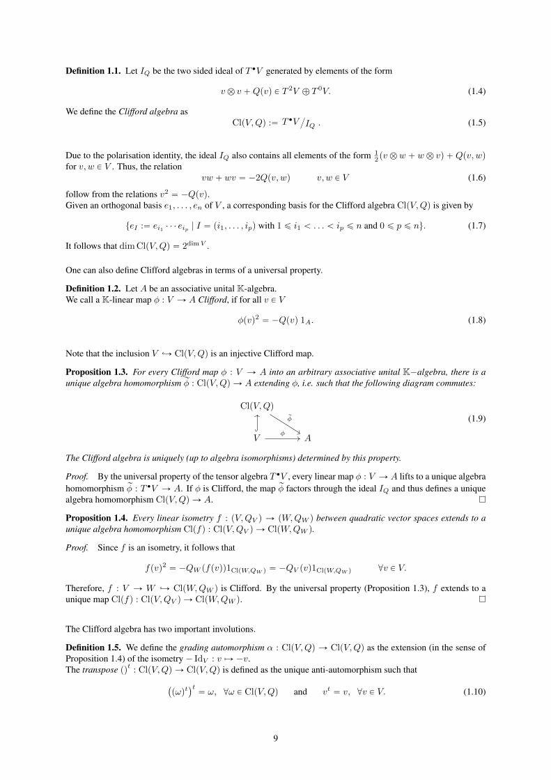
Definition 1.1. Let IQ be the two sided ideal of T ‚V generated by elements of the form

v b v `Qpvq P T 2V ‘ T 0V. (1.4)

We define the Clifford algebra asClpV,Qq :“ T ‚V

L

IQ . (1.5)

Due to the polarisation identity, the ideal IQ also contains all elements of the form 12 pv b w ` w b vq `Qpv, wq

for v, w P V . Thus, the relationvw ` wv “ ´2Qpv, wq v, w P V (1.6)

follow from the relations v2 “ ´Qpvq.Given an orthogonal basis e1, . . . , en of V , a corresponding basis for the Clifford algebra ClpV,Qq is given by

teI :“ ei1 ¨ ¨ ¨ eip | I “ pi1, . . . , ipq with 1 ď i1 ă . . . ă ip ď n and 0 ď p ď nu. (1.7)

It follows that dim ClpV,Qq “ 2dimV .

One can also define Clifford algebras in terms of a universal property.

Definition 1.2. Let A be an associative unital K-algebra.We call a K-linear map φ : V Ñ A Clifford, if for all v P V

φpvq2 “ ´Qpvq 1A. (1.8)

Note that the inclusion V ãÑ ClpV,Qq is an injective Clifford map.

Proposition 1.3. For every Clifford map φ : V Ñ A into an arbitrary associative unital K´algebra, there is aunique algebra homomorphism rφ : ClpV,Qq Ñ A extending φ, i.e. such that the following diagram commutes:

ClpV,Qq

V A

rφ

φ

(1.9)

The Clifford algebra is uniquely (up to algebra isomorphisms) determined by this property.

Proof. By the universal property of the tensor algebra T ‚V , every linear map φ : V Ñ A lifts to a unique algebrahomomorphism rφ : T ‚V Ñ A. If φ is Clifford, the map rφ factors through the ideal IQ and thus defines a uniquealgebra homomorphism ClpV,Qq Ñ A.

Proposition 1.4. Every linear isometry f : pV,QV q Ñ pW,QW q between quadratic vector spaces extends to aunique algebra homomorphism Clpfq : ClpV,QV q Ñ ClpW,QW q.

Proof. Since f is an isometry, it follows that

fpvq2 “ ´QW pfpvqq1ClpW,QW q “ ´QV pvq1ClpW,QW q @v P V.

Therefore, f : V Ñ W ãÑ ClpW,QW q is Clifford. By the universal property (Proposition 1.3), f extends to aunique map Clpfq : ClpV,QV q Ñ ClpW,QW q.

The Clifford algebra has two important involutions.

Definition 1.5. We define the grading automorphism α : ClpV,Qq Ñ ClpV,Qq as the extension (in the sense ofProposition 1.4) of the isometry ´ IdV : v ÞÑ ´v.The transpose pqt : ClpV,Qq Ñ ClpV,Qq is defined as the unique anti-automorphism such that

`

pωqt˘t“ ω, @ω P ClpV,Qq and vt “ v, @v P V. (1.10)

9

Given an orhogonal basis te1, . . . , enu of V with corresponding basis tei1 ¨ ¨ ¨ eip | 1 ď i1 ă . . . ă ip ď nu ofClpV,Qq, the involutions are given by

αpei1 ¨ ¨ ¨ eipq “ p´1qpei1 ¨ ¨ ¨ eip , (1.11)tpei1 ¨ ¨ ¨ eipq “ eip ¨ ¨ ¨ ei1 . (1.12)

Before investigating Clifford algebras more thoroughly, we will briefly give some low dimensional examples.

Example 1.6. Let V “ Rn with the euclidean quadratic form v2 “řni“1 v

2i . We denote the associated Clifford

algebra ClpV, ¨ 2q by Clpnq.For V “ R with unit basis vector i P V , the algebra Clp1q is spanned by the basis t1, iu with relations

i2 “ ´1. (1.13)

Therefore, as real algebras Clp1q – C.For V “ R2 with orthonormal basis i, j P V , the Clifford algebra Clp2q has basis t1, i, j, ku, where k :“ ij andrelations

i2 “ ´1, j2 “ ´1, ij “ ´ji. . (1.14)

This defines the algebra H of quaternions. We have shown that Clp2q – H.

1.1.2 Grading, Filtration and the Symbol Map

In the following section, we focus on the structure of ClpV,Qq inherited by the tensor algebra T ‚V and the innerproduct.

Consider the grading automorphism α : ClpV,Qq Ñ ClpV,Qq from Definition 1.5. Since α2 “ IdClpV,Qq, itfollows that (as vector spaces)

ClpV,Qq “ Cl0pV,Qq ‘ Cl1pV,Qq, (1.15)

whereClipV,Qq “ tu P ClpV,Qq | αpuq “ p´1qiuu. (1.16)

This defines a Z2-grading on ClpV,Qq. Indeed, since α is an algebra homomorphism

ClipV,Qq ¨ CljpV,Qq Ď Cli`j pmod 2qpV,Qq i, j P Z2. (1.17)

We call elements of Cl0pV,Qq even and elements of Cl1pV,Qq odd. This owes to the fact that Cl0pV,Qq is spannedby products of even numbers of elements of V , while Cl1pV,Qq is spanned by an odd number.Observe that Cl0pV,Qq is a subalgebra of ClpV,Qq, whereas Cl1pV,Qq is not.

This Z2-grading is a remnant of the N´ grading of the tensor algebra

T ‚V “à

nPNV bn “

˜

à

n evenV bn

¸

‘

˜

à

n oddV bn

¸

, (1.18)

that factors through the ideal IQ.

Another structure inherited from the grading of the tensor algebra is the filtration of ClpV,Qq. Indeed, since everygraded algebra is trivially a filtered algebra we have the following filtration of T ‚V

FnV :“à

iďn

V bi F0V Ď F1V Ď . . . Ď T ‚V FnV b FmV Ď Fn`mV. (1.19)

Since quotienting by the ideal IQ can only decrease degree, this filtration induces a filtration on the Clifford algebra

Fn ClpV,Qq :“`À

iďn Vbi˘

M

IQ . (1.20)

Recall that every filtered algebra F0A Ď . . . Ď A has an associated graded algebra GpAq “À

nPN GnA withG0A :“ F0A and Gn :“ FnAFn´1A for n ą 0. As a vector space GpAq is isomorphic to A, as algebras theyare usually distinct.

10

Proposition 1.7. The associated graded algebra of ClpV,Qq is the exterior algebra ΛV .

Proof. Indeed, note that

Gn ClpV,Qq “`À

iďn VbiIQ

˘

M

`À

iďn´1 VbiIQ

˘

– V bnL

I “ ΛnV,

where I is the ideal of T ‚V generated by v b v for v P V .

Therefore, the Clifford algebra can be seen as an enhancement of the exterior algebra. Indeed, Clifford inventedhis algebra as a means of incorporating the inner product in the exterior algebra. From the point of view ofphysics, the exterior algebra represents the classical fermionic Fock space with the classical anticommutationrelation ei ¨ ej ` ej ¨ ei “ 0. Quantising this Fock space leads to an algebra with canonical anticommutationrelations ei ¨ ej ` ej ¨ ei “ ~δij . Up to a sign, this is exactly the Clifford algebra. Therefore, the isomorphismΛV Ñ ClpV,Qq is often called quantisation map. This is discussed in greater detail in section 1.4.

Definition 1.8. The isomorphism σ : ClpV,Qq Ñ ΛV is called the symbol map.

Explicitly, its inverse σ´1 : ΛV Ñ ClpV,Qq is given by the linear extension of

v1 ^ ¨ ¨ ¨ vr ÞÑ1

r!

ÿ

σPSr

signpσqvσp1q ¨ ¨ ¨ vσprq v1, . . . , vr P V. (1.21)

Given an orthonormal basis e1, . . . , en of V , this isomorphism maps

ei1 ^ ¨ ¨ ¨ ^ eir ÞÑ ei1 ¨ ¨ ¨ eir , for 1 ď i1 ă . . . ă ir ď n. (1.22)

Since ClpV,Qq and ΛV are isomorphic, we can define an action of ClpV,Qq on the exterior algegra.

Definition 1.9. We define Clifford multiplication of ClpV,Qq on the vector space ΛV by

cpαq :“ σ pα ¨ qσ´1 P EndpΛV q α P ClpV,Qq. (1.23)

From now on we suppose that Q is non-degenerate, such that we have an isomorphism Qp´, ¨q : V Ñ V ˚.

Definition 1.10. We define the interior product ι : V Ñ EndpΛV q as ιpvq “ ιQpv,¨q, where ιω denotes contractionof a covector ω P V ˚ with an element of ΛV . Explicitly,

ιpvqv1 ^ ¨ ¨ ¨ ^ vk “kÿ

i“1

p´1qi`1Qpvi, vqv1 ^ ¨ ¨ ¨ ^ pvi ^ ¨ ¨ ¨ ^ vk. (1.24)

We also define the exterior product ε : V Ñ EndpΛV q by

εpvq :“ v ^ ¨. (1.25)

The interior product ι is adjoint to ε with respect to the quadratic form Q on ΛV ,

Qpεpvqω, ω1q “ Qpω, ιpvqω1q ω, ω1 P ΛV, v P V. (1.26)

Observe that since v ^ v “ 0, it follows that

εpvq2 “ 0, ιpvq2 “ 0, εpvqιpwq ` ιpwqεpvq “ Qpv, wq for v, w P V. (1.27)

We can reexpress Clifford multiplication by vectors in V using interior and exterior product.

Proposition 1.11. For v P V Ď ClpV,Qq we have that

cpvq “ εpvq ´ ιpvq P EndpΛV q. (1.28)

Proof. Let ei1 ^ ¨ ¨ ¨ ^ eik P ΛV , where e1, . . . en is an orthonormal basis for V . Then

cpeiqei1 ^ ¨ ¨ ¨ ^ eik “ σpei ¨ ei1 ¨ ¨ ¨ eikq “

"

ei ^ ei1 ^ ¨ ¨ ¨ ^ eik i R ti1, . . . , ikup´1qjei1 ^ ¨ ¨ ¨ ^ xeij ^ ¨ ¨ ¨ ^ eik i “ ij

.

On the other hand,

pεpeiq ´ ιpeiqqei1 ^ ¨ ¨ ¨ ^ eik “

"

ei ^ ei1 ^ ¨ ¨ ¨ ^ eik i R ti1, . . . , ikup´1qjei1 ^ ¨ ¨ ¨ ^ xeij ^ ¨ ¨ ¨ ^ eik i “ ij

.

11

1.2 The Spin and Pin Groups

We are now ready to introduce the groups Spinn and Pinn as certain multiplicative subgroups of the Cliffordalgebra. As a guiding principle, we will try to find a double cover of SOn and On among these subgroups.

1.2.1 Subgroups of Clpnq

From now on we let V “ Rn with euclidean quadratic form v2 :“řni“1 v

2i and denote the corresponding Clif-

ford algebra ClpRn, ¨ q by Clpnq.In this section we study several (multiplicational) subgroups of the algebra Clpnq, eventually leading to the defini-tion of the Pin and Spin groups.

Since Clpnq is a unital algebra, a first subgroup to consider is the following.

Definition 1.12. The group of units of the algebra Clpnq is

Clˆn :“ tu P Clpnq | Du´1 P Clpnq, s.t. u´1u “ uu´1 “ 1u. (1.29)

Since v ´vv2 “ 1, it follows that an element v P V is invertible, if and only if v ‰ 0.

Having defined a group Clˆn , we could consider its adjoint action on itself, given by Adpuqv“uvu´1 for u,v PClˆn .However, we will use the grading automorphism α from Definition 1.5 to define a slightly different action.

Definition 1.13. The group of units Clˆn acts on Clpnq via the twisted adjoint action

ĂAd : Clˆn Ñ AutpClpnqq ĂAdupxq :“ αpuqxu´1 u P Clˆn , x P Clpnq. (1.30)

This action is well defined since ĂAdu is invertible with inverse ĂAdu´1 and is a group homomorphism since α is.

For v ‰ 0 P Rn and w P Rn, we have that

ĂAdvpwq “ αpvqwv´1 “ ´vw´v

v2“ w ´ 2v

xv, wy

v2P Rn. (1.31)

Thus, we see that ĂAdv : Rn Ñ Rn defines the reflection at the plane orthogonal to the line passing through v. Thisis the reason we considered the twisted adjoint action instead of the adjoint action.However, for a general ω P Clˆn , ĂAdωpRnq Ę Rn.

Definition 1.14. We define the Clifford group

Γn :“ tu P Clˆn |ĂAdupvq P Rn, @v P Rnu (1.32)

as the subgroup of Clˆn that stabilises Rn.

Clearly, any product of non-zero vectors in Rn is contained in Γn. In fact, the Clifford group is the subgroup ofClpnq generated by non-vanishing vectors. Therefore, the maps α and p¨qt restrict to an automorphism and ananti-automorphism on Γn. A proof of this can be found in [6].

By construction, the twisted adjoint representation ĂAd : Clˆn Ñ AutpClpnqq restricts to a representation

ĂAd : Γn Ñ AutpRnq “ Gln . (1.33)

Since Γn is generated by all non-zero vectors in Rn, it follows that its image under ĂAd is the set of all possiblecompositions of reflections. The following lemma thus shows that any composition of reflections is a rotation.

12

Lemma 1.15. The image of ĂAd : Γn Ñ Gln is contained in On.

Proof. Observe that for v P Rn, we have that v2 “ ´v ¨ v “ αpvqv. Thus, for v P Rn, φ P Γn

ĂAdφv2 “ αpĂAdφvqĂAdφv “ φp´vqαpφ´1qαpφqvφ´1 “ ´φv ¨ vφ´1 “ v2.

Since ĂAdφ preserves the norm ¨ , it is an element of On.

We’ve seen that Γn is generated by non-vanishing vectors in Rn and that ĂAd : Γn Ñ On maps such vectors tothe reflection at the plane orthogonal to these vectors. The following theorem from linear algebra guarantees thatevery rotation can be obtained from reflections.

Theorem 1.16 (Cartan-Dieudonné). Every rotation R P On can be written as a product of at most n reflections.

Proof. A proof can be found in [6].

Combining this result with a calculation of the kernel of ĂAd we find the following lemma.

Lemma 1.17. The following is a short exact sequence

1 ÝÑ Rˆ ãÑ ΓnĄAdÝÑ On ÝÑ 1. (1.34)

Proof. By the Cartan-Dieudonné theorem 1.16 every rotation R P On can be written as a product of reflectionsR “ ρv1 ¨ ¨ ¨ ρvr , where ρv denotes reflection at the plane orthogonal to v P Rn.Since ρv “ ĂAdv , it follows that ĂAd : Γn Ñ On is surjective.Let’s compute its kernel. Suppose φ P Γn is in the kernel of ĂAd. Then αpφqv “ vφ. Decomposing φ “ φ` ` φ´,where φ` is even and φ´ is odd we obtain pφ` ´ φ´qv “ vpφ` ` φ´q, or

φ`v “ vφ` φ´v “ ´vφ´ @v P Rn.

Fix an orthonormal basis v1, . . . , vn of Rn.We write φ˘ “ a˘ ` v1b¯, where a˘, b¯ are elements of Clpnq not containing v1 if spanned in terms of the basisof Clpnq associated to the basis v1, . . . , vn of Rn. Observe that a` and b` are even, while a´ and b´ are odd.Therefore, a˘v1 “ ˘v1a˘, b˘v1 “ ˘v1b˘ and we calculate

˘v1a˘ ˘ b¯ “ pa˘ ` v1b¯qv1 “ φ˘v1 “ ˘v1φ˘ “ ˘v1a˘ ¯ b¯.

Therefore, b˘ “ 0. Repeating this argument succesively for all basis vectors, it follows that φ˘ does not containingany vi and is therefore a constant. Since φ˘ P Γn, this constant is non-zero. Thus kerpĂAdq “ Rˆ.

1.2.2 The Groups Pinn and Spinn

So far we have considered the Clifford group Γn generated by all non-zero vectors and have obtained a Rˆ-foldcovering of On. To obtain a double cover, we have to restrict to the group generated by unit vectors.

Definition 1.18. We define the spinor norm N : Clpnq Ñ Clpnq as

N : u ÞÑ uαpuqt. (1.35)

The name ’spinor norm’ comes from the observation that for v P Rn, we have that Npvq “ ´v2 “ v2.However, on arbitrary elements of Clpnq the spinor norm has not much in common with a norm; in general it isn’teven a real number. If we restrict the spinor norm to the Clifford group Γn we can recover its norm-like behaviour.

13

Lemma 1.19. The restriction of the spinor norm N to the Clifford group Γn is a homomorphism

N : Γn Ñ Rˆ (1.36)

such that Npαpxqq “ Npxq, @x P Γn.

Proof. Let x P Γn. Since α and p¨qt restrict to (anti-) automorphism on Γn it follows that αpxqt P Γn. Therefore,Npxq “ xαpxqt P Γn.We will show that ĂAdNpxq “ 1. It then follows from Lemma 1.17 that Npxq P kerpĂAdq “ Rˆ.Let v P Rn. Since xt P Γn, it follows that αpxqtvxt´1

P Rn. Applying p¨qt and observing that wt “ w, @w P Rn,

αpxqtvpx´1qt “ x´1vαpxq.

Therefore,v “ xαpxqtvα

`

xαpxqt˘´1

“ ĂAdαNpxqv “ ĂAdNpxqv.

We can use this norm N to restrict Γn to unit vectors and introduce the groups Pinn and Spinn.

Definition 1.20. We define the pinor group Pinn as the kernel of the homomorphism N : Γn Ñ Rˆ and thespinor group Spinn as its even part PinnXCl0pnq, where Cl0pnq is the even part of the Clifford algebra.Since α|Cl0pnq “ Id, we don’t have to distinguish between adjoint and twisted adjoint for the Spinn group.Therefore,

Pinn “ tx P Clpnq | αpxqvx´1 P Rn, @v P Rn, Npxq “ 1u (1.37)

Spinn “ tx P Cl0pnq | xvx´1 P Rn, @v P Rn, Npxq “ 1u. (1.38)

The group Pinn is the subgroup of Clˆn generated by unit vectors of Rn and Spinn is the subgroup of Pinngenerated by even products of unit vectors of Rn.

Using the spinor normN to restrict the short exact sequence of Γn to unit vectors, we find that the Spinn and Pinngroup are indeed double covers of SOn and On, respectively.

Theorem 1.21. There are short exact sequences

1 ÝÑ Z2 ãÝÑ PinnĄAdÝÑ On ÝÑ 1 (1.39)

1 ÝÑ Z2 ãÝÑ SpinnAdÝÑ SOn ÝÑ 1. (1.40)

Proof. Observe that for k P Rˆ, Npkq “ k2. Thus, the following diagram commutes

1 Rˆ Γn On 1

1 Rˆ Rˆ 1 1

p¨q2

ĄAd

N

“

which means that φ :“ tpq2, N, 1u is a morphism of chain complexes with kernel

1 ÝÑ Z2 ãÝÑ PinnĄAdÝÑ On ÝÑ 1.

Since both domain and codomain of φ are exact, it follows that the above sequence is exact. Restricting to Cl0pnqand observing that the product of an even number of reflections is contained in SOn, it follows that

1 Ñ Z2 ãÝÑ SpinnAdÝÑ SOn ÝÑ 1

is exact.

14

From now on we will focus on the spinor group Spinn.As alluded to in the introduction of this chapter, one can prove that the spin group Spinn is simply connected forn ě 3 and therefore the universal cover of SO3. This explains its appearance in quantum physics.

Example 1.22. We continue Example 1.6 and discuss the Spinn-group and the adjoint map Ad : Spinn Ñ SOn

in the cases n “ 1 and n “ 2.For n “ 1 we have that Clp1q “ spant1, iu – C. The even subalgebra is Cl0p1q “ spant1u – R. The groupSpin1 is the group generated by even products of unit vectors. Thus, Spin1 is the group t1, i2 “ ´1u “ Z2.For n “ 2 with Clp2q “ H “ spant1, i, j, k “ iju we have that Cl0p2q “ spant1, ku with relation

k2 “ ijij “ ´1. (1.41)

Therefore, Cl0p2q – C. Under this isomorphism, for x P Cl0p2q, the map Adx acts as

Adxpvq “x2

|x|2v v P R2 – C,

where | ¨ | denotes the aboslute value in C. Thus, AdxpR2q Ď R2, which implies that

Spin2 “ tx P Cl0p2q | Npxq “ 1u – tx P C | |x|2 “ 1u “ S1, (1.42)

where we have used that Npxq “ xxt “ px1 ` kx2qpx1 ´ kx2q “ xx “ |x|2.Identifying SO2 with S1 acting on C by phase multiplication we thus find that Ad : Spin2 – S1 Ñ SO2 – S1

acts asAd : S1 Ñ S1 z ÞÑ z2. (1.43)

1.2.3 The Lie Algebra spinn

Since Spinn is a subgroup of the algebra Clpnq, it follows that its Lie algebra spinn is a Lie subalgebra of Clpnqwith commutator rα, βs “ α ¨ β ´ β ¨ α. Let σ : Clpnq Ñ ΛRn be the symbol map, the isomorphism between theClifford algebra and the exterior algebra from Definition 1.8.

Lemma 1.23. The Lie algebra spinn is the subalgebra σ´1pΛ2Rnq of Clpnq.

Proof. We will first show that σ´1pΛ2Rnq is indeed a subalgebra of Clpnq.Let e1, . . . , en be an orthonormal basis of Rn, such that σ´1pΛ2Rnq “ spantei ¨ej | i ă ju. A computation showsthat the commutator rei ¨ ej , ek ¨ els is again contained in spantei ¨ ej | i ă ju. Thus, σ´1pΛ2Rnq is a subalgebraof Clpnq.To prove that the subalgebra spinn equals σ´1pΛ2Rnq we consider the curve

γijptq :“ cosptq1` sinptqei ¨ ej P Spinn for i ă j

and observe that γp0q “ 1, 9γp0q “ ei ¨ ej . Thus, the span spantei ¨ ej | i ă ju “ σ´1pΛ2Rnq is contained in theLie algebra spinn.Since Ad : Spinn Ñ SOn is a double cover, it follows that spinn – son. Therefore, dimpspinnq“dimpsonq“

`

n2

˘

.On the other hand, dimpσ´1pΛ2Rnqq “ dimpΛ2Rnq “

`

n2

˘

, which proves that σ´1pΛ2Rnq “ spinn.

The double cover Ad : Spinn Ñ SOn induces an isomorphism Ad˚ : spinn Ñ son.Fix an orthonormal basis e1, . . . , en of Rn. The associated standard basis of son is given by ei N ej P son,

ei N ejpvq :“ xv, ejyei ´ xv, eiyej v P Rn. (1.44)

In matrix notation, every antisymmetric matrix pAijq corresponds to the element

A “ÿ

iăj

Aijei N ej P son. (1.45)

The notation ei N ej is chosen since Λ2Rn Ñ son, ei ^ ej Ñ ei N ej defines an isomorphism of Lie algebras.Using the basis ei N ej of son, we can now describe the isomorphism Ad˚ : spinn “ σ´1pΛ2Rnq Ñ son.

15

Proposition 1.24. Given an orthonormal basis e1, . . . , en P Rn, the isomorphism Ad˚ : spinn Ñ son is given onbasis elements by

Ad˚ : ei ¨ ej ÞÑ ´2ei N ej . (1.46)

Proof. Let γptq “ cosptq1` sinptqei ¨ ej P Spinn. Then Adγptq P SOn is given by

Adγptq v “ γptq ¨ v ¨ γptq´1 v P Rn,

with derivative at the identity

pAd˚ ei ¨ ejq pvq “ pAd˚ 9γp0qq pvq “d

dt

ˇ

ˇ

ˇ

ˇ

t“0

Adγptq v “d

dt

ˇ

ˇ

ˇ

ˇ

t“0

`

γptq ¨ v ¨ γptq´1˘

“ ei ¨ ej ¨ v ´ v ¨ ei ¨ ej .

This equals

rei ¨ ej , vs “ ei ¨ ej ¨ v ` ei ¨ v ¨ ej ` 2xv, eiyej “ 2xv, eiyej ´ 2xv, ejyei “ ´2ei N ejpvq

Given an antisymmetric matrix A “ pAijq P son, we have that

Ad´1˚ A “ Ad´1

˚

˜

ÿ

iăj

Aijei N ej

¸

“ ´1

2

ÿ

iăj

Aijei ¨ ej “ ´1

4

nÿ

i,j“1

Aijei ¨ ej . (1.47)

1.3 Spinor Representations

In the following section we will study representations of the Clifford algebra Clpnq and the spin group Spinn . Wewill see that in even dimensions, the Clifford algebra has exactly one irreducible representations S, called the spinrepresentation. This representation splits in two irreducible Spinn-representations S “ S` ‘ S´.

To deal with representations it is more convenient to consider the complexification of the Clifford algebra

ClCpnq :“ Clpnq b C. (1.48)

Observe that this complexification equals the complex Clifford algebra ClpCn, qq, where q is the (complex-bilinear!) form

qpz, wq :“nÿ

i“1

ziwi z, w P Cn. (1.49)

Definition 1.25. A representation of the Clifford algebra ClCpnq is a C´algebra homomorphism

ρ : ClCpnq Ñ EndCpW q, (1.50)

where W is a finite-dimensional C´vector space.

In Definition 1.9, we have already encountered the representation c : ClCpnq Ñ EndCpΛCnq induced by the map

c : VC Ñ EndpΛCnq cpvq :“ εpvq ´ ιpvq. (1.51)

However, observe that ΛCn is generated by εpvq and ιpvq acting on 1 P ΛCn for v P Cn, while the image ofClCpnq is only generated by cpvq “ εpvq ´ ιpvq. Thus, ClCpnq1 Ď ΛCn is a proper subspace and ΛCn thereforenot an irreducible representation.

However, in the even dimensional case n “ 2m, we can use a similar construction as (1.51) to obtain an irreduciblerepresentation of ClCpnq.

16

Let V “ R2m and let J be a complex structure on V , i.e. a linear map J : V Ñ V such that J2 “ ´1V which iscompatible with the real euclidean product p¨, ¨q in the sense that pJv, Jwq “ pv, wq.Let VC “ V b C be the complexification of V . The euclidean product on V extends to the (complex-bilinear!)form q on VC defined in equation (1.49). The complexification decomposes into

VC “ P ‘ P , (1.52)

where P and P are the `i and ´i eigenspaces of J b 1.The notation P comes from the fact that complex conjugation

¨ : VC Ñ VC, v b µ ÞÑ v b µ v P V, µ P C, (1.53)

restricts to a real isomorphism ¨ : P Ñ P .Since J is compatible with the euclidean product p¨, ¨q, it follows that

qpp1, p2q “ 0 “ qpb1, b2q p1, p2 P P, b1, b2 P P . (1.54)

and that q places P and P in duality, i.e. such that the map

P Ñ P˚ b ÞÑ qpb, ¨q (1.55)

is an isomorphism. The choice of subspace P is known as a polarisation of VC.

On the complex vector space VC with bilinear form q, we define the exterior product ε : VC Ñ EndCpΛVCq andinterior product ι : VC Ñ EndCpΛVCq as in Definition 1.10.Observe that for p P P , b P P we have that

εppq P EndCpΛP q and ιpbq P EndCpΛP q. (1.56)

We define the map c : VC Ñ EndCpΛP q as

cpp` bq :“?

2 pεppq ´ ιpbqq , p` b P VC “ P ‘ P . (1.57)

It squares tocpp` bq2 “ 2

`

εppq2 ´ εppqιpbq ´ ιpbqεppq ` ιpbq2˘

. (1.58)

Using relations (1.27), it follows that

cpp` bq2 “ ´2qpp, bq “ ´qpp` b, p` bq. (1.59)

Thus, the map c : VC Ñ EndCpΛP q is Clifford and induces a map

c : ClpVC, qq “ ClCp2mq Ñ EndCpΛP q. (1.60)

For different choices of complex structure J we get different polarisations P . However, one can prove that therepresentations c : ClCp2mq Ñ EndCpΛP q are equivalent. For definiteness, we let S :“ ΛP , where P is the

subspace of C2m obtained from the standard complex structure J “ˆ

0 ´1m

1m 0

˙

on R2m. Explicitly,

P “ spantej ´ i ej`m | 1 ď j ď mu and P “ spantej ` i ej`m | 1 ď j ď mu, (1.61)

where e1, . . . , e2m is the standard basis of R2m.

We observe that dimpSq “ 2m.

Definition 1.26. The representation c : ClCp2mq Ñ EndCpSq is called the spin representation.The 2m´dimensional space S is the spin space.

Usually, the map c : ClCp2mq Ñ EndCpSq is called Clifford multiplication.

17

Proposition 1.27. The representationc : ClCp2mq Ñ EndCpSq (1.62)

is an isomorphism of C´algebras and thus irreducible.

Proof. We start by proving that c is surjective.Let V “ R2m, VC “ C2m and P, P as in 1.52. The algebra EndCpSq “ EndCpΛP q is generated by εppq for p P Pand ιω for ω P P˚. The complex bilinear form q induces an isomorphism between P˚ and P (equation (1.55))such that for every ω P P˚, there is a b P P with ιω “ ιpbq. Since cppq “

?2εppq and cpbq “ ´

?2ιpbq “ ´

?2ιω ,

it follows that c is surjective.It is an isomorphism, since dimCpClCp2mqq “ 22m and dimCpEndCpSqq “ p2

mq2“ 22m.

It is proven in [6], that in even dimension n “ 2m, the spin space S is up to equivalence the unique irreducibleClCp2mq´representation.

Proposition 1.28. There exists a hermitian product x¨, ¨y on S such that

xcpvqs, s1y “ ´xs, cpvqs1y @s, s1 P S, v P R2m Ď C2m. (1.63)

Proof. We define the inner product on S using our explicit construction of S “ ΛP from above.It suffices to define an hermitian product with properties (1.63) on P , which can then be extended to ΛP .Let ¨ : P Ñ P denote complex conjugation. We define the hermitian product

xp, p1y :“ qpp, p1q p, p1 P P. (1.64)

Let v P V “ R2m. Since v is real, it is of the form v “ w ` w for some w P P . Thus, cpvq “?

2 pεpwq ´ ιpwqqand

xcpvqp, p1y “?

2xpεpwq ´ ιpwqqp, p1y “?

2q`

εpwq ´ ιpwqp, p1˘

.

Since ι is adjoint to ε with respect to q (equation 1.26), it follows that

xcpvqp, p1y “?

2 q´

p,`

ιpwq ´ εpwq˘

p1¯

“ ´?

2 q´

p,`

εpwq ´ ιpwq˘

p1¯

“ ´xp, cpvqp1y.

If we restrict this representation of ClCp2mq to the Spin group, we obtain a representation of Spin2m.

Definition 1.29. The complex spin representation of Spin2m is the homomorphism

πS : Spin2m Ñ GlCpSq, (1.65)

obtained by restricting the irreducible spin representation of ClCp2mq to Spin2m Ď Cl0p2mq Ď ClCp2mq.

Using equation (1.63) and the fact that Spinn is generated by an even number of unit vectors in Clpnq, we see thatthe spin representation πS is unitary with respect to the hermitian product x¨, ¨y on S.

The representation πS is not irreducible. This can be seen by the following.

Definition 1.30. We define the complex volume element ωC P ClCp2mq as

ωC :“ ime1 ¨ ¨ ¨ e2m, (1.66)

where e1, . . . , e2m is a positively oriented orthonormal basis of R2m.

A calculation shows that ω2C “ 1. Thus, we can split every ClCp2mq-representation W into a direct sum of ˘1

eigenspaces of ωC, i.e.

W “W` ‘W´, W˘ :“1

2

`

1˘ ρpωCq˘

W. (1.67)

Noticing thatωCα “ αωC for all α P Cl0Cp2mq, (1.68)

we see that each ofW˘ is invariant under the even subalgebra Cl0Cp2mq and defines a subrepresentation for Cl0Cp2mq.

18

Given the spin representation S, we can therefore decompose S “ S` ‘ S´ in Spin2m-subrepresentations.In terms of our explicit construction S “ ΛP , these subrepresentations are S` “ ΛevenP and S´ “ Λ oddP .The Spin2m representations S` and S´ are inequivalent and irreducible. In fact, they are up to equivalence theonly irreducible Spin2m representations. A proof of these facts can be found in [6].

Definition 1.31. The complex irreducible unitary representations πS˘ : Spin2m Ñ GlCpS˘q are called half spin

representations.

With respect to the hermitian product x¨, ¨y from Definition 1.28, the spaces S` and S´ are orthogonal to eachother.

Example 1.32. Continuing Example 1.6 and 1.22, we discuss the spinor representation of Spin2 – S1.

Consider R2 with the standard complex structure J “ˆ

0 ´11 0

˙

. Then R2 b C “ C2 “ P ‘ P , where

P “ spantf :“ 1?2pe1 ´ ie2qu and P “ spantf :“ 1?

2pe1 ` i e2qu and where e1, e2 is the standard basis of R2.

The spin space is then S “ ΛP “ C‘ P . We decompose

e1 “1

2pe1 ´ ie2q `

1

2pe1 ` ie2q “

1?

2f `

1?

2f and e2 “

i

2pe1 ´ ie2q ´

i

2pe1 ` ie2q “

i?

2pf ´ fq (1.69)

and obtain that c : ClCp2q Ñ EndCpSq “ EndCpC‘ spantfuq is given as the complex linear extension of

cpe1qpa` b fq “`

εpfq ´ ιpfq˘

pa` b fq “ ´b` a f (1.70)

cpe2qpa` b fq “ i`

εpfq ` ιpfq˘

pa` b fq “ ib` ia f. (1.71)

Here, we have used that ιpfqf “ qpf, fq “ 1.The half spin spaces are S` “ ΛevenP “ C “ spant1u and S´ “ ΛoddP “ P “ spantfu.The spin representation πS is given by Clifford multiplication restricted to Spin2.Therefore, for cospφq ` sinpφqe1e2 P Spin2,

πS

´

cospφq ` sinpφqe1e2

¯

pa` b fq “´

cospφq ´ i sinpφq¯

a`´

cospφq ` i sinpφq¯

b f. (1.72)

Identifying S1 – Spin2 via eiφ ÞÑ cospφq ` sinpφqe1e2 and S “ S` ‘ S´ “ spant1u ‘ spantfu – C‘ C, wefind that

πS` : S1 Ñ EndCpCq z ÞÑ z´1 (1.73)

πS´ : S1 Ñ EndCpCq z ÞÑ z (1.74)

πS : S1 Ñ EndCpC2q z ÞÑ

ˆ

z´1 00 z

˙

. (1.75)

1.4 Fermions and Bosons

When we discussed the isomorphism between Clifford algebra and exterior algebra, we mentioned that the Cliffordalgebra can be seen as representing the canoncial anticommutation relations (CARq.The usual presentation of the CAR algebra describing a quantum mechanical system of fermions with n degrees offreedom is slightly different. It is generated by position operators q1, . . . , qn and momentum operators p1, . . . , pnwith relations

qiqj ` qjqi “ 0, pipj ` pjpi “ 0, qipj ` pjqi “ ´δij 1 ď i, j ď n, (1.76)

(modulo a factor of ´i~). However, this algebra is equivalent to the complex Clifford algebra ClCp2nq in 2ngenerators. In fact, choosing a polarisation of R2n, e.g.

pR2nqC p– C2nq “ P ‘ P “ spantej ´ iej`n | 1 ď j ď nu ‘ spantej ` iej`n | 1 ď j ď nu (1.77)

(where e1, . . . , e2n is an ONB of R2n, see (1.61)), we find that the Clifford algebra ClCp2nq is generated by vectorsqi “

12 pei ´ iej`nq and pi “ 1

2 pei ` iei`nq with relations

qiqj ` qjqi “ 0 pipj ` pjpi “ 0 qipj ` pjqi “ ´δij 1 ď i, j ď n. (1.78)

19

Therefore, the Clifford algebra ClCp2nq is in fact equivalent to the CAR algebra.

Completely analogously, we can consider the canonical commutation relations (CCR)

qiqj ´ qjqi “ 0 pipj ´ pjpi “ 0 qipj ´ pjqi “ ´δij 1 ď i, j ď n, (1.79)

describing a system of bosons with n degrees of freedom. Similar to the Clifford algebra, there is a coordinateindependent definition of this algebra.Let V be an even dimensional complex vector space with a symplectic form ω (i.e. an antisymmetric non-degenerate bilinear form ω : V ˆ V Ñ C). We define the Weyl algebra

WpV, ωq :“ T ‚V Iω , (1.80)

where T ‚V is the tensor algebra and Iω is the ideal generated by v b w ´ w b v ` ωpv, wq1 for v, w P V .Observe that in contrary to the Clifford algebra, the Weyl algebra is only defineable in even dimensions.Similar to (1.54), we define a polarisation of V with respect to ω to be a choice of subspaces V “ Q‘P such that

ωpq1, q2q “ 0 “ ωpp1, p2q @q1, q2 P Q, p1, p2 P P. (1.81)

Choosing a basis q1, . . . , qn of Q and p1 . . . pn of P such that ωpqi, pjq “ δij , the Weyl algebra is generated bythe relations

qiqj ´ qjqi “ 0 pipj ´ pjpi “ 0 qipj ´ pjqi “ ´ωpqi, pjq “ ´δij . (1.82)

Therefore, the Weyl algebra is equivalent to the CCR-algebra describing a bosonic system with n degrees offreedom.

We can transfer all results obtained for the Clifford algebra to corresponding results for the Weyl algebra.While the Clifford algebra is a quantisation of the exterior algebra ΛV (i.e. ΛV is the associated graded algebra tothe filtered algebra ClpV q), the Weyl algebra is a quantisation of the symmetric algebra SympV q.The Clifford algebra ClCp2nq is defined via an inner product and therefore related to the group SO2n. In the sameway, the Weyl algebra is defined via a symplectic form and is related to the symplectic group Sp2n.For example, we found in Lemma 1.23 that the quadratic elements σ´1pΛ2C2nq of the Clifford algebra are canon-ically isomorphic to the Lie algebra of the Spin group Spin2n (here, σ : ClCp2nq Ñ ΛC2n is the symbol map).Analogously, we can show that the quadratic elements µ´1pSym2 C2nq of the Weyl algebra Wp2nq are canonicallyisomorphic to the Lie algebra of the double cover of the symplectic group (here µ : Wp2nq Ñ SympC2nq is theisomorphism between symmetric and Weyl algebra). This double cover of the symplectic group is known as themetaplectic group Mp2n.

We can push these analogies between Clifford and Weyl algebra much further. The idea to treat fermions andbosons - or Clifford and Weyl algebra - on a completely equal footing is called supersymmetry.

The utility of supersymmetry becomes apparent if we consider the bosonic analogon of Clifford multiplication (thespin representation) c : ClCp2nq Ñ EndCpSq from Definition 1.27.Following equation (1.57), we define the representation e : Wp2nq Ñ EndCpSymQq as the extension of

e : C2n “ Q‘ P Ñ EndCpSymQq epq ` pq :“ τpqq ` κppq, (1.83)

where τ : QÑ EndCpSymQq is the symmetric product with elements of Q and κ its formal adjoint.Observe that in comparison to (1.57), we ommited a factor

?2, which is due to the missing factor of 2 in the

defining relation v b w ´ w b v “ ´ωpv, wq1 of the Weyl algebra.

The algebra SymQ is the algebra of polynomial expressions in vectors of Q (e.g. q21 ` q2) and can thus be

identified with the algebra CrQ˚s of polynomial functions on the vector space Q˚. Fixing a basis q1, . . . , qn ofQ, this yields an identification SymQ – Crq1, . . . , qns. Under this identification, the symmetric product τpqqbecomes multiplication with q, such that

epqiq : Crq1, . . . , qns Ñ Crq1, . . . , qns pepqiqfq pq1, . . . , qnq “ qifpq1, . . . , qnq. (1.84)

A computation shows that the formal adjoint κppiq corresponds to the derivative with respect to qi, such that

eppiq : Crq1, . . . , qns Ñ Crq1, . . . , qns peppiqfq pq1, . . . , qnq “Bf

Bqipq1, . . . , qnq. (1.85)

20

Since epqiqeppjq´eppjqepqiq “ ´ BqiBqj “ ´δij “ ´ωpqi, pjq, this indeed defines a representation of the Weyl algebra.In the same way as the spinor representation S is the unique irreducible representation of the Clifford algebra, therepresentation e : Wp2nq Ñ EndpCrq1, . . . , qnsq is the unique irreducible representation of the Weyl algebra - afact known as the Stone-von Neumann theorem.

Therefore, in the same way that fermions are represented by Clifford multplication on spinors, bosons correspondto (polynomial) differential operators on Q. The power of supersymmetry is that it relates these two concepts.

In the following, we will mainly focus on fermions and spinors and come back to the idea of supersymmetry onlyin the final step of the proof of the index theorem.

1.5 Spin Geometry

Having discussed algebraic properties of Clifford algebras and spin groups we can now place them in a geometricalcontext.

1.5.1 Differential Geometry

In the following, we will briefly recapitulate important concepts from differential geometry.Let M be a smooth manifold. For a vector bundle E , we denote its space of sections by ΓpEq.

Definition 1.33. Let G be a Lie group. A principal G´bundle PG ÑM over M is a G´fibre bundle with a freeand transitive right action of G on PG which preserves fibres.

The main example of a (Glr ´)principal bundle is the frame bundle PGlrE of a rank r vector bundle E . Its fibrepPGlr pEqqx at x PM is given by the set of all ordered bases of Ex with Glr acting on them by change of basis.

To every principal G´bundle and every G-representation, we can associate a vector bundle.

Definition 1.34. Given a principal G´bundle PG Ñ M and a representation ρ : G Ñ GlpV q we define theassociated vector bundle

PG ˆρ V :“ pPG ˆ V qL

„ , (1.86)

where pp.g, vq „ pp, ρpgqvq, @g P G.

Every rank r vector bundle E is associated to its frame bundle under the fundamental representation

ρ :“ Id : Glr Ñ GlpRrq “ Glr . (1.87)

All other bundles usually associated to E can be reconstructed as associated to its frame bundle. For example,

E “ PGlr pEqˆρRr, E˚ “ PGlr pEqˆρ˚Rr, ΛkE “ PGlr pEqˆΛkρ

`

ΛkRr˘

, bkE “ PGlr pEqˆbkρ`

bkRr˘

,

where ρ˚, Λkρ, br ρ are the induced dual, exterior power and tensor product representations.

Let E be a rank r vector bundle with transition functions φij : UiXUj Ñ Glr and let G Ď Glr. We say that E hasa G´structure, if its transition functions can be chosen to map into G, i.e. if φij : Ui X Uj Ñ G Ď Glr .For example, if E is orientable its transition functions can be chosen to lie in Gl`r . Similarly, if E has an innerproduct, then they can be chosen to lie in Or. We can then consider its oriented or orthonormal frame bundlePGl`r

pEq or POr pEq of oriented or othonormal frames, respectively. This can be generalised to arbitrary principalbundles.

21

Definition 1.35. Let PG Ñ M be a principal G-bundle over a manifold M and let H φÑ G be a group homo-

morphism. The bundle PG reduces/lifts along φ if there exists a trivialisation tUiu of PG with transition mapsgij : Ui XUj Ñ G, such that there exist maps Gij : Ui XUj Ñ H fulfilling the cocycle condition Gij “ GikGkj(i.e. such that they also define a bundle) and such that gij “ φpGijq.The principal bundle PH induced by the transition functions Gij is called a reduction/lift of PG along φ.

If PH is a reduction/lift of PG along φ : H Ñ G, then there exists a bundle map ξ : PH Ñ PG, such that

ξpp.hq “ ξppq.φphq @h P H. (1.88)

In most cases H Ñ G is taken to be an inclusion of a subgroup, which is why we usually speak about a reductionof a G´bundle. However, in the following essay we will be considering the double cover Spinn Ñ SOn, whichmakes it more natural to talk about a lift of the structure group.

Many geometrical notions can be restated in terms of reductions of specific principal bundles.A Riemannian structure on a manifold Mn is defined to be a reduction of its frame bundle PGlnpTMq alongthe inclusion On ãÑ Gln. Each Riemannian structure corresponds to a choice of a specific (isometry class of)Riemannian metrics on TM .An orientation of M is a reduction of the frame bundle PGlnpTMq along Gl`n ãÑ Gln. If such a reduction exists,we say that M is orientable.

Example 1.36. To prepare for our discussion of the existence of spin structures, we briefly investigate the notionof orientability of a manifold M . Consider the short exact sequence

1 Ñ Gl`n ãÑ GlnsignpdetqÑ Z2 Ñ 1. (1.89)

This induces a long exact sequence in cohomology

H1pM,Gl`n q Ñ H1pM,Glnqw1Ñ H1pM,Z2q. (1.90)

We use Cech-cohomology to identify isomorphism classes of principal G-bundles with H1pM,Gq. A principalGln-bundle P is orientable if it reduces to a Gl`n -bundle, i.e. if it lies in the image of H1pM,Gl`n q Ñ H1pM,Glnq.By exactness of (1.90), we have thus obtained that a principal Gln´bundle is orientable if and only if w1pP q “ 0.The class w1pP q P H1pM,Z2q is called the first Stieffel-Whitney class of P .

A local section s : U Ñ P of a principal bundle P yields trivialisations of P and all its associated bundles over U .Indeed, the map px, gq ÞÑ spxq.g identifies UˆG – P |U , trivialising P . Given an associated bundle E “ PˆρRr,the map px, vq ÞÑ rpspxq.g, vqs “ rpspxq, ρpgqvqs identifies U ˆ Rr – E |U .In particular, every local section s : U Ñ P induces a local frame for every associated bundle.

One of the main advantages of the use of principal bundles is to facilitate the study of connections.

Definition 1.37. A covariant derivative on a vector bundle E ÑM is a map

∇ : ΓpEq Ñ ΓpT˚M b Eq, (1.91)

fulfilling the Leibniz rule

∇pfXq “ df bX ` f∇X f P C8pMq, X P ΓpEq. (1.92)

Given a local frame pe1, . . . , erq of E |U , we define the connection one-form as the r ˆ r matrix of one-formsrωij P Ω1pUq such that

∇ei “rÿ

k“1

rωki b ek. (1.93)

The connection one-forms rω P Ω1pU,EndpRrqq “ Ω1pU, glrq are only locally defined and depend on the specifictrivialisation of E |U . Using principal bundles we can organise them into globally defined one-forms independentof the trivialisation.

22

Definition 1.38. A principal connection on a principal G´bundle P Ñ M is an element ω P Ω1pP, gq fulfillingseveral technical conditions, given for example in [2].

Let ω P Ω1pP, gq be a principal connection on P and let E be a vector bundle associated to P via a representationρ : GÑ Glr. We define a covariant derivative on E as follows.Let U Ď M be an open subset and s : U Ñ P be a local section of P trivialising P and inducing a local framee1, . . . , en of E |U .Then s˚ω P Ω1pU, gq and we define rω :“ ρ˚s

˚ω P Ω1pU, glrq, where ρ˚ : gÑ glr is the tangent map of ρ. Thisdefines local connection forms rωij “ ei prωejq and a covariant derivative

∇ “ d` rω : C8pU,Rrq Ñ Ω1pU,Rrq. (1.94)

One can prove that this definition of ∇ is independent of the choice of trivialisation.

We can now define the notion of curvature of a connection.

Definition 1.39. Given a covariant derivative ∇ on a vector bundle E , we define its curvature tensorK∇ P Ω2pM,EndpEqq by

K∇pX,Y q “ r∇X ,∇Y s ´∇rX,Y s X,Y P ΓpTMq. (1.95)

Given a local frame e1, . . . , er over U ĎM , we can trivialise K∇ to obtain the local curvature formK∇U P Ω2pU, glrq defined by

`

K∇U pX,Y q

˘i

j“ ei

`

K∇pX,Y qej˘

X,Y P ΓpTM |U q (1.96)

Having defined the curvature of a covariant derivative, we can define the associated notion for a principal connec-tion ω on a principal bundle.

Definition 1.40. Given a principal connection ω P Ω1pP, gq on a principal bundle P ÑM , we define its principalcurvature

Ωω “ dω ` ω ^ ω P Ω2pP, gq. (1.97)

Let E be a vector bundle associated to P via a representation ρ : G Ñ Glr and let ω be a principal connection onP with induced covariant derivative ∇ on E . Let U Ď M be an open subset and s : U Ñ P be a local section ofP trivialising P |U and E |U with induced local frame e1, . . . , en of E .In this trivialisation we have that s˚Ωω P Ω2pU, gq is related to the trivialised curvature K∇

U P Ω2pU, glnq by

ρ˚ps˚Ωωq “ K∇

U . (1.98)

We will now focus on the tangent bundle TM of a Riemannian manifold pM, gq.The Levi-Civita connection ∇ on ΓpTMq is the unique connection that is torsion free, i.e. such that

∇XY ´∇YX “ rX,Y s for all X,Y P ΓpTMq (1.99)

and compatible with the metric

ZgpX,Y q “ gp∇ZX,Y q ` gpX,∇ZY q for all X,Y, Z P ΓpTMq. (1.100)

Its curvature tensor R P Ω2pM,EndpTMqq is the Riemann curvature tensor. Given a local frame e1, . . . , en ofTM |U , we let

Rijkl “ pRU pei, ejqq

kl “ ekpRpei, ejqelq. (1.101)

Usually, we lower the index k using the metric and define

Rijkl “ÿ

r

grkRijrl “ gpek, Rpei, ejqelq where grk “ gper, ekq. (1.102)

23

The Riemann curvature tensor has the following symmetries:

Rijkl `Rijlk “ 0, (1.103)Rijkl `Rjikl “ 0, (1.104)Rijkl ´Rklij “ 0, (1.105)

Rijkl `Riklj `Riljk “ 0. (1.106)

The last identity is known as the Bianchi identity.We define the Ricci tensor as the contraction of the Riemann tensor Ricij :“

řnk“1 g

klRikjl. The symmetries ofthe Riemann tensor imply that the Ricci tensor is symmetric; Ricij “ Ricji.Finally, we define the scalar curvature of M as

rM :“ÿ

i,j

Ricij gij “

ÿ

ilk

Rikilgkl. (1.107)

This is clearly independent of the local frame and defines a global function rM P C8pMq.

1.5.2 Spin Manifolds

In the following let pMn, gq be an n´dimensional oriented Riemannian manifold. We denote its positively orientedorthonormal coframe bundle by P˚SOn

.

Definition 1.41. A spin structure P˚Spinnon an oriented Riemannian manifold pMn, gq is a lift of P˚SOn

to aprincipal Spinn-bundle along the double cover Ad : Spinn Ñ SOn. An oriented Riemannian manifold with aspin structure is called a spin manifold. We denote the induced bundle map by ξ : P˚Spinn

Ñ P˚SOn.

In the literature, spin structures are either defined as a lift of the frame bundle PSOn (as for example in [6]) or ofthe coframe bundle (see [2]). Here, we have chosen the coframe appraoch to avoid the exterior algebra ΛTM infavour of the much more geometrical ΛT˚M .Since the metric g induces a canonical isomorphism between TM and T˚M , both definitions are equivalent.

Similar to our discussion of orientability in Example 1.36, we can find topological obstructions to the existence ofspin structures. Let’s consider the exact sequence

1 Ñ Z2 ãÑ SpinnAdÑ SOn Ñ 1 (1.108)

with induced long exact sequence

H1pX,SpinnqAdÑ H1pX,SOnq

w2Ñ H2pX,Z2q. (1.109)

Thus, the oriented orthonormal coframe bundle P˚SOnlies in the image of Ad if and only if w2pP

˚SOn

q “ 0.This shows that a manifold M admits a spin structure if and only if the second Stieffel Whitney class of its tangentbundle w2pTMq vanishes.

Definition 1.42. Let Mn“2m be an even dimensional spin manifold. We define the (complex) spinor bundle S asthe associated bundle

S :“ P˚SpinnˆπS S, (1.110)

where πS : Spinn Ñ GlCpSq is the spin representation. Its (local) sections are called spinors.The halfl spinor bundles S˘ are defined as S˘ :“ P˚Spinn

ˆπS˘ S˘ with sections called half spinors.

As vector bundles S decomposes as the direct sum S “ S`‘ S

´. The hermitian product on S induces a hermitianmetric on S with respect to which the bundles S˘ are orthogonal.

Having defined a spinor bundle it is a natural next step to ask for a bundle of Clifford algebras acting on S.

24

To define such a bundle, we observe that any orthogonal transformationR P On induces a map of the tensor algebrato itself which preserves the ideal generated by v b v ` qpvq. Therefore, it induces an orthogonal transformationClpRq on Clpnq (see Proposition 1.4). This defines a representation

Cl : SOn Ñ AutpClnq. (1.111)

Definition 1.43. Let pMn, gq be an n´dimensional oriented Riemannian manifold. We define the Clifford bundleon M to be the associated bundle

ClpMq :“ P˚SOn ˆCl Clpnq. (1.112)

The Clifford bundle has fibres ClpMqx over x PM given by the Clifford algebra ClpT˚xMq associated to T˚xM .We note that in contrast to the spinor bundle, we do not need a spin structure on M to define a Clifford bundle.

We define the complex Clifford bundle as the complexification ClCpMq :“ ClpMq b C.

Definition 1.44. We define the symbol map

σ : ClpMq Ñ ΛT˚M (1.113)

as the vector bundle isomorphism induced by the fibrewise symbol maps σx : ClpT˚xMq Ñ ΛT˚xM from Defini-tion 1.8.

Proposition 1.45. LetMn“2m be an even dimensional spin manifold with spinor bundle S. Clifford multiplicationc : ClCpnq Ñ EndCpSq induces an algebra-bundle (iso)morphism

c : ClCpMq Ñ EndCpSq. (1.114)

Proof. A proof can be found in [6].

As in equation (1.67) we can use a volume form in ClCpMq to define the projections of S to S˘ in terms of Cliffordmultiplication.

Definition 1.46. For an even dimensional spin manifold Mn“2m with volume form ω P ΓpΛnT˚Mq induced bythe metric, we let ωC :“ i

n2 σ´1pωq P ΓpClCpMqq be the complex volume form.

We then obtain thatS˘“`

1 S ˘ cpωCq˘

S. (1.115)

1.5.3 Spin Connection

Since the Levi-Civita connection on M is compatible with the Riemannian structure it defines a principal con-nection τ P Ω1pP˚SOn

, sonq on P˚SOn. Under the spin structure ξ : P˚Spinn

Ñ P˚SOn, τ lifts to a connection

τ 1 “ ξ˚τ P Ω1pP˚Spinn, spinnq on P˚Spinn

.

Definition 1.47. LetMn“2m be an even dimensional spin manifold with Levi-Civita connection τ and let τ 1 “ ξ˚τbe the lift of τ to P˚Spinn

. The induced covariant derivative

∇ S : ΓpSq Ñ ΓpT˚M b Sq (1.116)

is called spin connection.

Trivialised by a local orthonormal frame pe1, . . . , enq of TM |U we can write the Levi-Civita connection on TMas

∇Bi “ Bi ` Γi : C8pU,Rnq Ñ C8pU,Rnq, (1.117)

25

where Γi :“ ΓpBiq and Γ P Ω1pU, sonq are the Christoffel symbols, the local one-form of the Levi-Civita connec-tion. In terms of our frame, they are given by pΓiq

αβ “ eα p∇Bieβq “ g peα,∇Bieβq .

Since gpeα,∇Bieβq “ ´gpeβ ,∇Bieαq, it follows that Γi P son. Using the basis ei N ej of son introduced inequation (1.44), we can write them as

Γi “nÿ

α,β“1

pΓiqαβeα b e

β “ÿ

αăβ

pΓiqαβeα N eβ . (1.118)

Lets compare this to the spin connection ∇ S .The (dual of the) local orthonormal frame s “ pe1, . . . , enq defines a local section of P˚SOn

. Using this section, wecan relate the principal Levi-Civita connection τ to the Christoffel symbols Γ, via

Γ “ ´s˚τ, (1.119)

where the minus comes from the fact that τ defines a connection on the cotangent bundle.Let rs be a section of P˚Spinn

such that ξprsq “ s (since ξ is a double cover, there are two sections with this property).This section rs trivialises P˚Spinn

and therefore also S. In this trivialisation, the local connection one-form of the

spin-connection is Γ S “ πS˚rs˚τ 1 P Ω1pU, glpSqq, where τ 1 P Ω1pP˚Spinn

, spinnq is the lift of the Levi-Civitaconnection and πS : Spinn Ñ GlCpSq is the spin representation. Since τ 1 “ ξ˚τ , it follows that

Γ S “ πS˚rs˚ξ˚τ “ πS˚Ad´1

˚ pξ ˝ rsq˚τ “ πS˚Ad´1

˚ s˚τ “ pπS ˝Ad´1q˚p´Γq, (1.120)

where Ad : Spinn Ñ SOn and we have used that rs˚ξ˚ “ Ad´1˚ pξ ˝ rsq

˚ : Ω1pP˚SOn, sonq Ñ Ω1pU, spinnq.

By definition, the map πS : Spinn Ñ GlCpSq is simply the restriction of Clifford multiplicationc : ClCpnq Ñ EndCpSq to Spinn, such that

∇ SBi“ Bi ` Γ

Si “ Bi ´ c

`

Ad´1˚ pΓiq

˘

. (1.121)

Writing Γi “ř

jăk pΓiqjkej N ek and using (1.47), it follows that

ΓSi “ ´

1

4

nÿ

α,β“1

pΓiqαβcpe

αqcpeβq.

Ommiting the local coordinate system xi of M , we summarise our findings in the following proposition.

Proposition 1.48. Let e1, . . . , en be a local orthonormal frame of TM |U . Let s “ pe1, . . . , enq be the corre-sponding local section of P˚SOn

and let rs be a local section of P˚Spinnin the preimage of s under the spin structure

ξ : P˚SpinnÑ P˚SOn

(there are two choices ˘rs for rs). In the trivialisation of S induced by rs we have that

∇ S “ d`1

4

nÿ

α,β“1

pΓqαβcpe

αqcpeβq where pΓqαβ “ gpeα,∇eβq P Ω1pUq. (1.122)

With a completely analogous discussion we can relate the trivialised curvature of the Levi-Civita connection to thecurvature of the spin connection.

Proposition 1.49. Let e1, . . . , en be a local orthonormal frame of TM |U .The curvature of the spin connection R S P Ω2pM,EndpSqq is

R Spei, ejq “ ´1

4

nÿ

k,l“1

Rijkl cpekqcpelq “ ´

1

2

ÿ

kăl

Rijklcpekqcpelq where Rijkl “ gpek, Rpei, ejqelq (1.123)

and where R P Ω2pM,EndpTMqq is the Riemann curvature tensor.

Proof. This proof is very similar to the proof of the previous proposition. Let s and rs be as in Proposition 1.48.Let Ωτ P Ω2pP˚SOn

, sonq be the principal curvature of the Levi-Civita connection τ , such that the local curvature(see equation (1.96)) is RU “ s˚Ωτ P Ω2pU, sonq.

26

We use the basis (1.44), to write RU pX,Y q “ř

αăβ pRU pX,Y qqαβeα N eβ .

By formula (1.98), R SU “ πS˚rs˚Ωτ

1

, where πS : Spinn Ñ GlCpSq is the spin representation and τ 1 is the spinconnection. Since τ 1 “ ξ˚τ , it follows that Ωτ

1

“ ξ˚Ωτ and thus that R SU “ πS˚rs˚Ωτ

1

“ πS˚Ad´1˚ pRU q.

Therefore,

RSU pX,Y q “ ´

1

4

nÿ

α,β“1

RU pX,Y qαβcpe

αqcpeβq.

The claim follows, since RU pei, ejqαβ “ eαpRpei, ejqeβq “ gpeα, Rpei, ejqeβq “ Rijαβ .

Since ClCpMq is associated to P˚SOn, the Levi-Civita connection induces a connection ∇ on ClCpMq. The spin

connection is compatible with the structure on S defined so far.

Proposition 1.50.

(1) The spin connection ∇ S is compatible with the hermitian product p¨, ¨q on S, in the sense that

Xps, s1q “ p∇ SXs, s

1q ` ps,∇`X Ss1q P T˚M s, s1 P ΓpSq, X P ΓpTMq. (1.124)

(2) The spin connection ∇ S is compatible with Clifford multiplication in the sense that

∇ SXpcpαqsq “ cp∇Xαqs` cpαq∇ S

Xs X P TM, s P ΓpSq, α P ΓpClCpMqq. (1.125)

Proof. A proof can be found in [6].

Having discussed the spin connection, we can now define the central object of this essay.

Definition 1.51. The Dirac operator D on an even dimensional spin manifold Mn“2m is the operator

D : ΓpSq∇ S

ÝÑ ΓpT˚M b SqcÝÑ ΓpSq. (1.126)

Given a local orthonormal frame e1, . . . , en of TM |U with corresponding dual frame e1, . . . , en of T˚M |U , theDirac operator can be written as

D “nÿ

i“1

cpeiq∇ Sei . (1.127)

So far, we have defined the Dirac operator on the spinor bundle S. By twisting the spinor bundle with a vectorbundle V and defining an associated Dirac operator on it, we can vastly increase the generality of our construction.Indeed, on a spin manifold most geometric operators are related to Dirac operators of twisted bundles (a precisestatement can be found in Section 3.4).

Definition 1.52. Let V Ñ M be a hermitian vector bundle with compatible connection ∇V . On the bundleE :“ SbV , we define the connection ∇E “ ∇ S b1`1b∇V and the Clifford action c : ClCpMq Ñ EndpEq by

cpαq pσ b vq :“ pcpαqσq b v α P ΓpClCpMqq, σ P ΓpSq, v P ΓpVq. (1.128)

The bundle E is called a twisted spinor bundle with Dirac operator DV :“ř

i cpeiq∇E

ei .

Definition 1.53. Given a hermitian vector bundle V ÑM with compatible connection ∇V , we define its Cliffordcurvature FV P ΓpEndpS b Vqq by

FV “ÿ

iăj

cpeiqcpejqKVpei, ejq “1

2

nÿ

i,j“1

cpeiqcpejqKVpei, ejq, (1.129)

where KV P Ω2pM,EndpVqq is the curvature of ∇V and e1, . . . , en is a local orthonormal frame of TM .

27

This definition is independent of the choice of frame and defines a global section FV P ΓpEndpS b Vqq.

Definition 1.54. Let V ÑM be a vector bundle with connection ∇V . Given a local orthonormal frame e1, . . . , enof TM , we define the connection Laplacian ∆V to be

∆V :“ ´nÿ

i“1

´

∇Vei∇

Vei ´∇V

∇eiei

¯

: ΓpVq Ñ ΓpVq. (1.130)

This definition is independent of the choice of local frame. We will redefine the Laplacian later in a nicer, frameindependent form in the context of formal adjoints (Definition 1.62).

Theorem 1.55 (Lichnerowicz). Let E “ SbV be a twisted spinor bundle over an even dimensional spin manifold.Then

D2V “ ∆E `

1

4rM ` FV , (1.131)

where ∆E is the connection Laplacian on E , FV P ΓpEndpEqq is the Clifford curvature of ∇V and rM P C8pMqis the scalar curvature of M .

Proof. Fix a point x PM . We use a local orthonormal frame e1, . . . , en of TM such that p∇eiqx “ 0 (e.g. usinggeodesic coordinates, see Lemma 2.44) and denote its dual frame by e1, . . . , en.We abbreviate ci :“ cpeiq and ∇i :“ ∇E

ei . Then at the point x P M , we have that r∇i, cjs “ cp∇ie

jq “ 0 andthus

D2V “

nÿ

i,j“1

ci∇icj∇j “

nÿ

i,j“1

cicj∇i∇j “

˜

nÿ

i“1

pciq2∇i∇i

¸

`

˜

ÿ

iăj

cicjr∇i,∇js

¸

.

Using pciq2 “ cppeiq2q “ ´1, the first term becomesřni“1pc

iq2∇i∇i “ ´řni“1 ∇i∇i “ ∆E |x. The second

term isÿ

iăj

cicjr∇i,∇js “ÿ

iăj

cicjKEpei, ejq

where KE P Ω2pU,EndpEqq is the curvature of the connection ∇E and we have used that

rei, ejs|x “`

∇eiej ´∇ejei˘ˇ

ˇ

x“ 0.

Observe thatKE “ R S b 1` 1bKV ,

where R S P Ω2pM,EndpSqq is the curvature of the spin connection ∇ S and KV P Ω2pM,EndpVqq is thecurvature of ∇V .Therefore, we have that at x PM

D2V “ ∆E `

ÿ

iăj

cicjR Spei, ejq `ÿ

iăj

cicjKVpei, ejq.

By definition,ř

iăj cicjKVpei, ejq “ FV . We are left with the term containing the spin curvature R S . By

Proposition 1.49, it follows that R Spei, ejq “ ´ 14

řnk,l“1Rijklc

kcl. Therefore,

ÿ

iăj

cicjR Spei, ejq “ ´1

8

nÿ

i,j,k,l“1

Rijklcicjckcl.

Note that the Bianchi identity implies that

0 “ pRijkl `Riklj `Riljkq cjckcl “ Rijklc

jckcl `Rikljckclcj `Riljkc

lcjck.

Therefore and since Rijkl “ ´Rijlk, it follows that

nÿ

j“1

ÿ

k‰j,l‰j

Rijklcjckcl “ 2

ÿ

jăkăl

`

Rijklcjckcl `Rikljc

kclcj `Riljkclcjck

˘

“ 0.

28

Thus,nÿ

j,k,l“1

Rijklcjckcl “

ÿ

j,l

Rijjlcjcjcl `

ÿ

jk

Rijkjcjckcj “ 2

ÿ

l

Ricil cl,

where Ricij “ř

k Rikjk is the Ricci curvature tensor.By symmetry of the Ricci tensor,

ÿ

i,j,k,l

Rijklcicjckcl “ 2

ÿ

ij

Ricij cicl “ 2

ÿ

i

Riciipciq2 “ ´2rM .

Putting everthing together, this means that

ÿ

iăj

cicjR Spei, ejq “1

4rM ,

which proves the claim.

We will now investigate how the Dirac operator behaves with respect to the subbundles S˘.For a twisted Dirac bundle E :“ S b V , we let E˘ :“ S

˘b V .

Lemma 1.56. Let ωC be the complex volume form (Definition 1.46). Then,

DVcpωCq “ ´cpωCq DV . (1.132)

Proof. Let e1, . . . , en be a local orthonormal frame of TM and let ω “ e1^¨ ¨ ¨^ en P ΓpΛnT˚Mq be the (real)volume form on M . We claim that ∇ω “ 0.Indeed, ∇Xω “

řni“1 e

1 ^ ¨ ^ ∇Xei ^ ¨ ^ en “

řni“1

`

∇Xei˘

peiq e1 ^ ¨ ¨ ¨ ^ en. By metric compatibility,

p∇Xeiqei “ gp∇Xe

i, eiq “ ´gpei,∇Xeiq. It follows that

`

∇Xei˘

peiq “ 0, which proves that ∇ω “ 0.Since r∇E

X , cpωCqs “ cp∇Xω

Cq “ 0, it follows that

DVcpωCq “

nÿ

i“1

cpeiq∇Eeicpω

Cq “nÿ

i“1

cpeiωCq∇Eei “

nÿ

i“1

´cpωCeiq∇Eei “ ´cpω

Cq DV .

Since E˘ “`

1E ˘ cpωCq˘

E , the Dirac operator thus restricts to operators DVˇ

ˇ

E˘ : ΓpE˘q Ñ ΓpE¯q.

Definition 1.57. The operators D˘V :“ DVˇ

ˇ

E˘ ΓpE˘q Ñ ΓpE¯q are called chiral Dirac operators.

Using a block matrix notation corresponding to the decomposition E “ E`‘ E´, we can write DV “

˜

0 D´

VD`

V 0

¸

.

1.5.4 Formal Adjoints

To make contact with the analytical part of the following discussions, we will now discuss the notion of formal adjoints.

Let M be a compact Riemannian manifold. To improve readability, we will from now on denote its volume formby dx, remembering that this is just a notational convenience and does not indicate that the volume form is exact.Let E ÑM be a hermitian vector bundle with inner product p¨, ¨q. On ΓpEq, we define the inner product

xψ, φy :“

ż

M

pφpxq, ψpxqqdx ψ, φ P ΓpEq. (1.133)

Definition 1.58. Let E and F be hermitian vector bundles. We say that a linear operator T˚ : ΓpFq Ñ ΓpEq isformally adjoint to T : ΓpEq Ñ ΓpFq if

xTψ, φy “ xψ, T˚φy @ψ P ΓpEq, φ P ΓpFq. (1.134)

29

By local considerations, the formal adjoint of a k-th order linear differential operator P : ΓpEq Ñ ΓpFq exists andis again a k-th order linear differential operator P˚ : ΓpFq Ñ ΓpEq.

Definition 1.59. We define the divergence of a vector field X P ΓpTMq as the unique scalar function divpXqsuch that

divpXqdx “ dpιX dxq. (1.135)

Lemma 1.60. Let e1, . . . , en be a local frame and X P ΓpTMq. Then

divpXq “nÿ

i“1

eip∇eiXq. (1.136)

Proof. A proof can for example be found in [8].

Lemma 1.61. Let E be a hermitian vector bundle with compatibe connection ∇E .The formal adjoint of ∇E : ΓpEq Ñ ΓpT˚M b Eq is the operator ∇E˚ : ΓpT˚M b Eq Ñ ΓpEq given by

∇E˚pX5 b eq “ ´∇EXe´ divpXqe X P ΓpTMq, e P ΓpEq, (1.137)

where 5 : TM Ñ T˚M is the musical isomorphism induced by the Riemmanian metric.

Proof. Fix a vector field Z P ΓpTMq and let X,Y P ΓpEq. Then

x∇ZX,Y y “

ż

M

p∇ZX,Y qdx “

ż

M

ZpX,Y qdx´ pX,∇ZY qdx “

ż

M

ZpX,Y qdx´ xX,∇ZY y.

Let fXY :“ pX,Y q P C8pMq. Observe that ZpfXY q “ ιZ pdfXY q and thus that

0 “ ιZ pdfXY ^ dxq “ ιZ pdfXY qdx´ dfXY ^ ιZpdxq.

This means thatş

MιZpdfXY qdx “

ş

MdfXY ^ ιZpdxq. Using Stokes theorem on the closed manifold M ,

0 “

ż

M

d pfXY ιZpdxqq “

ż

M

dfXY ^ ιZpdxq `

ż

M

fXY d pιZ pdxqq ,

such thatş

MdfXY ^ ιZpdxq “ ´

ş

MfXY divpZqdx.

Putting everthing together, we obtain thatş

MZpX,Y qdx “ ´

ş

MpX,Y qdivpZqdx and therefore that

x∇ZX,Y y “ xX, p´ divpZq ´∇ZqY y,

which means that the formal adjoint of ∇Z : ΓpEq Ñ ΓpEq is ∇˚Z “ ´divpZq ´∇Z .To compute the formal adjoint of ∇ : ΓpEq Ñ ΓpT˚M b Eq let e, f P ΓpEq and Z P ΓpTMq. Then, by definitionof the induced inner product on T˚M b E ,

xf,∇˚pZ5 b eqy “ x∇f, Z5 b ey “ x∇Zf, ey “ xf, p´ divpZq ´∇Zq ey.

This proves the claim.

We can now give a new and frame independent definition of the Laplacian.

Definition 1.62. The connection Laplacian is defined to be

∆E :“ ∇E˚∇E : ΓpEq Ñ ΓpEq. (1.138)

In this new form, the self adjointness of ∆E is apparent.The following proposition proves that the new definition agrees with our old Definition 1.54.

Proposition 1.63. Given a local frame e1, . . . , en of TM we can write this as

∆E “ ´

nÿ

i,j“1

gij´

∇Eei∇

Eej ´∇E

∇eiej

¯

, (1.139)

where gij “ gpei, ejq and g is the induced metric on T˚M and where ∇ is the Levi-Civita connection.In particular, in a local orthonormal frame we have that

∆E “ ´

nÿ

i“1

´

∇Eei∇

Eei ´∇E

∇eiei

¯

. (1.140)

30

Proof. For the proof we will denote both connections ∇E and ∇ by ∇.It suffices to prove the formula for an orthonormal frame. Let X P ΓpEq and let e1, . . . , en be a local orthonormalframe of TM . Since it is orthonormal, we have that ei “ e5i and thus that

∆EX “ ∇˚p∇Xq “ ∇˚pnÿ

i“1

ei b∇eiXq “nÿ

i“1

∇˚´

e5i b∇eiX¯

.

Using Lemma 1.61, we find that

∆EX “

nÿ

i“1

p´ divpeiq ´∇eiq∇eiX “ ´ÿ

i

p∇ei∇eiX ` divpeiq∇eiXq .

Since divpeiq “řnj“1 e

jp∇ejeiq “ř

j gpej ,∇ejeiq “ ´ř

j gp∇ejej , eiq “ ´eipř

j ∇ejejq it follows that

ÿ

i

divpeiq∇eiX “ ´ÿ

i

eipÿ

j

∇ejejq∇eiX “ ´ÿ

j

∇∇ej ejX.

This proves the claim.

We can use this result about the adjoint of the connection to prove the following.

Proposition 1.64. Let E “ S b V be a twisted spinor bundle on an even dimensional spin manifold.Then, the Dirac operator DV : ΓpS b Vq Ñ ΓpS b Vq is formally self-adjoint.

Proof. Let e1, . . . , en be a local orthonormal frame of TM and write DV “řni“1 cpe

iq∇Eei .

Proposition 1.28 implies that for φ, ψ P ΓpEq, pcpeiqφ, ψqEx “ ´pφ, cpeiqψqEx , where p¨, ¨qEx is the hermitianproduct on Ex. Thus,

x D2Vφ, ψy “

ÿ

i

xcpeiq∇Eeiφ, ψy “ ´

ÿ

i

x∇Eeiφ, cpe

iqψy “ ´ÿ

i

xφ,∇E˚ei cpe

iqψy.

Lemma 1.61 implies that

ÿ

i

∇E˚ei cpe

iqψ “ ´ÿ

i

`

divpeiqcpeiq `∇E

eicpeiq˘

ψ “ ´c

˜

ÿ

i

`

divpeiqei `∇eie

i˘

¸

ψ ´nÿ

i“1

cpeiq∇Eeiψ.

We have shown in the proof of Lemma 1.63 that divpeiq “ ´ei´

ř

j ∇ejej

¯

.

It follows thatřni“1 divpeiqei “ ´

řnj“1 ∇ejej and therefore that

řni“1 ∇E˚

ei cpeiqψ “ ´

řni“1 cpe

iq∇Eeiψ. This

implies thatx DVφ, ψy “ xφ, DVψy,

which proves the formal self adjointness of DV .

This yields the following corollary for the chiral Dirac operator.

Corollary 1.65. The chiral Dirac operators D˘V : ΓpE˘q Ñ ΓpE¯q are formally adjoint to one another, i.e.

´

D`

V

¯˚

“ D´

V . (1.141)

Proof. Let φ P ΓpE`q and ψ P ΓpE´q. Then, x D`Vφ, ψy “ x DVφ, ψy “ xφ, DVψy “ xφ, D´

Vφy.

31

Chapter 2

The Atiyah-Singer Index Theorem

The index of an elliptic operator is defined to be the difference between the dimension of its kernel and its cokernel.Therefore, the index of any formally self-adjoint operator vanishes. An important example of an elliptic operatorthat is not self-adjoint is given by the chiral Dirac operator D`V (Definition 1.57). The following chapter will bedevoted to the calculation of its index on an even dimensional compact spin manifold.

We first given an introduction to Sobolev spaces and Fredholm theory and use them to study analytical propertiesof the chiral Dirac operator. Thereafter, we will engage in the actual calculation of the index. We follow the ‘heatequation proof’, initially due to Atiyah, Bott and Patodi with a crucial last step due to Getzler.

2.1 Sobolev Spaces

The main goal of the following section is to prove Theorem 2.13, which states that the space of square integrablesections of a twisted spinor bundle has an orthonormal basis of smooth eigenfunctions of D2

V .To reach this goal, we will introduce the theory of Sobolev spaces on manifolds, making our operators accessibleto methods from functional analysis on Hilbert spaces.

In the following, let M be a closed Riemannian manifold with associated volume form dx. Let E Ñ M be ahermitian vector bundle with hermitian product p¨, ¨q and space of smooth sections denoted by ΓpEq.Let ∇ : ΓpEq Ñ ΓpT˚M b Eq be a connection on E, compatible with the hermitian product. Together with theLevi-Civita connection this induces a connection ∇ : ΓppT˚Mqk b Eq Ñ ΓppT˚Mqk`1 b Eq.

In equation (1.133), we defined the product xφ, ψy “ş

Mpφpxq, ψpxqq dx, which makes ΓpEq into a non-complete

inner product space. To be able to use tools from functional analysis we will consider its completion.

Definition 2.1. The space L2pEq of square integrabel sections of E is defined to be the completion of the spaceΓpEq with respect to the inner product

xφ, ψyL2 :“

ż

M

pφpxq, ψpxqq dx. (2.1)

For l P N0, the Sobolev spaces HlpEq are defined to be the completion of ΓpEq with respect to the inner product

xφ, ψyHl :“

ż

M

pφpxq, ψpxqq ` p∇φpxq,∇ψpxqq ` . . .``

∇lφpxq,∇lψpxq˘

dx, (2.2)

where p¨, ¨q denotes the inner product on E b pT˚Mqk induced by p¨, ¨q on E and the metric g on TM .

32

We remark that H0pEq “ L2pEq and we will use both notations interchangeably.From the definition, we deduce that

ψHl ď ψH1l for l ď l1 and ψ P ΓpEq. (2.3)

The inner product x¨, ¨yHl turns all Sobolev spaces HlpEq into Hilbert spaces. However, usually we want to workwith the product x¨, ¨yL2 instead of x¨, ¨yHl . To extend this product from ΓpEq to the Sobolev space HlpEq wemake the following definition.

Definition 2.2. For l P N0 and f P ΓpEq we let

fH´l :“ sup t|xf, ψyL2 | | ψ P ΓpEq, ψHl “ 1u (2.4)

and define the Sobolev space H´l as the completion of ΓpEq with respect to ¨ H´l .

SincefH´0 “ supt|xf, ψyL2 | | ψ P ΓpEq, ψL2 “ 1u “ fL2 , (2.5)

it follows that H´0pEq “ L2pEq “ H0pEq.

From the definition of ¨ H´l we conclude that for φ, ψ P ΓpEq

|xφ, ψyL2 | ď φH´lψHl . (2.6)

Hence, x¨, ¨yL2 extends to a non-degenerate sesquilinear pairing

x¨, ¨yL2 : H´lpEq bHlpEq Ñ C. (2.7)

The most important basic properties of Sobolev spaces are summarised in the following proposition.

Proposition 2.3.(1) There are bounded inclusions Hl1pEq ãÑ HlpEq for l1 ą l P Z.

(2) The covariant derivative ∇ extends to a bounded map ∇ : HlpEq Ñ Hl´1pT˚M b Eq for all l P Z.

(3) A k-th order differential operator P : ΓpEq Ñ ΓpF q between vector bundles E and F extends to a boundedmap P : HlpEq Ñ Hl´kpF q for all l P Z.

Proof. (1) The inclusions Hl1pEq ãÑ HlpEq are a direct consequence of inequality (2.3) for l1 ą l ě 0. Bycontinuity and inequality (2.6), it follows that

|xf, φyL2 | ď fH´lφHl ď fH´lφHl`k for k, l ě 0 and f P ΓpEq, φ P HlpEq.

Therefore, fH´l´k ď fH´l which implies that H´lpEq Ď H´l´kpEq for all l, k ě 0.Thus, Hl1pEq Ď HlpEq for 0 ě l1 ě l. For l1 ě 0 ě l we note that HlpEq Ě H0pEq Ě Hl1pEq. This proves (1).(2) For l ě 0, the statement follows from the inequality

∇ψHl ď ψHl`1for l ě 0 and ψ P ΓpEq (2.8)

which is a direct consequence of the definition of ¨ Hl .For l ă 0, we observe that the formal adjoint ∇˚ : ΓpT˚M b Eq Ñ ΓpEq can be written as ∇˚ “ L1 ˝∇` L0,where L1 is a section of HompT˚M b E,Eq and L0 is a section of EndpEq (see (1.137)).Therefore, ∇˚ extends to a bounded map ∇˚ : Hl`1pT

˚M b Eq Ñ HlpEq for all l ě 0, which means that thereis a constant C ą 0 such that ∇˚φHl ď CφHl`1

for all φ P Hl`1pT˚M b Eq.

Thus, for ψ P ΓpEq and φ P Hl`1pT˚M b Eq it follows that

|x∇ψ, φyL2 | “ |xψ,∇˚φyL2 | ď ψH´l ∇˚φHl ď ψH´lCφHl`1.

Consequently, ∇ψH´l´1ď CψH´l , implying that ∇ extends to a bounded operator

∇ : H´lpT˚M b Eq Ñ H´l´1pEq for all l ě 0.

(3) This statement is a consequence of the fact, that any k-th order differential operator P : ΓpEq Ñ ΓpF q can bewritten as P “ Lk ˝∇k ` . . . L1 ˝∇` L0, where Li are sections of HomppT˚Mqi b E,F q for 0 ď i ď k.By (2), P extends to a bounded map P : HlpEq Ñ Hl´kpF q for all l P Z.

33

The reason we can relate results obtained via Sobolev spaces back to the space of smooth functions is the following.

Theorem 2.4.(1) (Rellich). The inclusion HlpEq ãÑ Hl´kpEq is compact for all l ě k.

(2) (Sobolev). If l ´ n2 ą k, then HlpEq Ď CkpEq, where CkpEq denotes the space of Ck´sections of E.

Proof. Proofs can be found in [7] and [3]. The usual approach to theorems of this kind is to use a partition ofunity to divide M into chart domains, which one can take to lie on a torus. On these domains one can then usestandard techniques from Sobolev theory such as Fourier analysis.

By Proposition 2.3, it follows that

. . . Ě H´1pEq Ě L2pEq “ H0pEq Ě H1pEq Ě . . . Ě ΓpEq. (2.9)

Combining this with the Sobolev embedding theorem 2.4 implies thatč

lěk

HlpEq “ ΓpEq for any k P Z. (2.10)

Sobolev spaces are Hilbert spaces and therefore easy to deal with in terms of functional analysis. The Sobolevtheorem helps us to relate results obtained in this way back to ΓpEq.

Before discussing the Dirac operator in terms of Sobolev theory, we will briefly come back to the negative Sobolevspaces.Recall that x¨, ¨yL2 extends to a non-degenerate pairing H´lpEq b HlpEq Ñ C. Consequently, this defines anisomorphism f ÞÑ xf, ¨yL2 betweenH´lpEq andHlpEq

˚. By definition of ¨H´l we can see that this isomorphism

is isometric. Indeed,xf, ¨yL2

HlpEq˚ “ supt|xf, ψyL2 | | ψHl “ 1u “ fH´l . (2.11)

This suggest that H´lpEq can be thought of as a space of distributions. For example, given a point x P M and avector vx P Ex we can define the delta distribution

δvxpψq :“ pvx, ψpxqq ψ P ΓpEq. (2.12)

Lemma 2.5. The delta distribution δvx can be extended to a bounded antilinear map Hrn2 spEq Ñ C.

Hence, δvx P H´rn2 spEq.

Proof. Observe that for 0 ď l ď n2

|δvxpψq| “ |pvx, ψpxqq| ď |vx||ψpxq| ď CψHl ,

where the last inequality follows from the Sobolev embedding theorem.

Remark 2.6. Since HlpEq is also a Hilbert space with inner product x¨, ¨yHl , it follows by Riesz representationtheorem that HlpEq is isometric isomorphic to HlpEq

˚, which in turn is isometric isomorphic to H´lpEq. We will

exploit this isomorphism H´lpEq Ñ HlpEq in the next section for a slight variation of the inner product x¨, ¨yHl .

2.1.1 Sobolev Theory for Dirac Operators

So far we have dealt with Sobolev spaces defined via the linear differential operator ∇. We will now focus ourattention on Dirac operators DV on twisted spinor bundles and restate Sobolev theory in terms of this operator.

Let M be an even dimensional compact spin manifold with spinor bundle S and let E “ SbV be a twisted spinorbundle with Dirac operator DV . We will denote the Sobolev space HlpEq by Hl.

34

By Proposition 2.3 the Dirac operator DV on E extends to a bounded map

DV : Hl Ñ Hl´1 for l P Z. (2.13)

Since the usual Sobolev theory is built on the connection ∇, we introduce a slight alteration of the inner product

to make it better suited for Dirac operators and spinors. Observe that´

D2V ` I

¯l

extends to a bounded map

´

D2V ` I

¯l

: Hl Ñ H´l for l ě 0. (2.14)

Definition 2.7. On Hl with l ě 0, we define the inner product

xxψ, φyyHl :“ x´

D2V ` I

¯l

ψ, φyL2 . (2.15)

We will show that this product is equivalent to the usual x¨, ¨yHl product from Definition 2.1. To do so, we needthe following estimate.

Proposition 2.8 (Gårding’s inequality). For l ě 0 and ψ P Hl, there exists a constant Cl ą 0 such that

ψ2Hl`1ď Cl

`

DVψ2Hl` ψ2Hl

˘

. (2.16)

Proof. By continuity, it suffices to verify the inequality for ψ P ΓpEq. Recall Lichnerowicz’s Theorem 1.55D

2V “ ∆` 1

4rM ` FV . For l “ 0, we have that

ψ2H1“ xp1`∆qψ,ψyL2 “ x

ˆ

I ` D2V ´

1

4rM ´ FV

˙

ψ,ψyL2 “ x DVψ, DVψyL2`x

ˆ

1´1

4R´ FV

˙

ψ,ψyL2 .

Since both curvatures rM and FV are bounded on the compact manifold M , it follows that there is a constantC0 ą 0 such that

ψ2H1ď C0

`

DVψ2L2 ` ψ2L2

˘

.

Let now l ě 0 and assume that (2.16) holds for all smaller values of l. Hence, for ψ P Hl the induction hypothesisyields

ψ2Hl “ ∇ψ2Hl´1

` ψ2L2 ď Cl´1

´

DV∇ψ2Hl´2` ∇ψ2Hl´2

¯

` ψ2L2

ď Cl´1

´

∇ DVψ2Hl´2

` r DV ,∇sψ2Hl´2` ∇ψ2Hl´2

¯

` ψ2L2

ď Cl´1

´

DVψ2Hl´1

` ψ2Hl´1` r DV ,∇sψ2Hl´2

¯

` ψ2L2

ď Cl

´

DVψ2Hl´1

` ψ2Hl´1

¯

.

In the last inequality, we have used that r DV ,∇s is an 0-th order differential operator, which can be seen by acomputation in a local frame.

Using this estimate, we can prove that both products xx¨, ¨yyHl and x¨, ¨yHl are equivalent.

Proposition 2.9. The inner product xx¨, ¨yyHl is equivalent to the inner product x¨, ¨yHl .

Proof. We need to show that there are constants C, c ą 0 such that

c xxψ,ψyyHl ď ψ2Hlď C xxψ,ψyyHl .

The lower bound follows directly from the fact that p D2V ` Iq

l : Hl Ñ H´l is bounded.For the upper bound we use induction on l ě 0.The case l “ 0 is trivial. Using Gåding’s inequality and the induction hypothesis for l ą 0 we obtain

ψ2Hl ď Cl

´

DVψ2Hl´1

` ψ2Hl´1

¯

ď C´

xp D2V ` Iq

l´1 DVψ, DVψyL2 ` xp D2V ` Iq

l´1ψ,ψyL2

¯

“ C´

x D2V ` Iq

lψ,ψyL2

¯

“ C xxψ,ψyyHl ,

which proves the claim.

35

The inner product xx¨, ¨yyHl induces a norm | ¨ |Hl on Hl and a corresponding norm

|f |H´l :“ supt |xf, φyL2 | | φ P Hl, |φ|Hl “ 1u l ě 0 (2.17)

on H´l, which is equivalent to ¨ H´l . From now on we will only work with this new set of equivalent innerproducts and norms. By equivalence, all statements from Proposition 2.3 and Theorem 2.4 are still true for Hl

equipped with | ¨ |Hl .

We have seen in Remark 2.6, that the spaces Hl and H´l are isomorphic. Using our new inner product xx¨, ¨yyHlwe can exhibit this isomorphism explicitly.

Corollary 2.10. The bounded map´

D2V ` I

¯l

: Hl Ñ H´l (2.18)

is an isometric isomorphism with respect to xx¨, ¨yyHl .

Proof. Observe that H´l Ñ Hl˚

, f ÞÑ xf, ¨yL2 is by definition an isometric isomorphism. Since Hl is a Hilbertspace with inner product xx¨, ¨yyHl , it follows by Riesz representation theorem that the map Hl Ñ Hl

˚,

g ÞÑ xxg, ¨yy is an isometric isomorphism. Composing these maps gives an isometric isomorphism Hl Ñ H´lmapping g P Hl to the unique f P H´l such that xf, ¨yL2 “ xxg, ¨yyHl .By definition

xxg, ¨yyHl “ x´

D2V ` I

¯l

g, ¨yL2 , (2.19)

which means that the isometric isomorphism Hl Ñ H´l is given by´

D2V ` I

¯l

.

We can now take up the task alluded to in the beginning of this section and work towards find a spectral decompo-sition of D2

V : L2pEq Ñ H´2pEq.As a first step we define the operator

T : H0 ãÑ H´1p D

2V`Iq

´1

ÝÑ H1 ãÑ H0. (2.20)

This is clearly a self adjoint and positive operator. By Theorem 2.4 and the fact that the composition of a compactand a bounded operators is again compact, it follows that T is compact. Hence, we can invoke the spectral theoremfor compact self adjoint operators, a proof of which can be found in [8].

Lemma 2.11. If T is a compact, self adjoint operator on a Hilbert space H , then H admits an orthonormal basispψnqnPN consisting of eigenvectors of T to eigenvalues µn such that

µn P R limnÑ8

µn “ 0. (2.21)

Since our T is positive (and injective) it follows that µn ą 0 for all n P N. Defining λn :“ 1µn´ 1 we conclude

that

(i) D2Vψn “ λnψn (2.22)

(ii) limnÑ8

λn “ 8 (2.23)

and noting that λnxψ,ψyL2 “ x D2Vψ,ψyL2 “ x DVψ, DVψyL2 ě 0 it follows that

(iii) λn ě 0. (2.24)

36

We still need to establish that the eigenfunctions ψn are smooth.To do so we need the following regularity lemma.

Lemma 2.12. If ψ P L2 with´

D2V ` I

¯l

ψ P L2 for some l ě 0, then ψ P Hl.

Proof. Different proofs for this lemma can be found in [7], [3] and [8]. The main idea is again to use a partitionof unity to divide M into chart domains taken to lie on torus and then use standard techniques from Sobolev theorysuch as mollifiers.

Theorem 2.13 (Elliptic Regularity). Let M be an even dimensional compact spin manifold with twisted Diracbundle E “ SbV . Then there is an orthonormal basis pψnqnPN of L2pEq consisting of eigenfunctions of D2

V suchthat all ψn P ΓpEq (i.e. such that all ψn are smooth).

Proof. We have already established that there is an orthonormal basis pψnq of L2 of eigenfunctions of D2V . Since

´

D2V ` I

¯l

ψn “ pλn ` 1qlψn P L

2 for all l ě 0, it follows from Lemma 2.12 that ψn P Hl for all l ě 0. Thus,by the Sobolev embedding theorem, ψn P ΓpEq.

2.2 Fredholm Operators and Index

So far, we have defined the index on a rather informal basis. In this section, we give a formal definition of theindex of the chiral Dirac operator in terms of Fredholm operators.

Definition 2.14. A bounded operator T : H Ñ H 1 between Hilbert spaces H and H 1 is Fredholm, if both kerpT qand cokerpT q are finite dimensional.

Definition 2.15. The index of a Fredholm operator T is defined to be

indpT q :“ dimpkerpT qq ´ dimpcokerpT qq. (2.25)

By the rank-nullity theorem, the index of any operator between finite dimensional vector spaces is zero.A less trivial example is given by the operator R : l2 Ñ l2, pa1, a2, . . .q ÞÑ p0, a1, a2, . . .q which has index -1.We also observe that any isomorphism is Fredholm with index zero.

If A : H ÑW , B : H 1 ÑW 1 are bounded operators between Hilbert spaces, then A‘B : H ‘H 1 ÑW ‘W 1

is Fredholm if and only if A and B are Fredholm with index

indpA‘Bq “ indpAq ` indpBq. (2.26)

This is a consequence of kerpA‘Bq “ kerpAq ‘ kerpBq and impA‘Bq “ impAq ‘ impBq.

To get a handle on Fredholm operators we state the following lemma. A proof can be found in [8].

Lemma 2.16. Let H , H 1 and H2 be Hilbert spaces.(1) If T : H Ñ H 1, S : H 1 Ñ H2 are Fredholm, then TS : H Ñ H2 is Fredholm with index

indpTSq “ indpT q ` indpSq. (2.27)

(2) If K : H Ñ H is compact, then I `K : H Ñ H is Fredholm with index zero.

(3) If T : H Ñ H 1 is Fredholm with (Hilbert space) adjoint T˚ : H 1 Ñ H , then T˚ is Fredholm with

indpT q “ dimpkerpT qq ´ dimpcokerpT˚qq “ ´ indpT˚q. (2.28)

It turns out that the Dirac Laplacian D2V , the Dirac operator DV and the chiral Dirac operators D˘V are all Fredholm.

To prove this, we need the following lemma.

37

Lemma 2.17. For l P Z,I ` D

2V : Hl Ñ Hl´2 (2.29)

is an isomorphism.

Proof. We’ve already proven the case l “ 1 in Corollary 2.10. A proof for the general case can be found in [8].

We are now ready to show that the Dirac operator and its square are both Fredholm operators.

Proposition 2.18.(1) The square of the Dirac operator D2

V : Hl Ñ Hl´2 is Fredholm with index zero.

(2) The Dirac operator DV : Hl Ñ Hl´1 is Fredholm with index zero.

Proof. (1) By Lemma 2.17, I ` D2V : Hl`2 Ñ Hl is an isomorphism with inverse pI ` D

2Vq´1 : Hl Ñ Hl`2.

Since D2VpI ` D

2Vq´1 : Hl Ñ Hl is of the form I ´ K, where K “ pI ` D

2Vq´1 : Hl Ñ Hl`2 ãÑ Hl. By

Rellich’s Theorem 2.4, the operator K is compact. It follows from Lemma 2.16 that D2VpI ` D

2Vq´1 : Hl Ñ H´l

is Fredholm and has index zero. Since any isomorphism is Fredholm with index zero, it follows thatD

2V “ D

2VpI ` D

2Vq´1pI ` D

2Vq is Fredholm with index

indp D2Vq “ indp D

2VpI ` D

2Vq´1q ` indpI ` D

2Vq “ 0.

For (2), consider the operator I ` i DV : Hl Ñ Hl´1 and observe that

pI ´ i DVqpI ` i DVq “ I ` D2V : Hl Ñ Hl´2.

Since this is an isomorphism, it follows that I ` i DV : Hl Ñ Hl´1 is injective.Since also pI` i DVqpI´ i DVq “ I` D

2V : Hl`1 Ñ Hl´1 is an isomorphism, it follows that I` i DV is surjective

and thus that I ` i DV : Hl Ñ Hl´1 is an isomorphism. Now consider i DVpI ` i DVq´1 : Hl Ñ Hl, which is

again of the form I ´K, where K “ pI ` i DVq´1 : Hl Ñ Hl`1 ãÑ Hl is compact.

Thus DV ipI` DVq´1 is Fredholm of index zero. By the same reasoning as for D2

V , it follows that DV is Fredholmof index zero.

In particular, this means that the index of DV and D2V is independent of l P Z.

We’ve seen that the index of both the Dirac operator and its square vanishes. This is due to the fact that bothoperators are formally self-adjoint. We’ll thus turn our attention to the non self-adjoint chiral Dirac operators withnon-trivial index.

Corollary 2.19. The chiral Dirac operators D˘V : HlpS˘b Vq Ñ Hl´1pS

¯b Vq are Fredholm with

indp D`

V q “ dimpkerp D`

V qq ´ dimpkerp D´

V qq “ ´ indp D´

V q. (2.30)

Proof. Since DV “ D`

V ‘ D´

V , the statement follows from equations (2.26) and (2.28).

Corollary 2.20. The index of D˘V : Hl Ñ Hl´1 is independent of l P Z.

Proof. We remark that by the elliptic regularity theorem 2.13 kerp D`

V q ‘ kerp D´

V q “ kerp DVq Ď ΓpEq. Thus,dimpkerp D

˘

V qq and therefore also indp D`

V q are independent of l.

We can thus speak about the index of D˘V : ΓpS˘b Vq Ñ ΓpS

¯b Vq and don’t have to care about the Sobolev

spaces between which we consider the operator.This statement is only based on elliptic regularity and is therefore true for all elliptic operators.

38

2.3 The Proof of the Index Theorem

We now come to the actual proof of the index theorem, which will be divided in four steps.Firstly, we express the index of the chiral dirac operator in terms of the supertrace of the heat operator associated to D2

V .This result is known as the McKean-Singer formula (Theorem 2.29).In the second step, we study the heat operator in greater detail and show that it can be written as an integral over aheat kernel and that its supertrace is the integral over the pointwise supertraces of this kernel (Mercer’s Theorem 2.35).Thirdly, we show that the heat kernel has an asymptotic expansion and express the index in terms of a specific co-efficient of this expansion (equation (2.63)).Finally, we employ a scaling argument to reduce the calculation of this coefficient to the calculation of the heatkernel of a generalized harmonic oscillator.

Before we start proving the McKean-Singer formula, we give a brief introduction to superspaces.

2.3.1 Superspaces and Supertraces

Many properties we’ve discussed so far are related to Z2-gradings of certain spaces, such as the Z2-grading of theClifford algebra Clpnq “ Cl0pnq ‘ Cl1pnq or the Z2- grading of the spin representation S “ S` ‘ S´.Since especially the grading of the spin representation will play a prominent role in the following proof of theindex theorem, we will give a short introduction in Z2-graded vector spaces (or superspaces) and the supertracedefined on their operators.

Definition 2.21. A superspace is a Z2-graded vector space V “ V ` ‘ V ´.The grading operator ε of a superspace V is the element ε P EndpV q defined by

εv “

"

`1 v P V `

´1 v P V ´. (2.31)

If V is a finite dimensional superspace, we define its superdimension to be

dimSpV q “ dimpV `q ´ dimpV ´q (2.32)

and for A P EndpV q, we define the supertrace

trSpAq :“ trpε ˝Aq A P EndpV q. (2.33)

Writing an operator A P EndpV q in terms of a block matrix with respect to the splitting V “ V ` ‘ V ´, itssupertrace is

trS

ˆˆ

a bc d

˙˙

“ trpaq ´ trpdq. (2.34)

We’ve already encountered the spin representation S “ S` ‘ S´, a superspace with grading operator cpωCq.

Lemma 2.22. Let e1 . . . , en be an orthonormal basis of Rn with corresponding basis teI“ei1 ¨ ¨ ¨ eiru of ClCpnq.If A P EndCpSq – ClCpnq is given as

ř

I AIeI , its supertrace is

trSpAq “ p´2iqn2A1,...,n (2.35)

Proof. Note that trSpAq “ trpωCAq and ωC “ in2 e1 ¨ ¨ ¨ en. Therefore,

trSpe1 ¨ ¨ ¨ enq “ trpi´n2 pωCq2q “ i´

n2 dimpSq “ i´

n2 2

n2 “ p´2iq

n2 .

Observe that for A P ClCpnq and ei some basis element,

trSpeiAq “ trpωCeiAq “ ´ trpeiωCAq “ ´ trpωCAeiq “ ´ trSpAeiq.

39

For eI a basis element of ClCpnq with some i R I this means that

trSpeieIeiq “ ´ trSpeIe2i q “ trSpeIq.

Since eieIei “ p´1q|I|`1eI , it follows that trSpeIq “ p´1q|I|`1 trSpeIq, implying that trSpeIq “ 0 if |I| is even.Now assume that eI is a basis element of ClCpnq with |I| odd. Then, eIωC “ ´ωCeI and thus

trSpeIq “ trpωCeIq “ ´ trpeIωCq “ ´ trpωCeIq “ ´ trSpeIq,

which shows that trSpeIq “ 0 for all I ‰ t1, . . . , nu.

We have to be more careful if V is an infinite-dimensional superspace.

Definition 2.23. A compact operator T on a seperable Hilbert space H is trace-class, if the eigenvaluesµ1 ě µ2 ě ... ě 0 of T˚T satisfy

ř8

n“1

?µn ă 8. For a trace class operator T , we can then define its trace as

TrpT q “ř8

n“1pTen, enq, where peiqiPN is any orthonormal basis of H .

Since the composition of a bounded and a trace-class operator is still trace-class, it follows that the supertrace of atrace class operator is also well defined. We will denote supertraces on infinite dimensional vector spaces by TrSand supertraces on finite dimensional vector spaces by trS .

2.3.2 The McKean-Singer formula - Step One

We are now ready for our first step in the proof of the Atiyah-Singer index theorem.

Since´

D`

V

¯˚

“ D´

V it follows that

kerp D´

V D`

V q “ kerp D`

V q and kerp D`

V D´

V q “ kerp D´

V q. (2.36)

Thus,indp D

`

V q “ dim´

kerp D´

V D`

V q¯

´ dim´

kerp D`

V D´

V q¯

. (2.37)

In the language of superspaces, this means that

indp D`

V q “ dimSpkerp D2Vqq. (2.38)

We make the following observation: By carefully balancing the gradings, we can replace kerp D2Vq by some higher

dimensional but easier calculable space without changing its superdimension.It is easier to work with supertraces instead of superdimensions. Let Pkerp D2

Vqbe the projector on the kernel of

D2V . Since dimSpkerp D

2Vqq “ TrS

´

Pkerp D2Vq

¯

, our plan is to replace this projector with another operator of largersupport but same supertrace.We will show that such an operator is given by the heat operator e´t D

2V .

Let V pλq be the λ´eigenspace of D2V in L2pEq. By Theorem 2.13, it follows that V pλq Ď ΓpEq.

Let V˘pλq :“ V pλq X ΓpE˘q.

Lemma 2.24. For λ ‰ 0, the operator D`V : ΓpE`q Ñ ΓpE´q restricts to an isomorphism V`pλq Ñ V´pλq.

Proof. For ψ P V`pλq, it follows that λψ “ D2Vψ “ D

´

V D`

Vψ. Thus,

λ D`

Vψ “ D`

V D´

V D`

Vψ “ D2V D

`

Vψ.

Therefore, D`V pV`pλqq Ď V pλq X ΓpE´q “ V´pλq. Since D´V D`

V |V`pλq “ λ Id, it follows that D`V is injective.

On the other hand since also D`

V D´

V

ˇ

ˇ

ˇ

V´pλq“ λ Id, it follows that D`V is also surjective and thus an isomorphism.

40

For f : Rě0 Ñ R with supλPspecp D2Vq|fpλq| ă 8, we define the operator

fp D2Vq : L2pEq Ñ L2pEq, ψn ÞÑ fpλnqψn. (2.39)

This is a well-defined bounded operator.

Lemma 2.25. The operator fp D2Vq is trace class if and only if

ř

λPspecp D2Vq|fpλq| ă 8.

Proof. Since limnÑ8 |fpλnq| “ 0, the operator fp D2Vq is a limit of finite rank operators and therefore compact.

Because it is self adjoint, it is trace class if and only ifř

λ |fpλq| ă 8.

Proposition 2.26. Let f : Rą0 Ñ R be such that fp0q “ 1 andř

λPspecp D2Vq|fpλq| ă 8. Then

indp D`

V q “ Trpfp D´

V D`

V qq ´ Trpfp D`

V D´

V qq “ TrSpfp D2Vqq. (2.40)

Proof. For λ P specp D2Vq, let V pλq Ď ΓpEq the eigenspace of D2

V to eigenvalue λ and letV˘pλq “ V pλq X ΓpE˘q. Observe that

TrSpfp D2Vqq “

ÿ

λPspecp D2Vq

´

dimpV`pλqq ´ dimpV´pλqq¯

fpλq.

By Lemma 2.24, for λ ‰ 0, V`pλq – V´pλq, and thus dimpV`pλqq “ dimpV´pλqq. Therefore,

TrSpfp D2Vqq “ dimpV`p0qq ´ dimpV´p0qq,

which equals indp D`

V q by equation (2.37).

A specific example of a function as in Proposition 2.26 is ftpλq :“ e´tλ for t ą 0. Since supλPspecp D2Vq|e´tλ| ď 1,

the map e´t D2V defines a bounded operator on L2pEq.

Definition 2.27. The bounded map

e´t D2V : L2pEq Ñ L2pEq ψn ÞÑ e´tλnψn (2.41)

is called the heat operator.

Lemma 2.28. It holds thatÿ

λPspecp D2Vq

e´tλ ă 8 (2.42)

for all t ą 0. In other words, the heat operator is trace class.

Proof. This fact is part of Mercer’s theorem 2.35.

Because of its importance we will restate Proposition 2.26 in terms of the heat operator.

Theorem 2.29 (McKean-Singer formula). For any t ą 0, we have that

indp D`

V q “ Trpe´t D´V D

`V q ´ Trpe´t D

`V D

´V q “ TrSpe

´t D2V q. (2.43)

2.3.3 The Heat Equation - Step Two

In the first step of the proof we realized that we can replace indp D`

V q “ dimS

´

kerp D2Vq¯

by the supertrace of the

heat operator e´t D2V . In this second step we will explain why this operator is easier to deal with than the projector

on the kernel and why it is called heat operator.Consider the (Dirac-) heat equation

´

Bt ` D2V

¯

ψtpxq “ 0. (2.44)

41

Plugging in, we see that the operator e´t D2V maps initial conditions ψ0 P L

2pEq to solutions ψt “ e´t D2Vψ0.

Thus, e´t D2V is the evolution operator for the heat equation or simply the heat operator.

We will see that the full heat operator is a smoothing operator mapping distributional initial conditions to smoothsolutions. This allows us to express it in terms of an integral kernel e´t D

2Vψpxq “

ş

Mptpx, yqψpyqdy. Mercer’s

theorem 2.35 then shows that the supertrace of the heat operator can be calculated as the integral of pointwisesupertraces of the heat kernel. This reduces the infinite-dimensional supertrace TrSpe

´t D2V q to an integral over

finite-dimensional supertraces.

The fact that e´t D2V is smoothing is proven in the following proposition.

Proposition 2.30. The image of the heat operator is contained in ΓpEq

e´t D2V : L2pEq Ñ ΓpEq. (2.45)

A map with this property is called a smoothing operator.

Proof. Let ψ P L2pEq. We will show that e´t D2Vψ P HlpEq for all l ě 0. By Proposition 2.12, it suffices to show

that p D2V ` Iqle´t D

2Vψ P L2pEq for all l ě 0. We write ψ “

ř

n anψn, where ψn are smooth eigenfunctions ofD

2V . Then e´t D

2Vψ “

ř

n ane´tλnψn. Let Cl “ supλą0pλ` 1q2le´2tλ. Then,

p D2V ` Iq

le´t D2Vψ2L2 “

ÿ

n

|an|2pλn ` 1q2le´2tλn ď Cl

ÿ

n

|an|2 “ Clψ

2L2 ,

which proves that e´t D2Vψ P Hl for all l ě 0.

By the Sobolev embedding theorem it follows that e´t D2Vψ P ΓpEq.

Indeed, the heat operator is smoothing for all kind of distributional initial conditions.By duality, any operator Al : Hl Ñ Hl for l ě 0 defines an operator A´l : H´l Ñ H´l via

xA´lψ, φyL2 :“ xψ,A˚l φyL2 for ψ P H´l, φ P Hl. (2.46)

If the image of Al is contained in ΓpEq, then this is also true for the image of A´l : H´l Ñ H´l.

We can summarise these findings in the following corollary.

Corollary 2.31. For all l P Z, the heat operator is a smoothing operator

e´t D2V : HlpEq Ñ ΓpEq for all l P Z. (2.47)

Since the heat operator is smoothing, it can be expressed in terms of a kernel. We introduce this kernel as thesolution of the heat equation originating from a delta function.

Definition 2.32. For x, y PM and t ą 0, we define the heat kernel ptpx, yq as the map

ptpx, yq : Ey Ñ Ex σy ÞÑ´

e´t D2V δσy

¯

pxq. (2.48)

Proposition 2.33. The heat kernel ptpx, yq is smooth in x, y and t ą 0 and σy ÞÑ ptpx, yqσy is linear.More formally

pt : px, yq PM ÞÑ ptpx, yq (2.49)

is a smooth section of the external tensor product E˚ b E and t ÞÑ pt is a smooth family of such sections.

Proof. Linearity in σy is a direct consequence of linearity of σy ÞÑ δσy .It follows from Corollary 2.31 that ptpx, yq is smooth in x. Since e´t D

2V is formally self-adjoint, we have for

τy P Ey, σx P Ex thatxδσx , e

´t D2V δτyyL2 “ xe´t D

2V δσx , δτyyL2 ,

42

i.e. thatpσx, ptpx, yqτyq “ xδσx , e

´t D2V δτyyL2 “ xe´t D

2V δσx , δτyyL2 “ pptpy, xqσx, τyq.

This means thatptpy, xq “ ptpx, yq, (2.50)

where ¨ denotes the adjoint of a map Ey Ñ Ex with respect to the inner product p¨, ¨q. Therefore, ptpx, yq is alsosmooth in y. Smoothness in t ą 0 follows from the fact that for fixed y P M and σy P Ey , ptpx, yqσy fulfills theheat equation

´

Bt ` D2V,x

¯

ptpx, yqσy “ 0.

Using the eigenfunctions ψn of D2V to eigenvalues λn we can also write

ptpx, yqσy “ÿ

n

ψnpxq pptpx, yqσy, ψnpxqq “ÿ

n

e´tλnψnpxq pσy, ψnpyqq, (2.51)

orptpx, yq “

ÿ

n

e´tλnψnpxq b ψ˚npyq, (2.52)

where ψ˚npyq P E˚y is such that for fy P Ey , ψ˚npyqpfyq :“ pfy, ψnpyqq.

The heat kernel is indeed an integral kernel of e´t D2V .

Proposition 2.34. For any smooth section ψ P ΓpEq,´

e´t D2Vψ

¯

pxq “

ż

M

ptpx, yqψpyqdy. (2.53)

Proof. Any section ψ P ΓpEq can be seen as the distribution

f ÞÑ xψ, fyL2 “

ż

M

pψpxq, fpxqqdx “

ż

M

δψpxqpfqdx.

Thus, as a distribution ψ “ş

Mδψpxq dx and consequently,

´

e´t D2Vψ

¯

pxq “

ż

M

´

e´t D2V δψpyq

¯

pxqdy “

ż

M

ptpx, yqψpyqdy.

The advantage of the heat kernel is, that we can calculate the trace of the heat operator as an integral over the traceof the heat kernel on the diagonal. This result is known as Mercer’s theorem.

Theorem 2.35 (Mercer). For t ą 0, the heat operator e´t D2V : L2pEq Ñ ΓpEq is trace class.

Its supertrace is related to the fibrewise supertrace of the operator ptpx, xq P EndpExq via

TrSpe´t D2

V q “

ż

M

trSpptpx, xqqdx. (2.54)

Proof. To show that e´t D2V is trace class, it suffices to prove that

ř

n e´tλn ă 8 (see Lemma 2.25).

For σy P Ey , we have thatptpx, yqσy “

ÿ

n

e´tλnψnpxq pσy, ψnpyqq.

Setting x “ y and tracing over σx P Ex, we obtain

trpptpx, xqq “ÿ

n

e´tλn |ψnpxq|2.

Integrating over M we obtainż

M

trpptpx, xqq dx “

ż

M

ÿ

n

e´tλn |ψnpxq|2 dx “

ÿ

n

e´tλnż

M

|ψnpxq|2 dx “

ÿ

n

e´tλn .

43

SinceřNn“1 e

´tλn |ψnpxq|2 is monotone in N , the monotone convergence theorem allowed us to interchange

summation and integration. Now observe that trpptpx, xqq is a smooth function on a compact manifold. Therefore,

8 ą

ż

M

trpptpx, xqq dx “ÿ

n

e´tλn ,

proving that e´t D2V is trace-class.

To obtain the formula for the supertrace, we just have to insert the grading automorphism

ε : Ex Ñ Ex, εpvxq “

"

v v P E`x´v v P E´x

to obtainTrSpe

´t D2V q “

ż

M

trspptpx, xqq dx.

2.3.4 The Asymptotic Expansion of the Heat Kernel - Step Three

We have seen that the index of the chiral Dirac operator indp D`

V q “ TrSpPkerp D2Vq can be expressed as the

supertrace of the heat operator TrS

´

e´t D2V

¯

. Since e´t D2VtÑ8Ñ Pkerp D2

Vq, we can interpret this result as stating

that the supertrace of the heat operator is preserved for all times t ą 0.At late times t Ñ 8, any solution of the heat equation will be in the kernel of D2

V and thus depending on theglobal geometry and topology of M (which is how the analytical index dimS

´

kerp D2Vq¯

was initially defined).However, for small times t ą 0, we expect that the solution is supported in a small neighboorhood of its initialdistribution and therefore only depends on the local geometry of M .

This heuristic leads to the idea of calculating the index

ind´

D`

V

¯

“

ż

M

trSpptpx, xqq dx @t ą 0 (2.55)

in terms of the tÑ 0 limitind

´

D`

V

¯

“ limtÑ0

ż

M

trSpptpx, xqqdx. (2.56)

To find this limit, we don’t need the full heat kernel trSpptpx, xqq but only its leading terms in an expansion inpowers of t.

Definition 2.36. Let f be a continuous function on p0,8q. If there exist constants an P C such that

fptq ´N´1ÿ

n“0

antn “ OptN q ptÑ 0q @N P N, (2.57)

then we say that the (possibly non-convergent) formal power seriesř8

n“0 antn is an asymptotic expansion of f .

We write

fptq „8ÿ

n“0

antn ptÑ 0q. (2.58)

An asymptotic expansion is unique: Given a continuous f : p0,8q Ñ C, with an asymptotic expansion, we canreconstruct its expansion coefficients as a0 “ limtÑ0 fptq, a1 “ limtÑ0

fptq´a0t and so forth.

For our purposes we need an asymptotic expansion of t´families of sections of vector bundles. To be able to freelyinterchange derivatives and integrals with the expansion, we make the following refined definition.

44

Definition 2.37. Let M be a compact manifold and ft a smooth family of sections of a hermitian vector bundle Vwith connection ∇. If there are sections an P ΓpVq such that

supxPM

Bkt∇j

˜

fpt, xq ´Nÿ

n“0

anpxqtn

¸

“ OptN´kq ptÑ 0q @N ě k, j P N0, (2.59)

then we say that the formal power seriesř8

n“0 antn is an asymptotic expansion of f and we write

fpt, xq „8ÿ

n“0

anpxqtn. (2.60)

With this new definition, we can interchange derivatives (in t and x) and integrals with asymptotic expansions.

We can now expand the heat kernel ptpx, yq in powers of t.

Theorem A.4. There exist smooth sections Bi P ΓpE b E˚q over M ˆM with B0px, xq “ 1Ex such that

ptpx, yq „ qtpx, yq8ÿ

j“0

tjBjpx, yq, (2.61)

where qtpx, yq :“ p4πtq´n2 e´

dpx,yq2

4t is the Gaussian on M ˆM .

Proof. The proof of this theorem can be found in the appendix.

Therefore, we can expand

indp D`

V q “

ż

M

trSpptpx, xqqdx „ p4πtq´n2

8ÿ

j“0

tjˆż

M

trSpBjpx, xqq dx

˙

. (2.62)

Since the left hand side is independent of t ą 0, it follows that for j ‰ n2 ,

ş

MtrSpBjpx, xqqdx “ 0 and

indp D`

V q “ limtÑ0

ż

M

trSpptpx, xqqdx “ p4πq´n2

ż

M

trSpBn2px, xqqdx. (2.63)

In principle, we can calculate trSpBn2px, xqq from the recursion relations found in the proof of Theorem A.4.

However, for large n this method becomes highly impractical.

2.3.5 Getzler Scaling - Step Four

We’ve already shown that

indp D2Vq “ lim

tÑ0

ż

M

trSpptpx, xqqdx “ p4πq´n2

ż

M

trSpBn2px, xqqdx. (2.64)

In this fourth and last step of the proof of the index theorem, we will show that not only the limit of the integralslimtÑ0

ş

MtrSpptpx, xqqdx exists but also the limit of its integrands limtÑ0 trSpptpx, xqq. This is far from ob-

vious, since the asymptotic expansion of ptpx, xq has leading term t´n2 . The ‘fantastic cancellations’ (as they

were dubbed by McKean and Singer) leading to the vanishing of the terms trSpBjpx, xqq for j ă n2 are due to

symmetries of the Clifford algebra.

To exploit these symmetries, in his 1985 paper [4] Ezra Getzler introduced a simultaneous rescaling of both space-time Rą0 ˆ M and Clifford algebra. This is inspired by supersymmetry, scaling both Clifford multplication(fermions) and differential operators (bosons) simultaneously. The scaling is chosen such that in the limit of smallscaling parameter u, the rescaled heat kernel approaches limtÑ0 trSpptpx, xqq. On the other hand, the rescaled

45

kernel is uniquely determined as the solution of a rescaled heat equation. In the u Ñ 0 limit this rescaled heatequation tends to the equation of a generalized hamonic oscillator, which can be solved exactly. This yields anexplicit expression for limtÑ0 trSpptpx, xqq in terms of the local geometry of M .

Let E “ S b V be a twisted spinor bundle on a compact even dimensional spin manifold Mn with Dirac operatorDV and heat kernel ptpx, yq P ΓpM ˆM, E b E˚q.

For a form α P ΛT˚M , we denote its projection to ΛkT˚M by αrks.We make the following observation.

Proposition 2.38. If α P ΓpClCpMqq, then

trSpαqdx “ p´2iqn2 σ pαqrns , (2.65)

where σ : ClCpMq Ñ ΛT˚M denotes the symbol map.In particular,

trS pptpx, xqqdx “ p´2iqn2 tr

´

σ pptpx, xqqrns

¯

, (2.66)

where tr denotes the trace over Vx.

Proof. This is a direct consequence of Lemma 2.22 rewritten in terms of the volume form dx “ e1 ^ ¨ ¨ ¨ ^ en

for a local orthonormal basis e1, . . . , en of TM .

To define the rescaling, we will work in geodesic coordinates around a point x0 PM .Let W “ Tx0

M and let U “ tx P Tx0M | x ă εu, where ε ą 0 is such that expx0

: U Ñ M is a diffeomor-phism. Therefore, U is a chart of M . We call the corresponding coordinates geodesic coordinates.Since D expx0

ˇ

ˇ

0“ 1, it follows that the coordinate vectors B1, . . . , Bn are orthonormal at 0 P W . So far we have

defined a coordinate system on M . Lets trivialize our bundles.Let E :“ Ex0

, V “ Vx0and let τpx0, xq : Ex Ñ E denote the parallel transport map along the unique geodesic in

expx0U connecting x0 and x. Explicilty, this geodesic is given by γxpsq :“ expx0

ps exp´1x0pxqq.

We use this trivialisation to identify Γpexpx0U, Eq with C8pU,Eq.

Even though we already have a (non-orthogonal) coordinate frame Bi of TM , we can apply the same constructionof trivialisation by parallel transport to TM . We let e1, . . . , en be the orthonormal local frame of TM on expx0

Uobtained by parallely transporting the vectors Bi|x0

along geodesic starting at x0.

Definition 2.39. We define the local heat kernel at x0, kx0 : Rą0 ˆ U Ñ ΛW˚ b EndpV q by

kx0pt, xq :“ σ´

τpx0, expx0xqptpexpx0

x, x0q

¯

, (2.67)

where σ : EndpSq – ClCpnq Ñ ΛW˚ is the symbol map.

We are now ready to introduce the rescaling.

Definition 2.40. We define the Getzler scaling by 0 ă u ď 1 of an element α P C8pRą0 ˆ U,ΛW˚ b EndpV qq

by

pδuαqpt, xq :“nÿ

i“0

u´iαpu2t, uxqris α P C8pRą0 ˆ U,ΛW˚ b EndpV qq. (2.68)

Under Getzler scaling operators on C8pRą0 ˆ U,ΛW˚ b EndpV qq transform as

δuφpxqδ´1u “ φpuxq φ P C8pUq

δuBtδ´1u “ u´2Bt

δuBiδ´1u “ u´1Bi.

On the other hand, the algebraic structure transforms into

δuεpwqδ´1u “ u´1εpwq w PW˚

δuιpwqδ´1u “ u ιpwq w PW˚,

46

where the maps ε : W˚ Ñ EndpΛW˚q and ι : W˚ Ñ EndpΛW˚q are the exterior and interior product fromDefinition 1.10. Therefore, Clifford multplication by w P W˚, which acts on ΛW˚ as cpwq “ εpwq ´ ιpwq (seeProposition 1.11) changes to

δucpwqδ´1u “ u´1

`

εpwq ` u2ιpwq˘

(2.69)

We can interpret the rescaled Clifford multiplication as coming from a rescaled Clifford algebra Cl`

W˚, u2 p¨, ¨q˘

.From the point of view of physics, the limit uÑ 0 can thus be understood as the classical ~Ñ 0 limit turning thequantized Clifford algbera ei ¨ ej ` ej ¨ ej “ ~δij back into the classical exterior algebra ei ¨ ej ` ej ¨ ei “ 0.

Under rescaling, the heat kernel behaves as follows.

Definition 2.41. We define the rescaled heat kernel as

rx0pu, t, xq “ unpδukx0qpt, xq. (2.70)

The factor un is added such that rx0 is still a heat kernel with the right initial condition limtÑ0 rx0pu, t, xqσx0 “ δσx0 .

Getzler scaling is chosen such that

rx0pu, 1, 0q “nÿ

i“0

un´ikx0pu2, 0qris, (2.71)

placing the top-level component kx0pu2, 0qrns as leading order term in u.This means that if the u Ñ 0 limit exists, then the top-level part rx0pu, 1, 0qrns converges to limtÑ0 k

x0pt, 0qrns.It then follows from Proposition 2.38 that if the limit exists, we have that

limuÑ0

trVx0`

rx0pu, 1, 0qrns˘

“ limtÑ0p´2iq´

n2 trSpptpx0, x0qqdx, (2.72)

where trVx0 denotes the trace over the vector space Vx0.

To finish the proof of the index theorem, we therefore have to show that limuÑ0 rx0pu, 1, 0q exists and calculate

its value explicitly.

Using Lichnerowicz Theorem 1.55 for ∆E , we find that in our trivialisation by parallel transport the square of theDirac operator is the EndpEq – ClCpnq b EndpV q-valued differential operator

L “ ´nÿ

i,j“1

gij´

∇EBi∇EBj´ Γkij∇E

Bk

¯

`rM4` FV : C8pU,Eq Ñ C8pU,Eq, (2.73)

where ∇EBi

is the trivialized connection on E (see equation (2.81)), rM P C8pUq the scalar curvature of M andFV P C8pU,EndpEqq is the trivialized Clifford curvature of ∇V (see Definition 1.53).

The local heat kernel kx0 fulfills the heat equation

pBt ` Lqkx0pt, xq “ 0, (2.74)

from which it follows that the rescaled heat kernel fulfills`

Bt ` u2δuLδ

´1u

˘

rx0pu, t, xq “ 0. (2.75)

To work out the small u limit of rpu, t, xq we set out to find an asymptotic expansion of r in powers of u.

Proposition 2.42. There exists ΛW˚ b EndpV q-valued polynomials γi on RˆW such that

rx0pu, t, xq „ qtpxq8ÿ

i“´n

uiγipt, xq puÑ 0q, (2.76)

with γip0, 0q “ 0 for i ‰ 0 and γ0p0, 0q “ 1.

47

Proof. It follows from Theorem A.4 that ptpx, yq has an asymptotic expasion in terms of sectionsBi P ΓpEbE˚qwith B0px0, x0q “ 1E . We localize these sections to functions Ax0

j P C8pU,ΛW˚ b EndpV qq, explicitly givenby Ax0

j pxq “ σ`

τpx0, expx0xqBjpexpx0

x, x0q˘

. Thus, we have the local asymptotic expansion

kx0pt, xq „ qtpxq8ÿ

j“0

tjAx0j pxq ptÑ 0q.

Expanding Ax0j pxq “

řni“0A

x0

j,rispxq PÀn

i“0 ΛiW˚ b EndpV q, we obtain

kx0pt, xq „ qtpxq8ÿ

j“0

nÿ

i“0

tjAx0

j,rispxq

and therfore

rx0pu, t, xq „ qtpxq8ÿ

j“0

nÿ

i“0

tju2j´iAx0

j,rispuxq.

Taylor expanding Ax0

j,rispuxq in powers of u, we obtain an asymptotic series

rx0pu, t, xq „ qtpxq8ÿ

j“´n

ujγjpt, xq puÑ 0q,

where γj are polynomials in t and in x.Explicitly, expanding Ax0

j,rispuxq “ř

kPNn0Ax0

j,ris,ku|k|xk we obtain

γjpt, xq “ÿ

aPN;iďn;kPNn02a´i`|k|“j

Ax0

j,ris,ktaxk.

In particular,8ÿ

j“´n

ujγjp0, 0q “nÿ

i“0

u´iAx0

0,risp0q.

Since Ax00 p0q “ σ pB0px0, x0qq “ σ p1Eq “ 1, it follows that Ax0

0,risp0q “ δi,01.This means that

ř8

j“´n ujγjp0, 0q “ 1, which proves that γip0, 0q “ 0 for i ‰ 0 and γ0p0, 0q “ 1.

So far, the asymptotic expansion of rx0pu, t, xq has leading term u´n and shows no sign of convergence as uÑ 0.However, we will prove in Proposition 2.46 that there exists an operator K such that

Lpuq “ u2δuLδ´1u “ K `Opuq puÑ 0q. (2.77)

Using this, we can show that the first non-vanishing leading term of rx0pu, t, xq is indeed u0 and that r thereforeconverges for uÑ 0.

Proposition 2.43. The polynomials γj vanish identically for j ă 0.Therefore, limuÑ0 r

x0pu, t, xq exists and equals rx0p0, t, xq :“ qtpxqγ0pt, xq. Furthermore, rx0p0, t, xq is uniquelydetermined by the differential equation

pBt `Kqrx0p0, t, xq “ 0 γ0p0, 0q “ 1, (2.78)

where K is the operator from Proposition 2.46.

Proof. We expand the equation

pBt ` Lpuqqqtpxq8ÿ

j“´n

ujγj “ 0

in powers of u. In leading order u´n we obtain the equation

pBt `Kqqtpxqγ´npt, xq “ 0.

48

Since γj are polynomials and thus power series in t, the solution to the heat equation is uniquely determined by thevalue γjp0, 0q (we can obtain a recurrence relation similar as in the proof of Lemma A.3 which shows that there isa unique formal power series solution to pBt `KqqtpxqF “ 0). Since γ´np0, 0q “ 0, it follows that γ´n “ 0.We can now proceed inductively to the next higher term in the expansion and prove that γ´j “ 0 for all j ą 0.For j “ 0 we have the first non-trivial initial condition

pBt `Kqqtpxqγ0pt, xq “ 0 γ0p0, 0q “ 1.

This implies that rpu, t, xq „ qtpxqřnj“0 u

jγjpt, xqand thus that limuÑ0 rpu, t, xq exists and equals qtpxqγ0.Since γ0pt, xq is a polynomial and therefore a power series in t, it follows that rp0, t, xq is uniquely determined bythe above equation.

We are now left with calculating the leading order part K of Lpuq. To do this, we need two auxiliary lemma.The following technical lemma summarises the most important properties of geodesic coordinates and paralleltrivialisations.

Lemma 2.44. Let E be a vector bundle with connection ∇E considered in geodesic coordinates with trivialisationby parallel transport.

(1) Let R “řni“1 x

iBi be the radial vector field. For X P C8pU,Eq we have that

∇ERX “

ÿ

i

xiBiX “ RX. (2.79)

In particular, if σx0 is a vector in E “ Ex0and σ P Γpexpx0

U, Eq is obtained by parallel transporting σx0

along geodesics we obtain that

∇Rσ “ 0 and thus that p∇σqx0“ 0. (2.80)

(2) Let KE P Ω2pM,EndpEqq be the curvature of ∇E . Then,

∇EBi“ Bi ´

1

2

nÿ

j“1

KEpBi, Bjqx0xj `Opx2q : C8pU,Eq Ñ C8pU,Eq. (2.81)

Proof. A proof can be found in [2].

Using this lemma, we can find the local appearance of the (twisted) spin connection ∇E .

Lemma 2.45. We work in geodesic coordinates with trivialisation by parallel transport.

(1) The function cpeiq P C8pU,EndpEqq is constant and equals ci :“ c´

dxiˇ

ˇ

x0

¯

P EndpEq.

(2) The covariant derivative ∇EBi

on C8pU,Eq is given by

∇EBi“ Bi `

1

4

ÿ

j;kăl

Rklijp0qxjckcl `

ÿ

kăl

fiklpxqckcl ` gpxq, (2.82)

where fiklpxq “ Opx2q P C8pUq and gpxq “ Opxq P C8pU,EndpV qq.

Proof. (1) Let R “řni“1 x

iBi. By Lemma 2.44, ∇ERe

i “ 0 and therefore

Rcpeiq “ ∇ERcpe

iq “ cp∇Reiq “ 0.

This implies that cpeiq is constant as a function C8pU,Eq and equal to cpeiqx0“ cpdxi

ˇ

ˇ

x0q “: ci.

(2) It follows from Lemma 2.44, that

∇EBi“ Bi ´

1

2

nÿ

j“1

KEpBi, Bjqx0xj `Opx2q.

Observe that KEpBi, Bjq “ R SpBi, Bjq `KVpBi, Bjq and that by Proposition 1.49

R SpBi, Bjqx0 “ R Spei, ejqx0 “ ´1

2

ÿ

kăl

Rijklp0qckcl

This proves the claim.

49

Finally, we can work out how the rescaled heat equation looks in the uÑ 0 limit.

Proposition 2.46. The operator Lpuq :“ u2δuLδ´1u is of the form Lpuq “ K `Opuq, where

K “ ´

nÿ

i“1

˜

Bi ´1

4

nÿ

j“1

rRsx0ij xj

¸2

`KVpx0q, (2.83)

where rRsx0 denotes the antisymmetric nˆ n matrix with coefficients in ΛW˚ “ ΛT˚x0M given by

rRsx0ij “ gpBj , Rp¨, ¨qBiqx0

“ÿ

kăl

Rkljipx0q dxk ^ dxl

ˇ

ˇ

x0P Λ2W˚ (2.84)

and where KVpx0q P Λ2W˚ b EndpV q is the curvature of ∇V at x0.

Proof. Using Lemma 2.45, and writing εi “ εpdxi|x0q P EndpΛW˚q and ιi :“ ιpdxi|x0q P EndpΛW˚q we havethat

∇E,uBi

:“ uδu∇EBiδ´1u “ Bi`u

1

4

ÿ

j,kăl

Rklijp0quxju´2

`

εk ` u2ιk˘ `

εl ` u2ιl˘

`ufiklpuxqu´1

`

εk ` u2ιk˘

`ugpuxq

“ Bi `1

4

ÿ

j;kăl

Rklijp0qxjεkεl `Opuq

Writing rRsx0ij “

ř

kălRkljip0q dxk ^ dxl

ˇ

ˇ

x0“ ´

ř

kălRklijp0qεkεl, we find that

∇E,uBi“ Bi ´

1

4

nÿ

j“1

rRsx0ij x

j `Opuq.

Since in geodesic coordinates gij “ δij ` Opxq and Γkij “ Opxq, it follows that gijpuxq “ δij ` Opuq andΓkijpuxq “ Opuq and thus that

Lpuq “ ´nÿ

i,j“1

´

∇E,0Bi

¯2

` u2δu

´rM4` FV

¯

δ´1u `Opuq.

Since rM P C8pUq, it follows that u2δurMδ´1u “ u2rM puxq “ Opu2q and using

FV “ÿ

iăj

KVpei, ejqcpeiqcpejq “

ÿ

iăj

KVpei, ejqcicj

we find that

u2δuFVδ´1u “

ÿ

iăj

u2KVpei, ejqpuxqu´2

`

εi ` u2ιi˘ `

εj ` u2ιj˘

“ÿ

iăj

KVpei, ejqx0εiεj `Opuq

“ÿ

iăj

KVpBi, Bjqx0dxi ^ dxj

ˇ

ˇ

x0`Opuq “ KVp¨, ¨qx0

`Opuq P Λ2W˚ b EndpV q.

This proves the claim.

This operatorK is a generalized harmonic oscillator, whose heat kernel can be calculated explicitly (Theorem B.3).Both from the point of view of physics and mathematics, the appearance of this operator shouldn’t come as toomuch of a surprise. In fact, we have seen that the bosonic analogon of the spin2n Lie algebra is the metaplecticalgebra mp2n, the subalgebra of the Weyl algebra generated by quadratic elements. Up to the constant KV , theharmonic oscillator is precisely such a quadratic element.

Since rx0p0, t, xq is uniquely determined by the harmonic oscillator heat equation, we conclude this section withthe following corollary.

Corollary 2.47. The function rx0p0, t, xq P ΛW˚ b EndpV q is given by

rp0, t, xq “ qtpxq det12

ˆ

trRsx02

sinhptrRsx02q

˙

exp

ˆ

´1

4txt´

trRsx02 cothptrRsx02q ´ 1¯

x

˙

exp´

´ tKVpx0q

¯

.

(2.85)By nilpotency of rRsx0 and KV , this is the product of the Gaussian with a polynomial in t and x.

50

Proof. By Proposition 2.43, the function rx0p0, t, xq “ qtpxqγ0pt, xq is uniquely determined by

pBt `Kqrx0p0, t, xq γ0p0, 0q “ 1.

It follows from Theorem B.3 that γ0 is uniquely determined by the equation and has the form given in (2.85).

Summarising, we have shown in Proposition 2.43 that the limit limuÑ0 rx0pu, t, xq exists and we have calculated

this limit in Corollary 2.47 explicitly in terms of the curvatures R and K. By equation (2.72), we have thereforecalculated limtÑ0 trSpptpx, xqq and proven the index theorem.

2.4 The Index Theorem

Given a rˆr matrixA valued in some finite-dimensional commutative algebra A, we define the A´ valued formalpower series det

12

´

sA2sinh sA2

¯

and the MatrˆrpAq-valued formal power series expp´sAq with formal parameters as in equations (B.8) and (B.10). If A P Matrˆr is nilpotent, these formal power series are polynomials and canthus be evaluated at s “ 1, defining det

12

´

A2sinhpA2q

¯

and expp´Aq.

In the following, our commutative algebra will be A “ ΩevenpMq :“Àrn2 s

k“0 Ω2kpMq.

Definition 2.48. Let V ÑM be a rank r vector bundle over a manifold M and let ∇V be a connection on V withcurvature KV P Ω2pM,EndpVqq. Let v1, . . . , vr be a local framing of V|U and let rKV s be the r ˆ r matrix oftwo-forms given by

rKV sij :“ vi`

KVp¨, ¨qvj˘

P Ω2pUq. (2.86)

We definepAp∇Vq

ˇ

ˇ

ˇ

U:“ det

12

ˆ

rKV s2

sinh prKV s2q

˙

P ΩevenpUq. (2.87)

Since rKV s is nilpotent, this is a well defined ΩevenpUq´polynomial in the components rKV sij P Ω2pUq and bydefinition of the determinant, it is independent of the choice of local frame.Therefore, this defines a global form

pAp∇Vq P ΩevenpMq, (2.88)

called the pA-form of ∇V .We also define

chp∇Vq :“ Tr`

expp´rKV sq˘

P ΩevenpU,EndpVqq, (2.89)

which is also a ΩevenpUq-polynomial independent of the local frame.Therefore,

ch`

∇V˘ P ΩevenpMq, (2.90)

is a global form, called the Chern character form of ∇V .

Since z2sinhpz2q is an even function, its Taylor series has only even terms and the pA´form has only components in

degrees divisible by four,

pAp∇Vq P

rn4 sà

i“0

Ω4ipMq. (2.91)

Recall that we denote the projection of a differential form α P ΩpMq to ΩkpMq by αrks. Having introduced thisnotation, we can finally state the index theorem.

Theorem 2.49 (Local Index Theorem). Let ptpx, yq be the heat kernel of the Dirac operator DV of a twistedspinor bundle E “ S b V on an even dimensional compact spin manifold Mn.Then for x PM , the limit limtÑ0 trSpptpx, xqq exists, is uniform in x PM and equals

limtÑ0

trSpptpx, xqq dx “ p2πiq´n2

´

pAp∇q ^ chp∇Vq¯

rnspxq, (2.92)

51

where ∇ is the Levi-Civita connection on TM and ∇V is the connection on V .Given a local frame of TM and V around x PM , this can be written as

limtÑ0

trSpptpx, xqq dx “ p2πiq´n2

ˆ

det12

ˆ

rRs2

sinh prRs2q

˙

^ Tr`

expp´rKV sq˘

˙

rns

(2.93)

where rRs and rKV s are the matrices of two-forms obtained from the Riemann curvatureR ofM and the curvatureKV of ∇V as in (2.86).

Proof. We have seen in the discussion leading to equation (2.72) that if the limit limuÑ0 rx0pu, 1, 0q exists, then

the limit limtÑ0 trSpptpx0, x0qq also exists and

limtÑ0

trSpptpx0, x0qq “ p´2iqn2 trVx0

`

rx0p0, 1, 0qrns˘

.

Uniformity of the limit follows from our construction starting with the asymptotic expansion (Theorem A.4), whichwas uniform both in x and y. From Corollary 2.47 we have the explicit expression

rxp0, 1, 0q “ p4πq´n2 det

12

ˆ

rRsx2

sinhprRsx2q

˙

^ expp´KVq,

such that

limtÑ0

trSpptpx, xqqdx “ p2πiq´n2

ˆ

det12

ˆ

rRsx2

sinhprRsx2q

˙

trV pexpp´KVqq

˙

rns

“ p2πiq´n2

´

pAp∇q ^ chp∇Vq¯

rns.

Observe that for a vector bundle V , both pAp∇Vq and chp∇Vq are closed forms and therefore define equivalenceclasses in de-Rham cohomology. It turns out that these classes do only depend on the bundle V and not on thechoice of connection ∇V .

Definition 2.50. Let V Ñ M be a vector bundle over a manifold M . We define the pA´genus of V as thecohomology class

pApVq “”

pAp∇Vqı

P

rn4 sà

i“0

H4idRpMq, (2.94)

where ∇V is any connection on V with pA´form pAp∇Vq.Similarly, we define the Chern character of V as the cohomology class

chpVq ““

chp∇Vq‰

P HevendR pMq. (2.95)

Finally, this leads to the Atiyah-Singer index theorem.

Theorem 2.51 (Atiyah-Singer Index Theorem). Let ptpx, yq be the heat kernel of the Dirac operator DV of atwisted Dirac bundle E “ S b V on an even dimensional compact spin manifold Mn. Then

indp D`

V q “ p2πiq´n2

ż

M

´

ApTMq ^ chpVq¯

rns. (2.96)

Proof. Since limtÑ0 trSpptpx, xqqdx “ p2πiq´n2

´

pAp∇q ^ chp∇Vq¯

rnsis uniform in x, it follows that

indp D`

V q “ limtÑ0

ż

M

trSpptpx, xqq dx “

ż

M

limtÑ0

trSpptpx, xqqdx “ p2πiq´n2

ż

M

´

pApTMq ^ chpVq¯

rns.

52

Chapter 3

Applications and Outlook

In this chapter, we discuss several applications of the Atiyah-Singer index theorem. We start with a discussion ofits direct consequences, such as the integrality of the pA-genus of a spin manifold. We will then prove the Riemann-Roch theorem as an example of how a ‘classical’ index theorem can be deduced from the Atiyah-Singer indextheorem. We will also give a very brief introduction on how the index theorem is used in the study of solutions tonon-linear PDEs such as the Seiberg-Witten equations.Finally, we give an outlook on how the index theorem for Dirac operators on spin manifolds can be used as thestarting point of a proof of the index theorem for general elliptic operators.

3.1 First Examples

For any smooth n´dimensional manifold M we can define the pA´genus

pApMq :“

„

det12

ˆ

rRs2

sinhprRs2q

˙

P

rn4 sà

i“0

H4idRpMq, (3.1)

where rRs is the curvature of some metric onM . From this definition we can infer that the value p2πiq´rn2 s

ş

MpApMqrns

(which is sometimes also called the pA-genus of M ) is a real number. Using Chern-Weil theory, one can improvethis statement and show that p2πiq´r

n2 s

ş

MpApMqrns P Q.

For a general manifold M , this statement can’t be improved any further.However, the pA´genus of an even dimensional spin manifold equals the index of the Dirac operator, which is bydefinition an integer. Therefore, a first non-trivial application of the index theorem is the following.

Corollary 3.1. On an even dimensional spin manifold Mn, the pA´genus p2πiq´n2

ş

MpApMqrns is an integer.

Without knowing the index theorem, this is a highly non-trivial statement. Indeed, the relation between having aspin structure and an integral pA´genus was one of the observations that led to the discovery of the Atiyah-Singerindex theorem.

Let M be a smooth manifold, which we equip with a metric g with corresponding curvature R. Using the Taylorexpansion z2

sinhpz2q “ 1´ z2

24 `Opz4q, we see that

det

ˆ

R2

sinhpR2q

˙

“ 1´TrpR2q

24` terms in

à

iě4

ΩipMq (3.2)

and therefore that

pAp∇q “ det12

ˆ

R2

sinhpR2q

˙

“ 1´TrpR2q

48` terms in

à

iě4

ΩipMq. (3.3)

53

Since pAp∇qr2s “ 0, the pA-genus of a two dimensional manifold vanishes and the first non-trivial instance ofCorollary 3.1 can be found in dimension 4.For a four dimensional manifold M4, the pA´genus is

pAp∇q “ 1´TrpR2q

48. (3.4)

As an example, we will calculate the pA´ genus of the four dimensional manifold CP2. We can use the Fubini-Study metric to calculate trpR2q “ 24 volCP2 , which means that pAp∇q “ 1´ 1

2 volCP2 . Therefore,

p2πiq´2

ż

CP2

pAp∇qr4s “´1

4π2

ż

CP2

ˆ

´1

2

˙

volCP2 “1

8π2volpCP2

q. (3.5)

Since CP2“ S5S1 and since the Fubini study metric ωFS is the quotient metric of the round metrics on S5 and

S1, it follows that volpCP2q “

volpS5q

volpS1q“ π2

2 . Therefore,

p2πiq´2

ż

CP2

pAp∇qr4s “1

16. (3.6)

This shows that CP2 cannot be a spin manifold. Of course, this result could have been much easier obtained bycalculating the second Stieffel-Whitney class of CP2 and noticing that it is not zero. Indeed, Corollary 3.1 is oflittle use as an obstruction theorem for spin structures (since the second Stieffel-Whitney class is usually mucheasier to compute than the pA´genus). However, this calculation shows that it is by no means obvious that thepA´genus of a spin manifold is an integer.

We can use the Atiyah-Singer index theorem in combination with Lichnerowicz Theorem 1.55 to find an obstruc-tion for a spin manifold to have positive scalar curvature.

Corollary 3.2 (Lichnerowicz). Let Mn be a compact manifold which admits a spin structure (i.e. for which thereexists a Riemann metric g such that pM, gq is a spin manifold) and such that the pA´genus p2πiq´

n2

ş

MpApTMq is

non-zero. Then M admits no metric of strictly positive scalar curvature.

Proof. The condition that M admits a spin structure is equivalent to the vanishing of the second Stieffel-Whitneyclass w2pTMq and thus independent of the choice of specific metric on M . Now suppose there exists a metric gsuch that rM ą 0. It follows by Lichnerowicz’s formula that

D2“ ∆ S `

rM4.

Since rM ą 0, this means that kerp D2q “ 0 and consequently that kerp Dq – cokerp Dq “ 0. Therefore, the same

is true for the chiral Dirac operator D`, which implies that indp D`q “ 0. Since we assumed that M is spin, the

Atiyah-Singer index theorem applies and the non-vanishing of the pA´genus contradicts

0 “ indp D`q “

ż

M

pApTMqrns ‰ 0.

3.2 The Riemann Roch Theorem

We’ve already alluded to the fact that on spin manifolds many ‘classical’ index theorems (such as the Signaturetheorem or the Hirzebruch-Riemann-Roch theorem) can be expressed in terms of the index theorm for a twistedDirac operator. To give an example on how this can be done, we will deduce the classical two-dimensionalRiemann-Roch theorem from the index theorem and prove that the space of holomorphic one-forms on a compactRiemann surface of genus g has dimension g.

Proposition 3.3. Let X be a compact Riemann surface. Then X is a spin manifold.

Proof. A proof using characteristic classes can, for example, be found in [6].

54

We recall from Examples 1.6, 1.22 and 1.32 that under the identification Spin2 – S1, the adjoint representation isgiven by

Ad : S1 Ñ GlpCq z ÞÑ z2 (3.7)

and the spinor representations are

πS` :S1 Ñ GlpCq z ÞÑ z´1 (3.8)

πS´ :S1 Ñ GlpCq z ÞÑ z. (3.9)

Let P˚Spin2be a spin structure on X .

Since X is a complex manifold, both its tangent bundle TX and its cotangent bundle T˚X are complex vectorbundles. Because we want to use a hermitian metric to identify tangent and cotangent vectors we need to equip thecotangent bundle with the conjugate complex structure and consider T˚X instead of T˚X . As real vector bundlesthey are isomorphic.

We denote the (4-real dimensional) spinor bundle on X by S “ S`‘ S

´, where S` and S´ are the one-complexdimensional vector bundles associated to P˚Spin2

via the representations πS` and πS´ .Since the cotangent bundle T˚X is associated to P˚Spin2

via the map Ad : S1 Ñ GlpCq, it follows from the aboveexplicit expressions (3.7) -(3.9) that

S`b S

´– C, S

´b S

´– T˚X, S

`b T˚X – S

´, (3.10)

where C denotes the trivial bundle over X .We let V “ S

´ and consider the twisted Dirac operator DV : ΓpS b Vq Ñ ΓpS b Vq.Using the isomorphisms (3.10), the twisted bundle E “ S b V decomposes as E “ E` ‘ E´, where

E` “ S`b V – C, E´ “ S

´b V – T˚X. (3.11)

Therefore, the Dirac operator acts between

D S´ : ΓpC‘ T˚Xq Ñ ΓpC‘ T˚Xq.

To find its explicit form, we have to determine how the Clifford algebra ClCpT˚Xq acts on EndCpSq.

Since X is a complex manifold, it has a global complex structure J : TM Ñ TM . Thus, we can mirror thefibrewise construction of the spin representation (1.57) to obtain an action of the Clifford algebra bundle.In this global construction, the vector space V is replaced by T˚X with its complex structure J “ ´J inducedfrom the complex manifold X . Its complexification decomposes as

T˚CX “ pT˚Xq0,1 ‘ pT˚Xq1,0, (3.12)

where pT˚Xq0,1 and pT˚Xq1,0 are the `i and ´i eigenspace of J . In terms of real coordinates x, y and corre-sponding complex coordinates z “ x ` iy on X , the bundle pT˚Xq1,0 has local basis dz “ dx ` idy and thebundle pT˚Xq0,1 has local basis dz “ dx´ idy. Thus, our construction of the spin representation defines a map

rc : ClCpT˚Xq Ñ End`

ΛpT˚Xq0,1˘

“ End`

C‘ pT˚Xq0,1˘

, (3.13)

which maps

dx “1

2pdz ` dzq P ΛpT˚Xq0,1 ‘ ΛpT˚Xq1,0 and dy “

i

2pdz ´ dzq P ΛpT˚Xq0,1 ‘ ΛpT˚Xq1,0

(3.14)to

rcpdxq “1?

2pεpdzq ´ ιpdzqq rcpdyq “

i?

2pεpdzq ` ιpdzqq . (3.15)

55

We will now investigate how this map rc is related to Clifford multiplication c : ClCpT˚Xq Ñ EndpSq on the

spinor bundle S. Restricting to a trivialising subset U Ď X , S b V|U – S b C|U – S|U . Thus, by constructionboth maps c and rc are locally equivalent. Globally this can’t be true since C‘ T˚X is not the spinor bundle S.

Horever, observe that T˚X and pT˚Xq0,1 are isomorphic as complex vector bundles and define

cb 1V : ClCpT˚Xq Ñ EndpSq b EndpVq – EndpS b Vq – EndpC‘ T˚Xq – EndpC‘ pT˚Xq0,1q. (3.16)

This yields a global equivalence of c b 1V and rc : ClCpT˚Xq Ñ EndpC ‘ pT˚Xq0,1q and we see that rc definesthe twisted Clifford action on S b V – C‘ pT˚Xq0,1.

We are now ready to compute the Dirac operator (where we identify T˚X with pT˚Xq0,1)

DV : Γ`

C‘ pT˚Xq0,1˘

Ñ Γ`

C‘ pT˚Xq0,1˘

. (3.17)

Let Bx and By be a local frame of TX and let dx and dy be the corresponding dual frame of T˚X .Then, using (3.15)

DV “?

2

ˆ

´

εpdzq ´ ιpdzq¯

∇Bx ` i´

εpdzq ` ιpdzq¯

∇By˙

. (3.18)

Restricting to the subspace E` “ S`b V “ C, the chiral Dirac operator

D`

V : ΓpE`q – C8pXq Ñ ΓpE´q – ΓppT˚Xq0,1q (3.19)

becomesD`

V f “?

2 pBxf ` iByfq dz “?

2Bzfdz. (3.20)

This is exactly?

2 times the Dolbeault operator

B : C8pXq Ñ ΓppT˚Xq0,1q. (3.21)

The Atiyah-Singer index theorem then states that

indpBq “ indp D`

V q “ p2πiq´1

ż

X

pApXq ^ chpVqr2s. (3.22)

From the expansion (3.3) it follows that pApXq “ 1. Since V2 “ S´b S

´“ T˚X and T˚X is complex

isomorphic to the tangent bundle TX , we have that chpVq “ 12 chpT˚Xq “ 1

2 chpTXq. Therefore,

indpBq “1

2

ż

X

1

2πichpTXqr2s (3.23)

For a complex m-dimensional manifold, the top chern class 1p2πiqm chpTXqr2ms equals the Euler class epTXq,

whose integral over X yields the euler characteristic. Therefore,

indpBq “1

2

ż

X

epTXq “1

2χpXq “ 1´ g. (3.24)

This is the Hirzebruch-Riemann-Roch theorem for a Riemann surface. It can easily be generalised to higherdimensional complex manifolds, giving a formula for indpB ` B

˚q in terms of certain characteristic classes (see

equation (22) in the introduction).

Since kerpBq is the space of holomorphic functions on the compact manifold X , it follows that kerpBq “ C. Thismeans that

dim´

coker`

B : C8pXq Ñ ΓppT˚Xq0,1q˘

¯

“ g. (3.25)

Consider the Dolbeault cohomology associated to the operator B,

Hp,q

BpXq :“

ker B : ΓppT˚Xqp,qq Ñ ΓppT˚Xqp,q`1q

im B : ΓppT˚Xqp,q´1q Ñ ΓppT˚Xqp,qq. (3.26)

56

It follows from Hodge theory that Hp,q

BpXq – Hq,p

BpXq. Therefore, the space of holomorphic one-forms on X ,

H1,0

BpXq is (antilinear) isomorphic to the space

H0,1

BpXq “

ker B : ΓppT˚Xq0,1q Ñ ΓppT˚Xq0,2q

im B : C8pXq Ñ ΓppT˚Xq0,1q. (3.27)

Since X is complex one-dimensional, pT˚Xq0,2 “ 0 and thus H0,1

B“ cokerpB : C8pXq Ñ ΓppT˚Xq0,1qq.

Therefore, we can restate equation (3.25) as the following.

Theorem 3.4 (Riemann-Roch). Let X be a compact Riemann surface of genus g. Then the space of holomorphicone-forms H1,0

BpXq has dimension g.

3.3 The Index Theorem in Seiberg-Witten Theory

A modern application of the index theorem is the study of solution spaces of non-linear PDEs. We briefly discussthe main motivations behind studying these spaces and show how the index theorem can be used in this context.We will focus on the specific example of Seiberg-Witten theory. Our outline roughly follows [5].

Most of the techniques discussed in this section were developed to classify different smooth structures on home-omorphic manifolds. The main idea underlying these techniques is to use some geometrical partial differentialequation (which evidently depends on the smooth structure of M ) and consider its space of solutions M. One canthen hope that certain topological invariants of the space M do also depend on the smooth structure of M . Theseinvariants could then be used to distinguish different smooth structures on homeomorphic spaces.

The solution space M of a linear PDE is a vector spaces with the dimension being its only invariant.For the Laplace equation ∆ψ “ 0 this leads to Hodge theory (with bk “ dim

`

ker ∆ : ΩppMq Ñ ΩppMq˘

, thek.th Betti-number of M ) and for more general elliptic operators to index theories as discussed in this essay.However, all these quantities are topological invariants of M and none of them depends on the specific smoothstructure of M .To obtain a solution space with richer structure, one has to consider non-linear PDEs. A pioneer of this approachwas Simon Donaldson who used the Yang-Mills equation on a four dimensional manifold M to construct aninvariant out of their solution space which indeed depended on the smooth structure of M .A technically much easier set of partial differential equations leading to similar results as Donaldson theory are theSeiberg-Witten equations, which we will briefly discuss in the following.

Both in Donaldson and Seiberg-Witten theory, the solution space M turns out to be (up to singular points) a smoothmanifold. One can use the index theorem to calculate the local dimension of this manifold. This works for thefollowing reason.

Heuristic. LetN : ΓpVq Ñ ΓpWq be a non-linear elliptic operator between vector bundles V and W with solutionspace M “ tu P ΓpVq | Npuq “ 0u. Let u0 P M such that L “ DN |u0 is surjective (i.e. such that M issmooth at u0). Then, the implicit function theorem implies that in a neighboorhood of u0, M looks like kerpLq.In particular, the local dimension of M around u0 is given by dimpkerpLqq “ indpLq (since cokerpLq “ 0, due tosurjectivity of L), which can be calculated using the index theorem.

In the following, we give a very brief overview about how this heuristic is used in the case of Seiberg-Witten theory.

Definition 3.5. In analogy to the Spin group, we define the complex Spin group Spincn by the exact sequence

1 Ñ Z2 Ñ Spincn Ñ SOnˆUp1q Ñ 1.

A spinc-structure on a compact Riemannian manifold pM, gq is a lift of the oriented orthonormal coframe bundleP˚SOn

to a Spincn- bundle P˚Spincn.

One of the main advantages of the notion of a spinc structure is that it is much less restrictive than the notion ofa spin structure. Intuitively, a spinc structure is a spin structure up to an arbitrary phase. In particular, every spinmanifold is also spinc. Also, one can show that every smooth compact 4-manifold is spinc.

57

For even n, the spinc representation πcS : Spincn Ñ EndCpSq is defined as the restriction of the spinor representa-tion c : ClCpnq Ñ EndCpSq to Spincn. To a spinc manifold we associate the spinor bundles S˘ “ PSpincn

ˆπcS˘S˘

and S “ S`‘ S

´. Additionaly, on every spinc manifold M , there is an hermitian line bundle L associated toP˚Spincn

via the representation Spincn Ñ SOnˆUp1q Up1q.

While we were able to lift the Levi-Civita connection from P˚SOnto P˚Spinn

, we now need a connection onP˚SOn

ˆ`

PUp1qpLq˘

to lift to a connection on P˚SpinC

n. Thus, given a connection A on L, we get a spinc con-

nection ∇A : ΓpSq Ñ ΓpT˚M b Sq.We can then define the Dirac operator

DA : ΓpSq∇AÑ ΓpT˚M b Sq

cÑ ΓpSq. (3.28)

Since M is four dimensional, the Hodge-star ˚ : ΩkpMq Ñ Ωn´kpMq defines an operator ˚ : Ω2pMq Ñ Ω2pMqthat squares to the identity. We can therefore decompose Ω2pMq “ Ω2

`pMq ‘ Ω2´pMq in the space of self-dual

and anti self-dual forms

Ω2`pMq “ tω P Ω2pMq | ˚ ω “ ωu Ω2

´pMq “ tω P Ω2pMq | ˚ ω “ ´ωu. (3.29)

SinceL is a line bundle, it follows that EndpLq – C is trivial. Therefore, the curvature is a two-form FA P Ω2pMq,which we decompose as FA “ F`A `F

´A . By extending the Clifford multiplication in a certain way, we also define

a squaring map q : S`Ñ iΛ2

`T˚M .

Definition 3.6. Let M4 be a smooth compact 4-manifold. Choose a spinc structure and let S˘ be the associatedspinor bundles and L the associated line bundle. Let µ be a fixed self-dual two form. The Seiberg-Witten equationsare the equations

DAφ “ 0 F`A “ qpφq ` iµ, (3.30)

for pA, φq, where A is a connection on L and φ is a section of S`.

If we define the operator FpA, φq :“`

DAψ,F`A ´ qpψq ´ iµ

˘

, then the Seiberg-Witten equations are FpA, φq “ 0.We denote the space of solutions by m “ tpA, φq | FpA, φq “ 0u.Since the equations are formulated in terms of a connection A, they are gauge invariant under the group ofUp1q´gauge transformations, i.e. under the group C8pM,S1q acting on m as

h.pA, φq ÞÑ pA´ 2h´1dh, hφq h P C8pM,S1q. (3.31)

It is therefore natural to consider the moduli space of solutions M “ mC8pM,S1q. We can topologize M in asuitable way.

Proposition 3.7. The moduli space M is compact. For generic µ, M is a smooth manifold with dimension

dimpMq “ b1 ´ 1´ b2` `c21 ´ τ

4, (3.32)

where b1 “ dimpH1pMqq, b2` “ dimpH2`pMqq, τ “ b2` ´ b

2´ and c1 “ c1pLq.

Proof sketch. We linearize the Seiberg-Witten equations at a point pA0, φ0q P m and obtain an operatorLpA0,φ0q “ DF |pA0,φ0q acting on pA0 ` iα, φ0 ` ψq. To calculate the index of this operator we decompose it inseveral elliptic operators and calculate their indices in terms of characteristic classes on M . In particular, we haveto calculate the index of the Dirac operator DA0

. This can be done using the Atiyah-Snger index theorem

indp DA0q “ p2πiq´2

ż

M

´

pApMq ^ chpLq¯

rns.

Following our heuristic, thei gives a formula for the local dimension of M.

We can use the so obtained explicit expression for the dimension to assign an invariant to the solution space Mwhich depends on the smooth structure of M .For our manifold M with spinc structure s , we let d :“ b1 ´ 1 ´ b2` `

c21´τ4 . If d ă 0, then the Seiberg-Witten

58

equations have no solutions and we assign the invariant SWpM, sq “ 0.If d “ 0, it follows that M is a compact and zero dimensional manifold and thus a finite set of points. We definethe Seiberg-Witten invariant of M as SWpM, sq “ #pMq, the number of points of M (actually one weights thepoints with ˘1 according to the orientation of M).If d ą 0, the situation is more complicated and one defines the Seiberg-Witten invariant SWpM, sq as the integralof a specific characteristic form over the smooth manifold M.Considering SW as a function SWpM, ¨q : SM Ñ Z over the (non-empty) set of spinc structures on M , we havefound an invariant which only depends on the manifold M and its smooth structure.

3.4 Outlook

We conclude this essay with an outline of how the Atiyah-Singer index theorem for Dirac operators can be gener-alised and what role the Dirac operator plays in the index theorem for general elliptic operators.In the above discussion of the Riemann-Roch theorem we have seen that the Dolbeault operator B on a Riemannsurface is a twisted Dirac operator. Indeed, there is a whole class of operators having similar properties than Diracoperators.

Definition 3.8. A Clifford bundle E over a compact Riemannian manifold is a hermitian vector bundleE “ E` ‘ E´ with a compatible connection ∇E , and a graded action c : ClCpMq Ñ EndpEq (graded means thatcpvq : E˘ Ñ E¯ for all v P T˚M ) such that`

cpvqe, e1˘

“ ´`

e, cpvqe1˘

@e, e1 P E , v P T˚M and r∇E , cpαqs “ c p∇αq @α P ΓpClCpMqq. (3.33)

Given a Clifford bundle E , we can define its associated Dirac operator as D “ř

i cpeiq∇E

ei for some orthonormalframe e1, . . . , en of TM .

The twisted Dirac bundles E “ S ‘ V discussed in this essay are examples of Clifford bundles.Our proof of the Riemann-Roch theorem in the last section was basically about establishing that the bundleΛpT˚Mq0,1 carries an action rc of ClCpMq (equation (3.13)) which makes it into a Clifford bundle with asso-ciated Dirac operator

?2´

B ` B˚¯

.It is in fact no coincidence that this operator is equal to a twisted Dirac operator. One can prove that on a spinmanifold every Clifford bundle is a twisted spinor bundle.Since every manifold is locally a spin manifold, every Clifford bundle is locally a twisted spinor bundle.This leads to the following extension of the Atiyah-Singer index theorem to general non-spin manifolds.

Theorem 3.9. The index of a Dirac operator on a Clifford module E over a compact oriented even dimensionalRiemannian manifold is given by

indp D`q “ p2πiq

´n2

ż

M

´

pApMq ^ chpESq¯

rns. (3.34)

The twisted chern class chpESq is defined in such a way that if E “ S b V is a twisted Dirac bundle for somebundle V , then chpESq “ chpVq.

This generalised index theorem subsumes all classical index theorems such as the Hirzebruch-Riemann-Rochtheorem, the Signature theorem and the Chern-Gauss Bonnet theroem.

In fact, even more is true. Let M be an even-dimensional compact spin manifold and let KpMq be the abeliangroup generated from the monoid of isomorphism classes of complex vector bundles on M under ‘. We alsointroduce the group EllpMq of abstract elliptic operators on M , defined in [1]. Using K-theory, one can prove thatthe map KpMq Ñ EllpMq, rVs ÞÑ DV is an isomorphism. Therefore, any elliptic operator on M is generatedby twisted Dirac operators on certain twisted spinor bundles. In this sense, the index theorem for twisted Diracoperators proven in this essay is the fundamental result leading to the index theorem for general elliptic operatorson even-dimensional compact spin manifolds.

59

Appendix

A The Asymptotic Expansion

The following section is devoted to the proof of the existence of an asymptotic expansion of the heat kernel ptpx, yq.The proof consists of two parts. First, we show that there is a (local) formal power series solution to the heatequation (Lemma A.3). Then we show that this formal power series is indeed an asymptotic expansion to theactual heat kernel.

Let M be a compact even dimensional spin manifold with a Dirac bundle E “ S b V and Dirac operator DV .For the first part of this section we will fix a point x0 P M and work in geodesic coordinates around x0 asintroduced at the beginning of the fourth step of the proof of the index theorem. We will globalize our results onlyfor the proof of Theorem A.4.

Let Wx0“ Tx0

M , Ux0“ tx P Tx0

M | x ă εx0u, where εx0

ą 0 is small enough such that expx0: Ux0

Ñ Mis a diffeomorphism and let τpx0, xq : Ex Ñ Ex0 denote the parallel transport map. Let

L “ ´nÿ

i,j“1

gij´

∇EBi∇EBj´ Γkij∇E

Bk

¯

`rM4` FV : C8pUx0 , Ex0q Ñ C8pUx0 , Ex0q, (A.1)

be the triviaized Dirac operator on Ux0and let ptpx, x0q be the heat kernel of D2

V on M ˆM .

To prove our main theorem we need to perform some auxiliary calculations. On Ux0define the Gaussian

qtpxq :“ p4πtq´n2 e´

x2

4t x P Ux0 , (A.2)

where x2 “řni“1px

iq2. Let ∆ “ ∇˚∇ “ d˚d be the Laplace-Beltrami operator on C8pUx0q.

Lemma A.1. There is a smooth function a P C8pUx0q, such that

pBt `∆qqtpxq “a

tqtpxq. (A.3)

Proof. Let rpxq :“ x be the distance function. If h P C8pUx0q is of the form hpxq “ fpx2q, then

∇h “ dh “ 2xf 1px2qdr, where dr “řni“1

xi

xdxi.

Since we are working in geodesic coordinates, we have that dr7 “řni“1

xi

xBi “BBr .

Thus, ∆h “ ∇˚p2rf 1pr2qdrq “ ´2 divprf 1pr2q BBr q. To calculate the divergence, we use the local formula

divpXq “ 1?gBap

?gXaq, where g is the determinant of the metric gij . Therefore,

∆h “ ´2

ˆ

rf 1pr2q1?g

B?g

Br` 2r2f2pr2q ` nf 1pr2q

˙

.

Applying this formula to the Gaussian qtpxq with fpzq “ e´z4t and simplifying 1?

g

B?g

Br “ 12gBgBr , we obtain

∆qt “

ˆ

r

4t

1

g

Bg

Br´

´ r

2t

¯2

`n

2t

˙

qt.

60

Because Btqt “ p´ n2t `

r2

4t2 qqt, we have that

pBt `∆qqt “r

4t

1

g

Bg

Brqt.

Lemma A.2. Let qtpxq be the Gaussian and σt P C8pUx0 , Ex0q. Then

pBt ` Lqqtpxqσtpxq “ qtpxq`

Bt ` L` t´1∇E

rBr ` t´1a

˘

σtpxq, (A.4)

where a P C8pUx0qq is the function from the statement of Lemma A.1.

Proof. Since Bt ` L “ Bt `∆E ` rM4 ` FV , we only need to consider the Bt and ∆E parts.

From ∆E “ ´řni,j“1 g

ij´

∇EBi∇EBj´ Γkij∇E

Bk

¯

, it follows that

∆E pqtσtq “ p∆qtqσt ´ 2nÿ

i,j“1

gijp∇Biqtqp∇EBjσtq ` qt∆

Eσt.

Since we are working in geodesic coordinates, it follows that grj “ δrj and thus

ÿ

i,j

gij∇Biqt∇EBjσt “

BqtBr

∇EBrσt “ ´

1

2tqt∇E

rBrσt.

The claim follows from

pBt `∆Eqqtσt “ σtpBt `∆qqt ` qtpBt `∆Eqσt ` qtt´1∇E

rBrσt

and Lemma A.1.

We can now turn our attention to the first step of the proof and show that locally there is a formal power seriessolution to the heat equation.

Lemma A.3. There are unique smooth EndpEx0q-valued functions Ax0i pxq on Ux0 with Ax0

0 p0q “ 1Ex0 such thatthe formal power series

F pt, xq :“ qtpxq8ÿ

j“0

tjAx0j pxq (A.5)

is a formal solution to the local heat equation pBt ` LqF pt, xq “ 0.Moreover, if we let FN pt, xq :“ qtpxq

řNj“0 t

jAx0j pxq, then

pBt ` LqFN “ qtLpAN qt

N . (A.6)

Proof. Since the Gaussian qtpxq “ p4πtq´n2 e´

x2

4t solves the Euclidean heat equation pBt´řni“1 B

2i qqtpxq “ 0,

we make the Ansatz

F pt, xq “ qtpxq8ÿ

j“0

tjAx0j pxq.

Using Lemma A.2, we find that

pBt ` LqF pt, xq “ qtpBt ` L` t´1∇rBr ` t

´1aq8ÿ

j“0

tjAx0j .

Equating coefficients of powers of t, we obtain the system

p∇rBr ` aqAx00 “ 0

pj `∇rBr ` aqAx0j “ ´LAx0

j´1 j ě 1.

Fixing y P Ux0and setting f0psq “ Ax0

0 psyq, the first equation can be turned into the ODE

9f0psq “ ´apsyqf0psq f0p0q “ Ax00 p0q “ 1Ex0 ,

61

which we can solve to get Ax00 psyq.

By smooth dependence on initial conditions, this determines the function Ax00 P C8pUx0

,EndpEx0qq.

Setting fjptq :“ sjAx00 ptyq

´1Ax0j ptyq, the other equations can be written as

9fjpsq “ ´sj´1pAx0

0 psyqq´1LAx0

j´1psyq fjp0q “ 0, j ě 1.

We can solve this inductively to obtain all Ax0j . Given the initial condition Ax0

0 p0q “ 1Ex0 , they are uniquelydetermined by this construction.Furthermore, we observe that

pBt ` Lqqt

Nÿ

j“0

tjAx0j “ qtpBt ` L` t

´1∇rBr ` t´1aq

Nÿ

j“0

tjAx0j “ qtt

NLpAx0

N q.

We can now return to the global setting and prove the main theorem of this section.

Theorem A.4. There exist smooth sections Bi P ΓpE b E˚q over M ˆM with B0px, xq “ 1Ex such that

ptpx, yq „ qtpx, yq8ÿ

j“0

tjBjpx, yq, (A.7)

where qtpx, yq :“ p4πtq´n2 e´

dpx,yq2

4t is the Gaussian on M ˆM .

Proof. We will use our local formal power series from Lemma A.3 to construct an asymptotic expansion of theheat kernel. Since M is compact, there is an ε ą 0 such that

U :“ tpx, yq | y PM,x P TyM, x ă εu

is diffeomorphic toexpU :“ tpx, yq PM ˆM | dpx, yq ă εu

via the diffeomorphism px, yq ÞÑ pexpy x, yq.

Following Lemma A.3 we can construct a formal power series

rF pt, x, yq :“ qtpxq8ÿ

j“0

tjAyj pxq P EndpEyq px, yq P U,

which is smooth in y PM by construction.By uniqueness of the Ayj ’s we observe that if expy x “ expy1 x

1, then Ayj pxq “ Ay1

j px1q.

Thus, we can pull this series back to expU and define a formal power series

rF pt, x, yq “ p4πtq´n2 e´

dpx,yq2

4t

8ÿ

j“0

tj rBjpx, yq px, yq P expU

in ΓpexpU, E b E˚q, where rBjpx, yq “ τpx, yqAyj pxq (and x is such that expy x “ x).

If we introduce the bump function ψ : Rě0 Ñ r0, 1s

ψpsq :“

"

1 s ď ε2160 s ě ε24

,

we can extend rF to a power series of global sections

F pt, x, yq “ ψpdpx, yq2q qtpx, yq8ÿ

j“0

tj rBjpx, yq px, yq PM.

We claim that this formal power series is indeed asymptotic to the heat kernel ptpx, yq. To prove this let N ą n2

and set

FN pt, x, yq “ ψpdpx, yq2qqtpx, yqNÿ

j“0

tj rBjpx, yq,

62

which is a smooth section of ΓpE b E˚q. Fix σy P Ey and let

fN pt, xq “`

FN pt, x, yq ´ ptpx, yq˘

σy.

For η P ΓpEq we have thatż

M

pptpx, yqσy, ηpxqqEx dxtÑ0ÝÑ pσy, ηpyqqEy .

Since FN pt, x, yq “ ψpdpx, yq2qqtpx, yqřNj“0 t

jrBjpx, yq and since parallel transport preserves the inner product

on E , it follows that

limtÑ0

ż

M

`

FN pt, x, yqσy, ηpxq˘

Exdx “ lim

tÑ0

ż

M

ψpdpx, yq2qqtpx, yq pB0px, yqσy, ηpxqqEx dx

“ limtÑ0

ż

M

ψpdpx, yq2qqtpx, yq pAy0pxq, τpy, xqηpxqqEy dx.

Changing coordinates back from M to Uy (noticing that the integrand vanishes away from expy Uy) this equals

limtÑ0

ż

Uy

ψpx2qqtpxq pAy0pxq, ηpxqqEy dx,

where ηpxq :“ τpy, expy xqηpexpy xq.Since for every compactly supported h P C8c pUq, we have that limtÑ0

ş

Uhpxqqtpxqdx “ hp0q, this implies

limtÑ0

ż

M

pFN pt, x, yqσy, ηpxqqEx dx “ pAy0p0qσy, ηp0qqEy “ pσy, ηpyqqEy .

Therefore,

limtÑ0

ż

M

`

fN pt, xq, ηpxq˘

Exdx “ 0 for all η P ΓpEq. (A.8)

Let rN pt, xq :“ pBt ` D2Vqf

N pt, xq “ pBt ` D2VqF

N pt, x, yqσy . Notice that FN pt, x, yq and thus rN pt, xq vanishfor dpx, yq ě ε

2 . Therefore, both sections are supported in expy Uy . For x “ expy x P expy Uy we have that

τpy, xqrN pt, xq “ pBt ` Lqψpx2q rFN pt, x, yqσy “ qtpxqψpxqt

NLpAyN qσy ` rL,ψsrFN pt, x, yqσy,

where rFN pt, x, yq “ qtpxqřNj“0 t

jAyj pxq P EndpEyq and we have used Lemma A.3.

Since the first order operator rL,ψs vanishes for dpx, yq ď ε4 and since rFN pt, x, yq is surpressed by e´

ε32t for

dpx, yq ą ε4 , the t-dependence of rN pt, xq is governed by the term qtpxqt

NLpAyN q.Thus, there exists a constant C 1σy,y ą 0 such that

supxPM

rN pt, xq “ supxPexpy U

rN pt, xq ď C 1σy,ytN´n2 .

Since M is constant we therefore have constants C 1l,σy,y ą 0 such that in the Sobolev norms ¨ l for HlpEq

rN pt, ¨qHl ď C 1l,σy,ytN´n2 .

To relate rN pt, xq back to the section fN pt, xq, let tψmum be an orthonormal basis for ΓpEq of eigenfunctions ofthe Dirac operator D2

V . Expanding the smooth section

fN pt, xq “ÿ

m

amptqψmpxq,

equation (A.8) implies thatlimtÑ0

|amptq| “ 0.

On the other hand, if we expand rN pt, xq “ř

m bmptqψmpxq and notice that rN pt, xq “ pBt ` D2Vqf

N pt, xq wefind that bm “ 9am ` λmam. Solving this equation with amp0q “ 0 yields amptq “

şt

0eλmps´tqbmpsqds. The

Cauchy-Schwarz inequality implies that

|amptq|2 ď

ż t

0

e2λmps´tq ds

ż t

0

|bmpsq|2 ds ď t

ż t

0

|bmpsq|2 ds.

63

In terms of the Sobolev norm ¨ Hl this translates into

fN pt, ¨q2Hl ď t

ż t

0

rN ps, ¨q2Hl ds ď t

ż s

0

C 1l,σy,ys2N´n ds ď Cl,σy,yt

2N´n`2.

Since this is true for all l ě 0 and in particular for l ě n2 , the Sobolev embedding theorem implies that

supxPM

fN pt, xqEx ď Cσy,ytN´n2`1,

which in turn means thatsupxPM

ptpx, yq ´ FN pt, x, yqExbE˚y ď Cyt

N´n2`1.

Since M is compact, we can pick the constant C :“ supyPM Cy to obtain

supx,yPM

ptpx, yq ´ FN pt, x, yqExbE˚y ď CtN´

n2`1.

Similarly, we can show that

supx,yPM

Bkt∇α`

ptpx, yq ´ FN pt, x, yq

˘

ď Ck,αtN´n2´k´

α2`1,

which proves that

ptpx, yq „ F pt, x, yq “ qtpx, yq8ÿ

j“0

tjψpdpx, yq2q rBjpx, yq “: qtpx, yq8ÿ

j“0

tjBjpx, yq.

Notice that the powers t´n2´

α2 are necessary because of the prefactor qtpx, yq.

Tracing through the proof we find B0px, xq “ ψpdpx, xq2q rB0px, xq “ Ax0p0q “ 1Ex .

B Mehler’s Formula

In the following section we calculate the heat kernel of the harmonic oscillator as it appears in the rescaling limitof Getzler’s proof the Atiyah-Singer index theorem.

Let ω P R, f P C and consider the harmonic oscillator

H “ ´d2

dx2`ω2x2

16` f (B.1)

acting on C-valued functions on R.Since we are working on the non-compact space R, we have to require slightly more than smoothness of oursolutions. Indeed, we require that our heat kernel lives in the Schwartz space SpRq.

Proposition B.1. There exists a heat kernel pt P SpRˆ Rq which is smooth in t ą 0 and such that

pBt `Hxqptpx, yq “ 0 (B.2)

limtÑ0

ż

Rptpx, yqφpyqdy “ φpxq @φ P SpRq. (B.3)

At y “ 0, it is given by

ptpx, 0q “ p4πtq´ 1

2

ˆ

tr2

sinhptr2q

˙12

exp

ˆ

´tr2 cothptr2qx2

4t´ tf

˙

. (B.4)

Proof. Let’s first consider the case ω “ 4 and f “ 0, such that H “ ´ d2

dx2 ` x2.

We guess that the solution to the heat equation looks like a Gaussian in x, y. Since H is self-adjoint, this Gaussianhas to be symmetric in x and y. Thus, we make the ansatz

ptpx, yq “ exppatpx2 ` y2q2` btxy ` ctq.

64

Plugging this in the heat equation we find the following equations for the coefficients

9at2 “ a2t ´ 1 “ b2t , 9ct “ at.

They have solutions

at “ ´ cothp2t` Cq, bt “ cosechp2t` Cq, ct “ ´1

2log sinhp2t` Cq `D.

Substituting in the inital condition limtÑ0 ptpx, yq “ δypxq, we obtain

C “ 0, D “ log´

p2πq´12

¯

and therefore the solution

ptpx, yq “

ˆ

2π sinhp2tq

˙´ 12

exp

ˆ

´1

2

`

cothp2tqpx2 ` y2q ´ 2 cosechp2tqxy˘

˙

.

By a change of coordinate, we can recover the heat kernel of the full harmonic oscillator H “ ´ d2

dx2 `ω2x2

16 ` f ,proving its existence. In particular, for y “ 0 we find that

ptpx, 0q “ p4πtq´ 1

2

ˆ

tr2

sinhptr2q

˙12

exp

ˆ

´tr2 cothptr2qx2

4t´ tf

˙

solves pBt ´ d2

dx2 `ω2x2

16 ` fqptpx, 0q “ 0.

We will now generalize this result to heat kernels of generalized harmonic oscillators as the operator appearing inProposition 2.46.

Definition B.2. Let A be a finite dimensional commutative algebra over C with unit. Let R be an nˆ n antisym-metric matrix and let F be an N ˆ N matrix, both with values in A. The generalized harmonic oscillator is theoperator

H “ ´

nÿ

i“1

pBi ´1

4

ÿ

j

Rijxjq2 ` F (B.5)

acting on Ab EndpCN q-valued functions on Rn.

Consider the Taylor expansion of the holomorphic function z ÞÑ zsinhpzq “ 1`

ř8

k“1 akz2k and define the formal

power series in the parameter t with coefficients in MatnˆnpAq

tR2

sinhptR2q:“ 1`

8ÿ

k“1

t2kakpR2q2k. (B.6)

Since multiplication and addition of formal power series yields again formal power series, the determinant

det

ˆ

tR2

sinhptR2q

˙

“ 1`8ÿ

k“1

tkhkpRq (B.7)

and its square root

det12

ˆ

tR2

sinhptR2q

˙

“ 1`8ÿ

k“1

tkfkpRq (B.8)

define formal power series with coefficients in A. Here hk and fk are homogenous polynomials of degree k withrespect to the coefficients Rij . We also define the MatnˆnpAq-valued formal power series

tR2 coth ptR2q “ 1`8ÿ

k“1

t2kbkpR2q2k, where z cothpzq “ 1`

8ÿ

k“1

bkz2k (B.9)

and the MatNˆN pAq-valued formal power series

e´tF “ 1`8ÿ

n“1

1

n!tnp´F qn. (B.10)

We can now calculate the heat kernel of the generalized harmonic oscillator.

65

Theorem B.3 (Mehler). The Ab EndpCN q-valued formal power series in t

Apt, xq :“

ˆ

det

ˆ

tR2

sinhptR2q

˙˙12

exp

ˆ

´1

4txt ptR2 cothptR2q ´ 1qx

˙

expp´tF q, (B.11)

is such thatptpxq :“ qtpxqApt, xq (B.12)

is the unique formal power series solution to the heat equation pBt `Hqptpxq “ 0 with Ap0, xq “ 1.

Here qtpxq “ e´x2

4t is the Gaussian.

Proof. We have to prove that Btpt “ ´Hpt. Since both sides of the equation are analytic with respect to Rij , itsuffices to prove the result for Rij P R.Pick an orthonormal basis for Rn such that the antisymmetric matrixR decomposes in a direct sum of 2ˆ2-blocks

of the formˆ

0 ´rr 0

˙

. Thus, our equation decouples and we are left with proving that the two dimensional

kernel

ptpxq “ qtpxqtr2

sinptr2qexp

ˆ

´x2

4tptr2 cothptr2q ´ 1q

˙

expp´tF q

solves the heat equation for

H “ ´pB1 ´1

4rx2q

2 ´ pB2 `1

4rx1q

2 ` F “ ´pB21 ` B

22q `

1

2rpx2B1 ´ x1B2q ´

r2

16px2

1 ` x22q ` F.

Since px2B1 ´ x1B2qx2 “ 0, it follows that

Hpt “ p´pB21 ` B

22q ´

r2x2

16` F qpt.

Therefore, the statement follows from Proposition B.1 by replacing r by ir (which is of course only possible in thecontext of formal power series).

66

Bibliography

[1] M.F. Atiyah and I.M. Singer, The Index of Elliptic Operators on Compact Manifolds.Bull. Amer. Math. Soc. 69, 1963.

[2] N. Berline, E. Getzler and M. Vergne, Heat Kernels and Dirac Operators.Springer, 1992.

[3] D.S. Freed, Geometry of Dirac Operators.University of Chicago lecture notes, 1987.

[4] E. Getzler, A Short Proof of the Local Atiyah-Singer Index Theorem.Topology, Vol. 25, 1985.

[5] M. Hutchings and C. Taubes, An Introduction to the Seiberg-Witten Equations on Symplectic Manifolds.Park City-AIS summer institute lecture notes, 1997.

[6] B. Lawson and M-L. Michelsohn, Spin Geometry.Princeton University Press, 1989.

[7] J. Roe, Elliptic Operators, Topology and Asymptotic Methods.Chapman & Hall / CRC, 1988.

[8] A.J. Wassermann, The Atiyah-Singer Index Theorem.Part III lecture notes, 2010.

67