lectures on operator k-theory and the atiyah-singer index theorem
TRANSCRIPT

Lectures on Operator K-Theoryand the
Atiyah-Singer Index Theorem
Nigel Higson and John Roe

Contents
Preface 1
Chapter 1. The Signature and Hodge Theory 31. Differential Operators 32. De Rham Cohomology 43. The Signature 64. Hodge Theory and the de Rham Operator 85. Notes 13
Chapter 2. Elliptic Operators and Fredholm Theory 151. Spectral Theory 152. Compact Resolvent and Fredholm Theory 183. Sobolev Spaces and Fourier Theory 194. Estimates for Elliptic Operators 225. The Symbol 256. Elliptic Regularity and the Hodge Theorem 277. A More General Version of the Elliptic Package 30
Chapter 3. C*-Algebras and K-theory 371. Review of K-Theory 372. C*-Algebra K-Theory 383. Graded Algebras 414. K-Theory and Index Theory 445. A Functorial Property 456. A More General Functorial Property 467. A Remark on Graded Tensor Products 48
Chapter 4. Characteristic Classes 531. Classifying Spaces and Cohomology 532. Characteristic Classes for Complex Line Bundles 543. Characteristic Classes of Higher Rank Bundles 584. The Chern Character 585. Multiplicative Characteristic Classes 606. Chern Classes 617. Real Characteristic Classes 62
3

DRAFT August 17, 2004
Chapter 5. The Index Problem 651. The Analytic Index Map 662. The Thom Homomorphism in K-Theory 663. Comparison of Thom Homomorphisms 694. Axioms for the Analytic Index Map 745. The Signature Operator 76
Chapter 6. The Dirac Operator 791. The Dolbeault Operator 792. Clifford Symbols 813. Dirac Symbols 844. Chern Character of Dirac Symbols 865. Spinc-Structures and Principal Bundles 896. Spin-Structures 90
Chapter 7. The Tangent Groupoid 931. Smooth Groupoids 932. Foliation Groupoids 953. The Tangent Groupoid 954. Groupoid Algebras 995. The C*-Algebra of the Tangent Groupoid 1016. The Index Homomorphism 1027. Elliptic Operators and the Tangent Groupoid 1038. Groupoid Algebras with Coefficients in a Bundle 106
Chapter 8. Bott Periodicity and the Thom Isomorphism 1091. The Bott Element 1092. Index Computation 1103. Bott Periodicity 1134. A Remark on Categories 1145. Compatibility with the Thom Homomorphism 116
Chapter 9. K-Homology and Other Index Theorems 1211. K-Homology 1212. Wrong Way Functoriality 1243. The Index Theorem for Families 1254. The Longitudinal Index Theorem for Foliations 128
Chapter 10. Higher Index Theory 1291. The Higher Index 1292. Higher Index Theory for the Torus 130
DRAFT 4 August 17, 2004

Preface
These are the notes of lectures delivered by the two of us to the SpringSchool on Noncommutative Geometry, held at Vanderbilt University inMay, 2004. The notes were mostly written on the fly during the school.Since then some parts have been rearranged and otherwise changed, butthere is quite a bit of work to be done before the notes reach their finalform. Please keep this in mind while reading them!
We hope to have a close-to-final version of the notes prepared by theend of 2004.
1

CHAPTER 1
The Signature and Hodge Theory
In this introductory chapter we shall discuss an important differentialoperator to which the index theorem may be applied. At the same time weshall review some ideas in topology which we shall require when we discusscharacteristic classes in Chapter 4.
1. Differential Operators
LetM be a smooth manifold and letS be a smooth vector bundle overM. A linear operatorD : C∞(M,S) → C∞(M,S) acting on the space ofsmooth sections ofS is a linear partial differential operatorif:(a) for every smooth sectionu and open setU ⊆M, the restriction ofDu
toU depends only on the restriction ofu toU;(b) in any coordinate neighbourhood ofM and local trivialization ofS, the
operatorD has the form
Du(x) =∑|α|≤k
aα(x)∂αu
∂xα(x)
for somek ≥ 0. Hereα = (α1, . . . , αn) is a multi-index composed ofnon-negative integers,∂α/∂xα is short hand for∂α1/∂xα1
· · ·∂αn/∂xαn ,and |α| = α1 + · · ·αn. The quantitiesaα are smooth, matrix-valuedfunctions.
We shall be mainly interested inorder onelinear partial differential opera-tors, which are those which have local representations, as above withk = 1.This is in part because the analysis of order one operators is somewhat sim-pler than the analysis of higher order operators, and in part because most ofthe fundamental examples to which the index theorem applies are order oneoperators.
If S is the trivial (real) vector bundle of rank one overM, then anorder one partial differential operator is little more than a vector field onM and as such it will not be very interesting from our point of view. Thisindicates the importance of introducing operators acting on the sectionsof non-trivial bundles. As we shall see, ifS is non-trivial, then severalvery interesting possibilities exist for the construction of order one partialdifferential operators.
3
DRAFT August 17, 2004
1.1. EXERCISE. If D is an order one, linear partial differential operatoronM, acting on the smooth sections of some bundleS, andf is a smoothfunction onM, acting on sections ofS by pointwise multiplication, thenthe commutator[D, f] : C∞(M,S) → C∞(M,S) is the linear map inducedfrom some endomorphism of the bundleS.
1.2. REMARK . The property of order one operators indicated in the ex-ercise is very important and will be used repeatedly. In fact it may be shownthat if a linear mapD : C∞(M,S) → C∞(M,S) has the property that foreveryf the commutator[D, f] is induced from a bundle endomorphism, thenD is an order one linear partial differential operator.
2. De Rham Cohomology
LetM be a smooth manifold. The local differentiable structure and theglobal topology ofM are tied together in many ways, but one of the mostfundamental is the existence of a model for thecohomologyof M basedon the existence and uniqueness of solutions to certain partial differentialequations. This isde Rham cohomology.
1.3. DEFINITION. Thede Rham complexofM is the complex
Ω0(M)d // Ω1(M)
d // Ω2(M) // · · ·
of smooth differential forms onM, with coboundary operator given by theexterior derivatived. The de Rham cohomologyH∗(M; R) of M is thecohomology of the de Rham complex.
Remember thatΩp(M) is the space of smooth sections of thepthexterior power of the cotangent bundle. So for exampleΩ0(M) is thespace of smooth functions onM, while Ω1(M) is the space of sectionsof the cotangent bundle. The operatord : Ω0(M) → Ω1(M) is given bythe canonical formula
df(X) = X(f),
wheref is a smooth function andX is a tangent vector (acting on functionsas a directional derivative). It is a basic principle that there are differentialoperatorsd : Ωp(M) → Ωp+1(M) which are uniquely determined by therequirementsd2α = 0 for all α, and
d(α1 ∧ α2) = dα1 ∧ α2 + (−1)deg(α1)α1 ∧ dα2,
for all α1 andα2.Differential forms pull back under smooth maps, and therefore de Rham
cohomology is a contravariant functor. A fundamental theorem identifiesde Rham cohomology with any other model for the cohomology for realcoefficients (such as Cech or singular cohomology).
DRAFT 4 August 17, 2004
DRAFT August 17, 2004
1.4. REMARK ON NOTATION. WhenM is not compact it is convenientto consider variants of de Rham cohomology described by various supportconditions. The most usual of these is to require all the differential forms tobe compactly supported, from which we obtaincohomology with compactsupports. Because this is the variant which will be of most use to us, weshall from now on use the notationH∗(M,R), or more brieflyH∗(M), torefer to de Rham cohomology with compact supports.
The simplest place to find de Rham cohomology classes is in the topdimension. Assume thatM is compact and oriented, and letn = dim(M).If α is any n-form on M then we can form the integral
∫Mα ∈ R.
According to Stokes’ Theorem, ifα = dβ then∫M
α =
∫M
dβ = 0,
and therefore∫Mα depends only on the class ofα in Hn(M) (note that
dα = 0 since there are no non-zero(n + 1)-forms on ann-manifold). Inparticular if
∫Mα 6= 0 then the cohomology class ofα is non-zero.
Now letp ∈M and letx1, . . . , xn be oriented local coordinates nearp,with x1(p) = · · · = xn(p) = 0. Letφ : Rn → R be a smooth, nonnegativefunction with small compact support near 0 and with
∫φ = 1. Then the
“bumpn-form”
α = φ(x1, . . . , xn)dx1 ∧ · · ·∧ dxn
is well-defined onM (vanishing outside a neighborhood ofp) and has∫Mα = 1, so it defines a non-zero class inHn(M). In fact it can be shown
that if M is connected thenHn(M) is one-dimensional, generated by thecohomology class of any bumpn-form. This follows from the Poincareduality theorem which we will discuss at the end of this chapter.
In this construction we started with a pointp, which is a 0-dimensionalobject, and finished with ann-dimensional cohomology class. We can gen-eralize the construction by starting with a higher-dimensional submanifoldinstead of a point. To this end we make the following definition.
1.5. DEFINITION. LetN be a compact manifold and letV be an ori-ented real vector bundle overN, of fiber dimensionk. A Thom formis acompactly supportedk-form on the total space ofV , which is closed andwhich restricts on each fiber to ak-form of integral1.
1.6. PROPOSITION. Let N be a compact manifold and letV be anoriented real vector bundle overN. There exists a Thom form onV .
Now suppose thatM is a compact orientedn-manifold, as before, andthat N is a compact oriented(n − k)-dimensional submanifold. By a
DRAFT 5 August 17, 2004

DRAFT August 17, 2004
standard theorem of differential topology, there is a neighborhood ofN inM (a tubular neighborhood) which is diffeomorphic to the total space ofak-dimensional oriented vector bundle overN, namely the normal bundle(TM)|N/TN. Pick a Thom form for this vector bundle, transfer it to thetubular neighborhood by the diffeomorphism, and extend it by zero to aform on the whole ofM. The result is a smooth differential form onM sincethe Thom form was compactly supported within the tubular neighborhood.We obtain a closedk-form defining a cohomology classαN ∈ Hk(M).When k = n this is our earlier construction. It can be shown that thecohomology class obtained does not depend on the choices made in theconstruction.
The “dual forms”αN are related to the geometry of submanifolds bythe following proposition.
1.7. PROPOSITION. Let N1 andN2 be oriented submanifolds ofMhaving dimensionsn − k and k respectively, and suppose that they meettransversely in a finite set of points. The integral∫
αN1∧ αN2
is the signed count of the number of points of intersection ofN1 andN2.
Notice that the integral iscohomologicalin nature; it depends onlyon the de Rham cohomology classes ofαN1
andαN2, and moreover the
wedge product of forms corresponds to the cohomological operation ofcupproduct.
3. The Signature
Let us assume now that dim(M) is a multiple of 4. IfM is a compact,oriented4k-manifold, then the formula
Q([α], [β]) =
∫α∧ β
defines a symmetric bilinear form on the middle-dimensional cohomologygroupH2k(M; R).
1.8. DEFINITION. Because of the geometric interpretation given inProposition 1.7, the symmetric bilinear formQ is called theintersectionform for the manifoldM.
Elementary linear algebra tells us that there is a basis[αi] for the vectorspaceH2k(M) such thatQ([αi], [αj]) = 0 when i 6= j. Moreover thedifference
#j : Q([αj], [αj]) > 0
− #
j : Q([αj], [αj]) < 0
DRAFT 6 August 17, 2004
DRAFT August 17, 2004
is an invariant ofQ, and hence ofM. It is therefore natural to make thefollowing definition.
1.9. DEFINITION. Thesignature Sign(M) of a 4k-dimensional com-pact oriented manifoldM is the signature of its intersection form.
1.10. REMARK . It follows from the Poincare duality theorem that theintersection formQ is non-degenerate, that is, if[α] 6= 0 then there existsβsuch thatQ([α], [β]) 6= 0. This quite deep result implies that the “diagonalvalues”Q([αj], [αj]) are all non-zero. So they are all either positive ornegative, and they all contribute to Sign(M).
1.11. EXERCISE. Show that the signature for the complex projectiveplane,CP2 is ± 1 (the sign depends on the choice of orientation onCP2).
During and after the 1950’s it became clear that the signature invariant(and its extensions and generalizations) includes much of the most impor-tant topological information about the manifoldM. In 1956 Hirzebruchproved hissignature theoremwhich identified the signature with certaindifferential invariants ofM, so-calledcharacteristic numbers. This resultwas a precursor to the index theorem which is the subject of these notes.
The construction of characteristic numbers depends on an importantclassification principle for vector bundles.
1.12. DEFINITION. TheGrassmannianGk(CN) of the vector spaceCNis the space ofk-dimensional subspaces ofCN. Thecanonical bundleoverthe GrassmannianGk(CN) is the k-dimensional vector bundleE whosefiber over a pointp of the Grassmannian is thek-dimensional subspacerepresented by that point. Thereal GrassmannianGk(RN) and its canonicalbundle are defined similarly.
In the following theorem,F will denoteR or C.
1.13. THEOREM. LetV be anF-vector bundle over a compact manifoldM. Then for sufficiently largeN:
(i) V is isomorphic to a sub-bundle of the trivial bundleM× FN.(ii) There is aclassifying mapφV : M → Gk(FN), the Grassmannian
of k-planes, such thatV is isomorphic to the pull-backφ∗VU of the
universal bundleE overGk(FN).(iii) The set of isomorphism classes of complex, rankk vector bundles
onM is isomorphic to the set of homotopy classes of maps fromM
into Gk(FN), in such a way that to a mapφ : M → Gk(FN) therecorresponds the pullbackφ∗E.
Suppose now thatc is a class in the cohomology of the GrassmanianGk(FN): thus c ∈ H∗(Gk(FN)). If V is a vector bundle onM, and
DRAFT 7 August 17, 2004

DRAFT August 17, 2004
if φV : M → Gk(FN) is its classifying map, then the cohomology classφ∗V(c) ∈ H∗(M) depends only on the isomorphism class of the vector
bundleV . Such a class, which measures the “twistedness” ofV , is called acharacteristic classfor V and is usually denotedc(V). These classes willbe studied in some detail in Chapter 4.
1.14. DEFINITION. LetM be a compactn-dimensional, oriented man-ifold. Thecharacteristic numbersofM are the numbers
c(M) =
∫M
c(TM)
obtained by integrating then-dimensional characteristic classesc(TM) ∈Hn(M) ofM.
Thom showed that any invariant of oriented manifoldsf(M) ∈ R whichsatisfiesf(M1 ∪M2) = f(M1) + f(M2), and which vanishes wheneverM is the boundary of an oriented manifold, is necessarily a characteristicnumber. The signature ofM has precisely these properties, and Hirzebruchwas able to determine the characteristic classesL4k for real vector bundlesneeded to represent the signature:
1.15. THEOREM. LetM be a compact oriented4k-manifold. Then
Sign(M) =
∫M
L4k(TM).
In later chapters we will explain in detail the construction of these andother characteristic classes. For now, notice the very different nature ofthe terms appearing on the two sides of the signature theorem. The lefthand side is obviously an integer, the right hand side is not; the left handside is an invariant of homotopy type, the right hand sidea priori onlyof diffeomorphism (since it involves the tangent bundle); the left handside involves the global topology ofM, whereas the right side involvesan invariant which (it turns out) depends only on the local geometry ofTM.Much of the power of Hirzebruch’s theorem comes from these contrasts.
4. Hodge Theory and the de Rham Operator
Let M be a smooth, closed, oriented manifold. A Riemannian metriconM is of course an inner product on the tangent bundleTM. It gives riseto inner products on all the vector bundles associated to TM — in particularon the bundles∧p (T ∗M) whose sections are differential forms. The metricalso provides a canonical choice of volume form onM. Using these twonotions we can define the?-operator? : Ωp(M) → Ωn−p(M) as follows.
DRAFT 8 August 17, 2004
DRAFT August 17, 2004
1.16. DEFINITION. Let α be ap-form. Define ? α to be the unique(n− p)-form such that for allp-formsβ
(α,β) Vol = β∧ ?α,
where (α,β) is the pointwise inner product ofα and β (and is thus afunction onM).
1.17. EXAMPLE . On R3, where Vol = dxdydz, ? dx = dydz,? dy = −dxdz, ? dxdy = dz, ? dxdz = −dy, and so on.
The Hodge?-operator is “almost” an involution:
1.18. LEMMA . If α is ap-form, then? ?α = (−1)pn+pα.
PROOF. Exercise.
1.19. DEFINITION. If α is ap-form, define
δα = (−1)np+n+1 ? d ? α.
Thus δα is a (p − 1)-form. Clearly, δ2 = 0, sinced2 = 0. Theimportance ofδ lies in the fact that it is theformal adjoint d∗ of d.Specifically, letα andβ be forms of the same degree. Define their globalinner product by
〈α,β〉 =
∫M
(α,β) Vol =
∫M
β∧ ?α =
∫M
α∧ ?β.
Then:
1.20. PROPOSITION. If α,β are smooth forms of degreesp andp − 1onM, then
〈α, dβ〉 = 〈δα, β〉.
PROOF. This is proved using integration by parts. By Stokes’ theorem,if α is ap-form andβ is a(p− 1)-form, then
0 =
∫d(β∧ ?α) =
∫dβ∧ ?α+ (−1)p−1
∫β∧ d ? α
= 〈dβ,α〉 + (−1)np+n〈β, ?d? α〉
(Note that the differential formγ = d ? α is an(n − p + 1)-form, so that? ?γ = (−1)np+n+p+1γ by Lemma 1.18. We have used this formula to
convert the second integral into an inner product.) It now follows from ourdefinition ofd∗ that
〈dβ,α〉 = 〈β, δα〉,as required.
DRAFT 9 August 17, 2004
DRAFT August 17, 2004
1.21. REMARK . The adjoint operatord∗ exists on any Riemannianmanifold. But it is only for oriented manifolds that we obtain the formularelatingd∗ to d and the Hodge operator.
Let us now state a key theorem in analysis related to the de Rhamcomplex:
1.22. THEOREM (Hodge). LetM be a compact Riemannian manifold.For eachp there are orthogonal direct sum decompositions
Ωp(M) = Kernel(d)⊕ Image(d∗)
and
Ωp(M) = Kernel(d∗)⊕ Image(d).
We shall prove this in the next chapter. Note that the summands arecertainly orthogonal to one another. For example ifα ∈ Kernel(d) and ifβ = d∗γ ∈ Image(d∗), then
〈α,β〉 = 〈α, d∗γ〉 = 〈dα, γ〉 = 0.
The issue is whether or not the summands add up to all ofΩp(M). This isa problem in PDE theory: for example, given a differential formβ withβ ⊥ Kernel(d) we need to prove that there is a solution to the partialdifferential equationd∗γ = β.
We are going to use the Hodge theorem to exhibit the signature ofM asthe Fredholm index of a differential operator onM. Denote byΩ∗(M) thedirect sum of all the spacesΩp(M). Define a differential operator
D : Ω∗(M) → Ω∗(M)
by the formulaDω = dω+ d∗ω.
1.23. LEMMA . Kernel(D) = Kernel(d) ∩ Kernel(d∗).
PROOF. Sinced2 = 0 andd∗2 = 0, it follows thatD2 = d∗d + dd∗.As a result we obtain the identity
‖Dα‖2 = 〈D2α,α〉 = 〈(d∗d+ dd∗)α,α〉 = ‖dα‖2 + ‖d∗α‖2.
This proves the lemma.
1.24. DEFINITION. A differential formα on a compact Riemannianmanifold isharmonicif dα = 0 andd∗α = 0.
1.25. LEMMA . LetM be a compact Riemannian manifold. Each coho-mology class forM contains exactly one harmonic form. As a result, thereis a natural isomorphismKernel(D) ∼= ⊕pHp(M).
DRAFT 10 August 17, 2004

DRAFT August 17, 2004
PROOF. Suppose thatdα = 0. From the direct sum decomposition inthe Hodge theorem,
Ωp(M) = Kernel(d∗)⊕ Image(d),
we can writeα = α1 + dβ, whered∗α1 = 0. Sinceα1 = α − dβ, we seethatα1 represents the same cohomology class asα, and is harmonic. Toprove uniqueness, note that ifα1 andα2 are harmonic, and ifα1 − α2 iszero in cohomology, thenα1 − α2 ∈ Image(d). But in additionα1 − α2 ∈Kernel(d∗), and since Kernel(d∗) and Image(d) are orthognal, this is onlypossible ifα1 − α2 = 0.
1.26. LEMMA . The Hodge theorem is equivalent to the formula
Ω∗(M) = Kernel(D)⊕ Image(D).
PROOF. If α ∈ Ωp(M), then we may use the above direct sum decom-position to writeα as a sum
α = α1 + dα+ d∗α3,
whereα1 ∈ Kernel(D). We can assume thatα1 ∈ Ωp(M),α2 ∈ Ωp−1(M)and α3 ∈ Ωp+1(M). The reason is that Kernel(D) = Kernel(d) ∩Kernel(d∗), so that ifα1 ∈ Ω∗(M) is a general element in Kernel(D),then its various homogeneous components also belong to Kernel(D). Nowsinced2 = 0, Image(d) ⊆ Kernel(d), so we immediately obtain thedecompositions of the Hodge theorem. For example:
α = α1 + dα2︸ ︷︷ ︸Kernel(d)
+ d∗α3︸︷︷︸Image(d∗)
.
The converse is proved in a similar way, and is left as an exercise for thereader.
The operatorD mapsΩeven(M) = ⊕pΩ2p(M) into Ωodd(M) =⊕pΩ2p+1(M). It follows immediately from Lemma 1.26 and the Hodgetheorem, together with Lemma 1.25 that
Index(D : Ωeven(M) → Ω2p+1(M)) = χ(M),
whereχ(M) is theEuler characteristicofM:
χ(M) =∑p
(−1)p dimHp(M).
We have therefore obtained a representation of an interesting topologicalinvariant ofM as the index of a differential operator. To do the samefor the signature ofM we need to divideΩ∗(M) into two pieces in amore sophisticated way than separating the even and odd-degree differentialforms.
DRAFT 11 August 17, 2004

DRAFT August 17, 2004
1.27. DEFINITION. Assume that dim(M) = n = 2k. Define anoperatorε : Ω∗(M) → Ω∗(M) by the formula
εα = ik+p(p−1) ? α,
whereα ∈ Ωp(M).
The operatorε is a grading operator in the sense of the followingdefinition.
1.28. DEFINITION. A graded inner product spaceis an inner productspace equipped with agrading operator— a self-adjoint operatorε whosesquare is equal to 1. An operator on a graded inner product space isevenifit commutes with the grading operatorε andodd if it anticommutes.
A grading is an orthogonal decomposition of the inner product spaceinto the ± 1 eigenspaces of the grading operatorε, and an operator is evenif it preserves these subspaces, whereas it is odd if it exchanges them.
Now letD be an odd, self-adjoint operator on a graded inner productspaceH = H+ ⊕ H−. Assume thatH = Kernel(D) ⊕ Image(D) and thatKernel(D) is finite-dimensional.
1.29. DEFINITION. In the above situation theindexof D is the Fred-holm index of the component ofD which mapsH0 toH1. In other words,it is the difference
Index(D, ε) = dim(Kernel(D) ∩H+) − dim(Kernel(D) ∩H−).
Now let us return to the consideration of the signature operator.
1.30. PROPOSITION. If M is a closed, oriented Riemannian manifoldof dimension4k then the signature ofM is equal to the index ofD = d+d∗
relative to the gradingε defined above.
PROOF. The kernel ofD, that is the space of harmonic forms, decom-poses into a sum of subspacesHp of harmonicp-forms. If we arrange thissum as(
H0 ⊕H4k)⊕
(H1 ⊕H4k−1
)⊕ · · · ⊕ (H2k−1 ⊕H2k+1)⊕H2k,
the 2k + 1 summands shown here areε-invariant and so make indepen-dent contributions to the index. Think first about the middle dimension,2k.Here the Hodge theorem identifiesH2k with the middle-dimensional coho-mology. Moreover, the intersection formQ(α,β) =
∫α ∧ β = 〈α, ?β〉,
when considered onH2k, is positive on the positive eigenspace ofε = ?and negative on the negative eigenspace. Thus, the contribution to the in-dex fromH2k is precisely the signature.
DRAFT 12 August 17, 2004
DRAFT August 17, 2004
To see that the other summands above make a zero contribution, wejust need to observe that to each harmonic pair(α, ε(α)) ∈ H` ⊕ H4k−`
which is in the positive eigenspace ofε, there corresponds a harmonic pair(α,−ε(α)) in the negative eigenspace.
We conclude this chapter with some exercises on Poincare duality. Asanother application of the Hodge theorem, let us prove the Poincare dualitytheorem, to which we referred once or twice earlier on.
1.31. EXERCISE. LetM be a compact, orientedn-dimensional mani-fold. Show that for everyp the bilinear pairing
Hp(M)×Hn−p(M) → R
[α], [β] 7→ ∫M
α∧ β
is non-degenerate. (Use Lemma 1.25 to reduce to the case whereα is har-monic, then takeβ = ?α.) Show that the pairing induces an isomorphism
Hp(M)∼=// Hom(Hn−p(M),R).
1.32. EXERCISE. Check that the results which we earlier said ‘followfrom Poincare duality’ reallydo follow from this theorem. (This is easy!)
5. Notes
Aside from introducing the signature operator, this chapter should indi-cate to the reader that we are assuming a certain degree of familiarity withbasic topics in topology, mostly organized around de Rham cohomologytheory. The first two chapters of the book by Bott and Tu [] should pro-vide adequate backgound; later on we shall cover several of the topics fromChapter 4 of that book.
DRAFT 13 August 17, 2004

CHAPTER 2
Elliptic Operators and Fredholm Theory
In this chapter we shall lay the foundations for index theory by develop-ing the theory of elliptic linear partial differential operators on manifolds.We shall also prove the Hodge theorem (Theorem 1.22) that we discussedin the last chapter.
1. Spectral Theory
We are going to approach index theory through the spectral theory ofself-adjoint linear operators on Hilbert space.
2.1. DEFINITION. A (densely defined)unbounded operatoron a HilbertspaceH is a linear operatorT from a dense linear subspace ofH, called thedomainof T and denoted domT , into H. An unbounded operatorT issymmetricif
〈Tu, v〉 = 〈u, Tv〉for all u, v ∈ domT . An unbounded, symmetric operatorT is essentiallyself-adjointif the operatorsT ± iI map domT onto dense subspaces ofH.An unbounded, symmetric operatorT is self-adjointif the operatorsT ± iImap domT onto the whole ofH.
2.2. EXERCISE. If dimH < ∞ then every symmetric operator onHis automatically self-adjoint. Thus the distinctions between symmetric, es-sentially self-adjoint, and self-adjoint operators arise only in infinite dimen-sions.
If T is symmetric then the operatorsT ± iI are automatically boundedbelow. This is because
‖(T ± iI)u‖2 = 〈(T ± iI)u, (T ± iI)u〉= 〈(T ∓ iI)(T ± iI)u, u〉= 〈(T 2 + I)u, u〉= ‖Tu‖2 + ‖u‖2.
As a result, the operators(T ± iI)−1 are well-defined and bounded linearoperators from the ranges ofT ± iI into H (or indeed into domT ). If Tis self-adjoint, then since the operators(T ± iI) map domT bijectively
15
DRAFT August 17, 2004
ontoH, we may form the inverse operators(T ± iI)−1, which are boundedlinear operators fromH to itself. Similarly, if T is essentially self-adjointthen the operators(T ± iI) map domT bijectively onto dense subspacesof H, and since the inverse operators(T ± iI)−1 (which are defined onthese dense subspaces) are bounded linear operators, they may be extendedby continuity so as to obtain bounded operators fromH to itself. Thespectral theoremasserts that we can then form more general functions ofthe operatorT :
2.3. THEOREM. Let T be an essentially self-adjoint operator on aHilbert spaceH. There is a unique homomorphism ofC∗-algebras fromthe algebra of continuous, bounded functions onR into the algebra ofbounded operators onHwhich maps the functions(x±i)−1 to the operators(T ± iI)−1.
The spectral theorem is proved by observing that the operators(T±iI)−1
generate a commutativeC∗-algebra of operators. According to the Gelfand-Naimark theorem, every commutativeC∗-algebra is isomorphic toC0(X),for some locally compact spaceX. In this case the spaceXmay be identifiedwith a closed subset ofR (the spectrum ofT ) in such a way that theoperators(T ± iI)−1 correspond to the functions(x ± i)−1. The readeris referred to [] or [] for further details.
2.4. DEFINITION. If f is a continuous, bounded function onR andTis an essentially self-adjoint operator, then we shall denote byf(T) the theoperator associated the the pairf andT by the spectral theorem.
Suppose now thatD is a differential operator acting on the sections of asmooth, complex vector bundleS over a smooth manifoldM. Suppose alsothatS is provided with a hermitian structure and thatM is provided witha smooth measure. In this case we can form the Hilbert spaceL2(M,S)of square-integrable sections ofS by completing the space of smooth,compactly supported sections in the norm induced from the inner product
〈u, v〉 =
∫M
〈u(m), v(m)〉dm.
We can then regardD as an unbounded Hilbert space operator with domainthe smooth, compactly supported sections ofS.
2.5. PROPOSITION. If D is a symmetric, order one, linear partialdifferential operator on a closed manifold thenD is essentially self-adjoint.
Before proving this, let us review some terminology concerning solu-tions of linear partial differential equations. IfD is any symmetric linearpartial differential operator on a manifold, and ifu, v ∈ L2(M,S), then
DRAFT 16 August 17, 2004

DRAFT August 17, 2004
we say thatDu = v in the strong sense if there is a sequenceun ofsmooth, compactly supported sections such thatun → u in L2(M,S) andDun → v in L2(M,S). We say thatDu = v in theweaksense (or in thesense ofdistributionsif, for every smooth, compactly supported sectionw,〈D∗w,u〉 = 〈w, v〉, whereD∗ is the formal adjoint1 ofD. (The idea here isto think of 〈D∗w,u〉 as a substitute for〈w,Du〉, which is not necessarilywell-defined sinceumay not belong to domD.)
2.6. EXERCISE. Every strong solution is a weak solution.
2.7. LEMMA . If D is an order one, linear partial differential operatoron a manifold, and ifv ∈ L2(M,S) is compactly supported, then everycompactly supported weak solution of the equationDu = v is a strongsolution.
PROOF. Let us suppose first thatu andv are supported within a coor-dinate neighborhoodU of M, over which the bundleS is trivialized. ByshrinkingU slightly, we may identifyU with an open set inRn in such away that the restriction ofD toU identifies with the restriction toU of somecompactly supported order one operatorD ′ onRn, acting on vector-valuedfunctions. We will show that there are smooth, vector-valued functionsun,compactly supported inU, such thatun → u andD ′un → v. Let f be acompactly supported function onRn with total integral1, and forε > 0
let Kε be the operator of convolution withε−nf(ε−1x). The following factsmay be shown aboutKε:
(i) Kεv → v asε → 0, for everyL2-functionv;(ii) The commutator[D ′, Kε] extends to a bounded operator onL2(Rn),
for everyε, and[D ′, Kε]v → 0, for everyL2-functionv.If D ′u = v in the weak sense thenD ′Kεu = Kεv+ [D ′, Kε]u in the honestsense (note thatKεu is a smooth function). We see thatD ′Kεu → v, whileKεu → u, so we can setUn = K1/nu.
In the general case, ifDu = v in the weak sense, choose a partitionof unity σj onM subordinate to coordinate charts. ThenDσju = σjv +[D,σj]u in the weak sense (note that the commutator[D,σj] is a boundedoperator), and hence also in the strong sense. Summing overj, and usingthe fact that
∑[D,σj] = 0, we see thatDu = v in the strong sense, as
required.
PROOF OFPROPOSITION2.5. Ifu is orthogonal to the range of one ofD ± iI, thenu is a weak solution of one of the equations(D ∓ iI)u = 0.
1If D is any linear partial differential operator then the formal adjoint is the uniquelinear partial differential operatorD∗ such that〈Du, v〉 = 〈u,D∗v〉, for all smooth,compactly supported sectionsu and v. We already encountered this notion in the lastchapter, where we showed thatd∗ = ± ? d?.
DRAFT 17 August 17, 2004

DRAFT August 17, 2004
It follows from the previous lemma thatu is then a strong solution. Ifunis a sequence of smooth sections such thatun → u and(D ∓ iI)un → 0,then we can compute:
0 = limn→∞ ‖(D∓ iI)un‖2 ≥ lim
n→∞ ‖un‖2 = ‖u‖2.
Henceu = 0, which proves the proposition.
2.8. EXERCISE. Assume that a linear partial differential operatorD isessentially self-adjoint. Show that ifDu ∈ L2(M,S) in the weak sense,thenDu ∈ L2(M,S) in the strong sense. Show that the range of(D± iI)−1
(which we consider, after extending by continuity, to be defined on all ofL2(M,S)) consists of allu ∈ L2(M,S) such thatDu ∈ L2(M,S) in thestrong sense.
We conclude with a useful piece of terminology:
2.9. DEFINITION. If D is essentially self-adjoint then there is a uniqueself-adjoint operatorD such that domD ⊆ domD andDu = Du, foreveryu ∈ domD. This operator is called theself-adjoint extensionof D.Its domain consists of allu such thatDu ∈ L2(M,S) in the weak or strongsense.
2. Compact Resolvent and Fredholm Theory
2.10. DEFINITION. LetD be a self-adjoint, or essentially self-adjointoperator on a Hilbert spaceH. We shall say thatD hascompact resolventif,for every continuous functionf onR which vanishes at infinity, the operatorf(D), defined by means of the spectral theorem, is a compact operator.
If D has compact resolvent then the set f(D) : f ∈ C0(R) is a com-muting algebra of normal, compact operators. It follows from the spectraltheorem for compact operators, proved in elementary Hilbert space theory,that there is an orthornomal basisuj for H consisting of simultaneouseigenvectors for all the operatorsf(D).
2.11. PROPOSITION. WithD and uj as above, there are real scalarsλj such thatf(D)uj = f(λj)uj, for all j. The vectorsuj belong todomD(or domD, if D is essentially self-adjoint), andDuj = λjuj, for all j.Moreover limj→∞ |λj| = ∞.
PROOF. Exercise.
This allows us to prove a Hilbert space version of the Hodge theorem:
2.12. COROLLARY. If D is a self-adjoint operator on a Hilbert spaceH,and ifD has compact resolvent, then the kernel ofD is finite-dimensional,the range ofD is closed, andKernelD⊕ RangeD = H.
DRAFT 18 August 17, 2004
DRAFT August 17, 2004
Let us suppose now thatD is a self-adjoint operator onH, thatH isZ/2-graded (so thatH is decomposed as a direct sumH = H0 ⊕ H1), andthatD is odd-graded. By the latter we mean that the grading operatorε
maps domD into itself, andεD+Dε = 0. In matrix form, we can write
D =
(0 D−
D+ 0
).
The kernel ofD decomposes as a direct sum of the kernels ofD+ andD−,and if D has compact resolvent then both of these summands are finite-dimensional. As a result we can essentially repeat the definition of indexfrom the last chapter (although the context here is just a bit different):
2.13. DEFINITION. The indexof the odd, self-adjoint operatorD withcompact resolvent is
Index(D, ε) = dim Kernel(D+) − dim Kernel(D−).
It follows from our “Hilbert space Hodge theorem” that this is thesame as the Fredholm index of the operatorD+, considered as a linearoperator from its domain intoH−. We shall show in the next chapterthat the index we have defined has stability properties which are remi-niscent of those familiar from the theory of bounded Fredholm operators.For example, ifB is a bounded, odd-graded self-adjoint operator, thenIndex(D + B, ε) = Index(D, ε). In addition, if Dt is a one-parameterfamilty of odd-graded, self-adjoint operators with compact resolvent, and if,for everyf the operatorsf(Dt) are norm-continuous int, then Index(Dt, ε)is constant int. (However the reader might enjoy trying to prove these di-rectly now.)
3. Sobolev Spaces and Fourier Theory
Our objective is to show that various operators such as the signatureoperatorD = d+d∗ which we considered in the last chapter have compactresolvent, so that the notion of Fredholm index introduced above applies tothem. Eventually we shall also prove the “C∞-Hodge theorem” which wasstated and proved in Chapter 1. One important tool which we shall need tomeet these objectives is the theory of Sobolev spaces.
2.14. DEFINITION. Let u be a smooth, compactly supported functionon Rn. Let s be a non-negative integer2. TheSobolevs-norm of u is thequantity‖u‖s defined by
‖u‖2s =
∫bRn
(1+ |ξ|2)s|u(ξ)|2 dξ,
2The definition works for all reals, but the restriction to non-negative integers simpli-fies some arguments and is enough for our purposes.
DRAFT 19 August 17, 2004

DRAFT August 17, 2004
whereu denotes the Fourier transform
u(ξ) =
∫Rn
e−iξ·xu(x)dx.
If U is an open subset ofRn then theSobolev spaceHs(U) is the completionin the Sobolevs-norm of the space of smooth functions onRn which arecompactly supported inU.
The Plancherel formula from Fourier theory asserts that∫Rn
|u(x)|2 dx =1
(2π)n
∫Rn
|u(ξ)|2 dξ.
Thus, up to a multiplicative constant (which will be irrelevant to us), theSobolev0-norm is the same thing as the ordinaryL2-norm. Observe that ifs1 > s2 then‖u‖s1 > ‖u‖s2 . It follows thatHs1(U) may be regarded as a(dense) subspace ofHs2(U). In particular all of the Sobolev spacesHs(U)can be regarded as subspaces of the Hilbert spaceL2(U).
If u is any smooth, compactly supported function onRn, then theFourier transform of the function∂αu is the function(iξ)αu(ξ). As aresult of this, there is a close relation between the Sobolev spacesHs(U)and spaces of differentiable functions:
2.15. LEMMA . If s ≥ 0 then the Sobolevs-norm is equivalent to thenorm ∑
α≤s
‖∂αu‖2L2(Rn).
PROOF. It follows from Plancherel’s theorem that∑α≤s
‖∂αu‖2L2(Rn) =1
(2π)n
∑α≤s
∫bRn
ξ2α|u(ξ)|2 dξ.
The lemma follows from the fact that the functions∑α≤s ξ
2α and(1+|ξ|2)s
are bounded multiples of one another.
Thus roughly speaking the Sobolev spaceHs(U) consists of functionssupported inU all of whose derivatives of orders or less belong toL2(U).
In order to globalize the Sobolev norms to manifolds we shall need thefollowing result:
2.16. LEMMA . If σ is a smooth function on an open setU ⊆ Rnwhose derivatives of all orders are bounded functions onU, then pointwisemultiplication byσ extends to a bounded linear operator onHs(U), foreverys. In addition, ifφ : U ′ → U in a diffeomorphism from one open setin Rn to another whose derivatives of all orders are bounded functions, thenthe operation of composition withφ extends to a bounded linear operatorfromHs(U ′) toHs(U).
DRAFT 20 August 17, 2004

DRAFT August 17, 2004
PROOF. Both of these facts follow easily from the alternate characteri-zation of thes-norms given in the last lemma.
Suppose now thatM is a closed manifold. Choose a finite coordinatecover Uj for M and a partition of unityσj subordinate to this cover.Using this structure any function onM can be broken up into a list ofcompactly supported functions onRn; we construct aSobolevs-norm ofthe function onu M by combining thes-norms of the constituent piecesσju, which we regard as compactly supported functions onRn. Thus:
‖u‖2s =∑j
‖σju||2s.
The norm depends on the choices we have made, but it is not hard to check,using the lemma above, that different sets of choices give equivalent norms.Thus the following makes sense.
2.17. DEFINITION. Let M be a closed manifold. TheSobolev spaceHs(M) is the completion ofC∞(M) in the above Sobolevs-norm.
The following result is known as theRellich Lemma.
2.18. PROPOSITION. If M is a closed manifold, then the inclusion ofH1(M) into L2(M) is a compact operator.
PROOF. In view of the way the spaceH1(M) is constructed usingpartitions of unity, it suffices to show that ifσ is a smooth, compactlysupported function onRn then the composition
H1(Rn) // L2(Rn) σ // L2(Rn) ,
where the first map is inclusion and the second is pointwise multiplicationby σ, is compact. There is a commutative diagram
H1(Rn) //
∼=
L2(Rn) σ //
∼=
L2(Rn)∼=
L2(Rn) // L2(Rn) // L2(Rn)
in which the leftmost vertical map is Fourier transform, followed by point-wise multiplication by(1 + ξ2)
12 ; the remaining two vertical maps are
Fourier transforms; and the left bottom map is pointwise multiplication with(1+ ξ2)− 1
2 , and the right bottom map is convolution with the Fourier trans-form of σ. Since the vertical maps are unitary isomorphisms it suffices toprove that the bottom composition is compact. It is left to the reader tocheck that the composition of pointwise multiplication by anyC0-functionwith convolution against anyL1-function is compact.
DRAFT 21 August 17, 2004

DRAFT August 17, 2004
2.19. EXERCISE. Prove the claim at the end of the proof of the Rel-lich lemma by approximating the two functions with continuous, compactlysupported functions, for which the corresponding composition is then rep-resented by a continuous, compactly supported kernel functionk(x, y).
2.20. REMARK . By a refinement of this argument it may be shown thatthe inclusion ofHs1(M) intoHs2(M) is compact, whenevers1 > s2.
The Rellich Lemma is very relevant to the problem of showing thatsuitable operatorsD have compact resolvent, as the following argumentshows.
2.21. LEMMA . LetM be a smooth, closed manifold. IfD is an essen-tially self-adjoint operator onL2(M), and if the domain of the self-adjointextension ofD isH1(M), thenD has compact resolvent.
PROOF. Assume that the domain ofD is H1(M). The range of theoperators(D ± iI)−1 is thenH1(M). Since it is easy to verify that thegraph of the operator(D ± iI)−1 : L2(M) → H1(M) is a closed subspaceof L2(M) × H1(M), it follows from the closed graph theorem that theoperators(D ± iI)−1 are bounded, viewed as operators fromL2(M) intoH1(M). Since the Rellich Lemma asserts that the inclusion ofH1(M) intoL2(M) is compact, it follows that the resolvents(D ± iI)−1, viewed asoperators fromL2(M) to itself, are compact. Since the functions(x± i)−1
generateC0(R), it now follows from an easy approximation argument thatf(D) is a compact operator, for everyf ∈ C0(R).
2.22. REMARK . It follows easily from Lemma 2.15 that ifD is an orderone operator on a compact manifold thenD extends to a bounded linearoperator fromH1(M) into L2(M). It follows from this that the domain ofalwaysD containsH1(M). The reverse containment is more difficult toestablish, and indeed it does not hold in general.
4. Estimates for Elliptic Operators
The purpose of this section and the next is to obtain a condition on aorder one operatorD on a closed manifold which is sufficient to imply thatthe domain ofD isH1(M).
We shall consider firstconstant coefficient, homogeneousdifferentialoperators onRn. The underlying manifold here is of course not compact,but it will turn out that the analysis of constant coefficient operators is thekey to understanding operators on compact manifolds.
DRAFT 22 August 17, 2004
DRAFT August 17, 2004
A constant coefficient homogenenous order one operatorD onRn musthave the form
D =
n∑j=1
aj∂
∂xj.
If we are to allowD to operate onvector-valued functions (correspondingto our intention to consider operators on bundles in the variable-coefficientcase) then the constantsaj may bematrices. If D is symmetric, the matricesaj will be skew-Hermitian.
Let us rewriteD in terms of the Fourier transform, as follows:
(Du)(ξ) = i∑
ajξju(ξ).
Hereu is a smooth, compactly supported function onRn.
2.23. DEFINITION. The constant coefficient operatorD above isellipticif
∑ajξ
j is aninvertiblematrix for all nonzeroξ.
2.24. REMARK . The condition of ellipticity is invariant under linearchanges of coordinates, and so we can — and later on will — speak ofelliptic, translation-invariant, partial differential operators on vector spaces.
2.25. EXAMPLE . LetD be the operator
D =
(0 ∂
∗
∂ 0
)=
(0 − ∂
∂x1+ i ∂
∂x2∂∂x1
+ i ∂∂x2
0
)onC = R2. Then the matrix in Definition 2.23 is(
0 − ξ1 + iξ2ξ1 + iξ2 0
),
and as a result,D is elliptic.
2.26. LEMMA . If D is a symmetric, order one, constant coefficientoperator onRn then there is a constantδ > 0 such that
‖u‖0 + ‖Du‖0 ≥ δ‖u‖1,for everyu ∈ C∞
c (Rn).
PROOF. At the expense of alteringδ, is suffices to prove the relatedinequality
‖u‖20 + ‖Du‖20 ≥ δ‖u‖21.Using the Plancherel formula, this is equivalent to the inequality
‖u‖20 + ‖Du‖20 ≥ δ‖u‖21.
Bearing in mind the formula forDu, this follows from the matrix inequality
1+(∑
ajξj)∗
(∑
ajξj)≥ δ(1+
∑ξ2j ),
DRAFT 23 August 17, 2004
DRAFT August 17, 2004
which is implied by the invertibility of∑ajξj.
2.27. COROLLARY. If D is a symmetric, order one, constant coefficientoperator onRn, and ifDu ∈ L2(Rn) in either the weak or strong sense,thenu ∈ H1(Rn).
PROOF. SinceD is essentially self-adjoint, the notions of weak andstrong solution agree. IfDu = v, then there is a sequenceun ofsmooth, compactly supported functions such thatun → u and such thatDun → v (convergence in the norm of the Hilbert spaceL2(Rn)). Thanksto Lemma 2.26, the convergence ofun and ofDun in L2(Rn) impliesthe convergence ofun in H1(Rn). Thusu ∈ H1(Rn), as required.
In the remainder of this section we shall extend the crucial estimatein Lemma 2.26, known asGarding’s inequality, to operators onRn withvariable coefficients. In the next section we shall extend the estimate stillfurther to operators on manifolds.
To deal with a variable coefficient operatorD we shall “freeze thecoefficients” ofD at a single point and try to approximateD by resultingconstant coefficient operator in a neighborhood of that point.
2.28. DEFINITION. Let D =∑aj∂j + b be a order one, partial
differential operator on an open subsetU of Rn. We shall say thatDis elliptic if, for everym ∈ U, the constant coefficient operatorDm =∑aj(m)∂j is elliptic.
2.29. PROPOSITION. Let D be an order one, linear elliptic partialdifferential operator on an open setU of Rn. For every compact setK ⊆ Uthere is a constantδ > 0 such that
‖u‖0 + ‖Du‖0 > δ‖u‖1,for every smooth functionu supported inK.
PROOF. If p ∈ K, then there is a constantδp > 0 such that
‖u‖0 + ‖Dpu‖0 > δp‖u‖1,for all u ∈ C∞
c (Rn). There is also a neighborhoodUp of p in U such that
‖Dpu−Du‖0 <1
2δp‖u‖1,
for all u supported inUp. It follows that
‖u‖0 + ‖Dpu‖0 >1
2δp‖u‖1,
for all u supported inUp. Choose a finite cover ofK by neighborhoodsUp1
, . . . , Upn for which there exist estimates of this type. Letσj be a
DRAFT 24 August 17, 2004

DRAFT August 17, 2004
partition of unity subordinate toUpj. Write
‖u‖1 ≤∑j
‖σju‖1 ≤ constant∑j
‖σju‖0 + ‖Dσju‖0
≤ constant∑j
‖σju‖0 + ‖φjDu‖0 + ‖[D,σj]u‖0.
In the last display the first term is bounded by a multiple of‖u‖0; the secondterm is bounded by a multiple of‖Du‖0; the third term is also bounded bya multiple of‖u‖0 since[D,σj] is an operator of order zero. We obtain theinequality
‖u‖1 ≤ constant(‖u‖0 + ‖Du‖0) ,which completes the proof.
5. The Symbol
To extend Garding’s inequality to operators on manifolds we shall usea coordinate-free way to describe the operatorsDp which we obtained inthe last section by freezing coefficients. This leads us to the notion ofthe symbolof a differential operator, which will be of central importancethroughout the rest of these notes.
2.30. DEFINITION. Let D be an order one, linear partial differentialoperator on a smooth manifoldM, acting on sections of a smooth, complexvector bundleS. Thesymbolof D at a pointm ∈M is the linear map
σ : T ∗mM → End(Sm)
given by the formula
σ : df 7→ i[D, f]m
2.31. REMARKS. If f is a smooth function onM, then the commutator[D, f] is an endomorphism of the bundleS, and so its value[D, f]m at thepointm ∈ M is an endomorphism of the fiberSm, as required. The valueof this endomorphism ofSm depends only on the value ofdf atm, and sowe obtain a map fromT ∗M into End(Sm), as required. The appearance ofi in our formula for the symbol is purely conventional. It has the effect thatif D is a symmetric operator (with respect to some measure onM and innerproduct onS), thenσD is symmetric too.
2.32. EXAMPLE . If D =∑aj∂j + b in local coordinates then the
symbolσ maps the cotangent vectorξ to the endomorphism∑aj(m)ξj
at the pointm ∈M.
DRAFT 25 August 17, 2004

DRAFT August 17, 2004
Now, the space of linear maps fromT ∗mM into End(Sm) identifies withthe tensor product End(Sm) ⊗ TmM, and an element
∑aj ⊗ Xj of this
tensor product determines a translation-invariant, first oder linear partialdifferential operatorDm on the vector spaceTmM, acting on sections ofthe trivial bundle with fiberSm, by the formula
Dmu =∑
ajXj(u).
Here we regard the tangent vectorsXj as translation-invariant vector fieldson TmM (or in other words as directional derivatives). In summary, thesymbol σ of an order one operatorD on M determines a translation-invariant, order one partial differential operatorDm on the the tangent spaceTmM.
2.33. DEFINITION. We shall refer to the translation invariant operatorDm obtained from the symbol in this way as themodel operatorfor D atm.
2.34. EXAMPLE . If D =∑aj∂j + b in local coordinates thenDm =∑
aj(m)∂j. Thus the model operatorDm is precisely the operator weobtained in the last section by the process of freezing coefficients at thepointm ∈M.
2.35. DEFINITION. Let D be an order one, linear partial differentialoperator on a smooth manifoldM. The operatorD is elliptic if all its modeloperatorsDm (m ∈M) are elliptic.
With these definitions in hand, we can generalize the results of theprevious section to operators on manifolds.
2.36. THEOREM. LetD be an elliptic, order one, linear partial differ-ential operator on a smooth manifoldM, acting on sections of a smoothvector bundleS. For every compact setK ⊆ M there is a constantδ > 0such that
‖u‖0 + ‖Du‖0 > δ‖u‖1,for every smooth sectionu of the bundleS which is supported inK.
PROOF. This is a consequence of the local result proved in Proposi-tion 2.29, together with the partition of unity argument introduced in theproof of Proposition 2.29.
By repeating the argument used to prove Corollary 2.27 we reach oneof our main objectives for this chapter:
2.37. COROLLARY. LetD be an order one, elliptic linear partial dif-ferential operator on a closed manifoldM, acting on sections of a smoothvector bundleS. The domain of the self-adjoint extension ofD isH1(M,S),andD has compact resolvent.
DRAFT 26 August 17, 2004
DRAFT August 17, 2004
2.38. EXAMPLE . TheD = d + d∗ which we introduced in the lastchapter is elliptic. To see this, let us begin by computing the symbol of thede Rham differentiald. According to the definition, ifdf = η then
σd(η)ω = i[d, f]ω = iη∧ω.
So the symbol ofd is given in a very simple way by wedge product offorms. Since the symbol of the adjointd∗ is the adjoint of the symbold, wefind that the symbol of the operatorD = d+ d∗ is given by the formula
σD(η)ω = iη∧ω− iη ω,
where the operatorω 7→ η ω is the adjoint of the mapω 7→ η∧ω.
2.39. LEMMA . LetV be a finite-dimensional inner product space andlet S = ∧∗V . If v ∈ V then the operatorc : S → S given by the formulac(x) = v∧ x− v x has the property thatc2 = −‖v‖2I.
PROOF. We can assume thatv is a unit vector and the first vector in anorthonormal basisv1, . . . , vk for V . The productsvi1 ∧ · · · ∧ vip, wherei1 < · · · < ip, form an orthonormal basis forS = ∧ ∗ V , and in thisorthonormal basis the operatorx 7→ v∧ x acts as
vi1 ∧ · · ·∧ vip 7→ v∧ v1i
∧ · · ·∧ vip if i1 6= 1
0 if i1 = 1
The operator is therefore a partial isometry, and its adjoint is therefore givenby the formula
vi1 ∧ · · ·∧ vip 7→ v12
∧ · · ·∧ vip if i1 = 1
0 if i1 6= 1
The lemma follows immediately from these formulas.
As a result of this computation, the square of the symbol ofD = d+d∗
is ‖ξ‖2I. Thus, the symbol is invertible — up to a scalar multiple it is itsown inverse — for allξ 6= 0. This kind of algebra will be developed furtherin our discussion of Dirac-type operators in Chapter 6.
6. Elliptic Regularity and the Hodge Theorem
We shall now refine the results obtained so far so as to prove theHodge Theorem from the last chapter. We shall also prove a result aboutrepresenting the operatorsf(D) in the functional calculus by kernels whichstrengthens the assertion that an elliptic operator on a closed manifold hascompact resolvent.
The followingSobolev embedding lemmais a crucial feature of Sobolevspace theory. It relates the norms‖ ‖s to the ordinary notion of differentia-bility of functions.
DRAFT 27 August 17, 2004

DRAFT August 17, 2004
2.40. LEMMA . If s > n2
+ k thenHs(Rn) is included withinCk0(Rn),the Banach space ofk-times continuously differentiable functions onRn,whose derivatives up to orderk vanish at infinity.
PROOF. We need to show that theCk-norm of a smooth, compactlysupported function is bounded by a multiple of the Sobolevs-norm, when-evers > n
2+ k. This will imply that the identity map onC∞
c (Rn) extendsto a continuous map ofHs(Rn) into Ck(Rn), as required. If|α| ≤ k wecompute, using the Fourier inversion formula, that
∂αu(x) =
∫eixξ(iξ)αu(ξ)dξ.
Therefore, by the Cauchy-Schwarz inequality,
|∂αu(x)|2 ≤∫(1+ ξ2)−sξ2α dξ ·
∫(1+ ξ2)s|u(ξ)|2 dξ.
If s > n2
+ k andk ≥ |α| then the first integral is finite. Taking square rootswe get the required estimate supx |∂αu(x)| ≤ constant‖u‖s.
2.41. LEMMA . Letu ∈ L2(Rn). If u ∈ Hs(Rn), for somes ≥ 1, and if∂ju ∈ Hs(Rn) for all j = 1, . . . , n (in the weak sense), thenu ∈ Hs+1(Rn).
PROOF. Thanks to the Plancherel formula, the Fourier transform ex-tends from smooth compactly supported functions toL2-functions. The hy-pothesis that∂ju ∈ Hs(Rn) implies that∫
Rn
(1+ ξ2)sξ2j |u(ξ)|2 dξ < ∞.This being true for allj, it follows that∫
Rn
(1+ ξ2)s+1|u(ξ)|2 dξ < ∞,and it is then easy to prove by an approximation argument thatu ∈Hs+1(Rn).
2.42. LEMMA . LetD be an order one, linear elliptic partial differentialoperator on an open setU ⊆ Rn. Let u ∈ L2(Rn) and assume thatuhas compact support withinU. If u ∈ Hs(Rn) for somes ≥ 0, and ifDu ∈ Hs(Rn), then in factu ∈ Hs+1(Rn).
PROOF. Suppose first thats = 0, thatu ∈ L2(Rn) has compact supportin U, and thatDu = v ∈ L2(Rn), in the weak sense. The proof ofProposition 2.5 shows that there is a sequenceun of smooth functions,compactly supported inU, such thatun → u andDun → v. It followsfrom Garding’s inequality thatun converges tou in H1(Rn). To prove
DRAFT 28 August 17, 2004

DRAFT August 17, 2004
the lemma for highers we use induction. Ifu ∈ Hs(U) andDu ∈ Hs(U),then from the formula
D∂ju = ∂jDu+ [D, ∂j]u,
together with the fact that[D, ∂j] is an order zero operator, we see thatD∂ju ∈ Hs−1(U), for all j. It follows from the induction hypothesis that∂ju ∈ Hs(U), for all j. It now follows from Lemma 2.41 thatu ∈ Hs+1(U),as required.
2.43. THEOREM. LetD be an order one, essentially self-adjoint, linearelliptic partial differential operator on a smooth manifoldM. If u ∈ L2(M)and ifDu is smooth thenu is smooth.
PROOF. Assume thatu ∈ L2(M) and thatDu is smooth. We will showthat if σ is any smooth function onM which is compactly supported ina coordinate neighbourhoodU, thenσu ∈ Hs(U), for all s. In view ofLemma 2.40 this will suffice. We shall use induction, noting that the cases = 0 is trivial. Assume then thatσu ∈ Hs(U), for all smoothσ which arecompactly supported inU. It follows that if A is any smooth, order zerooperator, which is compactly supported inU, thenAu ∈ Hs(U). We wantto show thatσu ∈ Hs+1(U). From the equation
Dσu = σDu+ [D,σ]u,
together with the fact that[D,σ] is compactly supported and of orderzero, we see thatDσu ∈ Hs(U), and hence, by the previous lemma, thatσu ∈ Hs+1(U), as required.
2.44. REMARK . If we were to introduce the language of distributiontheory we could prove without much difficulty the following stronger ver-sion of the theorem: ifD is elliptic, and ifu is a distribution such thatDu issmooth, thenu itself is smooth. This property ofD is calledhypoellipticity.
We close this section by considering the problem of representing oper-atorsf(D) by continuous kernel functionsk(x, y). Since the operators weare interested in act onL2(M,S), we shall need to consider kernels whichare not scalar-valued butS-valued, in the sense thatk(x, y) ∈ Hom(Sy, Sx)(thusk is a continuous section of a bundle overM×M).
2.45. PROPOSITION. LetD be an essentially self-adjoint, elliptic orderone operator on a smooth manifoldM and let f ∈ S(R) be a rapidlydecaying function. There is a continuous,S-valued kernelk such that
f(D)u(m2) =
∫M
k(m2,m1)u(m1)dm1,
for every compactly supported sectionu.
DRAFT 29 August 17, 2004
DRAFT August 17, 2004
PROOF. We shall assume thatM is closed, which simplifies things alittle bit, and leave the general case to the reader. Fix` ≥ 0 and write therapidly decreasing functionf as a product
f(x) = (x2 + 1)−`g(x)(x2 + 1)−`,
whereg is also rapidly decreasing, and in particular bounded. Using thefunctional calculus we see that
f(D) = (D2 + I)−`g(D)(D2 + I)−`.
We shall prove the proposition by analyzing the operator(I+D2)−`. Since(D2+ I)−1 = (D+ iI)−1(D− iI)−1, it follows from Theorem 2.43 that therange of the operator(I+D2)−` is the Sobolev spaceH2`(M). So ifk ≥ 0and if ` > n
2then(I+D2)−` mapsL2(M) continuously intoC(M). Taking
Banach space adjoints, and using the fact that
〈(I+D2)−`u, v〉 = 〈u, (I+D2)−`v〉,for all u, v ∈ L2(M), it follows that (I + D2)−` extends to a continuousmap of the dual spaceC(M)∗ into L2(M). Returning to our productdecomposition off(D), we see thatf(D) extends to a continuous map ofC(M)∗ into C(M). Now, each elementm ∈ M determines an elementδm ∈ C(M)∗ by the formulaδm(φ) = φ(m). We can therefore define akernel function onM×M by the formula
k(m1,m2) = (f(D)δm2)(m1).
It may be verified that this is a continuous kernel which representsf(D) inthe required fashion.
2.46. REMARK . The same sort of argument shows thatk is in fact asmooth function, so thatf(D) is asmoothing operator.
7. A More General Version of the Elliptic Package
In later chapters we shall need to consider not single elliptic operatorsbut families of elliptic operators on smooth families of smooth manifolds.In this section, which can be omitted on a first reading, we set up thenecessary details.
Let us begin by recalling the following basic concept.
2.47. DEFINITION. A submersionis a surjective mapπ : E → B
between smooth Riemannian manifolds with the property that for everyp ∈ E there are local coordinatesx1, . . . , xn+m nearp and local coordi-natesy1, . . . , yn nearπ(p) in B such thatπ has the form
π(x1, . . . , xn+m) = (y1, . . . , yn).
DRAFT 30 August 17, 2004
DRAFT August 17, 2004
2.48. REMARK . According to the implicit function theorem, the exis-tence of these local coordinates is equivalent to the fact that the differentialDπ : TpE → Tπ(p)B is a surjective linear map.
If π : E → B is a submersion, then for everyb ∈ B the fiberEb = π−1[b]is a smooth submanifold ofE (the fibers ofπ need not be diffeomorphic toone another). LetD be an order one, linear partial differential operator onE (acting on sections of some smooth bundleS) which acts fiberwise, sothatD restricts to a family of linear partial differential operatorsDb on thefibersEb.
2.49. EXERCISE. To say thatD acts fiberwise is the same thing as tosay that iff is any smooth function onB which is pulled back toE via π,then the commutator[D, f] is zero. Show that this implies that ifu is anysection, then the restriction(Du)b of Du to a fiberEb depends only on therestrictionub of u to Eb, and that there is a unique operatorDb onEb suchthatDbub = (Du)b.
Assume now that the bundleS is equipped with an inner product, andthat the manifoldsEb are equipped with smooth measuresµb which varysmoothly withb in the sense that ifu is a smooth, compactly supportedfunction onE then the formula
b 7→ ∫Eb
ub(m)dm
defines a smooth function onB. The inner product and measures determineL2-spacesL2(Eb, Sb), and these assemble to form acontinuous fieldofHilbert spaces, orHilbert C0(B)-module, in the following way. On thespace of continuous, compactly supported sections of the bundleH(E, S)overB define aC0(B)-valued inner product by the formula
〈u, v〉b = 〈ub, vb〉L2(Eb,Sb),
and denote byH(E, S) the completion in the associated norm
‖u‖ = maxb∈B
〈ub, ub〉12b .
TheC0(B)-valued inner product extends toH(E, S), and we obtain a Hilbertmodule (see [] for an introduction to Hilbert modules). An element ofH(E, S) can be viewed as a continuous family of sectionsub ∈ L2(Eb, Sb).
Let us return to the operatorD. We want to consider it as an unboundedoperator on the Hilbert moduleH(E, S). For this purpose we extend thedefinition of the Sobolev spaces that we introduced in Section 3. Forsimplicity, we shall consider only submersions for whichE is compact.
DRAFT 31 August 17, 2004

DRAFT August 17, 2004
2.50. DEFINITION. Let π : E → B be a submersion for whichE is acompact manifold, and lets be a non-negative integer. Denote byHs(E, S)the space of all familiesub in H(E, S) such thatub ∈ Hs(Eb, Sb), for allb, and such that ifX is any fiberwise differential operator of orders or less,then the familyXbub belongs toH(E, S).
ThusHs(E, S) consists of familiesub ∈ Hs(Eb, Sb) which—in a suit-able sense—vary continuously in the Sobolevs-norm.
2.51. PROPOSITION. If E is compact then the operators(D ± iI) mapH1(E, S) bijectively toH(E, S).
PROOF. Let vb be any family inH(E, S). We need to show thatthe families(Db ± iI)−1vb, defined fiberwise, belong toH1(E, S). Since(Db ± iI)−1vb ∈ H1(Eb, Sb), for all b, the problem is to show continuity,in the appropriate sense, in the Sobolev1-norm. SinceE is compact the(compact) fibers ofE are locally diffeomorphic to one another, and indeedthe submersion is locally a productM × U → U, in such a way thatSmay be viewed as pulled back to the productM×U from some bundle onM. The proposition amounts to the assertion that ifvb (b ∈ U) is a norm-continuous family inL2(M,S) then(Db ± iI)−1vb is norm-continuous inthe Hilbert spaceH1(M,S). This follows from the formula
(Db1± iI)−1vb1
− (Db2± iI)−1vb2
= (Db1± iI)−1(vb1
− vb2)
+ (Db1± iI)−1(Db2
−Db1)(Db2
± iI)−1vb2
and Garding’s inequality. (We need the fact that the constant in Garding’sinequality can be chosen to be the same for allb; this follows from a simplecompactness argument.)
2.52. PROPOSITION. If u ∈ H1(E, S) andDu ∈ Hs(E, S), then in factu ∈ Hs+1(E, S).
PROOF. This follows by a similar argument, using the fact that in theproduct situation the operators(Db ± iI)−1 mapHs(M,S) continuously(and in fact equicontinuously) intoHs+1(E, S)
2.53. DEFINITION. If π : E → B is a submersion, then denote byE ×B E the submanifold(x, y) ∈ E × E : π(x) = π(y) of E × E. Acontinuous familykb of S-valued continuous kernels on the fibers ofE isa continuous section of the vector bundle overE×B E whose fiber at(x, y)is Hom(Sy, Sx).
2.54. PROPOSITION. Letπ : E → B be a submersion, withE compact,and letD be an order one, fiberwise elliptic operator onE, acting onsections of a bundleS. If f : R → R is a rapidly decreasing function
DRAFT 32 August 17, 2004

DRAFT August 17, 2004
then there is a continuous familykb of S-valued continuous kernels onthe fibers ofE such that
f(Db)ub(m2) =
∫Eb
kb(m2,m1)ub(m1)dm1
for everyb ∈ B and every sectionu of S.
PROOF. This is proved following the argument used to prove Proposi-tion 2.45.
We shall also need a version of this proposition which applies to non-compact submersions. The following lemma allows us to reduce its proofto the compact case.
2.55. LEMMA . LetD be an essentially self-adjoint differential operatoronM. LetK be a compact subset ofM and letU be an open neighborhoodofK. There existsε > 0 such that ifu is supported withinK, and if |s| < ε,theneisDu is supported withinU.
2.56. EXAMPLE . LetM = R and letD = i ddx
. TheneisD is the opera-tor onL2(R) of translation bys, and therefore has the “finite propagation”property of the lemma.
PROOF. By treating treating separately the two operators±D, it sufficesto consider nonnegatives. Let g : M → R be a smooth function whichis equal to1 on K, and which is compactly supported withinU. Letf : R → [0, 1] be a smooth,non-decreasingfunction such that
f(t) < 1 if t < 1
f(t) = 1 if t > 1.
Finally, leths(m) = f(g(m) + cs), wherec is a positive constant whichwe will specify in a moment. Note thaths is bounded by1. Moreover ifs < 1/c, then the set wherehs actually attains the value1 is containedwithin the support ofg, and hence withinU. Suppose now thatu is asmooth section which is supported withinK, and letus = eisDu. We aregoing to show that
s ≥ 0 ⇒ 〈hsus, us〉 > 〈h0u0, u0〉 .Sinceu is supported withinK, 〈h0u0, u0〉 = 〈u0, u0〉; sinceeisD is aunitary operator,〈u0, u0〉 = 〈us, us〉. By incorporating these identitieswe obtain the relation
s ≥ 0 ⇒ 〈hsus, us〉 > 〈us, us〉.This implies thathsus = us, so thatus is supported within the set wherehs = 1, and hence withinU, so long ass < 1/c.
DRAFT 33 August 17, 2004

DRAFT August 17, 2004
To prove that〈hsus, us〉 > 〈h0u0, u0〉 for s ≥ 0, let us first note that
dhs
ds(m) = cf ′(g(m) + cs) ≥ 0.
We may also calculate the differential of the functionhs : M → R: we seethatdhs(m) = f ′(g(m) + cs)dg(m), and as a result
dhs =1
c
dhs
dsdg,
and hence[D,hs] = 1cdhs
ds[D,g]. Now let us choose the constantc in such
a way thatc > ‖[D,g]‖. Having done so, we see that
dhs
ds− i[D,hs] =
1
c
dhs
ds
(c− i[D,g]
)> 0 .
Returning now to the smooth sectionu which is supported withinK, weconclude that
∂
∂s
⟨hsus, us
⟩=
⟨dhsdsus, us
⟩−
⟨i[D,hs]usus
⟩≥ 0,
as required.
2.57. THEOREM. Let D be an order one, fiberwise elliptic, linearpartial differential operator on a submersionπ : E → B. Assume that eachfiber operatorDb is essentially self-adjoint. Letf ∈ C0(R) be a smoothfunction with compactly supported Fourier transform. There is a continuousfamily kb of continuous kernels such that
f(Db)ub(m2) =
∫Eb
kb(m2,m1)ub(m1)dm1
for everyb ∈ B and every compactly supported sectionu of S.
PROOF. The existence of a family of kernelskb representing the opera-torsf(Db) follows from Proposition 2.45; the problem is to show continuityof the family inb. For this purpose we shall use that following geometricfact: for every compact setL of E and everyb ∈ B there is a neighbourhoodof L ∩ Eb in E and a compact submersionE ′ → B ′ and which agrees withE → B in that neighbourhood, along with a fiberwise elliptic operatorD ′ onE ′ which agrees withD on the neighbourhood. This will allow us to reducethe proposition to the compact case already proved in Proposition 2.54.
Let f : R → R be a rapidly decreasing function and assume that theFourier transformf is supported in some bounded intervalI ⊆ R. It followsfrom Lemma 2.55 that for every compact subsetK of E there is a largercompact subsetL of E such that ifu is supported inK and if s ∈ I then
DRAFT 34 August 17, 2004

DRAFT August 17, 2004
eisDu is supported inL. If u is supported withinK it now follows fromfinite propagation speed that
eisDu = eisD′u
for s ∈ I. To see this, observe that in this range
∂
∂s(eisDe−isD ′
u) = eisD(D−D ′)e−isD ′u = 0.
Now by the Fourier inversion formula one has
f(D) =1
2π
∫I
f(s)eisD ds,
where the integral converges in the strong topology onB(H). It followsthat if u is supported inK then f(D)u = f(D ′)u. Because of this,we obtain a representation forf(D ′) by a continuous family of kernelsusing Proposition 2.54, which provides a representation forf(D ′) usinga continuous family of kernels.
DRAFT 35 August 17, 2004


CHAPTER 3
C*-Algebras and K-theory
We assume that the reader has some prior acquaintance with K-theory,including the topologicalK-theory of compact spaces andK-theory forC∗-algebras, up to, but not necessarily including, the Bott periodicity theorem.But to fix notation we shall rapidly review some of the essential ideas in thefirst two sections of the chapter, before going on to present an alternatedescription ofK-theory which is particularly well-suited to the study ofindex theory.
1. Review of K-Theory
If A is a unital ring thenK(A) (also calledK0(A)) is the abeliangroup with one generator for each isomorphism class of finitely generatedprojective modules overA, and with relations
[M1] + [M2] = [M1 ⊕M2]
for finitely generated projective modulesM1 andM2. We can equivalentlydescribeK(A) as the group generated by equivalence classes[p] of idem-potents in matrix rings overA, subject to the relation
[p] + [q] = [p⊕ q]
(the notationp ⊕ q represents a block diagonal sum of matrices). Twoidempotent matricesp andq are equivalent if there are matricesu andv(not necessarily square matrices) such thatp = uv andq = vu.
There is a standard device (adjoining a unit) by means of which thedefinition of K(A) can be extended to non-unital rings. There are moreelaborate ways of approaching the same problem, which show that ifp andq are idempotent matrices of the same size over a ringB which containsA as an ideal, and ifp − q is a matrix with entries inA, then there is anassociated class[p q] ∈ K(A). The following exercise is designed toremind the reader of the details.
3.1. EXERCISE. If A is an ideal inB, construct the ring
C = (b1, b2) ∈ B× B : b1 − b2 ∈ A.
37
DRAFT August 17, 2004
Show (using the elementary properties ofK-theory you know) that there isa short exact sequence
0 // K(A) // K(C) // K(B) // 0
in which the mapK(A) → K(C) is induced from the ring homomorphisma 7→ (a, 0). The sequence is split by the homomorphismb 7→ (b, b) fromB intoC, and as a result,K(A) can be viewed as a direct summand ofK(C).If p andq are idempotent matrices of the same size overB, and ifp − q isa matrix with entries inA, then the projection of the class[(p, q)] ∈ K(C)into K(A) defines a class in[p q] ∈ K(A). Show that ifp andq areactually matrices overA then[p q] = [p] − [q].
3.2. REMARK . If A is an ideal inB, and if φ0, φ1 : D → B arering homomorphisms which are equal, moduloA, then the pair(φ0, φ1)determines a ring homomorphismφ fromD into the ringC of the previousexercise. By composing the induced mapφ∗ : K(D) → K(C) with theprojection fromK(C) to K(A) we obtain a homomorphismφ∗ : K(D) →K(A).
TheK-theory functor has a multiplicative property: ifA1 andA2 areany two rings then there is a functorial pairing
K(A1)⊗ K(A2) → K(A1 ⊗A2).If we restrict from rings to algebras, say overC, then we can take the tensorproduct overC (rather than overZ, as is implicit here). The formula forthe product is very simple in the unital case: ifp1 andp2 are idempotentmatrices overA1 andA2 respectively, then we can think ofp ⊗ q as anidempotent matrix overA1⊗A2. TheK-theory pairing maps[p1]⊗ [p2] →[p1 ⊗ p2], and is characterized by this property.
If A is a commutative ring then the multiplication mapA ⊗ A → A isa ring homomorphism, and the composition of theK-theory product
K(A)⊗ K(A) → K(A⊗A)
with theK-theory map
K(A⊗A) → K(A)
induced from multiplication givesK(A) the structure of a commutative ring.More generally, ifA → B is a homomorphism from a commutative ring
into the center of a ringB thenK(B) is a module over the ringK(A).
2. C*-Algebra K-Theory
If X is a locally compact space, then we shall writeK(X) for K(C0(X)),whereC0(X) is the ring of complex-valued, continuous functions onX
DRAFT 38 August 17, 2004
DRAFT August 17, 2004
which vanish at infinity. IfX is a compactspace we can interpretK(X)in terms of complex vector bundles overX, via the correspondence betweenvector bundles and projection-valued functions which was mentioned inChapter 1. ThistopologicalK-theoryfunctor has several properties whichare not enjoyed by the more general algebraicK-theory functor of the pre-vious section, but which are however shared by the restriction of algebraicK-theory to the category ofC∗-algebras.
The special features ofK-theory forC∗-algebras stem from the inter-action between algebra and analysis inC∗-algebra theory, often ultimatelyboiling down to the statement that ifx is small enough then1+ x is invert-ible. It follows from this, for instance, thatK-theory forC∗-algebras is ahomotopy functor: if two morphisms
φ0, φ1 : A → B
of C∗-algebras are linked by a continuous pathφt of morphisms, then
φ0,∗ = φ1,∗ : K(A) → K(B).
Also, in the unital caseK(A) can be represented byhomotopy classesofprojections(self-adjoint idempotents) in matrix algebras overA.
3.3. EXERCISE. A C∗-algebraJ is calledcontractible if the identityhomomorphismJ → J is homotopic to the zero homomorphism. Showthat if J is a contractible ideal in aC∗-algebraA, then the induced mapK(A) → K(A/J) is an isomorphism. (There is an obvious argument usingthe ‘six term exact sequence’ ofK-theory, and therefore implicitly involvingBott periodicity. If you know a bit more, you can prove this with less.)
In theC∗-algebra theory a special role is played by theC∗-algebraK =K(H) of compact operators on a Hilbert spaceH (we usually requireH tobe separable, although this detail will be of no concern to us in these notes).By considering operators which are zero on the orthogonal complements offinite-dimensional subspaces it is easy to see thatK contains an increasingfamily of matrix algebras whose union is dense inK. So, roughly speaking,K plays the role of an algebra of matrices of arbitrarily large but finite size.
In algebraicK-theory the mapMn(A) → Mn+k(A) which includesann × n matrix as the upper left corner of an(n + k) × (n + k) matrix(whose entries are otherwise zero) induces an isomorphismK(Mn(A)) ∼=K(Mn+k(A)). This fact can be strengthened inC∗-algebraK-theory, asfollows:
3.4. LEMMA . If H1 andH2 are Hilbert spaces, then the natural inclu-sionK(H1) ⊆ K(H1 ⊕H2) K-theory isomorphisms
K(A⊗K(H1)) ∼= K(A⊗K(H1 ⊕H2)),DRAFT 39 August 17, 2004

DRAFT August 17, 2004
for everyC∗-algebraA.
3.5. COROLLARY. The inclusion ofC as a one-dimensional subspaceof any Hilbert spaceH induces an isomorphismK(A) ∼= K(A⊗K).
3.6. REMARK . In C∗-algebra theory there are, in general, various dif-ferent tensor productsA⊗B (that is, differentC∗-algebra completions of thealgebraic tensor product ofA andB overC). In these notes it will not mat-ter whichC∗-algebraic completion of the tensor product overC we choose,since in fact in all the cases we shall consider, all the tensor products willagree. But for our purposes the most natural tensor product to considerwould be themaximalproduct.
At one or two points we shall use a small extension of the lemma. LetE be a Hilbert module over aC∗-algebraA. Recall that this means thatE issimultaneously:(a) A Banach space(b) A rightA-module(c) A space equipped with a sesquilinear, positive definite form
〈 , 〉 : E× E → A.
These structures must be compatible with one another in the way thatthe various structures on a Hilbert space are compatible with one another(indeed, a Hilbert module overA = C is exactly the same thing as a Hilbertspace).
3.7. DEFINITION. TheC∗-algebra ofA-compact operatorson E is theC∗-algebraKA(E) of A-linear operators onE generated by the “rank-one”operatorsKv1,v2
: v 7→ v1〈v2, v〉, wherev, v1, v2 ∈ E.
3.8. PROPOSITION. If E1 andE2 are HilbertA-modules, and if〈E1,E1〉 =A then the natural inclusion
KA(E1) → KA(E1 ⊕ E2)
induces an isomorphism inK-theory.
3.9. EXAMPLE . If `2(N, A) is the completion of the algebraic directsum ⊕∞
j=1 A in the norm
‖aj‖2 = ‖∞∑j=1
a∗jaj‖
then`2(N, A) is a Hilbert module andKA(`2(N, A)) ∼= A⊗K(`2(N)). Inthis way Proposition 3.8 generalizes Lemma 3.4.
The feature ofK-theory exhibited in Lemmas 3.4 and 3.8 is calledMorita invariance.
DRAFT 40 August 17, 2004

DRAFT August 17, 2004
3. Graded Algebras
3.10. DEFINITION. A graded algebrais an (associative, complex) al-gebraA equipped with an automorphismα whose square is the identity.An elementa ∈ A such thatα(a) = a is calledeven, and one such thatα(a) = −a is calledodd. If the algebraA is aC∗-algebra then we requirethe automorphismα to be aC∗-algebra automorphism (that is, we require itto be compatible with the∗-operation). Elements in a graded algebra whichare either even or odd are calledhomogeneous.
The product of two even elements, or two odd elements, is even; theproduct of an even and an odd element is odd; a general element ofA canbe written uniquely as the sum of an even part and an odd part.
3.11. REMARK . We might more properly say thatA is Z/2-graded,since the grading is in effect a decomposition ofA into a direct sum of evenand odd subspaces, or in other words a decomposition into a direct sumwhose summands are labeled by elements of the groupZ/2, in such a waythat multiplication in the algebra is compatible with addition in the groupZ/2. It is possible to consider more elaborate gradings, in whichZ/2 isreplaced by another abelian group. But we shall not need to consider these.
3.12. EXAMPLE . The definition is designed to be compatible with ourprevious discussion of graded Hilbert spaces. LetH = H0 ⊕ H1 be agraded Hilbert space, or more generally a graded Hilbert module . ThentheC∗-algebra of compact operators onH is a gradedC∗-algebra. The evenelements are those which preserve the grading ofH; the odd elements arethose that reverse it. In other words the even elements preserve each of thesubspacesH0 andH1, whereas the odd elements exchange the subspacesH0 andH1. In particular the algebraM2(A) can be graded by declaringthat the diagonal matrices are even and the off-diagonal matrices are odd.
The following definition provides a second very important example of agradedC∗-algebra.
3.13. DEFINITION. We denote byS the algebraC0(R) with the gradingautomorphismα(f(x)) = f(−x). Thus the even and odd elements ofS arethose functions which are even and odd in the usual sense of elementarycalculus.
We shall encounter one further source of examples later one, in Chap-ter 6. But in truth our recourse to graded algebras will be rather minor, andis done for notational convenience more than anything else. For our pur-poses, the great advantage of using graded algebras is that they allow for aconsiderable simplification ofK-theory formulas involvingdifferences(forexample, differences of projections). Since the index can be regarded as
DRAFT 41 August 17, 2004
DRAFT August 17, 2004
just such a difference (of two integers, or of two kernel projections inK),this feature of graded algebras is very useful in index theory.
3.14. DEFINITION. A graded homomorphismbetween graded algebrasis a homomorphism which sends even elements to even, and odd elementsto odd. In theC∗-algebra case we shall obviously also require that the mapbe compatible with the∗-operation.
There are some quite surprising differences between the categories ofgraded and ungradedC∗-algebras. For example the mapε : S → C definedby f 7→ f(0) is a graded∗-homomorphism which, when one forgets thegrading, is in a simple way homotopic to the zero∗-homomorphism. But asa graded∗-homomorphism it is not at all trivial at the level of homotopy.
3.15. EXERCISE. Show that the mapS → M2(C) defined by theformula
f 7→ (f(0) 00 f(0)
)is a graded∗-homomorphism which is homotopic (through graded homo-morphisms) to the 0-homomorphism, whereas the∗-homomorphism
f 7→ (f(0) 0
0 0
)is not null-homotopic.
The “cancellation” phenomenon which we see in the previous exercisesuggests the following construction. Suppose thatA is a unital (ungraded)C∗-algebra. Letp, q be projections inA, whose formal difference defines aK-theory class[q] − [p] ∈ K0(A). Define a graded∗-homomorphism
φp,q : S → M2(A),
whereS andM2(A) are graded as above, by
φp,q(f) =
(pf(0) 0
0 qf(0)
).
Clearly, homotopic projections give rise to homotopic homomorphisms;and (by Exercise 3.15) ifp = q, thenφp,q is homotopic to the0-homo-morphism. ReplacingA byA⊗K allows us to handle projections in matrixalgebras overA, and we obtain a canonical map
Φ : K(A) → [S, A⊗K],
where the[. . . ] notation denotes homotopy classes of graded∗-homo-morphisms, and whereK is theC∗-algebra of operators on a graded HilbertspaceH = H0 ⊕ H1, whose homogeneous subspaces are both infinite-dimensional.
DRAFT 42 August 17, 2004
DRAFT August 17, 2004
3.16. EXERCISE. The collection of homotopy classes[S, A⊗K] can begiven a group structure: addition is by direct sum followed by the map
K(H)⊕ K(H) → K(H⊕H) ∼= K(H)
associated to a graded unitary isomorphismH ⊕ H ∼= H. The inverse ofa ∗-homomorphismf is obtained by reflecting the domain (x 7→ −x) andreversing the grading on the range. With this group structure, the mapΦ
above is a homomorphism of groups.
3.17. PROPOSITION. For any (ungraded)C∗-algebraA, the map
Φ : K(A) → [S, A⊗K]
defined above is an isomorphism.
PROOF. Using the Cayley transform
x 7→ x+ i
x− i
let us identifyS = C0(R) with the algebra of continuous functions on theunit circle T which vanish at1 ∈ T. In this way a homomorphism fromS into A ⊗ K corresponds to a unital homomorphism from the algebraC(T) into the algebra obtained by adjoining a unit toA ⊗ K. By spectraltheory, such a homomorphism corresponds to a unitaryu in the unitalizationof A ⊗ K. If we begin with a graded homomorphism then the unitaryu we obtain has the property thatα(u) = u∗, whereα is the gradingautomorphism. Now, for the purposes of this proof, let us use the termskew-unitary for any unitary in a gradedC∗-algebraB which has this property. Ifthe grading isinternal, which is to say thatα(x) = εxε for some self-adjoint unitaryε ∈ B, then there is a bijective correspondence betweenskew-unitaries inB and projections inB, given byu 7→ 1
2(1 + uε). In
view of all this, ifB is any unital, gradedC∗-algebra containing bothA⊗K
and the grading operatorε =(1 00 −1
), then we obtain from a graded∗-
homomorphismφ : S → A ⊗K a projectionpφ ∈ B which is equal to theprojectionpε = ( 1 00 0 ) moduloA⊗K. The correspondence
[φ] 7→ [pφ pε]defines a map from[S, A⊗K] intoK(A) ∼= K(A⊗K) which is inverse toΦ.
3.18. EXERCISE. Provide the remaining details in the proof of theproposition.
3.19. EXERCISE. If you are familiar with Kasparov’sKK-theory, showthat the inverse map[S, A⊗K] can also be constructed in the following way.IdentifyA⊗K with the compact operators on the universal graded Hilbert
DRAFT 43 August 17, 2004

DRAFT August 17, 2004
A-moduleE = `2(N, A) (see Example 3.9). Given a∗-homomorphismφ : S → A⊗K, let Eφ be the Hilbert submoduleφ[S]E. Thenφ extends toa homomorphism from the bounded, continuous functions on(−∞,∞) tothe bounded operators onEφ. LetF ∈ B(Eφ) be the operator correspondingto the odd functionx 7→ x(1 + x2)−1/2. Verify thatF describes a Kasparovcycle forKK(C, A) = K0(A).
4. K-Theory and Index Theory
Having quickly reviewed some topics inK-theory, and introduced anew picture ofK-theory using the gradedC∗-algebraS, let us show howto associate two fundamentalK-theory classes to an elliptic operatorD.
LetD be a symmetric, odd-graded, elliptic operator on a graded vectorbundleS over a compact manifold. Thus we can write
D =
(0 D−
D+ 0
)whereD− = D∗
+. To keep within the framework developed in the previouschapter, let us assume thatD has order1, although nothing we do in thischapter will depend on this additional assumption. The space ofL2 sec-tions ofS is a graded Hilbert spaceH. According to the elliptic packagedeveloped in Chapter 2 (Proposition 2.45), the functional calculus homo-morphismφD : f 7→ f(D) gives a graded∗-homomorphismφ : S → K(H),which according to our discussion above defines an element ofK(C).
3.20. PROPOSITION. The element[φD] ∈ K(C) ∼= Z is the Fredholmindex of the operatorD.
3.21. REMARK . Recall that by the index ofD we mean the integerdim(Kernel(D) ∩H+) − dim(Kernel(D) ∩H−).
PROOF. One can use the homotopy of∗-homomorphismsφs−1D(f) =f(s−1D). At s = 1 we haveφD and ats = 0 we have the homomorphismf 7→ f(0)P, whereP is the projection onto the kernel ofD. This correspondsto the integer dim(Kernel(D)∩H+) − dim(Kernel(D)∩H−), which is theindex ofD in our sense.
We see that by means of the algebraS we can encode the integerFredholm index inK-theory. The great advantage of usingS for this purposeis that the following very similar construction also places the symbol of anelliptic operator intoK-theory.
3.22. DEFINITION. Let Z be a locally compact space and letS be agraded Hermitian vector bundle overZ. Letc : S → S be a self-adjoint, oddendomorphism ofS. Then for eachz ∈ Z, the fiber operatorc(z) : Sz → Sz
DRAFT 44 August 17, 2004
DRAFT August 17, 2004
is a positive operator. We say thatc : S → S is elliptic if the norm of theoperator(I+ c(z)2)−1 : Sz → Sz tends to zero, asz ∈ Z tends to infinity.
3.23. REMARK . In particular, ancmust be invertible outside a compactset.
3.24. EXAMPLE . Recall that the ellipticity of the operatorD can beexpressed in terms of thesymbolσD : π∗S → π∗S, as in Remark??. Thesymbol of an elliptic operator is an elliptic endomorphism of the bundleπ∗(S) overT ∗M. This both explains our terminology and provides the mostfundamental instances of Definition 3.22.
Given a elliptic endomorphismc : S → S over a locally compact spaceZ, the mapf 7→ f(c) is a graded∗-homomorphism
φc : S → C0(Z; End(S)),
where the target algebra is the algebra of continuous sections, vanishingat infinity, of the endomorphism bundle End(S). But this target algebrais precisely the algebra ofC0(Z) compact operators on the HilbertC0(Z)-moduleC0(Z, S) of continuous sections ofS which vanish at infinity. Soby Morita invariance we obtain aK-theory classc ∈ K(Z).
3.25. DEFINITION. We shall callc ∈ K(Z) thedifference classof theelliptic endomorphismc : S → S.
3.26. REMARK . The idea is thats ∈ K(Z) represents the difference“S0 − S1” where the endomorphismc is used to given meaning to thisdifference. This is similar to the way that the index element inK(C)associated to an elliptic operator represents “H0 − H1,” whereD is usedto give meaning to the difference (by cancelling out all but Kernel(D) inH0 andH1).
3.27. DEFINITION. LetD be an elliptic operator acting on sections ofa graded Hermitian vector bundleS. Assume thatD is odd-graded andsymmetric. Thesymbol classof D is the difference classσD ∈ K(T ∗M)associated to the symbolσD : π∗S → π∗S.
5. A Functorial Property
Proposition 3.20 and Definition 3.27 provide two differentK-theoryclasses associated to the same elliptic operatorD. The proof of the Atiyah-Singer Index Theorem hinges on devising a procedure to relate them. Toconclude this chapter we shall take the first steps towards doing this byenlarging the class of morphisms betweenK-groups beyond those simplyinduced by∗-homomorphisms.
DRAFT 45 August 17, 2004
DRAFT August 17, 2004
We saw above how a∗-homomorphismφ : S → A⊗K gives rise to anelement ofK(A). In this section we are going to generalize this statementas follows.
3.28. PROPOSITION. A graded∗-homomorphismφ : S ⊗ A → B ⊗K determines aK-theory mapφ∗ : K(A) → K(B), with the followingproperties:
(i) The correspondenceφ 7→ φ∗ is functorial with respect to compositionwith ∗-homomorphismsA1 → A andB → B1.
(ii) The mapφ∗ depends only on the homotopy class ofφ.(iii) If φ : S⊗A → A⊗K(H) is of the form
φ(f⊗ a) = f(0)a⊗ p ∈ A⊗K(H)
wherep is a rank-one projection operator whose range is a even-graded subspace ofH, thenφ∗ : K(A) → K(A) is the identity.
PROOF. LetC be the image ofS⊗A underφ; it is aC∗-subalgebra ofB⊗K. Fromφwe obtain homomorphismsφS andφA of S andA separatelyinto the multiplier algebra ofC. FromφS we obtain two projectionsp0and p1 in the multiplier algebra ofC, using exactly the same formulaswe used earlier in our proof of Proposition 3.17. Thus if we viewφS
as a homomorphismf 7→ f(D), then we can form the Cayley transformUD = (D + i)(D − i)−1 in the multiplier algebra ofC, and if ε is thegrading operator then the projectionsp0 andp1 are the positive projectionsof the involutionsUε andε. Now these projectionscommutewith the imageof the∗-homomorphismφA. So the maps
a 7→ p0φA(a) and a 7→ p1φA(a)
are both∗-homomorphisms. The difference of these two homomorphismsmapsA into C, so as we noted earlier in Remark 3.2, the two homo-morphisms determine a homomorphism fromK(A) to K(C). If we fol-low with the inclusion ofC into B ⊗ K, and then use the isomorphismK(B) ∼= K(B⊗K), we obtain a map
φ∗ : K(A) → K(B).
The verification of the properties listed is left to the reader.
6. A More General Functorial Property
The construction of the previous section permits us to build many inter-esting homomorphisms betweenK-theory groups. We will, however, needto make use of a still more general kind of functoriality. This arises on re-placing the notion ofmorphismof gradedC∗-algebras by that ofasymptoticmorphism.
DRAFT 46 August 17, 2004
DRAFT August 17, 2004
3.29. DEFINITION. LetA andB beC∗-algebras. Anasymptotic mor-phismfromA to B is a family of functionsφt : A → B, wheret ∈ [1,∞),such that
(i) For eacha ∈ A the mapt 7→ φt(a) ∈ B is continuous and bounded.(ii) For all a, a1, a2 ∈ A andλ1, λ2 ∈ C,
limt→∞
φt(a1a2) − φt(a1)φt(a2)
φt(λ1a1 + λ2a2) − λ1φt(a1) + λ2φt(a2)
φt(a∗) − φt(a)∗
= 0.
3.30. DEFINITION. An homotopyof asymptotic morphisms fromA toB is an asymptotic morphism fromA toC([0, 1];B).
Ordinary∗-homomorphisms of course give rise asymptotic morphisms(if φ is a homomorphism we can setφt = φ, for all t), and ordinary ho-motopies of∗-homomorphisms give rise homotopies of asymptotic mor-phisms. Less trivial examples will have to wait until Chapter 7; in fact, thekey construction in the index theorem is a certain asymptotic morphism.
3.31. DEFINITION. We will denote the collection of asymptotic homo-topy classes of asymptotic morphisms fromA toB by [[A,B]].
3.32. PROPOSITION. An asymptotic morphismφt : A → B determinesaK-theory mapφ∗ : K(A) → K(B), with the following properties:
(i) The correspondenceφ 7→ φ∗ is functorial with respect to compositionwith ∗-homomorphismsA1 → A andB → B1.
(ii) The mapφ∗ depends only on the homotopy class ofφ.(iii) If eachφt is actually a∗-homomorphism, thenφ∗ : K(A) → K(B) is
the map induced byφ1.
PROOF. Denote byC(B) the algebra of bounded, continuous functionsfrom [1,∞) into B and denote byJ(B) the ideal of functions which vanishat infinity. Denote byQ(B) the quotientC∗-algebra. There is a short exactsequence
0 // J(B) // A(B) // Q(B) // 0.
Since the idealJ(B) is contractible, the quotient map in the short exactsequence induces an isomorphism inK-theory. An asymptotic morphismfrom S⊗A intoB induces a∗-homomorphism
φ : A → Q(B).
DRAFT 47 August 17, 2004

DRAFT August 17, 2004
The required mapφ : K(A) → K(B) is then the one which fits into thefollowing diagram:
K(A)φ∗ //
eφ∗
K(B)
K(Q(B)) K(A(B)).∼=
oo
OO
The right upwards arrow is induced from evaluation at1 ∈ [1,∞).
This construction can be combined with Proposition 3.28. Let us saythat an asymptotic morphismφt : A → B between gradedC∗-algebras isgraded if the mapsφt commute asymptotically with the grading operatorsonA andB.
3.33. PROPOSITION. A graded asymptotic morphismφt : S ⊗ A →B ⊗ K determines aK-theory mapφ∗ : K(A) → K(B), with the followingproperties:
(i) The correspondenceφ 7→ φ∗ is functorial with respect to compositionwith ∗-homomorphismsA1 → A andB → B1.
(ii) The mapφ∗ depends only on the homotopy class ofφ.(iii) If eachφt is actually a∗-homomorphism, thenφ∗ : K(A) → K(B) is
the map induced byφ1, as in the proof of Proposition 3.28.
7. A Remark on Graded Tensor Products
In this optional section we shall show how the constructions of theprevious two sections can be made a bit more cleanly by making a furtherinvestment in the technology of graded algebras.
To begin with, let us discuss thegraded tensor productof gradedalgebras1. This is the algebraic tensor product overC, as a vector space,but we introduce a “twist” into the multiplication in the following way.Let A andB be graded algebras and leta1⊗b1 anda2⊗b2 be elementarytensors in their graded tensor product. Assume that thea’s andb’s arehomogeneous (either even or odd) and use the symbol∂ to denote degrees(0 for even, 1 for odd). Then we decree that
(a1⊗b1) · (a2⊗b2) = (−1)∂(b1)∂(a2)(a1a2)⊗(b1b2).
This extends by linearity to define the multiplication onA⊗B.
1As with the usual tensor product, when we pass toC∗-algebras we shall take theC∗-completion of the algebraic graded tensor product. There are in general variouspossible choices for the productC∗-norm. However, it is fortunately the case that in thesituations we consider the product norm is unique, so we will not need to worry about thiscomplication.
DRAFT 48 August 17, 2004

DRAFT August 17, 2004
3.34. EXERCISE. Show that ifA andB are graded∗-algebras then theformula(a⊗b)∗ = (−1)∂a∂ba∗⊗b∗ makesA⊗B into a graded∗-algebra.
3.35. EXERCISE. LetH andH ′ be graded Hilbert spaces. Check thatthe algebraK(H)⊗K(H ′) is isomorphic toK(H⊗H ′), whereH ⊗ H ′ isgraded by the product of the grading operators,ε ⊗ ε ′. Moreover, any twosuch isomorphisms are homotopic.
3.36. EXERCISE. Show that the algebraS⊗S is isomorphic to the alge-bra of matrix-valued functions on the quarter-plane,f : (R+)2 → M2(C),having the properties that for eachx the valuef(x, 0) belongs to the 2-dimensional subalgebra of matrices of the form( a bb a ), and for eachy thevalue f(0, y) belongs to the 2-dimensional subalgebra of matrices of theform ( a b
−b a ). (Hint: First give a similar description ofS itself as functionson the half-line with values in a certain graded algebra.)
Notice that in the previous exercise we have describedS⊗S as a sub-algebra of the endomorphisms of a certain graded vector bundle (namelyC⊕ C) over(R+)2. The endomorphism
Z =
(0 x+ iy
x− iy 0
),
is odd, self-adjoint and elliptic. The difference construction described inDefinition 3.25 gives us a “comultiplication” map
∆ : S → S⊗S
defined byf 7→ f(Z).The map∆ can be described very concisely using the notion of “un-
bounded multiplier,” or in other words using unbounded operators onC∗-algebras, considered as Hilbert modules over themselves (see for exampleLance’s book [] on Hilbert modules). There is a natural unbounded, self-adjoint multiplierX on S, namely the functionx 7→ x. If we apply thefunctional calculus toX andf ∈ S we obtain the elementf(X) in S whichis, of course, justf itself. The operatorX⊗1 + 1⊗X is an unbounded mul-tiplier of S⊗S, and the map∆ is given by the attractive formula
∆ : f(X) 7→ f(X⊗1+ 1⊗X).
3.37. PROPOSITION. The diagrams
S∆ //
∆
S⊗S
1b⊗∆
S⊗S∆b⊗1// S⊗S⊗S
and S⊗S1b⊗ε //
εb⊗1
S
S S=oo
=
OO
∆
aaBBBBBBBB
commute.
DRAFT 49 August 17, 2004

DRAFT August 17, 2004
Thus S is a sort of “gradedC∗-bialgebra.” Because of this we canform a category whose objects are gradedC∗-algebras and for which themorphisms fromA to B are the graded∗-homomorphismsφ : S⊗A → B.The composition of two morphismsφ andψ is given by the prescription
S⊗A∆b⊗1// S⊗S⊗A
1b⊗φ // S⊗Bψ // C.
The identity morphism is the∗-homomorphismε⊗1 : S⊗A → A. Thecategory of gradedC∗-algebras is included within this “S-category” by themap [
Aφ // B
]7→ [
S⊗Aεb⊗φ // B
].
If A is a gradedC∗-algebra, let us defineK(A) to be the set of homotopyclasses of graded∗-homorphisms fromS to A⊗K. If the grading onA istrivial, this agrees with our previous definition. In general,K(A) is just theset of homotopy classes of morphisms fromC toA⊗K in theS-category.
3.38. PROPOSITION. Let A and B be C∗-algebras, possibly graded.A graded∗-homomorphism fromS⊗A → B⊗K gives rise to an inducedhomomorphismK(A) → K(B) ofK-theory groups.
PROOF. The induced homomorphism is just composition in theS-category.
The case of asymptotic morphisms is taken care of by the followingsimple result.
3.39. PROPOSITION. LetD be any gradedC∗-algebra. The forgetfulmap
[S, D] → [[S, D]]
is an isomorphism.
3.40. EXERCISE. Prove this.
3.41. COROLLARY. LetA be aC∗-algebra. One has an identificationK(A) = [[S, A⊗K]].
3.42. PROPOSITION. Let A and B be C∗-algebras, possibly graded.An asymptotic morphism fromS⊗A → B⊗K gives rise to an inducedhomomorphismK(A) → K(B) ofK-theory groups.
PROOF. Composition in theS-category gives a map
[S, A⊗K] → [[S, A⊗K]].
DRAFT 50 August 17, 2004

DRAFT August 17, 2004
Notice that in the above proof we did not attempt the (rather technical)feat of composing two asymptotic morphisms (for which the reader canrefer to [], for example). We only composed an asymptotic morphism witha regular one, and this is easy.
DRAFT 51 August 17, 2004


CHAPTER 4
Characteristic Classes
In this chapter we are going to study in detail thecharacteristic classesof vector bundles. We mentioned these briefly in Chapter 1.
4.1. DEFINITION. A characteristic classfor vector bundles (of a certainkind, for instance complexk-dimensional vector bundles) is a natural mapc which assigns, to each vector bundleV of that kind over a baseM, acohomology classc(V) ∈ H∗(M). Herenatural means thatc commuteswith pull-backs: iff : M ′ → M is a map andV is a vector bundle overM,thenf∗(c(V)) = c(f∗(V)).
For the purposes of these notes, there will be no loss of generality ifwe think ofM as a compact manifold, and the cohomology as de Rhamcohomology. But sometimes it is very important to understand that certaincharacteristic classes areintegral, that is, they are elements of the integralcohomology groupsH∗(M; Z). We will touch on this at the end of thechapter.
There is an extensive theory of characteristic classes; the canonicalreference is the book by Milnor and Stasheff. Our motivation in studyingthe theory is the following. As we have seen, an elliptic operatorD on acompact manifoldM gives rise to asymbol class[σD] ∈ K0(T ∗M), and theproblem to which the Index Theorem gives an answer is that of computing,in some explicit way, how the index ofD depends on its symbol class.SinceK-theory is constructed out of vector bundles, characteristic classeswill give rise to maps fromK-theory to cohomology. Moreover the resultingcohomology classes are explicitly computable (we will not have time to givemany examples of this, but again we refer to Milnor and Stasheff’s bookfor techniques of calculation with characteristic classes). We are thereforegoing to regard the index problem as solved if we can find an e explicitformula for the index ofD in terms of characteristic classes ofσD.
1. Classifying Spaces and Cohomology
Recall from Chapter 1 that theGrassmannianGk(Cn) is the spaceof k-dimensional subspaces ofV . It is a compact manifold. There is acanonical bundleof k-dimensional vector spaces overGk(Cn), and ifM is
53

DRAFT August 17, 2004
any compact manifold then forn sufficiently large, the isomorphism classesof complex vector bundles onM of rank k correspond to the homotopyclasses of maps fromM toGk(Cn) via the operation which assigns to anymap the pullback of the canonical bundle.
In order to obviate the need to continually maken “sufficiently large”it is convenient to speak of the space
Gk(C∞) = limn→∞Gk(Cn).
This is a legitimate topological space in its own right (when given thedirect limit topology). But for our purposes we can think of a map froma compact manifold intoGk(C∞) as a compatible family of maps into theGk(Cn), for all large enoughn, while by a cohomology class onGk(C∞)we shall mean a family of cohomology classes, one on eachGk(Cn) whichare compatible with one another under the maps in cohomology inducedfrom the inclusionsGk(Cm) ⊆ Gk(Cn). Notice that the canonical bundleson theGk(Cn), for differentn, are compatible with one another under theseinclusion maps. With these conventions, we shall speak of the cohomologyring ofGk(C∞), the canonical bundle overGk(C∞), and so on.
4.2. PROPOSITION. Letk be a positive integer.
(i) There is a bijection between isomorphism classes of complex, rankk
vector bundles over a compact manifoldM and homotopy classes ofmaps fromM toGk(C∞).
(ii) There is a bijection between characteristic classes of rankk complexvector bundles on compact manifolds and classes in the cohomologyring
H∗(Gk(C∞)) =∏p
Hp(Gk(C∞)).
The first bijection associates to a mapf the pullbackf∗E of the canonicalbundle. The second bijection associates to a mapf the pullback of the classin H∗(Gk(C∞)) along the map.
4.3. DEFINITION. The mapf is called aclassifying mapfor the (iso-morphism class of) bundlef∗V .
2. Characteristic Classes for Complex Line Bundles
The spaceG1(Cn) is none other than the projective spaceCPn−1 oflines in Cn. So in order to determine the characteristic classes of one-dimensional complex vector bundles — in other words complex line bun-dles — we need to compute the cohomology rings of complex projectivespace.
DRAFT 54 August 17, 2004
DRAFT August 17, 2004
To do so, recall from Chapter 1 that associated to any oriented, rank-d real vector bundleV over a compact manifoldM there is aThom classuV in the compactly supported de Rham cohomology groupHd(V). In ourcase, the real bundleE underlying the canonical line bundle onCPn−1 is2-dimensional and oriented as follows: ife is any non-zero local sectionthen we deem the paire, ie to be an oriented local frame of the underlyingreal bundle (the orientation so-defined does not depend one).
4.4. DEFINITION. If V is an oriented, rankd, real vector bundle over acompact manifoldM, theEuler classof E is the imageeV ∈ Hd(M) of theThom classuV ∈ Hd(V) under the map induced from includingM into Vas the zero section.
4.5. REMARK . This is a characteristic class of real, oriented vectorbundles. The name is derived from the following beautiful theorem (whichwe shall not need, except to compute examples): ifeTM is the Eulerclass of an oriented, closed manifold, then
∫MeTM is equal to the Euler
characteristic ofM.
4.6. PROPOSITION. The cohomology ringH∗(CPn−1) is the unitalalgebra freely generated by the Euler classeE ∈ H2(CPn−1), subject tothe relationenv = 0.
To prove this we shall use the following important result, which willalso figure in later computations.
4.7. THEOREM (Thom Isomorphism Theorem).If V is an oriented,rankd, real vector bundle over a compact manifoldM, thenH∗(V) is freelygenerated as a module overH∗(M) by the Thom class.
PROOF (SKETCH). If M is a point then the result follows from the char-acteristic property of the Thom class, that its restriction to each fiber ofV
generates the cohomology of the fiber. IfM is a contractible open mani-fold then the result follows from the homotopy invariance on cohomology.1
The general result follows by choosing a suitable open cover by contractiblesets, and applying a Mayer-Vietoris argument.
PROOF OFPROPOSITION4.6. Associated to any vector bundle over acompactM there is a long exact cohomology sequence
. . . // Hp(V) // Hp(V) // Hp(S(V)) // Hp+1(V) // · · ·
whereV is the compactification ofV obtained by adding a sphere at infinityto each fiber, andS(V) is the bundle of spheres. (These spaces are smooth
1When dealing with non-compact manifolds we should use de Rham cohomology withcompact supports only in the fiber direction ofV . See [].
DRAFT 55 August 17, 2004

DRAFT August 17, 2004
manifolds in a natural way: if we put an inner product onV thenV isdiffeomorphic to the closed unit ball bundle andS(V) is diffeomorphic tothe unit sphere bundle.) IfV is oriented and if we incorporate the Thomisomorphism, we obtain theGysinlong exact sequence
. . . // Hp−d(M)eV // Hp(M)
// Hp(S(V)) // Hp−d+1(M) // · · ·
in which the map labeledeV is multiplication by the Euler class. WhenMis the complex projective spaceCPn andV is the canonical line bundle,the spaceS(V) may be identified with the unit sphere inCn. Knowing thecohomology of the unit sphere, it is now easy to deduce the result.
Hence:
4.8. THEOREM. The ringH∗(G1(C∞)) is isomorphic to ring of formalpower series over the Euler classx = eE of the canonical line bundle. As aresult, the characteristic classes of complex line bundles are in one-to-onecorrespondence with formal power series.
To put it another way, the only characteristic classes of line bundles arethe Euler class of the underlying real, oriented plane bundle, and the otherclasses obtained from it by simple algebraic operations (squaring, cubing,etc, and linear combinations of these).
While this may seem disappointingly simple,2 there are nonethelesssome interesting questions to be answered. For instance, the set of iso-morphism classes of complex line bundles overM has the structure ofan abelian group. The group operation is tensor product of line bundles,and the inverse ofL is the class of the conjugate line bundleL (this is thesame real plane bundle, but with the complex conjugate complex structurei ·conjugatev = −iv; it is isomorphic to the dual bundleL∗). How is this groupstructure reflected in the theory of characteristic classes?
4.9. PROPOSITION. If L andL are line bundles overM theneL⊗L ′ =eL + eL ′. Moreover ifL is any line bundle onM theneL = −eL.
PROOF. We’ll prove the first relation; the second follows from the easilyverified fact that the Euler class of the trivial bundle is zero. Let us considerfirst the universal situation in whichM = G1(Cn) andL andL ′ are boththe canonical line bundle. Construct overM×M the line bundleL ′′ whosefiber over a pair(m,m ′) is Lm ⊗ L ′m ′. What is its Euler class? The
2Or reassuringly simple, depending on your perspective.
DRAFT 56 August 17, 2004

DRAFT August 17, 2004
Kunneth formula in cohomology says that wedge product of forms sets upan isomorphism
Hr(M×M) ∼= ⊕p+q=rHp(M)⊗Hq(M).
In our case we are interested in the formula
H2(M×M) ∼= H2(M)⊗H0(M) ⊕ H0(M)⊗H2(M)
(there are noH1(M) terms sinceH1 is zero forM = G1(Cn)). ByrestrictingL ′′ toM× pt andpt×M we see that
eL ′′ = eL ⊗ 1+ 1⊗ eL ′.
If we now restrict to the diagonalM ⊆ M ×M, over whichL ′′ becomesL ⊗ L ′, then by functoriality of the Euler class we obtain the formulaeL⊗L ′ = eL + eL ′, as required. In the case of generalM and generalline bundles, pull back this formula via the product of classifying mapsM×M → G1(Cn)×G1(Cn).
4.10. EXERCISE. Let L be a complex line bundle over the base spaceM. We can assume without loss of generality thatL is provided with aHermitian metric in each fiber. Now sinceL is locally trivial, we can coverM by open sets3 Uj such that each restrictionL|Uj
is trivial and so admitsa unit sectionsj. WhenUj andUk intersect, we can find transition functionsφjk : Uj∩Uk → R measuring the difference between these sections, so that
sj = e2πiφjk · sk.
On triple intersectionsUj ∩Uk ∩Ul, we must have
cjkl := φjk + φkl − φjl ∈ Z.
This means thatc is a 2-cocycle for the Cech cohomologyH2(M;Z). De-note byc1(L) the associated cohomology class. Verify that the constructionof c1(L) given above depends only on the isomorphism class ofL. If L andL ′ are line bundles, we can form theirtensor productL ⊗ L ′. Prove thatc1(L⊗ L ′) = c1(L) + c1(L
′). For extra points, identify de Rham and Cechcohomology, and thereby identifyc1(L) with eL.
4.11. REMARK . In fact one can show thatc1 gives anisomorphismbetween the abelian group of isomorphism classes of line bundles (undertensor product) andH2(M; Z); but we will not need this.
3We may assume that these sets and all their intersections are contractible.
DRAFT 57 August 17, 2004
DRAFT August 17, 2004
3. Characteristic Classes of Higher Rank Bundles
There is a natural map
fk : G1(Cn)×G1(Cn)× · · · ×G1(Cn)︸ ︷︷ ︸k times
→ Gk(Ckn)
(there is an obvious direct formula, but in homotopy theoretic terms, the lefthad space has over it ak-fold direct sum of canonical line bundles, and thereis therefore a classifying map toGk(CN), for someN, which classifies thisrankk vector bundle). Passing to cohomology, and to the limit asn → ∞,we obtain a canonical homomorphism
H∗(Gk(C∞)) → H∗(G1(C∞)× · · · ×G1(C∞)).
Now the symmetric groupΣk acts on the right-hand cohomology ring bypermuting the factorsG1(C∞). The fundamental fact aboutH∗(Gk(C∞))is this:
4.12. THEOREM. The above ring homomorphism identifiesH∗(Gk(C∞))with the permutation-invariant elements inH∗(G1(C∞)× · · · ×G1(C∞)).Thus the ringH∗(Gk(C∞)) is isomorphic to the ring of formal power seriesin degree 2 indeterminatesx1, . . . , xk which are symmetric under permuta-tion of thexj. Under the map on homology induced from the map
fk : G1(C∞)×G1(C∞)× · · · ×G1(C∞) → Gk(C∞)
which classifies thek-fold direct sum of canonical line bundles, the gen-erator xj maps to the Euler class of the canonical line bundle over thejthfactor.
We shall not prove this result here (but see Remark 4.28 in Section 6for some comments on the proof). The theorem is sometimes called the‘splitting principle’, because it effectively tells us that, in calculations withcharacteristic classes, we can behave as though every (complex) vectorbundle is a direct sum of line bundles. See the next section for an exampleof this.
4. The Chern Character
What the theorem in the previous section definitely tells us is that tospecify a characteristic class of rankk vector bundles it is enough to specifya symmetric formal power series ink degree 2 variables,x1, . . . , xk. Let usillustrate how this is done in what is perhaps the most important case: thatof theChern character.
DRAFT 58 August 17, 2004

DRAFT August 17, 2004
4.13. DEFINITION. TheChern characteris the characteristic class ofrank k vector bundles which corresponds to the symmetric formal powerseries
ex1 + ex2 + · · ·+ exk
This definition applies to any positive integerk, and ifV is any vectorbundle overM we shall denote by ch(V) ∈ H∗(M) its Chern character,obtained by applying the formula in the definition for the appropriatek.
The Chern character is important because it is a sort of ‘ring-homo-morphism’ from vector bundles to cohomology:
4.14. PROPOSITION. LetV andW be complex vector bundles overM.Then
ch(V ⊕W) = ch(V) + ch(W)
andch(V ⊗W) = ch(V) ch(W).
PROOF. It suffices to prove these identities in the case whereV andWare the pullbacks to the productGk(C∞) × G`(C∞) of the universal rankk and` bundles on the two factors (compare the proof of Proposition 4.9).By the Kunneth formula and the theorem in the last section, the classifyingmap
fk,` : G1(C∞)×G1(C∞)× · · · ×G1(C∞)︸ ︷︷ ︸k + ` times
→ Gk(C∞)×G`(C∞)
is injective on cohomology. It therefore suffices to verify the identity inthe cohomology of the product of theG1(C∞). In particular, it suffices toprove the formula whenV andW are complex vector bundles over somespace which are direct sums of line bundles. But for a direct sum of linebundlesL1 ⊕ · · · ⊕ Lp the meaning of Definition 4.13 is that
ch(L1 ⊕ · · · ⊕ Lp) = eL1 + · · ·+ eLp.
Additivity is therefore obvious, while multiplicativity follows from the caseof individual line bundles, which is handled by Proposition 4.9.
It follows easily that:
4.15. THEOREM. The Chern character gives a homomorphism of rings
ch: K(M) → Heven(M),
for any compact spaceM.
4.16. REMARK . Atiyah and Hirzebruch showed that this homomor-phism passes to anisomorphismK0(M) ⊗ C → Heven(M) (the factorCis appropriate if we are using de Rham theory with complex coefficients).However, we shall not need this fact.
DRAFT 59 August 17, 2004

DRAFT August 17, 2004
5. Multiplicative Characteristic Classes
4.17. DEFINITION. A characteristic class for complex vector bundles,sayC, is multiplicativeif
C(V ⊕ V ′) = C(V) · C(V ′),
for any vector bundlesV andV ′.
4.18. REMARK . Strictly speaking, a multiplicative characteristic classis, like the Chern character, a whole family of characteristic classes, one foreach dimension of complex vector bundles.
We could equally well have definedadditiveclasses, of which the Cherncharacter would be an example. However multiplicative classes arise morefrequently in the sequel. The great virtue of multiplicative (or additive)classes, is that they may be determined by computation of a very limited setof examples, as the following proposition shows.
4.19. PROPOSITION. Two multiplicative characteristic classes are equalif they are equal on the canonical line bundles over all theG1(Cn).
PROOF. To show that two classes are equal, it suffices to show thatthey are equal on the universal bundles overGk(C∞). But by the splittingprinciple, as illustrated in the last section, it then suffices to show they areequal for direct sums of line bundles. By multiplicativity we can then reduceto single line bundles; and by universality it finally suffices to consider thecanonical line bundle overG1(C∞).
4.20. PROPOSITION. LetF(x) be a formal power series inx. There is aunique multiplicative classCF such that, on line bundles,
CF(L) = F(eL) ∈ H∗(M),
whereeL is the Euler class.
PROOF. On rankk bundles, letCF be the characteristic class associatedto the formal power series
F(x1)× · · · × F(xk) ∈ H∗(Gk(C∞)).
By the splitting principle, as illustrated in the previous section, this definesa multiplicative characteristic class.
4.21. REMARK . A multiplicative classC such thatC(1) = 1, where thefirst 1 denotes the trivial line bundle, is called agenus. Genera correspondto formal power seriesF(x) whose order zero term is1.
DRAFT 60 August 17, 2004

DRAFT August 17, 2004
4.22. EXAMPLE . Later on we shall consider the formal power series
x
1− e−x= 1+
1
2x+
1
12x2 +
1
720x4 + · · · .
(As an easy exercise, show that no odd powers ofx higher than the firstappear in this expansion. The coefficient ofxn for evenn is Bn/n!, whereBn is then’th Bernoulli number.) The associated genus is called theToddgenus, denoted Todd(V).
4.23. EXERCISE. The inverse (with respect to the product in cohomol-ogy) of the multiplicative class associated to the formal power seriesF isthe multiplicative class associated to the formal power series1/F.
6. Chern Classes
It is a theorem of algebra that the algebra of symmetric formal powerseries inx1, . . . , xk is isomorphic to the algebra of all formal power seriesin the indeterminatesc1, · · · , ck, via the map which sendscj to the jthelementary symmetric functionin x1, . . . , xk. This is the degreej coefficientin the polynomial
∏ki=1(1+ xi).
4.24. DEFINITION. The jth Chern class(not to be confused with theChern character) is the characteristic classcj(V) associated to thejth ele-mentary symmetric function in the ring of symmetric formal power seriesin x1, . . . , xk.
Thus,H∗(Gk(C∞)) is an algebra of formal power series in the Chernclasses.
4.25. EXERCISE. Thetotal Chern classis, by definition, the character-istic class
c(V) = 1+ c1(V) + c2(V) + · · · .Show thatc(V) is the genus associated to the power series (in fact polyno-mial) F(x) = 1+ x.
It is traditional to expand characteristic classes in terms of the Chernclasses; the following exercises give some examples, which also hint at theone useful reason for doing this.
4.26. EXERCISE. On2-dimensional bundles the formulax1
1− e−x1· x2
1− e−x2= 1+
1
2(x1 + x2) +
1
12(3x1x2 + x21 + x22) + . . . ,
gives
Todd(V) = 1+1
2c1(V) +
1
12(c1(V)2 + c2(V)) + · · · .
DRAFT 61 August 17, 2004
DRAFT August 17, 2004
Show that this is valid for a bundle of any rank, and compute the next termin the Todd genus, again for any rank.
4.27. EXERCISE. By expanding the power series for the exponentialfunction, show that
ch(V) = k+ c1(V) + 12(c21 − 2c2) + · · · .
An even more important reason for focusing on the Chern classes is thatthey areintegral, which is to say that in fact they may be defined in integralcohomology:
cj(V) ∈ H2j(M,Z).
This stems ultimately from the fact that the Thom class of an orientedvector bundle is integral too. As we shall see very briefly at the end ofthis chapter, this integrality may be played of very effectively against otherintegrality phenomena to introduce interesting arithmetic constraints intomanifold theory.
4.28. REMARK . The Chern classes also arise naturally in the computa-tion of the cohomology ringH∗(Gk(C∞). By geometric arguments similarto those used in the proof of Proposition 4.6 it is possible to construct a longexact sequence
???
from which the ringsH∗(Gk(C∞)) can be computed by induction onk. Themap labelledck is multiplication by thekth Chern class of the canonicalbundle onGk(C∞).
7. Real Characteristic Classes
We now want to consider characteristic classes forreal vector bundles.By working with de Rham cohomology we can avoid complicated issuesinvolving torsion in cohomology, and in so doing we can reduce, by theprocess ofcomplexification, characteristic class theory in the real case tothe complex case already considered.
Complexification (that is, the process of tensoring real vector spaces orbundles byC) gives rise to an inclusion map
Gk(R∞) → Gk(C∞),
and therefore we get an induced map on cohomology fromH∗(Gk(C∞)),which we have already computed, toH∗(Gk(C∞)). This map isnot anisomorphism. However, we do have the following fact (which, once again,we shall not prove):
DRAFT 62 August 17, 2004

DRAFT August 17, 2004
4.29. PROPOSITION. Suppose thatk = 2m is even. Then the inducedmap
H∗(Gk(C∞)) = Csym[[x1, y1, . . . , xm, ym]] → H∗(Gk(R∞))
is surjective, and its kernel is the ideal generated byx1 + y1, . . . , xm +ym.
4.30. REMARK . There is a similar proposition fork = 2m+ 1, but wewon’t need it.
What underlies the proposition is that the composition of operations
Real Bundles // Complex Bundles // Real Bundles
where the first arrow is complexification, whereas the second is “realifica-tion,” the passage to the real bundle underlying a complex bundle, satisfies:V 7→ V ⊕ V , whereas the composition
Complex Bundles // Real Bundles // Complex Bundles
satisifiesV 7→ V ⊕ V , and the operationV 7→ V corresponds to theoperationxj 7→ −xj in H∗(Gk(C∞)).
Since the quotientCsym[[x1, . . . , ym]]/〈x1 + y1, . . . , xm + ym〉 can beidentified withCsym[[x21, . . . , x
2m]], follows that
(1) H∗(G2m(R2m)) = Csym[[x21, . . . x2m]]
4.31. DEFINITION. The characteristic classes corresponding to the el-ementary symmetric functions ofx21, . . . , x
2m are called thePontrjagin
classespj.
4.32. REMARK . Tracing through the identifications we have madeabove one sees that
pj(V) = (−1)jc2j(V ⊗ C).
The Pontrjagin classes are thereforeintegral.
Let us now study multiplicative characteristic classes for even-dimensionalfor real vector bundles (these are defined analogously to their complexcounterparts). For simplicity we shall consider even-dimensional bundlesonly. One can argue just as in the complex case to see that:
4.33. LEMMA . There is a bijective correspondence between mutli-plicative classesC for real vector bundles and formal power series inx2,F(x2).
DRAFT 63 August 17, 2004

DRAFT August 17, 2004
The correspondence goes like this: given a power seriesF(x2), find asymmetric power seriesF(x1, y1, . . . , xm, ym) such that
F(x1,−x1, x2,−x2, . . . , xm,−xm) = F(x21)F(x22) · · · F(x2m).
The power seriesF lies inH∗(Gk(C∞)) and hence defines a characteristicclassC of complex vector bundles. IfV is a real vector bundle one definesC(V) = C(VC).
4.34. EXAMPLE . The simplest such class is the one corresponding toF(x2) = 1+ x2; it is thetotal Pontrjagin class
p(V) = 1+ p1(V) + p2(V) + · · · .
4.35. EXAMPLE . The A genusand theL genus, which appear promi-nently in index theory, are the real genera associated to the formal powerseries
F(x2) =x/2
sinh(x/2), and F(x2) =
x
tanhxrespectively. (TheL genus is the characteristic class that appeared inHirzebruch’s signature theorem in Chapter 1).
4.36. EXERCISE. Let V be a real vector bundle. Prove thatA(V)2 =Todd(V ⊗ C).
DRAFT 64 August 17, 2004
CHAPTER 5
The Index Problem
In Chapter 2 we saw that a linear elliptic partial differential operatorD
on a smooth closed manifold has a Fredholm index,
Index(D) ∈ Z.
In Chapter 3 we saw that associated toD there is a symbol class
σD ∈ K(T ∗M).
In Chapter 4 we discussed the Chern character and characteristic classes ofvector bundles. In this chapter we shall give in outline form the solution ofthe following index problem:to compute Index(D) in terms of ch(σD).
The answer to the problem is the famous Atiyah-Singer Index Theorem.
5.1. THEOREM (Atiyah and Singer).LetD be a linear elliptic partialdifferential operator1 on a smooth, closed even-dimensional2 manifoldM,and denote by[σD] ∈ K(T ∗M) its symbol class. Then
Index(D) =
∫T∗M
ch[σD] Todd(TM⊗ C).
Recall that the Todd class Todd(V) of a complex vector bundleV is thegenus associated to the formal power seriesx/(1− e−x).
5.2. REMARK . In many of the applications of the index theorem, theintegral overT ∗M is evaluated in two stages: first integrate over the fibers ofT ∗M and then integrate the result over the base spaceM. For example, weshall see that this is how the expression
∫ML(TM) arises in the Hirzebruch
signature theorem.
1We are only considering first order operators in these notes, but the result appliesmore generally.
2There is a version of the index theorem for operators on odd-dimensional manifoldstoo, but to obtain interesting examples one must move outside the world of differentialoperators to the larger class ofpseudodifferentialoperators. That is the reason for therestriction to even-dimensional manifolds here.
65

DRAFT August 17, 2004
1. The Analytic Index Map
The first and major step in solving the index problem is to recast it inK-theoretic terms, using the following result, which we will prove in Chapter7.
5.3. THEOREM. For each smooth manifoldM (compact or not), thereis a homomorphism
αM : K(T ∗M) → K(pt)
that has the following property: ifM is compact, and ifσD ∈ K(T ∗M) isthe symbol class of an elliptic operatorD onM, thenα(σD) = Index(D)in K(pt) ∼= Z.
5.4. REMARK . This theorem does not yet tell us everything we need toknow about theanalytic index mapα. Further necessary properties of theconstruction will be described in Theorem 5.20.
Once we have the mapα in hand, the index problem will amount tofilling in the blank in the following diagram:
K(T ∗M)α //
ch
K(pt)
ch
Heven(T ∗M)?
// Heven(pt)
We shall do so by reducing fromM to the simpler manifoldRk, and inorder to successfully carry out this program we shall need to understand thecorrespondence between constructions inK-theory and their counterparts incohomology theory. The major part of the present chapter will be devotedto this.
2. The Thom Homomorphism in K-Theory
Let V be a complex Hermitian vector bundle over a locally compactbase spaceX. We are going to construct aThom homomorphism
φ : K(X) → K(V)
which is in many ways analogous to the Thom homomorphism in cohomol-ogy described in the previous chapter.
Let ∧∗ V be the exterior algebra bundle ofV , which is aZ/2-gradedhermitian vector bundle overX (it is graded by its decomposition into formsof even and odd degree). Letπ : V → X be the projection, and form thepullbackπ∗ ∧∗ V . Define an endomorphism
b : π∗ ∧∗ V → π∗ ∧∗ V
DRAFT 66 August 17, 2004
DRAFT August 17, 2004
by the formulab(v)s = v∧ s+ v s,
where the maps 7→ v s is the adjoint of the operators 7→ v∧ s of exteriormultiplication byv. Obviouslyb is a self-adjoint, odd endomorphism. Itsmost important property is this:
5.5. LEMMA . b(v)2 = ‖v‖2 · I.
PROOF. We may assume thatv ∈ Vb has norm one. Choose anorthonormal basisv1, . . . , vk for V in whichv = v1. The exterior algebra∧∗Vb has then the orthonormal basis made up of all productsvi1 ∧· · ·∧vip,wherei1 < · · · < ip. The operatorv∧ satisfies
v∧ vi1 ∧ · · ·∧ vip =
v1 ∧ vi1 ∧ · · ·∧ vip if i1 6= 1
0 if i1 = 1.
From this it follows that the exterior product operator is a partial isometry,and that
v vi1 ∧ · · ·∧ vip =
0 if i1 6= 1
vi2 ∧ · · ·∧ vip if i1 = 1.
The lemma follows easily from this.
It follows from the lemma that the endomorphismb behaves just likethe symbol of an elliptic operator. Indeed it is an elliptic element in thesense of Definition 3.22. Thusb determines aK-theory class[b] in K(V)by the difference bundle construction.
5.6. DEFINITION. LetV be a complex Hermitian vector bundle over acompact base spaceX and form the pullbackπ∗∧∗V of the exterior algebrabundle ofV toV . TheThom elementis the classbV ∈ K(V) determined bythe elliptic endomorphismb : π∗ ∧∗ V → π∗ ∧∗ V constructed above. TheThom homomorphismis the homomorphism
φ : K(X) → K(V)
determined by the formulaφ(x) = x ·bV (recall thatK(V) is a module overthe ringK(X)).
If V is a complex vector bundle over a non-compact (but still locallycompact) baseX, then the ThomelementbV ∈ K(V) is no longer defined.However the Thomhomomorphismφ : K(X) → K(V) may still be con-structed. One way to do this is to useC∗-algebra homomorphisms, as fol-lows.
Suppose thatV is a complex vector bundle over the locally compactspaceX, and denote byC0(V,End(∧∗V)) the C∗-algebra of continuous
DRAFT 67 August 17, 2004

DRAFT August 17, 2004
sections, vanishing at infinity, the bundle End(π∗ ∧∗ V) overV . This isa Z/2-gradedC∗-algebra, Morita equivalent toC0(V).3 Define a graded∗-homomorphism
φ : S⊗ C0(X) → C0(V,End(∧∗V))
by the formulaφ(f⊗ h)(v) = f(b(v))h(π(v)),
whereπ : V → X is the projection. According to the observations we madein Chapter 3, this induces a homomorphismK(X) → K(V) of K-theorygroups, which we will again denote byφ.
5.7. DEFINITION. The homomorphismφ : K(X) → K(V) constructedin the preceding paragraph is called theThom homomorphismfor V .
5.8. EXERCISE. Show that ifX is compact then this is the same Thomhomomorphism as in Definition 5.6.
5.9. REMARK . Another way to construct the Thom homomorphism inthe non-compact case is to reduce to the compact case as follows. WriteX as a union of an increasing sequence (or net) of open subsetsXj withcompact closure inX. Let Yj be the compact space obtained by joiningtogether two copies ofXj along∂Xj. ThenXj may be viewed as an opensubset ofYj (embedXj in the first copy ofYj) and the bundleV overXmaybe extended in the obvious way toYj. There is a commuting diagram
0 // K(Xj) // K(Yj)
φ
// K(Xj) //
φ
0
0 // K(V |Xj) // K(V |Yj
) // K(V |Xj) // 0
using which we may defineφ : K(Xj) → K(V |Xj). SinceK(X) = lim−→K(Xj)
andK(V) = lim−→K(V |Xj), and since the maps just constructed are compati-
ble with direct limits, we obtain a mapφ : K(X) → K(V), as required.
5.10. EXERCISE. Check that this is consistent with our previous con-struction of the Thom homomorphism in the non-compact case.
In ordinary cohomology, the Thom class had the crucial property thatits restriction to each fiber of an oriented vector bundle was a generator forthe cohomology (with compact supports) of that fiber. The correspondingproperty inK-theory is just as important: it is the famous Bott periodicitytheorem.
3It is the algebra of compact operators on the Hilbert moduleC0(V,∧∗V).
DRAFT 68 August 17, 2004

DRAFT August 17, 2004
Let V be a finite-dimensional complex vector space. We may regard itas a vector bundle over a point, and so associate to it a Thom class, whichwe shall call in this special case theBott element. Thus the Bott element isthe class inK(V) associated to the endomorphismb : ∧∗ V → ∧∗V of thetrivial bundle overV with fiber ∧∗ V .
5.11. THEOREM (Bott Periodicity).LetV be a finite-dimensional, com-plex Hermitian vector space. The abelian groupK(V) is freely generatedby the Bott element.
This theorem is at the center of topologicalK-theory. It allows us topromote the functorK(X) to a fully fledged cohomology theory, with longexact sequences, excision and so one. Using the Mayer-Vietoris argumenthinted at during our discussion of the Thom isomorphism in cohomology,one can generalize Bott Periodicity to a Thom isomorphism theorem inK-theory:
5.12. THEOREM (Thom Isomorphism).LetV be a complex Hermitianvector bundle over a locally compact spaceX. The Thom homomorphism
φ : K(X) → K(V)
is an isomorphism.
We shall not need theK-theory Thom Isomorphism Theorem in thesenotes, but the Bott Periodicity Theorem is a central component of theK-theory proof of the index theorem. We shall prove it in Chapter 8.
3. Comparison of Thom Homomorphisms
The underlying real vector space of any complex vector space is canon-ically oriented: pick a complex basisv1, . . . , vk then decree that the realbasis
v1, iv1, . . . , vk, ivk
is oriented. Thus the real bundle underlying every complex vector bundleV is oriented, and we can therefore consider the Thom homomorphism incohomology,ψV : Heven(M) → H∗+2k
c (V). In this section we shall comparethe Thom homomorphisms inK-theory and in cohomology.
Let V be a k-dimensional, smooth, complex vector bundle over asmooth manifoldM. Does the diagram
K(M)φ //
ch
K(V)
ch
Heven(M)ψ
// Hevenc (V)
DRAFT 69 August 17, 2004

DRAFT August 17, 2004
which relates the Thom homomorphisms inK-theory and cohomology com-mute? Assume for a moment thatM is compact. Then since both Thom ho-momorphisms are module maps (overK(M) andHeven(M)), and the Cherncharacter is a module homomorphism, the question is equivalent to askingif the Chern character of theK-theory Thom classbV is the cohomologyclassuV .
5.13. REMARK . Here we have used the Chern character for a non-compact space, namelyV . But it is easy to extend the definition of the Cherncharacter from compact to non-compact (but locally compact) spaces, byway of the following diagram which relates such a spaceX to its one-pointcompactificationX+:
0 // K(X) //
K(X+) //
ch
K(pt) //
ch
0
0 // Hevenc (X) // Heven(X+) // Heven(pt) // 0
The fact that ch is a module homomorphism in this context follows fromthe fact that it is a ring homomorphism forX+.
In general,the answer to our question is no. According to the cohomol-ogy Thom isomorphism theorem,Heven
c (V) is a free module overHeven(X),generated by the cohomology Thom classuV . We can therefore write
ch(bV) = τ(V) · uV ,
for some unique classτ(V) ∈ Heven(X). The classτ(V) is not in general1.But it is functorial inV , in the sense thatf∗τ(V) = τ(f∗V), for every mapf : M1 → M2 (because the Thom classes and the Chern character are func-torial). Moreover the following proposition shows thatτ(V) is multiplica-tive, and therefore, according to the previous chapter, quite computable.
5.14. PROPOSITION. LetV be ak-dimensional, smooth, complex vectorbundle over a smooth, closed manifoldM. Define a cohomology classτ(V) ∈ Heven(M) by the formula
ch(bV)) = τ(V) · uV ,
wherebV is theK-theory Thom class anduV ∈ Heven(V) is the cohomologyThom class. Thenτ(V) is a multiplicative characteristic class of complexvector bundles.
This is proved using the following multiplicative property of Thomclasses. Suppose thatV1 andV2 are two complex vector bundles overX. Wecan viewV2 as a vector bundle over the total space ofV1 by pulling back to
DRAFT 70 August 17, 2004

DRAFT August 17, 2004
V1. The total space of this pullback bundle is equal to the total space of thebundleV1 ⊕ V2 overX. We can then compose Thom homomorphisms:
K(X)φ // K(V1)
φ // K(V1 ⊕ V2),
and of course we can do the same thing in cohomology.
5.15. LEMMA . Suppose thatV1 andV2 are two complex vector bundlesoverM. We can viewV2 as a vector bundle over the total space ofV1 bypulling back toV1. The compositions of Thom homomorphisms
K(M)φV // K(V1)
φπ∗V2 // K(V1 ⊕ V2),
and
Heven(M)ψV // Heven(V1)
ψπ∗V2 // Heven(V1 ⊕ V2),
are equal to the Thom homomorphism, inK-theory and cohomology respec-tively, for the complex vector bundleV1 ⊕ V2 overM.
We shall postpone the proof for a moment, and proceed with a proof ofmultiplicativity of τ(V), followed by a computation of this class.
PROOF OFPROPOSITION5.14. The basic idea is very simple: we wantto show that
ch(φV1⊕V2(x)) = τ(V1)τ(V2)ψV1⊕V2
(x),
for every X ∈ K(X). We obtain this formula by factoring the ThomhomomorphismsφV1⊕V2
andψV1⊕V2using Lemma 5.15. In the following
computation we shall omit the pullback symbolπ∗ from V2. Here we go:
ch(φV1⊕V2(x)) = ch(φV2
(φV1(x)))
= τ(V2)ψV2(ch(φV1
(x))) = τ(V2)ψV2(τ(V1)ψV1
(ch(x))).
Using the fact thatψV1is anHeven(M) module map, and using the lemma
again, we get
τ(V2)ψV2(τ(V1)ψV1
(ch(x)))
= τ(V2)τ(V1)ψV2(ψV1
(ch(x))) = τ(V2)τ(V1)ψV2⊕V1(ch(x)),
as required. There is a small detail here: the Thom homomorphismψV2is
reallyψπ∗V2: K(V1) → K(V1 ⊕ V2, and we need to know the formula
ch(φπ∗V2(y)) = τ(V2)ψπ∗V2
(ch(y)),
for everyy ∈ Heven(V1). (The classτ(V2) is fits, by definition, into theanalogous formula for the bundleV2 overM, rather than the pullback ofV2overV1.) We leave this small issue to the reader as an exercise.
DRAFT 71 August 17, 2004

DRAFT August 17, 2004
As a result of this calculation we now know that the Thom homomor-phisms inK-theory and cohomology are related by
(2) ch(φ(x)) = τ(V) ·ψ(chx)
whereτ is a certain multiplicative characteristic class. But from Proposi-tion 4.20 we know that such classes are determined simply by formal powerseries in one variable.
5.16. THEOREM. The multiplicative classτ above is associated to thepower series(1− ex)/x.
PROOF. The formal power series associated to a multiplicative charac-teristic class just tells us what that class does to the canonical line bundleL
overBU(1) = CP∞. Let us calculate inCPN for largeN, let x = c1(L)be the generator of the cohomology ring, and lety ∈ Heven(CPN) be thecohomology class(1− ex)/x.
We want to compare the two elements ch(bL) andy · uL in Hevenc (L).
Consider the mapι : M → L which includesM as the zero section ofL.Restricting the endomorphism representing the Thom class inK-theory tothe zero section, we see thatι∗(bL) = 1− [L] ∈ K(M), and therefore
ι∗(ch(bL)) = ch(1− [L]) = 1− ex.
On the other hand, we pointed out in Chapter 4 that
ι∗(uL) = x;
restricting the Thom class ofL in cohomology gives the generator of thecohomology ring ofCPn. Therefore
ι∗(ch(bL)) = ι∗(y · uL).But under the Thom isomorphismHeven(L) ∼= Heven(M) the restriction mapcorresponds to multiplication byx, which is injective except in the highestnon-zero degree of cohomology. Thus
ch(bL) = y · uLin all degrees except possibly inH2N(CPN). LettingN → ∞ we completethe proof.
5.17. REMARK . As a very special case, of the above calculation, we seethat for any complex vector spaceW of dimensionk,∫
W
ch(b) = (−1)k,
whereb denotes the Bott generator. (ConsiderW as a trivial vector bundleover a point.)
DRAFT 72 August 17, 2004

DRAFT August 17, 2004
5.18. EXERCISE. It is clear that the multiplicative characteristic classτ(associated to(ex − 1)/x) is closely related to the Todd genus (associatedto x/(1 − e−x)). The actual relation, for ak-dimensional complex vectorbundle, is
τ(V) =(−1)k
ToddV,
where the bar denotes complex conjugation. Prove this.
PROOF OFLEMMA 5.15. LetS1 = ∧∗V1 andS2 = ∧∗V2, and observethat
S2⊗S1 ∼= ∧∗(V2 ⊕ V1).The Thom homomorphismφ : K(V1) → K(V2 ⊕ V1) is induced from the∗-homomorphismφ : S ⊗ C0(V1) → C0(V2,End(S1⊗S2)), but it is alsoinduced from the∗-homomorphism
φ : S⊗C0(V1,End(S1)) → C0(V2 ⊕ V1,End(S2⊗S1).given by the formula
σ2(f⊗h)(v2, v1) = f(c2(v2))⊗h(v1).
The composition
S⊗ C0(X)∆φV1 // S⊗C0(V1,End(S1))
dφV2 // C0(V2 ⊕ V1,End(S2⊗S1)
is preciselyφV1⊕V2.
5.19. REMARK . TopologicalK-theory is a ‘generalized cohomology’theory, and in particular it iscontravariantly functorial: if f : X → Y isa map, there is an induced homomorphismf∗ : K(Y) → K(X). If we areworking with non-compact spaces we need to add an extra condition whosepurpose is to ensure thatf∗ mapsC0(Y) to C0(X); the most convenientsuch condition is to require thatf should beproper (the inverse image of acompact set is compact).
Nevertheless it is the case that certainnon-proper mapsg also inducehomomorphisms onK-theory, not contravariantly butcovariantly, so thatg : X → Y inducesg! : K(X) → K(Y). A simple example of such a ‘wrongway’ map occurs whenX is an open subset ofY, andg is the inclusion. Thenany element ofC0(X) extends by zero to an element ofC0(Y), so we get ahomomorphismC0(X) → C0(Y) andg is the induced map onK-theory.
It is convenient to consider the Thom homomorphism to be a ‘wrongway’ map also, induced by the inclusion of the zero-sectionM → V .Lemma 5.15 then shows that these ‘wrong way maps’ are functorial.
There are functorial ‘wrong way’ maps in (compactly supported) coho-mology also. However — and this is the main point of this section — the
DRAFT 73 August 17, 2004
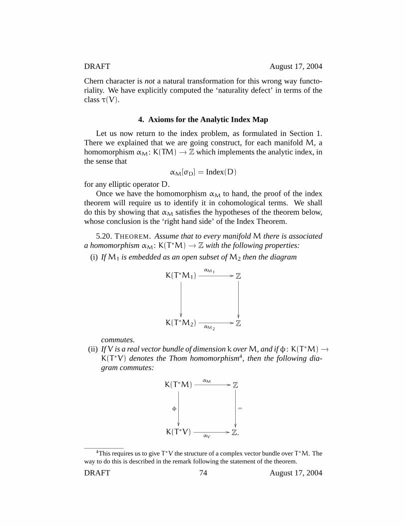
DRAFT August 17, 2004
Chern character isnot a natural transformation for this wrong way functo-riality. We have explicitly computed the ‘naturality defect’ in terms of theclassτ(V).
4. Axioms for the Analytic Index Map
Let us now return to the index problem, as formulated in Section 1.There we explained that we are going construct, for each manifoldM, ahomomorphismαM : K(TM) → Z which implements the analytic index, inthe sense that
αM[σD] = Index(D)
for any elliptic operatorD.Once we have the homomorphismαM to hand, the proof of the index
theorem will require us to identify it in cohomological terms. We shalldo this by showing thatαM satisfies the hypotheses of the theorem below,whose conclusion is the ‘right hand side’ of the Index Theorem.
5.20. THEOREM. Assume that to every manifoldM there is associateda homomorphismαM : K(T ∗M) → Z with the following properties:
(i) If M1 is embedded as an open subset ofM2 then the diagram
K(T ∗M1)αM1 //
Z
K(T ∗M2) αM2
// Z
commutes.(ii) If V is a real vector bundle of dimensionk overM, and ifφ : K(T ∗M) →
K(T ∗V) denotes the Thom homomorphism4, then the following dia-gram commutes:
K(T ∗M)αM //
φ
Z
=
K(T ∗V)
αV
// Z.
4This requires us to giveT∗V the structure of a complex vector bundle overT∗M. Theway to do this is described in the remark following the statement of the theorem.
DRAFT 74 August 17, 2004

DRAFT August 17, 2004
(iii) If b ∈ K(T ∗Rn) is the Bott element5, thenαRn(b) = 1.
Then
(3) αM(x) = (−1)dim(M)
∫T∗M
Todd(TM⊗ C) · ch(x),
for everyM and everyx ∈ K(T ∗M).
5.21. REMARK . We need to make various conventions about complexstructures, orientations, and so on. We need to know thatT ∗V is naturally acomplexvector bundle overT ∗M. By choosing Euclidean metrics one canidentify TM andT ∗M as real vector bundles, and similarly one can identifyTV andT ∗V . Thus it is enough to exhibitTV as a complex vector bundleoverTM. But in fact
TV ∼= π∗(V ⊕ V), (whereπ : TM → M),
and we can identifyV ⊕ V = V ⊗ C.The final formula 3 requires that we orientT ∗M. This we do as
follows. Choose local coordinatesx1, . . . , xn onM and correspondingcoordinatesξ1, . . . , , ξn in the fibers ofT ∗M. Then we deem that the listx1, ξ1, . . . , xn, ξn is an oriented local coordinate system onT ∗M.
5.22. REMARK . Note that axioms (i) and (ii) above simply say thatα isnatural with respect to the two sorts of ‘wrong way maps’ that we identifiedin Remark 5.19.
PROOF OFTHEOREM 5.20. We are going to approach this proof byeasy stages, so consider first the case of Euclidean spaceRn, and theassociated homomorphism
αRn : K(T ∗Rn) → K(pt).
According to the normalization axiom (iii),αRn(b) = 1 ∈ K(pt). On theother hand, on the right-hand side of formula 3 the Todd genus is equal to 1(because the tangent bundle toRn is trivial) and so we are required simplyto integrate the Chern character of the Bott class. By remark 5.17, the resultis (−1)n. So formula 3 is correct onb ∈ K(T ∗Rn). But, according tothe Bott Periodicity Theorem 5.11 (which is here used in a crucial way),the elementb generates all ofK(T ∗Rn). Thus the formula is correct onevery element ofK(T ∗Rn). Now using axiom (i), it is easy to show that theformula is correct on any open subsetU of Rn. (Of course, for such aUthe tangent bundle is still trivial, so that the Todd genus is again 1 and theformula readsαU(x) = (−1)n
∫T∗U
ch(x).)
5We considerT∗Rn as a complex vector space via the formulai · (x, ξ) = (−ξ, x),whereX ∈ Rn andξ ∈ T∗xRn ∼= Rn
DRAFT 75 August 17, 2004
DRAFT August 17, 2004
The Tubular Neighborhood Theorem of differential topology tells usthat, given any manifoldM, there is a real vector bundleV of somedimensionk overM such that the total space ofV is diffeomorphic to anopen subset ofRn. Thus the formula 3 holds forV and we will finish theproof by deducing the formula forM from that forV , using of course theaxiom (ii) which refers to the Thom isomorphism.
By that axiom we obtain, forx ∈ K(T ∗M),
αM(x) = αV(φ(x)) = (−1)n+k
∫T∗V
ch(φ(x)),
using formula 3 forV . On the right hand side of this equation applyProposition 5.14 to get
αM(x) = (−1)n+k
∫T∗M
τ(V ⊗ C) ch(x),
whereτ is the genus corresponding to the power series(1 − ex)/x. (Weare using here the fact thatT ∗V , as a complex vector bundle overT ∗M, isisomorphic toπ∗(V ⊗ C).) To finish the proof, note that the direct sumV ⊕ TM is isomorphic to a trivial bundle (of dimensionn+ k). Thus
τ(V ⊗ C) = (−1)k/Todd(V ⊗ C) = (−1)k Todd(TM⊗ C)
using Exercise 5.18 and the fact that the complexification of a real vectorbundle is isomorphic to its conjugate. Substituting this into the previouslydisplayed equation we obtain the result.
5. The Signature Operator
In this section we are going to outline an important application of theHirzebruch signature theorem to the construction of anexotic sphere. Thisis due to Milnor (1957) and it highlighted the importance of playing offagainst one another two sources of ‘integrality’ in the signature theorem: thefact the the signature (or more generally the index of an elliptic operator) isan integer, and the fact that the Pontrjagin classes are integral cohomologyclasses. It is interesting that innoncommutative geometry only the firstsource of integrality (index theory) is available to us.
The geometric input that is needed is a construction of manifolds withprescribed intersection form (remember that theintersection formis theform defined by the cup-product on the middle-dimensional cohomology).We will be considering manifoldsW with boundary, whose boundary istopologically a sphere; if you don’t want to work out a general theory ofintersection forms for manifolds with boundary, justdefinethe intersectionform of such a manifold to be the intersection form of the topologicalmanifold obtained by capping off the boundary with a disk.
DRAFT 76 August 17, 2004

DRAFT August 17, 2004
A quadratic form over the integers is said to beevenif it can be repre-sented by a matrix all of whose diagonal entries are even, andunimodularif its determinant is± 1. Milnor gave an explicit construction, sometimescalled ‘plumbing’, which will produce a smoothW with prescribed evenintersection form; unimodularity implies that the boundary is topologicallya sphere. In particular
5.23. THEOREM (Milnor Plumbing). There is a smooth 8-dimensionalmanifoldW with boundary, such that
• Σ = ∂W is homeomorphic toS7;• W is parallelizable (its tangent bundle is trivial);• The intersection form ofW is theE8 matrix,
E8 =
2 0 − 1 0 0 0 0 0
0 2 0 − 1 0 0 0 0
− 1 0 2 − 1 0 0 0 0
0 − 1 − 1 2 − 1 0 0 0
0 0 0 − 1 2 − 1 0 0
0 0 0 0 − 1 2 − 1 0
0 0 0 0 0 − 1 2 − 10 0 0 0 0 0 − 1 2
TheE8 form is even, unimodular, andpositive definite: it is the ‘small-
est’ integral quadratic form with these properties.We are going to show thatΣ is not diffeomorphicto S7: it is an ‘exotic
sphere’. For, suppose that it were. Then we could form a smooth, closed8-manifoldM by attaching an 8-disk to∂W. Applying the Hirzebruchsignature theorem we get
Sign(M) = 〈L(TM), [M]〉;that is
8 =1
45(7p2 + p21)
where the Pontrjagin classesp1 andp2 are (implicitly) evaluated on thefundamental class ofM. Recall, however, that the tangent bundle ofW
is trivial. ThusTM is obtained by ‘clutching’ two trivial bundles over the7-sphere, and in such circumstances it is easy to see that all but the highestPontrjagin classes must vanish. We conclude thatp1 = 0 so
p2 =56
45
which contradicts the integrality of the Pontrjagin classes.
DRAFT 77 August 17, 2004

CHAPTER 6
The Dirac Operator
Before commencing the proof of the index theorem are going to workout the especially important example of theDirac operator. Atiyah andSinger were developed (or rediscovered) the Dirac operator to serve as acounterpart in the realm of real manifolds, of the Dolbeault operator incomplex manifold theory. Accordingly, we shall take a quick look at theDobeault operator first.
1. The Dolbeault Operator
In this section we shall assume that the reader has some very basicfamiliarity with complex manifold theory. See for instance []. LetM bea compactcomplex hermitian manifoldof complex dimensionk, and hencereal dimension2k (see for example [] for an introductory account). Thespace of ordinary1-forms onM (with complex coefficients) decomposesas a direct sum
∧1M = ∧0,1M⊕∧1,0M,
with the first summand generated locally by thedzi and the second by thedzj. The de Rham differential decomposes as a direct sum
d = ∂+ ∂ : Ω0(M) → ∧0,1M⊕∧1,0M.
There is a corresponding decomposition of differential forms and the deRham operator in higher degrees, so that for example
∧rM = ⊕p+q=r ∧p,qM.
The space∧0,q M is isomorphic to the space of smooth sections of thebundle ∧q TM, where here we regardTM as a complex vector bundle todefine the exterior power.
We can consider theDolbeault complex
Ω0(M)∂ // Ω0,1(M)
∂ // · · · ∂ // Ω0,k(M)
and associatedDolbeault operatorD = ∂+ ∂∗. This is an elliptic operator,
and in fact its symbol is a familiar object. Namely, after we use thehermitian metric to identifyT ∗M and TM as smooth manifolds (not as
79
DRAFT August 17, 2004
complex vector bundles) the symbol ofD can be identified with the Thomelement for the pullback of∧∗ TM to TM:
σD = b : π∗ ∧∗ TM → π∗ ∧∗ TM.
Because of this we can readily compute the contribution of its Chern char-acter to the index formula. We get
Index(D) =
∫T∗M
τ(TM)uT∗M Todd(TCM)
where the overall sign(−1)n has been dropped sincen is even. NowM,being a complex manifold, is naturally oriented, and if we orientT ∗M usinglocal coordinatesx1, . . . , xn, ξ1, . . . , ξn, wherex1, . . . , xn are oriented lo-cal coordinates onM, then we can compute the integral by first integratingalong the fibers ofT ∗M. We get∫
T∗M
τ(TM)uT∗M Todd(TCM) =
∫M
τ(TM) Todd(TCM).
However this new orientation onT ∗M differs from the orientation providedin Remark 5.21 by the sign(−1)
n(n−1)2 . Bearing this in mind, and since
(−1)n(n−1)
2 = (−1)k, we obtain the index formula
Index(D) = (−1)k∫M
τ(TM) Todd(TCM).
Finally, the bundleTCM is isomorphic, as a complex vector bundle, toTM⊕ TM (the overline denotes the complex conjugate bundle). As a result
Todd(TCM) = Todd(TM) · Todd(TM).
Now using exercise 5.18 again, we obtain theHirzebruch Riemann-Rochformula
Index(D) =
∫M
Todd(TM).
6.1. EXERCISE. (For those who know some complex manifold theory.)Check Hirzebruch’s formula forCP1. For extra credit, do the same forCPn(in all cases you should get1 = 1).
Let M be an oriented, Riemannian manifold. The signature operatorD onM was discussed in Lecture 1. Its square is the Laplace operator ondifferential forms. If we square its symbolσ we find the key property that
σ(x, ξ)2 = ‖ξ‖2 · I,
which we used to infer thatD is elliptic.
DRAFT 80 August 17, 2004

DRAFT August 17, 2004
Formulas of this type are common throughoutK-theory and index the-ory. For example we encountered essentially the same identity in our treat-ment of the Bott element and the Thom homomorphism. We saw in Exam-ple?? that the signature operator is not the only operator whose symbol hasthis feature that it is the square root of the function‖ξ‖2 · I. In this lecturewe shall define and study the Dirac operator, which is in many respects themost important and most basic example of such an operator.
2. Clifford Symbols
6.2. DEFINITION. Let V be a euclidean vector bundle over some baseX. A (complex)Clifford symbolassociated toV consists of the following:
(i) A Z/2-graded hermitian vector bundleS overX;(ii) An R-linear vector bundle map
c : V → End(S)
whose values are all odd-graded, self-adjoint endomorphisms ofS,which satisfies the relation
c(v)2 = ‖v‖2 · I,
for all v ∈ V .
6.3. REMARK . We can also define areal Clifford symbol in the sameway, by replacing the hermitian vector bundleS with a euclidean vectorbundle. We will take a quick look at these at the end of the lecture.
We shall be most interested in the case whereV is the cotangent bundleof a Riemannian manifold, in which case we can view a Clifford symbol asthe symbol of some elliptic operator onM. Notice that a Clifford symboldefines an elliptic endomorphism of the pullbackπ∗S of S overV , and thusdefines aK-theory class[c] ∈ K(V) by the difference bundle constructionof 3.25.
6.4. EXAMPLE . Suppose thatV is a complex hermitian bundle, and letS = ∧∗V . The formula
b(v)w = v∧w+ v w
(which we used to define the Thom class inK-theory) is an example of aClifford symbol.
To put it another way, Clifford symbols generalize the Thom elementconstruction that we introduced in the previous lecture. The name “Cliffordsymbol” is borrowed from the following construction in algebra:
DRAFT 81 August 17, 2004

DRAFT August 17, 2004
6.5. DEFINITION. LetV be a finite-dimensional euclidean vector space.Thecomplex Clifford algebraC(V) is the complex, associative algebra withunit which is characterized up to canonical isomorphism by the followingproperties:
(i) There is a real linear mapc : V → C(V), such thatc(v2) = ‖v‖2I, forall v ∈ V .
(ii) If A is any associative algebra with unit equipped with a real linearmapcA : V → A such thatc(v2) = ‖v‖2I, for all v ∈ V , then there isa unique algebra homomorphismC(V) → A such that the diagram
Vc
zzzz
zzzz cA
>>>
>>>>
>
C(V) // A
commutes
It is easy to check that ifv1, . . . , vk is a basis forV then the set ofproductsc(vi1) · · · c(vip), wherei1 < · · · < ip, is a linear basis forC(V).ThusC(V) is a finite-dimensional algebra, with
dim(C(V)) = 2dim(V).
The algebraC(V) isZ/2-graded by assigning the monomialc(vi1) · · · c(vip)even or odd degree, according asp is even or odd. A little less obvious isthe following important fact:
6.6. PROPOSITION. If V has even dimension2k, thenC(V) is isomor-phic to the algebra of2k × 2k complex matrices.
PROOF (SKETCH/EXERCISE). We shall construct an explicit represen-tation fromC(V) into the matrix algebra, and proving using a linear basisfor C(V) that it is injective (and hence surjective too, by dimension count-ing). To do this, observe that Ifv1, . . . , v2k is an orthonormal basis forV ,and if matricesE1, . . . , E2k are given such that
E2i = I and EiEj + EjEi = 0 when i 6= j
then the formula
c(a1v1 + · · ·+ a2kv2k) = a1E1 + · · ·+ anEndefines a representation of the Clifford algebra. For example, ifk = 1, thenwe can define
c(v1) =
(0 1
1 0
)and c(v2) =
(0 i
− i 0
).
We leave it to the reader to work out suitable formulas for generalk. (Fork = 2 you will find them in Dirac’s book on quantum mechanics.)
DRAFT 82 August 17, 2004

DRAFT August 17, 2004
6.7. EXERCISE. We can make this argument a little slicker if we areprepared to use the notion ofgraded tensor product, which we alreadydiscussed in Lecture 3 in connection withC∗-algebras. For it is not hardto see from the universal property thatC(V⊕W) ∼= C(V)⊗C(W). On theother hand, we have explicitly computed above that ifV is 2-dimensional,C(V) is isomorphic to the graded algebra of endomorphisms of the gradedvector spaceH = C⊕ C. Therefore we obtain
C(C2k) = C(C2)b⊗k = End(Hb⊗k) = End(C2k−1 ⊕ C2k−1) = M2k(C).
This argument gives us the grading and∗-algebra structure too (see the nextremark).
6.8. EXERCISE. Following up on the previous exercise, suppose thatc1 andc2 are Clifford symbols for bundlesV1 andV2, acting onS1 andS2respectively. Show that theirsharp product
c1]c2 = c1⊗1+ 1⊗c2
is a Clifford symbol forV1 ⊕ V2 acting onS1⊗S2. For extra credit, showthat the associatedK-theory classes satisfy
[c1]c2] = [c1] · [c2],
and thus that ch(c1]c2) = ch(c1) ch(c2).
6.9. REMARK . It is easy to check that ifV is any euclidean vector space,then there is a unique∗-algebra structure onC(V) for whichc(v)∗ = c(v),for all v. If dim(V) = 2k thenC(V) is ∗-isomorphic to the matrix algebraM2k(C), with its usual∗-algebra structure of conjugate transpose. Inaddition, we can find a grading preserving∗-isomorphism, whereM2k(C)is graded as an algebra of block2 × 2 matrices. We shall use theserefinements of Proposition 6.6 at one or two points below.
6.10. REMARK . Proposition 6.6 is not true for odd-dimensionalV , andthis is the reason that we shall restrict to even-dimensionalV for the rest ofthis lecture. There are odd-dimensional counterparts to the proposition andto most of what follows, but they are rather more complicated and will notbe discussed in these notes.
To return to our notion of Clifford symbol, from the vector bundleV wecan form the bundleC(V) of Clifford algebras, and it is clear that a Cliffordsymbol is the same thing as a homomorphism of bundles fromC(V) intoEnd(S), which is fiberwise a homomorphism ofZ/2-graded algebras.
DRAFT 83 August 17, 2004

DRAFT August 17, 2004
3. Dirac Symbols
6.11. DEFINITION. Let V be a euclidean vector bundle ofevendi-mensionn = 2k. A Dirac symbolassociated toV is a Clifford symbolc : V → End(S) such that the vector spacesSx have (complex) dimension2k.
The condition on dim(S) specifies the minimal possible dimension ofS, in view of the following result:
6.12. LEMMA . If c : V → End(S) is a Clifford symbol associated to aeuclidean vector bundle, and ifdim(V) = 2k, then the fiber dimension ofS is a multiple of2k.
PROOF. The fibers ofS are representation spaces of the Clifford algebraof 2k-dimensional euclidean vector spaces. Since the Clifford algebras areall isomorphic to the matrix algebraM2k(C), all such representations aremultiples of the standard representation, of dimension2k.
Why the interest in Dirac symbols? They play the same role inK-theorythat orientations of vector bundles play in cohomology theory. It can beshown that ifV is an even-dimensional euclidean vector bundle overX, andif c : V → End(S) is a Dirac symbol, then theK-theory classc ∈ K(V)freely generatesK(V) as a module overK(M). Thus the existence of aDirac symbol is a sufficient (and as it happens necessary) condition for theformulation of a Thom isomorphism theorem inK-theory.
Not every vector bundleV admits a Dirac symbol. At the very least,Vmust be orientable:
6.13. LEMMA . If V is even-dimensional and ifσ : V → End(S) is aDirac symbol thenV is oriented by the following requirement: a localorthonormal framev1, . . . , v2k is oriented if and only if the operator
γ = ikσ(v1) · · ·σ(v2k)
is the grading operator of the bundleS (in other wordsγ is + I on the evenpart ofS and − I on the odd part).
PROOF. The elementγ has the following properties:γ = γ∗; γ2 = 1;andγ anticommutes with everyc(v). Using the explicit basis forC(V)given earlier, it is not hard to check that there are precisely two elements inany Clifford algebra with these properties, which differ from one anotherby a sign only. Under the isomorphism of bundlesc : C(V) → End(S), oneof ± γ corresponds to the grading operator and one to its negative (sincethe grading operator and its negative have the same properties). We cantherefore specify a family of consistent orientations in the fibers ofV byrequiring that in every fiber,γ corresponds to the grading operator.
DRAFT 84 August 17, 2004
DRAFT August 17, 2004
6.14. REMARK . From now on we shall assume thatV is oriented andthat the orientation is compatible with the grading onS, as specified in thelemma.
Not every orientable vector bundle admits a Dirac symbol; for instance,the tangent bundle to the orientable manifoldSU(3)/SO(3) does not1.There is however a simple sufficient condition: ifV is (the underlying realvector bundle of) a complex hermitian bundle, it admits a Dirac symbol,namely the one given in Example 6.4.
We shall say a bit more later about conditions necessary to guaranteethe existence of Dirac symbols. But let us note now that Dirac symbols arenot necessarily unique. Indeed, ifc : V → End(S) is a Dirac symbol and ifL is a complex line bundle, then the object
c⊗ idL
: V → End(S⊗ L)
is also a Dirac symbol.
6.15. LEMMA . Let c1 : V → End(S1) and c2 : V → End(S2) betwo Dirac symbols associated to an even-dimensional, oriented euclideanvector bundleV . The formula
L = HomV
(S1, S2)
defines a line bundle, for whichc2 : V → End(S2) is isomorphic to thetensor product
c1 ⊗ idL
: V → End(S1 ⊗ L).
PROOF. By HomV(S1, S2) we mean the vector bundle whose fibers arethe complex linear maps from the fibers ofS1 to the fibers ofS2 whichare of evenZ/2-grading degree and which commute with the action of thefibers ofV . Neglecting the orientation condition, the fact that the actionof the fiberVx corresponds to an irreducible representation of the CliffordalgebraC(Vx) proves that the fibers of HomV(S1, S2) are one-dimensionalvector spaces (this is Schur’s Lemma in representation theory). The factthat the elements of HomV(S1, S2) are grading-preserving follows from ourorientation assumption. The isomorphism in the statement of the lemmacomes from the canonical evaluation map
S1 ⊗ HomV
(S1, S2) → S2,
so the proof of the lemma is complete.
1The proof of this result is out of reach using the techniques we have developed so far.
DRAFT 85 August 17, 2004

DRAFT August 17, 2004
4. Chern Character of Dirac Symbols
If c : V → End(S) is a Dirac symbol then so is the adjoint mapc∗ : V → End(S∗). The construction in Lemma 6.15 therefore allows usto associate to a single Dirac symbolc : V → End(S) a line bundleEc bythe formula
Ec = HomV
(S∗, S).
Note that by the canonical evaluation map given in the proof of Lemma 6.15,Ec ⊗ S∗ ∼= S.
6.16. EXERCISE. Show that ifL is an auxiliary line bundle, and ifσL = c⊗ idL, thenEcL
∼= Ec ⊗ L⊗ L.
6.17. EXERCISE. Show that ifV is ann-dimensional complex vectorbundle and ifb : V → End(∧∗V) is the Thom element, viewed as a Diracsymbol, thenEb = ∧nV . (This is a little tricky.)
Our aim is to prove the following result:
6.18. PROPOSITION. Let V be an euclidean vector bundle of rank2kover a compact manifoldM. If c : V → End(S) is a Dirac symbol, then
ch(c) = (−1)k√
ch(Ec)√τ(V ⊗ C)uV ∈ H∗(W)
whereuV ∈ H∗(V) is the cohomology Thom class ofV and τ is themultiplicative characteristic class of complex vector bundles associated tothe power series(1− ex)/x.
The formula requires a little bit of interpretation. Note that the classesτ(V⊗C) and ch(Ec) both are elements of the graded ringH∗(M) and havedegree zero term equal to 1. Square roots of such elements (in any gradedring) may be defined by the usual binomial formula
(1+ x)12 = 1+
1
2x−
1
8x2 + · · · .
In fact, sinceEc is a line bundle, its Chern character is simplyex, wherex = c1(Ec) is the Chern class ofEc. The square root of this Chern characteris of course justex/2.
PROOF OF THEPROPOSITION(SKETCH). Consider the euclidean vec-tor bundleV ⊕ V . There aretwo natural ways to construct a Dirac symbolon this bundle:
(i) We may form the product symbol2 c]c of two copies of the given Diracsymbolc;
2See Exercise 6.8.
DRAFT 86 August 17, 2004

DRAFT August 17, 2004
(ii) Ignoring the given symbolc entirely, we may considerV ⊕ V as theunderlying real vector bundle of the complex vector bundleV ⊗ C,and then form the associated Dirac symbol according to example 6.4.
Call these Dirac symbolsc1, c2, acting onS1, S2 respectively. According toLemma 6.15 there is a line bundleL such thatS2 = S1⊗L andc2 = c1⊗1.What is this line bundle? We shall see that it is simplyE∗c, the dual of thecanonical line bundle associated to the original Dirac symbol.
Once we have this information we may proceed as follows. Letc ∈K(V) be theK-theory class of the Dirac symbolc : V → End(S), and leta(c) be the cohomology class determined by the formula
ch(c) = a(V)uV ∈ H∗(V).
By following the same line of reasoning that we used in the last lecture,one can show thata(c) is multiplicative, in the sense thata(c ′]c ′′) =a(c ′) · a(c ′′). In particular we have
ch(c1) = a(c)2 · uV⊗C ∈ H∗(V ⊗ C).
On the other hand,c2 is just theK-theory Thom class associated to thecomplex vector bundleV ⊗ C, so according to Theorem 5.16 from theprevious lecture,
ch(c2) = τ(V ⊗ C)uV⊗C.
UsingS2 = S1 ⊗ E∗c, we obtain
τ(V ⊗ C) = a(c)2 ch(E∗c),
and so
a(c) = ±√
ch(Ec)√τ(V ⊗ C).
This is what we want, except that we have to check that the sign is correct.To do this we just need to work out the degree zero part ofa(c) in H0(M),and to do this we can restrict the bundleV to a single point inM. Here,over a single point, we can giveV a complex structure, and since all linebundles over a point are trivial, the restriction of the Dirac symbol to ourpoint is isomorphic to the Bott element forV over this point (considered asa complex vector space). The computations in the previous lecture now tellus that the correct sign is(−1)k (wherek is the complex dimension of therestrictedV).
It remains to explain why it is thatS2 = S1 ⊗ E∗c. Begin by consideringC(V), the bundle of Clifford algebras overV . Like any algebra, theClifford algebra is of course abimoduleover itself, using the actions ofleft and right multiplication. These actions commute: but we can make
DRAFT 87 August 17, 2004
DRAFT August 17, 2004
them anticommute instead by introducing a small twist from the gradingautomorphismα:
L(u) · x = ux, R(v) · x = α(x)v.
Now L andR define anticommuting Clifford symbols forV , so the pair(L, R) defines a Clifford symbol forV ⊕V , which (by dimension counting)must in fact be a Dirac symbol. In fact, this Dirac symbol is a familiarone: there is a canonical isomorphism of vector spaces fromC(V) to thecomplexified exterior algebra ofV , and under this isomorphism the symbol(L, R) just passes to the symbol of Example 6.4. In other words, the bundleC(V), considered as a Dirac bundle overV ⊕ V by the action(L, R), just isS2.
But we can apply our knowledge of the representation theory of theClifford algebra to understandC(V). We know that the Clifford algebrais a matrix algebra over its spin space: thus,C(V) = End(S) = S∗ ⊗ S.The effect of the ‘twist’ that we introduced above to make the left and rightactions anticommute is to replace the ordinary tensor product here by agradedtensor product, so that
S2 = S∗⊗S.
On the other hand,
S1 = S⊗S,so the desired resultS2 = S1 ⊗ E∗c now follows from the definition of thebundleEc.
6.19. DEFINITION. We shall call a (symmetric, first-order) differentialoperator aDirac operator if its symbol is a Dirac symbol associated toT ∗M.
A Dirac operator is necessarily elliptic. Our calculation of the Cherncharacter of Dirac symbols allows us to write out the index formula forDirac operators in fairly explicit terms.
6.20. THEOREM. Let D be a Dirac operator associated to a Diracsymbolσ on a compact oriented (even-dimensional) manifoldM. Then
Index(D) =
∫M
√ch(Eσ) A(TM).
where the genusA(TM) is defined in Example 4.35.
PROOF. We will deduce this from the general form of the Index Theo-rem 5.1. The idea is the same as in Example??.
DRAFT 88 August 17, 2004
DRAFT August 17, 2004
Substituting the formula of Proposition 6.18, which gives the Cherncharacter of the symbol, into the index theorem 5.1, we get
Index(D) =
∫T∗M
√ch(Eσ)
√τ(TM⊗ C) Todd(TM⊗ C)uTM.
Now the classτ is just the inverse of the Todd class (see Exercise 5.18; thereare no signs because we are in the even-dimensional case). Using this, andintegrating over the fiber, we get
Index(D) =
∫M
√ch(Eσ)
√Todd(TM⊗ C).
But according to exercise 4.36, theA genus is the square root of the Toddgenus of the complexification. This completes the proof.
6.21. EXAMPLE . If M is a complex manifold then the symbol of theDolbeault operatorD = ∂ + ∂∗ acting onS = ∧0,∗T ∗CM
∼= ∧∗TM is aDirac symbol. The line bundleLS is the dual of thecanonical line bundle:EσD
= ∧nTM (we form the highest exterior power using the complexstructure onTM).
5. Spinc-Structures and Principal Bundles
This short section is optional, and aimed at people with some familiaritywith principal bundle theory.
6.22. DEFINITION. A Spinc-structureon a Riemannian manifold is anisomorphism class of Dirac symbols associated toT ∗M.
Let us discuss in more detail the problem of determining whether or notan oriented Riemannian manifold admits a Spinc structure.
Consider the complex Clifford algebra ofR2k. It is isomorphic to matrixalgebraM2k(C):
CliffC
(R2k) ∼= M2k(C).
Let us fix such an isomorphism. The groupSO(2k) acts onR2k andtherefore on CliffC(R2k), and therefore onM2k(C) via the given, fixed,isomorphism. Since every automorphism ofM2k(C) is induced from anautomorphism ofC2
k, which is determined up to a scalar multiple of the
identity, we obtain a group homomorphism
SO(2k) → U(2k)/Z,
whereZ denotes the center of the unitary groupU(2k) (Z is isomorphic toS1 and consists of scalar multiples of the identity).
DRAFT 89 August 17, 2004
DRAFT August 17, 2004
6.23. DEFINITION. Denote by Spinc(2k) the group which fits into thepullback diagram
S1
=
// Spinc(2k) //
SO(2k)
Z // U(2k) // U(V)/Z
Observe that the group Spinc(2k) comes with canonical representationson the spacesR2k andC2k
. The mapR2k ⊗ C2k → C2kwhich is induced
from our fixed isomorphismC(R2k) ∼= M2k(C) is Spinc(2k)-equivariant.One can prove the following result.
6.24. THEOREM. An oriented Riemannian2k-manifold admits aSpinc-structure if and only if the principalS0(2k)-bundleF of oriented framesadmits a reductionF to the groupSpinc(2k). In this case, the cotangentbundleTM is given by
T ∗M = F×Spinc(2k) R2k,
and the formula
S = F×Spinc(2k) C2k
defines a hermitian bundle equipped with an actionT ∗M ⊗ S → S whichis a Dirac symbol. In this way,Spinc-structures correspond bijectively toreductions of the oriented frame bundle toSpinc(2k).
6. Spin-Structures
Let us finish by making some remarks about Dirac operators associatedto real (as opposed to complex) Dirac symbols. In the real case, we shallrestrict to manifolds of dimension8n (for the definitions we have givenhere). This is to accommodate the following result:
6.25. PROPOSITION. The real Clifford algebraR(R8m) is isomorphicto the matrix algebraM24k(R).
We define real Dirac symbols in the8k-dimensional case by puttinga minimal dimensionality requirement on the bundleS (we shall orientM compatibly with the symbol). We define a Spin-structure to be anisomorphism class of real Dirac symbols.
By following a similar reasoning to that used in the previous section onecan prove:
6.26. THEOREM. An oriented Riemannian8k-manifold admits a Spin-structure if and only if the principalS0(8k)-bundleF of oriented frames
DRAFT 90 August 17, 2004

DRAFT August 17, 2004
admits a reductionF to the groupSpin(8k). HereSpin(8k) is the doublecover ofSO(8k) which fits into the diagram
Z/2
=
// Spin(8k) //
SO(8k)
Z // SO(24k) // SO(24k)/Z
(one can show thatSpin(8n) is the simply connected double cover ofSO(8n)). In this case, the bundleS is given by
S = F×Spin(8n) R24k
,
and the action ofT ∗M on it is induced from the action ofR8n onR24k.
If the Dirac symbolc : T ∗M → End(S) is the complexification of areal Dirac symbol then the line bundleLc is trivial. In this case the indexformula reads quite simply
Index(D) =
∫M
A(M).
One of the interesting features of this formula is that in the real case,thanks to the fact that the reductionF is a covering space of the frame bundleF, there is a natural connection onF which gives rise to a natural affineconnection onS, and ultimately a canonical operator (defined in terms ofthe Riemannian geometry ofM) whose symbol is the Dirac symbol, namely
D =∑
σ(ωi)∇Xi,
where the sum is over a local frameXi and dual frameωi. This operatorhas the following important property, known as theLichnerowicz formula:
D2 = ∇∗∇+κ
4,
whereκ is the scalar curvature3 function ofM. Hence:
6.27. THEOREM. Let M be a Riemannian manifold which admits aSpin structure. If the scalar curvature ofM is everywhere positive then∫MA(M) = 0.
PROOF. If κ > 0 then by the Lichnerowicz formula the Dirac operatoris bounded below, and is therefore invertible. Hence its index is zero.
3Results of this type, known asBochner-Weitzenbock formulae, can be proved formany natural geometric operators; the point about the Dirac operator associated to a Spin-structure is that the curvature term which appears in all such formulae is of a particularlysimple sort.
DRAFT 91 August 17, 2004


CHAPTER 7
The Tangent Groupoid
In this chapter we will construct the homomorphismαM : K(T ∗M) →Z which maps the symbol class of an elliptic operatorD to the index ofD.The construction will be made using Connes’ notion oftangent groupoid.
1. Smooth Groupoids
What is non-commutative geometry? Recall that a governing idea in allsorts of ordinary geometry is that features of geometric spaces are reflectedwithin the algebras of their coordinate functions. For instance, ifX is acompact Hausdorff space then one can recoverX as the space of maximalideals of the algebraC(X) of continuous, complex-valued functions onX.Alain Connes’ non-commutative geometry is concerned with aspects of thespace–algebra correspondence which, on the algebra side, involve Hilbertspace methods, particularly the spectral theory of operators on Hilbertspace. Moreover it is a guiding principle of the theory thatnon-commutativealgebras may often arise from geometric situations, and that one should asfar as possible treat non-commutative and commutative algebras bysimilargeometric methods. One natural way to formalize this idea is by means ofthe theory of which we will develop in this chapter.
Let us begin with the following definition, which is short, but probablyopaque to anyone who has not encountered it before.
7.1. DEFINITION. A smooth groupoidis a small category in whichevery morphism is invertible, and for which the set of all morphisms andthe set of all objects are given the structure of smooth manifolds; the sourceand range maps are submersions; and the composition law and inclusion ofidentities are smooth maps.
In a more detail, a smooth groupoid consists of, to begin with, a man-ifold G, whose points constitute the morphisms (all of them, between anytwo objects) in some category; a smooth manifoldB whose points are theobjects in the category; and two mapsr, s : G → B which associate to
93

DRAFT August 17, 2004
morphisms their range and source objects and which are required to be sub-mersions1. It can be shown then that the set
G2 = (γ1, γ2) ∈ G×G : s(γ1) = r(γ2)
of composable pairs of morphisms is a smooth submanifold ofG×G. Withthis in hand we require further that the composition operation(γ1, γ2) 7→γ1 γ2 be a smooth map fromG2 to G. We also require that the mape : B → G which maps an objectx ∈ B to the identity morphism atxbe smooth. Finally, we require that every morphism in the category beinvertible; it may be shown that the mapγ 7→ γ−1 from G to itself isautomatically a diffeomorphism.
In noncommutative geometry it is customary to paint what might becalled thequotient space pictureof groupoid theory. In this view, one thinksof the morphisms inG as defining an equivalence relation on the objectspaceB: two objects are equivalent if there is a morphism between them.Two objects might be equivalent for more than one reason, and the groupoidkeeps track of this. It is customary in mathematics to form the quotientspace from an equivalence relation, but even in rather simple examples theordinary quotient space of general topology can be highly singular, and forexample not at all a manifold. The groupoid serves as a smooth stand-infor the quotient space in these situations, and using it one can study thecohomology of the quotient space, and even its geometry. These ideas aredeveloped extensively in Connes’ book [].
A second view of groupoid theory, which is better suited to our presentpurposes, is what we shall call thefamilies picture. We shall think of thegroupoid first as the family of smooth manifolds
Gx = γ ∈ G : s(γ) = x
parametrized byx ∈ B. If η is a morphism inG from x to y, then there isan associated diffeomorphism
Rη : Gy → Gx
defined byRη(γ) = γ η. We shall therefore think ofG as being asmooth family of smooth manifolds, provided with the collection of allthe intertwining diffeomorphismsRη. From this point of view, havingbeen given a groupoidG it will be very natural to consider families ofsay differential operatorsDx, one on eachGx, which are equivariant withrespect to theRη, in the obvious sense.
7.2. EXAMPLE . A Lie groupG may be viewed as a smooth groupoid.The object set is a single-element set, and the set of morphisms from this
1Recall that a smooth map between manifolds is a submersion if in suitable localcoordinates it has the form of a projection(x1, . . . , xp+q) 7→ (x1, . . . , xp).
DRAFT 94 August 17, 2004

DRAFT August 17, 2004
single element to itself isG. In the families picture, we have one manifold— the underlying smooth manifold ofG — and a family of self-maps ofthis manifold, given by the usual right-translation operators on a group. Anequivariant operator in this example is a right-translation-invariant operatoron the Lie groupG. Thus if for exampleG = Rn, then an equivariantdifferential operator is nothing but a constant coefficient operator onRn.
7.3. EXAMPLE . LetM be a smooth manifold. Thepair groupoidofMhas object spaceM, and morphism spaceG = M×M. Its structure mapsare as follows:
• Source map:s(m2,m1) = m1.• Range mapr(m2,m1) = m2.• Composition:(m3,m2) (m2,m1) = (m3,m1).• Inclusion of identities:m 7→ (m,m).
The spacesGm all identify withM, and the translation operatorsGm2→
Gm1all become the identity map under these identifications. An equivariant
family of operators in this example is nothing more than a single, butgeneral, operator on the manifoldM.
7.4. EXAMPLE . The previous two examples can be combined, after afashion, as follows. LetA be a Lie group which acts (on the left) on asmooth manifoldM. Thetransformation groupoidAnM has object spaceM and the following morphism space:
(m2, a,m1) ∈M×A×M : m2 = am1 .
Obviously the morphism space identifies with the productA × M byprojection onto the last two factors, but the above description makes thestructure maps more transparent:
• Source map:s(m2, a,m1) = m1.• Range map:r(m2, a,m1) = m2.• Composition:(m3, a2,m2) (m2, a1,m1) = (m3, a2a1,m1).• Inclusion of identities:m 7→ (m, e,m).
The inverse of(m2, a,m1) is (m1, a−1,m2). However an equivariant
family of operators is not, as one might guess, the same thing as anA-equivariant operator onM. Instead it is a family of operatorsDm onA,parametrized bym ∈ M, for which the operatorDm is equivariant for theright translation action of the isotropy subgroupAm onA.
2. Foliation Groupoids
3. The Tangent Groupoid
Let M be a smooth manifold. The tangent groupoid is a smoothgroupoid whose object space is the productM× R. In the families picture
DRAFT 95 August 17, 2004

DRAFT August 17, 2004
the tangent groupoid ofM consists of repeated copies ofM, together withthe tangent spacesTmM. These will ultimately be joined together to formthe fibers of a single smooth maps : TM → M × R. But let us begin bydescribingTM as a topological space.
7.5. DEFINITION. LetM be a smooth, open manifold. Denote byTMthe set
TM = TM×0 ∪ M×M×R×
(a disjoint union) equipped with the following topology:
(i) Any open subset ofM×M×R× is deemed to be an open set inTM.(ii) Let X be a tangent vector onM, let f : M → C be a smooth function
and letε > 0. The setUf,ε ⊆ TM defined by
Uf,ε ∩ TM×0 = (Y, 0) : |X(f) − Y(f)| < ε
and
Uf,ε ∩ M×M×R∗ =
(m2,m2, t) :
∣∣∣∣X(f) −f(m2) − f(m1)
t
∣∣∣∣ < εis an open neighbourhood ofX in TM, and the set of finite intersec-tions of such sets forms a neighborhood base atX.
7.6. REMARK . We are thinking here of a triple(m2,m1, t) as being an“approximate tangent vector” which is close to a real tangent vectorX if thedifference quotient|f(m2) − f(m1)|/t is close toX(f).
The topology onTM is easily seen to be Hausdorff. Moreover it islocally Euclidean:
7.7. LEMMA . LetM be a smooth, open manifold. IfU is an open subsetofM then the set
TU = TU×0 ∪ U×U×R×
is an open subset ofTM. Moreover ifφ : U → Rn is a diffeomorphismonto an open subset then the map
Φ : TU → Rn×Rn ×Rdefined by
Φ(X,m, 0) = (Dφm(X), φ(m), 0)
Φ(m2,m1, t) = (t−1(φ(m2) − φ(m1)), φ(m1), t)
is a homeomorphism onto an open subset.
7.8. REMARK . For clarity we are using the redundant notation(X,m),whereX ∈ TmU, to describe points ofTU. We denote byDφm : TmU →Rn the derivative ofφ atm ∈ U.
DRAFT 96 August 17, 2004

DRAFT August 17, 2004
7.9. EXERCISE. Prove the lemma.
The mapsΦ defined in the lemma determine an atlas of charts for thesmooth manifoldTM:
7.10. LEMMA . LetΦ : TU → Rn×Rn×R andΨ : TV → Rn×Rn×Rbe the maps associated to diffeomorphismsφ : U → Rn andψ : V → Rn,as in the previous lemma. The compositionΨ Φ−1 is defined on an opensubset ofRn×Rn ×R, and is a smooth map.
PROOF. The inverseΦ−1 is given by the formula
Φ−1(v2, v1, t) =
(φ−1(tv2 + v1), φ
−1(v1), t) if t 6= 0
(Dφ−1v1
(v2), φ−1(v1), 0) if t = 0.
Using the notationθ = ψ φ−1, the compositionΘ = Ψ Φ−1 is given bythe formula
Θ(w2, w1, t) =
(t−1
(θ(tw2 +w1) − θ(w1)
), θ(w1), t) if t 6= 0
(Dθw1(w2), θ(w1), 0) if t = 0.
By a version of the Taylor expansion, there is a smooth, matrix-valuedfunctionθ(h,w) such that
θ(h+w) = θ(w) + θ(h,w)h and θ(0,w) = Dθw.
So we see that
Θ(w2, w1, t) =
(θ(tw2, w1)w2, θ(w1), t
)if t 6= 0(
Dθw1(w2), θ(w1), 0
)if t = 0.
This is clearly a smooth function.
We have therefore obtained a smooth manifoldTM. It is clear that themap
s : TM → M× Rdefined bys(X,m, 0) = (m, 0) ands(m2,m1, t) = m1 is a submersion.The fibers ofs areTmM at (m, 0) andM at (m, t), whent 6= 0. Theremaining groupoid structure maps are as follows.
7.11. DEFINITION. LetM be a smooth, open manifold. Thetangentgroupoidof M is the groupoid with morphism setTM, object setM × R,and the following structure maps (in whicht 6= 0 in every formula):
• Source map:s(X,m, 0) = (m, 0) ands(m2,m1, t) = (m1, t).• Range map:r(X,m, 0) = (m, 0) andr(m2,m1, t) = (m2, t).• Composition:(X,m, 0)(Y,m, 0) = (X+Y,m, 0) and(m3,m2, t)
(m2,m1, t) = (m3,m1, t).• Inclusion of identities:(m, 0) 7→ (0,m, 0) and(x, t) 7→ (m,m, t).
DRAFT 97 August 17, 2004

DRAFT August 17, 2004
Inverses are given by the formulas(x, v)−1 = (x,−v) and (x, y, t)−1 =(y, x, t).
It is clear that if we look at the subsetTM consisting of those mor-phisms attached to a fixedt (including possiblyt = 0) then the above oper-ations provide “slice” ofTM with a groupoid structure on its own, whoseobject space isM. Whent = 0 we get the tangent bundleTM: the sourceand range maps are both the projection ontoM, and the composition lawis addition of tangent vectors. Whent 6= 0 we get the pair groupoid ofM.Thus, algebraically,TM is the union of multiple copies of the pair groupoidofM and one copy of the tangent bundle, viewed as a groupoid. Let us showthat the overall package is a smooth groupoid, first in the special case whereM = Rn:
7.12. EXAMPLE . The mapΦ : TRn → Rn× Rn×R defined by
Φ(v2, v1, 0) = (v2, v1, 0)
Φ(v2, v1, t) = (t−1(v2 − v1), v1, t) (t 6= 0)
is a diffeomorphism. Now consider the space
G = (w2, a,w1) : w1, w2 ∈ Rn × R, a ∈ Rn, w2 = a4w1 ,
where the operation4 is defined by
a4(v, t) = (v+ ta, t).
Thus the4 operation defines an action of the groupA = Rn on Rn × R,and our spaceG is the corresponding transformation groupoid. The spaceG
identifies withRn×Rn×R by droppingw2 from (w2, a,w1). Using this,we can consider the diffeormorphismΦ to be a diffeomorphismΦ : TM →G by the formulas
Φ(v2, v1, 0) = ((v1, 0), v2, (v1, 0))
Φ(v2, v1, t) =((v2, t), t
−1(v2 − v1), (v1, t))
(t 6= 0).
Using these, it is evident thatΦ is actually an isomorphism of groupoids,from which it follows that the groupoid structure onTRn is smooth.
To summarize:
7.13. PROPOSITION. Denote byG = Rn n Rn,1 the transformationgroupoid associated to the action ofRn on the spaceRn,1 = Rn×R givenby the formula
a4(v, t) = (v+ ta, t) ( a ∈ Rn and(v, t) ∈ Rn,1).DRAFT 98 August 17, 2004
DRAFT August 17, 2004
The mapΨ : TRn → G which is given by the formulas
Φ(v2, v1, 0) = ((v1, 0), v2, (v1, 0))
Φ(v2, v1, t) =((v2, t), t
−1(v2 − v1), (v1, t))
(t 6= 0).
is an isomorphism of smooth groupoids.
7.14. REMARK . The groupoidTRn only depends on the smooth struc-ture of Rn, whereas, superficially at least, the groupoidG = Rn n Rn,1depends very much on the vector space structure ofRn. The propositionshows that this dependence is an illusion.
7.15. PROPOSITION. The structure maps are all smooth, and the sourceand range maps are submersions. ThusTM is a smooth groupoid.
PROOF. Since smoothness is a local property, we can check this in acoordinate neighbourhoodU. Since the construction ofTU is coordinate-independent we can assume thatU = Rn, and thereby reduce to theexample just considered.
4. Groupoid Algebras
We are going to associate to a smooth groupoid a convolutionC∗-algebra, generalizing the reduced groupC∗-algebra of a Lie group.
7.16. DEFINITION. A right Haar systemon a smooth groupoidG is asystem of smooth measures, one on each of the manifolds
Gx = γ ∈ G : s(γ) = x ,
with the properties that:
(i) If f is a smooth, compactly supported function onG then∫Gxf(γ)dµx(γ)
is a smooth function ofx.(ii) If η is a morphism fromx to y then∫
Gx
f(γ)dµx(γ) =
∫Gy
f(γ η)dµy(γ).
7.17. PROPOSITION. Every smooth groupoid admits a right Haar sys-tem.
The proposition can be proved by adapting the standard constructionof Haar measures on Lie groups: pick a1-density (basically a top degreedifferential form) onGx at the point idx and do so in a way which variessmoothly withx. Then right-translate the densities aroundG to define a1-density at every point with the required properties.
DRAFT 99 August 17, 2004

DRAFT August 17, 2004
7.18. DEFINITION. LetG be a smooth groupoid with right Haar system.Define a convolution multiplication and adjoint on the spaceC∞
c (G) ofsmooth, compactly supported complex functions on the morphism spaceof G using the formulas
f1 ? f2(γ) =
∫Gs(γ)
f1(γ η−1)f2(η)dµs(γ)(η).
and
f∗(γ) = f(γ−1).
7.19. PROPOSITION. Let G be a smooth groupoid with right Haarsystem. With the above operations,C∞
c (G) is an associative∗-algebra.
7.20. DEFINITION. LetG be a smooth groupoid with right Haar system.Define representations
λx : C∞c (G) → B(L2(Gx))
by the formulas
λx(f)h(γ) = f ? h(γ) =
∫Gs(γ)
f(γ η−1)h(η)dµs(γ)(η).
The reduced groupoidC∗-algebraof G, denotedC∗λ(G), is the completion
of C∞c (G) in the norm
‖f‖ = supx‖λx(f)‖B(L2(Gx)).
7.21. EXAMPLE . If G = M×M (the pair groupoid), then in any Haarsystem all the measuresµm onGm = M × m ∼= M are equal to oneanother and conversely any smooth measureµ determines a Haar system.The convolution multiplication and adjoint are
f1 ? f2(m2,m1) =
∫M
f1(m2,m)f2(m,m1)dµ(m).
and
f∗(m2,m1) = f(m1,m2).
The groupoidC∗-algebraC∗λ(G) is theC∗-algebra of compact operators on
L2(M).
7.22. EXAMPLE . If G = TM (the tangent bundle) then a Haar system isa smoothly varying system of translation-invariant measures on the vectorspacesTmM. Since a translation-invariant measure onTmM is the samething as a point in∧n T ∗mM, we see that a smooth Haar system onTM
DRAFT 100 August 17, 2004
DRAFT August 17, 2004
is determined by a smooth measure onM. The convolution multiplicationand adjoint in the groupoid algebra are
f1 ? f2(X,m) =
∫TmM
f1(X− Y,m)f2(Y,m)dµ(Y).
andf∗(X,m) = f(−X,m).
The groupoidC∗-algebra is therefore, so to speak, a bundle ofC∗-algebrasoverM, whose fiber atm ∈M is the groupC∗-algebra ofTmM. Considerthe tangent bundleTM. But to get a clearer picture of it, let us invoke someFourier theory, as follows. The Fourier transform
h(η) =
∫TmM
e−iη(X)h(X)dX (η ∈ T ∗mM)
determines an isometric isomorphismL2(TmM) ∼= L2(T ∗mM) (for a suit-able Haar measure onT ∗mM). If f ∈ Cc(TM) then let
f(η,m) =
∫TmM
e−iη(Y)f(Y,m)dy.
The functionf is continuous and vanishes at infinity on the cotangent bundleT ∗M. Sincef ? h = f · h (pointwise multiplication) we obtain, with a littlemore work, a Fourier isomorphism
C∗λ(TM) ∼= C0(T
∗M).
5. The C*-Algebra of the Tangent Groupoid
Let M be a smooth manifold without boundary. To define a smoothHaar system on the tangent groupoidTM, first fix a smooth measureµonM. As we noted above,µ determines a family of translation invariantmeasuresµm on the vector spacesTmM. We define smooth measures onthe fibersTM(m,t) of the source map by the formulas
µm,0 = µm onTM(m,0)∼= TxM
andµ(m, t) = t−nµ onTM(m,t)
∼= M.
7.23. LEMMA . The above formulas define a smooth right Haar systemonTM.
PROOF. The measures certainly constitute a translation-invariant sys-tem (compare Examples 7.21 and 7.22 above). To prove they are smoothwe shall make use of the diffeomorphismsΦ introduced in the previoussection, or rather their inversesΘ = Φ−1 : Rn × Rn × R → TU. Let us
DRAFT 101 August 17, 2004
DRAFT August 17, 2004
choose coordinates onU ⊆ M so that the diffeomorphismφ : U → Rnfrom whichΦ is defined is the identity in these local coordinates. Then
Θ(X,m, 0) = (X,m, 0) andΘ(m2,m1, t) = (m1+tm2,m1, t), if t 6= 0.
If we restrict to one of the fibers of the source map then we obtain the maps
Θm1,0(X) = X ∈ Tv1U
andΘm1,t(v2) = v1 + tv2 ∈ U.
The derivatives of these maps (expressed as matrices, using our chosencoordinates) areI in the first case andtI in the second. Now, to transferthe measures from the fibers ofTU to the fibers (under projection onto thelast two factors) ofRn × Rn × R, we must multiply by the determinantof these derivative matrices. That is, ifΘ : A → B is a diffeomorphismbetween open sets inRk, and ifµ(b) = m(b)db is a smooth measure onB, then∫B
f(b)dµ(b) =
∫B
f(b)m(b)db =
∫A
f(Θ(a))m(Θ(a)) det(DΘa)da.
In our case we see that the factort−n in the definition ofµm,t cancels withdet(DΘ) = tn, and we obtain smoothly varying measures, as required.
TheC∗-algebra of the tangent groupoid comes equipped with a familyof restriction∗-homomorphisms
ε0 : C∗λ(TM) → C0(T
∗M)
and, fort 6= 0,εt : C
∗λ(TM) → K(L2(M)).
On the subalgebraC∞c (TM) these are defined by restricting functions on
Tm to the “slice” of TM over t, which is either the tangent bundleTM(whent = 0) or the pair groupoidM×M (whent 6= 0). Strictly speaking,whent 6= 0 the restriction∗-homomorphism lands in the compact operatorson the Hilbert spaceL2(M,S) associated to the measureµ scaled byt−n.But this Hilbert space is obviously unitarily equivalent to the Hilbert spaceassociated toµ itself: just multiply byt
n2 . The restriction homomorphisms
will be put to good use in the next section to finally construct the indexhomomorphism inK-theory.
6. The Index Homomorphism
The∗-homomorphismε0 : C∗λ(TM) → C0(T
∗M) is surjective. Let usfix a set-theoretic sectionσ : C0(T
∗M) → C∗λ(T
∗M). The mapσ need haveno other property than thatε0 σ = id, although it is for example possibleto chooseσ to be linear and continuous.
DRAFT 102 August 17, 2004
DRAFT August 17, 2004
7.24. LEMMA . The family of mapsαt : C0(T ∗M) → K(L2(M)) definedby the formula
αt(h) = εt−1(σ(h)) (t ∈ [1,∞), h ∈ C0(T ∗M)),
is an asymptotic morphism.
PROOF. Exercise.
7.25. DEFINITION. The index homomorphismα : K(T ∗M) → K(pt) istheK-theory map induced from the above asymptotic morphismα : C0(T
∗M) →K(L2(M)).
7. Elliptic Operators and the Tangent Groupoid
LetM be a smooth manifold and letD be a partial differential operatoron M. To keep within the framework developed in Chapter 2, let usassume right away thatD has order1, although this assumption will onlybe essential later in the section.
Recall that we had associated toD a family of “model operators”Dm,which are translation-invariant partial differential operators on the tangentspacesTmM. They were obtained by freezing the coefficients ofD atm.Thus ifD =
∑ajX
j + b, where theaj andb are smooth functions onMand theXj are vector fields, thenDm =
∑aj(m)Xjm, where we view the
tangent vectorXjm as a directional derivative onTmM.Let us now associate toD a family of partial differential operators on
the fibers of the source map for the tangent groupoid. To define the family,we shall identify the fibers associated tot = 0with the tangent spacesTmMand the fibers associated tot 6= 0 withM itself, in the obvious way. Havingdone so, we define
Dm,0 = Dm onTmM
Dm,t = tD onM.
7.26. PROPOSITION. The operatorsDm,t, for m ∈ M and t ∈ R,constitute a smoothly varying family of operators on the fibers of the sourcemaps : TM → M× R.
7.27. REMARK . By “smoothly varying” we mean that if the family isapplied fiber-wise to a smooth function onTM then the result is anothersmooth function onTM.
PROOF. Let us verify this locally by transferring the problem toRn ×Rn × R using our standard diffeomorphismΦ : TU → Rn × Rn × R. As
DRAFT 103 August 17, 2004

DRAFT August 17, 2004
in the last section, let us choose coordinates onU so thatΦ has the simpleform
Φ(X,m, 0) = (X,m, 0) and Φ(m2,m1, t) = (t−1(m2 −m1),m1, t).
Write D =∑aj∂j + b. Then underΦ the family of operatorsDm,t
corresponds to the familyEm,t : C∞(Rn) → C∞(Rn) given by the formulasEm,0 =∑
aj(m)∂j
Em,t =∑
aj(tv+m)∂j + tbj(tv+m)
(these act on functions of the variablev ∈ Rn). It is now clear that we havea smooth family.
It is clear that the operatorsDm,t, for all t andm, constitute an equi-variant family: compare Examples 7.2 and 7.3.
We are now come to an important general fact about smooth, equivariantfamilies offirst order, ellipticoperators on the fibers of a groupoid. LetGbe a smooth groupoid. Just as we endowedG with a smooth Haar systemby right-translating a smooth density onM (thought of as the space ofidentity morphisms) over all of theGx, it is possible to equip the fibersGx with a smoothly varying family of Riemannian metrics which is right-translation invariant. If we now assume that the object space ofG is acompactmanifold then the Riemannian metrics we construct on theGx bythis process are allcomplete.
If D = Dx is an equivariant family of first order, elliptic operators onthe fibers ofG, then by invariance, and by the compactness of the objectspace ofG, the principal symbols of theDx have the property that, whenevaluated on cotangent vectors of length one, they return values whose normis uniformly bounded (over all theGx). Because of this we can appeal toa theorem of Chernoff to deduce thatDx is essentially self-adjoint, andmoreover is equipped with a sharp version of the elliptic package:
7.28. THEOREM (Chernoff). LetD be a symmetric, first order, ellipticoperator on a complete Riemmanian manifoldW, and assume that thesymbol ofD is uniformly bounded by a constantC > 0 on cotangent vectorsof length one. ThenD is essentially self-adjoint. Moreover, iff : R → C hassmooth, compactly supported Fourier transform, then the operatorf(D) isrepresented by a smooth kernelkD(w2, w1), that is,
f(D)h)(w2) =
∫W
kd(w2, w1)h(w1)dw1,
andSupport(kD) ⊆ (w2, w1) : d(w2, w1) ≤ C .
DRAFT 104 August 17, 2004
DRAFT August 17, 2004
7.29. REMARK . For brevity, we shall say that the operatorD hasfinitepropagationC.
7.30. EXAMPLE . We shall not be able to prove this here, however it isperhaps helpful to look at the case whereW = R andD = −id/dx. Here,by Fourier theory,f(D) is represented by the kernelkD(y, x) = f(y − x),where f is the inverse Fourier transform (which is equal to the Fouriertransforms, up to signs).
A second theorem in partial differential equations guarantees that thefunctionkD varies smoothly with the coefficients ofD:
7.31. THEOREM. Let s : W → X be a submersion of smooth manifoldsand assume that the fibers ofs have been equipped with a smoothly varyingfamily of complete Riemannian metrics (on the other handX may forexample be a manifold with boudary). LetDx be a family of symmetric,first-order, elliptic operators on the fibers ofs, and assume that the familyhas uniformly bounded finite propagation speed. Then the kernel functionskDx vary smoothly withx.
7.32. REMARK . “Smooth” means thekDx constitute a smooth functionon the manifold (w2, w1) : s(w2) = s(w1) .
Now let us return to our groupoid. Iff has compactly supported Fouriertransform then we can form the kernel functionskDx(γ2, γ1), defined onGx ×Gx. From the equivariance of the familyDx it follows that
kDx(γ2, γ1) = kDy(γ2 η, γ1 η),for every morphismη : y → x. So if we define a functionh : G → C by theformulah(γ) = kDx(γ, idx), wherex = s(γ), then
kDx(γ2, γ1) = h(γ2 γ−11 ) ∀γ1, γ2 ∈ Gx.
The functionh is compactly supported, by the finite propagation speedargument. Checking the definitions, we arrive at the following theorem:
7.33. THEOREM. LetD = Dx be a smooth, right-translation invari-ant family of elliptic operators on the leavesGx of a smooth groupoidGwith compact object space. There is a∗-homomorphism
φD : C0(R) → C∗λ(G)
with the property that ifx is any object, andλx : C∗λ(G) → B(L2(Gx)) is
the regular representation, then
λx(φD(f)) = f(Dx) : L2(Gx) → L2(Gx)
for everyf ∈ C0(R).
DRAFT 105 August 17, 2004
DRAFT August 17, 2004
Now let us turn to the index homomorphism which we defined in thelast section. For the purposes of the index homomorphism we can replacethe tangent groupoid, as we have defined it, with the closed subset whichlies over[0, 1] ⊆ R. This is a smooth groupoid in its own right (the objectspace has a boundary, but theGx are manifolds without boundary, so theanalysis above applies.
7.34. PROPOSITION. Let D be a first order, elliptic operator on aclosed manifoldM. Let f ∈ C0(T ∗M). The index asymptotic morphismαt : C0(T
∗M) → K(L2(M)) mapsf(σD) ∈ C0(T ∗M) to the family
αt(f(σD)) ∼ f(tD) ∈ K(L2(M)).
7.35. REMARK . In the context of asymptotic morphismsαt : A → B,the notationαt(a) ∼ bt means limt→∞ ‖αt(a) − bt‖ = 0.
PROOF. We can define the sectionσ : C0(T∗M) → C∗
λ(TM) used inthe definition ofα by the partial formulaσ(f(σD)) = φD(f). (This definesσ on the elementsf(σD) ∈ C0(T ∗M); we don’t care how it is defined onthe rest ofC0(T ∗M).) Having made this particular choice, we get, by thepreceding theorem, theexactrelationαt(f(σD)) = f(tD).
Hence:
7.36. THEOREM. LetD be a first order, elliptic operator on a closedmanifoldM. The index mapα : K(T ∗M) → K(pt) maps the symbol classofD to the index ofD.
8. Groupoid Algebras with Coefficients in a Bundle
In the previous section we argued as if the operatorD acted on scalarfunctions, whereas in all interesting examplesD acts not on functions buton sections of some Hermitian vector bundleS overM. In this section weshall indicate the changes needed to treat this case properly.
Let G be a smooth groupoid and letS be a smooth Hermitian vectorbundle over the manifold of objects. Form the vector bundle End(S) overG whose fiber over a morphismγ : x → y is the vector space Hom(Sx, Sy).This is isomorphic to the pullback ofS∗ along the source maps, ten-sored with the pullback ofS along the range map. The groupoid algebraC∞c (G,End(S)) is the algebra of smooth, compactly supported sections of
End(S), equipped with the convolution multiplication
f1 ? f2(γ) =
∫Gs(γ)
f1(γ η−1)f2(η)dµs(γ)(η).
In the formula, the productf1(γ η−1)f2(η) is a composition of operators
Ss(η) → Sr(η) → Sr(γ).
DRAFT 106 August 17, 2004

DRAFT August 17, 2004
The adjoint operation onC∞c (G,End(S)) is of coursef∗(γ) = f(γ−1)∗.
This algebra has natural regular representations onL2(Gx, S), for eachobjectx, and using these we define theC∗-algebra completion, just as wedid forC∗
λ(G).Repeating the arguments we gave in the previous section, we arrive at
the following result:
7.37. THEOREM. Let G be a smooth groupoid with compact objectspace. LetS be a Hermitian vector bundle over the object space ofG andlet D = Dx be a smooth, right-translation invariant family of ellipticoperators on the leavesGx, acting on sections of the pullback along therange mapr of S. There is a∗-homomorphism
φD : C0(R) → C∗λ(G,End(S))
with the property that ifx is any object, andλx : C∗λ(G,End(S)) → B(L2(Gx, S))
is the regular representation, then
λx(φD(f)) = f(Dx) : L2(Gx, S) → L2(Gx, S)
for everyf ∈ C0(R).
7.38. EXERCISE. In the case of the tangent groupoid, ifS is pulled backfrom a bundle onM, show that theK-theory map
K(C0(T∗M,End(S))) → K(K(L2(M,S)))
obtained from the asymptotic morphism associated toC∗λ(G,End(S)) iden-
tifies with the analytic index map upon composing with the isomorphism
K(C0(T∗M,End(S))) ∼= K(T ∗M)
obtained from Morita invariance ofK-theory.
DRAFT 107 August 17, 2004

CHAPTER 8
Bott Periodicity and the Thom Isomorphism
In this lecture we shall evaluate the index mapα : K(T ∗Rn) on theBott elementb ∈ K(T ∗Rn), and use this computation to prove the Bottperiodicity theorem.
1. The Bott Element
This section is a quick review of some ideas encountered in Lecture 5.Let V be a finite-dimensional euclidean vector space. The tangent
bundleTV may be identified withV × V (to be precise, the first factor ofVwill represents points of the manifoldV and the second represents tangentvectors). Using the inner product we obtain an isomorphism
T ∗V ∼= V × V∗ ∼= V × V.
In this way we shall identifyT ∗V with the complex vector spaceW =V + iV . The inner product on the real vector spaceV provides the complexvector spaceW with a hermitian inner product. Denote by∧∗ W thecomplex exterior algebra ofW, equipped with its inherited hermitian innerproduct and define a real-linear map
b : W → End(∧∗W)
by the formulab(w)(z) = w ∧ z + w ∨ z, where the operatorw∨ isadjoint to the exterior product operatorw∧ on ∧∗ W. This is an ellipticendomorphism, in the sense of the term used in Lecture 3, and so defines aK-theory classb ∈ K(W) by the procedure given there. Namely,b is theK-theory class of the∗-homomorphism
β : S → C0(W,End(∧∗W))
given by the formulaβ(f) = f(b).
8.1. DEFINITION. LetV be a finite-dimensional Euclidean vector space.TheBott elementfor V is the classb ∈ K(T ∗V) defined above.
8.2. EXAMPLE . LetW beT ∗R, viewed as a one-dimenensional com-plex vector space as described above. If∧∗W is given the basis consisting
109

DRAFT August 17, 2004
of the zero-form1 ∈ ∧0W and the1-form1 ∈ R ⊂ ∧1W, then the operatorb has the form
b(x, ξ) =
(0 x− iξ
x+ iξ 0
).
More generally, ifV is a real inner product space, ifW = V + iV and if weidentify ∧∗W with the complexification of∧∗ V , then the operatorb hasthe form
b(v1, v2)ω = v1 ∧ω+ v1 ∨ω+ iv2 ∧ω− iv2 ∨ω.
Having made our terminology precise, we can state again our goal:
8.3. THEOREM. LetV be a finite-dimensional euclidean vector space,let b ∈ K(T ∗V) be the Bott element, and letα : K(T ∗Rn) → K(pt) be theindex homomorphism. Thenα(b) = 1.
2. Index Computation
In this section we shall prove Theorem 8.3. As we shall see, this boilsdown to a Fredholm index computation. We shall concentrate on the casewhereV is one-dimensional, and discuss the modifications needed to handlethe general case at the end.
The proof hinges on the following technical lemma. Fort 6= 0, let
Dt =
(0 x− td
x+ td 0
),
whered = ddx
. This is an elliptic differential operator on a noncompactmanifold — namely the real line.
8.4. LEMMA . Letb : R → M2(C) be the elliptic element which definesthe Bott element. Ifαt : C0(T ∗R) → K(L2(R)) is the index asymptoticmorphism then for everyf ∈ S,
αt(f(b)) ∼ f(Dt).
8.5. REMARK . In the lemma we have extendedαt to an asymptoticmorphism
αt : M2(C0(T∗R)) → M2(K(L2(R)))
in the obvious way, in order to applyαt to f(b) (compare Example 8.2).
We shall also need a simple, basically algebraic, lemma.
8.6. LEMMA . If f ∈ S thenf(Dt) ∈ K(L2(R)⊕ L2(R)). The kernel ofDt is one-dimensional, and is spanned by[ v0 ], wherev(x) = e−x2/2.
8.7. REMARK . It follows from Chernoff’s theorem in the previouslecture thatDt is essentially self-adjoint, although the arguments givenbelow could easily be adapted to prove this.
DRAFT 110 August 17, 2004
DRAFT August 17, 2004
PROOF. Let us writeL = x+ td andR = x− td, so that
D =
(0 R
L 0
)and D =
(RL 0
0 LR
).
It is easy to compute thatRL = LR− 2t, and thatLv = 0. From this we getthat
RL · Rv = R · LRv = R · (RL+ 2t)v = R · 2tv = 2tRv,
and more generally,RL · Rnv = 2ntRnv.
In other words the functionsRnv are eigenfunctions forRL with eigenvalue2nt. Now it is easy to check, by induction, thatRnv is a polynomial ofdegreen, timesv, from which it follows that the functionsRnv spanL2(R).Thus there is an orthonormal basis forL2(R) consisting of eigenfunctionsof RL, with corresponding eigenvalue sequence0, 2t, 4t, . . . . SinceLR =RL + 2t, exactly the same thing is true for it, except that the eigenvaluesequence starts at2t, not 0. It follows that f(D2) is compact, for everyf ∈ S, from which it follows thatf(D) is compact, for everyf, too.
PROOF OFTHEOREM 8.3, ASSUMING THE TECHNICAL LEMMA . Forbrevity, let us writeK for K(L2(R)). The asymptotic morphismα gives riseto a∗-homomorphism
α : M2(C0(T∗R)) → M2(Q(K)),
whereQ(K) is the “asymptotic algebra” of bounded functions from[1,∞)into K, modulo functions which vanish at infinity. According to the recipegiven in Lecture 3, to computeα(b) we must first compose the graded∗-homomorphismβ : S → M2(C0(T
∗R)) with α, to obtain a graded∗-homomorphism
α β : S → M2(Q(K)),
which represents an element ofK(Q(K)). We must then lift thisK-theoryelement to an element in theK-theory ofA(K), the bounded continuousfunctions on[1,∞). The homotopy property ofK-theory guarantees thatwe can find such a lift. Then we use the map
K(A(K)) → K(K)
induced from evaluation of functions at1 ∈ [1,∞), to obtainα(b). Inour case, the technical lemma asserts thatα β lifts to the graded∗-homomorphism
φ : S → M2(A(K))
given by the formulaφ(f)(t) = f(Dt). So we have in this situation anexplicit lifting. Evaluating att = 1 we see thatα(b) is represented by
DRAFT 111 August 17, 2004
DRAFT August 17, 2004
the graded∗-homomorphismf 7→ f(D1). SinceD1 has index one, thisrepresents the element1 ∈ K(pt) (see the proof of Proposition 3.20).
PROOF OF THETECHNICAL LEMMA (SKETCH). Define a family of op-erators on the fibers of the source maps : TR → R× R by the formulas
Dm,0 =
(0 m+ d
m− d 0
)and Dm,t =
(0 x+ td
x− td 0
)if t 6= 0.
This is an equivariant family of operators, and it is easy to check thatit is smooth (we will see this in a moment anyway). We would liketo appeal to the general arguments we developed in the last lecture, butunfortunately the object space ofTR is noncompact, not only by virtue ofthe noncompactness of thet-parameter space, which is easily overcome,but by virtue of the noncompactness of the manifoldR. So we resort tosomead hoccomputations. Under the usual diffeomorphism fromTR toR× R× R, the familyDm,t is transformed to the family
Em,t =
(0 m+ t(x−m) + d
m+ t(x−m) − d 0
)(which incidentally proves smoothness). Iff has smooth and compactlysupported Fourier transform then the general finite propagation and otherarguments proved last time show thatf(Em,t) is represented by a kernelkm,t(y, x) which is smooth in all its arguments, and which vanishes ifx
andy are further than some distanceC apart. We should like to say that thecorresponding function on the groupoid,
h(y, x, t) = kx,t(y, x),
is compactly supported, at least if we restrict to sayt ∈ [0, 1]. Unfortunatelythis is not so, but a little analysis does show thath is at least of rapid decayin x andy. An approximation argument now shows that all suchh lie in thegroupoid algebra.
In higher dimensions we can proceed in much the same way. IfV
is a finite-dimensional, euclidean vector space, then we can consider theoperators
Dt = dt + d∗t ,
acting on the trivial bundle overV with fiber ∧∗C V , wheredtω = η ∧
ω+ tdω andη is the differential of the function12‖v‖2. It is again true that
f(D) is compact, whenf ∈ S, and the kernel ofDt is spanned the0-formexp(−‖v‖2/2). (In fact the analysis of this operator reduces very quicklyto the one-dimensional case because after squaringDt one can separatevariables). Thus:
DRAFT 112 August 17, 2004
DRAFT August 17, 2004
8.8. LEMMA . Let b : V → ∧∗CV be the elliptic element which defines
the Bott element. Ifαt : C0(T ∗V) → K(L2(V)) is the index asymptoticmorphism then for everyf ∈ S,
αt(f(b)) ∼ f(Dt).
8.9. LEMMA . If f ∈ S thenf(Dt) ∈ K(L2(V,∧∗CV)). The kernel ofDt
is one-dimensional, and is spanned by the0-forme(v) = exp−‖v‖2/2.
With these, the rest of the proof is the same.
3. Bott Periodicity
In this section we shall prove the famous Bott periodicity theorem:
8.10. THEOREM (Bott Periodicity). The Bott elementb ∈ K(T ∗Rn)freely generatesK(T ∗Rn) as an abelian group.
In order to prove the theorem we shall use the following small general-ization of the index map, which we present as an exercise.
8.11. EXERCISE. Let A be anyC∗-algebra. There is an asymptoticmorphism
αAt : C0(T∗Rn)⊗A → K(L2(Rn))⊗A
such thatαAt (f ⊗ a) ∼ αt(f) ⊗ a, for all f ∈ C0(T ∗Rn) anda ∈ A. It hasthe property that
αA(x⊗ z) = α(x)⊗ zfor all x ∈ K(C0(T
∗Rn)) and allz ∈ K(A).
¿From now on we shall drop the superscriptA. We shall also specializeto the case whereA = C0(Z), and write the inducedK-theory map just as
α : K(T ∗Rn × Z) → K(Z),
for which we have the relationα(x ⊗ z) = α(x) ⊗ z for all x ∈ K(T ∗Rn)and allz ∈ K(Z).
We shall also need to manufacture from the Bott element maps
β : K(pt×Z) → K(T ∗Rn × Z).
This we do by the formulaβ(z) = b⊗z, using the product inK-theory. Weget thatβ(y⊗ z) = β(y)⊗ z, for all y ∈ K(pt), andz ∈ K(Z).
PROOF OF THEBOTT PERIODICITY THEOREM. With the generalizedversions ofα andβ in hand, let us recast the problem of proving thatβ(α(x)) = x ∈ K(T ∗Rn) as the problem of proving the equivalent identity
β(α(x⊗ 1)) = x⊗ 1 ∈ K(T ∗Rn × pt),
DRAFT 113 August 17, 2004
DRAFT August 17, 2004
where1 denotes the generator ofK(pt). Using the multiplicative propertiesof α andβ we get
β(α(x⊗ 1)) = β(α(x)⊗ 1) = β(1⊗ α(x)) = β(1)⊗ α(x),
where the middle equality holds becauseu⊗ v = v⊗ u in K(pt×pt). Wetherefore need to show that
β(1)⊗ α(x) = x⊗ 1 ∈ K(T ∗Rn × pt),
or equivalently
α(x)⊗ β(1) = 1⊗ x ∈ K(pt×T ∗Rn).
Now the crucial observation is that
α(x)⊗ β(1) = α(x⊗ β(1)) = α(β(1)⊗ x).
The last equality is a special case of the general identity
u⊗ v = v⊗ u in K(T ∗Rn × T ∗Rn),
which holds because the map fromT ∗Rn× T ∗Rn to itself which exchangesthe two copies ofT ∗Rn in the product is homotopic to the identity throughproper maps (to see this, identifyT ∗Rn with R2n and note that the exchangematrix
(0 I2nI2n 0
)is homotopic to the identity through orthogonal matrices).
The argument finishes with an appeal to Theorem 8.3:
α(β(1)⊗ x) = α(β(1))⊗ x = 1⊗ x.
This remarkable argument is due to Atiyah.
4. A Remark on Categories
This section is optional.The proof in the preceding section is best viewed in the context of a
suitable category which includes “generalized” morphisms betweenC∗-algebras. Let us assume that we have a category with the following features:
(a) The objects areC∗-algebras.1 Every∗-homomorphismφ : A → B de-termines in a functorial way a morphism fromA to B, which dependsonly on the homotopy class ofφ. (Thus there is a functor from the ho-motopy category ofC∗-algebras into our category, which is the identityon objects.)
1It is customary to work withseparableC∗-algebras, but this detail need not concernus here.
DRAFT 114 August 17, 2004

DRAFT August 17, 2004
(b) The category has a natural product operation, so that morphismsσ1 : A1 →B1 andσ2 : A2 → B2 may be multiplied in a functorial way to producea morphism
σ1 ⊗ σ2 : A1 ⊗A2 → B1 ⊗ B2.
The product should be compatible with tensor product of∗-homomorphisms,and should have the property thatσ ⊗ 1 : A ⊗ C → B ⊗ C identifieswith σ : A → B, onceA ⊗ C is identified withA andB ⊗ C is iden-tified with B. It should also be compatible with the flip isomorphismsA⊗ B → B⊗A in the natural way.
(c) A morphismσ : A → B induces in a functorial way a homomorphismfrom K(A) to K(B), which is the standard induced homomorphismwhenσ is determined by a∗-homomorphism. (Thus thereK-theoryfunctor should factor through our category.)
With this category in hand, the rotation argument may be expressed asfollows (we shall writeX in place ofC0(X), and× in place of⊗ in thiscommutative context). In view of the diagram
R2n × ptα×1 // pt×pt
β×1 //
flip =
R2n × pt
flip∼=
pt×pt1×β
// pt×R2n
to proveβ α is an isomorphism it suffices to show(1×β) (α× 1) is anisomorphism. But consider now the commuting diagram
R2n × ptα×1 //
1×β
α×β
&&MMMMMMMMMM// pt×pt
1×β
R2n × R2nα×1
// pt×R2n
It shows that it suffices to show(α× 1) (1× β) is an isomorphism. Nowwe can use the diagram
R2n × pt1×β // R2n × R2n
α×1 //
flip =id
pt× R2n
flip∼=
R2n × R2n1×α
// R2n × pt
to complete the argument, bearing in mind that the left-hand flip inducesthe identity map inK-theory.
DRAFT 115 August 17, 2004
DRAFT August 17, 2004
The morphisms constructed in Lecture 3 provide a suitable category:one sets
Hom(A,B) =
Homotopy classes of graded asymp-totic morphisms fromS⊗A toB⊗K
.
We didn’t show it, but theseare the morphism sets in a category with asuitable product. This is theE-theory category of operatorK-theory.
5. Compatibility with the Thom Homomorphism
In this section we shall prove the following theorem, after which theproof of the Atiyah-Singer index theorem will be complete.
8.12. THEOREM. Let V be a Euclidean vector bundle over a smoothmanifoldM. Choose a splitting of the tangent bundle ofV into horizontaland vertical subbundles, and using this splitting, viewT ∗V as a complexvector bundle overT ∗M. If φ : K(T ∗M) → K(T ∗V) denotes the Thomhomomorphism then the following diagram commutes:
K(T ∗M)α //
φ
K(pt)
=
K(T ∗V)
α // K(pt).
Here is how we shall prove the theorem. LetS = ∧∗CV . This is a
Hermitian vector bundle overM, and also, by pullback, a Hermitian vectorbundle overV . We shall realize the Thom homomorphism using the∗-homomorphism
φ : S⊗ C0(T ∗M) → C0(T∗V,End(S))
which was discussed in Lecture 5. We shall realize the index mapα : K(T ∗V) →K(pt) using the asympotic morphism
αVt : C0(T∗V,End(S)) → K(L2(V, S))
which is associated to theC∗-algebra of the groupoidTV with coefficientsin S (this small elaboration of the groupoidC∗-algebraC∗
λ(TV) was dis-cussed in Lecture 7). We have introduced the superscript “V” in an attemptto avoid confusion with the index map forM. For the latter we shall use thenotation the notation
αMt : S⊗ C0(T ∗M) → K(L2(M))
DRAFT 116 August 17, 2004
DRAFT August 17, 2004
for the underlying asymptotic morphism. These variousC∗-algebra homo-morphisms and asymptotic morphisms fit into a diagram
(4) S⊗ C0(T ∗M)ε //
φ
// C0(T∗M)
αMt // K(L2(M))
AdT
C0(T
∗V,End(S))αV
t
// K(L2(V, S))
in which ε : S → C is evaluation at0 and the left vertical map is inducedfrom a certain isometryT : L2(M) → L2(V, S) that we will define in amoment. We shall show that the diagram commutes up to homotopy ofasymptotic morphisms. Sinceε and AdT both induce the identity map inK-theory, this will prove the theorem.
The isometryT : L2(M) → L2(V, S) is defined as follows. Just as wedid in the last lecture, let us denote bye : V → C the function
e(v) = (2π)n2 exp(−‖v‖2
2),
which we shall view as a zero-form onV . The significance ofe is thatin each fiber ofV it spans the kernel of the operatorB discussed in theprevious lecture. The significance of the constant is that in each fiber ofV
theL2-norm ofe is 1. We defineT by the formula
(Th)(v) = h(π(v))e(v) (h ∈ L2(M), v ∈ V).
ThusT pulls back functionsh ∈ L2(M) to V , then multiplies them point-wise withe. It is easy to check thatT is an isometry.
Before going on, it is instructive to consider the case in whichV is atrivial bundleV = Rk ×M. In this case the diagram (4) is quite easy toanalyze in view of the following result.
8.13. DEFINITION. Two asymptotic morphismsφt, φ ′t : A → B are
asymptotically equivalentif lim t→∞ ‖φt(a) − φ ′t(a)‖ = 0, for every
a ∈ A.
8.14. LEMMA . In the case of a product of smooth manifolds,M1×M2,the index asymptotic morphism
αM1×M2t : C0(T
∗M1 × T ∗M2) → K(L2(M1 ×M2))
decomposes as a tensor product,
αM1×M2t ∼ αM1
t ⊗ αM2t
up to asymptotic equivalence, whereαM1t andαM2
t are the index asymptoticmorphisms forM1 andM2.
DRAFT 117 August 17, 2004

DRAFT August 17, 2004
8.15. EXERCISE. The reader should check that ifφ1,t : A1 → B1 andφ2,t : A2 → B2 are asymptotic morphisms, then there is an asymptoticmorphism,φt : A1 ⊗A2 → B1 ⊗ B2, unique up to asymptotic equivalence,such that
φt(a1 ⊗ a2) ∼ φ1,t(a1)⊗ φ2,t(a2).
Here we need to assume that there is auniqueC∗-algebra tensor productof A1 andA2, of we need to use the maximal tensor product. This is not aproblem in our present, commutative, situation.
Because of the lemma, diagram (4) assumes the following form in thecase of a trivial bundle:
S⊗ C0(T ∗M)ε⊗id //
φ⊗id
// C⊗ C0(T ∗M)αM
t // C⊗K(L2(M))
AdT
C0(T
∗Rk,End(S))⊗ C0(T ∗M)αRk
t ⊗αMt
// K(L2(Rk, S))⊗K(L2(M))
But in the previous lecture we computed the composition
Sφ// C0(Rk,End(S))
αRk
t // K(L2(Rk, S)),
which we found to be (asymptotic to) the family of∗-homomorphismsf 7→ f(Dt). Inserting this fact into the diagram above, and altering thelatter family by a homotopy to obtain first the familyf 7→ f(D1), and thenthe family f 7→ f(tD1), we obtain, in the end, a commutative diagram, asrequired.
To deal with general case we should like to use the fact that the indexasymptotic morphisms are canonical — that they don’t depend on anychoices of coordinates — to reduce to the trivial case just considered, takingadvantage of the fact that every bundle is at least locally trivial. Thisstrategy works well, except for the fact that the Thom isomorphism is notcompletely canonical. Its dependence on a choice of metric on the fibersof the bundleV is not an issue since every bundle is locally isomorphic toRk ×M as a Euclidean bundle. But there is also a dependence on the waythatT ∗V is realized as a complex vector bundle overT ∗M.
In order to analyze the situation we need to describe a bit more carefullyhow T ∗V may be made into a bundle overT ∗M. If U ⊆ M is an open setover which there is a trivialization ofV (respected the Euclidean structureonV), say
θ : V |U∼=→ Rk ×U,
DRAFT 118 August 17, 2004

DRAFT August 17, 2004
then usingθ we obtain isomorphisms
θ1 : T∗(V |U)
∼=→ T ∗Rk × T ∗U and θ2 : π∗(V |U ⊕ V |U)
∼=→ T ∗Rk × T ∗U,whereπ : T ∗M → M is the projection, and in the second map we identifythe second copy ofV with vertical tangent vectors alongV (after applyingthe derivative ofθ we get a tangent vector alongRk, which we identify witha cotangent vector using the standard metric onRk. Unfortunately the localisomorphism
θ−12 θ1 : T
∗(V |U)∼=→ π∗(V |U × V |U)
we obtain in this way is not independent ofθ and so does not immediatelyglobalize to all ofT ∗V . However different choices ofθ give rise to localisomorphisms which differ only by “transition functions” onπ∗(V |U×V |U)of the form
(v1, v2, ξ, u) 7→ (v1, v2, s(u)v2 + ξ, u),
wheres is a (local) vector bundle map fromV to T ∗M. What this means isthat by using a partition of unity and a family of local isomorphisms we canassemble a globaldiffeomorphism
Θ : T ∗V∼=→ π∗(V ⊕ V)
which is not however an isomorphism of vector bundles overT ∗M (this isunsurprising sinceT ∗V is not naturally a vector bundle overT ∗M). Let ususeΘ to identifyT ∗V with π∗(V ⊕ V). Then in a local trivialiationθ of V ,which gives a (canonical) local identificationT ∗(V |U) ∼= T ∗Rk × T ∗U, theThom∗-homomorphism
φ : S⊗ C0(T ∗U) → C0(T∗(V |U),End(S)) ∼= C0(T
∗Rk × T ∗U,End(S))
has the form
φs(f⊗ h)(v) = f(b)h(π(v)) (v ∈ T ∗M).
whereb : T ∗Rk → End(S) is the standard Bott element, butπ : T ∗Rk ×T ∗U → T ∗U is not the projection onto the second factor. it is just somesmooth map which is the identity on0× T ∗U.
To circumvent this difficulty we consider the composition
(5) S⊗ C0(T ∗M)
φs
C0(T
∗V,End(S))αV
t
// K(L2(V, S))
which is part of our diagram (4), except that we have replaced the Thom∗-homomorphismφ by the one-parameter family of∗-homomorphisms
φs : S⊗ C0(T ∗M) → C0(T∗V,End(S)),
DRAFT 119 August 17, 2004

DRAFT August 17, 2004
indexed bys ∈ (0, 1] and defined by the formula
φs(f⊗ h)(v) = f(s−1b)h(π(v)) (v ∈ T ∗V).
Hereb is the Thom element andπ : T ∗V → T ∗M is the projection definedby identificationT ∗V ∼= π∗(V ⊕ V) we have specified. The advantageof including the parameters is that ass → 0 the∗-homomorphismφs be-comes independent of the choice of identifications involved in the definitionof π: different choices give asymptotic families of∗-homomorphisms. Us-ing this fact, and working in locally over coordinate patchesU inM , whereV ∼= Rd×U, we can compute the composition. In a product spaceRk×Uthe index asymptotic morphism has the form
αRk
t ⊗ αUt : C0(T∗Rk,End(S))⊗ C0(T ∗U) → K(L2(Rk, S))⊗K(L2(U)).
Using Lemma 8.8 we conclude that ass → 0, the compositionαVt φs indiagram (5) becomes asymptotic (uniformly int) to the map given locallyby
S⊗C0(T ∗U) 3 f⊗ h 7→ f(s−1Dt)⊗ αt(h) ∈ K(L2(Rk, S))⊗K(L2(U)).
In fact the asymptotic morphismαVt φ is homotopic to the asymptoticmorphism
S⊗ C0(T ∗U) 3 f⊗ h 7→ f(t−1Dt)⊗ αt(h) ∈ K(L2(Rk, S))⊗K(L2(U))
(the local formula gives a globally well-defined asymptotic morphism).This in turn is homotopic to the asymptotic morphism
S⊗ C0(T ∗U) 3 f⊗ h 7→ f(t−1D)⊗ αt(h) ∈ K(L2(Rk, S))⊗K(L2(U)),
which is nothing but the local form of the composition
S⊗ C0(T ∗M)ε // // C0(T
∗M)αM
t // K(L2(M))
AdT
K(L2(V, S))
from diagram (4). This is because ast → ∞, the operatorf(t−1D1) con-verges tof(0)PKernel(D1). Commutativity of the diagram (4) up to homotopyof asymptotic morphisms is proved.
DRAFT 120 August 17, 2004

CHAPTER 9
K-Homology and Other Index Theorems
As we have tried to indicate above, the proof of the index theoremdepends on a contemplation of certain ‘wrong way maps’ inK-theory: theThom homomorphism (induced by the inclusion of the zero-section in acomplex vector bundle), and the map induced by the inclusion of an opensubsetU ⊆ X. Indeed, the analytic index mapα : K(TM) → Z itself maybe thought of as a ‘wrong way map’, induced by the collapseTM → pt.
If one wishes to study more elaborate versions of the Index Theorem(as one does in non-commutative geometry), it is helpful to have somesystematic theory into which these various ‘wrong way’ maps can be fittedand within which they can be computed. In this chapter we shall sketch thebeginning of such a theory.
1. K-Homology
Let D be an elliptic operator on a compact manifoldM (first-order,symmetric, and so on, according to our usual conventions). Recall that wemay define the index ofD as theK-theory class defined by the graded∗-homomorphism
f 7→ f(D)
from S to the compacts.
9.1. LEMMA . Letφ ∈ C(M) be a continuous function. Regardφ asan operator onL2 via pointwise multiplication. Then for allf ∈ S thecommutator[f(tD), φ] := f(tD)φ− φf(tD) tends to zero ast → 0.
PROOF. Remember the commutator identities
[A+ B,C] = [A,C] + [B,C], [AB,C] = A[B,C] + [A,C]B.
Using these and the spectral theorem, it is easy to see that the collectionA of functions f ∈ S which satisfy the conclusion of the lemma is aC∗-subalgebra ofS. According to the Stone-Weierstrass theorem, then, itsuffices to show thatA separates points onR.
Consider then the casef(λ) = 1/(λ + a), wherea ∈ C \ R. Thenf(tD) = (tD+ a)−1 and
[f(tD), φ] = −t(tD+ a)−1[D,φ](tD+ a)−1.
121

DRAFT August 17, 2004
Here (tD + a)−1 has norm bounded by1/|=a|, by the spectral theorem,and the term[D,φ] is also aboundedoperator (namelyσD(dφ)). Thus‖[f(tD), φ]‖ is of ordert andf ∈ A. For varyinga, thesef separate pointsonR, so the proof is complete.
9.2. REMARK . One can show that ifD is a self-adjoint first orderoperator on anon-compact manifoldM then the lemma still holds true,in the sense that for everyφ ∈ C0(M), the operator[f(tD), φ] is compactand tends to zero in norm ast → ∞.
A more sophisticated way to state the result of Lemma 9.1 is
9.3. COROLLARY. With hypotheses as above, the family of maps
f⊗ φ 7→ f(tD)φ
defines anasymptotic morphism(Definition 3.29) fromS ⊗ C(M) to thecompact operators.
According to Proposition 3.33, this asymptotic morphism gives rise toa homomorphism
K(M) → K(pt) = Z.In other words, an elliptic operator gives rise to afunctionalonK-theory.
9.4. REMARK . In fact this homomorphism can be described in termsof the objects that we have introduced already. Namely, sinceK(T ∗M) is amodule overK(M), we get a homomorphismK(M) → K(T ∗M) generatedby the symbol ofD. The diagram
K(M)
##HHHHHHHHHHHHHHH// K(TM)
α
Z
in which the right-hand vertical map is the analytic index map, is commuta-tive. (The proof, which involves an asymptotically commuting diagram ofasymptotic morphisms, is left as an instructive exercise for the reader.)
Notice that if our elliptic operator is the Dirac operator associated to aSpinc structure, then the mapK(M) → K(TM) above is an isomorphism.In this situation, then, the mapK(M) → Z associated to the Dirac operatorencodes exactly the same information as the analytic index mapα.
Our discussion above leads to two conclusions.
(a) The collection of all elliptic operators onM is in some sense ‘dual’ toK(M).
DRAFT 122 August 17, 2004
DRAFT August 17, 2004
(b) The key functional-analytic properties which make this duality possibleare encoded in the notion of asymptotic morphism.It is now a short step to the following definition.
9.5. DEFINITION. LetX be a locally compact space. TheK-homologyof X, writtenK0(X), is the group[[S ⊗ C0(X), K]] of asymptotic homotopyclasses of asymptotic morphisms fromS⊗ C0(X) to the compacts.
Now that we haveK-homology available to us, we shall distinguish or-dinaryK-theory by writing it with a superscript,K0(X) = K(X). Proposi-tion 3.33 gives us a pairing
K0(X)⊗ K0(X) → ZbetweenK-homology andK-theory. One can prove thatK-homology is in-deed ageneralized homology theory— it satisfies the homotopy invarianceand excision properties that are summarized in the Eilenberg-Steenrod ax-ioms.
9.6. REMARK . The idea that one can develop a homology theory dual toK-theory by abstracting the functional-analytic properties of elliptic opera-tors is due to Atiyah (around 1970). The idea was implemented by Brown-Douglas-Fillmore and (independently) Kasparov, in a technically differentway to that described above. The ‘asymptotic morphism’ definition ofK-homology is due to Connes and Higson.
9.7. REMARK . If X is a non-compact space, then there is a some-times confusing nuance in the statement thatK0(X) is a homology theory.Namely, one can see that
K0(X) = Kernel(K0(X+) → K0(pt)),
whereX+ denotes the one-point compactification ofX. This property iscertainly not enjoyed by homology theory as it is usually defined; but itis enjoyed by the variant of ordinary homology called ‘closed’ or ‘locallyfinite’ homology (see Bott and Tu). Thus we should describeK0(X) inalgebraic-topological terms as thelocally finiteK-homology ofX. If wewant to recover the usual (compactly supported)K-homology we can dothis as lim→ K0(L), where we take the direct limit over compact subsetsL
of X. Of course these issues can be ignored provided we work with compactspaces only.
Since we have definitions both ofK-homology and ofK-theory in termsof classes of asymptotic morphisms, it is natural to combine them.
9.8. DEFINITION. The groupE(A,B) is defined to be[[S⊗A,B⊗ K]].
ThusK0(X) = E(C0(X),C) andK0(X) = E(C, C0(X)). Moreover, anelement ofE(A,B) gives rise to a homomorphismK(A) → K(B).
DRAFT 123 August 17, 2004

DRAFT August 17, 2004
2. Wrong Way Functoriality
LetM andN be manifolds.
9.9. DEFINITION. A smooth mapf : M → N is K-oriented if thereis given a Spinc structure on the real vector bundleTM ⊕ f∗(TN). (Eachequivalence class of such Spinc structures is called aK-orientation for themap.)
9.10. EXAMPLE . If M is a Spinc manifold the the collapse mapM → ptis K-oriented. In particular, the collapseTM → pt is K-oriented foranymanifoldM.
9.11. EXAMPLE . If U is an open subset of a manifoldM then theinclusionU → M is canonicallyK-oriented.
9.12. EXAMPLE . If V is a Spinc vector bundle overM then both theinclusionM → V by the zero-section and the projectionV → M areK-oriented.
The examples above should look familiar.
9.13. THEOREM (Connes and Skandalis).To eachK-oriented mapf : M → N of manifolds one can associate a functorial ‘wrong way map’f! : K
0(M) → K0(N). This map has the following special cases:
(i) If f : TM → pt is the collapse map thenf! : K0(TM) → pt is theanalytic index map.
(ii) If ι : M → V is the inclusion of the zero-section in aSpinc vectorbundleV , thenι! : K0(M) → K0(V) is the Thom isomorphism.
(iii) If j : U → M is the inclusion of an open subset thenj! : K0(U) →K0(M) is the ‘extension by zero’ map that we have previously dis-cussed.
Using the information given in the theorem one can calculate the wrong-way homomorphisms associated to some otherK-oriented maps of spaces.
9.14. EXAMPLE . Let π : V → M be the projection of a Spinc vectorbundle. Sinceπ ι is the identity onM, π! is left inverse toι!. Butι! is the Thom isomorphism, and thereforeπ! is the inverse to the Thomisomorphism.
9.15. EXERCISE. Show that ifM is a Spinc manifold, then the mapf! : K
0(M) → Z induced by collapsingM to a point is the homomorphismassociated to theK-homology class of the Dirac operator.
DRAFT 124 August 17, 2004

DRAFT August 17, 2004
More to the point, the existence of functorial ‘wrong way’ maps of thesort described above gives a proof of the index theorem. For recall thatin Theorem 5.20 we showed that the Index Theorem will follow from theexistence of an analytical index map which is compatible in an appropriateway with Thom homomorphisms and with open inclusions1. But the desiredcompatibility is certainly true if the analytical index map, open inclusionmap, and Thom homomorphism are all particular instances of one generalfunctorial construction.
One should not think of this as giving a new proof of the index theorem— the construction of the ‘wrong way maps’ involves all the techniques thatwe have discussed thus far. But it has the potential to suggest new forms ofthe index theorem.
3. The Index Theorem for Families
Imagine that we have a manifoldM, and overM we have not one but awhole collection of elliptic operatorsDb, parameterized by points of someother spaceB.
9.16. EXERCISE. Show that asb varies continuously inB, the indexIndex(Db) remains constant.
This fact might lead us to believe that the index theory of a family ofelliptic operators contains no more information than the index theory of asingle operator. However, this is far from the case. Consider the analogoussituation of a vector bundle. A vector bundle over a spaceB is a familyof vector spaces overB. All the individual fibers are isomorphic as vectorspaces, but the whole bundle need not be a product.
9.17. REMARK . The previous discussion could lead us to try to definethe index of a family of elliptic operators as aZ/2-graded ‘kernel bundle’.With some effort, this can be made to work, as is done in Atiyah andSinger’s paper on the index for families. However, it will be easier forus to use theS technology that we have already developed.
Now to the details. LetB be a manifold.
9.18. DEFINITION. By a family of manifoldsoverB we mean a locallytrivial fiber bundleπ : E → B, with fiber a smooth manifoldM and withstructural group Diff(M), the diffeomorphisms ofM.
Usually we shall assume that bothB and the fiberM are compact.
1Together with the calculation of the index of a single ‘Bott operator’ on Euclideanspace.
DRAFT 125 August 17, 2004

DRAFT August 17, 2004
9.19. DEFINITION. Let π : E → B be a family of manifolds overB. Afamily of elliptic operatorson this family of manifolds consists of
(i) A Z/2-graded hermitian vector bundleS overE;(ii) For eachx ∈ B, an elliptic differential operator2 Dx on the manifold
Ex = π−1(x), acting on sections of the restriction of the bundleS toEx, such that:
(iii) The operatorsDx vary smoothly withx.
The condition of smooth variation may be expressed, for instance, byrequiring that the operatorsDx are the restrictions to theMx of a singledifferential operator (not elliptic) on the manifoldE.
In the language of groupoids, a family of elliptic operators overB is thesame thing as a leafwise elliptic operator on the following groupoid.
9.20. DEFINITION. Let π : E → B be a family of manifolds overB.Then thegroupoid of the familyGπ is the smooth groupoid defined asfollows:
• The object space isE;• The morphism space is(x, y) ∈ E× E : π(x) = π(y) ∈ B;• The source and range maps ares(x, y) = x, r(x, y) = y;• The composition law is(x, y) · (y, z) = (x, z);• The inverse(x, y)−1 = (y, x);• The inclusion of identities isx 7→ (x, x).
In other words,Gπ is a family of pair groupoids, parameterized byB.A Haar system for this groupoid is a smoothly varying family of Lebesguemeasures on the fibers ofπ.
9.21. LEMMA . TheC∗-algebra of the groupoidGπ above is Moritaequivalent toC(B).
PROOF. The Morita equivalence bimodule isL2(π−1(b)), consideredas a continuous family of Hilbert spaces overB.
According to the results of Chapter 7, the index of an elliptic familygives rise to a∗-homomorphismS → C∗
r(Gπ) and thus to an element ofK(C∗
r(Gπ)) = K0(B). The index problem for familiesis to compute thiselement.
9.22. PROPOSITION. In the above situation the map
S⊗ C(E) → C∗(Gπ))
defined byf⊗ φ 7→ f(tD)φ is an asymptotic morphism.
2Odd, symmetric and first-order, in accordance with our standing conventions.
DRAFT 126 August 17, 2004

DRAFT August 17, 2004
PROOF. A simple generalization of the proof of Proposition 9.1.
In the index theory of families, the role of the tangent bundle is playedby the ‘vertical tangent bundle’ or ‘tangent bundle to the fibers’
TπE = Kernel(π∗ : TE → TB).
If this bundle is provided with a Spinc structure then there is a naturalfamily of Dirac operators onE → B. Applying the previous propositionto this operator we get an E-theory element inE(C(E), C(B)) and thus amapK0(E) → K0(B).
9.23. PROPOSITION. The mapK0(E) → K0(B) just defined is the wrongway mapπ! associated to theK-oriented mapπ : E → B.
9.24. REMARK . In general (that is, in the absence of a Spinc structure)we can use a fiberwise version of the tangent groupoid construction to definean analytical index mapK0(TπE) → K0(B), and this will again be a wrongway map, this time associated to the projectionTπE → TB, which is alwaysK-oriented.
How shall we compute this analytic index? The key idea in the proofof the ordinary index theorem was to factor the collapse mapM → pt (orTM → pt) into a composite of maps each of which was of one of the ‘easy’forms for which we have an explicit understanding of the induced wrongway homomorphism onK-theory, namely(a) The inclusion of the zero-section in a Spinc vector bundle;(b) The inclusion of an open set;(c) The projection of a Spinc vector bundle (over a point!).Then we made use of the functoriality of wrong way maps.
We can do the same sort of thing in the families case. Namely, we canfind an embedding of the familyE → B fiberwise into a vector bundleZ → B (we can in fact takeZ to be trivial). Using the tubular neighborhoodtheorem we can factor the embeddingE → Z into the composite of theinclusion of the zero-section of the normal bundle, followed by the inclusionof an open set intoZ. We therefore have the same computational techniquesavailable to us as in the previous case.
The reader may expect that we are now going to use this factorization toobtain a cohomological formula for the index, and indeed this is possible(the next exercise states the formula). However there is an importantnuance here. The cohomological formula of necessity computes the Cherncharacter, ch(IndexD) ∈ H∗(B). WhenB is a point, as in the case of theordinary index theorem, ch: K(pt) → H∗(pt) is injective so that the Cherncharacter captures all the information about the index. However, in generalthe Chern character is not injective (it loses all torsion information). For
DRAFT 127 August 17, 2004

DRAFT August 17, 2004
this reason, it is better to regard theK-theoretic statement, that the index canbe computed by the factorization process described above, as constitutingthe ‘correct’ form of the index theorem for families; the cohomologicalstatement is just a homomorphic image of this.
9.25. EXERCISE. Derive the cohomological form of the index theoremfor families
ch(IndexD) = (−1)n∮
ch(σD) Todd(TπE⊗ C)
from the discussion above. Here∮
denotes ‘integration along the fiber’, anoperation that passes fromH∗(E) toH∗(B).
4. The Longitudinal Index Theorem for Foliations
DRAFT 128 August 17, 2004
CHAPTER 10
Higher Index Theory
1. The Higher Index
We finish by taking a look at another kind of index theory which,superficially at least, seems to generalize in a quite different direction.
10.1. DEFINITION. Let M be a compact manifold with fundamentalgroupΓ = π1M. Construct a groupoidG as follows:
• Space of objects isM;• Space of morphisms is the space of orbits of the diagonal action ofΓ onM×M, whereM denotes the universal cover. In other words,a morphism is an equivalence class of pairs(x, y) ∈ M× M, twosuch pairs(x, y) and(x ′, y ′) being considered equivalent if thereis γ ∈ Γ such thatγx = x ′ andγy = y ′.
• Source and range mapss(x, y) = π(x), r(x, y) = π(y);• Inclusion of identitiesp 7→ (x, x) for any x ∈ π−1(p) (well-
defined).• Composition and inverses as in the pair groupoid (well-defined).
10.2. EXERCISE. Check that this is a smooth groupoid.
10.3. LEMMA . The C∗-algebra of the above groupoidG is Moritaequivalent toC∗
r(Γ).
SKETCH PROOF. This time, the equivalence bimodule can be describedas follows. Consider the vector spaceU of compactly supported continuousfunctions onM. We can equip this with aC∗
r(Γ)-valued inner product bydefining
〈f, g〉 =∑γ∈Γ
(∫f(x)g(γ−1x)dx
)· [γ] ∈ C∗
r(Γ).
Completing thisU, we obtain aC∗r(Γ)-Hilbert module whose algebra of
compact operators can be seen to be exactlyC∗r(G).
Suppose thatD is an elliptic operator on the compact manifoldM.We can lift it (using local charts) to an elliptic operatorD on M, whichis equivariant with respect toΓ . Such an operator gives an (equivariant)
129
DRAFT August 17, 2004
elliptic family on the groupoidG. Notice that, in particular,D is essentiallyself-adjoint. We have as a special case of our general results for groupoids:
10.4. PROPOSITION. The assignmentf 7→ f(D) gives a∗-homomorphismS → C∗
r(G).
The associated element ofK(C∗r(G)) = K(C∗
r(Γ)) is called thehigherindexof D.
10.5. EXERCISE. Using Lichnerowicz’ formula from Chapter 6, showthat ifM is a spin manifold carrying a metric of positive scalar curvature,the higher index of the Dirac operator (and not just the ordinary index)vanishes.
Suppose thatM is Spinc. Then, again using the argument of 9.1, wewill get a map
K(M) → K(C∗r(Γ))
which is called theassembly map. (In general we can get an assembly mapK(TM) → K(C∗
r(Γ)) using an appropriate variation of the tangent groupoidconstruction.)
10.6. CONJECTURE(Baum and Connes).If M is compact andaspher-ical (that is,M is contractible), then the assembly map is an isomorphism.
The Baum-Connes conjecture in its various forms has been a centraltheme in the development of non-commutative geometry and topology. Togain perspective, note that the homotopy type of an aspherical space iscompletely determined by its fundamental group. Thus, both the left andthe right hand sides of the conjecture depend onΓ only.
2. Higher Index Theory for the Torus
Let us investigate higher index theory forM = Tn. In this caseΓ = π1(M) = Zn andC∗
r(Γ) = C(P), whereP is anothern-torus. Theassembly map is then a map from theK-theory of the first torus to theK-theory of the second one.
10.7. LEMMA . The torusP parameterizes the flat connections on atrivial line bundle overM.
PROOF. A point of P is a ∗-homomorphismC∗r(Γ) → C, that is, a
one-dimensional unitary representation of the fundamental groupΓ . But ingeneral, homomorphismsπ1(M) → U(n) correspond to flat connectionson a trivialn-dimensional bundle over a manifoldM (one sends the con-nection to the corresponding holonomy representation of the fundamentalgroup).
DRAFT 130 August 17, 2004
DRAFT August 17, 2004
This means that from the canonical Dirac operatorD onM, we canmanufacture afamily of elliptic operators, parameterized byP, by twistingDwith the various line bundles with connection. Although all the individualoperators in this family have the same index, the family itself is neverthelessnon-trivial.
10.8. THEOREM (Lusztig). Consider the composite
K(M) // K(M× P) // K(P)
where the first map is induced from the projectionM × P → M and thesecond is the analytic index map for families of Proposition 9.23. Thiscomposition is the Baum-Connes assembly map.
This allows us to use the index theorem for families to compute theeffect of the assembly map, at least on the cohomology level. Rememberthat the cohomology of ann-torus is an exterior algebra onn 1-dimensionalgenerators.
10.9. LEMMA . LetL be the universal line bundle overM× P — it is aline bundle with connection, whose restriction to the copy ofM lying overp ∈ P just is the flat line bundle described byp. Then
c1(L) = x1y1 + · · ·+ xnynin the cohomology ofM× P.
PROOF.
10.10. PROPOSITION. The analytic assembly map forM = Tn isrationally an isomorphism.
PROOF. use the index theorem for families
10.11. COROLLARY (Gromov-Lawson).There is no metric of positivescalar curvature on the torus.
DRAFT 131 August 17, 2004