Course No: EEE 6503

Course Title: Laser Theory

Atomic Emission and Quantum Mechanics

Submitted By:

Asif Ahmed

Student No: 0412062210

Submitted To:

Dr. Md. Nasim Ahmed Dewan

Associate Professor,

Department of EEE,

BUET, Dhaka-1000.

Department of Electrical and Electronic Engineering

Bangladesh University of Engineering and Technology

June 27, 2012

Chapter 1

Atomic Emission

In order to understand the physics behind laser emission, we need to delve into the deep world

of the atom itself. How the electrons reside in an atom, what makes them change their current

state, and how this change of state can result into light emission are a prerequisite to understand

the various laser phenomena.

1.1 Line Spectra

A line spectrum is an electromagnetic spectrum consisting of discrete lines, usually characteris-

tic of excited atoms or molecules. The line spectrum exhibited by thermal light is a continuum

peaking at a predictable wavelength. However, the line spectrum exhibited by excited gases is

not a continuum but a series of discrete, well-defined spectral components. For example, when

a gas such as hydrogen is put under low pressure and excited electrically, it emits light. Using a

simple diffraction grating it is found that this light is not a continuum but is actually composed

of a series of discrete lines at 656.3 nm in the red, 486.1 nm in the cyan, 434.1 nm in the blue,

410.2 nm in the violet, and 397.0 nm in the deep violet. This series of lines is called the Balmer

series.

1

1.2 Spectroscope

A spectroscope is an instrument used to measure properties of light over a specific portion of

the electromagnetic spectrum. The variable measured is typically the wavelength of the light.

An incident light is passed through a diffraction grating to split it into its constituent spectral

components. The angle at which the resulting components are diffracted is measured, allowing

determination of the exact wavelength according to

mλ = d sinθ (1.1)

where θ is the angle at which the light is diffracted, m is the order of the emission, and d is the

spacing between lines on the grating in meters.

Such a grating spectroscope can be used to identify an unknown gas. Let us consider a gas

discharge in which three lines are visible in a spectroscope at certain angles. First, we have to

determine the range of wavelengths possible for each line. Then matching these lines to the

known spectra of several gas discharges, we determine what the gas is.

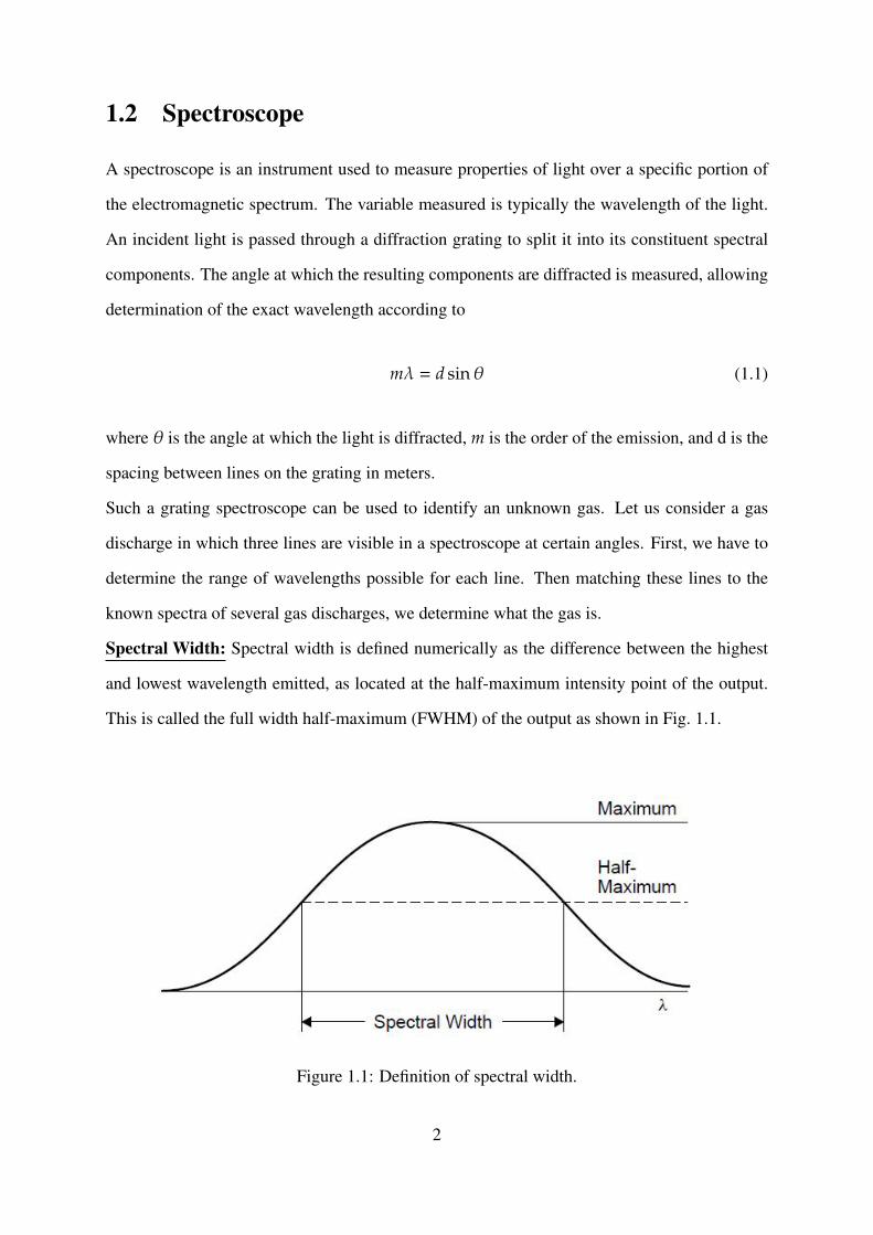
Spectral Width: Spectral width is defined numerically as the difference between the highest

and lowest wavelength emitted, as located at the half-maximum intensity point of the output.

This is called the full width half-maximum (FWHM) of the output as shown in Fig. 1.1.

Figure 1.1: Definition of spectral width.

2

A spectrally narrow line spans few wavelengths, while a broad source (such as blackbody

emission) spans a large range of wavelengths.

1.3 Einstein and Planck Relation: E = hν

In 1899, Max Planck assumed that the energy of any oscillator at a frequency ν could exist only

in discrete (quantized) units of hν, where h is a constant (called Plancks constant). Based on

this theory Einstein introduced the concept of the photon to be a little packet of light that have

energy proportional to their frequency and hence inversely proportional to their wavelength.

The mathematical expression of this energy is

E = hν =hcλ

(1.2)

where ν is the frequency, h is Planck’s constant, c is the speed of light and λ is the wavelength.

Using this relationship, one can easily measure the energy of an emitted photon from the line

spectra of an atom. For example, violet photons at 400 nm have an energy of 3 eV whereas red

photons at 700 nm have an energy of 1.8 eV.

1.4 Photoelectric Effect

The photoelectric effect provides proof of the relationship between energy and frequency as

brought to light in the Planck relationship. It also demonstrates the particle nature of light.

The effect is observed when photons of light strike a metal surface in a vacuum and electrons

are ejected in response to bombardment by these incident photons. The important findings of

this phenomena are:

• For a given metal, there exists a certain minimum frequency of incident radiation below

which no photoelectrons are emitted. This frequency is called the threshold frequency,

ν0.

3

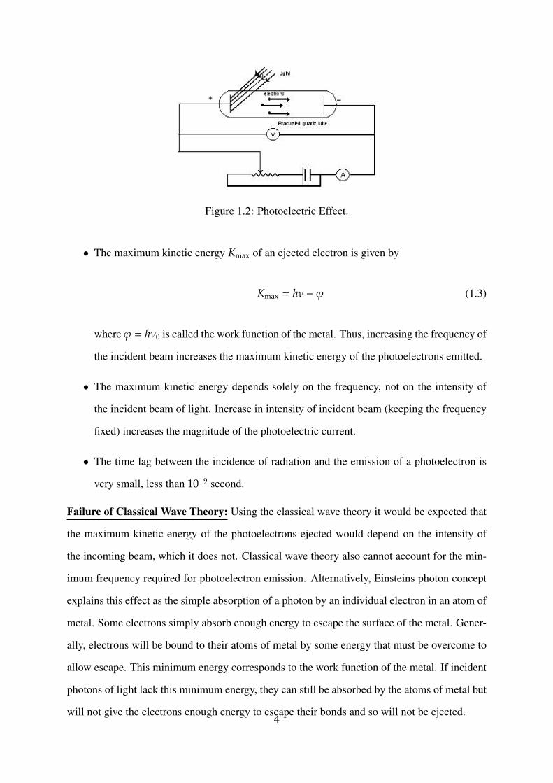
Figure 1.2: Photoelectric Effect.

• The maximum kinetic energy Kmax of an ejected electron is given by

Kmax = hν − ϕ (1.3)

where ϕ = hν0 is called the work function of the metal. Thus, increasing the frequency of

the incident beam increases the maximum kinetic energy of the photoelectrons emitted.

• The maximum kinetic energy depends solely on the frequency, not on the intensity of

the incident beam of light. Increase in intensity of incident beam (keeping the frequency

fixed) increases the magnitude of the photoelectric current.

• The time lag between the incidence of radiation and the emission of a photoelectron is

very small, less than 10−9 second.

Failure of Classical Wave Theory: Using the classical wave theory it would be expected that

the maximum kinetic energy of the photoelectrons ejected would depend on the intensity of

the incoming beam, which it does not. Classical wave theory also cannot account for the min-

imum frequency required for photoelectron emission. Alternatively, Einsteins photon concept

explains this effect as the simple absorption of a photon by an individual electron in an atom of

metal. Some electrons simply absorb enough energy to escape the surface of the metal. Gener-

ally, electrons will be bound to their atoms of metal by some energy that must be overcome to

allow escape. This minimum energy corresponds to the work function of the metal. If incident

photons of light lack this minimum energy, they can still be absorbed by the atoms of metal but

will not give the electrons enough energy to escape their bonds and so will not be ejected.4

1.5 Atomic Models and Light Emission

The Rutherford-Bohr atomic model can be used to explain the emission spectra seen in hydro-

gen gas. The model postulates that:

• Electrons around an atom orbit in a number of possible discrete energy states according

to the laws of Newtonian mechanics.

• The angular momentum of these orbiting electrons is quantized and limited to a set of

values, called the quantum number, which represents which orbit the electron is in.

• Atoms do not radiate energy as long as they are fixed in that orbit.

• Atoms may jump from one energy state to another and in doing so will emit radiation in

the form of a photon. The photon will contain the energy difference between the initial,

higher-energy state and the final, lower-energy state.

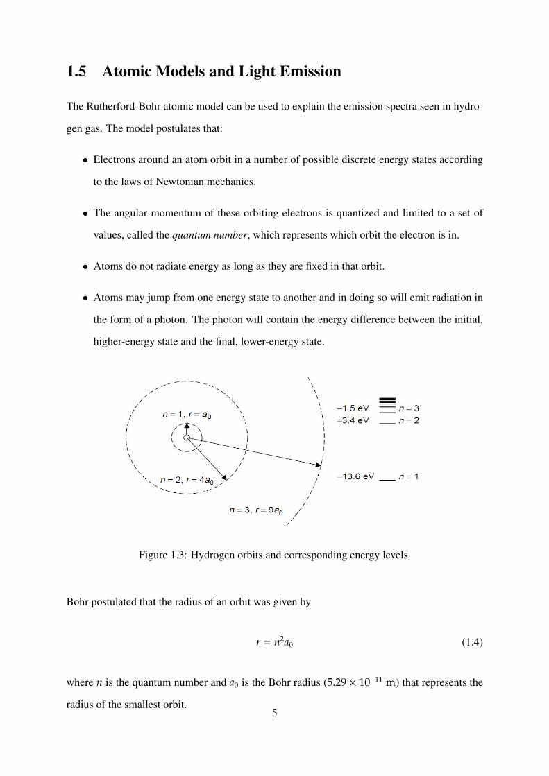
Figure 1.3: Hydrogen orbits and corresponding energy levels.

Bohr postulated that the radius of an orbit was given by

r = n2a0 (1.4)

where n is the quantum number and a0 is the Bohr radius (5.29 × 10−11 m) that represents the

radius of the smallest orbit.5

Energy of an electron in a particular orbit is given by

E = −13.6n2 (1.5)

where E is the energy in eV. Electrons in the first Bohr orbit have an energy of −13.6 eV. As

the quantum number increases, these levels get crowded closer together, as outlined in Fig. 1.3.

The emission spectrum of hydrogen consists of discrete lines, each of which can now be ex-

plained as corresponding with a jump or transition in the energy states of the atom. In the case

of the Balmer series, the final energy state is n = 2. Thus, the five visible lines of hydrogen

may now be seen as a jump between a higher-energy state with n = 3, 4, 5, 6, or7 and a lower-

energy state with n = 2. If the transitions between energy levels end at n = 1, these transitions

have very high energies, being so close to the nucleus, so photons emitted in transitions to this

final state have high energies. These lines are observed in the ultraviolet and are called the Ly-

man series. Other transitions may end with n = 3 and have lower-energy changes, so photons

emitted are in the infrared (the Paschen series).

1.6 Franck-Hertz Experiment

The FranckHertz experiment demonstrates the fact that energy levels in atoms are indeed quan-

tized into discrete levels.

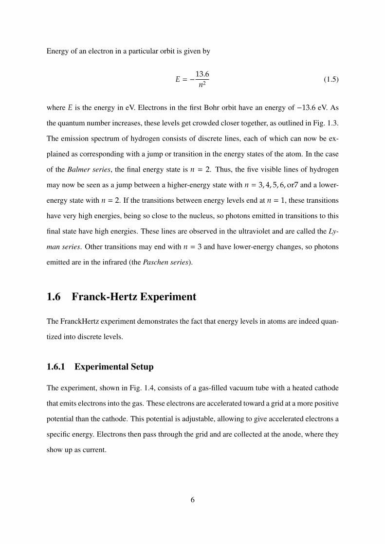
1.6.1 Experimental Setup

The experiment, shown in Fig. 1.4, consists of a gas-filled vacuum tube with a heated cathode

that emits electrons into the gas. These electrons are accelerated toward a grid at a more positive

potential than the cathode. This potential is adjustable, allowing to give accelerated electrons a

specific energy. Electrons then pass through the grid and are collected at the anode, where they

show up as current.

6

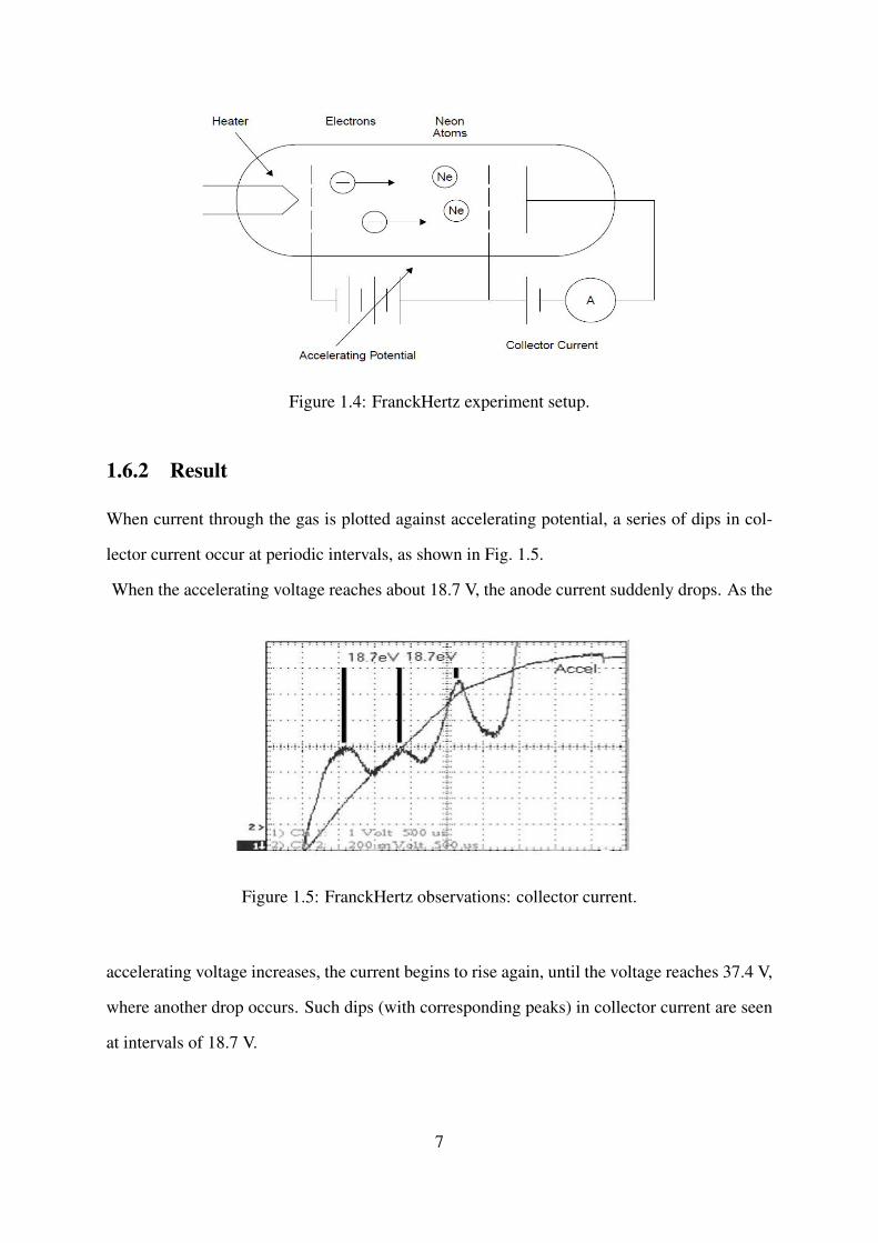
Figure 1.4: FranckHertz experiment setup.

1.6.2 Result

When current through the gas is plotted against accelerating potential, a series of dips in col-

lector current occur at periodic intervals, as shown in Fig. 1.5.

When the accelerating voltage reaches about 18.7 V, the anode current suddenly drops. As the

Figure 1.5: FranckHertz observations: collector current.

accelerating voltage increases, the current begins to rise again, until the voltage reaches 37.4 V,

where another drop occurs. Such dips (with corresponding peaks) in collector current are seen

at intervals of 18.7 V.

7

1.6.3 Interpretation of Result

The interpretation of this experiment is that electrons below 18.7 eV do not have enough energy

to excite the neon atom to an allowed energy and so pass through the gas unimpeded, being

manifested as current through the tube. At 18.7 eV the electrons have enough energy to excite

neon atoms to their first excited level upon impact. The result of the collision is that the energy

of the electron is totally absorbed by the much heavier atom, pushing the neon atom’s energy

to the first excited state. Since the energy of the neon atom is quantized, it can take on certain

allowed values only. Electrons whose energy is below 18.7 eV cannot transfer energy to the

neon atom to excite it. The corresponding drop in current occurs because electrons at that

energy are no longer flowing though the tube to the anode but rather, are transferring their

energy to neon atoms (where they show up as emitted light).

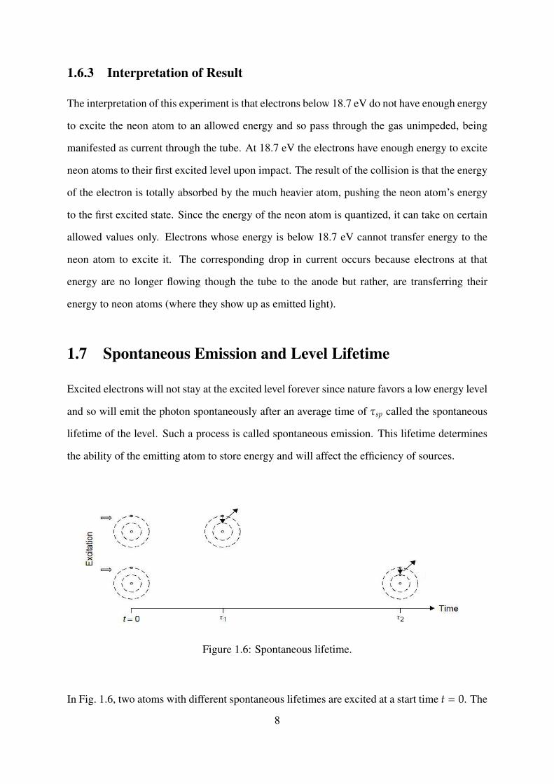
1.7 Spontaneous Emission and Level Lifetime

Excited electrons will not stay at the excited level forever since nature favors a low energy level

and so will emit the photon spontaneously after an average time of τsp called the spontaneous

lifetime of the level. Such a process is called spontaneous emission. This lifetime determines

the ability of the emitting atom to store energy and will affect the efficiency of sources.

Figure 1.6: Spontaneous lifetime.

In Fig. 1.6, two atoms with different spontaneous lifetimes are excited at a start time t = 0. The

8

top atom, with a relatively short lifetime, emits a photon spontaneously at a time t = τ1, while

the second atom, with a longer lifetime, waits until an elapsed time of t = τ2 before emitting a

photon.

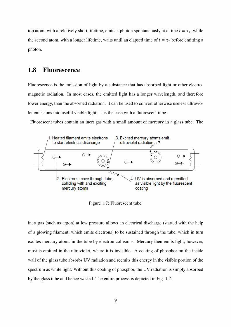
1.8 Fluorescence

Fluorescence is the emission of light by a substance that has absorbed light or other electro-

magnetic radiation. In most cases, the emitted light has a longer wavelength, and therefore

lower energy, than the absorbed radiation. It can be used to convert otherwise useless ultravio-

let emissions into useful visible light, as is the case with a fluorescent tube.

Fluorescent tubes contain an inert gas with a small amount of mercury in a glass tube. The

Figure 1.7: Fluorescent tube.

inert gas (such as argon) at low pressure allows an electrical discharge (started with the help

of a glowing filament, which emits electrons) to be sustained through the tube, which in turn

excites mercury atoms in the tube by electron collisions. Mercury then emits light; however,

most is emitted in the ultraviolet, where it is invisible. A coating of phosphor on the inside

wall of the glass tube absorbs UV radiation and reemits this energy in the visible portion of the

spectrum as white light. Without this coating of phosphor, the UV radiation is simply absorbed

by the glass tube and hence wasted. The entire process is depicted in Fig. 1.7.

9

1.9 Semiconductor Devices

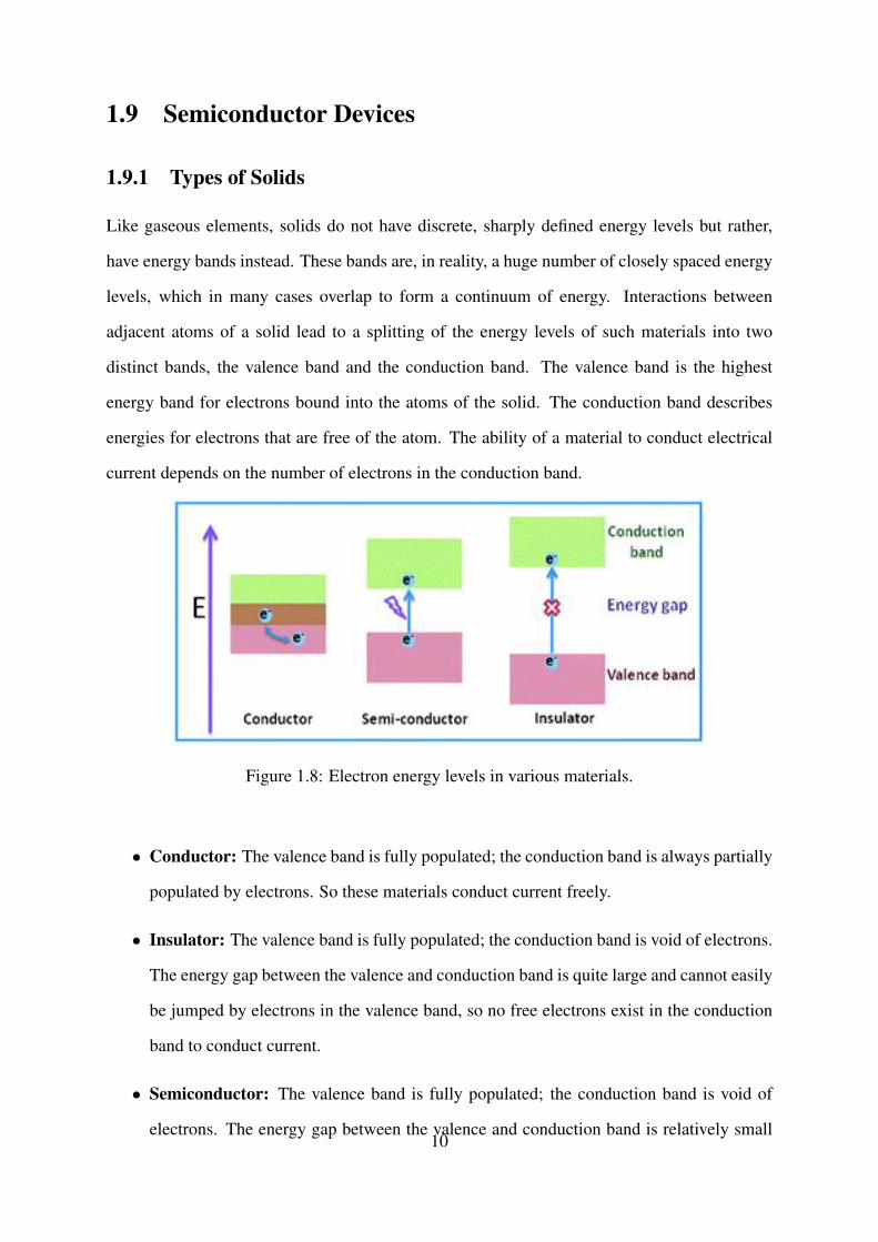
1.9.1 Types of Solids

Like gaseous elements, solids do not have discrete, sharply defined energy levels but rather,

have energy bands instead. These bands are, in reality, a huge number of closely spaced energy

levels, which in many cases overlap to form a continuum of energy. Interactions between

adjacent atoms of a solid lead to a splitting of the energy levels of such materials into two

distinct bands, the valence band and the conduction band. The valence band is the highest

energy band for electrons bound into the atoms of the solid. The conduction band describes

energies for electrons that are free of the atom. The ability of a material to conduct electrical

current depends on the number of electrons in the conduction band.

Figure 1.8: Electron energy levels in various materials.

• Conductor: The valence band is fully populated; the conduction band is always partially

populated by electrons. So these materials conduct current freely.

• Insulator: The valence band is fully populated; the conduction band is void of electrons.

The energy gap between the valence and conduction band is quite large and cannot easily

be jumped by electrons in the valence band, so no free electrons exist in the conduction

band to conduct current.

• Semiconductor: The valence band is fully populated; the conduction band is void of

electrons. The energy gap between the valence and conduction band is relatively small10

and electrons may be made to jump the gap between the bands, at which point the free

electron is mobile and the material can carry current.

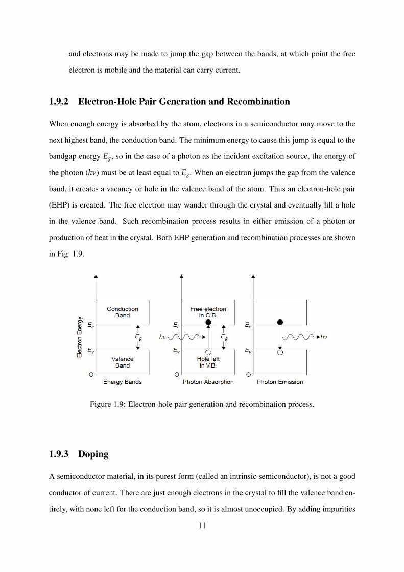
1.9.2 Electron-Hole Pair Generation and Recombination

When enough energy is absorbed by the atom, electrons in a semiconductor may move to the

next highest band, the conduction band. The minimum energy to cause this jump is equal to the

bandgap energy Eg, so in the case of a photon as the incident excitation source, the energy of

the photon (hν) must be at least equal to Eg. When an electron jumps the gap from the valence

band, it creates a vacancy or hole in the valence band of the atom. Thus an electron-hole pair

(EHP) is created. The free electron may wander through the crystal and eventually fill a hole

in the valence band. Such recombination process results in either emission of a photon or

production of heat in the crystal. Both EHP generation and recombination processes are shown

in Fig. 1.9.

Figure 1.9: Electron-hole pair generation and recombination process.

1.9.3 Doping

A semiconductor material, in its purest form (called an intrinsic semiconductor), is not a good

conductor of current. There are just enough electrons in the crystal to fill the valence band en-

tirely, with none left for the conduction band, so it is almost unoccupied. By adding impurities

11

to the semiconductor (a process called doping) it can be made to have an excess of electrons

which will then populate the conduction band.

• Adding dopants such as phosphorus or arsenic creates a type of semiconductor with

excess electrons (in the conduction band) called n-type semiconductor.

• Adding dopants such as boron creates a type of semiconductor with excess holes (in the

valence band) called p-type semiconductor.

1.9.4 p-n Junction

A pn junction is formed at the boundary between a p-type and n-type semiconductor. After

joining p-type and n-type semiconductors, electrons near the pn interface tend to diffuse into

the p region. Likewise, holes near the pn interface begin to diffuse into the n-type region. Thus

the regions nearby the pn interfaces lose their neutrality and become charged, forming the space

charge region or depletion layer.

Figure 1.10: A p-n junction in thermal equilibrium with zero-bias voltage applied.

The electric field created by the space charge region opposes the diffusion process for both12

electrons and holes. There are two concurrent phenomena: the diffusion process that tends to

generate more space charge, and the electric field generated by the space charge that tends to

counteract the diffusion. An equilibrium is reached between these two processes.

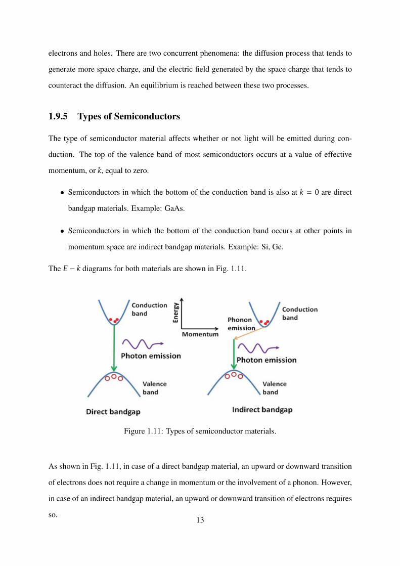
1.9.5 Types of Semiconductors

The type of semiconductor material affects whether or not light will be emitted during con-

duction. The top of the valence band of most semiconductors occurs at a value of effective

momentum, or k, equal to zero.

• Semiconductors in which the bottom of the conduction band is also at k = 0 are direct

bandgap materials. Example: GaAs.

• Semiconductors in which the bottom of the conduction band occurs at other points in

momentum space are indirect bandgap materials. Example: Si, Ge.

The E − k diagrams for both materials are shown in Fig. 1.11.

Figure 1.11: Types of semiconductor materials.

As shown in Fig. 1.11, in case of a direct bandgap material, an upward or downward transition

of electrons does not require a change in momentum or the involvement of a phonon. However,

in case of an indirect bandgap material, an upward or downward transition of electrons requires

so.13

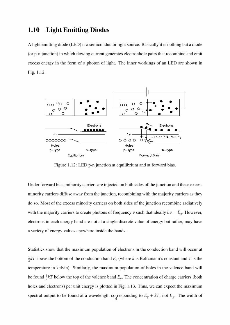
1.10 Light Emitting Diodes

A light emitting diode (LED) is a semiconductor light source. Basically it is nothing but a diode

(or p-n junction) in which flowing current generates electronhole pairs that recombine and emit

excess energy in the form of a photon of light. The inner workings of an LED are shown in

Fig. 1.12.

Figure 1.12: LED p-n junction at equilibrium and at forward bias.

Under forward bias, minority carriers are injected on both sides of the junction and these excess

minority carriers diffuse away from the junction, recombining with the majority carriers as they

do so. Most of the excess minority carriers on both sides of the junction recombine radiatively

with the majority carriers to create photons of frequency ν such that ideally hν = Eg. However,

electrons in each energy band are not at a single discrete value of energy but rather, may have

a variety of energy values anywhere inside the bands.

Statistics show that the maximum population of electrons in the conduction band will occur at

12kT above the bottom of the conduction band Ec (where k is Boltzmann’s constant and T is the

temperature in kelvin). Similarly, the maximum population of holes in the valence band will

be found 12kT below the top of the valence band Ev. The concentration of charge carriers (both

holes and electrons) per unit energy is plotted in Fig. 1.13. Thus, we can expect the maximum

spectral output to be found at a wavelength corresponding to Eg + kT, not Eg. The width of14

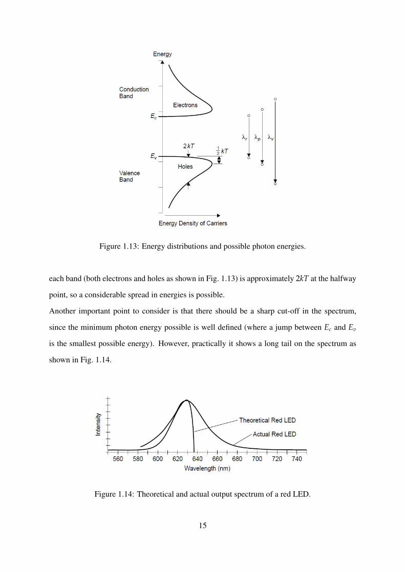
Figure 1.13: Energy distributions and possible photon energies.

each band (both electrons and holes as shown in Fig. 1.13) is approximately 2kT at the halfway

point, so a considerable spread in energies is possible.

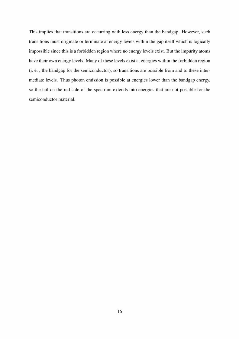
Another important point to consider is that there should be a sharp cut-off in the spectrum,

since the minimum photon energy possible is well defined (where a jump between Ec and Ev

is the smallest possible energy). However, practically it shows a long tail on the spectrum as

shown in Fig. 1.14.

Figure 1.14: Theoretical and actual output spectrum of a red LED.

15

This implies that transitions are occurring with less energy than the bandgap. However, such

transitions must originate or terminate at energy levels within the gap itself which is logically

impossible since this is a forbidden region where no energy levels exist. But the impurity atoms

have their own energy levels. Many of these levels exist at energies within the forbidden region

(i. e. , the bandgap for the semiconductor), so transitions are possible from and to these inter-

mediate levels. Thus photon emission is possible at energies lower than the bandgap energy,

so the tail on the red side of the spectrum extends into energies that are not possible for the

semiconductor material.

16

Chapter 2

Quantum Mechanics

There are many phenomena involving light such as the UV catastrophe, photoelectric effect,

origin of line spectra in which classical physics is inadequate to describe completely. Thus

quantum mechanics has been developed to account for effects seen at the subatomic level which

simply cannot be described through classical theory. One of the major outcome of this is the

realization that clearly there is more to energy levels than simply a principal quantum number.

2.1 Limitations of the Bohr Model

The major limitations of the Bohr model are:

• It only works with simple atoms having only a single valence electron. It does not work

for a complex atom such as neon (which has six electrons in its outer shell) or even for

helium (which has two electrons in its outer shell).

• According to Bohr theory, the ground state of hydrogen (n = 1) has orbital angular

momentum. But when quantum states for hydrogen are considered in detail, it can be

proved that the ground state of hydrogen has zero angular momentum.

17

2.2 Wave Properties of Particles (Duality)

The photoelectric effect has proved that electromagnetic radiation, which was generally thought

as a wave, can behave like particles also. The converse is also true. A particle can exhibit wave

behavior. In 1924, Louis deBroglie attempted to calculate the wavelength associated with a

particle. By combining the Planck-Einstein relation for photons, E = hν with Einstein’s mass-

to-energy equivalency, E = mc2, we can obtain,

hν = mc2 (2.1)

Substituting for ν = c/λ, we get

λ =h

mc(2.2)

Replacing p = mc (p is the momentum) in the above equation results into

λ =hp

(2.3)

Thus, a particle with momentum p can exhibit a wave like behavior with wavelength λ.

2.3 Evidence of Wave Properties in Electrons

In Young’s double slit experiment, we get the proof of wave nature of light. In 1928, physicist

G. P. Thomson attempted the same experiment, with electrons instead of light. First, using

electrons accelerated by high voltage, a collimated beam of electrons was produced with a

deBroglie wavelength of 0.01 nm. Extremely thin gold foil was used as a crystal, which would

diffract the electron beam as it passed through. The pattern produced was a striking circular

diffraction pattern showing without a doubt that electrons were diffracting and hence exhibiting

wave behavior. Furthermore, it was shown that magnetic and electrical fields would affect the

pattern, proving that the particle exiting the foil was indeed a charged electron.

In the electron double-slit experiment, diffraction pattern is still produced even when the beam

18

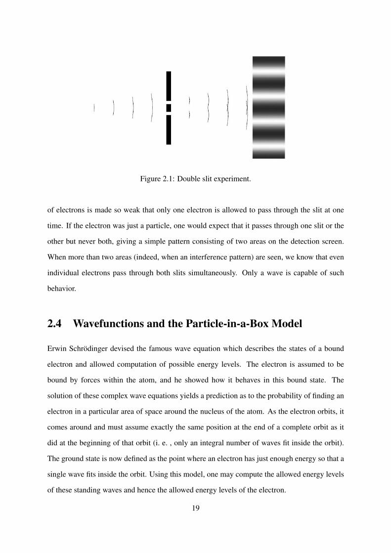
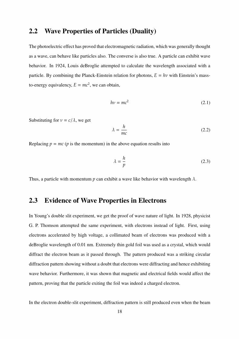
Figure 2.1: Double slit experiment.

of electrons is made so weak that only one electron is allowed to pass through the slit at one

time. If the electron was just a particle, one would expect that it passes through one slit or the

other but never both, giving a simple pattern consisting of two areas on the detection screen.

When more than two areas (indeed, when an interference pattern) are seen, we know that even

individual electrons pass through both slits simultaneously. Only a wave is capable of such

behavior.

2.4 Wavefunctions and the Particle-in-a-Box Model

Erwin Schrodinger devised the famous wave equation which describes the states of a bound

electron and allowed computation of possible energy levels. The electron is assumed to be

bound by forces within the atom, and he showed how it behaves in this bound state. The

solution of these complex wave equations yields a prediction as to the probability of finding an

electron in a particular area of space around the nucleus of the atom. As the electron orbits, it

comes around and must assume exactly the same position at the end of a complete orbit as it

did at the beginning of that orbit (i. e. , only an integral number of waves fit inside the orbit).

The ground state is now defined as the point where an electron has just enough energy so that a

single wave fits inside the orbit. Using this model, one may compute the allowed energy levels

of these standing waves and hence the allowed energy levels of the electron.

19

Figure 2.2: Model of a particle in a box.

Let us consider a box whose sides represent energy potentials that confine the electron. We

can describe the behavior of the electron in orbit by the wavefunction ψ which in this case is

a simple sine function. At the edges of the box, the wavefunction must be equal to zero since

it is a standing wave. By substituting integers into the wavefunction, we may identify many

possible modes for such a wave among which three are shown in Fig. 2.2. Each mode will have

a successively higher energy and in-between modes (those that do not have an integral number

of wavelengths inside the box) cannot exist. This model fits well with observed quantizations

of energy levels in atoms.

2.5 Reconciling Classical and Quantum Mechanics

The conclusions regarding the use of classical and quantum mechanics can be summarized as:

• Classical physics such as Newtonian mechanics provides a very clear view of how macro-

scopic particles and everyday objects behave.

• Depending on the circumstances, quantum physics may best describe the properties and

behaviors of subatomic particles such as electrons.

• At large quantum numbers, quantum mechanics simply reduces to classical physics.20

2.6 Angular Momentum in Quantum States

A charged electron has two types of angular momentum: orbital and spin. It generates a mag-

netic field by virtue of the fact that it is a moving charge. Spin is an intrinsic property of

electrons and is manifested by the magnetic moment created by spinning electrons. Like other

quantities in an atom, angular momentum is also quantized into allowed values.

One major shortcoming of the Bohr model was the failure to account for the hyperfine structure

of hydrogen lines. Each line emitted from hydrogen is, in fact, a series of very closely spaced

lines. A set of allowed orbits, for orbital and spin momentum, would exist for each principal

quantum number n. Thus transitions between these closely spaced energy levels give rise to the

many closely spaced lines seen in hydrogen spectra.

Orbital Quantum Number: It describes the magnitude of the orbital angular momentum and

is represented by l. l can have integer values of zero to n − 1. For example, for a principal

quantum number of n = 2, l can be 0 or 1, meaning that an electron in the n = 2 state can have

zero angular momentum, corresponding to a circular orbit, or some discrete value of angular

momentum, corresponding to an elliptical orbit.

2.7 Spectroscopic Notation and Electron Configuration

For any given value of n, there are a number of possible states of l, and each value of l is as-

signed a letter as follows:

Sharp s l = 0Principal p l = 1Diffuse d l = 2

Fundamental f l = 3

Higher order states after l = 3 continue with consecutive letters g, h, i, and so on.

In quantum mechanics an electron having a particular energy can be described as having a good

probability of being in a certain defined area. The 1s orbital, for example, has the appearance of

a sphere around the nucleus. As we move toward electron states with more angular momentum21

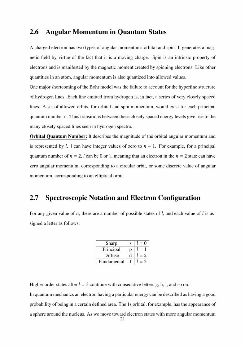
(i. e. , p and d orbitals), these probability distributions often take the form of lobes and toruses

around the nucleus. Three of them are shown in Fig. 2.3.

Figure 2.3: Probability distributions for various orbitals.

Each value of l represents an electron orbital, and each can hold a maximum number of elec-

trons before it is completely filled. Once filled, additional electrons will begin to fill the next

highest orbital based on order of energy. An s orbital can hold a maximum of two electrons, a

p orbital a maximum of six electrons, a d orbital a maximum of 10 electrons, and an f orbital

a maximum of 14 electrons. As an example, the electron configuration of sodium atom, which

has 11 electrons, is 1s22s22p63s1.

Transitions can occur between any energy state to yield photon emission, and unlike the Bohr

model, where electrons could be in only one principal quantum state (n = 2, n = 3, etc.), many

more levels are now available because with angular momentum now in the picture, each level

of n will now have n possible values of l.

2.8 Energy Levels Described by Orbital Angular

Momentum

By Bohr theory, we would expect that all electrons in an n = 2 state have exactly the same

energy, regardless of orbital configuration. This is not the case, and electrons in various orbital

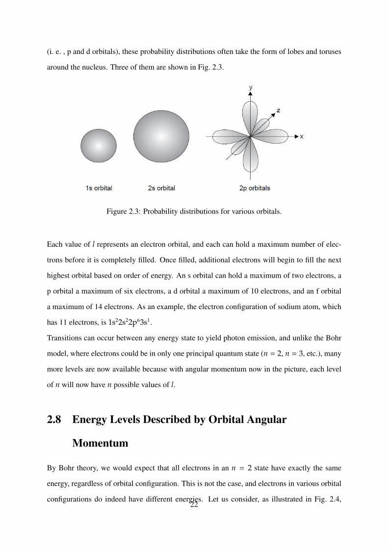
configurations do indeed have different energies. Let us consider, as illustrated in Fig. 2.4,22

atoms of hydrogen and sodium, each with a single electron in the outer shell.

Figure 2.4: Energy shells and levels in hydrogen and sodium.

At first instinct the energies of electrons in the outer shell of the sodium atom should be calcu-

lable by the same methodology as Bohr applied to the hydrogen atom. Spectroscopic studies,

however, reveal that electrons in the n = 3 orbit have significantly lower energies than electrons

of the hydrogen atom in the same n = 3 orbit. The orbit energy of n = 3 state of hydrogen

is -1.5 eV. The comparable orbit in the sodium atom is the 3s orbit (ground state for sodium),

which in this case has an energy of -5.0 eV, which is even lower than hydrogen’s n = 2 orbit

energy.

The reason for the shift in energy levels is attributed to a shielding effect of the completed inner

shells, which serve to lower the energy of the levels outside these. In effect, the inner shells,

complete with all electrons, prevent the solitary electron in the outer shell from feeling the full

attraction of the positive nucleus of the atom. The farther away these outer-shell electrons are

from the nucleus, the more closely their energies match those of the electron in the hydrogen

atom at the same state.

2.9 Magnetic Quantum Numbers

An electron with angular momentum is analogous to a current loop and will exhibit a magnetic

moment. This magnetic moment is denoted by the magnetic quantum number m. It represents23

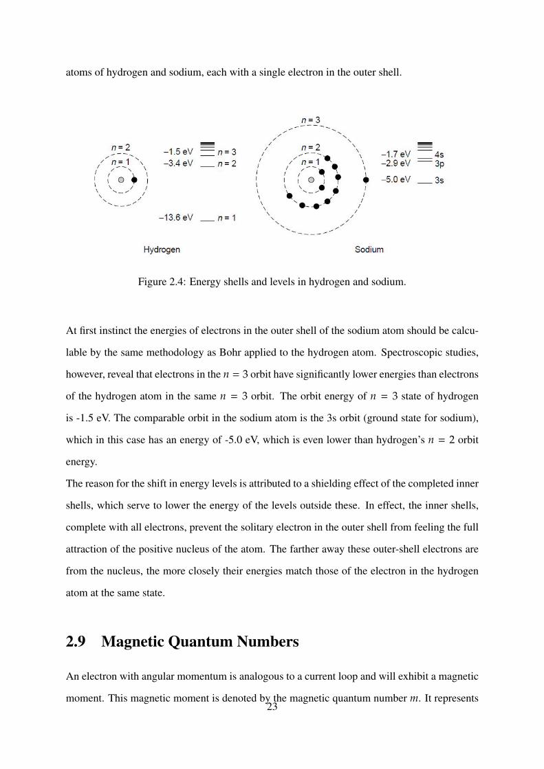
the direction of angular momentum of an electron. It can be thought of as the three-dimensional

tilt of an elliptical orbit, as depicted in Fig. 2.5.

Figure 2.5: Representation of the magnetic quantum number.

This number may assume integer values ranging from −l to +l. For example, an s orbital with

l = 0 always assumes a magnetic quantum number of m = 0, while a p orbital with l = 1 can

have numbers m = −1, 0,+1. In all, there are 2l + 1 possible values for m for a given value of

l.

2.10 Direct Evidence of Momentum:

The Stern-Gerlach Experiment

This experiment shows that angular momentum is indeed quantized and can be described by an

integer quantity (i. e. , it could only assume certain allowed values). The experiment, depicted

in Fig. 2.6, involves the deflection of a beam of neutral silver atoms emerging from a hot oven

via a magnetic field and onto the target of a photographic plate. The beam of atoms is directed

through an inhomogeneous magnetic field whose field could be varied and directed toward a

photographic plate, where it could be detected.

24

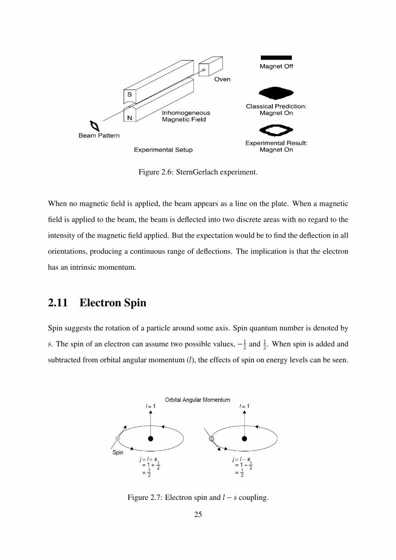
Figure 2.6: SternGerlach experiment.

When no magnetic field is applied, the beam appears as a line on the plate. When a magnetic

field is applied to the beam, the beam is deflected into two discrete areas with no regard to the

intensity of the magnetic field applied. But the expectation would be to find the deflection in all

orientations, producing a continuous range of deflections. The implication is that the electron

has an intrinsic momentum.

2.11 Electron Spin

Spin suggests the rotation of a particle around some axis. Spin quantum number is denoted by

s. The spin of an electron can assume two possible values, −12 and 1

2 . When spin is added and

subtracted from orbital angular momentum (l), the effects of spin on energy levels can be seen.

Figure 2.7: Electron spin and l − s coupling.

25

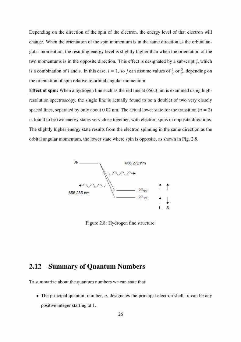
Depending on the direction of the spin of the electron, the energy level of that electron will

change. When the orientation of the spin momentum is in the same direction as the orbital an-

gular momentum, the resulting energy level is slightly higher than when the orientation of the

two momentums is in the opposite direction. This effect is designated by a subscript j, which

is a combination of l and s. In this case, l = 1, so j can assume values of 12 or 3

2 , depending on

the orientation of spin relative to orbital angular momentum.

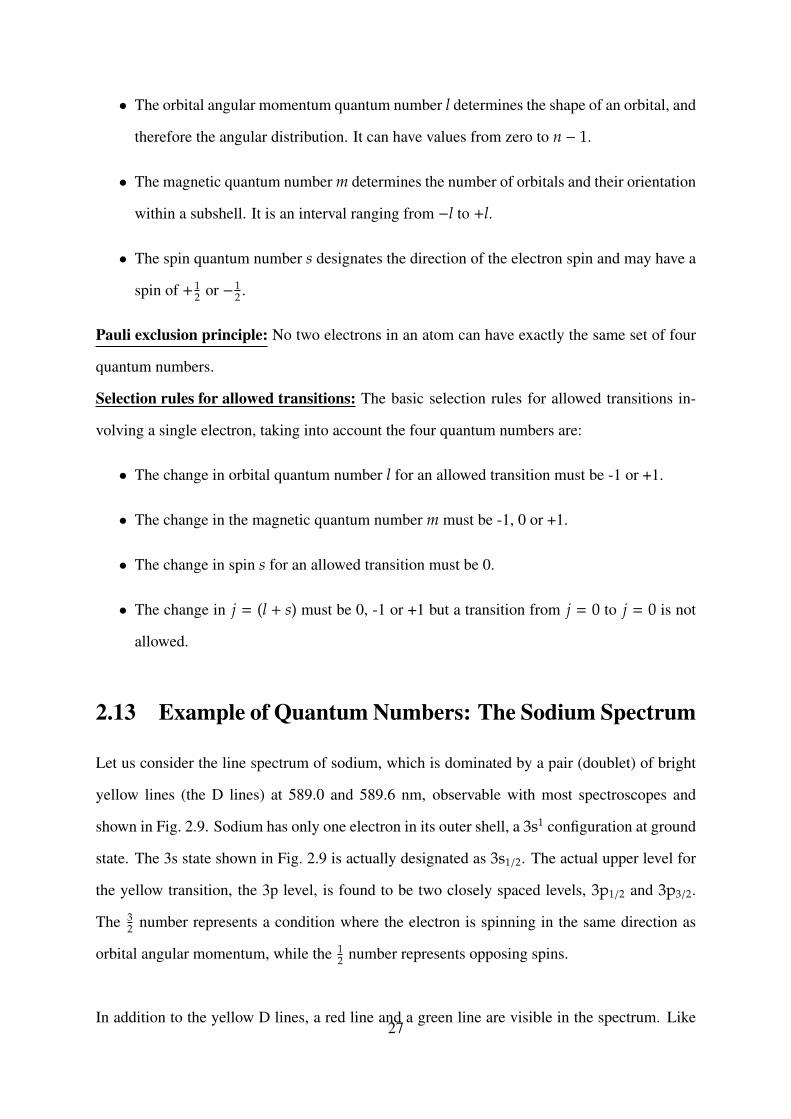
Effect of spin: When a hydrogen line such as the red line at 656.3 nm is examined using high-

resolution spectroscopy, the single line is actually found to be a doublet of two very closely

spaced lines, separated by only about 0.02 nm. The actual lower state for the transition (n = 2)

is found to be two energy states very close together, with electron spins in opposite directions.

The slightly higher energy state results from the electron spinning in the same direction as the

orbital angular momentum, the lower state where spin is opposite, as shown in Fig. 2.8.

Figure 2.8: Hydrogen fine structure.

2.12 Summary of Quantum Numbers

To summarize about the quantum numbers we can state that:

• The principal quantum number, n, designates the principal electron shell. n can be any

positive integer starting at 1.

26

• The orbital angular momentum quantum number l determines the shape of an orbital, and

therefore the angular distribution. It can have values from zero to n − 1.

• The magnetic quantum number m determines the number of orbitals and their orientation

within a subshell. It is an interval ranging from −l to +l.

• The spin quantum number s designates the direction of the electron spin and may have a

spin of + 12 or − 1

2 .

Pauli exclusion principle: No two electrons in an atom can have exactly the same set of four

quantum numbers.

Selection rules for allowed transitions: The basic selection rules for allowed transitions in-

volving a single electron, taking into account the four quantum numbers are:

• The change in orbital quantum number l for an allowed transition must be -1 or +1.

• The change in the magnetic quantum number m must be -1, 0 or +1.

• The change in spin s for an allowed transition must be 0.

• The change in j = (l + s) must be 0, -1 or +1 but a transition from j = 0 to j = 0 is not

allowed.

2.13 Example of Quantum Numbers: The Sodium Spectrum

Let us consider the line spectrum of sodium, which is dominated by a pair (doublet) of bright

yellow lines (the D lines) at 589.0 and 589.6 nm, observable with most spectroscopes and

shown in Fig. 2.9. Sodium has only one electron in its outer shell, a 3s1 configuration at ground

state. The 3s state shown in Fig. 2.9 is actually designated as 3s1/2. The actual upper level for

the yellow transition, the 3p level, is found to be two closely spaced levels, 3p1/2 and 3p3/2.

The 32 number represents a condition where the electron is spinning in the same direction as

orbital angular momentum, while the 12 number represents opposing spins.

In addition to the yellow D lines, a red line and a green line are visible in the spectrum. Like27

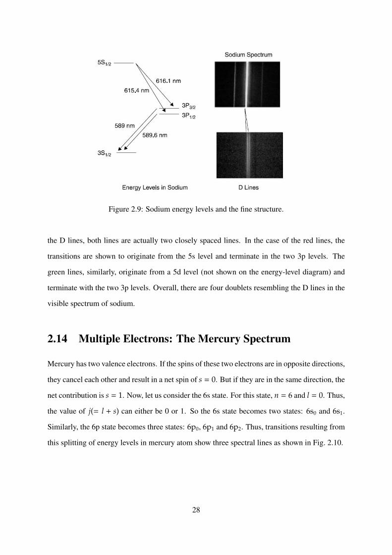
Figure 2.9: Sodium energy levels and the fine structure.

the D lines, both lines are actually two closely spaced lines. In the case of the red lines, the

transitions are shown to originate from the 5s level and terminate in the two 3p levels. The

green lines, similarly, originate from a 5d level (not shown on the energy-level diagram) and

terminate with the two 3p levels. Overall, there are four doublets resembling the D lines in the

visible spectrum of sodium.

2.14 Multiple Electrons: The Mercury Spectrum

Mercury has two valence electrons. If the spins of these two electrons are in opposite directions,

they cancel each other and result in a net spin of s = 0. But if they are in the same direction, the

net contribution is s = 1. Now, let us consider the 6s state. For this state, n = 6 and l = 0. Thus,

the value of j(= l + s) can either be 0 or 1. So the 6s state becomes two states: 6s0 and 6s1.

Similarly, the 6p state becomes three states: 6p0, 6p1 and 6p2. Thus, transitions resulting from

this splitting of energy levels in mercury atom show three spectral lines as shown in Fig. 2.10.

28

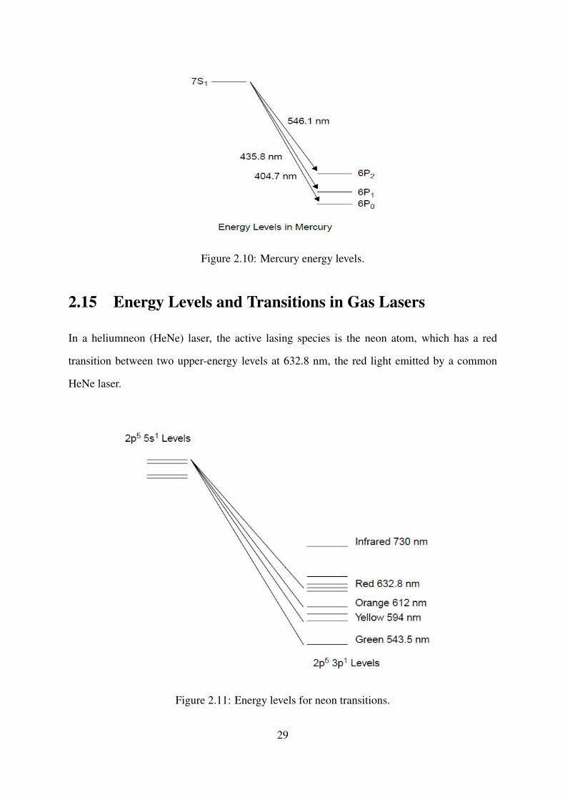
Figure 2.10: Mercury energy levels.

2.15 Energy Levels and Transitions in Gas Lasers

In a heliumneon (HeNe) laser, the active lasing species is the neon atom, which has a red

transition between two upper-energy levels at 632.8 nm, the red light emitted by a common

HeNe laser.

Figure 2.11: Energy levels for neon transitions.

29

A neon atom at ground state has an electron configuration of 1s22s22p6. It is an inert gas in

that all outer orbitals are filled, so it is not reactive. If neon is excited sufficiently, it can achieve

a level of 1s22s22p55s1. From that level it can fall to the 1s22s22p53p1 level and in doing so

emit a photon of red light at 632.8 nm. This is the transition used for the red HeNe laser.The

upper level (2p55s1) is actually four hyperfine levels, and the lower level (2p53p1), 10 separate

levels. As a result, there are numerous transitions at which the heliumneon laser can operate.

Some transitions are favored over others, and not all will produce laser light.

2.16 Molecular Energy Levels

Apart from the electronic transitions from various energy levels, other energy levels possible

are vibrational and rotational levels in molecules due to various supported modes of movements

of individual atoms relative to each other. For example, a diatomic molecule such as nitrogen

or hydrogen is composed of two atoms which are free to vibrate only in certain allowed ways.

Shared bonds, called covalent bonds, are formed between their atoms with electrons of oppos-

ing spin. This molecular bond is not rigid but rather, is flexible and may be stretched in various

ways as the atoms move. Different motions require different energies, which correspond to

photon energies in the electromagnetic spectrum.

2.16.1 Example: Hydrogen Molecule

Allowed modes of vibration (and hence corresponding energy levels) of hydrogen atom are de-

picted in Fig. 2.12. As the nuclei of the two hydrogen atoms deviate from the normal separation

for a hydrogen molecule, the energy increases and the vibrational mode (denoted by ν in the

figure) increases because a molecule with more energy tends to vibrate more. Transitions can

take place between two of these vibrational levels, resulting in a purely vibrational transition

with energies corresponding to transitions in the infrared region.

30

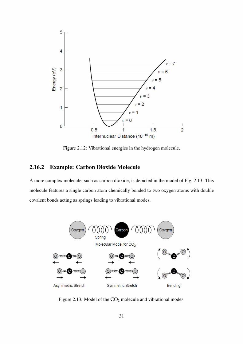
Figure 2.12: Vibrational energies in the hydrogen molecule.

2.16.2 Example: Carbon Dioxide Molecule

A more complex molecule, such as carbon dioxide, is depicted in the model of Fig. 2.13. This

molecule features a single carbon atom chemically bonded to two oxygen atoms with double

covalent bonds acting as springs leading to vibrational modes.

Figure 2.13: Model of the CO2 molecule and vibrational modes.

31

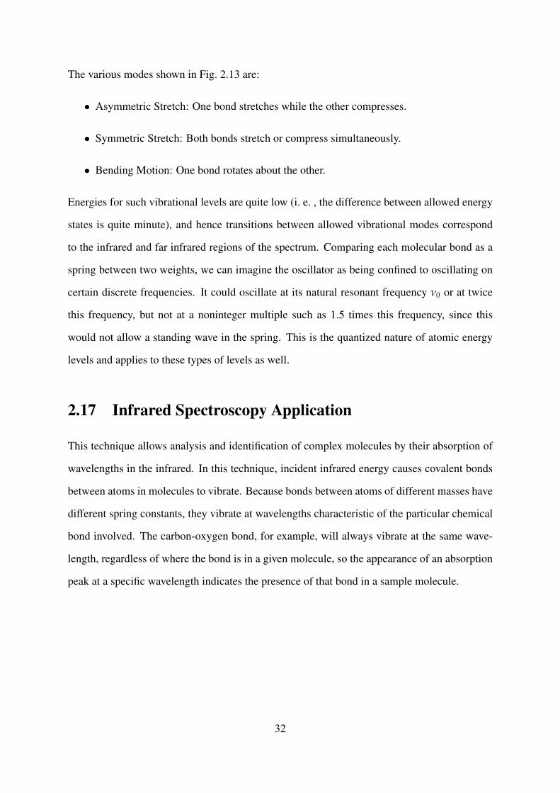
The various modes shown in Fig. 2.13 are:

• Asymmetric Stretch: One bond stretches while the other compresses.

• Symmetric Stretch: Both bonds stretch or compress simultaneously.

• Bending Motion: One bond rotates about the other.

Energies for such vibrational levels are quite low (i. e. , the difference between allowed energy

states is quite minute), and hence transitions between allowed vibrational modes correspond

to the infrared and far infrared regions of the spectrum. Comparing each molecular bond as a

spring between two weights, we can imagine the oscillator as being confined to oscillating on

certain discrete frequencies. It could oscillate at its natural resonant frequency ν0 or at twice

this frequency, but not at a noninteger multiple such as 1.5 times this frequency, since this

would not allow a standing wave in the spring. This is the quantized nature of atomic energy

levels and applies to these types of levels as well.

2.17 Infrared Spectroscopy Application

This technique allows analysis and identification of complex molecules by their absorption of

wavelengths in the infrared. In this technique, incident infrared energy causes covalent bonds

between atoms in molecules to vibrate. Because bonds between atoms of different masses have

different spring constants, they vibrate at wavelengths characteristic of the particular chemical

bond involved. The carbon-oxygen bond, for example, will always vibrate at the same wave-

length, regardless of where the bond is in a given molecule, so the appearance of an absorption

peak at a specific wavelength indicates the presence of that bond in a sample molecule.

32