audiometry using realistic sound scenes - aalto-yliopisto
TRANSCRIPT

Teemu Koski
Audiometry Using Realistic SoundScenes Reproduced with ParametricSpatial Audio
School of Electrical Engineering
Thesis submitted for examination for the degree of Master ofScience in Technology.
Espoo 19.3.2012
Thesis supervisor:
Docent Ville Pulkki
Thesis instructor:
D.Sc. (Tech.) Ville Sivonen
A! Aalto UniversitySchool of ElectricalEngineering

aalto university
school of electrical engineering
abstract of the
master’s thesis
Author: Teemu Koski
Title: Audiometry Using Realistic Sound Scenes Reproduced with ParametricSpatial Audio
Date: 19.3.2012 Language: English Number of pages:11+81
Department of Signal Processing and Acoustics
Professorship: Acoustics and Audio Signal Processing Code: S-89
Supervisor: Docent Ville Pulkki
Instructor: D.Sc. (Tech.) Ville Sivonen
The term audiometry denotes the testing of hearing performance. It is convention-ally conducted by measuring the hearing thresholds for pure tones over headphones.However, especially hearing-impaired individuals and hearing instrument users gener-ally have the most problems in communication situations where background noise ispresent. Results from pure-tone audiometry do not necessarily describe these problemswell. To better assess the real-life hearing performance, sound-field audiometry (SFA)systems have been developed, in which loudspeakers are used instead of headphones.Speech and real or synthetic background noise materials are typically used in SFA sys-tems. However, most of the current SFA systems are either too large and complex forclinical environments or do not reproduce the spatial characteristics of the sound scenecorrectly.Directional Audio Coding (DirAC) is a parametric spatial sound reproduction technique,which utilizes the knowledge on the temporal and spectral resolution of human hearing.With DirAC, the spatial attributes of sound can be captured and reproduced witharbitrary loudspeaker setups.In this thesis, DirAC was applied to audiometric purposes. A sound-field audiometrysystem was proposed, with which speech intelligibility assessments can be done in real-istic pre-recorded sound scenes where external test speech is augmented. With acousticmeasurements and psychoacoustic listening tests, a comparison was made between areference sound scene and a reproduced scene where the reference was reproduced bythe method under investigation. The main result was that speech intelligibility did notdiffer notably between the reference and the proposed system. This was confirmed inlistening tests conducted with both a group of normal hearing test subjects and a groupconsisting of cochlear implant and hearing aid users. The results suggested that theproposed method is valid for clinical hearing diagnostics. The main advantage of thesystem is that it enables the assessments of real-life hearing abilities using a relativelycompact loudspeaker setup. Requirements were specified for a clinical implementationof the system, considering the loudspeaker setup and the test room acoustics.
Keywords: Psychoacoustics, audiology, sound-field audiometry, spatial sound, para-metric spatial audio, DirAC
aalto-yliopisto
sahkotekniikan korkeakoulu
diplomityon
tiivistelma
Tekija: Teemu Koski
Tyon nimi: Audiometria realistisissa aaniymparistoissa parametristatilaaanentoistoa kayttaen
Paivamaara: 19.3.2012 Kieli: Englanti Sivumaara:11+81
Signaalinkasittelyn ja akustiikan laitos
Professuuri: Akustiikka ja aanenkasittelytekniikka Koodi: S-89
Valvoja: Dosentti Ville Pulkki
Ohjaaja: TkT Ville Sivonen
Audiometria tarkoittaa kuulon toiminnan tutkimista. Perinteinen metodi on aanes-audiometria, jossa potilaan kuulokynnys mitataan siniaaneksilla kuulokkeita kayttaen.Kuulovammaiset ja kuulolaitteen kayttajat kuitenkin tyypillisesti kokevat hankalimpinakommunikaatiotilanteet taustamelussa. Aanesaudiometria ei mittaa naita ongelmiakunnolla. Aanikenttaaudiometriassa kaytetaan kaiuttimia kuulokkeiden sijaan, jol-loin kuulon kaytannon suorituskykya voi mitata paremmin. Tallaisissa jarjestelmissakaytetaan testimateriaalina tyypillisesti puhetta seka aanitettya tai synteettista taus-tamelua. Useimmat nykyisista aanikenttaaudiometriatoteutuksista tosin ovat joko liiansuuria ja kompleksisia kliinisiin ymparistoihin tai eivat toista aanen tilaominaisuuksiakunnolla.Directional Audio Coding (DirAC) on parametrinen tilaaanen analysointi- ja toistotek-niikka, joka hyodyntaa tietoa ihmisen kuulon aika- ja taajuusresoluutiosta. DirAC:navulla aanen tilaan liittyvat ominaisuudet voidaan tallentaa ja toistaa mielivaltaisellakaiutinjarjestelmalla.Tassa tyossa sovellettiin DirAC:a audiometriaan. Tyossa esiteltiin aanikenttaaudio-metriasovellus, jonka avulla kuulon diagnostiikkaa voidaan tehda realistisissa ennaltaaanitetyissa aaniymparistoissa, joihin on augmentoitu ulkoista testipuhetta. Refer-enssiaaniymparistoa ja sen DirAC-toistettua kopiota verrattiin keskenaan akustisin mit-tauksin ja psykoakustisin kuuntelukokein. Paatulos oli, etta puheenymmarrettavyysei poikennut merkittavasti naiden ymparistojen valilla. Tama todistettiin kuun-telukokein, joissa koehenkiloina kaytettiin seka normaalikuuloisia etta kuulolaitteenja sisakorvaistutteen kayttajia. Ehdotettua metodia voi tulosten perustella kayttaakuulon diagnostiikkaan klinikkaymparistossa. Sovelluksen tarkein etu on sen tuo-ma mahdollisuus mitata kuulon tosielaman suorituskykya verrattain kompaktillakaiutinjarjestelmalla. Jarjestelman tekniset vaatimukset maariteltiin kaiutinjarjestel-man ja testihuoneen akustiikan osalta.
Avainsanat: Psykoakustiikka, audiologia, aanikenttaaudiometria, tilaaani, parametri-nen tilaaanentoisto, DirAC
Acknowledgements
This research in this thesis was conducted in the Department of Signal Processing andAcoustics at the Aalto University School of Electrical Engineering. The research receivedfunding from the Academy of Finland, project number 121252.
First of all, I want to thank my supervisor Ville Pulkki from Aalto University and myinstructor Ville Sivonen from Cochlear Nordic AB for guidance, ideas and support. I alsoowe thanks to my workmates for the advice and comments – in addition to the refreshingmoments by the Fußball table. Special thanks go to Marko Takanen for the commentson data analysis, as well as Tapani Pihlajamaki, Mikko-Ville Laitinen, Javier Gomez,Archontis Politis, and Olli Rummukainen for the advice on various practicalities.
I would also like to give a warm hug to my family and especially my beloved Pauliina forsupporting me in whatever I end up doing. Finally, additional hi-fives go to my friendsand bandmates for providing me counterbalance during the research process.
Otaniemi, 19.3.2012
Teemu J. Koski
iv

Contents
Abstract . . . . . . . . . . . . . . . . . . . . . . . . . . . . . . . . . . . . . . . . . iiAbstract (in Finnish) . . . . . . . . . . . . . . . . . . . . . . . . . . . . . . . . . . iiiAcknowledgements . . . . . . . . . . . . . . . . . . . . . . . . . . . . . . . . . . . ivContents . . . . . . . . . . . . . . . . . . . . . . . . . . . . . . . . . . . . . . . . . vAbbreviations . . . . . . . . . . . . . . . . . . . . . . . . . . . . . . . . . . . . . . viiiList of Figures . . . . . . . . . . . . . . . . . . . . . . . . . . . . . . . . . . . . . ixList of Tables . . . . . . . . . . . . . . . . . . . . . . . . . . . . . . . . . . . . . . xi
1 Introduction 11.1 Background . . . . . . . . . . . . . . . . . . . . . . . . . . . . . . . . . . . . 11.2 Aim of the thesis . . . . . . . . . . . . . . . . . . . . . . . . . . . . . . . . . 21.3 Outline of the thesis . . . . . . . . . . . . . . . . . . . . . . . . . . . . . . . 2
2 Sound and hearing 32.1 Sound as a phenomenon . . . . . . . . . . . . . . . . . . . . . . . . . . . . . 32.2 Sound in rooms . . . . . . . . . . . . . . . . . . . . . . . . . . . . . . . . . . 42.3 Auditory system . . . . . . . . . . . . . . . . . . . . . . . . . . . . . . . . . 62.4 Some attributes of hearing . . . . . . . . . . . . . . . . . . . . . . . . . . . . 9
2.4.1 Sensitivity of hearing . . . . . . . . . . . . . . . . . . . . . . . . . . . 92.4.2 Critical bands and masking . . . . . . . . . . . . . . . . . . . . . . . 10
2.5 Spatial hearing . . . . . . . . . . . . . . . . . . . . . . . . . . . . . . . . . . 122.5.1 General discussion . . . . . . . . . . . . . . . . . . . . . . . . . . . . 122.5.2 Binaural localization cues . . . . . . . . . . . . . . . . . . . . . . . . 132.5.3 Monaural localization cues . . . . . . . . . . . . . . . . . . . . . . . 142.5.4 Additional factors on localization . . . . . . . . . . . . . . . . . . . . 152.5.5 Binaural advantages in communication . . . . . . . . . . . . . . . . . 15
3 Techniques for spatial audio 173.1 Approaches to spatial audio reproduction . . . . . . . . . . . . . . . . . . . 17
3.1.1 Spatial audio with loudspeakers . . . . . . . . . . . . . . . . . . . . . 173.1.2 Spatial audio with headphones . . . . . . . . . . . . . . . . . . . . . 18
3.2 Directional Audio Coding (DirAC) . . . . . . . . . . . . . . . . . . . . . . . 193.2.1 The idea in brief . . . . . . . . . . . . . . . . . . . . . . . . . . . . . 193.2.2 A-format and B-format input signals . . . . . . . . . . . . . . . . . . 203.2.3 Limitations and drawbacks . . . . . . . . . . . . . . . . . . . . . . . 20
4 Overview of technical audiology 214.1 Hearing disorders . . . . . . . . . . . . . . . . . . . . . . . . . . . . . . . . . 21
v

vi
4.1.1 Types of hearing disorders . . . . . . . . . . . . . . . . . . . . . . . . 214.1.2 Conductive hearing loss . . . . . . . . . . . . . . . . . . . . . . . . . 224.1.3 Sensorineural hearing loss . . . . . . . . . . . . . . . . . . . . . . . . 224.1.4 Tinnitus and hyperacusis . . . . . . . . . . . . . . . . . . . . . . . . 25
4.2 Hearing instruments . . . . . . . . . . . . . . . . . . . . . . . . . . . . . . . 264.2.1 Hearing aid . . . . . . . . . . . . . . . . . . . . . . . . . . . . . . . . 264.2.2 Cochlear implant . . . . . . . . . . . . . . . . . . . . . . . . . . . . . 284.2.3 On hearing with hearing instruments . . . . . . . . . . . . . . . . . . 29
4.3 Hearing diagnostics . . . . . . . . . . . . . . . . . . . . . . . . . . . . . . . . 304.3.1 Pure-tone audiometry . . . . . . . . . . . . . . . . . . . . . . . . . . 304.3.2 Speech audiometry . . . . . . . . . . . . . . . . . . . . . . . . . . . . 324.3.3 Testing speech intelligibility in noise . . . . . . . . . . . . . . . . . . 33
4.4 Sound-field audiometry . . . . . . . . . . . . . . . . . . . . . . . . . . . . . . 354.4.1 Advantages of sound-field audiometry . . . . . . . . . . . . . . . . . 354.4.2 Test methods in sound field . . . . . . . . . . . . . . . . . . . . . . . 364.4.3 Technical considerations . . . . . . . . . . . . . . . . . . . . . . . . . 374.4.4 Sound field audiometer implementations . . . . . . . . . . . . . . . . 38
5 DirAC-based sound-field audiometry 415.1 The overall concept . . . . . . . . . . . . . . . . . . . . . . . . . . . . . . . . 415.2 Description of the SFA system . . . . . . . . . . . . . . . . . . . . . . . . . 42
5.2.1 Reproducing a sound scene . . . . . . . . . . . . . . . . . . . . . . . 425.2.2 Usage of the system in the test conductors viewpoint . . . . . . . . . 44
5.3 Prototyping . . . . . . . . . . . . . . . . . . . . . . . . . . . . . . . . . . . . 455.3.1 On the test environments . . . . . . . . . . . . . . . . . . . . . . . . 455.3.2 Reference environment . . . . . . . . . . . . . . . . . . . . . . . . . . 455.3.3 The listening room prototype setup . . . . . . . . . . . . . . . . . . 475.3.4 The anechoic prototype setup . . . . . . . . . . . . . . . . . . . . . . 47
5.4 Technical validation . . . . . . . . . . . . . . . . . . . . . . . . . . . . . . . 485.4.1 Sources of error in the reproduction chain . . . . . . . . . . . . . . . 485.4.2 Magnitude spectrum comparison . . . . . . . . . . . . . . . . . . . . 485.4.3 Informal observations from binaural recordings . . . . . . . . . . . . 495.4.4 Conclusions . . . . . . . . . . . . . . . . . . . . . . . . . . . . . . . . 50
6 Subjective listening tests 516.1 Test method in general . . . . . . . . . . . . . . . . . . . . . . . . . . . . . . 516.2 Test A . . . . . . . . . . . . . . . . . . . . . . . . . . . . . . . . . . . . . . . 52
6.2.1 Introduction . . . . . . . . . . . . . . . . . . . . . . . . . . . . . . . 526.2.2 Test subjects . . . . . . . . . . . . . . . . . . . . . . . . . . . . . . . 536.2.3 Test procedures . . . . . . . . . . . . . . . . . . . . . . . . . . . . . . 536.2.4 Results and analysis . . . . . . . . . . . . . . . . . . . . . . . . . . . 54
6.3 Test B . . . . . . . . . . . . . . . . . . . . . . . . . . . . . . . . . . . . . . . 566.3.1 Introduction . . . . . . . . . . . . . . . . . . . . . . . . . . . . . . . 566.3.2 Test subjects . . . . . . . . . . . . . . . . . . . . . . . . . . . . . . . 566.3.3 Test procedures . . . . . . . . . . . . . . . . . . . . . . . . . . . . . . 576.3.4 Results and analysis . . . . . . . . . . . . . . . . . . . . . . . . . . . 57
6.4 Test C . . . . . . . . . . . . . . . . . . . . . . . . . . . . . . . . . . . . . . . 596.4.1 Introduction . . . . . . . . . . . . . . . . . . . . . . . . . . . . . . . 59
vii
6.4.2 Test subjects . . . . . . . . . . . . . . . . . . . . . . . . . . . . . . . 596.4.3 Test procedures . . . . . . . . . . . . . . . . . . . . . . . . . . . . . . 596.4.4 Results and analysis . . . . . . . . . . . . . . . . . . . . . . . . . . . 60
6.5 Comparison of the results in tests A, B, and C . . . . . . . . . . . . . . . . 626.5.1 On the comparability of the results . . . . . . . . . . . . . . . . . . . 626.5.2 The effect of direct-to-reverberant ratio in the listening position . . . 626.5.3 The effect of the number of loudspeakers . . . . . . . . . . . . . . . . 636.5.4 The effect of test subject hearing performance . . . . . . . . . . . . . 63
6.6 Reliability of the results . . . . . . . . . . . . . . . . . . . . . . . . . . . . . 64
7 Discussion 667.1 Outcome of the listening tests . . . . . . . . . . . . . . . . . . . . . . . . . . 667.2 Evaluation of the DirAC-based SFA system . . . . . . . . . . . . . . . . . . 66
7.2.1 Validity . . . . . . . . . . . . . . . . . . . . . . . . . . . . . . . . . . 667.2.2 Advantages and drawbacks . . . . . . . . . . . . . . . . . . . . . . . 677.2.3 Suggestions for clinical implementations . . . . . . . . . . . . . . . . 67
7.3 Suggestions for further work . . . . . . . . . . . . . . . . . . . . . . . . . . . 68
8 Conclusion 70
Bibliography 76
A SPS200 Compensation filter 77
B Reverberation time measurement details 78
C Post-hoc analysis tables 79C.1 Test A . . . . . . . . . . . . . . . . . . . . . . . . . . . . . . . . . . . . . . . 79C.2 Test B . . . . . . . . . . . . . . . . . . . . . . . . . . . . . . . . . . . . . . . 80
D Direct-to-reverberant ratio measurement details 81

Abbreviations
BILD Binaural intelligibility level differenceBMLD Binaural masking level differenceCI Cochlear implantdB DecibeldBA Decibel (A-weighted)DirAC Directional Audio CodingDRR Direct-to-reverberant ratioHA Hearing aidHINT Hearing in noise testHL Hearing levelHRTF Head-related transfer functionHz HertzkHz KilohertzMILD Monaural intelligibility level differenceMLD Masking level differenceSFA Sound-field audiometrySNR Signal-to-noise ratioSPL Sound pressure levelSRM Spatial release from maskingSRT Speech recognition thresholdSRTN Speech recognition threshold in noisesSRT Sentence speech reception thresholdPTA Pure-tone audiometryVBAP Vector Base Amplitude PanningWFS Wave Field Synthesis
viii
List of Figures
2.1 Propagation of sound in rooms. . . . . . . . . . . . . . . . . . . . . . . . . . 52.2 A figure of the human ear. . . . . . . . . . . . . . . . . . . . . . . . . . . . . 62.3 A simplified schematic of the human ear. . . . . . . . . . . . . . . . . . . . . 62.4 A cross-section of the cochlea. . . . . . . . . . . . . . . . . . . . . . . . . . . 72.5 A simplified schematic of unfolded cochlea. . . . . . . . . . . . . . . . . . . 82.6 Tuning curves measured from individual auditory nerve fibers of cats. . . . 92.7 The human hearing range in terms of frequency and loudness. . . . . . . . . 102.8 The masking effect of a white noise masker for a pure tone test signal. . . . 112.9 Masking effect of a narrow-band masker. . . . . . . . . . . . . . . . . . . . . 112.10 Human localization ability in horizontal and median plane. . . . . . . . . . 122.11 Binaural localization cues visualized . . . . . . . . . . . . . . . . . . . . . . 13
3.1 The 5.1 standard specified in ITU-R BS.775-1. . . . . . . . . . . . . . . . . 18
4.1 An example of increased hearing thresholds due to hearing loss. . . . . . . . 234.2 Changes in the dynamic range of hearing due to sensorineural hearing loss. 254.3 Different types of hearing aids. . . . . . . . . . . . . . . . . . . . . . . . . . 274.4 A schematic of a cochlear implant. . . . . . . . . . . . . . . . . . . . . . . . 294.5 A pure tone audiogram visualizing hearing thresholds. . . . . . . . . . . . . 314.6 Simple loudspeaker arrangements for testing speech intelligibility in noise. . 364.7 The ”Simulated Open-Field Environment (SOFE)” system. . . . . . . . . . 394.8 The ”Virtual Sound Environment (VSE)” system. . . . . . . . . . . . . . . 40
5.1 The overall concept of DirAC-based sound-field audiometry. . . . . . . . . . 425.2 Block diagram of the DirAC-based SFA system. . . . . . . . . . . . . . . . . 435.3 The DirAC-based SFA system user interface for the test conductor. . . . . . 445.4 Sources of error in the SFA system reproduction chain. . . . . . . . . . . . . 485.5 Magnitude spectrum comparisons in the test environments. . . . . . . . . . 49
6.1 The listening test setups. . . . . . . . . . . . . . . . . . . . . . . . . . . . . 526.2 Test A results: individual SRT-scores. . . . . . . . . . . . . . . . . . . . . . 556.3 Test A results: marginal means and confidence intervals of the SRT-scores . 556.4 Test B results: individual SRT-scores. . . . . . . . . . . . . . . . . . . . . . 586.5 Test B results: marginal means and confidence intervals of the SRT-scores . 586.6 Test C results: individual SRT-scores. . . . . . . . . . . . . . . . . . . . . . 616.7 Test C results: marginal means and confidence intervals of the SRT-scores . 616.8 Comparison of the results in tests A and B. . . . . . . . . . . . . . . . . . . 626.9 Comparison of the results in tests B and C. . . . . . . . . . . . . . . . . . . 64
ix

x
A1 Magnitude responses of the Soundfield SPS200 microphone and the calcu-lated compensation filter. . . . . . . . . . . . . . . . . . . . . . . . . . . . . 77

List of Tables
5.1 Reverberation time and dimensions of the reference environment. . . . . . . 465.2 Dimensions and Schroeder frequency of the reference environment. . . . . . 465.3 Reverberation time and dimensions of the listening room prototype setup. . 475.4 Dimensions and Schroeder frequency of the listening room prototype setup. 47
6.1 ANOVA results for test A. . . . . . . . . . . . . . . . . . . . . . . . . . . . 546.2 ANOVA results for test B. . . . . . . . . . . . . . . . . . . . . . . . . . . . 576.3 Test subjects in test C: hearing loss types and hearing instrument types. . . 596.4 ANOVA results for test C. . . . . . . . . . . . . . . . . . . . . . . . . . . . 606.5 Direct-to-reverberant ratio in the listening room prototype setup. . . . . . . 63
C1 Post-hoc analysis results for test A. . . . . . . . . . . . . . . . . . . . . . . . 79C2 Post-hoc analysis results for test B. . . . . . . . . . . . . . . . . . . . . . . . 80
xi
Chapter 1
Introduction
1.1 Background
Modern living environments contain various kinds of sound information and noise. Thisemphasizes the importance of human ear to perform in its fundamental task: enablingcommunication in various sound scenes. High technology is being applied to hearinginstruments to make people cope with hearing disorders. Altogether, this situation em-phasizes the importance of reliable and representative hearing diagnostics.
The term audiometry denotes the testing of hearing performance and it can be conductedin several ways. Pure-tone audiometry over headphones is the conventional method: itgives the thresholds of hearing in different frequencies, which is a straightforward measureof how well the auditory system is reacting to sound. However, testing with pure tonesdoes not reflect the real-life hearing abilities: people with hearing impairments and usersof hearing instruments generally report to have the most problems in everyday communi-cation, where background noise and complicated room acoustics are present. Furthermore,headphone-listening is problematic and limited in several test cases.
An alternative approach for hearing diagnostics is sound-field audiometry (SFA), whereloudspeakers are used instead of headphones. In addition to solving the headphone-relatedproblems, sound-field audiometry allows testing the spatial aspects of hearing, which isessential in assessing the real-life hearing performance. In sound-field audiometry, speechintelligibility in the presence of a masking noise is an important measure. To measure this,setups have been proposed in which speech is reproduced from one loudspeaker and noisefrom another. However, these kind of two-loudspeaker approaches are limited in givingreliable and representative results. Recently, partly due to development in spatial soundtechnology, a growing interest has been to simulate real-life sound environments and roomacoustics for audiometric applications.
One recently developed technique for spatial audio is Directional Audio Coding (DirAC).It is a parametric spatial sound reproduction technique for arbitrary loudspeaker setups.DirAC is developed in Aalto University among its underlying techniques Spatial ImpulseResponse Rendering (SIRR) and Vector Base Amplitude Panning (VBAP). Although notapplied in the field of hearing diagnostics, these techniques have been shown applicable forexample to high-quality multi-channel audio and teleconferencing. Experiments in these
CHAPTER 1. INTRODUCTION 2
applications have shown good results even with setups consisting of relatively low numberof loudspeakers. This motivates the research on the use of these techniques in sound-fieldaudiometry.
1.2 Aim of the thesis
This thesis investigates the use of Directional Audio Coding for hearing diagnostics over aloudspeaker setup simple enough to be used in clinical environments. The initial aim is todesign a system for audiometric tests that could be used in clinical environments, bearing inmind the current needs and existing systems. The system would aim for assessing the real-life hearing performance and communication abilities relevant to the patient. Additionally,the functional gain of a hearing instrument could be measured with the system.
Besides the expected advantages, the use of spatial sound techniques in this applicationhighlights several considerations. Namely, DirAC utilizes some knowledge of the resolutionof human spatial hearing, and although it is well tested with normally-hearing listeners,the way how of hearing instrument users and hearing-impaired individuals perceive DirAC-reproduction is unclear. Furthermore, the SFA system to be designed should be compactenough for availability to clinical use, but at the same time accurate enough for reliableaudiometric testing. That is, a compromise has to be made between system versatility,reproduction accuracy, and the number of loudspeakers used. Indeed, reducing the numberof loudspeakers tends to lower the reproduction accuracy. This framework opens up a setof questions, which this thesis aims to answer:
• Is it relevant to conduct sound-field audiometry using real-life sound scenes re-produced with DirAC, while patients include both normally-hearing and hearing-impaired individuals and also hearing instrument users, and how could this be im-plemented?
• Could the reproduction be done with a setup compact enough to be used in clinicalenvironments, and what would be the technical requirements for the system then?
These questions are discussed through literature study, experimental engineering, acousticmeasurements, and psychoacoustic listening tests.
1.3 Outline of the thesis
This thesis divides roughly in two parts: the theory part of chapters 2–4 and the exper-imental part of chapters 5–7. Chapter 2 contains the principles of sound and hearing asprerequisites for the consequent chapters. Chapter 3 introduces spatial sound technologiesand describes Directional Audio Coding (DirAC). Chapter 4 gives an overview of hearingdefects, their management, and diagnosis, giving emphasis on sound-field audiometry. InChapter 5, a concept of a sound-field audiometry system featuring DirAC is developed,described and technically validated. Chapter 6 reports the conducted listening tests fur-ther validating the system. Chapter 7 summarizes the results of the experimental workand discusses the advantages, drawbacks and applicability of the proposed sound-fieldaudiometry system. Finally, Chapter 8 concludes the thesis.
Chapter 2
Sound and hearing
This chapter introduces the fundamental concepts of sound and hearing. These are bymuch preliminary information for the consequent chapters. Sections 2.1 and 2.2 aim atexplaining what sound is and how it behaves in different environments. Section 2.3 brieflyintroduces the human auditory system and the physiological basis for hearing. Sections 2.4and 2.5 explore the performance, range and limitations of hearing from different aspects.
2.1 Sound as a phenomenon
Sound, as described in [73], has two descriptions. In perceptual context, it means anauditory sensation in the auditory system. Sound can be wanted or unwanted: there isoften the wanted signal (e.g., speech) and also some unwanted noise (e.g.,, traffic noise).Physically, sound is longitudinal wave motion in a medium, which causes the auditorysensation. Similarly, noise has two meanings. While in perceptual context noise is anyunwanted or possibly harmful sound, physically noise is described as a waveform withrandom changes in instantaneous amplitude [92]. Signal to noise ratio (SNR) is definedas the level ratio between signal (i.e., meaningful information) and noise (i.e., unwantedsound) and is usually expressed in decibels (dB).
This thesis follows the terminology proposed in [8], as follows. Sound event is the physicalsound phenomenon, which can act as a stimulus (i.e., stimulate the auditory system).Auditory event or auditory object is the sound perceived by the listener. Sound scene isthe physical environment of sound, whereas auditory scene is its perceptual equivalent.The term sound environment is also used in this thesis to describe sound scenes moregenerally.
A sound wave is usually generated by some object, such as loudspeaker cone, vibratingmechanically and thus coupling the vibration to a medium, such as air. Other sound gener-ation mechanisms are changing airflow, rapidly changing heat sources and supersonic flow.Due to vibration, air particles move back and forth and thus generate pressure minimaand maxima. At fixed distance from the sound source, air pressure is oscillating aroundthe nominal air pressure. The amplitude of this oscillation is the sound pressure at thislocation. Sound pressure is usually denoted as a value relative to the reference pressure,which is approximately the smallest pressure amplitude that humans can perceive. This
3
CHAPTER 2. SOUND AND HEARING 4
relative measure, denoted in decibels, is called sound pressure level (SPL) and is definedas
Lp = 20 log10
(p
p0
)(2.1)
where p is the sound pressure and p0 is the reference pressure of 20 μPa. The wavelengthof a sound wave is the distance over which the wave is periodic, for example the distancebetween two pressure maxima. Frequency defines how many of these periods fits to onesecond. The relation between wavelength and frequency is defined as
f =λ
c(2.2)
where f is frequency, λ is wavelength and c is the speed of sound. The speed of sound inair is 344 m/s in temperature of 20◦C. [40, 73]
2.2 Sound in rooms
As a sound wave generated by a point source propagates freely in space, the sound pressuredecreases evenly, with inverse relation to the distance from the sound source. This isbecause the sound energy supplied by the source is spread to an increasing area as thedistance increases. Therefore, sound intensity, which is defined as the sound energy perunit area, is proportional to 1/r2, where r is the distance of the sound source. Soundpressure is then proportional to 1/r. Thus, by Equation 2.1, the sound pressure levelof a point source decreases linearly by 6 dB as the distance is doubled. This kind ofenvironment is called a free sound field or free field, where there are no boundaries forthe sound to reflect from. The opposite of a free field would be a diffuse field, where thesound is coming evenly from all directions. [73]
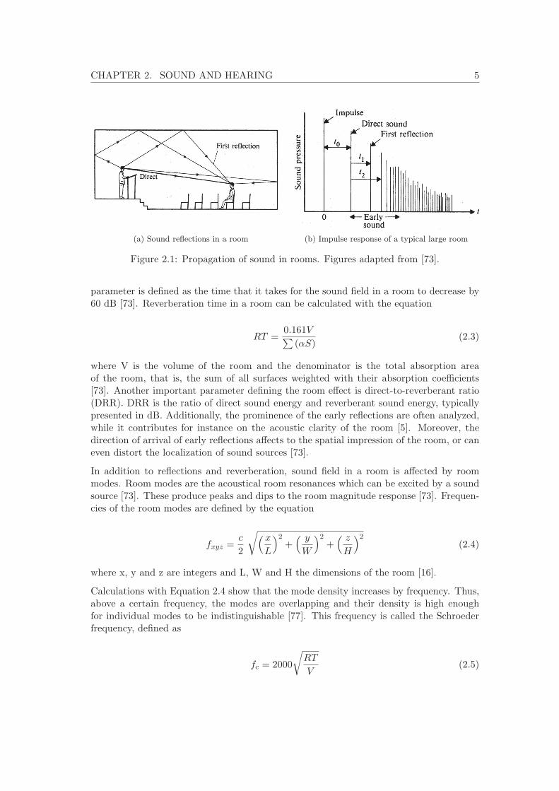
In an enclosed space, sound is encountered by objects and surfaces that partly reflect andpartly absorb the sound. The amount of how much of the sound energy is absorbed isdependent on the properties of the material and is depicted by the absorption coefficientα ∈ [0, 1]. Due to reflections, sound field in a room – from the viewpoint of the listener –can be separated to three components: direct sound, early reflections and late reflections.Figure 2.1a illustrates the paths of sound in a room. Direct sound is the first wavefrontthat reaches the ear of the listener. In a free field, this is the only sound that would reachthe listener. After the direct sound, the first reflections arrive from the walls, ceiling andfloor of the room. The reflections which arrive within the first 50–80 ms after the directsound are called the early reflections or the early sound. Soon the reflections arrive fromall directions and their temporal density is so high that individual reflections cannot bedistinguished. These are the late reflections that produce the late sound or reverberantsound. Figure 2.1b illustrates a simplified impulse response of a typical large room orauditorium, where these three components are visible. [73]
Room acoustics affect the perception of sound in a given room. The term room effect issometimes used to describe the contribution of the room to the resulting sound field andperception. A fundamental parameter in room acoustics is reverberation time (RT). This
CHAPTER 2. SOUND AND HEARING 5
(a) Sound reflections in a room (b) Impulse response of a typical large room
Figure 2.1: Propagation of sound in rooms. Figures adapted from [73].
parameter is defined as the time that it takes for the sound field in a room to decrease by60 dB [73]. Reverberation time in a room can be calculated with the equation
RT =0.161V∑
(αS)(2.3)
where V is the volume of the room and the denominator is the total absorption areaof the room, that is, the sum of all surfaces weighted with their absorption coefficients[73]. Another important parameter defining the room effect is direct-to-reverberant ratio(DRR). DRR is the ratio of direct sound energy and reverberant sound energy, typicallypresented in dB. Additionally, the prominence of the early reflections are often analyzed,while it contributes for instance on the acoustic clarity of the room [5]. Moreover, thedirection of arrival of early reflections affects to the spatial impression of the room, or caneven distort the localization of sound sources [73].
In addition to reflections and reverberation, sound field in a room is affected by roommodes. Room modes are the acoustical room resonances which can be excited by a soundsource [73]. These produce peaks and dips to the room magnitude response [73]. Frequen-cies of the room modes are defined by the equation
fxyz =c
2
√(x
L
)2+
( y
W
)2+
( z
H
)2(2.4)
where x, y and z are integers and L, W and H the dimensions of the room [16].
Calculations with Equation 2.4 show that the mode density increases by frequency. Thus,above a certain frequency, the modes are overlapping and their density is high enoughfor individual modes to be indistinguishable [77]. This frequency is called the Schroederfrequency, defined as
fc = 2000
√RT
V(2.5)
CHAPTER 2. SOUND AND HEARING 6
where V is the volume of the room [77]. In the context of room acoustics, Schroederfrequency is the crossover point above which a given room is acoustically large and theroom modes are negligible [16]. Below that point, the room is acoustically small andthe effect of room modes is prominent [16]. According to Equation 2.5, the Schroederfrequency increases as room volume decreases. Thereby, the room modes are essentiallyan issue of small rooms.
2.3 Auditory system
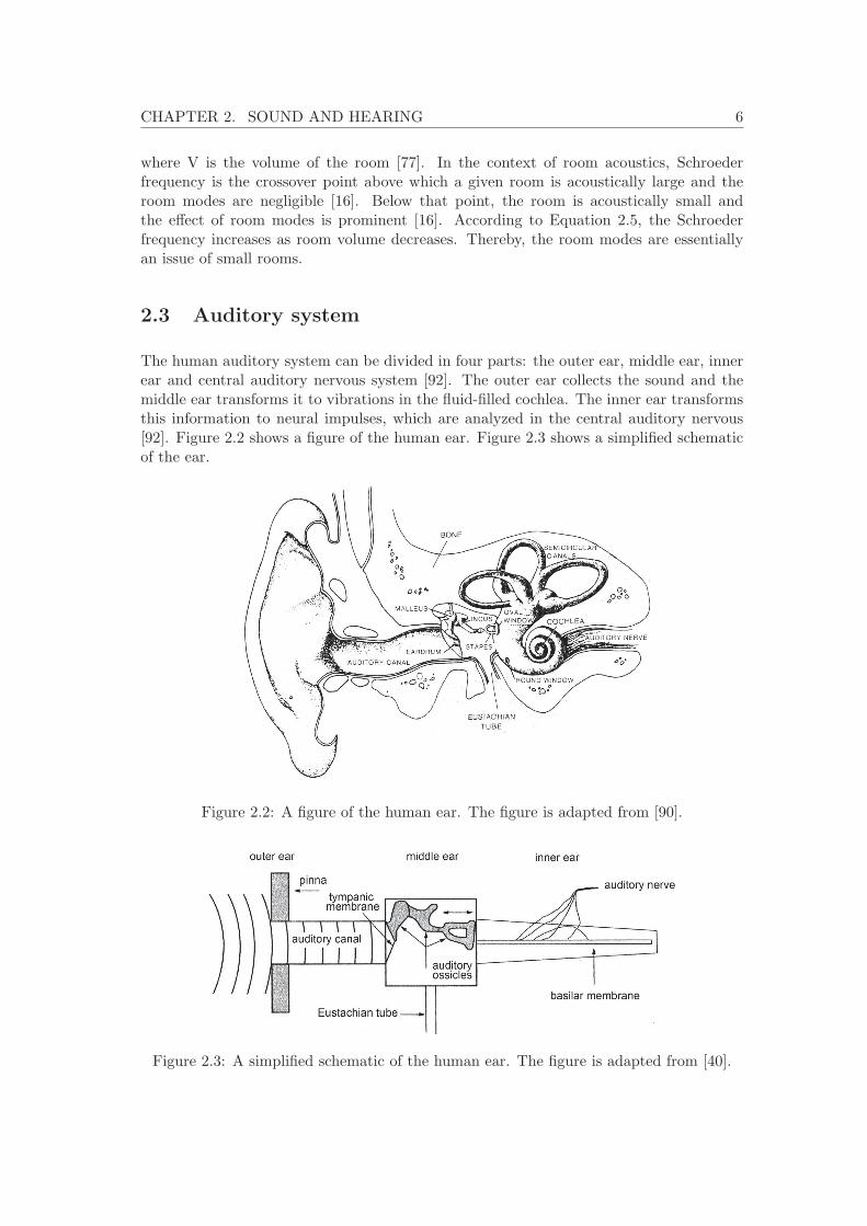
The human auditory system can be divided in four parts: the outer ear, middle ear, innerear and central auditory nervous system [92]. The outer ear collects the sound and themiddle ear transforms it to vibrations in the fluid-filled cochlea. The inner ear transformsthis information to neural impulses, which are analyzed in the central auditory nervous[92]. Figure 2.2 shows a figure of the human ear. Figure 2.3 shows a simplified schematicof the ear.
Figure 2.2: A figure of the human ear. The figure is adapted from [90].
Figure 2.3: A simplified schematic of the human ear. The figure is adapted from [40].
CHAPTER 2. SOUND AND HEARING 7
The outer ear is a passive and linear system that collects sound. It consists of the pinna,which is the visible part of the ear, and the auditory canal, which leads to the tympanicmembrane, also called the eardrum. The pinna has a complex and asymmetric shape,providing reflections, especially in high frequencies. The auditory canal acts as a resonatorwith a quarter-wavelength resonance between 2000–5500 Hz. Consequently, the humanhearing is relatively sensitive around this frequency range. The outer ear ends to thetympanic membrane, which vibrates with the sound pressure changes in the auditorycanal. [40]
The middle ear begins from the tympanic membrane. It consists of three auditory ossicles,namely malleus, incus and stapes, which connect the tympanic membrane to the cochleaof the inner ear. These bones act as an impedance transformer between the air in theouter ear and the fluid in the inner ear, thus enabling the vibration to transmit efficiently.[40]
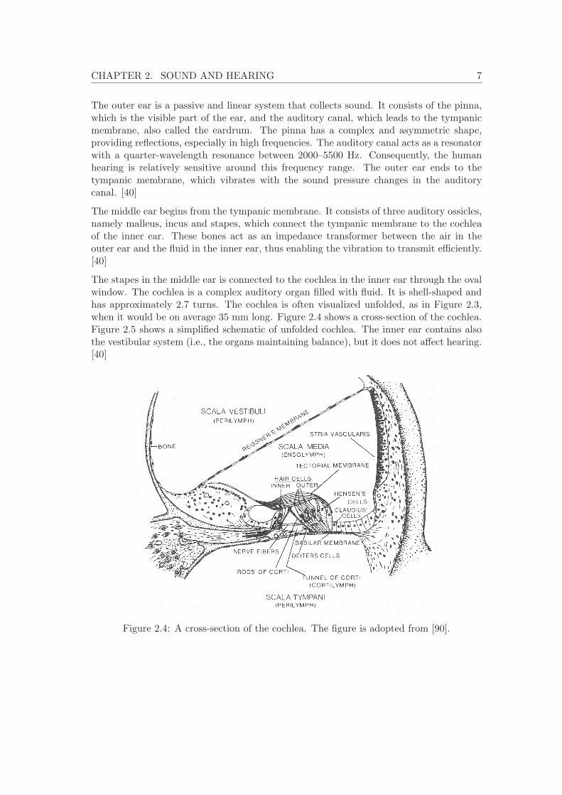
The stapes in the middle ear is connected to the cochlea in the inner ear through the ovalwindow. The cochlea is a complex auditory organ filled with fluid. It is shell-shaped andhas approximately 2.7 turns. The cochlea is often visualized unfolded, as in Figure 2.3,when it would be on average 35 mm long. Figure 2.4 shows a cross-section of the cochlea.Figure 2.5 shows a simplified schematic of unfolded cochlea. The inner ear contains alsothe vestibular system (i.e., the organs maintaining balance), but it does not affect hearing.[40]
Figure 2.4: A cross-section of the cochlea. The figure is adopted from [90].

CHAPTER 2. SOUND AND HEARING 8
Figure 2.5: A simplified schematic of unfolded cochlea. The figure is adapted from [40].
Vibrations transmitted by the stapes are coupled to the fluid of the cochlea and furtherto the basilar membrane. In the basilar membrane, there is the organ of Corti, whichcontains approximately 20000–30000 hair cells, equally placed over the membrane. Twotypes of hair cells exist, namely outer and inner hair cells. Inner hair cells, total of 3500,are in one row, whereas outer hair cells are in several rows. The hair cells transform thevibration of the basilar membrane to impulses and send them to the auditory nerve fibers.The neural impulse density is proportional to the vibration amplitude of the hair cells,but not linearly: with high vibration inputs, the impulse density output saturates. [40]
The nonlinear transfer function of hair cells shows that signal compression is taken placein the inner ear. According to [42], the outer hair cells act as a biomechanical gain controlthat provides compression. Furthermore, as stated for example in [42, 56], the outer haircells react to quiet sound levels and are more fragile than the inner hair cells. According to[41], there are more descending than ascending nerve fibers connected to outer hair cells,whereas to inner hair cells it is the opposite. Thus, the inner hair cells are the primaryreceptors collecting auditory information, whereas outer hair cells control the movementof the basilar membrane [41].
The basilar membrane can be thought as a spectrum analyzer. The basilar membrane isnarrow and light near the oval window, but thickens towards the end [40]. This affectsthe mechanical impedance seen by a traveling wave in the fluid. Therefore, hair cellsare frequency-selective depending on their position on the basilar membrane: the cellsin the beginning of the membrane react more to high frequencies and the cells in theend respectively more to low frequencies [40]. This frequency-selectivity is visualized bytuning curves, shown in Figure 2.6. A single tuning curve represents the level of inputstimulus needed at different frequencies for a constant output at an individual nerve fiber[40]. Thereby, tuning curves represent the frequency-specific sensitivities of individual haircells [40]. Figure 2.6 shows that the curves are somewhat wide and overlapping rather thanspinous. That is, even a pure tone1 excites not only one hair cell but an area in the basilarmembrane.
1A pure tone consists of only one frequency component and it’s spectrum is thus a spike in this frequency.

CHAPTER 2. SOUND AND HEARING 9
Figure 2.6: Tuning curves measured from individual auditory nerve fibers of cats. Thefigure is adapted from [40].
From the inner ear, sound information continues to the central auditory nervous system.First, the neural impulses from the cochlea travel to the cochlear nucleus, where it seemsthat the spectral processing is taken place. The next connection, from the cochlear nucleusto the superior olive, is both contralateral and ipsilateral. Consequently, the superior oliveis stimulated by both ears, enabling the analysis of the differences in the signals from bothsides. From the superior olive, the pathway continues to the inferior colliculus. However,there are also connections straight from the cochlear nucleus to the inferior colliculus.From inferior colliculus the pathway continues via medial geniculate body to auditorycortex, where the information is interpreted. [92]
2.4 Some attributes of hearing
2.4.1 Sensitivity of hearing
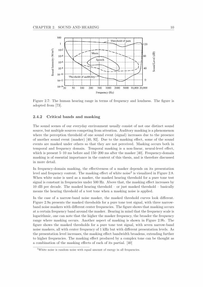
The human hearing range is limited in frequency and level, as visualized in Figure 2.7.In frequency, hearing ranges approximately from 20 Hz to 20 kHz. Sound loud enoughbelow 20 Hz can be sensed as vibration. In level, the dynamic range of hearing is betweenthe hearing threshold and the threshold of pain [73]. Hearing threshold of a young personis approximately p0 = 20 μPa, which is 0 dB in hearing level (HL) at 1 kHz. Below thethreshold of pain, there is loudness discomfort level, above which some distortion of soundmay occur [38]. The level of loudness discomfort varies individually.
CHAPTER 2. SOUND AND HEARING 10
Figure 2.7: The human hearing range in terms of frequency and loudness. The figure isadopted from [73].
2.4.2 Critical bands and masking
The sound scenes of our everyday environment usually consist of not one distinct soundsource, but multiple sources competing from attention. Auditory masking is a phenomenonwhere the perception threshold of one sound event (signal) increases due to the presenceof another sound event (masker) [40, 92]. Due to the masking effect, some of the soundevents are masked under others so that they are not perceived. Masking occurs both intemporal and frequency domain. Temporal masking is a non-linear, neural-level effect,which is present 5–10 ms before and 150–200 ms after the masker [40]. Frequency-domainmasking is of essential importance in the context of this thesis, and is therefore discussedin more detail.
In frequency-domain masking, the effectiveness of a masker depends on its presentationlevel and frequency content. The masking effect of white noise2 is visualized in Figure 2.8.When white noise is used as a masker, the masked hearing threshold for a pure tone testsignal is constant in frequencies under 500 Hz. Above that, the masking effect increases by10 dB per decade. The masked hearing threshold – or just masked threshold – basicallymeans the hearing threshold of a test tone when a masking noise is applied.
In the case of a narrow-band noise masker, the masked threshold curves look different.Figure 2.9a presents the masked thresholds for a pure tone test signal, with three narrow-band noise maskers with different center frequencies. The figure shows that masking occursat a certain frequency band around the masker. Bearing in mind that the frequency scale islogarithmic, one can note that the higher the masker frequency, the broader the frequencyrange where masking occurs. Another aspect of masking is shown in Figure 2.9b. Thefigure shows the masked thresholds for a pure tone test signal, with seven narrow-bandnoise maskers, all with center frequency of 1 kHz but with different presentation levels. Asthe presentation level increases, the masking effect bandwidth broadens, extending furtherto higher frequencies. The masking effect produced by a complex tone can be thought asa combination of the masking effects of each of its partial. [40]
2White noise is random noise with equal amount of energy in all frequencies.

CHAPTER 2. SOUND AND HEARING 11
Figure 2.8: The masking effect of a white noise masker for a pure tone test signal. The solidlines represent the masked hearing thresholds when a white noise of different presentationlevel is applied. The dashed line represents the unmasked hearing threshold. The figureis adapted from [40].
(a) (b)
Figure 2.9: Masking effect of a narrow-band masker with a) different center frequencies andb) different presentation levels. The solid lines represent the masked hearing thresholdsfor pure tone test signal. The dashed line represents the unmasked hearing threshold. Thefigure is adapted from [40].
The mechanism of masking can be understood by critical bands. For example, the detec-tion threshold for a sinusoidal signal of frequency ftest is dependent on the total energyof a masker on a critical band, with center frequency of ftest [92]. The critical bands arenot fixed in frequency but formed around any narrow band stimulus [92]. The auditorysystem processes the contents of each critical band as one entity [40]. This is because thehair cells in the basilar membrane have substantial interaction with the nearby cells [40].It is thus logical that the tuning curves in Figure 2.6 broaden (in linear scale) as frequencyincreases, as well as did the masking threshold curves in Figure 2.9a.
The masking discussed so far can be labeled energetic masking. Furthermore, also in-formational masking occurs. Informational masking is generally non-energetic masking:whereas energetic masking is a process of cochlea and auditory nerve, non-energetic mask-
CHAPTER 2. SOUND AND HEARING 12
ing is a cognitive process. For example, when speech is masked by speech, the similarityof the signal and masker causes confusion and decreases concentration. [21]
2.5 Spatial hearing
2.5.1 General discussion
The term spatial hearing refers to the aspects and mechanisms of hearing related to direc-tion and surrounding space. Also the term binaural hearing, an equivalent to ”hearing withtwo ears”, is often used in this context, while spatial hearing is in large degree dependenton input to both ears.
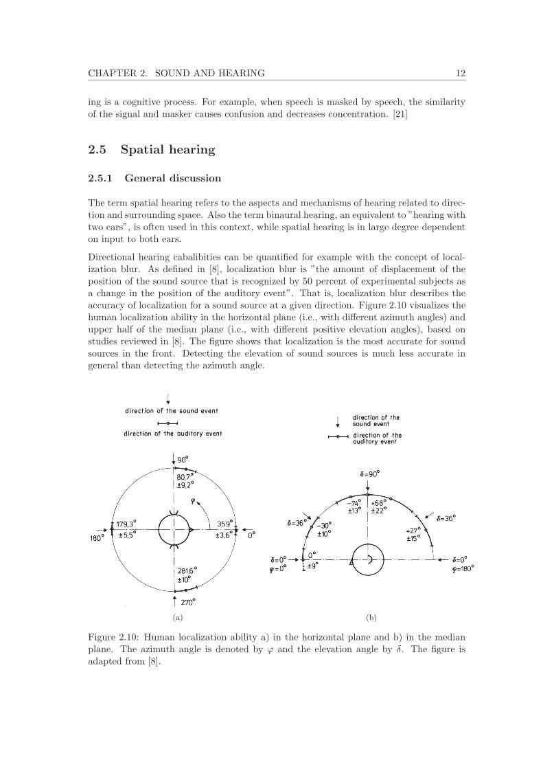
Directional hearing cabalibities can be quantified for example with the concept of local-ization blur. As defined in [8], localization blur is ”the amount of displacement of theposition of the sound source that is recognized by 50 percent of experimental subjects asa change in the position of the auditory event”. That is, localization blur describes theaccuracy of localization for a sound source at a given direction. Figure 2.10 visualizes thehuman localization ability in the horizontal plane (i.e., with different azimuth angles) andupper half of the median plane (i.e., with different positive elevation angles), based onstudies reviewed in [8]. The figure shows that localization is the most accurate for soundsources in the front. Detecting the elevation of sound sources is much less accurate ingeneral than detecting the azimuth angle.
(a) (b)
Figure 2.10: Human localization ability a) in the horizontal plane and b) in the medianplane. The azimuth angle is denoted by ϕ and the elevation angle by δ. The figure isadapted from [8].
CHAPTER 2. SOUND AND HEARING 13
For the following sections, a few terms are elucidated. The term monaural or monoticrefers to listening with only one ear, while in binaural condition both ears are stimulated.Binaural listening condition can be diotic or dichotic. In diotic condition, both ears arestimulated with identical signal, while in dichotic condition the signals are different. Unlikein a sound field, in headphone listening sound sources are generally perceived to be insideor nearby the head and therefore it is relevant only to consider the lateral position of thesound sources in the axis of the ears [8]. Thus, as in a sound field localization is discussed,in headphone listening the relevant term to use is lateralization [8].
2.5.2 Binaural localization cues
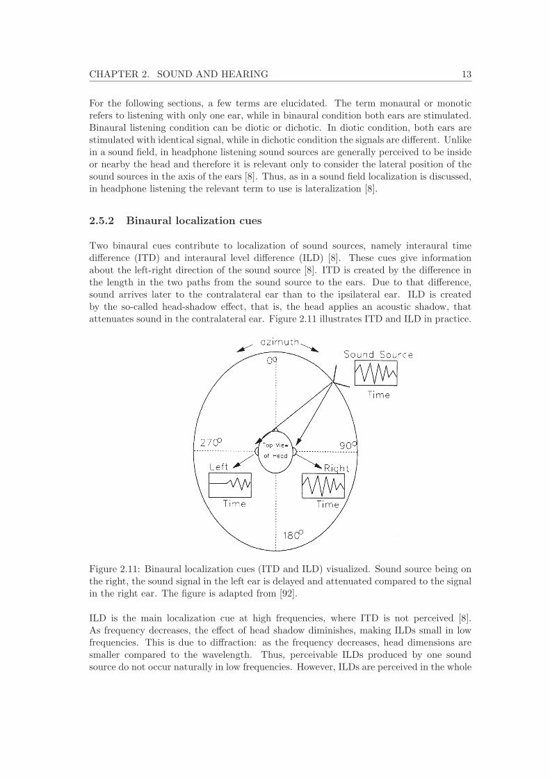
Two binaural cues contribute to localization of sound sources, namely interaural timedifference (ITD) and interaural level difference (ILD) [8]. These cues give informationabout the left-right direction of the sound source [8]. ITD is created by the difference inthe length in the two paths from the sound source to the ears. Due to that difference,sound arrives later to the contralateral ear than to the ipsilateral ear. ILD is createdby the so-called head-shadow effect, that is, the head applies an acoustic shadow, thatattenuates sound in the contralateral ear. Figure 2.11 illustrates ITD and ILD in practice.
Figure 2.11: Binaural localization cues (ITD and ILD) visualized. Sound source being onthe right, the sound signal in the left ear is delayed and attenuated compared to the signalin the right ear. The figure is adapted from [92].
ILD is the main localization cue at high frequencies, where ITD is not perceived [8].As frequency decreases, the effect of head shadow diminishes, making ILDs small in lowfrequencies. This is due to diffraction: as the frequency decreases, head dimensions aresmaller compared to the wavelength. Thus, perceivable ILDs produced by one soundsource do not occur naturally in low frequencies. However, ILDs are perceived in the whole
CHAPTER 2. SOUND AND HEARING 14
frequency range of hearing and thus, for example in headphone listening, it is possible toproduce perceivable ILDs also in low frequencies.
ITD is the main localization cue in low frequencies. It is also called interaural phasedifference (IPD), for in the case of continuous signals time differences translate into phasedifferences. Experiments with pure tones have revealed that the ability to localize soundsources with ITD decreases rapidly after 800 Hz, and above approximately 1.6 kHz thecue is ineffective. [8]
The diminishing perception of ITD by increasing frequency can be understood by a prac-tical example utilizing Equation 2.2. Considering an approximate distance between theears being around 17 cm, this is roughly the maximum difference in length in the twopaths from the sound source to the ears. Thus, the maximum natural ITD is around 0.5ms. This distance corresponds roughly to a half wavelength (maximum phase difference)of a one-kilohertz wave. Thus, at frequencies over 1 kHz, IPD can be in between half andone full wavelength. In this case, the cue is confusing: the IPD can be interpreted in twoways depending on which of the signals in ears is considered leading and which lagging intime. Respectively, above 2 kHz, IPD can several cycles, making the analysis even moreambiguous.
Further studies have been made with a high-frequency carrier signal, for example narrowband noise modulated by a low-frequency envelope. Above 1.6 kHz, the auditory systemcannot decode the phase differences of the ”fine structure” of the carrier, but an ITDapplied to the envelope of the signal is perceived. Envelope-ITDs are to some extentdetected also under 1.6 kHz, depending on the shape of the envelope. Therefore, thecue produced by carrier and envelope ITDs can be in conflict, resulting in two spatiallyseparated auditory events. [8]
2.5.3 Monaural localization cues
Monaural cues, also referred as spectral cues, are generated by the complex, individualshapes of the pinna, head and upper torso. These form a linear filter, the characteristicsof which depend on the direction and distance of the sound source. Mechanisms of thisfiltering include reflection, diffraction, dispersion, interference, resonance, and shadowing.Thus, spatial information of the sound scene is coded to temporal and spectral cues of thesound signal reaching the tympanic membrane. [8]
Considering the shape of the pinna, the direction-dependent filtering is obvious. Especiallythe response for sound sources in the back and front differ substantially. Shoulders, inaddition to pinna, create a difference to the responses for sources with different elevation.This is essential for the human localization ability, while the use of binaural cues is bymuch restricted to the lateral position of the sound source. Indeed, ITD and ILD cues areapproximately constant in a so-called cone of confusion [91], that can be visualized as acircle formed by the bottom of a cone, the apex of which is pointing to the auditory canal.Without spectral cues, front-back and up-down confusion occurs, while the interauralcues are identical in multiple locations. This means, for example, that a source in frontalhemisphere can be confused to be at the symmetrical location at the rear hemisphere.
CHAPTER 2. SOUND AND HEARING 15
2.5.4 Additional factors on localization
Sound source localization is a process with many factors involved. In addition to thecues mentioned in Sections 2.5.2 and 2.5.3, a few other mechanisms are present. First,rotating one’s head alters the monaural and binaural cues. This is utilized more or lessconsciously to fine-tune localization and to solve confusing situations. For example front-back-confusion is solved with head rotation, while the cues produced by sources in thefrontal and rear hemisphere change differently when head is moved. Second, what isseen while hearing, contributes on the sound source localization. For example, when avisual cue is present, the auditory event may be settled at that location, although the realsound source is elsewhere. A visual cue may also externalize a sound source in headphonelistening. Studies on motional and visual theories are reviewed for example in [8].
Localization provides information on the source direction regardless of the indirect soundpresent in enclosed spaces. This is due to precedence effect [92]. That is, sound is localizedbased on the first wavefront (i.e., the direct sound), and the directional information carriedby the early reflections is discarded. Precedence effect occurs, when the time differenceof the signals is over 1–1.5 ms but under 30–40 ms [40]. For two sound sources with timedifferences under 1–1.5 ms, the sources merge to one auditory event, which is localizedsomewhere between the two directions. For time differences over 30–40 ms, the delayedsignal distinguishes as an echo [40].
2.5.5 Binaural advantages in communication
Having two ears not only enables sound source localization, but also contributes to theability to segregate sound sources and to direct attention to one target source. This iscrucial in communication situations with background noise, for example in a cocktail party,where one is trying to understand one talker, although many people are speaking at thesame time. Indeed, listening in this kind of situations is much easier with two ears. Thisis called the cocktail party effect [13], the basis of which is on binaural hearing. Theadvantages of binaural hearing and the phenomena contributing to cocktail party effectare discussed in the following.
Compared to listening with one ear, there are three main advantages in binaural hearing.First, often either of the ears is closer to the talker and has thus a better SNR due tohead shadow. Second, binaural cues allow the speech and noise to be processed separately,further unmasking the speech. This is called the squelch effect. Finally, the total loudnessis increased, when two ears receive sound. This is called the binaural summation effect.[49]
The cocktail-party effect is partly explained by the concept of binaural masking: thethreshold of detecting a signal in the presence of a masker depends on the listening con-dition. Fundamentally, the thresholds are the same in monotic and diodic conditions, butlower in a dichotic condition. That is, the masking effect is less effective when signal andnoise have different interaural configuration. Binaural masking can be quantified withthe term masking level difference (MLD). MLD is defined as the difference between thethreshold of detecting masked signal in a certain condition compared to monotic condition.MLD can be up to 15 dB, in case of 1000 Hz sinusoid signal masked with white noise. This
CHAPTER 2. SOUND AND HEARING 16
suggests, that if one ear is occluded at a cocktail party, the speech intelligibility decreasesnotably. However, MLD decreases notably when frequency increases. [92]
A term related to MLD is spatial release from masking (SRM). SRM describes the bene-ficial change in masked hearing threshold when the signal and masker are spatially sepa-rated, compared to them being in the same location (i.e., co-located) [50]. Additionally,when speech intelligibility is used as the measured quantity when assessing masking leveldifference, the terms monaural intelligibility level difference (MILD) and binaural intelli-gibility level difference (BILD) are used [8].
A study by Marrone et al. [50] exemplifies the concept of binaural masking. In the study,SRM was measured using three loudspeakers, each with their own one-talker speech signal.The target talker was positioned in the front and the two others were symmetrically placedon the sides, with varying azimuth. Due to the signals used, there was both energetic andinformational masking involved. The SRM was measured to be 8 dB when the separationbetween signal and masker was ±15◦. The maximum SRM of 12 dB was reached after±45◦ and no substantial change was noticed between angles ±45–90◦. When one ear wasoccluded, this effect was gone.
Another conclusion in the study by Marrone et al. [50] was that informational maskinghad a greater effect in a co-located condition than in a spatially separated condition.This was noticed when SRMs were measured with the masker signals time-reversed, whicheliminated the informational masking effect of the speech. Time-reversing increased theperformance (i.e., lowered the masked threshold) by 12 dB in the co-located, but only5 dB in the spatially segregated condition. This means that the SRM is higher wheninformational masking occurs. As the spatial segregation had already applied a largeimprovement in the masked threshold, eliminating the informational masking did notfurther improve the situation as much as it was improved in the co-located condition.
Furthermore, in the SRM-tests of Marrone et al. [50], the SRM decreased when reverbera-tion was added to the test booth. This is logical: as reverberation increases the diffusenessof the sound field, the effective spatial separation of such sources decreases. Similar resultswere achieved in [72], in which the benefit of hearing aid with directional microphone wasstudied: it was noted that increased reverberation decreased the directional benefit andperformance.
The effect of spatial separation of speech and background noise signal to the speech intelli-gibility was studied by Rychtarikova et al. [74]. In that study, significant differences werenoticed between the speech intelligibility measured in cases S0N0, S0N90, and S0N180 inanechoic conditions3. The best intelligibility was generally in the case S0N90, and the sec-ond best in the case S0N180. Poorest performance was recorded in the case S0N0, wherethere was no spatial separation. The results were explained with binaural filtering in thecase S0N90 and spectral filtering in the case S0N180. However, when the same test wasconducted in a reverberant room, the differences between the three cases were minimal.[74]
3The notation SxNy means that the signal and noise are presented in azimuths x and y, respectively.

Chapter 3
Techniques for spatial audio
In the previous chapter, the perceivable spatial attributes of sound were discussed. Thischapter briefly discusses techniques for capturing and reproducing such attributes. Acursory overview of spatial audio reproduction techniques is given in Section 3.1. Oneof such techniques, Directional Audio Coding, is put more emphasis on and describedin Section 3.2. Elaborated discussion of these topics are not in the scope of this thesis.Thereby, interested reader is encouraged to explore the references provided in this chapter.
3.1 Approaches to spatial audio reproduction
3.1.1 Spatial audio with loudspeakers
One approach to reproduce spatial audio is Wave Field Synthesis (WFS), in which thephysical sound field is targeted to be reconstructed [7]. It is based on Huygens’ principle1.In WFS, loudspeakers are arranged in an array and each loudspeaker is fed separately withdedicated delay. Loudspeakers must be closely spaced and carefully calibrated. Thus, avery high number of loudspeakers is needed.
Another technique is Ambisonics [26]. In Ambisonics, the sound field in single positionis captured with an array of directional microphones and reproduction is done with aloudspeaker array. In first-order Ambisonics, sound is captured in B-format, which con-sists of four microphone channels. Higher-order approaches utilize more channels. Withambisonics, high-quality reproduction is achieved in the center of the loudspeaker array,in a so-called sweet spot. However, this sweet spot is small: in first-order Ambisonics, thesweet spot is larger than a human head only in frequencies under 700 Hz [81]. Problemsarise when listening outside of the sweet spot. Namely, the loudspeaker signals are coher-ent, resulting in comb-filter effects outside the sweet spot. Furthermore, due to precedenceeffect, sound event is localized to the nearest loudspeakers.
Currently, in consumer sector, spatial audio reproduction is mainly restricted to standard-ized loudspeaker setups and their dedicated audio formats. Perhaps the most commonof these is the 5.1 system, consisting of five mid/high-frequency loudspeakers and one
1Huygens’ principle states that any wavefront can be constructed as a superposition of elementarysphere waves [93].
17

CHAPTER 3. TECHNIQUES FOR SPATIAL AUDIO 18
subwoofer. Figure 3.1 shows the ITU-R BS.775-1 [36] specification for the loudspeakerplacement in the 5.1 system. For this kind of standardized system, audio content can becreated with various recording and mixing techniques. Generally, the idea is to generatean enveloping auditory event with the surround loudspeakers. Several variations of thisstandard with different number of loudspeakers exists, which usually are based on the 5.1arrangement. The naming logic is the same: first the number of loudspeakers and thenthe number of subwoofers separated with a point. Thus, a conventional stereo setup canbe called a 2.0 system.
Figure 3.1: The 5.1 standard specified in ITU-R BS.775-1. Letters L, C, R, LS and RS referto loudspeakers labeled left, center, right, left surround, and right surround, respectively.The subwoofer location is not specified. The figure is adopted from [87].
3.1.2 Spatial audio with headphones
Besides loudspeakers, also headphones can be used in spatial audio. In this case, however,including the monaural localization cues to the headphone signals is required in order toreproduce the sense of space. One approach for this is to do binaural recordings using twomicrophones placed in the ears of an artificial or real head and reproducing these signalswith headphones. Thus, localization cues are naturally coded into the headphone signals.However, when listening to binaural recordings, the sound scene moves as the listener headmoves and this decreases the localization accuracy and realism. Furthermore, individualrecordings are needed for accurate reproduction.
Another approach is to use Head-Related Transfer Function (HRTF) techniques. HRTFsdefine how the sound is altered due to the head and shoulders of the listener for given sound
CHAPTER 3. TECHNIQUES FOR SPATIAL AUDIO 19
source directions. These functions can be used to produce localization cues in headphonelistening [91]. HRTFs are measured using binaural recording methods; generic HRTFscan be measured for example with an artificial head. As well as body shapes, HRTFs areindividual. It has been shown for example in [91] that localization performance decreasesif non-individual HRTFs are used. Often the problem with non-individual HRTFs is thatsound sources are localized inside the head. Using HRTFs is advantageous compared tobinaural recordings, because HRTFs can be easily modified and convolved with audiomaterial. For instance, HRTFs can be controlled in real time by listener head movementto enhance the realisticity of the reproduction. Head-tracking is advantageous as it helpsto externalize the sound events, that is, to localize the sound sources outside the headinstead of inside.
3.2 Directional Audio Coding (DirAC)
3.2.1 The idea in brief
Directional Audio Coding (DirAC) [68] is a spatial sound reproduction method for ar-bitrary loudspeaker setups. Rather than reconstructing or modeling the physical soundfield, DirAC aims at preserving the perceptual attributes of the recorded sound field.Consequently, several assumptions are made of the relation between the physical aspectsof sound and the perception they produce. First, the spatial auditory image perceivedby a human listener is assumed to be determined by three factors: direction of arrival,diffuseness and spectrum of sound. Thus, if these factors are measured in one locationand with the temporal and spectral resolution of human hearing, the spatial auditory im-age would be reproducible. Second, ITD, ILD, and monaural cues are assumed to definethe perceived direction of arrival, whereas interaural coherence is assumed to define thediffuseness of sound. Third, the perceived timbre is assumed to depend on the monauralspectrum as well as ITD, ILD and interaural coherence. Finally, it is assumed that withinone critical band and one time instant, the auditory system cannot decode cues from twowavefronts coming from different directions. [68]
Based on the assumptions mentioned above, DirAC analysis and synthesis are implementedas follows. In the analysis, to mimic the spectral resolution of the human auditory system,microphone signals are divided to frequency bands where processing is done separately.Direction of arrival, diffuseness, and timbre of sound are then analyzed with the temporalaccuracy relevant to the auditory system in each frequency band. In the synthesis, thesignal is dynamically divided to diffuse- and nondiffuse streams which are reproduced in adifferent manner. The diffuse stream is reproduced by all loudspeakers in use, aiming atsurrounding perception of sound with no prominent direction of arrival. The nondiffusestream is reproduced with Vector Base Amplitude Panning (VBAP) [63] aiming to producepoint-like virtual sound sources. [68]
DirAC is based on a technique called Spatial Impulse Response Rendering (SIRR), whichis described in [53]. The assumptions reviewed above are common with DirAC and SIRR.In a sense, SIRR is like DirAC for impulses. That is, in SIRR, signal content is known tobe an impulse and the recording has been made with one source.
In addition to high quality spatial audio reproduction (e.g., in [85]), DirAC has been
CHAPTER 3. TECHNIQUES FOR SPATIAL AUDIO 20
applied to hearing aids [2] and teleconferencing purposes [1]. SIRR on its own enables forexample room acoustics reproduction [69].
3.2.2 A-format and B-format input signals
Several implementations of DirAC exist, using either A-format or B-format input signals.A-format is the output format from a microphone array consisting of four cardioid orsubcardioid microphone capsules on the faces of a tetrahedron, such as the Soundfieldmicrophone [25]. The A-format capsule signals are denoted LF, LB, RF, RB, which referto left-front, left-back, right-front, and right-back. An A-format signal can be convertedto B-format by linear combination of the A-format microphone capsule signals. B-formatconsists of four signals: one omnidirectional signal (W) and three figure-of-eight signalspointing forward, left, and up (X, Y, and Z) [26]. B-format signals are used also in first-order Ambisonics [26]. Furthermore, from B-format signal, virtual microphone signalspointing to any direction can be formed by a linear combination.
3.2.3 Limitations and drawbacks
As all spatial audio techniques, DirAC has its limitations and drawbacks. One limitationarises from the non-idealities of VBAP. Virtual sound sources generated with VBAP aresharp and localized accurately when they are positioned near the median plane and gen-erated by a loudspeaker pair or triplet symmetrical to the median plane [66]. However,localization of virtual sources positioned further from the median plane is a bit biased to-wards the median plane [67]. Also, depending on the source direction, the virtual sourcesare not always as point-like as real sources [64]. Furthermore, coloration of the virtualsources occurs: for a virtual source formed by two loudspeakers, comb filtering occurswith the first dip in the magnitude response located approximately at 1–2 kHz. [65]. Thiseffect is dependent on the number of loudspeakers used and their positioning [65]. Also,reverberation in the listening room decreases the audibility of the effect [65].
Another issue arises from the psychoacoustic assumptions of DirAC. The validity of theseassumptions has not been proved with hearing-impaired listeners or hearing instrumentusers.
Also, the estimates of DirAC parameters are distorted by the non-idealities of the micro-phone used. For example, the four microphone capsules of a Soundfield microphone arenot coincident, resulting in overestimated diffuseness in high frequencies. However, thisproblem was addressed for instance in [61], where a DirAC implementation using A-formatinput signals was described. In the A-format version, the estimation of diffuseness and di-rection of arrival is correct up to higher frequencies, compared to earlier implementationswith B-format input signals [61].

Chapter 4
Overview of technical audiology
This chapter briefly introduces the key concepts of technical audiology in the scope ofinterest of this thesis, providing the essential prerequisites for the following chapters. Sec-tion 4.1 classifies different hearing disorders and discusses how they affect to hearing, themain focus being on sensorineural hearing loss. Section 4.2 discusses hearing instruments.An overall glance to hearing diagnostics is given in Section 4.3. Hearing diagnostics con-ducted with loudspeakers (i.e., sound-field audiometry) is a key topic in this thesis and isthus discussed separately and in more detail in Section 4.4.
4.1 Hearing disorders
4.1.1 Types of hearing disorders
A hearing disorder is a structural or functional impairment of the auditory system. Mostimportantly, a hearing disorder degrades communication abilities. Even a slight hearingdisorder can affect the perception of music. A more severe hearing disorder complicatesthe ability to react to sonic signals in the environment. Moreover, sufficient hearing in theearly age is of paramount importance to ensure proper linguistic development. [40]
Medically, hearing disorders divide into two main types: conductive and sensorineural.Conductive disorders are due to abnormalities in the outer and middle ear whereas sen-sorineural disorders are due to abnormalities of the inner ear or the auditory nerve. Sen-sorineural disorders can be further divided in cochlear (i.e., sensorial) and retrocochlear(i.e., neural) disorders. Finally, although not discussed in this thesis, there are centraldisorders, which relate to disfunction in the central auditory nervous system. [38, 40, 51]
Hearing disorders result in varying symptoms. The most common symptom is degradationof the sensitivity of hearing (i.e., hearing loss), which can be conductive or sensorineu-ral. In addition to hearing loss, sensorineural disorders include tinnitus and hyperacusis.The following subsections discuss the origin, symptoms and consequences of the hearingdisorders mentioned above.
21

CHAPTER 4. OVERVIEW OF TECHNICAL AUDIOLOGY 22
4.1.2 Conductive hearing loss
Conductive hearing losses are caused by abnormalities in the conductive path in auditorysystem, that is, the outer and middle ear. Outer ear abnormalities can be such as occlusionof the auditory canal due to ear wax, foreign object, tumor, or deformation. Also, thetympanic membrane may become perforated, thickened, or scarred due to mechanicaltrauma or infection in the middle ear, in some cases leading to hearing loss. [51]
There are several middle ear abnormalities that may cause hearing loss. Infection of themiddle-ear cavity is the most common of these, especially in children. Another cause isMucous otitis media, which is caused by mucoid secretions that have ended up into middleear via eustachian tube. Also, malfunction of the eustachian tube may cause air pressuredifference between middle and outer ear, displacing the tympanic membrane and possiblycausing mild hearing loss. [51]
The hearing losses mentioned above usually apply equal amount of attenuation acrossfrequencies. However, some middle ear abnormalities cause hearing loss with non-flatspectrum. Significant negative pressure in the middle ear can cause serous effusion, whichmeans fluid accumulation to the middle ear. This increases the mass of the middle ear, andtherefore the resulting hearing loss is more severe in high frequencies. In adults, the mostcommon middle-ear related cause for hearing loss is otosclerosis. It is a progressive disorderwhere a new growth of spongy bone stiffens the movement of the auditory ossicles, oftenpartially fixing the stapes to the oval window. This attenuates the vibration transmittedby the middle ear. The hearing loss caused by otosclerosis is either flat in frequency orsomewhat more severe at low frequencies. [51]
4.1.3 Sensorineural hearing loss
Sensorineural hearing loss is often caused by excessive exposure to noise. Noise-inducedhearing loss is caused by a single brief or repeated exposures to high-level sound. The termacoustic trauma is commonly used to describe a brief exposure to high level sound, forexample a gunshot. The hearing loss caused by a single acoustic trauma can be followed bycomplete or partial recovery, although it can result in permanent impairment. Repeatingtemporary impairments usually result in permanent hearing loss. [40, 51]
In the auditory system, hair cells are the most vulnerable part to acoustic overstimulation.Although a really high level noise can damage also other parts of the ear, such as thetympanic membrane, much lower levels are adequate to damage hair cells. Hair cellscan recover from slight damages, but if severely damaged, hair cells do not recover norare new cells generated. The degree of noise-induced hearing loss depends on the energyreceived by ear, that is, the combination of sound level and exposure duration. After suchdamage, the metabolic activity in the exerted hair cell contributes on the permanency ofthe impairment. [92]
Besides noise, there are several other causes for sensorineural hearing loss. The most usualof them is presbycusis, the aging-related hearing loss. On the other hand, sensorineuralhearing loss can be inborn. Furthermore, damages of the inner ear can be caused by aserious head trauma or cancer in the auditory nerve. Some drugs and other substancesare ototoxic, meaning that they damage the inner ear. Otosclerosis, discussed in Section
CHAPTER 4. OVERVIEW OF TECHNICAL AUDIOLOGY 23
4.1.2, can also involve the cochlea and thereby result in sensorineural hearing loss. Suddenidiopathic hearing loss may occur by viral or vascular origin. Finally, Meniere disease cancause sudden hearing loss. [51]
Difficulty in speech understanding, especially in the presence of background noise, is acommon problem among people with sensorineural hearing loss [10, 56, 62]. Indeed, studieshave shown degraded speech intelligibility in noise among individuals with sensorineuralhearing loss compared to normally-hearing individuals [56]. It appears that people withsensorineural hearing loss are less able to benefit from the temporal and spectral dips inspeech [56]. This reflects a disfunction of the active mechanism in the cochlea, that is, themechanism providing nonlinear characteristics to hearing, such as frequency selectivityand compression [56]. Damage in the outer hair cells inhibits the mechanism to functionproperly [56]. In the following, the aspects of sensorineural hearing loss contributing tospeech intelligibility are discussed.
Hearing threshold shift
Hearing threshold shift is the main consequence of sensorineural hearing loss. It has anobvious effect on speech intelligibility: if a part of the information remains inaudible,speech discrimination is degraded. Depending on the cause, a hearing loss can be equallyintense across frequencies or more intense in some frequency range. This contributes tohow much the hearing loss affects communication abilities. For instance, discriminationof the fundamental frequency of speech is not as important as hearing the consonants,located in higher frequencies. [38]
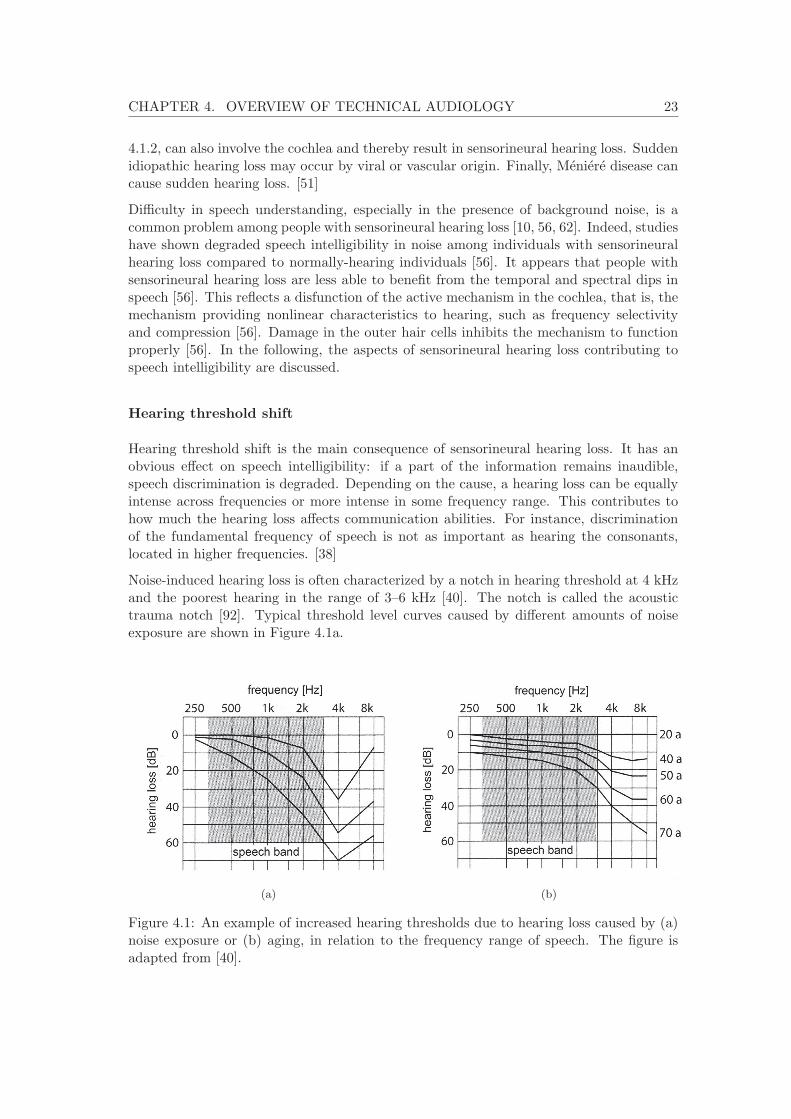
Noise-induced hearing loss is often characterized by a notch in hearing threshold at 4 kHzand the poorest hearing in the range of 3–6 kHz [40]. The notch is called the acoustictrauma notch [92]. Typical threshold level curves caused by different amounts of noiseexposure are shown in Figure 4.1a.
(a) (b)
Figure 4.1: An example of increased hearing thresholds due to hearing loss caused by (a)noise exposure or (b) aging, in relation to the frequency range of speech. The figure isadapted from [40].
CHAPTER 4. OVERVIEW OF TECHNICAL AUDIOLOGY 24
It is important to notice that a mild noise-induced hearing loss does not typically extendto the speech band. However, a severe noise-induced hearing loss affects also the speechband, and thus degrades communication abilities. On the other hand, presbycusis usuallybegins from the highest frequencies and slowly progresses to lower frequencies with age[92]. Figure 4.1b shows hearing threshold curves typical to patients with presbycusis.
Decreased frequency resolution of hearing
Damaging of the outer hair cells decreases the frequency resolution of hearing [38, 56].This can be understood with the tuning curves, presented in Figure 2.6. Namely, when thehearing threshold increases, the sharp tip of the tuning curve flattens, making individualcurves wider [56]. This makes the hair cell less frequency-selective.
Although the decrease in the frequency resolution itself does degrade the speech discrimina-tion abilities [38], more importantly it affects the masking effect. Namely, as the frequencyselectivity decreases, critical bandwidth broadens. Thus, more energy is summed to onecritical band and this intensifies the masking effect [38]. In other words, the maskingthreshold curves shown in Figure 2.9 broaden and the effect of a mask tone spreads towider frequency area, thus making the masking effect more effective [62].
The effective increase of masking due to sensorineural hearing loss can be up to 10–12 dB[38]. Increased masking effect affects significantly to the speech discrimination abilities inthe present of background noise [38]. Therefore, even though speech was above hearingthreshold, a person with sensorineural hearing loss generally needs better SNR to recognizespeech.
Decreased dynamic range of hearing
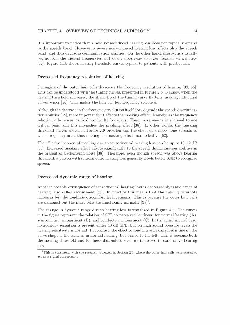
Another notable consequence of sensorineural hearing loss is decreased dynamic range ofhearing, also called recruitment [83]. In practice this means that the hearing thresholdincreases but the loudness discomfort level remains. This is because the outer hair cellsare damaged but the inner cells are functioning normally [38]1.
The change in dynamic range due to hearing loss is visualized in Figure 4.2. The curvesin the figure represent the relation of SPL to perceived loudness, for normal hearing (A),sensorineural impairment (B), and conductive impairment (C). In the sensorineural case,no auditory sensation is present under 40 dB SPL, but on high sound pressure levels thehearing sensitivity is normal. In contrast, the effect of conductive hearing loss is linear: thecurve shape is the same as in normal hearing, but biased to the left. This is because boththe hearing threshold and loudness discomfort level are increased in conductive hearingloss.
1This is consistent with the research reviewed in Section 2.3, where the outer hair cells were stated toact as a signal compressor.

CHAPTER 4. OVERVIEW OF TECHNICAL AUDIOLOGY 25
Figure 4.2: Changes in the dynamic range of hearing due to sensorineural hearing loss.The curves show the relation of sound pressure level and the perceived loudness. Curve Ais for normal hearing, B for sensorineural hearing loss and C for conductive hearing loss.The figure is adapted from [83].
Additional aspects
Additionally, a reduction of temporal resolution, intensity resolution and temporal inte-gration has also been reported to result from cochlear damage [56]. Moreover, distortedpitch perception and reduced frequency discrimination has been reported [56].
In a case of a severe unilateral or considerably asymmetric hearing loss, the binauraladvantages of hearing are obviously degraded or lost. First of all, this causes a decreasein localization abilities [38, 56]. Second, this causes a degradation in hearing abilitiesin noise due to a decreased masking level difference [56]. That is, the benefit from thespatial separation of signal and noise is decreased [56]. Moreover, for a normal hearingindividual, comparing the signals at the two ears, or using the ear with the better SNR,is advantageous when hearing in the presence of noise [56].
4.1.4 Tinnitus and hyperacusis
In addition to hearing loss, several other sensorineural hearing disorders exist. These aresuch as tinnitus and hyperacusis. Both of these are most commonly caused by excessivenoise exposure.
CHAPTER 4. OVERVIEW OF TECHNICAL AUDIOLOGY 26
Tinnitus means some kind of auditory event without any external sound event. This”ringing in the ears” can be continuous or occasional. According to [38], over half of thehearing losses are accompanied by tinnitus. However, tinnitus occurs also with individualswith normal hearing thresholds [38]. In some cases, tinnitus is related to a hearing impair-ment that has not yet realized as a threshold shift [38]. Among the tinnitus patients withacoustic trauma notch, the tinnitus tone can be often matched to the frequency range of3000–6000 Hz [51]. However, the perceived tinnitus tones vary a lot individually. Besidesnoise exposure, temporary tinnitus can be due to vertigo, nausea, Meniere disease andbloodstream-related problems [51].
The literature contains several explanations for the mechanism of noise-induced tinnitus.According to [38], the damaged part of the basilar membrane stimulates the auditory nervecontinuously, causing changes to its spontaneous action. The central auditory nervoussystem does not inhibit this changed spontaneous action [38]. Actually, it may evenamplify this, because the sensitivity of the nerve pathways may be dependent on theexternal sound scene [38]. Hence, the spontaneous action and thereby also the loudness oftinnitus may be increased in quiet environments [38]. On the other hand, several studieshave suggested the mechanism of tinnitus to be retrocochlear. For instance, in [6] evidencewas shown for tinnitus to be an auditory phantom perception generated in the central levelof the auditory nervous system.
Hyperacusis means a decreased loudness discomfort level. While recruitment is fundamen-tally always preceded by hearing loss, hyperacusis does not necessarily relate to hearingloss. Actually, most individuals with hyperacusis have normal hearing thresholds. How-ever, in hyperacusis the dynamic range of hearing is decreased as the tolerance of loudnessis lower. Hyperacusis if often preceded by acoustic trauma and accompanied by tinnitus.[51]
4.2 Hearing instruments
4.2.1 Hearing aid
A hearing aid is like a miniature public address system with signal processing. It amplifiesand processes sound to adequately compensate the effect of hearing loss. Different typesof hearing aids are shown in Figure 4.3. The small hearing aids inserted into the ear orauditory canal (Figures 4.3a and 4.3b) are advantageous, because they allow the pinna-related directional cues and are cosmetically indistinguishable. The increase in availableprocessing power has enabled the use of more complicated algorithms and more compactsize of the device.
The simplest possible hearing aid would be a combination of a microphone near the ear, alinear amplifier with constant gain thorough the audible frequency range, and a miniatureloudspeaker providing the amplified sound to the auditory canal. This may be enoughto compensate a mild conductive hearing loss with flat spectrum, but not adequate withcases involving frequency- and intensity-dependent attenuation. Thus, modern hearingaids include frequency-dependent amplification, compression and other signal processing,tuned individually for each user. These features are specified in the following.
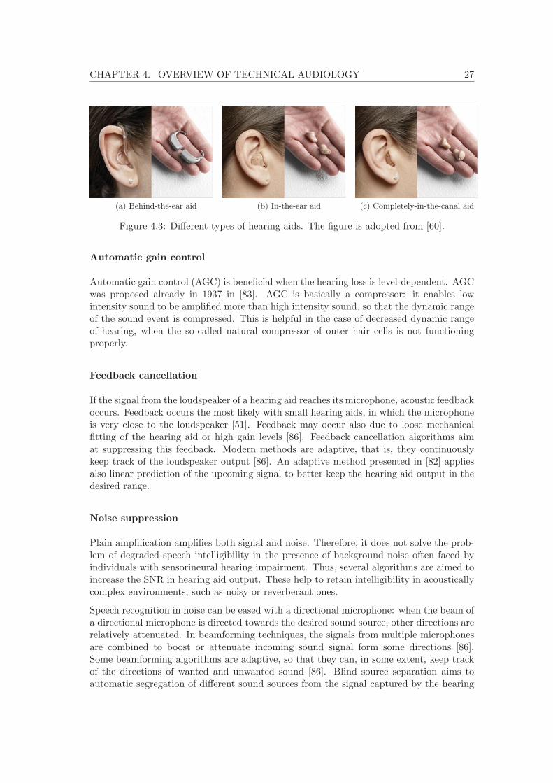
CHAPTER 4. OVERVIEW OF TECHNICAL AUDIOLOGY 27
(a) Behind-the-ear aid (b) In-the-ear aid (c) Completely-in-the-canal aid
Figure 4.3: Different types of hearing aids. The figure is adopted from [60].
Automatic gain control
Automatic gain control (AGC) is beneficial when the hearing loss is level-dependent. AGCwas proposed already in 1937 in [83]. AGC is basically a compressor: it enables lowintensity sound to be amplified more than high intensity sound, so that the dynamic rangeof the sound event is compressed. This is helpful in the case of decreased dynamic rangeof hearing, when the so-called natural compressor of outer hair cells is not functioningproperly.
Feedback cancellation
If the signal from the loudspeaker of a hearing aid reaches its microphone, acoustic feedbackoccurs. Feedback occurs the most likely with small hearing aids, in which the microphoneis very close to the loudspeaker [51]. Feedback may occur also due to loose mechanicalfitting of the hearing aid or high gain levels [86]. Feedback cancellation algorithms aimat suppressing this feedback. Modern methods are adaptive, that is, they continuouslykeep track of the loudspeaker output [86]. An adaptive method presented in [82] appliesalso linear prediction of the upcoming signal to better keep the hearing aid output in thedesired range.
Noise suppression
Plain amplification amplifies both signal and noise. Therefore, it does not solve the prob-lem of degraded speech intelligibility in the presence of background noise often faced byindividuals with sensorineural hearing impairment. Thus, several algorithms are aimed toincrease the SNR in hearing aid output. These help to retain intelligibility in acousticallycomplex environments, such as noisy or reverberant ones.
Speech recognition in noise can be eased with a directional microphone: when the beam ofa directional microphone is directed towards the desired sound source, other directions arerelatively attenuated. In beamforming techniques, the signals from multiple microphonesare combined to boost or attenuate incoming sound signal form some directions [86].Some beamforming algorithms are adaptive, so that they can, in some extent, keep trackof the directions of wanted and unwanted sound [86]. Blind source separation aims toautomatic segregation of different sound sources from the signal captured by the hearing

CHAPTER 4. OVERVIEW OF TECHNICAL AUDIOLOGY 28
aid microphone [86]. Beamforming and blind source separation are helpful in the presenceof directional noise sources for they can be effectively attenuated. The increased speechintelligibility due to use of a directional hearing aid microphone was studied for examplein [15]. The study discovered, for example, that with omnidirectional microphone, a 5dB better SNR was needed to achieve the same level of speech intelligibility compared tosupercardioid [15].
Noise suppression can also be done with a single-microphone devices. Single-channel noisereduction systems use the temporal, spectral and statistical information of the incomingsound and are thus the most effective against stationary and diffuse noise. [62]
Binaural processing
Even if hearing aids were used in both ears, the signal processing in the two aids are notgenerally interrelated [88]. Consequently, ILD-cues are distorted by the unsynchronizedgain processing in the two aids [4]. Furthermore, ITD-cues are often distorted by themonaural noise suppressing algorithms [44].
The following terminology is often used to discriminate between linked and non-linkedprocessing. Bilateral hearing aid refers to using of hearing aids in both ears. Binauralhearing aid instead includes that the processing in the two aids is linked to some extent.
With binaurally aided hearing, binaural cues could be preserved to some extent [62]. Thiswould enhance hearing-in-noise performance, due to detection of spatial separation ofsound sources. Preserving of ILD cues in aided hearing was discussed in [4]. In that study,SRT-scores were measured with bilaterally synchronized and unsynchronized gain process-ing using spatially segregated signal and noise sources [4]. Somewhat better SRT-scoreswere measured when using bilaterally synchronized hearing aids [4]. Another advantage inbinaural processing is that the coherence of left and right input channels can be analyzedand used to suppress diffuse background noise [86]. Additionally, blind source separationcould be enhanced with binaural processing [62].
4.2.2 Cochlear implant
A cochlear implant is a bionic ear: it is an electronic device that stimulates the auditorynerve with an electrode array inserted in the cochlea. Thus, the whole conductive andsensory path of the auditory system is bypassed. Alike are bypassed the functions providedby the inner ear, such as frequency analysis and compression.
Figure 4.4 shows a schematic of a cochlear implant. First, there are the external parts,usually located behind the pinna: a microphone, a sound processor, and a transmittercoil. The external parts capture sound, encode it to digital format, and transmit it to theimplant. Under the skin, there is a receiver coil and a processor converting the digitalsound to electrical impulses. These pulses are sent to an electrode array inside cochlea.Each electrode represents a given frequency band, and stimulates the respective nervefibers. [14]
The first cochlear implants included only one electrode and were aimed to provide soundawareness. Modern implants have currently up to 22 electrodes, providing more spectral

CHAPTER 4. OVERVIEW OF TECHNICAL AUDIOLOGY 29
Figure 4.4: A schematic of a cochlear implant. The figure is adapted from [84].
information [14]. The results vary depending on the individual: not every patient reachesgood speech recognition, but for some, normal telephone conversation is possible [55].
Although the sound quality in current cochlear implants is not comparable to normalhearing, they can enable adequate hearing in situations where unaided hearing abilitiesare very low and hearing aid would be useless. This would be the case for example in asevere impairment of the conductive path or severe cochlear impairment.
4.2.3 On hearing with hearing instruments
In aided hearing, some of the problems induced by hearing loss may remain and some newones may arise. To begin with, hearing through a hearing instrument has an effect onthe monaural cues. If the microphone is located behind the ear – or generally anywhereelse than in the auditory canal – the spectral cues provided by the pinna are lost. Also,according to [56], the monaural cues are often lost when using hearing aid, because the aidmodifies the spectral content of the sound and does not always amplify frequencies above6 kHz, where the pinna cues are the most prominent. However, some signal processingtechnologies exists that aim to preserve spectral cues [80].
The effect on the binaural cues is more complex. As discussed in Section 2.5, a normally-hearing person relies on ITD in low frequencies frequencies and ILD on higher frequen-cies. The research reported in [23] explored the localization mechanisms used by bilateralcochlear implant users. The study participants seemed to rely mainly on ILD. Little sup-plement was got from ITD cues of the signal envelopes if the test tone was pulsating.Thereby, the localization abilities of the test subjects were quite poor in low frequencies,where ILD cues are not present. In addition, while normally-hearing individuals have two
CHAPTER 4. OVERVIEW OF TECHNICAL AUDIOLOGY 30
cues in use for confusing situations, cochlear implant users must get along mostly withone cue. In the study, this was proposed to be a significant issue especially in situationswith several sound sources or speech in competing noise.
The relative contribution of ILD and ITD cues to bilateral cochlear implant users wasfurther discussed in [3]. The study concluded that ILD is the major cue used by bilateralcochlear implant users. However, the performance with only ITD cues available was betterthan with no cues at all, suggesting that some information about the time differences isanyhow used. The performance with ITD and ILD cues was similar to the performancewith only ILD cues.
Using two hearing instruments instead of one seems to result in better hearing perfor-mance. In [75] it was concluded that binaural cochlear implant users can benefit fromthe same advantages of binaural hearing to speech intelligibility than do normally-hearingindividuals. In [57] the benefit of bilateral cochlear implant to localization and speechdiscrimination in noise was investigated. In that study, 67 % of the patients showed sig-nificant increase in these abilities when a bilateral cochlear implant was inserted, comparedto the use of an unilateral implant [57]. Also in [59] the sound localization among cochlearimplant users was investigated. That study similarly found significant improvement inthe localization accuracy when bilateral implant was used, compared to unilateral implant[59]. In that study, the mean deviation between real azimuth and response was 16.6◦ withbilateral implant and 53.1◦ with unilateral implant [59].
However, even if two hearing instruments were used, ITD cues might be lost due tounsynchronized processing in the right and left side. If the processing in the left andright implant was synchronized, the ITD cues could possibly be preserved and thus thehearing performance would possibly be better.
4.3 Hearing diagnostics
4.3.1 Pure-tone audiometry
In pure-tone audiometry (PTA), hearing thresholds are determined at different frequenciesusing pure tones as test signals. The test procedures in PTA follows an adaptive procedure,defined in standard ISO 8253-1 [32]. Generally, the patient listens in a quiet environmentand gives a signal (e.g., presses a button) each time a sound is heard. The test conductorplays short-duration test tones one at a time, alters the sound level depending on thepatient’s response, and searches the hearing threshold level. This procedure is repeated foreach tested frequency. If the patient has tinnitus or a hearing instrument that suppressespure tones, warble tones can be used as the test signal instead of pure tones [51]. Warbletone is a frequency-modulated pure tone, the frequency of which wobbles rapidly aroundthe tested frequency.
The reference level of normal hearing has been achieved with large-scale measurements ofyoung individuals and is defined in the standard ISO 389 [31]. This curve is called hearinglevel (HL) and a deviation from it due to hearing loss can be denoted in decibels relativeto hearing level (dB HL).
PTA can be done in air or bone conduction. Air conduction measurements are typically
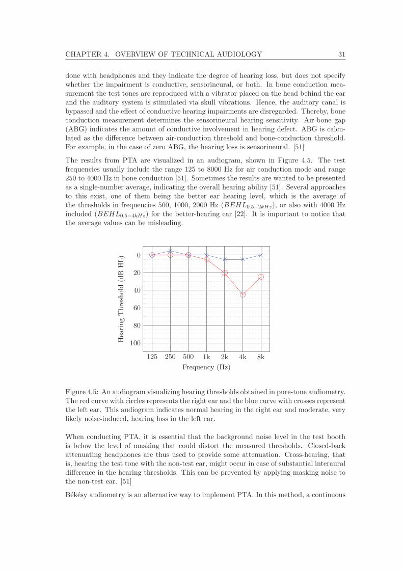
CHAPTER 4. OVERVIEW OF TECHNICAL AUDIOLOGY 31
done with headphones and they indicate the degree of hearing loss, but does not specifywhether the impairment is conductive, sensorineural, or both. In bone conduction mea-surement the test tones are reproduced with a vibrator placed on the head behind the earand the auditory system is stimulated via skull vibrations. Hence, the auditory canal isbypassed and the effect of conductive hearing impairments are disregarded. Thereby, boneconduction measurement determines the sensorineural hearing sensitivity. Air-bone gap(ABG) indicates the amount of conductive involvement in hearing defect. ABG is calcu-lated as the difference between air-conduction threshold and bone-conduction threshold.For example, in the case of zero ABG, the hearing loss is sensorineural. [51]
The results from PTA are visualized in an audiogram, shown in Figure 4.5. The testfrequencies usually include the range 125 to 8000 Hz for air conduction mode and range250 to 4000 Hz in bone conduction [51]. Sometimes the results are wanted to be presentedas a single-number average, indicating the overall hearing ability [51]. Several approachesto this exist, one of them being the better ear hearing level, which is the average ofthe thresholds in frequencies 500, 1000, 2000 Hz (BEHL0.5−2kHz), or also with 4000 Hzincluded (BEHL0.5−4kHz) for the better-hearing ear [22]. It is important to notice thatthe average values can be misleading.
125 250 500 1k 2k 4k 8k
0
20
40
60
80
100
Frequency (Hz)
HearingThreshold
(dB
HL)
Figure 4.5: An audiogram visualizing hearing thresholds obtained in pure-tone audiometry.The red curve with circles represents the right ear and the blue curve with crosses representthe left ear. This audiogram indicates normal hearing in the right ear and moderate, verylikely noise-induced, hearing loss in the left ear.
When conducting PTA, it is essential that the background noise level in the test boothis below the level of masking that could distort the measured thresholds. Closed-backattenuating headphones are thus used to provide some attenuation. Cross-hearing, thatis, hearing the test tone with the non-test ear, might occur in case of substantial interauraldifference in the hearing thresholds. This can be prevented by applying masking noise tothe non-test ear. [51]
Bekesy audiometry is an alternative way to implement PTA. In this method, a continuous

CHAPTER 4. OVERVIEW OF TECHNICAL AUDIOLOGY 32
pure tone is used and the audible frequency range is sweeped slowly. During the sweep,the patient controls the intensity of the tone with a button: when the button is presseddown, the level decreases and when not pressed, the level increases. With this procedure,a continuous hearing threshold over the hearing range is obtained. [51]
4.3.2 Speech audiometry
Problems faced by the hearing impaired often relate to speech understanding. Ratherthan giving a frequency-specific measure, speech audiometry aims at assessing the speechintelligibility. Several methods for conducting speech audiometry exists, differing in themeasured quantity and the speech material used. The standardized procedures of speechaudiometry are defined in the standard ISO8253-3 [34].
Speech intelligibility is commonly measured as the speech-recognition threshold (SRT),also called the speech-reception threshold [51]. SRT denotes the required sound pressurelevel (usually A-weighted) for the patient to detect 50 % of the speech material presented[58]. Thus, the lower the SRT, the better the speech intelligibility. SRT is typicallymeasured with an adaptive testing method, where the presentation level of the test speechis altered depending on the responses of the patient, and finally the presentation levelconverges to the SRT [51]. Step size for the presentation level is usually 5 dB, which wasproven in [12] to be as accurate as 2 dB in clinical applications. Adaptive testing methodsin general are more discussed for example in [48].
In addition to SRT, also other measures for speech audiometry exists. Speech-detectionthreshold (SDT) is the lowest sound pressure level for the speech stimuli at which thelistener detects it as speech. SDT is measured using so-called cold running speech, whichmeans a continuous and monotonous speech material. SDT is generally lower than SRT,when only detecting but not understanding is required. Even more tests exist, such asuncomfortable level test, most comfortable level test, speech-recognition score and word-recognition score. [51]
There are several types of speech material to be used as test tones in speech audiometry,including single words and sentences. The words can be for example spondaic words (i.e.,words with two equally-stressed syllables), consonant-nucleus-consonant words, or high-frequency-emphasis words. The sentence material can consist of informative or nonsensesentences. In the latter case, contextual cues are minimized. The term sentence speechrecognition threshold (sSRT) can be used when SRT is measured using sentence material.[51]
A dedicated speech material set, a speech corpus, is usually divided in lists, each with acollection of words or sentences that can be used in the same test run. The lists in thecorpus are of identical difficulty and loudness so that, for example, the test can be repeatedwith another list from the corpus. Also, the lists of are often phonetically balanced toprovide the proportion of phones that is typical for a given language [51]. Thus, the listimitates normal conversation [51]. It was pointed out for example in [51, 58] that thespeech material used as test tones should be of equal difficulty throughout the test. Itshould be also ensured that learning of the words does not alter the difficulty during thetest [58]. This can be done either by familiarizing the listener to the material or using alarge enough speech corpus [58].

CHAPTER 4. OVERVIEW OF TECHNICAL AUDIOLOGY 33
The literature contains various views on which kind of test material to use. According to[58], individual words do not necessarily represent natural communication due to the lack ofnatural level fluctuations, intonations, and pacing. Furthermore, the duration of individualwords may be shorter than the adaption time of hearing instrument signal processingalgorithms [58]. In addition to [58], testing speech recognition with sentence material wasproposed also in [39]. However, the use of sentence material in speech audiometry has alsobeen criticized, because if the sentences have meaning, the use of contextual cues affectsthe intelligibility [51]. Moreover, there seems to be substantial differences in how muchdifferent individuals utilize contextual cues [51].
An alternative method to speech audiometry is Coordinate Response Measure (CRM),introduced in [9]. The speech material in CRM consists of a closed set of English words,from which sentences are formed with a certain pattern, for example: ”Ready baron, goto blue five now”. The patient connects the right number to the right color in a visualdisplay corresponding to what was heard. A clear benefit in CRM is that memorizing thewords has no effect on the test. Additionally, the lack of contextual cues and memoryeffects increase the reliability of the test. [9]
Regardless of the method used, speech audiometry is generally a binaural test. That is,the measured quantity, such as SRT, is achieved using both ears. Thus, the measuredspeech intelligibility represents the overall hearing performance but gives no ear-specificinformation.
The relation of pure-tone audiometry and speech audiometry was discussed in [11]. In thestudy, statistical comparison was made between the results from binaural speech intelligi-bility measures and results from pure-tone audiometry measured from the better-hearingear of the same test subject. The results were consistent, although not identical. Theconclusion in [11] was that speech intelligibility is a relevant measure, at its best accom-panied with pure-tone audiometry, as the combination gives a good overall estimate andshows the consistency of the patient.
4.3.3 Testing speech intelligibility in noise
While the sound pressure level of normal speech at one meter distance is around 60 dBASPL [73], listening to quiet speech in silence – which is the case in conventional speechaudiometry – is not the most natural situation. Instead, the challenging real-life situationsoften involve background noise. A common complaint by hearing instrument users isthat their perceived hearing ability in real-life situations is worse than what is diagnosedin audiometric tests conducted in silence [87]. Thereby, several tests are developed forassessing speech intelligibility in competing noise.
A common approach is to measure SRT in the presence of background noise. Also theterm speech recognition in noise (SRTN) can be used is this case. Here, SRT is definedin dB SNR (instead of dB SPL as in tests conducted in silence), where SNR denotes theratio of the speech signal SPL to the masker SPL [58]. In addition to SRT, many of theother speech audiometry measurements described in Section 4.3.2 can be modified to beused with competing noise. One of the alternative methods is percent intelligibility test,in which the rate of correct detection is measured with constant SNR [58].
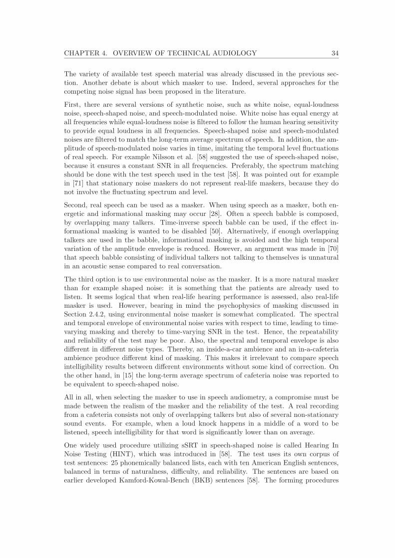
CHAPTER 4. OVERVIEW OF TECHNICAL AUDIOLOGY 34
The variety of available test speech material was already discussed in the previous sec-tion. Another debate is about which masker to use. Indeed, several approaches for thecompeting noise signal has been proposed in the literature.
First, there are several versions of synthetic noise, such as white noise, equal-loudnessnoise, speech-shaped noise, and speech-modulated noise. White noise has equal energy atall frequencies while equal-loudness noise is filtered to follow the human hearing sensitivityto provide equal loudness in all frequencies. Speech-shaped noise and speech-modulatednoises are filtered to match the long-term average spectrum of speech. In addition, the am-plitude of speech-modulated noise varies in time, imitating the temporal level fluctuationsof real speech. For example Nilsson et al. [58] suggested the use of speech-shaped noise,because it ensures a constant SNR in all frequencies. Preferably, the spectrum matchingshould be done with the test speech used in the test [58]. It was pointed out for examplein [71] that stationary noise maskers do not represent real-life maskers, because they donot involve the fluctuating spectrum and level.
Second, real speech can be used as a masker. When using speech as a masker, both en-ergetic and informational masking may occur [28]. Often a speech babble is composed,by overlapping many talkers. Time-inverse speech babble can be used, if the effect in-formational masking is wanted to be disabled [50]. Alternatively, if enough overlappingtalkers are used in the babble, informational masking is avoided and the high temporalvariation of the amplitude envelope is reduced. However, an argument was made in [70]that speech babble consisting of individual talkers not talking to themselves is unnaturalin an acoustic sense compared to real conversation.
The third option is to use environmental noise as the masker. It is a more natural maskerthan for example shaped noise: it is something that the patients are already used tolisten. It seems logical that when real-life hearing performance is assessed, also real-lifemasker is used. However, bearing in mind the psychophysics of masking discussed inSection 2.4.2, using environmental noise masker is somewhat complicated. The spectraland temporal envelope of environmental noise varies with respect to time, leading to time-varying masking and thereby to time-varying SNR in the test. Hence, the repeatabilityand reliability of the test may be poor. Also, the spectral and temporal envelope is alsodifferent in different noise types. Thereby, an inside-a-car ambience and an in-a-cafeteriaambience produce different kind of masking. This makes it irrelevant to compare speechintelligibility results between different environments without some kind of correction. Onthe other hand, in [15] the long-term average spectrum of cafeteria noise was reported tobe equivalent to speech-shaped noise.
All in all, when selecting the masker to use in speech audiometry, a compromise must bemade between the realism of the masker and the reliability of the test. A real recordingfrom a cafeteria consists not only of overlapping talkers but also of several non-stationarysound events. For example, when a loud knock happens in a middle of a word to belistened, speech intelligibility for that word is significantly lower than on average.
One widely used procedure utilizing sSRT in speech-shaped noise is called Hearing InNoise Testing (HINT), which was introduced in [58]. The test uses its own corpus oftest sentences: 25 phonemically balanced lists, each with ten American English sentences,balanced in terms of naturalness, difficulty, and reliability. The sentences are based onearlier developed Kamford-Kowal-Bench (BKB) sentences [58]. The forming procedures
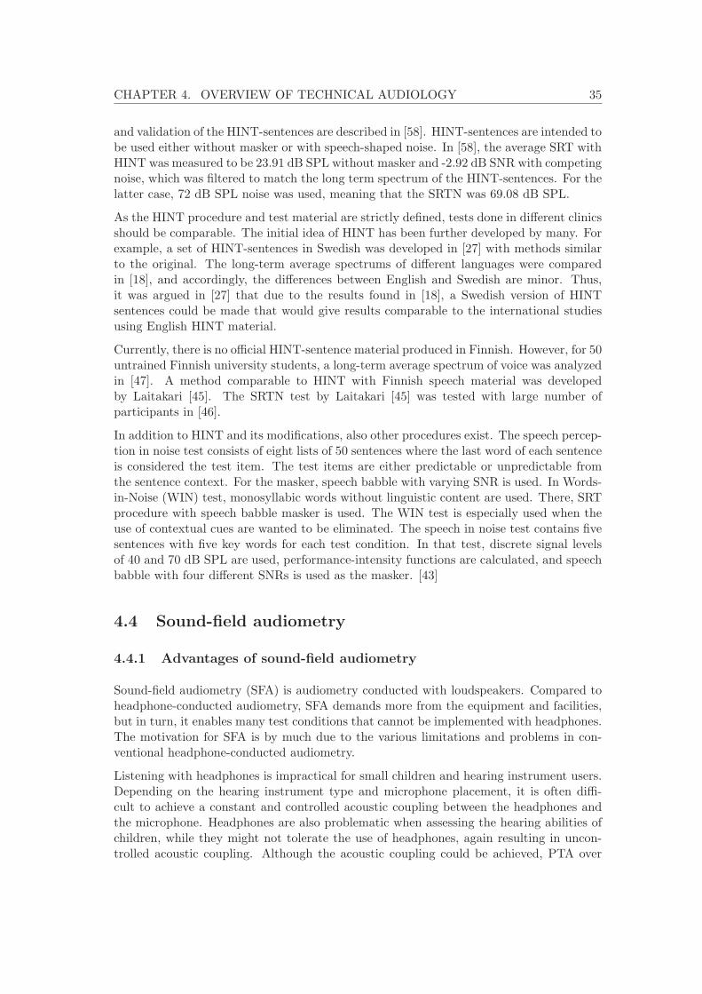
CHAPTER 4. OVERVIEW OF TECHNICAL AUDIOLOGY 35
and validation of the HINT-sentences are described in [58]. HINT-sentences are intended tobe used either without masker or with speech-shaped noise. In [58], the average SRT withHINT was measured to be 23.91 dB SPL without masker and -2.92 dB SNR with competingnoise, which was filtered to match the long term spectrum of the HINT-sentences. For thelatter case, 72 dB SPL noise was used, meaning that the SRTN was 69.08 dB SPL.
As the HINT procedure and test material are strictly defined, tests done in different clinicsshould be comparable. The initial idea of HINT has been further developed by many. Forexample, a set of HINT-sentences in Swedish was developed in [27] with methods similarto the original. The long-term average spectrums of different languages were comparedin [18], and accordingly, the differences between English and Swedish are minor. Thus,it was argued in [27] that due to the results found in [18], a Swedish version of HINTsentences could be made that would give results comparable to the international studiesusing English HINT material.
Currently, there is no official HINT-sentence material produced in Finnish. However, for 50untrained Finnish university students, a long-term average spectrum of voice was analyzedin [47]. A method comparable to HINT with Finnish speech material was developedby Laitakari [45]. The SRTN test by Laitakari [45] was tested with large number ofparticipants in [46].
In addition to HINT and its modifications, also other procedures exist. The speech percep-tion in noise test consists of eight lists of 50 sentences where the last word of each sentenceis considered the test item. The test items are either predictable or unpredictable fromthe sentence context. For the masker, speech babble with varying SNR is used. In Words-in-Noise (WIN) test, monosyllabic words without linguistic content are used. There, SRTprocedure with speech babble masker is used. The WIN test is especially used when theuse of contextual cues are wanted to be eliminated. The speech in noise test contains fivesentences with five key words for each test condition. In that test, discrete signal levelsof 40 and 70 dB SPL are used, performance-intensity functions are calculated, and speechbabble with four different SNRs is used as the masker. [43]
4.4 Sound-field audiometry
4.4.1 Advantages of sound-field audiometry
Sound-field audiometry (SFA) is audiometry conducted with loudspeakers. Compared toheadphone-conducted audiometry, SFA demands more from the equipment and facilities,but in turn, it enables many test conditions that cannot be implemented with headphones.The motivation for SFA is by much due to the various limitations and problems in con-ventional headphone-conducted audiometry.
Listening with headphones is impractical for small children and hearing instrument users.Depending on the hearing instrument type and microphone placement, it is often diffi-cult to achieve a constant and controlled acoustic coupling between the headphones andthe microphone. Headphones are also problematic when assessing the hearing abilities ofchildren, while they might not tolerate the use of headphones, again resulting in uncon-trolled acoustic coupling. Although the acoustic coupling could be achieved, PTA over
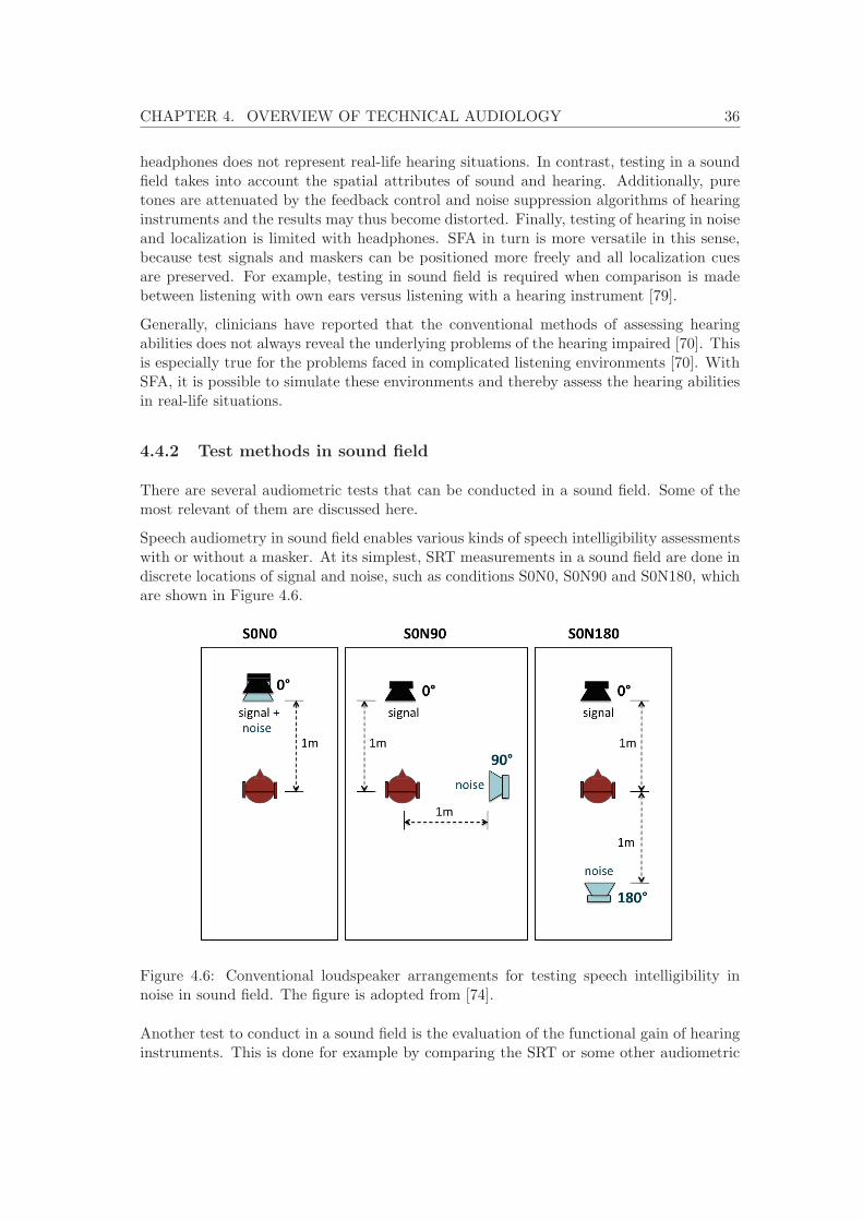
CHAPTER 4. OVERVIEW OF TECHNICAL AUDIOLOGY 36
headphones does not represent real-life hearing situations. In contrast, testing in a soundfield takes into account the spatial attributes of sound and hearing. Additionally, puretones are attenuated by the feedback control and noise suppression algorithms of hearinginstruments and the results may thus become distorted. Finally, testing of hearing in noiseand localization is limited with headphones. SFA in turn is more versatile in this sense,because test signals and maskers can be positioned more freely and all localization cuesare preserved. For example, testing in sound field is required when comparison is madebetween listening with own ears versus listening with a hearing instrument [79].
Generally, clinicians have reported that the conventional methods of assessing hearingabilities does not always reveal the underlying problems of the hearing impaired [70]. Thisis especially true for the problems faced in complicated listening environments [70]. WithSFA, it is possible to simulate these environments and thereby assess the hearing abilitiesin real-life situations.
4.4.2 Test methods in sound field
There are several audiometric tests that can be conducted in a sound field. Some of themost relevant of them are discussed here.
Speech audiometry in sound field enables various kinds of speech intelligibility assessmentswith or without a masker. At its simplest, SRT measurements in a sound field are done indiscrete locations of signal and noise, such as conditions S0N0, S0N90 and S0N180, whichare shown in Figure 4.6.
Figure 4.6: Conventional loudspeaker arrangements for testing speech intelligibility innoise in sound field. The figure is adopted from [74].
Another test to conduct in a sound field is the evaluation of the functional gain of hearinginstruments. This is done for example by comparing the SRT or some other audiometric
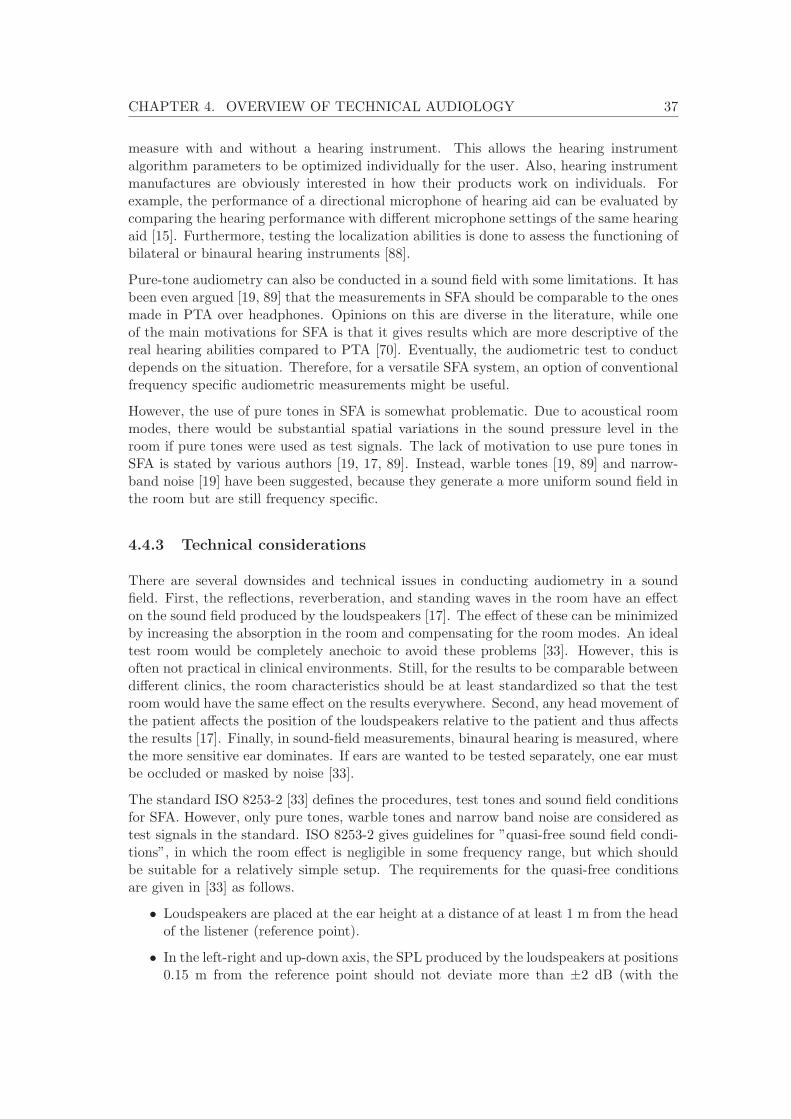
CHAPTER 4. OVERVIEW OF TECHNICAL AUDIOLOGY 37
measure with and without a hearing instrument. This allows the hearing instrumentalgorithm parameters to be optimized individually for the user. Also, hearing instrumentmanufactures are obviously interested in how their products work on individuals. Forexample, the performance of a directional microphone of hearing aid can be evaluated bycomparing the hearing performance with different microphone settings of the same hearingaid [15]. Furthermore, testing the localization abilities is done to assess the functioning ofbilateral or binaural hearing instruments [88].
Pure-tone audiometry can also be conducted in a sound field with some limitations. It hasbeen even argued [19, 89] that the measurements in SFA should be comparable to the onesmade in PTA over headphones. Opinions on this are diverse in the literature, while oneof the main motivations for SFA is that it gives results which are more descriptive of thereal hearing abilities compared to PTA [70]. Eventually, the audiometric test to conductdepends on the situation. Therefore, for a versatile SFA system, an option of conventionalfrequency specific audiometric measurements might be useful.
However, the use of pure tones in SFA is somewhat problematic. Due to acoustical roommodes, there would be substantial spatial variations in the sound pressure level in theroom if pure tones were used as test signals. The lack of motivation to use pure tones inSFA is stated by various authors [19, 17, 89]. Instead, warble tones [19, 89] and narrow-band noise [19] have been suggested, because they generate a more uniform sound field inthe room but are still frequency specific.
4.4.3 Technical considerations
There are several downsides and technical issues in conducting audiometry in a soundfield. First, the reflections, reverberation, and standing waves in the room have an effecton the sound field produced by the loudspeakers [17]. The effect of these can be minimizedby increasing the absorption in the room and compensating for the room modes. An idealtest room would be completely anechoic to avoid these problems [33]. However, this isoften not practical in clinical environments. Still, for the results to be comparable betweendifferent clinics, the room characteristics should be at least standardized so that the testroom would have the same effect on the results everywhere. Second, any head movement ofthe patient affects the position of the loudspeakers relative to the patient and thus affectsthe results [17]. Finally, in sound-field measurements, binaural hearing is measured, wherethe more sensitive ear dominates. If ears are wanted to be tested separately, one ear mustbe occluded or masked by noise [33].
The standard ISO 8253-2 [33] defines the procedures, test tones and sound field conditionsfor SFA. However, only pure tones, warble tones and narrow band noise are considered astest signals in the standard. ISO 8253-2 gives guidelines for ”quasi-free sound field condi-tions”, in which the room effect is negligible in some frequency range, but which shouldbe suitable for a relatively simple setup. The requirements for the quasi-free conditionsare given in [33] as follows.
• Loudspeakers are placed at the ear height at a distance of at least 1 m from the headof the listener (reference point).
• In the left-right and up-down axis, the SPL produced by the loudspeakers at positions0.15 m from the reference point should not deviate more than ±2 dB (with the
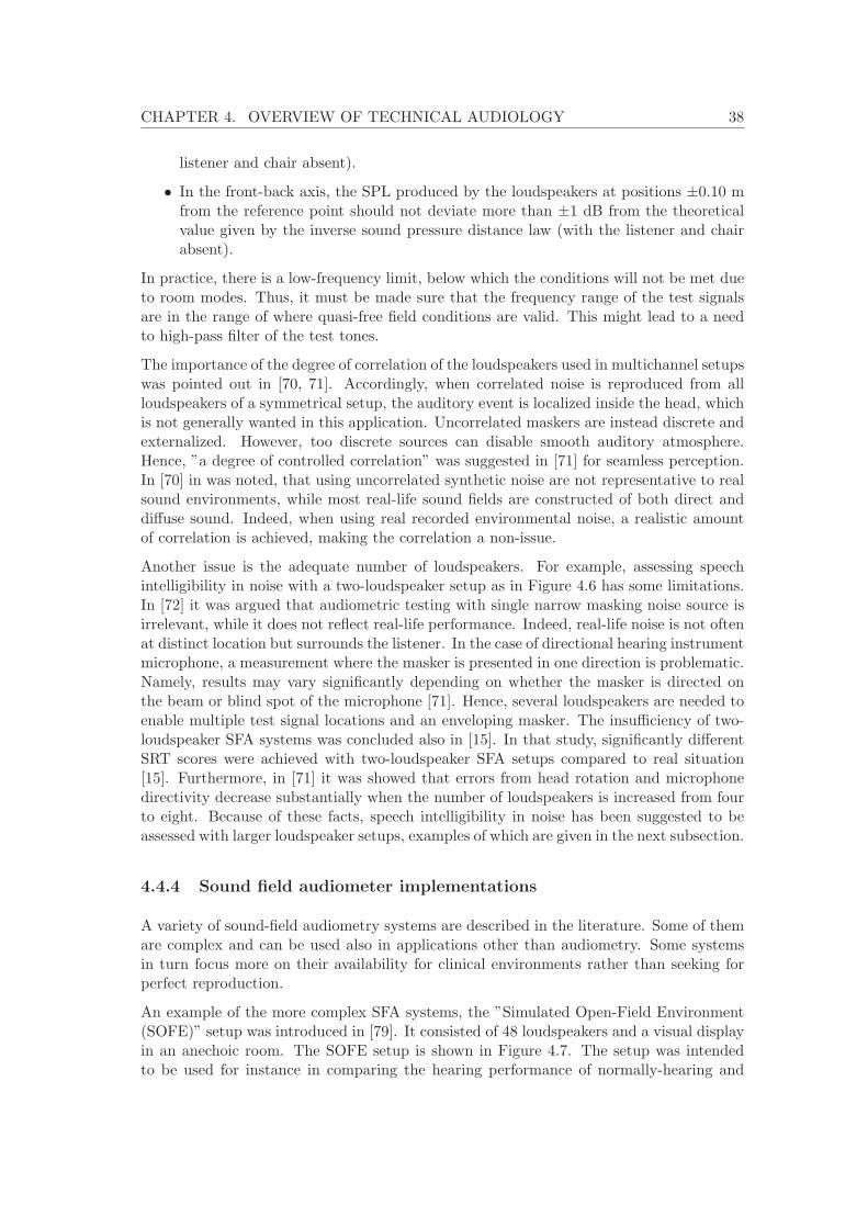
CHAPTER 4. OVERVIEW OF TECHNICAL AUDIOLOGY 38
listener and chair absent).
• In the front-back axis, the SPL produced by the loudspeakers at positions ±0.10 mfrom the reference point should not deviate more than ±1 dB from the theoreticalvalue given by the inverse sound pressure distance law (with the listener and chairabsent).
In practice, there is a low-frequency limit, below which the conditions will not be met dueto room modes. Thus, it must be made sure that the frequency range of the test signalsare in the range of where quasi-free field conditions are valid. This might lead to a needto high-pass filter of the test tones.
The importance of the degree of correlation of the loudspeakers used in multichannel setupswas pointed out in [70, 71]. Accordingly, when correlated noise is reproduced from allloudspeakers of a symmetrical setup, the auditory event is localized inside the head, whichis not generally wanted in this application. Uncorrelated maskers are instead discrete andexternalized. However, too discrete sources can disable smooth auditory atmosphere.Hence, ”a degree of controlled correlation” was suggested in [71] for seamless perception.In [70] in was noted, that using uncorrelated synthetic noise are not representative to realsound environments, while most real-life sound fields are constructed of both direct anddiffuse sound. Indeed, when using real recorded environmental noise, a realistic amountof correlation is achieved, making the correlation a non-issue.
Another issue is the adequate number of loudspeakers. For example, assessing speechintelligibility in noise with a two-loudspeaker setup as in Figure 4.6 has some limitations.In [72] it was argued that audiometric testing with single narrow masking noise source isirrelevant, while it does not reflect real-life performance. Indeed, real-life noise is not oftenat distinct location but surrounds the listener. In the case of directional hearing instrumentmicrophone, a measurement where the masker is presented in one direction is problematic.Namely, results may vary significantly depending on whether the masker is directed onthe beam or blind spot of the microphone [71]. Hence, several loudspeakers are needed toenable multiple test signal locations and an enveloping masker. The insufficiency of two-loudspeaker SFA systems was concluded also in [15]. In that study, significantly differentSRT scores were achieved with two-loudspeaker SFA setups compared to real situation[15]. Furthermore, in [71] it was showed that errors from head rotation and microphonedirectivity decrease substantially when the number of loudspeakers is increased from fourto eight. Because of these facts, speech intelligibility in noise has been suggested to beassessed with larger loudspeaker setups, examples of which are given in the next subsection.
4.4.4 Sound field audiometer implementations
A variety of sound-field audiometry systems are described in the literature. Some of themare complex and can be used also in applications other than audiometry. Some systemsin turn focus more on their availability for clinical environments rather than seeking forperfect reproduction.
An example of the more complex SFA systems, the ”Simulated Open-Field Environment(SOFE)” setup was introduced in [79]. It consisted of 48 loudspeakers and a visual displayin an anechoic room. The SOFE setup is shown in Figure 4.7. The setup was intendedto be used for instance in comparing the hearing performance of normally-hearing and
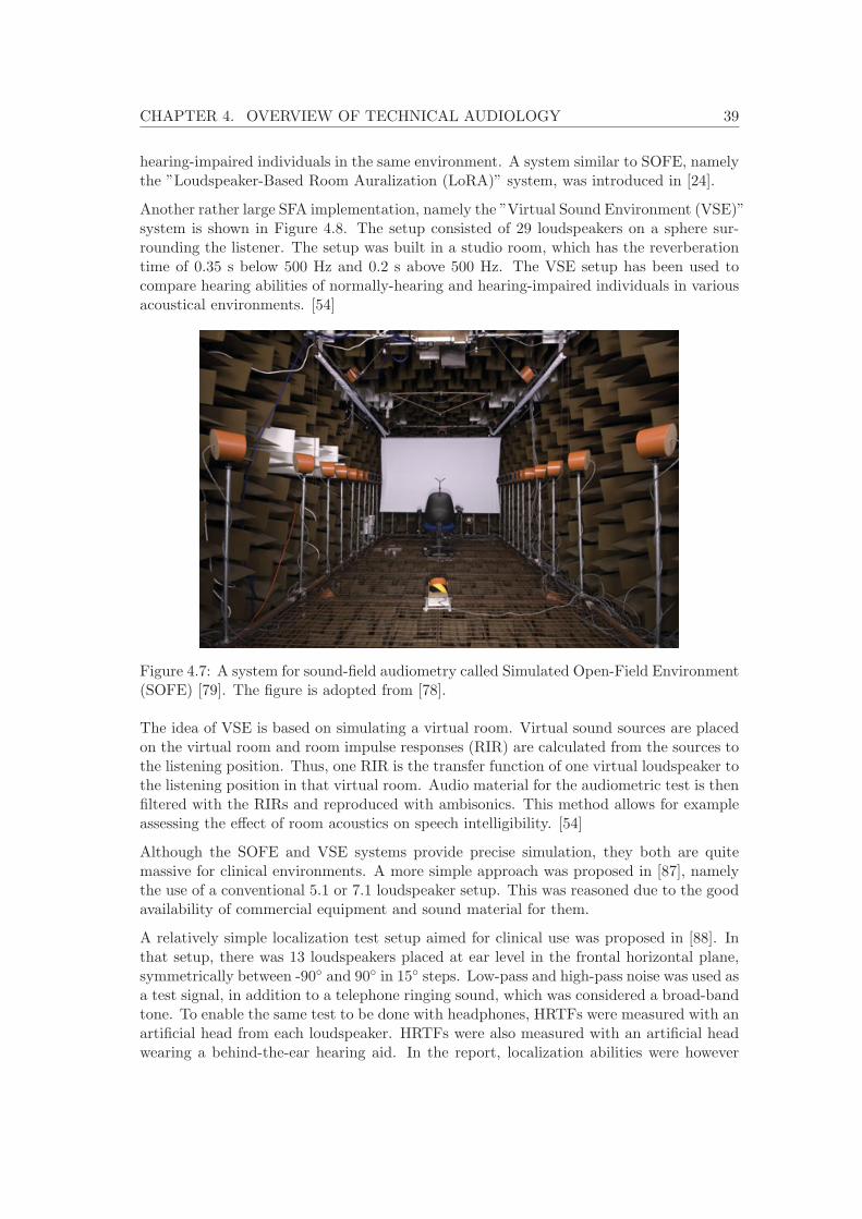
CHAPTER 4. OVERVIEW OF TECHNICAL AUDIOLOGY 39
hearing-impaired individuals in the same environment. A system similar to SOFE, namelythe ”Loudspeaker-Based Room Auralization (LoRA)” system, was introduced in [24].
Another rather large SFA implementation, namely the ”Virtual Sound Environment (VSE)”system is shown in Figure 4.8. The setup consisted of 29 loudspeakers on a sphere sur-rounding the listener. The setup was built in a studio room, which has the reverberationtime of 0.35 s below 500 Hz and 0.2 s above 500 Hz. The VSE setup has been used tocompare hearing abilities of normally-hearing and hearing-impaired individuals in variousacoustical environments. [54]
Figure 4.7: A system for sound-field audiometry called Simulated Open-Field Environment(SOFE) [79]. The figure is adopted from [78].
The idea of VSE is based on simulating a virtual room. Virtual sound sources are placedon the virtual room and room impulse responses (RIR) are calculated from the sources tothe listening position. Thus, one RIR is the transfer function of one virtual loudspeaker tothe listening position in that virtual room. Audio material for the audiometric test is thenfiltered with the RIRs and reproduced with ambisonics. This method allows for exampleassessing the effect of room acoustics on speech intelligibility. [54]
Although the SOFE and VSE systems provide precise simulation, they both are quitemassive for clinical environments. A more simple approach was proposed in [87], namelythe use of a conventional 5.1 or 7.1 loudspeaker setup. This was reasoned due to the goodavailability of commercial equipment and sound material for them.
A relatively simple localization test setup aimed for clinical use was proposed in [88]. Inthat setup, there was 13 loudspeakers placed at ear level in the frontal horizontal plane,symmetrically between -90◦ and 90◦ in 15◦ steps. Low-pass and high-pass noise was used asa test signal, in addition to a telephone ringing sound, which was considered a broad-bandtone. To enable the same test to be done with headphones, HRTFs were measured with anartificial head from each loudspeaker. HRTFs were also measured with an artificial headwearing a behind-the-ear hearing aid. In the report, localization abilities were however
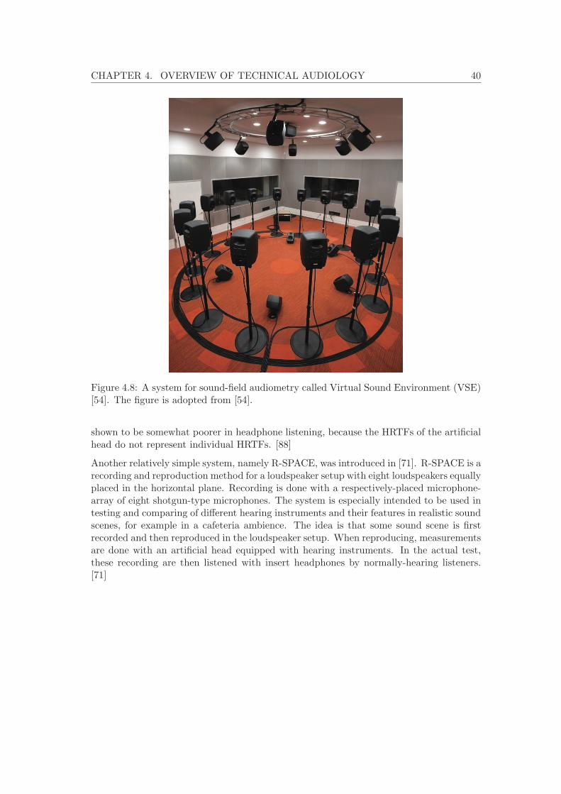
CHAPTER 4. OVERVIEW OF TECHNICAL AUDIOLOGY 40
Figure 4.8: A system for sound-field audiometry called Virtual Sound Environment (VSE)[54]. The figure is adopted from [54].
shown to be somewhat poorer in headphone listening, because the HRTFs of the artificialhead do not represent individual HRTFs. [88]
Another relatively simple system, namely R-SPACE, was introduced in [71]. R-SPACE is arecording and reproduction method for a loudspeaker setup with eight loudspeakers equallyplaced in the horizontal plane. Recording is done with a respectively-placed microphone-array of eight shotgun-type microphones. The system is especially intended to be used intesting and comparing of different hearing instruments and their features in realistic soundscenes, for example in a cafeteria ambience. The idea is that some sound scene is firstrecorded and then reproduced in the loudspeaker setup. When reproducing, measurementsare done with an artificial head equipped with hearing instruments. In the actual test,these recording are then listened with insert headphones by normally-hearing listeners.[71]
Chapter 5
DirAC-based sound-fieldaudiometry
Section 3.2 introduced a spatial audio technique called Directional Audio Coding (DirAC)and Section 4.4 explored the concept of sound-field audiometry (SFA). In the followingchapter, a concept of sound-field audiometry system utilizing DirAC is described andmotivated. Also prototyping and brief technical validation of the concept is reported.
5.1 The overall concept
The fundamental idea in DirAC-based sound-field audiometry is to enable hearing per-formance assessments in reproduced sound scenes with reasonable technical requirements.Using the term ”reproduced sound scenes” emphasizes the fact that nothing is simu-lated, but existing sound environments are recorded and reproduced. Thereby, realismis achieved naturally. To be precise, however, sound scene reproduction is mixed withaugmentation of external sound events.
The overall concept of DirAC-based sound-field audiometry is illustrated in Figure 5.1.The black box in the figure represents the SFA system itself, the contents of which aredescribed in the next section. To reproduce any given sound scene, the system needstwo inputs from the real environment to be reproduced. First, the background noise isrecorded in A-format. Second, the acoustical properties of the environment are captured inan A-format spatial impulse response. The third input is an anechoic speech corpus. Thetalker of this corpus is then augmented to the sound scene using the measured acousticalproperties of that environment. The system outputs the loudspeaker signals for arbitrarynumber of loudspeakers in arbitrary locations.
When the sound scene with the augmented talker is reproduced in the SFA setup, thelistener is not only enveloped by the sound scene of the real environment, but also hearsthe talker in the speech corpus as if he/she was also there in the real environment. Thereby,speech intelligibility assessments, for example a SRT test in noise, can be made in realisticenvironments, using the background sound scene as the masker and the augmented talkeras the test speech. Now that the anechoic speech corpus and environment recordings areseparated, different speech materials can be flexibly combined with different background
41

CHAPTER 5. DIRAC-BASED SOUND-FIELD AUDIOMETRY 42
scenes. This is advantageous, since the speech corpus itself does not have to be recordedin the real environment. That is, the system is compatible with any existing speechcorpus. Also, sound scenes can be recorded anywhere with relatively simple methods.Consequently, speech intelligibility assessments can be virtually done, for example, in ahighly-reverberant railway station lobby, or some specific cafeteria, depending on whatkind of scenarios are of interest. Although the discussion in this thesis is limited to speechintelligibility assessments in noise, the presented concept is not necessarily limited to them.
The presented concept is motivated mainly by the limitations of traditional audiometricmethods in measuring real-life hearing performance. With this concept, the patient, al-though physically in the clinic, can be virtually transported to the sound scene of a realenvironment of choice. Another advantage in the concept is that loudspeaker signals arenaturally uncorrelated. On the contrary, if an omnidirectional recording of the backgroundnoise was reproduced with several loudspeakers, the loudspeaker channels would correlate.
Real environment
SFA setup at clinic
Background
noise (n)
Room
acoustics spatial impulse
response H(f )
H(f )
n Anechoic
speech corpus
Figure 5.1: The overall concept of DirAC-based sound-field audiometry.
5.2 Description of the SFA system
5.2.1 Reproducing a sound scene
The black box in Figure 5.1 represents the SFA system itself, consisting of the chain ofoperations from the original recorded audio material to the final loudspeaker signals forthe test setup. A high-level block diagram of this black box is presented in Figure 5.2.The signal flow consists of two separate audio streams, namely the masker stream (from
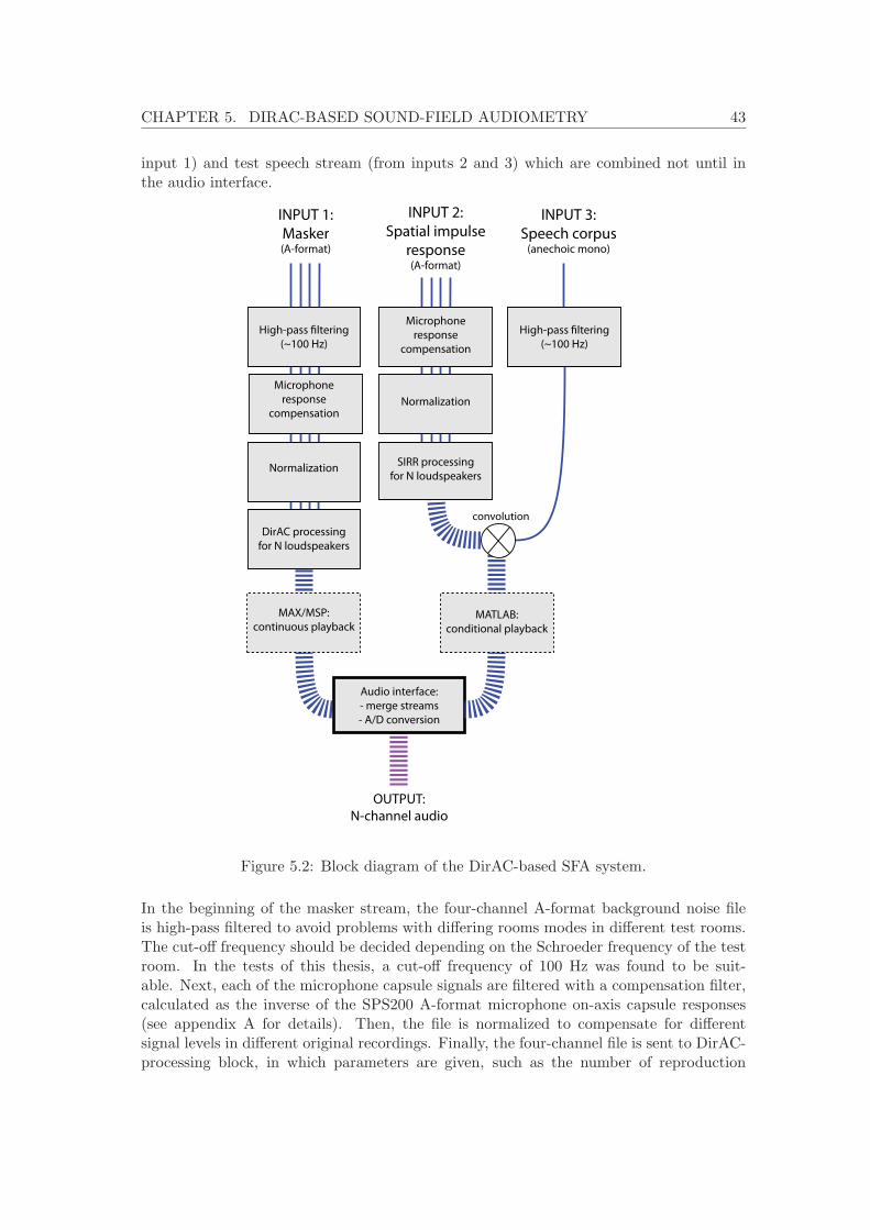
CHAPTER 5. DIRAC-BASED SOUND-FIELD AUDIOMETRY 43
input 1) and test speech stream (from inputs 2 and 3) which are combined not until inthe audio interface.
INPUT 1:
Masker (A-format)
Audio interface:
- merge streams
- A/D conversion
MAX/MSP:
continuous playback
Microphone
response
compensation
Normalization
SIRR processing
for N loudspeakers
INPUT 2:
Spatial impulse
response (A-format)
INPUT 3:
Speech corpus(anechoic mono)
High-pass filtering
(~100 Hz)
MATLAB:
conditional playback
High-pass filtering
(~100 Hz)
Microphone
response
compensation
Normalization
DirAC processing
for N loudspeakers
convolution
OUTPUT:
N-channel audio
Figure 5.2: Block diagram of the DirAC-based SFA system.
In the beginning of the masker stream, the four-channel A-format background noise fileis high-pass filtered to avoid problems with differing rooms modes in different test rooms.The cut-off frequency should be decided depending on the Schroeder frequency of the testroom. In the tests of this thesis, a cut-off frequency of 100 Hz was found to be suit-able. Next, each of the microphone capsule signals are filtered with a compensation filter,calculated as the inverse of the SPS200 A-format microphone on-axis capsule responses(see appendix A for details). Then, the file is normalized to compensate for differentsignal levels in different original recordings. Finally, the four-channel file is sent to DirAC-processing block, in which parameters are given, such as the number of reproduction
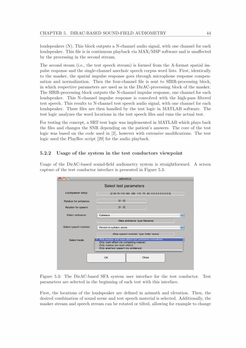
CHAPTER 5. DIRAC-BASED SOUND-FIELD AUDIOMETRY 44
loudspeakers (N). This block outputs a N-channel audio signal, with one channel for eachloudspeaker. This file is in continuous playback via MAX/MSP software and is unaffectedby the processing in the second stream.
The second steam (i.e., the test speech stream) is formed from the A-format spatial im-pulse response and the single-channel anechoic speech corpus word lists. First, identicallyto the masker, the spatial impulse response goes through microphone response compen-sation and normalization. Then the four-channel file is sent to SIRR-processing block,in which respective parameters are used as in the DirAC-processing block of the masker.The SIRR-processing block outputs the N-channel impulse response, one channel for eachloudspeaker. This N-channel impulse response is convolved with the high-pass filteredtest speech. This results to N-channel test speech audio signal, with one channel for eachloudspeaker. These files are then handled by the test logic in MATLAB software. Thetest logic analyzes the word locations in the test speech files and runs the actual test.
For testing the concept, a SRT-test logic was implemented in MATLAB which plays backthe files and changes the SNR depending on the patient’s answers. The core of the testlogic was based on the code used in [2], however with extensive modifications. The testlogic used the PlayRec script [29] for the audio playback.
5.2.2 Usage of the system in the test conductors viewpoint
Usage of the DirAC-based sound-field audiometry system is straightforward. A screencapture of the test conductor interface is presented in Figure 5.3.
Figure 5.3: The DirAC-based SFA system user interface for the test conductor. Testparameters are selected in the beginning of each test with this interface.
First, the locations of the loudspeaker are defined in azimuth and elevation. Then, thedesired combination of sound scene and test speech material is selected. Additionally, themasker stream and speech stream can be rotated or tilted, allowing for example to change
CHAPTER 5. DIRAC-BASED SOUND-FIELD AUDIOMETRY 45
the talker location. It is also possible to conduct the test without a masker or without aroom effect. In the latter case, anechoic speech is used. After setting the test parameters,an interface for the listener opens up, including a bare text field for the answers and thetest can begin. Another figure opens up for the test conductor where the adaptive trackcan be monitored.
As all the three inputs are separated, combinations can be done flexibly. That is, it ispossible to combine a masker from one real environment to room acoustics from anotherenvironment. This was not however implemented in the interface shown in the figure,because the system was wanted to keep as simple and usable as possible. Anyhow, oneof the advantages of the software is its modularity. Namely, if new inputs are wanted tobe used, they can be flexibly added to the system by just typing a folder name where theaudio files are located. Thus, the end user is not restricted to use the supported soundscenes, but is able to import new test speech material or even own A-format recordings.
5.3 Prototyping
5.3.1 On the test environments
For prototyping of the concept, three test environments were built. First of all, a referenceenvironment was built to represent a real-life situation. Then, two SFA prototype setupswere built. First of the prototypes represents clinical setup, a setup compact enoughthat could be implemented in an audiometric clinic. The second prototype represents anideal setup in anechoic conditions, a setup free from the additional room effect of the testroom. The sound scene in the reference environment was captured and then reproducedin the two prototype setups following the methods introduced previously in this chapter.The environments were arranged so that the same SRT test could be done in all threeenvironments. In the next three subsections, the test environments are described.
5.3.2 Reference environment
The reference environment was designed to represent a realistic environment with back-ground noise and reverberation, such as a crowded cafeteria. Real environments usuallyhave a non-stationary background noise, but using such would induce reliability issuesto the actual audiometric test. Thus, a conscious compromise between realism and testreliability was made: the background noise was restricted to be rather stationary.
The reference environment was built in a relatively big room equipped with eight activeloudspeakers (Genelec 1030A) placed fairly uniformly around the room. Each of theseloudspeakers were tilted differently in elevation and directed towards wall, bookshelf, orother reflective and diffusive surface. This was done to avoid direct sound from these loud-speakers to the listener position and to make the sound field as diffuse and enveloping aspossible. Anechoic 18-talker speech babble was played back from these eight loudspeakersas the background noise. The babble was mixed from anechoic recordings of nine differentmale talkers. The recorded material consisted of complete sentences in Finnish. Due tothat many overlapping talkers, the informational content in the sentences could not be
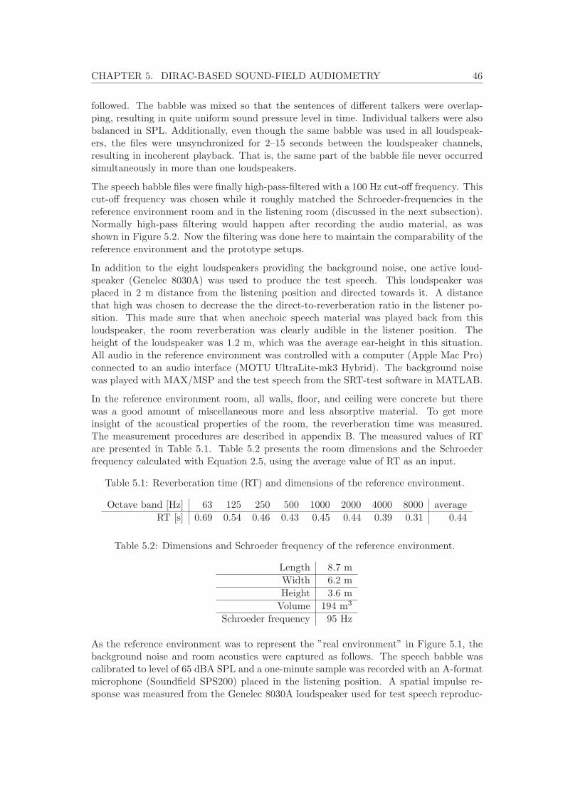
CHAPTER 5. DIRAC-BASED SOUND-FIELD AUDIOMETRY 46
followed. The babble was mixed so that the sentences of different talkers were overlap-ping, resulting in quite uniform sound pressure level in time. Individual talkers were alsobalanced in SPL. Additionally, even though the same babble was used in all loudspeak-ers, the files were unsynchronized for 2–15 seconds between the loudspeaker channels,resulting in incoherent playback. That is, the same part of the babble file never occurredsimultaneously in more than one loudspeakers.
The speech babble files were finally high-pass-filtered with a 100 Hz cut-off frequency. Thiscut-off frequency was chosen while it roughly matched the Schroeder-frequencies in thereference environment room and in the listening room (discussed in the next subsection).Normally high-pass filtering would happen after recording the audio material, as wasshown in Figure 5.2. Now the filtering was done here to maintain the comparability of thereference environment and the prototype setups.
In addition to the eight loudspeakers providing the background noise, one active loud-speaker (Genelec 8030A) was used to produce the test speech. This loudspeaker wasplaced in 2 m distance from the listening position and directed towards it. A distancethat high was chosen to decrease the the direct-to-reverberation ratio in the listener po-sition. This made sure that when anechoic speech material was played back from thisloudspeaker, the room reverberation was clearly audible in the listener position. Theheight of the loudspeaker was 1.2 m, which was the average ear-height in this situation.All audio in the reference environment was controlled with a computer (Apple Mac Pro)connected to an audio interface (MOTU UltraLite-mk3 Hybrid). The background noisewas played with MAX/MSP and the test speech from the SRT-test software in MATLAB.
In the reference environment room, all walls, floor, and ceiling were concrete but therewas a good amount of miscellaneous more and less absorptive material. To get moreinsight of the acoustical properties of the room, the reverberation time was measured.The measurement procedures are described in appendix B. The measured values of RTare presented in Table 5.1. Table 5.2 presents the room dimensions and the Schroederfrequency calculated with Equation 2.5, using the average value of RT as an input.
Table 5.1: Reverberation time (RT) and dimensions of the reference environment.
Octave band [Hz] 63 125 250 500 1000 2000 4000 8000 average
RT [s] 0.69 0.54 0.46 0.43 0.45 0.44 0.39 0.31 0.44
Table 5.2: Dimensions and Schroeder frequency of the reference environment.
Length 8.7 m
Width 6.2 m
Height 3.6 m
Volume 194 m3
Schroeder frequency 95 Hz
As the reference environment was to represent the ”real environment” in Figure 5.1, thebackground noise and room acoustics were captured as follows. The speech babble wascalibrated to level of 65 dBA SPL and a one-minute sample was recorded with an A-formatmicrophone (Soundfield SPS200) placed in the listening position. A spatial impulse re-sponse was measured from the Genelec 8030A loudspeaker used for test speech reproduc-

CHAPTER 5. DIRAC-BASED SOUND-FIELD AUDIOMETRY 47
tion to the Soundfield SPS200 microphone in the listening position. The measurementwas done using a logarithmic sine sweep and post-processing procedures similar to whichwere explained in [52], a report describing similar measurements done in a concert hall.All measurements were done in MATLAB environment with a computer (Apple Macbook)connected to an audio interface (MOTU Traveler mk3).
5.3.3 The listening room prototype setup
The first prototype for the DirAC-based SFA system was built in a listening room thatmeets the ITU-R BS.1116 [35] listening room recommendations. This setup was to rep-resent a clinical setup in terms of the room size and acoustics. The room was equippedwith nine active loudspeakers (Genelec 8260A) in floor stands and four active loudspeakers(Genelec 8240A) attached to the ceiling. The number of loudspeakers used and their loca-tion was varied during the validation process. All audio was played back with a computer(Apple Macbook) connected to a digital mixer (Yamaha 02R96) via an audio interface(RME Fireface 800).
Reverberation time in the listening room was measured using measurement proceduresdescribed in appendix B. The measured values of RT are presented in Table 5.3. Table5.4 presents the room dimensions and the Schroeder frequency calculated with Equation2.5, using the average value of RT as an input.
Table 5.3: Reverberation time (RT) and dimensions of the listening room prototype setup.
Octave band [Hz] 63 125 250 500 1000 2000 4000 8000 average
RT [s] 0.42 0.38 0.23 0.25 0.26 0.27 0.26 0.23 0.26
Table 5.4: Dimensions and Schroeder frequency of the listening room prototype setup.
Length 6.3 m
Width 5.6 m
Height 2.7 m
Volume 95 m3
Schroeder frequency 105 Hz
5.3.4 The anechoic prototype setup
The second prototype for the DirAC-based sound-field audiometry system was built in ananechoic chamber. This setup was to represent the ideal setup in terms of room acoustics.The chamber was equipped with active loudspeakers (Genelec 8030A) in a transformable3D-setup. All audio was played back with a computer (Apple Mac Pro) connected to anaudio interface (MOTU 2408 mk3).
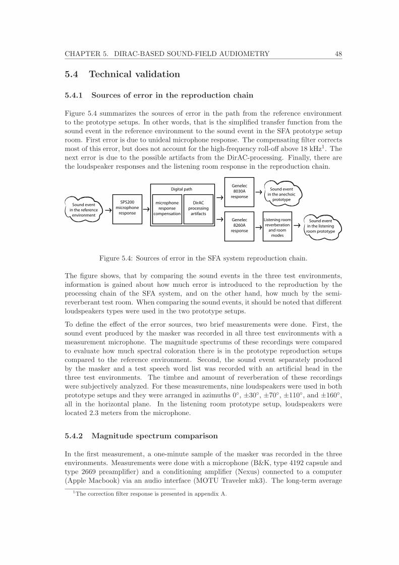
CHAPTER 5. DIRAC-BASED SOUND-FIELD AUDIOMETRY 48
5.4 Technical validation
5.4.1 Sources of error in the reproduction chain
Figure 5.4 summarizes the sources of error in the path from the reference environmentto the prototype setups. In other words, that is the simplified transfer function from thesound event in the reference environment to the sound event in the SFA prototype setuproom. First error is due to unideal microphone response. The compensating filter correctsmost of this error, but does not account for the high-frequency roll-off above 18 kHz1. Thenext error is due to the possible artifacts from the DirAC-processing. Finally, there arethe loudspeaker responses and the listening room response in the reproduction chain.
SPS200
microphone
response
microphone
response
compensation
DirAC
processing
artifacts
Genelec
8030A
response
Genelec
8260A
response
Listening room
reverberation
and room
modes
Sound event
in the reference
environment
Sound event
in the anechoic
prototype
Sound event
in the listening
room prototype
Digital path
Figure 5.4: Sources of error in the SFA system reproduction chain.
The figure shows, that by comparing the sound events in the three test environments,information is gained about how much error is introduced to the reproduction by theprocessing chain of the SFA system, and on the other hand, how much by the semi-reverberant test room. When comparing the sound events, it should be noted that differentloudspeakers types were used in the two prototype setups.
To define the effect of the error sources, two brief measurements were done. First, thesound event produced by the masker was recorded in all three test environments with ameasurement microphone. The magnitude spectrums of these recordings were comparedto evaluate how much spectral coloration there is in the prototype reproduction setupscompared to the reference environment. Second, the sound event separately producedby the masker and a test speech word list was recorded with an artificial head in thethree test environments. The timbre and amount of reverberation of these recordingswere subjectively analyzed. For these measurements, nine loudspeakers were used in bothprototype setups and they were arranged in azimuths 0◦, ±30◦, ±70◦, ±110◦, and ±160◦,all in the horizontal plane. In the listening room prototype setup, loudspeakers werelocated 2.3 meters from the microphone.
5.4.2 Magnitude spectrum comparison
In the first measurement, a one-minute sample of the masker was recorded in the threeenvironments. Measurements were done with a microphone (B&K, type 4192 capsule andtype 2669 preamplifier) and a conditioning amplifier (Nexus) connected to a computer(Apple Macbook) via an audio interface (MOTU Traveler mk3). The long-term average
1The correction filter response is presented in appendix A.
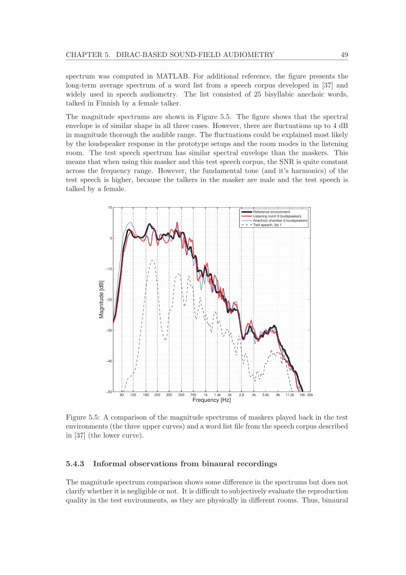
CHAPTER 5. DIRAC-BASED SOUND-FIELD AUDIOMETRY 49
spectrum was computed in MATLAB. For additional reference, the figure presents thelong-term average spectrum of a word list from a speech corpus developed in [37] andwidely used in speech audiometry. The list consisted of 25 bisyllabic anechoic words,talked in Finnish by a female talker.
The magnitude spectrums are shown in Figure 5.5. The figure shows that the spectralenvelope is of similar shape in all three cases. However, there are fluctuations up to 4 dBin magnitude thorough the audible range. The fluctuations could be explained most likelyby the loudspeaker response in the prototype setups and the room modes in the listeningroom. The test speech spectrum has similar spectral envelope than the maskers. Thismeans that when using this masker and this test speech corpus, the SNR is quite constantacross the frequency range. However, the fundamental tone (and it’s harmonics) of thetest speech is higher, because the talkers in the masker are male and the test speech istalked by a female.
90 125 180 250 350 500 700 1k 1.4k 2k 2.8 4k 5.6k 8k 11.2k 16k 20k−50
−40
−30
−20
−10
0
10
Frequency [Hz]
Mag
nitu
de [d
B]
Reference environmentListening room 9 loudspeakersAnechoic chamber 9 loudspeakersTest speech, list 1
Figure 5.5: A comparison of the magnitude spectrums of maskers played back in the testenvironments (the three upper curves) and a word list file from the speech corpus describedin [37] (the lower curve).
5.4.3 Informal observations from binaural recordings
The magnitude spectrum comparison shows some difference in the spectrums but does notclarify whether it is negligible or not. It is difficult to subjectively evaluate the reproductionquality in the test environments, as they are physically in different rooms. Thus, binaural
CHAPTER 5. DIRAC-BASED SOUND-FIELD AUDIOMETRY 50
recordings of the masker and test speech were made in all the three test environments.The same masker and speech corpus word list that was used in the magnitude spectrumcomparison were played back and recorded in the three environments. For the test speechthis means that in the reference environment the original anechoic word list was used andin the prototype setups the SIRR-processed list was used – just as it is done when a SRTtest in the system is conducted. These measurements were done with an artificial head(Cortex Manikin MK1) connected to a computer (Apple Macbook) via an audio interface(MOTU Traveler mk3).
The binaural recordings were carefully listened with headphones (Sennheiser HD800) bythe author. The recordings from the prototype setups were compared to the ones fromthe reference environment. Ideally, there should be no audible difference between these.Observations were made as follows, concerning spectral coloration and possible excessreverberation in the reproduction.
First of all, coloration was slightly audible in the maskers in both prototype setups. On theother hand, in the maskers there were no significant coloration audible and especially thespeech recordings from the anechoic prototype and the reference environment was reallyhard to tell apart.
Secondly, there was some excess room effect audible in the speech recording from thelistening room prototype. This is obvious, while there is an extra room response involved,namely the physical one of the listening room. However, this was not audible in thecontinuous masker recordings.
Finally, there was no excessive room effect in the recordings from the anechoic prototype.This was a clear improvement compared to what was achieved with B-format DirAC-processing. Namely, the same binaural measurements were conducted earlier by the authorusing DirAC-processing with B-format input signals. In those recordings, a clearly audibleincrease in the room effect was noticed, initially motivating the use of A-format DirAC-processing in this application. This finding gives further evidence for the note in [61]:compared to B-format processing, A-format DirAC-processing is more precise with thediffuseness estimate in high frequencies. Indeed, now with A-format DirAC-processing,there was no audible increase in room effect, while the diffuseness was not overestimated.
5.4.4 Conclusions
Based on the magnitude spectrum comparison, there were some differences in the spectralcontent of the maskers in the SFA prototype setups compared to reference environment.Also, this difference could be subjectively noticed by listening recordings of the respectivemaskers. In the case of test speech, the subjective difference was negligible. These find-ings emphasize the complexity of the sound scene reproduction system: there are manycascaded factors affecting to the final sound event. The technical validation suggestedthat the system could be valid, but did not prove it. This gives motivation for furthervalidation with listening tests, which are reported in the next chapter.

Chapter 6
Subjective listening tests
The psychoacoustic listening tests reported in this chapter were made to further evalu-ate whether the concept of DirAC-based sound-field audiometry is valid. The concept isconsidered valid, if equal scores of some audiometric measure can be recorded in a realenvironment and in a DirAC-based SFA setup in which the first mentioned is reproduced.If this criterion is met, hearing diagnosis made in a DirAC-based SFA setup can be con-sidered to represent real-life hearing performance in terms of that particular audiometricmeasure. Furthermore, the listening tests are aimed to suggest the adequate number ofloudspeakers and the requirements for the test room acoustics, with which the validitycriterion is met.
6.1 Test method in general
To test the equal speech intelligibility between the reference of real environment andits DirAC-reproduced equivalent, a set of listening test was conducted, where the testsubject went though a SRT-test in a real environment and corresponding reproductionenvironments. The reference environment described in Section 5.3.2 was used as the realenvironment and the prototype setups described in Sections 5.3.3 and 5.3.4 were used as thereproduction environments. Test procedures were the same as if speech audiometry withSRT-procedure was conducted. Thus, the validity criterion is met if the test environmenthas no effect on the SRT. This is proved if there is no statistically significant differencebetween the SRTs recorded in the different environments and the data used in the analysishas confidence intervals not larger than what would be accepted as an error in clinicalSRT-measurement.
Total of three separate listening tests were made and they are reported in Sections 6.2–6.4.In all three experiments, a SRT test procedure was used with the same speech material.Test A was somewhat a preliminary experiment for piloting the concept. Based on theinformation gained from that experiment, the test arrangement was refined for tests Band C. In test B, normal hearing test subjects were used and in test C the procedurewas repeated with hearing-impaired test subjects, who all had either hearing aid, cochlearimplant, or both in use. In all three tests, the general test method was similar to allowcomparison. Figure 6.1 summarizes the listening test setups.
51

CHAPTER 6. SUBJECTIVE LISTENING TESTS 52
2 m
tests A & C
test B
Listening room prototype setup Anechoic prototype setup
Reference environment
d
d = 2.3 m (test A), 1.0 m (tests B & C)
tests A & C
test B
tests A & C
test B
Speech babble loudspeakers
Anechoic test speech loudspeaker
Reproduction loudspeakers
Figure 6.1: The listening test setups. The arrows indicate the test subject orientation.
6.2 Test A
6.2.1 Introduction
For each test subject, SRT was measured in the following scenarios.
1. MON* - Mono reproduction in the listening room prototype with one loudspeaker
2. LR5* - DirAC-reproduction in the listening room prototype with five loudspeakers
3. LR9* - DirAC-reproduction in the listening room prototype with nine loudspeakers
4. LR13* - DirAC-reproduction in the listening room prototype with 13 loudspeakers
5. LRA* - Anechoic test speech and DirAC-reproduced masker in the listening roomprototype with 13 loudspeakers
6. REF - The reference environment
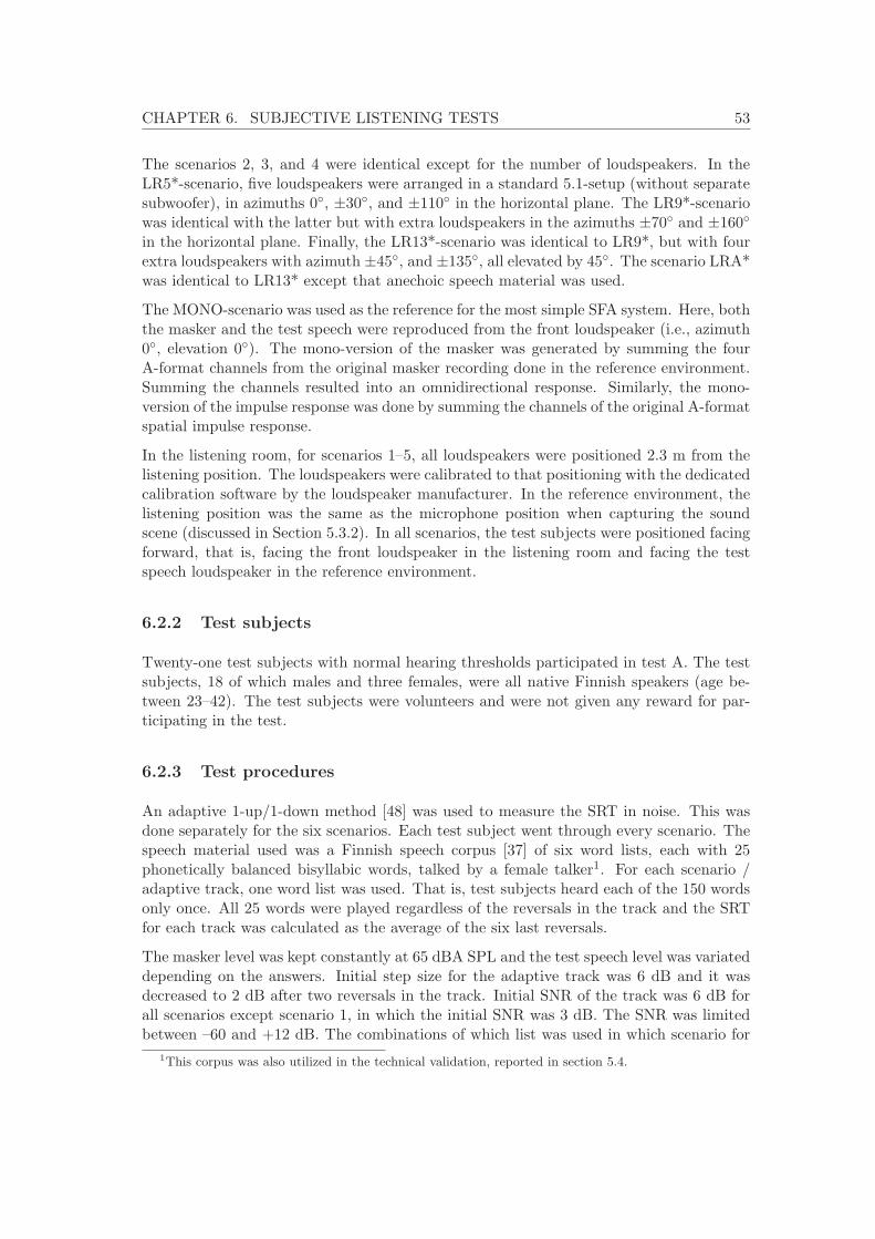
CHAPTER 6. SUBJECTIVE LISTENING TESTS 53
The scenarios 2, 3, and 4 were identical except for the number of loudspeakers. In theLR5*-scenario, five loudspeakers were arranged in a standard 5.1-setup (without separatesubwoofer), in azimuths 0◦, ±30◦, and ±110◦ in the horizontal plane. The LR9*-scenariowas identical with the latter but with extra loudspeakers in the azimuths ±70◦ and ±160◦
in the horizontal plane. Finally, the LR13*-scenario was identical to LR9*, but with fourextra loudspeakers with azimuth ±45◦, and ±135◦, all elevated by 45◦. The scenario LRA*was identical to LR13* except that anechoic speech material was used.
The MONO-scenario was used as the reference for the most simple SFA system. Here, boththe masker and the test speech were reproduced from the front loudspeaker (i.e., azimuth0◦, elevation 0◦). The mono-version of the masker was generated by summing the fourA-format channels from the original masker recording done in the reference environment.Summing the channels resulted into an omnidirectional response. Similarly, the mono-version of the impulse response was done by summing the channels of the original A-formatspatial impulse response.
In the listening room, for scenarios 1–5, all loudspeakers were positioned 2.3 m from thelistening position. The loudspeakers were calibrated to that positioning with the dedicatedcalibration software by the loudspeaker manufacturer. In the reference environment, thelistening position was the same as the microphone position when capturing the soundscene (discussed in Section 5.3.2). In all scenarios, the test subjects were positioned facingforward, that is, facing the front loudspeaker in the listening room and facing the testspeech loudspeaker in the reference environment.
6.2.2 Test subjects
Twenty-one test subjects with normal hearing thresholds participated in test A. The testsubjects, 18 of which males and three females, were all native Finnish speakers (age be-tween 23–42). The test subjects were volunteers and were not given any reward for par-ticipating in the test.
6.2.3 Test procedures
An adaptive 1-up/1-down method [48] was used to measure the SRT in noise. This wasdone separately for the six scenarios. Each test subject went through every scenario. Thespeech material used was a Finnish speech corpus [37] of six word lists, each with 25phonetically balanced bisyllabic words, talked by a female talker1. For each scenario /adaptive track, one word list was used. That is, test subjects heard each of the 150 wordsonly once. All 25 words were played regardless of the reversals in the track and the SRTfor each track was calculated as the average of the six last reversals.
The masker level was kept constantly at 65 dBA SPL and the test speech level was variateddepending on the answers. Initial step size for the adaptive track was 6 dB and it wasdecreased to 2 dB after two reversals in the track. Initial SNR of the track was 6 dB forall scenarios except scenario 1, in which the initial SNR was 3 dB. The SNR was limitedbetween –60 and +12 dB. The combinations of which list was used in which scenario for
1This corpus was also utilized in the technical validation, reported in section 5.4.
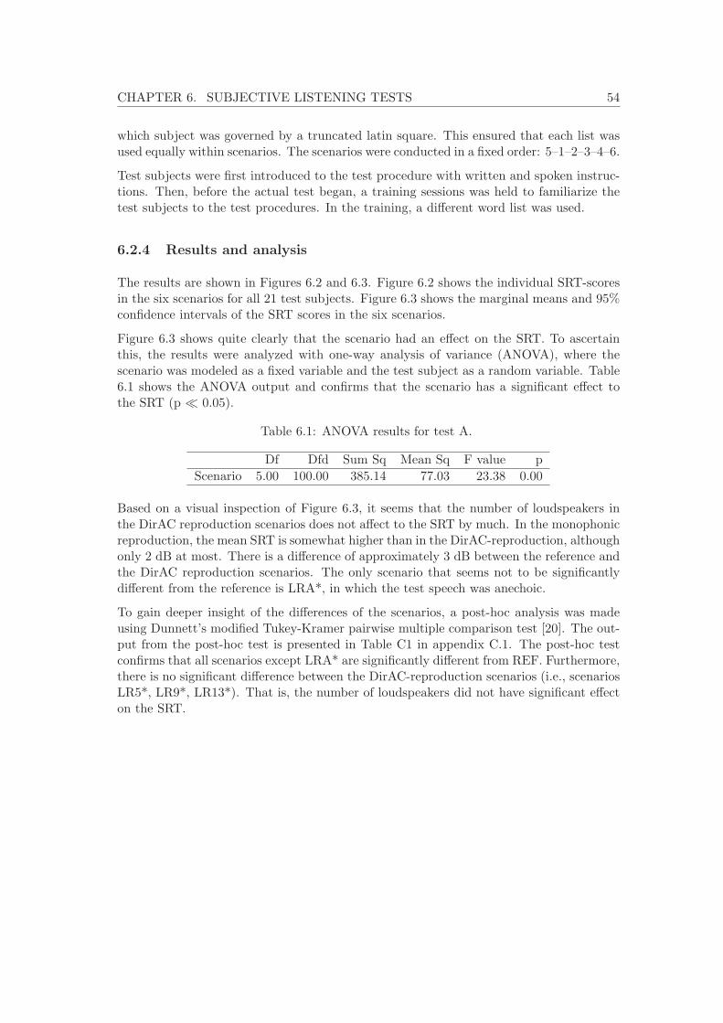
CHAPTER 6. SUBJECTIVE LISTENING TESTS 54
which subject was governed by a truncated latin square. This ensured that each list wasused equally within scenarios. The scenarios were conducted in a fixed order: 5–1–2–3–4–6.
Test subjects were first introduced to the test procedure with written and spoken instruc-tions. Then, before the actual test began, a training sessions was held to familiarize thetest subjects to the test procedures. In the training, a different word list was used.
6.2.4 Results and analysis
The results are shown in Figures 6.2 and 6.3. Figure 6.2 shows the individual SRT-scoresin the six scenarios for all 21 test subjects. Figure 6.3 shows the marginal means and 95%confidence intervals of the SRT scores in the six scenarios.
Figure 6.3 shows quite clearly that the scenario had an effect on the SRT. To ascertainthis, the results were analyzed with one-way analysis of variance (ANOVA), where thescenario was modeled as a fixed variable and the test subject as a random variable. Table6.1 shows the ANOVA output and confirms that the scenario has a significant effect tothe SRT (p � 0.05).
Table 6.1: ANOVA results for test A.
Df Dfd Sum Sq Mean Sq F value p
Scenario 5.00 100.00 385.14 77.03 23.38 0.00
Based on a visual inspection of Figure 6.3, it seems that the number of loudspeakers inthe DirAC reproduction scenarios does not affect to the SRT by much. In the monophonicreproduction, the mean SRT is somewhat higher than in the DirAC-reproduction, althoughonly 2 dB at most. There is a difference of approximately 3 dB between the reference andthe DirAC reproduction scenarios. The only scenario that seems not to be significantlydifferent from the reference is LRA*, in which the test speech was anechoic.
To gain deeper insight of the differences of the scenarios, a post-hoc analysis was madeusing Dunnett’s modified Tukey-Kramer pairwise multiple comparison test [20]. The out-put from the post-hoc test is presented in Table C1 in appendix C.1. The post-hoc testconfirms that all scenarios except LRA* are significantly different from REF. Furthermore,there is no significant difference between the DirAC-reproduction scenarios (i.e., scenariosLR5*, LR9*, LR13*). That is, the number of loudspeakers did not have significant effecton the SRT.
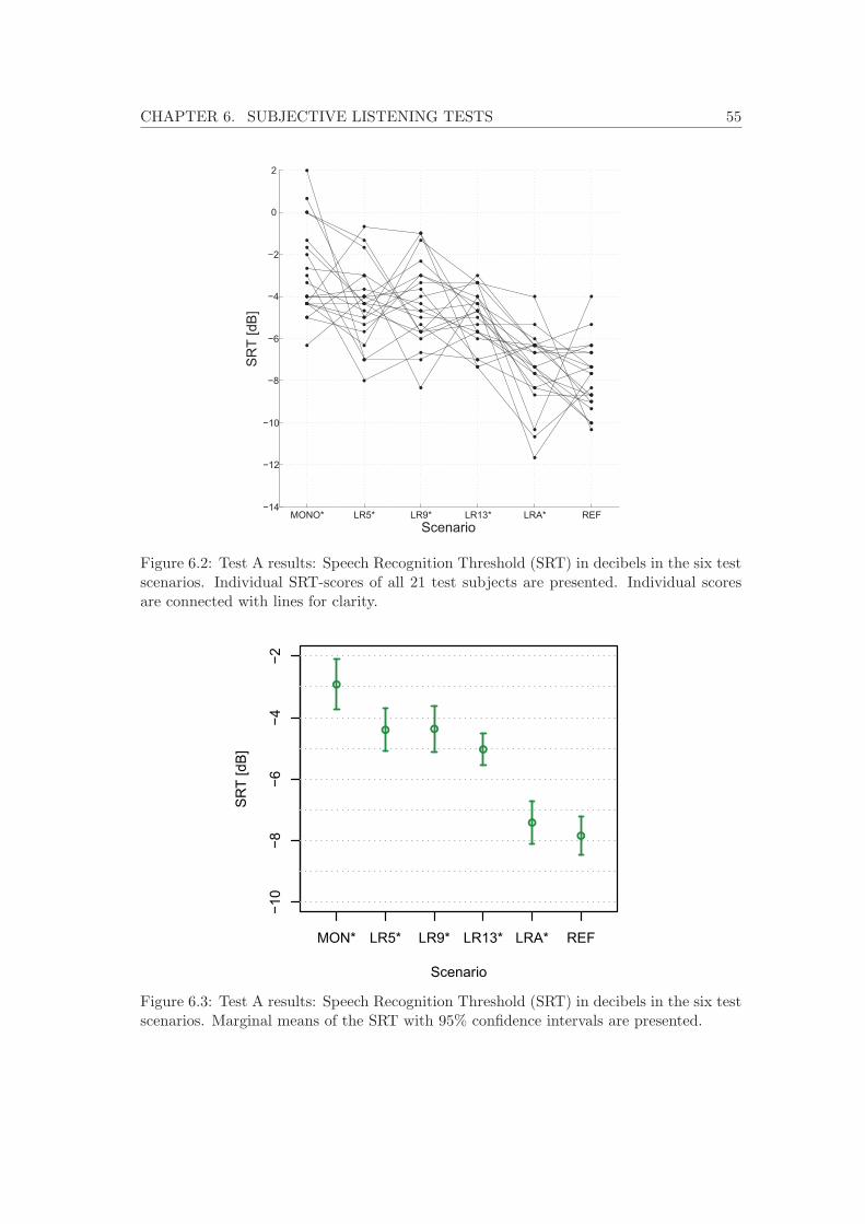
CHAPTER 6. SUBJECTIVE LISTENING TESTS 55
MONO* LR5* LR9* LR13* LRA* REF−14
−12
−10
−8
−6
−4
−2
0
2
SR
T [d
B]
Scenario
Figure 6.2: Test A results: Speech Recognition Threshold (SRT) in decibels in the six testscenarios. Individual SRT-scores of all 21 test subjects are presented. Individual scoresare connected with lines for clarity.
−10
−8−6
−4−2
Scenario
SR
T [d
B]
MON* LR5* LR9* LR13* LRA* REF
●
● ●
●
●
●
Figure 6.3: Test A results: Speech Recognition Threshold (SRT) in decibels in the six testscenarios. Marginal means of the SRT with 95% confidence intervals are presented.

CHAPTER 6. SUBJECTIVE LISTENING TESTS 56
6.3 Test B
6.3.1 Introduction
For each test subject, SRT was measured in the following scenarios.
1. MONO - Mono reproduction in the listening room prototype
2. LR5 - DirAC-reproduction in the listening room prototype with five loudspeakers
3. LR9 - DirAC-reproduction in the listening room prototype with nine loudspeakers
4. AC5 - DirAC-reproduction in the anechoic prototype with five loudspeakers
5. AC9 - DirAC-reproduction in the anechoic prototype with nine loudspeakers
6. REF - The reference environment
The listening room scenarios (MONO, LR5, and LR9) were similar to respective scenariosin test A (MONO*, LR5*, and LR9*), with the exception that now all the loudspeakerswere positioned at a distance of 1 m from the listening position. The distance of theloudspeakers was decreased to increase the direct-to-reverberant ratio at the listeningposition, as this was assumed to decrease the error in SRT for these scenarios. Theloudspeakers were calibrated to that positioning with the dedicated calibration software bythe loudspeaker manufacturer. Scenarios AC5 and AC9 were identical to the LR5 and LR9,respectively, but conducted in the anechoic prototype setup. In these scenarios, listeningposition was in the middle of the loudspeaker array equidistant of the loudspeakers.
Unlike in test A, the test subjects in test B were positioned facing to azimuth -60◦, thatis, their right ear directed towards the front loudspeaker, which is in azimuth 0◦. This wasdone to maximize BILD. At the presentation azimuth of ±60◦, BILD is approximately 2.5dB higher compared to presentation azimuth of 0◦ [8]. Thus, this positioning was assumedto give the most binaural benefit in the test and thereby be the most effective in revealingdifferences between the scenarios. Additionally, this positioning was assumed to maximizethe test subjects’ performance in the test. Namely, with uncorrelated enveloping noise,the best intelligibility is achieved when the desired sound is presented from the azimuth±60◦ [8]. Indeed, people sometimes turn their head to this angle when trying to listen ininterfering noise. This behavior was noticed with some test subjects in test A. Thereby,as the test subjects were now initially in the tilted position, more consistent results wereassumed.
6.3.2 Test subjects
Eighteen test subjects with normal hearing thresholds participated in test B. The testsubjects, 16 of which males and two females, were all native Finnish speakers (age between23–42). The test subjects were volunteers and were not given any reward for participatingin the test.

CHAPTER 6. SUBJECTIVE LISTENING TESTS 57
6.3.3 Test procedures
The test procedures in test B were identical with the procedures in test A with the followingtwo exceptions. First, the initial SNR of the track was 0 dB for all scenarios. Second, theorder in which the scenarios were conducted was governed with a latin square to avoidlearning effects.
6.3.4 Results and analysis
The results are shown in Figures 6.4 and 6.5. Figure 6.4 shows the individual SRT-scoresin the six scenarios for all 18 test subjects. Figure 6.5 shows the marginal means and 95%confidence intervals of the SRT scores in the six scenarios.
Figure 6.5 shows quite clearly that the scenario had an effect to the SRT. To ascertainthis, the results were analyzed with one-way analysis of variance (ANOVA), where thescenario was modeled as a fixed variable and the test subject as a random variable. Table6.2 shows the ANOVA output and confirms that the scenario has a significant effect tothe SRT (p � 0.05).
Table 6.2: ANOVA results for test B.
Df Dfd Sum Sq Mean Sq F value p
Scenario 5.00 85.00 295.86 59.17 17.07 0.00
Based on visual inspection of Figure 6.5, seems that both the amount of room reverberationand the number of loudspeakers have some effect on the SRT. However, the effect is quitesubtle at least in the DirAC-reproduction scenarios. In the monophonic reproduction, abias of 5 dB can be seen compared to the reference.
To gain deeper insight of the differences of the scenarios, a post-hoc analysis was madeusing Dunnett’s modified Tukey-Kramer pairwise multiple comparison test [20]. The out-put from the post-hoc test is presented in Table C2 in appendix C.2. According to thepost-hoc test, the MONO-scenario is significantly different from all the others. ScenariosAC9, AC5, and LR9 have no significant difference compared to REF. Without the scenarioLR5 there would be two distinct subgroups (MONO and the others), but scenario LR5 issignificantly different not only from MONO, but also from AC9 and REF.

CHAPTER 6. SUBJECTIVE LISTENING TESTS 58
MONO LR5 LR9 MCC5 MCC9 REF−14
−12
−10
−8
−6
−4
−2
0
2
SR
T [d
B]
Scenario
Figure 6.4: Test B results: Speech Recognition Threshold (SRT) in decibels in the six testscenarios. Individual SRT-scores of all 18 test subjects are presented. Individual scoresare connected with lines for clarity.
−10
−8−6
−4−2
Scenario
SR
T [d
B]
MONO LR5 LR9 AC5 AC9 REF
Figure 6.5: Test B results: Speech Recognition Threshold (SRT) in decibels in the six testscenarios. Marginal means of the SRT with 95% confidence intervals are presented.
CHAPTER 6. SUBJECTIVE LISTENING TESTS 59
6.4 Test C
6.4.1 Introduction
The aim in test C was to repeat test B using hearing instrument users as test subjects.In this test, for each subject, SRT was measured in the same six scenarios as in test B,described in Section 6.3.1. The only difference in the scenarios compared to test B was thatnow the test subjects were positioned facing to the front loudspeaker. This positioningwas assumed to give generally the best – and also the most uniform – speech intelligibilityamong the test subjects in test C. The hearing-impaired test subjects were assumed tohave negligible benefit from the increased BILD in the -60◦ position. Additionally, thetilted positioning would probably have given more benefit to test subjects with their betterear on the right. Using the the forward-facing positioning in test C was assumed to retainthe comparability of tests B and C, while now both test subjects groups were positionedfor the best and most uniform hearing performance in the test.
6.4.2 Test subjects
Eight test subjects participated in test C. The test subjects were all females and nativeFinnish speakers of the age 36 to 62. The test subjects were volunteers and they werepaid an honorarium of 15 e for participating in the test. All test subjects had bilateralhearing loss which was being aided unilaterally or bilaterally by a hearing aid, cochlearimplant, or both. Table 6.3 summarizes the hearing abilities of the test subjects.
Table 6.3: Test subjects in test C: hearing loss types and hearing instrument types. HArefers to hearing aid and CI to cochlear implant. Test subject RL had a wireless mi-crophone in her almost-deaf right ear, which was connected to the aid in the left ear.
Left ear Right ear
ID Hearing loss type Instrument Hearing loss type Instrument
RN sensorineural CI sensorineural HAMH sensorineural CI sensorineural noneSH deaf none sensorineural HASS sensorineural CI sensorineural HASK sensorineural CI sensorineural HAJV deaf none sensorineural CIRL sensorineural microphone sensorineural HARP sensorineural none sensorineural CI
6.4.3 Test procedures
Test C consisted of two consecutive parts. Both parts consisted of the same SRT-procedureas did one test round in test B, with the following changes.
The first part was considered adaptation and second part was the actual test. The testsubjects were not informed about this. In the first part, the masker level was 65 dB SPL.

CHAPTER 6. SUBJECTIVE LISTENING TESTS 60
Initial SNR of the adaptive track was 10 dB and the SNR was limited between -60 and+20 dB. During the first part, the adaptive track was carefully monitored. If it seemedthat the maximum SNR of +20 dB was not adequate for the test subject, the masker levelwas reduced to 55 dB SPL and the initial SNR was increased to 20 dB for the second part.This procedure made sure that in the second part, as the actual data was collected, noceiling effects were present and the masker level was at is maximum while the maximumSPL in the test room was limited to 85 dB SPL at all times.
Before the test began, the test subjects were asked to set their hearing devices to suchsetting that they would generally use in communication situations with background noise.They were also asked to adjust the gain of their hearing instruments to desired level duringthe training session.
6.4.4 Results and analysis
The results are shown in Figures 6.6 and 6.7. Figure 6.6 shows the individual SRT-scoresin the six scenarios for all the eight test subjects. Figure 6.7 shows the marginal meansand 95% confidence intervals of the SRT scores in the six scenarios. The masker level was65 dB SPL for all test subjects except test subject SK, for whom the masker level wasreduced to 55 dB SPL to avoid ceiling effects.
Figure 6.7 shows that although the marginal means deviate up to 4 dB between scenarios,the 95% confidence intervals are clearly overlapping. According to visual inspection of thefigure, seems that the scenario does not have significant effect on the SRT. To ascertainthis, the results were analyzed with one-way analysis of variance (ANOVA), where thescenario was modeled as a fixed variable and the test subject as a random variable. Table6.4 shows the ANOVA output and confirms that the scenario had no significant effect tothe SRT (p > 0.05).
Table 6.4: ANOVA results for test C.
Df Dfd Sum Sq Mean Sq F value p
Scenario 5.00 35.00 80.65 16.13 1.70 0.16

CHAPTER 6. SUBJECTIVE LISTENING TESTS 61
MONO LR5 LR9 MCC5 MCC9 REF−10
−5
0
5
10
15
20
25
SR
T [d
B]
Scenario
RNMHSHSSSKJVRLRP
Figure 6.6: Test C results: Speech Recognition Threshold (SRT) in decibels in the six testscenarios. Individual SRT-scores of all eight test subjects are presented. Individual scoresare connected with lines for clarity.
24
68
1012
1416
Scenario
SR
T [d
B]
MONO LR5 LR9 AC5 AC9 REF
Figure 6.7: Test C results: Speech Recognition Threshold (SRT) in decibels in the six testscenarios. Marginal means of the SRT with 95% confidence intervals are presented.

CHAPTER 6. SUBJECTIVE LISTENING TESTS 62
6.5 Comparison of the results in tests A, B, and C
6.5.1 On the comparability of the results
Although the general test procedures were the same in all three tests, there were someminor differences. The effect of these differences must be understood in order to comparedthe results between tests. The differences in the initial SNR of the adaptive track verylikely had no significant effect, because of the adaptive testing method. The test subjectorientation (facing 0◦ in test A and C, facing -60◦ in test B) probably had an effect onthe test subjects’ hearing performance, but the effect was constant through the scenarios.Thus, when using the SRT-scores from a given test relative to the reference scenario ofthe same test, the results are comparable between the three tests.
6.5.2 The effect of direct-to-reverberant ratio in the listening position
Figure 6.8 shows a comparison of all the six scenarios where five or nine loudspeakerswere used. The mean errors in SRT compared to the reference scenario of respective testare presented. The mean error of a scenario was calculated as the mean of the individualSRTs that were each normalized to the individual SRT measured in the reference scenario.Figure 6.8 shows that increasing the DRR in the listening position decreases the speechintelligibility and thus increases the error in the SRT.
−20
24
6
Scenario
Err
or in
SR
T [d
B]
LR5* LR5 AC5 LR9* LR9 AC9
● ●
Figure 6.8: Comparison of the results in tests A and B: the effect of direct-to-reverberantratio with five and nine loudspeakers. Marginal means of the errors in SRT compared tothe respective reference scenario are presented with 95% confidence intervals. Data fromtest A in green circles and data from test B in blue squares.
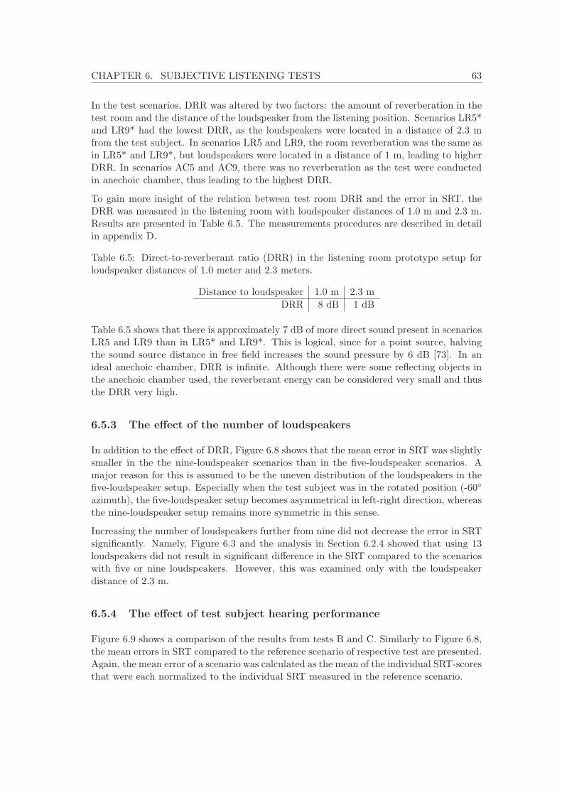
CHAPTER 6. SUBJECTIVE LISTENING TESTS 63
In the test scenarios, DRR was altered by two factors: the amount of reverberation in thetest room and the distance of the loudspeaker from the listening position. Scenarios LR5*and LR9* had the lowest DRR, as the loudspeakers were located in a distance of 2.3 mfrom the test subject. In scenarios LR5 and LR9, the room reverberation was the same asin LR5* and LR9*, but loudspeakers were located in a distance of 1 m, leading to higherDRR. In scenarios AC5 and AC9, there was no reverberation as the test were conductedin anechoic chamber, thus leading to the highest DRR.
To gain more insight of the relation between test room DRR and the error in SRT, theDRR was measured in the listening room with loudspeaker distances of 1.0 m and 2.3 m.Results are presented in Table 6.5. The measurements procedures are described in detailin appendix D.
Table 6.5: Direct-to-reverberant ratio (DRR) in the listening room prototype setup forloudspeaker distances of 1.0 meter and 2.3 meters.
Distance to loudspeaker 1.0 m 2.3 m
DRR 8 dB 1 dB
Table 6.5 shows that there is approximately 7 dB of more direct sound present in scenariosLR5 and LR9 than in LR5* and LR9*. This is logical, since for a point source, halvingthe sound source distance in free field increases the sound pressure by 6 dB [73]. In anideal anechoic chamber, DRR is infinite. Although there were some reflecting objects inthe anechoic chamber used, the reverberant energy can be considered very small and thusthe DRR very high.
6.5.3 The effect of the number of loudspeakers
In addition to the effect of DRR, Figure 6.8 shows that the mean error in SRT was slightlysmaller in the the nine-loudspeaker scenarios than in the five-loudspeaker scenarios. Amajor reason for this is assumed to be the uneven distribution of the loudspeakers in thefive-loudspeaker setup. Especially when the test subject was in the rotated position (-60◦
azimuth), the five-loudspeaker setup becomes asymmetrical in left-right direction, whereasthe nine-loudspeaker setup remains more symmetric in this sense.
Increasing the number of loudspeakers further from nine did not decrease the error in SRTsignificantly. Namely, Figure 6.3 and the analysis in Section 6.2.4 showed that using 13loudspeakers did not result in significant difference in the SRT compared to the scenarioswith five or nine loudspeakers. However, this was examined only with the loudspeakerdistance of 2.3 m.
6.5.4 The effect of test subject hearing performance
Figure 6.9 shows a comparison of the results from tests B and C. Similarly to Figure 6.8,the mean errors in SRT compared to the reference scenario of respective test are presented.Again, the mean error of a scenario was calculated as the mean of the individual SRT-scoresthat were each normalized to the individual SRT measured in the reference scenario.

CHAPTER 6. SUBJECTIVE LISTENING TESTS 64
Although normal hearing test subjects had the best intelligibility in the reference scenario,it seems that for the hearing instrument users the intelligibility is slightly better in theDirAC-reproduction scenarios. However, in the test subjects group of test C the differencesare quite small and the confidence intervals quite large. In both groups, the MONO-scenario produces the worst intelligibility and the largest error compared to the reference.All in all, there was no significant differences between any scenarios in test C.
−4−2
02
46
Scenario
Err
or in
SR
T [d
B]
MONO LR5 LR9 AC5 AC9
Figure 6.9: Comparison of the results in tests B and C: the effect of the test subjecthearing performance. Marginal means of the errors in SRT compared to the respectivereference scenario are presented with 95% confidence intervals. Data from test B in bluesquares and data from test C in red crosses.
6.6 Reliability of the results
The reliability of the results can be considered generally good. There is still a few possiblesources of error.
Most importantly, there was considerable amount of noise in the data, as could be seenfrom the individual SRT-scores from all tests (Figures 6.2, 6.4, and 6.6). That is, notall individual tracks clearly followed the overall trend. Visual inspection of the adaptivetracks in the tests revealed that not always clear adaptation happened: in some cases, thetrack wandered up and down aimlessly. There are several facts related to the word liststhat could have caused this. First, the word lists used are considered a bit old-fashionedby the author. That is, some of the words were uncommon, of old style, or ones that canbe considered colloquial. These findings were also agreed by many of the test subjectsduring informal discussion after the test, in which the test subjects were asked: ”how didyou like the test speech material?”. It is obvious that the word lists should consist onlyof words which everybody knows and understands, and now there was a few exceptions
CHAPTER 6. SUBJECTIVE LISTENING TESTS 65
degrading the balance of the lists. Second, the speech corpus was quite small. The noisein the results could probably have been decreased by using a larger corpus. Namely, witha larger number of inter-compatible word lists each scenario could have been conductedwith several interleaved lists. A longer word lists could also have improved the adaptation.In tests A and B an adequate number of test subjects was used to average the noise outof the data. In test C the number of test subjects was unfortunately lower, but probablyfair enough for the analysis required.
Another issue is the comparability of the SNRs. The SNR between masker and test speechin the listening position was carefully measured using the same method for all scenarios.This ensured that the results are comparable between scenarios. Small variation to theeffective SNR has probably been caused by the fact that test subjects were not deniedto move their head during the test. Still, based on visual observations during the testprocedures, the effect of this is quite small.
In contrast, there may be error in the absolute value of the SNR. This is due to the difficultyof defining the SNR between a masker and reverberant speech, or to be precise, of definingwhat part of the speech is actually the desired signal. That is, in reverberant speech,the direct sound and early reflections are desired and increasing their level increases theintelligibility. On the other hand, late reflections and excessive reverberation can insteaddecrease the intelligibility. However, in these tests, the absolute value of SNR is not ofinterest: the test method is based on relative differences in the SRT obtained in differentscenarios. Thus, in these tests, all energy of the test speech was regarded as the desiredsignal.
In test A, the fixed order of scenarios could have caused learning effects, if listening tothe first scenarios gained the test subjects performance in the last scenarios. However,this did not probably have significant effect to the results. First reason for this is thatthe test procedures represented nothing more than communication in noise, which is quitean everyday-task. Secondly, different word lists were used in different scenarios, and theywere randomized between scenarios. Thus, benefiting from memorizing the words was notpossible. Regardless, in tests B and C, the scenario order was balanced with a latin squareto avoid order-related effects.

Chapter 7
Discussion
This chapter concludes and interprets the outcome of the listening tests and evaluates theproposed DirAC-based sound-field audiometry system. Suggestions are made for a clinicalimplementation of the concept, and possible future work is discussed.
7.1 Outcome of the listening tests
The outcomes of the listening tests reported in Chapter 6 can be concluded as follows.First, both the number of loudspeakers and the direct-to-reverberant ratio has an ef-fect on the SRT. When nine loudspeakers were used, there was no significant differencebetween the SRTs obtained in the reference environment and the corresponding DirAC-reproduction in the anechoic prototype setup or the listening room prototype setup withone-meter loudspeaker distance. Decreasing the DRR decreased the SRT-scores and thusincreased the error compared to the reference environment. Using an asymmetrical five-loudspeaker setup led to higher error compared to a nine-loudspeaker setup, but was stillfound to be valid in anechoic conditions. Second, compared to monophonic reproduction,the DirAC-reproduction resulted in smaller error in SRT. This motivates the use of severalloudspeakers instead of one. Finally, the test subject group consisting of hearing instru-ment users did not perform in significantly different ways in the tested scenarios. Thisconfirmed that the psychoacoustic assumptions of DirAC were valid also with listenerswith non-normal hearing.
7.2 Evaluation of the DirAC-based SFA system
7.2.1 Validity
The outcomes of the listening tests can be interpreted as follows. First, the proposedconcept of DirAC-based sound-field audiometry is valid at least in terms of speech intelli-gibility assessments. This is due to no significant indifferences in the SRTs measured in areference ”real life” scenario and its DirAC-reproduction equivalent. This validity is metwhen using a symmetrical setup of nine loudspeakers in a room with a DRR of 8 dB orhigher in the listening position. The validity is ensured only with the particular audio
66
CHAPTER 7. DISCUSSION 67
used in the listening tests. Thus, no explicit conclusion can be made on the validity whenother sound scenes are reproduced.
Valid results might be achievable with somewhat looser requirements, for example witha lower number of loudspeaker – given that the loudspeakers are evenly placed – or witha lower DRR. However, a conventional 5.1-setup was found to be insufficient even withDRR of 8 dB as well as was DRR of 1 dB with nine loudspeakers.
7.2.2 Advantages and drawbacks
Compared to existing methods for sound-field audiometry, the proposed method has sev-eral clear advantages. First, no more than nine loudspeakers in the horizontal plane areneeded for adequate reproduction concerning speech intelligibility assessments in realisticsound scenes. Second, due to the use of parametric audio coding, the number of loud-speakers and their positioning are arbitrary as long as the minimum requirements aremet. Third, the system is capable of reproducing real sound scenes including the as-sociated room acoustics, in which anechoic test speech material can be augmented. Incontrast, many of the current methods are based on simulations or use synthesized audiomaterial. Using real recorded environments enables more realistic testing. Finally, thesystem is modular as different background sound scenes, room acoustics, and anechoicspeech corpuses can be combined freely.
The proposed method has also some drawbacks. The system must be calibrated carefullyto obtain reliable results. That is, the SPL of the masker and test speech must be measuredand adjusted carefully to ensure the correct SNR in the test. This is somewhat a commondrawback in all sound-field audiometry applications, but is emphasized when real recordedaudio is used.
7.2.3 Suggestions for clinical implementations
Suggestions for a clinical DirAC-based SFA setup specifications are as follows.
The preferred arrangement of loudspeakers is a somewhat even and symmetrical arrange-ment in the horizontal plane at the ear-level of the listener. Nine loudspeakers are recom-mended.
The test room should have a relatively low reverberation time. Generally, the lower thebetter. The listening room used in the test of this thesis is an example of a suitable testroom (see Section 5.3.3 for specifications). In that room, the loudspeaker distance of 1meter resulted in a DRR of 8 dB. Following a listening room recommendation (such asITU-R BS.1116 [35]) or the quasi-free sound field conditions [33] would be advantageousin the long run. That is, anchoring the requirements to an existing standard would makeit easy to build new setups and maintain the comparability between them. However, themost important factor is the DRR. The test room and loudspeaker distance from listeningposition should be designed so that a DRR of 8 dB is achieved in the listening position.Preferably, DRR measurements should be done to validate the room for this purpose.Loudspeaker distance of 1 m is suitable. Distances below this are problematic, while thecloser the loudspeakers are, the bigger is the relative change in the loudness when head
CHAPTER 7. DISCUSSION 68
is moved. On the other hand, with much higher loudspeaker distances it may be hard toachieve a high enough DRR.
The audio material used should be selected depending on what kind of situations andscenarios are wanted to be tested. In choosing the masker a compromise is made betweenthe realism of the scene and reliability of the test. The speech corpus to be used should belarge enough and have equal difficulty thorough the test. All audio material used should behigh-pass filtered with a cut-off frequency equal and higher than the Schroeder frequencyof the test room to prevent the effect of room modes.
When implementing the proposed SFA setup in a clinic, the SNR between masker and testspeech must be defined carefully. This is essential if results are wanted to be comparable forexample between different clinics. On the other hand, when conducting relative measures,such as functional gain of a hearing instrument or test similar to which was done in thisthesis, the absolute SNR needs not the be strictly defined. That is, in these cases the erroris subtracted in the comparison. According to [8], the energy in the first 80 ms could beregarded as the desirable sound and the energy after that as the undesired sound. Thiscould be one approach to use for dividing a highly-reverberated test speech to actual signalenergy and masker energy. However, the extent in which the reverberant sound acts as amasker should be carefully analyzed. That is, if a two-syllable test word is used, a three-second reverberation decay is mostly present after the word has ended and is obviously notmasking anymore. When using sentence material, the situation can be somewhat differentas the reverberation of previous words mask the following ones.
7.3 Suggestions for further work
The validity of the concept with some different masker and test speech material is unsure.Thus, one aim for further research could be to repeat the listening tests of this thesis withsome other reference scene. The reference sound scene used in the tests of this thesis hadrelatively low reverberation. Using a scene with higher reverberance might have some effecton the validity of the system. A guess by the author is that using such highly reverberantreference scene would probably loosen the DRR-criteria of the test room. Namely, in thiscase the additional room effect applied by the test room would be smaller compared to theoriginal reverberation and thus have smaller effect on the speech intelligibility. Also, theuse of sentence test speech material together with a percent-intelligibility test procedurecould be considered. In that case, the masker stationarity criterion might not be as strictas when using single words and a SRT procedure.
Only speech intelligibility assessments were discussed in this thesis. However, the con-cept of DirAC-based sound-field audiometry might be extendable to other audiometricmeasurements as well, but these applications should be validated with listening tests de-pending on motivation. Possible applications could be such as hearing-based orientationtasks in reproduced sound scenes.
Adding a visual display to the system would add more realism. This would allow thevisual cues that are naturally present in real environments (e.g., a change to lip-read),which would bring the results even closer to the real-life performance. This could be espe-cially useful when assessing the overall communication performance of hearing-impairedindividuals, while they may gain significant benefit from visual cues. Adding a visual
CHAPTER 7. DISCUSSION 69
display could further broaden the application area and enable for example attention testsin a virtual classroom.
Future work could also include implementing the DirAC-based SFA system as a standalonesoftware for the use of healthcare. In this case, capturing a set of suitable sound sceneswould be also required. For the system to be accepted for diagnostic use, a prototypesetup should be built in a clinic and further validation done with different sound scenesand larger number of test subjects. This could probably be implemented most efficientlyin a multidisciplinary project involving both physicians and engineers.
Chapter 8
Conclusion
This thesis investigated the use of a parametric spatial audio reproduction technique calledDirectional Audio Coding in the field of hearing diagnostics. The motivation for this re-search was given in Chapter 1. The theory part, consisting of Chapters 2–4, exploredthe background of the topic: these chapters discussed the principles of sound and hear-ing, spatial audio technology, and technical audiology with an emphasis on sound-fieldaudiometry.
In the experimental part, consisting of Chapters 5–7, the concept of a sound-field audiom-etry system based on Directional Audio Coding was motivated, designed, and validated. Aprototype setup of the system was built and a MATLAB-software was written for testingthe concept. Additionally, a reference sound installation representing a real environmentwas built for comparison. The concept was validated with listening tests using normally-hearing individuals and users of hearing aid and/or cochlear implant as the test subjects.The listening tests revealed that with an adequate number of loudspeakers and adequatelycontrolled acoustics in the test room, the same speech intelligibility could be achieved inthe reproduced scene as in the reference scene. Based on these findings, suggestions weremade for a clinical implementation of the system.
The proposed method offers a platform for various audiometric tests in real sound sceneswith external speech material augmented to the associated room acoustics. The proposedmethod is more compact and flexible than most of the existing methods in terms of systemmodularity and the loudspeaker setup needed. Consequently, the proposed method couldbe easily applied to clinical purposes.
70
Bibliography
[1] Ahonen, J., and Pulkki, V. Speech intelligibility in teleconference application ofdirectional audio coding. In AES 40th conference on Spatial Audio (2010).
[2] Ahonen, J., Sivonen, V., and Pulkki, V. Nonlinear time-frequency processingapplied to bilateral aided hearing. In Proceedings of Forum Acusticum (2011).
[3] Aronoff, J. M., soo Yoon, Y., Freed, D. J., Vermiglio, A. J., Pal, I., and
Soli, S. D. The use of interaural time and level difference cues by bilateral cochlearimplant users. Journal of Acoustical Society of America 127, 3 (2010).
[4] Arweiler, I. Processing of spatial sounds in the impaired auditory system. PhDthesis, Technical University of Denmark, 2011.
[5] Barron, M. Auditorium acoustics and architectural design. E et F Spon, 1998.
[6] Bartels, H., Staal, M. J., and Albers, F. W. J. Tinnitus and neural plasticityof the brain. Otology and Neurotology 28, 2 (2007), 178–184.
[7] Berkhout, A. J. A holographic approach to acoustic control. Journal of AudioEngineering Society 36, 12 (1988), 977–995.
[8] Blauert, J. Spatial Hearing. The MIT Press, 1997.
[9] Bolia, R. S., Nelson, W. T., and Ericson, M. A. A speech corpus for multitalkercommunications research. Journal of Acoustical Society of America 107, 2 (2000).
[10] Bronkhorst, A. W. The cocktail party phenomenon: A review of research onspeech intelligibility in multiple-talker conditions. Acta acustica 86 (2000), 117–128.
[11] Carhart, C. R. Monitored live-voice as a test of auditory acuity. Journal ofAcoustical Society of America 17, 4 (1946), 339–349.
[12] Chaiklin, J. B., and Ventry, I. M. Spondee threshold measurement: A com-parison of 2- and 5-dB methods. Journal of Speech and hearing disorders 29 (1964),47–59.
[13] Cherry, E. C. Some experiments on the recognition of speech, with one and withtwo ears. Journal of Acoustical Society of America 25, 5 (1953).
[14] Cochlear Ltd. Product website. Cited 28.7.2011. http://www.cochlear.com/au/hearing-loss-teatments/cochlear-implants-adults.
71
BIBLIOGRAPHY 72
[15] Compton-Conley, C. L., Neuman, A. C., Killion, M. C., and Levitt, H.
Performance of directional microphones for hearing aids: Real-world versus simula-tion. Journal of american academy of audiology 15 (2004), 440–455.
[16] Davis, D., and Patronis, E. Sound system engineering. Focal press, 2006.
[17] DELTA Technical-Audiological Laboratory. Guidelines for the set-up andcalibration of equipment employed in free-field audiometry, 2002.
[18] Denis, B. et. al. An international comparison of long-term average speech spectra.Journal of Acoustical Society of America 96, 4 (1994), 2108–2120.
[19] Dillon, H., and Walker, G. Comparison of stimuli used in sound field audiometrictesting. Journal of Acoustical Society of America 71, 1 (1982), 161–172.
[20] Dunnett, C. W. Pairwise multiple comparisons in the unequal variance case. Jour-nal of the American Statistical Association 75, 372 (1980).
[21] Durlach, N. I., Mason, C. R., Kidd Jr., G., Arbogast, T. L., Coldburn,
H. S., and Shinn-Cunningham, B. G. Note on informational masking. Journal ofAcoustical Society of America 113, 6 (2003), 2984–2987.
[22] EU Work Group on Genetics of Hearing Impairment. Infoletter 2. 1996.
[23] Fasti, H., and Seeber, B. U. Localization cues with bilateral cochlear implants.Journal of Acoustical Society of America 123 (2008), 1030–1042.
[24] Favrot, S., and Buchholz, J. M. Lora: A loudspeaker-based room auralizationsystem. Acta acustica 96 (2010), 364–375.
[25] Gerzon, M. A. The design of precisely coincident microphone arrays for stereo andsurround sound. In 50th AES Convention, London, UK (1975).
[26] Gerzon, M. A. Ambisonics in multichannel broadcastingand video. Journal ofAudio Engineering Society 33, 11 (1985), 859–871.
[27] Hallgren, M., Larsby, B., and Arlinger, S. A Swedish version of the hearingin noise test (HINT) for measurement of speech recognition. International Journal ofAudiology 45 (2006), 227–237.
[28] Hornsby, B. W., Ricketts, T. A., and Johnson, E. E. The effects of speech andspeechlike maskers on unaided and aided speech recognition in persons with hearingloss. Journal of the american academy of audiology (2006).
[29] Humphrey, R. Playrec website. Cited 20.1.2012. http://oticon.com/Consumers/Products/Hearing%20aids/Styles%20and%20colours.aspx.
[30] ISO 3382-2:2008. Acoustics standard. Measurement of room acoustic parameters.Part 2: Reverberation time in ordinary rooms.
[31] ISO 389-1:1998. Acoustics standard. Reference zero for the calibration of audiomet-ric equipment - Part 1: Reference equivalent threshold sound pressure levels for puretones and supra-aural earphones.
[32] ISO 8253-1:2010. Acoustics standard. Audiometric testing methods. Part 1: Pure-tone air and bone conduction audiometry.

BIBLIOGRAPHY 73
[33] ISO 8253-2:2009. Acoustics standard. Audiometric testing methods. Part 2: Soundfield audiometry with pure-tone and narrow-band test signals.
[34] ISO 8253-3:1996. Acoustics standard. Audiometric testing methods. Part 3: Speechaudiometry.
[35] ITU-R BS.1116-1. Recommendation. Methods for subjective assessment of smallimpairments in audio systems including multichannel sound systems.
[36] ITU-R BS.775-1. Recommendation. Multichannel stereophonic sound system withand without accompanying picture.
[37] Jauhiainen, T. An Experimental Study of the Auditory Perception of Isolated Bi-syllable Finnish Words. PhD thesis, University of Helsinki, 1974.
[38] Jauhiainen, T. Kuulo ja viestinta. Yliopistopaino, 1995.
[39] Jerger, J., Speaks, C., and Trammell, J. L. A new approach to speech au-diometry. Journal of Speech and hearing disorders 33 (1968), 318–328.
[40] Karjalainen, M. Kommunikaatioakustiikka. Report / Department of signal pro-cessing and acoustics. Helsinki University of technology, 2008.
[41] Karma, P., Nuutinen, J., Pulakka, H., Vilkman, E., Virolainen, E.,
Ylikoski, J., and Ramsay, H. Korva-, nena- ja kurkkutaudit seka foniatrianperusteet. Yliopistopaino, 1999.
[42] Kim, D. O. Hearing Science. College-Hill Press, 1983, ch. Functional roles of theinner- and outer-hair-cell subsystems in the cochlea and brainstream.
[43] Kimball, S. H. Speech audiometry. Medscape Reference (2011).
[44] Klasen, T. J., Moonen, M., van den Bogaert, T., and Wouters, J. Preser-vation of interaural time delay for binaural hearing aids through multi-channel wienerfiltering based noise reduction. In ICASSP, Philadelphia PA, USA (2005).
[45] Laitakari, K. Speech recognition in noise: Development of a computerized test andpreparation of test material. Scandinavian Audiology 25 (1996), 29–34.
[46] Laitakari, K., and Uimonen, S. The finnish speech in noise test for assessingsensorineural hearing loss. Scandinavian Audiology 30, S52 (2001), 165–166.
[47] Leino, T. Long-term average spectrum in screening of voice quality in speech: Un-trained male university students. Journal of Voice 23, 6 (2009), 671–676.
[48] Levitt, H. Transformed up-down methods in psychoacoustics. Journal of AcousticalSociety of America 49, 2B (1971), 467–477.
[49] MacKeith, N. W., and Coles, R. R. A. Binaural advantages in hearing of speech.Journal of Laryngology and otology 85 (1971), 213–232.
[50] Marrone, N., Mason, C. R., and Kidd Jr., G. Tuning in the spatial dimension:Evidence from a masked speech identification task. Journal of Acoustical Society ofAmerica 124, 2 (2008), 1146–1158.
[51] Martin, F. N., and Clark, J. G. Introduction to audiology, 9 ed. Pearson/Allynand Bacon, 2006.

BIBLIOGRAPHY 74
[52] Merimaa, J., Peltonen, T., and Lokki, T. Concert hall impulse responses, Pori,Finland: Reference. Tech. rep., 2005.
[53] Merimaa, J., and Pulkki, V. Spatial impulse response rendering I: Analysis andsynthesis. Journal of Audio Engineering Society 53, 12 (2005), 1115–1127.
[54] Minnaar, P., Breitspecher, C., and Holmberg, M. Simulating complex listen-ing environments in the laboratory for testing hearing aids. In Proceedings of ForumAcusticum (2011).
[55] Møller, A. R. Advances in oto-rhino-laryngology, volume 64: Cochlear and Brain-sterm implants. Karger Publishers, 2006.
[56] Moore, B. C. J. Perceptual consequences of cochlear hearing loss and their impli-cations for the design of hearing aids. Ear and hearing 17 (1996), 133–160.
[57] Mosnier, I., Sterkers, O., Bebear, J.-P., Godey, B., Robier, A., Deguine,
O., Fraysse, B., Bordure, P., Mondain, M., Bouccara, D., Bozorg-
Grayelia, A., Borel, S., Ambert-Dahan, E., and Ferrary, E. Speech perfor-mance and sound localization in a complex noisy environment in bilaterally implantedadult patients. Audiology and Neurotology 14 (2009), 106–114.
[58] Nilsson, M., Soli, S. D., and Sullivan, J. A. Development of the hearing innoise test for the measurement of speech reception thresholds in quiet and in noise.Journal of Acoustical Society of America 95 (1994), 1085–1099.
[59] Nopp, P., Schleich, P., and DA´Haese, P. Sound localization in bilateral usersof MED-EL COMBI 40/40+ cochlear implants. Ear and hearing (2005).
[60] Oticon A/S. Product website. Cited: 28.7.2011. http://oticon.com/Consumers/Products/Hearing%20aids/Styles%20and%20colours.aspx.
[61] Politis, A., and Pulkki, V. Broadband analysis and synthesis for directionalaudio coding using a-format input signals. In 131st AES Convention, New York,USA (2011).
[62] Puder, H. Hearing aids: An overview of the state-of-the-art, challenges, and futuretrends of an interesting audio signal processing application. In Proceedings of the 6thinternational symposium on image an signal procesing and analysis (2009).
[63] Pulkki, V. Virtual sound source positioning using vector base amplitude panning.Journal of Audio Engineering Society 45, 6 (1997).
[64] Pulkki, V. Uniform spreading of amplitude panned virtual sources. In IEEE Work-shop on Applicafions orsignal Processing to Audio and Acouslics (1999).
[65] Pulkki, V. Coloration of amplitude-panned virtual sources. In AES 110th convention(2001).
[66] Pulkki, V. Localization of amplitude-panned virtual sources II: Two- and three-dimensional panning. Journal of Audio Engineering Society 49, 9 (2001).
[67] Pulkki, V. Compensating displacement of amplitude-panned virtual sources. In22nd International Conference: Virtual, Synthetic, and Entertainment Audio (2002).

BIBLIOGRAPHY 75
[68] Pulkki, V. Spatial sound reproduction with directional audio coding. Journal ofAudio Engineering Society 55, 6 (2007), 503–516.
[69] Pulkki, V., and Merimaa, J. Spatial impulse response rendering: A tool forreproducing room acoustics for multi-channel listening. Tech. rep., Helsinki Universityof Technology and Waves Inc.
[70] Revit, L. J., and Schulein, R. B. United states patent no. 7,340,062 b2: Soundreproduction method and apparatus for assessing real-world performance of hearingand hearing aids, 2008.
[71] Revit, L. J., Schulein, R. B., and Julstrom, S. D. Toward accurate assessmentof real-world hearing aid benefit. The Hearing review (2002).
[72] Ricketts, T. Impact of noise source configuration on directional hearing aid benefitand performance. Ear Hear 21 (2000), 194–205.
[73] Rossing, T. D., Moore, F. R., and Wheeler, P. A. The science of sound, 3 ed.Addisong Wesley, 2002.
[74] Rychtarikova, M., van den Bogaert, T., Vermeir, G., and Wouters, J.
Perceptual validation of room acoustic simulation method for sound source localisa-tion and speech intelligibility tests. In Proceedings of Forum Acusticum (2011).
[75] Schleich, P., Nopp, P., and DA´Haese, P. Head shadow, squelch, and summa-tion effects in bilateral users of the MED-EL COMBI 40/40+ cochlear implant. Earand hearing 25 (2004), 197–204.
[76] Schroeder, M. R. New method of measuring reverberation time. Journal of Acous-tical Society of America 37, 3 (1965), 409–412.
[77] Schroeder, M. R. The ”Schroeder frequency” revisited. Journal of AcousticalSociety of America (1995).
[78] Seeber, B. U. Research homepage. Cited 28.7.2011. http://www.acoustics.
bseeber.de/index.html.
[79] Seeber, B. U., Kerber, S., and Hafter, E. R. A system to simulate andreproduce audio-visual environments for spatial hearing research. Hearing Research260 (2010), 1–10.
[80] Siemens. TruEar technology website. Cited 8.3.2012. http://hearing.siemens.
com/ca/01-professional/02-bestsound-technology/02-sound-comfort/
03-optimizing-localization/02-truear/truear.jsp.
[81] Solvang, A. Spectral impairment for two-dimensional higher order ambisonics.Journal of the Audio engineering Society (2008).
[82] Spriet, A., Proudler, I., Moonen, M., and Wouters, J. Adaptive feedbackcancellation in hearing aids with linear prediction of the desired signal. IEEE Trans-actions on signal processing 53, 10 (2005), 3749–3763.
[83] Steinberg, J. C., and Gardner, M. B. The dependence of hearing impairmenton sound intensity. Journal of Acoustical Society of America 9 (1937), 11–23.
BIBLIOGRAPHY 76
[84] University of California San Francisco Benioff Children’s Hospital.Website. Cited 28.7.2011. http://www.ucsfbenioffchildrens.org/treatments/
cochlear_implant/.
[85] Vilkamo, J., Lokki, T., and Pulkki, V. Directional audio coding: Virtualmicrophone-based synthesis and subjective evaluation. Journal of Audio EngineeringSociety 57, 9 (2009).
[86] VU University Medical Center. HearCom project website. Cited 5.7.2011.http://hearcom.eu/prof.html.
[87] VU University Medical Center. HearCom report D-7-2: Specifications of stan-dard speech test/environmental conditions for Europe. 2006.
[88] VU University Medical Center. Hearcom report d-7-3: Specification spatial-hearing test. 2006.
[89] Walker, G., Dillon, H., and Byrne, D. Sound field audiometry: Recommendedstimuli and procedures. Ear and hearing 5, 1 (1984), 13–21.
[90] Warren, R. M. Auditory Perception: A new synthesis. Pergamon press Inc., 1982.
[91] Wenzel, E. M., Arruda, M., Kistler, D. J., and Wightman, F. L. Localiza-tion using non-individualized head-related transfer functions. Journal of AcousticalSociety of America 94, 1 (1993), 111–123.
[92] Yost, W. A. Fundamentals of Hearing - An Introduction. Academic Press, 1994.
[93] Young, H. D., and Freedman, R. A. University Physics, 11 ed. Addison Wesley,2003.
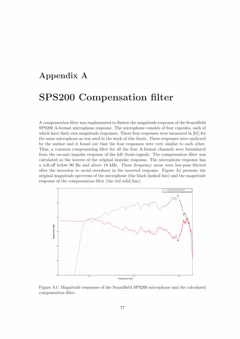
Appendix A
SPS200 Compensation filter
A compensation filter was implemented to flatten the magnitude response of the SoundfieldSPS200 A-format microphone response. The microphone consists of four capsules, each ofwhich have their own magnitude responses. These four responses were measured in [61] forthe same microphone as was used in the work of this thesis. These responses were analyzedby the author and it found out that the four responses were very similar to each other.Thus, a common compensating filter for all the four A-format channels were formulatedfrom the on-axis impulse response of the left–front-capsule. The compensation filter wascalculated as the inverse of the original impulse response. The microphone response hasa roll-off below 90 Hz and above 18 kHz. These frequency areas were low-pass filteredafter the inversion to avoid overshoot in the inverted response. Figure A1 presents theoriginal magnitude spectrum of the microphone (the black dashed line) and the magnituderesponse of the compensation filter (the red solid line).
102
103
104
−20
−15
−10
−5
0
5
10
Frequency [Hz]
Mag
nitu
de [d
B]
SPS200 magnitude responseCompensation filter magnitude response
Figure A1: Magnitude responses of the Soundfield SPS200 microphone and the calculatedcompensation filter.
77
Appendix B
Reverberation time measurementdetails
Reverberation time (RT) was measured in the reference environment and in the listeningroom following the standard ISO 3382 [30]. Interrupted pink noise was used as the excita-tion signal. Total of 12 measurements were done in both rooms, namely in two loudspeakerlocations, each with three microphone locations, and each with two repetitions.
The noise was generated in MATLAB and reproduced with an active loudspeaker (Genelec8030A). Measurements were done with a microphone (B&K, type 4192 capsule and type2669 preamplifier) and a conditioning amplifier (Nexus) connected to a computer (AppleMacbook) via an audio interface (MOTU Traveler mk3).
Analysis was done in MATLAB, with a script utilizing Schroeder backward integration[76]. T30 procedure was used in the analysis. That is, the time for the sound to attenuatefrom -5 dB to -35 dB was analyzed and the respective value for the 60 dB attenuation wascalculated by doubling the RT30 value. The analysis was done in nine octave bands: 63Hz to 8 kHz. The final value of RT in each octave band was calculated as the average ofthe 12 measurements. Finally, an average value for RT was calculated as the average ofthe values of octave bands 500 Hz and 1 kHz.
Measurements from the 31 Hz octave band were not reliable due to the limited frequencyresponse of the loudspeaker used. This octave band was however not of interest in thisthesis, while all audio used in the tests was high-pass filtered with 100 Hz cut-off frequency.
78
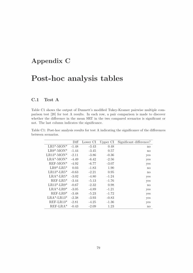
Appendix C
Post-hoc analysis tables
C.1 Test A
Table C1 shows the output of Dunnett’s modified Tukey-Kramer pairwise multiple com-parison test [20] for test A results. In each row, a pair comparison is made to discoverwhether the difference in the mean SRT in the two compared scenarios is significant ornot. The last column indicates the significance.
Table C1: Post-hoc analysis results for test A indicating the significance of the differencesbetween scenarios.
Diff Lower CI Upper CI Significant difference?
LR5*-MON* -1.48 -3.43 0.48 noLR9*-MON* -1.44 -3.45 0.57 noLR13*-MON* -2.11 -3.86 -0.36 yesLRA*-MON* -4.49 -6.42 -2.56 yesREF-MON* -4.92 -6.77 -3.07 yesLR9*-LR5* 0.03 -1.83 1.90 noLR13*-LR5* -0.63 -2.21 0.95 noLRA*-LR5* -3.02 -4.80 -1.24 yesREF-LR5* -3.44 -5.13 -1.76 yes
LR13*-LR9* -0.67 -2.32 0.98 noLRA*-LR9* -3.05 -4.89 -1.21 yesREF-LR9* -3.48 -5.23 -1.72 yes
LRA*-LR13* -2.38 -3.93 -0.83 yesREF-LR13* -2.81 -4.25 -1.36 yesREF-LRA* -0.43 -2.09 1.23 no
79

APPENDIX C. POST-HOC ANALYSIS TABLES 80
C.2 Test B
Table C2 shows the output of Dunnett’s modified Tukey-Kramer pairwise multiple com-parison test [20] for test B results. In each row, a pair comparison is made to discoverwhether the difference in the mean SRT in the two compared scenarios is significant ornot. The last column indicates the significance.
Table C2: Post-hoc analysis results for test B indicating the significance of the differencesbetween scenarios.
Diff Lower CI Upper CI Significant difference?
LR5-MONO -2.72 -4.66 -0.79 yesLR9-MONO -3.48 -5.77 -1.19 yesAC5-MONO -3.93 -6.04 -1.81 yesAC9-MONO -4.72 -7.12 -2.33 yesREF-MONO -4.96 -7.27 -2.65 yes
LR9-LR5 -0.76 -2.62 1.10 noAC5-LR5 -1.20 -2.84 0.43 noAC9-LR5 -2.00 -3.98 -0.02 yesREF-LR5 -2.24 -4.12 -0.36 yesAC5-LR9 -0.44 -2.49 1.60 noAC9-LR9 -1.24 -3.57 1.09 noREF-LR9 -1.48 -3.73 0.76 noAC9-AC5 -0.80 -2.96 1.36 noREF-AC5 -1.04 -3.10 1.03 noREF-AC9 -0.24 -2.59 2.11 no

Appendix D
Direct-to-reverberant ratiomeasurement details
Direct-to-reverberant ratio was measured in the listening room prototype setup with twoloudspeaker distances, namely 1 m and 2.3 m. The measurements and analysis were donein MATLAB. A logarithmic sine sweep was reproduced in the loudspeaker position andrecorded in the listening position. The sweep was reproduced with an active loudspeaker(Genelec 8030A) and recording was done with a microphone (B&K, type 4192 capsule andtype 2669 preamplifier) and a conditioning amplifier (Nexus) connected to a computer(Apple Macbook) via an audio interface (MOTU Traveler mk3).
From the sweep, an impulse response was calculated. The impulse response was windowedwith a rectangular window so that direct and reverberant part were separated. The timedelay between the direct sound and the first reflection was calculated to ensure correctlocation for the separation. Finally, the sum of squares was calculated for both parts andthe DRR was calculated as logarithm of their ratio. This analysis was done separately forthe two loudspeaker distances.
81