Seppo Virtanen

Bayesian exponential family projections

Faculty of Electronics, Communications and Automation

Thesis submitted for examination for the degree of Master ofScience in Technology.Espoo 10.5.2010

Thesis supervisor:

Prof. Samuel Kaski

Thesis instructor:

D.Sc. (Tech.) Arto Klami

A! Aalto UniversitySchool of Scienceand Technology

aalto-yliopistoteknillinen korkeakoulu

diplomityontiivistelma

Tekija: Seppo Virtanen

Tyon nimi: Bayesilaisia projektiomenetelmia eksponentiaaliperheissa

Paivamaara: 10.5.2010 Kieli: Englanti Sivumaara:6+47

Elektroniikan, tietoliikenteen ja automaation tiedekunta

Professuuri: Informaatiotekniikka Koodi: T-61

Valvoja: Prof. Samuel Kaski

Ohjaaja: TkT Arto Klami

Eksploratiivinen data-analyysi tarkoittaa oleellisen informaation loytamista tie-toaineistoista. Koneoppimismenetelmat automatisoivat taman tavoitteen sovit-tamalla dataan malleja. On oleellista, etta kaikki taustatieto voidaan kayttaakyseisten mallien rakentamiseen.

Paakomponenttianalyysi on tyypillinen koneoppimismenetelma eksplo-ratiiviseen analyysiin. Viime aikoina sen probabilistiset tulkinnat ovatosoittaneet menetelman rajoittuneisuuden tietyn tyyppiseen dataan.Paakomponenttianalyysin laajennus eksponentiaaliperheen jakaumiin korjaataman ongelman.

Tyossa esitetaan yleinen malliperhe, joka soveltuu usean aineiston analyysiin, rak-entamalla paakomponenttianalyysin eksponentiaaliperheen laajennuksen paalle.Yhtenainen viitekehys sisaltaa menetelmia, jotka soveltuvat ohjattuun ja ohjaa-mattomaan oppimiseen.

Aiemmista menetelmista poiketen tyossa kaytetaan Bayesilaista menetelmaa suu-rimman uskottavuuden menetelman sijaan. Bayesilaisessa menetelmassa tausta-tietoa voidaan esittaa priorijakaumien muodossa. Tyossa esitetaan yleinen prior-ijakauma, jolla voidaan ottaa jakaumille tyypilliset piirteet huomioon.

Tyossa esitetaan useita parannuksia mallintamiseen, mallien rakentamiseen, op-pimiseen ja tulkintaan liittyen. Empiirisilla kokeilla osoitetaan, etta esitetytmenetelmat toimivat paremmin kuin perinteiset menetelmat.

Avainsanat: approksimatiivinen Bayesilainen inferenssi, Bayesilainenmallintaminen, eksponentiaaliperhe, kanoninen korrelaatioana-lyysi, ohjaamaton ja ohjattu oppiminen, paakomponenttianalyysi

aalto universityschool of science and technology

abstract of themaster’s thesis

Author: Seppo Virtanen

Title: Bayesian exponential family projections

Date: 10.5.2010 Language: English Number of pages:6+47

Faculty of Electronics, Communications and Automation

Professorship: Information technology Code: T-61

Supervisor: Prof. Samuel Kaski

Instructor: D.Sc. (Tech.) Arto Klami

Exploratory data analysis stands for extracting useful information from data sets.Machine learning methods automate this process by fitting models to data. It isessential to provide all available background knowledge for building such models.

Principal component analysis is a standard method for exploratory data analysis.Recently its probabilistic interpretation has illustrated that it is only suitable for aspecific type of data. Extension of principal component analysis to the exponentialfamily removes this problem.

In this thesis a general model family suitable for the analysis of multiple datasources is presented by building on the exponential family principal componentanalysis. The unifying framework contains as special cases methods suitable forunsupervised and supervised learning.

While earlier methods have mainly relied on maximum likelihood inference, inthis thesis Bayesian modeling is chosen. In Bayesian modeling background knowl-edge is utilized in the form of prior distributions. In this thesis, a general priordistribution is proposed that takes distribution-specific constraints into account.

Multiple contributions to modeling, inference and model interpretation are intro-duced. With empirical experiments it is demonstrated how the proposed methodsoutperform traditional methods.

Keywords: approximative Bayesian inference, Bayesian modeling, canonical cor-relation analysis, exponential family, principal component analysis,supervised and unsupervised learning

iv

Preface

The work was carried out in the Helsinki Institute for Information Technology HIIT,Department of Information and Computer Science, funded by the Adaptive Infor-matics Research Centre at the Aalto University School of Science and Technology.My research was in part to develop methods for the aivoAALTO research project.

I thank my supervisor Prof. Samuel Kaski and instructor D.Sc. Arto Klamifor the supervision and guidance. Additionally, I thank the ICS department forproviding excellent facilities for the research and the members of the MI-group forproviding an academic environment to work in.

Otaniemi, 10.5.2010

Seppo Virtanen

v

Contents

Abstract (in Finnish) ii

Abstract iii

Preface iv

Contents v

1 Introduction 11.1 Contributions and contents . . . . . . . . . . . . . . . . . . . . . . . . 3

2 Modeling background 42.1 Bayesian inference . . . . . . . . . . . . . . . . . . . . . . . . . . . . 42.2 Point estimates . . . . . . . . . . . . . . . . . . . . . . . . . . . . . . 52.3 Approximate Bayesian inference . . . . . . . . . . . . . . . . . . . . . 62.4 Model selection . . . . . . . . . . . . . . . . . . . . . . . . . . . . . . 72.5 Why Bayesian modeling? . . . . . . . . . . . . . . . . . . . . . . . . . 8

3 Exponential family projection models 93.1 Exponential family distribution . . . . . . . . . . . . . . . . . . . . . 9

3.1.1 Conjugate priors . . . . . . . . . . . . . . . . . . . . . . . . . 103.2 Principal component analysis . . . . . . . . . . . . . . . . . . . . . . 12

3.2.1 Maximum likelihood principal component analysis . . . . . . . 133.3 Exponential family principal component analysis . . . . . . . . . . . . 14

3.3.1 Maximum likelihood inference for exponential family principalcomponent analysis . . . . . . . . . . . . . . . . . . . . . . . . 14

3.4 Probabilistic principal component analysis . . . . . . . . . . . . . . . 153.5 Demonstrations . . . . . . . . . . . . . . . . . . . . . . . . . . . . . . 163.6 Related methods . . . . . . . . . . . . . . . . . . . . . . . . . . . . . 18

4 Models for paired data 194.1 Supervised exponential family principal component analysis . . . . . 19

4.1.1 Applications of supervised exponential family principal com-ponent analysis . . . . . . . . . . . . . . . . . . . . . . . . . . 20

4.2 Exponential family partial least squares . . . . . . . . . . . . . . . . . 214.2.1 Special case for Gaussian data . . . . . . . . . . . . . . . . . . 22

4.3 Exponential family data fusion . . . . . . . . . . . . . . . . . . . . . 234.3.1 Canonical correlation analysis . . . . . . . . . . . . . . . . . . 234.3.2 Probabilistic canonical correlation analysis . . . . . . . . . . . 244.3.3 Exponential family canonical correlation analysis . . . . . . . 254.3.4 Supervised exponential family canonical correlation analysis . 25

5 Priors for exponential family projections 275.1 Background . . . . . . . . . . . . . . . . . . . . . . . . . . . . . . . . 275.2 Joint prior . . . . . . . . . . . . . . . . . . . . . . . . . . . . . . . . . 27

vi

6 Inference 316.1 Point estimates . . . . . . . . . . . . . . . . . . . . . . . . . . . . . . 316.2 Advanced Markov Chain Monte Carlo methods . . . . . . . . . . . . 31

6.2.1 Hybrid Monte Carlo sampler . . . . . . . . . . . . . . . . . . . 326.2.2 Identification of components for interpretation . . . . . . . . . 326.2.3 Extended Gibbs sampler . . . . . . . . . . . . . . . . . . . . . 34

7 Experiments and results 367.1 Supervised dimensionality reduction . . . . . . . . . . . . . . . . . . . 367.2 The effect of the prior . . . . . . . . . . . . . . . . . . . . . . . . . . 377.3 Exponential family canonical correlation analysis . . . . . . . . . . . 38

7.3.1 Classification in the joint space . . . . . . . . . . . . . . . . . 387.3.2 Movie data . . . . . . . . . . . . . . . . . . . . . . . . . . . . 39

8 Discussion 43

References 44

1 Introduction

Modern computer science enables storing and processing large collections of data.Such data collections include for example image data, gene expression measurementsor functional resonance imaging (fMRI) data, to name a few, with applicationsranging from image restoration to prediction of human brain activation patternsfor natural stimuli. Other exemplary application is movie recommendation system,where the common task is to predict missing items based on observed relations. Thisapplication is used throughout the introduction as an illustrating example. For allthose applications data analysis is needed for finding useful information.

Given data of movie ratings of users the aim is to build a system that can rec-ommend movies. Of course, the users do not rate movies randomly, but insteadthere is some process behind the data generation. The task in data analysis is touncover this process; however, the true data generating process may be too com-plex. In practice, it suffices to make accurate predictions, hence good and usefulapproximative models of reality are considered.

Machine learning aims to build models that learn from data. It is based on math-ematical models that are designed for different tasks by making sets of assumptions.Models have parameters which are fitted to data based on some criterion; this pro-cess is also termed learning. After the model parameters are fitted, the model canbe used, for example, to make predictions and explain the data. The model haslearned relevant structure from the data if it can be used to explain the observeddata and to make good predictions. For example, an approximative model for thedata generating process can be used to predict future data and impute missingvalues.

Principal component analysis (PCA) is a traditional, over a century old, machinelearning method suitable for finding structure in a data set (Jolliffe, 1986). TheN × D data matrix is denoted with X. In the movie recommendation applicationthe N rows of X correspond to the different users and the D columns correspond tothe different movies. The data matrix element xnd is the rating of user n for movied. The model for PCA can be written as

X = UVT + E or xnd =∑K

k=1 unkvdk + εnd, (1)

where the N ×K matrix U is a row-wise collection of latent variables assigned foreach data point, D×K matrix V is a projection from latent variables to data, and Eis a noise matrix. The K is the rank of the decomposition. Essentially, PCA searchesfor two matrices U and V that capture the relevant properties of the data. Thistask is termed dimensionality reduction: describing the observed high-dimensionaldata with fewer features assuming that K is much smaller than D. After findingthe parameters U and V, the missing items can be predicted or U can be analyzed,for example, to see if users form groups.

Probabilistic modeling is one way of formulating models such as PCA. Data isconnected to the parameters through the likelihood function that represents condi-tional probability of data given the parameters. Most common inference methodsfor probabilistic modeling can be divided to two different approaches, Bayesian and

2

maximum likelihood (ML) inference methods. Maximum likelihood seeks parame-ter values that are most probable measured by the likelihood function. In Bayesianinference, first a full joint probability model for data and parameters is built by set-ting a prior distribution for the parameters. The parameters are then conditionedon observed data; what is the distribution for the parameters after seeing the data.

Probabilistic interpretation of PCA provided by Tipping and Bishop (1999)shows that PCA is only optimal for a specific type of data. Essentially, PCA assumesthat the noise, elements of E, and the latent variables follow Gaussian distribution.The assumption for the noise is ultimately rather restricting.

In recent years one of the main directions in PCA extensions has been to relax theGaussianity assumption, to better suit domains with non-continuous-valued data.The movie rating matrix is a suitable example as the entries of the data matrix arediscrete and typically range from 1 − 5. For such data the ’measurement noise’ isnot Gaussian. A true rating of 4 might correspond to 3 or 5 but definitely not, forexample, −0.52 or 6.98 that would be possible for the Gaussian noise. In additionto ordinal data type, binary and integer data types also have practical applications.For example, documents can be represented by binary features that indicate whethera certain word appeared in the document, or by counts that tell how many timesthe word appeared in the document. All the above discussed data types have aninteresting common property: they belong to the so-called exponential family.

The first exponential family variant of PCA (EPCA; Collins et al., 2002) intro-duced the basic approach of taking the data distribution into account. Exponentialfamily is a collection of different probability distributions that share the same func-tional form (see Bernardo and Smith (2000)).

EPCA still remains an active research area. Examples of recent advances inEPCA family of models include a semi-parametric formulation applicable to evenmore flexible distributions (Sajama and Orlitsky, 2004) and more efficient algorithmsguaranteed to converge to the global optimum (Guo and Schuurmans, 2008). Mostof the presented methods are limited to maximum likelihood inference, however,Bayesian exponential family PCA (BEPCA) takes the approach to the next levelby including a full probability model for the data and the parameters. Mohamedet al. (2009) made a straightforward assumption of Gaussian priors for the latentvariables.

In an abstract and compact form, the PCA problem is simply a matrix decom-position. The EPCA makes the decomposition in the space of the so-called naturalparameters of element-wise exponential family distributions. That is, each elementof X is assumed to be generated independently from an exponential family distri-bution with parameters collected into Θ, while Θ itself is factorized as Θ = UVT .

While EPCA focuses on decomposing a single data matrix, additional data aboutusers or movies could be used to improve recommendation accuracy. SupervisedPCA (both exponential family and standard; Yu et al. 2006; Guo 2009) are thesimplest generalizations of PCA suitable for the analysis of multiple data sets. Cat-egory labels are a special case of additional data that represent especially interestingproperties. Instead of recommending movies to users it may be more interesting topredict how well the movie is going to sell. Providing PCA with such label infor-

3

mation results in supervised projections.

1.1 Contributions and contents

In this thesis two novel extensions of EPCA are presented for the analysis of two(or more) co-occurring data sets, namely exponential family partial least squares(EPLS) and exponential family canonical correlation analysis (ECCA). Let Y1 andY2 denote two data sets with dimensionalities N×D1 and N×D2. The samples co-occur, meaning that the rows of Y1 and Y2 are paired. EPLS is used for predictiontasks. For example, treating Y1 as label-information, it separates variation thatis shared between Y1 and Y2 from variation that is specific for Y2. Motivationis that not all variation in Y2 is relevant for predicting Y1. While EPLS focuseson prediction, ECCA can be used to find what is shared between the data sources.Shared variation between Y1 and Y2 is captured by discarding set-specific aspects.More intuitively, ECCA can be seen as a data fusion method assuming that onlycommonalities between the two data sets are interesting.

It is demonstrated in this thesis how Bayesian exponential family variants ofsupervised EPCA (Guo, 2009), partial least squares (PLS), and canonical correlationanalysis (CCA) can be obtained using the same basic formulation by providing aunifying framework. The proposed methods extend naturally the recent literatureon probabilistic variants of these methods (PLS: Gustafsson, 2001; Nounou et al.,2002, CCA: Bach and Jordan, 2005; Klami and Kaski, 2007), in the same way asthe EPCA approaches build on top of probabilistic PCA.

In Bayesian modeling prior distributions need to be assigned for the parametersof the model. In this thesis, ways of postulating priors for (U,V) and for com-puting with them are introduced. In general, the domain of natural parameters isconstrained. Assuming a Gaussian prior for the latent variables is not suitable, forexample, for exponential distribution where the natural parameters are restrictedto be positive. In this thesis, a novel regularizing prior is introduced, that removessome of the problems of the Gaussianity assumption by constraining the values forthe Θ.

This thesis is structured as follows. In Section 2, probabilistic modeling is dis-cussed introducing elementary Bayesian inference in more detail. In Section 3, firstexponential family distributions and some of their central properties are reviewed.Secondly, standard PCA and its generalization to the exponential family are pre-sented. One of the main contributions of this thesis is then presented in Section4, where the assumptions that result in methods suitable for the interesting caseof two-view analysis of co-occurring data sources are introduced in detail. Thenin Section 5 novel ways of defining suitable priors for the models are presented,and efficient inference algorithms are presented in Section 6. Finally in Section 7,the models are demonstrated to outperform their rivals in a number of experimentsusing both artificial and real data. Discussion is given in Section 8.

4

2 Modeling background

Probabilistic models describe the generation of data by probability distributions. Aparametric generative probabilistic model defines a probability distribution

p(X|Θ),

where X denotes observed data and Θ is the collection of model parameters.

2.1 Bayesian inference

In Bayesian inference joint probability distribution is defined for observed and unob-served quantities. This can be written applying the conditional probability formulaas

p(X,Θ) = p(X|Θ)p(Θ),

where p(Θ) is the prior distribution for parameters denoted with Θ, while p(X|Θ) isthe likelihood function. The likelihood function essentially measures how probableit is to observe X if Θ are the parameters. Applying the conditional probabilityformula one more time, the posterior distribution of the parameters is

p(Θ|X) =p(X|Θ)p(Θ)

p(X),

where the normalization term p(X) is used to ensure that the posterior distribu-tion is valid, i.e., integrates to one over the whole parameter space. The posteriordistribution measures how probable the values for the parameters are after seeingthe data X. This is the core of Bayesian inference, to condition parameters on ob-served data. Instead of learning specific optimal values for the variables as done inoptimization-based learning frameworks , the Bayesian inference process considersthe full posterior distribution of these variables.

Many common probability distributions can be represented through summarystatistics. Mean value is one such quantity and it represents the expected value ofthe distribution. The expectation of Θ (i.e. the mean) with respect to p(Θ|X) isdefined as

Ep(Θ|X)[Θ] =

∫Θp(Θ|X)dΘ.

When there is no risk of confusion, the subscript of E[·] is dropped and assumed tobe the posterior distribution.

In order to express the posterior distribution analytically, the normalization con-stant needs to be solved. The normalization term can be written, introducing therelevant concept of marginalization, as

p(X) =

∫p(X,Θ)dΘ

=

∫p(X|Θ)p(Θ)dΘ. (2)

5

In machine learning prediction of new samples is of ultimate interest. The prob-ability for unobserved new data, x∗, is

p(x∗|X) =

∫p(x∗|Θ)p(Θ|X)dΘ.

The distribution is called posterior predictive distribution. It can be used to gener-ate new data. For example, the posterior predictive distribution is used to imputethe missing values in probabilistic matrix factorization. Integration over the pa-rameter space for prediction results in optimal predictions as predictions based onmultiple different models are averaged using the correct weights as determined bythe posterior.

2.2 Point estimates

In the previous section the full Bayesian inference was discussed. However, this isnot the only option, for quick inference point estimates of the posterior distributioncan be sought. The most likely parameter values are given by the maximum aposteriori estimate

ΘMAP = arg maxΘ

p(Θ|X) = arg maxΘ

p(X|Θ)p(Θ) (3)

by noting that the normalization term does not depend on Θ. The resulting es-timate, ΘMAP , is the best one if only one has to be chosen. For computationalsimplicity the logarithm is usually applied to the cost function (3). Logarithm is amonotonic function and does not change the value of ΘMAP , and the log-posterioris written as

LMAP = ln p(X|Θ) + ln p(Θ).

Unfortunately, the use of ΘMAP does not reveal the uncertainty of the posteriordistribution. The predictive distribution given a point estimate is

p(x∗|X) = p(x∗|ΘMAP ),

resulting in predictions that are best possible ones given just one value for Θ, yetsuboptimal compared to averaging over the whole posterior.

Computationally similar method to MAP is so-called maximum likelihood infer-ence. In maximum likelihood the prior distribution p(Θ) that is used to constrain orregularize the space of possible solutions is omitted. To justify this approach fromBayesian point of view the prior is set uniform, that is, p(Θ) is constant.

Maximum likelihood inference for Θ can be written as

ΘML = arg maxΘ

p(X|Θ).

or in the log-domain as

ΘML = arg maxΘL = arg max

Θln p(X|Θ). (4)

6

2.3 Approximate Bayesian inference

While the point estimates can be searched by optimization, the Bayesian inferencerequires integration over the parameter space. In order to obtain the posteriordistribution, it is necessary to marginalize over Θ. At this point the seeminglysimple expression of Bayes formula turns out to be a rather tedious one. For manynon-trivial models the integral cannot be expressed in closed form resulting in aposterior distribution of any known form. This does not prevent, however, fromusing the model, since the marginal distribution and other relevant quantities canbe solved with approximative inference methods.

There are two common approximation methods to solve the complicated inte-grals. One approach is to approximate the distributions such that exact integrationis viable (Bishop, 2006). This approach is called variational Bayes. In this thesis,however, this kind of approximations are not discussed further. Instead, the focus ison sampling methods (Gelman et al., 2004). The reason is that sampling methodsrequire minor changes in computations when the model structure is changed. Forvariational techniques even minor modifications lead to elaborate computations.However, sampling methods require usually considerably more computation timethan variational methods.

As mentioned in the previous section, the posterior predictive distribution isdefined as the integral

p(x∗|X) =

∫p(x∗|Θ)p(Θ|X)dΘ. (5)

The idea in sampling methods is to approximate this with

p(x∗|X) =1

S

S∑s=1

p(x∗|Θ(s)),

where Θ(s) ∼ p(Θ|X) with s = 1, . . . , S are samples from the posterior. Theapproach is possible because samples Θ(s) can be drawn even when p(X) is unknown.

Markov Chain Monte Carlo (MCMC) is an umbrella term for a myriad of meth-ods that can be used to obtain samples from the posterior. The basis of MCMC isthe Metropolis-Hastings (MH) algorithm (Gelman et al., 2004). The sampler is con-ceptually simple; it proceeds by proposing a shift to the current state Θc from the(symmetric) proposal distribution q(·). Proposal distributions are typically speci-fied separately for different variables in Θ. The proposed state, Θ∗, is drawn fromq(Θ|Θc) and accepted with probability

min(1,p(Θ∗|X)q(Θc|Θ∗)p(Θc|X)q(Θ∗|Θc)

). (6)

If the proposal is rejected the state does not change. The acceptance probabilitysimplifies to

min(1,p(Θ∗|X)

p(Θc|X)

)

7

for symmetric proposal distributions, q(Θc|Θ∗) = q(Θ∗|Θc). Computing the accep-tance probability is possible because the normalization term cancels out:

p(Θ∗|X)

p(Θc|X)=p(X|Θ∗)p(Θ∗)p(X)

p(X|Θc)p(Θc)p(X)=p(X|Θ∗)p(Θ∗)p(X|Θc)p(Θc)

.

Starting from some initial value of Θ and proposing infinitely many proposalsthe method ultimately provides samples from the posterior distribution; when thathappens the sampler is said to be converged. However, it is not trivial to determineconvergence. Gelman et al. (2004) propose using a method they call the potentialscale reduction factor (PSRF) to assess convergence.

Gibbs sampling is another common MCMC method for Bayesian inference. Itis a special case of the MH algorithm. The conditional distributions of the pa-rameters are used for proposals. The conditional distribution for Θi is defined asp(Θi|X,Θ−i), where Θ−i denotes the set of all other parameters except Θi. Themethod proceeds by updating the parameters sequentially, proposing for each anew value using the corresponding conditional distribution. Rejections do not oc-cur because of using conditional distributions (Gelman et al., 2004); the acceptanceprobability is always one.

Typically, in modeling only a few parameters are of interest. The parametersthat are necessary for the model but not for the further analysis are called nuisanceparameters. Hence, the marginal posterior distributions, for instance, p(Θi|X) areinteresting. In sampling, marginalization of Θ−i can be performed by sampling allof the parameters from the joint model, and simply discarding the values for Θ−i.

2.4 Model selection

Point estimation methods rely on using a single model instead of averaging overmultiple models as in Bayesian inference. The problem of model selection is choosingone model from many possible alternative models. The decision can be done bychoosing the model that generalizes well to new data.

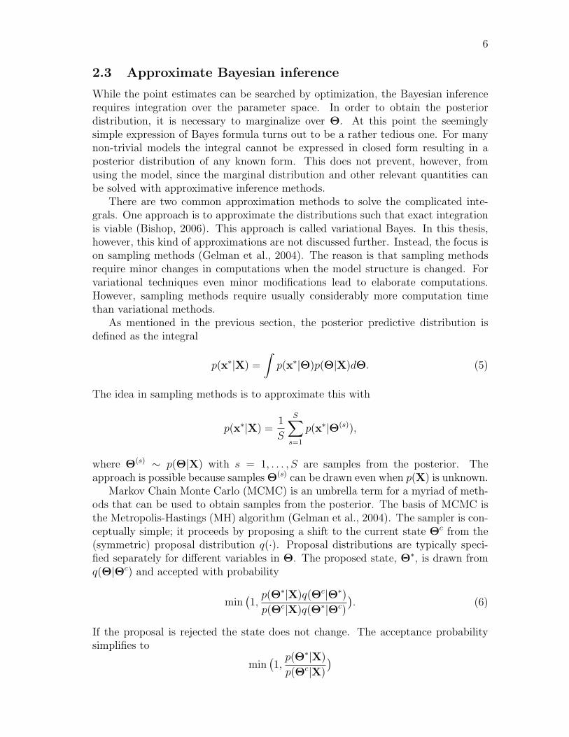
The training error is denoted as Jtrain and the error for future data as Jtest.Demonstration of the model selection procedure is given in Figure 1. The modelcomplexity (usually measured by the number of the parameters in the model) needsto be set suitably. Too complex model overfits, that is, it describes well trainingdata but does not generalize well. On the other hand, the model has underfitted ifboth errors are large.

In principle, model complexity could be chosen based on Jtest but this quantityis not known. By using a validation set we can approximate Jtest and determinemodel complexity (Bishop, 2006). The available data are split in two sets and oneis used for training and the other for validation. When the model begins to describeaspects of training data alone the prediction error increases or remains the same.For MAP estimation the validation set can be used to set the parameters of theprior as well.

8

Figure 1: Demonstration of model selection. Low complexity models underfit andboth training and testing errors are large. On the other hand, too complex modelsoverfit and the test error is large. Suitable compromise of model complexity resultsin best performance.

2.5 Why Bayesian modeling?

The difference between maximum likelihood(ML) and Bayesian inference methodsis critical. For Bayesian inference the uncertainty is expressed in parameter valuesin the form of prior distribution and the corresponding posterior distribution issought. ML assumes that the observed data set has unique true parameters andthe uncertainty is assumed only for the observed data, i.e., the observed data setis one random realization of the true process. The solutions found by ML lie inthe space spanned by the observed data, making this approach well justified forlarge data sets. For the Bayesian method the space of parameters is constrainedby the prior distribution. For example, in extreme cases the parameter value Θ0

with zero prior probability, p(Θ0) = 0, results in posterior with zero probability,p(X|Θ0)p(Θ0) = 0.

Predictive quality of ML for machine learning methods depends on the numberof training samples. Simple illustration of this effect is demonstrated by classicalcoin tossing example. If a coin has been tossed two times and both tosses landedheads, ML deducts that all future tosses are also heads. ML is overly confident inits predictions. In Bayesian inference a prior favoring a fair coin is used, and theposterior distribution after the two tosses contains the prior knowledge resulting inrational inference for the future outcomes.

Briefly put, ML overfits to small data sets while computationally heavy Bayesianmethods flourish. However, this does not mean that Bayesian inference would belimited to only small data sets. For example, Salakhutdinov and Mnih (2008 (b)).apply Bayesian matrix factorization to a very large matrix.

9

3 Exponential family projection models

In the previous section the basic concepts of Bayesian modeling were discussed. Inthis section concrete models are introduced: Principal component analysis (PCA)and its extension to the exponential family. The section starts with explanationof the exponential family and then the PCA and its extensions are explained. Inthe end of this section, a brief review on related methods is given. The focus inthis section is on ML inference, whereas Bayesian inference solutions for this kindof models are presented in Section 6.2.

3.1 Exponential family distribution

Exponential family is a collection of distributions that can be used to approximateall relevant and common distributions usually encountered in machine learning andmodeling in general (Bernardo and Smith, 2000; Bishop, 2006; Gelman et al., 2004).

A univariate random variable x ∈ X ⊆ R (where X is a suitable subset of thereal-space, such as Z or R+) in the exponential family follows the distribution

p(x|θ) = exp(s(x)θ + lnh(x)− g(θ)), (7)

where θ ∈ K ⊆ R represents the natural parameters of the distribution, g(·) is thelog cumulant function that normalizes p(x|θ) to be a valid distribution, s(·) are thesufficient statistics, and h(·) is a function of the data alone.

To be more specific, (7) can be written as

p(x|θ) =h(x) exp(s(x)θ)∫

x∈X h(x) exp(s(x)θ)dx,

where

g(θ) = ln

∫x∈X

h(x) exp(s(x)θ)dx

is the normalization term. In this thesis distributions are confined to the naturalexponential family by assuming s(x) = x. An additional assumption is that theexponential family is regular, that is, the function h(·) does not depend on θ. Oth-erwise the family is said to be non-regular. Different choices of g(·) lead to differentexponential family distributions including Gaussian with known variance, Bernoulli,Poisson, and exponential. The functional form of g(·) depends on the data domainX and h(·).

The function g(θ) has interesting properties. By differentiating it with respect

10

to the parameters one obtains

d

dθg(θ) = g′(θ)

=d

dθln

∫x∈X

h(x) exp(xθ)dx

=

∫x∈X xh(x) exp(xθ)dx∫x∈X h(x) exp(xθ)dx

=

∫x∈X

xh(x) exp(xθ − g(θ))dx

= Ep(x|θ)[x] = µ.

That is, the derivative of g(θ) defines the expectation of x. Similarly the nth ordercumulants can be calculated by differentiating g(θ) n times.

Exponential family distributions can also be expressed in an alternative parametriza-tion. Above the natural parametrization was presented, while the mean valueparametrization, p(x|µ), is more commonly known. Some examples of the exponen-tial family distributions are collected in Table 1 presenting details of the differentparametrizations and of the domains of the data and the parameter. For example,it can be seen that for the Gaussian data the two different parameterizations areequivalent.

As a concrete example, for X = {0, 1} and h(x) = 1 the log cumulant functioncan be written by replacing integration by summation as

g(θ) = ln(1 + exp(θ)).

These assumptions lead to the Bernoulli distribution that belongs to the exponentialfamily. Using the identity exp(ln f(x)) = f(x) and writing the logarithm of Bernoullidensity function one obtains

ln p(x|µ) = x lnµ+ (1− x) ln(1− µ) = x lnµ

1− µ+ ln(1− µ) (8)

and parameterizes

θ = lnµ

1− µ(9)

to obtain inverse mapping

µ =1

1 + exp(−θ). (10)

Finally inserting (9) and (10) to (8) gives (7) with lnh(x) = 0.

3.1.1 Conjugate priors

Exponential families have many interesting properties. One property is that for ev-ery member of exponential family there exists a so-called conjugate prior distributionfor θ:

p(θ) ∝ exp(λθ − νg(θ)

). (11)

11

Table 1: Examples of distributions in the exponential family. Symbol dom() isused to denote the domain of the argument. The derivative of g(·) is the so calledlink function that is needed to transform natural parameter to the data space. InSection 3.3.1 it is shown how the link function arises naturally in exponential familyprojections.

Gaussian, σ2 = 1 Bernoulli Poisson Exponential

p(x|µ) exp(−1/2(x−µ)2)√2π

µx(1− µ)1−x exp(−µ)µx

x!µ exp(−µx)

dom(x) R {0, 1} {0, 1, 2, . . . } R+

dom(µ) R [0, 1] R++ R++

θ µ ln µ1−µ lnµ −µ

dom(θ) R R R R−−g(θ) 1

2θ2 ln(1 + exp(θ)) exp(θ) − ln(−θ)

g′(θ) θ (1 + exp(−θ))−1 exp(θ) −θ−1

lnh(x) −12(x2 + ln 2π) 0 − lnx! 0

A prior is defined to be conjugate if the corresponding posterior distribution is ofthe same form as the prior. The posterior distribution can be written

p(θ|x) ∝ p(x|θ)p(θ) = exp((x+ λ)θ − (1 + ν)g(θ)

)and it is indeed of the same form as (11). The main motivation for using such priorsis that the posterior distributions can be derived analytically. The prior parameterscontrol the strength of the prior. Values near 0 for λ and ν correspond to weaklyinformative prior, resulting to p(θ|x) ∝ p(x|θ). The corresponding conjugate priorsfor some of the distributions in Table 1 are presented in Table 2.

Table 2: The conjugate priors with alternative parametrization. For example,Bernoulli-beta denotes that the beta distribution is the conjugate prior for theBernoulli distribution. The normalization term Z(·), as g(·) in (7), depends onthe values of the parameters of the distribution.

Gaussian-Gaussian Bernoulli-beta Poisson-gammap(µ) 1

Z(µ0,σ2)exp(− 1

2σ2 (µ− µ0)2) 1

Z(α,β)µα(1− µ)β 1

Z(α,β)µα−1 exp(−µ/β)

µ0 ∈ R, σ2 > 0 α, β > 0, 0 < µ < 1 α, β > 0, µ ≥ 0λ µ0/σ

2 α α− 1ν 1/(2σ2) β + α 1/β

12

3.2 Principal component analysis

As described briefly in Section 1, PCA is a frequently used dimensionality reduc-tion method (See Jolliffe, 1986). The purpose of PCA is to find a low-dimensionalrepresentation of data that can be used, for example, for data compression or visu-alization.

There are two common ways to derive PCA. The first is possibly more common,while the latter provides a deeper understanding of the method. In the first waythe PCA can be seen as a method that seeks for projections that capture maximalvariance in the projected space (Hotelling, 1933). The other way is to search for low-rank structure of the data by minimizing the reconstruction error between the low-rank approximation and the original data (Pearson, 1901). Below both approachesare presented, omitting unnecessary details that can be found from any reasonabletextbook account on machine learning, such as (Bishop, 2006).

For the remainder of this thesis it is assumed that N observed realizations ofD-dimensional random variable x ∈ RD are collected in the matrix

X =(

x1 x2 . . . xN)T ∈ RN×D.

PCA seeks components, vi ∈ RD, i = 1, . . . , K that capture maximal variance of theprojected data vTx under the constraint that different components are orthogonal,that is, vTi vj = Iij, where I is a K × K identity matrix. The components aredemonstrated in Figure 2 for simulated data. The components correspond to thefirst K leading eigenvectors of the sample covariance matrix

C =1

N

N∑n=1

(xn − µ)(xn − µ)T ,

where µ = 1N

∑Nn=1 xn is the sample data mean. The eigenvectors of C, denoted

by the columns of W ∈ RD×D, correspond to the solutions of the linear system,CW = WΛ, where Λ is a diagonal matrix with eigenvalues λi, i = 1, . . . , D, on itsdiagonal sorted as λ1 ≥ λ2 ≥ · · · ≥ λD, and W is an orthonormal matrix satisfyingWTW = WWT = I.

Choosing the K first eigenvectors of W in the columns of V ∈ RD×K the pro-jection of data to the so-called latent variables is defined as

un = VT (xn − µ).

Collecting latent variables in matrix U =(

u1 u2 . . . uN)T

and by denoting

xn = xn − µ the projection can be written as U = XV. For K = D, VVT = I andX = UVT . For K < D the equality does not hold, assuming that the rank of Xis D, but the approximation X ≈ UVT is still optimal in some sense. SpecificallyPearson (1901) proves, that the PCA solution is the one that minimizes the costfunction J written as

J =N∑n=1

||xn − xn||2 =N∑n=1

||xn −Vun − µ||2, (12)

13

Figure 2: Illustration of PCA. The two PCA projections are plotted for the simulated2-dimensional data. The first projection captures maximal variance while the secondis constrained to be orthogonal to the first. The lengths of the arrows are scaledaccording to the captured variance.

where the approximation x of the original data x is constrained to be low-rank.In order to proceed towards probabilistic modeling, it is next shown how the cost

function J of (12) stems from assuming a probabilistic model for x.

3.2.1 Maximum likelihood principal component analysis

If the matrix elements are assumed to be conditionally independent and exchange-able given the parameters , the probabilistic model for the data can be writtenas

p(x1, . . . .xN |θ1, . . . ,θN) = p(X|Θ) =N∏n=1

p(xn|θn) =N∏n=1

D∏d=1

p(xnd|θnd). (13)

The assumption of conditional independence can be justified if Θ is flexible enoughto capture the dependencies in x. The PCA model is obtained by constraining Θ =(θ1 θ2 . . . θN

)T, where θn = Vun +µ, and assuming that p(x|θ) corresponds

to the Gaussian distribution with known variance.Following ML inference, the complete data log-likelihood is written as

L = ln p(X|Θ) =N∑n=1

ln p(xn|θn) =N∑n=1

D∑d=1

ln p(xnd|θnd)

=N∑n=1

D∑d=1

− ln√

2πσ2 − 1

2σ2(xnd − θnd)2

= −ND ln√

2πσ2 − 1

2σ2

N∑n=1

||xn −Vun − µ||2.

It can be shown that the log-likelihood corresponds to the cost function of the PCAmodel, L = −J , omitting terms that do not depend on the parameters and assumingσ2 = 1/2.

14

3.3 Exponential family principal component analysis

The immediate extension of PCA to the exponential family is given by noting thatthe Gaussian distribution belongs to the exponential family. The generalization ofPCA to the exponential family (EPCA) retains from PCA the property that theparameters of the distribution are represented as θ = Vu + µ, while the likelihoodfunction p(xnd|θnd) changes according to different assumptions on the noise model(Section 3.1). EPCA provides a unified framework for PCA for different data types.The only difference in the likelihood function between different distributions in ex-ponential family is the function g(·), because h(·) does not depend on parameters.

An important difference between different assumptions for p(x|θ) is in predic-tions. Wrong assumptions for p(x|θ) can lead to predictions out of the domain ofdata. For example, in missing value imputation task for binary data the Gaussianassumption leads to predictions in R, while all the values should be exactly 0 or 1.If data is known to be binary it is recommended to make the assumption that thelikelihood corresponds to the Bernoulli distribution, because then the only kind ofnoise possible is bit flips, i.e., 1 changes to 0 or vice versa.

3.3.1 Maximum likelihood inference for exponential family principalcomponent analysis

To find the maximum likelihood estimates for U and V for an observed data matrixX, the data log likelihood needs to be maximized. To simplify the notation denoteU :=

(U 1

)and V :=

(V µ

), incorporating the mean parameter in UVT .

Maximization of the log likelihood, written in vector-matrix form,

L = Tr[X(UVT )T ]−∑nd

g(UVT ) (14)

can be performed by finding a point satisfying ∇L = 0. Above Tr[C] =∑

i Cii isused to denote the trace of the square matrix C. The notation for g(C) (also forg′(C)) is overloaded, for a matrix argument it corresponds to element-wise applica-tion. Local optima of (14) are defined as points that satisfy the condition, ∇Ll = 0.However, there may exist a better solution corresponding to the global maximumL∗ with the property L∗ ≥ Ll ∀l.

The gradient of (14) with respect to the latent variables can be written as

∇UL =(X− g′(UVT )

)V,

and with respect to the projection matrix as

∇VL = UT(X− g′(UVT )

).

Maximum likelihood inference for EPCA thus results in matrix factorization writtenas X ≈ g′(UVT ). For suitably large K the approximation becomes the equivalenceX = g′(UVT ). The derivative of the log cumulant function g(·) hence provides alink between the data and the natural parameter space. For classical PCA with

15

Gaussian likelihood the parameter space and the data space are equivalent (Section3.1) and hence X ≈ UV. That is, the parameters and data have linear relationshipand inference can be carried out by solving linear systems (Section 3.2). In thegeneral case the relationship between the parameters and the data is not linear anditerative optimization methods need to be applied (discussed in Section 6.1).

3.4 Probabilistic principal component analysis

Despite the use of p(x|θ) to define the PCA cost function, it does not provide fullprobabilistic model as the variance term was assumed known. Next it is shown howPCA can be interpreted as a a full probabilistic model. Even though the presenteddetails apply only for the Gaussian model, EPCA has essentially the same properties.This section gives more detailed view of the PCA model, essentially, answeringquestions like what kind of dependencies PCA can capture and to what kind of datait is suitable to apply for.

In Section 3.1 only univariate exponential family distributions were presentedin detail. Details for the multivariate distributions such as multinomial, Gaussianwith unknown variance parameter, and multivariate Gaussian, that do belong tothe exponential family, were omitted but can be found from (Bernardo and Smith,2000). For now on N (µ,Σ) is used to denote the multivariate Gaussian densitywith mean parameter µ and covariance matrix Σ.

The PCA model can be written as

x = Vu + µ+ ε, (15)

where ε ∼ N(0, σ2I) is a noise term, and the subscripts used for different data pointsare removed for clarity. Essentially, θ = Vu+µ is assumed to be a noiseless versionof the observed noisy data point x.

By assuming that the latent points follow the prior distribution p(u) = N (0, I),one can write the mean of x under the model assumptions with known V and µ as

E[x] = E[Vu + µ+ ε] = µ, (16)

because E[u] = E[ε] = 0, and because expectation is a linear operator. The covari-ance of x can be written as

E[(x− E[x])(x− E[x])T ] = E[(x− µ)(x− µ)T ] (17)

= E[(Vu + ε)(Vu + ε)T ] (18)

= E[VuuTVT + VuεT + εuTVT + εεT ] (19)

= VVT + σ2I, (20)

because the noise and the latent variables are assumed to be independent, E[uεT ] =E[εuT ] = 0, E[uuT ] = I, and E[εεT ] = σ2I. It can be seen how V capturesthe covariances of x. By the assumption of Gaussian noise and latent variables itcan be shown (Bishop, 2006) that the marginal likelihood, or equivalently the datadistribution, is another Gaussian distribution written as

x|V,µ, σ2 ∼ N (µ,VVT + σ2I). (21)

16

This is directly obtained by solving

p(x|V,µ, σ2) =

∫p(x|u,V,µ, σ2)p(u)du. (22)

Tipping and Bishop (1999) show that maximizing the marginal likelihood withrespect to the parameters, µ, V and σ2, leads to the PCA solution. The maximumlikelihood estimates are

µ =1

N

N∑n=1

xn (23)

V = WK(ΛK − σ2I)1/2R (24)

σ2 =1

D −K

D∑n=K+1

λn, (25)

where WK corresponds to K leading eigenvectors of C and R is an arbitrary K×Korthogonal matrix. The parametrization of the projection matrix is defined up to arotation of the PCA solution, as can be seen by writing

VVT = VRRTVT = VVT ,

since RRT = I. However, the actual PCA projections can be solved up to a signchange by replacing the sample covariance matrix with VVT + σ2I for the PCAalgorithm in Section 3.2.

The model is named probabilistic PCA (PPCA) and it is called generative be-cause new data can be generated from it. This is important property, and illustra-tions of it are given in Section 3.1.

Tipping and Bishop (1999) further show that the predictive distribution is yetanother Gaussian distribution,

p(u∗|x∗) = N(u∗|M−1VT (x∗ − µ), σ2M),

where M = VTV + σ2I. The mean of the distribution is equivalent to the PCAsubspace, up to rotation R.

Comparing PPCA to PCA, the most significant difference is the global noiseterm, σ2. Further, it was shown above that traditional PCA makes tacit assumptionof Gaussian data and latent variables.

3.5 Demonstrations

For the PPCA model exact marginalization of the latent variables can be done, lead-ing to the multivariate Gaussian distribution (21). However, for the other membersof the exponential family this marginalization cannot be performed in closed form.

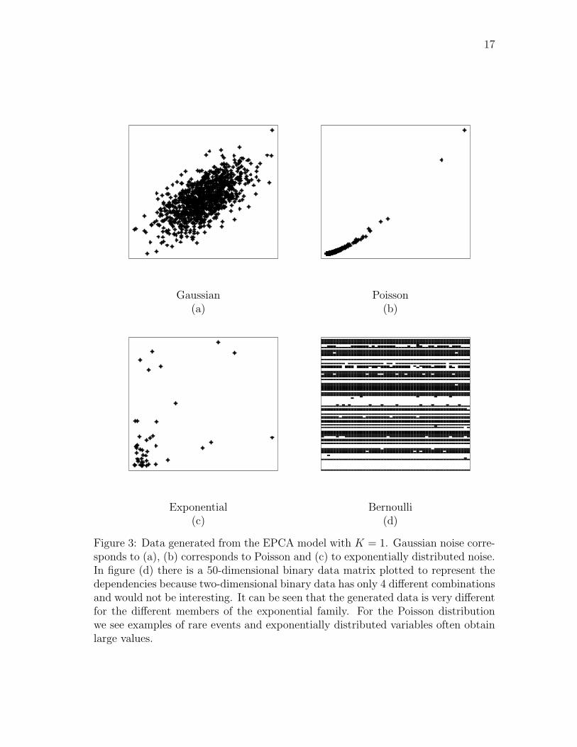
For demonstration, different data sets are drawn from the EPCA model forvarious data types, and visualized in Figure 3 retaining the assumption that u ∼N (0, I). From Figure 3 it can be seen how the distributional assumptions completelychange the shape of the data.

17

Gaussian Poisson(a) (b)

Exponential Bernoulli(c) (d)

Figure 3: Data generated from the EPCA model with K = 1. Gaussian noise corre-sponds to (a), (b) corresponds to Poisson and (c) to exponentially distributed noise.In figure (d) there is a 50-dimensional binary data matrix plotted to represent thedependencies because two-dimensional binary data has only 4 different combinationsand would not be interesting. It can be seen that the generated data is very differentfor the different members of the exponential family. For the Poisson distributionwe see examples of rare events and exponentially distributed variables often obtainlarge values.

18

3.6 Related methods

The likelihood p(x|θ), where θ is low-rank, is used in many other famous machinelearning methods for matrix factorization. The methods differ in multiple ways: inthe form of the likelihood function as shown above, the factorization of θ, or theconstraints and prior distributions set for the low-rank decompositions.

In this thesis, linear factorization of θ is considered. However, non-linearitiescan be taken into account as well. The problem is then how to define these non-linearities. Lawrence (2005) considers extension of PCA to Gaussian processes.Instead of marginalizing the latent variables, marginalization of V is performedassuming a column-wise Gaussian prior. Further, the kernel trick is used to makethe model non-linear. Another non-linear Bayesian approach is given by Lian (2009);non-linear dimensionality reduction is achieved by applying in the latent space localprojections that are smoothed with a Markov Random Field-type prior.

For EPCA the relationship between the parameters and the data is expressedwith a non-linear function. Using suitable non-linearities while still assuming Gaus-sian data can be seen as heuristic approach for taking correct noise type into account(see for example (Salakhutdinov and Mnih, 2008; Ma et al., 2008)). Suitable non-linearities are readily proposed by g′(·). Mathematically this can be written as thefollowing observation equation

x = f(Vu) + ε,

where ε ∼ N(0, σ2I) and f(·) is a non-linear function. Incorporation of non-linearities to the squared loss function complicates inference by introducing localminima (Gordon, 2002).

By changing the prior distribution of the latent variables to Dirichlet or multi-nomial the task of dimensionality reduction is turned into clustering, for example(Heller et al., 2008). Bingham et al. (2009) compare two different priors for thelatent variables, continuous and constrained, concluding that by constraining thelatent variables they become competitive and in the other case they work in col-laboration. This affects the interpretation of components. In non-negative matrixfactorization the components of θ are constrained to be positive (Lee and Seung,2001).

In general, determining the noise distribution can be challenging. Guo and Schu-urmans (2008) proposed a more flexible framework where the function g(·) is solvedby the sample-based approximation

g(θ) ≈ ln

(1

N

N∑i=1

exp(xiθ)

).

The observed data hence determines the distribution in question. Guo (2009) alsoincorporates this approximation. Another approach would be to use some modelselection procedure to choose the most likely distribution for the data.

19

4 Models for paired data

The methods considered so far are suitable for the analysis of a single data matrix.One of the main contributions of this thesis is to present how multi-source learningmethods arise as special cases of the EPCA model.

Two random variables, y1 ∈ KD1 and y2 ∈ KD2 , are paired if the samples in thetwo co-occur. Co-occurring samples are generated in pairs of items, y1 and y2. Byconcatenating the two sources as xT =

(yT1 yT2

)several projection methods for

paired data sources can be written as EPCA of x, that is, as factorizations of theform θ = Vu.

Different kinds of models are obtained by specifying different constraints on V.Many of the decisions in practical modeling, such as the choice of prior distributionsand inference algorithm, are independent of such restrictions imposed on V, andhence the unified framework helps in developing practical algorithms for variouspaired data analysis tools.

Below only the likelihood functions for the proposed models are presented, whilethe corresponding prior distributions are presented in Section 5, as these are sharedbetween all the methods.

4.1 Supervised exponential family principal component anal-ysis

Supervised PCA (SPCA) is the simplest model for paired data. One of the sources,say y1, is treated as a target variable, and the task is to find a low-dimensionalrepresentation of y2 that helps in predicting the target.

The task is termed as supervised dimensionality reduction. Instead of findinga latent variable description of y2, the lower dimensional manifold is obtained forprediction of y1. EPCA as preprocessing for y2 alone would not take the targetinformation into account, and hence would not necessarily produce latent variablespredictive of y1.

The original SPCA formulation (Yu et al., 2006) as well as the supervised EPCA(Guo, 2009; SEPCA) follow this idea, the crucial difference being that the lattermakes the correct distribution assumption for the target variables. If y1 with D1 = 1is continuous the task is called regression and if binary the task is classification. Forthe regression a typical assumption for y1 is a Gaussian distribution while for binaryclassification Bernoulli distribution is a more justified choice. For D1 > 1 multi-regression or multi-classification tasks arise that can be defined as special cases ofmulti-task learning (Caruana, 1997): multiple prediction tasks share the same input,the latent variables.

Due to the assumption of conditional independence between y1 and y2, giventhe parameters, the SEPCA likelihood can be written as

p(x|u,V,µ) =p(y1|u,V1,µ1)p(y2|u,V2,µ2)

or, more clearly, to clarify the dependence between data and parameters, as

p(x|θ) = p(y1|θ1)p(y2|θ2).

20

where θ =

(θ1

θ2

)= Vu + µ,

µ =

(µ1

µ2

)and

V =

(V1

V2

)so that the columns are split according to the features in x.

Briefly put, SEPCA is EPCA of x. The features are treated equally and hencethis approach provides weak supervision as the model aims to capture all depen-dencies between the elements of x. The predictive performance of such a modelimproves if one does not attempt to model y2 perfectly; after all, the ultimate taskis to predict y1 and the covariates should be modeled only to the degree they help inthat task. Rish et al. (2008) proposed an approach to weight the generative parts,resulting in the model likelihood

p(x|θ) = p(y1|θ1)p(y2|θ2)α, (26)

where α controls the relative importance of modeling the two sources. When smallvalues are chosen for α less modeling power is spent on the covariates, resulting inincreased predictive performance.

Instead of treating α as an arbitrary control parameter, it can be interpreted asa fixed variance parameter in the general exponential family formulation (Gelmanet al., 2004). Dropping the assumption of identical variance for all features, (7) canbe written as

p(x|θ) =D∏d=1

exp

(wi(xiθi + lnh(xi)− g(θi)

)),

where w is a vector consisting of ones for y1 and α’s for y2,

wT =(

1 . . . 1 α . . . α).

The interpretation has close relationship to maximum likelihood factor analysis (FA)(Bishop, 2006). In FA the noise follows ε ∼ N (0,Σ), where Σ is diagonal matrixwith separate elements on its diagonal, while PCA assumes that all elements areequal. For Gaussian data the w parameter can be recognized as an inverse varianceparameter. However, even this formulation does not provide easy ways of infer-ring α from data, since changing it would affect the normalization constant of thedistribution p(x|θ).

4.1.1 Applications of supervised exponential family principal compo-nent analysis

In general SEPCA can be used in data integration, combining multiple sources ofinformation to improve prediction accuracy. Williamson and Ghahramani (2008)and Ma et al. (2008) considered joint models for data combination in recommender

21

systems assuming Gaussian data, while Singh and Gordon (2008) present moregeneral framework performing modeling in the exponential family.

Recommender systems aim to suggest for users movies they would like to seebased on the movie ratings of other users. This is a missing value imputation prob-lem. Incorporating auxiliary data of users and/or movies may improve predictionaccuracy. Ma et al. (2008) considered fusion of social network data of users toimprove movie recommendation accuracy. Motivation is that friends usually havesimilar taste and they recommend movies to each others.

SEPCA can also be seen as incorporating ’background knowledge’ to EPCAmatrix factorization. Typically the latent variables are assumed some simple priordistribution p(u). Recent approach of Bo and Schmisesku (2009) introduce so-calledsupervised latent variables, that is, the latent variables depend on y2. Mathemat-ically the assumption can be written as p(u|y2). However, the two approaches areequivalent. This can be seen by writing

p(y1|u)p(y2|u)p(u) = p(y1|u)p(u|y2)p(y2)

p(u)p(u) = p(y1|u)p(u|y2)p(y2).

4.2 Exponential family partial least squares

An alternative way of improving the predictive performance in supervised learningtasks is to allow the covariates to have structured noise that is independent of thetarget variable. This leads naturally to a classical linear supervised dimensional-ity reduction method of partial least squares (PLS) and its probabilistic variants(Gustafsson, 2001; Nounou et al., 2002). These models are restricted to Gaussiandata. In this thesis, the correct data type is taken into account, introducing theexponential family partial least squares (EPLS).

The key idea in PLS is that not all variation in y2 is relevant for predicting y1.A novel way incorporating that knowledge is proposed in the model by restrictingsome of the components to only model y2. By factoring uT =

(uTS uT2

)and V as

V =

(VS1 0VS2 V2

),

where S indicates variables shared between the data sources, the model can still bewritten as θ = Vu + µ. The model complexity is governed by fixing the ranks ofthe various parts. Denoting the rank of uS by KS and the rank of u2 by K2, thezeros in V make sure the last K2 columns of u will have no effect on y1. In moreintuitive terms, the parameters can equivalently be written as

θ1 = VS1uS + µ1

θ2 = VS2uS + V2u2,+µ2. (27)

which makes explicit the assumption that all variation in the target variable mustcome from the shared latent sources, while the covariates are created as an additivesum of the shared and source-specific variation.

22

(a) (b)

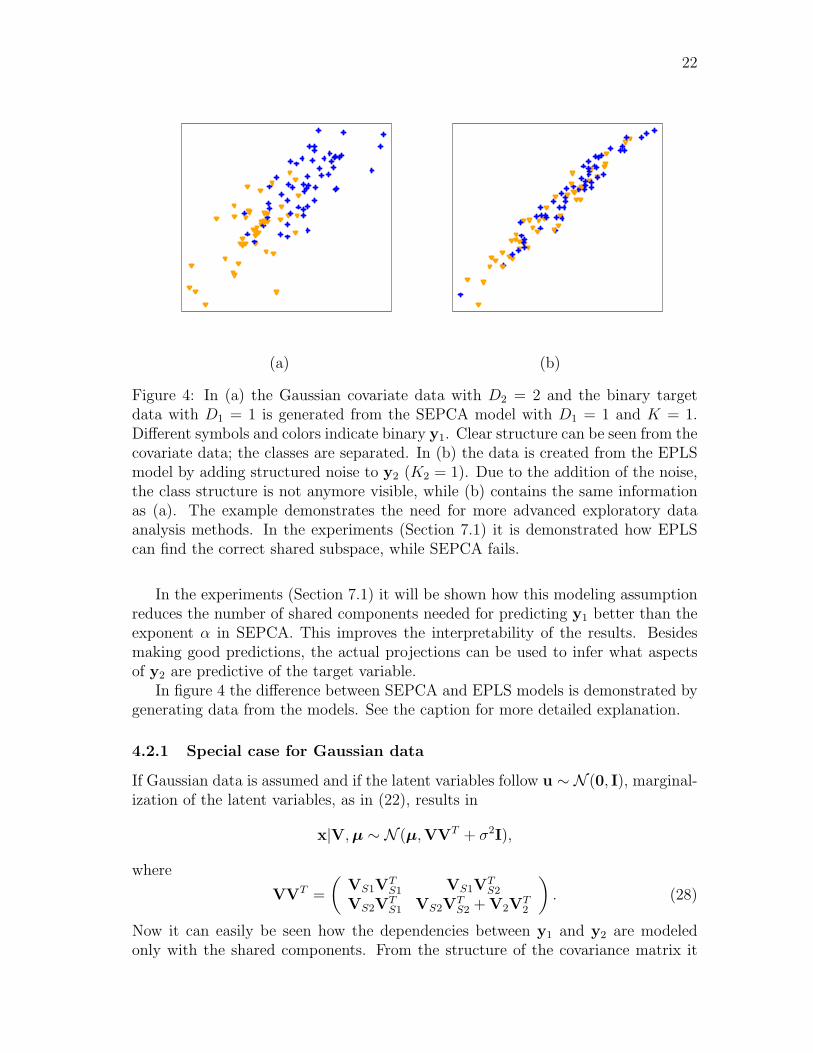
Figure 4: In (a) the Gaussian covariate data with D2 = 2 and the binary targetdata with D1 = 1 is generated from the SEPCA model with D1 = 1 and K = 1.Different symbols and colors indicate binary y1. Clear structure can be seen from thecovariate data; the classes are separated. In (b) the data is created from the EPLSmodel by adding structured noise to y2 (K2 = 1). Due to the addition of the noise,the class structure is not anymore visible, while (b) contains the same informationas (a). The example demonstrates the need for more advanced exploratory dataanalysis methods. In the experiments (Section 7.1) it is demonstrated how EPLScan find the correct shared subspace, while SEPCA fails.

In the experiments (Section 7.1) it will be shown how this modeling assumptionreduces the number of shared components needed for predicting y1 better than theexponent α in SEPCA. This improves the interpretability of the results. Besidesmaking good predictions, the actual projections can be used to infer what aspectsof y2 are predictive of the target variable.

In figure 4 the difference between SEPCA and EPLS models is demonstrated bygenerating data from the models. See the caption for more detailed explanation.

4.2.1 Special case for Gaussian data

If Gaussian data is assumed and if the latent variables follow u ∼ N (0, I), marginal-ization of the latent variables, as in (22), results in

x|V,µ ∼ N (µ,VVT + σ2I),

where

VVT =

(VS1V

TS1 VS1V

TS2

VS2VTS1 VS2V

TS2 + V2V

T2

). (28)

Now it can easily be seen how the dependencies between y1 and y2 are modeledonly with the shared components. From the structure of the covariance matrix it

23

can be deduced that K2 should be set high enough in order to prevent the sharedcomponents to capture covariate-specific variation. The structure of covariance ma-trix for the PCA model is identical to (28), except for omitting V2V

T2 . This means

that PCA captures all dependencies, ignoring whether they are shared or not.For distributions other than Gaussian, marginalization of the latent variables

can no longer be performed in closed form, but the presented model propertiesremain: the dependencies between y1 and y2 are still captured in VS1 and VS2.The covariate-specific variables can be seen as nuisance parameters that usually arenot of interest but necessary to extract the correct components.

4.3 Exponential family data fusion

Going beyond mere prediction problems, a common task in analysis of paired datais finding what is shared between the two data sources. This is a kind of data fusiontask: compress two data sources into a representation that captures the common-alities between the two. Alternatively, one can further represent the source-specificvariation present in each of the sources separately, independent of the other source.The problem is traditionally solved by canonical correlation analysis (Hotelling,1936), or its kernelized variant (Bach and Jordan, 2002), that have been appliedto a range of practical problems such as extracting shared semantics of documenttranslations (Vinokourov et al., 2003) and discovering dependencies between imagesand associated text to be used as preprocessing for classification (Farquhar et al.,2006).

PCA seeks projections that capture maximal variance in the projected space,whereas CCA can be seen as a method seeking for two projections maximizingcorrelation between the projected data. Similarly to PPCA presented in Section 2,it can be shown that probabilistic CCA assumes Gaussian latent variables and isequivalent to assuming a certain Gaussian model for the data (Bach and Jordan,2005). In this thesis this assumption is removed presenting a novel generalizationof CCA to the exponential family, termed ECCA for brevity. This is necessary, forexample, for text analysis with the generative approach, since text documents arenaturally described as binary collections of word occurrences or as count data.

First the CCA model and the corresponding probabilistic interpretation are ex-plained. Secondly ECCA is presented. Finally the combination of EPLS and ECCAmodels is presented that result in supervised ECCA (SECCA). Both ECCA andSECCA are novel contributions of this thesis.

4.3.1 Canonical correlation analysis

CCA aims to find linear transformations for the two random variables, y1 and y2,with N realizations collected in matrices Y1 and Y2 such that the projected data,y1 = Y1w1 and y2 = Y2w2, is maximally correlated. We denote the sample covari-ance matrix of X =

(Y1 Y2

)as

C =1

N

(YT

1 Y1 YT1 Y2

YT2 Y1 YT

2 Y2

)=

(Σ11 Σ12

Σ21 Σ22

)

24

assuming that the data sets are centered. Correlation for the projected data can bewritten as

ρ =yT1 y2√

yT1 y1

√yT2 yT2

=wT

1 YT1 Y2w2√

wT1 YT

1 Y1w1

√wT

2 YT2 Y2w2

=NwT

1 Σ12w2√NwT

1 Σ11w1

√NwT

2 Σ22w2

=wT

1 Σ12w2√wT

1 Σ11w1

√wT

2 Σ22w2

. (29)

Maximization of (29) can be done by constraining wT1 Σ11w

T1 = wT

2 Σ22wT2 = 1 and

applying the technique of constrained optimization. Multiple projections w1i andw2i with i ≤ min(D1, D2) are constrained to be uncorrelated, wT

1iΣ11wT1j = Iij, and

similarly for w2i. The solution for K vectors, collected as columns in W1 and W2,corresponds to the K first leading eigenvectors of the generalized eigenvalue problem(

0 Σ12

Σ21 0

)(w1

w2

)= ρ

(Σ11 00 Σ22

)(w1

w2

).

Proof and details of the constrained optimization are omitted, but can be foundfrom (Shawe-Taylor and Cristianini, 2004).

4.3.2 Probabilistic canonical correlation analysis

CCA can be interpreted as a maximum likelihood solution of a certain probabilisticmodel. Latent variables are defined as uT =

(uTS uT1 uT2

)and

V =

(VS1 V1 0VS2 0 V2

)for the model

x|u,V,µ ∼ N (Vu + µ, σ2I) (30)

following the presentation of Archambeau and Bach (2009).Assuming that latent variables follow u ∼ N (0, I), marginalization of the latent

variables results inx|V,µ ∼ N (µ,VVT + σ2I), (31)

where

VVT =

(VS1V

TS1 + V1V

T1 VS1V

TS2

VS2VTS1 VS2V

TS2 + V2V

T2

).

For the above model Bach and Jordan (2005), denoting Ψ1 = V1VT1 + σ2I and

Ψ2 = V2VT2 +σ2I, show the connection to standard CCA. More precisely, maximum

likelihood estimate of (31) corresponds to the projections found by traditional CCA,up to rotation and scaling.

25

According to Theorem 2 by Bach and Jordan (2005), the maximum likelihoodestimates for the parameters of the model in (31) are

VS1 = Σ11W1M1

VS2 = Σ22W2M2

Ψ1 = Σ11 − VS1VS1

T

Ψ2 = Σ22 − VS2VS2

T

µ1 = µ1

µ2 = µ2,

where W1 and W2 are the CCA projection matrices, M1 and M2 are arbitrarymatrices such that M1M2 = P and the spectral norms are smaller than one andP is diagonal matrix with canonical correlations. The µ corresponds to the samplemean. It is further shown that the posterior expectations of the latent variables liein the space spanned by the CCA solution.

If M1 = M2 = M = P1/2R, where R is rotation matrix of size K, it can be seenthat the probabilistic solution does not in general correspond to the actual projec-tions of CCA. In standard CCA the projections are ordered by the correlation thusidentifying the projections up to a sign change. However, Archambeau et al. (2006)provide a method identifying the actual subspace of CCA also for the probabilisticsolution.

4.3.3 Exponential family canonical correlation analysis

Generalization of CCA to the exponential family is defined as model p(x|θ), where

θ1 = VS1uS + V1u1 + µ1

θ2 = VS2uS + V2u2 + µ2.

The notation is equivalent to Klami and Kaski (2008). The full model is illustratedin Figure 5, to clarify the role of the various parts of V.

4.3.4 Supervised exponential family canonical correlation analysis

Above it was described how ECCA can be used to extract mutual dependencies be-tween two data sets. Besides interpretation tasks, Tripathi et al. (2008) explore howthe shared subspace extracted by CCA can be used for classification. They proposeto use CCA as a preprocessing method. The method they consider can be seenas supervised CCA where the target information depends only on the shared latentvariables. By combining EPLS and ECCA, model for supervised shared componentscan be built. The novel algorithm is termed supervised ECCA (SECCA).

In the general case for M data sets, where y1 as in SEPCA (Section 4.1) is usedto denote targets, the data vector can be written as

xT =(

yT1 yT2 . . . yTM).

26

Figure 5: Graphical model for ECCA. Shared variables uS, VS1 and VS2 captureonly mutual dependencies between y1 and y2 while set-specific variation for y1 ismodeled with specific variables u1 and V1, similarly for y2. K denotes the ranks ofvarious parts and N refers to the number of observed samples.

The model structure is still written as θ = Vu + µ, where

uT =(

uTS uT2 . . . uTM).

and

V =

VS1 0 0 . . . 0VS2 V2 0 . . . 0VS3 0 V3 0

......

. . ....

VSM 0 0 . . . VM

In SECCA the target-specific variation is left out similarly as in EPLS in order tocapture shared predictive features of y1. To simplify modeling the covariance, thetrick of Rish et al. (2008) can be incorporated. That is, different values of w can beused to determine whether modeling power should be focused on prediction or not.By dropping y1 the model becomes ECCA for multiple views.

27

5 Priors for exponential family projections

Previously the likelihood functions for EPCA (Section 3) and its various extensions(Section 4) were presented. Following Bayesian inference prior distributions need tobe considered defining full joint probability model for the data and the parameters.Setting prior distributions for the parameters is a challenging part of Bayesian mod-eling and is an active research area. Typically, the choice of prior distribution is acompromise between complex and more realistic priors leading to complicated infer-ence, and simple priors chosen to guarantee efficient computation. Caution must betaken when placing priors to make sure that the resulting posterior is proper, thatis, the integral p(X) in (2) does not diverge to infinity.

Most of the research on EPCA-type models has focused solely on ML-solutionsor retained prior distributions from the Gaussian Bayesian models. In this thesis,instead, a general prior formulation that takes distribution-specific constraints forthe natural parameters into account is proposed.

5.1 Background

The first step of Bayesian modeling (see Section 2) is to write down the full prob-ability model for observed and unobserved variables, which in the case of EPCAresults in

p(u,V,µ,x|Θ) = p(x|u,V,µ)p(u,V,µ|Θ),

where Θ denotes the collection of all the hyperparameters, that is, the parametersof the priors.

The values for Θ need to set to some suitable values before conditioning ondata. However, setting these values is in general hard and one would like to setthese values automatically, i.e., learn the values for Θ from data. One possibilityis to treat Θ as random variables and place so-called hyperprior distribution for Θ.This kind of prior structure is also called hierarchical prior distribution (Gelmanet al., 2004). Bayesian inference results in averaging over multiple models that havedifferent Θ weighted by the hyperprior distribution, although, Θ can alternativelybe determined with cross-validation, as discussed in Section 2.4.

5.2 Joint prior

In this thesis a family of prior distributions is presented that incorporates certaincommon choices as special cases, while being an efficient way of altering the com-promise between conjugacy and flexibility in practical models.

Mohamed et al. (2009) extended the EPCA to a full Bayesian model, specifyingprior distributions directly for u and V. This approach is conceptually simple andstraightforward, but it is hard to determine which distributions to use. Mohamedet al. (2009) borrowed the assumption of normally distributed latent variables ufrom the Gaussian case, while taking V conjugate to the specific exponential family.The latent variables are assumed to be independent in the prior. Mathematically,

28

the prior is written as

p(U,V,µ|λ, ν,m,S, α0, β0) ∝ p(V|λ, ν)p(U|µ,Σ)p(µ|m,S)p(Σ|α0, β0), (32)

where, starting from right to left,

Σii ∼ iG(α0, β0), i = 1, . . . , K (Σ is a diagonal matrix) (33)

µ ∼ N (m,S) (34)

un ∼ N (µ,Σ), n = 1, . . . , N (35)

vk ∼ Conj(λ, ν), k = 1, . . . , K, (36)

where Conj denotes conjugate distribution and iG denotes the inverse-Gamma dis-tribution. The convenient property of (33) is that fixing the number of latent vari-ables, K, is not anymore that critical since unnecessary elements can be driven tozero, that is, Σkk ≈ 0 with suitable values for α0 and β0. Such a prior is generallytermed automatic relevance determination (ARD) prior and it is an example of ahierarchical prior (Bishop, 2006).

Unfortunately, (35) is a notoriously bad choice for some exponential family dis-tributions. For example, for the exponential distribution the domain of the naturalparameters is the set of strictly positive real numbers, which does not comply withnormally distributed u.

In this thesis an alternative novel solution is proposed by imposing the prior onthe product of the two variables, instead of formulating separate priors for each.For θn = Vun + µ it is easy to choose a prior conjugate to the specific exponentialfamily, which takes the correct distribution into account and makes the estimationof θ easy:

θn ∼ Conj(λ,ν), n = 1, . . . , N.

However, at the same time the connection to the actual factorization is lost;while the model is still parameterized through the low-rank matrices U and V, theU and V are unidentifiable. In practice, this kind of model can still be useful: Ifthe goal is not to analyze the actual components, but merely to find a low-rankapproximation of x (which is sufficient for example for reconstructing the originaldata from a compressed version), then it is feasible to place the prior directly on θ.

To combine the advantages of the two formulations, (i) separate priors and (ii)the prior for the product, the general prior is introduced

p(u,V|Θ, β) =1

Za(Vu)βb(u)1−βc(V)1−β, (37)

where β ∈ [0, 1]. For clarity, the prior for µ is dropped from the notation and itis taken to follow N(0, σ2

µI) with large σ2µ. The functions a(·), b(·), and c(·) can

be arbitrary non-negative functions over the domain of the parameters. The entirenormalization is done with Z, and hence the functions a(·), b(·) and c(·) need not benormalized. In practice, however, one would typically use standard distributions ofthe kind used in the above simpler prior assumptions. Then β = 0 and β = 1 reduce

29

the prior into the simpler alternatives, while other values of β produce combinationsof the two:

p(u,V|Θ, β = 0) ∝ b(u)c(V) (38)

p(u,V|Θ, β = 1) ∝ a(Vu). (39)

A useful property of the prior is that if a(·) is set so that it gives zero forvalues outside the domain of θ, then already a small β will be sufficient to restrictthe product of individually specified priors for u and V to be a legal distribution.This solves the problems of the prior distribution of Mohamed et al. (2009). Moregenerally, the compromise can be thought of as regularization, making the model lesssensitive for the specific choices of b(u) and c(V). That considerably simplifies thechoice of the distributions, and in practice simple component-wise Gaussian priors,

b(u) =K∏k=1

N(0, σ2U) (40)

c(V) =K∏k=1

D∏d=1

N(0, σ2V ), (41)

are used for both, which would not work in general without the regularizing a(Vu)term. The capabilities of the joint prior are demonstrated in Figure 6 for binarydata for which the conjugate distribution is the beta distribution. See the captionfor more details.

A practical challenge with this kind of a prior is that it is in general known only upto the normalization constant Z. This does not pose technical problems with MAP-or MCMC-based inference, since the normalization term cancels out. However, itmakes inference on possible hyper-parameters, such as σ2

U and σ2V above, of the prior

difficult. A sampling proposal for the hyper-parameters in the joint prior will needto evaluate the normalization term

Z(Θ) =

∫p(U,V|Θ, β)dΘ,

that, in general, cannot be computed analytically. In this thesis, a simple approachis used; the hyperparameters of a(Vu) are chosen for β = 1 and for b(u) and c(V) forβ = 0 using a validation set. In the experiments it is shown that already this simpleapproach leads to a better generalization ability than using either of the extremes.

30

β = 0 β = 0.33 β = 0.66 β = 1

Figure 6: Illustration of the joint prior. The two axes correspond to univariateu and v and the contours plot the probability of θ = uv under the joint prior,ln p(u, v) ∝ β

(λuv − g(uv)

)−(1− β

)(1/2u2 + 1/2v2

), where g(x) = ln(1 + exp(x))

with ln a(θ) = λθ− g(θ). That is, the prior correspond to the beta distribution thatis conjugate to the Bernoulli distribution. Additionally we set ln b(x) = ln c(x) =−x2/(2σ2) with σ2 = 1. The upper row corresponds to values λ = 10 and ν = 2λand the lower to values λ = 0 and ν = 10. In the lower row negative values for θare ruled out with suitably large value for β. With β = 1 the prior is improper.

31

6 Inference

After discussing both the likelihood functions and the prior distributions, the nextstep of Bayesian modeling is to derive the posterior distributions for all of the pa-rameters. Unfortunately, exact inference for the EPCA models is not possible. Twodifferent Markov Chain Monte Carlo (MCMC) sampling methods are discussed thatsuit different scenarios, but a brief detour on point estimation is first given; whilefull posterior inference is informative, it may be overkill in some applications.

6.1 Point estimates

Point estimates for the model parameters can be inferred from data by maximizingthe total log likelihood L as in (14). Gradient based optimization in the parameterspace is adopted to find stationary point of the likelihood, ∇L = 0, by updating theparameters in the direction of the gradient. MAP estimation is conceptually equallysimple; the priors only result in additive terms in L.

The optimization problem in the general case is large, because of the numberof variables, and difficult since it is not convex in both arguments. There havebeen many different proposals for finding point estimates. For Gaussian assumptionthe latent variables can be marginalized out, significantly decreasing the number ofparameters, and the resulting marginal likelihood is maximized (Roweis and Ghahra-mani, 1999; Tipping and Bishop, 1999).

Guo and Schuurmans (2008) proposed a convex optimization algorithm for themaximum-likelihood case of general exponential family PCA, while MAP estima-tion requires more generic optimization algorithms. While convex optimization al-gorithms converge to global optimum, they may be computationally demanding.Collins et al. (2002) present a simple alternating optimization, while Gordon (2002)applies sequential Newton updates. Rish et al. (2008), Schein et al. (2003) and Tip-ping (2001) use auxiliary functions that are limited to a subset of exponential familydistributions, typically Gaussian and Bernoulli distributions. The aim of the auxil-iary updates is to make an approximation of the cost function in the neighborhoodof the current point such that the gradient of this approximation can be presented inclosed form. In this thesis despite all the different optimization methods, conjugategradients are used following Srebro and Jaakkola (2003). In the experiments themethod has turned out to be sufficiently robust algorithm for sensible priors.

6.2 Advanced Markov Chain Monte Carlo methods

In Section 2.3 two MCMC algorithms, MH-algorithm and Gibbs sampler were dis-cussed. In this section two efficient samplers suitable for the general exponentialfamily projection models are presented. These are Hybrid Monte Carlo (HMC) andextended Gibbs sampler.

32

6.2.1 Hybrid Monte Carlo sampler

For full Bayesian analysis one can use Hybrid Monte Carlo (HMC) sampler, fol-lowing Mohamed et al. (2009). Compared to standard MCMC, the Hybrid MonteCarlo (HMC) typically converges faster in large state spaces due to utilizing the gra-dient information. The EPCA factorization typically has a very large state space,especially in the case of coupled data models where there are separate shared andsource-specific latent variables, making HMC a good choice here.

HMC has been applied for large systems such as neural networks (Neal, 1996) andGaussian processes (Barber and Williams, 1997), and is well described in many textbooks, see for example (MacKay, 2002). The idea behind HMC is to use moleculardynamic simulation for proposal distribution in the basic MH-algorithm.

HMC is an auxiliary variable sampler. Instead of drawing samples directly fromthe posterior distribution, the samples are drawn from an augmented distributionp(ψ, t) where t is an auxiliary variable and p(ψ) is used to denote the distributionfrom which one wishes to sample. To obtain marginal samples from the augmenteddistribution, the values for the auxiliary variables t are ignored. In HMC, t cor-responds to momemtum variables and the extended target density can be writtenas

p(ψ, t) = p(ψ)N(t|0, I).

HMC first draws the momentum variable t from a Gaussian distribution. ThenL ’frog steps’ are taken in ψ and t with step size τ . The values of ψ and t afterthe last step, L, are the proposal candidates for the Metropolis-Hastings acceptancestep. Pseudo-code for HMC is presented in Algorithm 1, where the frog steps arespecified.

The sampler has two parameters, L and τ . In the experiments L = 10 and τ isdrawn for each sample from the exponential distribution, following (Neal, 1993). Ifthe step size is too small the simulations are precise but the convergence towardsthe real posterior distribution can be slow. On the other hand, with large step sizemore proposals are rejected and hence the chain does not proceed optimally. As τ isdrawn from the exponential distribution τ is occasionally large, enabling large shiftsin the state space, yet most of the time the steps will be small.

6.2.2 Identification of components for interpretation

The sampler provides posterior samples for the parameters Θ, and one is typicallyinterested in obtaining marginal distributions of the whole joint posterior, for ex-ample for V. As presented in Section 2.3, marginalization can be performed bydiscarding all other variables that are not of interest. However, there remain severeunidentifiability problems with the proposed models; the marginal expectations ofposterior samples are useless. The natural parameters of the models can be repre-sented with {U,V,µ} in many different ways,

UVT = (URS)(S−1RTVT ) = UVT ,

where R is a unitary rotation matrix and S is a diagonal scaling matrix. Hence, Uor V cannot be averaged over the samples, making marginal posterior distributions

33

Algorithm 1 Hybrid Monte CarloL and µ0 are parameters of the algorithm. U[0,1] denotes the uniform distributionon interval [0, 1] and Exp(λ) the exponential distribution with parameter λ. Theoutput consists of samples ψ(s), s = 1, . . . , S.

1. Initialize ψ(0)

2. For s = 0 to S − 13. Sample a ∼ U[0,1], t

∗ ∼ N (0, I) and ε ∼ Exp(µ0)

4. Let ψ0 = ψ(s) and t0 = t∗ + ε∇p(ψ0)/25. For l = 1 to L take L frog steps

ψl = ψl−1 + εtl−1

tl = tl−1 + εl∇p(ψl)where εl = ε for l < L and εL = ε/2

6. If a < min

(1, p(ψL)

p(ψ(s))exp(−1

2

(tTLtL − t∗T t∗

))ψ(s+1) = ψL

t(s+1) = tLelse

ψ(s+1) = ψ(s)

t(s+1) = t∗

difficult to obtain. However, this commonly acknowledged identification problem,also noted by Mohamed et al. (2009) is solved in the following. It should also bekept in mind that even though the components of the product do not identify, theproduct UVT itself does, and UVT is already sufficient for predictions. Hence, thisunidentifiability issue is a problem only for interpretation of the components.

Denote Θ = UVT + 1µT as the matrix of natural parameters. Decompose Θwith PCA (Sect. 3.2). Mathematically the decomposition can also be written as

Θ = UΣVT ,

where Σ = diag(µ21 . . . µ

2D) and V =

(v1 . . . vD

)define the eigenvalues and

eigenvectors of ΘTΘvi = µ2i vi. Defining U = ΘVΣ−1 it can be further verified

that Θ = UΣVT = ΘVΣ−1ΣVT = Θ.One can average over the decomposed matrices made for S posterior samples

Θ(s) = U(s)Σ(s)V(s)T , where s = 1, . . . , S and use a simple method to correct forthe sign unidentifiability, i.e. UVT = (−U)(−VT ), of PCA. Collect the ith column

of U(s), denoted as U(s)i ∈ RN , in a matrix A =

(U

(1)i U

(2)i . . . U

(S)i

)T. For

the matrix A run K-means clustering algorithm (Bishop, 2006) setting K = 2. Thisis a very simple clustering task as the two cluster centers are c and −c. Finally,change the sign of samples in either cluster. The process is repeated for i = 1, . . . , D.Similar process is performed for the columns of V. Unfortunately, in the case of anyµi = µj for i 6= j the vectors vi and vj cannot be determined. See Figure 7 for anintuitive explanation.

34

Figure 7: The directions of two eigenvectors cannot be determined if the correspond-ing eigenvalues are equivalent. The differently dashed pairs of vectors correspondto the possible eigenvectors. The sphere illustrates a 2-dimensional subspace wherethe eigenvalues are equivalent. The direction of the first vector is random while thesecond has to be orthogonal to the first one.

An alternative, computationally less demanding method, is to average first overdifferent Θ(s) obtaining Θ = 1

S

∑Ss=1 Θ(s) and decompose the resulting single matrix.

This method is suitable for visualization applications since it suffices to plot theposterior means.

For Bayesian EPLS (BEPLS) and Bayesian ECCA (BECCA) one is usually onlyinterested in the shared components. Hence, only ΘS = USVS corresponding tothe shared components is decomposed.

In principle, it is also possible to add constraints, such as UTU = I, as in classicalPCA, in the sampler. Hoff (2007) showed that sampling with such constraints forU and V is possible, but points out that sampling can be painfully slow.

6.2.3 Extended Gibbs sampler

For the Gaussian Bayesian CCA (Klami and Kaski, 2007) analytic marginalizationof the source-specific variables is possible and the rotational ambiguity can be solvedrevealing the true canonical projections and the corresponding correlations (Section4.3). In ECCA, however, it is hard to make sure the modeling power is dividedcorrectly between the uS, u1, and u2. In principle the sampler explores the space ofsolutions correctly, but the convergence may be slow and the sampler may not mixwell.

In this thesis, a novel sampler that utilizes the more efficient solutions for theGaussian models as part of the sampler for the general exponential family is intro-duced. The practical sampling algorithm, coined GiBECCA, proceeds by alternatingtwo separate sampling steps. The algorithmic approach, explained next, is similarto how Hoff (2007) made inference for binary PCA. The intuitive idea is to alternatebetween two sampling stages. In one stage, the Θ is treated as data that a priorifollows normal distribution, and learn a factorization Θ = UVT for that. The otherstage then updates Θ, taking into account the exponential family likelihood and theactual data X.

After initialization (the first step of Algorithm 2), new values for the parameters

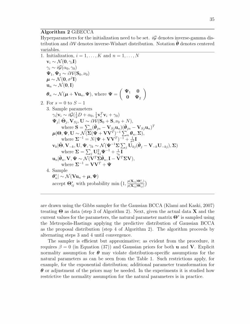
35

Algorithm 2 GiBECCAHyperparameters for the initialization need to be set. iG denotes inverse-gamma dis-tribution and iW denotes inverse-Wishart distribution. Notation θ denotes centeredvariables.1. Initialization, i = 1, . . . , K and n = 1, . . . , N

vi ∼ N (0, γiI)γi ∼ iG(α0, γ0)Ψ1,Ψ2 ∼ iW(S0, ν0)µ ∼ N (0, σ2I)un ∼ N (0, I)

θn ∼ N (µ+ Vun,Ψ), where Ψ =

(Ψ1 00 Ψ2

)2. For s = 0 to S − 1

3. Sample parametersγi|vi ∼ iG(1

2D + α0,

12vTi vi + γ0)

Ψj| Θj,VSj,U ∼ iW(S0 + S, ν0 +N),

where S =∑

n(θjn −VSjun)(θjn −VSjun)T

µ|Θ,Ψ,U ∼ N (Σ(Ψ + VVT )−1∑

n θn,Σ),where Σ−1 = N(Ψ + VVT )−1 + 1

σ2 I

vk|Θ,V−k,U,Ψ, γk ∼ N (Ψ−1Σ∑

j Ukj(θj −V−kU−kj),Σ)

where Σ =∑

j U2kjΨ

−1 + 1γk

I

un|θn,V,Ψ ∼ N (VTΣθn, I−VTΣV),where Σ−1 = VVT + Ψ

4. Sampleθ∗n| ∼ N (Vun + µ,Ψ)

accept Θ∗ij with probability min(1,

p(Xij |Θ∗ij)

p(Xij |Θij)

)

are drawn using the Gibbs sampler for the Gaussian BCCA (Klami and Kaski, 2007)treating Θ as data (step 3 of Algorithm 2). Next, given the actual data X and thecurrent values for the parameters, the natural parameter matrix Θ∗ is sampled usingthe Metropolis-Hastings applying the predictive distribution of Gaussian BCCAas the proposal distribution (step 4 of Algorithm 2). The algorithm proceeds byalternating steps 3 and 4 until convergence.

The sampler is efficient but approximative; as evident from the procedure, itrequires β = 0 (in Equation (37)) and Gaussian priors for both u and V. Explicitnormality assumption for θ may violate distribution-specific assumptions for thenatural parameters as can be seen from the Table 1. Such restrictions apply, forexample, for the exponential distribution; additional parameter transformation forθ or adjustment of the priors may be needed. In the experiments it is studied howrestrictive the normality assumption for the natural parameters is in practice.

36

7 Experiments and results

The experimental section consists of four separate experiments. First, supervised ex-ponential family principal component analysis (SEPCA) is compared to exponentialfamily partial least squares (EPLS) in prediction tasks, where the covariate infor-mation is known to contain source-specific noise components. Second, the effect ofthe proposed joint prior for the EPCA model is studied in missing value imputationtask.

The two remaining experiments proceed with Bayesian exponential family canon-ical correlation analysis (BECCA). In the first experiment it is demonstrated whythe correct data type needs to be taken into account by showing that the correctassumption leads to better accuracy in a classification task. Additionally the pro-posed sampling algorithms are compared. Finally, a demonstration of BECCA foranalyzing the shared dependencies between movie genres and descriptions is givenby visualizing the posterior distributions of the first two canonical projections.

7.1 Supervised dimensionality reduction

The first empirical experiment shows the importance of separately modeling thedata-specific noise in supervised learning. Using artificial toy data, the differencebetween supervised EPCA (SEPCA) and the exponential family PLS (EPLS) isdemonstrated.

Binary data is created from the model (27) with KS = 1, K2 = 5 and D1 = 1and D2 = 20. 50 samples are used for training and 950 for testing. The inference isperformed with conjugate gradient method (Section 6.1) and the models are com-pared in the task of predicting y1 for the left-out testing samples, using predictionerror, the proportion of misclassified samples, as the performance measure. Theresults are averaged over 80 realizations of randomly generated data sets.

As the shared source is only one-dimensional, it is possible to reach maximalprediction accuracy already with one component. However, SEPCA with just onecomponent does not find the true solution as it is confused by the noise specificto y2. The model will still reach the optimal prediction accuracy, but requires 6components to do it (Figure 8). The trick of Rish et al. (2008) in (26), lowering theimportance of modeling y2, helps by improving the predictive performance for a lownumber of components, but for optimal performance still as many components areneeded.

EPLS, however, finds the true solution of one-dimensional shared space, whilemodeling all the source-specific noise with separate components. Hence, it achievesthe same predictive performance already with a single component. The differencein performance is statistically significant for 1 − 5 components (p < 0.05 t-testwith Bonferroni correction). It is worth noting that the computational load ofthe complexities sufficient for optimal prediction is comparable; SEPCA requires6 components, while EPLS requires 1 shared and 5 noise components. The addedbenefit of EPLS is primarily improved interpretation: one can directly tell that theinteresting subspace is one-dimensional.

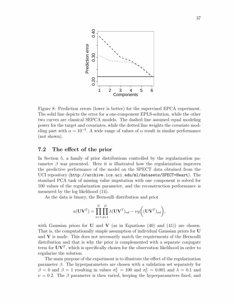
37

Components

Pre

dict

ion

erro

r1 2 3 4 5 6

0.20

0.30

0.40

Figure 8: Prediction errors (lower is better) for the supervised EPCA experiment.The solid line depicts the error for a one-component EPLS-solution, while the othertwo curves are classical SEPCA models. The dashed line assumed equal modelingpower for the target and covariates, while the dotted line weights the covariate mod-eling part with α = 10−3. A wide range of values of α result in similar performance(not shown).

7.2 The effect of the prior

In Section 5, a family of prior distributions controlled by the regularization pa-rameter β was presented. Here it is illustrated how the regularization improvesthe predictive performance of the model on the SPECT data obtained from theUCI repository (http://archive.ics.uci.edu/ml/datasets/SPECT+Heart). Thestandard PCA task of missing value imputation with one component is solved for100 values of the regularization parameter, and the reconstruction performance ismeasured by the log likelihood (14).

As the data is binary, the Bernoulli distribution and prior

a(UVT ) =N∏n=1

D∏d=1

λ(UVT )nd − νg(

(UVT )nd

),

with Gaussian priors for U and V (as in Equations (40) and (41)) are chosen.That is, the computationally simple assumption of individual Gaussian priors for Uand V is made. This does not necessarily match the requirements of the Bernoullidistribution and that is why the prior is complemented with a separate conjugateterm for UVT , which is specifically chosen for the observation likelihood in order toregularize the solution.

The main purpose of the experiment is to illustrate the effect of the regularizationparameter β. The hyperparameters are chosen with a validation set separately forβ = 0 and β = 1 resulting in values σ2

V = 100 and σ2U = 0.001 and λ = 0.1 and

ν = 0.2. The β parameter is then varied, keeping the hyperparameters fixed, and

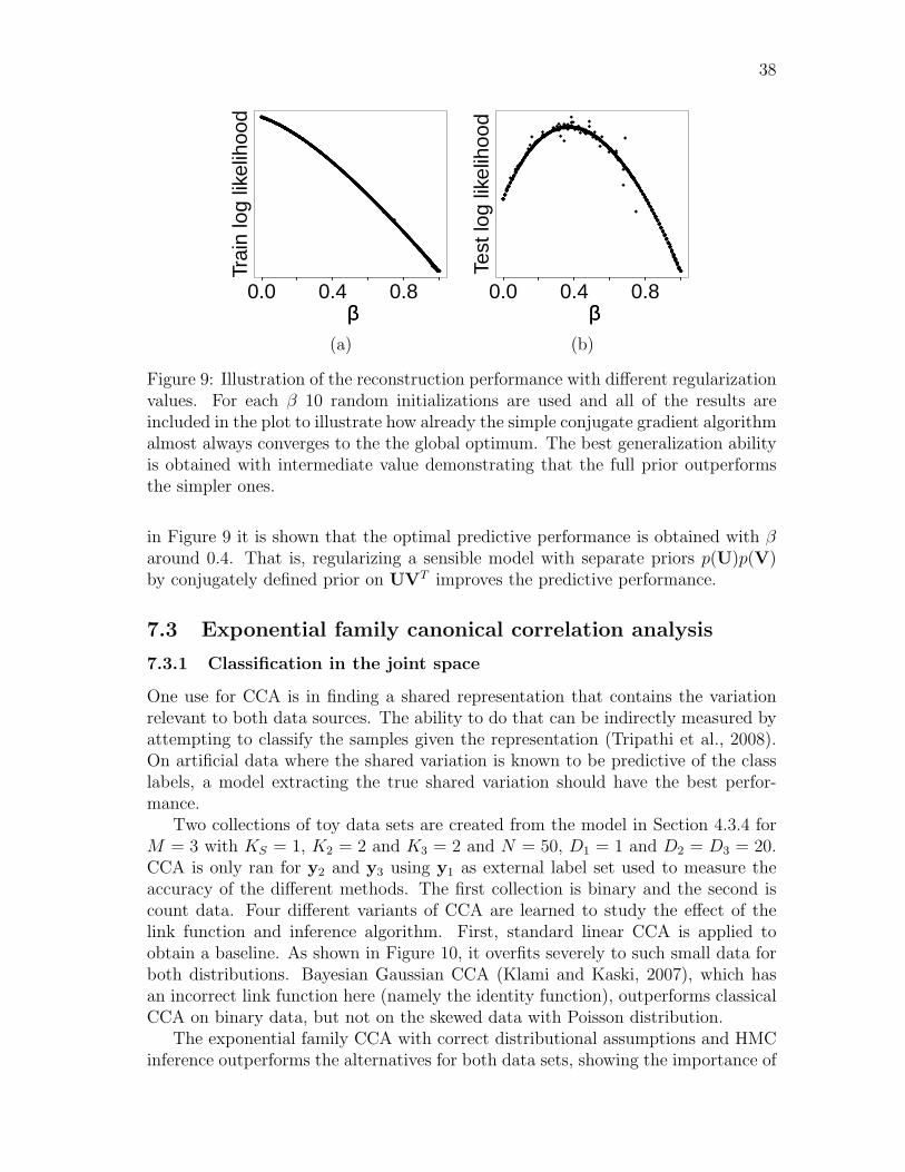
38

0.0 0.4 0.8

Trai

n lo

g lik

elih

ood

ββ0.0 0.4 0.8

Test

log

likel

ihoo

d

ββ(a) (b)

Figure 9: Illustration of the reconstruction performance with different regularizationvalues. For each β 10 random initializations are used and all of the results areincluded in the plot to illustrate how already the simple conjugate gradient algorithmalmost always converges to the the global optimum. The best generalization abilityis obtained with intermediate value demonstrating that the full prior outperformsthe simpler ones.

in Figure 9 it is shown that the optimal predictive performance is obtained with βaround 0.4. That is, regularizing a sensible model with separate priors p(U)p(V)by conjugately defined prior on UVT improves the predictive performance.

7.3 Exponential family canonical correlation analysis

7.3.1 Classification in the joint space

One use for CCA is in finding a shared representation that contains the variationrelevant to both data sources. The ability to do that can be indirectly measured byattempting to classify the samples given the representation (Tripathi et al., 2008).On artificial data where the shared variation is known to be predictive of the classlabels, a model extracting the true shared variation should have the best perfor-mance.

Two collections of toy data sets are created from the model in Section 4.3.4 forM = 3 with KS = 1, K2 = 2 and K3 = 2 and N = 50, D1 = 1 and D2 = D3 = 20.CCA is only ran for y2 and y3 using y1 as external label set used to measure theaccuracy of the different methods. The first collection is binary and the second iscount data. Four different variants of CCA are learned to study the effect of thelink function and inference algorithm. First, standard linear CCA is applied toobtain a baseline. As shown in Figure 10, it overfits severely to such small data forboth distributions. Bayesian Gaussian CCA (Klami and Kaski, 2007), which hasan incorrect link function here (namely the identity function), outperforms classicalCCA on binary data, but not on the skewed data with Poisson distribution.

The exponential family CCA with correct distributional assumptions and HMCinference outperforms the alternatives for both data sets, showing the importance of

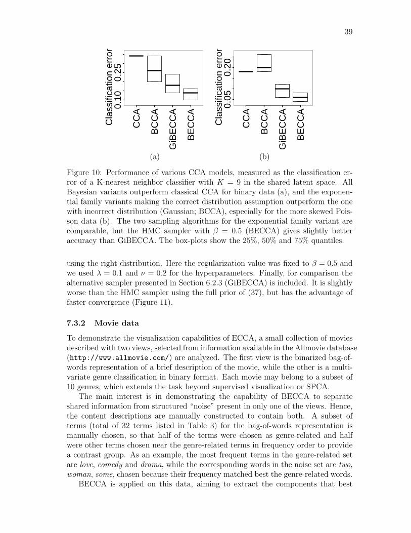
39

CC

A

BC

CA

GiB

EC

CA

BE

CC

A

0.10

0.25

Cla

ssifi

catio

n er

ror

CC

A

BC

CA

GiB

EC

CA

BE

CC

A

0.05

0.20

Cla

ssifi

catio

n er

ror

(a) (b)

Figure 10: Performance of various CCA models, measured as the classification er-ror of a K-nearest neighbor classifier with K = 9 in the shared latent space. AllBayesian variants outperform classical CCA for binary data (a), and the exponen-tial family variants making the correct distribution assumption outperform the onewith incorrect distribution (Gaussian; BCCA), especially for the more skewed Pois-son data (b). The two sampling algorithms for the exponential family variant arecomparable, but the HMC sampler with β = 0.5 (BECCA) gives slightly betteraccuracy than GiBECCA. The box-plots show the 25%, 50% and 75% quantiles.

using the right distribution. Here the regularization value was fixed to β = 0.5 andwe used λ = 0.1 and ν = 0.2 for the hyperparameters. Finally, for comparison thealternative sampler presented in Section 6.2.3 (GiBECCA) is included. It is slightlyworse than the HMC sampler using the full prior of (37), but has the advantage offaster convergence (Figure 11).

7.3.2 Movie data

To demonstrate the visualization capabilities of ECCA, a small collection of moviesdescribed with two views, selected from information available in the Allmovie database(http://www.allmovie.com/) are analyzed. The first view is the binarized bag-of-words representation of a brief description of the movie, while the other is a multi-variate genre classification in binary format. Each movie may belong to a subset of10 genres, which extends the task beyond supervised visualization or SPCA.

The main interest is in demonstrating the capability of BECCA to separateshared information from structured “noise” present in only one of the views. Hence,the content descriptions are manually constructed to contain both. A subset ofterms (total of 32 terms listed in Table 3) for the bag-of-words representation ismanually chosen, so that half of the terms were chosen as genre-related and halfwere other terms chosen near the genre-related terms in frequency order to providea contrast group. As an example, the most frequent terms in the genre-related setare love, comedy and drama, while the corresponding words in the noise set are two,woman, some, chosen because their frequency matched best the genre-related words.

BECCA is applied on this data, aiming to extract the components that best

40

0 10000 300001.

01.

52.

02.

53.

0

PS

RF

−va

lue

Number of samples

● ●

BECCAGiBECCA

Figure 11: Comparison of the sampling methods. The convergence of the two sam-plers is monitored by calculating the PSRF-values (Section 2.3) with 4 separatechains. The horizontal line corresponds to value 1.1 and the chain is converged ifthe value falls below that (Gelman et al., 2004). GiBECCA converges considerablyfaster than BECCA (approximately 20-fold difference). The figure also demonstratesthat if PSRF value is monitored too early it can give misleading results, because themovement of the BECCA sampler in the beginning is slow (PSRF values smallerthan 1.1).

capture the genre variation. The GiBECCA inference method (Algorithm 2) is usedbecause interpreting the actual components is easier in that model, and becauseit was found out to be nearly as good as HMC with the full prior in the previousexperiment while being much faster to compute. Figure 12 shows the first two sharedprojection vectors, that is, the first two columns of V. It is immediately noticed howthe part covering the noise-terms in VS2 is around zero for all terms, showing thatthe shared components do not capture description-specific noise. At the same time,each projection picks a subset of genre-related terms and actual genre memberships.Closer inspection of the features reveals that the first component separates romanticmovies from action movies, while the second component mainly separates family-targeted genres (cartoons, family movies) from drama.

41

Table 3: Features of movie data set.

Genres Genre-related Genre-independentdescriptions descriptions

action love twoanimation comedy womanart foreign drama some

classic death brothercomedy relationship nowdrama war formerfamily police littlehorror romantic still

romance violent headthriller beautiful involved

action townmarriage keep

crime fewescape working

romance offerthriller meanwhile

42

action

thriller

violentescapethriller

romance

romanticmarriage

art foreigndrama

drama

animation

family

comedy

(a) (b)

Figure 12: Illustration of the first two CCA components of the movie data. In bothfigures the top 10 bars represent the 10 genre membership indicators, the next 17bars the genre-related words in the textual description of the movie, and the bottom16 bars the genre-independent terms. Genre-related terms are present in the projec-tions much more strongly than the genre-independent ’noise’-terms, as they should.The first shared component (a) picks most genre-related terms, detecting a stronglink between the genre memberships and the descriptions. The second shared com-ponent (b) extracts a more detailed relationship: family/comedy/animation moviesare separated from the rest by absence of the word drama in the descriptions.

43

8 Discussion

Exponential family generalization of principal component analysis (EPCA) is anactive research area with recent publications published in the top machine learningconferences (Collins et al., 2002; Gordon, 2002; Guo and Schuurmans, 2008; Guo,2009; Mohamed et al., 2009; Sajama and Orlitsky, 2004; Schein et al., 2003; Singhand Gordon, 2008; Rish et al., 2008; Tipping, 2001). In this thesis, a general frame-work for matrix factorizations or projection methods in the exponential family waspresented by building on EPCA. It was described how various methods for analyzingpaired data sources can be derived from the general model by simple restrictions onthe projection vectors. As practical examples the first Bayesian exponential familyvariants of partial least squares and canonical correlation analysis were presented,opening up possibilities for applying basic tools for varying data types in a prin-cipled way. It was also shown how straightforward prior assumptions may lead topoor performance in exponential family models, and a regularizing prior was givento overcome the problems. Furthermore, inference methods were discussed for themodels demonstrating the variants on both artificial and real life data. The newsampling algorithm presented in this thesis, was shown to be much faster than theprevious approach (Mohamed et al., 2009) but slightly less accurate.

However, there is still work to be done: There are not yet good methods forinferring hyperparameters of the regularizing prior (which makes also model com-plexity selection difficult), and there remain open challenges in how to effectively doinference for CCA-like models with explicit noise components. For Gaussian modelsthe inference is efficient due to analytical marginalization, whereas other distribu-tions are still lacking efficient algorithms. A solution that utilizes the marginalizedvariant as a part of the process was proposed, but it is only applicable for a specialcase of our general prior family.

44

References

Archambeau, C. and Bach, F. (2009). Sparse probabilistic projections. In Advancesin Neural Information Processing Systems 21, pp. 73–80, Cambridge, MA, MITPress.

Archambeau, C., Delannay, N. and Verleysen, M. (2006). Robust probabilistic pro-jections. Proceedings of the 23rd International Conference on Machine Learning,pp. 33–40, New York, ACM press.

Bach, F. R. and Jordan, M. I. (2005). A probabilistic interpretation of canonicalcorrelation analysis. Technical Report 688, Department of Statistics, Universityof California, Berkeley.

Bach, F. R. and Jordan, M. I. (2002). Kernel independent component analysis.Journal of Machine Learning Research, 3:1–48.

Barber, D. and Williams, C. K. (1997). Gaussian processes for Bayesian classificationvia hybrid Monte Carlo. In: Advances in Neural Information Processing Systems9, pp. 340-346, Cambridge, MA, MIT Press.

Bingham, E., Kaba¡n, A. and Fortelius, M. (2009). The aspect Bernoulli model: mul-tiple causes of presences and absences. Pattern Analysis Applications, 12(1):55-78

Bishop, C.M. (2006). Pattern recognition and machine learning. Springer, NewYork.

Bernardo, J.M. and Smith, A.F (2000). Bayesian theory, Wiley, Chichester.

Bo, L. and Schimsesku, C (2009). Supervised spectral latent variables models.In Proceedings of the 12th Conference on Artificial Intelligence and Statistics,Florida, USA, JMLR:W&CP 5:33-39.

Collins, M., Dasgupta, S., and Schapire, R. E. (2002). A generalization of principalcomponents analysis to the exponential family. In Advances in Neural InformationProcessing Systems 14, pp. 617–624. Cambridge, MA, MIT Press.

Caruana, R. (1997). Multitask learning. Machine Learning, 28:41-75.

Gelman, A., Carlin, J.B., Stern, H.S. and Rubin, D.B. (2004). Bayesian data analysis(2nd edition). Chapman & Hall, Boca Raton FL.

Farquhar, J. D. R., Hardoon, D. R., Meng, H., Shawe-Taylor, J., and Szedmak, S.(2006). Two view learning: SVM-2K, theory and practice. In Advances in NeuralInformation Processing Systems 18, pp. 355–362, Cambridge, MA, MIT Press.

Gordon, G. (2002). Generalized2 linear2 models In Advances in Neural InformationProcessing Systems 15, pp. 577–584. Cambridge, MA, MIT Press.

45

Guo, Y. (2009). Supervised exponential family principal component analysis viaconvex optimization. In Advances in Neural Information Processing Systems 21,pp. 569–576. Cambridge, MA, MIT Press.

Guo, Y. and Schuurmans, D. (2008). Efficient global optimization for exponen-tial family PCA and low-rank matrix factorization. In Allerton Conference onCommunications, Control, and Computing, pp. 1100–1107. IEEE.

Gustafsson, M. G. (2001). A probabilistic derivation of the partial least-squaresalgorithm. Journal of Chemical Information and Modeling, 41:288–294.

Heller, K.A., Williamson, S. and Ghahramani, Z. (2008). Statistical models for Par-tial membership. In Proceedings of the 25th International Conference on MachineLearning, pp. 392–399, New York, ACM.

Hoff, P. D. (2007). Model averaging and dimension selection for the singular valuedecomposition. Journal of the American Statistical Association, 102:674–685.

Hoff, P. D. (2007). Simulation of the matrix Bingham-Von Mises-Fisher distribution with applications to multivariate and relational data,http://arxiv.org/pdf/0712.4166v1.

Hotelling, H. (1933). Analysis of a complex of statistical variables into principalcomponents. Journal of Educational Psychology, 24:417–41, 498–520.

Hotelling, H. (1936). Relations between sets of variates. Biometrika, 38:321–377.

Jolliffe, I.T. (1986). Principal component analysis. Springer-Verlag, New York.

Klami, A. and Kaski, S. (2007). Local dependent components. In Proceedings ofthe 24th International Conference on Machine Learning, pp. 425–432. Omnipress,Madison, WI.

Klami, A. and Kaski, S. (2008). Probabilistic approach to detecting dependenciesbetween data sets. Neurocomputing, 72:39–46.

Lawrence, N. (2005). Probabilistic non-linear principal component analysis withGaussian process latent variable models. Journal of Machine Learning Research,6:1783–1816.

Lee, D.D. and Seung, H.S. (2001). Algorithms for non-negative matrix factoriza-tion. In Advances in Neural Information Processing Systems 13, pp.556–562,Cambridge, MA, MIT press.

Lian, H. (2009). Bayesian nonlinear principal component analysis using randomfields. IEEE Transactions on Pattern Analysis and Machine Intelligence, 31: 749–754.

46

Ma H., Yang H., Lyu M.R. and King I. (2008). SoRec: Social recommendation usingprobabilistic matrix factorization Proceedings of 17th Conference on Informationand Knowledge Management, pp. 931–940, New York, ACM.

MacKay, D.J. (2002). Information theory, inference & learning algorithms. Cam-bridge University Press.

Mohamed, S., Heller, K., and Ghahramani, Z. (2009). Bayesian exponential familyPCA. In Advances in Neural Information Processing Systems 21, pp. 1089–1096.Cambridge, MA, MIT Press.

Neal R.M. (1993). Probabilistic inference using Markov Chain Monte Carlo meth-ods. Tech. Report CRG-TR-93-1,University of Toronto, Department of ComputerScience.

Neal, R. M. (1996). Bayesian learning for neural networks. Springer-Verlag, NewYork.

Nounou, M., Bakshi, B., Goel, P., and Shen, X. (2002). Process modeling byBayesian latent variable regression. AIChE Journal, 48:1775–1793.

Pearson, K. (1901). On lines and planes of closest fit to the systems of points inspace. Philosophical Magazine, 2:559-572.

Rish, I., Grabarnik, G., Cecchi, G., Pereira, F., and Gordon, G. J. (2008). Closed-form supervised dimensionality reduction with generalized linear models. In Pro-ceedings of the 25th International Conference on Machine Learning, pp. 832–839,New York, NY, ACM.

Roweis, S. and Ghahramani, Z. (1999). A unifying review of linear Gaussian models.Neural Computation, 11:305–345.

Sajama and Orlitsky, A. (2004). Semi-parametric exponential family PCA. In Ad-vances in Neural Information Processing Systems 17, pp. 1177–1184, Cambridge,MA, MIT Press.

Salakhutdinov R. and Mnih A. (2008). Probabilistic matrix factorization. In Ad-vances in Neural Information Processing Systems 20. Cambridge, MA, MIT Press.

Salakhutdinov R. and Mnih A. (2008) (b). Bayesian probabilistic matrix factoriza-tion using Markov Chain Monte Carlo. InProceedings of the 25th internationalconference on Machine learning, pp. 880-887, New York, ACM.

Schein A.I, Saul L.K., and UngarL.H. (2003). A generalized linear model for princi-pal component analysis of binary data. In Proceedings of the Ninth InternationalWorkshop on Artificial Intelligence and Statistics,

Shawe-Taylor, J. and Cristianini, N. (2004). Kernel methods for pattern recognition,Cambridge University Press.

47

Singh, A.P. and Gordon, G.J. (2008). Relational learning via collective matrixfactorization. Proceedings of the 14th ACM SIGKDD International Conferenceon Knowledge Discovery and Data Mining, pp.650-658, New York, ACM.

Srebro, N. and Jaakkola, T. (2003). Weighted low-rank approximations. In Pro-ceedings of the 20th International Conference on Machine Learning, pp. 720-727.USA, AAAI Press.

Tipping, M.E. (2001). Probabilistic visualization of high-dimensional binary dataIn Neural Information Processing Systems 11, pp.592-598, Cambridge, MA, MITPress.

Tipping, M. and Bishop, C. (1999). Mixtures of probabilistic principal componentanalyzers. Neural Computation, 11:443–482.

Tripathi, A.., Klami, A., and Kaski, S. (2008). Simple integrative preprocessingpreserves what is shared in data sources. BMC Bioinformatics 2008, 9:111

Vinokourov, A., Christianini, N., and Shawe-Taylor, J. (2003). Inferring a semanticrepresentation of text via cross-language correlation analysis. In Advances inNeural Information Processing Systems 15, pp. 1473–1480. Cambridge, MA, MITPress.

Williamson, S and Ghahramani, Z. (2008). Probabilistic models for data combi-nation in recommender systems. In Advances in Neural Information ProcessingSystems 20 Workshop: Learning from Multiple Sources

Yu, S., Yu, K., Tresp, V., Kriegel, H.-P., and Wu, M. (2006). Supervised probabilisticprincipal component analysis. In Proceedings of the 30th annual InternationalACM SIGIR Conference on Knowledge Discovery and Data Mining, pp. 464–473.New York, NY, ACM Press.