Augmentation and Evaluation of Training Data forDeep Learning

Junhua DingDepartment of Computer Science

East Carolina UniversityGreenville, NC, USA

dingj@ecu.edu

XinChuan LiSchool of Computer Science

China University of GeosciencesWuhan, China

lihanyu2006@foxmail.com

Venkat N. GudivadaDepartment of Computer Science

East Carolina UniversityGreenville, NC, USAgudivadav15@ecu.edu

Abstract—Deep learning is an important technique for ex-tracting value from big data. However, the effectiveness of deeplearning requires large volumes of high quality training data.In many cases, the size of training data is not large enough foreffectively training a deep learning classifier. Data augmentationis a widely adopted approach for increasing the amount oftraining data. But the quality of the augmented data maybe questionable. Therefore, a systematic evaluation of trainingdata is critical. Furthermore, if the training data is noisy, it isnecessary to separate out the noise data automatically. In thispaper, we propose a deep learning classifier for automaticallyseparating good training data from noisy data. To effectivelytrain the deep learning classifier, the original training data needto be transformed to suit the input format of the classifier.Moreover, we investigate different data augmentation approachesto generate sufficient volume of training data from limited sizeoriginal training data. We evaluated the quality of the trainingdata through cross validation of the classification accuracy withdifferent classification algorithms. We also check the patternof each data item and compare the distributions of datasets.We demonstrate the effectiveness of the proposed approachthrough an experimental investigation of automated classificationof massive biomedical images. Our approach is generic and iseasily adaptable to other big data domains.

Keywords-big data; machine learning; neural network; deeplearning; convolutional neural network; support vector machine;diffraction image

I. INTRODUCTION

Scalable and high performance data processing infrastruc-ture and analytics tools are needed to extract value frombig data. For example, deep learning algorithms and GPUshave been widely adopted for analyzing big data [1]. Achallenging factor for effectively extracting value from bigdata is its size and quality. Furthermore, the data availablefor training algorithms such as a deep learning classifier isoften not large enough. Augmenting data through methodssuch as transforming existing data items into new ones isa widely used practice. However, it is difficult to determinewhether or not the augmented data is valid. It is necessaryto systematically evaluate the quality of the generated datathrough transformations. Also, the generated training data mayinclude noise in the form of, for example, mislabeled data.

Published research has shown that anomalies and noise intraining datasets could significantly decrease the performance

and accuracy of data analysis [2] [3]. To address these prob-lems, we have two choices: devise robust machine learningalgorithm which can deal with noisy training data, or improvethe quality of the data through filtering [4].

Both general purpose and domain-specific techniques andtools have been developed for quality assurance of big data.Gao et al. provides an overview of issues, challenges andtools for validation and quality assurance of big data [5]. Theydefine big data quality assurance as the study and applicationof quality assurance techniques and tools to ensure the qualityattributes of big data. Web is one primary source of big data,and work on the evaluation of the veracity of web sourcesexists in the literature.

Machine learning algorithms have been used for detectingduplicates in data that originated from multiple sources [6].Data filtering is an approach for improving data qualitythrough noise removal. Data publishers and subscribers canfilter noisy data using domain models and rules [7]. Due tothe massive scale of big data, automated filtering of data isessential. However, investigations in this direction are justbeginning to appear.

In this paper, we introduce a systematic approach forseparating noisy data from biomedical image datasets to enableextraction of knowledge from big data. More specifically,we develop a machine learning approach for separating bothinvalid and noisy data from a dataset. Our approach includesan iterative process for separating noisy data from regular datausing a deep learning classifier. We also discuss an approachto generating large volume of high quality data for improvingclassification accuracy. To ensure the quality of the augmenteddata, we evaluate data quality through cross validation ofclassification accuracy with different classification algorithms.We also check the pattern of each data item and compare theirdistributions.

We describe the proposed approach and demonstrate itseffectiveness through separating the diffraction images ofbiology cells into several categories including noisy class.Diffraction images of cells are acquired using a polarizationdiffraction image flow cytometer (p-DIFC), which is used forquantifying and profiling 3D morphology of single cells [8].The 3D morphological features of a cell that are captured inthe diffraction image are used for accurately classifying cell

types. p-DIFC can take the diffraction images of nearly 100cells per second. Using p-DIFC, we have collected over amillion diffraction images for different types of cells.

II. CELL DIFFRACTION IMAGES

Work on classification of cell diffraction images usingmachine learning has been reported in the literature. However,p-DIFC imaging may include lots of non-cell particles such asghost cell body, aggregated spherical particles (aka fracturedcells), and cell debris and small particles (collectively referredto as debris). We refer to the viable cells with intact structuresas cells. The diffraction images taken from the non-cellparticles are also collected into the diffraction image dataset.The diffraction images of the non-cell particles comprise thenoise data.

To accurately classify cells, it is necessary to separatethe non-cell diffraction images (i.e., the noise) from the celldiffraction images. Manually separating the noise images fromcell images is not feasible from a practical standpoint. Toaddress this issue, we developed a deep learning [1] approachfor automated classification of diffraction images. We classifythe diffraction images into three categories: cells, fracturedcells, and debris. We developed the classifier using a deeplearning architecture based on AlexNet [9] and TensorFlowframeworks. We trained the classifier using diffraction imagesof cells, fractured cells, and debris.

The size of a raw 8-bit gray scale p-DIFC diffraction imageis 640× 480 pixels. Since AlexNet works with images of size227×227 pixels, we resized the original diffraction images to227 × 227. AlexNet classifier for diffraction images requiresa large volume of training images. We developed an approachfor generating several small diffraction images (aka augmenteddiffraction images) from the original images. The classificationaccuracy is cross checked with n-fold cross validation (NFCV)and a confusion matrix.

To check the quality of the training data, we developeda support vector machine (SVM) for classifying the threecategories of diffraction images. First, we train the classifieron the original and the augmented diffraction image datasetsseparately. Next, we compare the classification accuracies. Wealso investigate whether the small images can capture enoughmorphology information as the original images. We requireeach small image to be different from its original image.Furthermore, we desire that all the small images which aregenerated from the same original to exhibit different textualpatterns. Lastly, we check the distribution of selected featurevalues of the original and the augmented datasets to determinewhether they are consistent.

The remainder of this paper is organized as follows. Section2 provides the domain background in cell imaging and auto-mated classification of diffraction images. Section 3 describesan approach for systematically evaluating the quality of aug-mented iamge datasets. Related work is discussed in Section4 and Section 5 concludes the paper.

Fig. 1. (A). Light scattering schema of p-DIFC, (B).Software simulateddiffraction images, and (C). p-DIFC acquired diffraction images.

III. AUTOMATED CLASSIFICATION OF DIFFRACTIONIMAGES

We first discuss morphology based cell classification. Next,we introduce automated classification of diffraction imagesusing SVM and deep learning techniques.

A. Morphology Based Cell Classification

Cells exhibit highly varied and convoluted 3-dimensional(3D) structures through intracellular organelles to sustainphenotypic variations and functions. Cell classification is im-portant to biology and life science research. Morphology basedapproaches at the single cell-level is attracting intense researchefforts for their direct relations to cellular functions. p-DIFCis used to rapidly acquire cross-polarized Diffraction Image(p-DI) pairs from single cells [8]. It adopts Stokes vectorsand Mueller matrices to account for the polarization changein scattered light as a result of intracellular distribution ofrefractive index, n(r, λ), or its 3D morphology. The incidentlight and its polarization state is represented by Stokes vector(I0, Q0, U0, V0), which propagates along the z-axis. Likewise,the scattered light and its polarization is represented statevector (Is, Qs, Us, Vs) along (Θs,Φs) direction, as shownin Fig. 1. Different from images acquired by non-coherentlight, the p-DI pairs present characteristic patterns due to thecoherent light scatter emitted by the intracellular moleculardipoles induced by an incident laser beam [8]. The p-DI datathus provide a data source to probe the 3D morphology of theilluminated cells that requires machine learning techniques forextracting morphological and molecular information.

During the last decade, Ding et al. have developed differentmachine learning approaches, including Support Vector Ma-chine (SVM) [10] and deep learning, for rapid and accuratecell morphology analysis of cell diffraction images [3] [11][12].

B. Datasets

A collection of diffraction images acquired using p-DIFCmay include images taken from non-regular cells especiallyfractured cells and debris in the samples. For some research

(a) (b) (c)

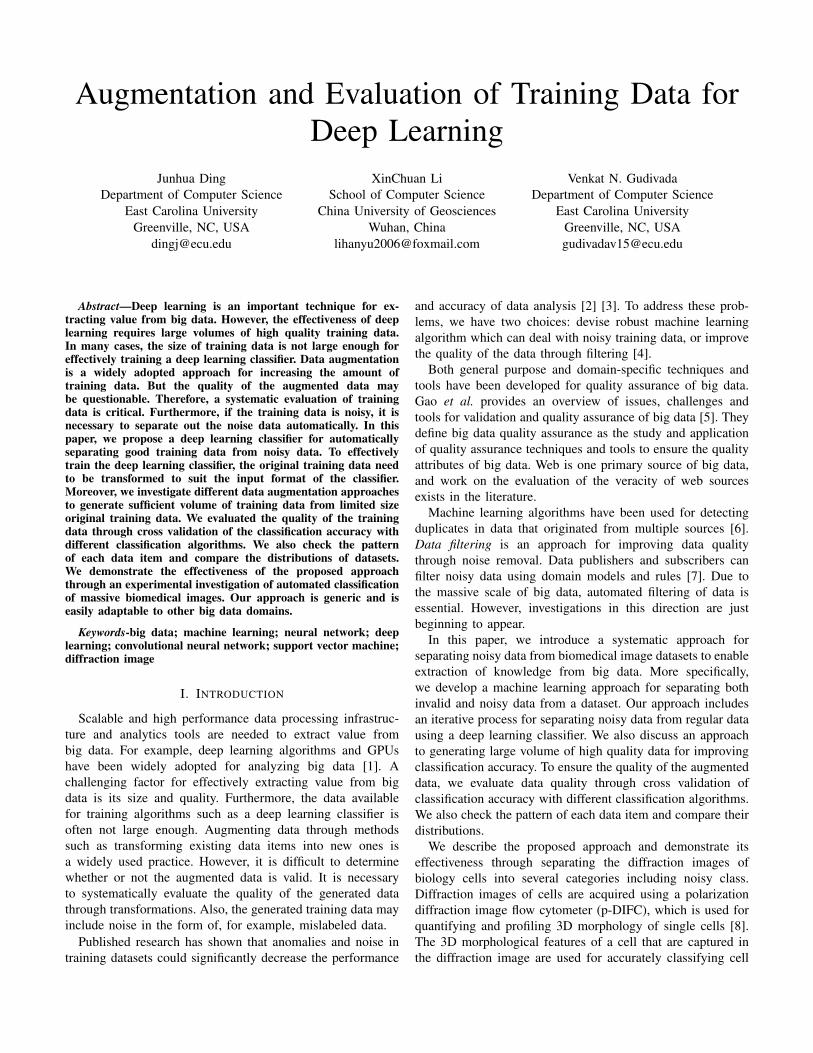
Fig. 2. A p-DIFC acquired diffraction image of (a) a viable cell of intactstructure, (b) a ghost cell body or aggregated spherical particles, and (c) acell debris or small particle. The top right corner shows the correspondingparticle of each image.

projects, one needs only normal cell images. For some otherresearch such as apoptosis study, we need only fractured cellimages. Therefore, it is necessary to build a tool to automatethe separation of the three types of diffraction images.

The three types of cell particles have different morphologystructures that are precisely captured in p-DIFC diffractionimages. Using these textual patterns, a biologist can separatethe three types of images visually. Fig. 2 shows thee samplep-DIFC diffraction images and their corresponding particles.The textual pattern of the diffraction image of a viable cell ofintact structure contains many bright normal speckles. On theother and, a ghost cell body or aggregated spherical particleincludes bright strips. Lastly, a cell debris or small particleshows many large diffuse speckles.

The difference in textual patterns of the three categoriesof diffraction images is good enough to separate the threecategories using machine learning algorithms. We acquiredmany diffraction images for the three categories of parti-cles using p-DIFC and then selected several thousands ofdiffraction images as the initial dataset. For the experimentalstudy, we selected a total of 7519 diffraction images. Eachdiffraction image was manually inspected and and its categorywas labeled. Normal cells are labeled as cells, fractured cells asstrips, and debris as simply debris. The initial image dataset iscomprised of 2232 normal cells, 1645 fractured cells, and 3642debris. Each category of the diffraction images is stored in aseparate directory. We note that some of the diffraction imagescould have been incorrectly labeled, whereas some others weredifficult to label due to low visual quality.

C. SVM-based Image Classification

An SVM performs binary classification in general [10]. Toimplement a multiclass classification, several SVM classifiersare combined by comparing ’one against the rest’ or ’oneagainst one’. We have implemented the classifier for diffrac-tion images using LIBSVM [13], which is an open-sourcetoolkit for SVM.

The textual pattern of the diffraction images is defined usinga group of Grey Layer Collaborative Matrix (GLCM) features[14]. We use a total of 20 features – 14 are features fromthe original image and 6 features from the extended images.The definition of each feature can be found in Ding’s previouswork [15]. The procedure of building an SVM classifier fordiffraction images is given below:

TABLE ICONFUSION MATRIX OF THE CLASSIFICATION OF DIFFRACTION IMAGES

Cells Debris StripsCells 74.50% 16.00% 9.50%Debris 6.50% 81.50% 12.00%Strips 14.00% 24.00% 62.00%

1) Calculate GLCM features for each diffraction image inthe training and testing datasets.

2) Label each diffraction image with its category such asits cell type, and build a feature vector consisting of itsGLCM feature values and its label. The feature vectorsof all diffraction images in a dataset form a featurematrix.

3) Train the SVM classifier using the select kernel and thefeature matrix of the training dataset.

4) Test the classifier with diffraction images in test dataset,and validate the classification performance using criteriasuch as N-fold Cross Validation (NFCV) and confusionmatrix.

We built an SVM classifier using the diffraction imagedataset. We selected 1000 diffraction images for each ofthe three classes, and built the feature matrix with GLCMfeature values and the corresponding types. Each feature vectorincludes 16 GLCM feature values since the value of onefeature is all 0s and another three features are defined on imageformat, which was not accounted for in this study. The averageclassification accuracy of 10 fold cross validation (10FCV)for cells, debris and strips is 74.50%, 81.50% and 62.00%,respectively. The simplified confusion matrix is shown in TableI [16].

To improve the classification accuracy of the SVM classifier,we have experimented with many different techniques such aspre-selecting the images using image processing and clusteranalysis techniques [3], and feature selection [17]. Our recentexperiments have shown that deep learning approaches greatlyimprove the classification accuracy [18].

D. Deep Learning Based Image Classification

Diffraction images are relatively simple due to their lowresolution and absence of background noise. Therefore, weselected AlexNet model [9] which is implemented in Tensor-Flow framework to build the deep learning classifier. As deeplearning requires a large number of features, the size of thetraining dataset is also large.

AlexNet is trained using about 1.2 million images. Wedid not use the pre-trained AlexNet, but used only its netarchitecture. We initially made some minor changes of thearchitecture of AlexNet such as changing the output of the lastfully connected layer from 1000 categories to 3, and removedsome convolutional layers. These changes neither improvedthe training performance or the classification accuracy. Toavoid the potential of introducing bugs, we decided to keepthe original AlexNet architecture in tact. We have collectedonly 7519 raw diffraction images, which are not large enough

for training AlexNet. Therefore, we used data augmentationapproaches for producing a larger volume training dataset.

E. Data Augmentation

The size of a raw diffraction image of a cell is 640×490 pix-els. It is large enough to be divided into several small imagesof size 227 × 227 pixels, which is the size of AlexNet inputimage. Each small image should contain sufficient informationto represent the original image according to p-DIFC principles[8]. If we check a diffraction image of a cell, it is not difficultto find the textual pattern is repeated in the image as shownin Fig. 2. Since the lens of the camera taking cell diffractionimage of cell has a different angle to each part of the cell,the textual pattern is not simply repeated in the image. Acarefully chosen sub-image can have enough information tobe a representative of the whole image. A diffraction imagemay also include large black background which is useless forclassification. Therefore, a rigorous approach for producingthe small images is necessary. This property can be furtherconfirmed by the diffraction images shown in Fig. 7, whichare produced by simulating the light scattering of scatterersusing aDDA (a light scattering simulation program) [19].

F. Cropping images

As noted earlier, AlexNet accepts input images of size227× 227 pixels. Also, the size of original diffraction imagesis 640 × 480 pixels. Therefore, a small image is about 1/5 ofthe size of the original image. Furthermore, since a diffractionimage may contain significant black area, the center of thetextual pattern such as bright speckles or strips may not bethe center of the image. We need find the center of thetextual pattern area to perform cropping, which is normallythe brightest area in the image.

Given a 5×5 pixel window, cropping program calculates theaverage intensity of the window. Then it slides the window byseveral pixels in steps to cover the whole image, to determinea window that has the largest average intensity. For example,the intensity range of a 8-bit resolution image is from 0 to255. The window with the largest average intensity is set asthe center for cropping small images. If multiple windowshave the largest average intensity, then the one furthest to theboundary is selected as the center. A small image is croppedfrom the original image around the center first, and then moresmall images are cropped through sliding the window fromthe center some pixels in any direction as shown in Fig. 3.

Fig. 3. An Illustration ofImage Cropping

In our study, the 227 × 227-pixelwindow is moved from the center in8 different directions and the angleθ between two adjacent directions is45o. The sliding window moves dpixels from last window in a direc-tion and crops a new small image.The moving distance d ranges from7 to 17 pixels. However, other d val-ues may also work well. The sliding

window can be moved in one direc-tion several steps to crop multiplesmall images in that direction. Whena sliding window is moved to a new position, it is necessaryto ensure that the entire sliding window is still contained inthe original image boundary. If not, the window is discardedand no further sliding in that direction takes place. Using theapproach, we generated 56 small images from a normal cellimage with a step distance d of 11 pixels (which means sliding11 pixels 7 times in each direction), 40 images from a debrisimage with d as 14, and 72 images from a strips image withd as 9.

The small image generation via cropping is fully automatedwith a python program. Though the multiple small imagescropped from the same image are different from each other,but they all represent the same original image and are labeledas the same category as that of the original image. Finally,105291 small diffraction images of cells, 127733 small diffrac-tion images of debris, and 92767 small diffraction images ofstrips are selected for training the deep learning classifier.

G. Pooling Images

Cropping technique does not work for the case where thewhole image is critical for classification. In such cases, localfeatures that are extracted from a local area are not enough torepresent the global features extracted from the whole image.A different technique is needed for producing the training datafrom the limited number of original images. We experimenteda pooling technique for producing large volume of trainingdata. A raw diffraction image is downsampled into a smallimage using pooling. Multiple small images can be producedfrom a raw image with different pooling configurations. Also,small images can be produced with different pooling functionssuch max pooling or average pooling [20].

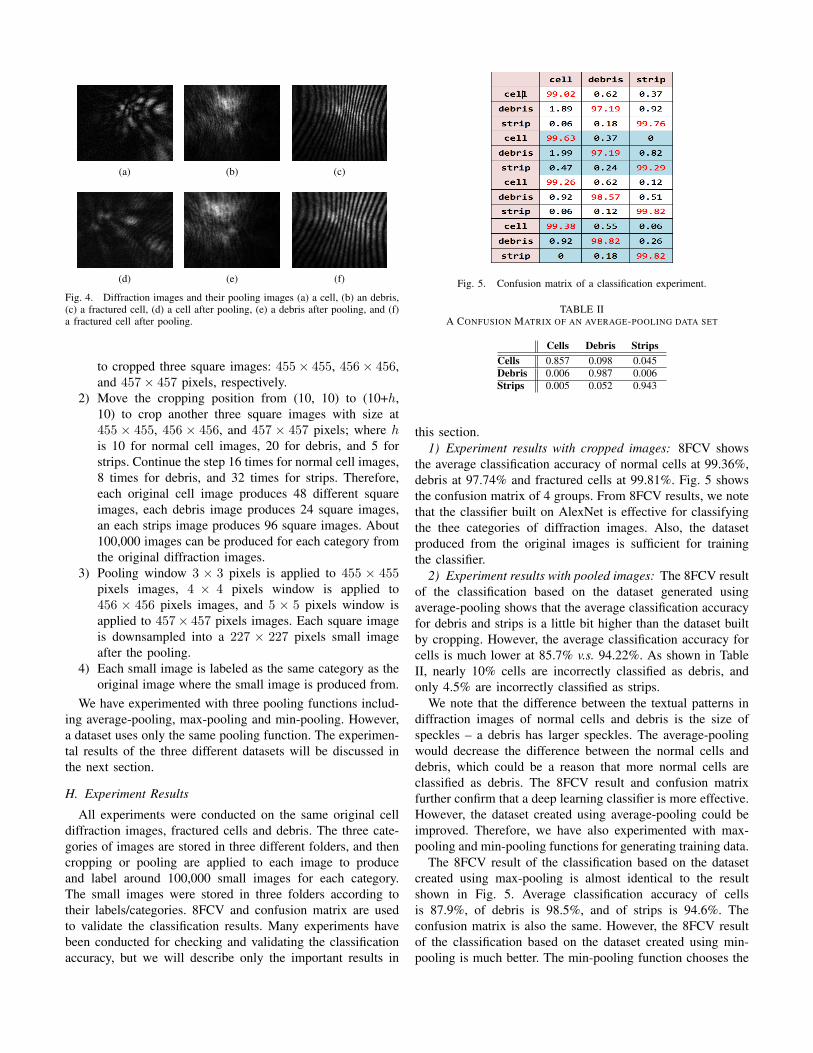
To produce multiple small diffraction images from oneoriginal image, we apply different pooling window sizes anddifferent sliding stride to the same image. Since the size of thesmall image is 227 × 227 pixels, and the size of an originalimage is 640 × 480 pixels, we resize the original image intoa square one. We cut three different size squares from animage, which are 455×455, 456×456, and 457×457 pixels.Next, 3 × 3, 4 × 4, and 5 × 5 pooling windows are appliedto these three squares. The stride distance is set to 2 pixels.The size of the output image from the pooling is s ∗ s pixels,s = (x − m)/c + 1, where x × x pixels are the size of theinput image of the pooling, m×m pixels are the size of thepooling window, and c is the stride distance. For example, ifthe input image is 455× 455, pooling window is 3× 3 pixels,and stride distance is 2, the size of the output image will be227 × 227 pixels. Fig. 4 shows a comparison of the originalimages and their pooling images (the ratio of the images werechanged due to formatting issues). It clearly shows that thetextual patterns of the original image are well preserved in thepooling image. The pooling steps are:

1) For each diffraction image, select position (10, 10) ofthe image as position (0, 0) of the new cropped images

(a) (b) (c)

(d) (e) (f)

Fig. 4. Diffraction images and their pooling images (a) a cell, (b) an debris,(c) a fractured cell, (d) a cell after pooling, (e) a debris after pooling, and (f)a fractured cell after pooling.

to cropped three square images: 455 × 455, 456 × 456,and 457 × 457 pixels, respectively.

2) Move the cropping position from (10, 10) to (10+h,10) to crop another three square images with size at455 × 455, 456 × 456, and 457 × 457 pixels; where his 10 for normal cell images, 20 for debris, and 5 forstrips. Continue the step 16 times for normal cell images,8 times for debris, and 32 times for strips. Therefore,each original cell image produces 48 different squareimages, each debris image produces 24 square images,an each strips image produces 96 square images. About100,000 images can be produced for each category fromthe original diffraction images.

3) Pooling window 3 × 3 pixels is applied to 455 × 455pixels images, 4 × 4 pixels window is applied to456 × 456 pixels images, and 5 × 5 pixels window isapplied to 457 × 457 pixels images. Each square imageis downsampled into a 227 × 227 pixels small imageafter the pooling.

4) Each small image is labeled as the same category as theoriginal image where the small image is produced from.

We have experimented with three pooling functions includ-ing average-pooling, max-pooling and min-pooling. However,a dataset uses only the same pooling function. The experimen-tal results of the three different datasets will be discussed inthe next section.

H. Experiment Results

All experiments were conducted on the same original celldiffraction images, fractured cells and debris. The three cate-gories of images are stored in three different folders, and thencropping or pooling are applied to each image to produceand label around 100,000 small images for each category.The small images were stored in three folders according totheir labels/categories. 8FCV and confusion matrix are usedto validate the classification results. Many experiments havebeen conducted for checking and validating the classificationaccuracy, but we will describe only the important results in

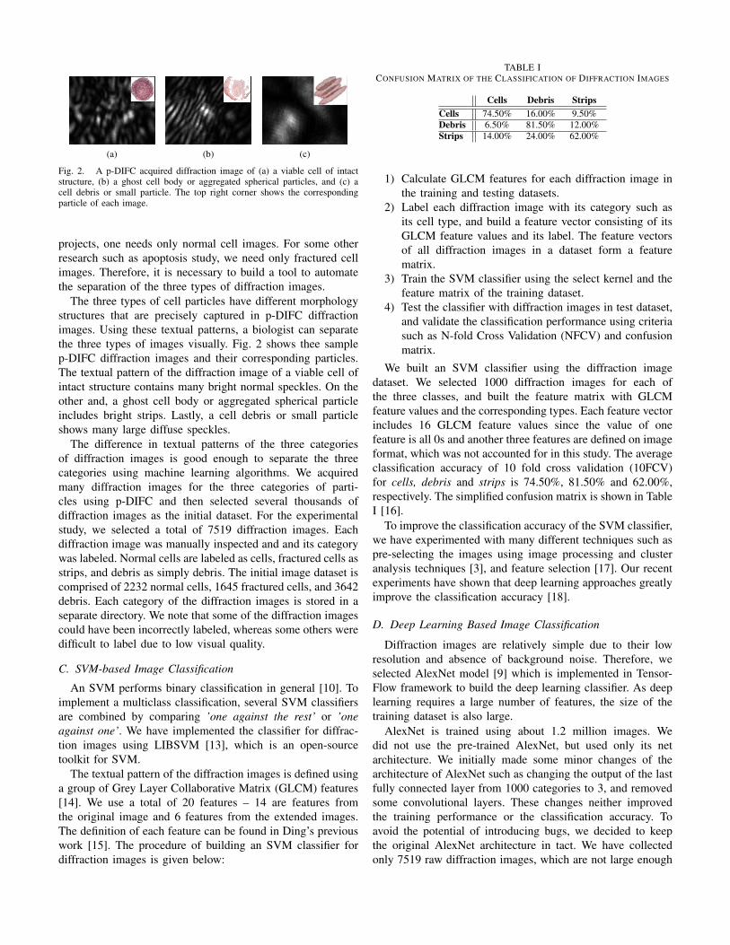
Fig. 5. Confusion matrix of a classification experiment.

TABLE IIA CONFUSION MATRIX OF AN AVERAGE-POOLING DATA SET

Cells Debris StripsCells 0.857 0.098 0.045Debris 0.006 0.987 0.006Strips 0.005 0.052 0.943

this section.1) Experiment results with cropped images: 8FCV shows

the average classification accuracy of normal cells at 99.36%,debris at 97.74% and fractured cells at 99.81%. Fig. 5 showsthe confusion matrix of 4 groups. From 8FCV results, we notethat the classifier built on AlexNet is effective for classifyingthe thee categories of diffraction images. Also, the datasetproduced from the original images is sufficient for trainingthe classifier.

2) Experiment results with pooled images: The 8FCV resultof the classification based on the dataset generated usingaverage-pooling shows that the average classification accuracyfor debris and strips is a little bit higher than the dataset builtby cropping. However, the average classification accuracy forcells is much lower at 85.7% v.s. 94.22%. As shown in TableII, nearly 10% cells are incorrectly classified as debris, andonly 4.5% are incorrectly classified as strips.

We note that the difference between the textual patterns indiffraction images of normal cells and debris is the size ofspeckles – a debris has larger speckles. The average-poolingwould decrease the difference between the normal cells anddebris, which could be a reason that more normal cells areclassified as debris. The 8FCV result and confusion matrixfurther confirm that a deep learning classifier is more effective.However, the dataset created using average-pooling could beimproved. Therefore, we have also experimented with max-pooling and min-pooling functions for generating training data.

The 8FCV result of the classification based on the datasetcreated using max-pooling is almost identical to the resultshown in Fig. 5. Average classification accuracy of cellsis 87.9%, of debris is 98.5%, and of strips is 94.6%. Theconfusion matrix is also the same. However, the 8FCV resultof the classification based on the dataset created using min-pooling is much better. The min-pooling function chooses the

TABLE IIIA CONFUSION MATRIX OF A MIN-POOLING DATA SET

Cells Debris StripsCells 0.935 0.036 0.030Debris 0.024 0.961 0.015Strips 0.023 0.044 0.933

minimal value of the sliding window to represent the wholewindow in the new image. The average classification accuracyof cells is improved to 93.5%, of debris to 96.1%, and offractured cells to 93.3%. The confusion matrix is shown inTable III. Fig. 6 shows a comparison of the average-poolingimages and their corresponding min-pooling images. We foundthat the textual patterns in min-pooling images are clearer,which might explain the improvement in the classificationaccuracy.

I. Discussion

In this section, we discuss how machine learning classifiersfor separating noise data from training data are built. We alsodemonstrate its process and effectiveness through classifyingthree categories of diffraction images. Through separatingfractured cell images and debris images from the trainingdata, one can get noise-free cell images that are importantfor training a classifier. However, the classification accuracyof an SVM based classifier is not high enough. Therefore, webuilt the deep learning classifier. Training the deep learningclassifier needs a large amount of high quality training data.Different data augmentation approaches including croppingand pooling are experimented for producing the needed data.

Our experimental results show that a deep learning classifieris highly effective, which can be used for automated selectionof data from a large dataset and filtering noise data. The qualityof dataset can be iteratively improved through multiple roundsof selection, in which the incorrectly classified data items fromprevious round of classification were inspected and re-labeledor removed for next round of training and classification. Sincethe quality of the training data is key to the quality the deeplearning classifier, it is important to evaluate the quality ofthe augmented dataset in term of representativity, fidelity andvariety. A high quality augmented dataset should have high arepresentativity, fidelity, and variety.

IV. EVALUATION OF THE QUALITY OF AUGMENTED DATA

In this section, we discuss how to systematically evaluate thequality of datasets that are produced from original diffractionimages using cropping or pooling techniques. We evaluatethe dataset using representativity, fidelity, and variety. Rep-resentativity means that the dataset includes all information inthe original dataset and it can represent the original datasetto train a machine learning classifier. Fidelity refers to thefact that a generated data item cannot be distinguished fromthe original source. Variety means the augmented datasetshould be normally distributed for non-trivial features. Forthe diffraction image case study, we first checked whether thesmall size diffraction images can be used for classifying the

TABLE IVCONFUSION MATRIX OF AN SVM BASED CLASSIFICATION OF

AUGMENTED DATA

Cells Debris StripsCells 77.94% 10.97% 11.09%Debris 7.33% 84.39% 8.28%Strips 20.25% 18.69% 61.06%

diffraction images based on SVM algorithm to achieve thesimilar accuracy as the original images. Then we checked thetextual pattern of the small images to ensure the small imagecan capture enough morphology information as its originalimage. Finally, we compared the distribution of feature valuesof the augmented data set and the original image data set.

A. Checking the classification accuracy of the SVM classifier

Table I shows a confusion matrix of the classification ofdiffraction images using an SVM classifier which is trainedusing the original diffraction image datasets. We check theclassification accuracy of the classifier based on the generateddiffraction images. We trained the SVM classifier using thedataset consisting of the small diffraction images producedby cropping or pooling from the original diffraction images.These are the images that are also used for training theclassifier shown in Table I. We select 3000 small imagesfor each category and then conduct an 8FCV. The confusionmatrix of the average result of 8FCV is shown in TableIV. Comparing the results in Tables I and IV, it is easy tofind the classification accuracy of the two training datasetsare almost identical. We conclude that the augmented datasetaccurately represents the original dataset for training the SVMclassifier. This provides evidence to use the augmented datasetto represent the original dataset for training deep learningclassifiers.

B. Checking the textual pattern in diffraction images

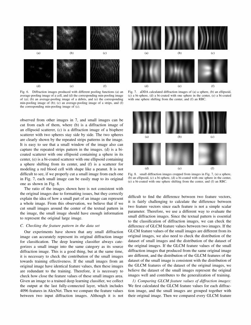
Program aDDA [19] is an open-source tool for simulatinglight scattering of particles using discrete dipole approximation(DDA) approach. aDDA can be used to calculate a diffractionimage of a scatterer. In theory, the diffraction image of ascatterer calculated from aDDA is identical to the p-DIFCacquired diffraction image of the same scatterer. We use aDDAsimulated diffraction images to check replication property oftextual patterns in the image to investigate whether partial ofthe image can represent the whole image. At the same time, weexpect each of the small image cuts from the original imageis unique. Fig. 7 shows 6 diffraction images calculated from 6different scatterers. Fig. 7a is a diffraction image of a spherescatterer, where the regular strips repeated in the image. If wecut a small window of image such as 300 × 300 pixels fromthe center of the original image (the size is 640× 480 pixels),the small image is sufficient to represent the textual pattern ofthe whole image.

If we shift the window from the center with small distance,we can cut more small images to represent the whole image,but each of the images is different. The same property can be

(a) (b) (c)

(d) (e) (f)

Fig. 6. Diffraction images produced with different pooling functions (a) anaverage-pooling image of a cell, and (d) the corresponding min-pooling imageof (a); (b) an average-pooling image of a debris, and (e) the correspondingmin-pooling image of (b); (c) an average-pooling image of a strips, and (f)the corresponding min-pooling image of (c).

observed from other images in 7, and small images can becut from each of them, where (b) is a diffraction image ofan ellipsoid scatterer, (c) is a diffraction image of a bispherescatterer with two spheres stay side by side. The two spheresare clearly shown by the repeated strips patterns in the image.It is easy to see that a small window of the image also cancapture the repeated strips pattern in the images. (d) is a bi-coated scatterer with one ellipsoid containing a sphere in itscenter, (e) is a bi-coated scatterer with one ellipsoid containinga sphere shifting from its center, and (f) is a scatterer formodeling a red blood cell with shape like a peanut. It is notdifficult to see, if we properly cut a small image from each onein Fig. 7, each small image can be easily map to its originalone as shown in Fig. 8.

The ratio of the images shown here is not consistent withthe original images due to formatting issues, but they correctlyexplain the idea of how a small part of an image can representa whole image. From this observation, we believe that if wecut small images around the center of the textual pattern inthe image, the small image should have enough informationto represent the original large image.

C. Checking the feature pattern in the data set

Our experiments have shown that any small diffractionimage can accurately represent its original diffraction imagefor classification. The deep learning classifier always cate-gorizes a small image into the same category as its sourcediffraction image. This is a good thing, but at the same time,it is necessary to check the contribution of the small imagestowards training effectiveness. If the small images from anoriginal image have identical feature values, then these imagesare redundant to the training. Therefore, it is necessary tocheck how close the feature values of these small images area.Given an image to a trained deep learning classifier, we collectthe output at the last fully-connected layer, which includes4096 features in AlexNet. Then we compare the feature valuesbetween two input diffraction images. Although it is not

(a) (b) (c)

(d) (e) (f)

Fig. 7. aDDA calculated diffraction images of (a) a sphere, (b) an ellipsoid,(c) a bi-sphere, (d) a bi-coated with one sphere in the center, (e) a bi-coatedwith one sphere shifting from the center, and (f) an RBC.

(a) (b) (c)

(d) (e) (f)

Fig. 8. small diffraction images cropped from images in Fig. 7, (a) a sphere,(b) an ellipsoid, (c) a bi-sphere, (d) a bi-coated with one sphere in the center,(e) a bi-coated with one sphere shifting from the center, and (f) an RBC.

difficult to find the difference between two feature vectors,it is fairly challenging to calculate the difference betweentwo feature vectors since each feature is not a simple scalarparameter. Therefore, we use a different way to evaluate thesmall diffraction images. Since the textual pattern is essentialto the classification of diffraction images, we can check thedifference of GLCM feature values between two images. If theGLCM feature values of the small images are different from itsoriginal images, we also need to check the distribution of thedataset of small images and the distribution of the dataset ofthe original images. If the GLCM feature values of the smalldiffraction images that produced from the same original imageare different, and the distribution of the GLCM features of thedataset of the small image is consistent with the distribution ofthe GLCM features of the dataset of the original images, webelieve the dataset of the small images represent the originalimages well and contributes to the generalization of training.

1) Comparing GLCM feature values of diffraction images:We first calculated the GLCM feature values for each diffrac-tion image, and the small images are grouped together withtheir original image. Then we compared every GLCM feature

Fig. 9. Compare the distribution of a GLCM feature values of the data setof the original images and the data set of the small images pooled from theoriginal images.

for all images in a group. If two images have different values ofat least one GLCM feature, the two images are considered asdifferent. Table V shows a partial comparison results of pooledsmall images and its original image in 6 GLCM features.Img − 1 to Img − 5 are pooled image from original imageImg−0. We checked every group of images, and did not findtwo identical images in each group.

2) Comparing GLCM feature distributions of datasets:We created a distribution of a GLCM feature for all originalimages that belong to the same type. Then we created the samedistribution for a group of small images that were producedfrom the original images. We compared the two distributionto see whether the distributions are consistent. Fig. 9 shows acomparison of the normal distribution of a GLCM feature ofthe original diffraction image data and the one of the smalldiffraction images pooled from the original ones.

We created a normal distribution with the normalized featurevalues (i.e. min-max normalization), mean of the values andstandard deviation, and the curve was drawn based on theprobability mass function. It is not difficult to see that thetwo distributions are not exactly the same. However, bothof them are normally distributed. Different GLCM featuresand different groups images are checked using the samedistribution. We found that the distribution pattens betweenthe dataset of original images and the datasets that are pooledor cropped images from the original images are consistent.Therefore, we conclude that both the pooling and croppingare effective for data augmentation of diffraction images.

V. RELATED WORK

Deep learning researchers are faced with the trade-offbetween using better deep learning architectures and bettertraining data [21]. However, building a deep learning archi-tecture for small training datasets is a grand challenge. Evena deep learning architecture is targeted for low-shot clas-sification requires data augmentation [22]. Therefore, usinglarge training data is a more feasible approach for building ahigh quality deep learning solution. For example, the originalAlexNet was trained with 1.2 million images, and the classifierfor categorizing the three categories of diffraction imagesrequired over 100,000 diffraction images for each category.However, many domain specific applications cannot produceenough data for the deep learning. Data augmentation throughproducing high quality artificial training data based on original

data is a widely adopted practice for enhancing the trainingdataset in deep learning.

Each domain specific application can produce artificial dataaccording to the domain models such as using aDDA forproducing diffraction images of cells. Sampling from a largeimage is also an effective approach for producing image data[23] [24]. In this paper, we have used cropping and poolingfrom original images for producing large volume of trainingdata. The augmented datasets are systematically evaluated interms of representativity, fidelity and variety.

Generative models are proposed recently for producingartificial data using deep learning techniques [25]. Althoughlarge amount of initial data are required to produce artificialdata using generative models, it is a promising technique forgenerating a large amount high quality artificial data. Throughlearning the transformation relation from similar datasets toproduce data for low-shot learning is also a promising ideafor data augmentation [22]. However, poor quality data couldcause serious problems such as wrong prediction or lowaccuracy of the classification.

Quality attributes of big data such as availability, usability,and reliability have been well defined in some publications[26] [7]. Although general techniques and tools are developedfor quality assurance of big data, much more work remains tobe done on the quality assurance of domain specific big datasuch as health care management data, social media data, andfinance data.

Machine learning algorithms such as Gradient BoostedDecision Tree (GBDT) are used for detecting data duplication[6]. Data filtering is an approach for quality assurance of bigdata through removing bad data from data sources. For exam-ple, Ekambaram et. al recently reported a machine learningapproach for finding label noise in the training data [27].

VI. SUMMARY AND FUTURE WORK

Training a deep learning model normally requires a largevolume of training data as well as high quality trainingdata. Large volume of training data may include noise data.Therefore, it is necessary to separate the noise data fromthe training data. In this paper, we proposed a deep learningapproach for the automated classification of training data intodifferent categories of data, one of which is a noise category.

In many cases, the original training data needs to betransformed to fit the input size requirements of deep learningmodels. In other cases, new data is required through dataaugmentation as the original data is insufficient in size. Wediscussed different data augmentation approaches. We havealso evaluated the quality of the training data through crossvalidation of the classification accuracy.

To demonstrate the proposed approaches to data aug-mentation and their effectiveness, we conducted a thoroughexperimental study on automated classification of massivediffraction images. The proposed approaches and experiencecollected from this experimental study can be adopted for dataaugmentation and evaluation of big data in other domains.

TABLE VA COMPARISON OF GLCM FEATURE VALUES AMONG DIFFRACTION IMAGES

ASM CON COR VAR IDM SAVImg-1 0.069028397 0.300829789 0.978817148 0.164436833 0.597584362 0.231334924Img-2 0.656232866 0.224157652 0.980417054 0.130393754 0.864684597 0.109085359Img-3 0.967753732 0.017326016 0.688163634 0.000792628 0.989551474 0.026260393Img-4 0.026913115 0.159871456 0.99144913 0.166720538 0.621992081 0.292738468Img-5 0.587408623 0.235948351 0.951577511 0.063657455 0.836049419 0.093207132Img-0 0.329891354 0.001331282 0.997723423 0.117280715 0.84966343 0.282349741

ACKNOWLEDGMENT

The authors would like to thank Dr. Xin-Hua Hu andPruthvish Patel at East Carolina University for assistancewith the experiments. This research is supported in part bygrants #1560037 and #1730568 from the National ScienceFoundation. We gratefully acknowledge NVIDIA Corporationfor Tesla K40 GPU gift, which is used for conducting thisresearch.

REFERENCES

[1] Y. Bengio, “Learning deep architectures for ai,” Foundations and Trendsin Machine Learning, vol. 2, no. 1, pp. 1–127, 2009.

[2] E. Giannoulatou, S.-H. Park, D. Humphreys, and J. Ho, “Verificationand validation of bioinformatics software without a gold standard: a casestudy of bwa and bowtie,” BMC Bioinformatics, vol. 15(Suppl 16):S15,2014.

[3] J. Zhang, Y. Feng, M. S. Moran, J. Lu, L. Yang et al., “Analysis ofcellular objects through diffraction images acquired by flow cytometry,”Opt. Express, vol. 21, no. 21, pp. 24 819–24 828, 2013.

[4] J. A. Saez, B. Krawczyk, and M. Wozniak, “On the influence of classnoise in medical data classification: Treatment using noise filteringmethods,” Applied Artificial Intelligence, vol. 30, no. 6, pp. 590–609,Jul. 2016.

[5] J. Gao, C. Xie, and C. Tao, “Big data validation and quality assurance– issuses, challenges, and needs,” in 2016 IEEE Symposium on Service-Oriented System Engineering (SOSE), March 2016, pp. 433–441.

[6] C. H. Wu and Y. Song, “Robust and distributed web-scale near-dupdocument conflation in microsoft academic service,” in 2015 IEEEInternational Conference on Big Data (Big Data), Oct. 2015, pp. 2606–2611.

[7] V. Gudivada, R. Raeza-Yates, and V. Raghavan, “Big data: Promises andproblems,” IEEE Computer, vol. 48, no. 3, pp. 20–23, 2015.

[8] K. Jacobs, J. Lu, and X. Hu, “Development of a diffraction imagingflow cytometer,” Opt. Lett., vol. 34, no. 19, p. 29852987, 2009.

[9] A. Krizhevsky, I. Sutskever, and G. E. Hinton, “Imagenet classifica-tion with deep convolutional neural networks,” in Advances in neuralinformation processing systems, F. Pereira, C. Burges, L. Bottou, andK. Weinberger, Eds., 2012, pp. 1097–1105.

[10] C. J. Burges, “A tutorial on support vector machines for pattern recog-nition,” Data Mining and Knowledge Discovery, vol. 2, pp. 121–167,Jan. 1998.

[11] J. Ding, D. Zhang, and X. Hu, “An application of metamorphic testingfor testing scientific software,” in 1st Intl. workshop on metamorphictesting with ICSE, Austin, TX, May 2016.

[12] K. Dong, Y. Feng, K. Jacobs, J. Lu, R. Brock et al., “Label-freeclassification of cultured cells through diffraction imaging,” Biomed.Opt. Express, vol. 2, no. 6, p. 17171726, 2011.

[13] C.-C. Chang and C.-J. Lin, “LIBSVM: A library for support vectormachines,” ACM Transactions on Intelligent Systems and Technology,vol. 2, pp. 27:1–27:27, 2011.

[14] R. Haralick, “On a texture-context feature extraction algorithm forremotely sensed imagery,” in Proceedings of the IEEE Computer SocietyConference on Decision and Control, Gainesville, FL, Dec. 1971, pp.650–657.

[15] S. K. Thati, J. Ding, D. Zhang, and X. Hu, “Feature selection and anal-ysis of diffraction images,” in 4th IEEE Intl. Workshop on InformationAssurance, Vancouver, Canada, August 2015.

[16] J. Ding, J. Wang, X. Kang, and X. Hu, “Building an svm classifier forautomated selection of big data,” in 2017 IEEE International Congresson Big Data, Honolulu, HI, 2017.

[17] S. Vilkomir, J. Wang, N. L. Thai, and J. Ding, “Combinatorial methodsof feature selection for cell image classification,” in 2017 IEEE Intl.Workshop. on Combinatorial Testing and Applications, Prague, Czech,July 2017.

[18] J. Ding, X. Kang, X. H. Hu, and V. Gudivada, “Building a deep learningclassifier for enhancing a biomedical big data service,” in 2017 IEEEIntl. Conf. on Services Computing, Honolulu, HI, June 2017.

[19] (2016, Sept.) Adda project. [Online]. Available: https://github.com/adda-team/adda

[20] (2017, Jan.) Deep learning tutorial. [Online]. Available:http://deeplearning.net/tutorial/lenet.html

[21] H.-C. Shin, H. R. Roth, M. Gao, L. Lu, Z. Xu, I. Nogues, J. Yao,D. Mollura, and R. M. Summers, “Deep convolutional neural networksfor computer-aided detection: Cnn architectures, dataset characteristicsand transfer learning,” IEEE transactions on medical imaging, vol. 35,no. 5, pp. 1285–1298, 2016.

[22] B. Hariharan and R. B. Girshick, “Low-shot visual objectrecognition,” CoRR, vol. abs/1606.02819, 2016. [Online]. Available:http://arxiv.org/abs/1606.02819

[23] D. Ciresan, A. Giusti, L. M. Gambardella, and J. Schmidhuber, “Mitosisdetection in breast cancer histology images with deep neural networks,”in Intl. Conf. on Medical Image Computing and Computer-assistedIntervention, 2013, pp. 411–418.

[24] B. Dong, L. Shao, M. D. Costa, O. Bandmann, and A. F. Frangi, “Deeplearning for automatic cell detection in wide-field microscopy zebrafishimages,” in 2015 IEEE 12th Intl. Symposium on Biomedical Imaging(ISBI), April 2015, pp. 772–776.

[25] (2017, Jan.) Open ai: Generative models. [Online]. Available:https://openai.com/blog/generative-models/

[26] L. Cai and Y. Zhu, “The challenges of data quality and data qualityassessment in the big data era,” Data Science Journal, vol. 14:2, pp.1–10, 2015.

[27] R. Ekambaram, D. Goldgof, and L. Hall, “Finding label noise examplesin large scale datasets,” in 2017 IEEE Intl. Conf. on Systems, Man, andCybernetics (SMC), Banff, Canada, Oct. 2017.