BACKGROUND CONCENTRATION DATA

Technical Support Document

NOVEMBER 16, 2015 IOWA DEPARTMENT OF NATURAL RESOURCES

Alyssa Fizel

1

Table of Contents Summary ............................................................................................................ 2

Default Background Concentrations .................................................................... 2

Establishing NO2 Urban & Rural Delineation using CAMx....................................................................... 3

Time-varying PM2.5 Background Concentrations .................................................................................... 6

Proposing Alternative Background Concentrations ............................................. 8

2012-2014 Site-Specific Monitor Data ..................................................................................................... 9

Statewide Default Ozone Background Data ...................................................... 13

2

Summary Background concentrations represent natural sources, non-industrial human activity, and distant industrial facilities. The background concentrations are added to dispersion modeling results for comparison to the National Ambient Air Quality Standards (NAAQS). This technical support document contains information supporting the new default background concentrations, the new background ozone data to be used in a Tier 3 NO2 analysis and addressing the use of alternative backgrounds. The background data should be used in conjunction with the 2010-2014 meteorological data.

Default Background Concentrations The Iowa Department of Natural Resources (DNR) provides default background concentrations that can be used without prior approval in dispersion modeling analyses. The default background concentrations have been re-evaluated with 2012-2014 ambient air monitoring data. Table 1 summarizes the default background concentrations for all criteria pollutants. The background concentrations have been calculated using the upper limit of the 95% confidence interval of the design concentrations at all non-source-oriented monitors across the state. Calculating the default concentrations in this way ensures that they will be conservatively representative of the entire state.

Table 1. Summary of Default Background Concentrations

Pollutant Averaging Period Background Concentrations (μg/m3)

NO2 1-Hour Urban: 84; Rural: 18* Annual Urban: 15; Rural: 4*

SO2

1-Hour 7* 3-Hour 7*

24-Hour 3* Annual 1*

PM2.5 24-Hour 23 (Winter: 23; Spring: 20; Summer: 20; Fall: 20) Annual 9.8

PM10 24-Hour 52

CO 1-Hour 3,500 8-hour 2,100

Pb 3-Month Rolling Average 0 *Only one monitor, this is the design value not the 95% confidence limit

There are two major changes from the last set of default background concentrations. The first is that the state is no longer delineated into east and west regions for PM2.5. The PM2.5 design concentrations were not significantly different between the east and west regions of the state, negating the need for separate background concentrations. Please refer to Figures 5 & 6 for the specific design values at each monitor. The previously delineated west region contained the Council Bluffs, Emmetsburg, Lake Sugema, Sioux City and Viking Lake monitors. The remaining monitors were previously delineated to the east region.

The second major change is in regard to the SO2 default background concentrations. Per the 2011 National Emissions Inventory (NEI) almost all SO2 emissions in Iowa (>97%) come from industrial activities, and 95% are from coal combustion. There are a relatively small number of industrialized areas contributing to this majority of statewide emissions, but over half of the existing SO2 monitors in Iowa are located near these areas. Including these monitors in the calculation of the default background would result in an overly conservative background for the majority of the state. For these reasons the DNR has determined that it is appropriate to use a background

3

concentration that is more representative of natural background levels and to explicitly model nearby SO2-emitting facilities. The default SO2 background concentrations summarized herein are the design values at the Lake Sugema monitor. This monitor is located in a rural area that is not influenced by industrial activity. Nearby sources will be determined on a case-by-case basis. Contact the Iowa Department of Natural Resources at (515) 725-8200 and ask for a member of the dispersion modeling team to obtain information on nearby SO2 sources.

Establishing NO2 Urban & Rural Delineation using CAMx PURPOSE Modeled NO2 concentrations produced by the Comprehensive Air Quality Model with Extensions (CAMx) model were used to identify an appropriate geographical delineation between urban and rural background concentrations. The modeled NO2 concentrations were produced from an annual simulation covering the year 2011.

MODEL INPUTS CAMx is an Eulerian photochemical dispersion model that allows for integrated "one-atmosphere" assessments of gaseous and particulate air pollution over many scales ranging from sub-urban to continental. The CAMx modeling domain covered the entire continental U.S., but emphasis was placed on grid cells over Iowa. The resolution of the domain was 12 km, which is much finer than the ambient air observation network. The annual simulation used model-ready emissions data from EPA’s 2011 modeling platform. Meteorological inputs were incorporated from an annual 2011 simulation evaluated by the DNR and conducted by the EPA using the Weather Research and Forecasting (WRF) meteorological model.

METHODOLOGY The urban and rural areas were delineated using predicted NO2 concentration gradients from CAMx. There are two monitors located in urban areas: Des Moines and Davenport (see Figures 3 & 4). Both monitors are located within the urban area but far enough away from major industry to provide an accurate representation of an urban background concentration. There is one monitor location in a rural area: Lake Sugema (see Figures 3 & 4). This monitor is an accurate representation of a rural background concentration.

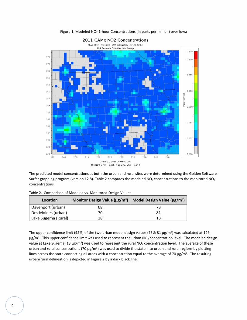
The concentrations generated from CAMx data were processed at each grid cell to produce the total NO2 concentrations for the 1-hour NO2 standard. The data represented the predicted 98th percentile daily maximum 1-hour concentrations from CAMx. The 1-hour concentrations were chosen instead of the annual concentrations because the purpose of this analysis was to define the gradients between urban and rural areas of the state. The short-term concentrations provide a more appropriate metric for depicting the localized influences. Figure 1 shows the final analyzed NO2 concentration field.

4

Figure 1. Modeled NO2 1-hour Concentrations (in parts per million) over Iowa

The predicted model concentrations at both the urban and rural sites were determined using the Golden Software Surfer graphing program (version 12.8). Table 2 compares the modeled NO2 concentrations to the monitored NO2

concentrations.

Table 2. Comparison of Modeled vs. Monitored Design Values

Location Monitor Design Value (μg/m3) Model Design Value (μg/m3)

Davenport (urban) 68 73 Des Moines (urban) 70 81 Lake Sugema (Rural) 18 13

The upper confidence limit (95%) of the two urban model design values (73 & 81 μg/m3) was calculated at 126 μg/m3. This upper confidence limit was used to represent the urban NO2 concentration level. The modeled design value at Lake Sugema (13 μg/m3) was used to represent the rural NO2 concentration level. The average of these urban and rural concentrations (70 μg/m3) was used to divide the state into urban and rural regions by plotting lines across the state connecting all areas with a concentration equal to the average of 70 μg/m3. The resulting urban/rural delineation is depicted in Figure 2 by a dark black line.

5

Figure 2. Urban/Rural Delineation (black line = 70 μg/m3)

DEFAULT NO2 BACKGROUND CONCENTRATIONS BY COUNTY In order to simplify the implementation of the default background concentrations it was decided to limit the extent of the areas represented by the urban background to the county in which the urban influence originates. The default urban background counties are:

• Polk • Pottawattamie • Scott

For all three locations the urban influence does not extend over the entire county in which it originated. In cases where a project occurs in a default urban background county, the Department will consider a rural background if the location can be shown to be outside the urban influence area in the data. A Google Earth KML file is provided on the website so that applicants can zoom in to a specific area to make this determination. All other counties are considered rural even if the black line partially crosses into the county.

6

Time-varying PM2.5 Background Concentrations The Iowa DNR previously provided daily background concentrations to supplement the default fine particulate matter (PM2.5) background concentrations for the state of Iowa. The daily background concentrations were to be paired with model predictions to aid in showing modeled attainment of the National Ambient Air Quality Standards (NAAQS) for expansion and new construction. This practice – known as paired-sums – was intended to account for the day-to-day variability of the background concentrations. Due to the spatial and temporal variability on an hourly basis as well as limitations in hourly ambient monitoring observations, the EPA has since released guidance indicating that the paired-sums approach is not appropriate. However, EPA recognizes that demonstrating compliance with the PM2.5 NAAQS can be difficult without considering the temporal variability in background concentrations. For this reason EPA included a seasonal time-varying background approach in their Guidance for PM2.5 Permit Modeling (May 20, 2014). Using this guidance will also allow for the use of time-varying background concentrations in PSD projects.

The use of these seasonal background concentrations should be acceptable in most cases. However, per section 2.5 of the addendum to the User’s Guide for the AMS/EPA Regulatory Model – AERMOD, the presence of calm winds can cause an under-estimate of any background concentration that is input into the model. This will be evaluated on a case-by-case basis, and if it is found that the background contribution is under-estimated the analysis may need to be reevaluated. SEASONAL BACKGROUND CONCENTRATIONS The seasonal background data was based on a three year period (Jan. 2012-Dec. 2014). In order to have the monitored data, provided by calendar year, correspond to the seasonal periods (Winter = Dec – Feb, Spring = Mar – May, Summer = Jun – Aug, Autumn = Sep – Nov), data from December 2014 is used for December of Q1 (ordinarily Dec 2011).

The procedure to determine the four seasonal background concentrations to be used in AERMOD for a PM2.5 analysis followed the EPA’s PM2.5 modeling guidance (referenced above) under Section IV.3 and Appendix E. The monitored data for cities that have multiple monitors was averaged together first (Cedar Rapids, Clinton, Davenport, Des Moines, Muscatine, Sioux City and Waterloo) and then the EPA procedure referenced above was used to determine the seasonal background concentrations for each of these sites as well as the stand-alone sites in Backbone State Park, Council Bluffs, Emmetsburg, Iowa City, Keokuk, Keosauqua and Viking Lake State Park. Table 3 summarizes the site-specific seasonal concentrations for all 14 sites.

7

Table 3. Seasonal PM2.5 24-hr Site-Specific Background Concentrations

City/Site Concentration (μg/m3) Winter Spring Summer Autumn

Backbone State Park 20 19 19 20 Cedar Rapids 23 21 20 20

Clinton 24 21 19 20 Council Bluffs 25 19 19 19

Davenport 24 21 20 21 Des Moines 21 20 20 20 Emmetsburg 20 19 18 17

Iowa City 23 21 19 19 Keokuk 25 21 21 21

Lake Sugema 21 16 17 17 Muscatine 23 21 18 22 Sioux City 22 18 20 19

Viking Lake State Park 18 17 19 17 Waterloo 20 17 18 19

The 95% confidence limit was then determined for each of the seasons from the seasonal background concentrations of these 14 sites. The background concentrations for the PM2.5 24-hour averaging period are as follows:

Table 4. Seasonal PM2.5 24-hr Background Concentrations

Season Concentration (µg/m3)

Winter 23 Spring 20

Summer 20 Fall 20

8

Proposing Alternative Background Concentrations The values listed in Table 1 are the default background concentrations for any location in the state of Iowa. However, the default background concentrations are conservative by design, allowing applicants to use them without prior approval or additional justification. In some cases an applicant may wish to propose a background concentration from site specific monitoring data that is more representative of their location.

The use of any alternative background concentration will require prior approval by the DNR. There are no specific criteria required for approval, and the information needed to adequately justify an alternate background will vary from case to case. The justification should be a well-reasoned weight-of-evidence approach that supports the chosen background concentration(s). The following are examples of the type of information that could be used to support an alternative background concentration:

• Monitor location • Source of data • Proximity of chosen monitor to other sources of the applicable pollutant(s) • Proximity of the facility in question to other sources of the applicable pollutant(s) (excluding any sources

being explicitly modeled) • Quantity of emissions of the applicable pollutant(s) in the vicinity of the chosen monitor • Quantity of emissions of the applicable pollutant(s) in the vicinity of the facility in question (excluding any

sources being explicitly modeled) • Land use & topography • Prevailing wind direction & local meteorology

There is no required screening distance when evaluating information from sources “in the vicinity”. However, a radius of 10 km to county-wide are appropriate distances. The “significant concentration gradient” concept referenced by EPA in Appendix W would also be an appropriate method of determining a screening distance. In the event that specific guidance related to “significant concentration gradients” becomes available it should be used for this purpose. The following sources may be helpful in developing justification for an alternative background:

• Iowa DNR Facility Explorer • Operating Permits • Ambient Air Monitoring Data

9

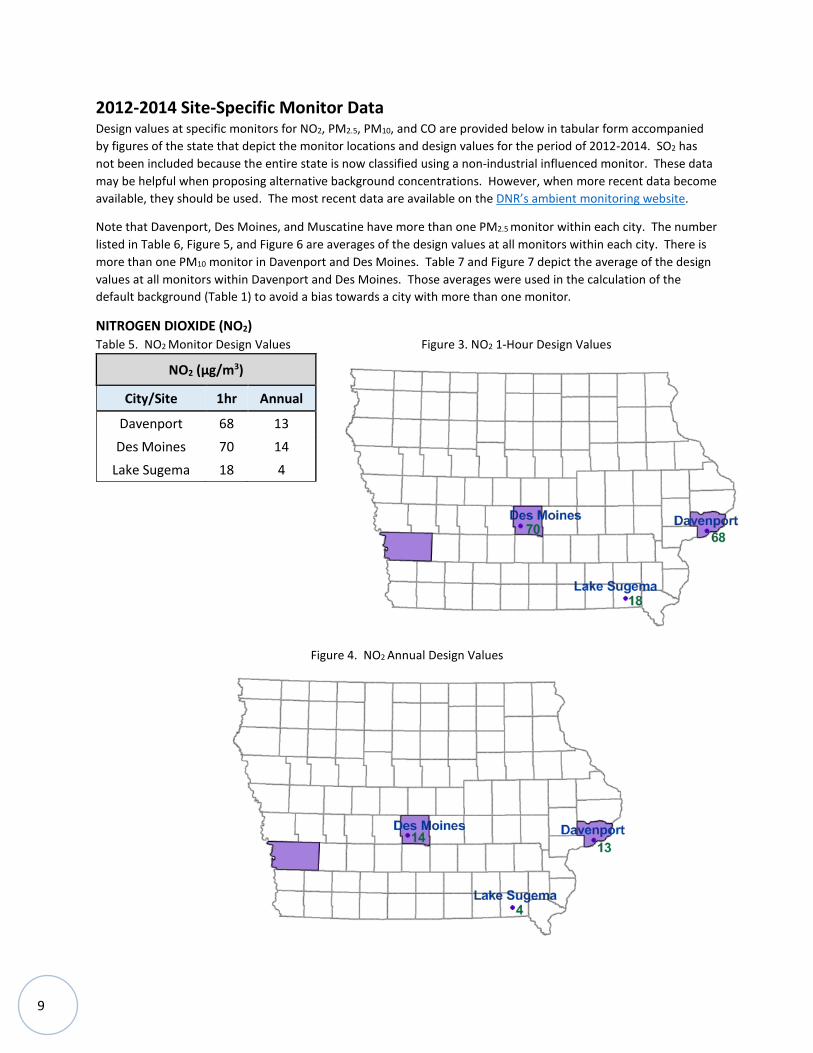
2012-2014 Site-Specific Monitor Data Design values at specific monitors for NO2, PM2.5, PM10, and CO are provided below in tabular form accompanied by figures of the state that depict the monitor locations and design values for the period of 2012-2014. SO2 has not been included because the entire state is now classified using a non-industrial influenced monitor. These data may be helpful when proposing alternative background concentrations. However, when more recent data become available, they should be used. The most recent data are available on the DNR’s ambient monitoring website.

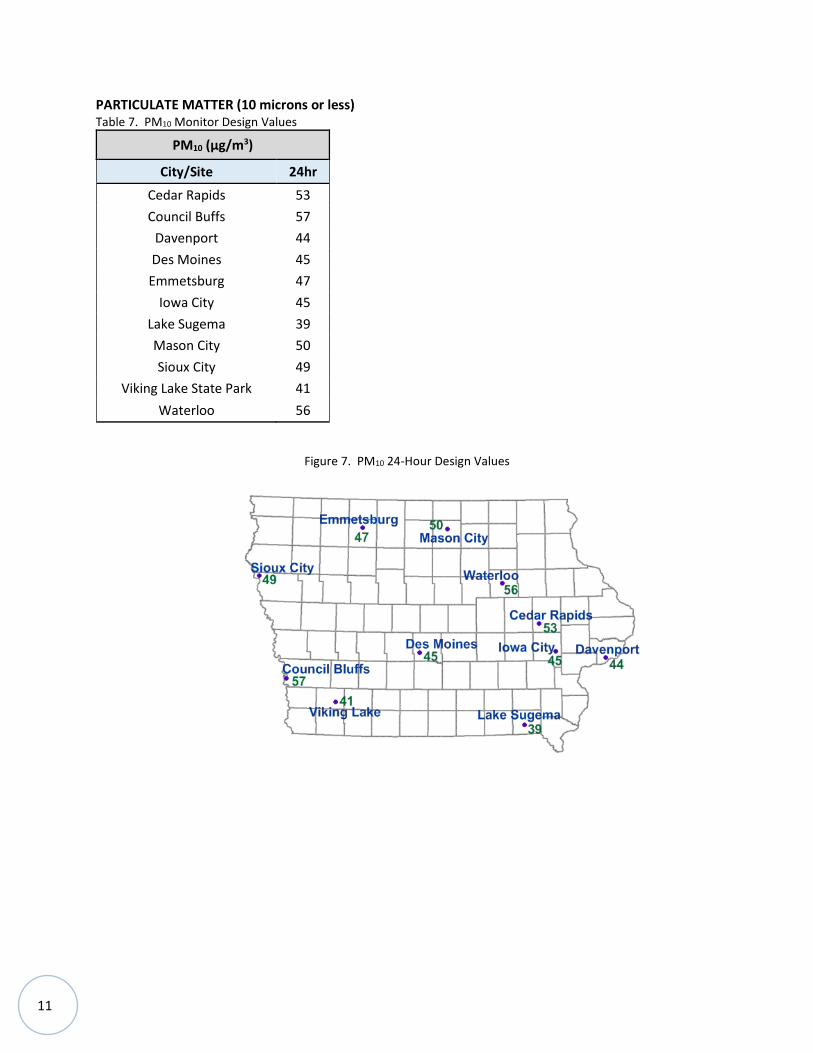
Note that Davenport, Des Moines, and Muscatine have more than one PM2.5 monitor within each city. The number listed in Table 6, Figure 5, and Figure 6 are averages of the design values at all monitors within each city. There is more than one PM10 monitor in Davenport and Des Moines. Table 7 and Figure 7 depict the average of the design values at all monitors within Davenport and Des Moines. Those averages were used in the calculation of the default background (Table 1) to avoid a bias towards a city with more than one monitor.

NITROGEN DIOXIDE (NO2) Table 5. NO2 Monitor Design Values Figure 3. NO2 1-Hour Design Values

NO2 (μg/m3)

City/Site 1hr Annual

Davenport 68 13 Des Moines 70 14

Lake Sugema 18 4

Figure 4. NO2 Annual Design Values

10

PARTICULATE MATTER (2.5 microns or less) Table 6. PM2.5 Monitor Design Values Figure 5. PM2.5 24-Hour Design Values

PM2.5 (μg/m3)

City/State 24hr Annual Backbone State Park 21 9.0

Cedar Rapids 23 9.5 Clinton 23 9.5

Council Bluffs 24 9.8 Davenport 24 10.0

Des Moines 21 8.9 Emmetsburg 21 8.2

Iowa City 22 9.2 Keokuk 24 10.8

Lake Sugema 20 8.4 Muscatine 24 10.1 Sioux City 24 9.1

Viking Lake State Park 20 8.3 Waterloo 21 9.5

Figure 6. PM2.5 Annual Design Values

11

PARTICULATE MATTER (10 microns or less) Table 7. PM10 Monitor Design Values

PM10 (μg/m3)

City/Site 24hr

Cedar Rapids 53 Council Buffs 57

Davenport 44 Des Moines 45 Emmetsburg 47

Iowa City 45 Lake Sugema 39 Mason City 50 Sioux City 49

Viking Lake State Park 41 Waterloo 56

Figure 7. PM10 24-Hour Design Values

12

CARBON MONOXIDE (CO) Table 8. CO Design Monitor Values

CO (μg/m3)

City/Site 1hr 8hr

Cedar Rapids 2514 1504 Davenport 1290 803

Des Moines 1979 1267

Figure 8. CO 1-hour Design Values

Figure 9. CO 8-Hour Design Values

13

Statewide Default Ozone Background Data In 2013, an ozone data sensitivity analysis was conducted by the DNR which concluded that the spatial variation of ozone concentrations observed across Iowa did not significantly affect the NO2 concentrations predicted by AERMOD. This conclusion supported making a statewide ozone background file.

The ozone data is intended for use in the 1-hour NO2 modeling analyses when the non-regulatory default Tier 3 Ozone Limiting Method (OLM) or Plume Volume Molar Ration Method (PVMRM) is utilized in AERMOD. Prior approval for use of either OLM or PVMRM is required. OLM and PVMRM are screening methods used to estimate the conversion of NO to NO2.

The DNR has generated a background ozone concentration file for use anywhere in the state for the time period coinciding with the 2010-2014 meteorological dataset. Please note that the data is in ppb.

The file provided above is an average of the ozone monitor data collected from 16 sites across the state. Note that two of the sixteen locations have two ozone monitors within the same area. Both monitors within the same area were averaged first, before averaging across all sites. This was done to avoid a bias towards a site with more than one monitor. Over the five years of data (2010-2014), there were 58 hours missing, with the largest gap being only three hours. Linear interpolation was used to fill all missing data.

COMPARISON OF 2010-2014 OZONE DATA TO 2005-2009 OZONE DATA Figure 10 depicts the histograms for each ozone data set. The data sets have a very similar distribution, and the average of the 2010-2014 data set (28 ppb) is only slightly higher than the 2005-2009 data set (26 ppb). This supports the continued use of a statewide ozone data set.

Figure 10. Histograms of Old and New Ozone Data