BANCO DE PORTUGAL

Economic Research Department

ANALYSIS OF DELINQUENT FIRMS USING

MULTI-STATE TRANSITIONS

António R. Antunes

WP 5-05 June 2005

The analyses, opinions and findings of these papers represent the views of the

authors, they are not necessarily those of the Banco de Portugal.

Please address correspondence to António R. Antunes Economic Research Department,

Banco de Portugal, Av. Almirante Reis no. 71, 1150-012 Lisboa, Portugal;

Tel: 351–21–3128246 Fax: 351–21–3107806; email: aantunes@bportugal.pt.

Analysis of delinquent firms using multi-state

transitions∗

Antonio R. Antunes†

Banco de Portugal and Universidade NOVA de Lisboa

Mars 18, 2005

Abstract

This paper analyzes the behavior of firms with defaulted credits in terms of

recovery or extinction. By defining classes for the severity of default, survival models

for the multiple transitions from each class are estimated. The models are used to

simulate the evolution of a firm’s credit conditional on its characteristics. Estimates

for the expected recovery or extinction rates are constructed from these simulations.

They show that (i) the severity of default strongly influences the probability of

extinction; (ii) for less severe default episodes, recovery is faster than extinction,

and the opposite is true for more severe defaults; (iii) larger firms tend to display

better outcomes; (iv) and the number of employees is the single most important

determinant of the time profile of the extinction/recovery process. Estimates of a

loss given default measure suggest that the supervision recommendations found in

the literature are appropriate.

Keywords: credit default, survival analysis, firms

JEL: C15, C41, G28, G33

∗I thank the contributions of my colleagues at the Banco de Portugal research department, especiallyMaria Clara Soares, Nuno Martins, Nuno Ribeiro and Pedro Portugal.

†Email: aantunes@bportugal.pt. Address: Av. Almirante Reis, 71, 6o, 1150-012 Lisboa, Portugal.

1

1 Introduction

The assessment of credit risk taking by financial intermediaries evolved rapidly over the

last two decades. The continuous improvement in the capacity to process information

permitted major qualitative steps in the late 1990’s. An example is the estimation of the

ex ante propensity of firms to default, which became an alternative to the passive wait

for the material observation of the default of each particular borrower.

The New Basel Accord (Basel II) set out by the Basel Committee on Banking Super-

vision (2004) incorporates the ex ante nature of credit risk, while requiring an interaction

between capital adequacy rules and provisioning requirements. Specific provision require-

ments remain very diverse across countries and in most jurisdictions are likely not to

coincide with the notion of “impairment adjustment” as set out in the IAS/IFRS.

Using information on credit for non-financial firms, as well as information concerning

the type of firm, this paper proposes a method for measuring the long-run propensity of

companies to remain in default, once it was objectively observed, or to evolve either to

recovery or to definitive delinquency.

Beyond more sophisticated measures of loan losses, the model allows for the estimation

of recovery and/or loss given default rates. Both measures are relevant for impairment

assessment under IAS, calibration of provisioning rules, and capital adequacy assessment

under the advanced version of the Basel II Internal Ratings-Based (IRB) method.

Due to the inherently private nature of credit exposures, there is not much published

work with precise estimates of measures such as the probability of extinction or recovery

of firms once a default episode has been recorded. The Internal Ratings-Based approach

of the Basel Accord for banking supervision uses precisely this concept when defining loss

given default (LGD) as the expected loss on a specific loan once default has occurred.

The Basel Committee on Banking Supervision (2001) outlines different LGD calculation

methods for a large array of exposures. The existence of collateral is explicitly acknowl-

edged as an important mitigating factor on LGD estimates. Other factors include the

type of exposure (corporate, retail, financial institutions) and maturity of loans, for in-

stance. In the context of financial supervision, LGD may be calculated using the lender’s

2

internal methods (the “advanced” approach of the IRB method), or taken off-the-shelf for

the purpose at hand (the “foundation” approach). In this case, the recommended value

for the most common exposures is 50 percent. In our case, probabilities are calculated

conditional on the state of the loan and other variables that characterize the firm. To

obtain an LGD comparable to the values found in the supervision literature, we have to

integrate across state distributions of the first occurrence of default, conditional on the

firms’ characteristics.

Beyond long-run measures such as the one reported by the Basel Committee on Bank-

ing Supervision, little is known about the time pattern of extinction and recovery of the

firms. For instance, given that a firm is going to become extinct, when is that going to

happen? Does recovery occur faster than extinction or is it the other way around? The

answers to these and other questions are important in that they allow for a proper justi-

fication of the postponement or anticipation of specific provisions, for instance, and also

because they allow a proper monitoring of the evolution of firms with a default record. If,

for instance, we know that a particular type of firm typically becomes extinct relatively

fast and recovers relatively slowly, one could view a long survival time as an indication

that the firm is going to survive with a high probability. To answer this kind of questions,

duration analysis presents obvious advantages over other possible approaches to this type

of problem, such as probit estimates.

We use duration analysis with competing risks to assess the survival of firms in a

given state. States are defined primarily in terms of the severity of the credit default

episode. This is measured as the ratio between the amount of on-sheet overdue credit

of a firm, and the total amount of on-sheet outstanding credit. Based on estimates of

proportional hazard models for each state (where each competing risk is the transition to

failure, recovery, or another state), implied probabilities for a semi-Markov process are

calculated. We then simulate trajectories of credit history for a large number of firms and

estimate probabilities of extinction and recovery conditional on the length of the observed

credit episode and other characteristics of the firms. Standard errors for these estimates

are calculated by performing multiple experiments, where the semi-Markov transition

3

probabilities are calculated from realizations of the parameter vector that respect the

distribution of the proportional hazard models estimated parameters.

The data come from two sources, the Central de Responsabilidades de Credito (CRC)

database, and an internal comprehensive database used for statistical purposes at Banco

de Portugal. The CRC comprises monthly credit information on non financial, private

firms reported to the Portuguese central bank. Reporting is mandatory. Only firms that

have had a non-repayment episode are considered in the analysis. The internal statistical

purpose database has yearly information on the firm’s number of employees, sales, activity

sector, and region. Both databases virtually represent the respective universe and their

intersection spans the period from January 1995 to December 2000. In order to avoid

misreported or absent data from the CRC, we use end-of-the-period, quarterly data.

The estimation and simulation procedures enable us to compute probabilities and

other quantitative measures of the firms’ recovery or extinction processes. We assess the

severity of default using the ratio of due credit to total outstanding credit. We shall

call this measure the “default ratio”. The first broad conclusion is that the severity

of default strongly and significantly influences the probability of extinction. For the

least severe default episodes (the ones with a default ratio between 10 and 25 percent),

recovery is faster than extinction, and the opposite is true for more severe cases. The

simulations also suggest that larger firms tend to display better outcomes, and that the

number of employees is the single most important determinant of the time profile of the

extinction/recovery process. Estimates of a loss given default measure suggest that the

supervision recommendations found in the literature are appropriate.

The characterization of deliquescent firms presented in this paper suffers from several

shortcomings. The first is that credit data specific to each firm is aggregated across

financial institutions. It is therefore impossible to distinguish between different loans of

the same firm. This is unfortunate because loss given default estimates for supervisory

purposes should, in principle, distinguish between types of credit and maturity. Moreover,

the existence of collateral is not reported.

As for the estimation and the simulation strategies used, it is clear that the hypothesis

4

of independence between the firm’s history in the state space prior to entry in current

state, and its duration of stay in the current state, merits some thoughts. However, the fact

that we used four intermediate states mitigates this concern, as dependence across spells

in different states is likely to be smaller if states are not too dissimilar. If, for instance,

we defined a continuum of states, then we would end up with a perfect description of the

underlying statistical process, should one exist.

The rest of the paper is organized as follows. Section 2 describes the estimation and

simulation strategies. Section 3 describes the data used for estimation purposes. Section

4 presents the empirical results, and section 5 concludes.

2 Modelling transitions

2.1 Definition of states

Based primarily on the severity of the credit default episode r for a given firm in a known

moment, we define J states. The severity of the credit episode is calculated as the ratio

of on-sheet overdue credit, x, to the total amount of outstanding credit d.

There are two absorbing states in our analysis. A state is absorbing if a firm stays there

forever once it enters that state. The two states correspond to extinction and recovery.

A firm is defined as extinct if r exceeds 90 percent and the amount of overdue credit is

higher than 100 euros. Recovery occurs whenever r is lower than 10 percent or d is smaller

than 100 euros. Sensitivity analysis for these thresholds will be provided in appendix A.

We define four non absorbing states. Provided d is higher than 100 euros, we use

thresholds for r of 25, 50 and 75 percent. Table 1 summarizes the definitions of states.

The motivation for definition of extinction comes from the fact that firms often stay in

a database such as the CRC long after they became effectively bankrupt, or at least in a

situation where claims on outstanding debt are already fully provisioned. An alternative

criterion for firm extinction would lie, for instance, in the use of databases with information

on firms that were declared to have ended legal activity. This kind of database exists in

many countries. In the Portuguese case, however, the information is updated at a much

5

lower frequency than the CRC, and often with a considerable lag.

It is worth noting that the fact that recovery is an absorbing state in the statistical

analysis does not imply that, for instance, a real world firm recovering from a bad credit

episode will never default again. We assume that once a firm recovers, the probability

that it again enters the pool of financially stressed firms is statistically not different from

that of any other firm with the same characteristics.

The fact that many firms simply disappear from the CRC database, and therefore

cannot be labelled as “extinct” or “recovered”, means in practical terms that these obser-

vations are censored. The mere observation that they were present in the CRC for some

period is taken into account in the parameter estimation, even though the destination

state is not observed.

Another observation is that different definitions of recovery or extinction could have

been used in this analysis. For instance, one might have considered that a firm was

basically bankrupt from the moment when some bank wrote off its liabilities. This may

be seen as an indication of definitive non-recoverability of overdue claims. However, the

correlation between an indicator of the existence of write-offs above the 100 euros and

the first occurrence of the recovery state is only -8.5 percent. (The correlation with the

indicator of extinction is the same but positive.) This amounts to saying that many firms

that essentially have a small amount of overdue credit experience write-offs.

The assumption that extinction is absorbing is acceptable because it implies that the

extinction probability calculated in this paper is an upper bound for its real counterpart.

As for the recovery rate, its definition is sufficiently conservative to make sure that no

significant impact on the bank’s balance sheet occurs for a threshold lower than 10 percent.

See appendix A for more details on this.

The thresholds chosen for r are motivated by the accounting rules of many countries,

which establish different provisioning procedures based on r being less (or more) than 25

percent, 50 percent, or 75 percent.

6

State number State label Conditioning event1 “Recovery” r ≤ 0.1 or x ≤ 1002 “Extinction” r ≥ 0.9 and x > 1003 0.1 < r < 0.25 and x > 1004 0.25 ≤ r < 0.5 and x > 1005 0.5 ≤ r < 0.75 and x > 1006 0.75 ≤ r < 0.9 and x > 100

Table 1: Definition of states. Amount of defaulted credit x in euros, r in natural units.

2.2 Duration models

We assume that the current state and the firm’s vector of characteristics, as well as the

duration of the firm’s stay in that state, determine the probability of transition to another

state per unit of time. For expositional purposes, suppose for now that there are only

two states, the origin and the destination states, and that all firms are equal. Define

T as the random variable describing the moment when the transition occurs. Assuming

that the firm enters the origin state at time 0, T is the duration of the firm’s stay in

the origin state. Define P (t ≤ T < t + dt|T ≥ t) as the probability that a transition to

the destination state occurs between instants t and t + dt, given that the firm survived

in the origin state up to moment t. The hazard function associated with the probability

measure P is defined as

h(t) = limdt→0

P (t ≤ T < t + dt|T ≥ t)

dt.

If there is a large number of firms, h(t) is, among all the firms that have not transited to

the destination state by moment t, the fraction of those transiting between t and t + dt.

Also of interest is the survival function. It is defined as the fraction of firms that have not

yet transited to the destination state by time t, and can be calculated from h through

F (t) = exp

{−

∫ t

0

h(u)du

}. (1)

From the definitions of the hazard and survival functions, it is easily seen that the prob-

ability density function of random variable T is f(t) = h(t)F (t).

The classical approach outlined in the previous paragraphs cannot be used in the

7

context of multiple states and transitions. A firm is allowed to transit to a series of states

before recovering or becoming extinct. If a given firm is in, say, state i, then it will stay

in that state for a while, and eventually jump to state k 6= i. Since we do not know ex

ante to which state will the firm jump to, we say that there are competing risks : when

it occurs, the transition will be to one of the different possible destination states. Since

we have J states, there are J − 1 different hazard functions associated to state i, hik(t),

with k 6= i. As there are competing risks, the interpretation of function hik is tricky: it

is the probability per unit of time of transition to state k given that the firm has been in

state i for t units of time. Each of these functions has an associated random variable Tik.

Defining the survival function of state i as

hi(t) =∑k 6=i

hik(t), (2)

the associated random variable is Ti = mink 6=i{Tik}. This is the sense in which we say

that we are in the presence of competing risks. A survival function F i(t) associated to

this hazard function is calculated similarly to expression (1).

From a computational point of view, it is useful to transform survival models into

a semi-Markov process that can be used to simulate the underlying dynamics of state

transitions. A semi-Markov process is identical to a regular Markov chain except that the

transition probabilities depend on the elapsed time in the current state. The departure

from state i of a firm is characterized along two dimensions: (i) when does it occur; and

(ii) to which state does the firm go.

The first dimension is governed by the probability density function fi(t). The prob-

ability density function of random variable Ti is simply fi(t) = hi(t)F i(t), where hi(t) is

given by equation (2) and F i(t) is obtained using expression (1) with index i in h and F .

The second dimension is determined by the probability that the transition, when it

occurs, is to state k. This is calculated using expression

πik =

∫ ∞

0

F i(u)hik(u)du. (3)

8

To characterize the dynamics of firms across states we have to estimate hazard functions

for every possible transition, then obtain overall hazard and survivor functions specific to

the current state, and finally compute ex ante probabilities for every possible transition.

Now suppose that each firm is described by a vector x of characteristics. For simplicity,

assume again that there are only two states: an origin and a destination state. The

proportional hazards hypothesis states that the conditional hazard function of a firm is

proportional to a baseline function that is valid for the entire population,

h(t|x) = exβh(t),

where β is a vector of parameters. From an estimation viewpoint, several functional

forms for h(t) have been used in the literature. Lancaster (1992) provides an analytic

treatment of several of those functions. Here we shall use a parametric approach based

on the Weibull function (and the associated survival function) for the baseline hazard:

h(t) = αλαtα−1

F (t) = e−(λt)α

.

There are essentially two reasons for this choice. First, the Weibull function is flexible

enough to allow for increasing as well as decreasing hazards. Second, we want to simulate

the evolution of the credit of firms in order to compute recovery and extinction probabil-

ities. The adoption of a non-parametric hazard would limit us to the longest spell of a

firm in the state transition under study. This would require additional hypotheses about

the posterior behavior of the hazard.

For the estimation of the proportional hazards models, we only consider the first

episode of each firm in each state. Successive jumps from one state to another are thus

eliminated as this might bias the results towards too much high-frequency dynamics, and

also to accommodate the hypothesis that two of the states are absorbing.

9

2.3 Simulation of firms’ behavior

To calculate the transition probabilities of the semi-Markov process that will be used

to simulate the credit evolution of a large number of firms, we first need to estimate

conditional hazards hik(t|x), where i is an index of a non absorbing state, and k an

index of any state. We then use the (J − 2)(J − 1) functions to generate the transition

probabilities conditional on x, πik(x), and, for every non absorbing state, the probability

density function of departure time, fi(t|x). Finally, we simulate the evolution of 100

identical firms across states and compute the overall probability of extinction (or recovery)

conditional on the characteristics of the firm x and survival to time t. We shall call this

overall extinction probability πi(t, x). Naturally, a lot more information can be extracted

from these simulations.

To calculate the standard deviation of these estimates, this procedure is then repeated

1000 times for different parameter draws from a distribution that respects the variance

matrix of the estimated parameters. A total of 100000 trajectories is therefore used.

3 The data

The first data source used was the Central de Responsabilidades de Credito database. Por-

tuguese banks and other financial institutions are required to report credit information

on an individual basis to the Portuguese central bank, which is gathered in the Central de

Responsabilidades de Credito (CRC) database. This information is centralized monthly

and is used by the participating financial institutions to assess the risk profile of current

or potential borrowers. The reported information is the total amount of credit for each

firm disaggregated by credit type. The credit type characterizes the loan and its repay-

ment status (see table 2). To study stressed firms, one resorts to delinquency situations,

including restructured loans and legally enforceable written off loans, which correspond

to credit types 7, 8, 9 and 10.

The available data is the complete credit history of each non-financial corporation for

which at least one record of overdue or written off loans exists between 1995 and 2001,

10

Credit type Description1 Commercial liabilities2 Financing liabilities at discount3 Other short-term financing liabilities4 Medium- and long-term financing liabilities5 Other liabilities6 Off-sheet liabilities7 Overdue credit liabilities8 Credit liabilities under litigation9 Credit write-offs10 Renegotiated credits

Table 2: Credit types, Banco de Portugal.

starting from the date of the first record. Each bad credit episode must be qualified by

its severity. This is defined as the portion of on-balance sheet outstanding credit that is

overdue.

We exclude write-offs from the severity measure. If the total liabilities of a firm

are write-offs, then the firm is basically in the absorbing state labelled “extinction” and

no analysis is performed over that firm. Table 3 presents summary statistics for the

available data. There are 85322 firms in the database, which generate 1824695 monthly

observations. The average total credit is around 421 thousand euros. Bad credit is, on

average, roughly 150 thousand euros, that is, just above one third of total credit.

Variable Mean Std. Dev.Regular credit 264.1 5359.7Overdue credit liabilities 40.6 374.1Credit liabilities under litigation 65.4 405.5Renegotiated credits 0.1 9.3Total 421.8 5474.8

Obs. 1824695Months in database 29.258 30.347

Firms 85322

Table 3: Summary statistics, CRC database, monthly data, 1995–2001. Figures for credit typein thousands of euros. Source: Banco de Portugal.

The second data source is an internal database used for statistical purposes at Banco

de Portugal. It contains information on every firm registered in Portugal with at least one

paid employee. It is updated every year with information on the activity sector, yearly

sales, number of employees, and location.The available data covers the period from 1995

to 2000. See table 4 for summary statistics on some of the variables available in this

11

database. There are 430830 firms in the database and a total of 1345178 observations.

The average number of employees per firm is roughly 12.

Variable Mean Std. Dev.Employees 10.8 92.6Sales 817.8 17713Capital 250.6 12505.6

Obs. 1345178Years in database 2.2 2

Firms 430830

Table 4: Summary statistics, internal database, yearly data, 1995–2000. Money figures inthousands of euros.

The two databases have quite disjoint universes. The CRC has only firms that have

had at least one credit episode (as defined above) in period 1995–2001, including those

that have no employees. Most of these firms are run by a single entrepreneur who is

not registered as an employee. The internal database has only firms with at least one

employee, regardless of the firms’ credit history. Moreover, the available internal data

ends by 2000, whereas the CRC ends in 2001.

As a consequence of the disjoint data sets, the number of overlapping firms is 34980

(with a total of 324136 monthly observations), which is just above one third of the firms

in the CRC, and less than 10 percent of the firms in the internal database. We can thus

estimate that around two thirds of firms with a delinquency episode have no employees,

and more than 90 percent of firms with at least one employee had no bad credit episodes

during the period under analysis.

4 Empirical results

The model hik(t|x) underlying each state transition was estimated using standard max-

imum likelihood maximization. The vector of covariates contains variables related to

credit, sales, number of employees, activity sector, location of the headquarters, and year

first in current state. Table 6 in appendix B presents the estimations of the 20 models

needed to perform the simulations. The global test on the proportional hazards hypoth-

esis was not rejected in all but two regressions (Grambsch and Therneau, 1994). This

suggests that the proportional hazards hypothesis is a reasonable one in this application.

12

Notice that many of the variables lack significance in the regressions. This uncertainty of

estimation is taken into account through the variance matrix of the associated coefficients.

Concerning the results of regressions, a few aspects are worth pointing out. First, firms

with larger loans are less likely to become extinct than smaller ones. This behavior is in

many instances statistically significant and does not depend on the original default ratio.

Second, in 2000 transitions to extinction are less likely to occur relative to previous years.

There are other significant variables for the different transitions, but general patterns are

relatively difficult to obtain. This might be related to the fact that a lot of observations

with spells started in 2000 are censored.

4.1 Probability of extinction and recovery

In the context of this model, only two long-run outcomes may occur: extinction or re-

covery. In order to compute the probability of extinction (and the associated total loss)

of a firm, we used the duration models described above to calculate a random set of tra-

jectories. By “extinction” we mean a transition of the default ratio to 0.1 or lower from

above. (We only consider observations for which the total defaulted amount is higher than

100 euros.) Using this definition, we computed probabilities of extinction and recovery

conditional of the firm’s covariates, state, and duration of stay in the current state. We

then repeated this procedure for different random draws of the model parameters. We

were thus able to calculate both the probabilities and the confidence interval associated

to the uncertainty in the estimation of parameters.

Figure 1 presents extinction probabilities conditional on the current state (defined

in terms of r), and on the duration of stay in the current state. We are using the

baseline hazard functions, which means that all covariates are zero. As expected, the

probability of extinction increases as r increases. For instance, the ex ante probability

of extinction of a firm in state 3 (with r between 10 and 25 percent) at the end of the

first quarter is 34 percent. At the end of the fourth quarter in state 3, that probability

is 38 percent. It should be noted that the semi-Markov process is memoryless regarding

previous transitions, that is, the transition probabilities to other states depend only on

13

the covariates and the duration of stay in the current state. It does not depend on the

history of the firm it terms of states visited. This means that if after 3 months in state 3

a firm jumps to state 4, the extinction probability becomes 48 percent at the end of the

first quarter in state 4, and not 53 percent, which is the extinction probability of a firm

at the end of the fifth quarter in state 4.

1 2 3 4 5 60

0.1

0.2

0.3

0.4

0.5

0.6

0.7

0.8

0.9

1

Quarters in the current state

Pro

babi

lity

of e

xtin

ctio

n

0.1 < r < 0.25

0.25 ≤ r < 0.5

0.5 ≤ r < 0.75

0.75 ≤ r < 0.9

Figure 1: Median extinction probabilities for different states in terms of r, the default ratio.Results using 100 simulated firms per each of 1000 parameter draws.

Another interesting feature of the data is that, as long as r ≤ 0.75, the probability

of extinction is only mildly increasing in the duration of stay in the current state. This

implies that the semi-Markov setting we used could be substituted by a pure Markov

chain, for which transition probabilities are constant. A fully memoryless chain thus

seems to be a reasonable first approximation of the evolution of firms in terms of the

default ratio.

One might also be interested on the average duration of stay in a given state, and also

on the survival time to extinction and recovery. The number of firms in any given state

decays sharply over time. Figure 2 documents this aspect of the simulations. It can be

observed that the probability that a firm is still in state 3 after 6 quarters is less than 1

14

percent. It should be noted, however, that not all the transitions from a non-absorbing

state have the two absorbing states as destination.

0 1 2 3 4 5 610

−2

10−1

100

Elapsed time in current state (in quarters)

Fra

ctio

n of

firm

s st

ill in

sta

te (

log

scal

e)

0.1 < r < 0.250.25 ≤ r < 0.50.5 ≤ r < 0.750.75 ≤ r < 0.9

Figure 2: Fraction of firms still in the original state. The results are obtained simulating100000 firms for each initial state.

It is therefore useful to characterize the intertemporal profile of extinction and recovery

conditional on the initial state, but unconditional on the subsequent trajectory of the firm

in the state space. Figure 3 presents the fraction of firms that either are extinct or

have recovered, irrespective of their subsequent trajectory in terms of the state space,

conditional on the event that at time zero they enter one of the non-absorbing states.1

We see that almost all transitions to one of the absorbing states have occurred by the

fourth year after default. An interesting feature of these graphs is that recovery is much

faster than extinction for the least severe episodes, and the opposite is true for the most

severe episodes. For instance, half of the firms initially in state 3 that will recover do it

during the first three quarters; this figure is over two years for firms that are bound to

1The fact that the firm enters state i at time zero does not mean that the default occurs at time zero,but rather that either the firm was previously in another non-absorbing state, or it had not defaulted yet.This is a consequence of the assumption that the behavior of a firm after it enters a non-absorbing statedoes not depend on its previous history in the state space; it only depends on the firm’s length of stayin the current state and on its current covariates. For this reason, we shall often identify the moment afirm enters one of the non-absorbing states as the moment it defaults.

15

become extinct.

This graph also documents an important aspect of the debate on loss given default

(LGD), a measure used in financial supervision practices. The fact that the speed of

recovery and/or extinction depends on the severity of the default episode means that

such measure should be calculated over a sufficiently large time span. In most cases, two

years seem to be a reasonable time span for the uncertainty in terms of extinction or

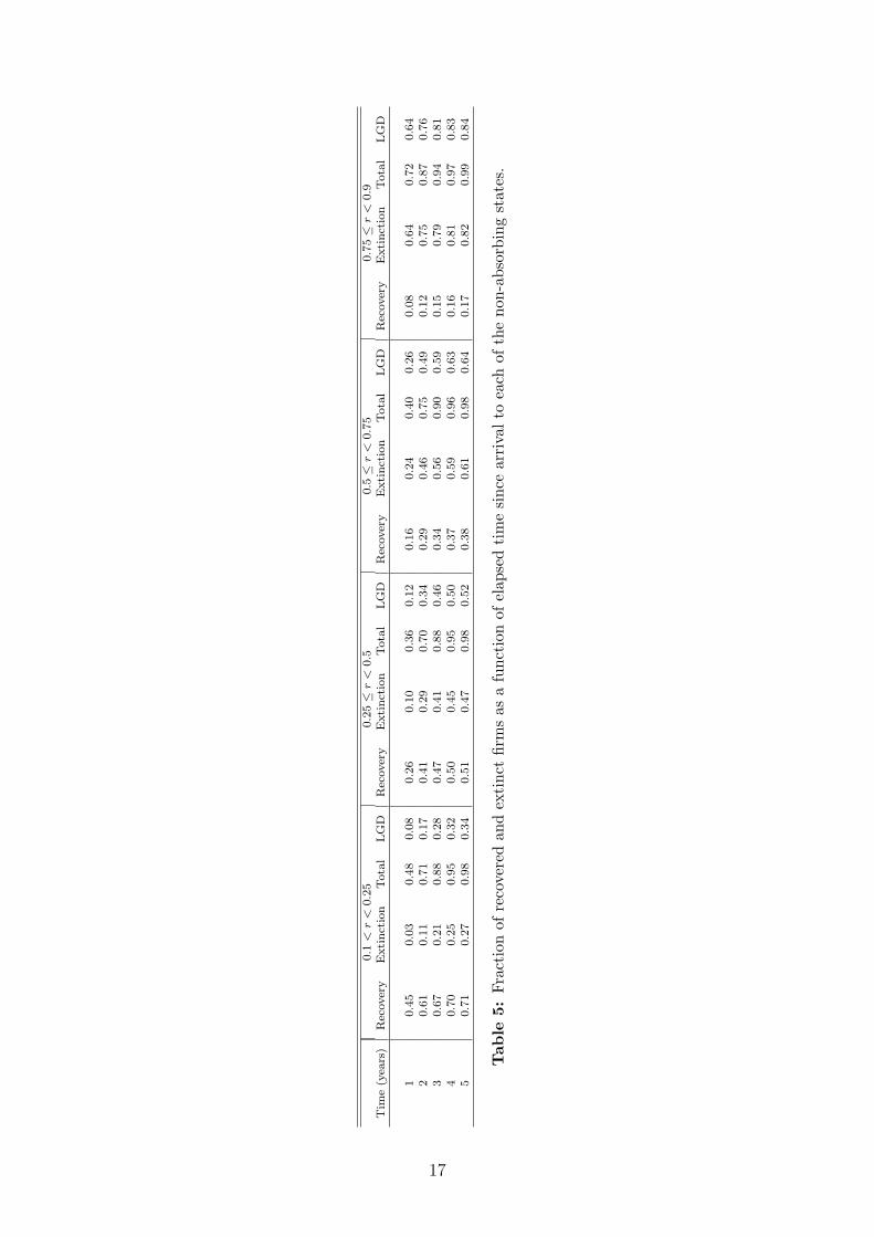
recovery to be revealed. Table 5 presents the fraction of firms that transited to one of

the absorbing states for different time lengths, along with the split between recovery and

extinction, conditional on the event that at time zero they enter one of the non-absorbing

states. For instance, we see that the fate of a firm that at time zero entered state 3 (with

0.1 < r < 0.25) is known with a probability of 48 percent after one year of entering that

state. (As in figure 3, this probability is not conditional on the firm staying in the same

state until transition to recovery or extinction occurs.) At the end of the second year, the

probability that the final outcome has unravelled is 71 percent. In both cases, recovery is

the most likely destination, although less so in the second year.

The calculation of a general purpose LGD involves the integration of probabilities such

as the ones presented in table 5 across all firms that historically have defaulted, conditional

on the firms characteristics. This measure would then be the average loss given default.

This general purpose value is, in the “foundation” of the IRB method, 50 percent. A

rough estimate of a similar value for the data in this work implies an LGD of 46 percent.2

This value seems to support the IRB foundation approach recommendations, but more

accurate values may be easily obtained using the historical distributions of particular loan

portfolios.

However, care must be used when assessing these values. First, data correspond

to a particular time period and to a particular country. Second, the more sophisticated

“advanced” approach encourages a more targeted estimation of LGD, and this is precisely

what this model mainly does.

2This estimate was obtained using the relative frequencies of the first visit to each state found in thedata and the asymptotic values of LGD measures reported in table 5. This value should be viewed as anupper bound because it uses the baseline hazard functions (with all covariates equal to zero) and largerfirms tend to display better outcomes.

16

0.1

<r

<0.2

50.2

5≤

r<

0.5

0.5≤

r<

0.7

50.7

5≤

r<

0.9

Tim

e(y

ears

)R

ecover

yE

xtinct

ion

Tota

lLG

DR

ecover

yE

xtinct

ion

Tota

lLG

DR

ecover

yE

xtinct

ion

Tota

lLG

DR

ecover

yE

xtinct

ion

Tota

lLG

D

10.4

50.0

30.4

80.0

80.2

60.1

00.3

60.1

20.1

60.2

40.4

00.2

60.0

80.6

40.7

20.6

42

0.6

10.1

10.7

10.1

70.4

10.2

90.7

00.3

40.2

90.4

60.7

50.4

90.1

20.7

50.8

70.7

63

0.6

70.2

10.8

80.2

80.4

70.4

10.8

80.4

60.3

40.5

60.9

00.5

90.1

50.7

90.9

40.8

14

0.7

00.2

50.9

50.3

20.5

00.4

50.9

50.5

00.3

70.5

90.9

60.6

30.1

60.8

10.9

70.8

35

0.7

10.2

70.9

80.3

40.5

10.4

70.9

80.5

20.3

80.6

10.9

80.6

40.1

70.8

20.9

90.8

4

Tab

le5:

Frac

tion

ofre

cove

red

and

exti

nct

firm

sas

afu

ncti

onof

elap

sed

tim

esi

nce

arri

valto

each

ofth

eno

n-ab

sorb

ing

stat

es.

17

0 5 10 15 200

0.2

0.4

0.6

0.8

1

Elapsed time (in quarters)

Fra

ctio

n of

firm

s gi

ven

initi

al s

tate

0.1 < r < 0.25

RecoveryExtinction

0 5 10 15 200

0.2

0.4

0.6

0.8

1

Elapsed time (in quarters)

Fra

ctio

n of

firm

s gi

ven

initi

al s

tate

0.25 ≤ r < 0.5

RecoveryExtinction

0 5 10 15 200

0.2

0.4

0.6

0.8

1

Elapsed time (in quarters)

Fra

ctio

n of

firm

s gi

ven

initi

al s

tate

0.5 ≤ r < 0.75

RecoveryExtinction

0 5 10 15 200

0.2

0.4

0.6

0.8

1

Elapsed time (in quarters)

Fra

ctio

n of

firm

s gi

ven

initi

al s

tate

0.75 ≤ r < 0.9

RecoveryExtinction

Figure 3: Fraction of firms that recovered or became extinct given initial state. The resultsare obtained simulating 100000 firms for each initial state.

These results suggest that loss given default calculated over a one year interval, for

instance, is likely to be a short-sighted measure, as a lot of uncertainty regarding recovery

or extinction unravels during the second and third years. Table 5 reports upper bounds

for expected loss given default (LGD) conditional on the initial state, calculated as the

probability of extinction times 100 percent of loss plus the probability of recovery times

10 percent of loss (the lower bound of state 3). Let us focus on state 3, which corresponds

to the default ratio lying between 10 and 25 percent. Suppose a firm that at time zero

defaults and enters state 3. The model estimates that there is a probability of 45 percent

that it recovers in the ensuing year. Conversely, it has a probability of extinction in that

period of 3 percent. Therefore, one would expect that, on average, no less than 8 percent

of total outstanding loans would be lost in a one-year horizon. However, as previously

remarked, during the first year many firms recover and a relatively lower number of firms

go bankrupt. This implies that at time zero the expected loss during the second year

given that the final fate of the firm has not yet been resolved by then is 32 percent of

18

outstanding loans.3 The second year is much more critical in terms of losses than the

first one. A reasonable value for the expected loss horizon is three years: by the end of

the third year of the episode, conditional on initial state 3, the expected three-year loss

is over 80 percent its value in the infinite horizon, and much more than that for the other

initial states.

From a financial supervision viewpoint, it may be preferable to update expected losses

and other measures of firm creditworthiness as time unfolds. This can be done by con-

ditioning these measures to the event that the firm has stayed in the current state for a

given number of quarters, and to the covariates of the firm. Changing covariates will be

the subject of the next section. As for the duration of stay in the current state, figure

4 shows the same type of probability as figure 3 but conditional on the event that the

firm is in a particular non-absorbing state at the end of the first year since entering that

state. Recall the previous observation that the semi-Markov process that we used could

in a first approximation be substituted by a simple Markov chain, that is, a process where

the likelihood of transition does not depend on the duration of stay in the current state.

Consistent with that, figure 4 is not fundamentally different from figure 3, except that

uncertainty regarding the ultimate fate of firms is revealed earlier. For instance, from the

tenth quarter on all probabilities have attained their asymptotic values; this compares

with at least 16 quarters in the previous case. This feature is relevant for estimation of

the expected loss of firms whose history in the current state is known and for which up-

dates are performed regularly. Since for those firms uncertainty unravels faster, estimates

of their expected losses are likely to be more accurate.

4.2 Heterogeneity of firms

Up to this point, we used the so called “baseline hazards” in the estimation of the transi-

tion probabilities and in-state survival times. This section explores another dimension of

the data: the information provided by the internal database.

3This figure may calculated from table 5: there is a 16 percent probability that the firm recoversduring the second year, and an 8 percent probability that it goes to extinction in that period. Thisimplies an LGD measure of 32 percent.

19

0 5 10 15 200

0.2

0.4

0.6

0.8

1

Elapsed time (in quarters)

Fra

ctio

n of

firm

s gi

ven

initi

al s

tate

0.1 < r < 0.25

RecoveryExtinction

0 5 10 15 200

0.2

0.4

0.6

0.8

1

Elapsed time (in quarters)

Fra

ctio

n of

firm

s gi

ven

initi

al s

tate

0.25 ≤ r < 0.5

RecoveryExtinction

0 5 10 15 200

0.2

0.4

0.6

0.8

1

Elapsed time (in quarters)

Fra

ctio

n of

firm

s gi

ven

initi

al s

tate

0.5 ≤ r < 0.75

RecoveryExtinction

0 5 10 15 200

0.2

0.4

0.6

0.8

1

Elapsed time (in quarters)

Fra

ctio

n of

firm

s gi

ven

initi

al s

tate

0.75 ≤ r < 0.9

RecoveryExtinction

Figure 4: Fraction of firms that recovered or became extinct given current state and the factthat the firm entered the current state one year before. The results are obtained simulating100000 firms for each initial state.

Recall from section 2 that the hazard function hik(t|x) is the probability density that

a firm goes from state i to state k 6= i at time t, conditional on the firm entering state i

at time 0, remaining there up to time t, and being characterized by a vector of covariates

x in that period. The proportional hazards hypothesis states that hik(t|x) = exβhik(t),

where hik(t) is the baseline hazard. Therefore, the previous calculations pertain to a firm

for which all covariates are zero. This means a firm without employees or sales, with

outstanding credits d between 104 and 105 euros, with a default episode beginning in

1995, located in the Lisbon region and operating in the commerce and services sector.

It is clear that the first two figures are unrealistic; they could be substituted by, say, 10

employees and sales of 1 million euros without any qualitative difference in the results

hitherto reported.

To compare the impact of the different covariates in the calculations of probabilities

of extinction and recovery, let us define one benchmark case in terms of the number

of employees and sales. We shall consider a firm with 20 employees and annual sales

20

of 1 million euros.4 The other covariates are zero; the hazard functions used therefore

correspond to the omitted categories indicated above.

Perhaps one of the most relevant questions is knowing if the scale of the firm has an

impact on the recovery/extinction time profile. Figure 5 presents the fraction of firms

that recover or become extinct conditional on the initial state. For the least severe cases,

extinction is quite slow and the asymptotic probability of extinction is much lower than

the reference case. Moreover, recovery is slower and more firms end up recovering than

in the reference case. For the most severe cases, the previous conclusions also hold:

uncertainty tends to unravel more slowly for larger firms, generally with a more benign

outcome.

0 2 4 6 8 10 12 14 16 18 200

0.2

0.4

0.6

0.8

1

Elapsed time (in quarters)

Fra

ctio

n of

firm

s gi

ven

initi

al s

tate

0.1 < r < 0.25

Recovery (ref. firm)Extinction (ref. firm)RecoveryExtinction

0 2 4 6 8 10 12 14 16 18 200

0.2

0.4

0.6

0.8

1

Elapsed time (in quarters)

Fra

ctio

n of

firm

s gi

ven

initi

al s

tate

0.75 ≤ r < 0.9

Recovery (ref. firm)Extinction (ref. firm)RecoveryExtinction

Figure 5: Fraction of firms that recovered or became extinct given initial state. Comparisonbetween the reference firm and an identical firm ten times as large as the reference firm. Theresults are obtained simulating 100000 firms for each initial state.

To understand the determinants of the previous behavior, one might resort to the

assessment of the contribution of each of the three variables related to dimension in the

database: number of employees, sales and total outstanding loans. Let us first compare

4The average number of employees and total sales with pooled data are 18.3 and 1.28 million euros,respectively.

21

the benchmark firm with an equal firm except that the number of employees is ten times as

large. Figure 6 shows the result of the exercise. The first observation is that the outcome

is in general more favorable. For the least severe cases, we see that extinction displays

quite different results, since now extinction is faster than the reference case. Recovery is

quite similar. For more severe cases, recovery shows a relatively comparable pattern, but

extinction is faster than the reference case. When we perform the same exercise for firms

with ten times the sales of the reference case (figure 7), we see almost identical patterns

for the least severe cases, and also a qualitatively similar pattern for the most severe

cases with more benign outcomes (lower probability of extinction; higher probability of

recovery). Figure 8 presents the case where outstanding loans are ten times as high as

the reference case. Again, a pattern quite similar to the reference case.

The previous observations suggest that the number of employees in an important

determinant of the time profile of a troubled firm’s extinction/recovery process. Firms

with more employees tend to have more benign outcomes. For the most severe cases, the

recovery process tends to be slower, and the extinction process is faster. For the least

severe cases, extinction is faster but less likely, and recovery is basically more likely. These

facts corroborate a number of both empirical and theoretical studies stating that larger

firms (which tend to have larger sunk costs and specific capital) are more prone to survive

crisis than their smaller counterparts. For instance, Mata and Portugal (1994) find that

the survival of new firms is positively related to a larger dimension in terms of the number

of employees.

5 Conclusions

This paper analyzes the behavior of firms with defaulted credits in terms of recovery or

extinction. By defining classes for the severity of default, survival models for the multiple

transitions from each class are estimated. The models are used to simulate the evolution

of a firm’s situation conditional on the firm’s characteristics. We show that the severity of

default strongly influences the probability of extinction; for less severe default episodes,

recovery is faster than extinction, and the opposite is true for more severe defaults; larger

22

0 2 4 6 8 10 12 14 16 18 200

0.2

0.4

0.6

0.8

1

Elapsed time (in quarters)

Fra

ctio

n of

firm

s gi

ven

initi

al s

tate

0.1 < r < 0.25

Recovery (ref. firm)Extinction (ref. firm)Recovery (more employees)Extinction (more employees)

0 2 4 6 8 10 12 14 16 18 200

0.2

0.4

0.6

0.8

1

Elapsed time (in quarters)

Fra

ctio

n of

firm

s gi

ven

initi

al s

tate

0.75 ≤ r < 0.9

Recovery (ref. firm)Extinction (ref. firm)Recovery (more employees)Extinction (more employees)

Figure 6: Fraction of firms that recovered or became extinct given initial state. Comparisonbetween the reference firm and another firm with ten times the reference firm’s employees. Theresults are obtained simulating 100000 firms for each initial state.

firms tend to display better outcomes; and the number of employees is the single most

important determinant of the time profile of the extinction/recovery process. Estimates of

loss given default corroborate the supervision recommendations regarding this measure.

Within the scope of feasible future improvements of this research, we would empha-

size the introduction of industry-wide and equity measures in the regressions. These

would control for intra-industry competition, relative performance of the industry, and

the impact of foreign ownership and capital structure on the firm performance.

Another improvement, unfortunately not feasible with current data, would be to disag-

gregate credit by credit institution and maturity. This would allow for a proper treatment

of the dynamics of a firm’s credit across financial institutions. An additional piece of in-

teresting information would be the existence or not of collateral.

23

0 2 4 6 8 10 12 14 16 18 200

0.2

0.4

0.6

0.8

1

Elapsed time (in quarters)

Fra

ctio

n of

firm

s gi

ven

initi

al s

tate

0.1 < r < 0.25

Recovery (ref. firm)Extinction (ref. firm)RecoveryExtinction

0 2 4 6 8 10 12 14 16 18 200

0.2

0.4

0.6

0.8

1

Elapsed time (in quarters)

Fra

ctio

n of

firm

s gi

ven

initi

al s

tate

0.75 ≤ r < 0.9

Recovery (ref. firm)Extinction (ref. firm)RecoveryExtinction

Figure 7: Fraction of firms that recovered or became extinct given initial state. Comparisonbetween the reference firm and another firm with ten times the reference firm’s sales. The resultsare obtained simulating 100000 firms for each initial state.

References

Basel Committee on Banking Supervision (2001), The Internal Ratings-Based approach,

Consultative document, Bank for International Settlements.

Basel Committee on Banking Supervision (2004), International convergence of capital

measurement and capital standards, Report, Bank for International Settlements.

Grambsch, P. M. and Therneau, T. M. (1994), ‘Proportional hazards tests and diagnostics

based on weighted residuals’, Biometrika 81, 515–526.

Lancaster, T. (1992), The Econometric Analysis of Transition Data, Econometric Society

Monographs, Cambridge University Press.

Mata, J. and Portugal, P. (1994), ‘Life duration of new firms’, Journal of Industrial

Economics 42(3), 227–245.

24

0 2 4 6 8 10 12 14 16 18 200

0.2

0.4

0.6

0.8

1

Elapsed time (in quarters)

Fra

ctio

n of

firm

s gi

ven

initi

al s

tate

0.1 < r < 0.25

Recovery (ref. firm)Extinction (ref. firm)RecoveryExtinction

0 2 4 6 8 10 12 14 16 18 200

0.2

0.4

0.6

0.8

1

Elapsed time (in quarters)

Fra

ctio

n of

firm

s gi

ven

initi

al s

tate

0.75 ≤ r < 0.9

Recovery (ref. firm)Extinction (ref. firm)RecoveryExtinction

Figure 8: Fraction of firms that recovered or became extinct given initial state. Comparisonbetween the reference firm and another firm with outstanding loans between 1000 and 10000euros. The results are obtained simulating 100000 firms for each initial state.

Appendix A Sensitivity to thresholds

An important issue in this approach is the impact of the thresholds for the definition of

states, especially the absorbing ones, on the statistical significance and accuracy of the

estimates. An extensive analysis was performed with respect to their definition. Here we

report the results for the most important threshold, the upper limit of the default ratio of

the absorbing state “recovery”, which was set at 10 percent. Figure 9 displays the median

extinction probabilities for states 3 and 6 conditional on the current state and the length of

stay in the current state. We see in panel (b) that setting a much more stringent threshold

(5 percent) yields qualitatively similar results, but the confidence intervals at 90 percent

become a lot wider. This is due to the fact that for a more stringent threshold we end up

having much less transitions to recovery and any estimates are bound to become much

less accurate. This result suggests that using more stringent thresholds does not change

significantly the median results, but does severely affect their accuracy. As a consequence,

25

the probability of extinction for state 6 is statistically higher at the 5 percent level than

that of state 3, for example.

1 2 3 4 5 60

0.2

0.4

0.6

0.8

1

Quarters in the current state

Pro

babi

lity

of e

xtin

ctio

nState: 0.1< r < 0.25

1 2 3 4 5 60

0.2

0.4

0.6

0.8

1

Quarters in the current state

(a) Lower limit equal to 0.1

Pro

babi

lity

of e

xtin

ctio

n

State: 0.75 ≤ r < 0.9

1 2 3 4 5 60

0.2

0.4

0.6

0.8

1

Quarters in the current state

Pro

babi

lity

of e

xtin

ctio

n

State: 0.05 < r < 0.25

1 2 3 4 5 60

0.2

0.4

0.6

0.8

1

Quarters in the current state

(b) Lower limit equal to 0.05

Pro

babi

lity

of e

xtin

ctio

n

State: 0.75 ≤ r < 0.9

Figure 9: Median extinction probabilities for two states and two different values of the lowerlimit of r, with 90 percent confidence intervals. Results using 100 simulated firms per each of1000 parameter draws.

26

Appendix B Regressions results

27

(1) (2) (3) (4) (5) (6) (7)(3→ 1) (3→ 2) (3→ 4) (3→ 5) (3→ 6) (4→ 1) (4→ 2)

Employees (102) -0.003 0.207 -0.327 -0.144 0.170 -0.046 -0.547(0.03) (0.73) (2.16)* (0.34) (0.93) (0.20) (1.37)

Sales (106) -0.000 -0.214 0.009 -0.023 -0.006 -0.048 0.026(0.05) (1.27) (2.62)** (0.33) (1.17) (1.00) (1.62)

102 ≤ d < 103 -0.486 1.780 0.420 0.104 -10.914 -0.327 1.661(0.84) (3.79)** (0.97) (0.10) (40.33)** (0.78) (6.62)**

103 ≤ d < 104 -0.133 0.763 0.400 -0.006 -0.121 -0.347 1.191(1.47) (4.83)** (4.65)** (0.03) (0.37) (2.37)* (8.89)**

105 ≤ d < 106 0.225 -0.772 -0.010 0.006 -0.186 0.032 -0.312(3.13)** (3.47)** (0.12) (0.03) (0.76) (0.28) (1.85)

d ≥ 106 -0.185 -0.343 0.252 -0.143 -0.503 -0.207 -1.081(1.20) (0.93) (1.61) (0.42) (1.11) (0.76) (2.37)*

Year 1996 0.021 0.410 -0.154 -0.317 -0.135 0.095 0.083(0.20) (1.68) (1.29) (1.43) (0.39) (0.54) (0.43)

Year 1997 -0.140 0.505 0.033 0.037 0.041 0.148 0.278(1.33) (2.07)* (0.30) (0.18) (0.12) (0.87) (1.51)

Year 1998 0.028 0.289 -0.094 -0.287 0.090 0.190 0.063(0.26) (1.13) (0.80) (1.29) (0.27) (1.10) (0.32)

Year 1999 0.030 0.177 -0.100 -0.635 -0.590 0.204 -0.184(0.29) (0.68) (0.87) (2.53)* (1.46) (1.17) (0.87)

Year 2000 -0.179 -0.326 -0.388 -0.515 -0.107 -0.094 -0.799(1.50) (0.98) (2.78)** (1.86) (0.26) (0.44) (2.66)**

Primary activities 0.043 0.726 -0.048 -0.310 1.031 0.014 0.257(0.24) (1.89) (0.20) (0.65) (2.09)* (0.06) (0.72)

Extraction and manufacturing -0.091 0.149 0.363 -0.202 1.144 0.123 -0.112(0.70) (0.65) (2.83)** (0.81) (3.92)** (0.68) (0.48)

Wood, chemistry, machinery 0.175 -0.507 0.202 -0.348 0.203 0.072 0.271(1.70) (1.87) (1.80) (1.44) (0.54) (0.47) (1.50)

Electric instruments -0.191 -0.008 -0.033 -0.444 -0.950 -0.309 -0.488(1.00) (0.02) (0.18) (1.07) (0.92) (0.84) (1.11)

Utilities and construction 0.066 0.003 0.164 -0.111 0.354 0.030 0.335(0.66) (0.01) (1.45) (0.51) (0.95) (0.18) (1.82)

Transportation 0.037 -0.453 0.125 -0.801 0.544 0.234 0.356(0.26) (1.14) (0.81) (1.90) (1.19) (1.08) (1.43)

Services to firms and housing 0.151 -0.307 0.037 -0.326 -0.116 0.116 -0.019(1.19) (1.05) (0.25) (1.16) (0.23) (0.61) (0.08)

Education and health care 0.100 0.388 0.224 -1.565 0.834 -0.107 0.145(0.47) (0.98) (0.98) (1.55) (1.35) (0.31) (0.38)

Collective and social services -0.305 0.201 -0.337 0.353 -0.034 -0.018 0.160(1.38) (0.53) (1.19) (1.00) (0.04) (0.06) (0.46)

North 0.170 0.167 0.059 0.213 -0.260 0.053 0.195(2.18)* (0.99) (0.68) (1.33) (1.00) (0.44) (1.43)

Center 0.220 0.039 0.201 0.063 0.135 0.181 -0.171(2.29)* (0.19) (1.97)* (0.31) (0.46) (1.31) (0.98)

Alentejo 0.038 -0.338 -0.391 -0.811 -0.218 -0.013 -0.195(0.26) (0.93) (1.95) (1.73) (0.38) (0.05) (0.66)

Algarve 0.283 0.338 0.033 0.586 0.416 -0.177 -0.072(1.79) (1.00) (0.17) (1.88) (0.91) (0.72) (0.28)

Constant -2.662 -4.608 -2.971 -3.942 -5.404 -3.205 -4.031(26.95)** (19.35)** (28.14)** (19.41)** (16.43)** (18.65)** (20.82)**

Observations 10156 10156 10156 10156 10156 7422 7422Subjects 7391.00 7391.00 7391.00 7391.00 7391.00 5127.00 5127.00

Transitions 1336.00 227.00 1027.00 234.00 91.00 510.00 348.00α 1.80 1.93 1.94 1.84 1.96 1.62 1.87

Table 6: Maximum likelihood estimation results. Omitted categories are: outstanding loans dbetween 104 and 105 euros; year of arrival to state 1995; commerce and services sector; Lisbonregion.

28

(8) (9) (10) (11) (12) (13) (14)(4→ 3) (4→ 5) (4→ 6) (5→ 1) (5→ 2) (5→ 3) (5→ 4)

Employees (102) 0.253 -0.173 -0.849 0.876 -0.455 -0.070 0.242(1.31) (0.71) (1.44) (3.62)** (1.21) (0.16) (1.07)

Sales (106) -0.012 0.008 -0.008 -0.053 0.018 -0.003 -0.010(1.19) (0.78) (0.20) (1.42) (1.21) (0.04) (1.16)

102 ≤ d < 103 -0.616 -0.213 0.875 0.176 1.312 -0.361 -15.075(1.35) (0.56) (2.11)* (0.30) (5.29)** (0.50) (90.30)**

103 ≤ d < 104 -0.071 0.482 -0.261 -0.505 1.171 -0.551 0.029(0.56) (4.48)** (1.02) (1.70) (9.59)** (1.85) (0.17)

105 ≤ d < 106 -0.278 -0.048 0.028 -0.106 -0.617 -0.365 -0.467(2.40)* (0.42) (0.14) (0.54) (3.67)** (1.66) (2.90)**

d ≥ 106 -0.365 0.131 0.357 -1.264 -0.721 -0.668 -0.554(1.60) (0.61) (0.83) (2.62)** (1.97)* (1.44) (1.68)

Year 1996 0.011 -0.051 0.217 -0.329 0.098 -0.121 -0.088(0.07) (0.34) (0.85) (1.13) (0.53) (0.40) (0.43)

Year 1997 -0.199 0.015 -0.326 -0.114 0.073 -0.216 -0.128(1.20) (0.10) (1.17) (0.41) (0.40) (0.70) (0.60)

Year 1998 -0.085 -0.219 -0.336 0.169 0.259 0.041 0.077(0.51) (1.35) (1.15) (0.61) (1.43) (0.14) (0.38)

Year 1999 0.142 -0.019 -0.320 -0.370 0.395 -0.242 -0.163(0.89) (0.12) (1.07) (1.18) (2.22)* (0.76) (0.75)

Year 2000 -0.281 -0.147 -0.330 -0.218 0.008 -0.207 -0.285(1.40) (0.81) (0.92) (0.62) (0.04) (0.56) (1.07)

Primary activities 0.103 -0.820 -0.144 0.018 0.046 -0.267 0.247(0.42) (2.31)* (0.32) (0.04) (0.13) (0.46) (0.64)

Extraction and manufacturing -0.207 0.094 -0.076 -0.304 0.280 -0.178 0.266(1.13) (0.59) (0.25) (0.95) (1.45) (0.55) (1.29)

Wood, chemistry, machinery 0.036 -0.004 0.351 0.104 -0.146 -0.127 -0.151(0.24) (0.03) (1.46) (0.38) (0.73) (0.42) (0.66)

Electric instruments -0.493 0.017 -0.317 -0.376 0.288 0.299 0.303(1.27) (0.05) (0.56) (0.77) (1.07) (0.68) (0.91)

Utilities and construction 0.195 0.059 -0.334 0.013 0.103 0.076 0.203(1.28) (0.41) (1.13) (0.05) (0.60) (0.27) (1.04)

Transportation 0.078 0.087 0.344 -0.495 0.172 -1.420 0.283(0.36) (0.44) (0.99) (1.01) (0.78) (1.94) (1.01)

Services to firms and housing -0.067 0.001 -0.537 0.305 0.091 0.204 0.131(0.35) (0.00) (1.34) (1.01) (0.41) (0.60) (0.49)

Education and health care 0.099 -0.193 -14.533 -0.680 0.479 -0.633 -0.135(0.32) (0.62) (71.56)** (0.67) (1.52) (0.62) (0.23)

Collective and social services -0.005 0.009 -0.901 -0.066 0.890 -0.280 0.987(0.02) (0.04) (1.20) (0.12) (3.65)** (0.39) (3.49)**

North -0.109 -0.053 -0.157 0.120 0.025 0.011 0.225(0.96) (0.49) (0.82) (0.57) (0.19) (0.05) (1.45)

Center -0.082 0.064 -0.283 0.298 0.342 0.121 0.078(0.60) (0.51) (1.13) (1.21) (2.42)* (0.45) (0.41)

Alentejo 0.146 -0.375 -1.119 -0.052 -0.352 0.698 0.740(0.70) (1.64) (1.84) (0.10) (0.97) (1.72) (2.56)*

Algarve -0.658 -0.129 -0.500 0.264 0.143 -0.370 0.297(2.39)* (0.63) (1.14) (0.79) (0.59) (0.78) (1.11)

Constant -2.851 -2.985 -3.831 -3.636 -3.338 -3.451 -3.128(19.12)** (20.84)** (14.04)** (14.16)** (18.60)** (12.99)** (16.48)**

Observations 7422 7422 7422 4098 4098 4098 4098Subjects 5127.00 5127.00 5127.00 2853.00 2853.00 2853.00 2853.00

Transitions 552.00 650.00 162.00 158.00 439.00 142.00 302.00α 1.68 1.79 1.66 1.71 1.99 1.67 1.72

Table 6: Continued.

29

(15) (16) (17) (18) (19) (20)(5→ 6) (6→ 1) (6→ 2) (6→ 3) (6→ 4) (6→ 5)

Employees (102) -0.224 -0.983 0.585 1.648 0.269 0.413(0.76) (1.08) (1.93) (2.87)** (0.36) (1.03)

Sales (106) 0.009 0.038 -0.026 -0.084 -0.006 -0.069(0.80) (1.05) (1.96) (1.29) (0.22) (0.88)

102 ≤ d < 103 -0.930 0.069 0.606 0.140 0.540 -13.342(1.28) (0.09) (2.15)* (0.14) (0.67) (48.49)**

103 ≤ d < 104 0.454 -0.218 0.456 0.602 0.464 -0.054(3.14)** (0.58) (3.61)** (1.47) (1.25) (0.21)

105 ≤ d < 106 -0.220 -0.302 -0.314 -1.689 -0.330 -0.066(1.44) (1.02) (2.03)* (2.84)** (0.90) (0.30)

d ≥ 106 -0.066 -1.339 -0.814 -2.305 -0.437 -0.189(0.24) (1.61) (2.78)** (2.17)* (0.81) (0.45)

Year 1996 -0.057 0.027 -0.393 0.246 0.613 -0.283(0.30) (0.06) (2.16)* (0.27) (1.02) (0.99)

Year 1997 -0.228 0.304 0.038 1.206 0.720 -0.270(1.18) (0.68) (0.24) (1.48) (1.17) (0.91)

Year 1998 -0.149 0.340 -0.216 1.090 1.089 -0.261(0.74) (0.75) (1.21) (1.30) (1.88) (0.90)

Year 1999 0.021 0.005 -0.356 1.131 0.900 -0.442(0.11) (0.01) (1.99)* (1.33) (1.53) (1.46)

Year 2000 -0.581 0.040 -0.615 1.317 -0.188 -1.258(2.15)* (0.07) (2.57)* (1.49) (0.21) (2.31)*

Primary activities -1.172 -0.510 -0.116 1.719 0.482 -1.962(1.81) (0.66) (0.38) (2.40)* (0.78) (1.92)

Extraction and manufacturing 0.323 -0.664 -0.312 -2.009 -1.069 0.057(1.66) (1.20) (1.40) (2.50)* (1.58) (0.18)

Wood, chemistry, machinery 0.275 -0.053 -0.143 -0.723 0.478 0.342(1.48) (0.12) (0.77) (0.88) (1.21) (1.30)

Electric instruments 0.640 -0.648 -0.475 -14.247 0.231 0.196(2.26)* (0.89) (1.15) (25.55)** (0.39) (0.39)

Utilities and construction 0.212 0.172 -0.094 0.888 0.407 0.080(1.12) (0.46) (0.49) (1.68) (1.02) (0.26)

Transportation -0.079 -0.284 0.044 -0.390 -0.304 0.142(0.29) (0.44) (0.21) (0.37) (0.40) (0.35)

Services to firms and housing 0.164 -0.562 -0.244 0.747 -0.794 -0.339(0.68) (1.04) (1.14) (1.35) (1.12) (0.80)

Education and health care -0.003 1.029 0.111 -13.554 0.363 -0.774(0.01) (1.58) (0.35) (29.63)** (0.35) (0.74)

Collective and social services 0.114 0.505 -0.393 0.689 -13.553 0.669(0.27) (0.81) (0.88) (0.58) (39.26)** (1.29)

North 0.141 0.269 0.028 0.778 0.115 -0.105(0.99) (0.88) (0.21) (1.79) (0.35) (0.48)

Center 0.369 -0.002 -0.112 -0.076 -0.573 0.190(2.31)* (0.01) (0.71) (0.12) (1.27) (0.74)

Alentejo 0.266 -13.704 -0.205 1.386 0.413 -0.251(0.80) (29.61)** (0.57) (2.14)* (0.67) (0.40)

Algarve 0.049 0.832 -0.545 -0.848 -0.588 0.815(0.16) (1.97)* (1.93) (0.73) (0.76) (2.55)*

Constant -3.130 -3.954 -1.824 -6.005 -4.742 -2.872(18.63)** (9.04)** (11.77)** (6.84)** (8.02)** (10.76)**

Observations 4098 2238 2238 2238 2238 2238Subjects 2853.00 1527.00 1527.00 1527.00 1527.00 1527.00

Transitions 370.00 75.00 454.00 33.00 62.00 151.00α 1.87 1.89 1.80 1.93 1.73 1.65

Table 6: Continued.

30

WORKING PAPERS

2000

1/00 UNEMPLOYMENT DURATION: COMPETING AND DEFECTIVE RISKS

— John T. Addison, Pedro Portugal

2/00 THE ESTIMATION OF RISK PREMIUM IMPLICIT IN OIL PRICES

— Jorge Barros Luís

3/00 EVALUATING CORE INFLATION INDICATORS

— Carlos Robalo Marques, Pedro Duarte Neves, Luís Morais Sarmento

4/00 LABOR MARKETS AND KALEIDOSCOPIC COMPARATIVE ADVANTAGE

— Daniel A. Traça

5/00 WHY SHOULD CENTRAL BANKS AVOID THE USE OF THE UNDERLYING INFLATION INDICATOR?

— Carlos Robalo Marques, Pedro Duarte Neves, Afonso Gonçalves da Silva

6/00 USING THE ASYMMETRIC TRIMMED MEAN AS A CORE INFLATION INDICATOR

— Carlos Robalo Marques, João Machado Mota

2001

1/01 THE SURVIVAL OF NEW DOMESTIC AND FOREIGN OWNED FIRMS

— José Mata, Pedro Portugal

2/01 GAPS AND TRIANGLES

— Bernardino Adão, Isabel Correia, Pedro Teles

3/01 A NEW REPRESENTATION FOR THE FOREIGN CURRENCY RISK PREMIUM

— Bernardino Adão, Fátima Silva

4/01 ENTRY MISTAKES WITH STRATEGIC PRICING

— Bernardino Adão

5/01 FINANCING IN THE EUROSYSTEM: FIXED VERSUS VARIABLE RATE TENDERS

— Margarida Catalão-Lopes

6/01 AGGREGATION, PERSISTENCE AND VOLATILITY IN A MACROMODEL

— Karim Abadir, Gabriel Talmain

7/01 SOME FACTS ABOUT THE CYCLICAL CONVERGENCE IN THE EURO ZONE

— Frederico Belo

8/01 TENURE, BUSINESS CYCLE AND THE WAGE-SETTING PROCESS

— Leandro Arozamena, Mário Centeno

9/01 USING THE FIRST PRINCIPAL COMPONENT AS A CORE INFLATION INDICATOR

José Ferreira Machado, Carlos Robalo Marques, Pedro Duarte Neves, Afonso Gonçalves da Silva

10/01 IDENTIFICATION WITH AVERAGED DATA AND IMPLICATIONS FOR HEDONIC REGRESSION STUDIES

— José A.F. Machado, João M.C. Santos Silva

2002

1/02 QUANTILE REGRESSION ANALYSIS OF TRANSITION DATA

— José A.F. Machado, Pedro Portugal

2/02 SHOULD WE DISTINGUISH BETWEEN STATIC AND DYNAMIC LONG RUN EQUILIBRIUM IN ERROR

CORRECTION MODELS?

— Susana Botas, Carlos Robalo Marques

Banco de Portugal / Working Papers i

3/02 MODELLING TAYLOR RULE UNCERTAINTY

— Fernando Martins, José A. F. Machado, Paulo Soares Esteves

4/02 PATTERNS OF ENTRY, POST-ENTRY GROWTH AND SURVIVAL: A COMPARISON BETWEEN DOMESTIC

AND FOREIGN OWNED FIRMS

— José Mata, Pedro Portugal

5/02 BUSINESS CYCLES: CYCLICAL COMOVEMENT WITHIN THE EUROPEAN UNION IN THE PERIOD

1960-1999. A FREQUENCY DOMAIN APPROACH

— João Valle e Azevedo

6/02 AN “ART”, NOT A “SCIENCE”? CENTRAL BANK MANAGEMENT IN PORTUGAL UNDER THE GOLD

STANDARD, 1854-1891

— Jaime Reis

7/02 MERGE OR CONCENTRATE? SOME INSIGHTS FOR ANTITRUST POLICY

— Margarida Catalão-Lopes

8/02 DISENTANGLING THE MINIMUM WAGE PUZZLE: ANALYSIS OF WORKER ACCESSIONS AND

SEPARATIONS FROM A LONGITUDINAL MATCHED EMPLOYER-EMPLOYEE DATA SET

— Pedro Portugal, Ana Rute Cardoso

9/02 THE MATCH QUALITY GAINS FROM UNEMPLOYMENT INSURANCE

— Mário Centeno

10/02 HEDONIC PRICES INDEXES FOR NEW PASSENGER CARS IN PORTUGAL (1997-2001)

— Hugo J. Reis, J.M.C. Santos Silva

11/02 THE ANALYSIS OF SEASONAL RETURN ANOMALIES IN THE PORTUGUESE STOCK MARKET

— Miguel Balbina, Nuno C. Martins

12/02 DOES MONEY GRANGER CAUSE INFLATION IN THE EURO AREA?

— Carlos Robalo Marques, Joaquim Pina

13/02 INSTITUTIONS AND ECONOMIC DEVELOPMENT: HOW STRONG IS THE RELATION?

— Tiago V.de V. Cavalcanti, Álvaro A. Novo

2003

1/03 FOUNDING CONDITIONS AND THE SURVIVAL OF NEW FIRMS

— P.A. Geroski, José Mata, Pedro Portugal

2/03 THE TIMING AND PROBABILITY OF FDI:

An Application to the United States Multinational Enterprises

— José Brandão de Brito, Felipa de Mello Sampayo

3/03 OPTIMAL FISCAL AND MONETARY POLICY: EQUIVALENCE RESULTS

— Isabel Correia, Juan Pablo Nicolini, Pedro Teles

4/03 FORECASTING EURO AREA AGGREGATES WITH BAYESIAN VAR AND VECM MODELS

— Ricardo Mourinho Félix, Luís C. Nunes

5/03 CONTAGIOUS CURRENCY CRISES: A SPATIAL PROBIT APPROACH

— Álvaro Novo

6/03 THE DISTRIBUTION OF LIQUIDITY IN A MONETARY UNION WITH DIFFERENT PORTFOLIO RIGIDITIES

— Nuno Alves

7/03 COINCIDENT AND LEADING INDICATORS FOR THE EURO AREA: A FREQUENCY BAND APPROACH

— António Rua, Luís C. Nunes

8/03 WHY DO FIRMS USE FIXED-TERM CONTRACTS?

— José Varejão, Pedro Portugal

9/03 NONLINEARITIES OVER THE BUSINESS CYCLE: AN APPLICATION OF THE SMOOTH TRANSITION

AUTOREGRESSIVE MODEL TO CHARACTERIZE GDP DYNAMICS FOR THE EURO-AREA AND PORTUGAL

— Francisco Craveiro Dias

Banco de Portugal / Working Papers ii

10/03 WAGES AND THE RISK OF DISPLACEMENT

— Anabela Carneiro, Pedro Portugal

11/03 SIX WAYS TO LEAVE UNEMPLOYMENT

— Pedro Portugal, John T. Addison

12/03 EMPLOYMENT DYNAMICS AND THE STRUCTURE OF LABOR ADJUSTMENT COSTS

— José Varejão, Pedro Portugal

13/03 THE MONETARY TRANSMISSION MECHANISM: IS IT RELEVANT FOR POLICY?

— Bernardino Adão, Isabel Correia, Pedro Teles

14/03 THE IMPACT OF INTEREST-RATE SUBSIDIES ON LONG-TERM HOUSEHOLD DEBT:

EVIDENCE FROM A LARGE PROGRAM

— Nuno C. Martins, Ernesto Villanueva

15/03 THE CAREERS OF TOP MANAGERS AND FIRM OPENNESS: INTERNAL VERSUS EXTERNAL LABOUR

MARKETS

— Francisco Lima, Mário Centeno

16/03 TRACKING GROWTH AND THE BUSINESS CYCLE: A STOCHASTIC COMMON CYCLE MODEL FOR THE

EURO AREA

— João Valle e Azevedo, Siem Jan Koopman, António Rua

17/03 CORRUPTION, CREDIT MARKET IMPERFECTIONS, AND ECONOMIC DEVELOPMENT

— António R. Antunes, Tiago V. Cavalcanti

18/03 BARGAINED WAGES, WAGE DRIFT AND THE DESIGN OF THE WAGE SETTING SYSTEM

— Ana Rute Cardoso, Pedro Portugal

19/03 UNCERTAINTY AND RISK ANALYSIS OF MACROECONOMIC FORECASTS:

FAN CHARTS REVISITED

— Álvaro Novo, Maximiano Pinheiro

2004

1/04 HOW DOES THE UNEMPLOYMENT INSURANCE SYSTEM SHAPE THE TIME PROFILE OF JOBLESS

DURATION?

— John T. Addison, Pedro Portugal

2/04 REAL EXCHANGE RATE AND HUMAN CAPITAL IN THE EMPIRICS OF ECONOMIC GROWTH

— Delfim Gomes Neto

3/04 ON THE USE OF THE FIRST PRINCIPAL COMPONENT AS A CORE INFLATION INDICATOR

— José Ramos Maria

4/04 OIL PRICES ASSUMPTIONS IN MACROECONOMIC FORECASTS: SHOULD WE FOLLOW FUTURES MARKET

EXPECTATIONS?

— Carlos Coimbra, Paulo Soares Esteves

5/04 STYLISED FEATURES OF PRICE SETTING BEHAVIOUR IN PORTUGAL: 1992-2001

— Mónica Dias, Daniel Dias, Pedro D. Neves

6/04 A FLEXIBLE VIEW ON PRICES

— Nuno Alves

7/04 ON THE FISHER-KONIECZNY INDEX OF PRICE CHANGES SYNCHRONIZATION

— D.A. Dias, C. Robalo Marques, P.D. Neves, J.M.C. Santos Silva

8/04 INFLATION PERSISTENCE: FACTS OR ARTEFACTS?

— Carlos Robalo Marques

9/04 WORKERS’ FLOWS AND REAL WAGE CYCLICALITY

— Anabela Carneiro, Pedro Portugal

10/04 MATCHING WORKERS TO JOBS IN THE FAST LANE: THE OPERATION OF FIXED-TERM CONTRACTS

— José Varejão, Pedro Portugal

Banco de Portugal / Working Papers iii

11/04 THE LOCATIONAL DETERMINANTS OF THE U.S. MULTINATIONALS ACTIVITIES

— José Brandão de Brito, Felipa Mello Sampayo

12/04 KEY ELASTICITIES IN JOB SEARCH THEORY: INTERNATIONAL EVIDENCE

— John T. Addison, Mário Centeno, Pedro Portugal

13/04 RESERVATION WAGES, SEARCH DURATION AND ACCEPTED WAGES IN EUROPE

— John T. Addison, Mário Centeno, Pedro Portugal

14/04 THE MONETARY TRANSMISSION N THE US AND THE EURO AREA:

COMMON FEATURES AND COMMON FRICTIONS

— Nuno Alves

15/04 NOMINAL WAGE INERTIA IN GENERAL EQUILIBRIUM MODELS

— Nuno Alves

16/04 MONETARY POLICY IN A CURRENCY UNION WITH NATIONAL PRICE ASYMMETRIES

—Sandra Gomes

17/04 NEOCLASSICAL INVESTMENT WITH MORAL HAZARD

—João Ejarque

18/04 MONETARY POLICY WITH STATE CONTINGENT INTEREST RATES

—Bernardino Adão, Isabel Correia, Pedro Teles

19/04 MONETARY POLICY WITH SINGLE INSTRUMENT FEEDBACK RULES

—Bernardino Adão, Isabel Correia, Pedro Teles

20/04 ACOUNTING FOR THE HIDDEN ECONOMY:

BARRIERS TO LAGALITY AND LEGAL FAILURES

—António R. Antunes, Tiago V. Cavalcanti

2005

1/05 SEAM: A SMALL-SCALE EURO AREA MODEL WITH FORWARD-LOOKING ELEMENTS

—José Brandão de Brito, Rita Duarte

2/05 FORECASTING INFLATION THROUGH A BOTTOM-UP APPROACH: THE PORTUGUESE CASE

—Cláudia Duarte, António Rua

3/05 USING MEAN REVERSION AS A MEASURE OF PERSISTENCE

—Daniel Dias, Carlos Robalo Marques

4/05 HOUSEHOLD WEALTH IN PORTUGAL: 1980-2004

—Fátima Cardoso, Vanda Geraldes da Cunha

5/05 ANALYSIS OF DELINQUENT FIRMS USING MULTI-STATE TRANSITIONS

—António Antunes

A

Banco de Portugal / Working Papers iv