Bank Capital and Dividend Externalities

Viral V. Acharya Hanh LeNYU-Stern NYU-Stern

CEPR and NBER hle@stern.nyu.eduvacharya@stern.nyu.edu

Hyun Song ShinPrinceton Universityhsshin@princeton.edu

May 1, 2013

Abstract

While losses were accumulating during the 2007-09 financial crisis, many bankscontinued to maintain a relatively smooth dividend policy. We present a modelthat explains this behavior in a setting where there are financial externalitiesacross banks. In particular, by paying out dividends, a bank transfers value to itsshareholders away from its creditors, who in turn are other banks. This way, onebank’s dividend payout policy affects the equity value and risk of default of otherbanks. When such negative externalities are strong and bank franchise valuesare not too low, the private equilibrium can feature excess dividends relative toa coordinated policy that maximizes the combined equity value of banks.

Keywords: risk-shifting, externalities, franchise value, financial crises.

JEL: G01,G21,G24,G28,G32,G35,G38

1 Introduction

As the financial system’s capital was being depleted, many banks continued to pay

dividends well into the depth of the 2007-2009 financial crisis. Large bank holding

companies such as Bank of America, Citigroup and JP Morgan maintained a smooth

dividend behavior, while securities companies such as Lehman Brothers and Merrill

Lynch even increased their dividends as losses were accumulating. This behavior rep-

resents a type of risk-shifting or asset substitution that favors equity holders over debt

holders (as in the seminal work of Jensen and Meckling, 1976).

We present a simple model where, in the presence of risky debt, risk shifting in-

centives can motivate the payment of dividends as observed during the crisis. In our

model, the bank has assets in place that generate some cash flow in the current period

and some uncertain cash flow in the next period. At any given point in time, the bank

has a franchise value (say, the present value of all its future cash flows) that is largely

determined by the relationship with its customers and counterparties. The bank can

pay dividends out of the current cash flow, and carry the remaining cash to the next

period. The bank has to fulfill non-negotiable debt obligations in the next period out of

the next period’s cash flow and cash savings from the current period. If debt obligations

are not satisfied, the bank is in default. In this case, equity holders receive no value

from the next period cash flow, and furthermore, the bank’s franchise value is lost, for

example, through a disorderly liquidation or transfer to another bank or government.

Given this setup, the first best solution that maximizes the total equity and debt

value of the bank is to pay zero dividends. This is because risk shifting will decrease

the total value of the bank by increasing the probability that its franchise value will be

lost. Any gain from risk shifting by the bank’s equity holders is a loss to its creditors

in a zero sum game. However, we show that in practice when the dividend policy of a

bank is set to maximize its equity holders’ value, the optimal dividend policy can stray

away from the first best solution. Here, the dividend policy reflects a tradeoff between

(i) paying out to equity holders the available cash today rather than transferring it

to creditors in default states in the future; and (ii) saving the equity’s option on the

1

franchise value since dividend payout raises the likelihood of default and thus foregoing

this value. When debt is risky (i.e, when bank leverage is sufficiently high), the optimal

dividend policy depends on the bank’s franchise value. If the franchise value exceeds a

critical threshold, the effect in (ii) dominates and it becomes optimal for the bank not

to pay any dividends. However, if the franchise value is below the critical threshold

such that risk-shifting benefits in (i) become dominant, then the bank would pay out

all available cash as dividends.

The key question is why banks do not find mechanisms ex-ante to guard against

such ex-post agency problems, e.g, by including dividend cutoff or earnings retention

covenants in bank debt contracts. To understand this, we next introduce financial

contracts between two banks, A and B, and analyze how the dividend policy of one

bank creates externalities on the other bank. The connection between the two banks

takes the form of a contingent contract, such as an interest rate or a credit default

swap, under which, in the next period, bank A has to pay bank B an amount in one

state of the world and vice versa in the other state. We show that bank B’s dividends

increase the probability that B will default on its debt obligations to bank A, thereby

exerting negative externalities on bank A’s equity value. In this setup, we show the

complementarity of dividend policies of the two banks. Specifically, when bank B pays

out all available cash as dividends to its equity holders, bank A is more likely to pay

out maximum cash flows since the threshold franchise value under which bank A will

pay maximum dividend is higher when B pays maximum dividends.

Based on this result, we characterize the Nash equilibrium as a two-by-two game

that at high franchise values features no dividend payouts, at low franchise values full

dividend payouts, and for intermediate franchise values multiple equilibria. In this last

case, payoff spillover in the banks’ dividend policies – the fact that dividend payments

by one bank increases the incentives of the other bank to pay out dividends – interferes

with the Nash responses. And as a result, the equilibrium featuring zero dividends by

both banks yields the same private benefits as one featuring maximum dividends. We

refine these multiple equilibria using global game techniques. Specifically, we assume

2

each bank receives a noisy signal of the other bank’s franchise value and define a unique

switching point based on this signal above which both banks pay zero dividends, and

vice versa.

Finally, we characterize the dividend policy that is coordinated and maximizes the

joint equity value of the two banks, where each bank’s dividend “externalities” are

internalized. We show that when externalities are big relative to the private benefits

of paying dividends (i.e, when banks’ franchise values are sufficiently high), the Nash

equilibrium features excessive dividends relative to this policy. Similar to the debt

overhang problem described by Myers (1977), banks do not have an incentive to curb

excessive dividends, as the benefits accrue only to their creditors who in turn are their

interconnected entities.

Dividend regulation, therefore, arises as a desirable intervention due to the lack of

coordination between equity holders of different banks. Restrictions on dividends can

make equity claims of both banks more valuable, an externality they do not internalize

otherwise. Since dividend payouts are the converse of raising equity capital, our model

also provides a rationale for minimum capital requirements on a highly inter-connected

financial sector.

Our model is related to the vast literature on moral hazard and firms’ risk taking.

The first strand of such literature studies risk taking that results from the convex

payoff structure of equity. Galai and Masulis (1976), for example, argue that because

debtholders’ monitoring is imperfect and their control can only be done on an ex-post

basis, stockholders can increase their equity value by increasing asset risk. Saunders,

Strock, and Travlos (1990) empirically show that banks whose managers have significant

equity stakes in the banks (and thereby act in the interests of equity holders) take on

more risks than those whose managers have small equity ownership. Esty (1997) finds

that stock thrifts take on more risk than mutual thrifts because of limited monitoring

by depositors. Our paper contributes to this strand of literature in two important

dimensions. First, while these papers largely emphasize risk-shifting in the form of

increased asset risk, we argue that risk-shifting can also be done via dividend policies.

3

Second, we study the debt-equity agency problem in the form of conflicts of interest

across banks in an interconnected system, where dividend coordination helps preserve

system-wide capital and stability.

The second strand focuses on the relationship between banks’ risk taking and fran-

chise value in the presence of mispriced guarantees. In a seminal work, Keeley (1990)

argues that FDIC deposit insurance is analogous to a mispriced put option on banks’

assets. Under a fixed rate deposit insurance regime, banks’ equity holders prefer higher

risk as this means a higher value of this put option at no additional explicit costs.

Taking on excessive risk, however, increases the probability of default, resulting in a

loss of franchise values. Therefore, a bank would only increase its risk taking if its

franchise value is low enough. Keeley (1990) finds evidence in support of his theory,

that banks with more market power tend to hold more capital and have lower default

risk. While we do not attempt to explain risk shifting via dividends in normal times,

we show that a large unexpected negative shock to banks’ franchise value might worsen

the risk-shifting incentives, even when debt is fairly priced ex-ante.

Probably closest to our model is the strand of literature on Prompt Corrective

Action measures for weak, undercapitalized banks. Empirical results suggest that PCA

has been effective: banks raised capital ratios and reduced risk following its introduction

(Benston and Kaufmann, 1997, Aggarwal and Jaques, 2001, and Elizalde and Repullo,

2006). Admati et al. (2011) point out the role of equity in curbing excessive risk

taking, and recommend higher capital requirements and payout restrictions. Although

from a completely different standpoint, our paper is related to Freixas and Parigi (2008),

which analyzes theoretically the rationale for activities restrictions as part of the US

Prompt Corrective Action procedure.1 Unlike our model where the need for dividend

restrictions arises out of failures of coordination among interconnected banks, Freixas

and Parigi (2008) argue that activities restrictions prevents regulatory forbearance of

1These measures include “limits to dividends payments and compensation to senior managers;increased monitoring; restrictions to asset growth; restrictions to interaffiliate transactions; requiredauthorization for acquisitions and new business lines; required authorization to raise additional capital;limits to credit for highly leveraged transactions; and in the most extreme cases, receivership” (Freixasand Parigi (2008)).

4

undercapitalized banks, thereby increasing banks’ incentives to undertake costly actions

to lower default risk.

The remainder of the paper is structured as follows. Section 2 presents the striking

patterns of big financial firms’ dividend policies during the 2007-2009 financial crisis.

Section 3 and 4 present the theoretical analysis. Section 5 discusses why risk-shifting

can exist in equilibrium. Section 6 studies implications from relaxing several model

assumptions. Section 7 discusses how our model can be related to empirical observations

and draws policy conclusions based on the analysis. Section 8 concludes.

2 Dividend Payments During 2007-2009

To illustrate dividend patterns over the 2007-2009 financial crisis, we focus on a group

of ten US banks and securities firms consisting of the largest commercial banks and the

largest securities firms, some of which were to converted to bank holding companies in

September 2008. The ten firms are Bank of America, Citigroup, JP Morgan Chase,

Wells Fargo, Wachovia, Washington Mutual, Goldman Sachs, Morgan Stanley, Merrill

Lynch and Lehman Brothers. We do not include Bear Stearns, as it has a relatively

short run of data due to its takeover by JP Morgan in March 2008.

Figure 1a shows the cumulative losses of the ten firms beginning in 2007Q3, where

losses in each quarter are indicated by the respective segment in the bar chart. The

losses are raw numbers, not normalized by size. We can see the comparatively large

size of Wachovia’s losses, relative to even the large losses suffered by Citigroup.

Figure 1b shows the cumulative dividends of the ten banks over the two-year period

from 2007Q1 to 2008Q4. The first striking feature is that dividend payments by these

banks and securities firms continued well into the depth of the crisis in 2008. The

bars associated with the large commercial bank holding companies such as Bank of

America, Citigroup and JP Morgan Chase show evenly spaced segments corresponding

to the respective quarter, indicating that these banks maintained a smooth dividend

payment schedule in spite of the crisis. For some other firms, such as Merrill Lynch,

the dividend payments actually increased in the latter half of 2008, at the height of the

5

crisis.

Noticeably, Lehman Brothers and Merrill Lynch increased their dividend payments

in 2008, while Wachovia and Washington Mutual decreased their dividends drastically

in the third quarter of 2008. All four of these firms share the common feature that they

either failed outright or were taken over in anticipation of financial distress.

The dividend behavior of these four institutions can be better seen in Figure 1c,

which charts dividend payments of the ten banks where the amounts are normalized so

that the dividend payment in 2007Q1 is set equal to 1.

Dividend payments of the ten banks did not change much during 2007, but then

diverged sharply during 2008. There are four outliers both on the high side and the

low side. On the high side are the two securities firms, Lehman Brothers and Merrill

Lynch, which reached levels of dividend payments that are double that of 2007Q1. As

is well known, Lehman Brothers filed for bankruptcy on September 15th 2008, while

Merrill Lynch agreed to be taken over by Bank of America shortly before that.

The two outliers on the low side are Washington Mutual and Wachovia, which

reduced their dividend payments drastically in 2008Q2 and 2008Q3, respectively. Wa-

chovia agreed to be taken over by Wells Fargo in October 2008, while Washing Mutual

was seized by its regulator, the Office of Thrift Supervision in September and placed in

receivership of the FDIC.

Another way to present a bank’s dividend behavior is to normalize its dividend

payment by its book value of equity. Figure Figure 1d plots this ratio for the ten banks

in our sample. All ratios are normalized such that the ratio in Quarter 1, 2007 is set

equal to 1.

The divergent dividend behavior of the four outliers is further highlighted in Figure

2 where cumulative losses for each bank are plotted alongside its quarterly dividend

payments. Again, what is striking is the contrast between the two (former) brokers

(Lehman Brothers and Merrill Lynch) and the two commercial banks (Washington Mu-

tual and Wachovia). The first two charts show Lehman Brothers’ and Merrill Lynch’s

increased dividend payments despite growing losses. In contrast, charts for Washington

6

Mutual and Wachovia show the two curves sloping in opposite directions indicating

that dividends were being curtailed as the financial crisis gathered pace.

Why did banks continue to pay dividends during the crisis, even when losses were

accumulating? And, what determines the difference in dividend payments among dif-

ferent banks? The following section presents an ex-post risk-shifting model that might

provide answers to these questions. We argue that when leverage is high enough that

value transfers from debt holders to equity holders become substantial, banks have an

incentive to pay dividends if their franchise values are sufficiently low. The divergent

dividend behavior of securities firms and commercial banks can also be explained by

our model. More specifically, securities firms’ franchise values appear to have been

hit harder by the crisis, given that these values are largely made up of flight-prone

client relationships as opposed to the more illiquid loans in the case of commercial

banks. According to our model, this might have led to a higher probability of risk-

shifting via dividends in securities firms than in commercial banks. The section then

analyzes the implication risk-shifting via dividends has on interconnected banks such

as broker-dealers, providing yet another rationale for such firms’ greater incentives to

pay dividends: interconnected firms ignore the negative externalities of dividend pay-

outs on each others’ franchise values. We then characterize under what circumstances

individually chosen dividend policies are excessive relative to coordinated policies and

hence regulation restricting dividends can improve outcomes.

3 Single Bank Model

We first lay out a model of dividend policy for a single bank. Then, we introduce a

second bank that is financially linked to the first bank and study the externalities in

their dividend policies. The model relies partly on the structure in Acharya, Davydenko

and Strebulaev (2007).

There are two dates - date 0 and date 1. Consider a bank at date 0 with cash assets

of c > 0 and non-cash assets y (such as loans and securities) that are due at date 1 and

take realizations in the interval[y, y]

with density h (y), where 0 < y < y.

7

The bank finances the assets with liabilities ` that are due at t = 1. Assume that

` ∈(y, y), so that the probability of bank default is non-zero but strictly below 1.

There is no possibility of renegotiating this debt in the case of default and the bank

cannot issue capital at t = 0 or t = 1 against its future value. In other words, the

debt contract is hard and the payment of ` must be met at t = 1 using the bank’s cash

savings and realized value of assets. The book equity of the bank (BE) is the bank’s

equity as reflected in the bank’s portfolio at date 0:

BE = E (max {0, y − y}) (1)

where y the threshold value of asset realization when the bank just meets its liabilities

`. In other words, y satisfies c + y = `. The book equity is the fair value of the call

option on the bank’s portfolio.

An alternative notion of equity for the bank is its market capitalization, or market

equity, which reflects the price of its shares. Market equity and book equity will

diverge since market equity reflects the discounted value of future cash flows, as well as

the snapshot of the bank’s portfolio. We assume that if the bank survives after date

1, the expected value of its future profit is given by V > 0. The franchise value V

depends on the market-implied discount rates for future cash flows, as well as expected

future cash flows themselves.

Incorporating the franchise value of the bank, the market equity of the bank is given

by

ME = E (max {0, y − y}) + Pr (y ≥ y) · V (2)

where Pr (y ≥ y) is the probability of bank solvency.

Our focus will be on the bank’s dividend policy at date 0. The bank can pay a

dividend d, up to its starting cash balance of c. As a benchmark, consider the first best

dividend - the one that maximizes the total value of the bank (the value of debt plus the

value of equity). Denote by y (d) the default threshold of the bank’s non-cash assets

when the bank has paid dividend of d. In other words, y is the solvency threshold of y:

y (d) ≡ `+ d− c (3)

8

The bank is solvent at date 1 if and only if y ≥ y. The bank’s total value consisting of

the value of claims of all stakeholders is the sum of dividends paid at date 0, expected

assets, plus the expected franchise value:

d+ E (y + c− d) + Pr (y ≥ y (d)) · V

= E (y + c) + Pr (y ≥ y (d)) · V (4)

The dividend d only affects (4) through the probability of solvency of the bank.

Since the default threshold y is increasing in d, the second term in (4) is strictly de-

creasing in the dividend. Thus, as long as the bank has positive franchise value V , the

value-maximizing dividend policy is to pay none.

The intuition for the first best policy is straightforward. In the absence of the bank’s

franchise value, a dividend only affects the distribution of payoffs between equity holders

and creditors and does not matter for the bank’s total value. However, when the bank

has a positive franchise value, paying dividends reduces the bank’s expected franchise

value.

Now consider the “second best” dividend policy, that maximizes the shareholder’s

payoff. The shareholder’s payoff is given by the sum of the dividend d and the ex-

dividend market value of equity. In other words, the shareholder’s payoff considered

as a function of d is given by

U (d) = d+ E (y − y + V |y ≥ y)

= d+ E (y − y|y ≥ y) + Pr (y ≥ y) · V (5)

We proceed to analyse the second best dividend policy, and contrast it with the first

best. For algebraic tractability, we impose a parametric form on the density h (.), and

assume that y is uniformly distributed over the interval[y, y]. Hence, h (y) = 1/(y−y).

Then, (5) can be written as

U (d) = d+(y − y)2

2(y − y

) +y − yy − y

· V

= d+(y + c− `− d)2

2(y − y

) +(y + c− `− d)

y − y· V (6)

9

The shareholder chooses d to maximize (6). The choice reflects the tradeoff between

having one dollar of cash in hand today (the first term) versus the the ex dividend

market equity of the bank (sum of second and third terms). The derivative U ′ (d) thus

gives the sensitivity of the cum-dividend share price of the bank with respect to the

dividend d. Although U (d) is a quadratic function of d, we see from (6) that U (d) is

a convex function of d since the squared d2 term enters with a positive sign. Hence,

the first-order condition will not give us the optimum. Instead, given the convexity of

the objective function, the optimal dividend policy will be a bang-bang solution, where

either no dividends are paid or all cash is paid out in dividends. We summarize this

feature in terms of the following Lemma.

Lemma 1 The dividend policy of the bank that maximizes shareholder payoff is eithermaximum dividends d = c or no dividends d = 0.

Note that this bang-bang solution does not arise from the assumption of uniform

cash flow distribution. Rather, it relies on the assumption that equity holders have an

embedded option, and that the choice of dividends is analogous to choosing the strike

price of this option. Because the option value is convex in its strike price, so long as

the choice of dividends at date t = 0 does not affect this distribution in a continuous

manner, a corner solution is obtained.

This result implies there are cases under which second best dividends are excessive

relative to the first best. As equity value maximization is the standard assumption in

corporate finance, from now on we will focus on and refer to the second best dividend

policy as the “optimal” dividend policy. To distinguish the second best policy from the

first best, we refer to the first best dividend policy as the “socially optimal” dividend

policy.

3.1 Franchise Value and Optimal Dividend

The fact that the bank either pays maximum or minimum dividends simplifies our

analysis greatly, and we can focus on how the bank’s franchise value V affects the

bank’s dividend policy. Denote by U (d, V ) the shareholder’s payoff function (the

10

cum-dividend price of shares) when dividends d are paid and when the franchise value

conditional on survival is V . From the bang-bang nature of the solution, we need only

compare U (0, V ) and U (c, V ) in finding the optimal d. Define the payoff difference

W (V ) as

W (V ) ≡ U (0, V )− U (c, V ) (7)

W (V ) is the payoff advantage of paying zero dividends relative to paying maximum

dividends, expressed as a function of the franchise value V . Then, the optimal dividend

policy as a function of the franchise value V is given by

d (V ) =

0 if W (V ) ≥ 0

c if W (V ) < 0(8)

From our expression for U in (6), we have

W (V ) = U (0, V )− U (c, V )

=c2 − 2c

(`− y

)2(y − y

) +c

y − y· V (9)

which is an increasing linear function of V with slope c/(y − y). Thus, there is a

threshold V ∗ of the franchise value such that the bank pays maximum dividends when

V < V ∗, but pays no dividends when V ≥ V ∗. The intuition is that when the franchise

value is high, the value to the shareholders of remaining solvent is high, and the solvency

probability can be raised by retaining cash rather than paying out cash as dividends.

The threshold value V ∗ solves W (V ∗) = 0. From (9), we have

V ∗ = `− c

2− y (10)

We summarize our result as follows.

Proposition 1 For V ∗ = `− c2− y, the optimal dividend policy is given by

d (V ) =

{0 if V ≥ V ∗

c if V < V ∗(11)

11

Risk-shifting via dividends is more pronounced in banks with high liabilities `. For

two banks with the same book value of equity, it is therefore the more highly leveraged

bank that is more likely to engage in risk-shifting. In addition, risk-shifting is more

likely to happen in bad times (when V is low) than good.

A natural question arises as to why banks do not always find mechanisms ex ante

to limit such ex-post risk-shifting. One explanation we propose in the next section is

that in an interconnected system where banks are contingent debtors of one another,

paying dividends creates negative externalities on bank franchise values that are not

internalized by the dividend paying bank.

4 Two Bank Model

We now turn to the main model of our paper, where there are interconnected banks.

We consider two banks linked in a simple way through an over-the-counter swap that

depending on the state of the world, will make one bank a creditor of the other.

We denote the two banks as A and B. The set-up for each bank is identical to the

one above for an isolated bank but we denote the parameters for each bank by means

of the subscripts {a, b} for banks A and B. Thus each bank i is characterized by

(ci, di, `i, yi, Vi, hi), where i ∈ {a, b}. For notational economy, we consider the symmetric

case where the support for t = 1 realizations of non-cash assets is the same for both

banks, and given by[y, y].

The two banks have a hard financial contract linking them, that generates a claim

and corresponding obligation at t = 1. Whether a bank has a claim on, or link to,

another bank depends on a state of the world whose realization is independent of the

realization of the non-cash assets of the two banks. Furthermore, we assume that the

non-cash asset realizations of the two banks are independent.

In state A, bank A owes bank B an amount sa > 0; in state B, bank B owes bank A

an amount sb > 0. States A and B have probabilities p and (1−p), respectively. There

is no other linkage between the banks. We analyze state A and state B in terms of

possible outcomes for the two banks and then compute market equity values at t = 0.

12

In state A, bank A’s total debt is `a + sa. Thus, it can avoid default only if ya +

ca − da > `a + sa. Therefore, its default threshold is given by:

ya ≡ `a + sa + da − ca (12)

The default point for bank B in state B is determined analogously. As before, we

assume that default points for both banks lie within the support of their non-cash asset

realization, i.e., y < `i + si − ci < `i + si < y.

The new element in the two-bank case is that the default point of bank A in state

B depends on the possibility of default by bank B on its financial contract with bank

A. To see this, consider state B from the standpoint of bank A.

If yb > yb, then B makes the full payment of sb to bank A, whose cash flow is now

given by ya + sb. Hence, A’s default threshold in this case is given by:

yNDa ≡ `a + da − ca − sb (13)

where the superscript “ND” indicates the default point for bank A when bank B does

not default on its obligations.

However, if yb < yb, then B defaults. We assume that in this case, A’s financial

claim ranks pari passu with the other outstanding debt of bank B. Thus, A recovers

the pro-rata share of its claim from B’s remaining assets amounting to

sDb ≡sb

`b + sb· (yb + cb − db)

Then, A’s default point is now higher than in the case of no default by B and is given

by:

yDa ≡ `a + da − ca − sDb (14)

where the superscript “D” indicates that the default point of bank A when bank B

defaults on its contract.

The distinction between yNDa and yDa makes it clear that in some states of the world

when B owes A but B’s cash flow realization is poor, A’s default likelihood goes up.

As such, A’s default likelihood is increasing not just in its own dividends but also in

13

dividends of B since the more B has paid out in dividends, the less it has available to

pay A as its creditor. This dependence in payoffs generates a spillover effect of dividend

policy that ties together the interests of the banks. We examine this interaction of

dividends and default likelihoods of the two banks and study its implications for their

optimal dividend policies.

Consider the payoff of bank A’s shareholders at t = 0. This payoff is the cum-

dividend share price of bank A, which is given by the sum of four terms:

Ua(da, db, Va) = da + p

∫ y

ya(da)

[ya − ya(da) + Va]ha(ya)dya

+ (1− p)∫ y

yb(db)

[∫ y

yNDa (da)

[ya − yND

a (da) + Va]ha(ya)dya

]hb(yb)dyb

+ (1− p)∫ yb(db)

y

[∫ y

yDa (da,db)

[ya − yDa (da, db) + Va

]ha(ya)dya

]hb(yb)dyb

(15)

Each of the four terms has a simple interpretation:

• The first term, da, is the dividend paid out at t = 0 to A’s equityholders.

• The second term captures the payoff in state A when A’s cash flow is sufficiently

high to pay all of its creditors including B.

• The third term captures the outcome in state B when B does not default on A

and A’s cash flow is high enough to avoid default.

• Finally, the fourth term captures the outcome in state B when B defaults on A

and yet A’s cash flow is high enough to avoid default.

Note that the payoff function for A’s shareholders is written explicitly as a function

of both dividends (da, db), thereby stressing the dependence of the default thresholds on

the two dividend policies. The fourth term is the key to understanding the interaction

between the two dividend policies. The impact of bank A’s dividend payment on its

14

own equity value is:

∂Ua (da, db, Va)

∂da= 1− p (Vaha(ya) + 1−Ha (ya))

− (1− p) (1−Hb (yb))(Vaha(y

NDa ) + 1−Ha

(yNDa

))− (1− p)

∫ yb

y

(Vaha(y

Da ) + 1−Ha

(yDa))hb(yb)dyb (16)

where Hi (y) is defined as∫ y

yihi (y) dy, the probability that bank i survives. Note that

ya and yNDa are functions of da, yb is a function of db, and yDa is a function of yb, da and db.

The second derivative takes the following form:

∂2Ua (da, db)

∂d2a

= pha (ya) + (1− p)ha(yNDa

)(1−Hb (yb)) (17)

+ (1− p)∫ yb

y

ha(yDa)hb (yb) dyb > 0

so that the shareholder’s payoff is convex in the dividend, just as in the single bank

case. Then, as with the single bank case, the optimal solution is a bang-bang solution

of either no dividends or maximum dividends.

The negative externality of each bank’s dividend payout on the other bank can be

characterized in terms of the partial derivative ∂Ua/∂db:

∂Ua

∂db= −(1− p)

∫ yb

y

[Vaha(y

Da ) +

sb(`b + sb)

Pr[ya > yDa ]

]hb(yb)dyb (18)

which is always negative and where we have used the fact that ∂yDa∂db

= sb`b+sb

. Note that

this result is not reliant on the assumption of cash flows having a uniform distribution.

The intuition is clear. An increase in dividend payout of bank B reduces the cash

it has available for servicing its debt, including that due to bank A in state B. This

increases the default risk of bank A, causing it to lose its franchise value more often

and bank A’s equity holders also to lose their cash flow more often to creditors. We

summarize this finding in terms of the following Lemma.

Lemma 2 (Negative externality of dividend payout) All else equal, an increasein dividend payout of bank B lowers the equity value of bank A. Formally, ∂Ua/∂db < 0and ∂Ub/∂da < 0.

15

In order to characterize the equilibrium dividend policies of the two banks, consider

the payoff advantage to bank A of paying zero dividend over paying the maximum

dividend of ca as follows:

Wa (db, V ) = Ua (0, db, V )− Ua (ca, db, V ) (19)

Using the assumption that y has a uniform density over[y, y], we can write Wa (db, V )

as the sum:

Wa (db, V ) = −ca + cap

y−y

(Va +

ca2

+ y − `a − sa)

+ca(1− p) y−yb(y−y)

2

(Va +

ca2

+ y − `a + sb

)+ca(1− p)

yb−y

(y−y)2

(Va +

ca2

+ y − `a + sby + cb − db + `b + sb

2(`b + sb)

)(20)

which can be written more simply as

Wa (db, V ) = Z +ca

y − y· Va (21)

where

Z = −ca +ca

y − y

ca2

+ y − `a − sap

+ sb(1− p)(

1 +yb−yy−y

[y+cb−db+`b+sb

2(`b+sb)− 1]) (22)

We note the close similarity in the functional form for Wa (db, V ) as compared to

the single-bank case. Comparing (21) with (9), we note that in both cases, the payoff

advantage to bank A of paying zero dividends is an increasing linear function of Va,

with slope ca/(y − y

). Then, just as in the single-bank case, the optimal dividend

policy of bank A takes the form of a bang-bang solution where bank A either pays zero

dividends or pays out all its cash as dividends, depending on its franchise value Va.

Denote by V ∗a (db) the value of Va that solves:

Wa (db, V ) = 0 (23)

Then, the optimal dividend of bank A is given by

da (Va) =

0 if Va ≥ V ∗a (db)

ca if Va < V ∗a (db)(24)

16

The form of the optimal dividend policy is similar to the single-bank case, but

the new element is that the switching point V ∗a (db) depends on the dividend policy

of bank B. Given the bang-bang nature of the optimal dividends, we can restrict

the action space of the banks to the pair of actions “pay no dividends” and “pay

maximum dividends”, and the strategic interaction can be formalized as a 2× 2 game

parameterized by the franchise values of the banks. The payoffs for bank A (choosing

rows) can then be written as:

Bank B

pay dividend not pay dividend

Bank A pay dividend Ua (ca, cb, Va) Ua (ca, 0, Va)

not pay dividend Ua (0, cb, Va) Ua (0, 0, Va)

(25)

There is an analogous payoff matrix for bank B. We first show that this 2 × 2 game

has multiple Nash equilibria, and then we refine the multiple Nash equilibria by using

global game techniques.

4.1 Multiple Nash Equilibria

Recall our notation V ∗a (db) for the threshold value of Va that determines bank A’s

optimal dividend policy. We noted that bank A’s optimal threshold depends on bank

B’s dividend db. However, given the bang-bang solution for both banks’ dividend

policies, we need only consider the extreme values for db, namely db = 0 and db = cb.

The following preliminary result is important for our argument:

Lemma 3 V ∗a (0) < V ∗a (cb) and V ∗b (0) < V ∗b (ca)

In other words, the optimal threshold point for bank A’s dividend policy is lower

when bank B is paying no dividends. Bank A refrains from paying dividends for a

greater range of franchise values when bank B also refrains from paying dividends.

In this sense, the two banks’ decisions to refrain from paying dividends are mutually

reinforcing. The proof of this proposition is given in Appendix A. A direct corollary

of the lemma is that we have multiple Nash equilibria when the franchise values (Va, Vb)

of the two banks fall in an intermediate range.

17

Proposition 2 Nash equilibrium dividend policies are given as follows.

1. When Va > V ∗a (0) and Vb > V ∗b (0), the action pair (da, db) = (0, 0) is a Nashequilibrium.

2. When Va > V ∗a (cb) and Vb < V ∗b (0), the action pair (da, db) = (0, cb) is a Nashequilibrium.

3. When Va < V ∗a (0) and Vb > V ∗b (ca), the action pair (da, db) = (ca, 0) is a Nashequilibrium.

4. When Va < V ∗a (cb) and Vb < V ∗b (ca), the action pair (da, db) = (ca, cb) is a Nashequilibrium.

Clauses 1 and 4 give rise to the cases of interest. The cases covered in 1 and 4 have

a non-empty intersection, and so imply that we have multiple equilibria in the dividend

policies of the banks. Whenever (Va,Vb) are such that

V ∗a (0) < Va < V ∗a (cb) and V ∗b (0) < Vb < V ∗b (ca) (26)

then both (da, db) = (0, 0) and (da, db) = (ca, cb) are Nash equilibria. The reason for the

multiplicity arises from the payoff spillovers of the dividend policies of the two banks.

The more dividends are paid out by one bank, the greater is the incentive of the other

bank to pay out dividends.

Figure 3 characterizes the region of multiple equilibria as the box in the middle. We

call these equilibrium outcomes of “uncoordinated dividend policies” to indicate that

they are chosen as individual best responses to the other bank’s choice.

Given the negative externality to paying dividends, uncoordinated dividend policies

can be excessive even relative to the policies that maximize the joint market equity

values of the two banks. We noted earlier that when the interests of the creditor are

taken into account, the dividends that maximize bank shareholders’ value are excessive

relative to those that maximize the overall bank value. To show the excessive nature of

dividends even for joint market equity value maximization, consider a dividend policy

(da, db) that maximizes the joint equity value of the two banks, Ua(da, db) + Ub(da, db).

We call these policies the coordinated ones. Then, we obtain that

18

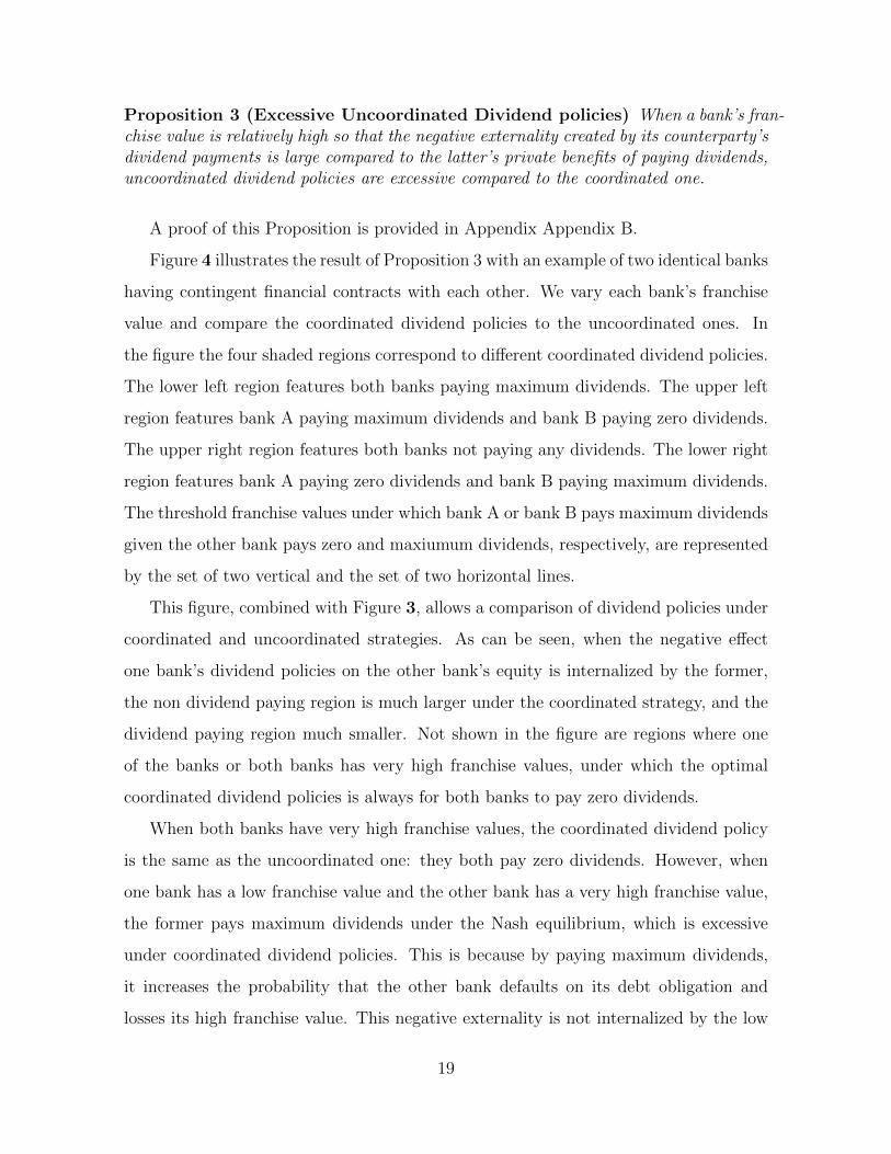
Proposition 3 (Excessive Uncoordinated Dividend policies) When a bank’s fran-chise value is relatively high so that the negative externality created by its counterparty’sdividend payments is large compared to the latter’s private benefits of paying dividends,uncoordinated dividend policies are excessive compared to the coordinated one.

A proof of this Proposition is provided in Appendix Appendix B.

Figure 4 illustrates the result of Proposition 3 with an example of two identical banks

having contingent financial contracts with each other. We vary each bank’s franchise

value and compare the coordinated dividend policies to the uncoordinated ones. In

the figure the four shaded regions correspond to different coordinated dividend policies.

The lower left region features both banks paying maximum dividends. The upper left

region features bank A paying maximum dividends and bank B paying zero dividends.

The upper right region features both banks not paying any dividends. The lower right

region features bank A paying zero dividends and bank B paying maximum dividends.

The threshold franchise values under which bank A or bank B pays maximum dividends

given the other bank pays zero and maxiumum dividends, respectively, are represented

by the set of two vertical and the set of two horizontal lines.

This figure, combined with Figure 3, allows a comparison of dividend policies under

coordinated and uncoordinated strategies. As can be seen, when the negative effect

one bank’s dividend policies on the other bank’s equity is internalized by the former,

the non dividend paying region is much larger under the coordinated strategy, and the

dividend paying region much smaller. Not shown in the figure are regions where one

of the banks or both banks has very high franchise values, under which the optimal

coordinated dividend policies is always for both banks to pay zero dividends.

When both banks have very high franchise values, the coordinated dividend policy

is the same as the uncoordinated one: they both pay zero dividends. However, when

one bank has a low franchise value and the other bank has a very high franchise value,

the former pays maximum dividends under the Nash equilibrium, which is excessive

under coordinated dividend policies. This is because by paying maximum dividends,

it increases the probability that the other bank defaults on its debt obligation and

losses its high franchise value. This negative externality is not internalized by the low

19

franchise bank under uncoordinated dividend policies.

4.2 Global Game Refinement

Having identified the multiplicity of equilibria of the 2 × 2 game due to the payoff

spillovers of bank dividends, we now employ global game techniques to refine the out-

come. Following the constructions used in the global game literature (Morris and Shin

(1998, 2001, 2003)), we consider the following variation of our model.

First, the game is symmetric in the sense that all parameters are identical across the

two banks. Hence, if the franchise values of the two banks are identical Va = Vb = V ,

the promised payoffs under the OTC contracts are identical, so that sa = sb = s, and

both banks have the same cash holding ca = cb = c.

However, rather than being a parameter that is common knowledge between the

banks, we suppose that V is uniformly distributed on the interval[0, V

]where V is

large relative to the threshold points V ∗a and V ∗b for the two banks.

Second, rather than the franchise values of the two banks being common knowledge,

assume that each bank observes a slightly noisy signal of the common franchise value.

Specifically, bank A observes the realization of the signal xa given by

xa = V + εa (27)

where εa is a uniformly distributed noise term, taking values in [−η, η] for small η > 0.

Similarly, bank B observes signal xb = V + εb where εb is uniformly distributed in

[−η, η]. We assume that the realizations of εa, εb and V are all mutually independent.

The noisy nature of the signals defines a Bayesian game built around the underlying

one shot game, called the global game (see Morris and Shin (1998) for details). The

strategy of a bank maps each realization of its signal xi to its dividend payment di ∈

{0, ci}. An equilibrium is defined as a pair of strategies where the action prescribed

given signal realization xi maximizes bank i’s expected payoff conditional on its signal

realization given the opponent’s strategy.

20

A switching strategy associated with a switching point x∗ is defined as the mapping:

d (xa) =

0 if xa ≥ x∗

ca if xa < x∗(28)

We then have the following result for the global game refinement of our dividend

game. Define the function W (x) as

W (x) ≡ 12W (0, x) + 1

2W (c, x) (29)

where W (db, x) is the function defined in (19) that gives the payoff advantage to bank

A with franchise value V = x of paying zero dividends over paying maximum dividends

when bank B pays dividends of db. The function W (x) defined above has the inter-

pretation of the expected payoff advantage to bank A of paying zero dividends when

bank B is randomizing equally between paying zero dividends and paying maximum

dividends. Given the symmetry of the payoff parameters, W (x) also applies to bank

B’s payoff advantage given bank A’s dividend policy.

With these preliminary definitions, we have our main result on the global game

refinement of equilibrium.

Proposition 4 (Global Game Refinment) There is a unique x∗ that solves W (x∗) =0. There is an equilibrium of the global game where both banks use the switching strategyaround the switchng point x∗. There is no other equilibrium in switching strategies.

The proof of this Proposition follows in three steps. First, we know from the

expression (21) that both W (0, x) and W (c, x) are increasing linear functions of x

with slope c/(y − y

), so that W (x) is also an increasing linear functions of x with

slope c/(y − y

). Since W (x) changes sign from negative to positive as x increases,

there is a unique x∗ that solves W (x∗) = 0.

Next, we show that both banks using the switching strategy around x∗ constitutes

an equilibrium of the global game. Conditional on bank A observing the signal xa = x,

the expected payoff advantage of paying zero dividends over paying maximum dividends

is given by

Pr (db = 0|xa = x)×W (0, x) + Pr (db = c|xa = x)×W (c, x) (30)

21

Suppose that both banks employ the switching strategy around the point x∗ where x∗

solves W (x∗) = 0. Then, we have

Pr (db = 0|xa = x∗) = Pr (xb > x∗|xa = x∗)

Pr (db = c|xa = x∗) = Pr (xb ≤ x∗|xa = x∗)

Given the symmetric nature of the noisy signals of the two banks, we have

Pr (xb > x∗|xa = x∗) = Pr (xb ≤ x∗|xa = x∗) =1

2(31)

Thus, conditional on bank A observing the signal xa = x, the expected payoff advantage

of paying zero dividends over paying maximum dividends is given by

12W (0, x∗) + 1

2W (c, x∗) = 0

so that bank A is indifferent between paying zero dividends and maximum dividends.

For signal x > x∗, Pr (db = 0|xa = x) > 12, so that bank A strictly prefers to pay zero

dividends. Analogously, for signal x < x∗, Pr (db = 0|xa = x) < 12, so that bank A

strictly prefers to pay maximum dividends of c. Hence, the switching strategy around

x∗ is the best response of bank A when bank B itself follows the switching strategy

around x∗. Given the symmetric nature of the game, an exactly analogous argument

shows that the switching strategy around x∗ by bank B is the best response when bank

A uses the same strategy. This proves that the strategy pair where both banks use

switching strategies around x∗ is an equilibrium of the global game.

The final part of the proposition claims that there is no other switching equilibrium

of the global game. But this claim is immediate from the fact that x∗ is the unique

solution to W (x) = 0. If, contrary to the Proposition there is another switching

equilibrium around the point x′, where x′ 6= x∗, then we have W (x′) 6= 0 so that the

switching strategy around x′ cannot be the best response to the switching strategy

around x′ by the other bank. This completes the proof of the proposition.

The global game refinement is preserved in the limiting case where the noisy signal

becomes increasingly accurate, since the key feature of the construction is to maintain

the joint density of the signal realizations that bank A’s signal is equally likely to be

22

higher or lower than the realization of bank B’s signal. This feature of the joint

signal realizations does not depend on the support [−η, η] of the noise in the banks’s

signal. Even in the limit as η → 0, we have the key feature that Pr (xb > x∗|xa = x∗) =

Pr (xb ≤ x∗|xa = x∗) = 12.

5 Risk-Shifting in Equilibrium

Having verified that global game techniques can be applied to refine the equilibrium,

we revert back to the more general payoffs for the two banks and address the question

of why risk-shifting via dividends can happen in equilibrium, given that the costs of

risk-shifting to creditors should be fairly priced in ex-ante contracts. What if banks

pre-commit to a lower probability of risk-shifting through raising less debt? In this

section, we argue that when banks have high expected franchise values at t = −1

that are significantly eroded at t = 0, risk-shifting can happen ex-post even with such

pre-commitment.

To understand this argument, we revert to the single bank setting and analyze the

optimal leverage decision of the bank at time t = −1. To fund an investment that

costs I, the bank chooses to raise D(`) in debt and I − D(`) in equity, where D(`)

denotes the price of debt with face value ` due at t = 1. The bank’s franchise value

is distributed over some random distribution function at t = −1 and is only realized

at t = 0. Assume again that there is no discounting for the time value of money. The

price of debt with a face value of ` is given by:

D (`) =

∫ y

y

`h (y) dy +

∫ y

y

yh (y) dy

where the first term is the expected value of debt that is fully recoverable in no default

states; and the second is the expected cash flow creditors can recover in default states.

Given this price of debt, the rate of return required by debt holders, or in other words

the cost of debt at t = 0 is:

23

rD ≡`

D (`)− 1

We have that:

∂rD∂`

=2(y2 − y2 + 2` (`− y)

) (y − y

)(2` (y − y) + y2 − y2

)2 > 0

and that:∂rD∂d

=2` (`− y)

(y − y

)(2` (y − y) + y2 − y2

)2 > 0

As can be seen, the cost of debt is increasing in both (i) leverage and (ii) dividends.

(i) reflects the higher credit risk associated with a reduced ability to service a higher

amount of debt in the bad states. (ii) reflects the cost of risk-shifting via the payout

policy. We know from before that banks either pay maximum or zero dividends, and

that the probability of paying maximum dividends increases in leverage. This allows

us to characterize the cost of debt for different levels of leverage, taking into account

the endogenous dividend decision. A bank is expected to pay maximum dividends at

t = 0 if leverage exceeds a threshold `∗∗, given by the following expression:

`∗∗ =2y + c+ 2E (V )

2

The relation between the cost of debt and leverage can be best illustrated with an

example. Figure 5 plots the t = −1 cost of debt for a bank with c = 100, y = 0, y = 300,

and E (V ) = 200 against the bank’s leverage `. The cost of debt is calculated as `D(`)−1.

The solid line represents the cost of debt attributable to credit risk, assuming that the

bank does not pay any dividends for all levels of leverage. The dashed line represents

the cost of debt attributable to both credit risk and agency costs, if any, created by the

bank’s optimal dividend policy. `∗∗ is the critical value of leverage above which the bank

is expected to pay maximum dividend, and below which no dividends. When leverage

is below the critical threshold `∗∗, the bank is expected not to pay any dividends, and

the cost of debt only reflects its credit risk. When leverage is past the critical value `∗∗,

however, the bank is expected to risk-shift by paying maximum dividends. In this case,

the cost of debt is now higher, reflecting the added agency problem of risk shifting.

24

The bank will choose the optimal debt-equity mix where the marginal cost of debt

equals its marginal benefits. The benefits of debt can be substantial, for the following

reasons. First, because equity is more informationally sensitive than debt, and more

so for such institutions with opaque assets such as banks, issuing more debt enables

banks to save on the equity issuance costs. Myers and Majluf (1984) suggest that

because managers have private information about future prospects of the firm, outsiders

believe that a bank will only issue informationally sensitive equity if it is overvalued.

As a result, equity issuance entails a drop in the bank’s stock price as the market

incorporates its belief. This result has been empirically documented in Masulis and

Konwar (1986), Asquith and Mullins (1986), to name just a few. Second, as with other

forms of corporations, interest paid on debt is tax deductible, making debt an attractive

financing instrument. Absent the agency costs of risk-shifting, we assume an extreme

case in which the benefits of debt exceed its costs attributable to default at all levels of

leverage, and hence banks would like to take on as much debt as possible.2

If the agency cost of debt is not very high, the benefits of debt dominate and the

bank will choose maximum leverage and bear the potential agency costs of risk-shifting.

In this case, any risk-shifting that happens at t = 0 is an expected outcome that is fairly

priced in debt contracts. If the agency cost of debt is high enough, however, the bank

may choose to pre commit at t = −1 by choosing a leverage level immediately to the

left of `∗∗. At time t = 0, if the franchise value gets a significant negative shock such

that E (V ) > V , the ex-post threshold leverage above which agency costs kicks in can

be much lower than `∗∗ and the bank risk-shifts. This explains why high leverage can

be the optimal solution ex-ante, but may become overly excessive (from the standpoint

of creditors) ex-post.3

Note that we have not solved formally for the optimal leverage decision at time

t = −1, which is beyond the scope of this paper. The purpose of this section is to show

2This corresponds to the usual argument from bankers that equity is much more expensive thandebt, and the empirical observation that banks have high leverage.

3The main conclusion does not change if we assume that optimal debt absent agency costs of risk-shifting is an intermediate value. Here, even when the bank is not in the risk-shifting region ex-antefor the purpose of debt pricing, the probability of ex-post risk-shifting will be positively related to thesize of the negative shock to the bank’s franchise value.

25

that even if the expected agency cost of risk-shifting via dividends is fairly priced ex-

ante, ex-post risk-shifting may exist in equilibrium as a bad outcome for creditors. The

bank can pre-commit not to pay dividends by raising less leverage and thus avoiding

this cost, yet a sufficiently bad shock to its franchise value ex-post may make it optimal

for the bank to abandon such a commitment.

6 Relaxing Model Assumptions

In this section, we discuss the implications from relaxing several assumptions we made

in our benchmark model.

6.1 Seniority of Bank Debt

So far in our two-bank model, we have assumed that bank debt is of the same seniority

as all other nonbank debt. While this assumption is not responsible for any qualitative

results we obtained, we now discuss the implication of relaxing this assumption and

making bank debt senior to all nonbank claims in a financial firm’s capital structure.

This is in line with the practical observation that bank debt is usually secured by

collateral (Welch, 1997) and represents the first claims on the failed firms’ assets. We

argue that bank debt seniority makes it less likely for the bank to risk-shift: the bank’s

threshold franchise value, under which it pays maximum dividend, is smaller when

bank debt is more senior. Intuitively, when bank A’s debt is senior, the amount of cash

bank A expects to receive from bank B in debt settlements is higher than that in the

benchmark case. This reduces bank A’s leverage compared to the benchmark case’s

level, lowering the probability bank A will risk-shift. In addition, negative externalities

imposed on bank A from bank B’s dividend payments are not as big as in the case where

all debt claims are of equal seniority. This is because the probability of B defaulting

on A is now lower; moreover, the amount A is able to recover from B, upon the latter

defaulting, is now higher.

26

6.2 Correlated Cash Flows

We now relax the assumption that cash flows of banks A and B are uncorrelated. Recall

that a loss in bank A’s value attributable to B’s dividend payment can be broken down

into two components. The first component relates to an increase in the expected loss

of bank A’s franchise value as a result of increased default probability. The second

component arises from the fact that A is unable to recover full payment from B in B’s

default state. Note that this value loss to equityholders only happens in A’s solvency

states (In A’s default states, A’s equity value does not depend on whether full payment

is recovered from B). While relaxing the assumption of independent cash flows does

not affect the first component, it does affect the second component. If banks’ cash

flows are positively correlated, B’s default states are likely to happen at the same time

with A’s default states, and therefore negative externalities are lower compared to the

benchmark result. By similar reasoning, dividend externalities are greater than the

benchmark result when cash flows are negatively correlated.

6.3 Correlation between Cash Flows and States Driving In-terdependence

We now discuss implications from relaxing the assumption that cash flows and states

driving interdependence via contingent financial contracts are uncorrelated. It is easy

to see that the expected magnitude of the negative externalities that B imposes on A

by paying dividends, measured by A’s expected loss from less than full payment from

B in B’s default states, is decreasing in the correlation between B’s cash flows and

the probability that B has to make payments to A. When this correlation is negative,

that is, when bank B is more likely to owe sb to bank A in B’s low cash flow states,

B will find itself more often unable to make full payments to bank A when state B

arises, thereby imposing a more significant negative externality on A’s equity value.

On the other hand, when the correlation is positive, bank B is more likely to make full

payments to A when state B occurs, lowering the negative externalities imposed on A

by B’s dividend policy.

27

7 Discussion and Policy Implications

7.1 Relationship to Dividend Payouts During 2007-2009

Our result is helpful in understanding the divergent dividend patterns documented in

section 2. All the financial firms mentioned had very high leverage ratios coming into

the crisis. This, coupled with the fact that current and expected future cash flows were

low means that these firms, according to the model, had substantial benefits from risk-

shifting via a maximum dividend policy. In fact, consistent with the model’s result that

the probability of dividend payment is increasing in leverage, Lehman Brothers, being

the most highly levered bank, increased its dividends remarkably in the period leading

up to its failure. On the other hand, commercial banks, which were not as highly

levered as securities firms due to their tighter capital requirements, either smoothed

out or decreased their dividends throughout the crisis.

High leverage, however, should not result in risk-shifting if the franchise value of the

bank is high enough. According to our model, the bank tends to risk-shift by paying

dividends only when a bad shock depresses a bank’s franchise value to a sufficiently low

level. While banks’ franchise values were depressed during the crisis, there are reasons

to believe that they were more depressed for securities firms compared to commercial

banks, resulting in the observed dividend behavior. While commercial banks’ clients,

whose relationship with the bank are commonly formed through illiquid loan contracts,

are not very likely to fly during bad times, securities firms’ customers may have found

it easier to exit relationships.

In fact, the crisis of 2007-2009 revealed that a major class of securities firms’ clients

- hedge funds relying on prime brokerage services- are prepared to shift their cash and

securities to safer institutions when signs of distress occur. The collapse of Bear Stearns

and Lehman Brothers prompted large flows of hedge fund client assets out of Morgan

Stanley and Goldman Sachs (those with historically the largest share of the prime

brokerage business), and into commercial banks that were perceived, at the time, as

28

the most creditworthy, such as Credit Suisse, JP Morgan, and Deutsche Bank.4 Since

prime brokerage is a high profit margin activity, that involves the bank lending cash

and securities to hedge funds and providing custody and other businesses, the loss of

relationships with hedge fund clients may have caused a significant decline in franchise

values of many securities firms and potentially an increase in franchise values of several

creditworthy commercial banks.

A potential alternative explanation for the divergence in dividend behavior is the

presence of the Prompt Corrective Action (PCA) procedure that applies only to insured

depository institutions (Section 38 of the Federal Deposit Insurance Act). This pro-

cedure requires such institutions and the federal banking regulators to resolve capital

deficiencies via prompt corrective actions, which, among other things, include a suspen-

sion of dividends by undercapitalized depository institutions. A depository institution

is undercapitalised for PCA purposes if either of the following happens: 1. Total risk

based capital ratio falls below 8%; 2. Tier 1 capital ratio falls below 4%; and 3. Lever-

age capital falls below 4%. If losses during 2007-2008 had made Washington Mutual

and Wachovia undercapitalized or more likely to be undercapitalised, their dividend

cuts would have been consistent with PCA. Lehman Brothers and Merrill Lynch, on

the other hand, were not subject to PCA and hence would have seen their risk-shifting

materialized, as our model predicts.

Anecdotal evidence indeed suggests PCA might have been more effective than mar-

ket pressure in limiting risk-shifting behavior. Wachovia and Washington Mutual were

among the banks that slashed dividends and raise additional capital in 2008 in order

to preserve capital under regulatory pressure, due to heavy subprime related losses.

Wachovia was not adequately capitalised for PCA purposes throughout 2007 and 2008,

when its risk based capital ratio was consistently below 8%.5 In a report on Wa-

chovia issued on July 22, 2008, the Federal Reserve acknowledged Wachovia’s capital

4According to Global Custodian magazine, 44 percent of hedge funds reduced balances with Gold-man and 70 percent backed out from Morgan Stanley.

5Wachovia’s risk based capital ratios were 0.0729 for Q1, 2007, 0.0735 for Q2, 2007, 0.071 for Q3,2007, 0.0751 for Q4, 2007, 0.0751 for Q1, 2008, 0.0726 for Q2, 2008, 0.0731 for Q3, 2008. These ratiosare collected from Compustat.

29

restoration efforts via cutting dividends, issuing equity and adopting strategies to limit

asset growth. However, it also expected “management to consider additional actions

including further reducing its dividend and/or raising additional capital to ensure that

corporation maintains sufficient capital”.

Washington Mutual, on the other hand, was well capitalised throughout the period

examined. Nonetheless, for Q4, 2007, the firm took its first loss in 10 years with $3

billion in write-downs due to mortgage and loan losses. Increasing losses led to the

significant drop in its total risk based capital ratio from 12.21% in Q1, 2008 to 8.4%

in Q2, 2008, putting pressure on the bank to restore its capital. Wamu’s chairman and

CEO, Kerry K. Killinger, said in a statement that dividend cuts and equity issues in

2008 were actions that “aimed to fortify WaMu’s strong capital and liquidity position”.

While investment banks do not face any regulatory pressure with regard to capital

preservation, market perception is that capital depletion would likely hurt their future

growth prospects. Yet even when the bank’s asset values declined and subprime losses

consumed its capital and threatened its survival, Lehman kept paying dividends and

repurchasing stock. In an October 6, 2008 hearing, Henry Waxman, chairman of the

oversight and government reform committee, called the payout actions of Lehman’s

CEO, Dick Fuld, “questionable”, stating: “In a January 2008 presentation, he and the

Lehman board were warned that the company’s “liquidity can disappear quite fast.”

Yet despite this warning, Mr. Fuld depleted Lehman’s capital reserves by over $10

billion through year-end bonuses, stock buybacks, and dividend payments”. Similarly,

Merrill Lynch kept increasing dividends, despite mounting concern among investors

and analysts. According to analyst Brad Hintz of Sanford C. Bernstein, “the high

dividend payout ratio will place constraints on the company’s inventory and balance

sheet capacity, and limit its ability to compete effectively in fixed-income proprietary

trading” (Dealbook article, August 6, 2008).6

6http://dealbook.nytimes.com/2008/08/06/merrill-should-cut-dividend-analyst-says/.

30

7.2 Policy Implications

Our model provides theoretical rationale for the use of dividend restrictions as part

of the U.S Prompt Corrective Action (PCA) procedure. Introduced in 1991 following

the banking crisis in the 1980’s, PCA was an early intervention mechanism intended to

provide swift measures to turn around troubled financial institutions. Among different

measures are mandatory limits to dividends and compensation to senior managers of

banks that are under-capitalized.7

Our model confirms the relevance of PCA in crisis periods when banks usually find

their franchise values depressed and themselves pushed into the risk-shifting/ dividend

paying regions. Risk-shifting by individual banks, however, is not sufficient for dividend

restrictions to be necessary. These restrictions are only useful if the economy embodies

many interconnected banks (which indeed is the case for the US financial market) of

both high and low franchise values where dividend policies are negative externalities

to the value of each other. As we have shown, limiting dividend payments, a measure

analogous to what we called a coordinated dividend policy, can help preserve bank

capital in a socially optimal way.

Along the same lines, our model supports the Basel III accord which established that

banks must maintain a capital conservation buffer consisting solely of Tier I capital and

accounting for 2.5% of the banks’ risk-weighted assets. Building this buffer may involve

reductions in discretionary earnings distribution, dividend payments, and salaries and

bonuses. Basel III also suggests that regulators forbid banks from distributing capital

when banks have depleted their capital buffers.

In this regard, the policy implications of our paper is in line with those from Ad-

mati et al. (2011) and Acharya, Mehran and Thakor (2012), which advocate dividend

restrictions and capital conservation in bad times. Admati et al. (2011) argue that

bank equity can provide significant social benefits. Specifically, they argue that higher

capital means that equity holders and bank managers have more “skin in the game”

7Compensation to senior managers of banks can be thought of as dividends paid to internal capital,and hence is applicable to our model here.

31

and thereby are less inclined to take excessive risk. This rationale is consistent with

our first theoretical result that banks’ incentives to transfer value away from creditors

to shareholders, in particular, by paying out dividends, increase with leverage.

Analyzing the payout decision from a different angle, Acharya, Mehran and Thakor

(2012) reach the same conclusion as ours that part of bank capital should only be

available to equity holders when banks perform well. Acharya, Mehran and Thakor

(2012) argue that banks tend to fund themselves with excessive leverage in anticipation

of correlated failures and government bail-out of bank creditors. Consequently, optimal

regulation features a contingent rule, in which part of bank capital is unavailable to

creditors upon failure and available to shareholders only in the good states.

While the recommendations for dividend restriction by Admati et al. (2011) and

Acharya, Mehran and Thakor (2012) are based on a moral hazard argument as in our

paper, the novel element central to our analysis is the presence of bank interconnect-

edness and dividend externalities. In our model, dividend restriction arises not from

the desire to curb an agency problem (excessive risk taking) between shareholders and

creditors of individual banks, but from a failure to coordinate among shareholders of

interconnected banks. Without such coordination, individual banks do not internalize

the negative externalities they impose on their interconnected banks, and hence their

dividend payout might be excessive relative to a socially optimal outcome.

Our model also speaks for the social benefits of clearing-house arrangements. Under

these arrangements, banks internalize costs of their default on each other by all putting

upfront margins and capital. Ex-post, when one is in trouble, this upfront capital can

be used for co-insurance. Dividend policy can be understood in light of this general

principle. Originally, clearinghouses of commercial banks were formed mainly to deal

with information based contagion. Clearinghouses for derivatives, on the other hand,

are intended to deal with counterparty risk and interconnectedness issues (Duffie and

Zhu, 2011). The key insight is that in each of these cases, one bank’s equity is effectively

- and in part - a debt claim on other banks. Hence, insights from agency problems

between equity and debt of each bank carry over to conflicts of interest across inter-

32

connected banks.

8 Conclusion

Why did banks continue to pay dividends well into the 2007-2009 financial crisis? We

argue in this paper that a combination of risk-shifting incentives and low franchise

values can lead to such a striking dividend pattern. Interestingly, when banks are

contingent creditors of each other, dividend payouts by one bank may exert negative

externalities on the other banks’ equity. Because individual banks do not internalize

these negative externalities, their non-coordinating dividend policies can be excessive,

e.g. in cases where the franchise values of some of these banks are not too low.

Our model generates two main testable hypotheses as follows. First, during financial

crises, banks that have higher leverage or lower franchise values are more likely to

risk-shift via dividend payments. Second, banks that are more connected with each

other have dividend policies that are more likely to exhibit strategic complementarities.

Although the first hypothesis has been discussed under previous models, we believe

that the second hypothesis is novel.

Our arguments call for policy measures in coordinating dividend payments during

bad times, where continuation values of some banks can be sufficiently low and risk

taking incentives via dividend payments can be substantial. If low franchise value

banks can agree not to pay dividends, the franchise values of its counterparty banks are

less likely to be lost, capital is better preserved, and as a consequence the total value

of the financial sector could be higher.

References

Acharya, Viral V., Hamid Mehran, and Anjan Thakor, 2010, “Caught Between Scylla

and Charybdis? Regulating Bank Leverage When There is Rent Seeking and Risk

Taking”, Working paper, NYU-Stern, New York Fed, and Washington University

at St. Louis.

33

Acharya, Viral V., Sergei Davydenko and Ilya Strebulaev, 2012, “Cash Holdings and

Credit Risk”, Review of Financial Studies, Vol. 25 (12), pp. 3572-3609.

Acharya, Viral V., Irvind Gujral, Nirupama Kulkarni, and Hyun S. Shin, 2011, “Div-

idends and Bank Capital in the Financial Crisis of 2007-2009”, Working paper,

NYU-Stern and Princeton University.

Admati, A., Peter M. DeMarzo, Martin F. Hellwig, and Paul Pfleiderer, 2011, “Falla-

cies, Irrelevant Facts, and Myths in the Discussion of Capital Regulation: Why

Bank Equity is Not Expensive”, Working Paper, Stanford GSB.

Aggarwal, R. and K. T. Jaques, 2001, “The Impact of FDICIA and prompt corrective

action on bank capital and risk: Estimates using a simultaneous equations model”,

Journal of Banking and Finance, Vol. 25, 1139-1160.

Asquith, P. and Mullins, D., 1986, “Equity Issues and the Offering Dilution”, Journal

of Financial Economics, Vol. 15 (1,2), pp. 61-89.

Benston, J. G. and G. J. Kaufman, 1997, “FDICIA after Five Years”, Journal of

Economic Perspectives 11, 139-158.

Duffie, D., and Haoxiang Zhu, 2011, “Does a Central Clearing Counterparty Reduce

Counterparty Risk?”, Review of Asset Pricing Studies, Vol. 1(1), pp. 74-95.

Esty, Benjamin C., 1997, “Organizational Form and Risk Taking in the Savings and

Loan Industry”, Journal of Financial Economics, Vol. 44, pp. 22-55.

Freixas, Xavier, and Bruno M. Parigi, 2008, “Banking Regulation and Prompt Cor-

rective Action”, CESifo Working Paper Series No. 2136.

Freixas, Xavier, Jean-Charles Rochet, and Bruno M. Parigi, 2010, “The Lender of Last

Resort: A Twenty-First Century Approach”, Journal of the European Economic

Association, Vol. 2(6), pp. 1085-1115.

34

Galai, D. and R. Masulis, 1976, “The Option Pricing Model and The Risk Factor of

Stock”, Journal of Financial Economics, Vol. 3, pp. 53-81.

Helmann, T.F., K.C. Murdock, J.E. Stiglitz, 2000, “Liberalization, moral hazard in

banking, and prudential regulation: Are capital requirements enough?”, American

Economic Review, Vol. 80, 1183- 1200.

Jensen, M. C., and Meckling, W. H., 1976, “Theory of The Firm: Managerial Behavior,

Agency Costs and Ownership Structure”, Journal of Financial Economics, Vol.

3(4), pp. 305-360.

Masulis, R., and Konwar, A., 1986, “Seasoned Equity Offerings: An Empirical Inves-

tigation”, Journal of Financial Economics, Vol 15 (1,2), pp. 91-118.

Morris, Stephen and Hyun Song Shin (1998),“Unique Equilibrium in a Model of Self-

Fulfilling Currency Attacks”, American Economic Review, Vol. 88, pp. 587-597.

Morris, Stephen and Hyun Song Shin (2001) “Rethinking Multiple Equilibria in Macroe-

conomic Modelling”, NBER 2000 Macroeconomics Annual, MIT Press, 2001.

Morris, Stephen and Hyun Song Shin (2003) “Global Games: Theory and Applica-

tions” in Advances in Economics and Econometrics, the Eighth World Congress

(edited by M. Dewatripont, L. Hansen and S. Turnovsky), Cambridge University

Press, 2003.

Myers, S. (1977), “Determinants of Corporate Borrowing”, Journal of Financial Eco-

nomics, Vol. 5(2), pp. 147-175.

Myers, S., and Majluf, N., 1984, “ Corporate Financing and Investment Decisions

when Firms Have Information That Investors Do Not Have”, Journal of Financial

Economics, Vol. 13 (2), pp. 187-221.

Saunders, Anthony, Elizabeth Strock, and Nickolaos G. Travlos, 1990, “ Ownership

Structure, Deregulation, and Bank Risk Taking”, Journal of Finance, Vol. 45 (2),

pp. 643-654.

35

Welch, I, 1997, “ Why is Bank Debt senior? A Theory of Asymmetry And Claim

Priority Based on Influence Costs”, Review of Financial Studies, Vol. 10(4), pp.

1203-1236.

36

Figure 1a: Cumulative Losses, 2007Q3 - 2008Q4

This figure plots the cumulative losses for the ten banks included in our study, over the periodfrom Quarter 3, 2007 to Quarter 4, 2008. All numbers are in billions of US dollars.

37

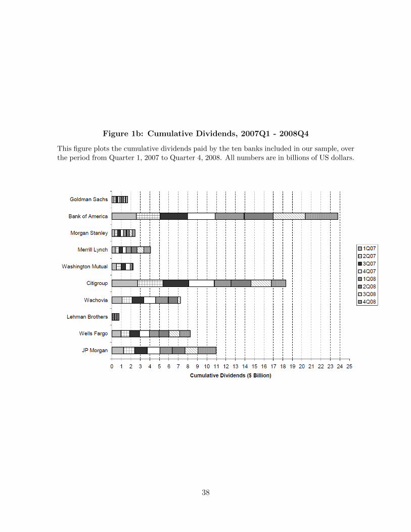
Figure 1b: Cumulative Dividends, 2007Q1 - 2008Q4

This figure plots the cumulative dividends paid by the ten banks included in our sample, overthe period from Quarter 1, 2007 to Quarter 4, 2008. All numbers are in billions of US dollars.

38

Figure 1c: Dividend Payments (2007Q1 = 1)

This figure plots dividend payments of the ten banks included in our sample, where all amountsare normalized so that the dividend payment in Quarter 1, 2007 is set to be equal to 1.

39

Figure 1d: Dividends as a Percentage of Book Equity (2007Q1 = 1)

This figure plots the ratio of dividends over book value of equity for the ten banks includedin our sample. All ratios are normalized such that the ratio in Quarter 1, 2007 is set equal to1.

40

Figure 2: Dividend Payments and Cumulative Losses

These figures plot cumulative losses alongside quarterly dividends for Lehman Brothers,Merrill Lynch, Washington Mutual, and Wachovia. All numbers are in billions of US dollars.

41

Figure 3: Strategic Complementarity of Dividend Policies

Va and Vb are the franchise values of banks A and B, respectively. V ∗i is the thresholdfranchise value of bank i (i ∈ {a, b}), below which it pays maximum dividends. di and ci are,respectively, the dividend payment and t = 1 cash flow of bank i. For each cell, the first andsecond values are the Nash dividend policy of bank A and bank B, respectively.

(ca, 0) (0, 0) (0, 0)

(ca, cb) (ca, cb) (0, 0)

(0, 0)

(ca, cb) (ca, cb) (0, cb)

Vb

Va

Va*

(db=0)

Vb*

(da=ca)

Vb*

(da=0)

Va*

(db=cb)

42

Figure 4: Excessiveness of Uncoordinated Dividend Policies

Va and Vb are the franchise values of banks A and B, respectively. The shaded regionscorrespond to different coordinated dividend policies. The lower left region features bothbanks paying maximum dividends. The upper left region features bank A paying maximumdividends and bank B paying zero dividends. The upper right region features both banksnot paying any dividends. The lower right region features bank A paying zero dividendsand bank B paying maximum dividends. Not shown in the plot are regions where oneof the banks or both banks has very high franchise values, under which the optimalcoordinated dividend policies is for both banks to pay zero dividends. The thresholdfranchise values under which bank A and B pays maximum dividends under the Nashequilibrium, respectively, are represented by the two vertical and the two horizontal lines.

43

Figure 5: Cost of Debt as A Function of Leverage

This figure plots the t = −1 cost of debt for a bank with c = 100, δmin = 0, δmax = 300, andE (V ) = 200 against the bank’s leverage l. Cost of debt is calculated as l

V (l)−1. The solid linerepresents the cost of debt attributable to credit risk, assuming that the bank does not payany dividends for all levels of leverage. The dashed line represents the cost of debt attributableto both credit risk and agency costs, if any, created by the bank’s optimal dividend policy. l∗∗

is the critical value of leverage above which the bank is expected to pay maximum dividends,and below which no dividends.

0

0.2

0.4

0.6

0.8

1

1.2

100 150 200 250 300

Co

st

of

deb

t

l

Cost of debt

attributable to credit

risk plus risk shifting

by dividends

Cost of debt

attributable to credit

riskl**

44

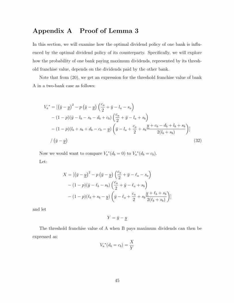
Appendix A Proof of Lemma 3

In this section, we will examine how the optimal dividend policy of one bank is influ-

enced by the optimal dividend policy of its counterparty. Specifically, we will explore

how the probability of one bank paying maximum dividends, represented by its thresh-

old franchise value, depends on the dividends paid by the other bank.

Note that from (20), we get an expression for the threshold franchise value of bank

A in a two-bank case as follows:

Va∗ = [

(y − y

)2 − p(y − y

) (ca2

+ y − la − sa)

− (1− p)(y − lb − sb − db + cb)(ca

2+ y − la + sb

)− (1− p)(lb + sb + db − cb − y)

(y − la +

ca2

+ sby + cb − db + lb + sb

2(lb + sb)

)]

/(y − y

)(32)

Now we would want to compare Va∗(db = 0) to Va

∗(db = cb).

Let:

X = [(y − y

)2 − p(y − y

) (ca2

+ y − `a − sa)

− (1− p)(y − `b − sb)(ca

2+ y − `a + sb

)− (1− p)(`b + sb − y)

(y − `a +

ca2

+ sby + `b + sb

2(`b + sb)

)]

and let

Y = y − y

The threshold franchise value of A when B pays maximum dividends can then be

expressed as:

Va∗(db = cb) =

X

Y

45

and the corresponding value for bank A when B pays zero dividends can be written as:

Va∗(db = 0) =

1

Y[X − (1− p) cbsb

2(`b + sb)(2(`b + sb − y)− cb)]

=1

Y[X − (1− p) cbsb

2(`b + sb)C]

where C = 2(`b + sb − y)− cbUsing the assumption that y < `i + si − ci < `i + si < y, we have that C > 0.

Therefore

Va∗(db = 0) < Va

∗(db = cb)

This result suggests that when two banks are interconnected (e.g., via a contingent

contract as described in our model), one bank is more likely to pay maximum div-

idends when the other bank pays maximum dividend. We call this result strategic

complementarity of dividend policies.

Appendix B Proof of Proposition 3

Excessive dividends can happen when either of the banks’ franchise value is sufficiently

low such that its optimal uncoordinated dividend policy is to pay maximum dividends.

Let d∗a and d∗b be the privately optimal (Nash) dividend policies for banks A and B,

respectively. Assume Va < V ∗a such that d∗a = ca. We will prove that when the fran-

chise value of B is big such that dividend externalities created by A’s dividends are too

large compared to its private gain, it is jointly optimal for bank A to pay less than its

privately optimal dividend level.

Assume now that bank A deviates from its privately optimal dividend policy and

pays da = d∗a − ε, while bank B employs its privately optimal policy db = d∗b . The

combined equity value of banks A and B in this case will be:

Ua(da, d∗b) + Ub(da, d

∗b)

The change in the combined bank value resulting from this deviation is:

46

Ua(da, d∗b) + Ub(da, d

∗b)− Ua(d

∗a, d∗b)− Ub(d

∗a, d∗b)

Let ε→ 0, we can write this expression as follows:

−∂Ua

∂dadda −

∂Ub

∂dadda = −

(∂Ua

∂da+∂Ub

∂da

)dda

where dda = ε. When d∗a = ca, we know from Proposition 3 that ∂Ua

∂da> 0. In addition,

∂Ub

∂dais always negative (Lemma 2). The former term represents the private benefits

of bank A from deviating while the latter represents the negative externalities A’s

dividends exert on B’s equity value. Let ∂f(Vb)∂Vb

≡ −∂Ub

∂da− ∂Ua

∂da, we have that

∂f(Vb)

∂Vb=p(`a + sa − y

)(y − y

)2 > 0

This makes intuitive sense. The higher B’s franchise value, the higher the magnitude

of the loss to the combined equity value resulting from negative externalities of A’

dividend payment, hence the higher the joint gain from A paying less than maximum

dividends. As the joint gain from bank A deviating is increasing in Vb, there exists a

sufficiently high value of Vb such that f(Vb) > 0, and A’s uncoordinated dividend policy

is jointly excessive.

Given the corner solution for the optimal dividend policy in our setup, bank A’s

dividend policy is jointly excessive if:

f ′ (Vb) ≡ − (Ub (da = ca)− Ub (da = 0))− (Ua (da = ca)− Ua (da = 0)) > 0

where

47

Ub (da = ca)− Ub (da = 0) =

−p ca(y − y

)2

((Vb − `b − db + cb + sa)

(y − `b − db + cb + sa) +y2 − (`b + db − cb − sb)2

2

)+

pca(y − y

)2

[y(Vb +

y

2

)− (Vb + y)

(`b + db − cb −

sa`a + sa

(ca2

+ y))

+0.5(

(`b + db − cb)2 +(`a + sa − ca − y

) sa`a + sa

(2 (`b + db − cb)−

saca`a + sa

)− sa

(`a + sa)

(sa

`a + sa

((`a + sa − ca)2 − y2

)− (`b + db − cb) (ca − 2 (`a + sa))

)+

s2a

3 (`a + sa)2

(3 (`a + sa)

2 − 3ca (`a + sa) + c2a

))]And Ua (da = ca)− Ua (da = 0) is given by:

Ua (da = ca)− Ua (da = 0) =ca

(y − y)2

[(y − y

)2 − p(y − y

) (Va +

ca2

+ y − la − sa)

−(1− p)(y − yb)(Va +

ca2

+ y − la + sb

)−(1− p)(yb − y)

(Va + y − la +

ca2

+ sby + cb − db + lb + sb

2(lb + sb)

)]As

∂f ′ (Vb)

Vb=pcasa

(2(`a + sa − y

)− ca

)2(y − y

)2(`a + sa)

> 0,

A’s uncoordinated dividend policy is excessive when Vb is sufficiently high, i.e., when

Vb >

(y − y

)2(2 (`a + sa))

pcasa(2(`a + sa − y

)− ca

) (γ + Ua (da = ca)− Ua (da = 0))

48

where

γ = −p ca(y − y

)2

((−`b − db + cb + sa)

(y − `b − db + cb + sa) +y2 − (`b + db − cb − sb)2

2

)+

pca(y − y

)2

[y( y

2

)− (y)

(`b + db − cb −

sa`a + sa

(ca2

+ y))

+0.5(

(`b + db − cb)2 +(`a + sa − ca − y

) sa`a + sa

(2 (`b + db − cb)−

saca`a + sa

)− sa

(`a + sa)

(sa

`a + sa

((`a + sa − ca)2 − y2

)− (`b + db − cb) (ca − 2 (`a + sa))

)+

s2a

3 (`a + sa)2

(3 (`a + sa)

2 − 3ca (`a + sa) + c2a

))]♦

49