basics in geostatistics geostatistical interpolation ... · pdf filebasics in geostatistics 2...

Basics in Geostatistics 2Geostatistical interpolation/estimation:

Kriging methods

Hans Wackernagel

MINES ParisTech

NERSC • April 2013

http://hans.wackernagel.free.fr

http://hans.wackernagel.free.fr

Basic concepts

Geostatistics

Hans Wackernagel (MINES ParisTech) Basics in Geostatistics 2 NERSC • April 2013 2 / 35

Concepts

Geostatistical model

The experimental variogram is used to analyzethe spatial structure of the data from aregionalized variable z(x).It is fitted with a nested variogram model, thusproviding the structure function of a randomfunction.The regionalized variable (reality) is viewed asone realization of the random function Z(x),which is a collection of random variables.

Kriging: a linear regression method for estimatingpoint values (or spatial averages) at any locationof a region.

Conditional simulation: simulation of an ensemble ofrealizations of a random function,conditional upon data — for non-linear estimation.

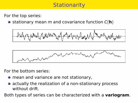
Stationarity

For the top series:

stationary mean m and covariance function C(h)

For the bottom series:

mean and variance are not stationary,

actually the realization of a non-stationary processwithout drift.

Both types of series can be characterized with a variogram.

Kriging of the mean

Kriging of the mean of a random function


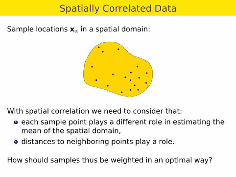
Spatially Correlated Data

Sample locations xα in a spatial domain:

●

●

●

●

●

●

●

●

●

●

●

●

●

●

●

●

●

●

With spatial correlation we need to consider that:

each sample point plays a different role in estimating themean of the spatial domain,

distances to neighboring points play a role.

How should samples thus be weighted in an optimal way?

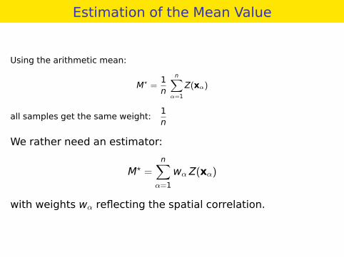
Estimation of the Mean Value

Using the arithmetic mean:

M? =1n

n∑α=1

Z(xα)

all samples get the same weight:1n

We rather need an estimator:

M? =n∑

α=1

wα Z(xα)

with weights wα reflecting the spatial correlation.

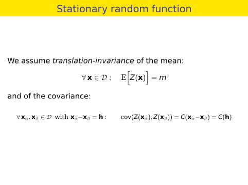
Stationary random function

We assume translation-invariance of the mean:

∀x ∈ D : E[Z(x)

]= m

and of the covariance:

∀xα,xβ ∈ D with xα−xβ = h : cov(Z(xα),Z(xβ)) = C(xα−xβ) = C(h)

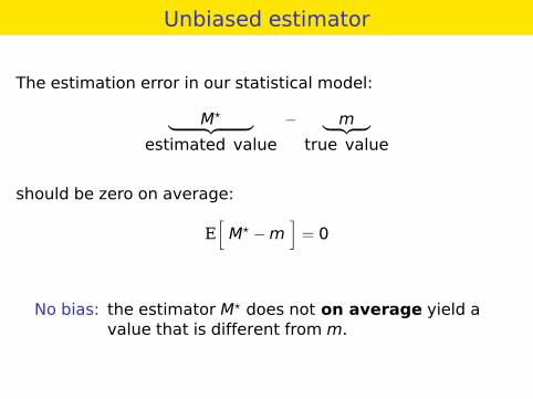
Unbiased estimator

The estimation error in our statistical model:

M?︸︷︷︸estimated value

− m︸︷︷︸true value

should be zero on average:

E[M? −m

]= 0

No bias: the estimator M? does not on average yield avalue that is different from m.

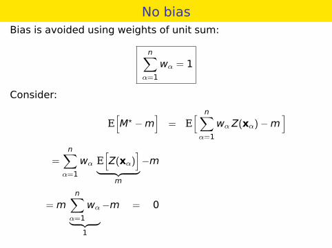
No biasBias is avoided using weights of unit sum:

n∑α=1

wα = 1

Consider:

E[M? −m

]= E

[ n∑α=1

wα Z(xα)−m]

=n∑

α=1

wα E[Z(xα)

]︸︷︷︸

m

−m

= mn∑

α=1

wα︸︷︷︸1

−m = 0

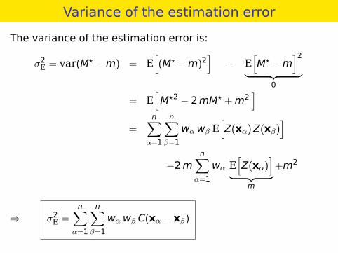
Variance of the estimation error

The variance of the estimation error is:

σ2E = var(M? −m) = E

[(M? −m)2

]− E

[M? −m

]2︸︷︷︸

0

= E[M?2 − 2mM? +m2

]=

n∑α=1

n∑β=1

wαwβ E[Z(xα)Z(xβ)

]

−2mn∑

α=1

wα E[Z(xα)

]︸︷︷︸

m

+m2

⇒ σ2E =

n∑α=1

n∑β=1

wαwβ C(xα − xβ)

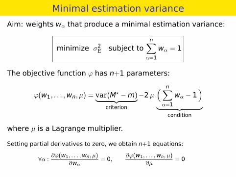
Minimal estimation variance

Aim: weights wα that produce a minimal estimation variance:

minimize σ2E subject to

n∑α=1

wα = 1

The objective function ϕ has n+1 parameters:

ϕ(w1, . . . ,wn, µ) = var(M? −m)︸︷︷︸criterion

−2µ( n∑α=1

wα − 1)

︸︷︷︸condition

where µ is a Lagrange multiplier.

Setting partial derivatives to zero, we obtain n+1 equations:

∀α :∂ϕ(w1, . . . ,wn, µ)

∂wα= 0,

∂ϕ(w1, . . . ,wn, µ)

∂µ= 0

Kriging equations

The method of Lagrange yields the equation system forthe optimal weights wKM

α of the estimation of the mean:

n∑β=1

wKMβ C(xα − xβ)− µKM = 0 for α = 1, . . . ,n

n∑β=1

wKMβ = 1

The variance at the minimum:

σ2KM = µKM

is equal to the Lagrange multiplier.

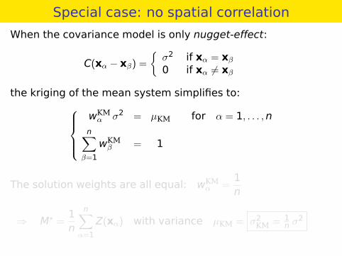
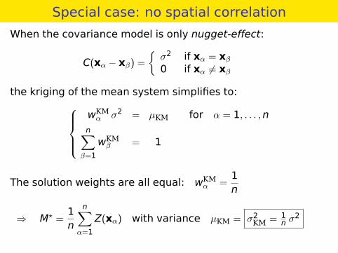
Special case: no spatial correlation

When the covariance model is only nugget-effect:

C(xα − xβ) ={σ2 if xα = xβ0 if xα 6= xβ

the kriging of the mean system simplifies to:wKMα σ2 = µKM for α = 1, . . . ,n

n∑β=1

wKMβ = 1

The solution weights are all equal: wKMα =

1n

⇒ M? =1n

n∑α=1

Z(xα) with variance µKM = σ2KM = 1

n σ2

Ordinary Kriging

Ordinary Kriging


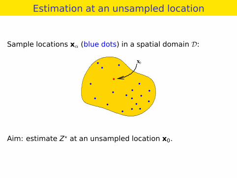
Estimation at an unsampled location

Sample locations xα (blue dots) in a spatial domain D:

●

●

●

●

●

●

●

●

●

●

●

●

●

●

●

●

x0

■

●

●

Aim: estimate Z? at an unsampled location x0.

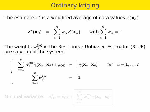
Ordinary kriging

The estimate Z? is a weighted average of data values Z(xα):

Z?(x0) =n∑

α=1

wα Z(xα) withn∑

α=1

wα = 1

The weights wOKα of the Best Linear Unbiased Estimator (BLUE)

are solution of the system:

n∑β=1

wOKβ γ(xα−xβ) + µOK = γ(xα−x0) for α = 1, . . . ,n

n∑β=1

wOKβ = 1

Minimal variance: σ2OK = µOK +

n∑α=1

wOKα γ(xα−x0)

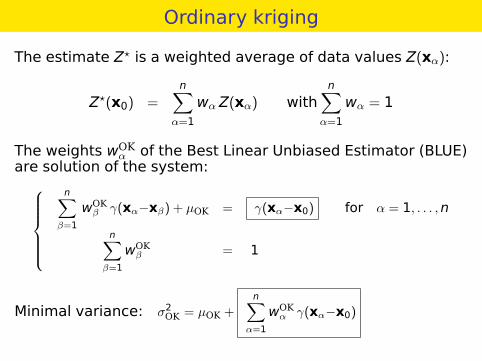
Kriging weights

The behavior of kriging weights


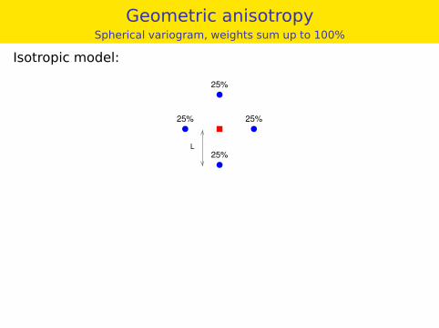
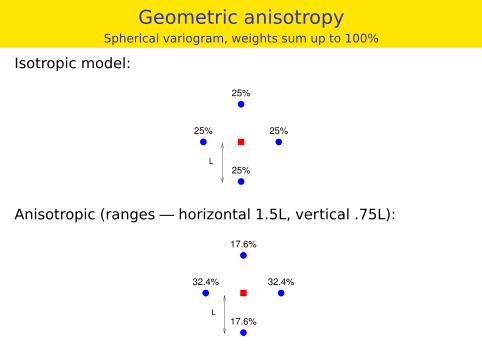
Geometric anisotropySpherical variogram, weights sum up to 100%

Isotropic model:

●

●

■ ●

L

25%

25%

25%

●

25%

Anisotropic (ranges — horizontal 1.5L, vertical .75L):

●

●

■ ●

L

17.6%

32.4%

17.6%

●

32.4%

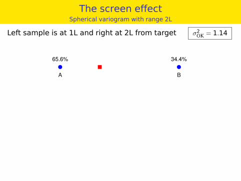
The screen effectSpherical variogram with range 2L

Left sample is at 1L and right at 2L from target σ2OK = 1.14

A B

● ■ ●

34.4%65.6%

Introducing an extra sample σ2OK = 0.87

A

● ■

49.1%

C

●

48.2%

B

●

2.7%

Adding the sample C screens off the sample B.

Case-study

Filtering noisy images by cokriging


Application: metallography

Trace elements are usually masked by instrumental noise.

Data: 512×512 image of phosphorus (P) trace elements.

Images for chrome (Cr) and (Ni) are less noisy.

Geostatistical filtering is used to remove the noise.

Structural analysis

Image of phosphorus Nested variogramγ(h) = 384 nug(h) + 75 exp(h) + 13 |h|

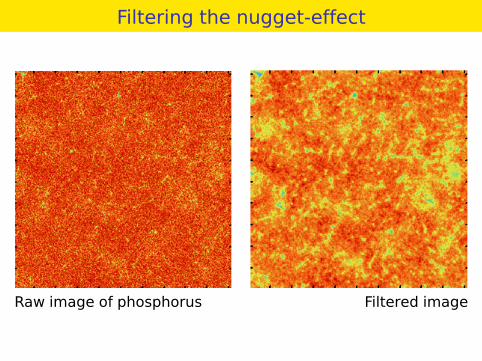
Filtering the nugget-effect

Raw image of phosphorus Filtered image

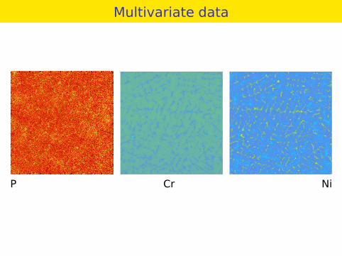
Multivariate data

P Cr Ni

Multivariate structural analysisDirect and cross variograms

Matrix variogram model: G(h) = B0 nug(h) + B1 exp(h) + B1 |h|

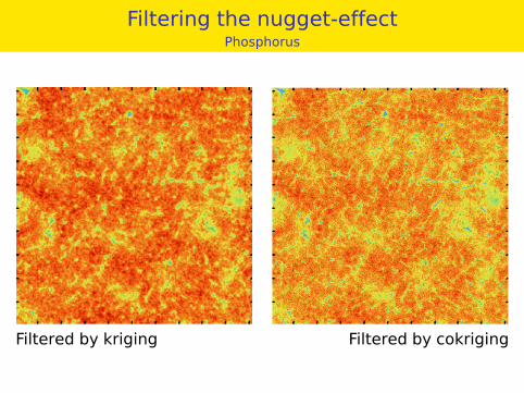
Filtering the nugget-effectPhosphorus

Filtered by kriging Filtered by cokriging

Case study

Space-time filteringSéguret & Huchon, JGR 1990


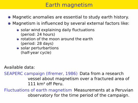
Earth magnetism

Magnetic anomalies are essential to study earth history.

Magnetism is influenced by several external factors like:

solar wind explaining daily fluctuations(period: 24 hours)rotation of the moon around the earth(period: 28 days)solar perturbartions(half-year cycle)

Available data:

SEAPERC campaign (Ifremer, 1986) Data from a researchvessel about magnetism over a fractured area of111 km² off Peru.

Fluctuations of earth magnetism Measurements at a Peruvianobservatory for the time period of the campaign.

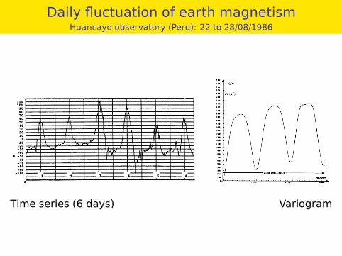
Daily fluctuation of earth magnetismHuancayo observatory (Peru): 22 to 28/08/1986

Time series (6 days) Variogram

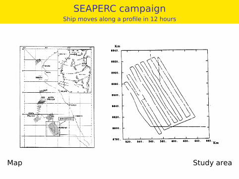
SEAPERC campaignShip moves along a profile in 12 hours

Map Study area

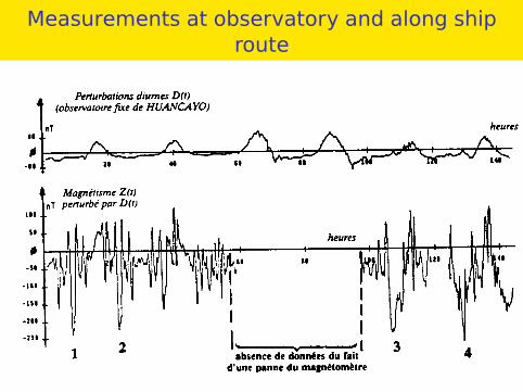
Measurements at observatory and along shiproute

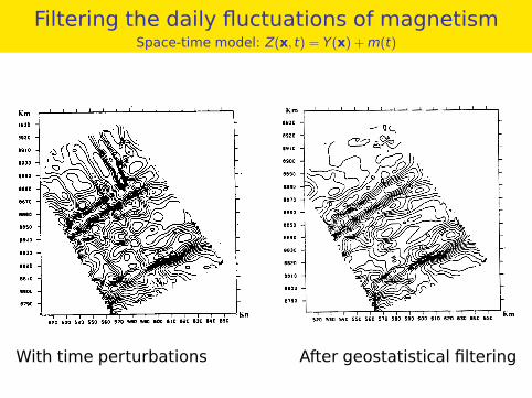
Filtering the daily fluctuations of magnetismSpace-time model: Z(x, t) = Y(x) +m(t)

With time perturbations After geostatistical filtering

Conclusion

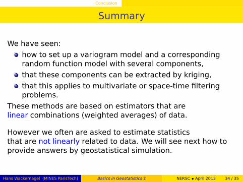
Summary

We have seen:

how to set up a variogram model and a correspondingrandom function model with several components,

that these components can be extracted by kriging,

that this applies to multivariate or space-time filteringproblems.

These methods are based on estimators that arelinear combinations (weighted averages) of data.

However we often are asked to estimate statisticsthat are not linearly related to data. We will see next how toprovide answers by geostatistical simulation.


References

JP Chilès and P Delfiner.Geostatistics: Modeling Spatial Uncertainty.Wiley, New York, 2nd edition, 2012.

G Matheron.The Theory of Regionalized Variables and its Applications.Number 5 in Les Cahiers du Centre de MorphologieMathématique. Ecole des Mines de Paris, Fontainebleau,1970.

S Séguret and P Huchon.Trigonometric kriging: a new method for removing thediurnal variation from geomagnetic data.J. Geophysical Research, 32(B13):21.383–21.397, 1990.

H Wackernagel.Multivariate Geostatistics: an Introduction withApplications.Springer-Verlag, Berlin, 3rd edition, 2003.

basics in geostatistics geostatistical interpolation ... · pdf filebasics in geostatistics 2...

Documents