before a board of inquiry tukituki catchment proposal · 1.4. i was maf’s national groundwater...

Before a Board of Inquiry

Tukituki Catchment Proposal

In the matter of the Resource Management Act 1991 (the Act)

AND

In the matter of a Board of Inquiry appointed under section 149J of the Act

to consider a plan change request, a notice of requirement

and applications for resource consents made by Hawkes Bay

Regional Council (HBRC) and Hawkes Bay Regional

Investment Company Ltd (HBRIC) in relation to the Tukituki

Catchment Proposal.

Statement of Evidence of Ian McIndoe for Ruataniwha Water Users Group (Groundwater Hydrology)

Dated 8 October 2013

BROOKFIELDS LAWYERS A M Green Telephone No. 09 379 9350 Fax No. 09 379 3224 P O Box 240 Auckland 1140 DX CP24134 AUCKLAND & MANUKAU

Statement of Evidence: Ian McIndoe

Contents

1. Qualifications and Experience ...................................................................... 1

2. Code of Conduct .......................................................................................... 2

3. Outline of Evidence ...................................................................................... 2

4. Executive Summary ..................................................................................... 3

5. Background .................................................................................................. 6

6. Evidence Proper ......................................................................................... 10

7. General Description of the Environment .................................................... 14

8. Hydrogeology: The Aquifers and their Characteristics ............................... 16

9. The Hydrological System ........................................................................... 22

10. Existing Consented Takes ......................................................................... 38

11. Predicted Effects of PC6 Policies on Groundwater and Stream Flows ...... 44

12. The Impact of Taking More Groundwater .................................................. 46

13. Conclusions ................................................................................................ 49

14. References ................................................................................................. 52

Appendix A: Curriculum vitae ......................................................................... 54

Statement of Evidence: Ian McIndoe 1

1. Qualifications and Experience

1.1. My full name is Ian McIndoe. I am a Soil and Water Engineer and hold the

qualifications of BE (Hons) from Canterbury University and Dip Bus Stud (Finance)

from Massey University. I am currently employed as Principal Engineer by Aqualinc

Research Ltd (Aqualinc), of which I am a director and shareholder.

1.2. I have 35 years’ experience in groundwater and irrigation related work. I have

specialised in groundwater hydraulics and well hydraulics, irrigation design, irrigation

efficiency, pump tests, and the effects of recharge and abstraction on groundwater

aquifers.

1.3. After graduating from Canterbury University in 1977-78, I spent two years water well

drilling and well testing in Canterbury, Otago and the West Coast of the South Island.

I spent four years involved in the development of groundwater for irrigation in the

Middle East. This required planning and supervising construction of deep artesian

bores and subsequent testing to determine sustainability of the takes.

1.4. I was MAF’s national groundwater and surface water resources specialist from 1984-

90 and was heavily involved in surface and groundwater allocation and groundwater

modelling and provided the bulk of the MAF technical water resources expert

evidence for water allocation plan and water conservation order hearings.

1.5. I have had a major involvement in preparing and presenting expert evidence for three

major groundwater hearings in Canterbury, which included assessing the cumulative

effects of groundwater takes on neighbouring bores, aquifers and on the environment.

1.6. I was involved in providing technical input and direction into the two large groundwater

investigations in Canterbury (Dunsandel-Te Pirita groundwater investigation and the

Mid Canterbury groundwater investigation).

1.7. In the last two years, I have prepared and presented expert evidence for various

clients in the Hurunui Water Plan hearings, the Canterbury Land and Water Plan

hearings and the TrustPower Rakaia Water Conservation Order hearings.

1.8. I am a current board member of Irrigation New Zealand and a member of the New

Zealand Hydrological Society.

1.9. My CV is attached as Appendix A to this statement.


2. Code of Conduct

2.1. I have read and am familiar with the Code of Conduct for Expert Witnesses in the

current Environment Court Practice Note (2011), have complied with it, and will follow

the Code when presenting evidence to the Board. I also confirm that the matters

addressed in this Statement of Evidence are within my area of expertise, except

where relying on the opinion or evidence of other witnesses. I have not omitted to

consider material facts known to me that might alter or detract from the opinions

expressed.

3. Outline of Evidence

3.1. I have been engaged by the Ruataniwha Water Users Group to present expert

evidence on groundwater hydrology and on the impact the proposed Plan Change 6

(PC6) will have on irrigation in the Ruataniwha Basin.


4. Executive Summary

4.1. I have prepared this evidence to help to answer three key questions relating to

proposed PC6 and to understand the relationship between the proposals,

groundwater supplies and surface water flows.

4.2. The questions are:

a) Are current groundwater abstractions sustainable?

b) Do the proposed Plan Change 6 policies actually benefit the rivers in terms of

improved low flows?

c) What will be the effects on the environment if additional groundwater is taken?

4.3. I have concluded that, from the perspective of the magnitude of current abstraction

relative to the size of the groundwater resource, current takes are easily sustainable.

Current use is a small percentage (~10%) of recharge to the groundwater system and

significantly less than the proposed National Environmental Standard (NES) (MfE,

2008) recommendation of 35% of the average annual recharge.

4.4. There may still be localised interference effects of pumping on neighbouring bores,

but that is a management issue, not a resource availability issue.

4.5. In the context of impacts on groundwater levels, there is little or no evidence of

declining groundwater levels in shallow bores (< 20 m deep). Groundwater levels

return to roughly the same level each year.

4.6. With the deeper takes, there is some evidence of declining groundwater levels, but in

my view, this will not impact on the ability of irrigators to abstract groundwater.

4.7. It is clear that shallow bores close to streams and rivers are closely connected to

surface water flows – river flow patterns are reflected in groundwater levels. The

deeper the bores are, or the further away from streams they are, the lower the

connection to surface water.

4.8. The Aqualinc analysis of the Ruataniwha Basin hydrology shows that the likely impact

of current groundwater abstraction on average river outflows is not more than 0.63

m3/s. An assessment using the proposed PC6 method shows the stream depletion

effect to be about 0.3 m3/s after 100 days of pumping, which is approximately 1% of

the average outflow from the catchment.


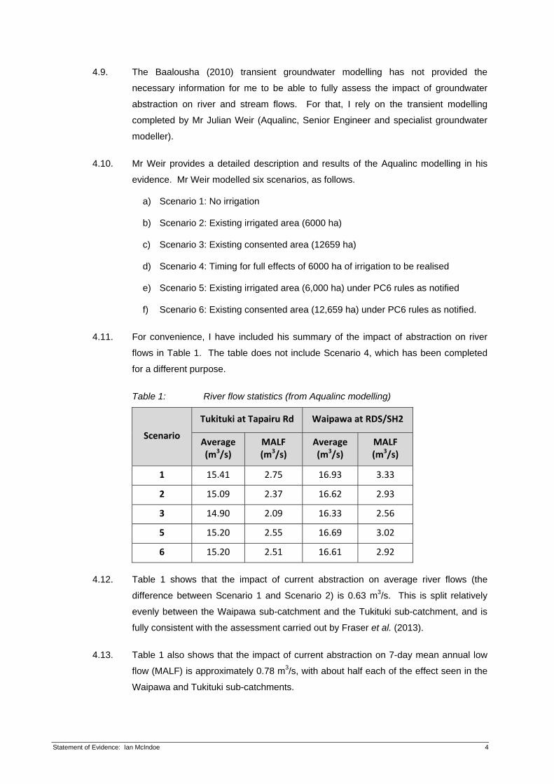
4.9. The Baalousha (2010) transient groundwater modelling has not provided the

necessary information for me to be able to fully assess the impact of groundwater

abstraction on river and stream flows. For that, I rely on the transient modelling

completed by Mr Julian Weir (Aqualinc, Senior Engineer and specialist groundwater

modeller).

4.10. Mr Weir provides a detailed description and results of the Aqualinc modelling in his

evidence. Mr Weir modelled six scenarios, as follows.

a) Scenario 1: No irrigation

b) Scenario 2: Existing irrigated area (6000 ha)

c) Scenario 3: Existing consented area (12659 ha)

d) Scenario 4: Timing for full effects of 6000 ha of irrigation to be realised

e) Scenario 5: Existing irrigated area (6,000 ha) under PC6 rules as notified

f) Scenario 6: Existing consented area (12,659 ha) under PC6 rules as notified.

4.11. For convenience, I have included his summary of the impact of abstraction on river

flows in Table 1. The table does not include Scenario 4, which has been completed

for a different purpose.

Table 1: River flow statistics (from Aqualinc modelling)

Scenario

Tukituki at Tapairu Rd Waipawa at RDS/SH2

Average (m3/s)

MALF (m3/s)

Average (m3/s)

MALF (m3/s)

1 15.41 2.75 16.93 3.33

2 15.09 2.37 16.62 2.93

3 14.90 2.09 16.33 2.56

5 15.20 2.55 16.69 3.02

6 15.20 2.51 16.61 2.92

4.12. Table 1 shows that the impact of current abstraction on average river flows (the

difference between Scenario 1 and Scenario 2) is 0.63 m3/s. This is split relatively

evenly between the Waipawa sub-catchment and the Tukituki sub-catchment, and is

fully consistent with the assessment carried out by Fraser et al. (2013).

4.13. Table 1 also shows that the impact of current abstraction on 7-day mean annual low

flow (MALF) is approximately 0.78 m3/s, with about half each of the effect seen in the

Waipawa and Tukituki sub-catchments.


4.14. The second question is whether the Plan Change 6 policies (as notified) have a

significant benefit on river flow regimes. Once again, I rely on the transient modelling

of Mr Weir to answer the question.

4.15. The benefit of PC6 compared to the current situation (the difference between

Scenario 5 and Scenario 2) is less than a 0.2 m3/s increase in average flows and less

than 0.3 m3/s increase in 7-day MALF. The benefit to the Tukituki River is greater

than to the Waipawa River.

4.16. The third and final question is what effect an increase in irrigated area relative to the

current area will have on the groundwater system and on river flows. For this

assessment, Mr Weir has assumed irrigated area will increase from the current 6,000

ha to 12,659 ha, which is allowed under current consents.

4.17. The current abstraction (pumping) would be expected to increase from about 23

million m3/year (consistent with Baalousha, 2010) to about 45 million m3/year. Some

of that pumped water will return to the groundwater system. Mr Weir has included the

impact of return water in his modelling.

4.18. I have no concerns about the groundwater system being able to sustain the increased

take. The full 45 million m3/year take is approximately 20% of the groundwater

average annual recharge. This is less than the NES recommendation. Once again,

localised interference effects would have to be managed.

4.19. Table 1 shows that under the existing rules, increasing the irrigated area will reduce

average flows in the Tukituki River by 0.19 m3/s and the Waipawa River by 0.29 m3/s

(Scenario 3 versus Scenario 2), making a total of 0.48 m3/s. It will reduce MALF in

the Tukituki River by 0.28 m3/s and in the Waipawa River by 0.37 m3/s, making a total

of 0.65 m3/s. The percentage decrease in MALF is lower than the percentage

increase in irrigated area.

4.20. Similarly, Table 1 shows that under PC6 rules, doubling the irrigated area will have

virtually no impact on average flows in the Tukituki River and the Waipawa River

(Scenario 6 versus Scenario 5). It will decrease MALF in the Tukituki River by 0.04

m3/s and in the Waipawa River by 0.10 m3/s. These are very small changes in my

view due primarily to allocation rules (restrictions).

4.21. Since the Aqualinc modelling was completed, HBRC has revised some aspects of the

Plan Change. In my view, the changes will have no material impact on my

conclusions. Removing the allocation limits on surface water resources will have no

impact. Modifying the stream depletion policies (TT11) could result in a decrease in

security of supply to some irrigators.


5. Background

HBRC’s Approach

5.1. The Hawke’s Bay Regional Council’s Regional Resource Management Plan (RRMP)

contains policies for managing surface water resources in the Tukituki Catchment,

including setting minimum flows and allocation limits. As I understand it, no

groundwater allocation limits or seasonal limits on water takes are included in the

RRMP. Plan Change 6 has taken a more integrated approach to manage surface

water and groundwater and proposes to fill the gaps in the RRMP.

5.2. In short, HBRC’s position is that current groundwater abstraction is having an adverse

effect on Tukituki Catchment river flows and therefore is impacting on in-stream

habitat requirements. They propose raising minimum flows and implementing

allocation limits, which they believe are needed to sustain river ecosystems and in-

stream values, while recognising that these measures will impact on security of supply

to existing users.

5.3. Although HBRC has attempted to quantify the effect of the proposed measures on

existing groundwater and surface water users (e.g. Waldron and Baalousha, 2013),

the robustness of the science behind the assessments has been questioned by the

RWUG. This has introduced a significant degree of uncertainty to RWUG members

on how they will be affected by the proposals.

Issues

5.4. The HBRC approach raises three fundamental issues for RWUG, which I address in

my evidence:


b) Does the proposed Plan Change 6 flow regime actually benefit the rivers in

terms of improved low flows?


5.5. I address each of these questions below.


Sustainability

5.6. The question of sustainability of existing takes relates to the impact of those takes on

groundwater levels and on surface water flows. I want to emphasise that a reduction

in aquifer storage, which is highlighted by Baalousha in evidence and in Baalousha

(2010), is not in itself an adverse effect. A reduction in aquifer storage is of little

consequence. Changes in aquifer storage result from changes in groundwater levels.

Whether changes in groundwater levels are adverse or not depends on what impact

they have on existing abstractive users, on surface water flows and on in-streams

users of the resource.

5.7. In the Ruataniwha Basin, because of the nature of the hydrogeology, groundwater

and surface water is clearly linked. If the current groundwater takes have significantly

lowered groundwater levels, or there is evidence of a continuing downward decline in

water levels, there is likely to be adverse effects on existing users of groundwater.

5.8. It follows that if there is a significant decline in groundwater levels, it is possible that

surface water flows will be significantly reduced in some locations at some time.

5.9. Hydrologically, groundwater abstraction has to be examined at two levels. The first is

at the catchment level – overall how much water is being removed from the catchment

relative to catchment inflow and what impact is that having on discharges from the

catchment.

5.10. The second is at a sub-catchment scale. The question is, what is the difference

between takes in different locations and at different depths on groundwater levels and

surface water flows.

5.11. I note that some of the current groundwater consents have minimum flow conditions

attached, mainly based on the generalised ‘400 metre’ policy (Policy 43) in the RRMP.

However, most of the existing groundwater takes are subject to daily flow limits or

weekly volume limits only. The different conditions on take consents will result in

different impacts on groundwater and surface water, which needs to be established.

Effects of Proposed Changes in Flow Regimes

5.12. If the current groundwater takes have significantly lowered groundwater levels or

there is evidence of a continuing downward decline in water levels, it is possible that

implementation of aquifer allocation limits may have value. If not, the implementation

of individual take limits on consents is unlikely to have a significant impact on the

groundwater system. It also means that it may be possible to allocate additional

groundwater.


5.13. Because HBRC proposes to fix the groundwater aquifer allocation limits at their

estimate of current volume taken, the groundwater allocation limits are unlikely to

change existing effects. However, the Plan Change 6 proposals include the raising of

minimum surface water flow limits, and it needs to be established whether or not that

will make any significant difference to surface water flows and/or to the groundwater

system.

5.14. Plan Change 6 also proposes to implement a more complex stream depletion

assessment of groundwater takes, similar to that currently used by Canterbury

Regional Council. Whether that will increase or decrease the number of groundwater

takes subject to minimum flow conditions and to what degree, has not been

established by HBRC. It follows that further investigation is required to establish the

benefits or otherwise of implementing the revised policies.

Increasing Groundwater Takes

5.15. Most of the analysis completed by HBRC on the effects of groundwater abstraction on

river flows has been on the basis of current irrigated area being about 6000 ha,

abstracting in the order of 23 million m3 of water annually. Policies and limits have

largely been built around those estimates. In the HBRC expert evidence, I notice that

the estimate has been increased to 7,000 ha and 25 million m3.

5.16. The potential irrigated area under current consents is significantly larger, and may be

up to 13,000 ha. Because existing water permits generally don’t include seasonal

volume limits, it is realistically possible for irrigated area and the volume of water used

to increase. This scenario has not been considered by HBRC, because of the view

that the groundwater system is fully or even over-allocated.

Scope of Evidence

5.17. My evidence is aimed at providing answers to the issues raised above. My evidence

addresses the impacts of the relevant proposed Plan Change 6 policies on existing

groundwater takes and on river flows in the Ruataniwha Basin. I have not directly

considered the impact of the Plan Change 6 policies beyond the Ruataniwha Basin;

neither have I specifically considered the impact of the proposed Makaroro water

storage dam and irrigation scheme on river flow regimes or on groundwater.

5.18. In preparing my evidence, I have:

a) Reviewed investigations completed for RWUG into the likely impacts of Plan

Change 6 policies.

b) Summarised the relevant Plan Change 6 policies in the context of Ruataniwha

Basin groundwater and surface water.


c) Reviewed relevant current information relating to Plan Change 6 and its effects

on Ruataniwha groundwater and surface water.

d) Described the structure of the groundwater system based on hydrogeological

information to better understand cause and effect relationships related to

surface water and groundwater.

e) Summarised the key inputs and outputs to and from the hydrological system.

f) Assessed the effect of the current abstractions on the overall water balance.

g) Described the relationship between groundwater levels and flows in

streams/rivers.

h) Assessed the effect of existing groundwater abstraction on groundwater levels,

rivers, and stream flows at a sub-catchment level under current permit

conditions.

i) Assessed the effect of current groundwater abstraction on groundwater levels,

rivers, and stream flows at a sub-catchment level under proposed Plan Change

6 policies.

j) Assessed the effect of increased groundwater abstraction from the Ruataniwha

aquifers.

Irrigation Security of Supply

5.19. Evidence on the impact of the Plan Change 6 proposals related to seasonal volumes

and minimum flows and how they impact on the hydrological aspects of irrigation

security of supply is presented by Dr John Bright.

Sources of Information

5.20. My sources of information are:

a) Proposed Plan Change 6 – Tukituki Catchment, notified 4 May 2013.

b) S32 Evaluation Summary Report (Plan Change 6 – Tukituki Catchment).

c) Report No C12064/3, Aqualinc Research Ltd, June 2013.

d) Ruataniwha Plains Water Resources - Review of groundwater management

investigations (Ballard, 2012)

e) The HBRC reports referenced in my evidence.

f) The HBRC evidence of R Van Voorthuysen, H Baalousha, P Barrett, M

Thorley, D Leong and R Waldron.


6. Evidence Proper

Previous Aqualinc Investigations

6.1. My evidence builds on previous Aqualinc investigations carried out for the Ruataniwha

Water Users Group to look at groundwater management issues in the Ruataniwha

Basin, the results of which have been presented in two reports. The first (Ballard,

2012) reviewed the key project reports describing the investigations undertaken by

Hawke’s Bay Regional Council to underpin changes in the management of

Ruataniwha Plains water resources.

6.2. The second (Fraser et al., 2013) provided a comprehensive assessment of the effects

on the mean annual outflow of water removed from the Ruataniwha Basin due to

irrigation, based on a water balance analysis. The report also included a preliminary

modelling assessment of the effects of groundwater takes on low flows in the

Waipawa and Tukituki Rivers.

6.3. Throughout the HBRC reports, one of the justifications provided by HBRC for

conducting the investigations was the assertion that groundwater pumping has

adverse impacts on groundwater resources and that this is leading to reductions in

spring-flows and causing the groundwater-fed river sections to run dry.

6.4. Ballard (2012) found that this assertion was not supported by robust evidence to

demonstrate any change in river flow or groundwater levels and that evidence by way

of measured data and model results would be needed to provide support for this

assertion. Such evidence had not been presented at the time the Ballard review was

completed.

6.5. The main issue raised by Ballard (2012) was that there were significant shortcomings

in the groundwater modelling used by HBRC to support their position. The steady

state groundwater modelling is reported in Baalousha (2009a), while the transient

modelling is reported in Baalousha, (2010). The problems identified by Ballard (2012)

were:

a) The number of significant, inappropriate, approximations and inconsistencies

that exist in the data used in the groundwater modelling studies.

b) Weaknesses in the model development and testing process (it does not follow

good practice).

c) Inadequacies in how the groundwater model has been used to assess the

impact of current pumping, potential pumping and potential water harvesting.


6.6. Since those reviews have been completed, HBRC have proposed restricting existing

and future groundwater takes through Plan Change 6. However, the key question “Is

the current situation sustainable” still remained unanswered. Although HBRC has

used the transient model to assess the effects of the proposed plan changes on river

flows and security of supply for existing consent holders, (e.g. Waldron et al., 2012),

as far as I am aware, the model still contains many of the problems identified by

Ballard (2012).

6.7. One of the objectives of the Fraser et al. (2013) investigation was to gain a better

understanding of the impact of current Ruataniwha Basin groundwater abstraction on

the groundwater aquifer underlying the Plains and on the Tukituki River and Waipawa

River flows.

6.8. The study found that, based on an irrigated area of 13,000 ha (which is the area

assigned to current consents, not the area actually irrigated):

a) Even without abstractions for irrigation, groundwater levels in monitoring bores

would have decreased during the period 1992 to 2003.

b) Long-term mean annual river flows are expected to be lower under the

irrigation scenario relative to the zero irrigation scenario by 4.5% and 3.2% for

the Tukituki and Waipawa Rivers, respectively, but vary from year to year.

c) The impacts of taking and using water for irrigation are greater in the Tukituki

sub-catchment than in the Waipawa sub-catchment.

d) Indicatively, low-flows in the Tukituki River would be reduced by approximately

0.6 m3/s, or 8% of the modelled “No irrigation” low-flow. Low-flows in the

Waipawa River would be reduced by approximately 0.35 m3/s, or 7% of the

modelled “No irrigation” low-flow.

6.9. The preliminary flow reductions determined by Fraser et al. (2013) are less than that

reported by HBRC, these being 23% and 10% for the Tukituki and Waipawa Rivers

respectively, despite the HBRC assessment being based on only 6,000 ha of

irrigation.

Aqualinc Groundwater Modelling

6.10. To support the Fraser et al. (2013) investigation, a groundwater-surface model of the

Tukituki Catchment/ Ruataniwha Basin was developed by Aqualinc and was used to

assess the approximate effects of groundwater abstractions on river flows. Although it

was a first-cut approach to modelling these relationships, my understanding is that it

was constructed in a way that eliminated the HBRC model problems.


6.11. The model has recently been updated, recalibrated and used by Mr Weir to test a

number of scenarios relating to the Plan Change 6 proposals. Mr Weir is presenting

expert evidence on the model development and use.

6.12. Mr Weir has used the model to predict the response of the groundwater system to

changes in groundwater allocation, groundwater development (abstraction), and

changes to Tukituki Catchment river minimum flows and flow regimes resulting from

the Plan Change 6 proposals. I have used information from the model to corroborate

and support the evidence I have presented.

Proposed Plan Change 6 – Tukituki Catchment

6.13. The most significant plan changes likely to impact on consented water takes (surface

water and groundwater) in the Ruataniwha Basin are:

a) The proposed change to minimum flow limits on various streams and rivers in

the catchment. These are proposed to be managed from seven flow

management sites. A description of the proposed minimum flows and timetable

for implementation is given in Table 5.9.3 in the Proposed Plan.

b) The implementation of the minimum flow limits on surface water takes and

groundwater takes with a high1 stream depletion classification as described in

POL TT11 in the Plan.

c) Setting surface water and groundwater allocation limits that are based on the

existing volume of consented abstraction (Tables 5.9.4 and 5.9.5 in the Plan).

d) Allocating surface water at high flows (flows above the median), as described in

Table 5.9.6.

e) Implementing seasonal volumes on existing consented takes, which is the

lesser of (i) the volume assessed in accordance with Policies 32 and 42 or (ii)

using the procedure set out in Schedule XVII (for irrigation takes, paragraphs 6

and 7).

6.14. HBRC also proposes to not reallocate water that is “freed up” through surrender of

existing consents or through the implementation of POL TT9(1)(a) - annual volume

limits.

6.15. Plan Change 6 proposes raising the minimum flows of rivers to increase the flows

available for environmental needs. This is to be done in steps over a defined

timeframe. My understanding of existing and proposed final minimum flows relevant

to the RWUG is given in Table 2.

1 HBRC are now proposing in their evidence a new ‘direct’ stream depletion category This will not materially affect my conclusions.


Table 2: Existing and proposed minimum flows

Site Current

minimum flow (l/s)

Proposed minimum flow (l/s)

Tukipo River (SH50) 150 n/a

Tukipo River (Ashcott Rd) n/a 1,043

Tukituki River (Tapairu Rd) 1,900 2,300

Waipawa River (RDS/SH2) 2,300 2,500

Tukituki River (Red Bridge) 3,500 5,200

Papanui Stream (Middle Rd) 53 53

Mangaonuku Stream (U/S Waipawa) n/a 1,170

6.16. The proposed implementation of the minimum flow steps over time are given in Table

5.9.3 under POL TT8.

6.17. Surface water allocation limits are given in Table 5.9.4 also under POL TT8. Three

major surface water zones and three surface water sub-catchment zones have been

proposed, with flow (litres/sec) and volumetric (thousand m3/year) limits given. I note

that in evidence, HBRC are now proposing to remove the volumetric limits.

6.18. Table 20 in the S32 Evaluation Summary shows that the surface water allocation

limits proposed under Plan Change 6 are essentially the same as what has been

assigned to current consents. Flow information will have generally been stated on

consents, while the annual volumes will have been assessed by HBRC.

6.19. Groundwater allocation limits are given in Table 5.9.5 also under POL TT8. HBRC

has divided the groundwater resources in the Tukituki Catchment into three allocation

zones for managing the volume of groundwater allocated from each groundwater

resource.

6.20. The Ruataniwha Plains has been divided into two allocation zones for managing the

effects of groundwater abstraction on surface water. These two zones are termed

Ruataniwha Basin - Groundwater Management Zone 2 and Zone 3. They generally

align with the surface water catchments of the Waipawa and Tukituki rivers (Codlin,

2012). The third groundwater allocation zone is the Otane Basin - Groundwater

Management Zone 1 located in the Papanui Catchment area, which contains a

separate groundwater resource.


6.21. HBRC has set the groundwater allocation limits (m3/year) for the three zones at the

currently assessed groundwater consented volumes. The HBRC’s groundwater team

estimated that the current level of groundwater abstraction equated to 31% of current

groundwater allocation.

7. General Description of the Environment

Key Hydrological Features

7.1. The Tukituki Catchment has been described in detail in many documents. I have

summarised what I see as the most relevant key hydrological features below.

7.2. The Tukituki catchment is one of the larger catchments in Hawke’s Bay covering

approximately 2500 km². The Tukituki River flows north from southern central

Hawke’s Bay into the Pacific Ocean near Haumoana, south of Napier. The mean

annual flow is 43.848 m3/s at Red Bridge in the lower end of the catchment.

7.3. The largest tributary of the Tukituki River is the Waipawa River, draining the Ruahine

Ranges north of the Tukituki. Also in the north the Mangaonuku River flows into the

Tukituki River draining the Wakarara Ranges. Joining the Tukituki River from the

south are the Tukipo, Makaretu, Porangahau and Mangatarata rivers, while the

Maharakeke River drains the Turiri Range. These tributaries join the Tukituki River

after flowing across the Ruataniwha Plains, in the central part of the catchment.2

7.4. The Tutituki-Waipawa River confluence is about 5 km east of the township of

Waipawa. About 6 km north-east of the confluence of the Tukituki and Waipawa

Rivers, the Tukituki River flows in a northerly direction through a narrow valley or

more constrained area known as the upper corridor, eventually reaching the southern

end of the Heretaunga Plains near Havelock North. From there it flows across the

plains to the Pacific Ocean.

7.5. The Ruataniwha Basin lies within the Upper Tukituki River catchment, in the south of

Hawke’s Bay Region, New Zealand (see Figure 1).

2 From: http://landandwater.co.nz/councils-involved/hawke-s-bay-regional-council/tukituki-river


Figure 1: Location map of the Ruataniwha plains (from Fraser et al., 2013)

7.6. The catchment upstream of the confluence of the Tukituki River and the Waipawa

River has a total area of 1,472 km2 (Baalousha, 2009). The Ruataniwha basin is

approximately 800 km2 of this area (Baalousha, 2009). The catchment ranges from

approximately 150 metres above sea level (m amsl) at the outlet in the east to

approximately 1,700 m amsl in the west (Ludecke, 1988).

7.7. The most productive of the groundwater resources in the Upper Tukituki catchment is

located beneath the Ruataniwha Plains. The Otane Basin, located in the Papanui

Catchment area, also contains groundwater resources.

7.8. At the lower end of the catchment, the Tukituki River intersects with the Heretaunga

Plains and forms the lower Tukituki aquifer system. This lower Tukituki aquifer

system overlies and merges with the main aquifer system of the Heretaunga Plains.

The effects of groundwater development in the lower Tukituki aquifer are considered

best managed as part of the Heretaunga Catchment (Harper, 2013).

7.9. The Ruataniwha Water Storage project proposes building a 90 million m3 dam in the

upper Makaroro River in the Wakarara Ranges. The Makaroro River joins the

Waipawa River near Springhill, which means that the dam releases will impact on the

Makaroro River flows, the Waipawa River flows and ultimately, the lower Tukutuki

River flows.

Tukituki Catchment River Flows

7.10. Naturalised flows for the Tukituki River major sub-catchments have been estimated by

HBRC. Mean annual flow (MAF), median flow and mean annual low flow (MALF) are

given in Table 3 below.


Table 3: Naturalised flows (cumecs) for major sub-catchments of the Tukituki River (Wilding & Waldron, 2012).

Code Site Mean Median MALF

T1 Waipawa River at RDS/SH2 14.97 8.99 3.01

T15 Tukituki River at Tapairu Rd 15.83 9.83 2.86

T16 Tukituki River at Red Bridge 44.51 22.02 6.26

T17 Makaroro River at Burnt Bridge 6.66 3.68 1.39

7.11. To determine the “naturalised” flow record for the Tukituki River at the exit to the

Ruataniwha basin, HBRC firstly developed “naturalised” flow estimates for the

Waipawa River at RDS/SH2 and Tukituki River at Tapairu Road by synthesising daily

flow records from measured data and adding the estimated surface water and

hydraulically connected groundwater abstractions from the rivers onto the actual

observations of flow to provide an estimate of the natural flow. These naturalised flow

records for Waipawa at RDS/SH2 and Tukituki River at Tapairu Road were then

summed together to estimate the Basin outflows. (Waldron, et al., 2013, Appendix 3).

7.12. Given the significant degree of synthesis required to generate flow records, the

naturalised flow records must be used with caution.

7.13. I note that the mean naturalised flow for the Tukituki River at Red Bridge is 44.5 m3/s,

compared to an actual mean flow of 43.8 m3/s. This is a reduction of 0.7 m3/s.

8. Hydrogeology: The Aquifers and their Characteristics

Description of Aquifers

8.1. To be able to assess the impact of current groundwater abstraction on groundwater

levels, storage and stream flows, an understanding of the nature of the groundwater

connection with rivers and streams is necessary.

8.2. The Ruataniwha Basin contains two main water-bearing formations. The shallow

gravels are known as the Young formation, which overlay older gravels known as the

Salisbury formation. According to Harper, (2013), the Salisbury gravels are the most

productive, while the Young gravels are more permeable and less consolidated,

although he states that the Young formation contains the majority of wells within the

basin.


8.3. There are also other water-bearing formations such as the limestone deposits south of

Lake Poukawa and less productive aquifers in the Papanui area and on the fringes of

the Ruataniwha Plains.

8.4. The geology of the aquifers is adequately described in several reports including

Gordon (2013), Harper (2013) and (Baalousha, 2009). The hydrogeology is also

described. A key point is that each formation contains a number of water bearing

layers resulting in a wide variation in bore depths.

8.5. Francis (2001) makes the point that the distinction between the Young gravels and the

Salisbury gravels is unclear. Harper (2013) states that the Young formation is

unconfined, while the Salisbury formation is confined. I have seen no evidence to

support the statement that the Younger formation is unconfined and that the Salisbury

formation is confined. Given the high degree of variability in bore depths and water

bearing layers, and the lack of evidence of confining layers in bore logs, it is more

likely that the Young formation is leaky unconfined and the Salisbury formation leaky

confined (semi-confined) as described by PDP (1999). I agree with Baalousha (2009)

that the basin is very heterogeneous and that the aquifers are connected, although

the degree of connection from one water bearing layer to another will differ.

Aquifer properties (T, S, L and Other Properties)

8.6. Key aquifer properties are transmissivity (for all aquifers), storativity (for confined or

semi-confined aquifers), specific yield (for unconfined aquifers) and leakage (for leaky

aquifers). With respect to groundwater–surface water interactions, streambed

conductance is also important. While transmissivity can be obtained from simple

aquifer step-tests, the other parameters need to be derived from properly conducted

aquifer tests using appropriately located observation bores.

8.7. Transmissivity is a measure of how easily water is able to move through an aquifer.

Horizontal transmissivity values from aquifer tests are given in Baalousha (2010)

Figure 7, and range from 30-10,000 m2/d. I don’t know how reliable these values are.

A value of 30 m2/d would indicate a very low producing aquifer, while 10,000 m2/d

would indicate a very high producing aquifer. Clearly, there is a high degree of

variability in the values, and the only general conclusion that can be made is that the

higher transmissivity areas appear to be closer to the Waipawa River.


8.8. Storativity provides a measure of how much water can be released from aquifers due

to a change in pressure or water level. I have been unable to source storativity values

from aquifer test data, and am relying on the values from Baalousha (2010) which

were not measured, but obtained from groundwater modelling. The published values

range from 0.1-0.3 for unconfined aquifers and 0.00006-0.006 for confined aquifers,

although I note that the confined aquifer values are specific storage, not storativity.

8.9. The values are within normal ranges for leaky unconfined and leaky confined aquifers,

but again, I do not know how reliable they are. I disagree with Harper (2013) that high

specific storage means the aquifer beneath the Waipawa River is able to release

groundwater more easily. High specific storage means that more groundwater can be

released per unit change in pressure or head, but transmissivity and streambed

conductance will determine how easily that water is released.

8.10. I have no information on measured leakage values. Baalousha (2010) has assumed

a ratio of vertical to horizontal hydraulic conductivity of 0.1 for his modelling. I cannot

comment on how good that assumption is, except to say that vertical hydraulic

conductivity is always lower than horizontal hydraulic conductivity in alluvial aquifers.

8.11. I also have no information on streambed conductance for the rivers in the Ruataniwha

Basin. Baalousha (2010) states that riverbed conductance is one of the most

uncertain variables and that no field data is available. The estimated values used by

Baalousha ranged from 5 m2/d for small streams up to 6,000 m2/d for large rivers. I

am unable to comment on the relevance of these values.

Summary of the Groundwater System

8.12. My summary of the groundwater system in the Ruataniwha Basin is:

a) There are two formations (Young and Salisbury), but because of the lack of

evidence of consistent aquitards, there is no clear definition of aquifers.

“Aquifers’ are more likely to be preferred water bearing zones.

b) There is very little verifiable field data on basic aquifer parameters, particularly

leakage coefficients and stream-bed conductance.

c) The available measured data indicates that there is a high degree of spatial

variability.

d) The shallow water bearing layers are likely to be less confined than the deeper

layers. This implies that shallow groundwater will be connected to streams and

rivers and that the connection between shallow groundwater and deep

groundwater will be slow.


Surface Water-Groundwater Interactions

8.13. Where river water levels are higher than groundwater levels at a particular location

and where the bed of the river is permeable, a river is able to recharge groundwater.

Conversely, where river water levels are lower than groundwater levels, groundwater

is able to recharge a river.

8.14. There are three primary ways of identifying interchanges of river water and

groundwater. They are:

a) Flow gauging of river flows to determine gaining and losing reaches. Visual

observations of rivers drying up or regaining flows may also be apparent.

Some gauging has been carried out (Johnston, 2011).

b) Groundwater-surface water modelling (numerical and empirical). Numerical

modelling has been carried out (Baalousha, 2010), but river flow gauging data

has not been used to calibrate the model.

c) Water chemistry. There is limited data on this (Undereiner et al., 2009).

8.15. Despite the limited measured data, several HBRC reports refer to groundwater-river

water interactions in the Ruataniwha Basin and in the Heretaunga Plains. These

include Brooks (2006), Harper (2013), Wilding & Waldron (2012), and (Baalousha,

2010). These reports reference many other studies carried out to describe and

attempt to quantify these interactions.

8.16. What appears to be generally agreed is that groundwater and surface water

interactions occur to some degree along most of the Tukituki and Waipawa river

reaches across the Ruataniwha Plains (Baalousha, 2009, Morgernstern et al, 2012).

It also appears that some interaction occurs in the minor tributaries towards the

bottom of the basin.

8.17. Figure 10 in Baalousha (2010) shows a rough approximation of gain-loss patterns of

rivers and streams in Ruataniwha, referenced to Hawke's Bay Regional Council,

(2003). He concludes that the main rivers (Waipawa and Tukituki) are losing in the

west of the basin and drying in the east, as they leave the basin. The longest dry

reach occurs on the Waipawa River before the Mangaonuku River joins it, as the

gravel in the area is thick and highly permeable. It is believed that most of river water

is lost to adjacent springs and the Kahahakuri Stream (Hawke's Bay Catchment Board

& Regional Water Board, 1984).


8.18. Tonkin & Taylor (2012) noted that the Young gravels are a product of historic and on-

going deposition by the river and as a result of this deposition, the river channel can

become perched higher than the surrounding land and hence higher than the

groundwater level.

8.19. According to Wilding & Waldron (2012), Johnson (2011) investigated the loss and

gain of stream flow to groundwater, based on concurrent gaugings across the

Ruataniwha Plains during 2009.

8.20. A key output from Johnson’s report was a map showing the spatial distribution of

streams that lose or gain flow (Figure 10 in Wilding and Waldron (2012) taken from

Johnson (2011)). In particular, Johnston indicated that the Waipawa, Tukituki and

Makaretu rivers lost flow over considerable lengths of stream, particularly as they

traversed more recent alluvial deposits of the eastern Ruataniwha Plains (from HBRC

2003).

8.21. Apparently, the lost flow was regained at the eastern edge of the Ruataniwha Plains

as well as from spring-fed tributaries. For that to happen, the spring-fed tributary bed

levels must be below groundwater levels, because of a relatively deeper channel or

because the channel was at a lower elevation. Whether all of the flow or just some of

the flow was regained, I do not know.

8.22. Using chemical signatures, Undereiner et al. (2009) concluded that springs closer to

the Waipawa River have a more direct connection to river water via the shallow

aquifer. The lower elevation Mangaonuku Stream intercepts springs on the eastern

edge of the plains that drain both the shallow aquifer and the deep aquifer.

8.23. According to Johnson (2011), the Tukituki River downstream of the Waipawa

confluence demonstrated little gain or loss of flow during 2009 gaugings. Johnson

attributed the lack of loss/gain in the lower river to the small alluvial aquifer, which is

bounded by basement rock within a narrower valley.


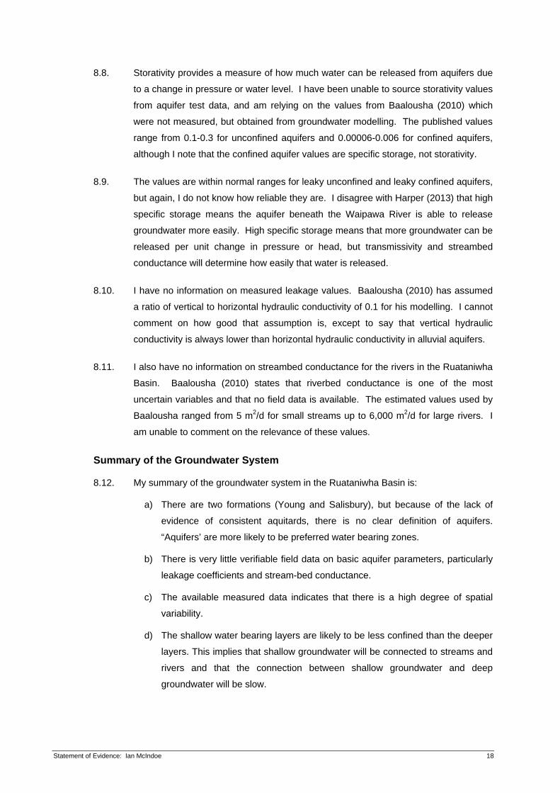
Figure 2: Indicative location of "losing" and "gaining" river reaches in the upper and middle Tukituki catchment (From Johnson 2011).

Conclusions Regarding Surface Water-Groundwater Interaction

8.24. I can conclude from the available data that the streams and rivers within the

Ruataniwha Basin interact with groundwater. In some locations surface water leaks to

groundwater. In other areas, particularly towards the bottom of the Basin,

groundwater is discharging to surface water.

8.25. My view is that the majority of groundwater discharging to surface water is shallow

groundwater, which is consistent with the aquifer description. The exception may be

in the lower Mangaonuku River where chemical signatures have indicated some

discharge of deeper groundwater, but I have no detailed information to confirm that.


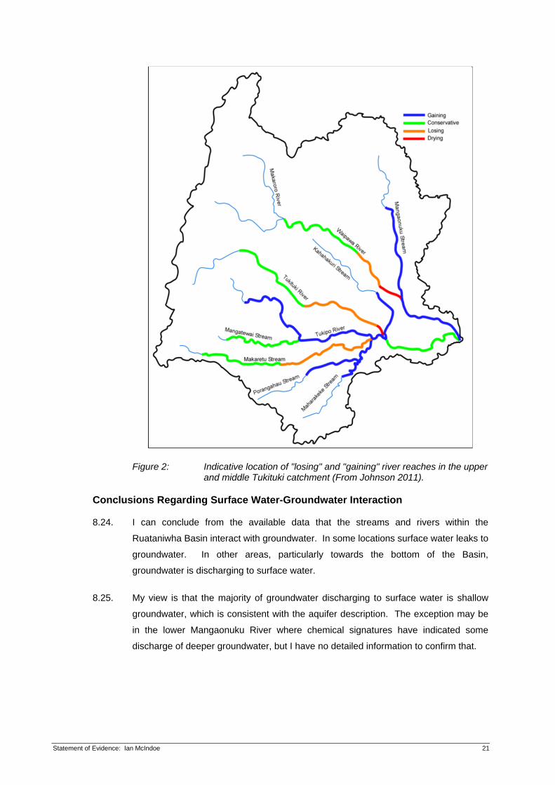
8.26. The two largest rivers, the Tukituki and Waipawa, appear to lose a significant amount

of flow to groundwater, while the nearby Mangaonuku and Tukipo Rivers gain flow

from groundwater. This may simply be due to the relative height of riverbed relative to

groundwater level implying that the larger rivers have become perched above the

groundwater table, while the others have cut into the gravels below the water table.

9. The Hydrological System

The Overall Water Balance

9.1. One of the most important hydrological features of the Ruataniwha Basin and the

upper catchment is that water entering the catchment as rainfall leaves the catchment

as evaporation, transpiration, or river flows through the upper corridor. There are no

other water transfers into or out of the catchment except perhaps a small groundwater

flow through the upper corridor, which may not be picked up in Tukituki river flow

measurements.

9.2. In terms of the catchment overall, this feature makes it more straight-forward to

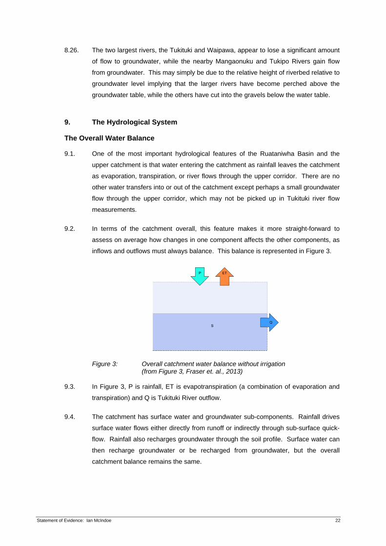
assess on average how changes in one component affects the other components, as

inflows and outflows must always balance. This balance is represented in Figure 3.

Figure 3: Overall catchment water balance without irrigation (from Figure 3, Fraser et. al., 2013)

9.3. In Figure 3, P is rainfall, ET is evapotranspiration (a combination of evaporation and

transpiration) and Q is Tukituki River outflow.

9.4. The catchment has surface water and groundwater sub-components. Rainfall drives

surface water flows either directly from runoff or indirectly through sub-surface quick-

flow. Rainfall also recharges groundwater through the soil profile. Surface water can

then recharge groundwater or be recharged from groundwater, but the overall

catchment balance remains the same.


9.5. Evaporation can be directly from surface water features (rivers, streams, lakes), from

the ground surface, or transpired through plants. Evapotranspiration (ET is a

combination of evaporation and transpiration) takes water out of the catchment,

lowering river flows and groundwater levels.

9.6. Evapotranspiration under non-irrigated conditions is limited by how much rainfall is

stored in the soil that can be used by plants. During wet periods, actual ET (AET)

may approach a potential level (PET), but during droughts AET can be reduced to

close to zero.

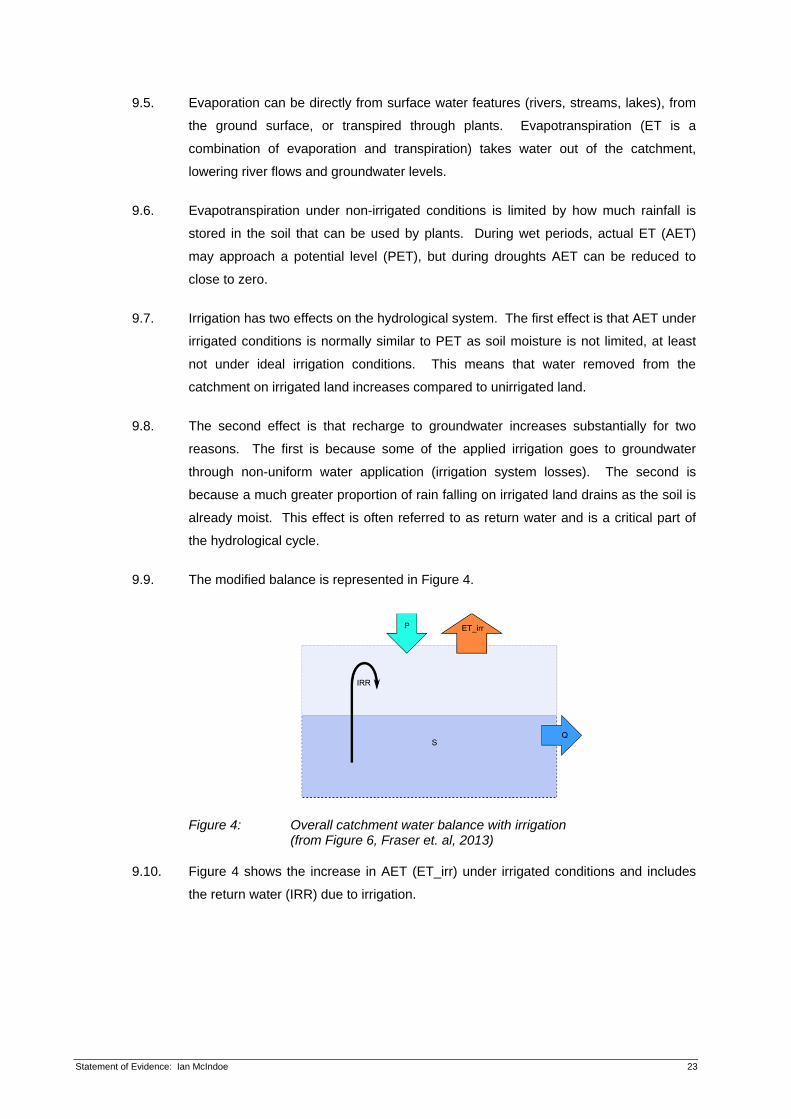
9.7. Irrigation has two effects on the hydrological system. The first effect is that AET under

irrigated conditions is normally similar to PET as soil moisture is not limited, at least

not under ideal irrigation conditions. This means that water removed from the

catchment on irrigated land increases compared to unirrigated land.

9.8. The second effect is that recharge to groundwater increases substantially for two

reasons. The first is because some of the applied irrigation goes to groundwater

through non-uniform water application (irrigation system losses). The second is

because a much greater proportion of rain falling on irrigated land drains as the soil is

already moist. This effect is often referred to as return water and is a critical part of

the hydrological cycle.

9.9. The modified balance is represented in Figure 4.

Figure 4: Overall catchment water balance with irrigation (from Figure 6, Fraser et. al, 2013)

9.10. Figure 4 shows the increase in AET (ET_irr) under irrigated conditions and includes

the return water (IRR) due to irrigation.


9.11. If we assume that the system is in balance and compare Figure 3 and Figure 4, the

only additional water leaving the hydrological system due to irrigation is the additional

ET on the irrigated area, which is (ET_irr – ET). If we know the irrigated area, we can

easily calculate the effect of irrigation on the catchment. If the system is in balance,

the additional ET out of the system must result in an equivalent reduction in Tukituki

outflow (Q), given the closed nature of the system.

9.12. This analysis has been completed by Fraser et. al., (2013). For an irrigated area of

13,066 ha, Fraser et. al., concluded that the reduction in mean river flow would be in

the order of 1.3 m3/s.

9.13. Assuming the change is proportional to irrigated area, if 6000 ha is actually irrigated

(from Baalousha, 2010), the mean effect on river flows at Red Bridge determined by

Fraser et. al. (2013) is likely to be in the order of 0.6 m3/s. If irrigated area was not

fully irrigated, the mean effect will be lower, but on no account can it be higher. I

noted in my paragraph 7.13 that measured river flows are 0.7 m3/s lower than

synthesised naturalised flows, which is consistent with the 0.6 m3/s determined above.

9.14. Average rainfall entering the catchment is 1,304 mm/year, which equates to 60.9

m3/s. Average water leaving the catchment (Red Bridge Tukituki flows) is 30.6 m3/s.

Irrigation (6,000 ha) is responsible for removing 0.6 m3/s, which is less than 1% of the

total catchment inflow and about 2% of mean river flow. The 29.7 m3/s remainder,

which is about half of the water entering the catchment, is removed by

evapotranspiration throughout the catchment.

9.15. The key conclusion that comes out of this analysis is that rainfall dominates the

overall balance. Irrigation abstraction (through increased ET) is currently a distinctly

minor factor in the balance.

Spatial and Temporal Effects of Irrigation

9.16. How the surface water and groundwater sub-components of the hydrological system

are affected overall by irrigation depends on whether the supply of water for irrigation

comes from surface water or groundwater.

9.17. If the supply is from surface water, surface water flows will logically decrease, and

shallow groundwater will be partly recharged with surface water (due to non-uniform

application of irrigation), and partly with additional rainfall recharge, which will raise

shallow groundwater levels.


9.18. The increase in shallow groundwater levels could decrease river water recharge to

shallow groundwater in areas where the water level gradient between surface water

and groundwater is small. It could increase leakage to deeper aquifers, but that effect

will be small, given the nature of the groundwater system. Most likely, the additional

recharge will discharge relatively quickly back to surface water via springs and

seepage, as explained in Paragraph 9.45. The overall net effect on surface water

flows is reduced compared to the effect of the take alone.

9.19. If the supply is from groundwater, groundwater levels or pressures will decrease due

to the abstraction. If the take is from shallow groundwater, the lowering of

groundwater levels will be partly compensated by return water from irrigation system

losses and additional rainfall recharge. The net effect of lower groundwater levels

could increase river water recharge to groundwater in some areas and decrease

groundwater flows to rivers and springs in other areas.

9.20. If the take is from deeper groundwater, the return water will increase shallow

groundwater levels, and in extreme cases may result in mounding of shallow

groundwater. The compensatory effect of the return water on groundwater levels or

pressures at the depth of the take reduces as the depth of take increases.

Correspondingly, the amount of quick recharge back to springs and streams increases

as the depth of take increases.

9.21. Irrigating from deep groundwater aquifers where the deep aquifers are leaky confined

(or confined) effectively transfers deep groundwater to shallow groundwater. With the

additional return water from rainfall, this can have a significant influence on shallow

groundwater and spring flows. This effect is well-known in other areas in NZ where

drainage systems are sometimes required to remove the shallow groundwater.

9.22. One of the key criticisms of the Baalousha (2010) groundwater model is that it does

not account for irrigation return water. This omission has been highlighted by Ballard

(2012) and Golder (Appendix D in Aquanet, 2013). It is my view and the view of my

colleagues that irrigation return water must be included in groundwater modelling if

one of the key purposes of the modelling is to quantify the effects on groundwater

abstraction on stream flows.

Groundwater System Dynamics

9.23. As in most catchments, the hydrological system in the Ruataniwha Basin is not in a

steady state because the inputs and outputs are constantly changing. Rainfall varies

day by day and year by year. River flows, groundwater and surface water

abstractions, groundwater storage and actual evapotranspiration are constantly

changing.


9.24. The hydrological system is responding to these changes by moving towards an

equilibrium state. However, it never truly reaches equilibrium because of the

continuing change in inputs and outputs. It is this dynamic nature of the system that

makes it more challenging to assess the effects of changing one component of the

water balance on other components.

9.25. If we wish to assess the effects of irrigation abstractions on river flows or on

groundwater levels, we could, for example, compare trends in irrigation abstractions

with river flow statistics, or with groundwater level trends. However, that may lead to

incorrect conclusions because the trends may be due to other factors, in particular

rainfall and rainfall recharge, given the dominance that rainfall has on the water

balance.

9.26. Figure 5 summarises the annual land surface recharge for the period 1973-2011 at an

example location approximately mid basin (this data was supplied to me by Dr Bright

and Mr Weir). This data is the net groundwater recharge that enters the regional

aquifer system after the quick recharge has moved to surface waterways (as

discussed in Mr Weir’s evidence).

Figure 5: Ruataniwha rainfall recharge

9.27. This record indicates a slight downward trend in rainfall recharge (~1 mm/year) over

the period presented. Six years of high recharge (1974, 1976, 1977, 1979, 1980 and

1992) have been experienced in the record.

0

50

100

150

200

250

1973

1974

1975

1976

1977

1978

1979

1980

1981

1982

1983

1984

1985

1986

1987

1988

1989

1990

1991

1992

1993

1994

1995

1996

1997

1998

1999

2000

2001

2002

2003

2004

2005

2006

2007

2008

2009

2010

2011

Land surface recharge (mm/year)

Year

Net Land Surface Recharge


9.28. Figure 13 of Harper (2013) presents a graph of groundwater level trends for the 2003-

2013 years for a single well (Bore 5006) in Drumpeel Road. Based on a seasonal

Kendal test, Mr Harper identified a downward trend in groundwater levels of 8

cm/year. Given the relatively short record and the fact that it is based on a single well,

it is difficult to draw hard conclusions about trends. All that can be stated is that for

this well in this location, there could be a downward trend.

9.29. According to Baalousha (2010), groundwater abstraction has increased six-fold since

2010. His data is given in Figure 6 below.

9.30. It is tempting to conclude from Figure 6 that irrigation abstractions, given the large

relative increase in volumes taken since 1997 in particular, are causing a downward

trend in groundwater levels. Logically, I would expect that irrigation abstractions are

having some effect in some locations at some time, but where and when has not been

established in my view.

Figure 6: Annual groundwater abstraction (from Baalousha, 2010)

9.31. Bore water level records can provide some insight into the nature of the groundwater

system, and how it works. I have examined the water level records of 29 bores in the

Ruataniwha Plains (locations are shown in Figure 7) to better understand groundwater

dynamics in the catchment.


Figure 7: Bore locations.

9.32. I am of the opinion that the water level records from the bores shown in Figure 7 are a

good representative sample of groundwater levels in the Ruataniwha Basin. The

bores are dispersed over the basin, range in depth from 3.3 m to 110 m and are at

various distances from rivers and streams.

Groundwater Abstraction at the Basin Scale

9.33. At the basin scale, the volume of water abstracted from the groundwater system

relative to the amount of groundwater flowing through the aquifers and relative to the

amount of land surface recharge can provide some insight into the likely impact of

abstraction on the groundwater system. We know from my statement in Paragraph

9.14 that the amount of water removed from the catchment due to irrigation is very

small relative to total catchment inflows and outflows. We need to establish the

significance of groundwater abstraction on the groundwater system.

9.34. It has been established that groundwater flows in a direction from the western edge of

the Ruataniwha Basin down towards Waipukurau (see Baalousha, 2010, Figure 11,

Figure 28). The groundwater levels drop about 80 m (relative to mean sea level) over

15 km of the basin, which equates to an average gradient of 0.005, or 5 m/km.


9.35. Pump test transmissivity values appear to average about 400 m2/d, from Baalousha

(2010), Figure 9. Assuming an effective aquifer thickness of 10 m, average horizontal

hydraulic conductivity would be about 40 m/d. In the aquifer overall, hydraulic

conductivity could be about half that value, which would make it about 20 m/d. If the

average aquifer thickness is in the order of 150 m, overall average aquifer

transmissivity is 3,000 m2/d. This value represents the transmissivity over the full

aquifer thickness and should not be compared to localised transmissivity values

obtained from pump tests.

9.36. The width of the aquifer varies, being wider at the top than the bottom. An average

width is about 40 km.

9.37. Using Darcy’s Law, aquifer through-flow calculated using the above parameters is in

the order of 600,000 m3/day or 7 m3/s. Although I don’t have precise information on

aquifer parameters such as average transmissivity, aquifer depth and width, my

estimate will be in the right ballpark.

9.38. If the approximate groundwater abstraction is 23 million m3/year (from Figure 6), that

equates to an average flow of 0.7 m3/s. Baalousha (2010) does not explain whether

the 23 million m3 includes a component of hydraulically connected surface water, but

assuming it doesn’t, the current abstraction is about 10% of the aquifer through-flow.

9.39. After accounting for return water through irrigation system losses and additional

rainfall recharge, the net take of groundwater is approximately 40-60% of the

abstracted amount (Morgan et. al., 2002). That equates to about 0.3-0.5 m3/s, or 4-

7% of average groundwater through-flow.

9.40. In the absence of detailed information, the proposed NES proposes a maximum

allocation of groundwater equal to 35% of groundwater recharge (MfE, 2008) as an

interim limit. Using the average annual recharge value from Baalousha (2011), the

NES maximum recommended allocation would be approximately 89 million m3/year.

9.41. Based on Mr Weir’s evidence, the basin groundwater system receives approximately

3.4 m3/s of recharge from rivers and 3.9 m3/s land surface recharge (under his

Scenario 2 that simulates the current practice). This combines to a total recharge of

7.3 (m3/s) (consistent with the calculations in my paragraph 9.37). The average

abstraction rate of 0.7 m3/s (see paragraph 9.38) is approximately 10% of the total

recharge. This is well within the NES standard.

9.42. I can conclude from this analysis that current groundwater abstraction is a small

proportion of total groundwater recharge. In my opinion, the current groundwater take

is easily sustainable in terms of the ability of the aquifer to sustain the take.


Groundwater Abstraction at the Local Scale

9.43. While the above analysis is useful in that it tells me that the groundwater system is not

under stress regionally, it does not tell me much about how the groundwater system

works or whether there are stresses locally. I have used the groundwater level

records to provide additional insight into whether:

a) Rainfall recharge variations are evident in groundwater level patterns.

b) There is any clear downward trend in groundwater levels.

c) There has been an increase in the seasonal range of groundwater levels seen

in each bore.

d) There is any difference in water level patterns at different depths.

e) There is any difference in water level patterns relative to location.

f) River flow variations are evident in groundwater level records.

9.44. I know from Fraser et al. (2013) that rainfall dominates the overall catchment flows,

and according to Figure 5, it dominates recharge patterns. In many places in NZ

groundwater systems, the recharge pattern is clearly evident in the groundwater level

records. In the Ruataniwha Basin, it is not; the effect is weak at best. I don’t see

evidence of very high groundwater levels in high recharge seasons (e.g. 1992, 2005,

& 2010) or for that matter, very low levels after low recharge seasons (e.g. 1994,

1998).

9.45. Two possible explanations for that are: (1) some of the recharge indicated from

modelling does not in fact enter and stay in the groundwater aquifers, but becomes

quick flow into streams and rivers. This is likely for high rainfall events or rainfall

events when soil moisture is full recharged; and (2) the groundwater system responds

quickly to recharge by releasing water back to rivers and streams when pressures due

to higher groundwater levels increase. It appears that the shallow groundwater

system has a quick response time.

9.46. In examining the 29 bore water level records, I found that 20 of those bores have no

discernible trend, up or down, in water levels; three have a small downward trend

while six have a more distinct downward trend. I disagree with Harper (2013) who

stated that “The majority of monitor wells show groundwater levels declining over

time.” What is clear from the records is that most groundwater levels return to about

the same height each year. Bore 1452, 55 m deep, (Figure 8) is typical of that

pattern.


Figure 8: Bore 1452 measured water levels

9.47. Of the 29 bores examined, 18 had no significant change in water level range, while 11

showed evidence of an increasing range in water levels. The records from the two

bores with the greatest fluctuations (4697 and 5445) may be pumping water levels or

water levels heavily influenced by interference effects. These are not true static

levels, so are unsuitable in that sense to be used to determine natural water level

fluctuations. The record for Bore 4697, 86 m deep, is given in Figure 9.



9.48. This record illustrates two items of interest. The first is that the levels return to

approximately the same point each season, consistent with my comment in paragraph

9.46. The second is that the drawdown range is large, which indicates low to

moderate aquifer transmissivity in that vicinity.

9.49. Given the high drawdown seen in bore 4697, it is highly likely that some of the bore

water level records in the Ruataniwha Plains are affected by interference effects from

the pumping of neighbouring bores. This is a common problem with groundwater

level records throughout New Zealand. Bore 1475, 54 m deep, shown in Figure 10,

may be an example of this effect.


9.50. Prior to 1995, water level fluctuations were about 3 m each year. From that time, they

typically increased to 5-6 m. Other bores probably showing this influence are bores

1944 and 6719. This indicates that average water levels, which include the effects of

drawdown interference, should not be interpreted as being representative of

groundwater level trends in the Ruataniwha Basin.

9.51. All shallow bore records that I have looked at (four with depths less than 7 m) display

stable, small (1-2 m) fluctuations in groundwater levels. An example is bore 4695,

shown in Figure 11.



9.52. Conversely, the deeper bores consistently show greater annual fluctuations in

groundwater levels/pressures. An example is bore 6719, 88 m deep, shown in Figure

12.


9.53. The pattern of minor water level fluctuations in shallow bores and increasing

fluctuations with depth is entirely consistent with what is seen in most alluvial aquifer

systems in NZ. It is symptomatic of a leaky confined aquifer consisting of preferred

flow channels, which may or may not be continuous, interspersed with layers of clay-

bound gravels and silts.


9.54. The higher layers are often connected to surface water resources and have higher

storativity than the deeper layers. The deep layers act like confined aquifers; they

have low storativity, and are recharged by slow leakage through the media above.

Water level fluctuations are driven by pressure gradients rather than significant

movement of water into and out of the layers. With relatively stable shallow water

levels in the aquifer system, leakage from above will also tend to be relatively stable.

9.55. What is also apparent is that of the six bores with a distinct downward trend in water

levels, five are deep (>50 m). The exception is Bore 4696, 25 m deep, (Figure 13),

which is the only shallow bore where decreasing water levels is evident.


9.56. This bore is in the same location as shallow bore 4695, near Kahahakuri Stream at

Punanui, 2 km south of Waipawa River, which does not indicate a declining trend

(refer to Figure 11). I don’t have an explanation for the water level pattern exhibited in

bore 4696.

9.57. The downward water level trend in the deeper bores (bores 1475 and 6719 above are

examples) shows that deep aquifer storage is being reduced, probably by abstraction,

although the reduction is relatively small at this time. The reduction implies that

leakage from water bearing layers above is slow and that the connection with shallow

layers is very weak.


9.58. This raises the issue of whether the abstraction from deeper aquifers is sustainable in

the long term (i.e. whether the downward trend, albeit small at the moment, will

continue). I cannot answer that by looking at these records. The probability is that

water levels will eventually stabilise at a lower level. This happens with most alluvial

aquifers in New Zealand.

9.59. The groundwater modelling carried out by Mr Weir helps to answer that question. In

his evidence, he will describe the timing for the effects of abstraction to flow through

the system. In short, he reinforces my comment in Paragraph 9.58 that water levels

will eventually stabilise at a lower level.

9.60. Location will influence bore water level patterns. Shallow bores with a high degree of

hydraulic connection to flowing streams or rivers will tend to have stable water levels

with small fluctuations at the low end of the range and may exhibit the effects of high

stream or river flows. Bore 3076, 12 m deep, located close to the Waipawa River, is

an example (See Figure 14.)


9.61. A comparison of Waipawa River flows with Bore 3076 groundwater levels (Figure 15)

illustrates the link between river flows and groundwater levels. The effect of high river

flows and flow recessions is reproduced in the groundwater level signature, which is

an indication of a link between the elements.


Figure 15: Comparison of Bore 3076 water levels and Waipawa River flows

9.62. An alternative explanation for the groundwater spiking is rainfall recharge, and even

though it will be part of the cause, it is not the whole cause. Although many of the

bore water levels I have looked at are from bores located close to streams, only 5

show evidence of spiking consistent with river flows in their records. Unsurprisingly,

all are shallow, less than 12 m deep, except bore 1379, which is 22 m deep.

9.63. The deeper bore records, regardless of their distance from streams, display the typical

high winter/low summer patterns. Bores 1452, 1475 and 6719 shown above are

examples. Bore 4701 is another. Figure 16 compares Waipawa River flows with

groundwater levels in bore 4701, which is very close to the Waipawa River, but 73 m

deep.


Figure 16: Comparison of Bore 4701 water levels and Waipawa River flows

9.64. The groundwater level record displays the typical annual cycle of high groundwater

levels in winter/spring and low groundwater levels in summer/autumn. The highest

river flows tend to occur in winter/ spring, but the variation in river flows is not annually

cyclic. It could be argued that to some extent, high river flows are followed by high

groundwater levels, but as rainfall drives both river flows and groundwater recharge,

and because river flow spikes are very short duration, it is highly unlikely that river

flows are driving deep groundwater levels.

Summary of the Groundwater System

9.65. My summary of the dynamic nature of the groundwater system is as follows:

a) Shallow groundwater, typically less than 10 m deep, is recharged from rainfall,

and from rivers and streams where water level gradients make it possible (i.e.

where groundwater levels are lower than river levels).

b) Shallow groundwater also recharges rivers and streams where water level

gradients make it possible (i.e. where groundwater levels are higher than river

levels).

c) Although there are exceptions, shallow groundwater close to streams and

rivers is, in general, highly connected to those streams or rivers. The old ‘400

m rule’ was probably a fair reflection of that situation. The further away

groundwater is from surface water resources, the less connection there is likely

to be.


d) Because shallow groundwater generally returns to a similar level on a regular

basis, it has a quick response time (days or weeks, not months or years).

e) Due to the confined nature of the deeper water bearing layers, deep

groundwater does not appear to be directly connected to surface water

resources.

f) The deeper layers are more dynamic than shallow layers (the range in

measured groundwater levels is greater).

g) The response of groundwater levels from pumping is greater in the deeper

layers (than shallow) due to the lower storages, again due to the confined

nature of these lower layers.

10. Existing Consented Takes

10.1. According to data received from HBRC, there are in the order of 193 surface water

and groundwater consented takes in the Tukituki Catchment. Of those, 107 are

consented surface water or hydraulically connected groundwater takes; 71 are

surface water takes and 36 groundwater takes. Of the 107, 41 are in the Lower

Tukituki zone, 27 are in the Waipawa zone and 39 in the Upper Tukituki zone (HBRC

S32, Table 20). Based on an analysis of groundwater consents carried out by Dr

Channa Rajanayaka (Aqualinc), four of the hydraulically connected groundwater takes

are in the Ruataniwha Basin. The 86 remaining groundwater consents do not have

conditions linking them to surface water.

10.2. According to the HBRC S32 evaluation summary report (p 58), 18 existing consents

above Red Bridge are currently subject to minimum flows – 7 vineyards and 7 for

pastoral irrigation. 17 consents below Red Bridge are subject to minimum flows – 14

are vineyards.

10.3. HBRC has divided the groundwater resources in the Tukituki Catchment into three

allocation zones for managing the volume of groundwater allocated from each

groundwater resource. The Ruataniwha Plains has been divided into two allocation

zones for managing the effects of groundwater abstraction on surface water. These

two zones are termed Ruataniwha Basin - Groundwater Management Zone 2 and

Zone 3. They generally align with the surface water catchments of the Waipawa and

Tukituki rivers (Codlin, 2012).

10.4. The third groundwater allocation zone is the Otane Basin - Groundwater Management

Zone 1 located in the Papanui Catchment area, which contains a separate

groundwater resource.


10.5. The area actually irrigated under existing consents is not currently known with any

certainty. The analysis described in Ballard (2012) was based on an assumed

irrigated area of 6,000 hectares. A similar area was used by Baalousha (2010) for his

groundwater modelling and by HBRC for setting Tukituki Catchment groundwater

allocation limits. I note that in evidence presented by Dr Baalousha and others that

the irrigated area has been increased to 7,000 ha.

10.6. The preliminary modelling carried out by Fraser et al. (2013) was based on a

consented irrigated area of 13,066 ha. The latter figure was based the authors

analysis of data on consents currently held for irrigation development in the Basin. An

area of 12,659 ha has been used by Mr Weir for his modelling.

Effects of Existing Groundwater Takes on Groundwater and Surface Water

10.7. Groundwater abstracted under existing consents has the potential to impact on the

groundwater aquifers, and, through hydraulic connections with surface water, on

stream flows.

10.8. My analysis of the groundwater system water balance shows that current groundwater

abstraction is a small fraction of the total groundwater resource, and at a catchment

level will be having a minor impact on the groundwater system. That analysis also

showed that the maximum average impact on river flows at the bottom of the

Ruataniwha Basin cannot exceed 0.6 m3/s or 19 million m3/year.

10.9. According to Baalousha (2010), cumulative groundwater abstraction over the last 20

years was very low compared to other water budget components: 3% according to

Figure 32 in Baalousha (2010).

10.10. Baalousha (2010) also states that the effect of groundwater abstraction on storage is

significant (5.9% according to Figure 30 in his report). However, I can’t see any

evidence in Dr Baalousha’s report that explicitly supports that it is significant. It also

appears to be contradicted by an earlier statement in the report that ‘The streams and

rivers gain from the groundwater system has been decreasing’ (last paragraph in the

executive summary of Baalousha, 2010).

10.11. Using the HBRC’s Ruataniwha groundwater model, Dr Baalousha estimated that the

aquifer system is likely to be stabilised by 2017 based on groundwater abstraction

continuing at the current level (Waldron & Baalousha, 2012). This is an issue dealt

with by Mr Weir.


10.12. Baalousha (2010, p46) states that based on groundwater modelling, 210 million m3 of

water has been taken out of the groundwater system. Although he acknowledges that

the groundwater abstraction is low compared to inflow and outflow components such

as rainfall recharge or river flow (p43 “Well abstraction constitutes only 3.4% of the

total budget.”), he notes that the abstraction has a considerable impact on the

groundwater storage. According to him, groundwater storage has been reduced by

66 million m3 due to groundwater abstraction.

10.13. If the Ruataniwha Basin is 800 km2 (Baalousha, 2010) and groundwater storage

coefficient is somewhere between 0.1 and 0.3 (Baalousha, 2010), then the 66 million

m3 would correspond to a reduction in average groundwater levels of 0.3-0.8 m.

10.14. It is my view that, despite this being a relatively small change, the actual impact is

significantly smaller than 66 million m3. There is no evidence from the majority of

monitoring bore water levels, particularly shallow groundwater levels, that

groundwater has trended down. Where there is some evidence (in the deep bores),

falls of 0.5-3.0 m may be occurring. Given the confining nature of the deep aquifers,

low storativity (0.00001-0.001) means that the reduction in volumetric storage in the

groundwater system will be very small, as most of the water level change is due to a

pressure change rather than dewatering of gravels.

10.15. In terms of environmental effects, the effect of groundwater abstraction on low river

flows, represented by MALF, is most important. However, I cannot assess the effect

of current groundwater pumping on low river flows from the Baalousha (2010)

modelling because it is not presented. The modelling of the impact of abstraction

focused on the long term quantity of groundwater in aquifers, and not on the impacts

of abstraction on low flows in rivers. My understanding of the model is that it is

incapable of examining impacts on low flows, as the model input resolutions are too

coarse (the smallest being 3 months, and rainfall annual). All I can see (p45) is that

outflows from the catchment have, according to the model, reduced by an average of

about 51,000 m3/day (0.6 m3/s).

10.16. My analysis of bore water level records showed that there is a close relationship

between stream flows and groundwater levels in shallow bores close to streams, at

least in some locations. My analysis showed that there is very little relationship

between stream flows and deep groundwater levels.

10.17. What is not clear from my analysis is the degree of connection between groundwater

takes and surface water. It is extremely difficult to measure actual stream depletion

effects with field tests. The accepted methods of modelling stream depletion are with

numerical models (the Aqualinc groundwater model is a numerical model), or

empirical models.


10.18. Plan Change 6, through Policy TT11, proposes introducing a structured assessment

process for assessing stream depletion connections. The Plan is proposing to follow

the Canterbury Regional Council methodology. Although a specific method is not

dictated, my expectation is that the Canterbury Regional Council method of

calculating stream depletion will be adopted.

10.19. Canterbury Regional Council provides a stream depletion calculator, which contains

three methods for calculating stream depletion: Theis (1941) / Jenkins (1968), Hunt

(1999) and Hunt (2003). The Hunt (2003) method (or subsequent versions) is

preferred.

10.20. To further examine the potential connections between existing groundwater takes and

stream flows, we have estimated the stream depletion potential of 70 groundwater

takes in the Ruataniwha Basin using the Q_13 solution by Hunt (2012), and

categorised them into high, medium or low connections according to the requirements

of Policy TT11.

10.21. Consent numbers with associated annual volumes, bore numbers, locations and

depths, and flow rates were obtained from data supplied by HBRC. Distance of the

take from rivers/streams, and width of streams at the closest point to the abstraction

were obtained from GIS mapping.

10.22. The aquifer properties T, S, K’/B’, K”/B” were estimated from data given in Baalousha

(2010), or estimated based on our knowledge of the aquifer system. My view is that

the method we have used is suitable for generally ranking stream depletion effects,

but on no account should the calculated numbers be used as actual representation of

stream depletion for individual takes.

10.23. Of the 70 consents, 9 were categorised as high, 9 medium and 52 low3. In general,

the high ratings were associated with shallow takes close to streams, as expected.

The lowest ratings were associated with deep takes most distant from streams.

10.24. For the 70 consents, the total calculated stream depletion (high, medium and low) was

approximately 11% of the average flow abstracted after 100 days and was in the order

of 330 l/s, as shown in Table 4. Of the 11%, approximately 4% were associated with

high connections and 7% with medium or low connections.

3 I have not reassessed the new stream depletion categories (which includes a ‘direct’ category) as proposed in HBRC’s evidence.


Table 4: Summary of stream depletion (from groundwater pumping) for different surface water allocation zones

Surface water

allocation zone

Stream depletion after 100 days of continuous pumping (l/s)

Classification Total

Low Medium High

2 37.4 52.3 84.9 174.6

3 78.8 42.2 32.0 153.0

Total 116.2 94.5 116.9 327.6

Zone 3 sub catchments

Kahahakuri 44.9 10 - 54.9

Makaretu - - 1.8 1.8

Tukipo 19.7 - 5.8 25.5

10.25. Table 4 includes four existing consented takes which have been assessed by HBRC

as being stream depleting. I understand that the stream depleting effects of these

four takes have been included in HBRC’s surface water allocation limits. I have

assessed these four groundwater takes to have a combined stream depletion of 50.8

l/s for Zone 2 and 28.9 l/s for Zone 3. Of the Zone 3 takes, one is located in the

Kahahakuri sub-zone and the stream depletion from that one take is 3.9 l/s.

10.26. In many cases, the actual effect will be significantly lower than the calculated effect

because:

a) No account has been taken of return water. Return water reduces the effect

significantly.

b) The assumed flow is based on all consents abstracting their full allocated

volume.

c) The empirical formulas don’t properly account for the variation in aquifer

properties.

10.27. This analysis reinforces my conclusions that linking shallow takes that are close to

streams and rivers to surface water minimum flow restrictions is justified. The

analysis also reinforces my point that tying deeper takes further away from streams

and rivers to minimum flow restrictions is not likely to benefit stream flows.


10.28. Because the Baalousha (2010) groundwater modelling has not been able to provide

information to allow me to assess the effects of groundwater abstraction on low flows

and flow regimes in streams, I have obtained information from the Ruataniwha Basin

modelling carried out by Mr Weir.

10.29. Mr Weir provides a detailed description and results of the Aqualinc modelling in his

evidence. Mr Weir modelled six scenarios, as follows.

a) Scenario 1: No irrigation - this represents the natural state as much as is

realistically possible.

b) Scenario 2: Existing irrigated area of 6,000 ha, which was the figure previously

reported by HBRC.

c) Scenario 3: Existing consented area of 12,659 ha, which is the area allowed to

be irrigated under current consents.

d) Scenario 4: Timing for full effects of 6,000 ha of irrigation to be realised,

described by Mr Weir in his evidence.

e) Scenario 5: Existing irrigated area of 6,000 ha under PC6 rules as notified.

f) Scenario 6: Existing consented area of 12,659 ha under PC6 rules as notified.

10.30. I have included his summary of the impact of abstraction on river flows in Table 5.

Table 5: River flow statistics (from modelling by Mr Weir)

Scenario

Tukituki at Tapairu Rd Waipawa at RDS/SH2

Average (m3/s)

MALF (m3/s)

Average (m3/s)

MALF (m3/s)

1 15.41 2.75 16.93 3.33

2 15.09 2.37 16.62 2.93

3 14.90 2.09 16.33 2.56

5 15.20 2.55 16.69 3.02

6 15.20 2.51 16.61 2.92

10.31. Table 5 shows the impact of current abstraction on average river flows (the difference

between Scenario 1 and Scenario 2). The modelling shows that current abstraction

will reduce average flows in the Tukituki River by 0.32 m3/s and the Waipawa River by

0.31 m3/s, making a total of 0.63 m3/s. It will reduce MALF in the Tukituki River by

0.38 m3/s and in the Waipawa River by 0.40 m3/s, making a total of 0.78 m3/s. The

effect is split quite evenly between the Waipawa sub-catchment and the Tukituki sub-

catchment. The total effect on average flows is fully consistent with the assessment

carried out by Fraser et al. (2013).


11. Predicted Effects of PC6 Policies on Groundwater and Stream Flows

11.1. The four proposed PC6 policies that will impact most on groundwater abstraction are:

a) Implementation of seasonal allocation limits on consents.

b) Implementation of groundwater allocation limits.

c) Implementation of the high-medium-low stream depletion rules.

d) Increasing minimum flows on rivers and streams.

Seasonal Allocation Limits

11.2. My understanding is that seasonal allocation limits on consents are based on fully

meeting demand in nine years out of ten. That means that in one year out of ten, the

groundwater abstraction needed to replace soil moisture deficits will be less than the

amount allocated.

11.3. If, in any of those nine years, groundwater abstraction in the absence of seasonal

allocation limits exceeded demand (as can happen now), some of that water would be

returned (recycled) to the shallow aquifer of the groundwater system. That may in fact

benefit shallow groundwater and stream flow if the groundwater was taken from deep

aquifers. So, in nine years out of ten, there can be no detrimental effect on

groundwater. Over-irrigation results in water being moved from one location to

another.

11.4. In the tenth year, the consent allocation limit has the potential to limit groundwater

abstraction to a level below what might be needed. The net effect will be the

difference between what could be taken now compared to what could be taken under

the PC6 rules.

11.5. Dr Bright has calculated the average seasonal crop water demand for the basin. This

is approximately 480 mm/year. By imposing 1-in-10-year seasonal allocation limits,

Dr Bright calculates that the annual applied irrigation depth would reduce by

approximately 50 mm on average, relative to fully meeting irrigation requirements.

The reduction varies from year to year within the range 0-180 mm. Although very

important to the user of the water, this reduction has minimal impact on the

groundwater system.

Groundwater Allocation Limits

11.6. The implementation of groundwater allocation limits at the HBRC assessment of

current allocation (23-25 million m3/y) could realistically prevent expansion of irrigation

that is possible under current consents. There will not be a doubling of irrigated area,

as water would be spread too thinly to prevent significant soil moisture deficits.


High-Medium-Low Stream Depletion Rules

11.7. With the Plan Change 6 proposed surface water allocation limits and groundwater

allocation limits based on HBRC’s assessment of current consented flow rates with

assessed annual volumes, the underlying assumption is that surface water takes will

remain as surface water takes and groundwater takes will remain as groundwater

takes.

11.8. With the introduction of high-medium-low categories of stream depletion4, I expect

that the number of consents in the ‘high’ category will be more than the number

currently subject to minimum flow conditions. I understand that there are currently

four consents subject to minimum flow conditions, presumably as a result of applying

the ‘400 metre rule’. Aqualinc’s initial assessment of current consents is that there

could by nine in the high category.

11.9. If minimum flows are an issue, takes with a high degree of connection to surface flows

should logically be subject to minimum flow conditions. However, it is highly possible

that a number of groundwater takes will fall into the medium category, which means

that the allocation associated with those takes will transfer from groundwater to

surface water. That will make the groundwater allocation block less allocated and the

surface water allocation block more allocated. That being said, I note that the surface

water allocation block is now not proposed (evidence of R Van Voorthuysen).

11.10. From a groundwater perspective, raising the minimum flows will reduce reliability of

supply for irrigation (which is being addressed by Dr Bright), but how it will impact on

groundwater levels and groundwater-surface water interactions and therefore river

flows, is not immediately obvious.

11.11. As to whether the Plan Change 6 policies (as notified) have a significant benefit on

river flow regimes, I have used the results of the transient modelling of Mr Weir to

answer the question.

11.12. The benefit of PC6 compared to the current situation is represented by the difference

between Scenario 5 and Scenario 2 in Table 5. The modelling shows that the

implementation of PC6, as notified, will increase average flows in the Tukituki River by

0.11 m3/s and the Waipawa River by 0.07 m3/s, making a total of 0.18 m3/s. This is a

very small change, being approximately 1-2% of average river flow.

4 As discussed earlier, I have not assessed the new HBRC proposal of including a ‘direct’ stream depletion category.


11.13. Table 5 also shows that implementation of PC6 compared to the current situation will

increase MALF in the Tukituki River by 0.18 m3/s and in the Waipawa River by 0.09

m3/s, making a total of 0.27 m3/s, which is approximately a 9% change. According to

the modelling results, the benefit to the Tukituki River is greater than to the Waipawa

River.

11.14. As noted above (paragraph 10.8), the PC6 has not stipulated a specific assessment

process for assessing stream depletion connections. One of the proposed methods is

the Canterbury Regional Council method of calculating stream depletion.

11.15. I support that in general, the Canterbury Regional Council method is a better

approach for calculating the stream depletion than the old ‘400 m rule’, if reliable

parameters are available (although this is not always the case - and I note below that

important parameters are not available for the Tukituki catchment). The Canterbury

approach is based on a scientific foundation and takes the local aquifer parameters

into account.

11.16. To reduce the confusion (up to a certain extent), I suggest HBRC recommend a single

method for calculating depletion. I also recommend that the method adopted is the

Hunt (2012) method using the q13 function. This permits representation of the

hydrogeology as accurately as possible.

11.17. The biggest issue I foresee with the implementation of the proposed stream depletion

assessments is the lack of defensible aquifer parameters to put into the formulae. Mr

Thorley (para 4.2) makes a similar point. From what I have seen, aquifer tests in the

catchment have not been targeted at obtaining the parameters needed for stream

depletion assessments. In addition, most of the aquifer tests within the area are

deemed unreliable by HBRC; as an example out of 116 aquifers tests carried out

within Heretaunga Plains (lower Tukituki catchment), only six are considered to be

reliable. It means that a great deal more reliable aquifer testing will be required than

has been carried out to date. Even then, interpretation of aquifer tests is open to

debate, so the transition from the “400 metre rule” to the more complex assessments

may not be as easy as HBRC may expect.

12. The Impact of Taking More Groundwater

12.1. Currently, it appears that groundwater abstraction is in the order of 23-25 million m3

/year (0.75 m3/s) and used to irrigate somewhere between 6,000 and 7,000 ha.

However, the existing groundwater consents allow a greater area to be irrigated,

which could be as high as 13,000 ha.


12.2. An allocation of about 4,000 m3/ha/year, equating to about 24 million m3/year over

6,000 ha, is in my view in the right ballpark for current irrigation. Dr Bright will present

evidence on this issue. Assuming the irrigated area was doubled, groundwater

allocation could also double to about 48 million m3/year (1.5 m3/s).

12.3. From a total groundwater perspective, the increase in take is easily sustainable.

However, the impact on groundwater levels and stream flows will depend on the

location and depth of take.

12.4. If the additional groundwater is abstracted from shallow, hydraulically connected

bores (i.e. close to rivers or streams) and the takes are subject to minimum flow

restrictions, the takes will decrease stream flows at flows above the minimum flows

but have a lesser impact at flows below the minimum.

12.5. If the additional groundwater is abstracted from deep bores distant from streams and

rivers, there will be little or no direct impact on stream flows. I would expect to see a

reduction in deep groundwater levels as some water is taken out of storage and

perhaps an increase in leakage from above if the gradients between shallow and deep

groundwater increased sufficiently to drive that increase.

12.6. Without groundwater modelling, it is very difficult to assess the effects of additional

abstraction on groundwater levels and surface flows because of the hydraulic

interactions present in the groundwater-surface water system.

12.7. Mr Weir has modelled an increased in area to 12,659 ha, which represents the area

he has assumed is covered by existing consents. He has assumed that the current

abstraction (pumping) would be expected to increase from about 23 million m3 /year

(consistent with Baalousha, 2010) to about 45 million m3/year. Some of that pumped

water will return to the groundwater system. Mr Weir has included the impact of

return water in his modelling.

12.8. I have no concerns about the groundwater system being able to easily sustain the 45

million m3/year take. It would still be a very small percentage (~20%) of average

annual groundwater recharge and significantly under the NES recommendation of

35% of recharge.

12.9. Mr Weir has modelled the change in groundwater levels resulting from the additional

abstraction. He will present information on the modelled changes in his evidence.

12.10. Depending on the depth and location of additional takes, there could be localised

interference effects that would have to be managed at the individual consent level.

These localised effects should not be confused with the ability of the groundwater

system to supply additional water.


12.11. With respect to the effect of the increase in take on surface water flows, I again rely

on the modelling of Mr Weir for information. Based on Mr Weir’s results (reproduced

in my Table 5), increasing the irrigated area under the existing rules will reduce

average flows in the Tukituki River by 0.19 m3/s and the Waipawa River by 0.29 m3/s

(Scenario 3 versus Scenario 2), making a total of 0.48 m3/s. It will reduce MALF in

the Tukituki River by 0.28 m3/s and in the Waipawa River by 0.37 m3/s, making a total

of 0.65 m3/s. I note that the percentage decrease in MALF is lower than the

percentage increase in irrigated area.

12.12. Table 5 shows that under PC6 rules, doubling the irrigated area will have virtually no

impact on average flows in the Tukituki River and the Waipawa River (Scenario 6

versus Scenario 5). It will decrease MALF in the Tukituki River by 0.04 m3/s and in

the Waipawa River by 0.10 m3/s. These are very small changes in my view and are

primarily a result of the seasonal allocation limits placed on consents.

12.13. The main reason that there is very little effect on mean flows and MALF through

increasing the area under PC6 rules is that the irrigation takes are subject to both

annual allocation limits (based on existing irrigated areas) and increased minimum

flow restrictions.

12.14. Increasing irrigated area under PC6 rules will have a significant effect on irrigation

reliability and result in irrigation demand shortfalls. Dr Bright will address this issue in

his evidence.

12.15. I make the point again that the impact of irrigation on groundwater levels and surface

flows depends on where and how deep water is taken from. If irrigated area from

groundwater was to be increased, the development that would have the least impact

on surface water low flows would be taking of deep groundwater. That could in fact

increase low flows in streams and rivers if the percentage of deep groundwater takes

was high enough.

12.16. Regardless of the depth of take, there will be an effect on outflows from the catchment

overall if the additional area results in an increase in evapotranspiration under the

increased area. Under Scenario 3, the increase in evapotranspiration is significant.

Under PC6, (Scenario 6) it is likely to be minor.


13. Conclusions

13.1. The questions I set out to answer in this evidence are:


b) Do the proposed Plan Change 6 policies actually benefit the rivers in terms of

improved low flows?


13.2. I have concluded that the current groundwater takes are easily sustainable from the

perspective of the magnitude of current abstraction relative to the size of the

groundwater resource. Current allocation is a small percentage (~10%) of average

annual groundwater recharge and significantly less than the NES recommendation of

35% of recharge.

13.3. I have found little or no evidence of declining groundwater levels in shallow bores (<

20 m deep). Groundwater levels return to roughly the same level each year.

13.4. I have found some evidence of declining groundwater levels in some of the deeper

takes, but the reduction is small and will not impact on the ability of irrigators to

abstract groundwater. The modelling evidence of Mr Weir shows that these deeper

groundwater levels will eventually stabilise at a lower level.

13.5. There is little doubt in my mind, given the interconnected nature of the hydrological

system in the Ruataniwha Basin, that abstraction of groundwater will reduce river

outflows by a volume equivalent to the additional evapotranspiration due to irrigation.

That equates to about 0.6 m3/s on average under current irrigation and current

allocation rules.

13.6. The effect of abstraction on groundwater levels and stream flows depends the depth

of take and on the location of the take relative to surface water resources. The

deeper the take and the further away it is from surface water resources, the lower the

direct effect on surface flow rates.

13.7. Shallow bores close to streams and rivers are closely connected to surface water

flows. This is confirmed by river flow patterns reflected in groundwater levels in some

bores.

13.8. An assessment using the proposed PC6 method for managing stream depletion

shows the stream depletion effect to be about 0.3 m3/s after 100 days of pumping,

which is 1% of the average outflow from the catchment.


13.9. The Baalousha (2010) transient groundwater modelling has not provided the

necessary information for me to be able to fully assess the impact of groundwater

abstraction on river and stream flows.

13.10. Using information from the transient modelling completed by Mr Weir, I have been

able to better understand the impact of abstraction under six scenarios (see

Paragraph 10.29 for a description of the scenarios).

13.11. Mr Weir’s modelling confirms that the impact of current abstraction on average river

flows is approximately 0.63 m3/s. It also shows that the impact of current abstraction

on 7-day mean annual low flow (MALF) is about 0.78 m3/s, with about half each of the

effect seen in the Waipawa and Tukituki sub-catchments.

13.12. The second question is whether the Plan Change 6 policies (as notified) have a

significant benefit on river flow regimes. Once again, I rely on the transient modelling

of Mr Weir to answer this question.

13.13. My conclusion with regards to whether the proposed Plan Change 6 policies benefit

the Tukituki and Waipawa rivers in terms of improved low flows is that for current

irrigation, the benefits are modest; less than a 0.2 m3/s increase in average flows and

less than 0.3 m3/s increase in 7-day MALF.

13.14. The seasonal allocation limits and the additional restrictions imposed by stream

depletion assessments and minimum flows will result in less groundwater being taken,

impacting on security of supply. The smaller volume of groundwater abstraction will

cause a small increase in groundwater levels, which will not be significant to

groundwater abstraction, but is resulting in a small increase in river flows.

13.15. With the third question, with respect to the effect of an increase in irrigated area

relative to the current area on the groundwater system and on river flows, I have

concluded that the groundwater system can easily sustain a significant increase in

take. There is no shortage of groundwater.

13.16. Doubling the irrigated area will decrease outflows from the Basin by about 0.48 m3/s,

relative to current flows. There will also be a reduction in 7-day MALF of about 0.65

m3/s.

13.17. Under PC6 rules, doubling the irrigated area will have virtually no impact on average

flows or 7-day MALFs in the Tukituki River and the Waipawa River.


13.18. Since the Aqualinc modelling was completed, HBRC has revised some aspects of the

Plan Change. In my view, the changes will have no material impact on my

conclusions. Removing the allocation limits on surface water resources will have no

impact. Modifying the stream depletion policies (TT11) could result in a decrease in

security of supply to some irrigators.

Dated 8 October 2013

Ian McIndoe


14. References

Aquanet (2013): Ruataniwha Water Storage Scheme Environmental Flow Optimisation. Report prepared for Hawke’s Bay Regional Investment Company Limited by Aquanet Consulting Limited, Tonkin and Taylor Limited, Hawke’s Bay Regional Council and Cawthron Institute.

Baalousha, H. (2009). Ruataniwha Basin modelling. A steady state groundwater flow model. Hawke’s Bay Regional Council. Technical Report EMT 09/06.

Baalousha, H (2010): Ruataniwha Basin transient groundwater-surface water flow model. Hawke’s Bay Regional Council. Technical Report EMT 10/30. September 2012.

Baalousha, H (2011): Ruataniwha Basin Groundwater/Surface Water Predictive Modelling. Hawke’s Bay Regional Council. Technical Report EMT 11/04. June 2011.

Ballard, C (2012): Ruataniwha Plains Water Resources – Review of groundwater management investigations. Prepared for the Ruataniwha Water Users Group. Aqualinc report no. C12064/1. February 2012.

Brooks, T (2006): Heretaunga steady-state groundwater flow model. Technical Report EMI 0408. Hawke’s Bay Regional Council.

Codlin, H (2012): Tukituki Catchment: Water Management Objectives. Hawkes Bay Regional Council, 2012.

Francis, D (2001): Subsurface geology of the Ruataniwha Plains and relation to hydrology. Technical report. Geological Research Ltd, Lower Hutt. New Zealand.

Fraser, C; Rajanayaka, C; Weir, J; Bright, J; (2013): Ruataniwha Basin: Preliminary Assessment of Potential Impacts of Irrigation on River Flow. Report No C12064/3, Aqualinc Research Ltd, June 2013.

Gordon, (2013): Ruataniwha Groundwater Quality – State and Trends. Hawke’s Bay Regional Council technical report EMT 1301. February 2013.

Harper, S (2013): Tukituki Catchment Groundwater Resources. Hawke’s Bay Regional Council technical report EMT 1301. January 2013.

Hawke’s Bay Catchment Board & Regional Water Board (1984): Ruataniwha Plains water resources report. Napier, New Zealand.

Hawke’s Bay Regional Council (2003): Ruataniwha Plains water resources investigations. ISBN 1-877174-49.

Hunt, B (2012): Groundwater analysis using function.xls. Prepared by Civil Engineering Department, University of Canterbury.

Jenkins, CT (1968): Techniques for computing rate and volume of stream depletion by wells. Ground Water, 6(2), 37-46.

Johnson, K (2011): Tukituki Catchment Instream Flow Assessments. Hawke’s Bay Regional Council technical report EMT/10/36.

Ludecke, J (1988): The Tukituki river catchment. Water and soil resource management plan.

MfE (2008): Proposed National Environmental Standard on Ecological Flows and Water Levels. Published by the Ministry for the Environment, March 2008.


Morgenstern U, van der Raaij, R and Baalousha, H (2012): Groundwater flow pattern in the Ruataniwha Plains as derived from the isotope and chemistry signature of the water. Institute of Geological and Nuclear Sciences Limited.

Morgan, M, Bidwell, V, Bright, J, McIndoe, I, Robb, C (2002): Canterbury Strategic Water Study. Report No 4557/1, Lincoln Environmental, a division of Lincoln Ventures Ltd.

PDP (1999): Ruataniwha Plains conceptual hydrogeological model. Technical report. Pattle Delamore Partners.

Tonkin & Taylor (2012): Ruataniwha plains water storage project. Prepared by Tonkin & Taylor Limited for Hawke's Bay Regional Council. HBRC Report No. WI 12/20.

Theis, CV (1941): The effect of a well on the flow of a nearby stream. American Geophysical Union Transactions, 22(3), 734-738.

Undereiner, G; White, PA; Meilhac, C (2009): Groundwater-surface water interactions along the Waipawa River, Ruataniwha plains, Hawke’s Bay. GNS Report 2009/37, GNS Science Wairakei.

Waldron, R and Baalousha, H (2012): Ruataniwha Water Storage Project, Tukituki River Catchment. Assessment of potential effects on groundwater and surface water resources. WI 12/08 HBRC Plan No. 4370. ISSN 1179 8513. June 2012.

Wilding, T and Waldron, R (2012). Hydrology of the Tukituki Catchment. Flow metrics for 17 sub-catchments. Hawke’s Bay Regional Council report EMT 12/18. September 2012.


Appendix A: Curriculum vitae

Statement of Evidence: Ian McIndoe

before a board of inquiry tukituki catchment proposal · 1.4. i was maf’s national groundwater...

Documents