benchmarking the sustainability of sludge handling systems

Benchmarking the Sustainability of Sludge

Handling Systems in Small Wastewater

Treatment Plants in Ontario

by

Greggory Archer

A thesis

presented to the University of Waterloo

in fulfillment of the

thesis requirement for the degree of

Master of Applied Science

in

Civil Engineering (Water)

Waterloo, Ontario, Canada, 2018

© Greggory Archer 2018

ii

Author's Declaration

I hereby declare that I am the sole author of this thesis. This is a true copy of the thesis, including any

required final revisions, as accepted by my examiners.

I understand that my thesis may be made electronically available to the public.

iii

Abstract

This project quantitatively benchmarked all aspects of sludge handling in a cross-section of small

wastewater treatment plants across Ontario. Using plant operational data and on-site measurements, a

variety of sustainability metrics were evaluated: energy consumption, chemical use, biosolids disposition,

biosolids quality, and greenhouse gas emissions. In addition, a desktop analysis was conducted to determine

the sustainability impact of incorporating innovative technologies into facilities with conventional

processes. Parameters from select new technologies within the study sample were applied to plants within

the sample that employed conventional processes, and the impact on greenhouse gas (GHG) emissions was

calculated. Overall electricity consumption for sludge handling ranged from 0.9 – 3.9 kWh per dry kg of

raw sludge. The thermo-alkali hydrolysis and auto-thermal thermophilic aerobic digestion (ATAD)

processes consumed the least (0.3 kWh/dry kg) and most (3.8 kWh/dry kg) amount of electricity for

stabilization, respectively. Mechanical dewatering processes consumed minor amounts of electricity

(2 – 5% of total sludge handling draw), however, associated polymer dosages were found to be higher than

literature values in some cases. The disposition fuel requirements for plants with dewatering were up to

85% lower than facilities without dewatering. Biosolids contaminant (pathogen/metals) contents were

observed to be substantially below Non-Agricultural Source Material (NASM) requirements. The copper

content of the hauled biosolids exhibited the highest concentration relative to the NASM limit among all

plants studied, ranging from 14 – 37% among facilities practicing land application of biosolids. Four plants

generated a product that met Class A requirements for E. coli content, including one facility that generated

it through a long-term storage approach (GeoTube™). Carbon emissions ranged from -119 to 299 kg CO2

equivalents per dry tonne of raw sludge. Six of the eight facilities that practiced land application of biosolids

exhibited net-negative GHG emissions, as the carbon credits gained from fertilizer production avoidance

outweighed the emissions associated with sludge processing and transportation operations. Of these six

plants, five employed sludge treatment configurations that are common in Ontario. Given that land

application is the most common disposal practice among small treatment plants in Ontario, the findings

indicate that current conventional practices can be sustainable with respect to GHG emissions. The

innovative technology assessment revealed that existing trucking requirements and polymer dosage are the

primary factors that determine whether new technology implementation would improve environmental

sustainability. The benchmarking approach developed and information gathered is of value to plant owners

and operators who seek to better understand how their utility is performing relative to peers, identify areas

of need and further investigation, and improve the long-term sustainability of their operations.

iv

Acknowledgements

First and foremost, I would like to thank my supervisor and mentor, Dr. Wayne Parker. I feel incredibly

fortunate to have had the opportunity to study, work, and develop under your supervision and mentorship.

Thank you for your belief in me and for helping me improve so much these past two years – both personally

and professionally. Your level of dedication and passion for your work is inspirational and the support and

guidance you afford to all your graduate students is admirable. You were absolutely instrumental in

ensuring that my graduate experience at the University of Waterloo was one to be cherished.

To my colleague and friend, Chao Jin, thank you for your support and efforts over the course of the

project. The long road trips out to plant sites were a lot more tolerable having you at my side, and I wish

you all the best in your future endeavors.

I would like to extend a great deal of gratitude and thanks to my industry advisory group: José Bicudo,

Don Hoekstra, Mike Newbigging, Michael Payne, Vince Pileggi, and Sangeeta Chopra. Your feedback,

wisdom, and insight over the course of the project was invaluable, and contributed greatly to the success of

the project.

This study would not have been possible without the support from everyone at the participating

wastewater treatment plants. To all the plant owners, operators, technicians, and support-staff that

graciously provided access to their facilities, data for analysis, and availability for questions and insight, I

extend sincere appreciation and thanks.

Thank you to the project sponsors for providing funding and support: The Ministry of Environment and

Climate Change, Ontario Clean Water Agency, Oxford County, Walker Environmental, and Southern

Ontario Water Consortium. Being afforded the financial resources to fully explore and complete the goals

of the study was greatly appreciated.

To the wonderful friends that I’ve had the pleasure of spending time with along the way, thank you for

the unforgettable memories, and for the ones still to be made.

Finally, a special thank you to my family. I am incredibly grateful for your unwavering support,

guidance, and encouragement along this amazing journey. I love you all.

v

Table of Contents

Author's Declaration ..................................................................................................................................... ii

Abstract ........................................................................................................................................................ iii

Acknowledgements ...................................................................................................................................... iv

Table of Contents .......................................................................................................................................... v

List of Figures ............................................................................................................................................. vii

List of Tables ............................................................................................................................................. viii

List of Acronyms ......................................................................................................................................... ix

Chapter 1 Introduction .................................................................................................................................. 1

Chapter 2 Literature Review ......................................................................................................................... 2

2.1 Benchmarking in Wastewater Treatment ............................................................................................ 2

2.2 Detailed Analysis of Relevant Benchmarking Studies ..................................................................... 11

2.2.1 Sludge handling Benchmarking Studies .................................................................................... 11

2.2.2 Benchmarking Studies Involving Energy Audits ....................................................................... 13

2.3 Sludge handling Sustainability Studies ............................................................................................. 16

Chapter 3 Methodology .............................................................................................................................. 22

3.1 Plant Selection .................................................................................................................................. 22

3.2 Audit Methodology ........................................................................................................................... 23

3.2.1 KPI Category 1: Energy Consumption ...................................................................................... 26

3.2.2 KPI Category 2: Chemical Usage .............................................................................................. 27

3.2.3 KPI Category 3: Biosolids Disposition ...................................................................................... 27

3.2.4 KPI Category 4: Biosolids Quality ............................................................................................ 28

3.2.5 KPI Category 5: Greenhouse Gas (GHG) Emissions................................................................. 28

3.3 Innovative Technology Sustainability Assessment ........................................................................... 29

Chapter 4 Results ........................................................................................................................................ 30

4.1 Energy KPI Results ........................................................................................................................... 30

4.1.1 Electricity Consumption – Overall............................................................................................. 30

4.1.2 Electricity Consumption – Stabilization .................................................................................... 33

4.1.3 Electricity Consumption – Dewatering ...................................................................................... 36

4.1.4 Electricity Consumption – Pumping .......................................................................................... 37

4.1.5 Electricity Consumption – Aerated Holding .............................................................................. 37

4.1.6 Electricity Consumption – Odour Control ................................................................................. 38

vi

4.1.7 Natural Gas Consumption .......................................................................................................... 38

4.2 Chemical Usage KPI Results ............................................................................................................ 38

4.3 Disposition KPI Results .................................................................................................................... 40

4.4 Biosolids Quality KPI Results .......................................................................................................... 42

4.5 GHG Emissions KPI Results ............................................................................................................ 46

4.6 Impact of Innovative Technology on Sustainability ......................................................................... 50

Chapter 5 Conclusions and Recommendations ........................................................................................... 54

5.1 Conclusions ....................................................................................................................................... 54

5.2 Recommendations ............................................................................................................................. 56

References ................................................................................................................................................... 58

Appendix A Plant A Summary ................................................................................................................... 64

Appendix B Plant B Summary .................................................................................................................... 70

Appendix C Plant C Summary .................................................................................................................... 76

Appendix D Plant D Summary ................................................................................................................... 82

Appendix E Plant E Summary .................................................................................................................... 87

Appendix F Plant F Summary ..................................................................................................................... 92

Appendix G Plant G Summary ................................................................................................................... 98

Appendix H Plant H Summary ................................................................................................................. 104

Appendix I Plant I Summary .................................................................................................................... 110

Appendix J Plant J Summary .................................................................................................................... 116

vii

List of Figures

Figure 4-1: Total electricity consumption per dry mass of raw sludge produced ....................................... 31

Figure 4-2: Total electricity consumption per dry mass of raw sludge produced (detailed)....................... 31

Figure 4-3: Stabilization electricity consumption per dry mass of raw sludge produced ........................... 34

Figure 4-4: Digester electricity consumption per dry mass of VSS destruction ......................................... 35

Figure 4-5: Mechanical dewatering electricity consumption per dry mass of raw sludge produced .......... 37

Figure 4-6: Chemical usage per dry mass of raw sludge produced and biosolids TS content .................... 39

Figure 4-7: Disposition KPI results ............................................................................................................ 41

Figure 4-8: Mean nutrient content of hauled biosolids (dry mass basis) .................................................... 43

Figure 4-9: Mean log E. coli content of hauled biosolids ........................................................................... 44

Figure 4-10: Metals content of hauled biosolids ......................................................................................... 45

Figure 4-11: Sludge handling GHG emissions per dry mass of raw sludge produced ............................... 47

Figure 4-12: GHG emissions associated with processes upstream of and including stabilization ............. 49

Figure 4-13: Total sludge handling GHG emissions per dry mass of raw sludge – with and without

innovative technology incorporation .......................................................................................................... 51

viii

List of Tables

Table 2-1: Characteristics of wastewater benchmarking studies .................................................................. 3

Table 2-2: Inputs/outputs evaluated in wastewater benchmarking studies ................................................... 5

Table 2-3: Normalizing bases employed in wastewater benchmarking studies ............................................ 8

Table 2-4: Summary of submetering studies .............................................................................................. 14

Table 2-5: Summary of sludge handling sustainability studies .................................................................. 18

Table 3-1: Characteristics of selected WWTPs .......................................................................................... 24

Table 3-2: Selected key performance indicators ......................................................................................... 25

Table 3-3: CO2 emission factors utilized .................................................................................................... 29

ix

List of Acronyms

AD = anaerobic digestion

ADP = abiotic depletion potential

AP = acidification potential

ATAD = auto-thermal thermophilic aerobic digestion

BOD = biochemical oxygen demand

CAD = conventional aerobic digestion

CED = cumulative energy demand

CFU = colony forming unit

CO2 = carbon dioxide

COD = chemical oxygen demand

DO = dissolved oxygen

DT = dry tonne

EP = eutrophication potential

EU/D = end use / disposition

ETP = ecotoxicity potential

FAETP = freshwater ecotoxicity potential

FEP = freshwater eutrophication potential

FRU = finite resources use

FU = functional unit

GHG = greenhouse gas

GWP = global warming potential

HP = horsepower

HRT = hydraulic retention time

x

HTP = human toxicity potential

I = current

IR = ionizing radiation

K = potassium

km = kilometer

KOH = potassium hydroxide

KPI = key performance indicator

kW = kilowatt

kWh = kilowatt hour

LCA = life cycle assessment

LU = land use

MAETP = marine aquatic ecotoxicity potential

MEP = marine eutrophication

MG = million gallons

MOECC = Ministry of Environment and Climate Change

ML = million litres

MLD = million litres per day

MLSS = mixed liquor suspended solids

MPN = most probable number

N = nitrogen

NASM = Non-Agricultural Source Material

NH3 = ammonia

NRE = non-renewable energy

O = operational phase

xi

OCWA = Ontario Clean Water Agency

ODP = stratospheric ozone depletion

P = phosphorus

PE = population equivalent

PF = power factor

PMF = particulate matter formation

POFP = photochemical oxidation potential

RAS = return activated sludge

SRT = solids retention time

T= transport phase

TA = terrestrial acidification

TETP = terrestrial ecotoxicity potential

TKN = total kjeldahl nitrogen

TN = total nitrogen

TP = total phosphorus

TS = total solids

TSS = total suspended solids

US EPA = United States Environmental Protection Agency

V = voltage

VS = volatile solids

VSS = volatile suspended solids

WAS = waste activated sludge

WW = wastewater

WWTP = wastewater treatment plant

1

Chapter 1

Introduction

Conventional treatment of municipal wastewater involves the generation of semi-liquid sludge. The

sludges are mostly water by weight (~98% prior to any processing), however, the solids portion contains

several constituents of interest including organic material, nutrients, pathogens, and heavy metals (Metcalf

& Eddy, 2013). Sludge generation represents a challenge from a plant operations stand-point, as it is

continuously generated and must therefore be regularly processed and disposed of.

Moving forward, enhancing the long-term sustainability of wastewater treatment and associated sludge

handling in small communities is of increasing importance to all stakeholders involved: owners, operators,

and regulators. The practice of benchmarking is a strategy by which the sustainability of sludge handling

in wastewater treatment plants (WWTPs) may be improved. Such a practice can provide owners and

operators with a tool to evaluate their plant’s performance relative to others of similar capacity and scope

of operation, and make informed decision-making based on the results.

Historically, much of the benchmarking of wastewater treatment operations has focused on a) broader,

high-level metrics of overall WWTP process operations and performance (Vera et al., 2013; Yang et al.,

2010), and b) large treatment facilities with advanced sludge processing (Bailey et al., 2014; Lindtner et

al., 2008; Silva et al., 2016). Relatively little attention has been paid to small WWTPs (<10 MLD) that

have limited capital, operating and human resources. Information gaps in the actual operation of such

systems exist and the quality and disposition of biosolids from these systems is not well documented.

The objective of this study was to quantitatively benchmark the sustainability performance of a cross-

section of sludge handling systems in small WWTPs in Ontario. All analysis was based on actual plant data

and on-site measurements to obtain the most accurate representation of existing performance. To achieve

the objective, a systematic plant audit methodology was developed and implemented in ten WWTPs to

evaluate a variety of sustainability metrics: energy consumption, chemical use, biosolids quality, biosolids

disposition, and greenhouse gas emissions.

The information gathered is of value to plant owners and operators that seek to enhance the

sustainability of operations. The benchmarking approach developed can be applied to a broad range of small

plants. Such an exercise can help small communities better understand how their utility is performing

relative to peers of similar capacity and scope, identify areas of need and further investigation, and improve

the long-term sustainability of their operations.

2

Chapter 2

Literature Review

The goal of the current study was to employ a detailed benchmarking approach to evaluating sludge

handling performance of several WWTPs within a sustainability assessment framework. A literature review

was conducted to determine the state-of-the-art in wastewater treatment benchmarking methodologies and

approaches to evaluating the sustainability of sludge handling systems. This exercise provided the necessary

context from which the selection of sustainability benchmarking metrics and plant audit methodology

would be based. In total, the review revealed 37 papers related to benchmarking of wastewater treatment

operations and 25 papers related to the sustainability of sludge handling in the municipal wastewater

treatment industry. The following discussion includes an overview of previous benchmarking studies in the

wastewater treatment industry, a more in-depth analysis of benchmarking studies that are particularly

relevant to the current study, and an examination of previous studies related to sustainability of sludge

handling systems.

2.1 Benchmarking in Wastewater Treatment

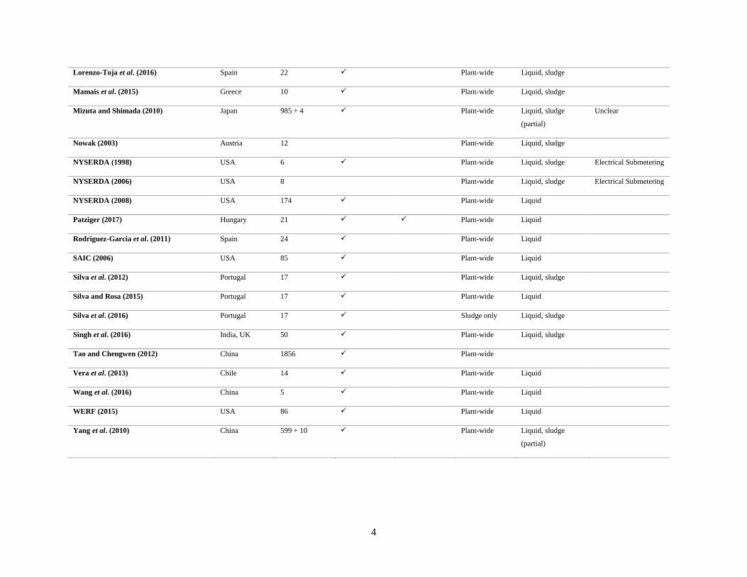
The literature was reviewed with the goal of identifying key aspects of prior studies that addressed

wastewater treatment benchmarking (Tables 2-1 and 2-2). Of the 37 studies, only two (Bailey et al., 2014;

Silva et al., 2016) solely examined sludge handling operations. The remaining studies employed

benchmarking metrics to characterize the entire treatment facility. Less than half of the reports addressed

the sludge handling processes employed at the plants (Table 2-1) and only five included metrics specifically

related to sludge production or quality (Table 2-2). It is thus evident that, historically, benchmarking

operations have not placed emphasis on the sludge handling component of wastewater treatment, and in

many cases have excluded analysis of such operations entirely. Yet, sludge processing and its associated

management can account for upwards of 40% of the operational costs for a WWTP (Lindtner et al., 2008;

Haslinger et al., 2016), and any improvements to the efficiency and efficacy of treatment inputs and disposal

practices can therefore have a beneficial impact on the environmental and economic sustainability of the

entire operation. As such, it was determined that there is a clear need for additional studies that develop and

employ detailed benchmarking methodologies to assess sludge handling operations.

3

Table 2-1: Characteristics of wastewater benchmarking studies

Study (Year) Location Number of

WWTPs in

Sample

Small WWTPs

in Sample?

Only Small

WWTPs

Studied?

Evaluation

Boundary

Treatment Types

Noted

On-site

measurements

AECOM (2018) Canada 53 ✓

Plant-wide

AECOM (2012) Canada 35 ✓

Plant-wide Liquid

AMBI (2017) Canada 5 ✓

Plant-wide Liquid

Bailey et al. (2014) USA 8

Sludge only Sludge only

Balmer (2000) Several 5

Plant-wide Liquid, sludge

Balmer and Hellstrom (2012) Sweden 24 ✓


Belloir et al. (2015) England 2 ✓ ✓ Plant-wide Liquid, sludge Electrical Submetering

Benedetti et al. (2008) Belgium 29 ✓

Plant-wide Liquid

Bodik and Kubaska (2013) Slovakia 68 ✓


Carlson et al. (2007) USA 266 ✓ Plant-wide Liquid, sludge

de Haas et al. (2015) Australia 142 ✓


Foladori et al. (2015) Italy 5 ✓ ✓ Plant-wide Liquid, sludge Electrical Submetering

Gallego et al. (2008) Spain 13 ✓ ✓ Plant-wide Liquid, sludge Partial Submetering

Gu (2016) China 9 ✓

Plant-wide Liquid

Hanna et al. (2017) USA 95 ✓ ✓ Plant-wide Liquid, sludge

(partial)

Haslinger et al. (2016) Austria 104 ✓ Plant-wide Liquid, sludge

Krampe (2013) Australia 24 ✓


Lindtner et al. (2008) Austria 6


4

Lorenzo-Toja et al. (2016) Spain 22 ✓


Mamais et al. (2015) Greece 10 ✓


Mizuta and Shimada (2010) Japan 985 + 4 ✓


(partial)

Unclear

Nowak (2003) Austria 12


NYSERDA (1998) USA 6 ✓

Plant-wide Liquid, sludge Electrical Submetering

NYSERDA (2006) USA 8

Plant-wide Liquid, sludge Electrical Submetering

NYSERDA (2008) USA 174 ✓

Plant-wide Liquid

Patziger (2017) Hungary 21 ✓ ✓ Plant-wide Liquid

Rodriguez-Garcia et al. (2011) Spain 24 ✓

Plant-wide Liquid

SAIC (2006) USA 85 ✓

Plant-wide Liquid

Silva et al. (2012) Portugal 17 ✓


Silva and Rosa (2015) Portugal 17 ✓

Plant-wide Liquid

Silva et al. (2016) Portugal 17 ✓

Sludge only Liquid, sludge

Singh et al. (2016) India, UK 50 ✓


Tao and Chengwen (2012) China 1856 ✓

Plant-wide

Vera et al. (2013) Chile 14 ✓

Plant-wide Liquid

Wang et al. (2016) China 5 ✓

Plant-wide Liquid

WERF (2015) USA 86 ✓

Plant-wide Liquid

Yang et al. (2010) China 599 + 10 ✓


(partial)

5

Table 2-2: Inputs/outputs evaluated in wastewater benchmarking studies

Study (Year) Energy GHG Chemicals WWTP

Effluent

Quality

Contaminant

Removal Efficiency

Labour Sludge

Handling

Others

AECOM (2018) ✓

AECOM (2012) ✓

AMBI (2017) ✓

Economics

Bailey et al. (2014) Sludge Only

Sludge

Sludge Several Economics

Balmer (2000) ✓

✓

✓ Production Economics

Balmer and Hellstrom (2012) ✓

✓ ✓

✓ Production,

quality

Economics

Belloir et al. (2015) ✓ ✓

Benedetti et al. (2008) ✓

✓ ✓

Several

Bodik and Kubaska (2013) ✓

Carlson et al. (2007) ✓

de Haas et al. (2015) ✓

Foladori et al. (2015) WW, Sludge

Gallego et al. (2008) ✓ ✓

Quality (metals) LCA

Gu (2016) ✓ ✓

Hanna et al. (2017) ✓

Haslinger et al. (2016) ✓

Krampe (2013) ✓

Lindtner et al. (2008) ✓

6

Lorenzo-Toja et al. (2016) ✓ ✓

LCA

Mamais et al. (2015) ✓ ✓

Mizuta and Shimada (2010) ✓

Nowak (2003) ✓

NYSERDA (1998) WW, Sludge

NYSERDA (2006) WW, Sludge

NYSERDA (2008) ✓

Patziger (2017) ✓

✓ ✓

Rodriguez-Garcia et al. (2011) ✓ ✓

LCA,

Economics

SAIC (2006) ✓

Silva et al. (2012) ✓

Production, TS,

% Beneficial

Use

Several

Silva and Rosa (2015) ✓

Silva et al. (2016)

Several

Singh et al. (2016) ✓ ✓

Tao and Chengwen (2012) ✓

Vera et al. (2013) ✓

✓ ✓

Production

Wang et al. (2016) ✓ ✓

WERF (2015) ✓

Yang et al. (2010) ✓

7

Energy issues are a key element of sustainability assessments and hence the method of assessing energy

utilization in prior studies (Table 2-2) was of interest. It was found that in prior benchmarking exercises,

data-driven approaches using real plant data were common. This included multiple studies that developed

benchmarking models within a region using advanced statistical techniques (AWWARF, 2007; Hanna et

al., 2017; Mizuta and Shimada, 2010). However, the insights provided by this information were often

limited in that they only employed utility bills for the entire plant to determine electricity consumption, and

thus did not contain any information related to the performance of individual unit processes.

Four studies (Belloir et al., 2015, Foladori et al., 2015, NYSERDA, 1998, NYSERDA, 2006) reported

the gathering of on-site power draw measurements (submetering) on individual pieces of equipment. Of the

four studies, one (Belloir et al., 2015) only evaluated two plants and thus provided a limited sample for

benchmarking purposes, and two (NYSERDA 1998, 2006) were commissioned by the same organization

and performed in the same general geographical location (New York State). These studies revealed that

while the submetering exercise can be time and labour intensive, it can provide a greater amount of insight

into the performance of the individual unit processes employed. Thus, it provides a deeper level of

information to plant owners and operators that seek to target specific areas of their operation for

improvement. This benefit was evidenced in the NYSERDA (2006) investigation, which identified $6.4

million in savings (representing 15% of total operation costs) through their study. A detailed discussion of

the audit methodologies employed by all four studies, and their relevance to the present study, is presented

in section 2.2.2.

The current study has a focus on small WWTPs and hence the size of facilities evaluated in the

benchmarking analyses was of interest. It was found that all but five studies included small treatment plants

as part of their sample (Table 2-1), however only six studies focused solely on WWTPs with average flows

less than 12,000 m3/d or less than 20,000 PE. Notably, several studies found that small WWTPs generally

exhibited higher specific energy consumption than larger plants (Bodik and Kubaska, 2013; Mizuta and

Shimada, 2010; Yang et al., 2010; Silva and Rosa, 2015; Haslinger et al., 2016; Singh et al., 2016) since

the former do not benefit from the “economies of scale” that the larger facilities exhibit. For facilities in

smaller communities where resources (economic, labour, etc.) are limited, minor improvements to process

operation can have a beneficial impact on the sustainability of the operations. The relatively limited

numbers of reported studies on small WWTPs confirmed the need for additional studies in this area.

8

Table 2-3: Normalizing bases employed in wastewater benchmarking studies

Study (Year) Volume of WW treated WWTP Influent Load Liquid Contaminant Mass

Removed

Other

AECOM (2018) ML

AECOM (2012) ML

AMBI (2017) m3

Bailey et al. (2014)

dry tonne of biosolids

Balmer (2000)

PE (N)

ton TS (sludge chemicals)

Balmer and Hellstrom (2012)

PE (not specified)

Belloir et al. (2015) m3

Benedetti et al. (2008) m3 PE (BOD, TN)

Bodik and Kubaska (2013) m3

(kWh/flow)/BOD load

Carlson et al. (2007) MG

de Haas et al. (2015)

BOD

Foladori et al. (2015) m3 PE (COD) COD

Gallego et al. (2008)

PE ("organic load")

Gu (2016) m3

Hanna et al. (2017) m3

Haslinger et al. (2016) PE (COD)

Krampe (2013)

PE (BOD)

Lindtner et al. (2008)

PE (COD)

Lorenzo-Toja et al. (2016) m3

9

Mamais et al. (2015)

PE (not specified)

Mizuta and Shimada (2010) m3

Nowak (2003)

COD

NYSERDA (1998) MG

NYSERDA (2006) MG

BOD lb. TSS removed (sludge ops)

NYSERDA (2008) MG BOD

Patziger (2017)

COD COD, TN

Rodriguez-Garcia et al. (2011) m3

kg PO4 removed

SAIC (2006) MG PE (not specified) BOD

Silva et al. (2012) m3

Silva and Rosa (2015) m3

BOD, COD

Silva et al. (2016)

dry tonne of sludge

Singh et al. (2016) m3

Tao and Chengwen (2012) m3

COD

Vera et al. (2013)

PE (inhabitants*year.)

Wang et al. (2016) m3

COD, NH3-N

WERF (2015) MG BOD

Yang et al. (2010) m3

Composite

10

The selection of factors to consider in carrying out a benchmarking activity was identified as important

in designing the proposed research program. A review of the studies detailed in Table 2-2 reveals that

energy consumption was the only metric common to all studies [whether directly or through conversion to

life cycle assessment (LCA) impact factors], and over half of the studies evaluated only this input. Of the

non-energy benchmarking studies, four evaluated greenhouse gas (GHG) emission quantities, five

benchmarked plant effluent quality (four of which also documented contaminant removal rate), six

evaluated economic costs (e.g. labour, operating and maintenance), and four inventoried other inputs, such

as chemicals. Given that facilities often face site-specific challenges of varying importance, the lack of

comprehensive benchmarking investigations incorporating inputs and outputs beyond energy was identified

as a knowledge gap. Further study in this regard is proposed, since improvements to any of the measures

could benefit the environmental, economic, and social sustainability of operations.

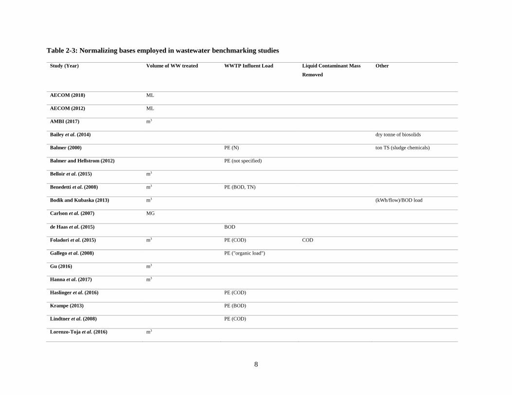
Benchmarking is typically conducted using normalized metrics that allow for comparisons between

facilities of differing scale. Of the 35 papers that evaluated plant-wide metrics, the most common

normalizing basis was “unit volume of wastewater treated” (24 papers), half of which solely benchmarked

on that basis (Table 2-3). While the easiest to obtain and calculate, thus making it the most convenient

option for studies involving a large number of facilities, exclusively benchmarking on a flow treated basis

can be limiting in that it does not account for the strength of the incoming wastewater, nor does it account

for differences in the goals of the treatment facility. For example, some facilities may require high inputs

to practice nutrient removal and meet stringent effluent quality targets; other plants may contain energy-

intensive sludge handling processes while exhibiting economical liquid treatment performance. Thus,

normalizing overall energy consumption (for example, through monthly electrical bills) by wastewater flow

can facilitate a high-level comparison between facilities of similar configuration but provides limited insight

into the performance of specific unit operations. Of the referenced studies, many (Table 2-1) did note the

general category of treatment for any given plant (and some detailed the specific treatment types), thereby

ensuring that the comparison between plants had some degree of “fairness”.

Other studies have included different normalizing bases with the goal of providing more insightful

comparisons and moving toward addressing the limitation identified. Eleven studies normalized their data

on the basis of influent contaminant mass loading [typically chemical or biochemical oxygen demand (COD

or BOD)], commonly expressed as a population equivalent (PE), of which four also included a flow-

normalized analysis. Such a basis provided a measure of the strength of incoming wastewater, although

only normalizing on organic load did not account for wastewaters that were high in nutrients (only two

studies based the PE on nitrogen load) and the methodology still lacked a measure for evaluating the

efficiency of the inputs in removing contaminants.

11

The inability to address efficiency in resource utilization has been identified as a deficiency and seven

studies normalized energy consumption by the extent of contaminant removal, in addition to flow and load

normalized analyses. The former metric was found to provide insight into the effectiveness of the inputs

(e.g. energy) as they relate to plant performance, which can help users identify opportunities of

improvement and process optimization. Studies by NYSERDA (2006) and SAIC (2006) have confirmed

the insightfulness of efficiency-based measures, as facilities were identified that, while performing better

than their peers on an overall energy consumption basis, exhibited lower energy efficiency than their peers.

Hence, it was concluded that opportunities for process improvement were likely present. Overall, it was

concluded that investigations which incorporate both flow/loading and efficiency-based metrics can

provide a greater level of insight into the systems of interest. The limited number of reports of benchmarking

studies that have incorporated such analysis, suggests a knowledge gap and area of need for future study.

In summary, while benchmarking of wastewater treatment operations is not a novel practice, there has

been a distinct lack of investigations into the following:

1. Benchmarking dedicated exclusively to sludge handling operations;

2. Benchmarking dedicated exclusively to small WWTP operations;

3. Detailed plant audits that feature on-site data collection of individual unit processes;

4. Benchmarking that extends beyond energy consumption to include all system inputs/outputs;

5. Methodologies that incorporate both quantity/composition of material treated and the

efficiency of inputs as normalizing bases for evaluation and comparison between samples.

2.2 Detailed Analysis of Relevant Benchmarking Studies

A closer examination of the benchmarking studies that were particularly relevant to the present study

was conducted to determine whether elements of the approaches employed previously could be

incorporated into the current study. This review included two studies focused solely on sludge handling

operations (section 2.2.1), and four studies that involved detailed energy audits with electrical submetering

(2.2.2).

2.2.1 Sludge handling Benchmarking Studies

Bailey et al. (2014) benchmarked the sludge handling performance of three WWTPs (and two water

treatment plants) in North Carolina with six comparable facilities within the United States. The additional

plants were selected because they had similar features to the North Carolina plants: separate biosolids

12

processing facilities with biosolids conveyance, a Class A EQ biosolids product, similar quantity of

biosolids production, regional handling, and similar equipment and processes (as an optional requirement).

To assess the facilities, a variety of benchmarking metrics were evaluated: labour (full time equivalents

and cost), power [kilowatt hour (kWh) consumption and cost], chemical costs, total combined operating

and maintenance costs, and final product cost and revenue on a dry tonne of biosolids produced basis.

Notably, the normalizing basis of biosolids production (end product) had the same limitation as the

wastewater flow/loading functional unit noted in the previous section: it did not account for the efficiency

of the inputs as they related to process performance. When compared to an alternative, one process may

have had a higher power draw on a biosolids produced basis, but a lower draw when related to quantity of

volatile solids destruction. It would therefore have been more insightful to include bases of both raw sludge

mass production and, for the stabilization step, quantity of volatile solids destruction.

Silva et al. (2016) also focused solely on evaluating WWTP sludge handling performance in a study

that extended from a prior WWTP performance assessment (Silva et al., 2012; Silva and Rosa, 2015). A

list of performance indicators and indices that covered a range of aspects related to sludge handling was

developed and evaluated for 17 WWTPs in Portugal. The metrics included quantity of sludge produced (per

volume of wastewater treated, and per mass of BOD and COD removal), percentage of sludge used

beneficially, quality compliance of sludge used in agriculture (binary compliant/non-compliant basis for

each required parameter), percentage of phosphorus (P) reclaimed (i.e. through beneficial use), and sludge

processing and disposal costs (both on a volume of treated wastewater basis and as a percentage of total

operating costs). The sludge processing cost measures were partitioned into those associated with energy

consumption and chemical use.

Some of the indicators in the Silva study provided insight into the sustainability of operations. These

included the percentage of sludge used for beneficial purposes, percentage of P reclaimed, and quality

compliance of the sludge used for agriculture. However, with respect to the latter indicator, simply reporting

a composite binary metric of compliance/non-compliance was limited in that it did not give an indication

of how close to the regulatory threshold any given parameter was. Thus, the consequence of a change in

regulations to more stringent contaminant limits was not obtained. Further, the wastewater volume basis

employed may be problematic since facilities that have higher sludge yields (for example, due to chemical

sludge production) could receive a disproportionately unfavourable result when compared to those with

lower sludge yields.

In summary, the benchmarking studies that have focused exclusively on sludge handling operations

have been limited in scope and rigour. Neither study employed rigorous energy or process audits, nor did

they comprehensively evaluate all the inputs and outputs of the systems being studied. The study of Silva

13

et al. (2016) incorporated several metrics that could be insightful from a sustainability assessment

perspective, but ultimately a need for a systematic methodology to comprehensively evaluate such systems

remains.

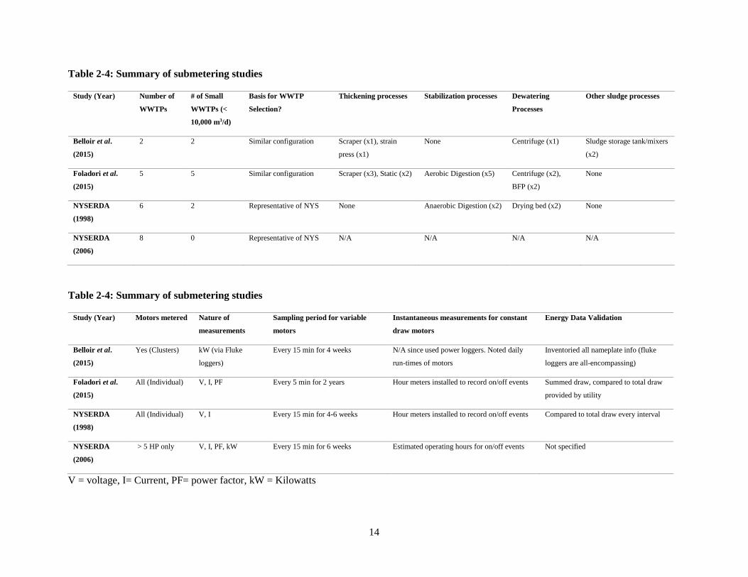
2.2.2 Benchmarking Studies Involving Energy Audits

Detailed audits that included electrical submetering of process equipment were of interest as it was

believed that they provide the most complete and accurate comparisons between peer facilities. The four

papers featuring detailed plant audits were therefore examined to determine whether elements of the

methodologies employed would be applicable to the current study. A summary of the key characteristics of

the relevant studies is shown in Table 2-4.

Among the four studies, there was broad agreement in the basic set-up of an energy audit. For motors

that had a constant power draw, single instantaneous measurements coupled with motor run-times (either

through installation of hour-meters, evaluation of plant records, or discussion with plant operators) were

employed to calculate the daily energy consumption. For motors that were equipped with variable frequency

drives (VFDs) or were otherwise manually adjusted based on process conditions (load, flow, etc.)

equipment that continuously measured the draw over a set period (typically 4-6 weeks) was installed to

capture the hourly and daily variations in demand.

Differences were observed with respect to the nature of energy-related measurements taken and the

corresponding method of energy data validation. Of the three parameters required for a power calculation

[voltage, current, and power factor (PF)], the NYSERDA (1998) study only directly measured the former

two parameters and the method for estimating the PF was not explicitly stated. The omission of direct

measurements of the PF likely resulted in an error in the power estimates as evidenced by the observations

that the sum of the sub-metered equipment draws represented only 61-93 percent of the total plant draw.

The authors indicated that the discrepancy was due to miscellaneous draws not captured by the submetering

equipment. However, given that the metered equipment included all motors, the discrepancy was likely

due to sources beyond miscellaneous draws such as errors in the PF values.

Two of the studies (NYSERDA, 2006; Foladori et al., 2015) measured single phase current, voltage,

and power factor (PF) separately, and then calculated the power draw (kW). The approach did not recognize

that the WWTPs typically employ three-phase electricity and that the phases may not be aligned, thereby

reducing the accuracy of the power draw estimates. In the Foladori et al. study, the data validation method

involved comparing the summed sub-metered draw to the total provided by the utility and was found to

occasionally yield differences of more than 10%. Only measured values that were less than this threshold

were included in the final analysis and thus the study did not make use of all available data.

14

Table 2-4: Summary of submetering studies

Study (Year) Number of

WWTPs

# of Small

WWTPs (<

10,000 m3/d)

Basis for WWTP

Selection?

Thickening processes Stabilization processes Dewatering

Processes

Other sludge processes

Belloir et al.

(2015)

2 2 Similar configuration Scraper (x1), strain

press (x1)

None Centrifuge (x1) Sludge storage tank/mixers

(x2)

Foladori et al.

(2015)

5 5 Similar configuration Scraper (x3), Static (x2) Aerobic Digestion (x5) Centrifuge (x2),

BFP (x2)

None

NYSERDA

(1998)

6 2 Representative of NYS None Anaerobic Digestion (x2) Drying bed (x2) None

NYSERDA

(2006)

8 0 Representative of NYS N/A N/A N/A N/A

Table 2-4: Summary of submetering studies

Study (Year) Motors metered Nature of

measurements

Sampling period for variable

motors

Instantaneous measurements for constant

draw motors

Energy Data Validation

Belloir et al.

(2015)

Yes (Clusters) kW (via Fluke

loggers)

Every 15 min for 4 weeks N/A since used power loggers. Noted daily

run-times of motors

Inventoried all nameplate info (fluke

loggers are all-encompassing)

Foladori et al.

(2015)

All (Individual) V, I, PF Every 5 min for 2 years Hour meters installed to record on/off events Summed draw, compared to total draw

provided by utility

NYSERDA

(1998)

All (Individual) V, I Every 15 min for 4-6 weeks Hour meters installed to record on/off events Compared to total draw every interval

NYSERDA

(2006)

> 5 HP only V, I, PF, kW Every 15 min for 6 weeks Estimated operating hours for on/off events Not specified

V = voltage, I= Current, PF= power factor, kW = Kilowatts

15

The Belloir et al. study (2015) employed a Fluke™ 1735 power logger to measure the three-phase

power draw to obtain the most accurate measure of power consumption. However, this study only installed

power loggers on motor control centres that captured the draw of several motors at once. Hence, to allocate

the consumption of individual pieces of equipment, nameplate parameters were used to calculate the

theoretical draw of each motor. As a result, the actual draw measured (via Fluke™) was almost two-fold

greater than the individual measurement sums. From these results, it is clear that when performing an energy

audit, a three-phase monitoring should be employed to collect power draw data on every motor of interest,

and thus eliminate uncertainty resulting from motors operating outside their stated voltage and power factor.

This choice would be especially important for a study submetering only the sludge handling processes since

it would not be possible to compare to the total utility bills for validation.

The Foladori et al. (2015) investigation was deemed to be particularly insightful when developing the

methodology for the current study. It presented an energy audit methodology and detailed a case study of

five WWTPs in Italy. The study was particularly relevant in that all five plants studied were small (less

than 10,000 m3/d flow) and employed aerobic digestion, which is commonly employed in similarly sized

facilities in Ontario (Jin and Parker, 2017). Energy consumption was normalized for each treatment stage

based on the nature of its purpose. As examples, the volume (m3) of wastewater treated was employed for

hydraulic based stages (pumping, settling etc.), COD removal was employed for COD-based stages

(oxidation tanks), and PE was used for building stages (e.g. lighting). Notably, COD-removal was also used

as the normalizing basis for the sludge handling stages.

In this study, it was acknowledged that energy consumption depended on waste sludge flows and solids

content (i.e. the mass processed) but noted that these parameters were not readily available in the small

WWTPs studied. Hence, COD-removal was employed as a proxy for sludge production. However, the use

of COD-removal as an indicator was also found to be somewhat limiting. While it did provide an indicator

of biological sludge production, it did not account for chemical sludge production (from precipitation of

phosphorus removal chemicals) and the sludge derived from influent fixed suspended solids. Still, from a

broader perspective, the recognition that small WWTPs frequently lack key process information highlighted

a key driver for the current study. The results of this study reinforced the need for a systematic approach

to auditing small WWTPs using real plant data, particularly as it relates to sludge handling processes and

associated management.

The allocation of energy consumption amongst numerous unit processes was reported to be challenging.

Specifically, for some plants (exact number not given), one blower supplied air to both the liquid train

aeration basins and the digesters, yet the partitioning of the power draw between the two processes was not

16

reported. It was thus evident that should the same situation be encountered in the current study, additional

measures should be taken to address it.

Despite these limitations two important conclusions were derived from this study: 1) the observation

of low energy efficiency in aerobic stabilization stages, and 2) low specific energy consumption required

for mechanical dewatering. The former reinforced the need to further investigate such systems at a detailed

level, while the latter represented an interesting finding from a sustainability standpoint. It suggests that

implementation of dewatering, which generates a cake that requires substantially less trucking (and

therefore less fuel consumption) than liquid sludges could improve environmental sustainability. This

hypothesis was therefore further investigated in the current study.

The NYSERDA (1998, 2006) studies both included several plants that were selected to be

representative of the region of interest (New York state). This approach differed from that of Foladori et al.

and Belloir et al., where plants were chosen to have similar configurations. In the former case, plants were

selected to capture the range of facility size, geographic location, and treatment technologies. It was elected

to employ these criteria in the current study due to the diversity of treatment plant configurations in Ontario

(Jin and Parker, 2017).

In summary, it was observed that obtaining instantaneous measurements for constant draw motors

(coupled with run-times) is generally accepted for auditing purposes, while motors with VFDs should be

monitored over a representative period of time to capture the fluctuations in draw. Advanced power loggers

capable of recording 3-phase power systems were found to provide the most accurate energy measurements.

Overall, performing detailed energy audits with equipment submetering has proved to be a valuable exercise

in obtaining a deeper knowledge of the performance of individual processes and equipment within a

WWTP.

2.3 Sludge handling Sustainability Studies

As previously described, benchmarking studies can provide insight into several metrics that are

indicative of the sustainability of wastewater treatment. However, prior studies that have assessed the

sustainability of sludge handling systems (Table 2-5) were performed with different goals and did not

involve benchmarking components. Notably, none of the previous studies were conducted within Canada

(or North America), which highlights an additional need for such a study to be performed. Of the studies

that were conducted, the most common goal of such studies was to evaluate the impact of different sludge

processing and end-use scenarios on sustainability. The studies have been conducted on the basis of either

a single WWTP (either existing or hypothetical) or the cumulative production of several plants in a

geographic region, based on the typical sludge type(s), volume(s), and composition(s) generated at the plant

17

or within the region. Given that several studies were indeed based on a single hypothetical plant, further

investigations into the sustainability performance of actual facilities (using real plant data) was identified

as a need for future study.

Despite the differing objectives, it was found that there was broad agreement in the literature regarding

the approach to conducting such evaluations. The approach involves a systematic assessment framework

consistent with LCA practices that comprises the following core elements, per ISO standards (ISO 14040,

14044):

1. Selection of the system functional unit (FU), the normalizing basis (i.e. denominator) for each

sustainability metric, that permits a standardized comparison between different options/scenarios;

2. Definition of system boundaries, which represent the system limits from which analysis will

incorporate inputs and outputs;

3. Selection of LCA impact categories, the sustainability metrics to be evaluated for each system input

and output;

4. Inventory of all relevant system inputs and outputs and conversion to selected LCA impact factors.

From Table 2-5 it can be seen that mass of sludge processed (dry weight basis) has most often been

selected as the FU from which to evaluate such systems (17 of 25 studies). This quantity directly represents

the quantity of material being processed, regardless of wastewater volume treated or COD load to the

WWTP.

There was broad agreement among the literature regarding the boundaries that should be employed for

such systems. Most studies included inputs and outputs related to the operation (i.e. processing/treatment),

transport, and disposal of the sludge/biosolids. Some investigations also included the infrastructure

construction phase in the analysis. However, multiple studies (Emmerson, 1995; Suh and Rousseaux, 2002)

have shown that over the lifespan of such infrastructure, the impact of construction is negligible when

compared to the cumulative impacts of continuous operation.

Among the LCA impact categories selected for evaluation, global warming potential (GWP) was the

only selection common to each study. Fewer studies evaluated other categories, including acidification,

eutrophication, human toxicity, and ecotoxicity potential. A variety of tools, typically a combination of

LCA software packages, databases, literature values, and available models were employed to convert the

inventoried inputs/outputs of each system to the desired impact category quantity. Such conversion

calculations require knowledge or assumption of a pathway from any given LCA input (e.g. electricity

production) to the impact category quantity.

18

Table 2-5: Summary of sludge handling sustainability studies

Author (Year) Location Goal of Evaluation Number of WWTPs Existing /

Hypothetical WWTP

Alayna et al. (2015) Australia Sludge processing/disposal scenarios 2 Existing

Alvarez-Gaitan et al. (2016) Spain 1 Existing

Barber (2008) Australia Sludge processing options with and w/o AD 1 Hypothetical

Beavis (2003) Poland LCA impact of converting from aerobic digestion to AD 1 Existing

Bridle and Skrypski-Mantele (2000) UK Sludge processing/disposal scenarios 1 Hypothetical

Chai et al. (2015) USA Wastewater treatment & sludge processing options 1 Hypothetical

Gallego et al. (2008) Sweden LCA benchmarking 13 Existing

Hara and Mino (2008) Denmark Sludge processing/disposal scenarios 12 (cumulative) Existing

Hong et al. (2008) Australia Sludge processing/disposal scenarios 1 Hypothetical

Hospido et al. (2005) Germany Processing/disposal scenarios - AD vs thermal processes 1 Existing

Houillon and Jolliet (2005) China Sludge processing/disposal scenarios 1 Hypothetical

Johansson et al. (2008) Spain Sludge disposal options 1 Existing

Li et al. (2013) Japan Sludge processing/disposal scenarios 1 Hypothetical

Liu et al. (2013) Japan Sludge processing/disposal scenarios 1 Hypothetical

Lundin et al. (2004) Australia Sludge processing/disposal scenarios 1 Existing

Lorenzo-Toja et al. (2016) Spain LCA benchmarking 22 Existing

Murray et al. (2008) Spain Sludge processing/disposal scenarios 4 (cumulative) Existing

Niu et al. (2013) China Sludge processing/disposal scenarios 1 Hypothetical

Peters and Lundie (2002) Sweden Sludge processing/disposal scenarios 3 (cumulative) Existing

Poulsen and Hansen (2002) China Sludge processing/disposal scenarios 2 (cumulative) Existing

19

Remy et al. (2013) Switzerland Sludge processing/disposal scenarios 1 Existing

Rodriguez-Garcia et al. (2011) China LCA benchmarking 24 Existing

Stefaniak et al. (2014) China Sludge processing/disposal scenarios 1 Hypothetical

Svanstrom et al. (2005) Sweden Sludge processing/disposal scenarios 1 Existing

Xu et al. (2014) China Sludge processing/disposal scenarios 1 Hypothetical

Table 2-5: Summary of sludge handling sustainability studies

Author (Year) Functional Unit System Boundaries LCA impact categories evaluated Energy

inventory

Chemicals

inventory

Metal

emissions

inventory

Nutrients

Inventory

Alayna et al. (2015) dry mass O, T, EU/D GWP ✓ ✓ ✓ ✓

Alvarez-Gaitan et al.

(2016)

Vol treated O, T, EU/D GWP, EP ✓ ✓ ✓

Barber (2008) dry mass O, T, EU/D GWP ✓ ✓

✓

Beavis (2003) dry mass O, T, EU/D GWP, energy ✓ ✓

✓

Bridle and Skrypski-

Mantele (2000)

dry mass O, T, EU/D GWP ✓ ✓ ✓

Chai et al. (2015) dry mass O, T, EU/D GWP, HTP, ETP, TETP, ADP, CED, TA,

FEP, MEP

✓ ✓ Unclear

Gallego et al. (2008) dry mass O, T, EU/D GWP, AP, EP, finite resource depletion ✓ ✓ ✓ ✓

Hara and Mino

(2008)

COD load to WWTP O, T, EU/D GWP, non-renewable resource depletion, LU ✓

Hong et al. (2008) dry mass C, O, T, EU/D GWP, HTP, energy ✓ ✓ ✓

Hospido et al. (2005) PE (COD load to

WWTP basis)

O, T, EU/D GWP, CED ✓ ✓ ✓ ✓

20

Houillon and Jolliet

(2005)

Vol of treated WW C, O, T, EU/D GWP ✓ ✓ ✓

Johansson et al.

(2008)

PE ("organic load") O, T, EU/D GWP, EP, TETP, AP, ADP, POFP, ODP ✓ ✓ ✓ ✓

Li et al. (2013) dry mass O, T, EU/D N/A ✓ ✓ ✓

Liu et al. (2013) dry mass C, O, T, EU/D GWP, AP, HTP, LU ✓ ✓ ✓

Lundin et al. (2004) Vol of treated WW O, T, EU/D GWP, CED, MEP, POFP, AP, HTP, TETP,

FAETP, MAETP

✓ ✓ ✓ ✓

Lorenzo-Toja et al.

(2016)

Vol treated, kg PO4

removed

O, T, EU/D GWP, EP ✓ ✓

Murray et al. (2008) dry mass O, T, EU/D GWP, EP, ODP, AP, POFP, ADP, HTP ✓ ✓ ✓

Niu et al. (2013) wet mass O, T, EU/D GWP ✓ ✓

Peters and Lundie

(2002)

dry mass O, T, EU/D GWP, AP, EP, resource depletion ✓ ✓ ✓

Poulsen and Hansen

(2002)

dry mass O, T, EU/D GWP ✓ ✓

Remy et al. (2013) dry mass C, O, T, EU/D GWP, NRE ✓ ✓ ✓

Rodriguez-Garcia et

al. (2011)

dry mass O, T, EU/D GWP, ODP, HTP, POFP, PMF, IR, TA,

FEP, MEP, TETP, FAETP, MAETP, LU,

ADP

✓ ✓ ✓

Stefaniak et al. (2014) dry mass O, T, EU/D GWP ✓ ✓ ✓

Svanstrom et al.

(2005)

dry mass T, EU/D GWP, AP, EP, FRU ✓ ✓ ✓

Xu et al. (2014) dry mass O, T, EU/D GWP, energy, AP ✓ ✓ ✓

O = operation phase, T = transport phase, EU/D = end-use / disposition

21

With respect to the types of inputs/outputs inventoried within the respective system boundaries, from

Table 2-5 it can be seen that all investigations quantified energy inputs and most inventoried chemical use.

A smaller number of studies evaluated biosolids quality for the purposes of evaluating chemical fertilizer

production offsets, and only nine studies evaluated heavy metal content of the biosolids product. Given that

the nutrient and heavy metal content of a biosolids product partially dictates the type of end-use that can be

employed, it is notable that studies to date have sometimes ignored such parameters, and the lack of

documentation represents a knowledge gap and area of need for further study.

In summary, sustainability studies that incorporate all of the goals and objectives of the current study

(i.e. a hybrid of benchmarking, energy/process audit, and sustainability) were not identified. However, the

following methodological elements that have been consistently employed in sludge handling sustainability

studies were identified as being relevant to the current study:

1. Employment of dry weight of sludge produced as the FU basis;

2. System boundaries drawn around the operation, transport and disposal phases of sludge

management;

3. At a minimum, GWP evaluated as the primary LCA impact category.

22

Chapter 3

Methodology

To achieve the goal of documenting the current sludge handling performance of small WWTPs in

Ontario, a methodology was developed to systematically evaluate the systems within a

benchmarking/sustainability framework using existing plant data and on-site measurements. Whenever

possible, the approach involved employing methodological elements that were consistent with those

established in the literature (Chapter 2), and when necessary were further refined and tailored to meet the

specific objectives of the study. The study can be broadly characterized into three components:

1. Selection of ten facilities for in-depth evaluation;

2. Development and implementation of a plant audit methodology, including selection of

benchmarking metrics;

3. Innovative technology assessment.

3.1 Plant Selection

For the purposes of the study, a “small” plant was defined as one with a design hydraulic capacity of

less than 10,000 m3/day that does not employ anaerobic digestion. Only mechanical treatment systems

(liquid train and sludge stabilization) were considered for evaluation; lagoon systems were excluded as

sludge generation at these facilities is sporadic. However, if a mechanical plant incorporated a lagoon as

part of its non-stabilization sludge handling process (e.g. for storage), it was still considered for selection.

To identify the facilities that met the initial screening criteria and would thus form the population of

plants from which selections would be made, an Ontario Ministry of the Environment and Climate Change

(MOECC) database containing basic plant information (location, hydraulic capacity, operator type, sludge

treatment processes, disposition practice) of all facilities province-wide was analyzed. However, as the

database was somewhat dated and incomplete in some areas, additional data were gathered on plants with

hydraulic capacity greater than 1000 m3/d to increase accuracy and completeness. The additional data

gathering involved contacting municipalities directly and obtaining information from municipal websites.

In total, 210 facilities met the initial screening criteria.

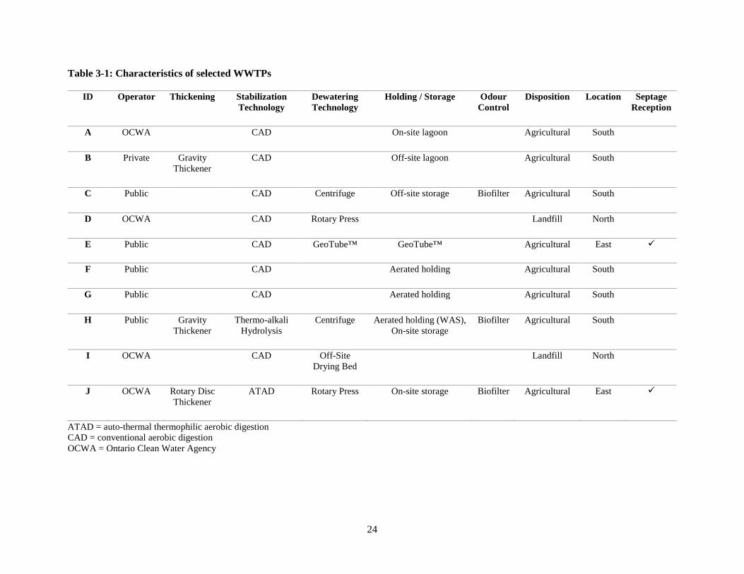
From the 210 plants that met the initial screening criteria, ten were selected (Table 3-1) to capture a

range of on-site sludge processing technologies (thickening, stabilization, dewatering), disposition practices

(land application, landfill), operator type [public, private, Ontario Clean Water Agency (OCWA)],

geographical locations (Southern, Eastern, Northern Ontario), and septage reception (present/not-present).

23

Although most small facilities in the province are not currently using an “innovative” technology (e.g.

thermo-alkali hydrolysis, GeoTube™, etc.) (Jin and Parker, 2017), it was considered important to have such

plants represented in the study to assess the extent to which newer technologies may impact the

sustainability of operations, and provide baseline knowledge for other communities considering upgrades

to or replacements of their existing process. Furthermore, although technologies such as centrifuge and

rotary press dewatering are reasonably well-established among large WWTPs, they are not as common in

small treatment facilities (Metcalf & Eddy, 2013) and thus would represent an innovation within the context

of small plants. Facilities that employed these technologies were thus included in the current ten plant

sample.

3.2 Audit Methodology

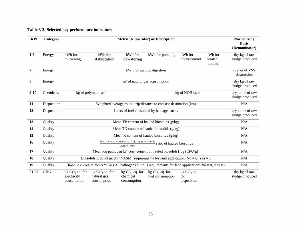
A variety of key performance indicators (KPIs) were established (Table 3-2) that could be broadly

categorized into energy consumption, chemical use, biosolids disposition, biosolids quality, and GHG

emissions. The first four categories were selected to represent all the operational inputs and outputs of the

systems studied, and to provide operational benchmarks for utilities seeking to quantify their individual

plant performance relative to others of similar scale and scope of operation. The last category was selected

as a means to cumulatively evaluate all previous categories on a common measure of environmental

sustainability: the carbon footprint.

Different energy sources (electricity, natural gas, transportation fuel) and chemicals have different

carbon emission debits associated with their respective production. Conversely, the land application of

biosolids reduces chemical fertilizer requirements and thus provides the sludge handling system with carbon

credits. Taken collectively, a metric that converted all the inputs to a single net carbon footprint was used

to evaluate the magnitude of environmental impact for each system.

Where appropriate, the KPIs were normalized on the basis of raw sludge (dry mass) produced, defined

as the mass of sludge entering the sludge handling process (from primary/secondary clarifiers) minus any

mass quantities in return streams (e.g. digester decant and centrifuge centrate). The mass flows in the return

streams were accounted for to ensure that facilities wasting large quantities of sludge did not receive a

disproportionately favourable result if they were also returning high quantities back to the liquid stream,

and thus had lower net sludge production than was apparent.

24

Table 3-1: Characteristics of selected WWTPs

ID Operator Thickening Stabilization

Technology

Dewatering

Technology

Holding / Storage Odour

Control

Disposition Location Septage

Reception

A OCWA CAD On-site lagoon Agricultural South

B Private Gravity

Thickener

CAD Off-site lagoon Agricultural South

C Public CAD Centrifuge Off-site storage Biofilter Agricultural South

D OCWA CAD Rotary Press Landfill North

E Public CAD GeoTube™ GeoTube™ Agricultural East ✓

F Public CAD Aerated holding Agricultural South

G Public CAD Aerated holding Agricultural South

H Public Gravity

Thickener

Thermo-alkali

Hydrolysis

Centrifuge Aerated holding (WAS),

On-site storage

Biofilter Agricultural South

I OCWA CAD Off-Site

Drying Bed

Landfill North

J OCWA Rotary Disc

Thickener

ATAD Rotary Press On-site storage Biofilter Agricultural East ✓

ATAD = auto-thermal thermophilic aerobic digestion

CAD = conventional aerobic digestion

OCWA = Ontario Clean Water Agency

25

Table 3-2: Selected key performance indicators

KPI Category Metric (Numerator) or Description Normalizing

Basis

(Denominator)

1-6 Energy kWh for

thickening kWh for

stabilization kWh for

dewatering kWh for pumping kWh for

odour control kWh for

aerated

holding

dry kg of raw

sludge produced

7 Energy kWh for aerobic digestion dry kg of VSS

destruction

8 Energy m3 of natural gas consumption dry kg of raw

sludge produced

9-10 Chemicals kg of polymer used kg of KOH used dry tonne of raw

sludge produced

11 Disposition Weighted average round-trip distance to end-use destination (km) N/A

12 Disposition Liters of fuel consumed by haulage trucks dry tonne of raw

sludge produced

13 Quality Mean TP content of hauled biosolids (g/kg) N/A

14 Quality Mean TN content of hauled biosolids (g/kg) N/A

15 Quality Mean K content of hauled biosolids (g/kg) N/A

16 Quality 𝑀𝑒𝑎𝑛 𝑚𝑒𝑡𝑎𝑙 𝑐𝑜𝑛𝑐𝑒𝑛𝑡𝑟𝑎𝑡𝑖𝑜𝑛,𝑑𝑟𝑦 𝑚𝑎𝑠𝑠 𝑏𝑎𝑠𝑖𝑠

𝑁𝐴𝑆𝑀 𝑙𝑖𝑚𝑖𝑡 ratio of hauled biosolids N/A

17 Quality Mean log pathogen (E. coli) content of hauled biosolids [log (CFU/g)] N/A

18 Quality Biosolids product meets “NASM” requirements for land application: No = 0, Yes = 1 N/A

19 Quality Biosolids product meets “Class A” pathogen (E. coli) requirements for land application: No = 0, Yes = 1 N/A

21-25 GHG kg CO2 eq. for

electricity

consumption

kg CO2 eq. for

natural gas

consumption

kg CO2 eq. for

chemical

consumption

kg CO2 eq. for

fuel consumption kg CO2 eq.

for

disposition

dry kg of raw

sludge produced

26

A BioWin™ model was generated for each plant to obtain a solids mass balance for the sludge handling

process, estimate net sludge production, and screen for problematic data. The modelling exercise involved

initial configuration to reflect reported operating conditions [influent/effluent characteristics, flows

(influent, waste/return sludge), chemical addition(s)] based on three years of historical operational data

(2014 – 2016, if available). Unknown return streams (e.g. digester decant, dewatering centrate) were then

adjusted such that the predicted aeration basin mixed-liquor suspended solids (MLSS) matched the reported

values and predicted biosolids quantities matched the reported amounts (if available).

3.2.1 KPI Category 1: Energy Consumption

For all but one of the plants studied, electricity was the only form of energy consumed. Several of the

energy KPIs thus involved normalized electricity consumption (kWh per dry kg of raw sludge) for the

sludge handling process. Individual electricity consumption KPIs for each stage of the sludge treatment

process (thickening, stabilization, dewatering, holding), odour control, and pumping were selected to ensure

information was obtained for each individual unit process. Additionally, recognizing that nine of the ten

plants practiced some form of aerobic digestion, an additional indicator was selected to relate digester

electricity consumption to the quantity of volatile solids reduction. The metric was selected to obtain a

measure of the energy efficiency of the process. The quantity of solids destroyed was estimated from the

BioWin™ model of each plant.

To determine the power draw of the various processing equipment (blowers, pumps, dewatering units,

etc.), spot measurements were collected on-site using a Fluke™ 1735 power logger. Power draw was

assumed to be constant over time since no major pieces of equipment incorporated variable frequency

drives. Centrifuge back drives were the only exception, however, draw for these motors were found to only

represent 5% of the total draw for the dewatering unit. The variation in draw was therefore assumed to be

negligible. Electricity consumption (kWh) was estimated by multiplying daily equipment run-times

(obtained from plant records and discussions with plant operators) with measured power readings (kW).

In most cases, the facilities employed dedicated blowers for aerobic digesters and holding tanks. Hence,

power draw was directly allocated to the sludge handling process of interest from the measurements taken

on-site. However, there were some instances where the same blower supplied air to both digesters and

aeration basins (plants B, F, I, and J), or to both the digester and aerated holding tank (plant G). In the cases

of plants B, G, and J, information on the air flow to each vessel was obtained to determine the percentage

of air (and in turn, the proportion of electricity) supplied to the processes of interest.

27

Air flow information was not available for plant F. Hence, diffuser information and dissolved oxygen

(DO) concentrations were employed in the BioWin™ model to estimate air flows and the corresponding

allocation of power draw. Neither flow information nor diffuser information were available for plant I.

Therefore, the proportioning was estimated based on the percentage of volume present in the aerobic

digesters and the extended aeration basin. The need for these estimates introduced some uncertainty into

the estimated KPIs for these five plants.

An additional energy KPI reflected the use of natural gas at plant H. It was calculated by subtracting

the reported baseline usage (for plant-wide heating) from the total draw reported during stabilization

operation and dividing the difference by the dry mass flow of sludge processed.

3.2.2 KPI Category 2: Chemical Usage

While several of the facilities only used chemicals in the liquid train (for phosphorus removal), those

that practiced dewatering or mechanical thickening used polymer to enhance the liquid-solid separation

process. In addition, one of the facilities (plant H) used potassium-hydroxide (KOH) for pH control and to

boost the potassium content of the biosolids product. Two KPIs were selected to reflect these inputs.

Chemical usage information was obtained from plant records and/or conversations with plant operators.

However, the specific form in which the information was available was not consistent across all plants.

Specific usage quantities were calculated using reported chemical purchase records (plant C),

barrels/volumes consumed per month (plants D and J), dosing rates (plants E), and flow rates (plant H).

3.2.3 KPI Category 3: Biosolids Disposition

Separate indicators that employed the average distance that the biosolids travelled to their destination

and the amount of fuel consumed (normalized to dry mass of solids processed) were created. The latter

indicator was chosen to account for the variety in capacity and fuel economy of the trucks in use. Liquid

biosolids are typically transported in large tanker trucks with capacities of approximately 40 m3 per truck,

while dewatered cake is often hauled in small-to-medium sized dump trucks that have smaller capacities

and lower fuel requirements.

Biosolids disposition information [quantities and farm/landfill address(es)] was obtained from haulage

reports and Google Maps™ was employed to determine the shortest driving distance from the WWTP to

each destination. To calculate the normalized fuel consumption of each operation, the distance value was

used in conjunction with truck fuel economy information obtained from the truck owner.

28

3.2.4 KPI Category 4: Biosolids Quality

Biosolids contain nutrients [phosphorus (P), nitrogen (N), potassium (K)] that are beneficial for

agricultural crop growth, but also contain heavy metals and pathogens that can be harmful to human health

at high concentrations. Limits for the latter two measures have been established in the Nutrient Management

Act for Non-Agricultural Source Material (NASM) application (O. Reg. 267/03 – Schedule 5 and 6, CM2

and CP2). Further distinctions regarding pathogen content are stipulated under the US EPA regulatory

framework (US EPA, 1993). Under EPA guidelines, a “Class A” product must contain less than 1000

MPN/g of E. coli, while a “Class B” product must have less than 2x106 CFU/g (US EPA, 1993). The latter

value is consistent with the NASM requirement in Ontario (O. Reg. 267/03 – Schedule 5, CM2). In Canada,

if a biosolids product meets thresholds for pathogen content, it can qualify as a CFIA-certified fertilizer

under the Fertilizers Act (R.S.C., 1985, c. F-10) and associated Fertilizers Regulations (C.R.C., c. 666).

KPIs for mean nutrient and log-mean E. coli concentrations were selected to identify the range of

beneficial value (nutrients) and proximity to the NASM pathogen limit (E. coli) of the hauled biosolids. In

addition, a KPI relating the highest ratio of mean metal concentration to its respective NASM limit was

selected to determine whether any metals were at risk of exceeding regulatory thresholds. In addition, binary

indicators were included to represent whether the biosolids were a) meeting NASM requirements for land

application, and b) meeting E. coli requirements for classification as a Class A product. Quality data was

obtained from plant records for eight of the ten plants practicing land application of biosolids. For the two

plants landfilling their biosolids, such information was not available. To determine the quality

characteristics for the latter two plants, a sampling program was implemented to characterize the biosolids

product leaving the plant (cake and liquid for plants D and I, respectively). The sampling program involved

measuring all parameters of interest (nutrients, E. coli, metals) for four months on a bi-weekly basis. All

samples were collected by plant operators and sent to MOECC accredited labs for analysis.

3.2.5 KPI Category 5: Greenhouse Gas (GHG) Emissions

CO2 emissions were calculated for each facility on the basis of emission factors that were obtained from

the literature for each input and output. Where possible, emission factors specific to Ontario (electricity,

natural gas production) or Canada (transportation fuel) were employed. In other cases, literature values for

chemical production (polymer, KOH) and chemical fertilizer production (N, P, K) were utilized. The latter

factors were used to determine the carbon off-sets gained by using biosolids as a fertilizer through the

avoidance of chemical fertilizer production for each nutrient. The emission factors utilized are listed in

Table 3-3.

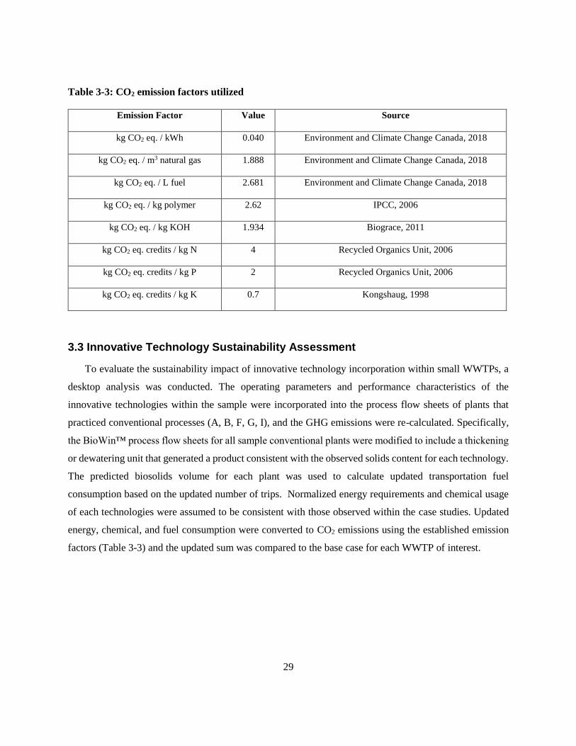
29

Table 3-3: CO2 emission factors utilized

Emission Factor Value Source

kg CO2 eq. / kWh 0.040 Environment and Climate Change Canada, 2018

kg CO2 eq. / m3 natural gas 1.888 Environment and Climate Change Canada, 2018

kg CO2 eq. / L fuel 2.681 Environment and Climate Change Canada, 2018

kg CO2 eq. / kg polymer 2.62 IPCC, 2006

kg CO2 eq. / kg KOH 1.934 Biograce, 2011

kg CO2 eq. credits / kg N 4 Recycled Organics Unit, 2006

kg CO2 eq. credits / kg P 2 Recycled Organics Unit, 2006

kg CO2 eq. credits / kg K 0.7 Kongshaug, 1998

3.3 Innovative Technology Sustainability Assessment

To evaluate the sustainability impact of innovative technology incorporation within small WWTPs, a

desktop analysis was conducted. The operating parameters and performance characteristics of the

innovative technologies within the sample were incorporated into the process flow sheets of plants that

practiced conventional processes (A, B, F, G, I), and the GHG emissions were re-calculated. Specifically,

the BioWin™ process flow sheets for all sample conventional plants were modified to include a thickening

or dewatering unit that generated a product consistent with the observed solids content for each technology.

The predicted biosolids volume for each plant was used to calculate updated transportation fuel

consumption based on the updated number of trips. Normalized energy requirements and chemical usage

of each technologies were assumed to be consistent with those observed within the case studies. Updated

energy, chemical, and fuel consumption were converted to CO2 emissions using the established emission

factors (Table 3-3) and the updated sum was compared to the base case for each WWTP of interest.

30

Chapter 4

Results

The benchmarking results associated with each system input and output were evaluated

(sections 4.1 - 4.5) and a desktop analysis of the impacts of innovative technology implementation into

plants with conventional process configurations was conducted (section 4.6). Where possible, uncertainties

in the estimated values (expressed as the standard deviation as a percentage of the mean for each KPI) were

calculated from the raw data set. Among the KPIs that involved raw sludge production, the variability in

production represented the largest source of uncertainty. The standard deviations associated with raw sludge

production were found to range from 11 – 34% of the mean values. The variability was attributed to

differences in biological activity (biomass growth), influent fixed suspended solids, and chemical sludge

production (if chemical addition for P-removal was practiced). There was also unquantifiable uncertainty

associated with a) parameter estimates provided by operators (e.g. polymer use), and b) partitioning of

electricity draw when one blower supplied air to both liquid stream aeration basins and digesters. These

qualitative uncertainties were described in the methodology section. Where necessary, the implications of

such uncertainties (quantitative and qualitative) on the extent to which conclusions may be drawn are

discussed in subsequent results sections.

4.1 Energy KPI Results

Energy inputs represent a portion of a treatment facility’s total operational costs and the GHG emissions

associated with their production represent an environmental impact. As such, reductions in this area without

compromising plant performance can potentially improve economic and environmental sustainability. The

following discussion details the KPIs related to electricity and natural gas consumption.

4.1.1 Electricity Consumption – Overall

All ten plants within the study consumed electricity as part of the sludge-treatment process. Total

electricity consumption with associated uncertainty for each facility is presented in Figure 4-1, while the

contributions of individual processes to total consumption is shown in Figure 4-2. As shown in Figure 4-1,

total consumption ranged from 0.9 – 3.9 kWh/dry kg of raw sludge among all plants studied. The 25th, 50th

and 75th percentile values corresponded to 1.8, 2.2, and 2.7 kWh/dry kg, respectively.

31

Figure 4-1: Total electricity consumption per dry mass of raw sludge produced

Figure 4-2: Total electricity consumption per dry mass of raw sludge produced (detailed)

0.0

0.5

1.0

1.5

2.0

2.5

3.0

3.5

4.0

4.5

Plant I Plant D Plant A Plant F Plant C Plant G Plant H Plant E Plant B Plant J

kWh

/ d

ry k

g

0

0.5

1

1.5

2

2.5

3

3.5

4

Plant I Plant D Plant A Plant F Plant C Plant G Plant H Plant E Plant B Plant J

kWh

/ d

ry k

g

Thickening Stabilization Dewatering Aerated Holding Odour Control Pumping

32

When incorporating quantitative uncertainty into the analysis, it can be seen from Figure 4-1 that there

was overlap in the uncertainty bars between all plants inclusive of the second (plant B) and eighth (plant A)

highest consumers. The considerable overlap indicated that total electricity consumption was similar for a

number of plants in the study. Notably, the lowest consumer (plant I) exhibited consumption that was

statistically different than the next closest consumer (plant D). However, as discussed in the methodology,

there was unquantified uncertainty in plant I estimates as it did not employ a dedicated digester blower.

Hence, the low KPI for plant I may not be a feasible goal for plants seeking to reduce electricity

consumption.

When the type of sludge handling technologies employed was considered, the facilities that did not

practice conventional aerobic digestion exhibited the highest (ATAD) and fourth-highest (thermo-alkali

hydrolysis) electricity consumption, respectively. The former facility consumed 44% more energy per unit

of raw sludge mass than the next highest consumer, indicating that the ATAD technology was substantially

more energy-intensive than the conventional aerobic digestion processes within the sample. Among the

eight plants practicing conventional aerobic digestion, total electricity consumption ranged from

0.9 – 2.7 kWh/dry kg. For such plants, the 25th, 50th and 75th percentile corresponded to 1.6, 2.0, and

2.4 kWh/dry kg, respectively.

Two facilities (E and J) that practiced septage reception were evaluated to assess the impacts of this

practice on KPI values. Septage is a partially stabilized material that directly contributes to sludge

production via fixed suspended solids loading (Metcalf & Eddy, 2013). It was expected that plant would

exhibit higher sludge production and aeration basin MLSS than predicted (modelled) values as the modeling

did not account for this input. Plant E exhibited a lower MLSS value than the simulated concentrations.

The facility also exhibited the highest uncertainty in raw sludge production (34%) among all plants studied.

In addition, plant E was operated at a higher solids retention time (SRT) than all other facilities studied.

Collectively, these factors contributed to the difficulty in ascertaining the impact of septage reception on

the energy consumption at the plant. Plant J was an ATAD facility that required substantially greater energy

input as a result of the chosen stabilization process, which resulted in difficulty extracting the energy

consumption due to septage reception. It did generate similar quantities of sludge to the predicted value,

which indicated that increased solids loading from septage was sufficiently represented by the BioWin™

model. Ultimately, no conclusions could be drawn regarding the impact of septage reception on sludge

handling energy requirements because both case studies exhibited additional factors that could not be de-

lineated from the reception of this material.

33

4.1.2 Electricity Consumption – Stabilization

As shown in Figure 4-2, the electricity allocated to stabilization represented the highest fraction of

sludge handling electricity consumed for all but two of the plants studied (F and H). With the exception of

these two plants, at least 82% of the electricity consumption in all of the facilities was used for stabilization.

The high proportion of electricity utilized for stabilization suggests that this process should generally be an

area of interest for plant owners and operators that seek to selectively target high usage unit processes within

their overall treatment system. A reduction of the electricity required for stabilization would have a greater

impact on total usage reduction than the same percent reduction achieved within other processes

(e.g. dewatering).

Normalized power consumption values for the stabilization processes alone (with associated

uncertainties) are shown in Figure 4-3. Among all the plants studied, electricity consumption for

stabilization ranged from 0.3 to 3.8 kWh/dry kg. The 25th, 50th and 75th percentile values corresponded to

1.0, 1.6, and 2.5 kWh/dry kg, respectively. However, the results differed from the overall consumption

results in that any given plant’s uncertainty bar in Figure 4-3 generally overlapped with fewer other plants

than those in the previous (overall) analysis. The most overlap any single plant exhibited in Figure 4-3 was

four facilities, whereas some facilities exhibited as many as six overlapping values in Figure 4-1. The

observation indicates that the ranking of consumers with respect to stabilization draw was more defined

than that of the overall ranking. Furthermore, given that all the plants employed the same technology, the

over two-fold increase in consumption between the 25th and 75th percentile indicates that opportunities for

process optimization in some of the higher consumers may exist.

The maximum consumption associated with stabilization corresponded to the facility that employed

ATAD, while the minimum value corresponded to the plant that employed thermo-alkali hydrolysis. The

latter plant’s uncertainty bars did not overlap with any other facility, which indicated that it was also the

best performer when quantitative uncertainty was incorporated into the analysis. The observation that

thermo-alkali hydrolysis was the lowest consumer for stabilization is noteworthy when considering the

technology’s application in other facilities. If the thermo-alkali hydrolysis process were to be implemented

at a plant that did not require aerated holding or odour control (the two largest power consumers for sludge

handling operations at plant H), the potential for electricity savings could be substantial relative to the

conventional aerobic digestion process.

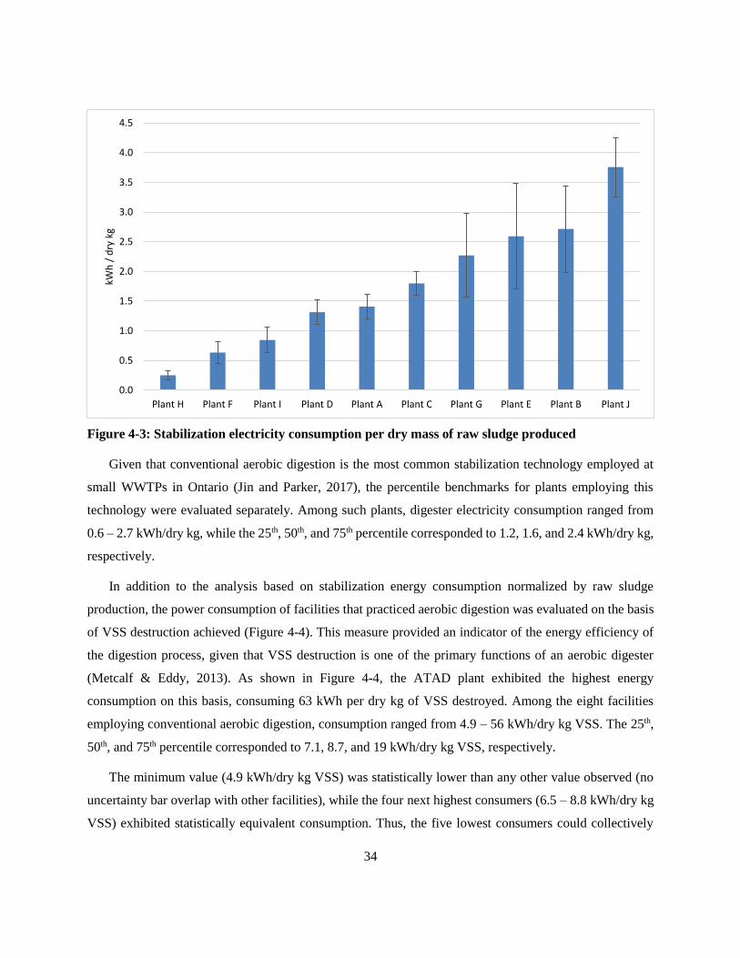
34

Figure 4-3: Stabilization electricity consumption per dry mass of raw sludge produced

Given that conventional aerobic digestion is the most common stabilization technology employed at

small WWTPs in Ontario (Jin and Parker, 2017), the percentile benchmarks for plants employing this

technology were evaluated separately. Among such plants, digester electricity consumption ranged from

0.6 – 2.7 kWh/dry kg, while the 25th, 50th, and 75th percentile corresponded to 1.2, 1.6, and 2.4 kWh/dry kg,

respectively.

In addition to the analysis based on stabilization energy consumption normalized by raw sludge

production, the power consumption of facilities that practiced aerobic digestion was evaluated on the basis

of VSS destruction achieved (Figure 4-4). This measure provided an indicator of the energy efficiency of

the digestion process, given that VSS destruction is one of the primary functions of an aerobic digester

(Metcalf & Eddy, 2013). As shown in Figure 4-4, the ATAD plant exhibited the highest energy

consumption on this basis, consuming 63 kWh per dry kg of VSS destroyed. Among the eight facilities

employing conventional aerobic digestion, consumption ranged from 4.9 – 56 kWh/dry kg VSS. The 25th,

50th, and 75th percentile corresponded to 7.1, 8.7, and 19 kWh/dry kg VSS, respectively.

The minimum value (4.9 kWh/dry kg VSS) was statistically lower than any other value observed (no

uncertainty bar overlap with other facilities), while the four next highest consumers (6.5 – 8.8 kWh/dry kg

VSS) exhibited statistically equivalent consumption. Thus, the five lowest consumers could collectively

0.0

0.5

1.0

1.5

2.0

2.5

3.0

3.5

4.0

4.5

Plant H Plant F Plant I Plant D Plant A Plant C Plant G Plant E Plant B Plant J

kWh

/ d

ry k

g

35

serve as benchmarks for other utilities seeking to determine their performance relative to peers of similar

scope and operation. The low consumption in plant C may have been due to the type of sludge being

digested. The facility generated a mix of primary and secondary sludge, the former of which is more readily

biodegradable than secondary sludge (Metcalf & Eddy, 2013). The resulting mixture thus generally requires

less air to achieve a given quantity of VSS destruction than pure secondary sludges (Metcalf & Eddy, 2013).

One other facility generated primary sludge (plant B) and exhibited the second lowest specific energy

consumption (uncertainty bar overlap with three facilities), despite being the second highest overall

consumer (Figure 4-1).

Figure 4-4: Digester electricity consumption per dry mass of VSS destruction

Plants G and E exhibited over three- and six- fold greater energy consumption than the median value,

respectively. Both facilities exhibited higher specific consumption than the next highest consumer (plant I)

even when considering the quantitative uncertainty associated with the raw sludge production (neither

plant’s uncertainty bar overlapped with plant I). To provide insight into why each facility exhibited notably

higher consumption, the hydraulic residence time (HRT) of each facility was examined and found to be 48

and 58 days HRT, respectively. Both values were substantially higher than the MOECC (2008) design

guideline of 15 days HRT, which suggests that both digesters are a) oversized based on the current loading

0

10

20

30

40

50

60

70

80

Plant C Plant D Plant A Plant B Plant F Plant I Plant G Plant E Plant J

kWh

/ d

ry k

g V

SS

36

to the digester, and/or b) have air requirements for mixing that exceed the air supply requirements for VSS

destruction. Essentially, both units are effectively operating as aerated holding tanks in addition to their

function as aerobic digesters.

The energy efficiency evaluation revealed that some of the facilities that performed best when evaluated

on a raw sludge production basis were among the worst performers when evaluated on the basis of VSS

destruction achieved, and vice versa. Among plants that practiced conventional aerobic digestion, plant I

exhibited the second lowest energy consumption when normalized by raw sludge production, but the third

highest consumption when normalized by VSS destruction achieved. Plant B exhibited the highest

consumption under the former basis, but a value less than the median when evaluated on the latter basis.

While plants G and E were among the highest consumers when normalized by raw sludge production, the

extent to which they were the highest consumers when normalized by VSS destruction was substantially

greater than when evaluated under the previous basis. As previously discussed, the digesters for both plants

G and E were likely oversized based on the current VSS loading, which contributed to the high specific

consumption observed.

Different bases of normalization provide opportunities to derive conclusions based on different aspects

of the operation. Normalizing by raw sludge production provides a measure of overall performance, while

normalizing by VSS destruction provides a measure of energy efficiency. The examination of energy

efficiency in stabilization provided insight into areas where improvement might be possible and highlighted

possible deficiencies that would not have been identified had energy consumption only been calculated on

a raw sludge production basis. Given the broad range of values observed, opportunities for improvement

from an energy efficiency basis may exist in several of the facilities studied.

4.1.3 Electricity Consumption – Dewatering

Dewatering is employed to convert liquid biosolids into a cake. Of the five plants that practiced

dewatering, four employed a mechanical process that required electricity as part of its operation. The fifth

plant employed a passive process (GeoTube™) that involved storing aerobically digested biosolids in large

geo-membrane bags. In this process, leachate seeps through the pores of the bags and the dried solids are

retained within the bag. Among plants with mechanical dewatering, the normalized power draw for

dewatering ranged from 0.06 – 0.10 kWh/dry kg (Figure 4-5). The minimum and maximum values

corresponded to centrifuge processes and did not exhibit overlap of the uncertainty bars (indicating

distinctly higher and lower consumption between the two samples). The two rotary presses consumed

between 0.07 – 0.09 kWh/dry kg, however, overlap between the uncertainty bars indicated that there was

37

no statistical difference between the two values. Notably, the percentage of total sludge handling electricity

consumed by the dewatering processes ranged from 2% (plants H and J) to 5% (plants C and D). The low

percentages of total sludge handling power draw indicated that the additional energy required to convert

liquid sludges into cake via mechanical dewatering was relatively minor.

Figure 4-5: Mechanical dewatering electricity consumption per dry mass of raw sludge produced

4.1.4 Electricity Consumption – Pumping

For all but one of the plants studied, pumping represented a minor percentage of the total sludge

handling draw (1 – 4 %). Among all plants studied, the 25th, 50th, and 75th percentile of pumping electricity

consumption corresponded to 0.02, 0.04, and 0.05 kWh/dry kg, respectively. Plant A represented an

extreme value in this regard where pumping represented 18% of the total draw. Its normalized consumption

was 0.30 kWh/dry kg, which was a three-fold greater consumption than the next highest consumer (0.10

kWh/dry kg). The identification of the cause for the high use was beyond the scope of the study, but a

possible explanation involved the solids content of the feed sludge. Specifically, the wasted secondary

sludge was dilute (~ 0.5% TSS), which may have resulted in increased pumping requirements to waste the

desired mass of sludge.

4.1.5 Electricity Consumption – Aerated Holding

Among the three plants that employed aerated holding of sludge, plants F and H exhibited similar

consumption for the process (1.34 and 1.27 kWh/dry kg, respectively), while plant G exhibited a

0.00

0.02

0.04

0.06

0.08

0.10

0.12

Plant H Plant D Plant J Plant C

kWh

/ d

ry k

g

38

substantially lower value (0.04 kWh/dry kg). Both plants F and H employed a dedicated blower for their

holding tank, while plant G utilized a portion of the air provided by its digester blower to aerate the holding

tank (the reported air flow to each unit was used to determine its corresponding allocation of electricity

consumption). The discrepancy in values may be explained by the observation that plant G employed an

extended HRT in its digester (48 days), which indicated that it was effectively employing its digester as a

holding tank.

4.1.6 Electricity Consumption – Odour Control

There was a broad range of electricity consumption values associated with odour control: plants J, C,

and H consumed 0.02, 0.13, and 0.98 kWh/dry kg, respectively. The underlying cause of the wide range

was beyond the scope of the study, however site-specific considerations likely influenced the quantity of

electricity required to eliminate odours. All three facilities employed biofilters to remove odours. However,

only the facility that practiced thermo-alkali hydrolysis (plant H) employed a highly engineered system and

this corresponded to the highest normalized power draw. Since plant H did not practice aerobic digestion

(which aids in odour removal), its odour control system would need to remove all the odours generated by

the sludge, which likely increased the energy input requirements. One would have expected the ATAD

system to require higher electricity requirements since ATADs have historically been associated with

considerable odour emissions (Metcalf & Eddy, 2013). However, the sample facility employed a relatively

new “second-generation” ATAD process which is substantially less odourous than early “first generation”

systems (Metcalf & Eddy, 2013). One could also hypothesize that the ATAD process required lower

volumes of air for treatment than the thermo-alkali hydrolysis process, thereby reducing the electricity

requirements for odour control.

4.1.7 Natural Gas Consumption

In the current study, one facility consumed natural gas as part of its sludge treatment process (plant H).

The observed consumption was 0.04 m3 natural gas/dry kg. The lack of natural gas usage within the study

sample suggests that it is not a common form of energy employed at small WWTPs for the purposes of

sludge processing. Indeed, anecdotal conversations with owners and operators revealed that natural gas was

typically only used to heat office buildings, if it was used at all.

4.2 Chemical Usage KPI Results

Chemical use is necessary to achieve the goals of some treatment processes. For all the thickening and

dewatering processes within the study, polymers were used to enhance the liquid-solid separation process.

39

In addition, KOH was employed as part of the stabilization process in one instance. The purchase of

chemicals represents an operational cost for plant owners and the GHG emissions associated with their

production represent an environmental burden.

For the plants within the study that employed thickening and/or dewatering processes, normalized

polymer usage and the corresponding biosolids cake total solids (TS) content are shown in Figure 4-6.

Among the selected plants, one plant (J) employed a thickening technology (rotary disc thickener), one

plant (E) employed a passive dewatering technology (GeoTube™), and four plants (C, D, J, H) employed

mechanical dewatering processes. Plants C and H employed centrifuges, while plants D and J employed

rotary presses.

Figure 4-6: Chemical usage per dry mass of raw sludge produced and biosolids TS content

The rotary disc thickener consumed 12 kg of polymer per dry tonne (dt) of raw sludge and generated a

4.5% TS sludge product. The GeoTube™ consumed 9 kg polymer/dt and generated a 9.2% TS product.

Polymer usage for rotary press operation ranged from 20 – 28 kg polymer/dt (no uncertainty bar overlap)

and generated a biosolids cake ranging from 16.9 – 18.4% TS (uncertainty bar overlap). Polymer usage for

centrifuge operation ranged from 8 – 24 kg polymer/dt (no uncertainty bar overlap) and generated a

biosolids cake ranging from 17.2 – 22.5% TS (no uncertainty bar overlap). Notably, the lower centrifuge

0

5

10

15

20

25

30

35

Plant C Plant E Plant D Plant H Plant J

Thickening kg polymer / dt Dewatering kg polymer / dt Biosolids TS (%)

40

chemical usage value corresponded to the higher TS content. The lower dosage was employed at the plant

that generated a mixed primary/secondary sludge, which typically exhibits higher dewaterability than pure

secondary sludges (Metcalf & Eddy, 2013).

Among the two rotary disc thickeners evaluated, the polymer usage and solids content extended beyond

the range of values reported in the literature. Rotary presses employed for dewatering aerobically digested

waste activated sludges have been reported to consume a maximum of 17.5 kg polymer/dt and achieve

28 – 45% solids (Metcalf & Eddy, 2013). For centrifuge use, literature indicates that 10 – 15 kg polymer/dt

can be employed to achieve between 18 – 25% solids (Metcalf & Eddy, 2013). The observed discrepancies

between observed and literature values may indicate that excess polymer was being dosed in some cases,

or that the polymers employed were less effective as coagulating/flocculating agents than those reported in

literature. Finally, although operational inputs were not converted into economic costs in the current study,

it is important to note that polymers can vary widely in price. It is therefore possible that the more effective

polymers were more expensive, which is an additional sustainability aspect for plant owners to consider.

In addition to polymer usage for dewatering, plant H utilized KOH as part of its stabilization process.

The observed usage was 19 kg KOH/dt. The relative impact of the KOH and polymer use at this plant on

GHG emissions will be detailed in section 4.5.

Overall, there was a broad range of chemical use employed at the facilities within the sample. Rotary

thickening and GeoTube™ dewatering generally consumed the least with 12 and 9 kg/dt, respectively.

Rotary press and centrifuge dewatering operations consumed 20 – 28 kg/dt and 8 – 24 kg/dt, respectively.

Three of the mechanical dewatering usage values were higher than those reported in literature. The

observation suggests that the polymers may have been overdosed in the sample cases, or that the chemicals

used were less effective as coagulants/flocculants than those reported in literature. One facility utilized

KOH as part of its stabilization process and consumed 19 kg KOH/dt.

4.3 Disposition KPI Results

The disposal of biosolids represents an operational cost for wastewater treatment plant owners, and the

carbon emissions associated with trucking fuel consumption represent an environmental burden.

Disposition KPIs involving the average distance that biosolids were hauled and the associated normalized

fuel consumption were evaluated (Figure 4-7). For the former calculation, uncertainty was assumed to be

constant (0.5 km) since Google Maps™ was employed to obtain the exact address of each farm/landfill and

uncertainty was therefore only associated with variation in distance travelled within a given farm.

41

Uncertainty for the fuel consumption was directly a result of the uncertainty in estimated raw sludge

production for each plant.

Figure 4-7: Disposition KPI results

From Figure 4-7 it can be seen that the average round-trip trucking distance ranged from 8 – 83 km.

There was a substantial difference in trucking distance requirements between the lower and upper five

facilities studied. Half of the plants required less than 16 km of round-trip trucking to dispose of their

biosolids, while the other half required more than 52 km. The three highest distances corresponded to plants

(C, B, I) that did not have on-site storage, which necessitated additional trucking. In each case, transport

involved trucking the biosolids from the WWTP to an off-site location (storage building, lagoon, drying

bed) and trucking from the off-site location to the final destination (farm, landfill) at a later date.

As shown in Figure 4-7, fuel consumption normalized by raw sludge production ranged from 1 – 99

litres per dry tonne of raw sludge produced. The broad range observed was influenced by multiple factors:

0

10

20

30

40

50

60

70

80

90

100

110

120

Plant A Plant D Plant H Plant J Plant F Plant E Plant G Plant I Plant B Plant C

Weighted average round-trip distance to final destination (km) Fuel consumed per dry tonne of raw sludge produced (L/dt)

42

the distance required for trucking, the capacity and fuel economy of the trucks employed for transportation,

and the presence (or lack thereof) of on-site dewatering. Notable observations were obtained when

comparing facilities with similar trucking distances, but different dewatering practices. Among the three

plants with the highest trucking distances, only plant C employed on-site dewatering (Plant I employed an

off-site drying bed). As a result, plant C consumed 85% and 72% less fuel than plants I and B, respectively.

Plants E and G required similar trucking distances (53 and 54 km, respectively), but the former facility

consumed 75% less fuel as a result of on-site dewatering (GeoTube™). Similar observations were made

for plants J and F, which exhibited similar trucking distances and a substantial difference in fuel

consumption for the facility that employed dewatering (plant J).

A broad range of trucking distance requirements and normalized fuel consumption quantities were

observed among the facilities studied. The difference between trucking distance and fuel consumption was

largest when comparing facilities that employed chemically enhanced dewatering against those that did not.

The results indicate that the implementation of dewatering processes to reduce trucking requirements is a

consideration worthy of investigation. From an environmental sustainability standpoint, the reduced fuel

consumption represents a savings in the carbon footprint associated with trucking. However, the

manufacture of chemicals represents a source of GHG emissions. The impact of each input on net carbon

emissions for each plant’s sludge handling process will be detailed in section 4.5.

4.4 Biosolids Quality KPI Results

The quality (pathogens, nutrients, and metals content) of the biosolids product is an important

consideration when considering the end-use of the biosolids product. For facilities that wish to land apply

their biosolids for agricultural use in Ontario, both pathogen (E. coli) and metals (selection of 11) content

are regulated by the Nutrient Management Act as Non-Agricultural Source Material (NASM) (O. Reg.

267/03 – Schedule 5 and 6, CM2 and CP2). Land application is a common practice in Ontario (Jin and

Parker, 2017) given that the nutrients within the biosolids (N/P/K) reduce the chemical fertilizer

requirements of the crop to which they are applied. The Ontario regulatory environment is different than

the US, where EPA guidelines distinguish between a greater variety of pathogen levels (US EPA, 1993).

Under EPA guidelines, a “Class A” product must contain less than 1000 MPN/g of E. coli, while a “Class

B” product must have less than 2x106 CFU/g (US EPA, 1993). The latter value is identical to the NASM

requirement in Ontario (O. Reg. 267/03 – Schedule 5, CM2) with respect to E. coli content. For each plant

studied, the nutrient, metal, and pathogen (E. coli) content of the biosolids product was evaluated.

43

Figure 4-8 shows the mean total phosphorus (TP), total nitrogen (TN), and potassium (K) content of

the biosolids products. TP content ranged from 19 – 40 g TP per kg of dry solids. The 25th, 50th, and 75th

percentile corresponded to 26, 31, and 36 g TP/dry kg, respectively. TN values ranged from 25 – 69 g TN

per dry kg of dry solids. The 25th, 50th, and 75th percentile corresponded to 39, 44, and 50 g TN/dry kg,

respectively. Among the nine facilities that did not add K to their sludge during the treatment process, the

product contents ranged from 0.9 – 6.0 g K per kg of dry solids. The 25th, 50th, and 75th percentile

corresponded to 2.2, 3.3, and 4.0 g K/dry kg, respectively. The facility that did add supplemental K to its

sludge (plant H) obtained a biosolids product with 53 g K/dry kg, albeit with a substantial degree of

variability (standard deviation = 26 g K/dry kg). Across all facilities studied, the TP, TN, and K (non-

supplemented) contents were broadly consistent with those found in literature (Metcalf & Eddy, 2013).

Figure 4-8: Mean nutrient content of hauled biosolids (dry mass basis)

Figure 4-9 shows the mean log of the biosolids E. coli content for each product evaluated. In all cases,

the E. coli values were at least one log (i.e. 10-fold) lower than the NASM limit of 6.3 log (CFU/g). The

content ranged from 2.1 – 5.2 log (CFU/g), while the 25th, 50th, and 75th percentile corresponded to 2.3, 3.8,

and 4.4 log (CFU/g), respectively. Four facilities generated a product that met Class A requirements for

E. coli content (plants D, E, G, J). This result was expected for plants G and J, since both facilities employed

stabilization processes (thermo-alkali hydrolysis and ATAD, respectively) that disinfected the sludge

0

10

20

30

40

50

60

70

80

Plant A Plant B Plant C Plant D Plant E Plant F Plant G Plant H Plant I Plant J

g/kg

TP TN K

44

(Metcalf & Eddy, 2013). The result was more notable for plants D and E, which both employed

conventional aerobic digestion. The former facility did not employ any on-site storage, while the latter

employed the GeoTube™ process following the digestion process. As a form of long term storage, the

GeoTube™ functions similar to a system implemented by Eyre et al. (2018), which also generated a Class

A product with respect to E. coli content. Taken together, the observations indicate that long-term storage

may emerge as a solution for obtaining a Class A product without substantial energy and labour inputs.

Nonetheless, given that observed E. coli values were at least one log below the NASM limit of 6.3 log in

each of the case studies, it is clear that pathogen content is not a concern under the current Ontario regulatory

framework.

Figure 4-9: Mean log E. coli content of hauled biosolids

The ratio of each metal’s mean dry weight concentration to the NASM limit was evaluated as a measure

of the extent of metal contamination. Figure 4-10 displays the three highest ratios observed for the plants

in the study. From Figure 4-10, it can be seen that all heavy metal concentrations were below regulatory

limits for land application as a NASM. The highest ratio was observed for copper at all plants, and ranged

from 14 – 69% of the NASM limit. Of the copper ratios observed, both the minimum (plant D) and

maximum (plant I) occurrences corresponded to the northern facilities that did not practice land application

of biosolids. Among the facilities that did practice land application of biosolids, copper ratios ranged from

17 – 37% of the NASM limit.

0.0

1.0

2.0

3.0

4.0

5.0

6.0

Plant H Plant E Plant J Plant D Plant I Plant A Plant F Plant G Plant C Plant B

log

[E. C

oli

(CFU

/g)]

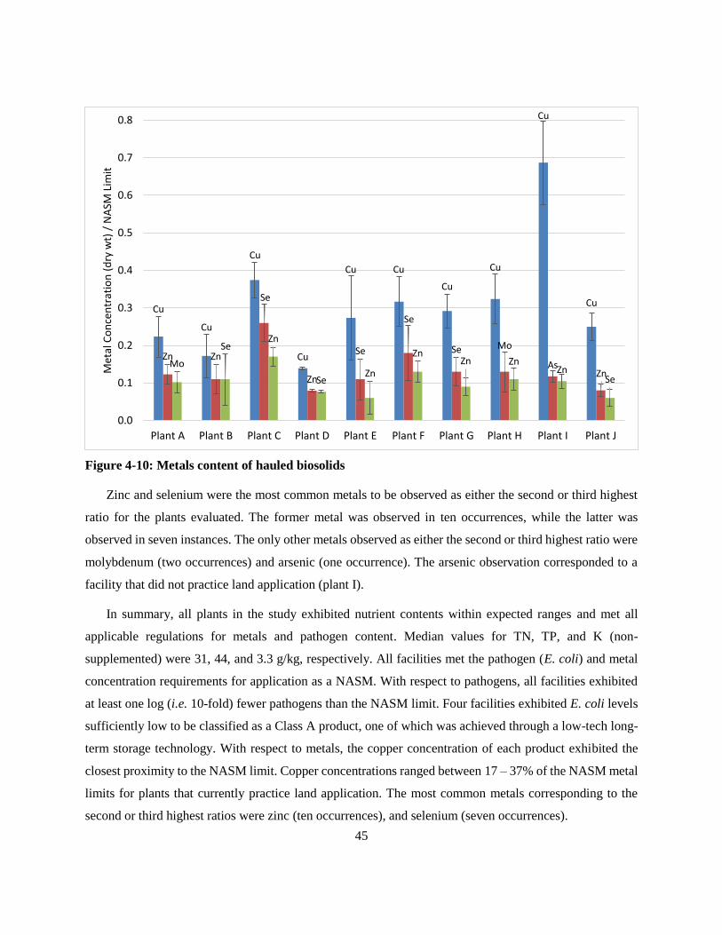
45

Figure 4-10: Metals content of hauled biosolids

Zinc and selenium were the most common metals to be observed as either the second or third highest

ratio for the plants evaluated. The former metal was observed in ten occurrences, while the latter was

observed in seven instances. The only other metals observed as either the second or third highest ratio were

molybdenum (two occurrences) and arsenic (one occurrence). The arsenic observation corresponded to a

facility that did not practice land application (plant I).

In summary, all plants in the study exhibited nutrient contents within expected ranges and met all

applicable regulations for metals and pathogen content. Median values for TN, TP, and K (non-

supplemented) were 31, 44, and 3.3 g/kg, respectively. All facilities met the pathogen (E. coli) and metal

concentration requirements for application as a NASM. With respect to pathogens, all facilities exhibited

at least one log (i.e. 10-fold) fewer pathogens than the NASM limit. Four facilities exhibited E. coli levels

sufficiently low to be classified as a Class A product, one of which was achieved through a low-tech long-

term storage technology. With respect to metals, the copper concentration of each product exhibited the

closest proximity to the NASM limit. Copper concentrations ranged between 17 – 37% of the NASM metal

limits for plants that currently practice land application. The most common metals corresponding to the

second or third highest ratios were zinc (ten occurrences), and selenium (seven occurrences).

Cu

Cu

Cu

Cu

Cu Cu

Cu

Cu

Cu

Cu

Zn Zn

Se

Zn

Se

Se

Se Mo

AsZn

Mo

SeZn

SeZn

ZnZn Zn

ZnSe

0.0

0.1

0.2

0.3

0.4

0.5

0.6

0.7

0.8

Plant A Plant B Plant C Plant D Plant E Plant F Plant G Plant H Plant I Plant J

Met

al C

on

cen

trat

ion

(d

ry w

t) /

NA

SM L

imit

46

4.5 GHG Emissions KPI Results

To facilitate a comparison of all the sludge handling operations on the basis of a common metric of

environmental sustainability, the inputs and outputs of each system were converted to normalized CO2

equivalents. The exercise determined the cumulative impact of each input and output on the carbon footprint

of the plant. Where possible, emission factors specific to Ontario (electricity, natural gas production) or

Canada (transportation fuel) were used to calculate the emissions associated with each input. In other cases,

literature values for chemical production (polymer, KOH) and chemical fertilizer production (N, P, K) were

utilized. The latter factors were used to determine the carbon off-sets gained by using biosolids as a fertilizer

through the avoidance of chemical fertilizer production for each nutrient.

The contributions of each system input and output to the net carbon footprint of each plant are shown

in Figure 4-11. Net GHG emissions ranged from -119 to 299 kg CO2 equivalents per dry tonne of raw

sludge produced. Of the eight plants that practiced land application disposition, six exhibited net negative

emissions, which ranged between -119 and -4 kg CO2 eq./dt. In each case, the carbon credits gained from

chemical fertilizer offsets exceeded the emissions associated with plant operations and biosolids trucking.

The outcome was due in large part to the reduction in carbon emissions associated with electricity

production in Ontario, which have dropped over 75% since 2010 (Environment and Climate Change

Canada, 2018). From a sustainability perspective, the outcome was noteworthy in two respects: a) land

application is the most common disposal method for small WWTPs in Ontario (Jin and Parker, 2017), and

b) all observations corresponded to facilities practicing conventional aerobic digestion, which is the most

common stabilization technology among small WWTPs in Ontario (Jin and Parker, 2017). The results

therefore indicate that when land application is practiced in combination with conventional treatment

processes, sludge handling practices in Ontario can be sustainable from a GHG perspective.

Of the plants studied, two facilities practiced land application but did not exhibit negative emissions. A

third facility (plant H) exhibited negative emissions (-4 kg CO2 eq./dt) to a substantially lesser degree than

other such plants within the sample [-119 to -86 kg CO2 eq./dt]. Plant B exhibited emissions near zero

(4 kg CO2 eq./dt), while the emissions associated with plant J (128 kg CO2 eq./dt) were substantially higher

than its peers that practiced land application. The net positive emissions observed for plant B were primarily

a result of the trucking emissions (137 kg CO2 eq./dt), which exceeded those associated with electricity

consumption (109 kg CO2 eq./dt). In the case of plant J, emissions associated with energy consumption and

chemical use exceeded the credits gained from fertilizer off-sets.

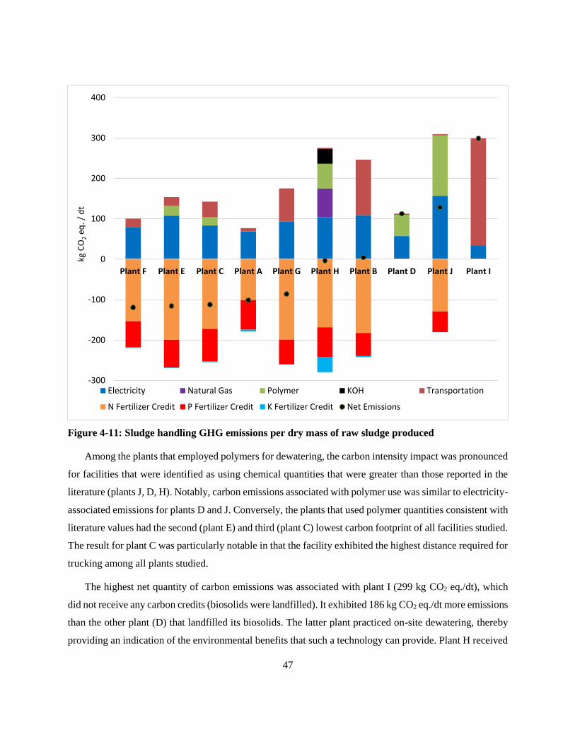
47

Figure 4-11: Sludge handling GHG emissions per dry mass of raw sludge produced

Among the plants that employed polymers for dewatering, the carbon intensity impact was pronounced

for facilities that were identified as using chemical quantities that were greater than those reported in the

literature (plants J, D, H). Notably, carbon emissions associated with polymer use was similar to electricity-

associated emissions for plants D and J. Conversely, the plants that used polymer quantities consistent with

literature values had the second (plant E) and third (plant C) lowest carbon footprint of all facilities studied.

The result for plant C was particularly notable in that the facility exhibited the highest distance required for

trucking among all plants studied.

The highest net quantity of carbon emissions was associated with plant I (299 kg CO2 eq./dt), which

did not receive any carbon credits (biosolids were landfilled). It exhibited 186 kg CO2 eq./dt more emissions

than the other plant (D) that landfilled its biosolids. The latter plant practiced on-site dewatering, thereby

providing an indication of the environmental benefits that such a technology can provide. Plant H received

-300

-200

-100

0

100

200

300

400

Plant F Plant E Plant C Plant A Plant G Plant H Plant B Plant D Plant J Plant I

kg C

O2

eq. /

dt

Electricity Natural Gas Polymer KOH Transportation

N Fertilizer Credit P Fertilizer Credit K Fertilizer Credit Net Emissions

48

a larger K fertilizer credit (-37 kg CO2 eq./dt) than its peers, which off-set the emissions associated with the

production of the KOH chemical used in the stabilization process (36 kg CO2 eq./dt). Its electricity-related

emissions totaled 104 kg CO2 eq./dt, of which 90 kg CO2 eq./dt were collectively associated with aerated

holding and odour control. Therefore, if the technology were to be implemented at facilities with no aerated

holding or odour control requirements (but with similar trucking distance), the technology would exhibit

emissions similar to the other observed sludge handling systems that were carbon sinks.

Figure 4-12 shows the carbon emissions associated with processes upstream of and including

stabilization for each plant in the study. The analysis provides insight into the emissions required for

mechanical treatment processes to achieve the observed product quality (pathogen content), irrespective of

downstream processes. As noted previously, plants D, J, and H generated a Class A product directly as a

result of their mechanical stabilization process (plant E generated it via passive long-term storage).

However, only the latter two facilities generated this quality of product using thermal processes that have

historically been accepted as being able to consistently generate a Class A product (Metcalf & Eddy, 2013).

Plant D employed conventional aerobic digestion, which would be expected to reduce pathogen levels to

Class B requirements (Metcalf & Eddy, 2013). From Figure 4-12, it can be seen that the highest emissions

were associated with plants H and J, which highlighted the environmental cost (GHG impact) of obtaining

a Class A product through thermal-mechanical processes.

In the case of plant J, both the thickening and stabilization steps were necessary to generate the Class A

product. Emissions associated with pumping, thickening, and stabilization electricity consumption

(152 kg CO2 eq./dt) and thickening polymer usage (31 kg CO2 eq. / dt) summed to 183 kg CO2 eq./dt. For

plant H, electricity associated with pumping, stabilization, and upstream dewatering (14 kg CO2 eq./dt),

natural gas (71 kg CO2 eq./dt), polymer usage (62 kg CO2 eq./dt), and KOH (36 kg CO2 eq./dt) were

necessary to generate the final product. The addition of KOH generated a carbon credit of -35 kg CO2 eq./dt

(credits for N and P fertilizer avoidance were not a result of the treatment process selection). Subtracting

the credits associated with the K fertilizer avoidance, the emissions associated with the inputs identified

totaled 148 kg CO2 eq./dt. Examining exclusively stabilization and related emissions, both plants J and H

exhibited emissions substantially higher than the plants that generated a Class B/NASM quality product.

The emissions associated with Class B generation ranged between 26 – 109 kg CO2 eq./dt.

49

Figure 4-12: GHG emissions associated with processes upstream of and including stabilization

In summary, GHG emissions associated with sludge handling operations ranged from -119 to 299

kg CO2 eq./dt among all plants studied. Six facilities exhibited net-negative emissions, which ranged

between -119 to -4 kg CO2 eq./dt. The five systems that yielded the lowest emissions employed process

configurations that were relatively common province-wide, which suggests that other sludge handling

systems across the province may be carbon sinks as well. Among the two plants (H and J) that practiced

thermal stabilization processes (thermo-alkali hydrolysis and ATAD) for the purposes of generating a

Class A product (E. coli content), total emissions associated with stabilization and auxiliary processes were

148 and 183 kg CO2 eq./dt, respectively. Both values were higher than plants that generated Class B/NASM

quality products, which ranged between 26 and 109 kg CO2 eq./dt. The discrepancy highlighted the

environmental trade-offs associated with Class A product generation through such stabilization methods.

-50

0

50

100

150

200

Plant F Plant I Plant D Plant A Plant C Plant G Plant E Plant B Plant H Plant J

kg C

O2

eq. /

dt

Electricity Natural Gas Polymer KOH K Fertilizer Credit Net Emissions

50

4.6 Impact of Innovative Technology on Sustainability

Part of the rationale for evaluating WWTPs that employed innovative thickening, stabilization, and

dewatering technologies was to quantify the impact on sustainability of implementing such technologies

within other plants that currently employ conventional process configurations. From an economic

sustainability standpoint, the operational inputs and outputs detailed in sections 4.1 – 4.5 could be used as

benchmarks to determine the localized costs associated with operating each technology. However, to assess

the environmental sustainability (through GHG impact analysis) of implementing such technologies in

facilities with site-specific conditions (e.g. storage practices, trucking distance), further desktop analysis

was conducted.

To perform the evaluation, all the innovative technologies within the plants studied (rotary disc

thickening, thermo-alkali hydrolysis, ATAD, GeoTube™, rotary press, centrifuge) were considered for

incorporation into the conventional plants (A, B, F, G, I) based on the input/outputs observed from the

plants that employed the technologies (C, D, E, H, J). Upon initial screening, the thermo-alkali hydrolysis

and ATAD technologies were removed from consideration due to the substantial GHG emissions observed

in the study (H and J, respectively). For the remaining technologies, the KPIs were re-calculated using site-

specific conditions, and the resulting GHG emissions were compared to the base case for each plant. Further

scenarios involving low and high polymer usage were evaluated separately due to the discrepancy between

the low and high observed usage for each technology (rotary press and centrifuge).

The change in plant GHG emissions after innovative technology implementation (relative to the base

case) are shown in Figure 4-13. Two plants (B, I) exhibited a reduction in GHG emissions under all

scenarios, one plant (A) exhibited an increase in emissions under all scenarios, and two facilities (F, G)

exhibited increases and decreases depending on the technology/configuration selected. In each case, the

base case trucking requirements were the primary factor regarding whether a new technology would

increase or decrease emissions.

Among the five plants evaluated for new technology implementation, Plants B and I had the highest

base case trucking requirements and did not employ on-site storage. Therefore, both plants exhibited the

greatest reduction in transportation fuel consumption when scenarios involving thickening or dewatering

implementation were implemented. In both cases, the fuel-related savings off-set the emissions associated

with polymer production under all scenarios.

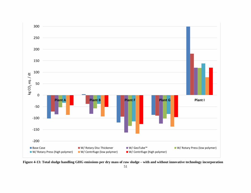
51

Figure 4-13: Total sludge handling GHG emissions per dry mass of raw sludge – with and without innovative technology incorporation

-200

-150

-100

-50

0

50

100

150

200

250

300

Plant A Plant B Plant F Plant G Plant I

kg C

O2

eq. /

dt

Base Case W/ Rotary Disc Thickener W/ GeoTube™ W/ Rotary Press (low polymer)

W/ Rotary Press (high polymer) W/ Centrifuge (low polymer) W/ Centrifuge (high polymer)

52

Plant I also benefited from two unique outcomes of dewatering technology implementation that resulted

in additional GHG savings relative to its peers. The first outcome involved the change in the trucking route

that was made possible under the new technology scenario relative to the base case. Under any scenario

where cake was generated at the plant (centrifuge and rotary press), the biosolids product could be

transported directly to the landfill. The need for transport to both the drying bed and landfill would be

eliminated, thereby reducing net fuel requirements. For the plants that land applied their biosolids, the

trucking route was assumed to be the same under the new technology scenarios since the facilities would

not be able to land apply biosolids at new times under any new scenario.

The second outcome involved the volume and fuel economies of the trucks employed by the facilities.

In the base case, Plant I employed a truck with a volume lower than that of the conventional trucks in place

at other facilities (16.5 versus 40 m3), but did not receive proportionally lower fuel economy (2.0 versus

1.72 L/km). Under scenarios where cakes were generated, Plant I could instead use a truck similar to that

employed by its peer northern facility (plant D), which consumed 5.0 L/km and hauled 8.5 m3 per trip. At

all other plants, the truck selection would remain the same under the new scenarios since the different truck

would not generate additional fuel (and related-GHG emission) savings.

Plant A was the only facility that did not exhibit emissions reduction under any innovative technology

scenario. The outcome was primarily due to the short trucking distance required, which resulted in

substantially less fuel savings than plants with higher trucking requirements (B, G, I). Under all new

scenarios, the fuel-related emission savings did not off-set the added emissions associated with polymer

usage for plant A.

Plant F exhibited similar base case trucking distance requirements to plant A (8 vs 3 km, respectively),

but unlike its peer, there were some scenarios in which dewatering implementation would reduce plant F

emissions. The difference was due to the changes in existing technologies that would be possible under the

new scenarios. Unlike plant A, plant F employs electricity for aerated holding/storage that would be

eliminated under all dewatering scenarios. Specifically, the cake products generated by mechanical

dewatering processes do not require aeration in storage, and a GeoTube™ functions as both a dewatering

and storage device. Under select new dewatering scenarios in plant F, the combination of electricity- and

fuel- related emission savings resulted in a net GHG savings relative to the base case. Of note, the

implementation of a thickening technology at plant F would not negate the need for aerated holding. In this

case, a liquid product would still be formed and require aeration for the same reasons as for the existing

process: to maintain solids suspension and facilitate easier pumping of the material during haulage events.

53

As such, the electricity-related emissions associated with holding were included in the thickening scenario,

and the net impact was higher plant emissions under this scenario.

Two facilities (F, G) had scenarios where GHG emissions would either be reduced or increased

depending on the technology and configuration selected. With rotary thickening implementation, Plant F

exhibited an increase in carbon emissions, while plant G exhibited a minor decrease in emissions

(- 3 kg CO2 eq./dt). At both plants, the implementation of GeoTube™ or centrifuge technology resulted in

GHG reductions in all scenarios. The net outcome (increased or decreased plant emissions) of implementing

rotary press dewatering was dependent on the assumed polymer dosage. A high polymer dose resulted in

higher plant emissions for both facilities, while a low polymer dose resulted in lower plant emissions. As a

result, polymer usage was identified as an important parameter when considering whether to implement a

new technology for the purpose of improving the environmental sustainability.

In summary, this desktop innovative technology analysis revealed cases where GHG emissions were

reduced under all technology implementation scenarios (plants B and I), increased under all scenarios

(plant A), and dependent on the configuration selected (plants F and G). For each scenario, the net outcome

was primarily dependent on whether the GHG emissions saved from fuel consumption reduction off-set the

emissions associated with thickening/dewatering polymer production. Plants B and I exhibited the highest

base case trucking requirements, subsequently received the greatest reduction in trucking fuel consumption

emissions, and reduced net carbon emissions under all scenarios. Conversely, the finding for plant A

suggests that thickening or dewatering technology implementation at facilities with low initial trucking

requirements may increase the plant’s carbon impact if fuel-related GHG savings do not off-set the

additional emissions associated with polymer usage. A possible exception (plant F) was noted for cases

where the dewatering technology can replace an existing unit process (e.g. aerated holding tanks) and thus

eliminate the emissions associated with the existing operation.

54

Chapter 5

Conclusions and Recommendations

5.1 Conclusions

A benchmarking exercise was completed to characterize the sustainability of sludge handling in small

WWTPS in Ontario and a desktop analysis was conducted to determine the GHG impact of incorporating

innovative technologies into conventional sludge handling configurations. The benchmarking component

involved evaluating ten plants across the province on a variety of sustainability metrics: energy

consumption, chemical use, biosolids disposition, biosolids quality, and GHG emissions. The desktop

assessment involved applying select innovative technologies within the study sample to those that employed

conventional processes, and calculating the resulting GHG impact.

Among all plants studied, overall electricity consumption for sludge handling ranged from 0.9 – 3.9

kWh/dry kg (median = 2.2 kWh/dry kg). The maximum consumption corresponded to the facility practicing

ATAD stabilization, while the highest value among conventional aerobic digestion plants was

2.7 kWh/dry kg. Consumption for stabilization processes was found to range from 0.3 – 3.8 kWh/dry kg

(median = 1.6 kWh/dry kg). The maximum value corresponded to the ATAD process, while the minimum

consumption corresponded to the thermo-alkali hydrolysis process. The low value for the latter process

indicated that such a technology may be a viable option for reducing electricity consumption in facilities

where aerated holding and odour control are not necessary.

Among the eight plants that practiced conventional aerobic digestion, consumption normalized by

quantity of VSS destruction was found to range from 4.9 – 56 kWh/dry kg VSS (median = 8.7 kWh/dry kg

VSS). The ATAD facility exhibited the highest consumption among all plants (63 kWh/dry kg VSS). Of

the eight plants that practiced conventional aerobic digestion, the range of the five lowest values (5 – 9

kWh/dry kg VSS) was substantially lower than the range of the three highest values (15 – 56 kWh/dry kg

VSS).

Electricity consumption for mechanical dewatering processes ranged from 0.06 – 0.10 kWh/dry kg,

which represented 2 – 5% of total sludge handling power draw for such plants. Chemical usage for

dewatering processes ranged between 8 – 24 kg polymer/dt (centrifuges) and 20 – 28 kg polymer/dt (rotary

presses), while the GeoTube™ process used 9 kg polymer/dt. The three highest observed chemical usage

values were greater than those found in literature, which suggested that the polymers were either over-dosed

to some extent and/or were not as effective coagulating/flocculating agents as those employed in literature

55

case studies. The solids content of the product generated ranged between 16.9 – 22.5% (centrifuges) and

17.2 – 18.4% (rotary presses). The GeoTube™ process generated a 9.2% solids product.

The weighted average round-trip distance for disposition between the WWTP and the final destination

ranged between 8 – 83 km and the normalized transportation fuel consumption ranged between 1 – 99 L/dt.

The difference between trucking distance and transportation fuel consumption was largest when comparing

facilities that employed chemically enhanced dewatering against those that did not. The plant with the

maximum trucking distance (83 km) practiced mechanical dewatering and consumed between 72 – 85%

less fuel than the plants with the second and third highest trucking distances (both of which did not practice

dewatering).

All the sampled plants exhibited nutrient contents within expected ranges and contaminant

(metals/pathogens) contents below regulated levels for application as a NASM. All facilities exhibited at

least one log (i.e. 10-fold) fewer pathogens than the NASM limit. Four facilities generated product that met

Class A requirements for E. coli content, one of which was achieved through a low-tech long-term storage

technology (GeoTube™). The copper concentration of each product exhibited the closest proximity to the

NASM limit. It ranged between 17 – 37% among plants that currently practiced land application. The most

common metals corresponding to the second or third highest ratios were zinc and selenium.

Carbon emissions ranged from -119 to 299 kg CO2 eq./dt among all plants studied. Six of the eight

facilities that practiced land application exhibited net-negative emissions, ranging from -119 to -4 kg CO2

eq./dt. Land application is the most common biosolids disposal method across Ontario, which indicates that

sludge handling practices of several plants province-wide are sustainable from a GHG standpoint. Among

the two plants that practiced an alternative stabilization processes (thermo-alkali hydrolysis and ATAD) for

the purpose of generating a product that meets Class A requirements for E. coli content, emissions

associated with stabilization and auxiliary processes were 148 and 183 kg CO2 eq./dt, respectively. Both

quantities were substantially higher than those associated with processes that generated Class B/NASM

quality products (26 – 109 kg CO2 eq./dt) and highlighted the environmental trade-offs associated with

achieving Class A pathogen levels through such stabilization methods.

The innovative technology assessment suggests that existing trucking requirements and polymer dosage

are the primary factors that determine whether or not the technologies evaluated would improve

environmental sustainability if implemented. The assessment revealed one facility where GHG emissions

would be increased under all new technology scenarios, two facilities where emissions would be decreased

56

under all scenarios, and two facilities where GHG emissions would either be increased or decreased

depending on the technology and polymer dosage selected.

From an operations and sustainability standpoint, the benchmarking approach developed can be

employed by plant owners and operators who seek to better understand how their utility is performing

relative to peers of similar capacity and scope of operations, identify areas of need and further investigation,

and move toward improving the long-term sustainability of their operations. The substantially different

levels of normalized inputs/outputs observed demonstrate the value of benchmarking: it provides owners

and operators with a means to compare, evaluate, and potentially find opportunities for optimization within

their own systems, and provides a base case from which to compare future technology implementation.

5.2 Recommendations

Regardless of the industry it is being applied in, the practice of benchmarking provides more insight if

more specimens are included in the sample. Therefore, it is first recommended that sludge handling systems

in additional small WWTPs be evaluated using the KPI framework and audit methodology developed in

the present study. Different plants may potentially perform better than the ten facilities investigated in the

current study, which would potentially provide insight into better sludge handling management practices

for implementation elsewhere. Conversely, plants may be identified as lagging behind the current group in

terms of sustainability performance. If changes were made to improve performance in such plants, the

collective sustainability of sludge handling province-wide would increase as well. Facilities from other

parts of Canada could also be evaluated to determine how facilities in differing provinces rank amongst

each other, determine whether particular regional practices are more sustainable than others, and promote

knowledge transfer between participating municipalities to move toward the goal of universally

implementing best practices for sludge management.

Within the category of small WWTPs, it is recommended that the audit process be extended to

include liquid stream operations. The inputs to the liquid train process at many of the facilities are similar

to those for sludge handling: electricity to operate blowers and pumps, and chemicals to remove precipitate

soluble phosphorus. Energy, chemical, GHG, and effluent quality-related metrics could be evaluated on a

number of bases, depending on applicability: volume of flow treated, mass of pollutant load to the plant,

and/or mass of pollutant removed from the wastewater. Such analyses would provide additional insight into

the sustainability of the entire treatment facility.

57

Finally, it is recommended that the audit procedure be extended to include larger facilities. The

current study focused on small WWTPs because of the unique challenges that such plants often encounter,

but facilities of all sizes typically employ similar inputs and outputs that have associated economic and

environmental impacts. As such, improving the performance of all plants would be beneficial to the long-

term economic and environmental sustainability of the wastewater treatment industry.

58

References

AECOM (2012). Leveraging the energy of the group to manage the energy of the utility: the NWWBI

adopts industry tools to improve energy performance. Proceedings of the Water Environment Federation,

2012. (20), 2383-2402

AECOM (2018). National water and wastewater benchmarking initiative. Public report. Accessed online:

http://nationalbenchmarking.ca/public/docs/Public%20Report%20_2016_compiled.pdf

AMBI (2017). Alberta municipal benchmarking initiative – wastewater. Accessed online:

https://banff.ca/DocumentCenter/View/4695

Alanya, S., Dewulf, J., & Duran, M. (2015). Comparison of overall resource consumption of biosolids

management system processes using exergetic life cycle assessment. Environmental Science &

Technology, 49(16), 9996-10006.

Alvarez-Gaitan, J. P., Short, M. D., Lundie, S., & Stuetz, R. (2016). Towards a comprehensive

greenhouse gas emissions inventory for biosolids. Water Research, 96, 299-307.

Bailey, E. L., Whitfield, T., Revels, J., & D’Adamo, P. (2014). Benchmarking of biosolids and residuals

handling operations: building the measuring stick. Proceedings of the Water Environment Federation,

2014 (6), 2773-2797.

Balmér, P. (2000). Operation costs and consumption of resources at Nordic nutrient removal plants.

Water Science and Technology, 41(9), 273-279.

Balmér, P., & Hellström, D. (2012). Performance indicators for wastewater treatment plants. Water

Science and Technology, 65(7), 1304-1310.

Barber, W. P. (2009). Influence of anaerobic digestion on the carbon footprint of various sewage sludge

treatment options. Water and Environment Journal, 23(3), 170-179.

Beavis, P., & Lundie, S. (2003). Integrated environmental assessment of tertiary and residuals treatment-

LCA in the wastewater industry. Water Science and Technology, 47(7-8), 109-116.

Belloir, C., Stanford, C., & Soares, A. (2015). Energy benchmarking in wastewater treatment plants: the

importance of site operation and layout. Environmental Technology, 36(2), 260-269.

Benedetti, L., Dirckx, G., Bixio, D., Thoeye, C., & Vanrolleghem, P. A. (2008). Environmental and

economic performance assessment of the integrated urban wastewater system. Journal of Environmental

Management, 88(4), 1262-1272.

Biograce. (2011). Harmonised calculations of biofuel greenhouse gas emissions in Europe – list of

additional standard values. Version 1. Accessed online:

http://www.biograce.net/img/files/BioGrace_additional_standard_values_-_version_1_-_Public.pdf

Bodik, I., & Kubaska, M. (2013). Energy and sustainability of operation of a wastewater treatment

plant. Environment Protection Engineering, 39(2), 15-24.

http://nationalbenchmarking.ca/public/docs/Public%20Report%20_2016_compiled.pdf

https://banff.ca/DocumentCenter/View/4695

http://www.biograce.net/img/files/BioGrace_additional_standard_values_-_version_1_-_Public.pdf

59

Bridle, T., & Skrypski-Mantele, S. (2000). Assessment of sludge reuse options: a life-cycle

approach. Water Science and Technology, 41(8), 131-135.

Carlson, S.W., Walburger, A., & AWWA Research Foundation (2007). Energy index development for

benchmarking water and wastewater utilities. AWWA Research Foundation, Denver, CO

Chai, C., Zhang, D., Yu, Y., Feng, Y., & Wong, M. S. (2015). Carbon footprint analyses of mainstream

wastewater treatment technologies under different sludge treatment scenarios in China. Water, 7(3), 918-

938.

De Haas, D. W., Foley, J., Marshall, B., Dancey, M., Vierboom, S., & Bartle-Smith, J. (2015).

Benchmarking wastewater treatment plant energy use in Australia. Proceedings of the Ozwater, 15.

Emmerson, R. H. C., Morse, G. K., Lester, J. N., & Edge, D. R. (1995). The life‐cycle analysis of small‐

scale sewage‐treatment processes. Water and Environment Journal, 9(3), 317-325.

ENERGY STAR (2014). Score for wastewater treatment plants in the United States. ENERGY STAR

Portfolio Manager. Accessed online: https://www.energystar.gov/sites/default/files/tools/Wastewater.pdf

Environment and Climate Change Canada. (2018). National inventory report 1990 – 2016: Greenhouse

gas sources and sinks in Canada. Accessed online: https://unfccc.int/documents/65715

Eyre, K., Keyzers, T., Becker J. G., Seagren E. A., & Meingast, C. (2018). Pilot scale evaluation of a two-

stage, low-cost low-tech class A biosolids treatment. Proceedings of the WEF Residuals and Biosolids

Conference, 2018.

Foladori, P., Vaccari, M., & Vitali, F. (2015). Energy audit in small wastewater treatment plants:

methodology, energy consumption indicators, and lessons learned. Water Science and Technology, 72(6),

1007-1015.

Fertilizers Act (R.S.C., 1985, c. F-10). Accessed online: http://laws-lois.justice.gc.ca/eng/acts/F-10/

Fertilizers Regulations (C.R.C., c. 666). Accessed online: http://laws-

lois.justice.gc.ca/eng/regulations/C.R.C.,_c._666/page-2.html#h-7

Gallego, A., Hospido, A., Moreira, M. T., & Feijoo, G. (2008). Environmental performance of wastewater

treatment plants for small populations. Resources, Conservation and Recycling, 52(6), 931-940.

Gu, Y., Dong, Y. N., Wang, H., Keller, A., Xu, J., Chiramba, T., & Li, F. (2016). Quantification of the

water, energy and carbon footprints of wastewater treatment plants in China considering a water–energy

nexus perspective. Ecological Indicators, 60, 402-409.

Hanna, S., Dvorak, B., Dahab, M., & Thompson, M. (2017). Benchmarking the Electric Intensity of

Small Nebraska Wastewater Treatment Facilities. Proceedings of the Water Environment

Federation, 2017(6), 4930-4947.

Hara, K., & Mino, T. (2008). Environmental assessment of sewage sludge recycling options and treatment

processes in Tokyo. Waste Management, 28(12), 2645-2652.

https://www.energystar.gov/sites/default/files/tools/Wastewater.pdf

https://unfccc.int/documents/65715

http://laws-lois.justice.gc.ca/eng/acts/F-10/

http://laws-lois.justice.gc.ca/eng/regulations/C.R.C.,_c._666/page-2.html#h-7

http://laws-lois.justice.gc.ca/eng/regulations/C.R.C.,_c._666/page-2.html#h-7

60

Haslinger, J., Lindtner, S., & Krampe, J. (2016). Operating costs and energy demand of wastewater

treatment plants in Austria: benchmarking results of the last 10 years. Water Science and Technology,

wst2016390.

Hong, J., Hong, J., Otaki, M., & Jolliet, O. (2009). Environmental and economic life cycle assessment for

sewage sludge treatment processes in Japan. Waste Management, 29(2), 696-703.

Hospido, A., Moreira, T., Martín, M., Rigola, M., & Feijoo, G. (2005). Environmental evaluation of

different treatment processes for sludge from urban wastewater treatments: Anaerobic digestion versus

thermal processes (10 pp). The International Journal of Life Cycle Assessment, 10(5), 336-345.

Houillon, G., & Jolliet, O. (2005). Life cycle assessment of processes for the treatment of wastewater

urban sludge: energy and global warming analysis. Journal of Cleaner Production, 13(3), 287-299.

IPCC (2006). Guidelines for national greenhouse gas inventories. Chapter 3: Chemical Industry

Emissions.

ISO 14040 (2006). Environmental management: life cycle assessment – principles and framework.

Geneva, Switzerland.

ISO 14044 (2006). Environmental management: life cycle assessment – requirements and guidelines.

Geneva, Switzerland.

Jin, C. & Parker, W. (2017). Needs assessment for biosolids processing in Ontario. Accessed online:

https://sowc.ca/wp-content/uploads/2017/10/SOWC-report_-Needs-Assessment-for-Sludge-Processing-

Technologies-in-Onta....pdf

Johansson, K., Perzon, M., Fröling, M., Mossakowska, A., & Svanström, M. (2008). Sewage sludge

handling with phosphorus utilization–life cycle assessment of four alternatives. Journal of Cleaner

Production, 16(1), 135-151.

Krampe, J. (2013). Energy benchmarking of South Australian WWTPs. Water Science and

Technology, 67(9), 2059-2066.

Kongshaug, G. (1998). Energy consumption and greenhouse gas emissions in fertilizer production. In IFA

Tech. Conf., Marrakech, Morocco, 1998. Int. Fertilizer Industry Association.

Li, X., Takaoka, M., Zhu, F., Wang, J., Oshita, K., & Mizuno, T. (2013). Environmental and economic

assessment of municipal sewage sludge management–a case study in Beijing, China. Water Science and

Technology, 67(7), 1465-1473.

Lindtner, S., Kroiss, H., & Nowak, O. (2004). Benchmarking of municipal waste water treatment plants

(an Austrian project). Water Science and Technology, 50(7), 265-271.

Lindtner, S., Schaar, H., & Kroiss, H. (2008). Benchmarking of large municipal wastewater treatment

plants treating over 100,000 PE in Austria. Water Science and Technology, 57(10), 1487-1493.

https://sowc.ca/wp-content/uploads/2017/10/SOWC-report_-Needs-Assessment-for-Sludge-Processing-Technologies-in-Onta....pdf

https://sowc.ca/wp-content/uploads/2017/10/SOWC-report_-Needs-Assessment-for-Sludge-Processing-Technologies-in-Onta....pdf

61

Liu, B., Wei, Q., Zhang, B., & Bi, J. (2013). Life cycle GHG emissions of sewage sludge treatment and

disposal options in Tai Lake Watershed, China. Science of the Total Environment, 447, 361-369.

Lorenzo-Toja, Y., Vázquez-Rowe, I., Amores, M. J., Termes-Rifé, M., Marín-Navarro, D., Moreira, M.

T., & Feijoo, G. (2016). Benchmarking wastewater treatment plants under an eco-efficiency

perspective. Science of the Total Environment, 566, 468-479.

Lundin, M., Olofsson, M., Pettersson, G. J., & Zetterlund, H. (2004). Environmental and economic

assessment of sewage sludge handling options. Resources, Conservation and Recycling, 41(4), 255-278.

Mamais, D., Noutsopoulos, C., Dimopoulou, A., Stasinakis, A., & Lekkas, T. D. (2015). Wastewater

treatment process impact on energy savings and greenhouse gas emissions. Water Science and

Technology, 71(2), 303-308.

Metcalf & Eddy (2013). Wastewater engineering: Treatment and reuse (4th ed.). Boston: McGraw-Hill

Mizuta, K., & Shimada, M. (2010). Benchmarking energy consumption in municipal wastewater

treatment plants in Japan. Water Science and Technology, 62(10), 2256-2262.

Ontario Ministry of Environment and Climate Change – MOECC January 2008. Design Guidelines for

Sewage Works. PIBS 6879. Accessed online: https://www.ontario.ca/document/design-guidelines-

sewage-works-0

Murray, A., Horvath, A., & Nelson, K. L. (2008). Hybrid life-cycle environmental and cost inventory of

sewage sludge treatment and end-use scenarios: a case study from China.

Niu, D. J., Huang, H., Dai, X. H., & Zhao, Y. C. (2013). Greenhouse gases emissions accounting for

typical sewage sludge digestion with energy utilization and residue land application in China. Waste

Management, 33(1), 123-128.

Nowak, O. (2003). Benchmarks for the energy demand of nutrient removal plants. Water Science and

Technology, 47(12), 125-132.

New York State Energy and Research Development Authority (NYSERDA) (1998). On-line process

monitoring and electric submetering at six municipal wastewater treatment plants. Accessed online:

https://www.nyserda.ny.gov/About/Publications/Research-and-Development-Technical-Reports/Water-

and-Wastewater-Technical-Reports

New York State Energy and Research Development Authority (NYSERDA) (2006). Municipal

wastewater treatment plant energy evaluation. Accessed online:



New York State Energy and Research Development Authority (NYSERDA) (2008). Statewide

assessment of energy use by the municipal water and wastewater sector. Accessed online:



https://www.ontario.ca/document/design-guidelines-sewage-works-0

https://www.ontario.ca/document/design-guidelines-sewage-works-0

https://www.nyserda.ny.gov/About/Publications/Research-and-Development-Technical-Reports/Water-and-Wastewater-Technical-Reports






62

O. Reg. 267/03: GENERAL under Nutrient Management Act, 2002, S.O. 2002, c. 4. Accessed online:

https://www.ontario.ca/laws/regulation/030267

Patziger, M. (2017). Efficiency and Development Strategies of Medium–Sized Wastewater Treatment

Plants in Central and Eastern Europe: Results of a Long-Term Investigation Program in Hungary. Journal

of Environmental Engineering, 143(6), 04017008.

Peters, G. M., & Lundie, S. (2001). Life‐Cycle Assessment of Biosolids Processing Options. Journal of

Industrial Ecology, 5(2), 103-121.

Poulsen, T. G., & Hansen, J. A. (2003). Strategic environmental assessment of alternative sewage sludge

management scenarios. Waste Management & Research, 21(1), 19-28.

Recycled Organics Unit. (2006). Life cycle inventory and life cycle assessment for windrow composting

systems. The Univ. of New South Wales, Sydney, Australia.

Remy, C., Lesjean, B., & Waschnewski, J. (2012). Identifying energy and carbon footprint optimization

potentials of a sludge treatment line with life cycle assessment. Water Science and Technology, 67(1), 63-

73.

Rodriguez-Garcia, G., Molinos-Senante, M., Hospido, A., Hernández-Sancho, F., Moreira, M. T., &

Feijoo, G. (2011). Environmental and economic profile of six typologies of wastewater treatment

plants. Water Research, 45(18), 5997-6010.

Science Applications International Corporation (SAIC) (2006). Water & wastewater industry energy best

practice guidebook. Accessed online: http://www.oracwa.org/pdf/wi-waterandwastewater-guidebook.pdf

Silva, C., Ramalho, P., Quadros, S., Alegre, H., & Rosa, M. J. (2012). Results of ‘PASt21’–the

Portuguese initiative for performance assessment of water and wastewater treatment plants. Water

Science and Technology: Water Supply, 12(3), 372-386.

Silva, C., & Rosa, M. J. (2015). Energy performance indicators of wastewater treatment: a field study

with 17 Portuguese plants. Water Science and Technology, 72(4), 510-519.

Silva, C., Matos, J. S., & Rosa, M. J. (2016). Performance indicators and indices of sludge management

in urban wastewater treatment plants. Journal of Environmental Management, 184, 307-317.

Singh, P., Kansal, A., & Carliell-Marquet, C. (2016). Energy and carbon footprints of sewage treatment

methods. Journal of Environmental Management, 165, 22-30.

Stefaniak, J., Żelazna, A., & Pawłowski, A. (2014). Environmental assessment of different dewatering

and drying methods on the basis of life cycle assessment. Water Science and Technology, 69(4), 783-788.

Suh, Y. J., & Rousseaux, P. (2002). An LCA of alternative wastewater sludge treatment

scenarios. Resources, Conservation and Recycling, 35(3), 191-200.

https://www.ontario.ca/laws/regulation/030267

http://www.oracwa.org/pdf/wi-waterandwastewater-guidebook.pdf

63

Svanström, M., Fröling, M., Olofsson, M., & Lundin, M. (2005). Environmental assessment of

supercritical water oxidation and other sewage sludge handling options. Waste Management &

Research, 23(4), 356-366.

Tao, X., & Chengwen, W. (2012, May). Energy consumption in wastewater treatment plants in China.

In World Congress on Water, Climate and Energy (pp. 1-6).

T-4-93 - Safety Guidelines for Fertilizers and Supplements Accessed online:

http://www.inspection.gc.ca/plants/fertilizers/trade-memoranda/t-4-

93/eng/1305611387327/1305611547479

US EPA 1993, Standards for the Use or Disposal of Sewage Sludge, US Code of Federal Regulations,

Part 503, Office of the Federal Register National archives and Records Administration, Washington, DC

Vera, I., Sáez, K., & Vidal, G. (2013). Performance of 14 full-scale sewage treatment plants: Comparison

between four aerobic technologies regarding effluent quality, sludge production and energy consumption.

Environmental Technology, 34(15), 2267-2275.

Wang, H., Yang, Y., Keller, A. A., Li, X., Feng, S., Dong, Y. N., & Li, F. (2016). Comparative analysis

of energy intensity and carbon emissions in wastewater treatment in USA, Germany, China and South

Africa. Applied Energy, 184, 873-881.

WERF (2016). Current Energy Position of New York State Wastewater Treatment Facilities. Water

Environment Research Foundation.

Xu, C., Chen, W., & Hong, J. (2014). Life-cycle environmental and economic assessment of sewage

sludge treatment in China. Journal of Cleaner Production, 67, 79-87.

Yang, L., Zeng, S., Chen, J., He, M., & Yang, W. (2010). Operational energy performance assessment

system of municipal wastewater treatment plants. Water Science and Technology, 62(6), 1361-1370.

http://www.inspection.gc.ca/plants/fertilizers/trade-memoranda/t-4-93/eng/1305611387327/1305611547479

http://www.inspection.gc.ca/plants/fertilizers/trade-memoranda/t-4-93/eng/1305611387327/1305611547479

64

Appendix A

Plant A Summary

Overview

Plant A is an extended aeration WWTP located in Southern Ontario and operated by OCWA. Sludge is

stabilized via aerobic digestion and the biosolids are stored in an on-site lagoon. During spreading season,

the biosolids are hauled and applied to land for agricultural purposes.

BioWin Modelling

A BioWin™ model based on observed operational data was generated to estimate raw sludge

production and VSS destruction, and to screen for problematic plant data. A summary of key model outputs

and the corresponding mean observed value (where applicable) is shown in Table A1. The two observed

MLSS values correspond to each train of liquid treatment. The model process flow sheet is shown in Figure

A1. The model outputs were generally consistent with reported values.

Table A1: Plant A BioWin Model Results

Parameter Units Predicted Value Observed Value

(2014-2016)

MLSS mg/L 2263 2327, 2410

Dry mass of sludge wasted per day kg TSS/d 405 408

Dry mass of solids returned per day (digester

decant)

kg TSS/d 88 --

Dry mass of solids returned per day (lagoon

decant)

kg TSS/d 66 --

Net dry mass of sludge generated per day kg TSS/d 251 --

Dry mass of VSS input to digester per day kg VSS/d 247 --

Dry mass of VSS output by digester per day kg VSS/d 199 --

Dry mass of VSS destroyed per day kg VSS/d 48 --

Volume of biosolids generated per day m3 7.0 7.0

TSS content of hauled biosolids % 2.8 4.9

VSS content of hauled biosolids % 56 54.5

65

Figure A1: Plant A BioWin Model PFD

Uncertainty

To estimate uncertainty in raw sludge production, the standard deviation in reported sludge production

(59 dry kg/d) was divided by the reported mean sludge production (408 dry kg/d) and converted to a

percentage. Raw data was provided in the form of a daily average for each month within a two year period

(2015-2016), hence the sample size was n = 24. Using this measure, the uncertainty was determined to be

15%.

Energy

On-site power draw measurements were taken on all pieces of equipment related to sludge handling

and multiplied by the daily motor run-time (obtained from plant records) to determine the daily kWh

consumption for each motor of interest (Table A2). The total draw for each category of equipment

(stabilization, pumping) was calculated and divided by mass of raw sludge generated daily (Table A3).

Digester electricity consumption was also divided by the daily quantity of VSS destruction (Table A3).

66

Table A2: Plant A Energy Measurements

Category/Motor Voltage

(V)

Current

(A)

Power

Factor

(PF)

Power

Draw (kW)

Motor Run-

Time (Hr/d)

Daily Electricity

Consumption (kWh/d)

Stabilization

Digester Blower 607 11.4 0.965 14.7 24 353

Sub-total 353

Pumping

WAS pump 1 607 4.4 0.856 3.5 11.8 41

WAS pump 2 606 3.6 0.856 2.8 12.2 34

Sub-total 75

Total 428

Table A3: Plant A Energy KPI Results (Electricity Consumption)

Category Normalized Electricity Consumption (kWh/dry kg)

Stabilization 1.41

Pumping 0.30

Total 1.71

Digester Efficiency 7.4 (kWh / dry kg VSS destroyed)

Chemical Usage

Plant A does not employ the use of chemicals for its sludge handling process.

Biosolids Disposition

Average round-trip distance of hauled biosolids

Plant A transports its biosolids to agricultural farms during spreading season. The same field received

biosolids each year during 2013 – 2015 (information for 2016 was not available). The field was 4 km from

the WWTP, hence the weighted average round-trip distance was 8 km.

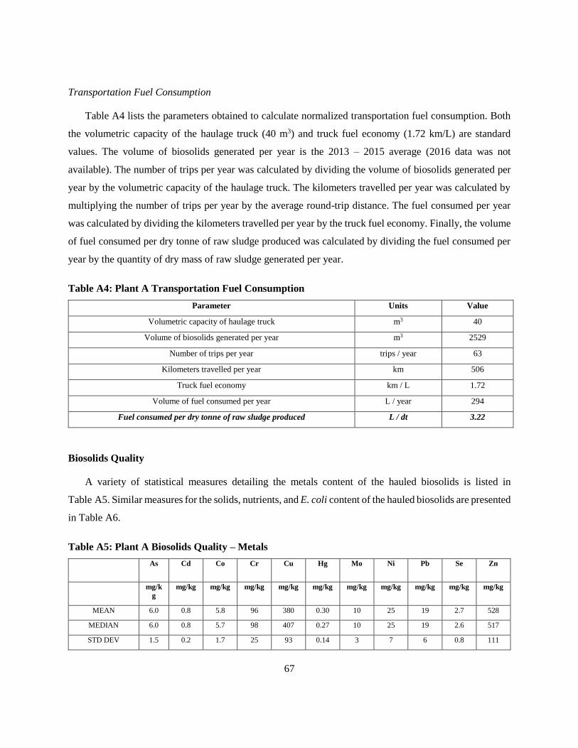
67

Transportation Fuel Consumption

Table A4 lists the parameters obtained to calculate normalized transportation fuel consumption. Both

the volumetric capacity of the haulage truck (40 m3) and truck fuel economy (1.72 km/L) are standard

values. The volume of biosolids generated per year is the 2013 – 2015 average (2016 data was not

available). The number of trips per year was calculated by dividing the volume of biosolids generated per

year by the volumetric capacity of the haulage truck. The kilometers travelled per year was calculated by

multiplying the number of trips per year by the average round-trip distance. The fuel consumed per year

was calculated by dividing the kilometers travelled per year by the truck fuel economy. Finally, the volume

of fuel consumed per dry tonne of raw sludge produced was calculated by dividing the fuel consumed per

year by the quantity of dry mass of raw sludge generated per year.

Table A4: Plant A Transportation Fuel Consumption

Parameter Units Value

Volumetric capacity of haulage truck m3 40

Volume of biosolids generated per year m3 2529

Number of trips per year trips / year 63

Kilometers travelled per year km 506

Truck fuel economy km / L 1.72

Volume of fuel consumed per year L / year 294

Fuel consumed per dry tonne of raw sludge produced L / dt 3.22

Biosolids Quality

A variety of statistical measures detailing the metals content of the hauled biosolids is listed in

Table A5. Similar measures for the solids, nutrients, and E. coli content of the hauled biosolids are presented

in Table A6.

Table A5: Plant A Biosolids Quality – Metals

As Cd Co Cr Cu Hg Mo Ni Pb Se Zn

mg/k

g

mg/kg mg/kg mg/kg mg/kg mg/kg mg/kg mg/kg mg/kg mg/kg mg/kg

MEAN 6.0 0.8 5.8 96 380 0.30 10 25 19 2.7 528

MEDIAN 6.0 0.8 5.7 98 407 0.27 10 25 19 2.6 517

STD DEV 1.5 0.2 1.7 25 93 0.14 3 7 6 0.8 111

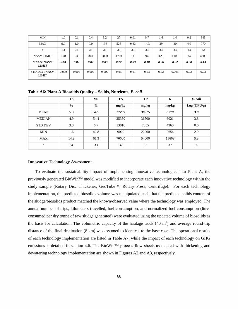
68

MIN 1.0 0.1 0.4 5.2 27 0.01 0.7 1.6 1.0 0.2 345

MAX 9.0 1.0 9.0 136 525 0.62 14.3 39 30 4.0 770

n 33 33 33 33 33 33 33 33 33 33 32

NASM LIMIT 170 34 340 2800 1700 11 94 420 1100 34 4200

MEAN÷NASM

LIMIT

0.04 0.02 0.02 0.03 0.22 0.03 0.10 0.06 0.02 0.08 0.13

STD DEV÷NASM

LIMIT

0.009 0.006 0.005 0.009 0.05 0.01 0.03 0.02 0.005 0.02 0.03

Table A6: Plant A Biosolids Quality – Solids, Nutrients, E. coli

TS VS TN TP K E. coli

% % mg/kg mg/kg mg/kg Log (CFU/g)

MEAN 5.8 54.5 27209 36925 8779 3.9

MEDIAN 4.9 54.4 25350 36500 6021 3.8

STD DEV 3.0 6.7 13016 7855 4963 0.6

MIN 1.6 42.8 9000 22900 2654 2.9

MAX 14.3 65.3 70000 54000 19608 5.3

n 34 33 32 32 37 35

Innovative Technology Assessment

To evaluate the sustainability impact of implementing innovative technologies into Plant A, the

previously generated BioWin™ model was modified to incorporate each innovative technology within the

study sample (Rotary Disc Thickener, GeoTube™, Rotary Press, Centrifuge). For each technology

implementation, the predicted biosolids volume was manipulated such that the predicted solids content of

the sludge/biosolids product matched the known/observed value where the technology was employed. The

annual number of trips, kilometers travelled, fuel consumption, and normalized fuel consumption (litres

consumed per dry tonne of raw sludge generated) were evaluated using the updated volume of biosolids as

the basis for calculation. The volumetric capacity of the haulage truck (40 m3) and average round-trip

distance of the final destination (8 km) was assumed to identical to the base case. The operational results

of each technology implementation are listed in Table A7, while the impact of each technology on GHG

emissions is detailed in section 4.6. The BioWin™ process flow sheets associated with thickening and

dewatering technology implementation are shown in Figures A2 and A3, respectively.

69

Table A7: Plant A Innovative Technology Assessment

Units Base Case Rotary Disc

Thickener

GeoTube™ Rotary

Press

Centrifuge

TSS of product, per BioWin %

4.5 9.1 16.7 22.3

Volumetric capacity of truck m3 40 40 40 40 40

Volume per year m3 2529 2008 803 438 329

Number of trips per year trips / year 63 50 20 11 8

Kilometers travelled per year km 506 402 161 88 66

Truck fuel economy km / L 1.72 1.72 1.72 1.72 1.72

Fuel consumed per year L / year 294 233 93 51 38

Fuel consumed per dry tonne

of raw sludge generated

L / dt 3.22 2.55 1.02 0.56 0.42

Figure A2: Plant A Thickening New Tech PFD

Figure A3: Plant A Dewatering New Tech PFD

70

Appendix B

Plant B Summary

Overview

Plant B is a conventional activated sludge WWTP located in Southern Ontario and operated by Veolia.

Sludge is stabilized via aerobic digestion and the biosolids are stored in an off-site lagoon (no on-site

storage). During spreading season, the biosolids are hauled and applied to land for agricultural purposes.

BioWin Modelling



and the corresponding mean observed value (where applicable) is shown in Table B1. The two observed

MLSS values correspond to each train of liquid treatment. The model process flow sheet is shown in Figure

B1. The model outputs were generally consistent with reported values.

Table B1: Plant B BioWin Model Results


(2014-2016)

MLSS mg/L 3553 3490, 3441


Dry mass of solids returned per day (digester decant) kg TSS/d 158 --





Volume of biosolids generated per day m3 37.1 37.1


VSS content of hauled biosolids % 64 65

Dry mass of biosolids generated per day kg/d 474 586

71

Figure B1: Plant B BioWin Model PFD

Uncertainty

To estimate the uncertainty in raw sludge production, the standard deviation of reported raw sludge

production (228 dry kg/d) was divided by the mean reported sludge production (856 dry kg/d) and converted

to a percentage. Using this measure, the uncertainty was determined to be 27% (sample size, n = 191).

Energy



consumption for each motor of interest (Table B2). The plant does not employ dedicated digester blowers,

therefore, the percentage of air flow to the digester (obtained from plant records) was used to allocate the

fraction of blower electricity consumed by the digester. The total draw for each category of equipment

(stabilization, pumping) was calculated and divided by mass of raw sludge generated daily (Table B3).

Digester electricity consumption was also divided by the daily quantity of VSS destruction to obtain a

measure of energy efficiency (Table B3).

Table B2: Plant B Energy Measurements

Category/Motor Voltag

e (V)

Curren

t (A)

Power

Factor (PF)

Power

Draw (kW)

Motor

Run-Time

(Hr/d)

Daily Electricity

Consumption

(kWh/d)

Stabilization

Blower 1 (aeration + digester) 604 101.3 0.839 91.4 24 2194

Blower 2 (aeration + digester) 604 105 0.838 94.2 24 2261

Sub-total (42% to digester) 1871

72

Pumping

WAS Pump 1 604 1.8 0.7 1.3 1.8 2.3

WAS Pump 2 605 1.9 0.7 1.4 1.6 2.2

Primary pump 1 604 5.0 0.806 4.4 0.35 1.5

Primary pump 2 604 5.1 0.817 4.5 0.27 1.2

Biosolids loading pump 603 7.1 0.81 6.2 0.381 2.4

Sub-total 9.6

Total 1881

Table B3: Plant B Normalized Electricity Consumption


Stabilization 2.72

Pumping 0.01

Total 2.73

Digester Efficiency 8.6 (kWh / kg VSS destroyed)

Chemical Usage

Plant B does not employ the use of chemicals for its sludge handling process.



Plant B transported biosolids from the WWTP to a storage lagoon and then to various fields during

spreading season. Some biosolids were also transported directly from the WWTP to various fields. Based

on plant records, the weighted average round-trip distance the biosolids travelled during 2014 – 2016 was

61 km. The measure accounts for the fact that a smaller volume of biosolids is transported from the lagoon

to the fields due to gravity thickening at the lagoon.


Table B4 lists the parameters obtained to calculate normalized transportation fuel consumption. Both


73

values. The volume of biosolids generated per year is the 2014 – 2016 average. The number of trips per

year was calculated by dividing the volume of biosolids generated per year by the volumetric capacity of

the haulage truck. The kilometers travelled per year was calculated by multiplying the number of trips per

year by the average round-trip distance. The fuel consumed per year was calculated by dividing the

kilometers travelled per year by the truck fuel economy. Finally, the volume of fuel consumed per dry tonne

of raw sludge produced was calculated by dividing the fuel consumed per year by the quantity of dry mass

of raw sludge generated per year.

Table B4: Plant B Transportation Fuel Consumption









Biosolids Quality


Table B5. Similar measures for the solids, nutrients, and E. coli content of the hauled biosolids are presented

in Table B6.

Table B5: Plant B Biosolids Quality – Metals

As Cd Cr Co Cu Pb Hg Mo Ni Se Zn

mg/kg mg/kg mg/kg mg/kg mg/kg mg/kg mg/kg mg/kg mg/kg mg/kg mg/kg

MEAN 7.8 1.8 17 2.8 292 10 N/A 8.1 13 3.9 464

MEDIAN 5.1 0.9 18 1.9 316 11 N/A 7.3 13 3.7 471

STD DEV 5.8 1.5 6.3 1.9 98 4.8 N/A 3.4 5.8 2.3 162

MIN 0.6 0.3 2.2 0.1 30 1.0 N/A 1.3 1.6 0.6 53

MAX 17 4.1 26 5.8 381 17 N/A 14 22 8.2 682

n 11 11 11 11 11 11 11 11 11 7 11

NASM

LIMIT 170 34 2800 340 1700 1100 11 94 420 34 4200

74

AVG÷NASM

LIMIT

0.05 0.05 0.01 0.01 0.17 0.01 All but one

value below

detection limit

0.09 0.03 0.11 0.11

STD

DEV÷NASM

LIMIT

0.03 0.04 0.002 0.006 0.06 0.004 N/A 0.04 0.01 0.07 0.04

Table B6: Plant B Biosolids Quality – Solids, Nutrients, E. coli


(%) (%) mg/kg mg/kg mg/kg Log (CFU/g)

MEAN 1.7 67.1 45630 28497 4001 5.2

MEDIAN 1.6 67.9 53183 28875 4356 5.2

STD DEV 0.7 3.7 24078 9121 1389 0.5

MIN 0.2 53.2 31 3188 754 4.5

MAX 3.7 72.7 69330 37021 5553 6.6

n 50 50 11 11 11 36


To evaluate the sustainability impact of implementing innovative technologies into Plant B, the









of each technology implementation are listed in Table B7, while the impact of each technology on GHG


dewatering technology implementation are shown in Figures B2 and B3, respectively.

75

Table B7: Plant B Innovative Tech Assessment Results

Units Base

Case

Rotary

Disc

Thickener

GeoTub

e

Rotary Press Centrifug

e

BioWin TSS %

4.5 9.1 16.9 22.5

Volume per truck m3 40 40 40 40 40

Volume per year m3 13534 5658 1898 1022 767





Fuel consumed per dry tonne of raw

sludge generated

L / dt 51.2 23.6 10.4 7.3 6.4

Figure B2: Plant B Thickening Innovative Tech PFD

Figure B3: Plant B Dewatering Innovative Tech PFD

76

Appendix C

Plant C Summary

Overview

Plant C is a conventional activated sludge WWTP located in Southern Ontario and operated by the

municipality (owner). Normal sludge handling operations consist of aerobic digestion stabilization,

centrifuge dewatering, and trucking to an off-site storage building. During spreading season, the biosolids

are hauled and applied to land for agricultural purposes.

BioWin Modelling



and the corresponding mean observed value (where applicable) is shown in Table C1. The two observed

MLSS values correspond to each train of liquid treatment. The model process flow sheet is shown in

Figure C1. The values predicted by the model were generally consistent with observed values.

Table C1: Plant C BioWin Model Results


(2014-2016)

MLSS mg/L 3200 3169, 3185

Dry mass of sludge wasted per day kg TSS/d 2051 --


decant)

kg TSS/d 820 --


Dry mass of VSS feed to digester per day kg VSS/d 1346 --



Volume of biosolids generated per day m3 3.10 --


VSS content of hauled biosolids % 57.4 67.0


77

Figure C1: Plant C BioWin Model PFD

Uncertainty

Raw sludge production uncertainty was not calculated directly because the solids content of the raw

primary sludge not available. Instead, given that predicted biosolids mass matched the known reported

value (254.6 dt/year vs 254.4 dt/year) if average TS values were employed in the reported value calculation,

all uncertainty was assumed to be associated with variation in TS content. To calculate uncertainty, the

standard deviation in TS content (2.5 %) was divided by the mean TS content (22.5%) and converted to a

percentage. Using this measure, the uncertainty was determined to be 11% (sample size, n = 95).

Energy



consumption for each motor of interest (Table C2). Additional measurements for individual motors within

the biosolids dewatering building are presented in Table C3 (total dewatering building draw is listed in

Table C2). The total draw for each category of equipment (stabilization, pumping, dewatering, odour

control) was calculated and divided by mass of raw sludge generated daily (Table C4). Digester electricity

consumption was also divided by the daily quantity of VSS destruction to obtain a measure of energy

efficiency (Table C4).

78

Table C2: Plant C Power Draw Measurements


(V)

Current

(A)

Power Factor

(PF)

Power Draw

(kW)

Motor Run-

Time (Hr/d)

Daily Electricity

Consumption (kWh/d)

Stabilization

Digester blower 605 91 0.845 83.1 24 1994

Sub-total 1994

Pumping

WAS pump North 607 2.66 0.741 2.16 12 26

WAS pump south 607 2.66 0.741 2.16 12 26

Raw sludge pump 605 9.95 0.638 6.61 1 6.6

Subtotal 59

Dewatering

Dewatering Building 605 24.8 0.756 19.1 5.8 111

Sub-total 111

Odour Control

Biofilter 605 7.5 0.783 6.2 24 149

Sub-total 149

TOTAL 2311

Table C3: Additional Dewatering Energy Measurements

Motor Voltage (V) Current (A) PF kW Hr/d kWh/d

Centrifuge – Both Drives 603 16.3 0.81 12.3 5.8 71

Centrifuge – Back Drive 604 1.2 0.69 0.9 5.8 5

Centrifuge – Main Drive 603 14.4 0.8 11.2 5.8 65

Centrifuge – Grinder 602 2.4 0.75 1.8 5.8 10

Discharge Conveyor 1 602 1.8 N/A 1.5 5.8 9

Discharge Conveyor 2 602 1.8 N/A 1.5 5.8 9

Sludge Feed Pump 602 1.7 0.78 1.2 5.8 7

79

Table C4: Plant C Normalized Electricity Consumption


Stabilization 1.80

Pumping 0.05

Dewatering 0.10

Odour Control 0.13

Total 2.09


Chemical Usage

Plant C uses polymer as part of its mechanical dewatering process. To determine normalized chemical

usage, purchase records of polymer were used in conjunction with the quantity of raw sludge production.

The facility purchases polymer at a rate of $5.00 per kg of polymer. The money spent during the last three

years of fully operational centrifuge usage was used to determine the average mass of polymer used per

year (Table C5). This value was then divided by the mass of raw sludge generated per year (1108 dry kg)

to obtain the normalized polymer usage (7.7 kg polymer/dt).

Table C5: Plant C Chemical Usage

Year Money spent on polymer ($5.00 / kg polymer) Mass of polymer purchased (kg)

2013 $15,893 3179

2014 $7,632 (Centrifuge not running all year) N/A

2015 $15,264 3053

2016 $15,264 3053

Average 3095

kg polymer used per dry tonne of raw sludge generated 7.7 (kg polymer/dt)



Plant C transports biosolids from the WWTP to an off-site storage facility and then to various fields

during spreading season. The weighted average round-trip distance from the storage facility to farms was

40.5 km, while the round-trip distance between the WWTP and storage facility is 42 km. Therefore, the

total average round-trip distance is 82.5 km.

80


Table C6 lists the parameters obtained to calculate normalized transportation fuel consumption. The

capacity (3 wet tonnes) and fuel economy (2.7 km/L) of the truck that hauls biosolids from the WWTP to

the storage facility was obtained from the plant owner. The capacity (40 m3) and fuel economy (1.72 km/L)

of the truck that hauls biosolids from the storage facility to the farms are standard values.

Table C6: Plant C Transportation Fuel Consumption

WWTP to Storage Facility Notes

Wet tonnes per truck 3 wet tonnes Per owner/operator

Wet tonnes per year 1001 wet tonnes 2014 – 2016 average

Number of trips per year 334 trips / year

Kilometers travelled per year 14018 km / year

Truck fuel economy 2.7 km / L Per owner/operator

Fuel consumed per year 5215 L / year

Storage Facility to Farm

Volume per truck 40 m3/truck Standard value

Volume per day (per BioWin) 3.1 m3/d BioWin calculation

Volume per year 1132 m3/year


Kilometers travelled per year 1175 km / year

Truck fuel economy 1.72 km / L Standard value


Total fuel consumed per year 5898 L / year

Fuel consumed per dry tonne of raw sludge generated 14.6 L/dt

Biosolids Quality


Table C7. Similar measures for the solids, nutrients, and E. coli content of the hauled biosolids are presented

in Table C8.

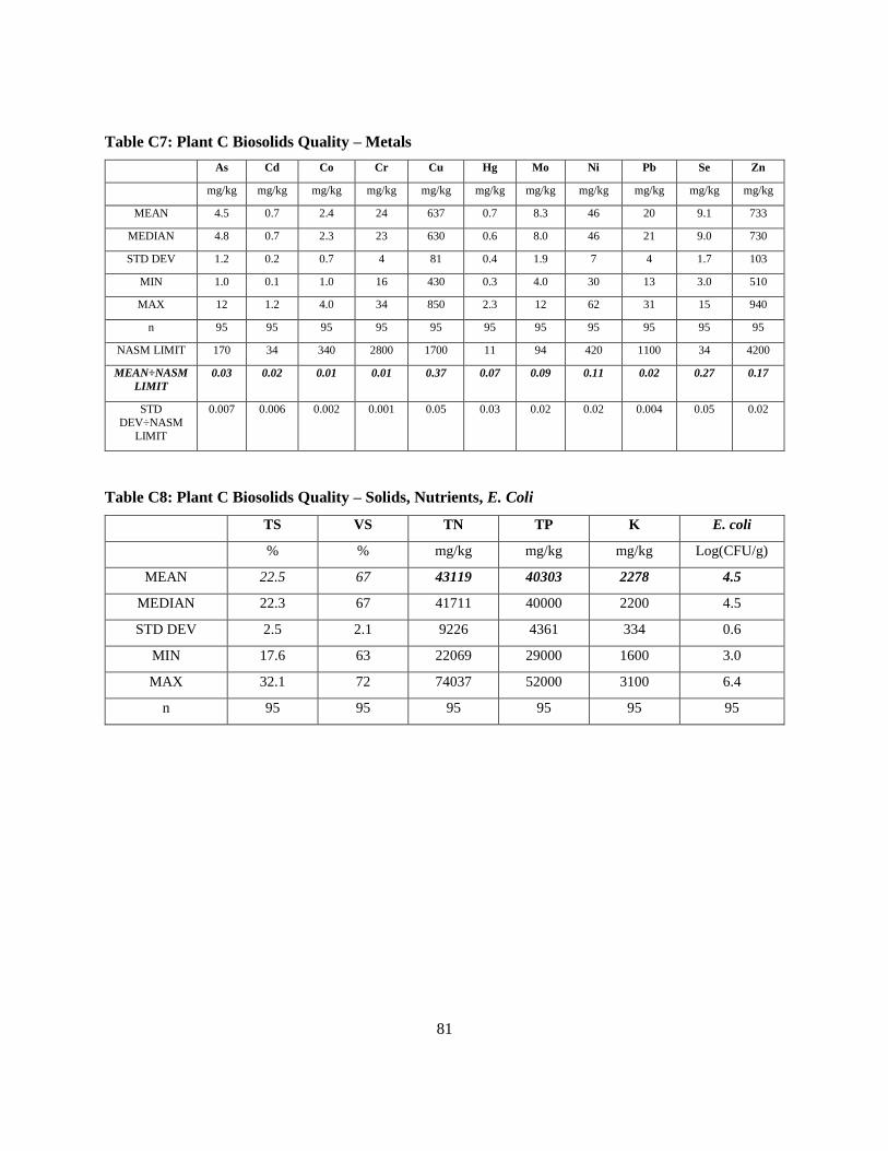
81

Table C7: Plant C Biosolids Quality – Metals



MEAN 4.5 0.7 2.4 24 637 0.7 8.3 46 20 9.1 733

MEDIAN 4.8 0.7 2.3 23 630 0.6 8.0 46 21 9.0 730

STD DEV 1.2 0.2 0.7 4 81 0.4 1.9 7 4 1.7 103

MIN 1.0 0.1 1.0 16 430 0.3 4.0 30 13 3.0 510

MAX 12 1.2 4.0 34 850 2.3 12 62 31 15 940

n 95 95 95 95 95 95 95 95 95 95 95

NASM LIMIT 170 34 340 2800 1700 11 94 420 1100 34 4200

MEAN÷NASM

LIMIT

0.03 0.02 0.01 0.01 0.37 0.07 0.09 0.11 0.02 0.27 0.17

STD

DEV÷NASM

LIMIT

0.007 0.006 0.002 0.001 0.05 0.03 0.02 0.02 0.004 0.05 0.02

Table C8: Plant C Biosolids Quality – Solids, Nutrients, E. Coli


% % mg/kg mg/kg mg/kg Log(CFU/g)

MEAN 22.5 67 43119 40303 2278 4.5

MEDIAN 22.3 67 41711 40000 2200 4.5

STD DEV 2.5 2.1 9226 4361 334 0.6

MIN 17.6 63 22069 29000 1600 3.0

MAX 32.1 72 74037 52000 3100 6.4

n 95 95 95 95 95 95

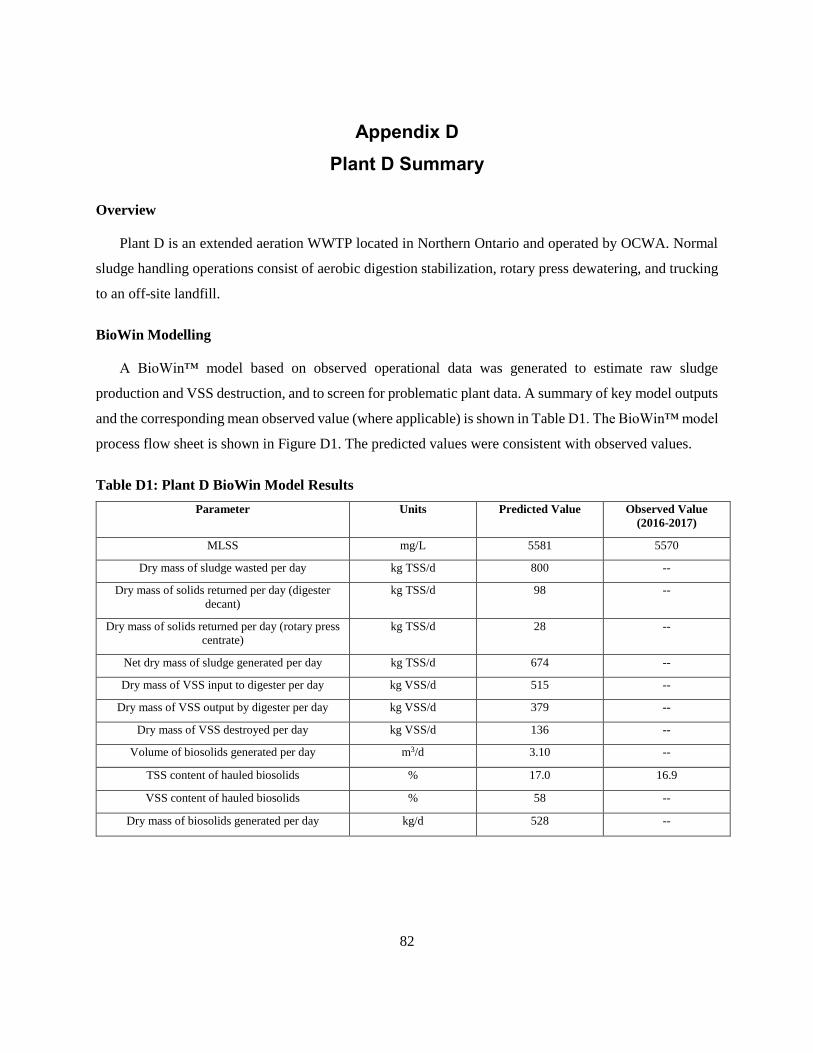
82

Appendix D

Plant D Summary

Overview

Plant D is an extended aeration WWTP located in Northern Ontario and operated by OCWA. Normal

sludge handling operations consist of aerobic digestion stabilization, rotary press dewatering, and trucking

to an off-site landfill.

BioWin Modelling



and the corresponding mean observed value (where applicable) is shown in Table D1. The BioWin™ model

process flow sheet is shown in Figure D1. The predicted values were consistent with observed values.

Table D1: Plant D BioWin Model Results


(2016-2017)

MLSS mg/L 5581 5570



decant)

kg TSS/d 98 --

Dry mass of solids returned per day (rotary press

centrate)

kg TSS/d 28 --





Volume of biosolids generated per day m3/d 3.10 --


VSS content of hauled biosolids % 58 --

Dry mass of biosolids generated per day kg/d 528 --

83

Figure D1: Plant D BioWin Model PFD

Uncertainty

Raw sludge production uncertainty was not calculated directly because the solids content of the waste

sludge not available. As a proxy for raw sludge production, all uncertainty was assumed to be associated

with variation in MLSS concentration (2016 – 2017 data). To calculate uncertainty, the standard deviation

in MLSS concentration (718 mg/L) was divided by the mean MLSS concentration (5570 mg/L) and

converted to a percentage. Using this measure, the uncertainty was determined to be 13% (sample size,

n = 430).

Energy



consumption for each motor of interest (Table D2). The total draw for each category of equipment

(stabilization, pumping, dewatering) was calculated and divided by mass of raw sludge generated daily

(Table D3). Digester electricity consumption was also divided by the daily quantity of VSS destruction to

obtain a measure of energy efficiency (Table D3).

84

Table D2: Plant D Power Draw Measurements


(V)

Current

(A)

Power

Factor (PF)

Power Draw

(kW)

Motor Run-

Time (Hr/d)

Daily Electricity

Consumption (kWh/d)

Stabilization

Digester Blower 596 15.5 0.724 11.8 24 283

Digester Mixer 1 600 19.5 0.989 20.5 24 492

Digester Mixer 2 600 21 0.62 14 8 112

Sub-total 887

Pumping

WAS Pump N/A 4.2 N/A 3.36 4 13

Digester Sludge

Transfer Pump

600 5.7 0.65 2.7 5 14

Sub-total 27

Dewatering

Rotary press 600 6.4 0.772 4.4 5 22

Conveyor 1 N/A N/A N/A 1.5 5 7.5



Lighting + Centrate

Pump

N/A N/A N/A 1 5 5

Sub-total 50

TOTAL 964

Table D3: Plant D Normalized Electricity Consumption

Category Normalized Electricity Consumption

(kWh/dry kg)

Stabilization 1.32

Pumping 0.04

Dewatering 0.07

Total 1.43


85

Chemical Usage

Plant D uses polymer as part of its mechanical dewatering process. To determine normalized polymer

usage, information related to consumption was obtained from the plant operations staff. Polymer is supplied

to the plant in 200 kg drums, each of which contains 90 kg of active polymer (~45% solution). Per

conversations with the operator, the facility uses one drum per week. Per Table D1, the facility generates

674 dry kg of raw sludge per day, which translates to 4.72 dry tonnes per week. The quantity of polymer

used per week (90 kg) was divided by the mass of raw sludge generated per week (4.72 dt) to determine

normalized polymer consumption (19 kg polymer/dt). The results are summarized in Table D4.

Table D4: Plant D Polymer Usage

Parameter Value

kg polymer per drum 90

Number of polymer drums used per week 1

kg polymer used per week 90

dry tonnes raw sludge per week 4.72

kg polymer per dry tonne of raw sludge generated 19



Plant D transports its biosolids to a landfill year-round. The landfill is 4.6 km from the WWTP, hence

the weighted average round-trip distance is 9.2 km.


Since the rotary press practice commenced in 2016, an average of 10.7 bins of biosolids were

transported to the landfill per month. The number therefore represented the number of trips per month,

which projected to 129 trips per year. The fuel economy of the haulage truck (5 km/L) was provided by the

owner. The kilometers travelled per year was calculated by multiplying the number of trips per year by the

round-trip distance (9.2 km). The fuel consumed per year was calculated by dividing the kilometers

travelled per year by the truck fuel economy. Finally, the fuel consumed per dry tonne of raw sludge

produced was calculated by dividing the fuel consumed per year by the quantity of raw sludge produced

(246 dt) per year. The results are presented in Table D5.

86

Table D5: Plant D Transportation Fuel Consumption


Kilometers travelled per year 1184 km

Truck fuel economy 5 km / L


Fuel consumed per dry tonne of raw sludge generated 0.96 L / dt

Biosolids Quality


Table D6. Similar measures for the solids, nutrients, and E. coli content of the hauled biosolids are presented

in Table D7.

Table D6: Plant D Biosolids Quality – Metals



MEAN 5.6 0.47 1.7 13 236 0.6 3.4 9.2 10 2.6 333

MEDIAN 5.5 0.46 1.7 13 236 0.6 3.4 9.2 10 2.7 332

STD DEV 0.7 0.03 0.1 1.3 5 0.1 0.2 0.3 0.4 0.1 12

MIN 4.8 0.4 1.6 12 231 0.6 3.2 8.9 9.2 2.3 322

MAX 6.6 0.5 1.9 15 245 0.7 3.6 9.6 10 2.7 355

n 6 6 6 6 6 6 6 6 6 6 6

NASM LIMIT 170 34 340 2800 1700 11 94 420 1100 34 4200

AVG÷NASM

LIMIT

0.03 0.01 0.005 0.005 0.14 0.06 0.04 0.02 0.009 0.08 0.08

STD DEV÷NASM

LIMIT

0.004 0.001 0.000 0.000 0.003 0.008 0.002 0.001 0.0003 0.004 0.003

Table D7: Plant D Biosolids Quality – Solids, Nutrients, E. coli

VS TS TN TP K E. coli

% % mg/kg mg/kg mg/kg log (CFU/g)

MEAN 76.1 16.9 68192 18800 3563 2.7

MEDIAN 76.3 16.9 67518 18350 3590 2.7

STD DEV 0.7 0.4 3725 1430 113 0.2

MIN 75.1 16.3 63000 17200 3370 2.4

MAX 76.7 17.3 74200 20800 3680 3.0

n 6 6 6 6 6 6

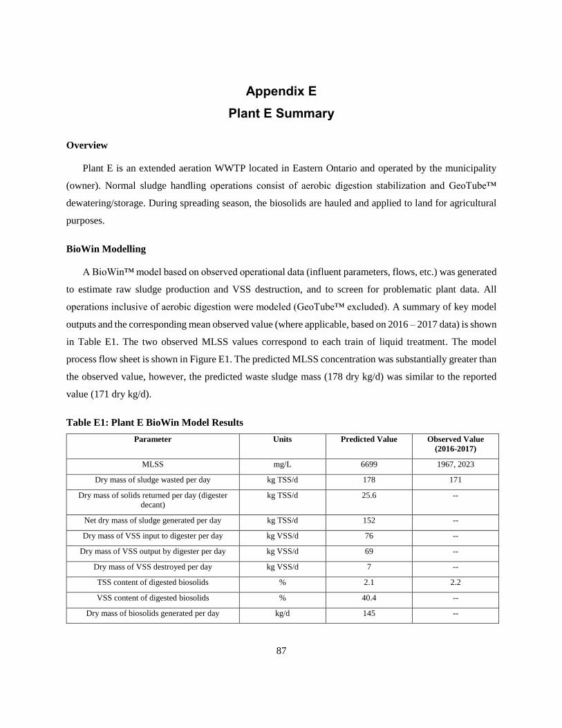
87

Appendix E

Plant E Summary

Overview

Plant E is an extended aeration WWTP located in Eastern Ontario and operated by the municipality

(owner). Normal sludge handling operations consist of aerobic digestion stabilization and GeoTube™

dewatering/storage. During spreading season, the biosolids are hauled and applied to land for agricultural

purposes.

BioWin Modelling

A BioWin™ model based on observed operational data (influent parameters, flows, etc.) was generated

to estimate raw sludge production and VSS destruction, and to screen for problematic plant data. All

operations inclusive of aerobic digestion were modeled (GeoTube™ excluded). A summary of key model

outputs and the corresponding mean observed value (where applicable, based on 2016 – 2017 data) is shown

in Table E1. The two observed MLSS values correspond to each train of liquid treatment. The model

process flow sheet is shown in Figure E1. The predicted MLSS concentration was substantially greater than

the observed value, however, the predicted waste sludge mass (178 dry kg/d) was similar to the reported

value (171 dry kg/d).

Table E1: Plant E BioWin Model Results


(2016-2017)

MLSS mg/L 6699 1967, 2023



decant)

kg TSS/d 25.6 --





TSS content of digested biosolids % 2.1 2.2

VSS content of digested biosolids % 40.4 --


88

Figure E1: Plant E BioWin Model PFD

Uncertainty


production was divided by the mean reported sludge production and converted to a percentage. Using

reported WAS TSS values in conjunction with daily WAS volumes, the calculated uncertainty was 96%.

However, the operator reported that WAS TSS varied substantially depending on the sampling technique,

and therefore recommended that a constant TSS content of 13,000 mg/L be employed in the calculation.

Using this measure, the daily sludge production mean and standard deviation was 171 and 59 dry kg/d,

respectively. The resulting uncertainty was determined to be 34% (sample size, n = 122).

Energy



consumption for each motor of interest (Table E2). The total draw for each category of equipment

(stabilization, pumping) was calculated and divided by mass of raw sludge generated daily (Table E3).

Digester electricity consumption was also divided by the daily quantity of VSS destruction to obtain a

measure of energy efficiency (Table E3).

89

Table E2: Plant E Energy Measurements


(V)

Current

(A)

Power Factor

(PF)

Power Draw

(kW)

Motor Run -

Time (Hr/d)

Daily Electricity

Consumption (kWh/d)

Stabilization

Digester blower 627 20.1 0.787 16.4 24 394

Sub-total 394

Pumping

WAS pump 627 1.6 0.755 1.3 12 16

Sub-total 16

TOTAL 410

Table E3: Plant E Normalized Electricity Consumption


Stabilization 2.59

Pumping 0.10

Total 2.69

Digester Efficiency 56 (kWh / kg VSS destroyed)

Chemical Usage

Plant E uses polymer as part of its GeoTube™ dewatering process. The operator reported that a

110 mg/L solution of polymer was dosed into a sludge feed concentration of 12000 mg/L, which

corresponded to a 0.0092 dt polymer/dt raw sludge ratio. Converting the numerator into kg yields a

normalized polymer usage of 9.2 kg polymer/dt.



Plant E transports biosolids from the WWTP to agricultural farms during spreading season. The

weighted average round-trip distance from the WWTP to the farms between 2016 – 2017 was 53 km.

90


Table E4 lists the parameters obtained to calculate normalized transportation fuel consumption. Both









Table E4: Plant E Transportation Fuel Consumption

Parameter Value Units

Volumetric capacity of haulage truck 40 m3

Volume of biosolids generated per year 584 m3



Truck fuel economy 1.72 km / L

Volume of fuel consumed per year 447 L / year

Fuel consumed per dry tonne of raw sludge produced 8.1 L / dt

Biosolids Quality


Table E5. Similar measures for the solids, nutrients, and E. coli content of the hauled biosolids are presented

in Table E6.

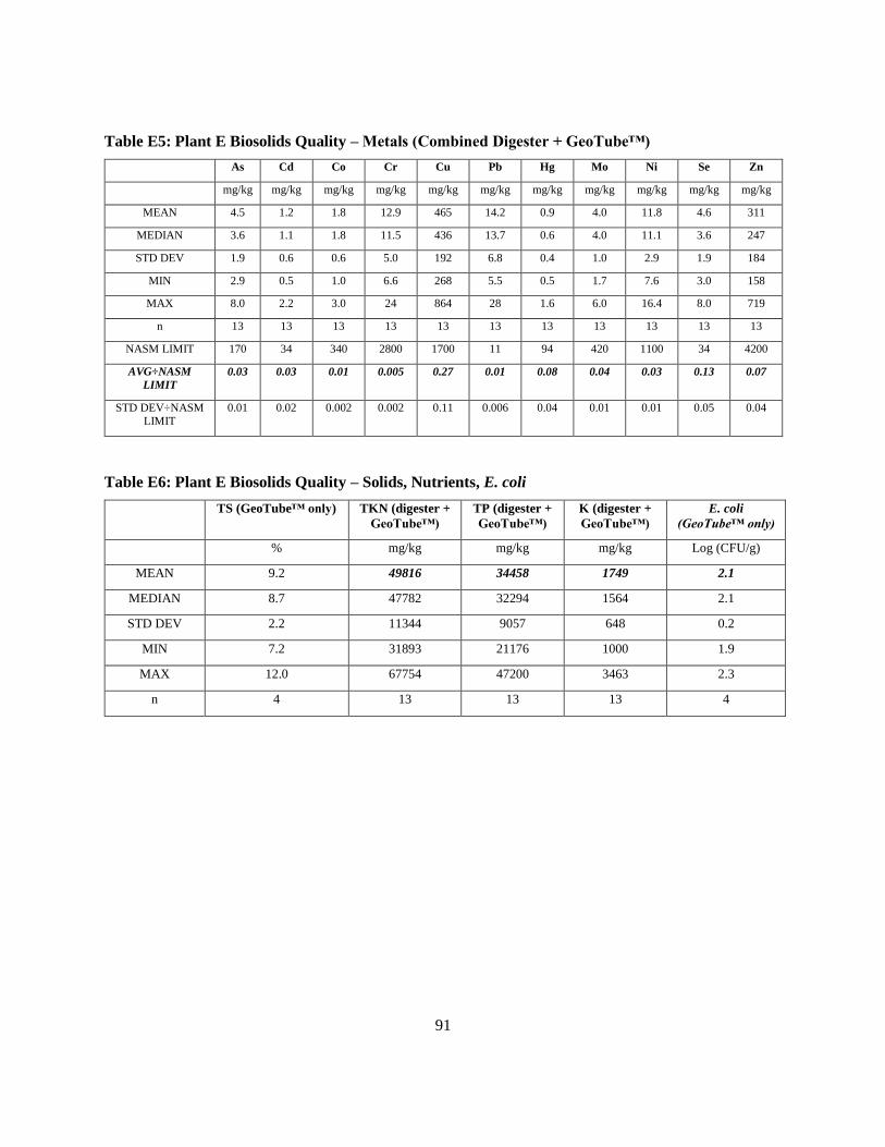
91

Table E5: Plant E Biosolids Quality – Metals (Combined Digester + GeoTube™)

As Cd Co Cr Cu Pb Hg Mo Ni Se Zn


MEAN 4.5 1.2 1.8 12.9 465 14.2 0.9 4.0 11.8 4.6 311

MEDIAN 3.6 1.1 1.8 11.5 436 13.7 0.6 4.0 11.1 3.6 247

STD DEV 1.9 0.6 0.6 5.0 192 6.8 0.4 1.0 2.9 1.9 184

MIN 2.9 0.5 1.0 6.6 268 5.5 0.5 1.7 7.6 3.0 158

MAX 8.0 2.2 3.0 24 864 28 1.6 6.0 16.4 8.0 719

n 13 13 13 13 13 13 13 13 13 13 13

NASM LIMIT 170 34 340 2800 1700 11 94 420 1100 34 4200

AVG÷NASM

LIMIT

0.03 0.03 0.01 0.005 0.27 0.01 0.08 0.04 0.03 0.13 0.07

STD DEV÷NASM

LIMIT

0.01 0.02 0.002 0.002 0.11 0.006 0.04 0.01 0.01 0.05 0.04

Table E6: Plant E Biosolids Quality – Solids, Nutrients, E. coli

TS (GeoTube™ only) TKN (digester +

GeoTube™)

TP (digester +

GeoTube™)

K (digester +

GeoTube™)

E. coli

(GeoTube™ only)

% mg/kg mg/kg mg/kg Log (CFU/g)

MEAN 9.2 49816 34458 1749 2.1

MEDIAN 8.7 47782 32294 1564 2.1

STD DEV 2.2 11344 9057 648 0.2

MIN 7.2 31893 21176 1000 1.9

MAX 12.0 67754 47200 3463 2.3

n 4 13 13 13 4

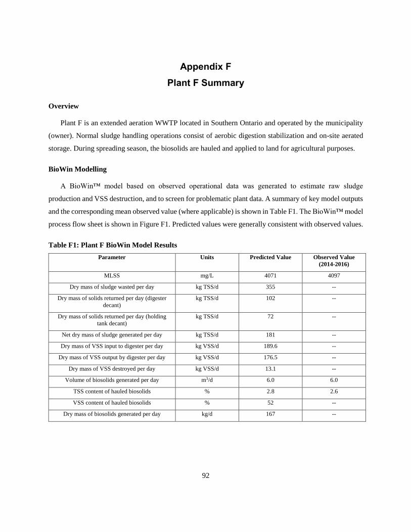
92

Appendix F

Plant F Summary

Overview

Plant F is an extended aeration WWTP located in Southern Ontario and operated by the municipality

(owner). Normal sludge handling operations consist of aerobic digestion stabilization and on-site aerated

storage. During spreading season, the biosolids are hauled and applied to land for agricultural purposes.

BioWin Modelling



and the corresponding mean observed value (where applicable) is shown in Table F1. The BioWin™ model

process flow sheet is shown in Figure F1. Predicted values were generally consistent with observed values.

Table F1: Plant F BioWin Model Results


(2014-2016)

MLSS mg/L 4071 4097



decant)

kg TSS/d 102 --

Dry mass of solids returned per day (holding

tank decant)

kg TSS/d 72 --


Dry mass of VSS input to digester per day kg VSS/d 189.6 --

Dry mass of VSS output by digester per day kg VSS/d 176.5 --

Dry mass of VSS destroyed per day kg VSS/d 13.1 --

Volume of biosolids generated per day m3/d 6.0 6.0




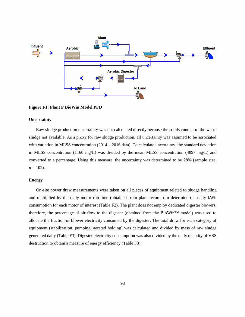
93

Figure F1: Plant F BioWin Model PFD

Uncertainty


sludge not available. As a proxy for raw sludge production, all uncertainty was assumed to be associated

with variation in MLSS concentration (2014 – 2016 data). To calculate uncertainty, the standard deviation



n = 102).

Energy



consumption for each motor of interest (Table F2). The plant does not employ dedicated digester blowers,

therefore, the percentage of air flow to the digester (obtained from the BioWin™ model) was used to

allocate the fraction of blower electricity consumed by the digester. The total draw for each category of

equipment (stabilization, pumping, aerated holding) was calculated and divided by mass of raw sludge

generated daily (Table F3). Digester electricity consumption was also divided by the daily quantity of VSS

destruction to obtain a measure of energy efficiency (Table F3).

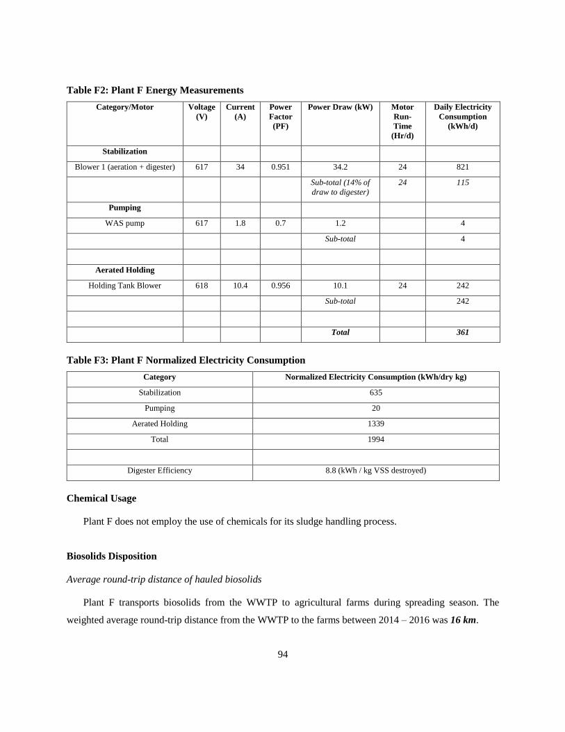
94

Table F2: Plant F Energy Measurements


(V)

Current

(A)

Power

Factor

(PF)

Power Draw (kW) Motor

Run-

Time

(Hr/d)

Daily Electricity

Consumption

(kWh/d)

Stabilization

Blower 1 (aeration + digester) 617 34 0.951 34.2 24 821

Sub-total (14% of

draw to digester)

24 115

Pumping

WAS pump 617 1.8 0.7 1.2 4

Sub-total 4

Aerated Holding

Holding Tank Blower 618 10.4 0.956 10.1 24 242

Sub-total 242

Total 361

Table F3: Plant F Normalized Electricity Consumption


Stabilization 635

Pumping 20

Aerated Holding 1339

Total 1994


Chemical Usage

Plant F does not employ the use of chemicals for its sludge handling process.



Plant F transports biosolids from the WWTP to agricultural farms during spreading season. The


95


Table F4 lists the parameters obtained to calculate normalized transportation fuel consumption. Both









Table F4: Plant F Transportation Fuel Consumption








Biosolids Quality

A variety of statistical measures detailing the metals content of the hauled biosolids is listed in Table F5.

Similar measures for the solids, nutrients, and E. coli content of the hauled biosolids are presented in

Table F6.

Table F5: Plant F Biosolids Quality – Metals



MEAN 4.7 0.5 2.0 24 538 0.9 5.5 13 29 6.9 528

MEDIAN 4.3 0.5 1.9 20 505 0.7 5.4 13 27 6.1 546

STD DEV 1.4 0.2 0.4 11 112 0.5 2.0 3 8 2.5 121

MIN 2.9 0.18 1.5 13 407 0.01 2.6 9.4 16 4.1 325

MAX 7.5 0.73 2.6 51 797 1.8 2.6 18 47 11 773

96

n 11 11 11 11 11 11 11 11 11 11 11

NASM LIMIT 170 34 340 2800 1700 11 94 420 1100 34 4200

AVG÷NASM

LIMIT

0.03 0.01 0.01 0.01 0.32 0.08 0.06 0.03 0.03 0.20 0.13

STD

DEV÷NASM

LIMIT

0.01 0.005 0.001 0.004 0.07 0.05 0.02 0.01 0.01 0.07 0.03

Table F6: Plant F Biosolids Quality – Solids, Nutrients, E. coli

TS TN TP K E. coli


MEAN 2.6 38359 32355 2180 4.3

MEDIAN 2.5 36621 31937 1951 4.7

STD DEV 0.6 11756 4428 490 1.1

MIN 1.7 20508 25610 1774 2.6

MAX 3.8 65523 41802 2978 5.4

n 11 10 11 5 11


To evaluate the sustainability impact of implementing innovative technologies into Plant F, the









of each technology implementation are listed in Table F7, while the impact of each technology on GHG


dewatering technology implementation are shown in Figures F2 and F3, respectively.

97

Table F7: Plant F Innovative Tech Assessment Results

Base Case Disc

Thickener

GeoTube Fournier

Press

Centrifuge

BioWin TSS %

4.5 9.0 17.0 22.7


Volume per year m3 2190 1497 694 365 274





Fuel consumed / dt sludge L / dt 7.8 5.3 2.5 1.3 0.97

Figure F2: Plant F Thickening Innovative Tech PFD

Figure F3: Plant F Dewatering Innovative Tech PFD

98

Appendix G

Plant G Summary

Overview

Plant G is an extended aeration WWTP located in Southern Ontario and operated by the municipality

(owner). Normal sludge handling operations consist of aerobic digestion stabilization and on-site aerated

storage. During spreading season, the biosolids are hauled and applied to land for agricultural purposes.

BioWin Modelling



and the corresponding mean observed value (where applicable) is shown in Table G1. The three observed


Figure G1. The predicted values were generally consistent with observed values.

Table G1: Plant G BioWin Model Results


(2014-2016)

MLSS mg/L 7480 8078, 6720, 7206



decant)

kg TSS/d 151 --





Volume of biosolids generated per day m3/d 15 --


VSS content of hauled biosolids % 59 67

99

Figure G1: Plant G BioWin Model PFD

Uncertainty


sludge was not available. As a proxy for raw sludge production, all uncertainty was assumed to be

associated with variation in MLSS concentration. Given that the plant employs multiple liquid treatment

trains (and thus exhibits multiple MLSS concentrations), the uncertainty was calculated for each train and

the highest value was used in subsequent KPI calculations. To calculate uncertainty, the standard deviation



n = 64).

Energy



consumption for each motor of interest (Table G2). The plant does not employ dedicated digester blowers;

one blower services both the digesters and holding tank. An analysis of air flow data from 2016–2017

revealed that 98% of the sludge blower air serviced the digesters, while 2% serviced the holding tank.

Therefore, 98% of the electricity associated with blower operation was allocated to digester operation, while

2% was allocated to aerated holding tank operation. The total draw for each category of equipment

(stabilization, pumping, aerated holding) was calculated and divided by mass of raw sludge generated daily

(Table G3). Digester electricity consumption was also divided by the daily quantity of VSS destruction to

obtain a measure of energy efficiency (Table G3).

100

Table G2: Plant G Energy Measurements


(V)

Current

(A)

Power Factor

(PF)

Power Draw

(kW)

Motor Run-

Time (Hr/d)

Daily Electricity

Consumption

(kWh/d)

Stabilization

Blower (digester +

aerated holding tank)

605 45.2 0.8 37 24 888

Sub-total (98% to digester) 870

Pumping

WAS Pump 607 7.1 0.778 6.5 1.8 11.7

Sub-total 11.7

Aerated Holding

Blower (digester +

aerated holding tank)

605 45.2 0.8 37 24 888

Sub-total (2% to aerated holding

tank)

18

Total 900

Table G3: Plant G Normalized Electricity Consumption


Stabilization 2.27

Pumping 0.03

Aerated Holding 0.04

Total 2.34


Chemical Usage

Plant G does not employ the use of chemicals for its sludge handling process.



Plant F transports biosolids from the WWTP to agricultural farms during spreading season. The


101


Table G4 lists the parameters obtained to calculate normalized transportation fuel consumption. Both









Table G4: Plant G Transportation Fuel Consumption









Biosolids Quality


Table G5. Similar measures for the solids, nutrients, and E. coli content of the hauled biosolids are presented

in Table G6.

Table G5: Plant G Biosolids Quality – Metals



MEAN 5.3 0.6 4.6 17 496 0.3 5.6 13 88 4.7 385

MEDIAN 4.8 0.6 4.6 16 506 0.2 5.5 14 66 4.5 369

STD DEV 2.1 0.3 0.9 4 78 0.2 1.3 3 65 1.3 102

MIN 0.6 0.07 2.4 9.4 315 0.08 3.7 4.1 17 2.1 176

MAX 12 1.4 6.5 27 643 1.3 9.4 20 304 7.8 585

102

n 32 32 32 32 32 32 32 32 32 32 32

NASM LIMIT 170 34 340 2800 1700 11 94 420 1100 34 4200

AVG÷NASM

LIMIT

0.03 0.02 0.01 0.01 0.29 0.02 0.06 0.03 0.08 0.14 0.09

STD DEV÷NASM

LIMIT

0.01 0.01 0.003 0.001 0.05 0.02 0.01 0.007 0.06 0.04 0.02

Table G6: Plant G Biosolids Quality – Solids, Nutrients, E. coli


% % mg/kg mg/kg mg/kg Log (CFU/g)

MEAN 2.4 67 49759 29908 3341 4.4

MEDIAN 2.3 67 49527 30154 3189 4.5

STD DEV 0.7 3 10397 4159 630 0.6

MIN 1.3 58 20782 21176 2180 2.9

MAX 4.9 74 83914 38554 4661 5.5

n 33 33 32 32 32 32

Innovative Tech Assessment

To evaluate the sustainability impact of implementing innovative technologies into Plant G, the









of each technology implementation are listed in Table G7, while the impact of each technology on GHG


dewatering technology implementation are shown in Figures G2 and G3, respectively.

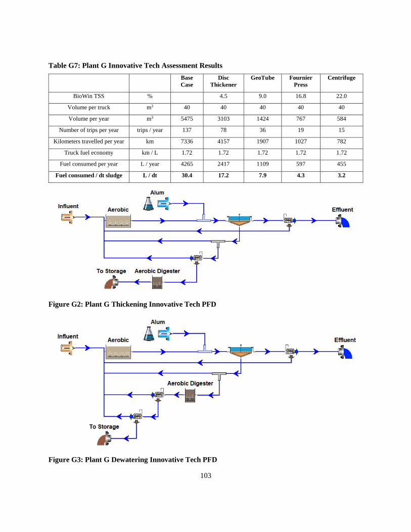
103

Table G7: Plant G Innovative Tech Assessment Results

Base

Case

Disc

Thickener

GeoTube Fournier

Press

Centrifuge

BioWin TSS %

4.5 9.0 16.8 22.0


Volume per year m3 5475 3103 1424 767 584





Fuel consumed / dt sludge L / dt 30.4 17.2 7.9 4.3 3.2

Figure G2: Plant G Thickening Innovative Tech PFD

Figure G3: Plant G Dewatering Innovative Tech PFD

104

Appendix H

Plant H Summary

Overview

Plant H is an extended aeration WWTP located in Southern Ontario and operated by the municipality

(owner). Normal sludge handling operations consist of aerated holding, centrifuge dewatering (upstream),

thermo-alkali hydrolysis stabilization, and on-site storage. During spreading season, the biosolids are

hauled and applied to land for agricultural purposes.

BioWin Modelling


production and VSS destruction, and to screen for problematic plant data. All operations inclusive of

centrifuge dewatering were incorporated in the model. The thermo-alkali reactor was not modeled. A

summary of key model outputs and the corresponding mean observed value (where applicable) is shown in

Table H1. The BioWin™ model process flow sheet is shown in Figure H1. The predicted values were

consistent with observed values.

Table H1: Plant H BioWin Model Results


(2015-2017)

MLSS mg/L 5469 5525



decant)

kg TSS/d 674 --

Dry mass of solids returned per day (centrifuge

centrate)

kg TSS/d 14 --


TSS content of sludge (centrifuge product) % 17.2% 16.9%

Dry mass of biosolids generated per day kg/d 274 kg/d 274 kg/d

105

Figure H1: Plant H BioWin Model PFD

Uncertainty


production (306 dry kg/d) was divided by the mean reported sludge production (1094 dry kg/d) and

converted to a percentage. Using this measure, the uncertainty was determined to be 28% (sample

size, n = 339).

Electricity



consumption for each motor of interest (Table H2). The total draw for each category of equipment

(stabilization, pumping) was calculated and divided by mass of raw sludge generated daily (Table H3).

Table H2: Plant H Energy Measurements


(V)

Current

(A)

Power Factor

(PF)

Power

Draw (kW)

Motor Run-

Time (Hr/d)

Daily Electricity

Consumption (kWh/d)

Stabilization

Reactor (all) 605 38.1 0.803 34.4 2 69

Sub-total 69

Pumping

WAS pump 606 2.5 0.652 1.7 4 7

Sludge loading pump 604 25.6 0.96 26 0.14 4

Sub-total 11

106

Dewatering

Centrifuge (all) 606 10.3 0.841 9.1 1.5 14

Sludge transfer pump 606 1.8 0.734 1.5 1.5 2

Sub-total 16

Aerated Holding

Blower 1 605 26.6 0.809 24.9 4.8 119

Blower 2 605 26.6 0.809 24.9 4.5 111

Blower 3 604 11.3 0.852 10.5 11.4 119

Sub-total 349

Odour Control

Sludge Building

BioRem

605 11 0.833 9.9 24 238

Reactor BioRem 606 9.7 0.85 8.1 4 32

Sub-total 270

TOTAL 715

Table H3: Plant H Normalized Electricity Consumption


Stabilization 0.25

Pumping 0.04

Dewatering 0.06

Aerated Holding 1.27

Odour Control 0.98

Total 2.60

Natural Gas

Natural gas is employed as part of the stabilization process at plant H. Its usage was calculated by

subtracting the reported baseline usage (for plant-wide heating) from the total draw reported during

stabilization operation and dividing the difference by the dry mass flow of sludge processed. The usage was

determined to be 0.037 m3/dt.

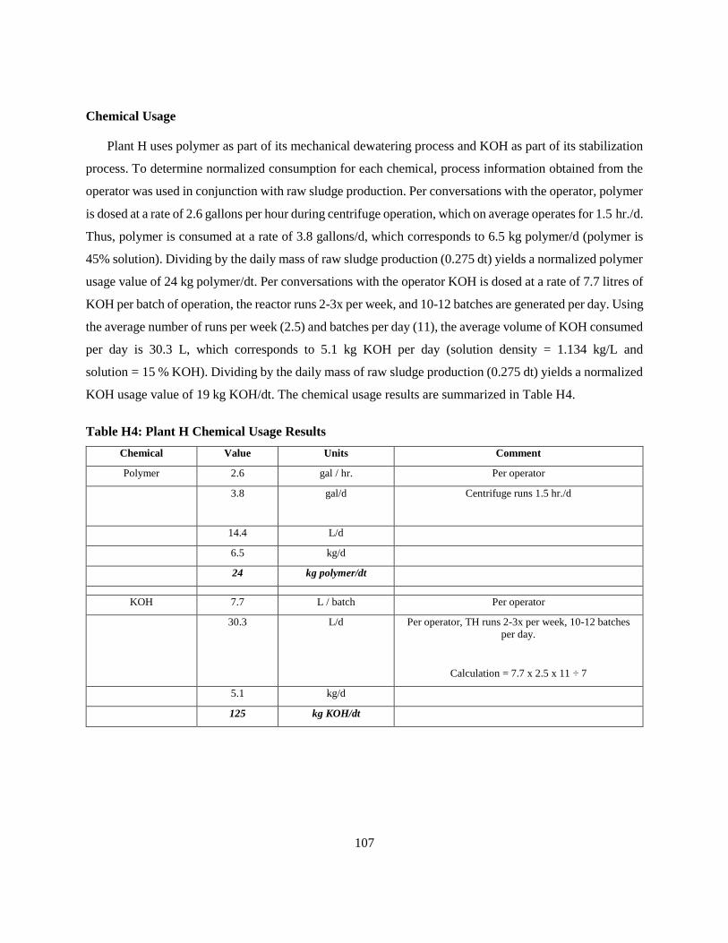
107

Chemical Usage

Plant H uses polymer as part of its mechanical dewatering process and KOH as part of its stabilization

process. To determine normalized consumption for each chemical, process information obtained from the

operator was used in conjunction with raw sludge production. Per conversations with the operator, polymer

is dosed at a rate of 2.6 gallons per hour during centrifuge operation, which on average operates for 1.5 hr./d.

Thus, polymer is consumed at a rate of 3.8 gallons/d, which corresponds to 6.5 kg polymer/d (polymer is

45% solution). Dividing by the daily mass of raw sludge production (0.275 dt) yields a normalized polymer

usage value of 24 kg polymer/dt. Per conversations with the operator KOH is dosed at a rate of 7.7 litres of

KOH per batch of operation, the reactor runs 2-3x per week, and 10-12 batches are generated per day. Using

the average number of runs per week (2.5) and batches per day (11), the average volume of KOH consumed

per day is 30.3 L, which corresponds to 5.1 kg KOH per day (solution density = 1.134 kg/L and

solution = 15 % KOH). Dividing by the daily mass of raw sludge production (0.275 dt) yields a normalized

KOH usage value of 19 kg KOH/dt. The chemical usage results are summarized in Table H4.

Table H4: Plant H Chemical Usage Results

Chemical Value Units Comment

Polymer 2.6 gal / hr. Per operator

3.8 gal/d Centrifuge runs 1.5 hr./d

14.4 L/d

6.5 kg/d

24 kg polymer/dt

KOH 7.7 L / batch Per operator

30.3 L/d Per operator, TH runs 2-3x per week, 10-12 batches

per day.

Calculation = 7.7 x 2.5 x 11 ÷ 7

5.1 kg/d

125 kg KOH/dt

108



Plant H transports its biosolids to agricultural farms during spreading season. During 2016, the first

year the thermo-alkali product was generated, the weighted average round trip distance between the WWTP

and fields was 9.3 km.


Table H5 lists the parameters obtained to calculate normalized transportation fuel consumption. Both


values. The volume of biosolids generated per year is the reported 2016 value. The number of trips per year

was calculated by dividing the volume of biosolids generated per year by the volumetric capacity of the

haulage truck. The kilometers travelled per year was calculated by multiplying the number of trips per year

by the average round-trip distance. The fuel consumed per year was calculated by dividing the kilometers

travelled per year by the truck fuel economy. Finally, the volume of fuel consumed per dry tonne of raw

sludge produced was calculated by dividing the fuel consumed per year by the quantity of dry mass of raw

sludge generated per year.

Table H5: Plant H Fuel Consumption

Volumetric capacity of haulage truck 40 m3

Volume of biosolids generated per year 984 m3



Truck fuel economy 1.72 km / L

Volume of fuel consumed per year 133 L / year

Fuel consumed per dry tonne of raw sludge produced 1.3 L / dt

Biosolids Quality


Table H6. Similar measures for the solids, nutrients, and E. coli content of the hauled biosolids are presented

in Table H7.

109

Table H6: Plant H Biosolids Quality – Metals

Ar Cd Co Cr Cu Hg Mo Ni Pb Se Zn


MEAN 2.9 0.8 3.1 46 550 0.75 13 14 27 3 456

MEDIAN 3.0 0.8 3.1 38 550 0.66 12 15 14 2 448

STD DEV 1.5 0.3 1.4 24 112 0.45 5 4 36 1 124

MIN 1 0 1 14 230 0 6 7 7 1 190

MAX 7 2 6 96 807 3 26 22 160 7 798

n 35 35 35 35 35 33 35 35 35 35 35

NASM LIMIT 170 34 340 2800 1700 11 94 420 1100 34 4200

AVG÷NASM

LIMIT

0.02 0.02 0.01 0.02 0.32 0.07 0.14 0.03 0.02 0.09 0.11

STD DEV÷NASM

LIMIT

0.009 0.01 0.004 0.009 0.07 0.04 0.05 0.01 0.03 0.04 0.03

Table H7: Plant H Biosolids Quality – Solids, Nutrients, E. coli

TS TN TP K E. coli

mg/kg mg/kg mg/kg mg/kg Log (CFU/g)

MEAN 99314 42130 36968 53111 2.1

MEDIAN 100400 39637 35500 53000 2.0

STD DEV 24113 16410 5602 26036 0.28

MIN 11900 12038 28879 8000 1.5

MAX 145000 80428 49381 105263 2.9

n 35 34 32 32 19

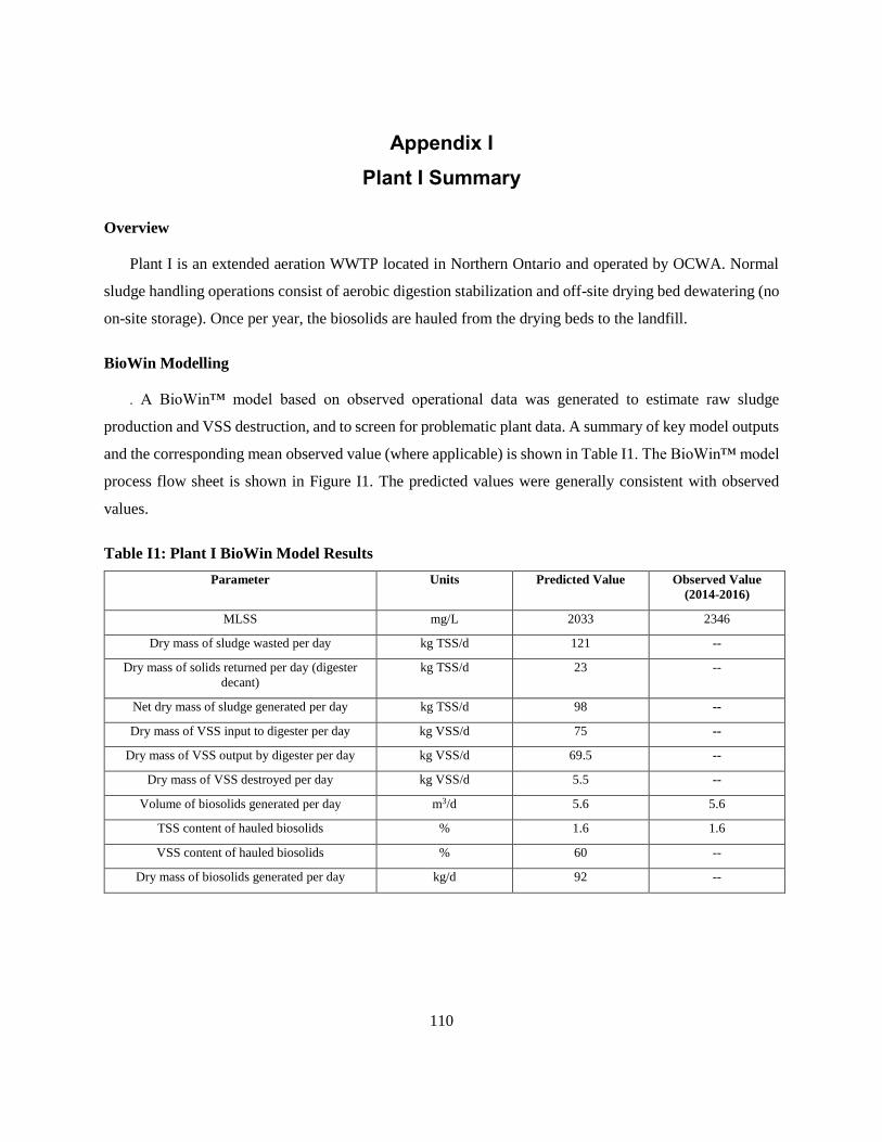
110

Appendix I

Plant I Summary

Overview

Plant I is an extended aeration WWTP located in Northern Ontario and operated by OCWA. Normal

sludge handling operations consist of aerobic digestion stabilization and off-site drying bed dewatering (no

on-site storage). Once per year, the biosolids are hauled from the drying beds to the landfill.

BioWin Modelling

. A BioWin™ model based on observed operational data was generated to estimate raw sludge


and the corresponding mean observed value (where applicable) is shown in Table I1. The BioWin™ model

process flow sheet is shown in Figure I1. The predicted values were generally consistent with observed

values.

Table I1: Plant I BioWin Model Results


(2014-2016)

MLSS mg/L 2033 2346



decant)

kg TSS/d 23 --



Dry mass of VSS output by digester per day kg VSS/d 69.5 --

Dry mass of VSS destroyed per day kg VSS/d 5.5 --

Volume of biosolids generated per day m3/d 5.6 5.6




111

Figure I 1: Plant I BioWin Model PFD

Uncertainty

Raw sludge production uncertainty was not calculated directly because the solids content values of the

waste sludge were limited in number. Instead, given that the biosolid volumes were known, all uncertainty

was assumed to be associated with variation in biosolids TS content. To calculate uncertainty, the standard

deviation in TS content (0.42 %) was divided by the mean TS content (1.64%) and converted to a

percentage. Using this measure, the uncertainty was determined to be 26% (sample size, n = 59).

Energy



consumption for each motor of interest (Table I2). The plant does not employ dedicated digester blowers;

one blower services both the aeration basin and digester. The percentage of air flow to the digester was

assumed to be equal to the percentage of volume the digester utilizes within the treatment unit (14%). The

percentage was then used to allocate the fraction of blower electricity consumption to the digester. The total

draw for each category of equipment (stabilization, pumping) was calculated and divided by mass of raw

sludge generated daily (Table I3). Digester electricity consumption was also divided by the daily quantity

of VSS destruction to obtain a measure of energy efficiency (Table I3).

112

Table I2: Plant I Energy Measurements


(V)

Current

(A)

Power Factor

(PF)

Power

Draw (kW)

Motor Run-

Time (Hr/d)

Daily Electricity

Consumption

(kWh/d)

Stabilization

Blower (aeration + digester) 620 25.2 0.85 17.1 24 410

Sub-total (15% to digester) 61.5

Pumping

WAS/RAS 1* 618 3.2 0.85 3.6 0.25 0.9

WAS/RAS 2* 618 3.2 0.85 3.6 0.25 0.9

Sub-total 1.8

Total 63.3

*6 min/d in winter, 24 min/d summer → 15 min/d overall = 0.25 hr./d

Table I3: Plant I Normalized Electricity Consumption


Stabilization 0.84

Pumping 0.02

Total 0.86


Chemical Usage

Plant I does not employ the use of chemicals for its sludge handling process.



The round-trip distance from the WWTP to the drying bed is 52 km. 182.5 m3 (out of 1856 m3 total) is

eventually transported from the drying bed to the landfill (a round-trip distance of 40 km). The weighted

average round-trip distance of the entire operation is 56 km.


Table I4 lists the parameters obtained to calculate normalized transportation fuel consumption. Both

the volumetric capacity of the haulage truck (16.5 m3) and truck fuel economy (2.0 km/L) were obtained

113

from the plant owner. The volume of biosolids generated per year is the 2014 – 2016 average. The number

of trips per year was calculated by dividing the volume of biosolids generated per year by the volumetric

capacity of the haulage truck. The kilometers travelled per year was calculated by multiplying the number

of trips per year by the average round-trip distance. The fuel consumed per year was calculated by dividing

the kilometers travelled per year by the truck fuel economy. Finally, the volume of fuel consumed per dry

tonne of raw sludge produced was calculated by dividing the fuel consumed per year by the quantity of dry

mass of raw sludge generated per year.

Table I4: Plant I Transportation Fuel Consumption

Volumetric capacity of haulage truck m3 16.5



Number of trips to drying bed per year trips / year 124

Kilometers travelled per year to/from WWTP → drying bed km / year 6917

Volume of fuel consumed per year (WWTP → drying bed) L / year 3459

Volume of fuel consumed per year (drying bed → landfill) km / year 71

Volume of fuel consumed per year (total) L / year 3530

Fuel consumed per dry tonne of raw sludge produced L / dt 99

Biosolids Quality

A variety of statistical measures detailing the metals content of the hauled biosolids is listed in Table I5.


Table I6.

Table I5: Plant I Biosolids Quality – Metals


mg/k

g mg/kg mg/kg mg/kg mg/kg mg/kg mg/kg mg/kg mg/kg mg/kg mg/kg

MEAN 20 0.7 3.4 12 1168 1.0 4.2 16 31 2.5 440

MEDIAN 21 0.8 3.5 12 1137 1.0 4.2 16 30 2.5 453

STD DEV 3 0.1 0.3 2 189 0.1 0.4 2 3 0.3 78

MIN 17 0.5 2.9 9 929 1.0 3.6 14 28 2.0 331

MAX 22 0.9 3.7 15 1420 1.1 4.8 19 35 2.7 523

n 5 5 5 5 5 5 5 5 5 5 5

NASM LIMIT 170 34 340 2800 1700 11 94 420 1100 34 4200

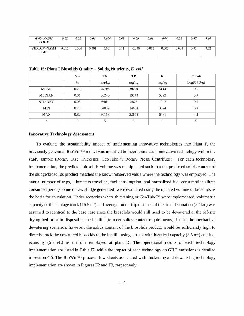
114

AVG÷NASM

LIMIT

0.12 0.02 0.01 0.004 0.69 0.09 0.04 0.04 0.03 0.07 0.10

STD DEV÷NASM

LIMIT 0.015 0.004 0.001 0.001 0.11 0.006 0.005 0.005 0.003 0.01 0.02

Table I6: Plant I Biosolids Quality – Solids, Nutrients, E. coli

VS TN TP K E. coli

% mg/kg mg/kg mg/kg Log(CFU/g)

MEAN 0.79 69186 18794 5114 3.7

MEDIAN 0.81 66240 19274 5323 3.7

STD DEV 0.03 6664 2875 1047 0.2

MIN 0.75 64032 14894 3624 3.4

MAX 0.82 80153 22672 6481 4.1

n 5 5 5 5 5


To evaluate the sustainability impact of implementing innovative technologies into Plant F, the







the basis for calculation. Under scenarios where thickening or GeoTube™ were implemented, volumetric

capacity of the haulage truck (16.5 m3) and average round-trip distance of the final destination (52 km) was

assumed to identical to the base case since the biosolids would still need to be dewatered at the off-site

drying bed prior to disposal at the landfill (to meet solids content requirements). Under the mechanical

dewatering scenarios, however, the solids content of the biosolids product would be sufficiently high to

directly truck the dewatered biosolids to the landfill using a truck with identical capacity (8.5 m3) and fuel

economy (5 km/L) as the one employed at plant D. The operational results of each technology

implementation are listed in Table I7, while the impact of each technology on GHG emissions is detailed

in section 4.6. The BioWin™ process flow sheets associated with thickening and dewatering technology

implementation are shown in Figures F2 and F3, respectively.

115

Table I7: Plant I Innovative Tech Assessment Results

Base

Case

Disc

Thickener

GeoTube™ Fournier

Press

Centrifuge

BioWin TSS % %

4.5 9.2 16.7 22.9

Volume per truck m3 16.5 16.5 16.5 8.5 8.5

Volume per year m3 2039 803 365 201 146

Number of trips to drying bed per year trips /

year

124 49 22 24 17

Kilometers travelled per year km / year 6917 2993 1602 1889 1374



Fuel consumed / dt sludge L / dt 99 43 23 11 7.7

Note: 80 km to landfill for FP and CF options

Figure I2: Plant I Innovative Tech Thickening PFD

Figure I3: Plant I Innovative Tech Dewatering PFD

116

Appendix J

Plant J Summary

Overview

Plant J is an extended aeration WWTP located in Eastern Ontario and operated by OCWA. Normal

sludge handling operations consist of rotary disc thickening, ATAD stabilization, rotary press dewatering,

and on-site storage. During spreading season, the biosolids are hauled and applied to land for agricultural

purposes.

BioWin Modelling



and the corresponding mean observed value (where applicable) is shown in Table J1. The two observed


Figure J1. The predicted values were consistent with observed values.

Table J1: Plant J BioWin Model Results


(2014-2016)

MLSS mg/L 4600 4208, 5374


Dry mass of solids returned per day (rotary

thickener centrate)

kg TSS/d 82 --

Dry mass of solids returned per day (rotary

press centrate)

kg TSS/d 44 --








117

Figure J1: Plant J BioWin Model PFD

Uncertainty

Raw sludge production uncertainty was not calculated directly because limited WAS TSS values were

available. Instead, given that predicted biosolids mass matched the known reported value (393 dt/year) if

average TS values were employed in the reported value calculation, all uncertainty was assumed to be

associated with variation in TS content. To calculate uncertainty, the standard deviation in TS content

(2.3 %) was divided by the mean TS content (17.2%) and converted to a percentage. Using this measure,

the uncertainty was determined to be 13% (sample size, n = 77).

Energy



consumption for each motor of interest (Table J2). The plant does not employ dedicated digester blowers,

therefore, the percentage of air flow to the digester (obtained from plant records) was used to allocate the

fraction of blower electricity consumed by the digester. The total draw for each category of equipment

(stabilization, pumping, aerated holding) was calculated and divided by mass of raw sludge generated daily

(Table J3). Digester electricity consumption was also divided by the daily quantity of VSS destruction to

obtain a measure of energy efficiency (Table J3).

118

Table J2: Plant J Energy Measurements


(V)

Current

(A)

Power

Factor

(PF)

Power

Draw

(kW)

Motor Run-

Time (Hr/d)

Daily Electricity

Consumption

(kWh/d)

Stabilization

Blower (aeration + digester) 589 56.8 0.905 53.6 24 1286

ATAD- Thermaer pump 1 (mixer) 594 22.8 0.908 20.9 24 502

ATAD- Thermaer pump 2 (mixer) 594 22.3 0.908 20.8 24 499

ATAD- SNDR Pump (mixer) 594 14.2 0.908 13.3 24 318

Sub-total (20% of blower

to ATAD)

1576

Pumping

WAS pump 594 4.6 0.7 N/A 5 17

Sub-total 17

Dewatering

Rotary press 594 6.1 0.67 3.9 4 16

Feed Pump 1 594 1.1 0.93 1 4 4

Feed Pump 2 594 1.1 0.93 1 4 4

Conveyor 1 N/A N/A N/A 1.5 4 6

Conveyor 2 N/A N/A N/A 1.5 4 6

Centrate pump 594 3.1 0.601 1.9 4 8

Sub-total 44

Thickening

Rotary drum thickener 594 0.5 0.716 0.55 10 6

Sub-total 6

Odour Control

Biofilter 594 0.5 0.7 0.4 24 9

Sub-total 9

TOTAL 1652

119

Table J3: Plant J Normalized Electricity Consumption


Stabilization 3.76

Pumping 0.04

Dewatering 0.10

Odour Control 0.02

Thickening 0.01

Total 3.93


Chemical Usage

Plant J uses polymer as part of its mechanical thickening and dewatering processes. To determine

normalized consumption for each chemical, process information obtained from the operator was used in

conjunction with raw sludge production. Per conversations with the operator, thickening polymer is dosed

at a rate of 12000 mg polymer per kg of sludge, which corresponds to 12 kg polymer/dt. Per conversations

with the operator, polymer is consumed at a rate of 45 gallons per week, which corresponds to 6.4 gallons

per day (24.3 L/d). Thus, polymer is consumed at a rate of 6.5 kg polymer per day (polymer is 45%

solution). Dividing by the daily mass of raw sludge production (0.42 dt) yields a normalized polymer usage

value of 28 kg polymer/dt. The results are summarized in Table J4.

Table J4: Plant J Chemical Usage

Chemical Value Units

Dewatering Polymer 45 gal /week

6.4 gal/d

24.3 L/d

24.3 kg polymer/d

28 kg polymer/dt raw sludge

Thickening Polymer 12000 mg polymer / kg sludge

0.012 kg polymer / kg sludge

12 kg polymer / dt raw sludge

120



Plant J transports biosolids from the WWTP to agricultural farms during spreading season. During

2014 – 2016, the weighted average round-trip distance between the WWTP and fields was 15.7 km.


Table J5 lists the parameters obtained to calculate normalized transportation fuel consumption. Both









Table J5: Plant J Transportation Fuel Consumption



Volume of biosolids generated per year m3 839.5






Biosolids Quality

A variety of statistical measures detailing the metals content of the hauled biosolids is listed in Table J6.


Table J7.

121

Table J6: Plant J Biosolids Quality – Metals



MEAN 2.2 0.6 1.7 20 425 0.36 2.8 12 28 2.2 326

MEDIAN 2.0 0.5 2.0 19.5 422 0.36 3.0 11 23 2.0 343

STD DEV 0.7 0.1 0.7 4.5 64 0.09 0.9 2.3 18 0.8 71

MIN 0.5 0.5 1.0 9.0 233 0.01 2.0 7.0 1.0 0.60 150

MAX 4 0.9 3.0 32 671 0.70 9.0 19 73 4.0 483

n 81 82 82 82 82 82 82 82 82 81 80

NASM LIMIT 170 34 340 2800 1700 11 94 420 1100 34 4200

AVG÷NASM

LIMIT

0.01 0.02 0.005 0.007 0.25 0.03 0.03 0.03 0.03 0.06 0.08

STD

DEV÷NASM

LIMIT

0.004 0.003 0.002 0.002 0.04 0.01 0.01 0.01 0.02 0.02 0.02

Table J7: Plant J Biosolids Quality – Solids, Nutrients, E. coli

TS TN TP K E. coli


MEAN 17.2 32347 25466 906 2.1

MEDIAN 16.7 30136 25200 900 2.0

STD DEV 2.3 7599 5486 187 0.57

MIN 12.9 19315 10100 0 0.03

MAX 29 60000 47600 1420 3.1

n 77 79 82 82 84

benchmarking the sustainability of sludge handling systems

Documents